ACADEMY OF ACCOUNTING AND FINANCIAL STUDIES JOURNAL

Volume 9, Number 3 ISSN 1096-3685

ACADEMY OF ACCOUNTING ANDFINANCIAL STUDIES JOURNAL

An official Journal of theAllied Academies, Inc.

Michael Grayson, Jackson State UniversityAccounting Editor

Denise Woodbury, Southern Utah UniversityFinance Editor

Academy Informationis published on the Allied Academies web page

www.alliedacademies.org

The Allied Academies, Inc., is a non-profit association of scholars, whose purposeis to support and encourage research and the sharing and exchange of ideas andinsights throughout the world.

Whitney Press, Inc.

Printed by Whitney Press, Inc.PO Box 1064, Cullowhee, NC 28723

www.whitneypress.com

Authors provide the Academy with a publication permission agreement. AlliedAcademies is not responsible for the content of the individual manuscripts. Anyomissions or errors are the sole responsibility of the individual authors. TheEditorial Board is responsible for the selection of manuscripts for publication fromamong those submitted for consideration. The Publishers accept final manuscriptsin digital form and make adjustments solely for the purposes of pagination andorganization.

The Academy of Accounting and Financial Studies Journal is published by theAllied Academies, Inc., PO Box 2689, 145 Travis Road, Cullowhee, NC 28723,(828) 293-9151, FAX (828) 293-9407. Those interested in subscribing to theJournal, advertising in the Journal, submitting manuscripts to the Journal, orotherwise communicating with the Journal, should contact the Executive Directorat [email protected].

Copyright 2005 by the Allied Academies, Inc., Cullowhee, NC

iii

Academy of Accounting and Financial Studies Journal, Volume 9, Number 3, 2005

Academy of Accounting and Financial Studies JournalAccounting Editorial Review Board Members

Agu AnanabaAtlanta Metropolitan CollegeAtlanta, Georgia

Richard FernEastern Kentucky UniversityRichmond, Kentucky

Manoj AnandIndian Institute of ManagementPigdamber, Rau, India

Peter FrischmannIdaho State UniversityPocatello, Idaho

Ali AzadUnited Arab Emirates UniversityUnited Arab Emirates

Farrell GeanPepperdine UniversityMalibu, California

D'Arcy BeckerUniversity of Wisconsin - Eau ClaireEau Claire, Wisconsin

Luis GillmanAerospeedJohannesburg, South Africa

Jan BellCalifornia State University, NorthridgeNorthridge, California

Richard B. GriffinThe University of Tennessee at MartinMartin, Tennessee

Linda BresslerUniversity of Houston-DowntownHouston, Texas

Marek GruszczynskiWarsaw School of EconomicsWarsaw, Poland

Jim BushMiddle Tennessee State UniversityMurfreesboro, Tennessee

Morsheda HassanGrambling State UniversityGrambling, Louisiana

Douglass CagwinLander UniversityGreenwood, South Carolina

Richard T. HenageUtah Valley State CollegeOrem, Utah

Richard A.L. CaldarolaTroy State UniversityAtlanta, Georgia

Rodger HollandGeorgia College & State UniversityMilledgeville, Georgia

Eugene CalvasinaSouthern University and A & M CollegeBaton Rouge, Louisiana

Kathy HsuUniversity of Louisiana at LafayetteLafayette, Louisiana

Darla F. ChisholmSam Houston State UniversityHuntsville, Texas

Shaio Yan HuangFeng Chia UniversityChina

Askar ChoudhuryIllinois State UniversityNormal, Illinois

Robyn HulsartOhio Dominican UniversityColumbus, Ohio

Natalie Tatiana ChurykNorthern Illinois UniversityDeKalb, Illinois

Evelyn C. HumeLongwood UniversityFarmville, Virginia

Prakash DheeriyaCalifornia State University-Dominguez HillsDominguez Hills, California

Terrance JalbertUniversity of Hawaii at HiloHilo, Hawaii

Rafik Z. EliasCalifornia State University, Los AngelesLos Angeles, California

Marianne JamesCalifornia State University, Los AngelesLos Angeles, California

iv

Academy of Accounting and Financial Studies JournalAccounting Editorial Review Board Members


Jongdae JinUniversity of Maryland-Eastern ShorePrincess Anne, Maryland

Ida Robinson-BackmonUniversity of BaltimoreBaltimore, Maryland

Ravi KamathCleveland State UniversityCleveland, Ohio

P.N. SaksenaIndiana University South BendSouth Bend, Indiana

Marla KrautUniversity of IdahoMoscow, Idaho

Martha SaleSam Houston State UniversityHuntsville, Texas

Jayesh KumarXavier Institute of ManagementBhubaneswar, India

Milind SathyeUniversity of CanberraCanberra, Australia

Brian LeeIndiana University KokomoKokomo, Indiana

Junaid M.ShaikhCurtin University of TechnologyMalaysia

Harold LittleWestern Kentucky UniversityBowling Green, Kentucky

Ron StundaBirmingham-Southern CollegeBirmingham, Alabama

C. Angela LetourneauWinthrop UniversityRock Hill, South Carolina

Darshan WadhwaUniversity of Houston-DowntownHouston, Texas

Treba MarshStephen F. Austin State UniversityNacogdoches, Texas

Dan WardUniversity of Louisiana at LafayetteLafayette, Louisiana

Richard MasonUniversity of Nevada, RenoReno, Nevada

Suzanne Pinac WardUniversity of Louisiana at LafayetteLafayette, Louisiana

Richard MautzNorth Carolina A&T State UniversityGreensboro, North Carolina

Michael WattersHenderson State UniversityArkadelphia, Arkansas

Rasheed MblakpoLagos State UniversityLagos, Nigeria

Clark M. WheatleyFlorida International UniversityMiami, Florida

Nancy MeadeSeattle Pacific UniversitySeattle, Washington

Barry H. WilliamsKing’s CollegeWilkes-Barre, Pennsylvania

Thomas PresslyIndiana University of PennsylvaniaIndiana, Pennsylvania

Carl N. WrightVirginia State UniversityPetersburg, Virginia

Hema RaoSUNY-OswegoOswego, New York

v


Academy of Accounting and Financial Studies JournalFinance Editorial Review Board Members

Confidence W. AmadiFlorida A&M UniversityTallahassee, Florida

Ravi KamathCleveland State UniversityCleveland, Ohio

Roger J. BestCentral Missouri State UniversityWarrensburg, Missouri

Jayesh KumarIndira Gandhi Institute of Development ResearchIndia

Donald J. BrownSam Houston State UniversityHuntsville, Texas

William LaingAnderson CollegeAnderson, South Carolina

Richard A.L. CaldarolaTroy State UniversityAtlanta, Georgia

Helen LangeMacquarie UniversityNorth Ryde, Australia

Darla F. ChisholmSam Houston State UniversityHuntsville, Texas

Malek LashgariUniversity of HartfordWest Hartford, Connetticut

Askar ChoudhuryIllinois State UniversityNormal, Illinois

Patricia LobingierGeorge Mason UniversityFairfax, Virginia

Prakash DheeriyaCalifornia State University-Dominguez HillsDominguez Hills, California

Ming-Ming LaiMultimedia UniversityMalaysia

Martine DuchateletBarry UniversityMiami, Florida

Steve MossGeorgia Southern UniversityStatesboro, Georgia

Stephen T. EvansSouthern Utah UniversityCedar City, Utah

Christopher NgassamVirginia State UniversityPetersburg, Virginia

William ForbesUniversity of GlasgowGlasgow, Scotland

Bin PengNanjing University of Science and TechnologyNanjing, P.R.China

Robert GraberUniversity of Arkansas - MonticelloMonticello, Arkansas

Hema RaoSUNY-OswegoOswego, New York

John D. GroesbeckSouthern Utah UniversityCedar City, Utah

Milind SathyeUniversity of CanberraCanberra, Australia

Marek GruszczynskiWarsaw School of EconomicsWarsaw, Poland

Daniel L. TompkinsNiagara UniversityNiagara, New York

Mahmoud HajGrambling State UniversityGrambling, Louisiana

Randall ValentineUniversity of MontevalloPelham, Alabama

Mohammed Ashraful HaqueTexas A&M University-TexarkanaTexarkana, Texas

Marsha WeberMinnesota State University MoorheadMoorhead, Minnesota

Terrance JalbertUniversity of Hawaii at HiloHilo, Hawaii

vi


ACADEMY OF ACCOUNTING ANDFINANCIAL STUDIES JOURNAL

CONTENTS

ACCOUNTING EDITORIAL REVIEW BOARD MEMBERS . . . . . . . . . . . . . . . . . . . . . . . . . iii

FINANCE EDITORIAL REVIEW BOARD MEMBERS . . . . . . . . . . . . . . . . . . . . . . . . . . . . . . v

LETTER FROM THE EDITORS . . . . . . . . . . . . . . . . . . . . . . . . . . . . . . . . . . . . . . . . . . . . . . . viii

THE PERFORMANCE OF AMERICAN DEPOSITORYRECEIPTS LISTED ON THE NEW YORK STOCKEXCHANGE: THE CASE OF UTILITIES . . . . . . . . . . . . . . . . . . . . . . . . . . . . . . . . . . . 1Mark Schaub, Northwestern State UniversityK. Michael Casey, University of Central Arkansas

THE EFFECT OF FINANCIAL INSTITUTIONOBJECTIVES ON EQUITY TURNOVER . . . . . . . . . . . . . . . . . . . . . . . . . . . . . . . . . . . 13Vaughn S. Armstrong, Utah Valley State CollegeNorman Gardner, Utah Valley State College

THE RELATIONSHIP BETWEEN INTEREST RATESON THE NUMBER OF LARGE ANDSMALL BUSINESS FAILURES . . . . . . . . . . . . . . . . . . . . . . . . . . . . . . . . . . . . . . . . . . 29Steven V. Campbell, University of IdahoAskar H. Choudhury, Illinois State University

A MODEL FOR DETERMINATION OF THEQUALITY OF EARNINGS . . . . . . . . . . . . . . . . . . . . . . . . . . . . . . . . . . . . . . . . . . . . . . 41Robert L. Putman, University of Tennessee at MartinRichard B. Griffin, University of Tennessee at MartinRonald W. Kilgore, University of Tennessee at Martin

vii


INVESTOR RISK AVERSION AND THE WEEKENDEFFECT: THE BASICS . . . . . . . . . . . . . . . . . . . . . . . . . . . . . . . . . . . . . . . . . . . . . . . . . 51Michael T. Young, Minnesota State University - Mankato

THE EFFECT OF THE FIRM'S MONOPOLY POWERON THE EARNINGS RESPONSE COEFFICIENT . . . . . . . . . . . . . . . . . . . . . . . . . . . 65Kyung Joo Lee, Cheju National UniversityJongdae Jin, University of Maryland-Eastern ShoreSung K. Huh, California State University-San Bernardino

BRAND VALUE AND THE REPRESENTATIONALFAITHFULNESS OF BALANCE SHEETS . . . . . . . . . . . . . . . . . . . . . . . . . . . . . . . . . . 79Philip Little, Western Carolina UniversityDavid Coffee, Western Carolina UniversityRoger Lirely, Western Carolina University

WHAT PUTS THE CONVENIENCE INCONVENIENCE YIELDS? . . . . . . . . . . . . . . . . . . . . . . . . . . . . . . . . . . . . . . . . . . . . . . 89Bahram Adrangi, University of PortlandArjun Chatrath, University of PortlandRohan Christie-David, Louisiana Tech UniversityWilliam T. Moore, University of South Carolina

THE IMPACT OF CURRENT TAX POLICY ON CEOSTOCK OPTION COMPENSATION:A QUANTILE ANALYSIS . . . . . . . . . . . . . . . . . . . . . . . . . . . . . . . . . . . . . . . . . . . . . . 119Martin Gritsch, William Patterson UniversityTricia Coxwell Snyder, William Paterson University

viii


LETTER FROM THE EDITORS

Welcome to the Academy of Accounting and Financial Studies Journal, an official journalof the Allied Academies, Inc., a non profit association of scholars whose purpose is to encourageand support the advancement and exchange of knowledge, understanding and teaching throughoutthe world. The AAFSJ is a principal vehicle for achieving the objectives of the organization. Theeditorial mission of this journal is to publish empirical and theoretical manuscripts which advancethe disciplines of accounting and finance.

Dr. Michael Grayson, Jackson State University, is the Accountancy Editor and Dr. DeniseWoodbury, Southern Utah University, is the Finance Editor. Their joint mission is to make theAAFSJ better known and more widely read.

As has been the case with the previous issues of the AAFSJ, the articles contained in thisvolume have been double blind refereed. The acceptance rate for manuscripts in this issue, 25%,conforms to our editorial policies.

The Editors work to foster a supportive, mentoring effort on the part of the referees whichwill result in encouraging and supporting writers. They will continue to welcome differentviewpoints because in differences we find learning; in differences we develop understanding; indifferences we gain knowledge and in differences we develop the discipline into a morecomprehensive, less esoteric, and dynamic metier.

Information about the Allied Academies, the AAFSJ, and the other journals published by theAcademy, as well as calls for conferences, are published on our web site. In addition, we keep theweb site updated with the latest activities of the organization. Please visit our site and know that wewelcome hearing from you at any time.

Michael Grayson, Jackson State University

Denise Woodbury, Southern Utah University


1


THE PERFORMANCE OF AMERICAN DEPOSITORYRECEIPTS LISTED ON THE NEW YORK STOCK

EXCHANGE: THE CASE OF UTILITIES

Mark Schaub, Northwestern State UniversityK. Michael Casey, University of Central Arkansas

ABSTRACT

In this study, we test the early and aftermarket returns of utility company AmericanDepository Receipts (ADRs) issued from January 1987 through September 2000 and traded on theNew York Stock Exchange. The results are broken down to compare IPOs versus SEOs andemerging market firms versus developed market firms. Findings indicate that utility industry ADRssignificantly underperform the S&P 500 in the early trading, with the entire sample returning 5.35percentage points less than the market index in the first month of trading. IPOs perform worse thanSEOs and developed market issues perform worse than emerging market utility industry ADRs inthe short-run.

Over the three-year holding period from date of issue, developed market utility ADRs tendto underperform those issued in emerging markets and utility SEOs underperform IPOs. The entireutility ADR sample underperformed the S&P 500 index by 23 percentage points in the three-yeartrading horizon. Essentially, our study shows foreign utility-firm ADRs initially listed on the NYSEfrom 1987 through mid-2000 underperformed the S&P 500 at the time of listing and for thethree-year period following.

INTRODUCTION

The utilities industry consists of mostly large firms with strong, non-volatile earnings. Oftenregulated and in many cases with monopoly power (at least locally), utilities firms are unique in theUnited States, providing a safe stream of income to investors. But how do foreign utilities firmscompare? The purpose of this study is to answer this question by reporting and statistically testingthe early and long-term performance of foreign utility industry equities traded in the US as AmericanDepository Receipts relative to the performance of the S&P 500 market index.

We examine daily returns for the first month, and monthly returns for three years after theissue date of non-US utility equities listed on the New York Stock Exchange (NYSE). These returnsare adjusted based on the corresponding returns of the S&P 500 index to determine the excess returnof foreign utility stocks relative to the market return. The excess return results are segmented to

2


compare foreign utility IPO issues to those that are seasoned equity offerings (SEOs) and equitiesthat were issued by firms headquartered in emerging countries to those from developed countries.

LITERATURE REVIEW

ADR Studies

American Depository Receipts (ADRs) represent ownership of foreign equities held ondeposit by large custodian banks in the United States. Each receipt is backed by various sharequantities of foreign stock bundled to reflect average common share prices in US equity markets.The primary purpose of ADR creation is to enable U.S. investors to participate in foreign equitieswithout dealing directly with the foreign exchange and currency markets.

Several ADR studies examine ADR returns relative to a market benchmark using standardIPO methodology. Callaghan, Kleiman and Sahu (1999) reported positive market-adjusted returnsfor ADRs in the early and long-term investment horizons and found emerging market ADR returnsto be higher than those for firms from developed countries. Specifically, they report one-dayabnormal returns of 5.29% and one-month cumulative daily returns of 2.35% for a sample of 66ADRs issued from 18 different countries and traded on the NYSE, the AMEX and the NASDAQfrom 1986 to 1993. Annually, they found the cumulative abnormal returns for NYSE-traded ADRswere 19.6% for the first year; with the 12-month cumulative abnormal return for ADRs issued byfirms in countries considered emerging markets at 34.37%.

Foerster and Karolyi (2000) found ADRs underperform comparable firms by 8% to 15%during the three-year period following the date of issuance, in contrast to the Callaghan et al. (1999)study. They examined ADR returns for a full three years from the issue date for a sample of 333global equity offerings listed from 1982 through 1996 and including ADRs from 35 countries inAsia, Latin America and Europe. Their entire sample accumulated 1-month excess returns of-1.13% and 12-month cumulative abnormal returns of -4.07% relative to the index benchmark. The36-month underperformance was significant with cumulative abnormal returns of -14.99% basedon a local index. When compared to a US index, the cumulative abnormal returns for the ADRswere -27.53% for the three-year holding period.

Schaub and Casey (2002), Schaub (2003), and Schaub, Casey and Heslop (2004) performedindustry specific ADR studies. Schaub and Casey (2002) examined short-term returns for foreignoil and gas firms listed on the New York Stock Exchange and found there was no significantdifference in the performance of those firms and the S&P 500 index for the first 25 days of trading.Schaub (2003) found similar short-term results for 32 foreign bank equities listed on the New YorkStock Exchange. In the long term, Schaub et al. (2004) found 34 foreign oil and gas equitiesperformed roughly the same as the S&P 500 index for the first three years of trading from the dateof listing on the New York Stock Exchange.

3


IPO Studies

Because ADR research uses similar methodologies as IPO studies, the results of research inthe area of IPOs may be comparable to those of this study. Most research has found significantshort-term abnormal positive returns for initial public offerings (IPOs), including Neuberger and LaChapelle (1983), McDonald and Fisher (1972), Neuberger and Hammond (1974), Reilly (1977),Logue (1973), Ibbotson (1975), Ibbotson and Jaffe (1975), Ritter (1984), Miller and Reilly (1987),and Ibbotson, Sindelar and Ritter (1988) examine IPO early returns. Short term results suggestfirst-day IPO abnormal returns in US markets range from as low as .60% (Barry and Jennings 1993)to 26.5% (Ritter 1984) and five-day cumulative abnormal returns range from 5.09% (Block andStanley 1980) to 28.5% (McDonald and Fisher 1972).

In the long-run IPO studies, Ritter (1991) examined the long-term performance of IPOs andfound that, from the first day of trading to the third anniversary, a sample of 1,526 IPOs issued from1975-84 underperformed the benchmark by 27.4%. Essentially, Ritter's (1991) findings suggest theearly positive abnormal performance of IPOs does not hold over the long term, and has foundagreement from Brav and Gompers (1997).

Studies of foreign IPO behavior produced similar conclusions. Aggarwal, Leal andHernandez (1993) found 62 Brazilian IPOs, 36 Chilean IPOs, and 44 Mexican IPOs significantlyoutperformed the local benchmark the first day of trading, but significantly underperformed the samebenchmark after three years of trading. Other studies provide additional evidence of long-rununderperformance of IPOs in foreign equity markets, including Levis (1993) and Huang (1999) whoexamined the UK amd Taiwan IPO performance respecitively. Studies that report differing resultsfor the long-term IPO performance include Ben Naceur (2000), who examined the Tunisian market,and Dawson (1987), who reported long-term positive abnormal returns for IPOs traded in Malaysia.

RESEARCH METHODOLOGY

This study investigates the early and long-run abnormal returns of foreign utility industrynew equity issues traded on the New York Stock Exchange. The sample consists of 24 ADRsinitially listed on the New York Stock Exchange from January 1, 1987 through September 30, 2000.Of the 24 ADRs, 15 are initial public offerings (IPOs) and 9 are seasoned equity offerings (SEOs). The emerging markets sample size contains 8 firms and the developed market ADRs make up theremaining 16. Table 1 gives a further breakdown of the sample composition.

Standard IPO event study methodology was followed to compute and test the abnormalreturns of the foreign equity portfolios. The daily and monthly holding period returns for eachsecurity are computed first. Then, daily abnormal returns are computed by subtracting the dailyreturns of each security from that of the S&P 500. The monthly abnormal returns are computed by

4


subtracting each monthly holding period return from that of the S&P 500 index. The S&P 500proxies the market return because the ADR sample includes only firms listed on the NYSE.

Table 1Sample Description by Type of Issue and Level of Issue

Column 1 Column 2 Column 3 Column 4

ADR Type of Issue Emerging Sample Developed Sample Total ADRs

IPO 7 8 15

SEO 1 8 9

Totals 8 16 24

Equations 1 through 3 describe the process for computing abnormal returns and cumulativeabnormal returns for statistical testing. The abnormal return for each security i on day t (arit) iscomputed as the return of the security on day t (rit ) minus the return of the market on day t (rmt) asshown in equation 1 below. For computing monthly abnormal returns, t represents the respectivemonth.

(1)rrar mtitit−=

Equation 2 computes the average abnormal return for the sample for day/month t (ARt) asthe equally-weighted arithmetic average of the abnormal returns of each of the n securities duringday/month t.

(2)∑=

=n

iitt arAR n 1

1

Cumulative abnormal returns as of day/month s are computed as the summation of theaverage abnormal returns starting at day/month 1 until day/month s in Equation 3.

(3)∑=

=s

ts ARCAR t

1,1

Daily/monthly average abnormal returns and the cumulative abnormal returns are tested todetermine significance using a Z-score. The respective p-values for these tests are reported. A p-value of .10 or less indicates the abnormal return or cumulative abnormal return is significantlydifferent from 0.

5


THE ANALYSIS

Results From Early Trading

Tables 2 through 5 summarize the early and aftermarket performance of the equities by typeof issue and type of market. Contrary to the results of other ADR studies and most IPO research,the abnormal return on the first day of trading was small and non-significant for the entire sample,as reported in Table 2. This finding suggests the average NYSE-traded foreign utility equity issuereturned roughly the same as the S&P 500.

Table 2. The Early Return Performance By Day For the Entire Sample, IPO and SEO Utilities IssuesEntire ADR Sample (Obs = 24) ADRs Issued as IPOs (Obs = 15) ADRs Issued as SEOs (Obs = 9)

Day AR P-value CAR P-value AR P-value CAR P-value AR P-value CAR P-value

D1 -0.82% 0.16 -0.82% 0.16 -1.32% 0.17 -1.32% 0.17 -0.15% 0.39 -0.15% 0.39

D2 -1.21% 0.02 -2.03% 0.02 -0.70% 0.22 -2.02% 0.11 -2.11% 0.00 -2.26% 0.00D3 -0.27% 0.24 -2.30% 0.02 -0.10% 0.44 -2.12% 0.11 -0.70% 0.14 -2.96% 0.00D4 -1.47% 0.01 -3.77% 0.00 -1.74% 0.01 -3.86% 0.02 -0.93% 0.21 -3.89% 0.00D5 0.16% 0.48 -3.61% 0.00 0.20% 0.40 -3.66% 0.04 -0.25% 0.25 -4.15% 0.00D6 -0.82% 0.02 -4.43% 0.00 -1.07% 0.04 -4.73% 0.01 -0.47% 0.12 -4.62% 0.00D7 -0.17% 0.35 -4.60% 0.00 0.12% 0.42 -4.60% 0.02 -0.70% 0.18 -5.32% 0.00D8 -0.55% 0.17 -5.16% 0.00 -0.03% 0.48 -4.63% 0.02 -1.45% 0.05 -6.77% 0.00D9 0.33% 0.23 -4.83% 0.00 0.44% 0.25 -4.20% 0.04 0.19% 0.39 -6.58% 0.00

D10 -0.02% 0.52 -4.85% 0.00 -0.12% 0.40 -4.32% 0.04 0.27% 0.35 -6.32% 0.00D11 0.62% 0.11 -4.22% 0.01 0.45% 0.29 -3.87% 0.07 1.03% 0.03 -5.29% 0.01D12 -0.36% 0.09 -4.58% 0.01 -0.22% 0.29 -4.09% 0.06 -0.70% 0.04 -5.98% 0.01D13 -0.11% 0.38 -4.69% 0.01 0.05% 0.46 -4.04% 0.07 -0.36% 0.22 -6.34% 0.00D14 0.37% 0.18 -4.32% 0.01 -0.16% 0.39 -4.20% 0.06 1.53% 0.04 -4.82% 0.03D15 -0.35% 0.14 -4.67% 0.01 -0.44% 0.14 -4.64% 0.05 -0.41% 0.31 -5.22% 0.03D16 -0.23% 0.26 -4.90% 0.01 -0.40% 0.19 -5.05% 0.04 0.02% 0.49 -5.20% 0.03D17 0.14% 0.45 -4.77% 0.01 -0.45% 0.30 -5.49% 0.03 0.93% 0.01 -4.27% 0.07D18 -0.17% 0.36 -4.94% 0.01 -0.07% 0.46 -5.56% 0.03 -0.35% 0.28 -4.62% 0.06D19 0.10% 0.41 -4.84% 0.01 0.37% 0.25 -5.19% 0.05 -0.35% 0.34 -4.98% 0.05D20 -0.46% 0.17 -5.30% 0.01 -0.36% 0.23 -5.55% 0.04 -0.64% 0.27 -5.62% 0.04D21 -0.05% 0.41 -5.35% 0.01 -0.48% 0.13 -6.03% 0.03 0.58% 0.19 -5.04% 0.06The computation of average abnormal returns (AR) is described in equation 2 in the text and the computation of cumulativeabnormal returns (CAR) is described in equation 3 in the text. P-values in bold italics represent returns that are significant at analpha level of 10% or lower.

6


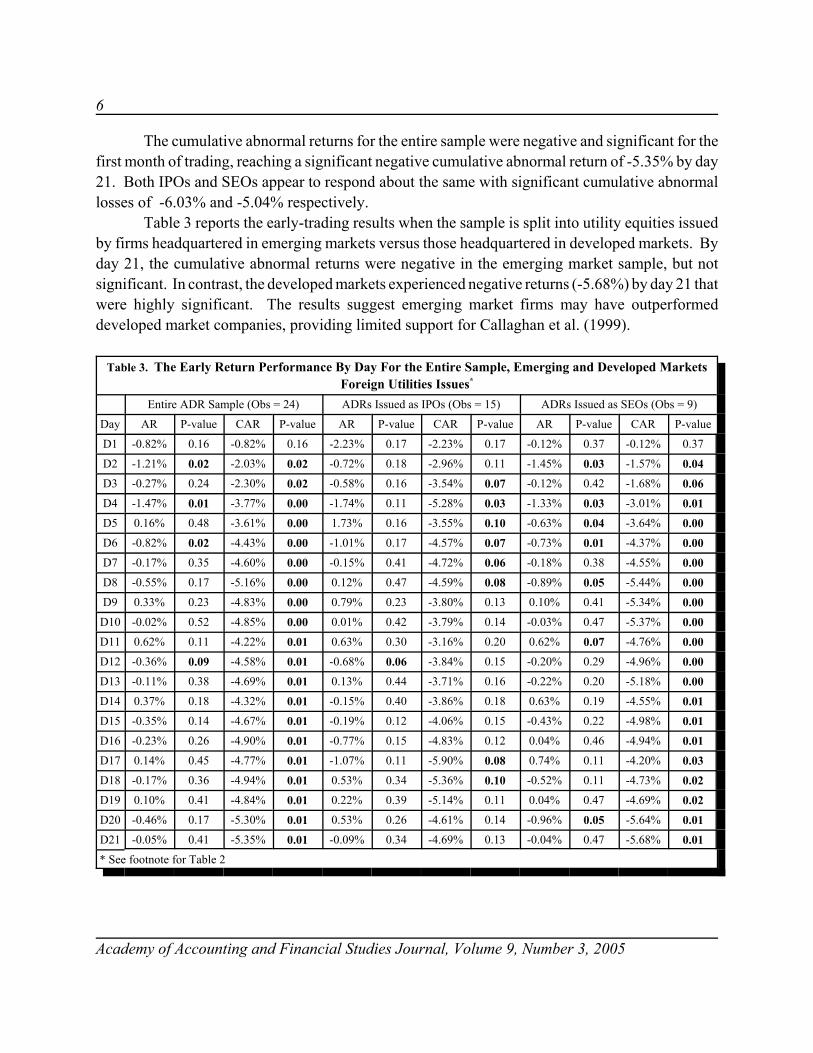
The cumulative abnormal returns for the entire sample were negative and significant for thefirst month of trading, reaching a significant negative cumulative abnormal return of -5.35% by day21. Both IPOs and SEOs appear to respond about the same with significant cumulative abnormallosses of -6.03% and -5.04% respectively.

Table 3 reports the early-trading results when the sample is split into utility equities issuedby firms headquartered in emerging markets versus those headquartered in developed markets. Byday 21, the cumulative abnormal returns were negative in the emerging market sample, but notsignificant. In contrast, the developed markets experienced negative returns (-5.68%) by day 21 thatwere highly significant. The results suggest emerging market firms may have outperformeddeveloped market companies, providing limited support for Callaghan et al. (1999).

Table 3. The Early Return Performance By Day For the Entire Sample, Emerging and Developed MarketsForeign Utilities Issues*

Entire ADR Sample (Obs = 24) ADRs Issued as IPOs (Obs = 15) ADRs Issued as SEOs (Obs = 9)

Day AR P-value CAR P-value AR P-value CAR P-value AR P-value CAR P-value

D1 -0.82% 0.16 -0.82% 0.16 -2.23% 0.17 -2.23% 0.17 -0.12% 0.37 -0.12% 0.37

D2 -1.21% 0.02 -2.03% 0.02 -0.72% 0.18 -2.96% 0.11 -1.45% 0.03 -1.57% 0.04D3 -0.27% 0.24 -2.30% 0.02 -0.58% 0.16 -3.54% 0.07 -0.12% 0.42 -1.68% 0.06D4 -1.47% 0.01 -3.77% 0.00 -1.74% 0.11 -5.28% 0.03 -1.33% 0.03 -3.01% 0.01D5 0.16% 0.48 -3.61% 0.00 1.73% 0.16 -3.55% 0.10 -0.63% 0.04 -3.64% 0.00D6 -0.82% 0.02 -4.43% 0.00 -1.01% 0.17 -4.57% 0.07 -0.73% 0.01 -4.37% 0.00D7 -0.17% 0.35 -4.60% 0.00 -0.15% 0.41 -4.72% 0.06 -0.18% 0.38 -4.55% 0.00D8 -0.55% 0.17 -5.16% 0.00 0.12% 0.47 -4.59% 0.08 -0.89% 0.05 -5.44% 0.00D9 0.33% 0.23 -4.83% 0.00 0.79% 0.23 -3.80% 0.13 0.10% 0.41 -5.34% 0.00

D10 -0.02% 0.52 -4.85% 0.00 0.01% 0.42 -3.79% 0.14 -0.03% 0.47 -5.37% 0.00D11 0.62% 0.11 -4.22% 0.01 0.63% 0.30 -3.16% 0.20 0.62% 0.07 -4.76% 0.00D12 -0.36% 0.09 -4.58% 0.01 -0.68% 0.06 -3.84% 0.15 -0.20% 0.29 -4.96% 0.00D13 -0.11% 0.38 -4.69% 0.01 0.13% 0.44 -3.71% 0.16 -0.22% 0.20 -5.18% 0.00D14 0.37% 0.18 -4.32% 0.01 -0.15% 0.40 -3.86% 0.18 0.63% 0.19 -4.55% 0.01D15 -0.35% 0.14 -4.67% 0.01 -0.19% 0.12 -4.06% 0.15 -0.43% 0.22 -4.98% 0.01D16 -0.23% 0.26 -4.90% 0.01 -0.77% 0.15 -4.83% 0.12 0.04% 0.46 -4.94% 0.01D17 0.14% 0.45 -4.77% 0.01 -1.07% 0.11 -5.90% 0.08 0.74% 0.11 -4.20% 0.03D18 -0.17% 0.36 -4.94% 0.01 0.53% 0.34 -5.36% 0.10 -0.52% 0.11 -4.73% 0.02D19 0.10% 0.41 -4.84% 0.01 0.22% 0.39 -5.14% 0.11 0.04% 0.47 -4.69% 0.02D20 -0.46% 0.17 -5.30% 0.01 0.53% 0.26 -4.61% 0.14 -0.96% 0.05 -5.64% 0.01D21 -0.05% 0.41 -5.35% 0.01 -0.09% 0.34 -4.69% 0.13 -0.04% 0.47 -5.68% 0.01* See footnote for Table 2

7


Results From Aftermarket Trading

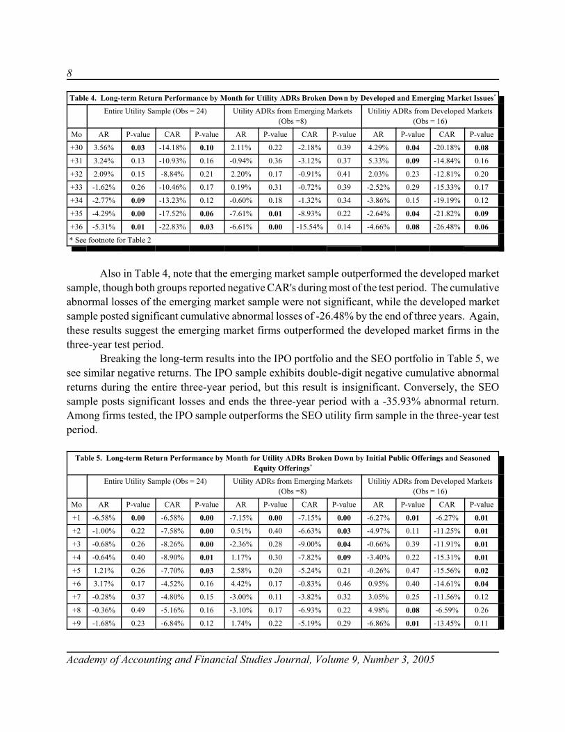
Tables 4 and 5 show the long-term results of the foreign utility issues by month for the first3 years of trading on the New York Stock Exchange. The results, reported for the entire sample inTable 4, suggest the securities substantially underperformed the S&P 500 during this period. Thecumulative abnormal returns by the end of the three-year period were -22.83% and statisticallysignificant.

Table 4. Long-term Return Performance by Month for Utility ADRs Broken Down by Developed and Emerging Market Issues*

Entire Utility Sample (Obs = 24) Utility ADRs from Emerging Markets(Obs =8)

Utilitiy ADRs from Developed Markets(Obs = 16)

Mo AR P-value CAR P-value AR P-value CAR P-value AR P-value CAR P-value

+1 -6.58% 0.00 -6.58% 0.00 -6.82% 0.02 -6.82% 0.02 -6.45% 0.00 -6.45% 0.00

+2 -1.00% 0.22 -7.58% 0.00 0.68% 0.41 -6.15% 0.07 -1.84% 0.21 -8.30% 0.00

+3 -0.68% 0.26 -8.26% 0.00 -4.37% 0.15 -10.52% 0.04 1.16% 0.23 -7.13% 0.02

+4 -0.64% 0.40 -8.90% 0.01 -0.62% 0.47 -11.14% 0.05 -0.65% 0.40 -7.79% 0.04

+5 1.21% 0.26 -7.70% 0.03 2.31% 0.24 -8.83% 0.12 0.65% 0.40 -7.13% 0.09

+6 3.17% 0.17 -4.52% 0.16 0.28% 0.49 -8.55% 0.13 4.62% 0.15 -2.51% 0.36

+7 -0.28% 0.37 -4.80% 0.15 -3.69% 0.10 -12.24% 0.07 1.43% 0.30 -1.08% 0.44

+8 -0.36% 0.49 -5.16% 0.16 -3.54% 0.33 -15.78% 0.06 1.23% 0.31 0.15% 0.49

+9 -1.68% 0.23 -6.84% 0.12 3.15% 0.10 -12.62% 0.11 -4.10% 0.04 -3.95% 0.32

+10 7.88% 0.05 1.04% 0.46 19.78% 0.05 7.15% 0.47 1.93% 0.24 -2.02% 0.41

+11 0.15% 0.50 1.18% 0.46 -1.05% 0.24 6.10% 0.50 0.75% 0.31 -1.27% 0.44

+12 1.39% 0.32 2.57% 0.49 2.17% 0.33 8.27% 0.47 1.00% 0.39 -0.27% 0.49

+13 -1.16% 0.29 1.42% 0.48 -3.91% 0.21 4.36% 0.47 0.22% 0.43 -0.05% 0.50

+14 -2.66% 0.08 -1.24% 0.38 -3.02% 0.30 1.34% 0.43 -2.48% 0.08 -2.53% 0.40

+15 2.63% 0.12 1.39% 0.49 0.93% 0.44 2.26% 0.45 3.48% 0.10 0.95% 0.46

+16 -0.47% 0.35 0.92% 0.45 -4.54% 0.03 -2.27% 0.34 1.56% 0.29 2.52% 0.40

+17 -0.80% 0.44 0.11% 0.44 4.01% 0.01 1.73% 0.44 -3.21% 0.08 -0.69% 0.47

+18 -1.92% 0.22 -1.81% 0.38 1.64% 0.30 3.37% 0.49 -3.70% 0.04 -4.40% 0.34

+19 -3.53% 0.02 -5.34% 0.25 -0.83% 0.30 2.54% 0.46 -4.88% 0.01 -9.28% 0.20

+20 -1.67% 0.20 -7.01% 0.20 -5.79% 0.01 -3.25% 0.35 0.39% 0.45 -8.89% 0.22

+21 0.68% 0.40 -6.33% 0.23 2.06% 0.20 -1.19% 0.38 0.00% 0.50 -8.90% 0.23

+22 -3.37% 0.06 -9.70% 0.15 -4.10% 0.02 -5.29% 0.31 -3.00% 0.16 -11.90% 0.17

+23 0.29% 0.49 -9.41% 0.15 -0.41% 0.33 -5.70% 0.30 0.64% 0.40 -11.26% 0.19

+24 -3.82% 0.01 -13.23% 0.09 -5.16% 0.05 -10.86% 0.22 -3.15% 0.06 -14.41% 0.13

+25 -1.91% 0.11 -15.14% 0.06 0.88% 0.47 -9.98% 0.22 -3.31% 0.05 -17.72% 0.09

+26 2.01% 0.13 -13.13% 0.10 8.27% 0.00 -1.71% 0.37 -1.11% 0.32 -18.83% 0.08

+27 0.09% 0.40 -13.04% 0.11 1.27% 0.20 -0.44% 0.41 -0.50% 0.43 -19.34% 0.08

+28 -2.15% 0.11 -15.19% 0.08 -4.40% 0.07 -4.84% 0.33 -1.02% 0.33 -20.36% 0.07

+29 -2.55% 0.08 -17.74% 0.05 0.55% 0.33 -4.28% 0.34 -4.11% 0.06 -24.47% 0.04

8

Table 4. Long-term Return Performance by Month for Utility ADRs Broken Down by Developed and Emerging Market Issues*





+30 3.56% 0.03 -14.18% 0.10 2.11% 0.22 -2.18% 0.39 4.29% 0.04 -20.18% 0.08

+31 3.24% 0.13 -10.93% 0.16 -0.94% 0.36 -3.12% 0.37 5.33% 0.09 -14.84% 0.16

+32 2.09% 0.15 -8.84% 0.21 2.20% 0.17 -0.91% 0.41 2.03% 0.23 -12.81% 0.20

+33 -1.62% 0.26 -10.46% 0.17 0.19% 0.31 -0.72% 0.39 -2.52% 0.29 -15.33% 0.17

+34 -2.77% 0.09 -13.23% 0.12 -0.60% 0.18 -1.32% 0.34 -3.86% 0.15 -19.19% 0.12

+35 -4.29% 0.00 -17.52% 0.06 -7.61% 0.01 -8.93% 0.22 -2.64% 0.04 -21.82% 0.09

+36 -5.31% 0.01 -22.83% 0.03 -6.61% 0.00 -15.54% 0.14 -4.66% 0.08 -26.48% 0.06

* See footnote for Table 2

Also in Table 4, note that the emerging market sample outperformed the developed marketsample, though both groups reported negative CAR's during most of the test period. The cumulativeabnormal losses of the emerging market sample were not significant, while the developed marketsample posted significant cumulative abnormal losses of -26.48% by the end of three years. Again,these results suggest the emerging market firms outperformed the developed market firms in thethree-year test period.

Breaking the long-term results into the IPO portfolio and the SEO portfolio in Table 5, wesee similar negative returns. The IPO sample exhibits double-digit negative cumulative abnormalreturns during the entire three-year period, but this result is insignificant. Conversely, the SEOsample posts significant losses and ends the three-year period with a -35.93% abnormal return.Among firms tested, the IPO sample outperforms the SEO utility firm sample in the three-year testperiod.

Table 5. Long-term Return Performance by Month for Utility ADRs Broken Down by Initial Public Offerings and SeasonedEquity Offerings*




+1 -6.58% 0.00 -6.58% 0.00 -7.15% 0.00 -7.15% 0.00 -6.27% 0.01 -6.27% 0.01

+2 -1.00% 0.22 -7.58% 0.00 0.51% 0.40 -6.63% 0.03 -4.97% 0.11 -11.25% 0.01

+3 -0.68% 0.26 -8.26% 0.00 -2.36% 0.28 -9.00% 0.04 -0.66% 0.39 -11.91% 0.01

+4 -0.64% 0.40 -8.90% 0.01 1.17% 0.30 -7.82% 0.09 -3.40% 0.22 -15.31% 0.01

+5 1.21% 0.26 -7.70% 0.03 2.58% 0.20 -5.24% 0.21 -0.26% 0.47 -15.56% 0.02

+6 3.17% 0.17 -4.52% 0.16 4.42% 0.17 -0.83% 0.46 0.95% 0.40 -14.61% 0.04

+7 -0.28% 0.37 -4.80% 0.15 -3.00% 0.11 -3.82% 0.32 3.05% 0.25 -11.56% 0.12

+8 -0.36% 0.49 -5.16% 0.16 -3.10% 0.17 -6.93% 0.22 4.98% 0.08 -6.59% 0.26

+9 -1.68% 0.23 -6.84% 0.12 1.74% 0.22 -5.19% 0.29 -6.86% 0.01 -13.45% 0.11

9

Table 5. Long-term Return Performance by Month for Utility ADRs Broken Down by Initial Public Offerings and SeasonedEquity Offerings*





+10 7.88% 0.05 1.04% 0.46 6.03% 0.12 0.84% 0.47 9.66% 0.12 -3.79% 0.39

+11 0.15% 0.50 1.18% 0.46 -0.15% 0.46 0.69% 0.47 0.23% 0.46 -3.56% 0.40

+12 1.39% 0.32 2.57% 0.49 -1.11% 0.35 -0.41% 0.49 5.10% 0.16 1.54% 0.46

+13 -1.16% 0.29 1.42% 0.48 -1.33% 0.27 -1.74% 0.44 0.03% 0.49 1.57% 0.46

+14 -2.66% 0.08 -1.24% 0.38 -2.59% 0.11 -4.33% 0.35 -1.75% 0.26 -0.19% 0.50

+15 2.63% 0.12 1.39% 0.49 1.52% 0.28 -2.81% 0.41 4.15% 0.13 3.96% 0.40

+16 -0.47% 0.35 0.92% 0.45 0.01% 0.50 -2.80% 0.41 -2.31% 0.22 1.65% 0.46

+17 -0.80% 0.44 0.11% 0.44 2.53% 0.12 -0.27% 0.49 -5.04% 0.05 -3.39% 0.42

+18 -1.92% 0.22 -1.81% 0.38 -1.81% 0.28 -2.08% 0.44 -1.42% 0.28 -4.81% 0.39

+19 -3.53% 0.02 -5.34% 0.25 -1.55% 0.24 -3.63% 0.39 -7.50% 0.00 -12.31% 0.23

+20 -1.67% 0.20 -7.01% 0.20 -4.40% 0.08 -8.03% 0.27 2.34% 0.16 -9.96% 0.28

+21 0.68% 0.40 -6.33% 0.23 -1.57% 0.29 -9.60% 0.24 4.25% 0.19 -5.71% 0.37

+22 -3.37% 0.06 -9.70% 0.15 -4.12% 0.01 -13.72% 0.16 -1.97% 0.35 -7.68% 0.34

+23 0.29% 0.49 -9.41% 0.15 2.39% 0.17 -11.32% 0.21 -3.89% 0.06 -11.57% 0.27

+24 -3.82% 0.01 -13.23% 0.09 -4.13% 0.02 -15.46% 0.14 -3.27% 0.13 -14.84% 0.21

+25 -1.91% 0.11 -15.14% 0.06 -1.01% 0.35 -16.47% 0.13 -4.47% 0.03 -19.31% 0.15

+26 2.01% 0.13 -13.13% 0.10 3.77% 0.09 -12.70% 0.19 0.18% 0.48 -19.14% 0.16

+27 0.09% 0.40 -13.04% 0.11 0.79% 0.38 -11.91% 0.21 0.15% 0.49 -18.99% 0.17

+28 -2.15% 0.11 -15.19% 0.08 -3.82% 0.05 -15.73% 0.15 -0.03% 0.50 -19.02% 0.17

+29 -2.55% 0.08 -17.74% 0.05 -1.88% 0.21 -17.61% 0.12 -3.61% 0.12 -22.63% 0.13

+30 3.56% 0.03 -14.18% 0.10 3.90% 0.05 -13.72% 0.19 3.49% 0.16 -19.14% 0.17

+31 3.24% 0.13 -10.93% 0.16 5.49% 0.10 -8.22% 0.30 -0.58% 0.42 -19.72% 0.17

+32 2.09% 0.15 -8.84% 0.21 1.59% 0.21 -6.64% 0.34 2.92% 0.25 -16.81% 0.21

+33 -1.62% 0.26 -10.46% 0.17 -0.51% 0.40 -7.14% 0.33 -4.66% 0.28 -21.46% 0.17

+34 -2.77% 0.09 -13.23% 0.12 -2.99% 0.07 -10.14% 0.27 -4.78% 0.24 -26.24% 0.13

+35 -4.29% 0.00 -17.52% 0.06 -4.62% 0.02 -14.75% 0.19 -4.66% 0.01 -30.90% 0.09

+36 -5.31% 0.01 -22.83% 0.03 -6.23% 0.01 -20.98% 0.11 -5.03% 0.16 -35.93% 0.07

* See footnote for Table 2

SUMMARY

Previous ADR and IPO studies reported significant abnormal returns in the early trading.Likewise, most aftermarket IPO studies reported long-run underperformance for IPO portfolios ascompared to market benchmarks. Callaghan, Kleiman and Sahu (1999) reported one-day andone-year positive abnormal returns for a sample of 66 ADRs issued from 18 different countries and

10


traded on the NYSE, the AMEX and the NASDAQ from 1986 to 1993. They found that theemerging market ADRs outperformed the ADRs backed by securities traded in mature markets.This study, confining its sample to utility companies, finds a similar pattern of results in both earlytrading and at three years after listing of the ADR.

The results of this study provide some evidence that the US markets overprice non-US utilityequities across the entire time horizon of this study and provides substantial support for Foerster andKarolyi (2000). Although the sample included all utility ADRs issued on the NYSE from January1987 through September 2000, these results should be interpreted with caution since the sample size,particularly when broken down, is small. Perhaps a larger sample might shed additional light onwhy utility ADRs appear to be overpriced at issue and go on to substantially underperform themarket.

REFERENCES

Aggarwal, R., R. Leal and L. Hernandez (1993). The aftermarket performance of initial public offerings in LatinAmerica. Financial Management, 22, 42-53.

Barry, C. and R. Jennings (1993). The opening price performance of initial public offerings of common stock. FinancialManagement, 22, 54-63.

Ben Naceur, S (2000). An examination of the Tunisian IPO pricing in the short and long run: 1992-1997. AppliedEconomics Letters, 7, 293-296.

Bhandari, A., T. Grammatikos, A. Makhija and G. Papaloannou (1989). Risk and return on newly listed stocks: the post-listing experience. Journal of Financial Research, 12, 93-102.

Block, S. and M. Stanley (1980). The financial characteristics and price movement patterns of companies approachingthe unseasoned securities market in the late 1970's. Financial Management, 30-36.

Brav, A. and P. Gompers (1997). Myth or reality? The long-run underperformance of initial public offerings: evidencefrom venture and nonventure capital-backed companies. Journal of Finance, 52, 1791-1821.

Callaghan, J., R. Kleiman, and A. Sahu (1999). The market-adjusted investment performance of ADR IPOs and SEOs,Global Finance Journal, 10 (2), 123-145.

Dawson, S (1987). The secondary stock market performance of initial public offerings in Hong Kong, Singapore andMalaysia: 1978-1984. Journal of Business, Finance & Accounting, 65-76.

Foerster, S. and A. Karolyi (2000). The long-run performance of global equity offerings. Journal of Financial andQuantitative Analysis, 35, 499-528.

Huang, Y. (1999). The price behavior of initial public offerings on the Taiwan Stock Exchange. Applied FinancialEconomics, 9, 201-208.

11


Ibbotson, R. (1975). Price performance of common stock new issues. Journal of Financial Economics, 235-272.

Ibbotson, R. and J. Jaffe (1975). 'Hot issue' markets. Journal of Finance, 30, 1027-1042.

Ibbotson, R., J. Sindelar and J. Ritter (1988). Initial public offerings. Journal of Applied Corporate Finance, 1, 37-45.

Jayaraman, N., K. Shastri and K. Tandon (1993). The impact of international cross listings on risk and return: theevidence from American depository receipts. Journal of Banking & Finance, 17, 91-103.

Levis, M. (1993). The long-run performance of initial public offerings: the UK experience 1980-1988. FinancialManagement, 22, 28-42.

Logue, D. (1973). On the pricing of unseasoned equity issues: 1965-1969. Journal of Financial and QuantitativeAnalysis, 91-103.

Martell, T., L. Rodriguez, Jr. and G. Webb (1999). The impact of listing Latin American ADRs on the risks and returnsof the underlying shares. Global Finance Journal, 10, 147-160.

Mauer, D. and L. Senbet (1992). The effect of the secondary market on the pricing of initial public offerings: theory andevidence. Journal of Financial and Quantitative Analysis, 55-79.

McDonald, J. and A. Fisher (1972). New-issue stock price behavior. Journal of Finance, 97-102.

Miller, R. and F. Reilly (1987). An examination of mispricing, returns, and uncertainty of initial public offerings.Financial Management, 33-38.

Neuberger, B. and C. Hammond (1974). A study of underwriters' experience with unseasoned new issues. Journal ofFinancial and Quantitative Analysis, 165-177.

Neuberger, B. and C. LaChapelle (1983). Unseasoned new issue price performance on three tiers: 1975-1980. FinancialManagement, 23-28.

Reilly, F. (1977). New issues revisited. Financial Management, 28-42.

Ritter, J. (1984). The 'hot issue' market of 1980. Journal of Business, 57, 215-240.

Ritter, J. (1991). The long-run performance of initial public offerings. Journal of Finance, 46, 3-27.

Schaub, M. and M. Casey (2002). "Shareholder Wealth Effects of Foreign Oil & Gas Equity Listings: Early Evidencefrom the NYSE." Oil, Gas and Energy Quarterly, Vol. 50, No. 3, 635-645.

Schaub, M. (2003). “The Early Performance of Non-US Banking Equities on the NYSE.” Managerial Finance, Vol.29, No. 11, 49-60.

Schaub, M., M. Casey and G. Heslop (2004). “Long-Term Investment Performance of Foreign Oil & Gas EquitiesListed on the New York Stock Exchange.” Oil, Gas and Energy Quarterly, Vol. 52, No. 3, pp. 507-518.

12


13


THE EFFECT OF FINANCIAL INSTITUTIONOBJECTIVES ON EQUITY TURNOVER

Vaughn S. Armstrong, Utah Valley State CollegeNorman Gardner, Utah Valley State College

ABSTRACT

We examine the share and dollar turnover on the New York Stock Exchange and onNASDAQ and find that investor objectives affect their contribution to stock turnover. We controlfor transactions costs and information (previously identified as factors affective turnover) todetermine how different investment objectives of financial institutions affect turnover. We find thatalthough all financial institutions have relatively low transactions costs and broad access toinformation, some institutions' holdings are associated with increased stock turnover while others'reduce turnover. We also find evidence that institutions' effect on turnover differs across differenttypes of stocks, indicating that objectives may differ over different types of investments.

INTRODUCTION

Turnover measures the portion of a company's stock that trades during a period of time.Prior studies have shown that turnover decreases as the cost of trading increases and increases withthe rate the firm or market generates new information. Information and trading costs affect howfrequently investors alter their expectations regarding the firm and adjust their holdings in responseto changed expectations. No other factors affecting equity turnover have been identified. This paperexamines whether investors' objectives are a third factor that affects turnover. We find that evenwhen two investors have comparable access to information and equal trading costs, they do notnecessarily contribute equally to turnover. The investors we test are financial institutions, all ofwhich have comparable access to information about equity value and trade at low cost relative toindividual investors. Larger equity holdings by some financial institutions are associated withhigher market turnover, while the opposite is true for other institutions. Similarly, turnoverincreases as some financial institutions increase their equity holdings but declines with increases inequity holdings of other institutions. We also find that the effect a financial institution has on equityturnover differs for different types of equity. The results indicate that trading costs and access toinformation are not the only factors affecting turnover. Investors' strategy with respect to holdingand trading are an additional factor.

14


In the last twenty years, equity markets in the United States have experienced increasedturnover. Table 1 presents turnover rates (in shares and dollars) for the New York Stock Exchangeand for NASDAQ from 1985 through 2002. Turnover of shares on the New York Stock Exchangeincreases from 0.54 in 1985 to 1.04 in 2002. Turnover in NASDAQ increases from 0.72 to 2.80,reaching a high of 3.05 in 2000. Dollar turnover on the NYSE increases from 0.53 to 0.98 and onNASDAQ from 0.93 to 3.18 over the same period. The increased turnover indicates that the averageholding period decreases from 22 months to 11½ months on the NYSE and from 13 months to 4months on NASDAQ.

Table 1: Average Turnover

NYSE NASDAQ

year share turnover dollar turnover share turnover dollar turnover

1985 0.54 0.53 0.72 0.93

1986 0.64 0.63 0.91 1.10

1987 0.72 0.73 0.98 1.26

1988 0.55 0.56 0.75 0.98

1989 0.53 0.55 0.83 1.14

1990 0.45 0.47 0.85 1.31

1991 0.48 0.46 1.10 1.62

1992 0.48 0.46 1.26 1.65

1993 0.54 0.53 1.56 1.96

1994 0.53 0.54 1.48 1.86

1995 0.60 0.58 1.80 2.36

1996 0.63 0.61 1.98 2.46

1997 0.69 0.68 2.06 2.61

1998 0.75 0.71 2.16 2.66

1999 0.77 0.76 2.52 3.17

2000 0.88 0.91 3.05 4.00

2001 0.95 0.90 2.89 3.68

2002 1.04 0.98 2.80 3.18

Trading by financial institutions contributes to turnover. All financial institutions enjoysimilar access to information and relatively low trading costs. However, different institutions pursuedifferent investment objectives. We examine how contribution to turnover differs across financialinstitutions. To determine whether observed differences arise in fact from differences in financial

15


institution objectives, we control for the other two factors that have been identified as affectingturnover, trading costs and information volatility. We find that greater equity holdings by depositoryinstitutions, private pensions, closed end funds and brokers and dealers increase NYSE turnoverwhile greater holdings by bank-managed trusts and estates, insurers other than life insurers,open-end mutual funds and state and local governments and their pensions reduces it. We also findthat differences exist among financial institutions when we examine NASDAQ turnover. Thosedifferences are not identical to the results for NYSE turnover, indicating that financial institutionsmay pursue different objectives with different types of stocks. The results confirm that, in additionto information and transactions costs, investment objective affects turnover.

LITERATURE DEALING WITH FACTORS THAT AFFECT TURNOVER

The academic literature examining equity turnover identifies two factors that affect turnover– information and transactions costs, Karpoff (1986). The association between turnover andinformation arises because the intensity of trading increases with the frequency that investors altertheir expectations regarding the firm, its industry and the market. As a result, when informationabout a firm, an industry or the market is more volatile, when investors' access to informationimproves, and when there is greater divergence in investors' expectations, turnover increases.Several papers find this relationship in U.S. equity markets. Covrig and Ng (2004) find a positivecorrelation between information arrival and trading volume. Pollock and Rindova (2003) find thatthe volume of media-provided information about an initial public offering stock is positivelycorrelated with the IPO's first day trading volume. The finding of Lee and Swaminathan (2000) thatturnover depends on the type of stock, with "value" stocks having relative lower turnover than"growth" stocks reflects the greater relative volatility of information for growth stocks.

Other studies focus on turnover in international markets. Rose (2003) confirms therelationship between information and turnover in the Danish stock market, finding that shareturnover is greatest immediately after information is release in investor meetings and presentations.Roewenhorst (1999) finds turnover in emerging markets is positively correlated with the standarddeviation of returns and firm beta, and negatively correlated with firm size. That is, turnoverincreases with information volatility but decreases as firms are increasingly followed by analysts.Domowitz, Glen and Madhavan (2001) find a negative correlation between turnover and marketcapitalization in developed markets and a positive correlation in emerging markets. The former isdue to greater homogeneity in investor expectations; the latter, to greater availability of information.Karolyi (2004) finds that emerging market firms that do not cross-list in US markets experiencedecreased turnover. This finding is consistent with relatively better access to information aboutcross-listing emerging market firms.

Transactions costs, the second factor the literature identifies as affecting turnover, have anegative effect. The greater the cost to trade a stock, the less frequently trades occur. Badrinath,

16


Kale and Noe (1995) find that a stock's turnover is positively correlated with the level of institutionalownership, consistent with lower trading costs for financial institutions. Barron and Karpoff (2004)find that trading costs reduce the positive relationship between information precision and tradingvolume. Covrig and Ng (2004) find that where there is high information flow, trading by institutions(characterized by relatively low transactions costs) has a more pronounced effect on volumeautocorrelation than trading by individual investors. Atkins and Dyl (1997) determine that themagnitude of the bid ask spread is negatively related to turnover. Domowitz, Glen and Madhavan(2001) find the relationship between transactions costs and turnover exists in both developed andemerging markets.

This paper explores whether an additional factor, investment objectives, affects turnover.Existing literature ignores investor objectives, assuming that all investors with equivalent access toinformation and the same transactions costs have the same effect on turnover. This assumptionappears in a number of studies. As previously noted, Badrinath, Kale and Noe (1995) and Covrigand Ng (2004) distinguish between turnover from institutional trading and trading by individualinvestors. Similarly, Hotchkiss and Strickland (2003) examine how the level of institutionalownership affects price response and trading volume after earnings announcement and Tkac (1999)tests how institutional ownership affects the correlation between firm volume and market volume.These studies recognize that financial institutions and individual investors have different tradingcosts, but ignore the effect of differences in investment objectives between the two groups, or amongthe investors in either group. We test how ownership levels of and trading by different financialinstitutions affect equity turnover.

SAMPLE AND METHODOLOGY

To examine whether differences in financial institution objectives affect trading, we examinequarterly turnover on the New York Stock Exchange and on NASDAQ from 1985 through 2002.1

Share turnover is the number of shares traded in a quarter divided by the total shares outstanding.We annualize this number by multiplying it by the number of trading days in the year and dividingby the number of trading days in the month. Similarly, dollar turnover is dollar volume for a quarterdivided by total equity value. Shares traded, dollar volume data, and shares and dollar valueoutstanding come from the New York Stock Exchange and NASDAQ. Data on financial institutionsequity holdings and changes in those holdings, as well as the holdings and changes for individualinvestors and non-U.S. residents, is from the Board of Governors of the Federal Reserve. We usecommissions per share, computed from total commissions received by brokers and dealers (from theS.E.C. annual report) and total shares traded, as a measure of the costs of trading. Variables thatindicate for information available to investors include market value of equity and the interest rateon federal funds (both of which come from the Federal Reserve), and the standard deviation of thedaily Dow Jones Industrial Average. The first two provide information about the strength of the

17


economy in general and the last indicates the rapidity with which new information about stock valueis produced. Table 2 provides summary statistics for share and dollar turnover, the variables we useto control for transactions costs and information, and financial institution holdings.

Table 2: Descriptive StatisticsShare turnover is shares traded in the quarter divided by total shares outstanding multiplied by the ratio of annualtrading days to trading days in the quarter. Dollar turnover is dollar volume for the quarter divided by total dollarvalue of shares outstanding annualized in the same way as share turnover. Share and volume data and Dow JonesIndustrial Average comes from NYSE and NASDAQ. Commissions per share are total broker/dealer commissionsfrom S.E.C. annual report divided by total shares traded. All other data comes from the Federal Reserve. Sampleis from 1985 through 2002.

variable mean std.dev. max. min.

NYSE share turnover 0.656 0.170 1.110 0.428

NYSE dollar turnover 1.670 0.806 3.857 0.655

NASDAQ share turnover 0.649 0.158 1.037 0.408

NASDAQ dollar turnover 2.104 1.032 5.663 0.879

Commissions per share (x10-5) 3.468 1.245 5.750 1.412

Market value of domestic corporations (x106) 7.278 4.782 17.852 1.821

Standard deviation of daily Dow Jones Industrial Average 97.55 86.37 378.33 12.06

Average quarterly fed funds interest rate (%) 5.629 1.953 9.810 1.340

Household holdings 3742231 2334498 9245400 898614

Private pension fund holdings 1167930 605882 2419248 408196

Open end mutual fund holdings 1164252 1132531 3680226 87869

Non-U.S. investor holdings 640245 528258 1681652 105713

Life insurance company holdings 360700 319809 1027623 64164

State and local governments and their retirement fund holdings 334510 424466 1360950 0

Bank managed estates and trusts holdings 240503 76663 420961 153181

Holdings of insurers other than life insurers 120602 50974 207856 48796

Brokers and dealer holdings 33912 25643 89825 8971

Closed-end fund holdings 27027 14286 55956 3813

Exchange-traded fund holdings 13979 26967 98228 0

Depository institution holdings 9568 8065 29100 0

Number of observations: 72

Table 3 presents the portion of corporate equities held by individual investors, state and localgovernments and their retirement funds2, non-US investors3, and financial institutions. The financial

18


institutions include depository institutions, bank-managed estates and trusts, life insurers, insurancecompanies other than life insurers, private pensions, open-end mutual funds, closed-end funds,exchange traded funds, and brokers and dealers. The table demonstrates that beginning in 1985,individual investors, trusts and estates, insurance companies other than life insurers, and privatepension funds dramatically reduce their relative holdings of corporate equities. During the sameperiod, non-US investors, life insurance companies and mutual funds, and to a lesser extent, stateand local governments and their retirement funds and exchange-traded funds increase their holdings.

Table 3: Ownership of Corporate EquitiesPortion (%) of total equities owned by each investor group (identified below), calculated by dividing the dollar valueof corporate equities owned by each investor group (from the Federal Reserve) by total dollar value of corporateequities.

Year (1) (2) (3) (4) (5) (6) (7) (8) (9) (10) (11)

1985 47.5 5.4 5.6 0.2 7.9 3.3 2.6 4.9 0.2 0.0 0.6

1986 48.0 5.6 6.1 0.3 6.8 3.0 2.3 5.8 0.3 0.0 0.6

1987 48.4 6.0 6.3 0.3 6.0 3.0 2.0 6.6 0.4 0.0 0.5

1988 49.9 6.7 6.5 0.3 5.7 2.9 2.3 6.5 0.4 0.0 0.4

1989 51.3 7.3 6.6 0.4 5.6 2.5 2.2 6.3 0.4 0.0 0.4

1990 50.0 7.7 7.4 0.4 5.5 2.4 2.3 6.6 0.5 0.0 0.3

1991 50.5 8.1 6.1 0.3 5.2 2.9 2.1 6.8 0.5 0.0 0.3

1992 51.9 8.2 6.1 0.3 4.4 3.0 1.9 7.2 0.5 0.0 0.3

1993 52.0 8.0 5.8 0.3 3.3 3.0 1.7 8.8 0.4 0.0 0.3

1994 49.2 8.3 6.2 0.3 2.7 3.7 1.8 10.9 0.5 0.0 0.3

1995 48.3 8.2 6.4 0.2 2.7 3.8 1.7 12.1 0.5 0.0 0.3

1996 47.4 8.5 6.6 0.3 2.6 3.9 1.5 13.8 0.5 0.0 0.3

1997 46.5 8.7 7.0 0.2 2.7 4.2 1.4 15.1 0.4 0.0 0.4

1998 46.1 8.6 7.7 0.2 2.4 4.5 1.3 15.7 0.3 0.1 0.4

1999 45.2 8.1 8.3 0.2 2.2 4.9 1.2 16.8 0.3 0.1 0.4

2000 43.9 7.6 8.6 0.2 2.1 5.2 1.1 18.3 0.2 0.3 0.4

2001 40.1 8.8 10.0 0.3 1.9 5.6 1.1 18.4 0.2 0.5 0.5

2002 37.1 9.3 10.8 0.2 1.8 6.1 1.3 18.8 0.3 0.7 0.6

(1) Individuals (2) State and local governments and their retirement funds (3) Non-US investors (4) Depository institutions(5) Bank managed estates and trusts (6) Life insurance companies(7) Other insurance companies (8) Mutual funds(9) Closed-end funds (10) Exchange-traded funds(11) Brokers and dealers

19


To determine whether differences in financial institutions objectives affect turnover, we uselinear regression to analyze how the equity holdings of financial institutions, and changes in thoseholdings, affect turnover. The dependent variable in the regression is share turnover and, in aseparate regression, dollar turnover, on the NYSE and on NASDAQ. Independent variables controlfor trading costs (per share commissions and individual investor and non-U.S. investor equityholdings or change in those holdings) and for information (total market value of equity, interest rateon federal funds and standard deviation of the Dow Jones Industrial Average). In addition tocontrolling for these factors identified in existing literature as affecting turnover, we investigatewhether different financial institutions' holdings affect turnover. We do this by including financialinstitution holdings (and in a separate regression, percentage changes in financial institutionholdings) as additional independent variables. If a financial institution's investment objectives leadit to hold equities for a relatively longer period than average, that financial institution's equityholdings and changes in those holdings should be negatively correlated with share and dollarturnover. The opposite relationship should hold if a financial institution trades equity moreintensively than other institutions.

There is a risk of multicollinearity in the regression analysis due to the fact that the aggregateholdings of individual investors, non-U.S. investors and financial institutions change from quarterto quarter only due to new issuance or repurchase of equity which is generally minimal comparedto the total value outstanding. To avoid possible confounding affects, rather than using the totalholdings for individual investors, non-U.S. investors and financial institutions, we use excessholdings rather than total holdings (and excess percentage change in holdings rather than percentagechange in holdings) as independent variables in the regressions.

To compute excess holdings for individual investors, we regress individual investor holdingsas the dependent variable on total market value of equity as the independent variable. The residualsare excess individual investor holdings. We then regress the holdings of open-end mutual funds (asthe dependent variable) on total market value of equity and individual investor holdings (asdependent variables). The residuals are excess open-end mutual fund holdings. Private pensionfund holdings are then regressed on total market value, holdings of individual investors and holdingsof open-end mutual funds to obtain excess holdings for private pension funds. We continue theprocess for non-U.S. investors, and for all the other financial institutions and residuals from eachregression represent excess holdings, controlling for correlation with all prior investor groups'holdings. The order depends on the group's average holdings over the 18 year period; individualinvestors on average hold the largest value of equity, open-end mutual funds the next largest, thenprivate pension funds, and etc.

The residual excess holdings for each investor group are orthogonal to all other excessholding residuals, eliminating the possibility of multicollinearity among these variables in ourregression. We similarly adjust the percentage change in holdings variables to avoid

20


multicollinearity in those regressions as well, although the risk is lower since the percentage changesdo not necessarily aggregate to zero.

We report only the results of the regressions using excess holdings. Results using unadjusteddata are similar to those reported and are available from the authors.

RESULTS

Table 4 presents the regression results for share turnover on NYSE (Panel A) and onNASDAQ (Panel B). NYSE turnover increases significantly with the excess equity holdings ofdepository institutions, private pension funds and closed-end funds. Excess equity holdings of bankmanaged estates and trusts, insurers other than life insurance companies and open-end mutual fundshave a significantly negative effect on turnover. Holdings of life insurance companies and brokersand dealers are positively correlated; those of exchange traded funds and state and localgovernments and their retirement funds, negatively correlated with turnover, but the relationshipsare not statistically significant.

These results indicate that not all financial institutions have the same effect on NYSEturnover. Some increase turnover while others reduce it. While we are not able to identifyspecifically the average investment objectives that induce financial institutions to contributedifferently to turnover, it is clear that differences exist. Since those differences are not due todifferences in trading costs or access to information, they are necessarily associated with a financialinstitution's relative tendency to trade. This must be related to the institutions investment objectives.Depository institutions, private pension funds and closed-end funds contribute to turnover differentlyfrom bank managed estates and trusts, non-life insurers and open-end mutual funds.

Individual investors' excess holdings are negatively correlated with turnover. This mayreflect individuals investors' relatively higher trading costs, their relatively more limited access toinformation, or their relatively longer investment horizons. Results for bank managed trusts andestates and those for open end mutual funds may be due to individual use of these institutions as asubstitute for direct investing, causing the institutions to mirror longer individual holding periodseven though the institutions have lower trading costs and better access to information.

With regard to the variables that control for other factors affecting turnover, the correlationbetween NYSE share turnover and average commissions per share, market value of equity and thestandard deviation of the Dow Jones Industrial Average is positive. The result for equity value andvolatility is consistent with theory and with prior findings that turnover increases with information.However, the correlation between average commissions per share and turnover is contrary toexisting theory and findings in prior studies. This may arise because the inclusion of individualinvestor and financial institution holdings in the regression equation impounds the effects ofdifferences in trading costs. The fed funds rate is positively correlated with turnover, but notsignificant.

21


Table 4: Regression of Share Turnover on Investor HoldingsOLS regression in which dependent variable, share turnover, is shares traded in the quarter divided by total sharesoutstanding, annualized by multiplying by the ratio of the number of trading days in the year to the number of tradingdays in the quarter. Independent variables are: percentage commissions per share based on annual broker/dealercommissions and total annual shares traded; total market value of corporate equity; standard deviation of daily DowJones Industrial Average for the quarter, average federal funds interest rate for the quarter; and excess holdings ofcorporate equity by households, non-US investors; depository institutions; bank-managed trusts and estates; lifeinsurers; non-life insurance companies; private pension funds, state and local governments and their retirement funds;open end mutual funds; closed end funds; exchange traded funds; and brokers and dealers. Excess holdings by thehousehold sector are the residuals obtained from regressing household holdings on total market value of equity. Excessholdings for each additional investor group are the residuals obtained from regressing that group's holdings on totalmarket value of equity, household holdings and each additional investor groups' holdings..

Panel A. NYSEturnover

Panel B. NASDAQturnover

Parameter coeff. t statistic coeff. t statistic

Intercept 0.138 0.974 1.153 2.592**

Commissions per share 5185.3 2.216** -12939.0 -1.759*

Market value of corporate equity (x10-8) 2.750 4.226*** 9.423 4.605***

Standard deviation of Dow Jones Industrial Average (x10-4) 8.226 4.123*** 0.0024 3.829***

Federal funds rate 0.0104 1.302 0.008 0.322

Household sector (x10-7) -2.598 -7.912*** -0.777 -0.753

Non-US investors (x10-7) 1.309 0.525 17.910 2.283**

Depository institutions (x10-7) 218.723 2.197** -437.831 -1.398

Bank managed estates and trusts (x10-7) -42.557 -4.588*** -95.120 -3.260***

Life insurance companies (x10-7) 9.107 1.425 23.811 1.185

Insurance companies other than life insurers (x10-7) -48.756 -2.013** -220.914 -2.900***

Private pension funds (x10-7) 6.406 3.862*** 26.797 5.138***

State and local governments and their retirement funds(x10-7)

-5.162 -1.108 -8.805 -0.601

Open end mutual funds (x10-7) -3.574 -1.679* -7.677 -1.147

Closed end funds (x10-7) 105.951 1.781** 121.567 0.650

Exchange-traded funds (x10-7) -27.926 -0.964 170.837 1.875*

Brokers and dealers (x10-7) 23.740 0.703 112.635 1.061

F= 39.938Adj R2 = 0.898

F= 95.124Adj R2 = 0.94

Number of observations: 72*** (**, *) significant at the 1% (5%, 10%) level

22


In the NASDAQ turnover regression, the correlation of share turnover with private pensionholdings (significantly positive) and with bank managed estates and trusts and insurers other thanlife insurers (both significantly negative) is the same as for NYSE turnover. That is also true for lifeinsurers and brokers and dealers (positive, but not significant) and for state and local governmentsand their retirement funds (negative, but not significant).

Financial institutions can contribute to turnover in one market but have little effect on it inanother. This may arise because most of the financial institution's holdings are in one market so itstrading has little effect on total turnover in the other, or because the financial institution employsdifferent strategies with different types of stocks. If the latter is true, it is consistent with thefindings of Lee and Swaminathan (2000) that turnover differs with the characteristics of stocks. Weobserve this with respect to open and closed end mutual funds and for non-U.S. investors, the signis the same as in the NYSE regression but the level of significance changes, and for depositoryinstitutions and exchange traded funds, the sign and the significance of the correlation with shareturnover both change. Open and closed end funds excess holdings significantly affect NYSEturnover (the former negatively, the latter, positively), but do not have a significant effect onNASDAQ turnover. Depository institutions excess holdings significantly increase NYSE turnover,but reduce NASDAQ turnover, although not significantly. This indicates that these financialinstitutions trade differently in the two markets. The changes in significance suggest that theseinstitutions' trading is concentrated in larger companies' stocks. In contrast, exchange traded fundsreduce NYSE turnover (but not significantly), but significantly increase share turnover onNASDAQ. This financial institution appears also to pursue different objectives with different typesof stocks.

Individual investor holdings are positively correlated with NASDAQ turnover. While ourfocus is on financial institutions with relatively low, homogeneous transactions costs, this resultreinforces the idea that investor objectives are an important factor affecting turnover. Despiteindividual investors' relatively greater transactions costs, their excess equity holdings increaseNASDAQ turnover.

Results for other market value of equity and for volatility are similar to those for NYSEturnover. Per share commissions are negatively correlated with NASDAQ share turnover andsignificant. This is consistent with expectations that higher transactions costs reduce turnover.

We also perform the regression analysis using dollar turnover as the dependent variable. SeeTable 5. For the most part, results for dollar turnover on NYSE (Panel A) and NASDAQ (Panel B)reflect the same relationship between the independent variables as for share turnover, withdifferences principally in levels of significance. Those differences provide additional weak supportfor the idea that financial institutions pursue different objectives with different types of stocks.Specifically, state and local government and their retirement funds appear to concentrate NYSEtrading in high priced stocks (NYSE dollar turnover correlation is significant while NYSE shareturnover correlation is not) and depository institutions and brokers and dealers concentrate

23


NASDAQ trading in high priced stocks (NASDAQ dollar turnover correlation is significant whileshare turnover is not). In contrast, open-end mutual fund and non-life insurers effects on NYSEturnover and exchange traded funds effect on NASDAQ turnover are more pronounced in low pricestocks (share turnover correlation is significant while dollar turnover correlation is not).

Table 5: Regression of Dollar Turnover on Investor HoldingsOLS regression in which dependent variable, dollar turnover, is dollar volume for the quarter divided by total valueof shares outstanding, annualized by multiplying by the ratio of the number of trading days in the year to the numberof trading days in the quarter. Independent variables are: percentage commissions per share based on annualbroker/dealer commissions and total annual shares traded; total market value of corporate equity; standard deviationof daily Dow Jones Industrial Average for the quarter, average federal funds interest rate for the quarter; and excessholdings of corporate equity by households, non-US investors; depository institutions; bank-managed trusts and estates;life insurers; non-life insurance companies; private pension funds, state and local governments and their retirementfunds; open end mutual funds; closed end funds; exchange traded funds; and brokers and dealers. Excess holdings bythe household sector are the residuals obtained from regressing household holdings on total market value of equity.Excess holdings for each additional investor group are the residuals obtained from regressing that group's holdings ontotal market value of equity, household holdings and each additional investor groups' holdings.

Panel A. NYSE turnover Panel B.NASDAQ turnoverParameter coeff. t statistic coeff. t statisticIntercept 0.202 1.457 2.746 2.840***Market value of corporate equity (x10-8) 4055.6 1.768* -53410.1 -3.342***Std dev. of Dow Jones Industrial Average (x10-4) 2.295 3.599*** 3.981 0.896Federal funds rate 0.001 4.165*** 0.003 2.189**Household sector (x10-7) 0.0106 1.359 0.1119 2.058**Non-US investors (x10-7) -2.097 -6.515*** -2.205 -0.983Depository institutions (x10-7) 1.694 0.693 33.516 1.967*Bank managed estates and trusts (x10-7) 226.761 2.323** -1249.621 -1.837*Life insurance companies (x10-7) -39.487 -4.342*** 118.179 1.865*Insurance companies other than life insurers (x10-7) 4.777 0.762 44.274 1.014Private pension funds (x10-7) -32.875 -1.384 -496.662 -3.002***State, local governments and retirement funds (x10-7) 7.199 4.428*** 34.319 3.029***Open end mutual funds (x10-7) -7.902 -1.729* -10.490 -0.329Closed end funds (x10-7) -0.755 -0.362 -12.612 -0.867Exchange-traded funds (x10-7) 110.494 1.895* -73.264 -0.180Brokers and dealers (x10-7) -35.771 -1.259 169.355 0.856Market value of corporate equity (x10-8) 16.472 0.498 561.425 2.434**

F= 35.33Adj R2 = 0.886

F=30.77Adj R2 = 0.870


24


For one financial institution, bank managed estates and trusts, the effect on NASDAQ shareand dollar turnover is significantly different. Correlation of excess holdings with dollar turnoveris significantly positive, but correlation with share turnover is significantly negative. Bank managedtrusts and estates holdings increase NASDAQ dollar turnover but reduce its share turnover. Thisinstitutions' trading of NASDAQ equities must be highly concentrated in high value stocks.

Table 6: Regression of Share Turnover on Percentage Change in InvestmentOLS regression in which dependent variable, share turnover, is shares traded in the quarter divided by total shares outstanding,annualized by multiplying by the ratio of the number of trading days in the year to the number of trading days in the quarter.Independent variables are: percentage commissions per share based on annual broker/dealer commissions and total annual sharestraded; total market value of corporate equity; standard deviation of daily Dow Jones Industrial Average for the quarter, averagefederal funds interest rate for the quarter; and excess percentage change in household holdings of corporate equity, non-USinvestors; depository institutions; bank-managed trusts and estates; life insurers; non-life insurance companies; private pensionfunds, state and local governments and their retirement funds; open end mutual funds; closed end funds; exchange traded funds;and brokers and dealers. The data for excess percentage change in household holdings are the residuals obtained from regressingpercentage change in household holdings on percentage change in total market value of equity. Excess percentage change inholdings for each additional investor group are the residuals obtained from regressing the percentage change in that group's holdingson percentage change in total market value of equity, percentage change in household holdings and percentage change in eachadditional investor groups' holdings.

Panel A. NYSE turnover Panel B. NASDAQ turnover


Intercept 0.704 6.198*** 2.084 7.879***

Commissions per share -3253.3 -1.095 -23605.4 -0.412***

Market value of corporate equity -0.568 -0.930 6.926 4.870***

Standard deviation of Dow Jones Industrial Average 0.001 5.498*** 0.002 3.565***

Federal funds rate -0.003 -0.295 -0.050 -2.372**

Household sector -11.535 -4.058*** -17.186 -2.596**

Non-US investors 2.097 2.705*** 3.265 1.808*

Depository institutions 0.000 -0.020 0.015 1.044

Bank managed estates and trusts -0.765 -1.354 1.349 1.025

Life insurance companies -0.041 -0.110 -0.312 -0.358

Insurance companies other than life insurers -0.470 -0.594 0.447 0.243

Private pension funds -3.169 -1.972* -4.150 -1.109

State and local governments and their retirement funds 0.036 0.466 0.138 0.775

Open end mutual funds 0.010 0.012 5.629 2.709***

Closed end funds 0.259 1.944* 0.450 1.450

Exchange-traded funds 0.099 1.856* 0.204 1.641

Brokers and dealers 0.014 0.143 0.319 1.414

F= 18.04Adj R2 = 0.793

F= 85.52Adj R2 = 0.950


25


The results of regressions that use excess percentage change in investment as the dependentvariable confirm that financial institutions contribution to turnover rates differs across institutions.Portfolio adjustments that alter institutions' net corporate equity investment position affect turnoverdifferently for different financial institutions. Table 6, presents the results for share turnover onNYSE (Panel A) and NASDAQ (Panel B); Table 7, the results for dollar turnover.

Table 7: Regression of Dollar Turnover on Percentage Change in InvestmentOLS regression in which dependent variable, dollar turnover, is dollar volume for the quarter divided by total dollar value ofshares outstanding, annualized by multiplying by the ratio of the number of trading days in the year to the number of tradingdays in the quarter. Independent variables are: percentage commissions per share based on annual broker/dealer commissionsand total annual shares traded; total market value of corporate equity; standard deviation of daily Dow Jones IndustrialAverage for the quarter, average federal funds interest rate for the quarter; and excess percentage change in household holdingsof corporate equity, non-US investors; depository institutions; bank-managed trusts and estates; life insurers; non-life insurancecompanies; private pension funds, state and local governments and their retirement funds; open end mutual funds; closed endfunds; exchange traded funds; and brokers and dealers. The data for excess percentage change in household holdings are theresiduals obtained from regressing percentage change in household holdings on percentage change in total market value ofequity. Excess percentage change in holdings for each additional investor group are the residuals obtained from regressing thepercentage change in that group's holdings on percentage change in total market value of equity, percentage change inhousehold holdings and percentage change in each additional investor groups' holdings.

Panel A. NYSE turnover Panel B. NASDAQ turnover


Intercept 0.633 5.969*** 3.067 5.078***

Commissions per share -2461.0 -0.887 -49544.0 -3.137***

Market value of corporate equity -0.398 -0.698 4.613 1.421

Standard deviation of Dow Jones Industrial Average 0.001 5.485*** 0.003 2.474**

Federal funds rate 0.0030 0.349 0.0228 0.471

Household sector -12.243 -4.612*** -22.240 -1.472

Non-US investors 2.279 3.147*** -0.418 -0.101

Depository institutions -0.003 -0.528 0.006 0.184

Bank managed estates and trusts -0.432 -0.819 1.272 0.423

Life insurance companies 0.026 0.074 -0.809 -0.407

Insurance companies other than life insurers -0.814 -1.102 10.524 2.504*

Private pension funds -2.826 -1.884* -2.268 -0.265

State and local governments and their retirement funds 0.045 0.634 0.365 0.894

Open end mutual funds 0.001 0.002 8.550 1.802*

Closed end funds 0.248 1.992* 1.035 1.461

Exchange-traded funds 0.087 1.748* 0.460 1.625

Brokers and dealers 0.035 0.382 0.037 0.071

F= 17.72Adj R2 = 0.790

F= 0.000Adj R2 = 0.890


26


The effect of a financial institution changing its net equity investment differs acrossinstitutions. Changes by closed-end funds and exchange traded funds are positively correlated withNYSE share and dollar turnover; changes by private pensions funds, negatively correlated. That is,turnover is greater in those months in which closed end funds or exchange traded funds increasetheir equity holdings and lower in those months in which pension funds increase theirs. NASDAQshare and dollar turnover is positively correlated with changes in open end mutual fund holdings anddollar turnover is also positively correlated with changes in equity holdings by insurance companiesother than life insurers.

CONCLUSION

We examine how financial institutions' equity holdings and change in their net equityinvestments affect the components of share and dollar turnover in the New York Stock Exchangeand on NASDAQ from 1985 through 2002. The effect of factors previously identified in theturnover literature, transactions costs and the volatility of information affect turnover, is as expectedbased on that literature. We find that differences exist in how financial institutions' equity holdingsand changes in those holdings affect turnover. Since there is likely little difference in financialinstitutions' access to information or trading costs, the differences must be related to differences infinancial institutions' investment objectives. We also find that some financial institutions affectturnover in NYSE and NASDAQ differently and that some investor groups generate turnover in onlya subset of stocks in NASDAQ.

Our results suggest that studies that examine equity turnover should not only control fortransactions costs and information but for differences arising the composition of the investorsholding a particular companies stock. Turnover will be greater if a larger portion of a company'sequity is held e.g. by depository institutions or closed end funds, and lower if it is held instead byinsurers other than life insurance companies. Ignoring the effect of investor objectives on turnovermay lead to erroneous inferences.

We identify several additional research opportunities. We do not specifically identify thedifferences in financial institutions' objectives that cause the observed differences in effect onturnover. We note that it is possible that the financial institutions' effect on turnover arises from thestocks that it holds. That is, it may be possible that some stocks are associated with greater turnoverregardless of what investor group holds them. If turnover is driven by stocks held rather thaninvestment objectives, differences we observe among financial institutions may be due to thecomposition of the institutional portfolio rather than differences in institutional objectives. Finally,we do not examine whether individual financial institutions within an investor group pursue differentobjectives and thus whether effects on turnover differ within a single type of financial institution.Each of those studies requires additional information about the holdings of individual financial

27


institutions or the investor composition for individual stocks. While such data is available, thosequestions are beyond the scope of this study.

ENDNOTES

1 S.E.C. data on total commissions received by securities brokers is available only through 2002.

2 The holdings of state and local government and their retirement funds are dominated by the retirement fundportion so we interpret the results for this variable as a result for a financial institution rather than a non-institutional investor group.

3 Non-U.S. investors may be primarily financial institutions. However, their access to information and tradingcosts are likely to differ from those of domestic financial institutions. Differences observed for this investorgroup may be due to trading costs or access to information rather than investment objectives.

REFERENCES

Atkins, A.B. & E.A. Dyl (1997). Transactions costs and holding periods for common stocks. The Journal of Finance,52(1), 309-325.

Badrinath, S.G., J.R. Kale & T.H. Noe (1995). Of shepherds, sheep and the cross-autocorrelation in equity returns. TheReview of Financial Studies, 8(2), 401-430.

Barron, O.E. & J.M. Karpoff (2004). Information precision, transactions costs and trading volume. Journal of Banking& Finance, 28(6), 1207-1223.

Covrig, V. & L. Ng (2004). Volume autocorrelation, information and investor trading. Journal of Banking & Finance,28(9), 2155-2174.

Domowitz, I., J. Glen & A. Madhavan (2001). Liquidity, volatility and equity costs across countries and over time.International Finance, 4(2), 221-255.

Hotchkiss, E.S. & D. Strickland (2003). Does shareholder composition matter? Evidence from the market reaction tocorporate earnings announcements. The Journal of Finance, 58(4), 1469-1498.

Karolyi, G.A. (2004). The role of American Depository Receipts in the development of emerging equity markets. TheReview of Economics and Statistics, 86(3), 670-690.

Karpoff, J.M. (1986). A theory of trading volume. The Journal of Finance, 41(5), 1069-1087.

Lee, C.M.C. & B. Swaminathan (2000). Price momentum and trading volume. The Journal of Finance, 55(5), 2017-2069.

28


Pollock, T.G. & V.P. Rindova (2003). Media legitimation effects in the market for initial public offerings. Academy ofManagement Journal, 46(5), 631-642.

Rouwenhorst, K.G. (1999). Local return factors and turnover in emerging stock markets. The Journal of Finance, 54(4),1439-1464.

Rose, C. (2003). Impact of investor meetings/presentations on share prices, insider trading and securities regulation.International Review of Law and Economics, 23(3), 227-236.

Tkac, P.A. (1999). A trading volume benchmark: Theory and evidence. The Journal of Financial and QuantitativeAnalysis, 34(1), 89-114.

29


THE RELATIONSHIP BETWEEN INTEREST RATESON THE NUMBER OF LARGE AND

SMALL BUSINESS FAILURES

Steven V. Campbell, University of IdahoAskar H. Choudhury, Illinois State University

ABSTRACT

This paper presents evidence suggesting interest rates have dissimilar effects on the largefirm and small business failures. We examine monthly time-series data for the period 1984-1998 andfind the interest rate is positively associated with the number of large business failures andnegatively associated with the number of small business failures. We also find interest rates exhibita long memory. For small businesses the negative impact of the interest rate on the number offailures is immediate and the lagged interest rate continues to be significant and strong and for overfour years; for large firms the positive impact of the interest rate on the number of failures isdelayed several months before gaining strength. Using maximum likelihood estimation to relate thenumber of large and small business failures to the interest rate, we find the interest rate is astatistically significant determinant of small business failure and the sign of the coefficient isnegative. We do not find the interest rate a statistically significant determinant of large businessfailure. These results suggest the interest rate is more influential in the small business failureprocess.

INTRODUCTION

In this paper we analyze the business failure process for large and small firms in the contextof changing interest rates. Anecdotal evidence suggests interest rates and business failures arepositively associated; however, empirical evidence of a positive association is weak. Most of theprior empirical work tests large firm samples and, due to research design limitations, correlatedpredictor variables and nonstationarity over time make interpretation of individual predictorsspeculative. The present study focuses exclusively on the association between interest rates and thenumber of large firm and small firm failures over the period 1984-1998.

Although macroeconomic factors are commonly viewed as important causes of businessfailure, they have received sparse attention in the literature (Everett and Watson, 1998). This isunusual given the potential benefit of understanding the external causes of business failure. Forexample, the forecasting accuracy of bankruptcy prediction models could be enhanced by the

30


incorporation of macroeconomic variables. This would assist lenders in assessing the risk of default,auditors in assessing the failure risk of their clients, and management in assessing the merits ofrestructuring. Also, understanding the external causes of business failure would allow publicpolicymakers to better serve the business sector. Once the effects of the key macroeconomicdeterminants are understood, government policy could influence the failure rate by changing theeconomic environment in which businesses operate.

This is the first study to report differential effects for interest rates in the large firm versussmall firm failure processes. Specifically, using correlation analysis, we find the relationshipbetween interest rates and the number of large firm failures is positive (as interest rates increase,large firm failures increase), while the relationship between interest rates and the number of smallfirm failures is negative (as interest rates increase, small business failures decrease). Interest ratesalso exhibit long-term statistical dependence; however, we find the magnitude and nature of thedependence differs between large and small firms. We find the negative association between interestrates and small business failure strong and immediate and it continues to persist for over four years.In contrast, we find the positive association between interest rates and large business failure weakinitially, but after a four month lag it becomes significant and continues strong for over four years.In addition to correlation analysis, we perform regression analysis to assess concurrent interest ratesas a predictor of the number of firm failures. We find a statistically significant association for smallfirms and the coefficient is negative; we do not find a statistically significant association for largefirms. These results suggest the impact of interest rates on the small firm failure process is differentboth in direction and magnitude from the impact on the large firm failure process.

A brief review of previous studies is presented in the following section. A description of theresearch design, the results, and conclusions are presented in the succeeding sections.

LITERATURE REVIEW AND HYPOTHESIS DEVELOPMENT

Empirical evidence suggests business failure is often caused by a complex combination ofendogenous factors (Altman, 1968; Olson, 1980; Hambrick and Crozier, 1985; Duchesneau andGartner, 1990; Lussier, 1996; Perry, 2001; Carland et al., 2001) and exogenous factors (Altman,1971; Carroll and Delacroix, 1982; Rose et al., 1982; Everett and Watson, 1998; Yrle et al., 2001).Empirical evidence also suggests heterogeneous failure processes for large and small firms. Largefirm failure is generally a long downward spiral (Hambrick and D'Aveni, 1988), while small firmfailure is generally catastrophic and abrupt (Venkataraman et al., 1990).

The primary causes of small business failure appear to be the lack of appropriatemanagement skills, inadequate capital, and fraud (Carland, 2001). However, a number of smallbusiness studies also document the relevance of exogenous factors, such as interest rates. Petersonet al. (1983) found, although endogenous factors were the main cause of failure, exogenous factorshad a significant effect in approximately one-third of small business failures. Birley and Niktari

31


(1995) report the economy ranked third as the primary cause of failure for 486 independentowner-managed businesses as described by their accountant or bank manager. Everett and Watson(1998) suggest economic factors are associated with between 30% and 50% of small businessfailures, depending on the definition of failure used.

Large firm studies generally find a positive relationship between interest rates and thenumber of business failures (e.g. Rose et al., 1982; Wadhwani, 1986; Hudson 1989). Rose et al.(1982) performed a stepwise regression on thirteen macroeconomic factors using various lead-lagrelationships. They found the most promising model had six factors two of which were interest rates,the prime rate and the ninety-day treasury bill rate, both lagged four quarters. In their regressionresults, the lagged ninety-day treasury rate had a positive sign and was significant at the .0001 level,while the lagged prime rate had a negative sign and was significant at the .01 level. These resultsillustrate the correlation among variables problem existing in most multivariate models containingseveral macroeconomic factors.

Studies examining the macroeconomic determinants of small business failure also tend tofind a positive relationship between interest rates and firm failure. Hall and Young (1991) founddirectors, in stating reasons for the failure of their businesses, rated high interest rates as rankingeighth in importance. Using regression analysis, Yrle et al. (2001) found small business failure ratesare positively associated with interest rates. Everett and Watson (1998) found a significant positiveassociation between business failures and interest rates when "failure" was defined as bankruptcy,but when "failure" was defined as discontinuance of ownership, the unemployment rate replaced theinterest rate as a significant predictor.

Conventional theory holds in a period of high interest rates or credit unavailability, failuremay be induced by raising borrowing costs in excess of profit margins (Mensah, 1984). Many smallbusinesses carry relatively heavy loads of short-term debt and are particularly sensitive to debtcarrying costs (Hall, 1992). Additionally, in times of high interest rates, consumer discretionaryincome is reduced which impacts the revenues of many small businesses. Conventional theory thusargues for a positive association between interest rates and business failure.

Recent literature suggests a more complex theoretical relationship between interest rates andbusiness failures. Campbell and Choudhury (2002) view business failure as a process in whichindividual firm failures are interconnected through layers of contractual relationships. The lengthof the collaboration period can affect the failure rate by mitigating the disruptive impact ofcontractual disengagement on other marginally viable firms. A longer collaboration period causesless contractual disruption, thereby mitigating contagion effects and slowing business failuremomentum (Campbell and Choudhury, 2002). But, the effect of interest rates on the collaborationperiod is uncertain. Levy (2001, p1) presents a model highlighting the, "nexus of interactions amongfinancial, industrial and macroeconomic factors determining the Pareto optimal date on which thefirm's claimants stop collaborating and force the firm into liquidation". On the one hand a highinterest rate will discourage the equity holder since it increases the firm's liability accumulation rate.

32


On the other hand, it enhances the attraction of the firm's debt to the creditor relative to alternativefinancial transactions and thereby reduces the compensation payment required for the creditor'scollaboration (Levy, 2001, p.8). High interest rates certainly increase borrowing costs which couldinduce some firms to fail; however, by extending the collaboration period, higher interest rates couldslow business failure momentum and thereby save other marginally viable firms. The net effect ofhigh interest rates on business failure is therefore uncertain under the Levy model.

In summary, the empirical evidence suggests a positive association between interest ratesand firm failures for both large and small firms, however, the anecdotal evidence is weak and themultivariate studies have collinearity problems. Using the research design discussed in the followingsection, the present study attempts to isolate the association between interest rates and the numberof large firm and small firm failures.

RESEARCH DESIGN

Our sample is a time series of monthly business failure and interest rate data beginningJanuary 1984 and ending November 1998. Limiting the sample period to these months, avoidscertain shortcomings in the business failure data. In January 1984 Dun and Bradstreet, Inc. (D&B)made significant changes in its data collection procedures, D&B is the primary source of data on thenumber of business failures and the business failure rate. It increased its coverage of the servicesector, included three new sectors (agriculture, forestry, and fishing; finance, insurance, and realestate; and transportation and public utilities), and moved some industries from the manufacturingand services sector to other sectors (Lane and Scary, 1991). A footnote to the D&B business failuredata warns users of the potential non-comparability in the pre- and post-1984 data (Dunn andBradstreet's measures of failures, 1955-1998) and Lane and Scary (1991) find the 1984 data change,"seriously affects the comparability of the pre- and post-1984 data on business failures" [p.96]. Toavoid this non-comparability problem, we begin the time series in January 1984 and end the timeseries in November 1998, at this time D&B reorganized its internal operations and ceased reportingbusiness failure statistics.

D&B defines a business failure as, "a concern that is involved in a court proceeding orvoluntary action that is likely to end in a loss to creditors" (Dun and Bradstreet, 1998). All industrialand commercial enterprises petitioned into the Federal Bankruptcy Courts are included in thisdefinition. Also included are: 1) concerns forced out of business through actions in the state courtssuch as foreclosures, executions, and attachments with insufficient assets to cover all claims; 2)concerns involved in court actions such as receiverships, reorganizations, or arrangements; 3)voluntary discontinuations with a known loss to creditors; and 4) voluntary out of courtcompromises with creditors. D&B defines a small business as a concern having less than $100,000in current liabilities and a large business as a concern having more than $100,000 in currentliabilities. Current liabilities include all accounts and notes payable, whether secured or unsecured,

33


known to be held by banks, officers, affiliated companies, suppliers, or government. Not includedare long-term publicly held obligations (Dun and Bradstreet, 1998).

Table 1: Summary Statistics for Large and Small Firm Failures for the PeriodsJanuary 1984 - November 1998 (Monthly Data)a

Variablesb Monthly Means Standard Deviations Minimums Maximums

SMFAIL 3763.00 1202.00 1230.00 6365.00

LGFAIL 2027.00 511.84 1223.00 4145.00

INTEREST RATE 8.70 1.63 6.00 13.00a Small firms have less than $100,000 in current liabilities; large firms have more than $100,000 in currentliabilities. A failure is defined as, “a concern that is involved in a court proceeding or voluntary action that islikely to end in a loss to creditors.” Source: Dun & Bradstreet, Inc.b Variable Definitions: SMFAIL = number of small firm failures; LGFAIL = number of large firm failures; INTEREST RATE = average prime rate charged by banks, stated as a percentage.

Table 1 shows the distributions of small and large business failures for the sample period.Small firm failures exceeded large firm failures by a little less than a 2:1 margin. Also, the numberof small firm failures per month shows more variance than the number of large firm failures. Table1 also presents the summary statistics for the prime bank interest rate over the sample period. Theinterest rate data were obtained from the Conference Board. The prime interest rate was relativelystable over the sample period, ranging from six to thirteen percent.

To test the relationship between interest rates and the number of business failures we performtwo separate analyses. First, we use correlation analysis to examine the direction of the associationand whether interest rates exhibit a long memory, a term used to refer to long-term statisticaldependence in time series data. Second, we regress the number of small firm and large firm businessfailures on the prime interest rate (INTEREST RATE) and a control for business failure momentum(MOMENTUM). INTEREST RATE is the bank prime rate stated as a percentage; MOMENTUMis a constant growth series beginning at 1 and growing by the constant amount B=1 each month. Thecontrol variable, MOMENTUM, is a proxy for market expansion and systemic growth.

In the regression analysis, the Durbin-Watson statistic on ordinary least squares (OLS)estimates indicated the presence of positive autocorrelation even after controlling for systemicgrowth. One major consequence of autocorrelated errors (or residuals) when applying ordinary leastsquares is the formula variance [ ] of the OLS estimator is seriously underestimated12 )'( −XXσwhere X represents the matrix of independent variables and F 2 is the error variance (Choudhury,1994). We evaluated the autocorrelation function and partial autocorrelation function of the OLSregression residuals using SAS procedure PROC ARIMA (see SAS/ETS User's Guide, 1993). This

34


was necessary because the Durbin-Watson statistic is not valid for error processes other than firstorder (see Harvey 1981, pp. 209-210). This allowed observance of the degree of autocorrelation andidentification of the order of the model sufficiently describing the autocorrelation. After evaluatingthe autocorrelation function and partial autocorrelation function, the residuals model was identifiedas second order autoregressive model (see Box, Jenkins, & Reinsel,( ) ttBB ενφφ =−− 2

2111994). The final specification of the regression model is of the following form for large and smallfirm failures:

(1),tttt RATEINTERESTMOMENTUMLGFAIL νβββ +++= _210

and tttt ενφνφν ++= −− 2211

(2),tttt RATEINTERESTMOMENTUMSMFAIL νβββ +++= _210

and .tttt ενφνφν ++= −− 2211

Where:MOMENTUM = a series starting at 1 and growing at a constant amount B=1 each month;INTEREST RATE = the average prime rate charged by banks.

We use the maximum likelihood technique to estimate the regression parameters. Maximumlikelihood estimation is preferred over two step generalized least squares because it can estimateboth regression parameters and autoregressive parameters simultaneously. In addition, maximumlikelihood estimation accounts for the determinant of the variance-covariance matrix in its objectivefunction (likelihood function). In general, the likelihood function of a regression model withautocorrelated errors has the following form:

,2

122

2)()(||ln

21)(ln

2),,(

σββσσθβ XYXYnL −Ω′−

−Ω−−=−

where Y- vector of response variable (number of failures), X – matrix of independent variables (MOMENTUM, NEWBUS, and Intercept),$ – vector of regression parameters,2 – vector of autoregressive parameters,F2 – error variance,S – variance-covariance matrix of autocorrelated regression errors.

35


For further discussion on different estimation methods and the likelihood function, see Choudhuryet al. (1999); also see SAS/ETS User's Guide, 1993 for expressions of the likelihood function.

RESULTS

In this section we report the results of tests investigating the association between interestrates and the number of large and small business failures. Table 2 presents correlation statistics forbusiness failures and interest rates, and lagged interest rates for the period January 1984 – November1998. Strong correlations are observed in opposite directions for large and small firms.

Table 2: Correlations between Number of Failures, Interest Rate, and Lagged Interest Rate for the PeriodsJanuary 1984 – November 1998.

MonthlyLagsa

Large FirmFailuresb

Small FirmFailuresb

MonthlyLagsa (contd.)

Large FirmFailuresb

Small FirmFailuresb

INTERESTRATE LAG0

0.06456(0.3905)

-0.77135(<.0001)

RATE LAG1 0.07790(0.3000)

-0.76215(<.0001)

RATE LAG25 0.53808(<.0001)

-0.40337(<.0001)

RATE LAG2 0.09258(0.2177)

-0.75384(<.0001)

RATE LAG26 0.52880(<.0001)

-0.41202(<.0001)

RATE LAG3 0.12374(0.0989)

-0.73810(<.0001)

RATE LAG27 0.52879(<.0001)

-0.41761(<.0001)

RATE LAG4 0.15973(0.0327)

-0.72331(<.0001)

RATE LAG28 0.53150(<.0001)

-0.42731(<.0001)

RATE LAG5 0.19998(0.0073)

-0.70803(<.0001)

RATE LAG29 0.53792(<.0001)

-0.43827(<.0001)

RATE LAG6 0.24166(0.0011)

-0.68991(<.0001)

RATE LAG30 0.55111(<.0001)

-0.45553(<.0001)

RATE LAG7 0.27786(0.0002)

-0.67374(<.0001)

RATE LAG31 0.56267(<.0001)

-0.47297(<.0001)

RATE LAG8 0.31010(<.0001)

-0.65273(<.0001)

RATE LAG32 0.57631(<.0001)

-0.49083(<.0001)

RATE LAG9 0.33816(<.0001)

-0.62985(<.0001)

RATE LAG33 0.58200(<.0001)

-0.50864(<.0001)

RATE LAG10 0.36590(<.0001)

-0.60411(<.0001)

RATE LAG34 0.58878(<.0001)

-0.52820(<.0001)

RATE LAG11 0.38220(<.0001)

-0.58176(<.0001)

RATE LAG35 0.57716(<.0001)

-0.54882(<.0001)

RATE LAG12 0.39348(<.0001)

-0.55911(<.0001)

RATE LAG36 0.56716(<.0001)

-0.56809(<.0001)

36

Table 2: Correlations between Number of Failures, Interest Rate, and Lagged Interest Rate for the PeriodsJanuary 1984 – November 1998.

MonthlyLagsa

Large FirmFailuresb

Small FirmFailuresb

MonthlyLagsa (contd.)

Large FirmFailuresb

Small FirmFailuresb


RATE LAG13 0.40935(<.0001)

-0.53279(<.0001)

RATE LAG37 0.56207(<.0001)

-0.58248(<.0001)

RATE LAG14 0.41630(<.0001)

-0.50647(<.0001)

RATE LAG38 0.53461(<.0001)

-0.59443(<.0001)

RATE LAG15 0.43179(<.0001)

-0.47767(<.0001)

RATE LAG39 0.51875(<.0001)

-0.59917(<.0001)

RATE LAG16 0.44502(<.0001)

-0.45676(<.0001)

RATE LAG40 0.48838(<.0001)

-0.60252(<.0001)

RATE LAG17 0.45763(<.0001)

-0.43850(<.0001)

RATE LAG41 0.46729(<.0001)

-0.60173(<.0001)

RATE LAG18 0.47734(<.0001)

-0.42417(<.0001)

RATE LAG42 0.45652(<.0001)

-0.60174(<.0001)

RATE LAG19 0.49121(<.0001)

-0.41501(<.0001)

RATE LAG43 0.43372(<.0001)

-0.60598(<.0001)

RATE LAG20 0.51164(<.0001)

-0.40557(<.0001)

RATE LAG44 0.43324(<.0001)

-0.60957(<.0001)

RATE LAG21 0.52333(<.0001)

-0.39840(<.0001)

RATE LAG45 0.42167(<.0001)

-0.61636(<.0001)

RATE LAG22 0.52956(<.0001)

-0.39509(<.0001)

RATE LAG46 0.41563(<.0001)

-0.62099(<.0001)

RATE LAG23 0.53878(<.0001)

-0.39678(<.0001)

RATE LAG47 0.40197(<.0001)

-0.63103(<.0001)

RATE LAG24 0.53811(<.0001)

-0.39989(<.0001)

RATE LAG48 0.38682(<.0001)

-0.64370(<.0001)

( ) p-valuesa Variable Definitions: RATE LAG(J) = bank prime interest rate lagged J months back in time.a Small firms have less than $100,000 in current liabilities; large firms have more than $100,000 in currentliabilities. A failure is defined as, “a concern that is involved in a court proceeding or voluntary action that islikely to end in a loss to creditors.” Source: Dun & Bradstreet, Inc.

In Table 2 the large firm time series exhibits a weak positive correlation between interestrates and the number of large firm failures initially; however, interest rates exhibit a long memory.The impact of interest rates becomes significant at four months and remains strong for over fouryears. This finding is consistent with prior empirical evidence suggesting large firm failure is aprotracted downward spiral (Hambrick and D'Aveni, 1988). The concept of long memory is usedto indicate a statistical dependence in which in a time series the autocorrelation function decays at

37


a much slower rate than in the case of short-term statistical dependence. Long-term dependence hasonly begun to be addressed in macroeconomic and financial time series data (Abderrezak, 1998).

The third and sixth columns in Table 2 report the correlation statistics for small firm failures.Contrary to the large firm results, the correlation between interest rates and the number of small firmfailures is negative and immediate. The immediate impact is consistent with prior empirical evidencesuggesting small firm failure, particularly new small firm failure, is often abrupt and catastrophic(Venkataraman et al., 1990), but the negative correlation was unexpected. The lagged interest ratecorrelations are also negative and exhibit a long memory.

The regression results reported in Table 3 provide confirming evidence of the contrastingeffects of interest rates on large firm and small firm failures.

Table 3: Regression Results for Number of Large and Small Firm Failures for the Period January 1984 -November 1998 (Monthly Data)a : Maximum Likelihood Estimates.

Independent Variablesb

Large Firm Failures(corrected for autocorrelationd)

Small Firm Failures(corrected for autocorrelatione)

Intercept 3621.00C (2.66)*** 1848.00 (0.97)

MOMENTUM -3.44 (1.30) 10.75 (2.93)***

INTEREST RATE -25.49 (-0.40) -269.89 (-2.96)***

R-Squared 0.62 0.86

Durbin-Watson 2.06 2.08

a Small firms have less than $100,000 in current liabilities; large firms have more than $100,000 in currentliabilities. A failure is defined as, “a concern that is involved in a court proceeding or voluntary action that islikely to end in a loss to creditors.” Source: Dun & Bradstreet, Inc.b Variable Definitions: MOMENTUM = a series starting at 1 and growing at a constant amount B=1 each time period; INTEREST RATE = average prime rate charged by banks;c The t-statistics reported in parenthesis are significant at ten (*), five (**), and one (***) percent levels.d The regression residuals model was identified as, and the estimated first and second( ) ttBB ενφφ =−− 2

211order autoregressive (AR) parameters from SAS were, ( ) ttBB εν =++ 240.044.01

(6.26)*** (5.26)***Where t-statistics for autoregressive parameters are reported in parentheses and they are both significant at theone (***) percent level.e The regression residuals model was identified as , and the estimated first and second( ) ttBB ενφφ =−− 2

211order autoregressive (AR) parameters from SAS were ( ) ttBB εν =++ 237.046.01

(6.37)*** (5.00)***Where t-statistics for autoregressive parameters are reported in parentheses and they are both significant at theone (***) percent level.

38


The interest rate variable is not a statistically significant predictor of large firm failures;however, for small firms failures the interest rate variable is significant and the coefficient isnegative. These results suggest, if the prime interest rate increases by one percent, small businessfailures decrease by approximately 270 firms per month. The estimated coefficient for businessfailure momentum (MOMENTUM) is also statistically significant for small business failures. Theseresults suggest, if time advances by one month, the number of small business failures increase byapproximately 11 firms over the prior month. After being adjusted for autocorrelation, theDurbin-Watson test-statistic indicates the errors are not correlated. Also, the R-squared statistic forthe small firm model is high at .86, versus .62 for large firm failures. This result further suggestsinterest rates are more determinative of small business failure.

CONCLUSION

This paper makes a number of significant contributions to the literature. It providesadditional evidence of differences in the small business and large business failure processes. Interestrates were found to be a key determinant of small business failure, but not large business failure. Italso provides evidence suggesting interest rates exhibit a long memory. These results whileimportant were not unexpected given the prior work done in this area. The unexpected finding wasthe negative association between interest rates and the number of small business failures. This resultcontradicts other small firm studies examining the macroeconomic determinants of business failure;however, unlike the present study, these prior studies did not control for systemic growth, nor didthey address the autocorrelation and collinearity issues.

Considering interest rates separately from other macroeconomic factors illustrates how statepolicy makers can benefit from using the results of this study. It is well known high interest ratesimpede small business formation. These results add another dimension to the debate concerning theeffects of changing interest rates. Regarding small business failures, changing interest rates involvesa policy choice of either helping marginally viable existing small businesses survive (a high interestrate environment) or helping new small businesses form (a low interest rate environment).Additional theory development is needed, particularly with regard the importance of thecollaboration period in the small business failure process.

The sample period is a limitation of this study. To determine whether the negativeassociation between interest rates and small business failure is stationary, future research couldexamine interest rates and business failures over different time periods and in different economies.Also, future research concerning the macroeconomic determinants of business failure shouldconsider whether more useful results could be obtained by explicitly addressing multicollinearityand autocorrelation in the research design. Isolating the effect of specific macroeconomicdeterminants may be more informative than multivariate models with greater explanatory power.

39


REFERENCES

Abderrezak, A. (1998). Long memory in cyclical fluctuations. Nonlinear Dynamics, Psychology, and Life Sciences, 2(3),243-251.

Altman, E. (1968). Financial ratios, discriminant analysis and the prediction of corporate bankruptcy. Journal of Finance(September), 589-609.

Altman, E. (1971). Corporate Bankruptcy in America. Lexington, MA: Heath Lexington Books.

Birley, S. and Niktari, N. (1995). The Failure of Owner Managed Businesses: The Diagnosis of Accountants andBankers, London: The Institute of Chartered Accountants in England and Wales.

Box, G., Jenkins, G. and Reinsel, G. (1994). Time Series Analysis: Forecasting and Control. Englewood Cliffs, NJ:Prentice-Hall.

Campbell, S. and Choudhury, A. (2002). An empirical analysis of the business failure process for large and small firms.Academy of Entrepreneurship Journal, (8), 107-120.

Carland, J., Carland, J., and Carland, J. (2001). Fraud: A concomitant cause of small business failure. TheEntrepreneurial Executive, (6), 75-112.

Carroll, E., and Delacroix, J. (1982). Organizational mortality in the newspaper industries in Argentina and Ireland: Anecological approach. Administrative Science Quarterly (27), 169-198.

Choudhury, A. (1994). Untransformed first observation problem in regression model with moving average process.Communications in Statistics: Theory and Methods, 23(10), 2927-2937.

Choudhury, A., Hubata, R. and St. Louis, R. (1999). Understanding Time-Series Regression Estimators. The AmericanStatistician, 53(4), 342-348.

Duchesneau, D., and Gartner, W. 1990. A profile of new venture success and failure in an emerging industry. Journalof Business Venturing (5), 297-312.

Dunn and Bradstreet. (1998). Business Failure Record. New York, NY: Dunn and Bradstreet.

Everett, J. and Watson, J. (1998). Small business failure and external risk factors. Small Business Economics, (11), 371-390.

Hall, G. (1992). Reasons for insolvency amongst small firms: A review and fresh evidence. Small Business Economics,4(3), 237-250.

Hall, G. and Young, B. (1991). Factors associated with insolvency amongst small firms. International Small BusinessJournal, 9(2), 54-63.

40


Hambrick, D. and L. Crozier. (1985). Stumblers and stars in the management of rapid growth. Journal of BusinessVenturing (1), 31-45.

Hambrick, D. and D’Aveni, R. (1988). Large corporate failure as downward spirals. Administrative Science Quarterly,(33), 1-23.

Hudson, J. (1989). The birth and death of firms. Quarterly Review of Economics and Business, 29(2), 68-86.

Lane, S. and Schary, M. (1991). Understanding the business failure rate. Contemporary Policy Issues, 9(4), 93-105.

Levy, A, (2001). A pareto optimal collaboration period: The role of financial, industrial and macroeconomic conditionsin liquidation decision and timing. Journal of Economics and Finance, (9), 1-11.

Lussier, R. (1996). A business success versus failure prediction model for service industries. Journal of Business andEntrepreneurship, (8), 23-37.

Mensah, Y. (1984). An examination of the stationarity of multivariate bankruptcy prediction models: A methodologicalstudy. Journal of Accounting Research, 22(2), 380-395.

Olson, J. (1980). Financial ratios and the probabilistic prediction of bankruptcy. Journal of Accounting Research, (18),109-131.

Perry, S. (2001). The relationship between written business plans and the failure of small businesses in the U.S. Journalof Small Business Management, (39), 201-208.

Peterson, R., Kozmetsky, G. and Ridgway, N. (1983). Perceived causes of small business failure: A research note.International Small Business Journal, 8(1), 15-19.

Rose, P., Andrews, W. and Giroux. G. (1982). Predicting business failure: A macroeconomic perspective. Journal ofAccounting, Auditing and Finance (Fall), 20-31.

SAS/ETS User’s Guide. (1988). SAS Institute, Inc, Cary, North Carolina.

Wadhwani, S. (1986). Inflation, bankruptcy, default premia and the stock market. The Economic Journal, 96(March),120-138.

41


A MODEL FOR DETERMINATION OF THEQUALITY OF EARNINGS

Robert L. Putman, University of Tennessee at MartinRichard B. Griffin, University of Tennessee at MartinRonald W. Kilgore, University of Tennessee at Martin

ABSTRACT

This article is grounded on the premise that corporate earnings drive corporate value whichsubsequently drives stock prices. For example, if a corporation generates better than expectedearnings, then corporate value increases and is followed by related stock price increases.Historically, literature suggests that good equity investments are those of companies that showbetter than average earnings. This close correlation of earnings and stock price movement oftenexerts an unrealistic demand on top company officials to maintain better than expected earningsfigures. Such expectations led to the ‘earnings management' phenomenon the United States beganexperiencing in 2001 that later reached epidemic portions during 2002. This state of affairsprompted a call for the accounting and finance community to do something to detect earningsmanagement practices early so that investors did not continue to lose their life savings wheninvesting in capital markets.

The authors propose a model identified as the Q Test that provides a mathematical approachto quality earnings determination. The model is designed along the same lines as Altman's Z Score,which is a widely acclaimed model used to assess companies in various stages of financial distress.The model is tested using financial statements of publicly held companies in which the Q Test iscompared to stock price movements of selected companies. Results of the study indicate that the QTest is a reliable measure of quality of earnings reported by publicly held companies.

INTRODUCTION

The marketing profession uses a measurement known as the Q Score in a way to measurethe familiarity and appeal of a brand, company, or television show. There is evidence that the QScore is more valuable to marketers than other popularity measurements such as the Nielsen Ratingsbecause Q Scores indicate not only how many people are aware of or watch a product, but also howthose people feel about the product. The music industry uses the Q factor to measure the "quality"of a resonant system. Resonant systems respond to frequencies close to the natural frequency muchmore strongly than they respond to other frequencies. The authors assert that there is a need for a

42


measure in accounting that can be used to accurately assess the quality of earnings reported bypublic companies on financial statements. A mathematical model we identify as the Q Test isproposed in this article.

EARNINGS MANAGEMENT

Earnings management usually consists of one or a combination of the following: 1)over-statement of revenue, (2) understatement of expenses, and (3) misrepresentation of accruals.Such earnings management practices typically cause long-term disastrous results. Often affectedcompanies' stock prices deteriorate to practically nothing in short periods of time (for example,Enron, WorldCom, and Lucent). The earnings management fiasco led to a call for the accountingand finance community to do something to detect the earnings management process early, therebyprotecting investors from losing life savings when investing in capital markets. Many accountingand finance journals have included articles that identified ways of distinguishing quality earningsfrom managed earnings (Brown, 1999, Branner; 2001, Morgenson; 1999; and Krantz, 2002).

THE DETERMINANTS OF QUALITY EARNINGS

"High quality" EPS (Wayman, 2003) means that the number is a relatively truerepresentation of what the company actually earned (i.e. cash generated). Amernic and Robb (2003)observed that quality earnings converge with reported profits of publicly held companies. It hasbeen suggested (Kamp, 2002) that three elements encompass aspects of quality earnings; clearindication of ongoing costs and revenues, clear indication of performance of the company's corebusiness, and a direct correlation of cash flow with earnings.

McClure (2004) purports the three characteristics of ‘quality earnings' as those earnings thatare repeatable, are controllable, and are efficient cash generators. There are two quality ways toboost earnings: increase sales and cut costs because these are repeatable. Next, earnings growth thatis the result of economic or societal factors is not really quality growth. For example, earningsgrowth in the oil industry could be more the result of uncontrollable factors such as soaringcommodity oil and natural gas prices than true economic growth. Finally, quality earnings shouldgenerate cash efficiently.

The bankruptcy of W.T. Grant Company in 1975 is an example of a company that showedgood earnings until just before it went under (Largay and Stickney, 1980). Revenue increased by35% from 1972 to 1974 and earnings grew by 7% from 1972 to 1973 before declining by 78% from1973 to 1974 (Stickney, et al, 2004). Also, Grant financial statements revealed good workingcapital, current, and acid test ratios up to the year of bankruptcy. The W.T. Grant case is one of theearly experiences that involved non-quality reported earnings. Grant's stock prices remained highalong with its reported earnings until just before bankruptcy occurred.

43


Stickney, et al (2004) notes that quality accounting information should be a fair and completerepresentation of a firm's economic performance, position, and risk. Further, quality accountinginformation should provide relevant information to forecast the firm's expected future earnings andcash flows.

A search of the literature reveals several ideas that writers suggest as methods fordetermination of quality or earnings. Most literature surveyed included cash flow from operatingactivities as an important determinant of quality of earnings. Additionally, recurring themes ofcontinuity of operations and good performance in the company's core business (operating income)surfaced as strong indicators of the quality of reported accounting information. Also, some testshould be used to check for persistency and predictability of reported earnings. Performance in thecompany's core business and continuing operations seem to meet these criteria.Finally, risk plays an important part in reporting quality accounting information. This is especiallytrue for balance sheet presentations where true economic representation of assets and liabilities areimportant. Inflated earnings create inflated reported values of assets and, likewise, understatedexpenses are likely to lead to understated liabilities or inaccurate capitalization of expenses. Thusearnings quality has a direct bearing on items reported on the balance sheet.

PURPOSE OF THIS STUDY

In 1968, Edward Altman developed a statistical model that had a 95% success rate inpredicting bankruptcies (Eidleman, 1995). Altman used eight weighted variables from the balancesheet and the income statement to arrive at a figure he identified as the Z score. Firms with scoresless than 1.81 were considered bankrupt; 1.81-2.99 were in the cautious zone, and greater than 3.00were considered financially solid. Altman's model was introduced at a time when the determinationof whether an entity was a going concern or not was vitally important for auditors. His modelmerged active measurements from the income statement with passive measurements from thebalance sheet. The authors believe there is a need in investment circles for a similar test for thequality of earnings reported on income statements and that the test should incorporate cash flowstatement data.

The purpose of this research is to propose a model that will be a reliable determinant of thequality of earnings reported by public companies. It is important to remember that quality ofearnings is only one factor that affects stock price movements. In some cases quality earnings mightnot drive increases in stock prices of the company. Regardless, the authors believe that if a companygenerates quality earnings, its stock prices will tend to move upward and will not reflect volatilityto the extreme that non-quality earnings do.

44


MODEL DEVELOPMENT

The model proposed consists of variables from the three major financial statements requiredby generally accepted accounting principles (cash flow statement included). It is stated as followswith variable definitions given in Exhibit A.

Q Test = 10(CFO/S) + (IS/IAR) + (CFO/EBIT) + (COI/NI) +10(CFO/TL)

Exhibit A: Definition of Variables Used

Symbol Description Financial Statement

CFO Cash flow from operating activities Cash Flow Statement

S Sales Income Statement

IS Increase in sales from previous year Income Statement

IAR Increase in accounts receivable Balance Sheet

EBIT Earnings before interest and taxes Income Statement

COI Income from continuing operations Income Statement

NI Net Income Income Statement

TL Total liabilities Balance Sheet

Some explanations are in order for the use of variables identified in Exhibit A. Each variableis calculated in a manner to place equal weight (1/5) on it in the total mix. Cash flow from operatingactivities (CFO) divided by sales is a commonly used ratio that measures efficiency of cashcollections from sales (Mills and Yamamura, 1998). Ten percent is considered a good return of cashon sales in a given year. To equalize the weight of these observations we multiply the annuallycomputed ratio by ten. The same is true for CFO divided by total liabilities. If a company can payall of its liabilities in 10 years from the current stream of CFO, it is considered financially healthy.Accordingly, to give equal weight to the measurement one should multiply the calculated ratio byten. The other three variables are equally weighted by making the respective calculations, since one(1) is the target for quality earnings determination for each of these three ratios.

The ratio of annual percentage increase in sales divided by percentage increase in accountsreceivable is used to evaluate the quality of reported revenue. For example, a larger increase inaccounts receivable than sales indicates poor quality earnings. In the case of a decline in sales, onemust invert this ratio. Thus, if sales decrease and accounts receivable decrease by a lesser amount(an unfavorable trend), the ratio will be less than one because of the inversion process. Cash flowfrom operating activities divided by earnings before interest and taxes compares convergence of cashprovided by operations to reported operating earnings before interest and taxes. Net income fromcontinuing operations is used in the equation for comparison to the bottom line net income figure,

45


which often includes discontinued operations and other charges that detract from predictability andpersistency of reported earnings. Exhibit B shows the summary and integration of the model.

Exhibit B: Summary of the Model and Integration of Variables

Q Test = 10(CFO/S) + (IS/IAR) + (CFO/EBIT) + (COI/NI) + 10(CFO/TL)⇓ ⇓ ⇓

Cash Efficiency ⇓ Consistency ⇓ Risk Revenue Quality Core Operations

A TEST OF THE MODEL

Figures were obtained from W.T. Grant, Inc.'s financial statements for the three years thatpreceded its bankruptcy in 1975. The Q Tests calculated were .618, -1.329, and -.832 for 1972,1973, and 1974 respectively. Clearly, this indicates inferior quality of earnings for Grant during thethree years prior to its bankruptcy. Traditional financial analysis at that time did not provide anyalarm signals until just before the company collapsed. The model proposed in this paper could havehelped investors outrun the impending financial disaster associated with Grant's failure.

FINDINGS AND DISCUSSION

Financial statements of 20 publicly held companies for the three most recent years ofoperations were extracted from Microsoft's moneycentral.msn.com Web Page. Figures from thefinancial statements were then inserted in the model and Q Tests were calculated for each year andfor the three-year average. Stock price movement of each of the companies included in the studywas observed three months after the close of each company's fiscal year. This procedure providesfor adequate time between close of the year and related earnings announcements. Results arepresented in Table 1.

Average Q Tests of the companies observed ranged from a high of 19.64 (Microsoft) to a lowof .03 (Lexar Media, Inc.). Correction Corporation of America's average was skewed by thecumulative adjustment for change in accounting principles of over $80 million in 2002. Otherwise,the average would have been 5.63.

As can be seen from Table 1, nine of the 20 companies showed gains in stock prices eachyear over the three-year period observed. Target, Nokia, Home Depot, and Ericcson had losses overthe three-year period but impressive gains from year two to year three. Halliburton and Lexar Mediareflected deteriorating Q Tests over the three-year period, indicative of poor quality earnings forthese two companies. Even so, both companies posted stock price gains during this time.

46


Halliburton's large stock price gain in the third quarter 2004 more than likely is attributable to thewar in Iraq and no bid contracts rather than the quality of its earnings. TyCo experienced acorporate scandal in 2002 that apparently has not affected stock prices to a great extent. Strongcompanies such as TyCo tend to recapture stock price losses caused from unfavorable mediareleases much easier than weaker companies regardless of quality of earnings. Accredo was the onlycompany in the sample that showed losses in stock prices in both the three-year period and from yeartwo to year three.

Table 1: Q Test and stock price movement

Company QT QT QT QT Price Price Price

FYE Y-2 Y-1 Y-0 Avg Y-2 Y-1 Y-0

Oracle Systems 5 13.37 13.70 13.03 13.37 9.59 12.83 9.97

EBAY 9 17.70 15.65 16.85 16.73 16.96 32.31 8.17

Black & Decker 12 4.87 5.37 5.26 5.17 34.86 56.94 78.99

Adobe 11 11.96 15.63 26.59 18.06 27.50 37.25 61.75

Wal-Mart 1 5.68 7.13 13.86 8.89 55.86 56.32 57.01

Pepsico 12 6.61 7.32 8.56 7.50 40.00 53.85 53.84

Ericcson 12 -.62 1.43 7.82 2.88 41.80 6.36 27.76

Cisco 7 16.60 10.62 13.60 13.10 11.18 20.93 19.21

Corrections Corp 12 4.37 -9.83 6.90 .48 13.00 17.46 35.60

Target 1 3.58 2.90 6.39 4.29 43.65 33.44 35.64

Home Depot 1 12.18 7.88 13.25 11.10 48.61 24.36 37.36

McAfee, Inc. 12 6.79 6.05 18.06 10.30 13.81 18.00 22.56

Lucent 9 2.68 1.20 2.00 1.96 1.26 2.84 3.76

TyCo, International 9 2.63 .29 1.43 4.37 17.08 21.50 35.74

Microsoft 6 17.02 25.90 16.00 19.64 21.87 27.80 27.65

Acxiom 3 11.03 18.32 10.75 13.37 17.49 15.25 24.83

Accredo 6 3.06 20.47 4.81 9.45 31.79 27.99 23.57

Nokia 12 17.25 14.13 10.89 14.09 20.74 14.01 20.28

Lexar Media, Inc. 12 2.22 .16 -2.28 .03 3.28 16.56 4.98

Halliburton 12 4.34 2.12 .30 2.25 17.07 20.73 30.39

FYE=Month of end of fiscal year; QT=Q Test; Y-2=First year of series; Y-1=Second year of series; Y-0=Currentyear; Price=Stock price three months after the close of each year

47


Oracle, Black & Decker, Home Depot, Wal-Mart, Pepsico, Target, and Microsoft had Q Testscores that moved in the same direction as their stock prices each year. Each of these companiesshowed above average or improved trends in quality of earnings. Accredo's Q Test increased from3.06 to 20.47 and then dropped to 4.81. Its stock price declined over 50% during those two years.Lucent, with its very poor quality of earnings experienced nominal gains in its stock price over thethree years. It should be noted that Lucent's Q Test results indicate a favorable trend even thoughthe test results continued to be somewhat lower than other companies in the sample. Ericcson showsan impressive gain in Q Test scores and stock price from year two to year three. This indicatesimproved quality of earnings and a related improvement in stock prices.

Analysis of Table 1 indicates trends that warrant six comments regarding the Q Test scoresand stock price trends of the companies investigated in this study. First, evidently one of the mostimportant characteristics the Q Test can possess appears to be consistency and, thus, lack of extremevariation. EBAY, Oracle, and Black and Decker show the most consistent Q Test scores over thethree years analyzed. Their stock prices also showed greatest gains in each of the three years as canbe seen in Figure 1.

Second, a constantly improving trend in Q Test Scores correlates positively with increasingstock price trends (Adobe, Wal-Mart, PepsiCo, and Ericcson). Ericcson had a very impressive QTest improvement over the three years (-.62 to 7.82). Its stock price responded by moving from$6.36 in year two to $27.76 in year three. Refer to Figure 2 for a graphic comparison of averagestock prices and Q Tests of these companies.

Third, the most common trend of Q Tests from the companies (seven) studied was a declinein year two followed by a subsequent increase in the year three (See Figure 3). The second year formost of the companies falls into the 2002-2003 era, the time when widespread corporate earningsmanagement scandals were uncovered. This indicates that over one third of the companies in thesample had earnings quality deterioration at the same time the scandals were noted by the media.

Figure 1: Consistency

0102030405060

Y-2 Y-1 Y-0

Year

Stock PriceQ Test

Figure 1: Consistency

0102030405060

Y-2 Y-1 Y-0

Year

Stock PriceQ Test

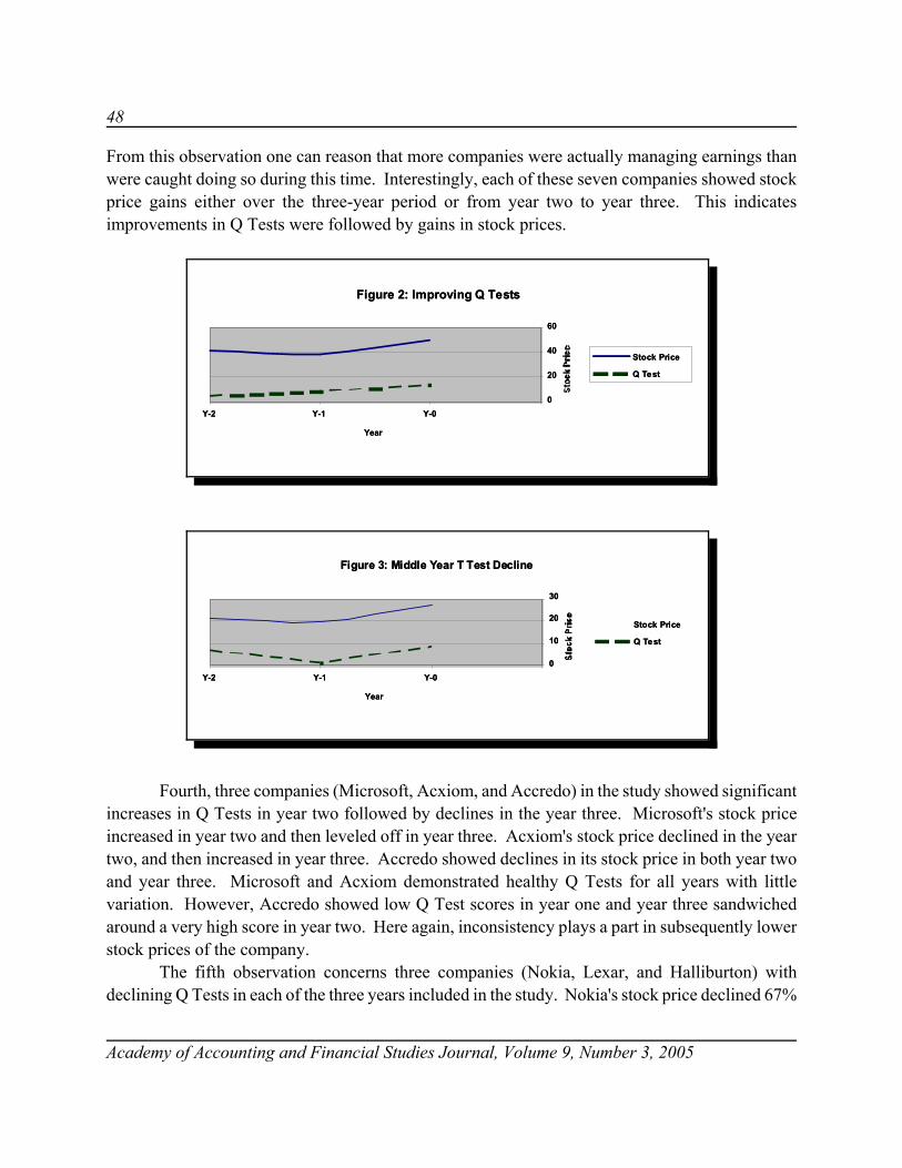
48


From this observation one can reason that more companies were actually managing earnings thanwere caught doing so during this time. Interestingly, each of these seven companies showed stockprice gains either over the three-year period or from year two to year three. This indicatesimprovements in Q Tests were followed by gains in stock prices.

Fourth, three companies (Microsoft, Acxiom, and Accredo) in the study showed significantincreases in Q Tests in year two followed by declines in the year three. Microsoft's stock priceincreased in year two and then leveled off in year three. Acxiom's stock price declined in the yeartwo, and then increased in year three. Accredo showed declines in its stock price in both year twoand year three. Microsoft and Acxiom demonstrated healthy Q Tests for all years with littlevariation. However, Accredo showed low Q Test scores in year one and year three sandwichedaround a very high score in year two. Here again, inconsistency plays a part in subsequently lowerstock prices of the company.

The fifth observation concerns three companies (Nokia, Lexar, and Halliburton) withdeclining Q Tests in each of the three years included in the study. Nokia's stock price declined 67%

Figure 2: Improving Q Tests

0

20

40

60

Y-2 Y-1 Y-0

Year

Stock Price

Q Test

Figure 2: Improving Q Tests

0

20

40

60

Y-2 Y-1 Y-0

Year

Stock Price

Q Test

Figure 3: Middle Year T Test Decline

0

10

20

30

Y-2 Y-1 Y-0

Year

Stock Price

Q Test

Figure 3: Middle Year T Test Decline

0

10

20

30

Y-2 Y-1 Y-0

Year

Stock Price

Q Test

49


in year two, and then rebounded for a 45% gain in year three. Nokia's Q Test scores, even thoughthey declined in each year, remained double digit healthy. This probably accounts for Nokia'sability to rebound to previous stock price levels in year three. Lexar's Q Tests gyrated from 3.28 inyear one to 16.56 in year two and back to 4.98 in year three. The tremendous decline in its stockprice from year two to year three is indicative of problems with its quality of earnings. Halliburtonis another case for more intensive study. Stock prices increased by substantial amounts even thoughthe Q Tests declined each year in the series. This appears to be a case where media releases andother extraneous market factors trump quality of earnings as stock price drivers. Halliburton's wellpublicized involvement in the Afghanistan and Iraqi Wars appears to have met with favor amonginvestors.

Finally, something should be said about TyCo, International. TyCo's Q Test scores were lowtherefore indicative of low quality earnings for the three year period. The score declined from 2.63to .297 from year one to year two, and then increased to 1.43 in year three. However, its stock priceincreased rather nicely from $17.08 to $20.73 to $35.74 during the same time frame. Throughoutthe time the company received media attention for financial improprieties and other corporatemisappropriations, its stock price remained solid. The possible explanation for this phenomenoncould be TyCo's corporate strategy of diversification. TyCo's revelation of its corporate scandal tothe public, unlike that of Enron and WorldCom, did not impair its financial soundness. This allowedthem to weather a period of inferior quality earnings until they could get their house in order onceagain.

Results of research in this study endorse the following observations about Q Testmeasurements. First, anything below 5.0 indicates suspect quality of earnings. When one obtainsa measurement at this level, it should lead to further investigation of the company involved todetermine the quality of other reported financial information such as asset values and liabilities.Next, if the Q Test falls between 5.0 and 9.99, the financial analyst should accept the reportedearnings as better than average quality. Finally, any Q Test over 10.00 (double digit) indicatessuperior quality earnings and, therefore, reported earnings can be relied upon as indication of trueearnings and consequently true corporate growth.

CONCLUSION

The Q Test that we propose in this article should help analysts discriminate between qualityearnings and traditional bottom line earnings. Since earnings are primary stock price drivers and,accordingly, have been the object of various management schemes in recent years, it is importantto develop a test such as the one we propose to detect such schemes early. The Q Test should beused to determine quality of reported earnings and not as a predictor of overall stock pricemovement. It is merely a tool that one can use to help evaluate investment potential of companystock. Other intangible factors such as general market movement, economic trends, and media

50


releases should continue to play important roles in investment strategies along with the Q Testanalysis proposed in this article.

REFERENCES

Amernic, Joel H., and Sean Robb (2003). ‘Quality of earnings’ as a framing device and unifying theme in IntermediateFinancial Accounting. Issues in Accounting Education. 18(1), February, 7-9.

Branner, Laurie (2001). Auditor independence and earnings quality. Business Finance, December 7, 12.

Brown, Paul R. (1999). Earnings management: A subtle (and troublesome) twist to earnings quality. Journal of FinancialStatement Analysis, Winter, 4(2), 61-63.

Eidleman, Gregory J. (1995). Z scores – a guide to failure prediction. The CPA Journal on Line. Retrieved February 15,2005, from http://www.nysscpa.org/cpajournal/old/16641866.htm

Krantz, Matt. (2002). Avoiding the next Enron: ‘Low Quality’ earnings can be helpful warning signs for investors. USAToday, February 1.

Largay, III, James A. and Clyde P. Stickney (1980). Cash flows, Ratio analysis and the W. T. Grant bankruptcy.Financial Analysts Journal, July-August, 78-82.

McClure, Ben (2004). Quality earnings count. Investing. March 11. Retrieved February 21, 2005, fromhttp://www.fool.com/news/commentary/2004/commentary040311ben.htm

Mills, J.R. and J.H. Yamamura (1998). The power of cash flow ratios. Journal of Accountancy, March. 53-61.

Morgenson, Gretchen. (1999). Taking the shine off Lucent earnings. New York Times-Market Watch, April 11.

Stickney, Clyde P., Paul R. Brown, and James M. Wahlen (2004). Financial Reporting and Statement Analysis, 2e. 157-167, 344.

Wayman, Rick. (2003). How to evaluate the “Quality” of EPS. Investopedia. September 19. Retrieved February 21,2005, from http://www.investopedia.com/articles/ analyst/03/091703.asp

51


INVESTOR RISK AVERSION AND THE WEEKENDEFFECT: THE BASICS

Michael T. Young, Minnesota State University - Mankato

ABSTRACT

This paper provides an explanation of the continued persistence of the weekend effect. Usingthe 23 non-holiday Wednesday closings of 1968 as a benchmark, it is postulated that negativeMonday returns can be explained by risk averse investors reacting to the arrival of new information.

INTRODUCTION

It is well documented that stock returns, on average, are statistically lower on Monday. Yetthere is little consensus on the explanations for this phenomenon. This paper pursues twoobjectives. First, to provide additional theoretical insight into the empirical persistence of theweekend effect, and secondly, using the non-holiday Wednesday closings of 1968, examine theunderlying liquidity and information dissemination processes and thereby isolate factors driving theweekend effect. Of particular interest is the employment of pre-1986 daily liquidity and informationdata from the Center of Research in Security Prices (CRSP).

During the second half of 1968, the NYSE and the AMEX were closed on twenty-threeWednesdays due to a backlog of paperwork. These closings offer a unique opportunity to analyzethe anomalous behavior of the market surrounding non-trading hours. By using cross-sectional datathis study observes several determinants of information flow and market liquidity related toindividual security prices.

An opportunity to test the effect of information flow on anomalous returns is provided bythe systematic discontinuities in trading surrounding the 1968 Wednesday closings. Thetwenty-three closed Wednesdays were non-trading, regular business days with full information flowin the market, whereas weekends represent non-trading, non-business days with reduced informationflow.

LITERATURE

Differences in information processing are usually explained using three different hypotheses,(French & Roll, 1986). First, public information is more likely to arrive during normal businesshours. Second, private information affects prices throughout the trading day. Third, noise caused

52


by trading may induce pricing errors. In light of these three hypotheses, the 1968 Wednesdayclosings represent normal business days when no information, public or private, can be absorbedinto the market. While weekends are non-trading days with information absorption into the marketnot being possible, they are also non-business days with less information flow available forabsorption. Weekends are non-trading, non-business days, whereas the twenty-three closedWednesdays are non-trading, regular business days. Also, interestingly, for the 1968 closedWednesdays, there is no trading noise to induce pricing errors.

The major component of liquidity reflected in market data, and addressed in this study isdaily volume. (Karpov, 1987) provides a comprehensive review of the work related to theprice/volume relationship through 1986. Most studies find a positive correlation between pricechange and volume. Other studies look at the NYSE intraday bid-ask spread as a measure ofvolatility. (Keim & Stambaugh, 1984) hypothesize, test, and reject the hypothesis that marketmakers transacting at the bid (ask) price with disproportionate frequency at the market close oncertain days of the week could induce low (high) returns on those days. They indicate that bid-askeffects can be discounted as an important contributor to high pre-holiday returns. However,holidays, while representing non-trading days, often represent non-business days. Holidays, beingnon-business days, do not have the same information flows as do the non-trading, regular businessclosed Wednesdays of 1968. (Stoll & Whaley, 1990) propose that wider spreads reflect thespecialists' ability to profit from their privileged knowledge. (Brock & Kleidon, 1992) testspecialists' monopoly power to control inelastic demand during times of wider spread. (Madhavan,1992) explains wider spreads with variation in the cost of adverse selection. (Lee, Mucklow &Ready, 1993) document the relationship between the intraday width of bid-ask spreads for NYSEstocks and reported earnings, which reflects information flow occurring only on business days.Further evidence of a day-of-the-week effect for bid-ask spreads is provided by (Chordia, Roll &Subrahmanyam, 2001). These authors find that, for a sample of NYSE stocks, liquidity declineson Friday and spreads increase "dramatically" during down markets but decline only slightly duringup markets.

A conclusive body of literature demonstrates that seasonal return patterns for equitysecurities vary by firm size. (Rogalski, 1984) finds significant differences in post-holiday return byweekday and firm size. (French, 1980) uses a time-diffusion process as an explanation for higherthan expected returns for post-holiday trading days for every weekday except Tuesday. (Roll, 1983)finds high returns accruing to small firms on the trading day prior to New Year's Day. (Lakonishok& Smidt, 1984) note that “prices also rise in all (size) deciles (of market capitalization) on the lasttrading day before Christmas.” (Merrill, 1965) finds a disproportionate frequency of Dow JonesIndustrial Average advances on days preceding holidays during the 1897 to 1965 period. (Keim &Stambaugh, 1984) indicate that the weekend effects generate significant premiums that accrue tosmall firms on Fridays.

53


Some research incorporates the 1968 Wednesday closings and/or the weekend effect involume and volatility studies. (French & Roll, 1986) and others show that returns are more volatileduring exchange trading hours than during non-trading hours. In addition, French and Roll arguethat private information dissemination is the principle factor behind high trading-time variances.(Jain & Joh, 1988) report that average volume across the days of the week (and for each hour) aresignificantly different. Average daily trading volume is lowest on Monday, increases from Mondayto Wednesday, and then declines on Thursday and Friday. (Ross, 1989) argues that “in anarbitrage-free economy, the volatility of prices is directly related to the rate of flow of informationto the market.” (Pettengill, 1989) tests whether the weekend effect is a closed market effect byexamining the difference between the mean returns on the trading days prior to exchange holidaysand on ordinary days. He finds no significant difference between Wednesday closings and regulartrading days. However, Pentengill's study excludes the trading days immediately adjacent to thetwenty-three 1968 closed Wednesdays. (Houston & Ryngaert, 1992) look at volume and volatilitypatterns for weeks with Wednesday closings. They report that Wednesday closings did not affectweekly volume or weekly volatility. However, they argue that volume and variance are shiftedbetween periods within the weeks with reduced trading hours. This is consistent with reducedtrading, temporarily and simultaneously, reducing the transmission of private information into tradedmarket prices. They further indicate that trading volume is redistributed rather evenly amongMonday, Tuesday, and Friday with the largest increase in trading volume on Thursday followingWednesday closings. Trading volatility is also redistributed to the remaining four days with thelargest increase on Fridays and smallest on Mondays. (Steeley, 2001) finds that a day-of-the-weekeffect exists for market returns in the UK and is related to the arrival time and nature of newinformation. Finally, (Berument & Halil, 2001) report that the variance of the S&P 500 index is afunction of the week day. They find that variance is highest on Friday and lowest on Wednesdayand propose that Friday's high variance is the result of increased levels of macroeconomic newsreleases on Thursday and Friday. Although some of these works include an examination of the 1968Wednesday closings, none provide a tested explanatory link between non-trading, regular businessday influences and liquidity and information flow. This can be attributed in part to the, heretofore,unavailable necessary data.

PREMISE

Stock returns on Monday are lower than other days. Why? There is no clear consensus.With a cursory review, there appears to be no consistent and logical reason for Monday to be anydifferent than other days except for the fact that the market is closed over the weekend. However,market closure in and of itself should make no difference. The premise here is that if the market isclosed, and there is no new information arriving, then the price should not change. If there is newinformation while the market is closed, then the market should react in the following ways:

54


1) Good News: The spread should increase slightly as analysts try to determine the new “correct” price. Ifnothing else, the Ask price should increase. The volume should also go up as traders try to react to theinformation. Return should increase as investors react to the news.

2) Bad News: The market reaction should be the same as above but in the opposite direction for the spread.Volume should go up as investors try to dump the stock. Finally, returns should decrease for obvious reasons.

3) Ambiguous Information: The spread should increase substantially while analysts try to assess the impacton firm price. Volume should increase substantially as some traders believe the information to be good andothers believe it to be bad and try to make a profit by trading accordingly. If investors are risk neutral, the pricewill remain unchanged provided the information is truly ambiguous as the number of traders who believe theprice will increase and those that believe that it will decrease should be the same. However, if participants inthe market are risk averse, they will be more inclined to attempt to protect themselves from loss rather thanattempt to profit on the information thus causing a decrease, or at a minimum no change, in price.

The preceding premise is dependent on the stock being actively traded. If the stock is heldin a portfolio primarily as a “buy-and-hold” security, the market reactions will be somewhatmitigated. This is often the case for large firms. In addition, the larger the firm, the larger thenumber of analysts who follow the stock, thereby increasing the likelihood of the market reachinga consensus on the “correct” new price prior to the market opening, thus reducing the premiseeffects. This will not necessarily hold true for securities of smaller firms, indicating that small andlarge firms should be viewed differently in light of return, liquidity, and information flows.

Even with a conservative assumption that there are equal amounts of good, bad, andambiguous information coming to the market after closure on Friday and over the weekend, oneshould see a low return, increased volatility, and increased liquidity (volume) on Monday. Asindicated earlier, a preponderance of past research supports this conclusion.

Therefore, if the arrival of information is the driving factor for Monday returns, then thereshould be the same effects on Thursday after a Wednesday close. In fact, the“closed-Wednesday-Thursday effect” should be more pronounced since there is informationdissemination of a full, active business day.

DATA AND METHODOLOGY

The hypothesis is that differences in daily returns can be explained by liquidity andinformation flow. Inferences are made using daily firm-specific data drawn from the Center ofResearch in Security Prices (CRSP) files. This approach is particularly appealing in that dailyliquidity and information data from periods prior to 1986, not available from CRSP before July1995, and therefore not available to most previous researchers, are used to provide empirical insightinto the persistence of the weekend effect.

To this end, this research investigates firm-specific daily returns, firm-specific tradingliquidity, and firm-specific trading information flow for firms whose stock was continuously traded

55


on the NYSE and/or the AMEX from the beginning of 1968 to the middle of 1969. The ability toattribute differences in volume and volatility to firm-specific rather than institutional factors isenhanced by the inclusion, not only of the NYSE firms, but of AMEX firms as well.

The applied methodology addresses the return-liquidity-information issue with a twoapproach process. In Approach I, ordinary least squares (OLS) analysis is performed for thetest-period, consisting of the twenty-three weeks with closed Wednesdays in 1968, and addressesreturn, dispersion, and volume differences between days of the week with particular attention givento Thursdays that follow closed Wednesdays. More complicated, alternative approaches for dailyreturns is offered by (Scholes & Williams, 1977) and (Dimson, 1979) that reduce the bias in theestimated b's, however, according to (Peterson, 1989), they do not provide a clear-cut benefit overOLS procedures. (Ingram & Ingram, 1993) indicate that joint generalized least squares (JGLS)methods have advantages over OLS procedure if there is significant cross-correlation. In this studycross-correlation is not found to be significant. Approach II addresses differences between days ofthe week for return, dispersion, and volume measures tested over two time periods:

1) Before-Closings: the pre-test period (January 1968 through June 1968)2) During-Closings: the test-period (the twenty-three weeks with closed Wednesdays in 1968); and

across two firm groups:1) Small Firms: Decile 1, the lowest capitalized firms, and2) Large Firms: Decile 10, the highest capitalized firms.

A traditional restrictive model approach is used that differentiates firm-specific daily returns,liquidity influences, and information flow influences by the day of the week for the test-period. Thisapproach differentiates firm-specific daily returns by the day of the week and isolates the impact ofliquidity and information influences. The following traditional restricted models for the four-daytrading week are applied to the firm-specific daily data for the twenty-three weeks with Wednesdayclosings:

Rt = b0 + b1D1t + b2D2t + b3D4t + ,t, (1)It = b0 + b1D1t + b2D2t + b3D4t + ,t, (2)Lt = b0 + b1D1t + b2D2t + b3D4t + ,t, (3)

where, Rt = the daily return, It = information flow (volatility measure) for the security, quantified by firm-specific relative

range: = daily high less the daily low / [(daily high plus the daily low)/2]

Lt = liquidity (volume measure) for the security, quantified by firm-specific relative volume:= the daily number of shares traded / the total number of shares outstanding

D1t = 1 if Monday, 0 otherwiseD2t = 1 if Tuesday, 0 otherwise D4t = 1 if Thursday, 0 otherwise ,i = disturbance term.

56


Previous research and a priori expectations indicate that in equation 1, b1 and b3 should benegative and the latter should have greater magnitude. If the hypothesis presented is correct, theselower returns on Monday and Thursday (after a Wednesday close) are a function of the arrival ofnew information. Therefore, in equations 2 and 3, b1 and b3 should be positive. Also, if a regularbusiness day produces more information than appears on the weekend, the latter should have greatermagnitude.

For the purpose of detecting the impact of liquidity and information flow on security returns,the usual, straight-forward method for testing the equality of means from two samples is employed.Typical t-test methodology is used to compare:

1) Daily information flow differences between the Before-Closings Period and the During-Closings Period for:a) Small and Large Firms together,b) Small Firms, andc) Large Firms;

2) Daily liquidity differences between the Before-Closings Period and the During-Closings Period for:a) Small and Large Firms together,b) Small Firms only, andc) Large Firms.

The usual t statistic for testing the equality of means is employed for the two samplecomparisons:

,)11()(

212

21

nnsxxt+

−=

where, s2 is the pooled variance

,2])1()1[(

21

222

2112

−+−+−

=nn

snsns

and, where s12 and s22 are the sample variances of the two groups. The usual assumption of equalpopulation variances for this t statistic in comparisons is satisfied.

Of particular interest is the intriguing polar contrast of decile sampling techniques. Byexamining the highest and lowest capitalized firms, decile sampling provides a polar analysis of theexistence of influential effects on liquidity and information predicated on firm size. Rather thanusing a firm size continuum, a more rigorous examination is made by comparing the extreme polesof firm size, namely the Small Firms and Large Firms groups.

In general, the information arrival should be the same in both the before-closings andduring-closings periods for all days except Thursday. Also liquidity should be higher on all dayswith Thursday getting the lion's share of the increases. This corresponds to the work done by(Houston & Ryngaert, 1992).

57


RESULTS

The first step in the analysis is to ascertain the pattern of returns, information arrival, andliquidity within the week. Parameter estimates from equation 1 appear in Table 1. As predicted,Thursday's returns are significantly less than Friday's for all three groupings. Also, the returns forthe large firm portfolio on Monday and Tuesday are less than Friday's return, but the decrease isonly one fourth that observed on Thursday. Of more interest, however, are the liquidity (equation2) and information flow (equation 3) results in Tables 2 and 3 respectively. Liquidity is significantlygreater on Thursday than any other day. In conjunction with this, information flow is greatest forall three portfolios on Thursday and for the combined and small firm portfolios on Monday. Themagnitude, as predicted, is greatest on Thursday.

Table 1: OLS Results For Testing Differences in Daily ReturnsIndependent Variable Combined Small-Firm Large-FirmIntercept (Friday) 0.001967** 0.003212** 0.000839** (0.0001) (0.0001) (0.0003)b1 (Monday) -0.000142 0.000416 -0.000648* (0.7330) (0.5999) (0.0493)b2 (Tuesday) -0.000801 -0.000964 -0.000654* (0.0537) (0.2240) (0.0473)b3 (Thursday) -0.002073** -0.001558* -0.002541**(0.0001) (0.0496) (0.0001)* significant at the 5% level** significant at the 1% levelParameter estimates for model: Rt = b0 + b1D1t + b2D2t + b3D4t + t, applied to the firm-specific daily data forthe twenty-three weeks in 1968 with Wednesday closings. Where, Rt is the average daily return. The Combinedportfolio consists of all firms whose stock was continuously traded on the NYSE and/or AMEX from thebeginning of 1968 through the middle of 1969. The Small-Firm and Large-Firm portfolios consist of the smallestand largest capitalization decile respectively.

Having identified the fact that returns are lower on Monday and Thursday, that informationflow is larger on these days, and that liquidity is greater on Thursday, the next step is to determineif there is a change in these variables as a result of the Wednesday closings. The t-test results fora change in information flow for the three portfolios appear in Tables 4, 5, and 6. Information flowis numerically larger on all days except Thursday for all three portfolios during the before-closingsperiod. This difference is statistically significant only for the combined portfolio and the large firmportfolio, however. In contrast, the information flow is significantly greater during the after-closingsperiod on Thursday for all three portfolios. This result at first was rather surprising. However,assuming that there is no increase in information on any day during a Wednesday-closings week

58


except Thursday and observing that liquidity across all days has either remained constant orincreased, this result makes perfect sense. Holding all else constant, an increase in liquidity shouldcause the relative range (information flow) to decline. This simply puts the Thursday increases instark contrast and shows that the open business day generates a large amount of information thatmust be analyzed and absorbed into the market.

Table 2: OLS Results For Testing Differences in Daily LiquidityIndependent Variable Combined Small-Firms Large-FirmsIntercept (Friday) 0.003083** 0.005557** 0.000844** (0.0001) (0.0001) (0.0001)b1 (Monday) -0.000066 -0.000087 -0.000050 (0.5920) (0.7259) (0.1101)b2 (Tuesday) -0.000023 -0.000029 -0.000018 (0.8525) (0.9071) (0.5588)b3 (Thursday) 0.000472** 0.000715** 0.000251**(0.0001) (0.0040) (0.001)* significant at the 5% level** significant at the 1% levelParameter estimates for model: Lt = b0 + b1D1t + b2D2t + b3D4t + t, applied to the firm-specific daily data forthe twenty-three weeks in 1968 with Wednesday closings. Where, Lt is firm-specific daily relative volume. TheCombined portfolio consists of all firms whose stock was continuously traded on the NYSE and/or AMEX fromthe beginning of 1968 through the middle of 1969. The Small-Firm and Large-Firm portfolios consist of thesmallest and largest capitalization decile respectively.

A comparison of liquidity between periods shows an increase across all days for thecombined portfolio (Table 7) and the small firm portfolio (Table 8) with the largest increasesoccurring on Thursday. Relative daily trading volume for the combined portfolio increases by16.2% on Monday, 16.7% on Tuesday, and 23.1% on Friday. Thursday's increase is a staggering36.0%. As can be seen below, the small firms in the portfolio are driving these increases. The netresult is an overall weekly volume that is relatively unchanged. These numbers are consistent withthose of (Houston & Ryngaert, 1992). Thursday's increase is probably due to the markets' reactionto Wednesday's information as well as a general redistribution in trading patterns as investors makeup for lost time.

The small firm portfolio reflects a similar pattern of increases. Volume on Monday andTuesday increases by 19.9% and 20.4% respectively. Friday sees an increase of 27.6% andThursday nearly doubles that of Monday and Tuesday at 38.7%. It appears that for small firms,which are followed by fewer analysts, it takes two days to sort out the meaning of any informationwhich arrived on Wednesday.

59


Table 3: OLS Results For Testing Differences in Daily Information FlowIndependent Variable Combined Small- Firms Large-FirmsIntercept (Friday) 0.026336** 0.035244** 0.018270**(0.0001) (0.0001) (0.0001)b1 (Monday) 0.001225** 0.002082** 0.000440 (0.0002) (0.0005) (0.0552)b2 (Tuesday) 0.000318 0.000657 0.000008 (0.3409) (0.2691) (0.9698)b3 (Thursday) 0.003333** 0.003898** 0.002817** (0.0001) (0.0001) (0.0001)* significant at the 5% level** significant at the 1% levelParameter estimates for model: It = b0 + b1D1t + b2D2t + b3D4t + t, applied to the firm-specific daily data forthe twenty-three weeks in 1968 with Wednesday closings. Where, It is firm-specific daily relative trading range. The Combined portfolio consists of all firms whose stock was continuously traded on the NYSE and/or AMEXfrom the beginning of 1968 through the middle of 1969. The Small-Firm and Large-Firm portfolios consist of thesmallest and largest capitalization decile respectively.

Table 4: T-Test Comparing Daily Information Flow Before and During Wednesday Closings:Combined Portfolio

Day of the Week Monday Tuesday Thursday FridayMean Before Closings 0.02859637 0.02746306 0.02839674 0.02728663Mean After Closings 0.02756052 0.02665362 0.02955900 0.02215075Prob > |T| 0.0025 0.0137 0.0003 0.0037Information flow is measured as the firm-specific daily relative trading range. The Combined portfolio consistsof all firms whose stock was continuously traded on the NYSE and/or AMEX from the beginning of 1968through the middle of 1969.

Table 5: T-Test Comparing Daily Information Flow Before and During Wednesday Closings: Small-FirmDay of the Week Monday Tuesday Thursday FridayMean Before Closings 0.03736189 0.03616932 0.03703348 0.03586639Mean After Closings 0.03732636 0.03590122 0.03914173 0.03524393Prob > |T| 0.9544 0.6526 0.0009 0.2942Information flow is measured as the firm-specific daily relative trading range. The small-firm portfolio consistsof the smallest capitalization decile of all firms whose stock was continuously traded on the NYSE and/or AMEXfrom the beginning of 1968 through the middle of 1969.

60


Table 6: T-Test Comparing Daily Information Flow Before and During Wednesday Closings: Large-FirmDay of the Week Monday Tuesday Thursday FridayMean Before Closings 0.02061107 0.01953222 0.02052350 0.01947363Mean After Closings 0.01871067 0.01827890 0.02108688 0.01827019Prob > |T| 0.0000 0.0000 0.0248 0.0000Information flow is measured as the firm-specific daily relative trading range. The large-firm portfolio consists ofthe largest capitalization decile of all firms whose stock was continuously traded on the NYSE and/or AMEXfrom the beginning of 1968 through the middle of 1969.

Table 7: T-Test Comparing Daily Liquidity Before and During Wednesday Closings: Combined PortfolioDay of the Week Monday Tuesday Thursday FridayMean Before Closings 0.00259552 0.00262157 0.00261368 0.00250412Mean After Closings 0.00301673 0.00306026 0.00355552 0.00308338Prob > |T| 0.0000 0.0000 0.0001 0.0001Liquidity is measured as the firm-specific relative daily volume. The Combined portfolio consists of all firmswhose stock was continuously traded on the NYSE and/or AMEX from the beginning of 1968 through the middleof 1969.

Table 8: T-Test Comparing Daily Liquidity Before and During Wednesday Closings: Small-FirmDay of the Week Monday Tuesday Thursday FridayMean Before Closings 0.00456254 0.00459088 0.00452039 0.00435591Mean After Closings 0.00547016 0.00552826 0.00627191 0.00555727Prob > |T| 0.0000 0.0000 0.0001 0.0001Liquidity is measured as the firm-specific relative daily volume. The small-firm portfolio consists of the smallestcapitalization decile of all firms whose stock was continuously traded on the NYSE and/or AMEX from thebeginning of 1968 through the middle of 1969.

Table 9: T-Test Comparing Daily Liquidity Before and During Wednesday Closings: Large-FirmDay of the Week Monday Tuesday Thursday FridayMean Before Closings 0.00080359 0.00082766 0.00087552 0.00081783Mean After Closings 0.00079342 0.00082521 0.00109452 0.00084355Prob > |T| 0.7020 0.9288 0.0001 0.3514Liquidity is measured as the firm-specific relative daily volume. The large-firm portfolio consists of the largestcapitalization decile of all firms whose stock was continuously traded on the NYSE and/or AMEX from thebeginning of 1968 through the middle of 1969.

61


The large firm portfolio (Table 9) has no change in liquidity on any day except Thursdaywhich has a 25.0% increase. In fact, the relative volume decreased on Monday, Tuesday, andFriday, but these changes are not statistically significant. For those who believe in an efficientmarket this is good news. The more closely watched larger firms react very quickly to any newinformation.

SIGNIFICANT IMPLICATIONS

While previous studies fail to provide a consensus explanation for negative Monday returns,this study synthesizes a coherent explanation of “anomalous” Monday negative returns. The intentis to show that negative Monday returns are not anomalous, and can be explained logically basedupon the degree of liquidity and information flow.

The most important result is that on Thursday following a Wednesday market closing, returnsare significantly lower while information flow and liquidity are significantly larger. This indicatesthat when there is an increase in information coming to the market, traders, being risk averse, lowerthe price of securities until they can process the information and/or observe the markets' reaction.It is reasonable to assume, therefore, that this reaction is not limited only to days following a normalbusiness day with the market closed, but also on Mondays which follow information arrival over theweekend.

REFERENCES

Berument, Hakan & Halil Kiymaz (2001). The Day-of-the-Week Effect on Stock Market Volatility. Journal ofEconomics and Finance, 25, 181-193.

Brock, W. & A. Kleidon (1992). Periodic Market Closure and Trading Volume: A Model of Intraday Bids and Asks.Journal of Economic Dynamics and Control, 16, 451-489.

Chan, K. C., William G. Christie & Paul H. Schultz (1995). Market Structure and the Intraday Pattern of Bid-AskSpreads for NASDAQ Securities. Journal of Business, 68, 35-60.

Connolly, Robert A. (1989). An Examination of the Robustness of the Weekend Effect. Journal of Financial andQuantitative Analysis, 24, 133-168.

Chordia, Tarum, Richard Roll & Avanidhar Subrahmanyam (2001). Market Liquidity and Trading Activity. Journalof Finance, 56, 501-530.

Cross, Frank (1973). The Behavior of Stock Prices on Fridays and Mondays. Financial Analysis Journal, 29, 67-69.

Dimson, E. (1979). Risk Measurement When Shares are Subject to Infrequent Trading. Journal of FinancialEconomics, 7, 197-226.

62


Fama, Eugene (1965). The Behavior of Stock Market Prices. The Journal of Business, 38, 34-105.

French, Kenneth R. (1980). Stock Returns and the Weekend Effect. Journal of Financial Economics, 8, 55-69.

French, Kenneth R. & Richard Roll (1986). Stock Return Variances. Journal of Financial Economics, 17, 5-26.

Gibbons, Michael R. & Patrick Hess (1981). Day of the Week Effects and Asset Returns. Journal of Business, 54, 579-596.

Harris, Lawrence (1986). A Transaction Data Study of Weekly and Intradaily Patterns in Stock Returns. Journal ofFinancial Economics, 16, 99-118.

Houston, Joel F. & Michael D. Ryngaert (1992). The Links Between Trading Time and Market Volatility. The Journalof Financial Research, 15, 91-100.

Ingram, Marcus A. & Virginia C. Ingram (1993). Consistent Estimation of Residual Variance in Regulatory EventStudies. The Journal of Financial Research, 16, 151-161.

Jain, P. & G. Joh (1988). The Dependence Between Hourly Prices and Trading Volume. Journal of Financial andQuantitative Analysis, 23, 269-283.

Karpov, J.M. (1987). The Relation Between Price Changes and Trading Volume: A Survey. Journal of Financial andQuantitative Analysis, 22, 109-126.

Keim, Donald B. & Robert F. Stambaugh (1984). A Further Investigation of the Weekend Effect in Stock Returns.Journal of Finance, 39, 819-835.

Lakoniskok, Josef & Maurice D. Levi (1982). Weekend Effects on Stock Returns: A Note. Journal of Finance, 37, 883-889.

Lakoniskok, Josef & Seymour Smidt. (1984). Volume and Turn-of-the-Year Behavior. Journal of Financial Economics,13, 435-456.

Lee, C., B. Mucklow & M. Ready (1993). Spreads, Depths, and the Impact of Earnings Information: An IntradayAnalysis. Review of Financial Studies, 6, 345-374.

Madhaven, A. (1992). Trading Mechanisms in Securities Markets. Journal of Finance, 47, 607-641.

Madhavan, A. & S. Smidt (1993). An Analysis of Changes in Specialist Inventories, and Quotations. Journal ofFinance, 48, 1595-1628.

Merrill, Arthur A. (1965). Year-End Rally; The Holiday Eves Especially Favor the Bulls. Barron’s, 45, 9.

Oldfield, George S. & Richard J. Rogalski (1980). A Theory of Common Stock Returns Over Trading and Non-TradingPeriods. Journal of Finance, 35, 729-752.

63


Penman, Stephen H. (1987). The Distribution of Earnings News over Time and Seasonalities in Aggregate StockReturns. Journal of Financial Economics, 18, 199-228.

Peterson, Pamela P. (1989). Event Studies: A Review of Issues and Methodology. Quarterly Journal of Business andEconomics, 28, 36-66.

Pettengill, Glenn N. (1989). Holiday Closings and Security Returns. Journal of Financial Research, 12, 57-67.

Rogaliski, Richard J. (1984). New Findings Regarding Day of the Week Returns over Trading and Non-TradingPeriods: A Note. Journal of Finance, 39, 1603-1614.

Roll, Richard (1983). On Computing Mean Returns and the Small Firm Premium. Journal of Financial Economics, 12,371-387.

Ross, Stephen A. (1989). Information and Volatility: The No-Arbitrage Martingale Approach to Timing and ResolutionIrrelevancy. Journal of Finance, 44, 1-17.

Scholes, Myron & Joseph Williams (1977). Estimating Betas From Nonsynchronous Data. Journal of FinancialEconomics, 5, 309-327.

Smirlock, Michael J. & Laura Starks (1987). Day-of-the-Week and Intraday Effects and Risk Measurement - AComment. Journal of Finance, 42, 181-187.

Steeley, James M. (2001). A Note on Information Seasonality and the Disappearance of the Weekend Effect in the UKStock Market. Journal of Banking and Finance, 25, 1941-1956.

Stoll, Hans R. & Robert E. Whaley (1990). Stock Market Structure and Volatility. Review of Financial Studies, 3, 37-71.

64


65


THE EFFECT OF THE FIRM'S MONOPOLY POWERON THE EARNINGS RESPONSE COEFFICIENT

Kyung Joo Lee, Cheju National UniversityJongdae Jin, University of Maryland-Eastern Shore

Sung K. Huh, California State University-San Bernardino

ABSTRACT

The purpose of this study is to provide further evidence on the determinants of the earningsresponse coefficient (ERC). More specifically, we have attempted to examine the ‘monopoly power'of a firm as an additional factor affecting the ERC. Using a firm valuation model that explicitly incorporates the degree of monopoly power in itsproduct markets (Thomadakis, 1976; Subrahmanyan and Thomadakis, 1980), we demonstrate thatthe ERC is positively related to the firm's monopoly power.

This theoretical prediction is empirically examined using a sample of 144 Korean firmslisted in the Korean Stock Exchange during the period extending from 1986 to 1992. The samplefirm's monopoly power is measured by whether or not the firm is designated as a market-dominantenterprise by the Korean Fair Trade Commission according to the Monopoly Regulation and FairTrade Act. Such designation implies that the firm has a monopoly power.

The empirical results are generally consistent with the theoretical prediction. Specifically,the ERC is higher for the designated firms than for the non-designated firms. This result is robustacross different methods.

INTRODUCTION

The determinant of cross-sectional and/or inter-temporal variations of the earnings responsecoefficient (hereafter, ERC in short) has been investigated in quite a few previous studies (e.g.,Kormendi and Lipe, 1987; Collins and Kothari, 1989; Easton and Zmijewski, 1989; Dhaliwal, Leeand Fargher, 1991; Dhaliwal and Reynolds, 1994; Ahmed, 1994; Kallapur, 1994; Choi and Jeter,1992; Biddle and Seow, 1991; Teets, 1992; Collins and Salatka, 1993; Bandyopadbyay, 1994). Thedeterminants of the ERC identified in previous studies are characteristics of the firm's earningsgenerating process, systematic risk of common stock, firm size, the default risk, growth opportunity,cost structure, dividend payout ratio, audit opinion, industry, and interest rates. However, the effectof a firm's monopoly power on the ERC has not been extensively investigated, so far. Thus, the

66


purpose of this study is to examine the effect of a firm's monopoly power on the ERC using Koreancapital market data.

Using a firm valuation model that explicitly incorporates the degree of monopoly power inits product markets (Thomadakis, 1976; Subrahmanyan and Thomadakis, 1980), we demonstrate thatthe ERC is positively related to the firm's monopoly power. This theoretical prediction is empiricallytested by comparing ERC's between the firms designated as market-dominant enterprises by theMonopoly Regulation and Fair Trade Act and the other firms. To the extent that designation as amarket-dominant enterprise is an appropriate proxy for the degree of monopoly power, we expectthe ERC's of the designated firms to be higher than those of the non-designated firms.

The remainder of this paper is organized as follows. In the next section, we derive thetheoretical relationship between the firm's monopoly power and the ERC within the framework ofa firm valuation model developed by Thomadakis (1976), Subrahmanyan and Thomadakis (1980),and Ahmed (1994). Section three contains our research hypothesis and research methodology.Section four describes sample selection procedure and descriptive statistics for the variables used.The empirical results are presented in section five. A summary of the results and some suggestionsfor future research appear in final section.

MONOPOLY POWER AND EARNINGS RESPONSE COEFFICIENT

A firm valuation model based on cash flow has been used in many previous ERC literaturesuch as Kormendi and Lipe (1987), Collins and Kothari (1989), Dhaliwal, Lee and Fargher (1991),and Dhaliwal and Reynolds (1994). On the other hand, Thomadakis (1976) and Subrahmanyan andThomadakis (1980) developed a model that incorporates the degree of monopoly power in thevaluation of a firm. By combining these two valuation approaches, we develop a valuation modelthat describes a functional relationship between the monopoly power and the ERC.To simplify the analysis, we make the following assumptions:

Assumption 1: The demand function faced by the firm is

nttt qap −=

Where p = the price of a unit of product in period t; q= the quantity of output chosen by a firm in period t; a= a random variable representing the uncertainty concerning the demand function. Its mean,

variance and covariance are constant through time; n = the measure of a firm's monopoly power, 0 # n # 1.

From Assumption 1, the marginal revenue (MR) is (1-n) aq-n and the average revenue (AR) is aq-n.Therefore, the firm is in a perfect competition when n=0 and hence MR=AR= p, while the firm is

67


in a monopolistic position when n>0. Also, since n is the inverse of the elasticity of demand, thedemand becomes more inelastic as n increases. Therefore, n is reliable measure of a firm's monopolypower. This is also evident from the fact that Lerner's index, a popular measure of the monopolypower, is usually defined as 1/(1-n).

Assumption 2: The cost function for the firm is

ttt qcTC =

Where TC= the total cost;c= the operating cost per unit of output in period t. c is invariant to the level of output, and its

mean, variance and covariance are also constant through time.

Assumption 3: As a discount rate for the capitalization of a firm's future cash flow, a singleperiod CAPM is applicable to each period. Also, it is assumed that the market parametersin the CAPM (risk-free rate, market returns, and systematic risk) are exogeneous andconstant through time. Thus, the risk-adjusted expected return for a firm in period t (Kt) is:

[ ]fmft RRERK −+= )(β

Where $ = the systematic risk of the firm;Rf = the risk-free interest rate;Rm = the rate of return on market portfolio

Using the above assumptions, a firm valuation model is developed in a two period world(Thomadakis, 1976). The firm's problem is to choose its output level that maximizes the presentvalue of its future cash flows. In a two period world, the sequence of events is as follows:

At the beginning of the first period (t=0), the firm chooses the optimal level of output (Q)for the first period based on expectation about future cash flows (i.e., prices and costs). Atthe end of the first period (t=1), prices and operating costs for the first period are realized.The firm revises its expectations about period 2 cash flows and chooses the optimal quantityfor period 2 based on the revised expectations. The firm is liquidated at the end of thesecond period. Under this setting, the firm's value at time 0 (V0) can be described as follow.

)1........()1)(1()(

1)(

21

22220

1

11110110 KK

QcQpnEK

QcQpnEQkV++−

++

−+=

68


Where pt = the price of a unit of product in period t; Qt = the quantity of output chosen by a firm in period t;Kt = the risk-adjusted expected return for a firm in period t;k1 = the actual risk-adjusted return for a firm in period 1;n = the measure of a firm's monopoly power, 0 # n # 1.

Abnormal returns or excess returns for the first period (AR1) are computed by the differencebetween realized returns (R1) and expected returns (ER1) as follows:

0

010

0

101111

)(V

VVEV

DVVERRAR −−

+−=−=

Where D1 = the dividend paid to stockholders after deducting investments for the second period from therealized cash flows in period one.

Two additional assumptions regarding the firm's earnings generating process are made todevelop a model for abnormal returns. First, cash flows to the firm and accounting earnings (Xt) areidentical (i.e., Xt = pt qt -ct qt ). Second, the firm's earnings have time-series characteristicsdescribed by the following model:

E1(X2) - E0(X2) = λ [X1 - E0(X1)]

Where 8 = the extent to which the current period's earnings shock affects the revisions in expectationsof future earnings, usually referred to as persistent coefficient. The sign and value of willdepend on the time-series properties of the firm's earnings.

It can be shown that 8 is a function of time-series model parameters even when earnings generatingprocess is specified by a general ARIMA(pdq) model (Collins and Kothari, 1989).

Then Abnormal returns or excess returns for the first period (AR1) can be described asfollow:

)2.........()(])([1

10

1011 V

XEXRRER

nARfmf

−

−+++=

βλ

It is obvious from equation (2) that the impact of $, 8, E(Rm)-Rf, and n on the ERC (the bracketterm) are, ceteris paribus:

0,0])([

,0,0 >∂

∂<

−∂∂

>∂

∂<

∂∂

nERC

RREERCERCERC

fmλβ

69


The first three results reveal that, if other factors be constant, the ERC is negatively relatedto both the systematic risk of the firm ($) and the market risk premium (E(Rm)-Rf), but positivelyrelated to the persistence coefficient (8). Previous studies such as Kormendi and Lipe (1987), Eastonand Zmizewski (1989), and Collins and Kothari (1989) provide empirical evidence consistent withthese predictions. The fourth comparative static result indicates that the ERC is a positive functionof the firm's monopoly power (n) in its product markets.

HYPOTHESIS AND RESEARCH DESIGN

Hypothesis

The research question addressed in this study is whether there is an association betweenfirm's monopoly power and the ERC. The analytical results in the preceding section suggest, amongother things, that the a firm's monopoly power is positively related to the ERC.

As a surrogate for the firm's monopoly power, the firm's designation as a market-dominantenterprise by the Monopoly Regulation and Fair Trade Act is used. According to the MonopolyRegulation and Fair Trade Act, the Korea Fair Trade Commission designates and notifiesmarket-dominant enterprises at the beginning of each year. A firm with its annual domestic salesexceeding 100 billion won is designated as a marker-dominant enterprise if its market share is over50% or 75% (combined with up to 3 other designated firms) in a same or similar industry. If a firmis designated as such, the firm (hereafter, designated firm) has a higher degree of monopoly powerrelative to other firms that are not designated (hereafter, non-designated firms).

A testable hypothesis for the positive relationship between the ERC and the firm's monopolypower derived herefrom would be,

Hypothesis: Earnings response coefficients of designated firms are higher than those of non-designated firms.

Measurement of Variables

Under an assumption that earnings are described by the random walk with a drift model.Expected earnings, E(X), can be written as follows:

tttt XXE δ+= −− 11 )(

Where Xt = the earnings at time t;* = a drift term obtained by averaging earnings changes for the 5 previous years.

70


Unexpected earnings (UE), excess of actual earnings over expected earnings, can bedescribed as follow:

1

1 )(

−

− +−=

it

itititit P

XXUE δ

Where Pit-1 = the market value of the equity of firm i at the beginning of period t (stock price times numberof shares outstanding).

Expected earnings as well as stock price are often used as a deflator. Stock price is chosenbecause it was shown to be a theoretically superior deflator (Christie (1987)) and has been used ina number of previous studies (e.g., Easton and Zmizewski (1989), Collins and Kothari (1989)). Toavoid the problem of extreme values, observations with |UE|>200% are truncated to 200%.

The systematic risk (BETA) of firm i in time t, is obtained by estimating the followingmarket model:

)3..(..........itjmtjitititj RR εβα ++=

Where Ritj = the rate of return on firm i during month j in year t;Rmtj = the rate of return on market portfolio during month j in year t;"it, $ it = the intercept and the slope coefficient, respectively, from the market model.

The above model is estimated using four years (48 months) of monthly return data up to 3months after the beginning of a fiscal year. If less than 24 monthly returns were available, thefirm-month observation is excluded from the analysis.

The estimated parameters, it and it, from the market model (3) are used to calculatemonthly abnormal returns (AR) as follows:

)( mtjitititjitj RRAR βα +−=

Where i = the firm index;t = the year index;j = the month index.

The monthly abnormal returns are then cumulated over twelve months up to the three monthsafter the end of the fiscal year to get cumulative abnormal returns (CAR):

∑=

=15

4jitjit ARCAR

71


Where CARit = the cumulative abnormal returns for firm i in year t;ARitj = the abnormal returns of firm i for the jth month of year t.

To test the hypothesis that ERC's of designated firms be higher than those of non-designatedfirms, we estimated the following regression model:

)4.(..........ititititit eUEDbUEaCAR +++= φ

Where UEit = the unexpected earnings for firm i in year t, Dit = the dummy variable which takes a value of one if firm i is designated as a

market-dominant enterprise ('designated firm') in year t, and zero if otherwise.

Test for any significant difference in ERC's between the designated firms and thenon-designated firms is equivalent to testing the significance of the estimated coefficient in theregression model (4). Thus, our hypothesis can be formally stated as:

Ho: N = 0, Ha: N > 0

SAMPLE SELECTION AND DESCRIPTIVE STATISTICS

The sample firms examined in this study are Korean firms listed on the Korean StockExchange as of December 31, 1992. To be included in the sample, the firm must satisfy thefollowing criteria: (1) Sufficient accounting data including net income and equity are available overthe study period (1981-1992); (2) Monthly security returns data are available from January 1981 toDecember 1992; (3) Firms in banking and finance industry are excluded. Criteria (1) and (2) areimposed to ensure the data availability of accounting earnings and returns data enough to carry outempirical analyses. The firms in banking and finance industry are excluded because they tend tohave different characteristics from the other firms. The above selection criteria yielded a sample of144 firms. The number of firms designated as market-dominant enterprises by the KFTC varies overtime. For example, 181 firms were designated in 1981 while 209 firms were designated in 1992.

The breakdown of sample firms by industry is shown in Table 1. The sample consists of 14industries and there are some clustering in particular industries. For example, designated firms infoods & beverage do have 29% market share, while those in textile industries have 14.5% marketshare. On the other hand, the medical products industry appears to be very competitive in the sensethat only 1 out of the total 17 sample firms is designated. In general, designated sample firms consistof large firms with a relatively long history and hence there may be a potential problem ofsurvivorship bias.

72


Table 1: Industry Classification of Sample Firms 1

Industry DesignatedFirms

Non-designatedFirms

TotalFirms

N % N % N %

Foods and Beverage 18 29.0 6 7.3 24 16.7

Textiles 9 14.5 11 13.4 20 13.8

Pulp, Paper and Paper Products 1 1.6 5 6.1 6 4.2

Chemicals & Chemical Products 6 9.7 11 13.4 17 11.8

Medical Products 1 1.6 16 19.5 17 11.8

Rubber Plastic Products 4 6.5 1 1.2 5 3.5

Non-metalic Mineral Products 5 8.1 9 11.0 14 9.7

Basic Metals 2 3.2 9 11.0 11 7.6

Fabricated Metal Products 1 1.6 4 4.9 5 3.5

Machinery and Equipment 5 8.1 1 1.2 6 4.2

Radio, TV and Communication Equipment 3 4.8 7 8.5 10 6.9

Electrical Machinery and Apparatus 3 4.8 0 0.0 3 2.1

Motor Vehicles and Trailers 3 4.8 2 2.5 5 3.5

Medical, Precision and Optical Instruments, Watches 1 11.6 0 0.0 1 0.7

Total 62 100.0 82 100.0 144 100.0

Table 2 provides descriptive statistics for selected variables of the sample firms. Alsoreported are Wilcoxon rank test statistics for the differences in these variables between designatedfirms and non-designated firms. Selected variables include unexpected earnings (UE), cumulativeabnormal returns (CAR), systematic risk (BETA), growth as measured by the ratio of market valueto book value of equity (GROWTH), leverage as measured by the ration of total liabilities to totalasset (LEVG), Tobin's Q ratio (QRATIO), return on asset (ROA), return on equity (ROE) and firmsize as measured by the market value of equity (SIZE).

As expected, the average firm size of the designated firms is much greater than that of thenon-designated firms: i.e., 2,366 billion Won for the designated firms ($1.57 billion at the exchangerate of 1500 Won per dollar as of August, 2004), while 528 billion Won ($0.35 billion) for thenon-designated firms. This difference is statistically significant at less than 0.01 confidence level.There is no significant difference in UE and CAR between the two groups. However, mean (median)systematic risk (BETA) of the designated firms is 0.816 (0.801), which is much smaller than thatof the non-designated firms. These differences are consistent with the theoretical prediction thatmonopoly power is negatively correlated with firm's systematic risk (Subrahmanyan andThomadakis, 1980).

73


Table 2: Descriptive Statistics of Selected VariablesVariable Designated Firms Non-designated Firms Wilcoxon

Z-value 11

Significance(p-value)

Mean S.D. Median Mean S.D. Median

UE 2 -0.001 0.131 0.001 -0.002 0.196 0.002 0.542 0.5871

CAR 3 0.061 0.362 0.058 0.057 0.424 0.045 0.535 0.5922

BETA4 0.816 0.239 0.801 0.936 0.282 0.935 -7.483 0.0001

GROWTH5 2.381 3.601 1.241 1.925 3.051 1.001 5.036 0.0001

LEVG 6 0.706 0.120 0.723 0.646 0.135 0.660 7.759 0.0001

QRATIO 7 1.356 0.945 1.051 1.268 0.884 1.000 4.557 0.0001

ROA 8 0.023 0.022 0.017 0.030 0.029 0.024 -4.334 0.0001

ROE 9 0.076 0.056 0.068 0.083 0.186 0.073 -1.072 0.2833

SIZE 10 236.59 558.53 75.24 52.78 84.90 26.59 12.519 0.0001

1) Total 1,064 observations were used for 144 sample firms during 7 years (1986-1992) 2) Cumulative abnormal returns are cumulated over 12 months form April to March of the year t + 13) Unexpected earnings as measured by subtracting expected earnings described by the random walk with driftmodel from actual earnings, and then deflated by total market value of equity at the beginning of the fiscal period.4) Systematic risk of common stock, estimated from market model.5) Growth as measured by the ratio of market value to book value of equity.6) Leverage as measured by the ratio of total liabilities to total assets.7) Tobin Q ratio = (Total Liabilities + Market value of equity) / Total assets8) Return on total assets = Net Income / Total Assets9) Return on equity = Net Income / Equity10) Firm size is measured by the market value of equity (10 billion won).11) Wilcoxon signed ranks tests statistics

The median ROA and ROE are statistically significantly greater for the non-designated firms,which appears to be contrary to our expectation from a monopoly gain perspective. On the otherhand, QRATIO of the designated firms are significantly greater than that of the non-designatedfirms. Higher QRATIO for the designated firms implies that the designation as a market dominantenterprise is recognized as having monopoly power in that product markets.

EMPIRICAL RESULTS

Table 3 presents the results from estimations of equation (4). We estimate equation (4) forthe designated firms and the non-designated firms, as well as total sample. The results are reportedfor two types of samples, one for the total sample (Sample A) and the other for the reduced-sample(Sample B) excluding those firms that changed their designation status. Overall results are consistentwith the theoretical prediction.

74


Table 3: Effects of Monopoly Power on the ERC

ititititit eUEDbUEaCAR +++= φ

Panel A: Sample A (including firms that changed their designation status)

Independent Variables Expected Sign Designated Firms Non-designatedFirms

Total Sample Firms

Intercept ? -0.177 ** (5.340) -0.142 ** (5.109) -0.156 ** (7.303)

UE + 1.159 ** (3.708) 0.408 * (2.397) 0.418 ** (2.510)

D*UE + 0.744 * (2.023)

R2 (%) 5.35 1.50 2.91

Panel B: Sample B (excluding firms that changed their designation status)


Total Sample Firms

Intercept ? -0.206 ** (5.599) -0.124 ** (4.144) -0.155 ** (7.303)

UE + 1.406 ** (2.473) 0.437 ** (2.400) 0.461 ** (2.510)

D*UE + 0.764 + (1.273)

R2 (%) 3.06 1.82 2.14

1) Dit is a dummy variable which takes a value of one if firm i for the year t belongs to designated firms, and zeroif firm i belongs to non-designated firms2) t-values are in parenthesis.+ : Significant at a = 0.10; * : Significant at a = 0.05; ** : Significant at a = 0.01.

Panel A of Table 3 shows the results for the total sample (Sample A). The ERC for thedesignated firms is 1.159, while that of non-designated firms is 0.408. The regression coefficient (N)of DitUEit in equation (4) are positive as predicted and statistically different from zero at thesignificance level of 0.05, supporting the Hypothesis.

Sample A may have some estimation bias because the number of the 'designated firms' is notsymmetrical with that of the 'non-designated firms' each year. Thus, we delete those firms thatchanged their designation status during the test period and hold only those firms that consistentlykeep designated or non-designated status over the whole test period. The results are shown in PanelB, which are quite consistent with the results in Panel A.

Overall, these results lend empirical support to our maintained hypothesis that the ERC isa positive function of a firm's monopoly power measured by the designation as a market dominantenterprise.

In general, the above results support our hypothesis. However, the empirical estimationprocedure might include the following potential problems. First, the firm size of the two samplegroups is significantly different from each other, which may contaminate the estimation results.Secondly, different industry distributions of the two groups may also contaminate the estimation

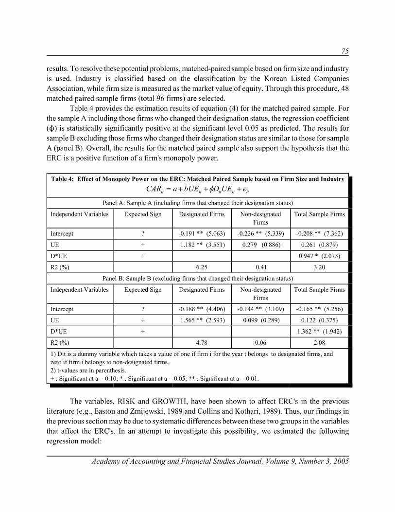
75


results. To resolve these potential problems, matched-paired sample based on firm size and industryis used. Industry is classified based on the classification by the Korean Listed CompaniesAssociation, while firm size is measured as the market value of equity. Through this procedure, 48matched paired sample firms (total 96 firms) are selected.

Table 4 provides the estimation results of equation (4) for the matched paired sample. Forthe sample A including those firms who changed their designation status, the regression coefficient(N) is statistically significantly positive at the significant level 0.05 as predicted. The results forsample B excluding those firms who changed their designation status are similar to those for sampleA (panel B). Overall, the results for the matched paired sample also support the hypothesis that theERC is a positive function of a firm's monopoly power.

Table 4: Effect of Monopoly Power on the ERC: Matched Paired Sample based on Firm Size and Industry

ititititit eUEDbUEaCAR +++= φ

Panel A: Sample A (including firms that changed their designation status)


Total Sample Firms

Intercept ? -0.191 ** (5.063) -0.226 ** (5.339) -0.208 ** (7.362)

UE + 1.182 ** (3.551) 0.279 (0.886) 0.261 (0.879)

D*UE + 0.947 * (2.073)

R2 (%) 6.25 0.41 3.20

Panel B: Sample B (excluding firms that changed their designation status)


Total Sample Firms

Intercept ? -0.188 ** (4.406) -0.144 ** (3.109) -0.165 ** (5.256)

UE + 1.565 ** (2.593) 0.099 (0.289) 0.122 (0.375)

D*UE + 1.362 ** (1.942)

R2 (%) 4.78 0.06 2.08

1) Dit is a dummy variable which takes a value of one if firm i for the year t belongs to designated firms, andzero if firm i belongs to non-designated firms.2) t-values are in parenthesis.+ : Significant at a = 0.10; * : Significant at a = 0.05; ** : Significant at a = 0.01.

The variables, RISK and GROWTH, have been shown to affect ERC's in the previousliterature (e.g., Easton and Zmijewski, 1989 and Collins and Kothari, 1989). Thus, our findings inthe previous section may be due to systematic differences between these two groups in the variablesthat affect the ERC's. In an attempt to investigate this possibility, we estimated the followingregression model:

76


)5........(*][ 3210 itititititit eUEDGROWbRISKbbbCAR +++++= φ

where RISKit = 1 if the systematic risk of common stock (BETA) for firm i in year t is above thesample median, and 0 if otherwise,

GROWit= 1 if growth rate (GROWTH) for firm i in year t is above the sample median, and 0if otherwise.

In equation (5), the coefficient b1 of UE is predicted to be positive as a measure ofusefulness of accounting earnings information. The b2 and b3 are predicted to be negative andpositive, respectively.

Table 5: Effect of Monopoly Power on the ERC: After controlling for Systematic Risk and Growth

itititititit eUEDGROWbRISKbbbCAR +++++= *][ 3210 φ

Total Sample

Independent Variables Expected Sign Sample A Sample B

Intercept ? -0.160 (7.469) ** -0.158 (6.796) **

UE + 0.723 (3.044) ** 0.866 (3.439) **

RISK*UE - -0.699 (2.107) * -0.853 (2.340) **

GROW*UE + 0.236 (0.617) 0.055 (0.138)

D*UE + 0.508 (1.308) + 0.589 (0.977)

R2 (%) 3.60 3.29

Matched Paired Sample

Independent Variables Expected Sign Sample A Sample B

Intercept ? -0.211 (7.514) ** -0.164 (5.217) **

UE + 0.834 (2.111) ** 0.581 (1.339) +

RISK*UE - -1.265 (2.453) ** -0.989 (1.667) *

GROW*UE + 2.468 (2.261) * 0.320 (0.231)

D*UE + 0.372 (0.747) 1.105 (1.538) +

R2 (%) 5.75 3.12

1) RISKit = 1 if the systematic risk of common stock for firm i in year t is above sample median, and 0 otherwise GROWit= 1 if growth (ratio of market value to book value of equity) for firm i in year t is above sample median,and 0 otherwise.2) t-value is in parenthesis+ Significant at a = 0.10; * Significant at a = 0.05; ** Significant at a = 0.0; all two tailed tests

77


Table 5 provides the empirical results for both total sample and matched paired sample. Eachsample includes two different groups: one group includes those firms that changed their designationstatus while the other group does not include those firms that changed their designation status.Overall, the coefficients on RISK and GROW have their predicted signs. Furthermore, thecoefficient b2 of RISK is statistically significant at the significance level of 0.05.

As expected, the estimate of the coefficient N on Dit*UEit are positive, which is similar toearlier results. The coefficients are statistically significant at the 0.10 significance level for sampleA of total sample and sample B of matched-paired sample.

CONCLUSIONS

The purpose of this paper is to provide further evidence on the factors that affect thecoefficient relating unexpected earnings and abnormal stock returns, viz., the ERC. In particular,this study examines whether a firm's monopoly power has a systematic impact on the ERC. Fromanalytical results, we derive a theoretical prediction that the ERC is a positive function of the firm'smonopoly power in its product markets.

Using a sample of 144 Korean firms listed in the Korean Stock Exchange during the periodfrom1986 to 1992, we empirically test this theoretical prediction. A firm's monopoly power ismeasured by whether or not the firm is designated as a market-dominant enterprise by the MonopolyRegulation and Fair Trade Act.

The empirical results are generally consistent with the theoretical prediction. Specifically,the ERC is higher for the designated firms than for the non-designated firms. This result is robustacross different methods and samples. The results from this study may provide additional insightsinto the effect of the monopoly power on the ERC and the economic effect of the monopolyregulation policy in Korea.

One related issues left for future research is a time-series approach that examines thedirection of changes in ERC's associated with shifts in the firm's monopoly power would providemeaningful results. For example, we can compare the ERC's over time using a sample of firms thatare newly designated as a market-dominant enterprise or de-listed from the designation.

REFERENCES

Ahmed, A. (1994). Accounting earnings and Future Economic Rents. Journal of Accounting and Economics, 377-400.

Ball, R. and P. Brown (Autumn 1968). An Empirical Evaluation of Accounting Income Numbers. Journal of AccountingResearch, 159-178.

Bandyopadhyay, S. (October 1994). Market Reaction to Earnings Announcements of Successful Efforts and Full CostFirms in the Oil and Gas Industry. Accounting Review, 657-674.

78


Biddle, G. and G. Seow (Spring 1991). The Estimation and Determinants of Association Between Returns and Earnings:Evidence from Cross-Industry Comparisons. Journal of Accounting, Auditing & Finance, 183-232.

Choi, S. and D. Jeter (June/Sept. 1992). The Effects of Qualified Audit Opinions on Earnings Response Coefficients,"Journal of Accounting & Economics, 229-247.

Christie, A. (December 1987). On Cross-sectional Analysis in Accounting Research. Journal of Accounting andEconomics, 231-258.

Collins, D. and S. Kothari (July 1989). An Analysis of Intertemporal and Cross-sectional Determinants of EarningsResponse Coefficients. Journal of Accounting and Economics, 143-181.

Collins, D. and W. Salatka (Fall 1993). Noisy Accounting Earnings Signals and Earnings response Coefficients: TheCase of Foreign Currency Accounting. Contemporary Accounting Research, 119-160.

Dhaliwal, D. and S. Reynolds (April 1994). The Effect of the Default Risk of Debt on the Earnings ResponseCoefficient. Accounting Review, 412-419.

Dhaliwal, D., K. Lee and N. Fargher (Fall 1991). The Association Between Unexpected Earnings and Abnormal SecurityReturns in the Presence of Financial Leverage. Contemporary Accounting Research, 20-41.

Easton, P. and M. Zmijewski (July 1989). Cross-sectional Variation in the Stock Market Response to AccountingEarnings Announcements. Journal of Accounting and Economics, 117-141.

Kallapur, S. (1994). Dividend Payout Ratios as Determinants of Earnings Response Coefficients. Journal of Accountingand Economics, 359-375.

Kormendi, R. and R. Lipe (July 1987). Earnings Innovations, Earnings Persistence, and Stock Returns. Journal ofBusiness, 323-345.

Subrahmanyan, M. and S. Thomadakis May 1980). Systematic Risk and the Theory of the Firm. Quarterly Journal ofEconomics, 437-451.

Thomadakis, S. (1976). A Model of Market Power, Valuation and the Firm's Returns. Bell Journal of Economics,150-162.

Teets, W. (Autumn 1992). The Association Between Stock Market Response to earnings Announcements and Regulationof Electric Utilities. Journal of Accounting Research, 274-285.

79


BRAND VALUE AND THE REPRESENTATIONALFAITHFULNESS OF BALANCE SHEETS

Philip Little, Western Carolina UniversityDavid Coffee, Western Carolina UniversityRoger Lirely, Western Carolina University

ABSTRACT

This study examines the impact of brand value on the representational faithfulness ofbalance sheets. The results of this research reveal that brand value is significant in explainingvariations in the price to book value ratios over and above the explanatory power of variables thatare typically thought to be related to price to book value differentials. These results suggest thatassets of firms with significant brand value may be underreported on the firms' balance sheets.Accordingly, if the representational faithfulness of balance sheets is to be enhanced, accountingstandards should consider including reliable measures of intangible assets (especially for highbrand value firms) in balance sheets.

BACKGROUND

Little and Coffee (2000) found that the balance sheets of knowledge and service basedcompanies are less representationally faithful than the balance sheets of more traditional firmsbecause they systematically under-report assets. They suggest that one reason for this may be thatthe assets of knowledge and service based companies include more soft, intangible assets as opposedto the comparatively hard, tangible assets of more traditional business enterprises like heavymanufacturing and traditional wholesaling/ retailing.

Knowledge and service based companies are not, however, the only kinds of companies thatmay have significant intangible assets. It is well established that brands like Nike, Coca-Cola,Disney and McDonald's are assets that have a separately identifiable economic value (Kallapur andKwan, 2004; Kerin and Sethuraman, 1998). Fernandez (2002) reports the Marketing ScienceInstitute definition of brand value as the "strong, sustainable, and differentiated advantage withrespect to competitors that leads to a higher volume or a higher margin for the company comparedwith the situation it would have without the brand." Interbrand (2001) estimates that brand valueaccounts for a significant percentage of the market value of the top 100 global brand companies.

The Financial Accounting Standards Board recognizes the potential economic value ofbrands with respect to intangibles acquired as part of a business combination. FASB Statement No.

80


141: Business Combinations (FAS 141), requires the use of the purchase method of accounting forbusiness combinations. Under this method, the acquiring company will be treated as though itpurchased the target company's net assets at their fair market value on the date of acquisition. Netpresent value is deemed to be the best method for determining fair market value. The use of thepurchase method requires that goodwill be recognized as an asset. Furthermore, other intangiblesshould be recognized as assets separate and apart from goodwill if these other intangibles either arisefrom contractual or legal rights or are capable of being transferred from the acquired entity. FAS141 in paragraph 16A identifies brand as a general marketing term typically used to refer to a groupof complementary assets such as the trademarks or service marks and their related trade names,formulas, recipes, and technological expertise which may or may not be patented. The statementdoes not preclude an entity from recognizing, as a single asset apart from goodwill, a group ofcomplementary intangible assets commonly referred to as a brand if the assets that make up thatgroup have similar useful lives.

Accordingly, brand value is not exclusive to knowledge and service based companies. Forthe last several years, Interbrand Corporation has estimated the value of the 100 top global brandsand published the results in Business Week. The 2002 list includes knowledge based companies likeMicrosoft, IBM and Intel, as well as more traditional retail companies like Coca-Cola, Nike, andGap and manufacturing companies like Ford, Honda, Toyota and GE. Interbrand estimates that eachof the top 100 brands has a value in excess of $1 billion. The brand with the highest value in 2002,Coca-Cola, had an estimated value of nearly $70 billion. The representational faithfulness problemlinked to knowledge and service based companies may extend to more traditional companies if brandvalue comprises a significant unrecorded asset.

BOOK VALUE VERSUS MARKET VALUE

Little and Coffee (2000) used the ratio of book value to market value per share of commonstock as a measure of the representational faithfulness of the balance sheet. Book value per shareof common stock measures the amount each share of common stock would receive if all assets onthe balance sheet were sold at an amount equal to the balance sheet carrying (book) value, allliabilities were retired at their carrying (book) value, preferred stockholders were paid according tothe liquidation provisions of the preferred stock (usually call value), and the common shareholdersreceived the remaining cash in a pro-rata distribution. The book value per share of common stockcan therefore be viewed as a measure of the net assets attributable to each share of common stock,as these net assets are recognized and measured in accordance with generally accepted accountingprinciples.

Market value per share of common stock is essentially the capital market's collective measureof the perceived present value of the future cash flows of a share of common stock, with both theamounts and timing of the future cash flows and the discount rate being in the eyes of the capital

81


market. When the market value is above book value this indicates the capital market's recognitionof valuation not represented on the balance sheet. This could be the result of assets reported on thebalance sheet (usually at historical cost) at less than their market value, or it could indicate theexistence of separately identifiable (usually intangible) assets which are not recognized on thebalance sheet. For companies with very high brand values, nearly all of the difference betweenmarket and book value could be captured in unrecognized brand value. In fact, advocates of brandvalue accounting suggest that for many companies brand value may be the single most importantasset. Chris Pearce, CFO of Rentokil, maintains that brand assets should be recorded on the balancesheet because they have real value and are sold between companies on a regular basis (Fernandez,2002).

Aaker (1991) and Morris (1996) assert that successful, established brand names are corporateassets that have an economic value. Kerin and Sethuraman (1998) were among the first to test forthe possibility that the capital markets attribute an economic value to brands. Their basic model wasa simple, bivariate model that examined the functional relationship between brand value and themarket to book ratio for a sample of top-100 brand companies. They used Financial World'sestimates of brand value rather than Interbrand's estimates. The bivariate relationship examined byKerin and Sethuraman (1998) was a Log-Log model (log market to book ratio and log brand value).A positive and significant relationship was found between brand value and the book to market ratio.The Log-Log model had an explanatory value of (Adj. R2= .40).

Kerin and Sethuraman (1998) suggested that a simple, bivariate model may be insufficientto explain the observed association between brand value and the market to book ratio. To test thispossibility, they added sales as a variable in their model. Sales did not alter the results, but Kerinand Sethuraman suggested that future research should introduce other variables to determinewhether additional variables might "attenuate or amplify the observed association and functionalform...."

Also, there are other variables that might affect market/book ratios and the associationbetween them and brand value. Little and Coffee (2000) found significant relationships betweenmarket/book ratios and risk, size (sales or assets), growth (projected 5-year earnings per sharegrowth) and asset intensity (ratio of plant assets to total assets). They based their model in part onprior studies that reported that growth companies have higher market to book ratios after controllingfor risk (Stickney and Brown, 1999) and that larger companies have higher market/book ratios(Fama and French, 1992).

OBJECTIVES OF THIS STUDY

Are high brand values an indicator of balance sheets with poor representational faithfulness?One would presume so, as brand values are not captured as assets under GAAP, unless a companyhas been acquired in a transaction using the purchase method of accounting following FAS 141

82


guidelines. How do high brand value companies compare to low brand value companies in therepresentational faithfulness of their balance sheets? If there is a strong connection with high brandvalue and representational faithfulness, then this is evidence that balance sheet problems are notlimited to knowledge and service based companies but extend to many companies in traditionalmanufacturing, retailing, and other areas. If true, this suggests that accounting standards shouldexamine the concept of capturing some measurement of brand value to improve the representationalfaithfulness of balance sheets.

RESEARCH METHODOLOGY

Brand value data were obtained from Business Week's 2003 Top 100 Global BrandScoreboard. Of the one hundred companies, sixty one companies were selected whose brand namedefines the company itself. For example, the brand name Coke defines the Coca-Cola company butMarlboro does not define the Philip Morris company.

Brand values for the year 2003 were derived by Business Week using Interbrand's methodwhich project's net future earnings for the brand over and above the cost of owning tangible assets.The resulting "Economic Value Added" of the brand is discounted using a discount rate that isadjusted for the risk of the projected earnings based on the assessed strength of the brand. Whileit is true that Interbrand's estimate of future earnings from the brand and the risk factor based onbrand strength is somewhat subjective, the credibility of Interbrand's brand value estimates isenhanced by the use of respected financial analysts, market research, and interviews with industryexecutives.

Other financial data were obtained from the 2003 Value Line database for fifty four of thesixty one "brand value" companies for which data were available. In addition, a sample of fifty fourcompanies from ‘zero brand value" companies was selected. It was assumed that companies fromthe Utility industry would best represent those which have little or no brand value. Because of thedichotomous grouping of companies, the total sample of "brand value" and "zero brand value"companies allow for tests of the representational faithfulness of balance sheets, as represented byvariations in price to book value ratios.

Fernandez (2002) postulates that a firm's price to book value relationship can be expressedas,

PRBV = (ROE-g)/(Ke-g)Where, PRBV = Market Value to book Value ROE = Return on Shareholders' Equity g = Projected Growth Rate of Earnings Ke = Cost of Equity Capital

83


This relationship is supported by Little and Coffee (2000) who found that risk (Beta) and projectedearnings per share growth were significant in explaining variations in PRBV.

Also, Fama and French (1992) reported that size, as measured by the natural log of sales, wasa significant variable in explaining variations in PRBV. Given the findings of Kerin andSethuraman (1998), a variable representing brand value should add to the explanatory power of amodel that includes the aforementioned variables.

Thus, the variables selected for the statistical tests in the study are, as follows:

Dependent Variable: PRBV (Natural Log of PRBV)Independent Variables: RISK (Beta) PEPSG (Projected 5 Year EPS Growth) SIZE (Natural Log of Sales) BRAND (Brand Value Categorical) 1 = Brand Value Firms 0 = Zero Brand Value Firms

In the following presentation of the results of this research, sample statistics are presentedalong with the results of the regression analysis using the aforementioned model. Appendix Areports the "Brand Value" and "Zero Brand Value" companiesused in this research.

RESULTS OF THE RESEARCH

Table one reports statistics for the variables used in the regression model for companies inthe "Brand Value" and "Zero Brand Value" samples.

Table One: Sample Statistics

Brand Value

n Mean Std. Dev. Max. Min.

PRB 54 1.39 0.75 3.48 -0.20

PISK 54 1.11 0.35 1.90 0.55

PEPSG 54 1.67 1.15 8.67 1.08

SIZE 54 10.17 1.39 14.34 7.39

Zero Brand Value

PRBV 54 0.47 0.21 0.95 0.09

RISK 54 0.80 0.17 1.55 0.50

PEPSG 54 1.13 1.12 3.18 -6.67

SIZE 54 7.93 1.22 10.02 5.36

84


As expected, due to the fact that brand values are not recorded as assets on the balance sheet, thePRBV mean for the "Brand Value" firms are close to three times of the PRBV mean for the "ZeroBrand Value" firms. Also, the "Brand Value" firms have a higher cost of equity capital (as reflectedby the higher Beta mean), a higher projected growth of earnings, and are larger in size.

Table two reports the statistics of the regression model using the variables shown in tableone:

Table Two: Regression ModelDependent Variable: PRBV

Independent Variable Parameter Estimate Standard Error Prob >T

RISK -0.664 0.182 0.0004

PEPSG 0.025 0.044 0.5662

SIZE -0.113 0.038 0.0036

BRAND 1.364 0.136 0.0001

Note: R2 = 0.535; Adjusted R2 = 0.517

As expected, RISK, SIZE, and BRAND have a high degree of statistical significance in explainingthe variations in PRBV. However, PEPSG was not statistically significant as it was in priorresearch. It is possible that brand value adds explanatory value that captures both the future earningspotential of "Brand Value" companies as well as differentials in the representational faithfulness ofbalance sheets.

Another important finding from the results of the regression is that the adjusted R2 of themodel is 0.517 which is considerably higher than the 0.40 reported by Kerin and Sethuraman (1998)using only a brand value variable. The adjusted R2 of the regression model in their study, usingonly the BRAND variable, is 0.409. This finding suggests that brand value is important (and,perhaps most important) in explaining variations in PRBV, but that other variables do addsignificantly to the explanatory power of the model.

The signs of the coefficients of the variables were as expected and consistent with thefindings of other research. The coefficients of both the RISK and SIZE variables were negative.This suggests that firms with higher betas and larger companies tend to have lower PRBV'sregardless of the value of the firms' brands. Collinearity diagnostics, Belsley, Kuh, and Welsch(1980), reveal that the model is well-conditioned.

Given that the regression model's R2 is 0.535, it is obvious that there are other importantvariables that enhance the explanation of variances in PRBV. For example, Roos, Roos, Edvinsson,and Dragonnetti (1997) theorize that the difference between a firm's market value and its book valueis represented by "intellectual capital."

85


This "intellectual capital" may consist of "human capital", representing the quality of a firm'smanagement and the skill and knowledge of its key employees, and "structural capital" whichincludes factors such as brand value and the replacement value of a firm's assets. Thus, furtherresearch is needed to explore these added dimensions.

CONCLUSIONS

Our study shows that companies with high brand value have significantly higher price tobook ratios than companies with little or no brand value. If one accepts the premise that high priceto book value ratios are sometimes indicative of the systematic under-reporting of assets, then ourfindings suggest that the balance sheets of companies with high brand value may not berepresentationally faithful due to the omission of some measure of brand value.

The problem of the representational faithfulness of traditional balance sheets, previouslyfound to be associated with knowledge and service based companies, may extend to more traditionalmanufacturing and wholes/retail business if systematic under-reporting is prevalent. Accountingstandards may need to consider including reliable measures of intangible assets, like brand value,to enhance the representational faithfulness of balance sheets.

REFERENCES

Aaker (1996), Building Strong Brands, New York: Free Press.

Anonymous (2003), "The 100 top brands," Business Week (August 4, 2003)

Belsley, Kuh, and Welsch (1980), Regression Diagnostics, New York: John Wiley & Sons, Inc.

Fama & French (1992), “The effect of the set of comparable firms on the accuracy of the price earning valuationmethod,” Journal of Accounting Research, Spring,: 94-108.

Financial Accounting Standards Board. (2001). Business Combinations. Stamford, CT: Statement of FinancialAccounting Concepts No. 141, June.

Fernandez (2002), Valuation Methods and Shareholder Value Creation, London: Academic Press.

Interbrand (2003), "FASB Statements No. 141 & 142: The impact on intangible assets, including brands,"http://www.interbrand.com.

Kallapur and Kwan (2004), "The value relevance and reliability of brand assets recognized by U.K. firms," TheAccounting Review, Vol. 79, No.1: 151-172.

Kerin and Sethuraman (1998), "Exploring the brand value-shareholder value nexus for consumer goods companies,"Academy of Marketing Science Journal, Vol. 26, No. 4: 260-273.

86


Little and Coffee (2000), “Representational faithfulness of the balance sheet in the new business paradigm,” Academyof Accounting and Financial Studies Journal, Vol. 4, No. 1: 10-18.

Morris (1996), "The brand's the thing," Fortune, March 4: 72-76.

Roos, Roos, Edvonsson, and Dragonnetti (1997), Intellectual Capital: Navigating in the New Business Landscape, NewYork: Macmillan.

Stickney and Brown (1999), Financial Reporting and Statement Analysis, Orlando: Dryden Press.

Value Line Investment Survey: 2003, New York: Value Line Publishing, Inc.

APPENDIX A: SAMPLE COMPANIES

"Brand Value" "Zero Brand Value"Company Name Industry Company Name IndustryAmer. Express FINANCL Allegheny Energy UTILEASTAnheuser-Busch ALCO-BEV ALLETE UTILCENTAOL Time Warner ENTRTAIN Alliant Energy UTILCENTApple Computer COMPUTER Amer. Elec. Power UTILCENTBoeing DEFENSE Amer. States Water WATERBP PLC ADR OILINTEG Ameren Corp. UTILCENTCanon Inc. ADR ELECFGN Avista Corp. UTILWESTCaterpillar Inc. MACHINE Black Hills UTILWESTCisco Systems TELEQUIP California Water WATERCitigroup Inc. FINANCL Cen. Ver Pub. Serv. UTILEASTCoca-Cola BEVERAGE CH Energy Group UTILEASTColgate-Palmolive HOUSEPRD Cinergy Corp. UTILCENTDaimlerChrysler AUTO Cleco Corp. UTILCENTDell Inc. COMPUTER Consol. Edison UTILEASTDisney (Walt) ENTRTAIN Constellation Energy UTILEASTEastman Kodak INSTRMNT Dominion Resources UTILEASTEricsson ADR TELEFGN DTE Energy UTILCENTExxon Mobil Corp. OILINTEG Duke Energy UTILEASTFedEx Corp. AIRTRANS Duq Light Hldgs UTILEASTFord Motor AUTO Edison Int'l UTILWESTGap (The) Inc. RETAILSP El Paso Electric UTILWESTGen'l Electric ELECEQ Empire Dist. Elec. UTILCENTGillette COSMETIC Energy East Corp. UTILEASTGoldman Sachs BROKERS Entergy Corp. UTILCENTHarley-Davidson RECREATE FirstEnergy Corp. UTILEASTHeinz (H.J.) FOODPROC FPL Group UTILEASTHewlett-Packard COMPUTER Green Mountain Pwr. UTILEASTHonda Motor ADR AUTO G't Plains Energy UTILCENT

87


APPENDIX A: SAMPLE COMPANIES (continued)

"Brand Value" "Zero Brand Value"Company Name Industry Company Name IndustryIntel Corp. SEMICOND Hawaiian Elec. UTILWESTInt'l Business Mach. COMPUTER IDACORP Inc. UTILWESTJohnson & Johnson MEDSUPPL MDU Resources UTILWESTJPMorgan Chase BANK MGE Energy UTILCENTKellogg FOODPROC NiSource Inc. UTILCENTMcDonald's Corp. RESTRNT NSTAR UTILEASTMerck & Co. DRUG OGE Energy UTILCENTMerrill Lynch & Co. BROKERS Otter Tail Corp. UTILCENTMicrosoft Corp. SOFTWARE Pepco Holdings UTILEASTMorgan Stanley BROKERS PG&E Corp. UTILWESTMotorola Inc. SEMICOND Pinnacle West Cap UTILWESTNIKE Inc. 'B' SHOE PNM Resources UTILWESTNokia Corp. ADR TELEFGN Progress Energy UTILEASTOracle Corp. SOFTWARE Public Serv. Enter UTILEASTPepsiCo Inc. BEVERAGE Puget Energy Inc. UTILWESTPfizer Inc. DRUG SCANA Corp. UTILEASTPolo Ralph Lau APPAREL Sempra Energy UTILWESTReuters ADR PUBLISH Southern Co. UTILEASTSony Corp. ADR ELECFGN TECO Energy UTILEASTStarbucks Corp. RESTRNT TXU Corp. UTILCENTSun Microsystems COMPUTER UIL Holdings UTILEASTTiffany & Co. RETAILSP Vectren Corp. UTILCENTToyota Motor AUTO Westar Energy UTILCENTWrigley (Wm.) Jr. FOODPROC Wisconsin Energy UTILCENTXerox Corp. OFFICE WPS Resources UTILCENTYahoo! Inc. INTERNET Xcel Energy Inc. UTILWEST

88


89


WHAT PUTS THE CONVENIENCE INCONVENIENCE YIELDS?

Bahram Adrangi, University of PortlandArjun Chatrath, University of Portland

Rohan Christie-David, Louisiana Tech UniversityWilliam T. Moore, University of South Carolina

ABSTRACT

We examine heating oil and gasoline futures prices to determine what factors drivedeviations from the cost-of-carry model – what puts the convenience in convenience yields? Weestimate a model that includes commodity supplies, macroeconomic variables, OPEC decisions,political unrest and seasonal controls. Our model explains up to 87% of variation in monthlyforward yields for heating oil, and 68% for gasoline. Moreover, we investigate the degree to whichthe term structure of futures prices is informative. We find that a decomposed term structure offorward yields explains variations in refining capacity and inventories far better than near-horizonconvenience yields alone.

INTRODUCTION

We investigate the information content of the term structure of heating oil and gasolinefutures prices. We focus on two questions: (i) What factors cause deviations from the cost-of-carrymodel, i.e., what puts the convenience in convenience yields?1 (ii) To what degree is the termstructure of futures prices informative? These important questions are only partially addressed inthe literature. This study attempts to overcome these shortcomings.

It is reasonable to suggest that in frictionless markets, arbitrage pressures will ensure thatdifferences in spot and futures prices of storable commodities will arise only from the time variationin interest and warehousing expenses. However, large deviations from the cost-of-carry model arecommonly observed in commodity markets, with spot prices often above interest-rate-adjustedfutures prices.2 The long-standing resolution to this problem is to explain such deviations by theexistence of convenience yields, the marginal benefits obtained from physical ownership of thecommodity (for instance, Kaldor (1939), Working (1949), and Brennan (1991)).3 It is argued thatconvenience yields are related to net demand – rising when inventories are low and falling when thecommodity is plentiful (for instance, Fama and French (1987, 1988)).4

Such arguments open the door to several questions which remain largely unresolved. To wit,to what extent do deviations from the cost-of-carry model actually reflect commodity fundamentals?

90


Similarly, to what extent are commodity producers/processors and speculators responding to factorsthat are reflected in these deviations? For these agents, does the information content differ acrossfutures maturities, or is the term structure of prices largely redundant?

The line of questioning we pursue follows and extends prior research. For instance, Famaand French (1988) examine the relative behavior of spot and futures prices of various metals andsuggest a close relationship between inventories and convenience yields. French (1986) and Famaand French (1987) find that spot-futures price spreads help forecast spot price changes for severalcommodities. They demonstrate the importance of seasonality in convenience yields to theirfindings. Routledge, Seppi, and Spatt (2000) suggest a complex relationship exists between futuresprices of varying maturities and the levels of inventories and current demand.

Several studies examine related issues. Bessembinder, Coughenour, Seguin, and Smoller(1995) employ futures returns to examine the nature of mean reversion in spot prices for variouscommodities. De Roon, Nijman and Veld (1998) investigate the nature of risk premia in futuresprices for commodities and currencies. Others, including Gibson and Schwartz (1990a, 1990b)),Amin, Ng, and Pirrong (1995), Carr and Jarrow (1995), Schwartz (1997), Miltersen and Schwartz(1998), and Hilliard and Reis (1998), develop stochastic processes to model the term structure ofconvenience yields.5

Our study differs from prior work, both in its focus and implementation, in important ways.(1) We examine the behavior of yields in the context of commodity supply and disposition data.6 Todo this, we empirically investigate the determinants of the term structure of futures prices whileconsidering the potential for the endogeniety of variables such as private inventories. (2) Weexamine information in the term structure within the context of key agents such as speculators andprocessors by examining the relationship between convenience yields and private inventories andrefining capacity. With this approach we are able to make direct inferences about several issues;e.g., whether one part of the term structure is more informationally important than another. (3) Ourinvestigation is in the context of marginal or forward convenience yields. Just as the convenienceyield for some maturity m is commonly defined by the relation between spot and the maturity mfutures price, the forward yield between maturity m and n may be defined by the relation betweenm-maturity and n-maturity futures prices.7

A finding that deviations from the cost-of-carry model arise from fundamental factors isconsistent with long-standing ideas on convenience yields, and obviously inconsistent withalternative arguments that suggest deviations are essentially a noisy residual arising from insufficientarbitrage pressures in commodity markets. Similarly, a finding of an informative term structure willbe in line with arguments that suggest that commodity futures prices adjust to reflect futureequilibrium prices, and provide information to current producers, processors, hoarders, andconsumers of the commodity (e.g., McKinnon (1967), Black (1976), and Routledge, Seppi, and Spatt(2000)).8 The answer to whether the forward yields are informative will also help evaluate the natureof risk-premia in the term structure of futures prices. For instance, a one-factor term structure model

91


will be supported if we find that forward yields are informationally redundant, providing no insightsbeyond what can be garnered from the spot price and the price of a single (say, nearby) futurescontract. In this respect, our evidence will represent a test of robustness of the findings of De Roon,Nijman and Veld (1998). The authors are unable to reject a special case of a one-factor model forthe risk premium in heating oil futures. Specifically, in their study a Vasicek-like (Vasicek (1977))term structure process is supported, where the risk premia are constant for each maturity.

Our study employs over 17 years of daily data for heating oil and gasoline. Apart from beingimportant in economic terms, the two commodities represent excellent vehicles for analyzing issuesrelating to futures term structure.9 The contracts for both commodities, traded on the New YorkMercantile Exchange (NYMEX), have monthly expirations with fairly robust trading up to sixcontracts out, giving us access to six daily futures prices for the two commodities. When dealingwith daily settlement prices for the two commodities, we are not faced with problems encounteredby either commodity trading in the limit.10 The two contracts have unambiguous delivery terms,unlike the crude contract, and call for delivery in New York harbor, the principal cash-markettrading center.11 Thus we may employ spot prices in conjunction with futures prices to obtain areliable and complete picture of the futures term structure. Also, reliable, high-frequency data existon production and inventories for the two commodities, allowing us to better observe therelationship between convenience yields and key fundamental factors such as supply. Finally,despite their common origins, the two commodities have vastly different consumption patterns.While weather patterns play a key role in the demand for heating oil, the performance of theeconomy plays a large role in the demand for gasoline.

We address the first question - what puts the convenience in convenience yields - by fittinga partial equilibrium model for forward yields, with controls for OPEC decisions on crudeproduction, and controls for political unrest. The model relies on the common argument thatconvenience yields reflect net demand and expected net demand of the commodity. With seasonalindicator variables, the model explains up to 87% (68%) of the variation in the monthly forwardyields for heating oil (gasoline). The explanatory power of the model without seasonal dummiesranges from 8% to 59% for heating oil, and from 9% to 40% for gasoline, with explanatory powerimproving systematically with contract maturity. For both commodities, we document clearseasonal patterns in convenience yields, similar to Fama and French (1987). Moreover, the seasonalpatterns are found to be nonsynchronous across the term structure of yields. In the last part of theanalysis we highlight the problems these seasonal patterns might pose for the application oftraditional term-structure methods in commodity markets.

To address the question of the information content of the term-structure of prices we use twosets of tests. In the first set, we test for the relationship between forward yields and privateinventories and refining capacity for heating oil and gasoline. Our findings show that a decomposedterm structure of forward yields (i.e., the entire spectrum of forward yields) explains the variationin seasonally filtered and detrended refining capacity and inventories far better than the near-horizon

92


convenience yield alone. In the second set of tests, we follow the general approach of Fama andFrench (1988) in examining the relationship between spot price variability and convenience yield.For these tests we employ price variability as a proxy for information arrival (see Ross (1989) andAndersen (1996)). The results from these tests indicate that forward yields of multiple horizonsexplain conditional variance of daily spot returns better than the convenience yields implied by theshort-horizon contract alone. These findings are also consistent with an informative futures termstructure.

In Section 1 we describe the data and provide some stylized facts about convenience yieldsand forward yields in the heating oil and gasoline markets. Our main findings are reported in Section2. We first report the estimates of our model of convenience yields. Results for private inventoriesand refining capacity are presented next with the aim of testing for the information content(alternatively, informational redundancies) of forward yields. We then report the results fromGARCH estimation of the relationship between price variability and yields. Finally, we presentsome results relating to potential pitfalls in employing traditional term-structure methods forexamining the nature of risk premia in commodity markets. Section 3 concludes the paper.

DATA AND SUMMARY STATISTICS

DATA

The study employs end of day (2:30 pm E.T.) prices on gasoline and heating oil futurestraded on the NYMEX over the period 01/02/1986-02/28/2003. The data are obtained from TickData Inc., with settlement data compiled from official exchange-time and sales records. Thesynchronous spot prices are for New York harbor fungible No.2 heating oil and reformulatedgasoline (87 octane index), on which the contracts are written. Corresponding daily 30-day, 90-day,and 180-day Eurodollar LIBOR rates over the interval are extracted from the Federal ReserveStatistical Release H.15.

Each maturing contract is rolled over into the next-to-expire contract on the first businessday of the expiring month. We employ data for the six nearest contracts (with one to six months toexpiration) for heating oil and gasoline. We determine from our examination of intraday NYMEXdata that the farther-away contracts have relatively infrequent trading, so that the settlement pricesare often stale. For ease of exposition, we refer to the first maturity as “near-horizon”, the sixthmaturity as “far-horizon” and the middle maturities as “mid-horizon”.

We also employ low-frequency data pertaining to supply and disposition for heating oil,gasoline and crude, and to the economic and political environment for the two commodities.Monthly figures on production, imports, exports, and private inventories are obtained from theMonthly Energy Review of the Energy Information Administration. Weekly figures on refiningcapacity and capacity utilization are obtained from the same source over the shorter interval, January

93


1990 through February 2003. Monthly figures on US industrial production, money supply, the broaddollar index, and consumer price index, are obtained from the Federal Reserve Bank Data files.OPEC announcements of changes in production levels, and instances of political strife that werereported to influence the supply of crude are obtained from the Energy Information Administration.We note that over the sample period, there were 7 announcements to increase production and 9announcements to decrease production. We also identify 17 months of geo-political events that arelikely to have influenced crude supply.12

CONVENIENCE YIELDS AND FORWARD YIELDS

From the cost of carry model (with continuous compounding), the m-period convenienceyield is formulated in the standard manner as:

(1),)/ln( m

t

mttm

t rm

fp = y +

where p represents the spot price, fm is the m-maturity futures price, and rm is the m-maturity interestrate (see example, Telser (1958) and Brennan (1991)). We assume that warehousing costs areconstant and that they can be ignored.

Similarly, the forward yield between m and n is given by:

(2),)/ln( ,, nm

t

nt

mtnm

t rmn

ff =y +

−,

**,

mnrmrn

= rm

tn

tnmt −

−

where rm,n is the forward rate of interest. We employ the 30-day and 90-day LIBOR to obtainforward yields for (m=1/12, n=2/12) and (m=2/12, n=3/12), while we use the 90-day and 180-dayrates to obtain forward yields for (m>2/12, n>3/12). Although we use the above formulation in ourstudy, it is notable that the results remain essentially unchanged when we employ the definition ofyields that excludes interest rates.

In Table 1 we report summary statistics and correlation coefficients for the daily forwardyields. With the exception of the nearby yield for gasoline, forward yields for all maturities arepositive and quite large for both commodities. This is consistent with well-documented evidence onbackwardation and even strong backwardation in petroleum markets (for instance, see Litzenbergerand Rabinowitz (1995) and Edwards and Canter (1995)).13 We also note some evidence of a declinein yield from lower to higher maturities. This is generally consistent with the notion that futuresmarkets are priced under the expectation that shocks in demand or supply will be smoothed overtime (see for instance, Samuelson (1965), Fama and French (1988)).

94


Table 1: Forward Yield Summary StatisticsStatistics are for daily data from January 1986 through February 2003 (4318 observations). Skew and Kurt are for excess skewnessand excess kurtosis respectively. ADF is the Augmented Dickey Fuller statistic without trend. Lag lengths for computing thesestatistics are set as the highest significant (with 95% confidence) lag order from either the autocorrelation- or the partialautocorrelation function. a and b represent significance levels of 1 and 5 percent, respectively

y0,1 y1,2 y2,3 y3,4 y4,5 y5,6

A. Heating oil

Mean 0.155 0.094 0.097 0.097 0.095 0.093

Std Dev 0.680 0.310 0.291 0.269 0.258 0.242

Skew 2.365a 1.175a 0.921a 0.781a 0.748a 0.690a

Kurt 9.022a 1.082a -0.001 -0.399a -0.406a -0.483a

ADF -6.382a -6.765a -7.165 -7.505a -7.653a -8.366a

Correlation

y0,1 1.000

y1,2 0.556a 1.000

y2,3 0.254a 0.868a 1.000

y3,4 -0.023 0.563a 0.850a 1.000

y4,5 -0.218a 0.214a 0.552a 0.849a 1.000

y5,6 -0.328a -0.113a 0.175a 0.535a 0.830a 1.000

B Gasoline

Mean -0.001 0.129 0.135 0.128 0.126 0.114

Std Dev 0.738 0.355 0.338 0.327 0.309 0.323

Skew 0.259 -0.992a -1.054a -0.849a -0.707a -1.253a

Kurt 1.301a 2.854a 3.189a 2.276a 1.569a 3.019a

ADF -5.275a -6.299a -6.187 -6.384a -6.581 -6.649a

Correlation

y0,1 1.000

y1,2 0.397a 1.000

y2,3 0.171a 0.525a 1.000

y3,4 -0.018 0.341a 0.552a 1.000

y4,5 -0.124a 0.147a 0.350a 0.543a 1.000

y5,6 -0.229a -0.040 0.135a 0.309a 0.491a 1.000

The standard deviation of the yields generally falls with maturity, from about 68% to lessthan 25% for heating oil, and from about 74% to 30% for gasoline. Bartlett’s homogeneity testsconfirm that there are significant differences in the variances of the yields. The third and fourthmoments of the distributions also vary quite dramatically. For heating oil, skewness declines withmaturity, but remains positive. The positive skewness in yields is generally in line with the theoryof commodity prices which predicts that, in the presence of rational storage, spot prices will havesharp-peaks and shallow-valleys, i.e., a censored left tail of the price distribution (e.g., Deaton and

95


Laroque (1992)).14 Kurtosis for oil futures is sharply above that of the normal distribution for thetwo nearby maturities, but is below that of the normal distribution for the maturities beyond. Forgasoline, the yields are mostly leptokurtic and negatively skewed, which is not easily explained. TheAugmented Dickey-Fuller (ADF) statistics indicate that yields for both commodities are stationaryin their levels, which is not surprising given that the underlying commodities themselves are knownto have strong reversion tendencies. In alternate tests, we document strong reversion tendencies inboth commodities.15

Estimated correlation coefficients between the yields of varying maturities are also reportedin Table 1. The correlations range from high and positive (high of 0.87 for heating oil and 0.55 forgasoline) to moderate and negative (low of -0.33 for heating oil, and -0.23 for gasoline).16 Anintriguing pattern emerges in that there is often a high positive correlation among yields that are oneto three months (maturities) apart, and a weak (even negative) correlation for yields correspondingto maturities of more than four months apart. For instance, the heating oil y5,6 is highly positivelycorrelated with y3,4, y4,5, and negatively correlated with y1,2 and y0,1. Similar patterns are observedfor gasoline.

We investigate the extent to which the pattern of diminishing correlations across the termstructure reflects differences in seasonal patterns of forward convenience yields across variousmaturities. Plots of the one-maturity-ahead forward yields by month of year are in Figure I. Noticethat the plots take a lattice-like form indicating nonsynchronous variations in yields. In the gasolineplot, for instance, the yields by contract over April, May, and June are generally positive and risingsharply for the first few maturities, whereas the yields for October, November, and December aregenerally negative and falling. This pattern, while anecdotal, is consistent with the notion that yieldsrise (fall) with the expectation of high (low) expected demand: it is well known that gasolinedemand is high in the summer months relative to the winter months. Similar evidence emerges forheating oil. For instance, the corresponding plot for heating oil shows that the yield in July (whenheating oil is in low demand) is low for early maturities, but sharply higher and positive formaturities six and seven months out (corresponding to the winter months).

We also compute correlation coefficients for proxies for deseasonalized yields, the residualsfrom the regression of the forward yields on monthly dummy variables.17 The patterns of lowcorrelations among yields corresponding to distant maturities are only partially diminished followingthe seasonal control. While the correlations among the deseasonalized yields are consistentlypositive, the differences in magnitude of the coefficients remain very large. For instance, for heatingoil, the correlation coefficient is 0.61 for the y0,1, y1,2pairing, but only 0.19 for the y0,1, y6,7pairing.

To sum up, descriptive statistics and correlations, some of which are reported in Table 1,suggest that at least one of the following is true: (a) the impact of common factors driving theforward yields is varied across the term structure; (b) there are (some) unique (uncommon) factorsdriving the forward yields obtained from varying maturities.

96


Figure 1. Seasonality in the Forward Yields

-0.6

-0.4

-0.2

0

0.2

0.4

0.6

0.8

1

1.2

1 2 3 4 5 6 7 8 9 10 11 12

A. Heating Oil: forward yields by contract

-1.2-1

-0.8-0.6-0.4-0.2

00.20.40.60.8

1

1 2 3 4 5 6 7 8 9 10 11 12

B. Gasoline: forward yields by contract

-0.6

-0.4

-0.2

0

0.2

0.4

0.6

0.8

1

1.2

1 2 3 4 5 6

C. Heating Oil: forward yields by month

-1.25

-1

-0.75

-0.5

-0.25

0

0.25

0.5

0.75

1

1 2 3 4 5 6

JanFebMarAprMayJunJulAugSepOctNovDec

D. Gasoline: forward yields by month

CORRELATION OF FORWARD YIELDS AND COMMODITY FUNDAMENTALS

In Table 2 we report coefficients of correlation between monthly average forward yields andlagged, contemporaneous, and future inventories, supply, and disposition, using deseasonalized anddetrended data.18 Likelihood ratio tests imply significance at the 5% level if individual correlationsexceed 0.14. The results for heating oil indicate that yields are negatively related to inventories, withsome evidence of predictive power. For instance, while the correlations between the forward yields(y1,2, … ,y5,6) and contemporaneous inventories are generally insignificant, they are generallysignificant for the t+1, …, t+6 inventories. Similar patterns of fairly strong negative correlationsemerge for the forward yields and commodity supply. As mentioned earlier, convenience yields arethought to be positively related to net demand, elevated when supplies are low. For disposition, thecorrelation coefficients are generally positive but weaker in significance. Fairly similar patternsemerge for gasoline. In summary, the patterns in Table 2 are in line with theory and provide someevidence of forecasting power (vis a vis the commodity fundamentals).19

97


Table 2: Correlations for Monthly Forward Yields and Commodity FundamentalsThe correlation coefficients are for monthly pre-whitened forward yields and commodity inventories, total supply, and dispositionover the period January 1986 through February 2003. The pre-whitened forward yields are the residuals from the OLS regressionof the monthly forward yield on its lagged values (order=2), eleven monthly dummy variables, and a constant. The regressionsemployed in obtaining the residuals for the other variables included a trend term. Cor(x) denotes correlation between adjusted yieldsand variable x. Inventory is the average for the month, Supply is the lagged ending inventory plus production plus net imports forthe month, and Disposition is the Supply minus the ending inventory. a and b represent significance levels of 1% and 5%.

Heating Oil (HO)

Cor(HO Inventory) Cor(HO Supply) Cor(HO Disposition)

Mo y0,1 y1,2 y2,3 y3,4 y4,5 y5,6 y0,1 y1,2 y2,3 y3,4 y4,5 y5,6 y0,1 y1,2 y2,3 y3,4 y4,5 y5,6

t-1 -0.22a -0.16b -0.16b -0.09 -0.15b -0.15b 0.13b -0.07 -0.02 -0.10 -0.06 -0.17a 0.17a 0.03 0.09 -0.01 0.08 0.00

t -0.29a -0.06 -0.00 0.01 -0.07 -0.08 -0.29a -0.11 -0.13b -0.01 -0.11 -0.11 0.18a -0.09 -0.13b -0.09 -0.04 -0.10

t+1 -0.18a -0.23a -0.24a -0.22a -0.19a -0.20a -0.15b 0.04 0.04 -0.02 -0.04 -0.05 0.02 0.29a 0.25a 0.20a 0.07 0.07

t+2 -0.21a -0.14b -0.13b -0.11 -0.11 -0.13b -0.15b -0.25a -0.18a -0.18a -0.10 -0.13b 0.04 0.06 0.11 0.03 0.03 0.04

t+3 -0.21a -0.27a -0.15b -0.14b -0.09 -0.09 -0.20a -0.17a -0.11 -0.00 -0.06 -0.06 0.02 0.09 0.05 0.13 0.03 0.03

t+4 -0.19a -0.27a -0.24a -0.16b -0.19a -0.17a -0.15b -0.20a -0.16b -0.17a -0.07 -0.12 0.03 0.07 0.10 0.04 0.15 0.07

t+5 -0.15b -0.25a -0.23a -0.19a -0.12 -0.12 -0.14b -0.22a -0.21a -0.10 -0.12 -0.02 0.00 -0.00 0.02 0.07 0.02 0.10

t+6 -0.08 -0.27a -0.26a -0.24a -0.18a -0.17a -0.10 -0.20a -0.20a -0.21a -0.15b -0.14b -0.04 0.04 0.05 0.04 0.03 0.02

Gasoline (Gas)

Cor(HO Inventory) Cor(HO Supply) Cor(HO Disposition)

Mo y0,1 y1,2 y2,3 y3,4 y4,5 y5,6

y0,1 y1,2 y2,3 y3,4 y4,5 y5,6 y0,1 y1,2 y2,3 y3,4 y4,5 y5,6

t-1 -0.24a -0.24a -0.21a -0.19a -0.13b -0.21a -0.15b -0.10 -0.16b -0.12 -0.15b -0.07 0.10 0.12 0.04 0.06 0.00 0.22a

t -0.25a -0.23a -0.19a -0.16b -0.15b -0.12 -0.22a -0.20a -0.05 -0.10 -0.05 -0.18a -0.12 -0.07 0.01 -0.03 -0.02 -0.12

t+1 -0.12 -0.02 -0.07 -0.06 -0.03 -0.11 0.03 -0.00 -0.07 0.01 0.02 0.03 0.04 -0.12 -0.12 -0.04 -0.04 -0.03

t+2 -0.18a -0.08 -0.02 -0.12 -0.03 -0.10 -0.11 0.07 0.01 -0.08 0.00 -0.07 0.08 0.17a -0.03 -0.00 0.01 -0.05

t+3 -0.13b -0.19a -0.07 -0.10 -0.13b -0.10 -0.14b -0.16b 0.01 -0.08 -0.12 -0.04 -0.06 0.05 0.09 -0.02 0.00 0.01

t+4 -0.11 -0.08 -0.16b -0.07 -0.08 -0.15b -0.02 -0.10 -0.11 -0.01 -0.07 -0.14b 0.04 -0.11 0.04 0.02 -0.06 -0.02

t+5 -0.13b -0.08 -0.05 -0.14b -0.08 -0.11 -0.10 -0.00 -0.10 -0.10 0.00 -0.07 -0.01 0.02 -0.14b 0.02 0.05 -0.03

t+6 -0.12 -0.23a -0.13b -0.08 -0.13b -0.06 -0.12 -0.12 -0.01 -0.11 -0.10 -0.01 -0.06 0.10 0.06 -0.10 0.00 -0.01

EMPIRICAL RESULTS

YIELD DETERMINANTS: EVIDENCE FROM A PARTIAL EQUILIBRIUM MODEL

We begin this section by reporting on the determinants of forward yields. Given the priorhypothesized relationship between yield and storage, which we revisit shortly, we develop a partialequilibrium model estimated using an instrument-variables technique.

Let Ii,t and Oi,t represent, respectively, the current period inventory and production plus netimports for commodity i. As total supply is fixed and inelastic at t, the demand function can beestimated from data. With no deterioration in the commodity under storage, total supply at t is givenby

98


si,t = Oi,t + Ii,t-1, (3a)

with the market clearing atdi,t + Ii,t = si,t, (3b

where di,t is the consumption demand. Following Fama and French (1988), among others, the m-period convenience yield at t is a function of the current and expected net demand between t andt+m. Let the convenience yield function be given by the equation

yi,tm = ai,0 + di,t (ai,1+ αi Xt)+ 6iXt + εi,t, (4)

where Xt represents a matrix of macroeconomic variables such as industrial production and politicalstrife, εi,t is the unexplained portion of the yield, and the coefficients to be estimated are a0, a1, α, and6, the latter two being vectors. The yield is influenced by demand and its interaction with generaleconomic and political conditions.

From (3) and (4), substituting for di,t, we haveyi,t

m= ai,0 + ai,1 zi,t+ αi zt Xt + 6iXt + εi,, (5)

where zit = si,t– Ii,t. Equation (5), which represents a partial equilibrium-equation, is consistent withrecent ideas on commodity price behavior that focus as much on the supply-side as on the demandside (for instance, Deaton and Miller (1996)).

Note that the macroeconomic variables (Xt) are likely to be informative for the qualitativeexpectations of future demand, E(dt+m), so that (5) will apply to forward yields as well. Nonetheless,the convenience yield- and forward yield functions for gasoline (heating oil) are likely to be betterspecified by models that include the supply and disposition of crude and its other major output,heating oil (gasoline). This follows from the obvious dependence of future supply (and pricing) ofgasoline (heating oil), on the current net demand for crude and heating oil (gasoline). Thus, (5) maybe extended to include the inter-commodity zt variables and their interaction terms.

In the framework of the theory of commodity prices, ordinary least squares (OLS) estimationof (5) is likely to lead to simultaneity problems. According to theory, inventories are endogenous(see for instance, Williams and Wright (1991), Deaton and Laroque (1992), and Chambers andBailey (1996)), and we cannot explain the behavior of the yield (more specifically, the [spot –expected spot] differential) unless inventories are explained. In other words, we must estimate yieldand inventory jointly.20 With these concerns in mind, for each of the two commodities we fitvariations of the instrumental-variables model

6),ˆˆ ,2

,2

0,

ttittjj jtjj jmn

t uXXzzaa =y ++++ ∑∑ κα

where subscript j=2 represents the data for crude, and the instruments are 1, sj,t, sj,tXt, and the one-period lagged values of sj,t, sj,tXt.21

99


We estimate several variations of (6) using two-stage least squares (2SLS), the results forwhich are reported in Table 3. In the interest of space, the coefficients and t-statistics are from arelatively parsimonious specification, which does not include the inter-commodity terms, .

tt XzHowever, we report the adjusted r-squared (r2) coefficients from other, lengthier, specifications withan aim to indicate the sensitivity of the model’s overall fit to mixing variables, polynomialallowances, and seasonal controls.

There are several noteworthy features in the results. First, there are pronounced differencesin r2, with fairly high values in the near-horizon and far-horizon yields, and low values for the mid-horizon yields. For instance, the largest two r2 coefficients for heating oil correspond to y1,2 (0.43)and y5,6 (0.28), while the smallest two coefficients are for y4,5 (0.05) and y3,4 (0.03). A similar patternis noted for gasoline, where r2 ranges from 0.04 (y3,4) to 0.14 (y5,6). These patterns remain when weemploy the lengthier specifications by including in the model the inter-commodity mixing terms,

tt Xz(as may be noted from r2(mix)), or by including kth-order polynomials for the and terms (as

tz tt Xzmay be noted from r2(poly)).22

Second, the monthly seasonal dummies (included in the terms) appear to explain muchtXof the variability, whereas the other “fundamentals” fail to do so. The r2(seasonal) ranges from 0.41to 0.66 for heating oil, and 0.33 to 0.63 for gasoline. The largest improvements in the explanatorypower for the model are for the mid-horizon yields, y3,4 and y4,5 for heating oil, and y2,3 and y3,4

for gasoline. Further improvements to the model are obtained when we allow polynomialterms alongside seasonal controls (r2(poly,seasonal)). Surprisingly, seasonal controls appear to bemuch more important in explaining gasoline yields than heating oil yields.Third, the yields across the term structure are influenced by fundamental, economic, and politicalfactors in notably different ways. For instance, the crude oil variable is negatively associated

tzwith heating oil near-horizon yields (y0,1), but positively related to the heating oil far-horizon yields(y5,6). An almost identical pattern is evidenced for the relationship between the heating oil and

tzgasoline yields. Moreover, for gasoline, variables such as industrial production, dollar, and OPECdecisions have a significant effect on far-horizon yields alone. For heating oil, the near-horizonyields (in particular, y1,2) appear to have a greater dependence on these variables.

We recognize that our set of fundamental variables is incomplete. In particular, it is difficultto capture the qualitative expectations of expected net demand. Moreover, while it is not doubtedthat seasonal controls will reflect some of these fundamentals, the extent to which they do so isunclear. Nonetheless, the results in Table 3 suggest large differences in the determinants of yieldsacross the contracts’ maturities. Notably, the fundamental, macroeconomic, political, and seasonalvariables appear to have the largest effect on the near-horizon and the far-horizon yields. The mid-horizon yields appear to be driven mainly by the season.

100


Table 3: 2SLS Estimation of the Partial Equilibrium Model for Forward YieldsThe main results are for where ym,n is the forward yield between the mth and nth,ˆ ,

20

,ttitjj j

mnt uXzaa =y +++ ∑ κ

maturities, , , and are the predicted [supply minus inventories] variable for crude, heating oil, and gasoline, respectively,cz hz gzand X represents a vector of macroeconomic and geo-political variables. The data are monthly and the interval is 1/1986–2/2003.The macro variables are in their natural log differences. OPEC(rise) (OPEC(Cut)) is the dummy pertaining to the OPEC decisionto raise (cut) production. Strife is the dummy for political strife affecting world crude supplies. The r2 coefficients are the degrees-of-freedom adjusted squared correlations between the predicted and actual values of the dependent variable. r2(mix) is from themodel where the two terms are allowed to mix with the macro variables. r2(poly) is from the 2nd order polynomial model.zr2(seasonal) is from the model that allows seasonal dummies. r2(poly, seasonal) includes the polynomial order and the seasonalcontrols. Figures in () are t-statistics, and a and b represent significance levels of 1 percent and 5 percent, respectively.Heating Oil y0,1 y1,2 y2,3 y3,4 y4,5 y5,6

hz 0.030a (5.23) 0.023a (10.05) 0.017a (6.57) 0.006a (2.24) -0.004 (-1.80) -0.015a (-7.04)

cz -0.016a (-8.01) -0.007a (-9.08) -0.005a (-4.91) -0.001 (-0.80) 0.003a (3.37) 0.005a (7.65)

Money 26.841 (1.66) -4.162 (-0.64) -8.004 (-1.10) -4.828 (-0.62) -2.588 (-0.35) 1.770 (0.29)Dollar 2.879 (1.08) -0.216 (-0.16) -0.710 (-0.46) -0.702 (-0.43) -1.232 (-0.80) -1.650 (-1.51)IndProd -16.643 (-1.50) -9.392 (-0.69) -7.390 (-0.25) 3.643 (0.06) 9.62 (0.74) 14.94 (1.75)CPI 32.784 (1.36) 5.902 (0.61) 6.445 (0.59) 9.200 (0.80) 11.286(1.03) 5.877 (0.66)OPEC(Rise) -2.108 (-0.66) 0.778 (0.56) 1.479 (0.97) 1.691 (1.05) 1.864 (1.20) 1.794 (1.83) OPEC(Cut) 2.536 (-1.02) 0.332 (0.27) 2.341 (1.74) 2.795b (1.97) 1.921 (1.40) 0.620 (0.55) Strife 0.351 (1.69) 0.211a (2.76) 0.194b (2.08) 0.179 (1.82) 0.154 (1.64) 0.100 (1.31) Intercept 4.057a (4.93) 0.993a (3.02) 0.377 (1.01) -0.169 (-0.43) -0.783b (-2.10) -0.916a (-3.01)r2 0.265 0.431 0.229 0.031 0.054 0.279Alternate Specificationsr2(mix) 0.289 0.497 0.321 0.088 0.058 0.374r2(poly) 0.324 0.528 0.330 0.094 0.062 0.388r2(seasonal) 0.414 0.544 0.572 0.629 0.582 0.660r2(poly,seasonal) 0.553 0.728 0.774 0.807 0.826 0.870Gasoline y0,1 y1,2 y2,3 y3,4 y4,5 y5,6

gz -0.007 (-0.90) 0.005 (1.64) 0.004 (1.21) 0.001 (0.57) 0.009a (3.33) 0.002 (1.00)

cz 0.005 (0.87) -0.001 (-0.70) -0.002 (-0.76) -0.002 (-1.10) -0.008a (-4.46) -0.006a (-3.27)

Money -8.796 (-0.44) 6.268 (0.70) -0.458 (-0.05) 7.101 (0.83) 8.230 (1.10) 11.745 (1.52)Dollar -4.677 (-1.08) 0.895 (0.46) 1.834 (1.01) 3.018 (1.70) 4.715a (2.91) 3.897a (2.72)Ind.Prod -15.778 (-1.12) -3.870 (-0.61) -0.296 (-0.04) -3.917 (-0.65) -8.138 (-1.54) -4.680 (-0.86)CPI 66.509b (2.19) 64.022a (4.71) 50.201a (3.86) 31.950b (2.46) 28.894b (2.05) 24.882b (2.00)OPEC(Rise) 0.034 (0.08) 0.086 (0.49) 0.269 (1.63) 0.223 (1.35) 0.321b (2.22) 0.293b (1.97)OPEC(Cut) -0.703b (-2.03) -0.163 (-1.05) 0.047 (0.31) 0.053 (0.36) 0.103 (0.79) -0.130 (-0.97)Strife 0.121 (0.46) 0.032 (0.27) 0.171 (1.52) 0.183 (1.64) 0.111 (1.13) 0.028 (0.28)Intercept -0.402 (-0.39) -0.630 (-1.38) -0.186 (-0.42) 0.607 (1.39) 1.454a (3.82) 2.079a (5.29)r2 0.035 0.083 0.057 0.035 0.140 0.144Alternate Specificationsr2(mix) 0.209 0.229 0.068 0.036 0.267 0.467r2(poly) 0.201 0.256 0.088 0.047 0.259 0.433r2(seasonal) 0.332 0.488 0.449 0.632 0.605 0.535r2(poly,seasonal) 0.595 0.621 0.648 0.672 0.768 0.679

101


INFORMATION CONTENT OF THE TERM STRUCTURE: PRIVATE INVENTORIES

We base an assessment of the information content of the yield term-structure on the empiricalrelationship between inventories and yields. The theory of commodity prices (Williams and Wright(1991), Deaton and Laroque (1992), Chambers and Bailey (1996), among others) suggests anegative relationship between inventories held by speculators and the difference between currentprices and the futures price adjusted for carrying charges and deterioration. Specifically, if there isno deterioration or spoilage in inventories, the cost of holding inventories over the interval n-t isthen given by 1/(1+r+w)n=θn<1, where w is the warehousing costs. Profit maximization yields thefollowing relationship between inventory, It, and the price term-structure:

pt >θ nEt(pt+n), It = 0, pt = θ nEt(pt+n), It ≥ 0. (7)

The arguments state that no private inventories will be held when current prices are greaterthan expected prices reduced by the storage-related costs, and inventories will be raised as long asthere are expected profits from doing so (pt<θnEt(pt+n)), until current prices are bid up to the pointwhere marginal profits from holding inventories are zero (pt= θnEt(pt+n)) (see Deaton and Laroque(1992)).

If futures prices provide unbiased estimates of future spot prices, (7) implies that inventorieswill be smaller when the convenience yield is high (positive), with a regime-switch for inventoriesat yields equal to zero. However, the prediction in (7) of inventories falling to zero (when theconvenience yield is positive) is unlikely to be fulfilled. As can be noted from Figure 2, the privateinventories of heating oil and gasoline were always far above stockout over the 1/1986-3/2003interval; at their lowest levels, the stocks were more than more than 50% of their peak levels.Nonetheless, (7) provides the basis for a formal framework for the empirical testing of therelationship between private inventories and convenience yields.

Figure 2. Monthly private inventories (bold line) and their predicted values from models with thenearby-yield (broken line) and full spectrum of forward yields (solid line)

80

90

100

110

120

130

140

150

160

170

A. Heating Oil

1 80

1 90

2 00

2 10

2 20

2 30

2 40

2 50

B. Gasoline

102


To test this relationship, we follow the regime switching framework in (7) by estimating theregression

(8)t

mmt

mmt

mmt

mmttt uDDyyT = I +++++ ++++ 1,

31,1,

21,

10 λλλµλwhere It is the month-ending inventory23, Tt is the trend, is the forward yield, and is a1, +mm

ty 1, +mmtD

dummy variable taking the value of 1 if is greater than zero. Equation (8) controls for the1, +mmty

known regime-switch as suggested in (7) while allowing for a non-linear relationship betweeninventories and yields. We expect inventories to decline in the convenience yield. When yields arepositive, we expect this negative relationship to be less intense, as various entities consider thefuture shortages implied in the yield. In summary, we expect <0, >0, and <0.24

1λ 2λ 3λTo investigate the usefulness of forward yields in predicting inventory levels, an extended

version of (8) takes the form, (9)∑∑ ∑ +++++ ++++

i tmm

timm

ti imm

timm

titt uDDyyT = I 1,1,1,1,10 δωβµµ

where forward yields are introduced into the model systematically. An assessment of the adjustedr-square statistic will indicate the extent to which the spectrum of forward yields are redundant visa vis explaining the inventory levels. An alternate specification of (9) employs seasonally filteredyields, provided by the residuals of the regression of forward yields on a constant and elevenmonthly dummies

Table 4 reports the results for (8). The t-statistics are computed employing the Newey andWest correction for autocorrelated errors. For both commodities, the nearby convenience yield(m=0) explains inventory levels far better than forward yields from farther maturies (m >0). Forheating oil, for instance, the adjusted r-square for heating oil is 0.54 for the estimation with m=0,and less than 0.20 for the other estimations. For both commodities, the estimation with the nearbyyield produces a coefficient that is negative and significant, in line with commodity price theory.

1λ

Further, the coefficient for both commodities is positive (with < ), indicating a weaker2λ 2λ 1λ

(negative) relationship between inventories and yields when yields are positive. These results aregenerally in line with our expectations.

While the relationship between the inventories and yields appear to be strongest for thenearby yield, the results from the estimation of (9) indicate that the forward yields from farthermaturities are useful in the prediction. The adjusted r-squared coefficient from this specificationr2(9a) is found to increase with the inclusion of forward yields: the coefficient increases from 0.54(m=0) to 0.77 (m=0,1,..,5) for heating oil, and 0.59 to 0.65 for gasoline. Similar gains in explanatorypower are evident from the r-square coefficients, r2(9b), obtained from seasonally filtered yields.Figure 2 provides further indications of the explanatory contributions in the farther yields. Morenoticeably for heating oil, the inventory level predicted by the nearby yield employing equation (8)(broken-line) fail to trace the actual inventory level (bold line) with the efficiency of the inventorylevels predicted by the cumulative forward yields employing regression (9) (solid line).

103


Table 4: Private Inventories and Forward YieldsThe estimates are from regression model (8):

,tummtDmm

tDmmtymm

tytT = tI +++++++++ 1,3

1,1,2

1,10 λλλµλ

where It is the month ending inventory, Tt is the trend, is the forward yield, and is a dummy variable taking the1, +mmty 1, +mm

tDvalue of 1 if the yield is greater than zero. r2(9a) is the adjusted r-square from the regression model (9). For instance, r2(9a) for(m,m+1)=5,6 is from the model with the entire spectrum of forward yields included in the model. r2(9b) is from (9) employingdeseasonalized yields. Figures in () are t-statistics and employ the Newey and West heteroskedasticity-consistent covariance matrixand autocorrelation-consistent matrix. a and b represent significance levels of 1 and 5 percent respectively.

i,i+1= 0,1 1,2 2,3 3,4 4,5 5,6

Heating Oil

Trend 0.020 0.043 0.042 0.034 0.029 0.036

(1.27) (1.82) (1.72) (1.48) (1.27) (1.49)nm

ty , -37.659a -36.896a -25.470 -10.097 -15.618 -27.758

(-9.21) (-3.27) (-1.71) (-0.49) (-0.76) (-1.54)nm

tnm

t Dy ., 32.125a 34.124a 29.301 13.153 15.542 27.892

(7.24) (2.65) (1.78) (0.60) (0.70) (1.40)nm

tD , 0.231 6.062 9.217b 13.098a 16.799a 14.308a

(0.08) (1.49) (2.01) (2.81) (3.62) (3.26)

Intercept 113.47a 110.83a 109.23a 109.76a 108.59a 108.08a

(36.73) (27.60) (24.14) (25.71) (24.41) (25.42)

r2 0.536 0.058 0.059 0.159 0.195 0.108

r2 (9a) 0.536 0.703 0.716 0.715 0.739 0.770

r2 (9b) 0.202 0.354 0.369 0.363 0.364 0.401

Gasoline

Trend -0.176a -0.134a -0.134a -0.131a -0.134a -0.133a

(-12.46) (-9.17) (-8.49) (-8.43) (-8.66) (-8.25)nm

ty , -8.693a -0.285 -1.685 3.851 3.765b 7.239a

(-6.54) (-0.07) (-0.45) (1.94) (1.99) (2.98)nm

tnm

t Dy ., 5.133a -1.823 0.138 -8.181 -5.411 -3.047

(2.85) (-0.34) (0.02) (-1.45) (-0.96) (-0.49)nm

tD , -2.070 -6.494a 1.057 4.973 5.048 0.247

(-1.05) (-2.59) (0.41) (1.89) (1.95) (0.10)

Intercept 231.99a 233.78a 228.36a 226.72a 226.25a 228.33a

(113.60) (86.60) (86.65) (105.80) (107.40) (132.90)

r2 0.589 0.417 0.346 0.379 0.385 0.379

r2 (9a) 0.589 0.606 0.613 0.631 0.632 0.648

r2 (9b) 0.437 0.469 0.473 0.470 0.477 0.495

104


Are the systematically improving r2(9a) and r2(9b) statistics indicative of an informative termstructure of futures prices? To answer this question, it is first worth noting that the relationshipbetween inventories and yields can be couched in the framework of “booking” of profits, rather thanon spot price expectations (as in (7)). For instance, when yields (and forward yields) are negative,buying at the spot price (holding stocks) and selling futures contracts will be profitable. Whenyields (and forward yields) are positive, these profits disappear. Thus, it is possible that the patternof improving adjusted r-squared statistics, r2(9a) and r2(9b), is merely a reflection of traders havingvarying horizons for unwinding their arbitrage positions. In other words, these results could beconsidered as necessary but not sufficient conditions for an informative term structure of futuresprices. We now turn to tests of the relationship between refining capacity and yields. These resultsare relatively free of the problem of inextricability of “information effects” from “profit bookingeffects” alluded to above.

INFORMATION CONTENT OF THE TERM STRUCTURE: REFINING CAPACITY

Following a similar approach to that in the preceding section, we assess the relationshipbetween the information in forward yields with decisions on US refining capacity. Refiningcapacity, measured by the daily processing capacity of crude distillation units, has well knownseasonal patterns. For many refineries, the number of refining runs tends to mirror the overalldemand for gasoline, by far the dominant product recovered from distillation.25 As refiners move outof the ‘gasoline season’ (the warmer months), they routinely perform maintenance, with the depthand length of these cutbacks affected by the obvious fundamental factors: the state of current andexpected net-demand. For instance, when inventory levels are high, and current and anticipateddemand are low, the maintenance season is likely to be deeper. These well known variations incapacity provide an opportunity to examine the degree to which the term structure represents thesecollective fundamentals.

Since one can expect routine seasonal variations in refining capacity, our investigationemploys the deseasonalized and detrended changes in the variable. In Figure 3 we plot thedetrended/deseasonalized changes in capacity along with the nearby convenience yields for the twoproducts. It is notable that most of the cuts in capacity fall around the. period when the gasolineyields are relatively low. Similarly, graphs of the far-horizon yields (not shown for brevity) suggesta fairly close correspondence between the forward yields and large positive changes to refiningcapacity.

These relationships are formulated in the regression model:(10),6,5

1)(61,01)(1

6,51)(6

1,01)(11

* .... ttGtGtHOtHOtt eyyyyU= C +−−−− ++++++ λλωωαwhere denotes demeaned/detrended/deseasonalized changes in refining capacity, is the*

tC tUcapacity utilization level, and HO and G denote heating oil and gasoline, respectively. In alternate

105


versions of (10), the utilization variable is allowed to mix with the other right-hand-side variables,and utilization is treated as endogenous to the model.26

Figure 3. Capacity Changes (solid line) and the nearby convenience yield

-4

-3

-2

-1

0

1

2

3

4

5

-400

-300

-200

-100

0

100

200

300

A. Heating Oil

-4

-3

-2

-1

0

1

2

3

4

-400

-300

-200

-100

0

100

200

300

B. Gasoline

The results are reported in Table 5. The utilization coefficient is positive, consistent with theintuition that capacity cutbacks (improvements) are more likely when capacity utilization is low(high). The yield coefficients generally indicate that the far-horizon yields are positively related tochanges in capacity. A cursory examination of the adjusted r2 statistics indicates that, similar to theresults in the preceding section, the yields provide a superior explanation of the changes in capacityon a collective basis. Specifically, the changes in capacity are better explained by the spectrum ofyields than by the short yield alone. In fact, it is apparent from comparing the r2 values fromcolumns (1) and (2) that the nearby convenience yield offers no improvements (over utilization) inexplaining the variation in capacity changes. This is not surprising, since capacity changes areobviously not intended to overcome immediate shortfalls. On the other hand, r2 rises fairlysystematically with the addition of mid- and far-horizon forward yields. These patterns are generallyconsistent with the notion that the forward yields reflect future commodity fundamentals.

EVIDENCE FROM GARCH SPECIFICATIONS

The ARCH model of Engle (1982), the GARCH model of Bollerslev (1986), and theirnumerous extensions, often provide good descriptions of second-order dynamics for many assets,including commodities (for instance, see Baillie and Myers (1991)). It is widely believed that theARCH effects present in returns data are a manifestation of information clustering, i.e., largequantities of information reaching the market in clusters. For instance, Lin, Engle, and Ito (1994)show that information (information spillover) is the source of volatility clustering (volatilityspillover) across international stock exchanges.

106


Table 5: Regressions of Refining Capacity on forward yieldsThe results are from

,6,51)(6

1,01)(1

6,51)(6

1,01)(11

* .... ttGtGtHOtHOtt eyyyyU = C +−−−− ++++++ λλωωαwhere C* is the demeaned, detrended and deseasonalized change in weekly refining capacity weekly changes in refining capacity,U is the capacity utilization level, and ym,n are the forward yields for heating oil (HO) and gasoline (G). The sample interval isJanuary 1990 through February 2003. r2 is the adjusted r-squared coefficient. r2 (mix) is from the model that allows utilization tomix with the yield terms. Figures in () are t-statistics and are estimated employing the Newey and West (1987) variance estimatorfor autocorrelated disturbances. a and b represent significance levels of 1 percent and 5 percent, respectively.

(1) (2) (3) (4) (5) (6) (7)

U 662.71a 639.38a 548.41a 550.42a 538.80a 559.44a 589.77 a

(6.69) (6.15) (5.40) (5.60) (5.40) (5.42) (5.79)

y0,1 (HO) -3.401 -7.318 7.848 7.490 8.471 8.127

(-0.69) (-1.44) (1.14) (1.06) (1.22) (1.12)

y1,2 (HO) -3.867 -88.790b -64.615 -76.249 -66.956

(-0.27) (-2.16) (-1.31) (-1.59) (-1.43)

y2,3 (HO) 82.117a 29.850 44.905 19.161

(3.06) (0.52) (0.71) (0.31)

y3,4 (HO) 36.017 -31.564 -31.720

(1.32) (-0.56) (-0.49)

y4,5 (HO) 80.529a 65.613

(2.78) (1.16)

y5,6 (HO) 45.131b

(1.97)

y0,1 (G) 2.663 -4.560 -10.808a -11.594a -14.758a -14.195a

(0.75) (-1.20) (-3.03) (-3.26) (-4.07) (-4.03)

y1,2 (G) 41.931a 50.221a 47.886a 41.566a 33.315a

(4.30) (4.30) (4.07) (3.63) (2.74)

y2,3 (G) -13.262 -12.507 -19.353b -23.104b

(-1.55) (-1.53) (-2.25) (-2.42)

y3,4 (G) 0.228 -2.416 -5.527

(0.23) (-0.27) (-0.64)

y4,5 (G) 33.792a 35.633a

(3.39) (3.58)

y5,6 (G) 27.149a

(2.61)

r2 0.103 0.102 0.159 0.182 0.185 0.205 0.211

r2 (mix) 0.110 0.178 0.194 0.199 0.242 0.265

107


We find significant ARCH effects in the spot and futures returns for both heating oil andgasoline. For instance, the Engle (1982) Lagrange multiplier test statistic for ARCH(6) errors (P2,6 degrees of freedom) is a highly significant 153.9 for heating oil and 206.3 for gasoline. Moreover,as we shall demonstrate, the relatively parsimonious univariate GARCH(1,1) model is found toexplain the large linear and non-linear dependencies in the returns.27 Subsequently, we estimatesimple extensions of this model to test the information-content of forward yields. The model is:

,110 ttt rbbr ε++= −

,),0(~| ttt hNΨε

, (11)tm

mmtm

m

mmtmttt ygychaaah νε ∑ +∆∑ +∆+++=

=

+−

=

+−−−

5

0

21,1

5

0

1,112

2110 )(

where rt is the natural log of relative daily closing spot prices (scaled by 100). The )ym,m+1,()ym,m+1)2 terms are introduced in (11) by contract maturity so as to systematically gauge themarginal contribution of the forward yields in explaining conditional variance. Marginalcontributions are evaluated by using likelihood ratio tests. This approach to evaluating theexplanatory power of the term structure allows us to test directly the implication of constant riskpremia, that the term structure would not be informative over and above the near-horizon yield.

In Table 6 we report results from maximum likelihood estimation of (11).28 The t-statisticsemploy robust standard errors, so that conditional normality of the errors is not assumed. The resultsin the first column are for the model without yields in the conditional variance equation. The returnequation shows some persistence, with the b1 coefficients significant for both commodities. Thesum of the a1 and a2 coefficients is close to one for both commodities, indicating the presence of anintegrated GARCH effect (Engle and Bollerslev (1986)), a phenomenon that is widely documentedfor financial assets. The model appears to perform reasonably well in capturing the large linear andnonlinear dependencies in return errors. The Lung-Box Q-statistics for autocorrelation in thestandard residuals (Q1) and squared standard residuals (Q2) are not statistically significant.Moreover, the small sign-bias test statistic (Engle and Ng (1993)) suggests an absence of asymmetryin the relationship between return shocks and variance.

Columns (2) through (7) are from the specification with the lagged values of )ym,m+1,()ym,m+1)2 in the conditional variance equation. For comparative purposes, these terms arestandardized by their means. As can be seen from column (2) for either commodity, the additionof the dynamics of the lagged nearby yield produces large likelihood ratio statistics (47.2 and 51.1),and highly significant c0 and g0 coefficients. For heating oil, further marginal improvements areobtained by including the dynamics of y1,2, y2,3, and y5,6 gauging from the significance of thelikelihood ratio test statistics in column (3), (4) and (7). This would indicate that these forwardyields have some power in explaining the conditional variance over and above what can beexplained by the nearby convenience yield (y0,1) alone. On the other hand, the likelihood ratio tests

108


in columns (5) and (6) are not significant, suggesting that the corresponding “mid-horizon” yieldsdo not represent additional information vis-a-vis future variance.

Table 6: Spot ReturnVariance and Forward Yields: GARCH(1,1) Results

,110 ttt rbbr ε++= −

.t

m

mmtm

m

mmtmttt ygychaaah νε ∑ +∆∑ +∆+++=

=

+−

=

+−−−

5

0

21,1

5

0

1,112

2110 )(

The estimates are from end of day data. Figures in () are t-statistics. Robust standard errors are obtained from method prescribedin White (1982) and Bollerslev (1986). s-b ~ F(3, 4311) is the joint sign-bias test (see Engle et al. 1993). Q1 and Q2 are Ljung-Boxstatistics of order 24 for the standard residual and the square of the standard residual respectively. L is the log-likelihood function.LR ~ c2(2), is the likelihood ratio test for the null hypothesis that the specification provides an improvement over the precedingspecification. a and b represent significance at the 1 and 5 percent level, respectively.Specification

(1) (2) (3) (4) (5) (6) (7)A. Heating Oilmean equationb0 0.016 (0.57) 0.044 (1.54) 0.042 (1.44) 0.039 (1.35) 0.037 (1.29) 0.036 (1.23) 0.033 (1.12)b1 0.036b(2.17) 0.041b (2.45) 0.040b (2.38) 0.041b (2.44) 0.041b (2.42) 0.042b (2.44) 0.041b (2.42)variance equationa0 0.103a (7.08) 0.128a (7.42) 0.127a (7.37) 0.130a (6.99) 0.124a (6.80) 0.119a (6.64) 0.111a (6.53)a1 0.107a (19.72) 0.095a (17.9) 0.090a (15.5) 0.090a (15.7) 0.089a (15.6) 0.088a (15.6) 0.085a (15.2)a2 0.881a (135.8) 0.872a (109.1) 0.872a (106.2) 0.870a (100.7) 0.867a (101.3) 0.872a (102.7) 0.876a (108.5)c0y0,1 . 2.378a (6.07) 2.499a (5.90) 2.497a (5.50) 2.451a (5.34) 2.367a (5.13) 2.411a (5.22)c1y1,2 . . -1.833(-1.88) -0.272(-0.20) -0.065(-0.04) -0.257 (-0.18) -0.658 (-0.45)c2y,2,3 . . . -3.055b (-2.22) -3.563(-1.77) -3.563 (-1.71) -3.244 (-1.62)c3y3,4 . . . . 0.231 (0.15) 0.792 (0.37) 0.139 (0.06)c4 y4,5 . . . . . -1.519 (-0.99) 0.625 (0.33)c5 y5,6 . . . . . . -3.343b (-2.10)g0(y0,1)2 . 0.108a (5.23) 0.099a (4.87) 0.098a (4.74) 0.096a (4.61) 0.101a (4.75) 0.100a (4.84)g1(y1,2)2 . . 0.030a (2.83) 0.018 (1.76) 0.013 (1.22) 0.007 (0.65) 0.006 (0.52)g2(y2,3)2 . . . 0.028a (3.06) 0.023b (2.26) 0.024b (2.28) 0.020b (2.13)g3(y3,4)2 . . . . 0.010 (1.31) 0.002 (0.28) 0.001 (0.16)g4(y4,5)2 . . . . . 0.016b (2.01) 0.006 (0.90)g5(y5,6)2 . . . . . . 0.020a (2.93)L -5495.9 -5472.3 -5467.1 -5463.2 -5462.6 -5460.3 -5455.5LR(c2(2)) - 47.21a 10.44a 7.80b 1.23 4.59 9.58a

Std-error DiagnosticsS-B(F) 1.05 0.72 0.70 0.68 0.67 0.70 0.68Q1(24) 22.4 22.3 22.7 23.0 23.1 23.6 22.7Q2(24) 22.9 30.6 28.7 31.7 30.8 31.0 31.8Specification

(1) (2) (3) (4) (5) (6) (7)B. Gasolinemean equationb0 -0.004 (-0.12) -0.003 (-0.09) -0.002 (-0.07) -0.001 (-0.01) -0.002 -0.06) 0.001 (0.01) -0.003 (-0.09)b1 0.068a (4.22) 0.070a (4.27) 0.068a (4.17) 0.069a (4.19) 0.067a (4.15) 0.068a (4.18) 0.067a (4.12)

109

Table 6: Spot ReturnVariance and Forward Yields: GARCH(1,1) Results


variance equationa0 0.243a (21.6) 0.166a (8.05) 0.154a (7.47) 0.154a (7.26) 0.157a (7.97) 0.157a (7.80) 0.163 (8.10)a1 0.099a (15.0) 0.080a (14.7) 0.077a (13.6) 0.078a (13.1) 0.072a (12.0) 0.072a (12.0) 0.073 (12.0)a2 0.865a (116.2) 0.876a (112.2) 0.879a (112.7) 0.879a (109.2) 0.884a (113.4) 0.885a (113.4) 0.883 (112.5)c0y0,1 . 0.760a (2.74) 0.859a (3.10) 0.959a (3.48) 1.114a (3.92) 1.118a (3.86) 1.099 (3.79)c1y1,2 . . -0.991 (-1.74) -1.330 (-1.93) -3.851a (-5.33) -3.774a (-5.24) -4.043 (-5.43)c2y2,3 . . . -1.202 (-1.55) - 1.243 (-1.33) 1.664 (1.53) 2.051 (1.89)c3y3,4 . . . . -0.006 (-0.04) 4.766a (4.85) 5.341 (5.57)c4y4,5 . . . . . 5.304a (6.24) 2.391b (1.99)c5y5,6 . . . . . . 0.401 (1.70)g0(y0,1)2 . 0.143a (7.11) 0.134a (6.46) 0.133a (6.44) 0.124a (6.29) 0.121a (6.07) 0.122a (5.99)g1(y1,2)2 . . 0.025a (2.65) 0.028a (3.04) 0.046a (4.89) 0.044a (4.81) 0.044a (4.72)g2(y2,3)2 . . . -0.013b (-2.26) -0.056a (-2.97) -0.056a (-6.45) -0.059a (-6.64)g3(y3,4)2 . . . . 0.033 (1.57) 0.036b (2.00) 0.039a (3.73) g4(y4,5)2 . . . . . 0.033a (4.50) 0.011b (2.18)g5(y5,6)2 . . . . . . 0.008b (1.99)L -5896.4 -5870.9 -5867.3 -5864.7 -5863.2 -5850.2 -5847.6LR(c2(2)) - 51.10a 7.20a 2.60 3.00 26.10a 5.2b

Std-error DiagnosticsS-B(F) 1.62 1.63 1.60 1.57 1.61 1.63 1.61Q1 19.5 19.9 19.5 19.4 18.8 18.9 18.9Q2 10.1 12.6 12.2 11.8 13.0 13.2 12.9

A similar pattern emerges for gasoline. There is a large improvement in specification wheny0,1 is introduced in the conditional variance equation (likelihood ratio statistic of 51.10). Marginalimprovements are noted for y1,2 and y4,5, but not as much for the others. The results in Table 6suggest that the forward yields from the term structure are not equally informative. The dynamicsof the forward yields corresponding to near-horizon and far-horizon maturities augment informationin the near-horizon convenience yield more than the yields from the mid-horizon maturities.

Given our earlier results on the prominent seasonal variation in the yields, we also estimatethe GARCH model with controls for seasonality in the variance and in the relationship between thevariance and yields. Here, quarterly seasonal dummies are included in the variance equation andallowed to interact with the yield terms in (11). The results, not reported in the interest of brevity,remain materially unchanged from those in Table 6. To summarize, the GARCH results suggest thatthe term-structure of prices is informative, and reflects more than just the seasonal tendencies ininformation clustering. Moreover, there are indications that the near-horizon and far-horizon yieldsare more informative (at the margin) than the mid-horizon yields for high frequency data.

TRADITIONAL TERM-STRUCTURE MODELS AND PETROLEUM YIELDS

De Roon, Nijman, and Veld (1998) find evidence that supports the absence of time-varyingrisk premium in heating oil futures prices. Following the traditional approach to gauging risk

110


premium in forward price spreads (see Fama (1984a, 1984b, 1986) and Fama and French (1987)),De Roon, et al. (1998) estimate the pair of “premium” regressions:

, and (12a)1,11

1111

1 )( ++−

+ +−+− ttn

ttn

t ff= pf ηβα

, (12b)1,21

221

11

1 )()()( +−

++ +−+−−− ttn

tn

tn

ttt ff=fffp ηβα

employing both, monthly and daily data. They employ the nearby futures contract as a proxy forthe spot price. The complimentary regressions are employed to study the extent to which variationin the risk premium is reflected in forward price spreads. Time variation in the risk premia will beindicated if the coefficient is 0, or equivalently, =1. Moreover, only if =0 ( =1), will "22β 1β 2β 1β(-"1) provide a direct estimate of the risk premia.29

The regression approach in (12) has a well known problem of overlapping errors (forinstance, see Campbell and Shiller (1991)). Here, we demonstrate another issue of concern –seasonal variations in the spot-futures and futures-futures spreads. While, there are econometricmethods to overcome the overlap in standard errors, the problem of seasonal tendencies is likely torequire more specialized attention.

Following our findings on seasonality in yields, and especially those on the differences inseasonal tendencies across maturities, we estimate the following extended version of (12):

, (13a)/1,1

11

1 ,11

1 ,)1()1(/1

/11

11 +∑

=+∑

=+−+−++−−

+ ts tsDss tsDffntfstf

ntf= tpn

tf ηδγβα

, (13b)/1,2

11

1 ,11

1 ,)1()1(/2

/2)1

1()11( +∑

=+∑

=+−+−+−−

+−−+ ts tsDss tsDffntfstf

ntf=n

tfn

tftftp ηκµβα

where Ds represents monthly dummy variables. Here the coefficients and indicate whethersγ sµthe predictive power of the forward spread is dependent on the season, and thus whether there isseasonal variation in the risk premium in the futures term structure. For instance, the rejection ofthe hypothesis that all are zero would indicate monthly variation in the risk premium.sµ

We estimate (12) and (13) alternately employing monthly and daily data, and (as in De Roon,Nijman, and Veld (1998)) employing the nearby price as a proxy for the spot price. As the resultsfor the monthly and daily samples are fairly similar, we report only the results for the latter in Table7. For heating oil, the hypothesis =1 is rejected for maturities 2 and 3, but not 4 and 5. For

1βgasoline, the hypothesis is rejected for all maturities.

Seasonal variations in the predictive power of the forward spread is noted for bothcommodities. The test statistic in the final column is highly significant for all maturities. Thus, theabsence of seasonal variation in the risk premium is rejected even where the standard premiumregressions (namely, equation (12)) fail to do so. The results from monthly data (omitted for thesake of brevity) also demonstrate this inconsistency. For that sample, the standard regressions failto reject the absence of a time-varying premium for three of four maturities for heating oil, and twoof four maturities for gasoline. On the other hand, as with daily data, we find significant seasonal

111


variation for all maturities employing monthly data. In summary, the traditional tests for risk premiain commodity prices fail to capture the strong seasonal variations that are apparent when we extendthese tests. At the very least, this result indicates problems with the regression approach in assessingthe risk premium in the futures term structure for commodities with large seasonals.

Table 7: Premium Regressions: Daily Data,

1,11

1111

1 )( ++−

+ +−+− ttn

ttn

t ff= pf ηβα

,1,2

122

111 )()()( 1

+−

++ +−+−−− ttn

tn

tn

tt ff=fffp t ηβα

k is fixed at one month. The spot price pt is proxied by the nearby futures price. r21 and r22 are the adjusted r-square coefficientsfrom the two estimations. Thec21 statistic (1 d.f.) tests b1=1 (or equivalently, b2=0). The c22 statistic (11 d.f.) is from the seasonal-control model (Equation 13) and tests for all Di,tb1= 0, where Di,t represents the dummy variable for month i. t-statistics, in (),employ the Newey and West (1987) variance estimator with autocorrelated disturbances. a and b represent significance levelsof 1 and 5%, respectively

Contract a1, (-a2) b1, (1-b2) r21 r22 χ21(b1=1)χ21(b2=0)

χ22(Di,t b1=0)χ22(Di,t b2=0)

Heating Oil

n = 2 0.0004b 0.943a 0.83 0.02 21.36a 186.75a

(2.30) (76.09)

n = 3 0.0007b 0.972a 0.86 0.01 7.04a 221.10a

(2.35) (93.72)

n = 4 0.0007 0.978a 0.88 0.00 4.61 222.03a

(1.58) (107.0)

N = 5 0.0006 0.991a 0.89 0.00 1.11 187.45a

(1.22) (113.8)

Gasoline

n = 2 -0.0004 0.916a 0.76 0.03 25.49a 182.17a

(-1.20) (55.07)

n = 3 -0.0014a 0.936a 0.81 0.02 34.18a 118.28a

(-3.23) (84.82)

n = 4 -0.0020a 0.954a 0.83 0.01 21.20a 117.78a

(-3.06) (95.15)

n = 5 -0.0032a 0.955a 0.83 0.01 20.43a 112.07a

(-4.67) (93.95)

CONCLUSION

To determine what puts the convenience in convenience yields, we fit a partial equilibriummodel for forward yields, with control variables that include macroeconomic indicators and

112


variables that reflect OPEC decisions on crude production, and political unrest. The model explainsthe majority of the variation in the forward yields for heating oil and for gasoline. Forward yieldsfor the near- and the far-away maturities are better explained than those for the mid-maturities.

We take a multi-pronged approach in examining the information content of the term-structure. First, we turn to the theory of commodity prices that relates relative commodity pricelevels to private inventories. We find that a decomposed term structure of forward yields explainsthe future inventories substantially better than the near-horizon convenience yield alone. Similarresults are obtained when examining the changes in refining capacity. Second, we adopt thecommon notion that the return variance is a proxy for information arrival. Results from GARCHestimation indicate that forward yields of multiple horizons explain conditional variance better thanthe convenience yields implied by the short horizon contract alone. The evidence of an informativefutures term-structure is generally consistent with the time-variation in risk-premium in futuresprices. Additional testing shows that the traditional term-structure models may be unsuited forcommodity markets, where unsynchronized seasonal variations in spot-futures and futures-futuresspreads tend to be severe.

ENDNOTES

1 Henceforth, the terms – convenience yields, yields, and the deviations from the cost-of-carry model - areemployed interchangeably.

2 For instance, Gibson and Schwartz (1990), Culp and Miller (1995), and Litzenberger and Rabinowitz (1995)find significant inversion or backwardation in the futures prices for crude oil and its derivatives.

3 In fact, it is now standard to write the cost of carry model with allowances for convenience yields (for instance,see Hull (2003)).

4 An alternate explanation for the deviation from the cost-of-carry model is that speculators expect to earn riskpremia for holding futures positions, which may be manifested in futures prices that are lower than the interestand warehousing- adjusted spot prices (for instance, see Keynes (1930), Dusak (1973), Chang (1985), andBessembinder (1992)).

5 Gibson and Schwartz (1990a) indicate that a constant convenience yield is an inappropriate assumption whenpricing oil indexed bonds, and Gibson and Schwartz (1990b) use a mean-reverting stochastic convenience yieldto price oil futures contracts. Amin, Ng, and Pirrong (1995) and Carr and Jarrow (!995) employ the termstructure of commodity prices to develop their stochastic processes that are consistent with no-arbitrage.Schwartz (1997), Miltersen and Schwartz (1998), and Hilliard and Reis (1998) deploy stochastic convenienceyields and interest rates to model commodity futures, forwards, and options.

6 Most studies on the subject of yields presume that convenience yields will be high when inventories are low.For instance, Fama and French (1988) employ the convenience yield as an inverse proxy of inventories. Theydemonstrate that, when convenience yields are high, the interest-adjusted spread of futures and spot prices ismore variable, and the relative volatility of the spot prices is high.

113


7 The forward convenience yield can be thought of the expected benefits of holding the commodity at m, ratherthan the n-maturity futures contract. Evaluating the term structure of forward yield, rather than that of standardconvenience yields, could hold an important advantage. Samuelson (1965) shows that if spot prices are a meanreverting process, then spot prices are more variable than futures prices, and futures price variability will bea decreasing function of maturity. The relatively high spot-price variability may overwhelm the price behaviorof long maturity futures contracts, so that differences in the behavior of futures prices across the maturityspectrum may be better picked up by forward yields.

8 McKinnon (1967) takes the view that “the distant futures market would yield useful information (not otherwiseavailable) for determining what the long-run equilibrium price actually is. This would provide important“external” benefits to producers in general, whether or not they actually use the market for hedging” (pp. 859).Black (1976) suggests that commodity futures “…provide a wealth of valuable information for those whoproduce, store, and use commodities. Looking at futures prices…., participants in the market can decide onthe best time to plant, harvest, buy for storage, sell from storage, or process the commodity” (pp. 174).

9 Gasoline is the largest refined product sold in the US, accounting for about half of the nations oil consumption.After gasoline, heating oil accounts for the second largest cut of a barrel of crude.

10 While NYMEX imposes a price fluctuation limit of $0.25 for both commodities, the trading is halted for fiveminutes only. When trading resumes, the limit is expanded so that settlement prices reflect that of the standardtrading session, which guarantees synchronous daily pricing throughout the term structure.

11 For pricing purposes, the NYMEX contract for “light, sweet crude” is based on a blend (or index) of oilsclassified by sulphur content and density. It becomes difficult, therefore, to point to a particular spot priceunderlying the crude contract.

12 Selecting geo-political events that may affect the supply of crude entails a degree of arbitrariness. Some eventsare more obvious than others. We control for the several events such as the major offensives in the Iran-Iraqwar in 2/1986 and 5/1986, the Exxon Valdez spill in 3/1989, Iraq’s invasion of Kuwait in 8/1990, the run intothe first Gulf war between 12/1990 and 2/1991, the coup attempt against Gorbachev in 8/1991, the collapse ofthe Soviet Union in 12/1991, US strikes on Iraq in 9/1996, Iraq’s actions to deny access to UN arms-inspectorsin 2/2002, and the Venezuelan strike in the state oil company in 4/2002.

13 Weak backwardation is said to occur when spot prices are above the cost-of-carry adjusted (discounted) futuresprices, and strong backwardation implies that spot price is above the (unadjusted) futures price.

14 Since we can expect convenience yields to be at high levels when spot prices are at high levels, and vice versa,positively skewed spot prices can be expected to be accompanied by positively skewed yields

15 To gauge the mean reverting tendencies of the underlying heating oil and gasoline markets, we followBessembinder, Coughenour, Seguin, and Smoller (1995) in regressing futures returns of varying maturities onspot returns. The estimates are less than unity suggesting mean reversion. The elasticity estimates suggest thatabout 50% (58%) of the shock in heating oil (gasoline) is reversed in six months. These results are availablefrom the authors.

114


16 As shown in Morrison (1967), the significance of correlation coefficients is based on the likelihood ratio test-2*log(λ),where λ= |R|0.5*N, where |R| is the determinant of the correlation matrix and N is the sample size. Thetest statistic is distributed as χ2 with 1 degree of freedom.

17 These results are available upon request.

18 Henceforth, detrended and deseasonalized data refer to the residual from the OLS regression of the variable ona trend term and a set of eleven monthly dummies.

19 Not surprisingly, similar results are obtained for the correlations between the forward yields of eithercommodity and the inventories, supply, and disposition of crude oil. These results are available from theauthors.

20 In commodity price theory, expected prices are themselves a function of storage, since the amount storedinfluences the amount produced in the future. Given the recursiveness of the problem, optimal storage is oftenthought of as a dynamic programming problem (for instance, see and Deaton and Laroque (1992)).

21 For brevity, and since the models are equally applicable to either commodity, we drop the subscript I.

22 The polynomial specification is

,ˆˆ ,2 2

,,2 2

,0,

ttitk

tjj k kjk

tjj k kjmn

t uXXzzaa =y ++∑ ∑+∑ ∑+ κα

with 1, st, st2, stXt, and st

2Xt as instruments. Higher order polynomials provided negligible improvements.

23 Employing end-of-month (rather than monthly average) inventory levels is expected to alleviate the potentialof the problem of simultaneity between yields and inventories.

24 The argument becomes more complex when we consider the relationship between inventories and the forwardyield, yi,i+1, I>0 For instance, it is plausible that when the convenience yield implied by the short maturitycontracts is high, the commodity will be in short supply. On the other hand, the impact on speculativeinventories of marginal convenience yields implied in distant futures contracts is less certain. High marginalconvenience yields in distant contracts could be interpreted as expected future shortages, which may providethe incentive for speculators to raise inventories for future sale. In other words, maturity may play an importantrole in the relationship between inventories and forward yields.

25 Less dense crude oils (like Arab light) result in the recovery of a higher share of light hydrocarbons likegasoline. Heavier crudes produce a greater share of lower valued products, like heating oil. However, afterall processing, the finished product, even for heavy crudes, is likely to have a mix of at least 50 percentgasoline.

26 We find that treating the utilization variable as endogenous does not materially change the results. These 2SLSestimation results are available from the authors.

115


27 The extensions to the GARCH(1,1) model were found to have excellent convergence properties for bothcommodities, despite the large number of variables introduced in the conditional variance equation. We alsoestimated variations of the ARCH-in-mean models of Engle, Lilien, and Robins (1987), but find noimprovements from that specification.

28 The iterative estimation procedure uses the Berndt, Hall, Hall, and Hausman (1974) algorithm.

29 The premise is that the presence of time-variation in any risk-premium will diminish the power of the forwardyield in predicting the future spread, resulting in a coefficient not being equal to 1. See De Roon, Nijman,

1βand Veld for a more complete description of the tests.

REFERENCES

Amin, K., Ng, V.K., and S.C. Pirrong. “Valuing Energy Derivatives.” In Robert Jameson, ed.: Managing Energy PriceRisk, Risk Publications, London (1995).

Andersen, T.G. “Return Volatility and Trading Volume: An Information Flow Interpretation of Stochastic Volatility.”Journal of Finance, 51 (1996), 169-204.

Baillie, R.T., and R.J. Myers. “Bivariate GARCH Estimation of the Optimal Commodity Futures Hedge.” Journal ofApplied Econometrics, 6 (1991), 109-124.

Berndt, E.R., B.H. Hall, R.E. Hall, and J. A. Hausman. “Estimation and Inference in Nonlinear Structural Models.”Annals of Economic and Social Measurement, 3 (1974), 653-666.

Bessembinder, H. “Systematic Risk, Hedging Pressure, And Risk Premiums in Futures Markets.” Review of FinancialStudies, 5, (1992), 637-668.

Bessembinder, H., Coughenour, J.F., Seguin, P.J., and M.M. Smoller. “Mean Reversion in Equilibrium Asset Prices:Evidence from Futures Term Structure.” Journal of Finance, 50 (1995), 361-375.

Black, F. “The Pricing of Commodity Contracts.” Journal of Financial Economics, 3 (1976), 167-179.

Bollerslev, T. “Generalized Autoregressive Conditional Heteroskedasticity.” Journal of Econometrics, 31 (1986), 307-327.

Brennan, J. “The Price of Convenience and the Valuation of Commodity Contingent Claims.” In Diderik Lund and BerntOksendal, eds.: Stochastic Models and Option Models, North Holland, Amsterdam (1991).

Campbell, J.Y., and R.J. Shiller. “Yield Spreads and Interest Rate Movements: A Bird’s Eye View.” Review of EconomicStudies, 58 (1991), 495-514.

Carr, P.P., and R. A. Jarrow. “A Discrete Time Synthesis of Derivative Security Valuation Using a Term Structure ofFutures Prices.” In Handbooks in Operations Research and Management Science, 9 Finance, R.A. Jarrow,V.Maksimovic, and W.T.Ziemba, eds. Elsevier, North Holland (1995).

116


Chambers, M.J., and R. E. Bailey. “A Theory of Commodity Price Fluctuations.” Journal of Political Economy, 104(1996), 924-957.

Chang, E.C. “Returns to Speculators and the Theory of Normal Backwardation.” Journal of Finance, 40 (1985), 193-208.

Deaton, A., and G. Laroque. “On the Behavior of Commodity Prices.” Review of Economic Studies, 59 (1992), 1-23.

Deaton, A., and R. Miller. “International Commodity Prices, Macroeconomic Performance, and Politics in Sub-SaharanAfrica.” Journal of African Economies, 5 (1996), 99-191.

De Roon, F.A., Nijman, T.E, and C. Veld. “Pricing Term Structure Risk in Futures Markets.” Journal of Financial andQuantitative Analysis, 33 (1998), 139-157.

Dusak, K. “Futures Trading and Investor Returns: An Investigation of Commodity Risk Premiums.” Journal of PoliticalEconomy, 81 (1973), 1387-1406.

Edwards, F.R., and M. S. Canter. “The Collapse of Metallgesellschaft: Unhedgeable Risks, Poor Hedging Strategy, orJust Bad Luck?” Journal of Futures Markets, 15 (1995), 211-264.

Engle, R. F. “Autoregressive Conditional Heteroskedasticity and Estimates of the Variance of U.K. Inflation.”Econometrica, 50 (1982), 987-1008.

Engle, R. F., and T.Bollerslev. “Modelling the Persistence of Conditional Variances.” Econometric Reviews, 5 (1986),81-87.

Engle, R.F., Lilien, D.M., and R.P Robins. “Estimating Time Varying Risk Premia in the Term-structure: The ARCH-MModel.” Econometrica, 55 (1987), 391-407.

Engle, R. F. and V. K. Ng. “Measuring and Testing the Impact of News on Volatility.” Journal of Finance, 48 (1993),1749-1778.

Fama, E.F., and K.R. French. “Commodity Futures Prices: Some Evidence on Forecast Power, Premiums, and theTheory of Storage.” Journal of Business, 60 (1987), 55-73.

Fama, E.F., and K.R. French. “Business Cycles and the Behavior of Metals Prices.” Journal of Finance, 43 (1988),1075-1093.

French, K.R. “Detecting Spot Price Forecasts in Futures Prices.” Journal of Business, 59 (1986), S39-S54.

Gibson, R. and E. S. Schwartz. “Valuation of Long Term Oil-Linked Assets.” In Stochastic Models and Option Values,D. Lund and B. Oksental, eds., Amsterdam: Elsevier (1990a).

Gibson, R and E.S Schwartz. “Stochastic Convenience Yield and the Pricing of oil Contingent Claims.” Journal ofFinance, 45 (1990b) 959-976.

117


Hilliard, J.E., and J. Reis. “Valuation of Commodity Futures and Options Under Stochastic Convenience Yields, InterestRates, and Jump Diffusions in the Spot.” Journal of Financial and Quantitative Analysis, 33 (1998), 61-86.

Hull, J.C., Options, Futures, and Other Derivatives, Fifth Edition, Prentice Hall (2003).

Keynes, J.M. A Treatise on Money, London: Macmillan (1930).

Kaldor, N. “Speculation and Economic Stability.” Review of Economic Studies, 76 (1939) 1-27.

Lin, W., Engle, R.F., and T. Ito. “Do Bulls and Bears Move Across Borders? International Transmissions of StockReturns and Volatility.” Review of Financial Studies, 7 (1994), 507-538.

Litzenberger, R.H., and N. Rabinowitz. “Backwardation in Oil Futures Markets: Theory and Empirical Evidence.”Journal of Finance, 50 (1995), 1517-1546.

Massell, B.F. “Price Stabilization and Welfare.” Quarterly Journal of Economics, 83 (1969), 284-298.

McKinnon, R.I. “Futures Markets, Buffer Stocks, and Income Stability for Primary Producers.” Journal of PoliticalEconomy, 75 (1967), 844-861.

Miltersen. K.R., and E. Schwartz. “Pricing of Options on Commodity Futures with Stochastic Term Structure ofConvenience Yields and Interest Rates.” Journal of Financial and Quantitative Analysis, 33 (1998), 33-59.

Morrison, D.F. Multivariate Statistical Methods. (1967) New York:McGraw-Hill.

Ross, S. “Information and Volatility: The No-Arbitrage Martingale Approach to Timing and Resolution Irrelevancy.”Journal of Finance, 44 (1989), 1-17.

Routledge, B. R., Seppi, D. J., and C. S. Spatt. “Equilibrium Forward Curves for Commodities.” Journal of Finance,55 (2000), 1297-1338.

Samuelson, P.A. “Proof that Properly Anticipated Prices Fluctuate Randomly.” Industrial Management Review, 6(1965), 41-63.

Schwartz, E.S. “The Stochastic Behavior of Commodity Prices: Implications for Valuation and Hedging.” Journal ofFinance, 52 (1997), 923-974.

Telser, L. G. “Futures Trading and the Storage of Cotton and Wheat.” Journal of Political Economy, 66 (1958), 233-255.

Vasicek,O. “An Equilibrium Characterization of the Term Structure.” Journal of Financial Economics, 5(1977), 177-188.

Williams, J. C., and B. D. Wright. Storage and Commodity Markets, Cambridge University Press, Cambridge, England(1991).

Working, H. “The Theory of Price of Storage.” American Economic Review, 39 (1949), 1254-1262.

118


119


THE IMPACT OF CURRENT TAX POLICY ON CEOSTOCK OPTION COMPENSATION:

A QUANTILE ANALYSIS

Martin Gritsch, William Patterson UniversityTricia Coxwell Snyder, William Paterson University

ABSTRACT

The increase in stock option compensation has become controversial as disclosures emergethat executives have abused stock option compensation. The Omnibus Budget Reconciliation Act of1993 gives stock options preferential tax treatment, allowing options to not be subject to the cap oncorporate tax deductions for salaries exceeding $1 million. To examine whether this increases CEOstock option compensation, we use S&P's ExecuComp data from 1992-2000. We use quantileregressions to examine whether the position in the distribution affects behavior. Findings show thatthe salary cap has increased stock option compensation; strongest effects are at the bottom of thedistribution.

INTRODUCTION

The increase in stock option grants during the 1990s is becoming increasingly controversialas disclosures emerge that senior executives of companies such as Enron Corp. and Global Crossingreaped millions of dollars in profit by exercising their stock options as the public held onto stock thatbecame worthless. For example, Global Crossing reported a negative net income of $10,500,000,while they still issued the CEO, Mr. Annunziata, $182,000,000 worth of stock options. In addressingthe corporate scandals, Senator Carl Levin recently suggested that stock option pay encourages firmsand executives to push tax law to the limit.

Our current tax code gives stock options preferential tax treatment. The Omnibus BudgetReconciliation Act of 1993, Section 162(m) of the Internal Revenue Code (IRS par. 9001B, sec.1.162) increases the incentive of firms to pay executives in the form of stock options. Specifically,Section 162(m) allows "performance-based pay," such as stock options, to not be subject to thelimits or the cap on corporate income tax deductions for salaries exceeding $1 million. To ensurethe full tax deductibility of top executives' pay, companies may shift any amount in excess of $1million to "performance based pay," such as stock options.

In this paper, we use annual data from Standard & Poor's ExecuComp on the CEO of 2,412firms from 1992 to 2000 to examine if the 1993 SEC Section 162(m) cap on salary compensation

120


reform has altered the mix of compensation that firms pay executives. In our analysis, we controlfor the changes in the stock market, firm size, firm performance and financial structure. Results willhelp determine to what extent the 1993 salary cap encourages firms to pay executives in stockoptions to obtain a tax advantage. Since companies may behave differently dependent on theirposition in the distribution, we then use a quantile regression technique.

STOCK OPTIONS TAX TREATMENT

Currently, a nonqualified stock option is taxed under Code Section 83, stating that anemployer is allowed to deduct the full value of the employee's income from the exercise and sale ofstock options. While companies can deduct stock options from their corporate taxes, salary islimited on the amount that it can be deducted from taxes. The Omnibus Budget Reconciliation Actof 1993 (OBRA 1993), Section 162(m) of the Internal Revenue Code (IRS par. 9001B, sec. 1.162),eliminated the deductibility of executive salary compensation in excess of $1 million. Thisregulation limits the corporate tax deduction for compensation paid to the top five highest-paidexecutive officers to a 1$ million cap each. However, "qualified performance based pay" wasexempt by (IRS par. 9001B, sec. 1.162-7[e][1]).1

While this supposedly constrains executive compensation, it may have just altered the mixof compensation towards "performance based pay." For stock options to qualify for an exemptionfrom this limit, the total number of options and the limit of their reward must be approved by theoutside directors. The exemption requirements are much stricter for bonus and long-term incentiveplans. As opposed to salary and bonuses, stock options are generally not subject to the limits ofSection 162(m). To ensure the full tax deductibility of top executives pay, companies may shift anyamounts in excess of $1 million to incentive based forms of compensation, such as stock options.

LITERATURE REVIEW

There have been few studies examining if the recent salary cap imposed by Section 162(m)has altered the mix of CEO compensation and the tax effects of stock option compensation.2 Amongthose studies, Rose and Wolfram (2002) and Hall and Liebman (2000) examine if the million dollarcap has decreased the use of salary compensation by affected firms and increased their use of stockoptions compensation. Both studies find evidence that the salary cap has lowered the potentialgrowth of CEO salaries, however they find differing results regarding if this cap has increased theuse of stock options. While Rose and Wolfram find little support for an increase in performancebased pay, Hall and Liebman (2000) found support for the salary cap creating an increase in the useof stock option compensation. They suggest that most firms that reduced salaries from above the$1 million cap to below, cite that Section 162 (m) is the reason for such compensation adjustments.Hall and Liebman (1998) find that the median CEO receives 1.1 million in salary and that for

121


executives earning in excess of $1 million, the growth rate in their salary between 1993 -1998 iszero.

Hall and Liebman (2000), along with Goolsbee (2000), examine how current tax policyimpacts the use of stock options and shifting forms of executive compensation. Goolsbee shows thatthe short-run elasticity of marginal tax rates comes exclusively from stock options, suggesting thatif one excludes stock options there is no role for tax policy in reducing executive compensation.Hall and Liebman show that the shift in executive compensation towards stock options is causedmore by increases in the stock market and the market value of the firm. For example, they find thata 10 percent increase in the market value of a firm leads to an increase in stock options by $1.25million and that the S&P 500 index alters the mix much more than changes in the tax policy.

ECONOMETRIC TECHNIQUE AND DATA

Due to Section 162 (m), businesses can no longer deduct salaries greater than $1 millionfrom their tax payments. To maximize the tax benefits, firms may pay executives their first millionin salary and then through performance-based pay, like stock options. This may increase the shareof stock option compensation. To empirically investigate if the salary cap has altered stock optionpay, we regress the CEO compensation measures on the salary cap for affected firms. This equationis represented by:

(1)ik

i.kiiii xCapaffectedaffected)nsStockOptioln( εαααα ++∗++= ∑210

where StockOptionsi is the natural logarithm of the Black-Scholes value that a CEO received in aparticular year. The xi are regressors to control for factors such as the overall performance of thestock market (we include the mean value of last year’s S&P 500 index), firm performance (a firm’slagged market value and the return on assets), and the size of the company (we include one dummyvariable each for companies which are S&P 500 companies or part of the S&P SmallCap,respectively), the "’s are parameters and εi is an error term.

Even after including these control variables, we may not be able to fully capture the factors,which determine how much stock option pay a CEO receives. Thus, we include a variable whichtakes on the value of one if a CEO, based on pre-cap salary, is predicted to would have received inexcess of $1 million in salary had the salary cap not been enacted, zero otherwise. The affectedi

variable is used to capture the relationship between the level of salary and bonus compensation andthe growth rate of salary and bonus. The affectedi dummy is one for firms with predicted total CEOcompensation exceeding the $1 million cap, zero otherwise. Following Rose and Wolfram (2002),we construct predicted total compensation for the years after the 1994 cap by estimating an AR(1)model using data prior to 1994.3 Cap is a dummy variable for the years that the $1 million dollar

122


cap is in place. The affectedi * Cap interaction term is used to capture the differential growth rateof this compensation after the cap is put into place.

However, it may very well be the case that the effects of the salary cap are not the same forall CEOs. In fact, we suspect that there are pronounced differences based on a CEO’s position in thedistribution of stock option compensation. Thus, we estimate the effects of the salary cap—whilecontrolling for a number of other factors—on CEOs’ stock option compensation using a quantileregression technique. That is, we estimate the conditional median (rather than the conditional meanin an OLS regression) for various parts of the distribution of the dependent variable. Morespecifically, we carry out the same estimation for nine different quantiles of the distribution of stockoption compensation to obtain estimates for the conditional median as well as the 10th, 20th, 30th, etc.percentiles.

After examining the effect of the salary cap on CEO’s stock option compensation, weaddress an additional issue: If it is indeed the case that CEO’s stock option compensation increasedin response to the enactment of the salary cap, one might expect that it is simply a shift from salarycompensation to stock option compensation, i.e., one would expect a decrease in salary at the timeof the stock option compensation increase. In order to investigate this issue, we estimate thefollowing equation:

(2)ik

i.kiiii xCapaffectedaffected)Salaryln( ηββββ ++∗++= ∑210

where Salaryi is the annual salary of the ith CEO and all the regressors are as defined in theestimation for stock option compensation in equation (1) above. Again, we first carry out an OLSregression followed by a quantile regression analysis in order to obtain estimates for the conditionalmedian as well as the 10th, 20th, 30th, etc. percentiles.

Table 1: Summary Statistics of Variables Included in Estimations

Variable Mean Standard Deviation

Affected 0.424 0.494

S&P 500 index (lagged) 752.4 309.4

Market Value ($ million) 6,162.9 18,721.0

ROA 3.1 13.3

S&P500 firm 0.322 0.467

S&P SmallCap firm 0.201 0.401

We collect annual compensation data from Standard and Poor's ExecuComp database from1992 to 2000. Thus, we can examine the changes in tax law, which took place after the Section 162(m) tax law change in 1993 that created a salary cap limit, favoring "performance based pay" over

123


salary from a tax perspective. One advantage of the ExecuComp database is its large size. It followsa total of 2,412 companies over time, which are or were a member of the S&P 1,500 (consisting ofthe S&P 500, the S&P MidCap 400, or the S&P SmallCap 600). Since each company must provideinformation about the top five executives in each year, the overall number of records is substantial.After imposing some restrictions (most notably the restriction to CEOs as well as the exclusion offirms whose fiscal year does not end in December in order to properly account for any tax changeeffects and the exclusion of executives whose reported value of stock options granted in a certainyear is missing), there are 6,062 individual-year observations that are included in our estimationsof equation (1) and 8,235 observations in our estimations of equation (2).4

RESULTS

Estimation results from the OLS regression of the stock option compensation equation(equation (1)) are shown in Table 2. The two variables of main interest show the following patterns:Before the salary cap went into effect, “affected” firms paid their CEOs approximately 15 percentless in stock options, ceteris paribus. After the cap went into effect, CEO stock option compensationwas substantially higher in affected firms after controlling for a number of other factors. The averageaffected firm issued approximately 33 percent (48.3 percent minus 15.3 percent) more in stockoptions to their CEO than the unaffected firms. That is, in contrast to results found in Rose andWolfram (2002), our results suggest a significant increase in the use of "performance basedcompensation" for affected firms. Our results are consistent with those found in Hall and Liebman(2000). With the exception of the dummy variable indicating an S&P500 firm, all estimates of thecontrol variables are highly statistically significant. The effect of return on assets is negative whichmay have to do with low-performing firms that try to attract a CEO who can turn a company aroundby offering a substantial amount of stock options. S&P500 companies issue their CEOs close to 3percent more in stock options, all else equal, but this is the one estimate with a large p-value. Smallcompanies, on average, issue approximately 16 percent less in stock options to their CEOs than dotheir larger peers. Our results support Hall and Liebman’s (2000) findings that past stock marketperformance has a positive impact on the average CEO’s stock option compensation. Similarly, thereis also a positive relationship between a firm’s market value and the value of stock options granted.Our results indicate that a 10-percent increase in the market value of the firm is associated with a37-percent increase in CEO stock option compensation. Evaluated at the mean of the data, this resultcorresponds with an increase of approximately $1 million, a finding that is remarkably close to Halland Liebman’s result of $1.25 million. Unlike Hall and Liebman, our results continue to show thatthe salary cap has increased the use of stock option compensation even after including these controlvariables.

We now take a closer look at the two variables of main interest in our study using a quantileanalysis. As previously discussed, estimation via OLS may obscure some important differences in

124


firm/CEO behavior. More specifically, firms at the bottom of the distribution may show differentresults from those around the median or at the top of the distribution. These issues can be addressedwith the use of quantile regression. To indicate pre-cap behavior, the dummy variable (“affected”)predicts salary compensation in excess of $1 million had the salary cap not been instituted. Estimatesare presented in the second column of Table 3. The estimates for the first five quantiles are smallin magnitude and not statistically significant at any conventional level. The results for the upper fourquantiles are quite different: For that top part of the distribution, we find that affected firms (i.e.,those whose predicted post-cap CEO salary is in excess of $1 million), on average, pay their CEOsapproximately 21 to 26 percent less in stock options, all else equal. This may be due to the fact thatbefore the salary cap was enacted, a larger share of CEO compensation was paid in the form ofsalary.

Table 2: OLS Regression Results for Stock Option Compensation(Standard Errors in Parentheses)

Ln(Black-Scholes value of SO)

Affected -0.153

(0.085)

Affected*cap 0.483

(0.083)**

S&P 500 index (lagged) 0.001

(0.000)**

Ln(MV) ($ million) 0.367

(0.015)**

ROA -0.004

(0.001)**

S&P500 firm 0.029

(0.042)

S&P SmallCap firm -0.165

(0.045)**

Constant -3.691

(0.101)**

Observations 6,062

R-Squared 0.31

* significant at 5%** significant at 1%

125


An even more interesting finding, in our opinion, emerges when the behavior of CEOs ofaffected firms in response to the enactment of the salary cap is examined. The full effect is capturedby the sum of the estimates of the dummy variable for affected firms and the interaction term of thatdummy with the salary cap term, which indicates whether the cap was in or not in effect. The totalimpact is presented in column 3 of Table 3 as well as in Figure 1.5

Table 3: Effect of the Salary Cap on Stock Option Compensation by Quantile

Quantile Pre-Cap Effect on StockOptions (Affected Firms)

Post-Cap Effect on StockOptions (Affected Firms)

Pseudo R-Squared

1 -0.106 0.606 0.18

2 -0.065 0.493 0.19

3 -0.036 0.389 0.19

4 -0.027 0.343 0.20

5 -0.043 0.286 0.20

6 -0.240 0.223 0.19

7 -0.244 0.134 0.19

8 -0.214 0.115 0.18

9 -0.256 0.196 0.16

The full effect exhibits a very clear downward trend over almost the entire distribution. Thelargest effect is shown for CEOs in the bottom quantile. The combined effect is estimated to be 0.61,i.e., our results indicate that after the salary cap went into effect, the average CEO of an ”affected”firm received 61 percent more in stock options than a CEO at a firm that was not affected by thesalary cap. The estimated effect is strictly monotonically declining over the entire distribution withthe exception of the top quantile.

The statistical precision of the estimates of the interaction term between the dummy variableshowing affected firms and the dummy variable which indicates whether the cap was in or not ineffect is noteworthy: All nine estimates have p-values of less than 0.01. Keeping in mind that the(negative) estimates of the “affected” dummy have high p-values for the bottom five quantiles, wecan conclude that the effects shown in Figure 1 for the bottom half of the distribution are in factlower bounds; they might well be larger than what is shown in the table and the figure.

Since we estimate a separate regression for each of the nine quantiles, we do not present allthe estimates for the control variables. Instead, we briefly summarize the results for our controlvariables. In the quantile regressions for stock option compensation, none of the estimates of thedummy for S&P 500 companies is statistically significant at any conventional level, and they aresmall in magnitude. The estimates for the effect of being a S&P SmallCap company have p-valuesfrom 0.26 to 0.85 for the lowest four quantiles. The p-values for the other five quantiles are less than

126


0.01. These precisely estimated effects for the top half of the distribution are all negative and strictlymonotonically increase (in absolute value) from –0.14 for the median quantile to –0.36 for the topquantile. The estimated effects of the lagged S&P 500 and a firm’s market value are positive andhighly statistically significant in all nine regressions. The coefficient estimate (rounded to the thirddecimal place) is 0.001 in all nine regressions. The estimate of a firm’s return on assets is negative,but relatively small in size and, in the case of the lowest two quantiles, not statistically significant.

In order to see whether the increase in stock option compensation coincided with a decreasein CEO salaries, we then estimate the salary compensation equation (equation (2)). Results of theOLS regression are presented in Table 4. The estimate for the “affected” dummy variable (whichcaptures whether a firm is predicted to be affected by the salary cap) shows that the CEOs ofaffected firms, on average, receive a salary, which is almost 50 percent higher than the salary ofCEOs at unaffected firms. This large positive (and highly statistically significant) estimate is to beexpected since the “affected” dummy variable takes on the value “one” whenever we predict thata CEO receives a large salary (based on our auxiliary AR(1) regression). Examination of theestimate for the interaction term reveals that, interestingly, the enactment of the salary cap hadvirtually no effect on salary compensation. The estimated reduction of approximately one percentis clearly not statistically significant (p-value = 0.82). That is, it is not the case that the increase instock option compensation shown previously occurred in conjunction with a decrease in salarycompensation. Instead, stock option compensation rose substantially in response to the enactment

Figure 1: Post-Cap Effect of Salary Cap on Stock Options Cap by Quantile

127


of the salary cap while mean salaries were virtually unaffected. Unlike, Rose and Wolfram (2002),who found that the salary cap greatly reduced CEO salaries, our results show that the salary cap hashad very little impact on CEO salary compensation. This is consistent with Hall and Liebman’s(1998) finding that the median CEO salary between 1993 and 1998 was close to $1 million.Interestingly, this corresponds perfectly with the $1 million salary cap creating no incentive to lowerthe majority of CEO salaries. Results also support Hall and Liebman (2000), again showing that afirm’s market value has a highly statistically significant, positive impact on a CEO’s compensation.As they suggest, this is due to CEO compensation being based on firm performance, with goodperformance reaping higher compensation. CEOs of small companies, ceteris paribus, receiveapproximately 8 percent lower salaries than their counterparts in medium-sized corporations (theomitted category).6

Table 4: OLS Regression Results for Salary Compensation(Standard Errors in Parentheses)

Ln(Salary)

Affected 0.492

(0.044)**

Affected*cap -0.010

(0.044)

S&P 500 index (lagged) 0.001

(0.001)

Ln(MV) ($ million) 0.104

(0.007)**

ROA 0.001

(0.001)

S&P500 firm 0.035

(0.022)

S&P SmallCap firm -0.079

(0.022)**

Constant -1.658

(0.051)**

Observations 8,235

“R-Squared” 0.22

* significant at 5%** significant at 1%

128


We now estimate equation (2) using quantile regressions in order to examine whether thereare distinctly different patterns dependent on the position in the distribution. As can be seen fromthe second column in Table 5,7 the effect of an affected firm is most pronounced for the lowestquantiles, then decreases somewhat and is virtually constant for the top six quantiles. In order toexamine the effect of the enactment of the salary cap, the combined impact of the dummy variableand the interaction term must be considered. As can be seen from Table 5, the second and the thirdcolumns of numbers are almost identical. This implies that the estimates for the interaction term arevery small. In fact, the range of estimates is from –0.029 to +0.019. Not a single one of these nineestimates is statistically significant (p-values range from 0.15 to 0.98.) This means that the post-capbehavior in terms of salary is, for all practical purposes, the same as the pre-cap behavior. Thus, ourprevious finding that stock option compensation increased substantially while salary compensationwas virtually unaffected by the enactment of the salary cap approximately applies to all quantilesof the distribution.

Table 5: Effect of the Salary Cap on Salary Compensation by Quantile

Quantile Pre-Cap Effect on Salary(Affected Firms)

Post-Cap Effect on Salary(Affected Firms)

Pseudo R-Squared

1 0.528 0.530 0.24

2 0.451 0.470 0.31

3 0.418 0.421 0.34

4 0.389 0.394 0.36

5 0.377 0.378 0.37

6 0.375 0.364 0.37

7 0.380 0.355 0.37

8 0.387 0.358 0.35

9 0.372 0.362 0.31

To summarize the results, we find that overall, the salary cap has increased the use of stockoption compensation for affected firms. More importantly, however, we have been able to show thatthere exist very distinct patterns dependent on the part of the distribution that is being estimated. Forexample, the total effect of the salary cap is more than five times as high for the bottom quantile asit is for the second-highest quantile. Moreover, this result may even understate the true effectbecause of the varying degrees of precision of the estimates as discussed above. Additionally, wewere able to demonstrate that the increase in stock option compensation due to the salary cap didnot occur simultaneously with a decrease in salaries. Instead, salary compensation, surprisingly,remained virtually unaffected by the salary cap.

129


CONCLUSIONS AND POLICY IMPLICATIONS

There has been a tremendous increase in executive stock option compensation during the1990s. During the same time period, a tax law change created a salary cap for tax deductions. Byanalyzing the effects of the tax cap, we can consider if tax treatment of compensation influencesstock option compensation. Using a quantile analysis allows us to further examine if CEOcompensation differences based on a CEO’s position in the compensation distribution.

Our results suggest that the salary cap has increased the use of stock options as a form ofexecutive compensation. This is especially true for companies and their CEOs at the bottom of thedistribution. However, our results show very little change in salary compensation, regardless of theCEO’s position in the respective distribution. This suggests that the salary cap has not reduced CEOsalary compensation, but has greatly increased their stock option compensation, especially at thelower end of the distribution. This also suggests that since the implementation of the salary cap in1993, most increases in CEO compensation have taken the form of stock option compensation.While CEOs may not be representative for the general public, their response to current tax policymay be interesting in its own right, especially considering the magnitude of their overall incomes.Additionally, CEO compensation has received substantial attention in light of the current scandals.Presumably, the government’s intention in 1993 was to limit executive compensation. However, wefind that CEO salary compensation was not affected by the enactment of the salary cap. Moreover,

Figure 2: Post-Cap Effect of Salary Cap on Salary by Quantile

130


stock option compensation increased substantially after the salary cap went into effect. In summary,the salary cap was not only ineffective in curbing executive compensation; it may actually have ledto the opposite effect, i.e., a substantial increase in overall CEO compensation.

ENDNOTES

1 See Rose and Wolfram (2002).

2 It should be noted that agency theorists such as Jensen and Meckling (1976), Rosen (1990), and Brookfield andPhillip (2000) have addressed how stock options impact the principal-agent dilemma, while Sanders (2001),Mehran (1995), and Dhillon and Ramirez (1994), addressed whether the growing number of stock optionsimpact firm performance. However, they all neglect to address whether current federal tax policy limiting taxdeductible salary compensation alters the mix of executive compensation.

3 Section 162 (m) states that only predetermined "performance based pay" that is voted on by outside membersof the board are qualified to be exempt for the million dollar cap. Rose and Wolfram found that while almostall stock option grants are qualified, the majority of bonuses are not predetermined and thus are not qualified.Results are robust if we only examine affected firms based on salary compensation and are available uponrequest

4 The difference in the number of observations in the two sets of regressions is due to the fact that a number ofCEOs received zero stock options in a particular year which results in a missing value for the constructednatural logarithm of that variable.

5 While the second column presents estimates of α1 from the nine quantile regressions, the third column showsthe sum of α1 and α2, i.e., the α2 can be obtained by forming the difference between the third column and thesecond column.

6 The estimates of the other control variables are not statistically significant at any conventional level.

7 Analogously to the earlier set of quantile regressions, the second and third columns are the estimates of β1 aswell as the sum of β1 plus β2 so that β2 can be obtained by forming the difference between the two columns.

REFERENCES

Brookfield, David and Ormrod Phillip (2000) "Executive Stock Options: Volatility, Managerial Decisions and AgencyCosts," Journal of Multinational Financial Management, v10, n3-4, Sept.-Dec., pp. 275-95.

Bryan, Stephen, LeeSeok Hwang and Steven Lilien (2000) "CEO Stock-Based Compensation: An Empirical Analysisof Incentive-Intensity, Relative Mix, and Economic Determinants," Journal of Business, v73, n4, pp. 661-694.

Dhillon, Upinder S. and Gabriel G. Ramirez (1994) "Employee Stock Ownership and Corporate Control: An EmpiricalStudy," Journal of Banking and Finance, v18, n1 January, pp. 9-26.

131


Feldstein, M. and D. Feenberg (1996) "The Effects of Increased Tax Rates on Taxable Income and Economic Efficiency:A Preliminary Analysis of the 1993 Tax Rate Increases," Tax Policy and the Economy, v10, pp. 89-117,Cambridge: MIT Press for the National Bureau of Economic Research.

Goolsbee, Austan (2000) "What Happens When You Tax the Rich? Evidence from Executive Compensation," Journalof Political Economy, v108, April, pp. 352-78.

Goolsbee, Austan (2000), “Taxes, High-Income Executives, and the Perils of Revenue Estimation in the New Economy”,American Economic Review Papers and Proceedings, (May), pp. 271-275.

Graham, John R., and Michael Lemmon, (1998), "Measuring Corporate Tax Rates and Tax Incentives: A NewApproach," Journal of Applied Corporate Finance, 11, pp. 54-65.

Hall, Brian and Jeffrey Liebman (1998), "Are CEOs Really Paid Like Bureaucrats?" The Quarterly Journal ofEconomics, v113, n3, pp. 653-91.

Hall, Brian and Jeffrey Liebman (2000), "The Taxation of Executive Compensation", National Bureau of EconomicResearch, March, Working Paper 7596.

Jensen, M.C. and W. Meckling (1976) "Theory of the Firm: Managerial Behavior, Agency Costs and OwnershipStructure," Journal of Financial Economics, v3, n4 October, pp.305-60.

Mehran, H. (1995) “Executive Compensation Structure, Ownership, and Firm Performance,” Journal of FinancialEconomics, v38, pp. 163-184.

Mehran, H., and J. Tracy (2001) "The Effect of Employee Stock Options on the Evolution of Compensation in the1990sof Employee Stock Options on the Evolution of Compensation in the The Effect of Employee StockOptions on the Evolution of Compensation in the 1990s,” Federal Reserve Bank of New York Economic PolicyReview, v7, n3, December, pp.17-34.

Rose, Nancy L. and Catherine Wolfram (2002), “Regulating Executive Pay: Using the Tax Code to Influence ChiefExecutive Officer Compensation” Journal of Labor Economics, v. 20, n. 2, pp. 138-175.

Rosen, Corey (1990) "The Record of Employee Ownership," Financial Management, 19,1, Spring, pp. 39-47.

Sanders, G (2001) “Behavioral Responses of CEOs to Stock Ownership and Stock Options,” Academy of ManagementJournal, v44, n3, pp. 473-492.

132


Allied Academies

invites you to check our website at


for information concerning

conferences and submission instructions

Documents

ACADEMY OF ACCOUNTING AND FINANCIAL STUDIES JOURNAL