Embed Size (px)
Citation preview
1
Accelerated Innovation Deployment (AID) Demonstration Project: Living Bridge: Creating a Benchmark for Bridge Monitoring Memorial Bridge (Portsmouth, NH, and Kittery, ME)
Final Report May 31, 2019

2
Disclaimer
This material is based upon work supported by the Federal Highway Administration under a grant through the Accelerated Innovation Deployment (AID) Demonstration program. The U.S. Government assumes no liability for the use of the information contained in these reports. These reports do not constitute a standard, specification, or regulation. Any opinions, findings, conclusions or recommendations expressed in these reports do not reflect the views of the Federal Highway Administration and the Federal Highway Administration does not endorse these materials.

3
Table of Contents
Executive Summary ...................................................................................................... 11
Introduction ................................................................................................................... 12
Accelerated Innovation Deployment (AID) Demonstration Grants ............................. 12
Report Scope and Organization ................................................................................. 12
Project Overview ........................................................................................................... 13
Project Details ............................................................................................................... 14
Background ................................................................................................................ 14
Current institutional experience .............................................................................. 15
Significant improvement to conventional practice expected ................................... 16
Innovation performance ......................................................................................... 16
Public outreach ...................................................................................................... 17
Applicant information and coordination with other entities ..................................... 17
Project Description ..................................................................................................... 19
Data Collection and Analysis ..................................................................................... 23
Application of Field Collected SHM Data of the Memorial Bridge .............................. 24
Data collection program at the Memorial Bridge .................................................... 24
Truck load test........................................................................................................ 25
Influence of Environmental Variations in Vibration-based structural health monitoring of the Memorial Bridge ......................................................................... 26
Environmental data collection ................................................................................ 30
Vibration of the data collection at the selected accelerometers ............................. 31
Processing the data including the vibration and the environmental time-history data ............................................................................................................................... 32
Predicting the acceleration response vs temperature variations using Artificial Neural Network ...................................................................................................... 33
The Structural Model Creation and Validation............................................................ 37
Structural Model Calibration ................................................................................... 38
Global Structural Condition Assessment .................................................................... 41
Decision-making support ........................................................................................ 43
Local Structural Condition Assessment ..................................................................... 48
Including Vertical Lift Excitations for Structural Condition Assessment of the Memorial Bridge ..................................................................................................... 48

4
Fatigue Assessment of the Gusset-less Connections Using Field Collected Data and Analytical Model ......................................................................................................... 56
The nominal stress method .................................................................................... 56
Hot-spot stress fatigue assessment method .......................................................... 57
Using the field data for fatigue assessment of the gusset-less connection ............ 59
Implementing the complex traffic scenarios to the FE model ................................. 64
Schedule .................................................................................................................... 68
Cost ........................................................................................................................... 68
Quality ........................................................................................................................ 68
User Costs ................................................................................................................. 69
User Satisfaction ........................................................................................................ 69
Project Outcomes and Lessons Learned ...................................................................... 69
Recommendations and Implementation ........................................................................ 69
Recommendations ..................................................................................................... 69
Status of Implementation and Adoption ..................................................................... 71
Appendix ....................................................................................................................... 72
Technology Transfer .................................................................................................. 72
User Satisfaction Survey ............................................................................................ 74
Web Resources ......................................................................................................... 77
Design process report for the Vertical Guide Post of the Tidal Turbine Deployment System ....................................................................................................................... 81
Summary ................................................................................................................ 81
Description of the project ....................................................................................... 81
Numerical Model Description ................................................................................. 84
Model Verification ................................................................................................... 88
Numerical Results of the Model ............................................................................. 88
Loads in VGP members ......................................................................................... 89
VGP member capacity calculation ......................................................................... 91
Vertical Guide Post Anchorage Capacity Design ................................................... 92
Design of the pile guide .......................................................................................... 95
Preparation and installation of the VGPs ............................................................... 96
Monitoring system of VGPs .................................................................................... 97
Operational decision-making guide for the TTDS................................................... 99

5
Challenges ........................................................................................................... 102
Lessons learned ................................................................................................... 102
References .................................................................................................................. 104

6
List of Tables Table 1. Table Project objectives and relationship to TIDP/AID program goals. ......... 13
Table 2. Assessment of innovation performance. ....................................................... 17
Table 3. Structural health monitoring sensors. ............................................................ 19
Table 4. Data collection program at the Memorial Bridge. .......................................... 24
Table 5. The location and type of data collected at the selected accelerometers. ...... 29
Table 6. The comparison of the bridge natural frequencies with their counterparts obtained from the analytical models. ...................................................................... 39
Table 7. The comparison between the numerical strain responses of the FE models and field strain responses. ..................................................................................... 39
Table 8. The analytical (beam model) and identified natural frequencies of the first three bending modes of the south fixed span. ........................................................ 41
Table 9. Description of the simulated damage scenarios. .......................................... 44
Table 10. The rating factors and interaction ratios for the diagonal member damaged by truck accident. ................................................................................................... 45
Table 11. The rating factors and interaction ratios for the diagonal member and bottom chord damaged by vessel collision. ............................................................ 46
Table 12. Hot-spot and nominal stress variations for six paths along the weld toe. .. 63
Table 13. Stress range and fatigue remaining life response under the traffic scenario. 66
Table 14. Living Bridge project timeline. .................................................................... 68
Table 15. Section properties for the structural steel support structure elements ....... 84
Table 16. Verification of Model by summing up the total live load reactions in the supports. ................................................................................................................ 88
Table 17. Maximum reaction of the supports for each applied load and load combinations .......................................................................................................... 88
Table 18. Critical Members’ forces under the LC1 and LC2 load combination. ......... 90
Table 19. Demand and capacity of axial load and bending moments of members. ... 91
Table 20. Demand over Capacity ratios for the structural members. ......................... 91
Table 21. Capacities of the 4-bolt plate connection. .................................................. 93
Table 22. Calculations for anchor plate minimum thickness. ..................................... 94
Table 23. The details for the capacity of the anchor bolts ......................................... 94
Table 24. Design load cases of the tidal turbine deployment system. ..................... 100

7
Table 25. Overall POE calculations with varied wind speed. ................................... 101
Table 26. Overall POE calculations with varied wave height. .................................. 101

8
List of Figures
Figure 1. The Living Bridge project location, (a) Google map, (b) aerial view. .......... 14
Figure 2. Technical areas of the Living Bridge project. ............................................. 15
Figure 3. The Memorial Bridge structural monitoring systems. ................................. 16
Figure 4. Public outreach on bridge sustainability and environmental protection. .... 17
Figure 5. Structural health monitoring instrumentation installed at the Memorial Bridge, Portsmouth, NH. ........................................................................................ 20
Figure 6. East and West face instrumentation plan for the Memorial Bridge, Portsmouth NH. ...................................................................................................... 20
Figure 7. The calibrated structural models of the bridge using the resulting structural response obtained through a pseudo-static (truck) load testing; left: SAP2000® model, right: Lusas® model. ................................................................................... 21
Figure 8. The gusset-less connection at the Memorial Bridge connecting Portsmouth, NH and Kittery, ME. ............................................................................................... 22
Figure 9. Modeling the gusset-less connection using Beam element (in SAP2000®) and Solid element (in Abaqus®). ............................................................................ 22
Figure 10. Defining the trigger program to collect the data during the lift events. ....... 25
Figure 11. The truck load test configuration at the Memorial Bridge. .......................... 26
Figure 12. Time-history acceleration response of the bridge under the lift action and traffic load. .............................................................................................................. 28
Figure 13. The details of the recoded time-history during the lift action. ..................... 28
Figure 14. Selected accelerometers for vibration data collection. ............................... 29
Figure 15. The ambient temperature of weather station and surface temperature of the thermocouples. ....................................................................................................... 31
Figure 16. The relationship between the environmental variation to the acceleration response of the studying accelerometers. .............................................................. 33
Figure 17. Actual vs predicted acceleration responses with temperature variation at A-3, A-8, A-10 accelerometers. .................................................................................. 35
Figure 18. The global FE model of the Memorial Bridge (A) Shell element model (B) Detailed multi-scale model (C) Multi-scale model, developed in LUSAS. .............. 38
Figure 19. The contours for principal strain in (A) Sell element model (B) Detailed multi-scale model (C) Multi-scale model................................................................. 38
Figure 20. Calibrating the time-history response of the FE model with the truck load test responses. ....................................................................................................... 40

9
Figure 21. The acceleration time history (top) and mode shapes of the first three bending modes (bottom) of the south fixed span. .................................................. 42
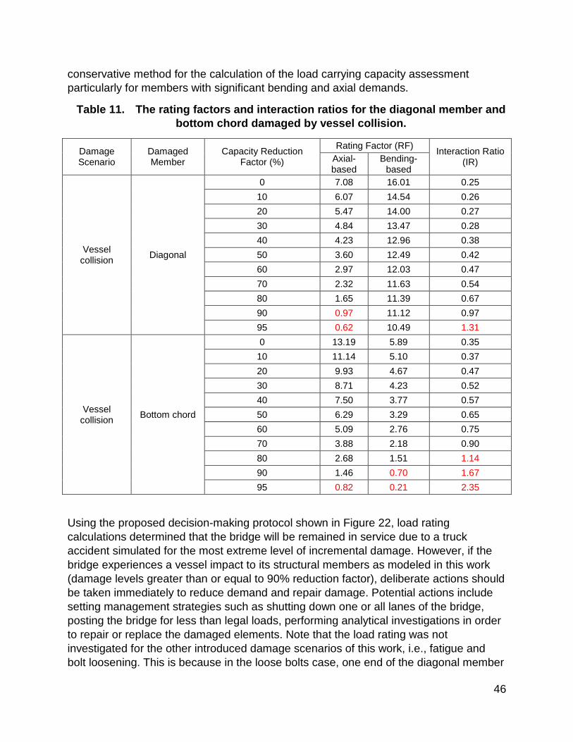
Figure 22. Flowchart for decision making based on load carrying capacity of the damaged bridge. .................................................................................................... 47
Figure 23. The acceleration time-history response during the lift action of the Memorial Bridge. 48
Figure 24. The acceleration time-history response during the lift action of the Memorial Bridge. Error! Bookmark not defined.
Figure 25. Simulating the lift action on the global model of the bridge using the dynamic moving load along the tower. ................................................................... 51
Figure 26. Numerical vs field collected strain response during upward lift action. ...... 52
Figure 27. Simulating three damage scenarios to the tower of the Memorial Bridge using the global FE model in LUSAS. .................................................................... 53
Figure 28. Time history strain responses of the strain rosettes at east side of the tower during lift action for healthy and damaged conditions. ........................................... 55
Figure 29. S-N curve of Fatigue categories by AASHTO [AASHTO, 2012]. ............... 57
Figure 30. Linear extrapolation to determine the hotspot stress at the weld toe (Niemi et al., 2016). ........................................................................................................... 59
Figure 31. The trend of the normalized fatigue responses with the increase in the days of data collection for different periods. ................................................................... 60
Figure 32. The monthly averaged fatigue responses for a one-year period of data collection. ............................................................................................................... 61
Figure 33. The six selected paths to determine the hot-spot and nominal stresses along the curved weld toe. ..................................................................................... 62
Figure 34. Variation of the numerical principal strain response with the distance to the weld toe for the six selected paths under the static truck load at (a) northbound (b) southbound. ........................................................................................................... 63
Figure 35. The SCF responses under the static truck load at the northbound and southbound. ........................................................................................................... 64
Figure 36. The assumed traffic scenario for simulation. ............................................. 65
Figure 37. The numerical (a) hotspot and (b) nominal time-history strain response for the selected paths under the dynamic traffic scenario in LUSAS. .......................... 66
Figure 38. Fatigue remaining life in the 75-year service life of the bridge, (a) hot spot stress, (b) nominal stress. ...................................................................................... 67
Figure 39. New Hampshire Residents view of Infrastructure Condition collected via the Granite State Pool Data collected in 2016 and 2017 .............................................. 75
10
Figure 40. Correlation between Survey Data on Infrastructure Condition and Pavement Condition Information ............................................................................ 76
Figure 41. Attachment of the tidal turbine to the Memorial Bridge, NH. ...................... 81
Figure 42. Tidal turbine support structure design. ...................................................... 83
Figure 43. Three-Dimensional Image (left) and SAP2000® Model (right) of the ......... 83
Figure 44. Applied live load to the A Frames. ............................................................. 85
Figure 45. Applied wind load to the platform. .............................................................. 86
Figure 46. Applied Drag load to the platform. ............................................................. 86
Figure 47. Applied drag load to the guideposts. ......................................................... 87
Figure 48. Applied the parallel wave load to the model. ............................................. 87
Figure 49. Applied perpendicular wave load to the model. ......................................... 87
Figure 50. Number label on the frame members. ....................................................... 89
Figure 51. Moment distribution in members under LC2 load combination. ................. 90
Figure 52. Anchor plate with four-anchor pattern. ....................................................... 92
Figure 53. Four-plate pattern (connection for one guide post). ................................... 93
Figure 54. Chain mooring system. .............................................................................. 95
Figure 55. Pile guide mooring system. ........................................................................ 95
Figure 56. Preparation of the VGPs on the fabrication company. ............................... 96
Figure 57. Coating and installation of the VGPs. ........................................................ 96
Figure 58. Instrumentation plan for vertical guide posts. ............................................ 97
Figure 59. Strain results at vertical guide posts for one day (12/19/2017). ................. 98
Figure 60. As-built plan for the vertical guide posts. ................................................... 98
Figure 61. The tidal turbine configuration. .................................................................. 99
Figure 62. Gt-Strudl® model of the tidal turbine deployment system. ........................ 100

11
Executive Summary This project included the “Living Bridge” group efforts to create a benchmark example of a self-diagnosing, self-reporting, “smart infrastructure” at the Memorial Bridge, NH-ME, to further advance a National Science Foundation (NSF) funded project, the “Living Bridge Project (LBP)”, seeking to promote infrastructure sustainability on three fronts by: (1) installing a small structural, environmental sensing network that is (2) powered by clean energy innovation in tidal energy conversion, while assessing how the tidal turbine installed at the bridge pier impacts the bridge structure and environment; and (3) deploying an innovative, interactive community engagement strategy. The structural design of the Memorial Bridge included several innovations (e.g., gusset-less truss connections) that were monitored and evaluated long-term through instrumentation and assessed for possible use on future infrastructure projects.
The proposed smart service system was mainly designed to take advantage of sensor technology and renewable energy conversion by installing a comprehensive structural, traffic and environmental sensing system to assess as accurately as possible bridge conditions in multiple key areas (e.g., traffic, structural integrity, environmental impact), and demonstrate the use of available tidal energy at estuarine bridges.
The project fulfilled the FHWA TIDP/AID program goals of Improving highway/bridge safety, reliability and service life, accelerating the adoption of innovative technologies, and improving highway/bridge sustainability and environmental protection.
The NHDOT was an eligible entity according to the AID Demonstration guidelines and Notice of Funding Availability. The proposed project was eligible for assistance under Title 23, United States Code, and initiated in 2016. The NHDOT accepted FHWA oversight of the project and worked with the FHWA to develop appropriate customer satisfaction measures.

12
Introduction The Memorial Bridge, constructed in 2013, is a “gusset-less” steel truss vertical lift bridge spanning Piscataqua River between Portsmouth, NH, and Kittery, ME, carrying traffic of US Route 1. This bridge is the only pedestrian link between Portsmouth and Kittery and serves an important infrastructure function by connecting the two communities via walking and biking. The “Living Bridge” team, which includes the owner (NHDOT/MEDOT), bridge designer (HNTB), contractor (Archer/Western), and University of New Hampshire (UNH), has developed plans to enhance the bridge monitoring system to advance bridge design, construction, maintenance, and traffic management.
Accelerated Innovation Deployment (AID) Demonstration Grants
The Federal Highway Administration (FHWA) AID Demonstration Grants Program, which is administered through the FHWA Center for Accelerating Innovation (CAI), provides incentive funding and other resources for eligible entities to offset the risk of trying an innovation and to accelerate the implementation and adoption of that innovation in highway transportation. Entities eligible to apply include State departments of transportation (DOTs), Federal land management agencies, and tribal governments as well as metropolitan planning organizations and local governments which apply through the State DOT as subrecipients.
The AID Demonstration program is one aspect of the multi-faceted Technology and Innovation Deployment Program (TIDP). AID Demonstration funds are available for any project eligible for assistance under title 23, United States Code. Projects eligible for funding shall include proven innovative practices or technologies such as those included in the Every Day Counts (EDC) initiative. Innovations may include infrastructure and non-infrastructure strategies or activities, which the award recipient intends to implement and adopt as a significant improvement from their conventional practice.
Report Scope and Organization
This report documents the New Hampshire Department of Transportation demonstration grant award for creation of a sustainable transportation infrastructure using innovative techniques and methodologies to advance the state of the art for bridge condition assessment, traffic management, and structural health and environmental stewardship, in addition to serving as a community platform to educate the general public about how incorporating renewable energy into bridge design can lead to a sustainable transportation infrastructure with impact far beyond the region. This report presents information related to the employed project innovation(s), the overarching TIDP goals, performance metrics measurement and analysis, lessons learned, and the status of activities related to adoption of smart sensing systems and clean energy conversion as conventional practice by the New Hampshire Department of Transportation.

13
The appendix of this report include the design development, calculations and structural performance prediction of the vertical guide posts that connect the tidal turbine deployment platform to Pier 2 at the Memorial Bridge, connecting Portsmouth, NH and Kittery, ME.
Project Overview The Living Bridge: The Future of Smart, Sustainable, User-Centered Transportation Infrastructure, was enabled through partnerships between academic researchers with expertise in structural, mechanical and ocean engineering, sensing technology and social science, as well as business partners with expertise in bridge design, instrumentation, data collection, and tidal energy conversion. The Memorial Bridge has been instrumented with sensors that can proactively monitor structural performance, traffic patterns, operational and environmental variations, and the behavior of innovative bridge design elements (e.g., gusset-less truss connections), and enable one to promote community engagement.
As described in Table 1, AID Demonstration funding was used to finance the deployment of sensor network for structural health and environment monitoring, assessment of structural performance, and development of guidelines to create smart bridges that incorporate monitoring systems and structural modeling into their design, construction and maintenance, and enhance traffic management programs.
Table 1. Table Project objectives and relationship to TIDP/AID program goals.
Project Objectives
1 Deploying sensor network at the “Living Bridge” for structural health and environment monitoring X X
2 Monitoring/assessing infrastructure performance (structural integrity and the impact of traffic and lift span operation) X X X
3 Developing guidelines to create smart bridges that incorporate monitoring systems and structural modeling into their design, construction and maintenance and enhance traffic management programs
X X
TIDP and AID Goals (Selected) A B C A Improve highway/bridge safety, reliability and service life B Improve highway/bridge sustainability and environmental protection
C Significantly accelerate the adoption of innovative technologies by the surface transportation community.
14
Project Details
Background
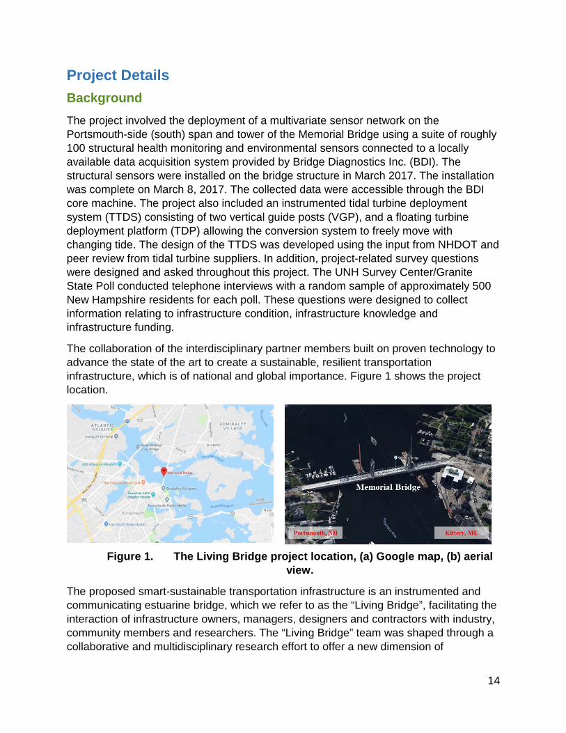
The project involved the deployment of a multivariate sensor network on the Portsmouth-side (south) span and tower of the Memorial Bridge using a suite of roughly 100 structural health monitoring and environmental sensors connected to a locally available data acquisition system provided by Bridge Diagnostics Inc. (BDI). The structural sensors were installed on the bridge structure in March 2017. The installation was complete on March 8, 2017. The collected data were accessible through the BDI core machine. The project also included an instrumented tidal turbine deployment system (TTDS) consisting of two vertical guide posts (VGP), and a floating turbine deployment platform (TDP) allowing the conversion system to freely move with changing tide. The design of the TTDS was developed using the input from NHDOT and peer review from tidal turbine suppliers. In addition, project-related survey questions were designed and asked throughout this project. The UNH Survey Center/Granite State Poll conducted telephone interviews with a random sample of approximately 500 New Hampshire residents for each poll. These questions were designed to collect information relating to infrastructure condition, infrastructure knowledge and infrastructure funding.
The collaboration of the interdisciplinary partner members built on proven technology to advance the state of the art to create a sustainable, resilient transportation infrastructure, which is of national and global importance. Figure 1 shows the project location.
Figure 1. The Living Bridge project location, (a) Google map, (b) aerial
view.
The proposed smart-sustainable transportation infrastructure is an instrumented and communicating estuarine bridge, which we refer to as the “Living Bridge”, facilitating the interaction of infrastructure owners, managers, designers and contractors with industry, community members and researchers. The “Living Bridge” team was shaped through a collaborative and multidisciplinary research effort to offer a new dimension of

15
sustainability and management to the traditional bridge design protocol. Each of the technologies proposed here were designed and tested individually for a variety of purposes. Technical areas involved structural health and estuarine monitoring, tidal energy conversion, and community engagement (see Figure 2).
Figure 2. Technical areas of the Living Bridge project.
Current institutional experience
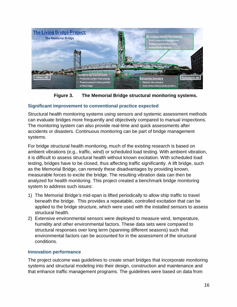
At the time of submitting the project proposal, the NHDOT was managing two bridges with active structural monitoring programs as well as a traffic management monitoring program dispersed throughout the state. This project was the first case where structural, traffic, and environmental monitoring programs were integrated. The proposed project has been conducted in partnership with the UNH faculty members who have significant experience in the area of structural health monitoring and structural parameter estimation. Figure 3 highlights the project innovations and the structural health/estuary monitoring systems on the Memorial Bridge (west face).
16
Figure 3. The Memorial Bridge structural monitoring systems.
Significant improvement to conventional practice expected
Structural health monitoring systems using sensors and systemic assessment methods can evaluate bridges more frequently and objectively compared to manual inspections. The monitoring system can also provide real-time and quick assessments after accidents or disasters. Continuous monitoring can be part of bridge management systems.
For bridge structural health monitoring, much of the existing research is based on ambient vibrations (e.g., traffic, wind) or scheduled load testing. With ambient vibration, it is difficult to assess structural health without known excitation. With scheduled load testing, bridges have to be closed, thus affecting traffic significantly. A lift bridge, such as the Memorial Bridge, can remedy these disadvantages by providing known, measurable forces to excite the bridge. The resulting vibration data can then be analyzed for health monitoring. This project created a benchmark bridge monitoring system to address such issues:
1) The Memorial Bridge’s mid-span is lifted periodically to allow ship traffic to travel beneath the bridge. This provides a repeatable, controlled excitation that can be applied to the bridge structure, which were used with the installed sensors to assess structural health.
2) Extensive environmental sensors were deployed to measure wind, temperature, humidity and other environmental factors. These data sets were compared to structural responses over long term (spanning different seasons) such that environmental factors can be accounted for in the assessment of the structural conditions.
Innovation performance
The project outcome was guidelines to create smart bridges that incorporate monitoring systems and structural modeling into their design, construction and maintenance and that enhance traffic management programs. The guidelines were based on data from

17
the “Living Bridge” on structural integrity assessment, and bridge maintenance protocols using SHM, traffic management and environmental impact. It was demonstrated that the sensors and technologies proposed for the “Living Bridge” can become common for future “smart” bridges, and result in significant cost savings during the life-span of the bridge, as explained in Table 2.
Table 2. Assessment of innovation performance.
Monitoring System
• Compare structural measures/assessments with bridge inspections • Use traffic sensors to refine the intelligent transportation management
system in NH • Use environmental sensors for extreme event traffic management in
coastal regions • Calibrate a structural model for bridge management
Public outreach
The major innovation of this partnership was the integration of the proposed technologies to create a smart, self-reporting, and self-diagnosing bridge that can permanently monitor everything from structural stability to traffic and environmental variabilities, in addition to educating the public and explorers of all ages about the impact and effectiveness of emerging technologies on bridge sustainability and environmental protection (see Figure 4).
Figure 4. Public outreach on bridge sustainability and environmental
protection.
Applicant information and coordination with other entities
The project applicant is the New Hampshire Department of Transportation (NHDOT). The project was conducted in partnership with the University of New Hampshire and the FHWA – NH Division. This proposal was the culmination of an effort over the past years in which NHDOT, the community, university faculty and students, and the commercial sector have participated to develop the “Living Bridge” project. The NHDOT participated in monitoring and assessment activities regarding the effectiveness of the innovation, provided information for technology transfer including specifications and lessons

18
learned, and delivered a written report summarizing the above within 6 months of completion of the project.

19
Project Description
The focus of this report is the efforts made with respect to the structural health monitoring component of the Living Bridge project, as the funding supported by the FHWA TIDP/AID program was used to leverage the structural monitoring infrastructure created by the NSF funded project. The “Living Bridge” team, led by NHDOT, installed a variety of structural health monitoring sensors (described in Table 3) on key structural elements and the tidal turbine deployment system of the Memorial Bridge.
The sensor data is not only valuable to capture the response of critical bridge elements to truck traffic but also the response due to the vertical lift operations and the environmental variations due to the coastal location. This section will detail the data collection protocols, the structural model creation and validation, global modeling updating and load rating, local model damage detection and fatigue assessment. The last part of this section will present the vertical guide post that support the tidal turbine deployment system.
Table 3. Structural health monitoring sensors.
Type of SHM Sensors Number of Sensors Total Number of Sensor
Channels East Face West Face Uniaxial Accelerometer (1 channel) 9 3 12
Rosette Strain Gage (3 channels) 14 2 48
Uniaxial Strain Gage (1 channel) 5 5 10
Biaxial Tiltmeter (2 channels) 2 0 4
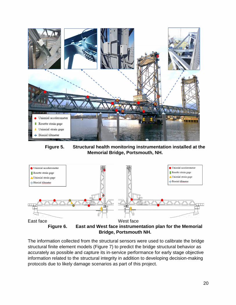
The structural sensors and the current instrumentation layout are shown in Figure 5 and Figure 6.
20
Figure 5. Structural health monitoring instrumentation installed at the Memorial Bridge, Portsmouth, NH.
East face West face
Figure 6. East and West face instrumentation plan for the Memorial Bridge, Portsmouth NH.
The information collected from the structural sensors were used to calibrate the bridge structural finite element models (Figure 7) to predict the bridge structural behavior as accurately as possible and capture its in-service performance for early stage objective information related to the structural integrity in addition to developing decision-making protocols due to likely damage scenarios as part of this project.

21
Figure 7. The calibrated structural models of the bridge using the
resulting structural response obtained through a pseudo-static (truck) load testing; left: SAP2000® model, right: Lusas® model.
The results from the SAP2000® model were also used to predict the demands the Memorial Bridge will experience in both its lifted and un-lifted positions in variable environmental conditions due to wind loads such that the viability of a lift can be more objectively defined. These results were compiled in conjunction with bridge’s aerodynamic susceptibility and an investigation of the dynamics of the bridge’s counterweight system, both of which were found to be of minimal concern in terms of bridge structural safety. Following the future integration of structural health monitoring (SHM) and weather data acquisition systems at the case study site, the proposed protocol will be refined and expanded to more accurately predict safe lifting conditions [Nash, 2016 and Nash et al., 2018].
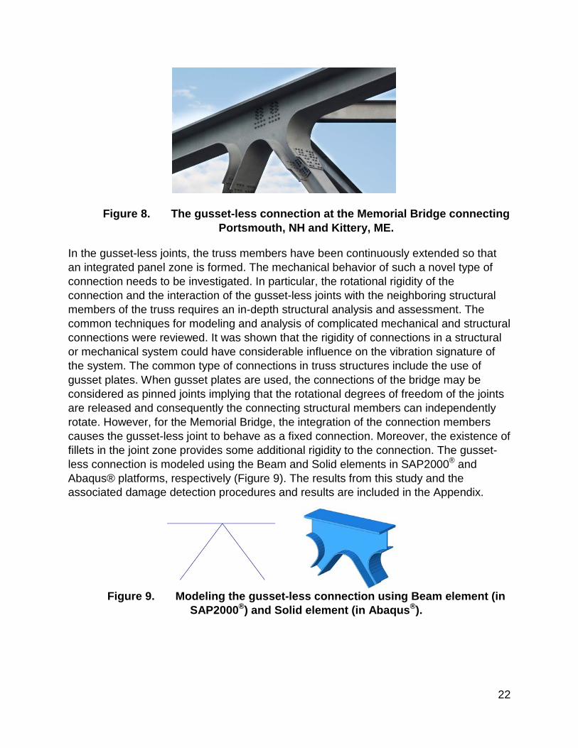
One of the innovative structural features of the new Memorial Bridge is removing gusset plates in the connection zones of the bridge truss. To verify design assumptions and characterize the fatigue behavior of the bridge main structural innovation (i.e., the “gusset-less” truss connections shown in Figure 8). The field-collected performance data, laboratory experimental testing, and physics-based structural modeling were integrated to develop a protocol to assess the condition and predict the remaining life of the gusset-less truss connections used at the Memorial Bridge. It is anticipated that the aforementioned approach will be modified to develop a framework to extend this protocol for application to future innovative structural elements.
22
Figure 8. The gusset-less connection at the Memorial Bridge connecting Portsmouth, NH and Kittery, ME.
In the gusset-less joints, the truss members have been continuously extended so that an integrated panel zone is formed. The mechanical behavior of such a novel type of connection needs to be investigated. In particular, the rotational rigidity of the connection and the interaction of the gusset-less joints with the neighboring structural members of the truss requires an in-depth structural analysis and assessment. The common techniques for modeling and analysis of complicated mechanical and structural connections were reviewed. It was shown that the rigidity of connections in a structural or mechanical system could have considerable influence on the vibration signature of the system. The common type of connections in truss structures include the use of gusset plates. When gusset plates are used, the connections of the bridge may be considered as pinned joints implying that the rotational degrees of freedom of the joints are released and consequently the connecting structural members can independently rotate. However, for the Memorial Bridge, the integration of the connection members causes the gusset-less joint to behave as a fixed connection. Moreover, the existence of fillets in the joint zone provides some additional rigidity to the connection. The gusset-less connection is modeled using the Beam and Solid elements in SAP2000® and Abaqus® platforms, respectively (Figure 9). The results from this study and the associated damage detection procedures and results are included in the Appendix.
Figure 9. Modeling the gusset-less connection using Beam element (in
SAP2000®) and Solid element (in Abaqus®).

23
Data Collection and Analysis
Performance measures consistent with the project goals were jointly established for this project by NHDOT and FHWA to qualify, not to quantify, the effectiveness of the innovation to inform the AID Demonstration program in working toward best practices, programmatic performance measures, and future decision-making guidelines.
Data was collected to determine the impact of using structural and environmental monitoring data on bridge safety and serviceability, traffic/bridge management, and intelligent transportation management systems in NH and demonstrate the ability to:
• Achieve a safer environment for the traveling public and workers. SHM: Real-time monitoring of the bridge structural performance
o A bridge outfitted with a network of multiple real-time sensors at sparse locations throughout the structure able to effectively monitor the structural performance under operating conditions and make aware the bridge managers of any abnormal change in the actual condition of the structure. Advanced SHM methods using sensors, data collection, and analysis could greatly improve the ability of engineers to contribute to overall public safety.
• Reduce overall project delivery time and associated costs. SHM: Not initially considered on the SHM program of this project.
o The proposed structural health monitoring system was not initially considered to reduce overall project delivery time and associated costs in this project.
• Reduce life cycle costs through producing a high-quality project. SHM: Setting-up alarm systems to advise bridge owners on maintenance strategies required to reduce life cycle costs associated with bridge maintenance and management.
o Structural health monitoring systems could help establish automated and early warning systems that are able to alert maintenance engineers when there is a slight change in system response or when a pre-defined damage reaches a length that require repair or replacement. In addition to helping bridge managers recognize poor structural components and better decide on maintenance strategies, new monitoring technologies could also help professionals determine potential future risks to safety and reduce the likelihood of catastrophic structural failures and damage.
• Reduce impacts to the traveling public and project abutters. SHM: Minimizing traffic delay due to maintenance needs.
o Traffic delay due to maintenance needs could be minimized as SHM systems do not need to stop traffic for initial instrumentation of the structure.
• Satisfy the needs and desires of our customers. SHM: Satisfy the needs for bridge future maintenance and management by NHDOT.

24
o The proposed SHM technology can have a number of benefits, from improving safety standards and reducing risks, to discovering new opportunities to reduce costs.
This section discusses how the NHDOT established baseline criteria, monitored and recorded data during the implementation of the innovation, and analyzed and assessed the results for each of the performance measures related to these focus areas.
Application of Field Collected SHM Data of the Memorial Bridge
Data collection program at the Memorial Bridge
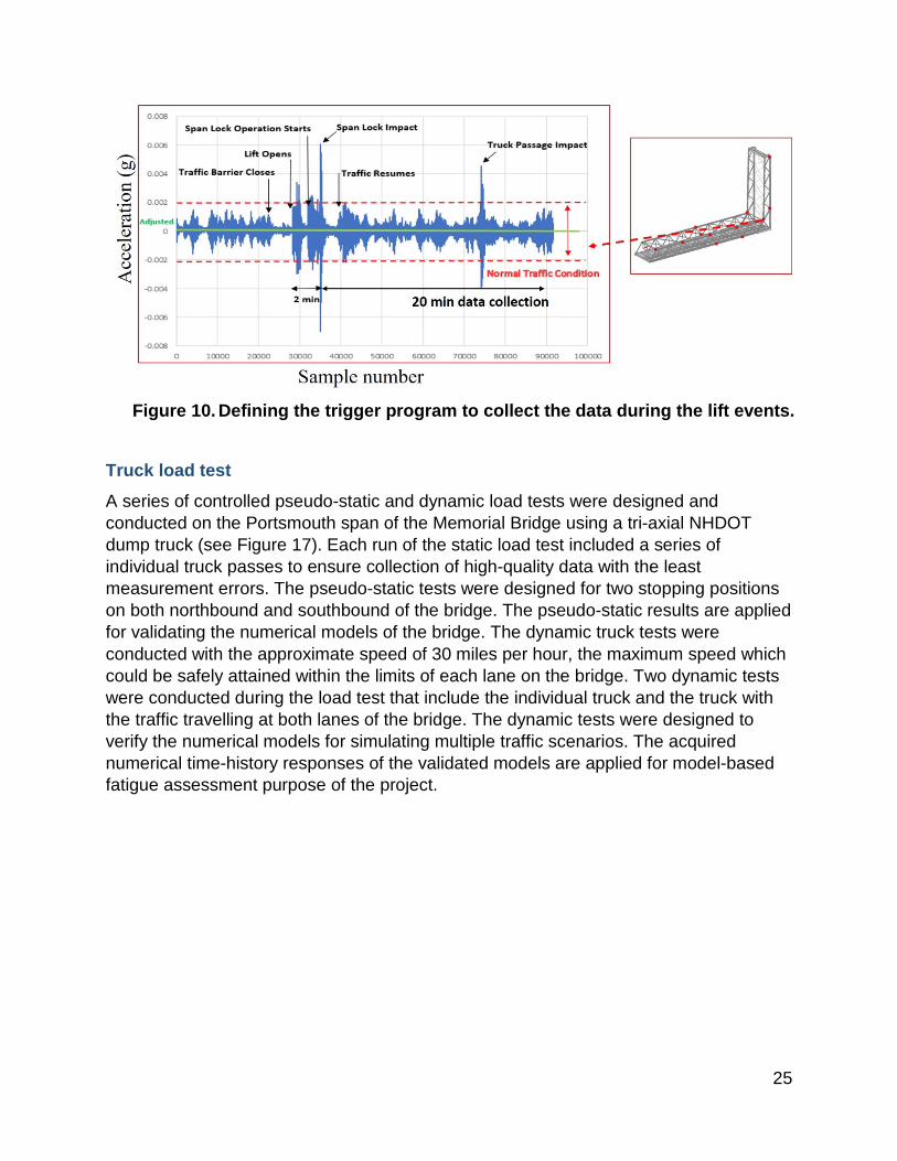
In the SHM program of the Memorial Bridge, three types of data are collected including decimated, normal, and event data shown in Table 4. The decimated data, and the high-speed normal data are collected continuously to study the daily trends and the detailed performance of the bridge respectively. The event data is collected via a triggered program which starts for data collection corresponding to the lift actions and continues for the 20-minutes period after each lift. This time interval was selected based on the initial observations of the monitoring data, which ensures to collect the data during a considerable traffic volume congested after each lift action. Consequently, the number of the samples collected per day can vary corresponding to the number of the lift actions experienced in each day. In addition, the duration of the lift and fall of the midspan is identical for all of the lift events. However, the duration of Midspan stay depends on the naval traffic. In Figure 10, the time-history acceleration responses of the accelerometer that is investigated to be the most sensitive data acquisition system to the lift excitations is shown. The acceleration threshold for the trigger program is defined based on the acceleration responses of this accelerometer. The 20-minues duration of after lift data collection is defined based on the traffic records by the video camera, installed at the bridge. However, it is observed that the lift events that occur at less traffic hours may not significantly include traffic-induced stress cycles.
Table 4. Data collection program at the Memorial Bridge.
Type of data Sample rate (Hz)
Daily data collection Objective
Decimated 600 Continuous (24 hour) The overall trend
Normal 50 Continuous (24 hour)
Condition Assessment
Event 50 Lift Event triggered
(20 Minutes)
Lift operation assessment
25
Figure 10. Defining the trigger program to collect the data during the lift events.
Truck load test
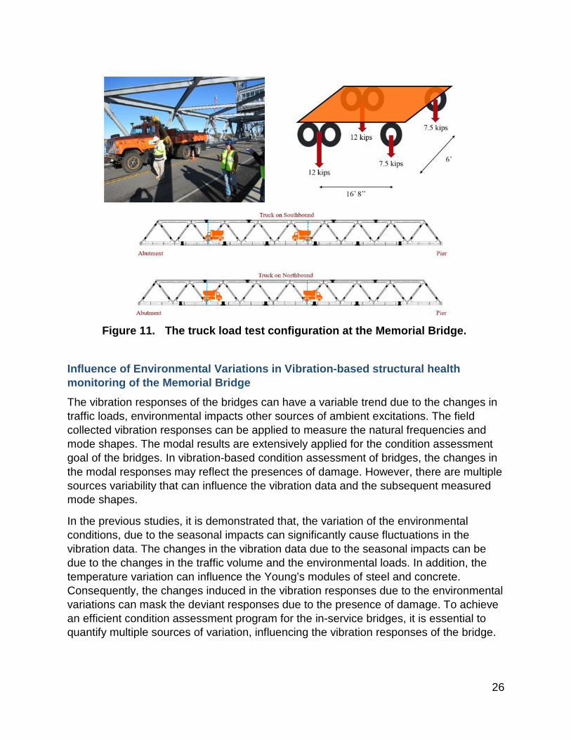
A series of controlled pseudo-static and dynamic load tests were designed and conducted on the Portsmouth span of the Memorial Bridge using a tri-axial NHDOT dump truck (see Figure 17). Each run of the static load test included a series of individual truck passes to ensure collection of high-quality data with the least measurement errors. The pseudo-static tests were designed for two stopping positions on both northbound and southbound of the bridge. The pseudo-static results are applied for validating the numerical models of the bridge. The dynamic truck tests were conducted with the approximate speed of 30 miles per hour, the maximum speed which could be safely attained within the limits of each lane on the bridge. Two dynamic tests were conducted during the load test that include the individual truck and the truck with the traffic travelling at both lanes of the bridge. The dynamic tests were designed to verify the numerical models for simulating multiple traffic scenarios. The acquired numerical time-history responses of the validated models are applied for model-based fatigue assessment purpose of the project.
26
Figure 11. The truck load test configuration at the Memorial Bridge.
Influence of Environmental Variations in Vibration-based structural health monitoring of the Memorial Bridge
The vibration responses of the bridges can have a variable trend due to the changes in traffic loads, environmental impacts other sources of ambient excitations. The field collected vibration responses can be applied to measure the natural frequencies and mode shapes. The modal results are extensively applied for the condition assessment goal of the bridges. In vibration-based condition assessment of bridges, the changes in the modal responses may reflect the presences of damage. However, there are multiple sources variability that can influence the vibration data and the subsequent measured mode shapes.
In the previous studies, it is demonstrated that, the variation of the environmental conditions, due to the seasonal impacts can significantly cause fluctuations in the vibration data. The changes in the vibration data due to the seasonal impacts can be due to the changes in the traffic volume and the environmental loads. In addition, the temperature variation can influence the Young’s modules of steel and concrete. Consequently, the changes induced in the vibration responses due to the environmental variations can mask the deviant responses due to the presence of damage. To achieve an efficient condition assessment program for the in-service bridges, it is essential to quantify multiple sources of variation, influencing the vibration responses of the bridge.

27
The long-term data collection program at the Memorial Bridge, provides the opportunity to investigate the influence of environmental variations (due to the seasonal impacts) on the trend of the collected vibration responses of the bridge. The vibration response of the Memorial Bridge is primarily induced by the traffic loads and the lift excitations. The changes in the traffic pattern and the frequency of the lift action are dependent on the seasonal variations. In addition, the lift action of the Memorial Bridge has an on-demand property, that influences the schedule and frequency of the daily reported lift actions. Consequently, the changes in the trend of vibration responses of the bridge can be significantly influenced by the seasonal variations of the lift program.
The long-term SHM program of the Memorial bridge includes an array accelerometer, that collect continuous vibration data from multiple locations, at the south span and south tower of the bridge. Depending on the location of the installed accelerometer, the collected vibration responses can be influenced by the traffic load and/or lift operation. The accelerometers, that are installed at the tower, can dominantly collect the vibration responses during the lift and drop action. Correspondingly, the accelerometers, that are installed at the south span of the bridge, can significantly report the traffic-induced vibrations. In addition, depending on the location of the accelerometer, the influence of various environmental conditions on the collected vibration responses can be different.
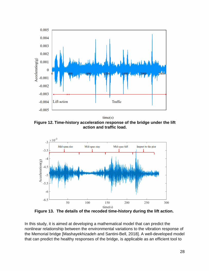
In Figure 12, the time history acceleration response of the bridge during the lift action and the traffic load is shown. The location of data collection is also displayed. As shown in Figure 13, the lift action consists of the lift, drop and the impact parts. The impact part of the vibration responses happens when the mid-span hits the bridges’ pier. A high amplitude excitation is generated at the multiple location of the bridge, as compared to the upward and downward responses. The traffic- induced vibration has a more variable response as compared to the lift-induced vibration responses.
28
Figure 12. Time-history acceleration response of the bridge under the lift
action and traffic load.
Figure 13. The details of the recoded time-history during the lift action.
In this study, it is aimed at developing a mathematical model that can predict the nonlinear relationship between the environmental variations to the vibration response of the Memorial bridge [Mashayekhizadeh and Santini-Bell, 2018]. A well-developed model that can predict the healthy responses of the bridge, is applicable as an efficient tool to

29
detect the deviated responses due to a possible damage. To study the influence of the environmental-induced variations on the vibration responses of the Memorial Bridge, the vibration data are collected from multiple locations of the bridge. Three different accelerometers, that are installed at distinctive locations of the bridge, are selected for the study. The selection of the accelerometers is made based on the sensitivity of the data acquisition system to capture the excitations, induced by the traffic load and lift actions.
The locations of the selected accelerometers are shown in Figure 14. A-3, located at the top chord of the south span, can significantly report the traffic induced vibration and is less sensitive to the lift-induced vibrations. A-10, installed at the top of the tower, is selected to report the vibration responses during the lift operation system. The A-10 accelerometer that is located at the top of the tower, is highly influenced by the upward and downward movement of the lift span. A-8 is located at the bottom of the tower, where the tower is connected to the south span. A-8 accelerometer can capture the vibrations responses due to the traffic loads as well as the lift action. In addition, this accelerometer is closer the pier of the bridge and can receive the excitations that are induced by the impact of the midspan to the pier of the bridge. In Table 5, through the selected accelerometers, the variability of the vibration responses due to the environmental condition can be discriminated to the traffic load and lift action.
Figure 14. Selected accelerometers for vibration data collection.
Table 5. The location and type of data collected at the selected accelerometers.
Accelerometer # Collected data Location A-3 Traffic-induced vibration Top chord/ top flange A-8 Traffic & Lift vibration Tower/south flange A-10 Lift induced vibration Tower/ south flange

30
Environmental data collection
To investigate the environmental variations of the field, multiple environmental information, including wind, temperature and humidity are collected, for this study. The environmental data are collected through the weather station, that is installed at the top of the south tower of the bridge. The weather station can collect ambient environmental information. However, the recorded ambient temperature at the weather station can be different to the surface experienced temperature, at multiple locations of the bridge. The influence of solar radiation can also cause changes the surface temperature at multiple locations of the bridge. In addition, the difference between the experienced temperature at the location of the accelerometer to the recorded ambient temperature can influence the accuracy of the results.
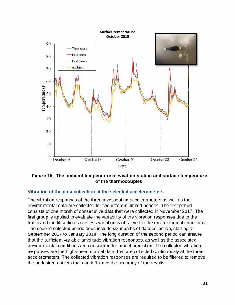
To investigate the differences between the surface and ambient temperature, for a limited period, multiple thermocouples were installed at the east and west side of the south span and the tower of the bridge. The time-history responses of the ambient temperature are compared to the collected surface-temperature responses, as shown in Figure 15. A similar trend is observed between the recorded surface temperatures and the ambient temperature. However, the thermocouple, that is temporarily installed at the east side of the tower, as compared to the other thermocouples, reported the higher amplitude responses in the picks of the time-history response. The recorded ambient temperature responses can be exclusively calibrated with the surface temperature data for the three investigating accelerometers. The calibrated temperature data are applied as the classifying features to be applied for predicting the vibration response of the bridge.
31
Figure 15. The ambient temperature of weather station and surface temperature of the thermocouples.
Vibration of the data collection at the selected accelerometers
The vibration responses of the three investigating accelerometers as well as the environmental data are collected for two different limited periods. The first period consists of one month of consecutive data that were collected in November 2017. The first group is applied to evaluate the variability of the vibration responses due to the traffic and the lift action since less variation is observed in the environmental conditions. The second selected period does include six months of data collection, starting at September 2017 to January 2018. The long duration of the second period can ensure that the sufficient variable amplitude vibration responses, as well as the associated environmental conditions are considered for model prediction. The collected vibration responses are the high-speed normal data, that are collected continuously at the three accelerometers. The collected vibration responses are required to be filtered to remove the undesired outliers that can influence the accuracy of the results.
32
Processing the data including the vibration and the environmental time-history data
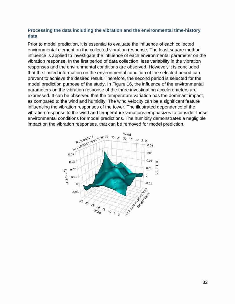
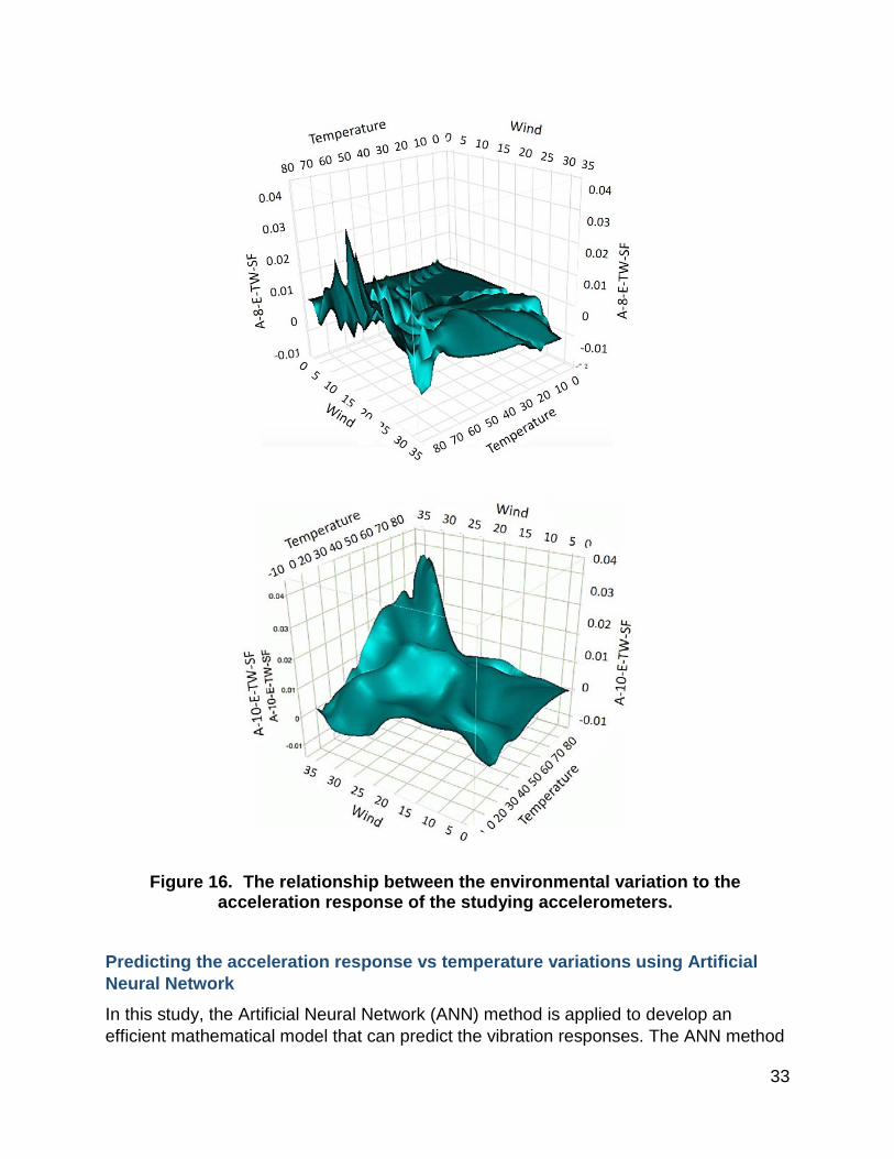
Prior to model prediction, it is essential to evaluate the influence of each collected environmental element on the collected vibration response. The least square method influence is applied to investigate the influence of each environmental parameter on the vibration response. In the first period of data collection, less variability in the vibration responses and the environmental conditions are observed. However, it is concluded that the limited information on the environmental condition of the selected period can prevent to achieve the desired result. Therefore, the second period is selected for the model prediction purpose of the study. In Figure 16, the influence of the environmental parameters on the vibration response of the three investigating accelerometers are expressed. It can be observed that the temperature variation has the dominant impact, as compared to the wind and humidity. The wind velocity can be a significant feature influencing the vibration responses of the tower. The illustrated dependence of the vibration response to the wind and temperature variations emphasizes to consider these environmental conditions for model predictions. The humidity demonstrates a negligible impact on the vibration responses, that can be removed for model prediction.
33
Figure 16. The relationship between the environmental variation to the acceleration response of the studying accelerometers.
Predicting the acceleration response vs temperature variations using Artificial Neural Network
In this study, the Artificial Neural Network (ANN) method is applied to develop an efficient mathematical model that can predict the vibration responses. The ANN method
34
is extensively applied in predicting the pattern of the variable amplitude SHM responses. The accurate prediction of an ANN model depends on the accuracy as well as sufficiency of the collected information, that can describe the variation of the objective response. In this study, the environmental information, the month and the season of data collection are also considered as the influential parameters for model prediction. The collected data are trained to predict the relationship between the influential features to the vibration response.
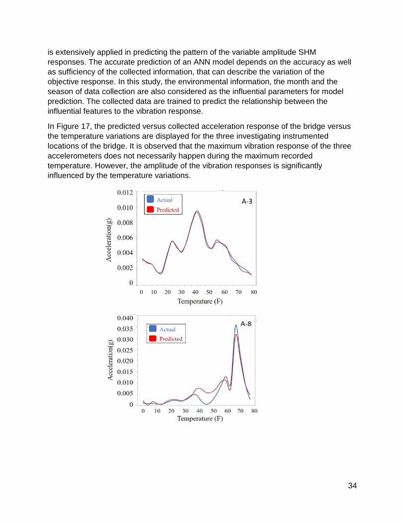
In Figure 17, the predicted versus collected acceleration response of the bridge versus the temperature variations are displayed for the three investigating instrumented locations of the bridge. It is observed that the maximum vibration response of the three accelerometers does not necessarily happen during the maximum recorded temperature. However, the amplitude of the vibration responses is significantly influenced by the temperature variations.

35
Figure 17. Actual vs predicted acceleration responses with temperature
variation at A-3, A-8, A-10 accelerometers.
In addition, an acceptable agreement is observed between the collected and predicted vibration responses of the three-investigating accelerometers. A-3 accelerometer, reporting the traffic data, has a more compatible predicted responses compared to the collected vibration responses. The efficiency in predicting the traffic induced vibration responses indicates that the changes in the traffic load and the induced vibration responses is highly dependent on the environmental variations. However, the vibration response due to the lift action can be more predictable as compared to the traffic excitations. The predicted responses at A-10 can slightly be different in the picks of the vibration response.
Accelerometer A-8, collecting the vibration responses due to the traffic and the lift action, shows a less predictable response, as compared to the two other accelerometers. As shown in Figure 4 (c), in some parts of the graph the predicted responses are not compatible to the collected vibration responses at the location. The A-8 collects the excitations due to the traffic load, the upward and downward movement of the mid-span and the impact loads due to the midspan to the pier of the bridge. However, the vibration responses due to the impact action are more influenced by the damping system as well as the mechanical system of the lift. Therefore, more information, apart from the environmental data, are required to be collected to achieve a more desirable predicted response.
In the three investigating locations, it is illustrated that the temperature variation has a significant impact on the variability of the vibration response. To create a comprehensive model that can predict the nonlinear relationship of the temperature to the vibration responses at multiple locations of the bridges, a wider range of temperature and wind variations can be beneficial. The required range of environmental data for model prediction is significantly dependent on the climate conditions at the area

36
of study. In Portsmouth, NH, less frequent lift action and traffic volume is recorded in the below freezing period. However, it is recommended to consider the vibration response as well as the environmental data of the below freezing days, in developing an efficient ANN model [Mashayekhizadeh, Santini-Bell, 2018a]. The result of this study is presented in 27th ASNT research symposium, 2018, Orlando, Fl. and the ICNET 2018, Portsmouth, NH.

37
The Structural Model Creation and Validation
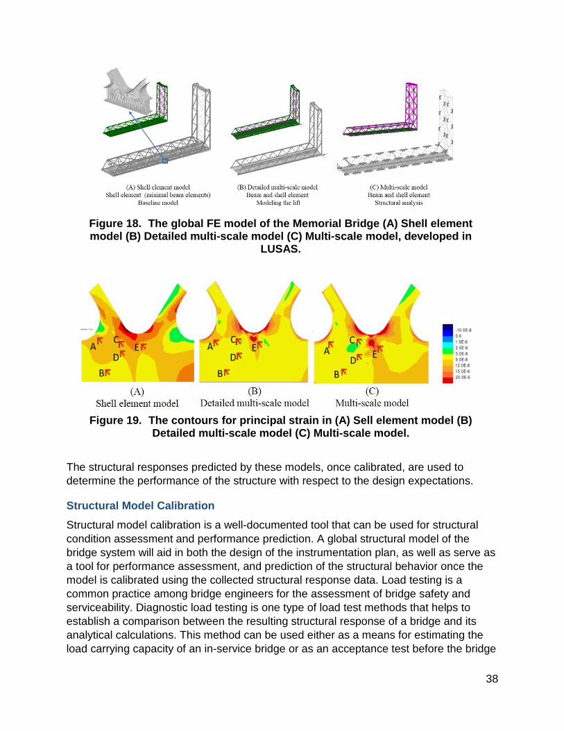
The complexity of the structural elements particularly the gusset-less connections of the Memorial Bridge necessitates a detailed Finite Element (FE) model; hence, a set of detailed FE models were simultaneously created in Lusas® to assess the data given the complexity to the gusset-less connection, see Figure 18. In this study, three different global FE models are developed, meeting specific goal of the project. The models differ in the number and type of the element. A beam-element structural model was also created in SAP2000® for limited use for global model updating and damage detection and resulting load rating. This model will be discussed in the “Global Structural Condition Assessment” section.
The first model is the shell element model that all the structural members are modeled with shell elements. The shell elements are the three-dimensional 4-noded thick shell element having 6-nodal degrees of freedom (DOF). This model is developed to study the continuous stress variations between the gusset-less connection and the other connecting members to the connection. In addition, the model is considered as a basic model in developing the efficient multi-scale models. The second model is the multi-scale model that considers the beam elements and shell elements in the model. The east and west truss of the bridge, as well as the deck of the bridge are modeled with shell element. The long members that are in the out-of-plane direction of the trusses are modeled with beam element. These long members include the braces in the tower and the top of the south span, the floor beams and the skewed floor beams. The selection of these members is based on the beam-like performance of the members, observed in the Shell element model. The reduction in the dimension of the selected members can significantly increase the efficiency of the model by reducing the computation time. The beam elements are the three-dimensional thick beam elements that have 6-nodal DOFs. This model is developed for simulating the lifting action of the bridge.
The third model is the multi-scale model that the gusset-less connections and the deck of the bridge are modeled with beam elements. The reminder long members are modeled with the beam elements. Similar beam and shell elements are applied in this model. The coupling of the shell to the beam elements are performed using multi-point constraint equation method [Mashayekhi & Santini-Bell, 2018]. This model is developed for an efficient performance assessment of the gusset-less connections under the traffic loads, which is applied for fatigue assessment of the connection. The strain contours of the three models at the gusset-less connection under the static truck load test (second stop) are compared in Figure 19. It can be observed that the multi-scale models can appropriately show similar structural responses as compared to the single scale shell element model.
38
Figure 18. The global FE model of the Memorial Bridge (A) Shell element model (B) Detailed multi-scale model (C) Multi-scale model, developed in
LUSAS.
Figure 19. The contours for principal strain in (A) Sell element model (B) Detailed multi-scale model (C) Multi-scale model.
The structural responses predicted by these models, once calibrated, are used to determine the performance of the structure with respect to the design expectations.
Structural Model Calibration
Structural model calibration is a well-documented tool that can be used for structural condition assessment and performance prediction. A global structural model of the bridge system will aid in both the design of the instrumentation plan, as well as serve as a tool for performance assessment, and prediction of the structural behavior once the model is calibrated using the collected structural response data. Load testing is a common practice among bridge engineers for the assessment of bridge safety and serviceability. Diagnostic load testing is one type of load test methods that helps to establish a comparison between the resulting structural response of a bridge and its analytical calculations. This method can be used either as a means for estimating the load carrying capacity of an in-service bridge or as an acceptance test before the bridge

39
is put into service. Given a controlled load test, the calibrated models would be beneficial to be used for operational decisions such as those relating to maintenance scheduling and overweight vehicle permitting.
Creating a calibrated structural model that can predict the impact of operational and environmental variations on the lift operation and bridge performance will allow for the creation of a data-driven decision-making matrix for fatigue performance prediction, load rating deterioration and real-time condition assessment.
Table 6 shows the comparison of the natural frequencies of the bridge obtained through the monitoring data and those predicted by the analytical models (SAP2000® and Lusas®) of the bridge.
Table 6. The comparison of the bridge natural frequencies with their counterparts obtained from the analytical models.
Natural frequencies (Hz) Mode number SAP2000® LUSAS® Monitoring Data
1 1.23 1.212 1.61 2 2.04 2.05 2.51 3 4.17 4.04 4.77
The strain responses acquired through the structural analysis of the developed FE models are compared to the field data in Table 7. The structural response data in Table 7 illustrates that the detailed multi-scale model produces lower strain responses indicating as stiffer connection, as expected with more beam elements, when compared to the multi-scale and shell element models. Consequently, it was found that the detailed multi-scale model shows a better agreement to the field data compared to other models.
Table 7. The comparison between the numerical strain responses of the FE models and field strain responses.
Strain gauge (location)
Shell element model
(¼µ)
Detailed Multi-scale model
(¼µ)
Multi-scale model
(¼µ)
Field data (¼µ)
A 8.03 7.99 7.86 7.50 B 6.22 6.15 7.79 8.21
C 7.98 7.85 7.93 8.00
D 7.66 6.40 6.52 7.62
E 10.82 10.66 11.03 10.03
Calibration of the model under the dynamic load provides more realistic information on the performance of the structure. This was performed through the application of the moving dynamic load on the model considering the truck configurations and speed
40
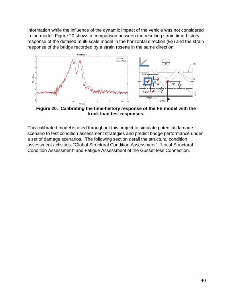
information while the influence of the dynamic impact of the vehicle was not considered in the model. Figure 20 shows a comparison between the resulting strain time-history response of the detailed multi-scale model in the horizontal direction (Ex) and the strain response of the bridge recorded by a strain rosette in the same direction.
Figure 20. Calibrating the time-history response of the FE model with the
truck load test responses.
This calibrated model is used throughout this project to simulate potential damage scenario to test condition assessment strategies and predict bridge performance under a set of damage scenarios. The following section detail the structural condition assessment activities: “Global Structural Condition Assessment”, “Local Structural Condition Assessment” and Fatigue Assessment of the Gusset-less Connection.

41
Global Structural Condition Assessment
The structural beam model of the bridge developed in SAP2000® was updated to reflect field observed structural behavior. The updating of the model was performed based on a parameter estimation procedure that changes the stiffness values of the structural members so that the error between the analytical model and the in-service bridge was minimized. For the Memorial Bridge, in particular, as the stiffness contribution of the gusset-less connections is a critical concern, the mechanical behavior of this innovative type of connection is not well-known. There are numerous techniques for structural model updating and structural condition assessment for which many of these methods require the modal properties of the structure, i.e., natural frequencies and mode shapes obtained by processing the monitoring data. The bridge excitation was categorized as ambient vibrations to pursue structural modal analysis.
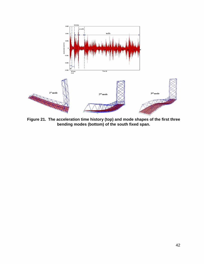
Figure 21 shows the acceleration time history captured by an accelerometer located on the top chord during a lift event as well as the corresponding mode shapes for the first three modes of the bridge. The natural frequencies are obtained by the frequency domain decomposition method. For this purpose, Hanning window with 60% overlap and bandpass Butterworth IIR filter with order 4 and lower cutoff frequency of 1 Hz and higher cutoff frequency of 5 Hz were used [Mehrkash et al., 2018]. The analytical and monitoring natural frequencies of the bridge are given in Table 8.
Table 8. The analytical (beam model) and identified natural frequencies of the first three bending modes of the south fixed span.
42
Figure 21. The acceleration time history (top) and mode shapes of the first three
bending modes (bottom) of the south fixed span.
43
Decision-making support
Structural investigations were performed to evaluate the impact of highly variable wind and wave load demands on the anchor points for the tidal turbine deployment system to the bridge pier [Yang et al., 2018]. The main contribution of this work was to provide a decision-making guide for turbine operation with response to environmental demands to ensure that the acceptable force, as determine through discussion with the bridge owner, is not exceeded.
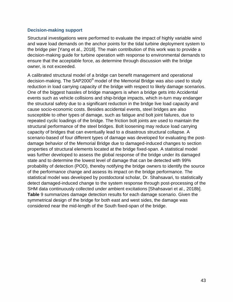
A calibrated structural model of a bridge can benefit management and operational decision-making. The SAP2000® model of the Memorial Bridge was also used to study reduction in load carrying capacity of the bridge with respect to likely damage scenarios. One of the biggest hassles of bridge managers is when a bridge gets into Accidental events such as vehicle collisions and ship-bridge impacts, which in-turn may endanger the structural safety due to a significant reduction in the bridge live load capacity and cause socio-economic costs. Besides accidental events, steel bridges are also susceptible to other types of damage, such as fatigue and bolt joint failures, due to repeated cyclic loadings of the bridge. The friction bolt joints are used to maintain the structural performance of the steel bridges. Bolt loosening may reduce load carrying capacity of bridges that can eventually lead to a disastrous structural collapse. A scenario-based of four different types of damage was developed for evaluating the post-damage behavior of the Memorial Bridge due to damaged-induced changes to section properties of structural elements located at the bridge fixed-span. A statistical model was further developed to assess the global response of the bridge under its damaged state and to determine the lowest level of damage that can be detected with 99% probability of detection (POD), thereby notifying the bridge owners to identify the source of the performance change and assess its impact on the bridge performance. The statistical model was developed by postdoctoral scholar, Dr. Shahsavari, to statistically detect damaged-induced change to the system response through post-processing of the SHM data continuously collected under ambient excitations [Shahsavari et al., 2018b]. Table 9 summarizes damage detection results for each damage scenario. Given the symmetrical design of the bridge for both east and west sides, the damage was considered near the mid-length of the South fixed-span of the bridge.
44
Table 9. Description of the simulated damage scenarios.
Damage Scenarios Damaged Members Reduction
Factor (%) Damage Detection
Algorithm
Detected Level (%) with 99%
POD
Truck accident
10, 20, 30, 40, 50, 60, 70, 80, 90
Control Chart Analysis 90
Vessel collision
10, 20, 30, 40, 50, 60, 70, 80, 90,
95
Control Chart Analysis 95
Fatigue
10, 20, 30, 40, 50, 60, 70, 80, 90,
95
Control Chart Analysis 95
Loose bolts
90 Control Chart Analysis 90
With the development of the system global response in the presence of damage, a live load rating factor, RF, was established to quantitatively perceive the structural performance of the bridge using the AASHTO Manual for Bridge Evaluation. The calculations were based on the design inventory level RF using an HL-93 live load and the Strength Design 1 load combination. An integrated decision-making protocol was developed to objectively analyze the SHM data to provide performance information for bridge owners due to likely damage scenarios and eventually indicate the need for more comprehensive and objective estimate on the bridge live load carrying capacity. A design inventory level greater than or equal to 1 (RF >= 1) implies that the bridge has adequate capacity to carry the AASHTO design load. Due to inherent limitation of the load rating approach for simultaneous consideration of axial and biaxial bending behaviors of the structural members, further investigations were proposed to reach a higher level of reliability based on the combined axial forces and biaxial flexural effects

45
according to the AASHTO Bridge Design Specifications. If the Interaction Ratio (IR) is lower than unit (IR<1) for all structural members, the bridge can remain in service and no further action is required.
Table 10 and Table 11 show the results of analytical investigations for both the simulated truck accident and vessel impact, quantified by load rating concept along with the AASHTO Bridge Design Specifications for combined axial and flexural effects in structural members. To predict whether the damaged members of the bridge due to the simulated damage satisfy the AASHTO design specifications for the combined interaction of axial forces and bending moments, the investigations were performed for different percentages of damage. As shown in Table 10, it was observed that the interaction ratio (IR) corresponding to the truck accident was less than 1 in all cases. These results were in good agreement with the corresponding load rating calculations, as the rating factor (RF) never dropped below 1.
Table 10. The rating factors and interaction ratios for the diagonal member damaged by truck accident.
Damage Scenario
Damaged Member
Capacity Reduction Factor (%)
Rating Factor (RF) Interaction Ratio (IR) Axial-
based Bending-
based
Truck accident Diagonal
0 7.92 16.68 0.26
10 6.78 15.67 0.27
20 6.09 15.63 0.27
30 5.40 15.57 0.28
40 4.71 15.50 0.39
50 4.02 15.44 0.42
60 3.33 15.32 0.47
70 2.63 15.18 0.54
80 1.92 14.89 0.64
90 1.18 13.94 0.85
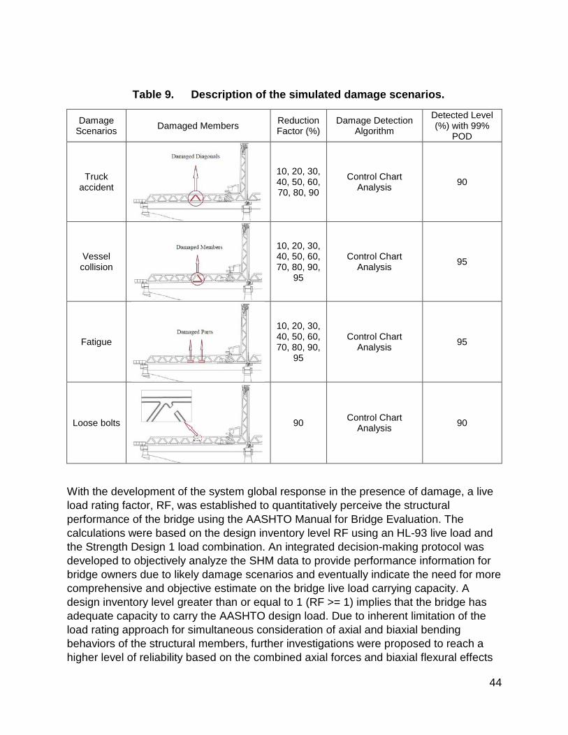
However, it was observed that the interaction ratio calculated for the combined axial tension and bending moments due to vessel collision did not satisfy the design specifications for severe incremental damage scenarios (see Table 11). According to the analytical results, while the highest percentage of damage (95% reduction) yields an interaction ration equal to 1.31, the axial-based load rating of damaged diagonals for this percentage of damage was shown to be 0.62. The interaction ratio was also investigated based on the damaged bottom chord for the vessel collision. As it is seen in Table 11, for damage cases greater than or equal to 80% reduction, the axial force and biaxial bending moment interaction ratios are greater than 1. However, the corresponding load rating drops below unit when the capacity reduction is greater than or equal to 90%. Therefore, the interaction ratio approach was found as a more
46
conservative method for the calculation of the load carrying capacity assessment particularly for members with significant bending and axial demands.
Table 11. The rating factors and interaction ratios for the diagonal member and bottom chord damaged by vessel collision.
Damage Scenario
Damaged Member
Capacity Reduction Factor (%)
Rating Factor (RF) Interaction Ratio
(IR) Axial-based
Bending-based
Vessel collision Diagonal
0 7.08 16.01 0.25
10 6.07 14.54 0.26
20 5.47 14.00 0.27
30 4.84 13.47 0.28
40 4.23 12.96 0.38
50 3.60 12.49 0.42
60 2.97 12.03 0.47
70 2.32 11.63 0.54
80 1.65 11.39 0.67
90 0.97 11.12 0.97
95 0.62 10.49 1.31
Vessel collision Bottom chord
0 13.19 5.89 0.35
10 11.14 5.10 0.37
20 9.93 4.67 0.47
30 8.71 4.23 0.52
40 7.50 3.77 0.57
50 6.29 3.29 0.65
60 5.09 2.76 0.75
70 3.88 2.18 0.90
80 2.68 1.51 1.14
90 1.46 0.70 1.67
95 0.82 0.21 2.35
Using the proposed decision-making protocol shown in Figure 22, load rating calculations determined that the bridge will be remained in service due to a truck accident simulated for the most extreme level of incremental damage. However, if the bridge experiences a vessel impact to its structural members as modeled in this work (damage levels greater than or equal to 90% reduction factor), deliberate actions should be taken immediately to reduce demand and repair damage. Potential actions include setting management strategies such as shutting down one or all lanes of the bridge, posting the bridge for less than legal loads, performing analytical investigations in order to repair or replace the damaged elements. Note that the load rating was not investigated for the other introduced damage scenarios of this work, i.e., fatigue and bolt loosening. This is because in the loose bolts case, one end of the diagonal member
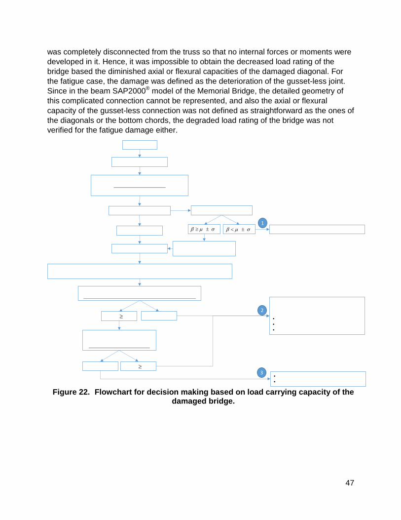
47
was completely disconnected from the truss so that no internal forces or moments were developed in it. Hence, it was impossible to obtain the decreased load rating of the bridge based the diminished axial or flexural capacities of the damaged diagonal. For the fatigue case, the damage was defined as the deterioration of the gusset-less joint. Since in the beam SAP2000® model of the Memorial Bridge, the detailed geometry of this complicated connection cannot be represented, and also the axial or flexural capacity of the gusset-less connection was not defined as straightforward as the ones of the diagonals or the bottom chords, the degraded load rating of the bridge was not verified for the fatigue damage either.
Figure 22. Flowchart for decision making based on load carrying capacity of the
damaged bridge.
•••
••
1
2
3≥
≥
β µ σ≥ ± β µ σ< ±

48
Local Structural Condition Assessment
Including Vertical Lift Excitations for Structural Condition Assessment of the Memorial Bridge Under the movement action of the movable bridges, the structural elements of the at the non-stationary span of the bridge sustain a unique excitation. These structural elements of the bridge are one of the less-accessible areas in these structures for inspection and instantiation. Due to the restriction of installation, the installed data acquisition systems may not properly report the health status of the structural components.
The vertical lift Memorial Bridge includes two towers for the lift operation of the middle span of the bridge. The SHM plan at the Memorial Bridge includes multiple data acquisition systems that are installed at the south tower of the bridge to capture the major lift excitations. The long-term collected SHM data of the tower informs a unique structural response during the lift action of the bridge. Even if the environmental variations and random outliers can cause variation in the recorded response, the trend of the structural response under the lift action can be well identified.
In Figure 23 and Figure 24, the acceleration and strain responses during the lift action is displayed for the located data acquisition systems at the tower, respectively. Also in Figure 24 the strain-time history response is shown during mid-span rise. This response is further applied for model verification and simulation of the lift action through an FE model.
Figure 23. The acceleration time-history response during the lift action of the
Memorial Bridge.
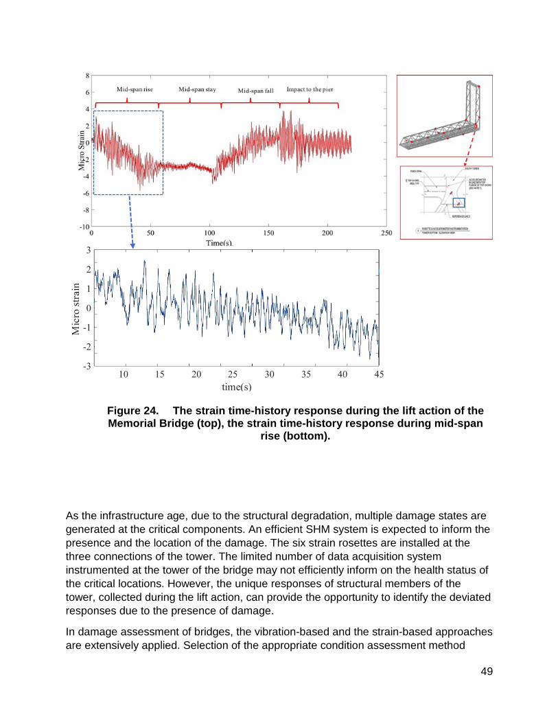
49
Figure 24. The strain time-history response during the lift action of the Memorial Bridge (top), the strain time-history response during mid-span
rise (bottom).
As the infrastructure age, due to the structural degradation, multiple damage states are generated at the critical components. An efficient SHM system is expected to inform the presence and the location of the damage. The six strain rosettes are installed at the three connections of the tower. The limited number of data acquisition system instrumented at the tower of the bridge may not efficiently inform on the health status of the critical locations. However, the unique responses of structural members of the tower, collected during the lift action, can provide the opportunity to identify the deviated responses due to the presence of damage.
In damage assessment of bridges, the vibration-based and the strain-based approaches are extensively applied. Selection of the appropriate condition assessment method

50
relies on the sensitivity analysis of the structural components. In the vibration-based damage detection method the changes in the dynamic characteristics of the bridge, including the mode shapes, are concerned. In detecting the local damages including the imperfection, weld defects due to lack of fusion or the surface cracks have a local property that may not to be distinguished through the changes in the global model responses. The small influence of the damage on the global performance of the structure may restrict the method for damage detection. The strain-based method relies on the changes of the local strain response at the vicinity of the instrumented location of the bridge. However, for large scale structures, the method may require the application of excessive strain gages that can report the local performance of the bridges. In addition, the damage prone areas are frequently less-accessible areas for instrumentation.
Through the investigation on the long-term collected data, it is realized that the vibration response responses of the tower during the lift action is significantly dependent on the mechanical system of the lift operation. Consequently, the vibration response of the tower can have a more variable property as compared to the strain response. The variability of the induced stresses under different traffic scenarios may impede to detect the damage-induced changes in the strain responses of the bridge. However, the exclusive strain responses of the tower during the lift action benefits to perform a condition assessment for the less-accessible structural members of the tower. The limited knowledge on the strain response of the tower, during the lift action, is completed using a validated numerical model of the bridge.
In this research, a global finite element model of the bridge is applied to achieve the numerical time-history response of the tower during the lift action [Mashayekhi and Santini-Bell, 2019]. Through the numerical model, the dynamic lift action is simulated. The details for simulating the lift mechanism is acquired through the as-built plans of the tower. The lift action of the midspan, is accompanied by the movement of the counterweights in a rail path, at the rear chords of the tower. As shown in Figure 25, to simulate the lift action, the rail paths are defined at the rear axles of the tower to apply the dynamic moving load. The intensity of the load is determined through calibrating the field collected strain response at the location of strain rosettes.

51
Figure 25. Simulating the lift action on the global model of the bridge using
the dynamic moving load along the tower.
In Figure 26, the field collected and the validated numerical strain responses of the model at the location of the specified strain rosette is shown. The displays response belongs to the upward movement of the midspan. The numerical model provides an identical strain time-history response (with the negative sign) for the downward action. Therefore, it this study, only the upward action is shown.
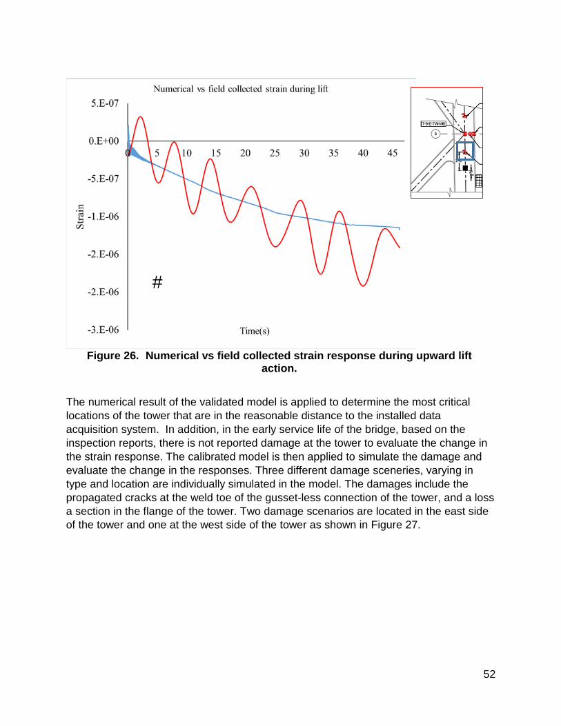
52
Figure 26. Numerical vs field collected strain response during upward lift action.
The numerical result of the validated model is applied to determine the most critical locations of the tower that are in the reasonable distance to the installed data acquisition system. In addition, in the early service life of the bridge, based on the inspection reports, there is not reported damage at the tower to evaluate the change in the strain response. The calibrated model is then applied to simulate the damage and evaluate the change in the responses. Three different damage sceneries, varying in type and location are individually simulated in the model. The damages include the propagated cracks at the weld toe of the gusset-less connection of the tower, and a loss a section in the flange of the tower. Two damage scenarios are located in the east side of the tower and one at the west side of the tower as shown in Figure 27.
#
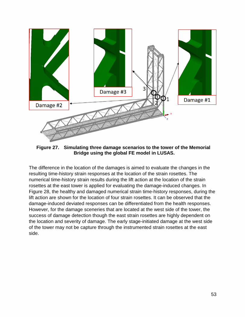
53
Figure 27. Simulating three damage scenarios to the tower of the Memorial
Bridge using the global FE model in LUSAS.
The difference in the location of the damages is aimed to evaluate the changes in the resulting time-history strain responses at the location of the strain rosettes. The numerical time-history strain results during the lift action at the location of the strain rosettes at the east tower is applied for evaluating the damage-induced changes. In Figure 28, the healthy and damaged numerical strain time-history responses, during the lift action are shown for the location of four strain rosettes. It can be observed that the damage-induced deviated responses can be differentiated from the health responses. However, for the damage sceneries that are located at the west side of the tower, the success of damage detection though the east strain rosettes are highly dependent on the location and severity of damage. The early stage-initiated damage at the west side of the tower may not be capture through the instrumented strain rosettes at the east side.
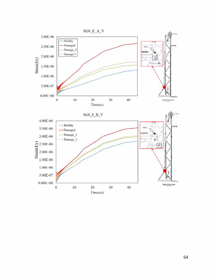
54
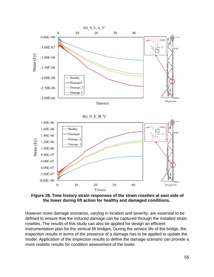
55
Figure 28. Time history strain responses of the strain rosettes at east side of
the tower during lift action for healthy and damaged conditions.
However more damage scenarios, varying in location and severity, are essential to be defined to ensure that the induced damage can be captured through the installed strain rosettes. The results of this study can also be applied for design an efficient instrumentation plan for the vertical lift bridges. During the service life of the bridge, the inspection results in terms of the presence of a damage has to be applied to update the model. Application of the inspection results to define the damage scenario can provide a more realistic results for condition assessment of the tower.

56
Fatigue Assessment of the Gusset-less Connections Using Field Collected Data and Analytical Model
The gusset-less connection at the Memorial Bridge consists of a complex geometric web and cold-bent flanges which are connected through a curved fillet weld with 5/8-inch thickness [Adams et al., 2016] The complex design of the connection, which is less studied in the existing fatigue design codes, motivates to perform a careful fatigue condition assessment. In addition, the gusset-less connection is applied to a truss bridge which is connected to multiple members in the planar and out-of-plane direction. The connected members can provide a complex loading condition for the gusset-less connection. Consequently, the traffic-induced stresses at the gusset-less connection can have a variable property due to the changes in the traffic loading system.
In this research study, the fatigue performance of the guest-less connection due to the unique geometry of the component and the complex applied loading condition is addressed. To perform the fatigue assessment, the field collected strain time-history responses of the strain rosettes, installed at the bottom gusset-less connection, are applied. The collected data helps to understand the variable amplitude stress ranges, which is induced under the traffic loads, at multiple locations of the component. In addition, through the FE global models developed in this study, the influence of the geometry on the fatigue performance of the component can be investigated. Fatigue assessment is performed using the nominal stress method and hotspot stress method. To measure the fatigue response, the assumption of the linear elastic relationship is valid to determine the stress responses. The stress responses are computed using the module of elasticity and the Poisson ratio, assumed for the design of the Memorial Bridge.
The nominal stress method
To measure the fatigue response, the appropriate S-N curve must be selected for the investigating structural component, shown in Figure 29. The categories of the welded structural components are defined from A to E. Also, the constant amplitude fatigue life (CAFL) that is specified for each fatigue category is the bottom threshold of the stress ranges, causing finite fatigue life. The novel gusset-less connection of the Memorial Bridge is not categorized among the recognized components existing in AASHTO fatigue categories. The Category C is considered for fatigue measurement of the fillet welds component, based on the designer’s assumptions and the AASHTO categorized specifications for the fillet welds [AASHTO 2012]. For the instrumented location of the connection, which are in-distance to the weld toe, the category B can be considered. The cumulative fatigue response (D) is measured for a selected period using the defined S-N curve’s specifications and the Miner’s rule [Miner, 1945] expressed in Equation (1).

57
=∑
(1)
where n and N are the number of the recorded cycles and number of remaining cycles to failure for each experienced stress range, respectively. In addition, in order to evaluate the trend of the accumulated fatigue response using a long period of data collection for the Memorial Bridge, the fatigue responses measured through Equation (1) are normalized. The normalization is performed using the Equation (2), where l is the number of the truck events in each period.
=
=∑ (2)
In an ideal period of data collection, the increase in the number of stress cycles under a steady flow of traffic loads can result in a smooth trend for the normalized fatigue response with some negligible fluctuations. However, there are multiple sources of variability in the collected data, that can induce a deviated fatigue response and therefore divergence on the trend of normalized fatigue response.
Figure 29. S-N curve of Fatigue categories by AASHTO [AASHTO, 2012].
Hot-spot stress fatigue assessment method
The hot-spot stress method does consider the local stress concentration due to the notch effect at the weld toe, while excluding the non-linear peak stress, as shown in Figure 30. The hot-spot stress can be determined by extrapolating the stress responses at the reference points (Figure 30). The distance of the reference points

58
to the weld toe depends on the type of the weld and size of the mesh in numerical models. For the investigating fillet weld toe, the reference points at the web of the connection, are located at the 0.4t and 1.0t (t is the thickness of the web) in a perpendicular distance to the weld toe, respectively, expressed in Equation 2. The stress responses at the reference points can be achieved using the numerical model and the fine mesh sizes. In the experimental efforts, the hotspot stresses are achieved by placement of the data acquisition system at the reference points (Radaj, 1990).
(2)
The ratio of the hot-spot stress range at the weld toe to the nominal stress is defined as the stress concentration factor (SCF) expressed in Equation 3. The SCF, which is frequently determined using the numerical models, can be multiplied to the nominal stresses to achieve the hot-spot stress without the requirement to the reference points. The SCF, in the previous studies, is applied for fatigue assessment of the structural components using the field collected nominal strain responses. Even if the variable amplitude traffic loads may result in multiple SCFs, a single SCF ratio is applied to the field collected responses [Niemi and Tanskanen1999].
(3)
The hot-spot stress method applies less S-N curves as compared to the nominal stress method. In IIW (international institute of welding), the fatigue classes (FAT class) and the associated S-N curves are expressed based on the type of the weld as well as the weld geometry. For the fillet welds, it is recommended to apply FAT 90 for the load carrying fillet welds and FAT 100 for the load carrying fillet welds [Fricke 2001]. In this research, regarding the performance of the weld at the gusset-less connection, FAT 100 is applied for fatigue assessment at the curved fillet welds.
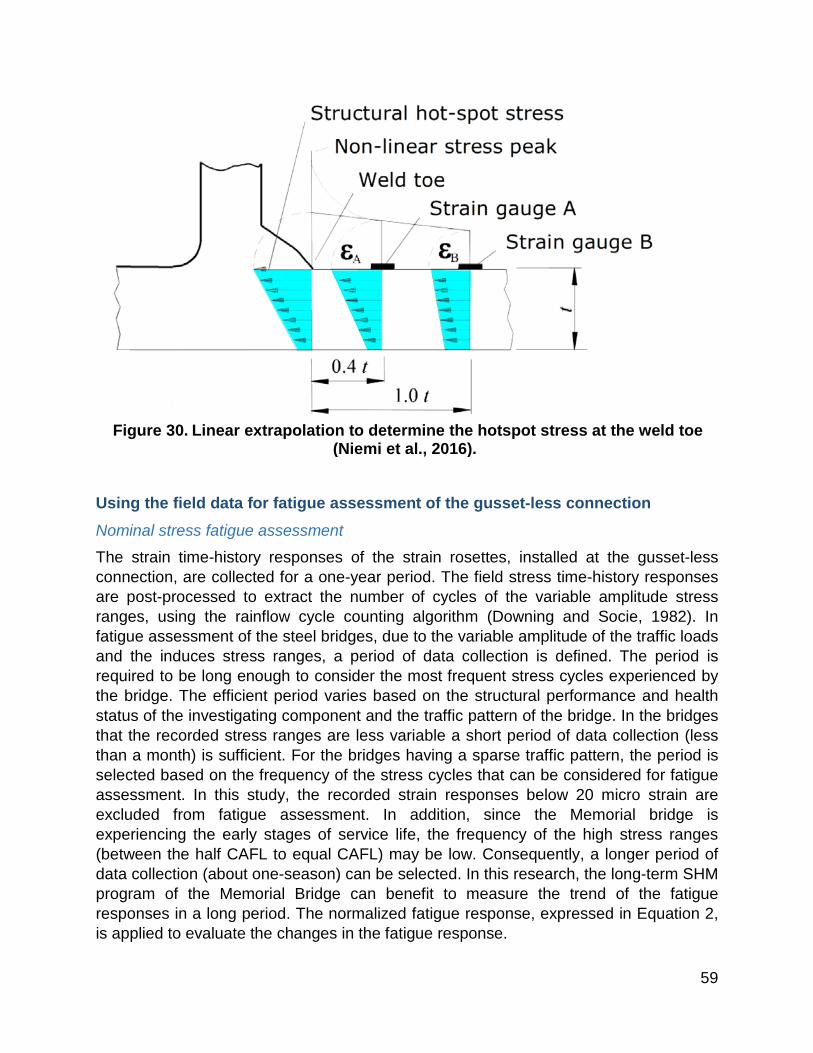
59
Figure 30. Linear extrapolation to determine the hotspot stress at the weld toe
(Niemi et al., 2016).
Using the field data for fatigue assessment of the gusset-less connection
Nominal stress fatigue assessment
The strain time-history responses of the strain rosettes, installed at the gusset-less connection, are collected for a one-year period. The field stress time-history responses are post-processed to extract the number of cycles of the variable amplitude stress ranges, using the rainflow cycle counting algorithm (Downing and Socie, 1982). In fatigue assessment of the steel bridges, due to the variable amplitude of the traffic loads and the induces stress ranges, a period of data collection is defined. The period is required to be long enough to consider the most frequent stress cycles experienced by the bridge. The efficient period varies based on the structural performance and health status of the investigating component and the traffic pattern of the bridge. In the bridges that the recorded stress ranges are less variable a short period of data collection (less than a month) is sufficient. For the bridges having a sparse traffic pattern, the period is selected based on the frequency of the stress cycles that can be considered for fatigue assessment. In this study, the recorded strain responses below 20 micro strain are excluded from fatigue assessment. In addition, since the Memorial bridge is experiencing the early stages of service life, the frequency of the high stress ranges (between the half CAFL to equal CAFL) may be low. Consequently, a longer period of data collection (about one-season) can be selected. In this research, the long-term SHM program of the Memorial Bridge can benefit to measure the trend of the fatigue responses in a long period. The normalized fatigue response, expressed in Equation 2, is applied to evaluate the changes in the fatigue response.
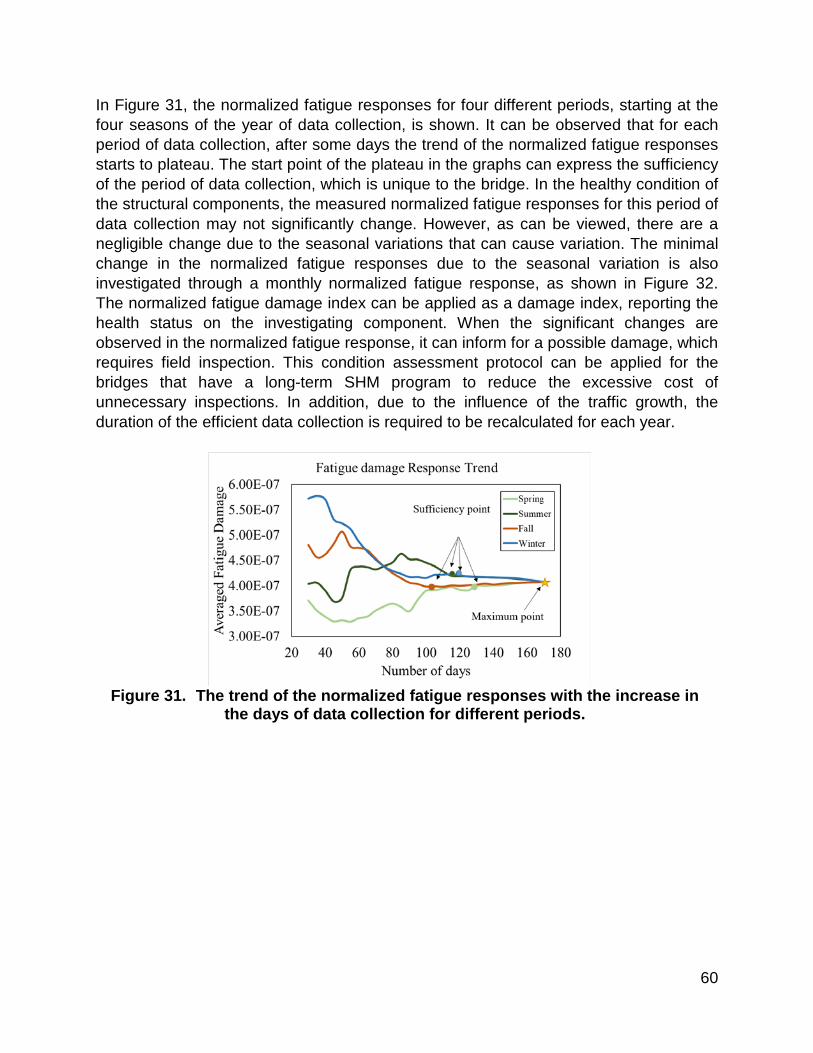
60
In Figure 31, the normalized fatigue responses for four different periods, starting at the four seasons of the year of data collection, is shown. It can be observed that for each period of data collection, after some days the trend of the normalized fatigue responses starts to plateau. The start point of the plateau in the graphs can express the sufficiency of the period of data collection, which is unique to the bridge. In the healthy condition of the structural components, the measured normalized fatigue responses for this period of data collection may not significantly change. However, as can be viewed, there are a negligible change due to the seasonal variations that can cause variation. The minimal change in the normalized fatigue responses due to the seasonal variation is also investigated through a monthly normalized fatigue response, as shown in Figure 32. The normalized fatigue damage index can be applied as a damage index, reporting the health status on the investigating component. When the significant changes are observed in the normalized fatigue response, it can inform for a possible damage, which requires field inspection. This condition assessment protocol can be applied for the bridges that have a long-term SHM program to reduce the excessive cost of unnecessary inspections. In addition, due to the influence of the traffic growth, the duration of the efficient data collection is required to be recalculated for each year.
Figure 31. The trend of the normalized fatigue responses with the increase in
the days of data collection for different periods.
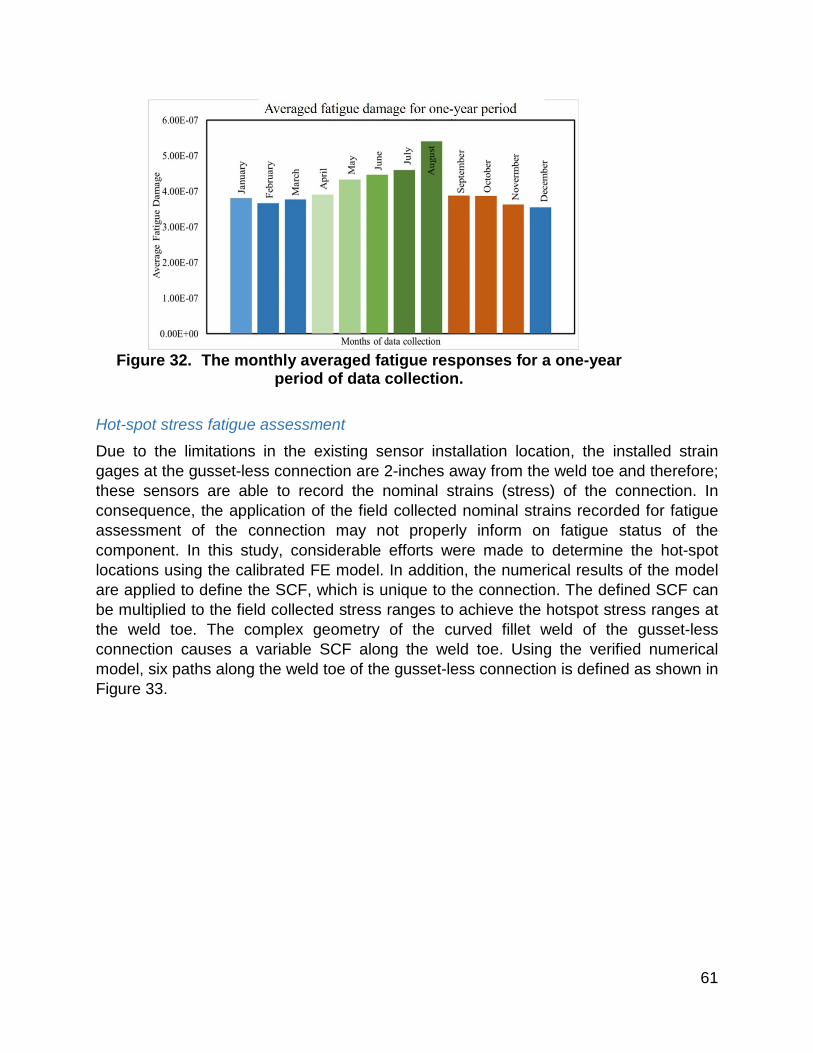
61
Figure 32. The monthly averaged fatigue responses for a one-year
period of data collection.
Hot-spot stress fatigue assessment
Due to the limitations in the existing sensor installation location, the installed strain gages at the gusset-less connection are 2-inches away from the weld toe and therefore; these sensors are able to record the nominal strains (stress) of the connection. In consequence, the application of the field collected nominal strains recorded for fatigue assessment of the connection may not properly inform on fatigue status of the component. In this study, considerable efforts were made to determine the hot-spot locations using the calibrated FE model. In addition, the numerical results of the model are applied to define the SCF, which is unique to the connection. The defined SCF can be multiplied to the field collected stress ranges to achieve the hotspot stress ranges at the weld toe. The complex geometry of the curved fillet weld of the gusset-less connection causes a variable SCF along the weld toe. Using the verified numerical model, six paths along the weld toe of the gusset-less connection is defined as shown in Figure 33.
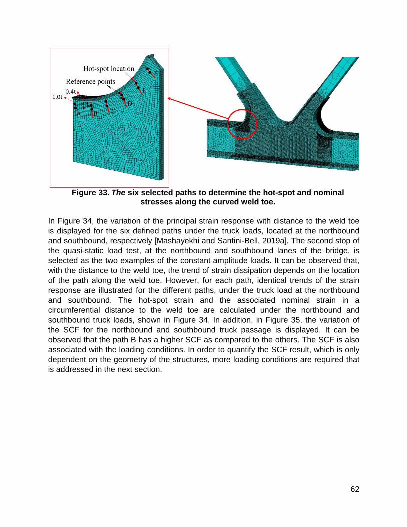
62
Figure 33. The six selected paths to determine the hot-spot and nominal
stresses along the curved weld toe. In Figure 34, the variation of the principal strain response with distance to the weld toe is displayed for the six defined paths under the truck loads, located at the northbound and southbound, respectively [Mashayekhi and Santini-Bell, 2019a]. The second stop of the quasi-static load test, at the northbound and southbound lanes of the bridge, is selected as the two examples of the constant amplitude loads. It can be observed that, with the distance to the weld toe, the trend of strain dissipation depends on the location of the path along the weld toe. However, for each path, identical trends of the strain response are illustrated for the different paths, under the truck load at the northbound and southbound. The hot-spot strain and the associated nominal strain in a circumferential distance to the weld toe are calculated under the northbound and southbound truck loads, shown in Figure 34. In addition, in Figure 35, the variation of the SCF for the northbound and southbound truck passage is displayed. It can be observed that the path B has a higher SCF as compared to the others. The SCF is also associated with the loading conditions. In order to quantify the SCF result, which is only dependent on the geometry of the structures, more loading conditions are required that is addressed in the next section.
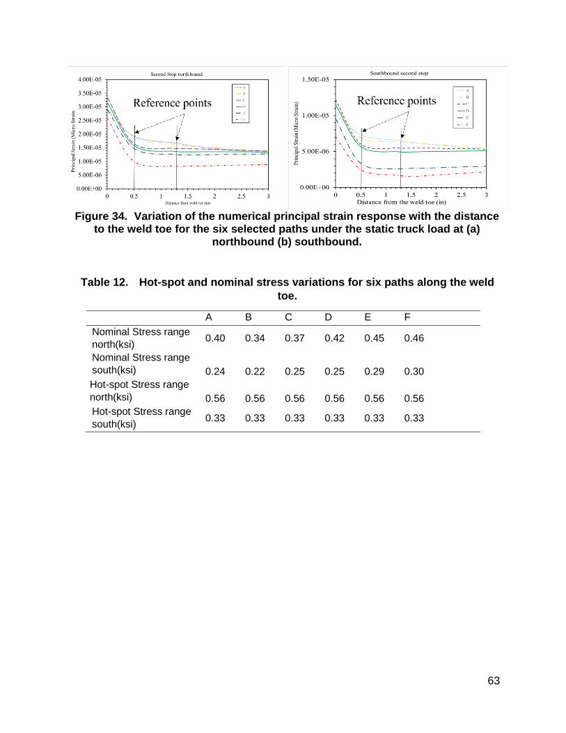
63
Figure 34. Variation of the numerical principal strain response with the distance
to the weld toe for the six selected paths under the static truck load at (a) northbound (b) southbound.
Table 12. Hot-spot and nominal stress variations for six paths along the weld toe.
A B C D E F Nominal Stress range north(ksi) 0.40 0.34 0.37 0.42 0.45 0.46
Nominal Stress range south(ksi) 0.24 0.22 0.25 0.25 0.29 0.30 Hot-spot Stress range north(ksi) 0.56 0.56 0.56 0.56 0.56 0.56 Hot-spot Stress range south(ksi) 0.33 0.33 0.33 0.33 0.33 0.33
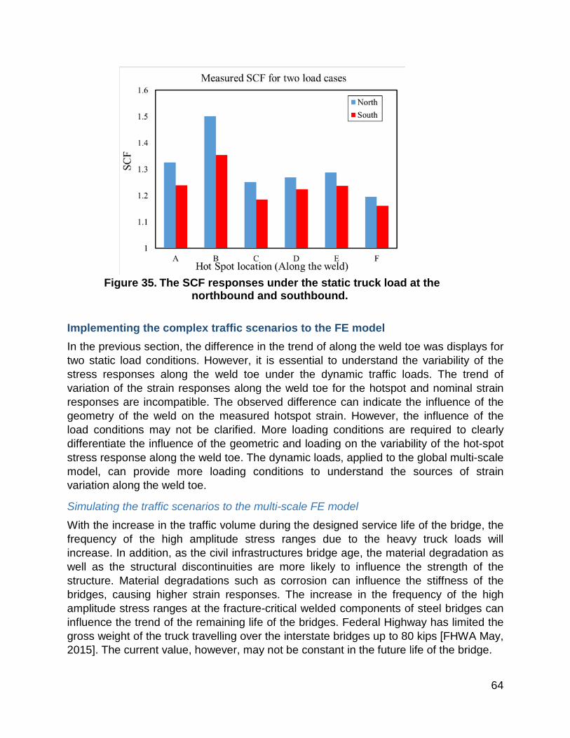
64
Figure 35. The SCF responses under the static truck load at the
northbound and southbound.
Implementing the complex traffic scenarios to the FE model
In the previous section, the difference in the trend of along the weld toe was displays for two static load conditions. However, it is essential to understand the variability of the stress responses along the weld toe under the dynamic traffic loads. The trend of variation of the strain responses along the weld toe for the hotspot and nominal strain responses are incompatible. The observed difference can indicate the influence of the geometry of the weld on the measured hotspot strain. However, the influence of the load conditions may not be clarified. More loading conditions are required to clearly differentiate the influence of the geometric and loading on the variability of the hot-spot stress response along the weld toe. The dynamic loads, applied to the global multi-scale model, can provide more loading conditions to understand the sources of strain variation along the weld toe.
Simulating the traffic scenarios to the multi-scale FE model
With the increase in the traffic volume during the designed service life of the bridge, the frequency of the high amplitude stress ranges due to the heavy truck loads will increase. In addition, as the civil infrastructures bridge age, the material degradation as well as the structural discontinuities are more likely to influence the strength of the structure. Material degradations such as corrosion can influence the stiffness of the bridges, causing higher strain responses. The increase in the frequency of the high amplitude stress ranges at the fracture-critical welded components of steel bridges can influence the trend of the remaining life of the bridges. Federal Highway has limited the gross weight of the truck travelling over the interstate bridges up to 80 kips [FHWA May, 2015]. The current value, however, may not be constant in the future life of the bridge.
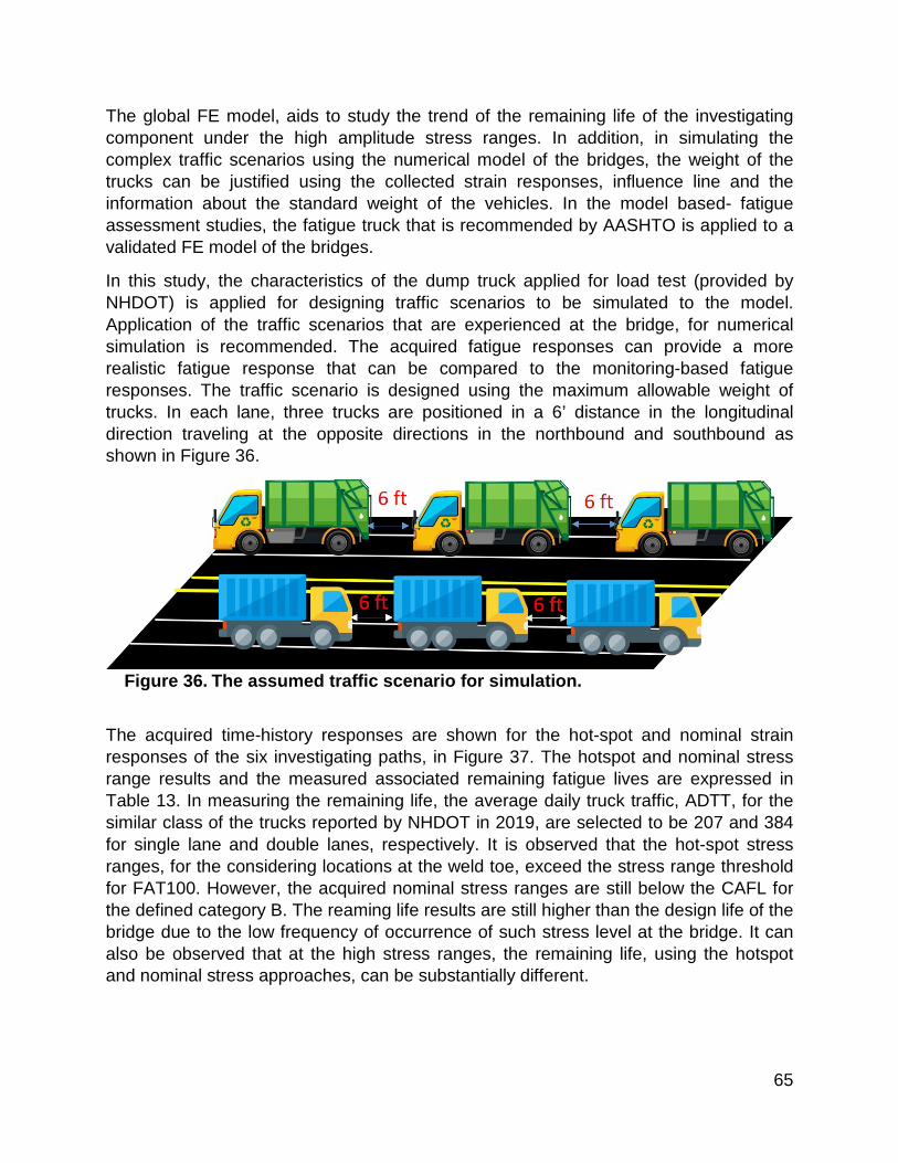
65
The global FE model, aids to study the trend of the remaining life of the investigating component under the high amplitude stress ranges. In addition, in simulating the complex traffic scenarios using the numerical model of the bridges, the weight of the trucks can be justified using the collected strain responses, influence line and the information about the standard weight of the vehicles. In the model based- fatigue assessment studies, the fatigue truck that is recommended by AASHTO is applied to a validated FE model of the bridges.
In this study, the characteristics of the dump truck applied for load test (provided by NHDOT) is applied for designing traffic scenarios to be simulated to the model. Application of the traffic scenarios that are experienced at the bridge, for numerical simulation is recommended. The acquired fatigue responses can provide a more realistic fatigue response that can be compared to the monitoring-based fatigue responses. The traffic scenario is designed using the maximum allowable weight of trucks. In each lane, three trucks are positioned in a 6’ distance in the longitudinal direction traveling at the opposite directions in the northbound and southbound as shown in Figure 36.
Figure 36. The assumed traffic scenario for simulation.
The acquired time-history responses are shown for the hot-spot and nominal strain responses of the six investigating paths, in Figure 37. The hotspot and nominal stress range results and the measured associated remaining fatigue lives are expressed in Table 13. In measuring the remaining life, the average daily truck traffic, ADTT, for the similar class of the trucks reported by NHDOT in 2019, are selected to be 207 and 384 for single lane and double lanes, respectively. It is observed that the hot-spot stress ranges, for the considering locations at the weld toe, exceed the stress range threshold for FAT100. However, the acquired nominal stress ranges are still below the CAFL for the defined category B. The reaming life results are still higher than the design life of the bridge due to the low frequency of occurrence of such stress level at the bridge. It can also be observed that at the high stress ranges, the remaining life, using the hotspot and nominal stress approaches, can be substantially different.
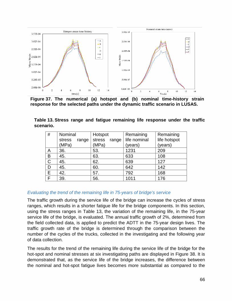
66
Figure 37. The numerical (a) hotspot and (b) nominal time-history strain response for the selected paths under the dynamic traffic scenario in LUSAS.
Table 13. Stress range and fatigue remaining life response under the traffic scenario.
# Nominal stress range (MPa)
Hotspot stress range (MPa)
Remaining life nominal (years)
Remaining life hotspot (years)
A 36. 53. 1231 209 B 45. 63. 633 108 C 45. 62. 639 127 D 45. 60. 642 142 E 42. 57. 792 168 F 39. 56. 1011 176
Evaluating the trend of the remaining life in 75-years of bridge’s service
The traffic growth during the service life of the bridge can increase the cycles of stress ranges, which results in a shorter fatigue life for the bridge components. In this section, using the stress ranges in Table 13, the variation of the remaining life, in the 75-year service life of the bridge, is evaluated. The annual traffic growth of 2%, determined from the field collected data, is applied to predict the ADTT in the 75-year design lives. The traffic growth rate of the bridge is determined through the comparison between the number of the cycles of the trucks, collected in the investigating and the following year of data collection.
The results for the trend of the remaining life during the service life of the bridge for the hot-spot and nominal stresses at six investigating paths are displayed in Figure 38. It is demonstrated that, as the service life of the bridge increases, the difference between the nominal and hot-spot fatigue lives becomes more substantial as compared to the
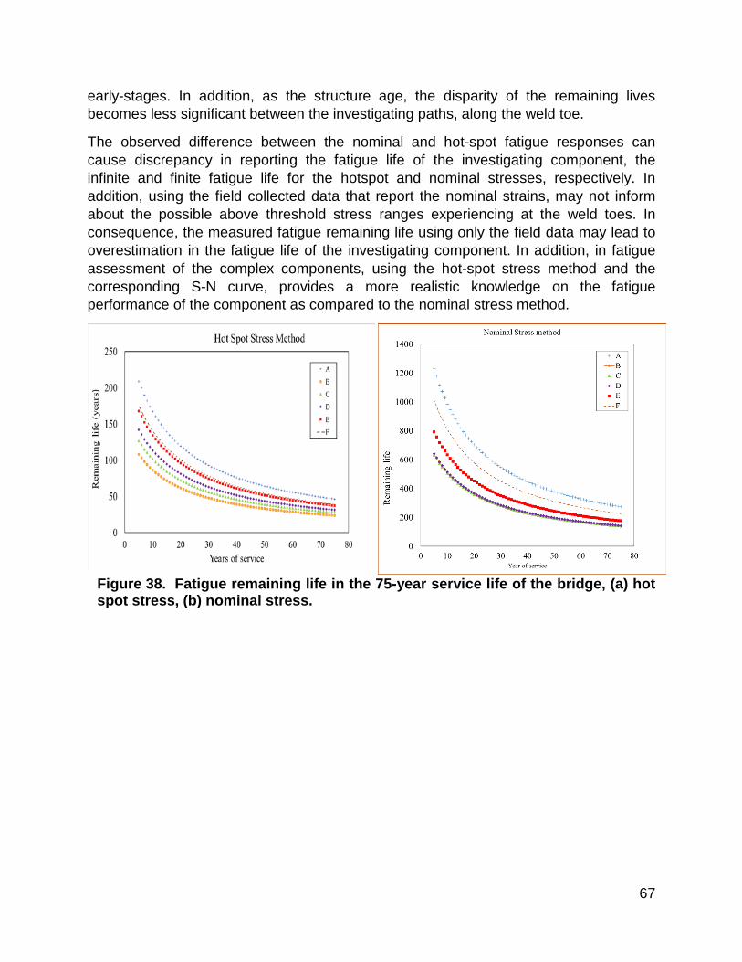
67
early-stages. In addition, as the structure age, the disparity of the remaining lives becomes less significant between the investigating paths, along the weld toe.
The observed difference between the nominal and hot-spot fatigue responses can cause discrepancy in reporting the fatigue life of the investigating component, the infinite and finite fatigue life for the hotspot and nominal stresses, respectively. In addition, using the field collected data that report the nominal strains, may not inform about the possible above threshold stress ranges experiencing at the weld toes. In consequence, the measured fatigue remaining life using only the field data may lead to overestimation in the fatigue life of the investigating component. In addition, in fatigue assessment of the complex components, using the hot-spot stress method and the corresponding S-N curve, provides a more realistic knowledge on the fatigue performance of the component as compared to the nominal stress method.
Figure 38. Fatigue remaining life in the 75-year service life of the bridge, (a) hot spot stress, (b) nominal stress.

68
Schedule
Each task listed in the project timeline had an integral role in the development of a significant advancement in bridge design, traffic and construction, management, and bridge maintenance, see Table 14. During the life of this project, the benefit of a smart technology for monitoring and management of transportation infrastructure will be communicated to stakeholders and decision-making through the state for possible adoption of these technologies to appropriate project. Part of the dissemination plan is workshops that will be conducted in cooperation with the UNH-Technology Transfer Center during each project year to share the benefits and performance of the innovations.
Table 14. Living Bridge project timeline.
Year 1 Install sensor network for structural, traffic and environment/estuary monitoring system,
calibrate bridge finite element model from field data, record baseline data Year 2 Monitor, record and assess performance data, for structural integrity, traffic
and environmental impact. Year 3 Assessment of the innovations and change in infrastructure management
procedures at the NHDOT.
Cost
This cost benefit of this project is the objective performance measure provided by the collected structural health monitoring data. This saving can be realized through directly visual inspection that focus on high-stress area as predicted by field-verified structural models or preventive maintenance procedure for lift balancing when the tower accelerations exhibit asymmetric behavior.
This cost saving will materialize only when the bridge asset management and operation procedures are designed to accept structural health monitoring information for decision-making and deterioration modeling and prediction.
Quality
As previously discussed, using traditional project delivery techniques the (insert recipient or subrecipient) would have (reiterate “baseline” process). However, using this innovation we could (insert applicable discussion on; constructability, materials control, elimination of joints, etc. and how that impacts long term service life of infrastructure). (Since this report is due within six months of project completion, there likely is not time for a full assessment of the “quality” of the final product so extrapolation from baseline of comparable facilities delivered using conventional methods will be necessary for comparison purposes.)

69
User Costs
The implementation of structural health monitoring on critical elements, such as fracture critical or fatigue-prone connection can reduced life cycle costs. This data, as shown above, can capture the fatigue performance of the element and be used to validate analytical models, both structural and mathematical, to predict the impact of simulated deterioration or damage on fatigue performance and structural performance.
User Satisfaction
NA
Project Outcomes and Lessons Learned Through this project, the NHDOT gained valuable insights about the innovative SHM techniques and technologies used.
Recommendations and Implementation
Recommendations
For beam modeling of gusset-less connection in SAP2000®, adding bracing members to the joint region is recommended as the most efficient modeling approach. Such a modeling technique can increase the rotational stiffness of the gusset-less connection in the beam modeling and makes the simplified beam model of the truss more representative of the real structure. It is also recommended that in addition to estimation of the Young’s modulus of the bracing members, their mass is updated as well.
• For system identification, the existing instrumentation (accelerometers) seems to be sufficient for extraction of natural frequencies of the structure from the frequency response functions of monitoring data. However, the accuracy of identified mode shapes is not satisfactory. If more accurate mode shapes are required, it is recommended to install more accelerometers on the bridge.
• It was demonstrated that the wavelet packet-based damage detection is a robust tool for structural condition assessment of the bridge. For utilizing this technique, the vibration of the bridge due to impact of the lift span on the pier is analyzed. At this point, there is not any straightforward measurement equipment for impact load identification that emits a transient wave to the fixed span right after lowering. It is recommended that some appropriate measuring protocol to be planned for the impact load identification of the lift span on the pier.
• As the bridge is structurally overdesigned, the effects of rigidity of the connections in the 3D model of the structure is overshadowed by the structural indeterminacy of the bridge. It is recommended that the focus of monitoring system to be shifted to some more vulnerable parts of the bridge.

70
• Damping of the bridge is unknown and may raise a lot of questions. For vibration analysis of the bridge, the damping can be a critical factor which need to be estimated for future condition assessment plans.
• Interaction of tower and span may be an important issue for vibration analysis of the bridge. Particularly, as the number of sensors on the tower are less than the ones on the span, it seems that the sensors of the span may not be sufficient for detection of potential damage cases of the tower. Therefore, it is recommended to add some more sensors on the tower to monitor the health of tower with more confidence.
• The existing instrumentation of the bridge showed good capability for damage detection of the bridge. It is recommended that the current instrumentation to be kept for future damage detection plans.
• Because of the connection of bottom chords of the bridge to the floor beams and deck, the damage of bottom chords, especially due to vessel accident, does not affect the structural behavior of the bridge considerably. If the budget of the future projects allows to make the sensor grid denser, it is recommended to add the new sensors to the top chords.
• As the south end of the south fixed span is the most vulnerable part of the instrumented span, it is recommended to inspect the truss members of the Portsmouth side abutment more frequently.
• Using the multi-scale modeling method, helps to perform complex analyses with significant reduction in computation time. However, this modeling approach requires an intuition about the structural performance of the elements. Selecting the type of the elements and the number of nodal degrees of freedom (DOF) and size of the mesh are defined based on the structural performance of the members. It is recommended to make the initial assumption with lower dimension of elements with large mesh sizes. The final adjustments can be performed for model validation to increase the accuracy of the response.
• In modeling the long members application of higher dimension elements can increase the number of nodal DOFs and the computation time. However, modeling the members that transfer a considerable load, such as floor beam, may result in concentrated stress at the connecting member to the end of beam. In this case, it is recommended that to apply higher dimension element (shell element) at the end section of the beam to reduce the stress concentration.
• In developing the multi-scale model, the location of interface points that couples the higher to lower dimension of elements have to determined properly. The interface point is required to be in a reasonable distance to the concentrated locations of the structural components. In the modeling large scale structures having complex geometry, defining the optimum location for the interface point can play a significant role stiffness of the structure and subsequently the numerical results. It is recommended to make an initial assumption for the interface point in creating a multi-scale model and then adjust the location in the calibration process of the mode.

71
• In the three investigating locations of the accelerometers of the bridge, it is illustrated that the temperature variation has a significant impact on the variability of the vibration response. To create a comprehensive model, which can predict the nonlinear relationship of the temperature to the vibration responses, a wider range of temperature and wind variations can be beneficial. The required range of environmental data for model prediction is significantly dependent on the climate conditions at the area of study. In Portsmouth, NH, less frequent lift action and traffic volume is recorded in the below freezing period. However, it is recommended to consider the vibration response as well as the environmental data of the below freezing days, in developing an efficient ANN model.
• However more damage scenarios, varying in location and severity, are essential to be defined to ensure that the induced damage can be captured through the installed strain rosettes. The results of this study can also be applied for design an efficient instrumentation plan for the vertical lift bridges. During the service life of the bridge, the inspection results in terms of the presence of a damage has to be applied to update the model. Application of the inspection results to define the damage scenario can provide a more realistic results for condition assessment of the tower. The detected damage can be simulated to the model to update the condition of the model for evaluating the influence of the damage on the critical parts of the structure.
• In this study, the fatigue assessment is performed for the healthy condition of the bridges. The presence of the fatigue cracks and the material degradations at multiple locations of the structural components will increase the variability of stress ranges and the fatigue responses of the component. Particularly, the fatigue responses at the stress concentrated areas close to the initiated crack can be significantly higher than the nominal fatigue responses in a sizeable distance to the crack location. differences, that is not considered in the results. The created multi-scale model, in this study, also can benefit to study the fatigue performance of the welded structural components having structural discontinuities such as imperfections in the weld or the fatigue crack at the weld toe (or root). It is recommended for future studies, simulate the possible crack in the model and evaluate the difference between the nominal fatigue response to the crack-induced fatigue response.
Status of Implementation and Adoption
Since the completion of Living Bridge Project, the research team and the NHDOT has undertaken the following activities to implement structural health monitoring into our standard operating procedures as a significant improvement from our traditional practice for similar type projects: (1) Inform the Bridge Design and Bridge Maintenance Bureaus of the potential benefit for structural health monitoring bridge decision-making through engagement on the project advisory board, (2) Provide a fatigue assessment using the traditional AASHTO fatigue life prediction and the hot-spot stress fatigue life prediction at the Memorial Bridge to demonstrate the operational benefit of SHM data, (3) Provide a mechanism for NHDOT employees to determine if a project is a candidate for SHM through communication with UNH research team and results of this project.

72
Appendix
Technology Transfer
• Adams, T., Mashayekhizadeh, M., Santini-Bell, E., Wosnik, M., Baldwin, K., Fu, T. (2017) “Structural Response Monitoring of a Vertical Lift Truss Bridge”, 96th Transportation Research Board Annual Meeting Compendium of Papers, Washington D.C, January 8-12, 17-06353.
• Fischer, F. (2018). “Design and Fabrication of a Specimen and Experimental Setup for Fatigue Testing of a Gusset-less Bridge Connection.” M.Sc. thesis, University of New Hampshire, NH, USA.
• Manning, T. E. (2017). “Enhanced in-service condition assessment of bridges using GoPro® cameras,” M. Sc. Thesis, University of New Hampshire, NH, USA.
• Mashayekhizadeh, M., Adams,T., Yang,C., Gagnon,I., Wosnik,M., Baldwin, K., Santini-Bell, E. (2016) ”Structural Health Monitoring and Design Verification of Tidal Turbine Support Structure”, Proceedings of 75th ASNT Annual Conference, Long Beach, CA.
• Mashayekhizadeh, M., Santini-Bell, E. and Adams, T. (2017). “Instrumentation and Structural Health Monitoring of a Vertical Lift Bridge”, Proceedings of the 26th ASNT Research Symposium, Jacksonville, FL.
• Mashayekhizadeh, M., Santini-Bell, E. (2018) “Influence of temperature in vibration-based structural health monitoring of a vertical lift bridge”, 27th ASNT Research Symposium, Orlando, FL.
• Mashayekhizadeh, M., Mehrkash, M., Shahsavari, V., and Santini-Bell, E. (2018). “Multi-scale finite element model development for long-term condition assessment of vertical lift bridge,” ASCE Structures Congress, Fort Worth, TX.
• Mashayekhizadeh, M., Bell, E. (2018) “Data Validated Multi-Scale Finite Element Modeling Protocol for Complex Connections of a Movable Bridge”, Engineering Mechanics Institute Conference, Cambridge, MA.
• Mashayekhi, M. and Santini-Bell, E.* (2018). “Developing three-dimensional multi-scale finite element model for in-plane service performance assessment of bridges” Computer-Aided Civil and Infrastructure Engineering, 34(5), 385-403.
• Mashayekhi, M., Santini-Bell, E. (2019) “Including Environmental and Vertical Lift Excitations for Structural Condition Assessment of a Gusset-less Truss Bridge”, 28th ASNT Research Symposium, Garden Grove, CA.
• Mashayekhi, M., Santini-Bell, E. (2019a) “Fatigue assessment of the gusset-less connection using field data and numerical model” 10th New York City Bridge Conference, New York.
• Mashayekhi, M., Santini-Bell, E. (2019b) “Detection of damage-induced fatigue response based on structural health monitoring data of in-service steel bridges using Artificial Neural Network” 12th International Workshop on Structural Health

73
Monitoring, IWSHM, Stanford, CA.
• McGeehan, D., Zargar Shoushtari, S., Medina, R. and Santini-Bell, E. (2019). “Comparison of multiple strain measurement techniques to characterize the behavior of an experimental fatigue test.” 98th Annual Meeting of Transportation Research Board, Washington D.C.
• McGeehan, D. W. (2018). “Experimental Evaluation of Fatigue Test Setup for a Gusset-less Truss Connection.” M.Sc. thesis, University of New Hampshire, NH, USA.
• Mehrkash, M., and Santini-Bell, E. (2018a). “Modeling and characterization of complicated connections in structural and mechanical systems as applied to a gusset-less truss connection,” 97th Annual Meeting of Transportation Research Board, Washington D.C.
• Mehrkash, M., Shahsavari, M., and Santini-Bell, E. (2018). “Instrumentation sufficiency of a vertical lift bridge for modal system identification by frequency domain analysis,” Engineering Mechanics Institute Conference, Cambridge, MA.
• Mehrkash, M., and Santini-Bell, E. (2018b). “System identification of a bridge gusset-less connection by simplified and detailed local analytical models,” NDE/NDT for Highway and Bridges: Structural Materials Technology and the International Symposium on Non-Destructive Testing in Civil Engineering, New Brunswick, NJ.
• Mehrkash, M., and Santini-Bell, E. (2019a). “Finite element model updating of the UCF Grid benchmark connections using experimental modal data,” 37th International Modal Analysis Conference, Orlando, FL.
• Mehrkash, M., Shahsavari, V., and Santini-Bell, E. (2019). “Instrumentation plan verification for damage detection of a vertical lift steel truss bridge,” SPIE Smart Structures and Nondestructive Evaluation, Denver, CO.
• Mehrkash, M., and Santini-Bell, E. (2019b). “Local condition assessment and damage detection of gusset-less connections used in a vertical lift truss bridge,” 9th International Conference on Structural Health Monitoring of Intelligent Infrastructure, St. Louis, MO.
• Nash, T. P. (2016). “An objective protocol for movable bridge operation in high-wind events based on hybrid analyses by European and American design code,” M.Sc. Thesis, University of New Hampshire. NH, USA.
• Nash, T., Santini-Bell, E., Mehrkash, M., and Shahsavari, V. (2018), “An objective decision-making protocol for lift bridge operation subjected to high wind loads,” Engineering Mechanics Institute Conference, Cambridge, MA.\
• Santini-Bell, E., Mashayekhizadeh, M., Adams, T., Nash, T. (2017) “Structural Monitoring to Support Decision-Making on the A Vertical Lift Bridge”, Proceedings of the Twelfth International Conference on Structural Safety and Reliability (ICOSSAR), Vienna, 2386-2395.

74
• Shahsavari, V., Mehrkash, M., and Santini-Bell, E. (2018a). “Structural health monitoring of a vertical lift bridge using vibration data,” 27th ASNT Research Symposium, Orlando, FL.
• Shahsavari, V., Mehrkash, M., and Santini-Bell, E. (2018b). “Effect of damaged structural members on performance degradation of a vertical lift truss bridge,” ASNT Annual Conference, Houston, TX.
• Shahsavari, V., Mehrkash, M., and Santini-Bell, E. (2019). Progressive damage assessment and vulnerability evaluation of a vertical lift steel gusset-less truss bridge by wavelet analysis, 28th ASNT Research Symposium, Garden Grove, CA.
• Yang, C., Santini-Bell, E., Shahsavari, V., and Mehrkash, M. (2018). “Probability-based demand evaluation of the bridge tidal turbine deployment system subject to environmental events, Engineering Mechanics Institute Conference,” Cambridge, MA.
User Satisfaction Survey
Through NSF funding for a complimentary Living Bridge project, the research team used the Granite State poll to collect data on how New Hampshire residents view the state of the transportation infrastructure in New Hampshire. The Granite State Poll collected the county of residence, age and education level along with several other identifies factors for all respondents. The question asked was “The condition of basic highway, bridge, & transportation infrastructure in New Hampshire today is (a) Better than 10 or 20 years ago? (b) Worse than 10 or 20 years ago? Or (c) About the same as 10 or 20 years ago?. The possible answers were presented in a random order. Figure 39 displays the results. A full report on the survey results are available https://scholars.unh.edu/carsey/318/
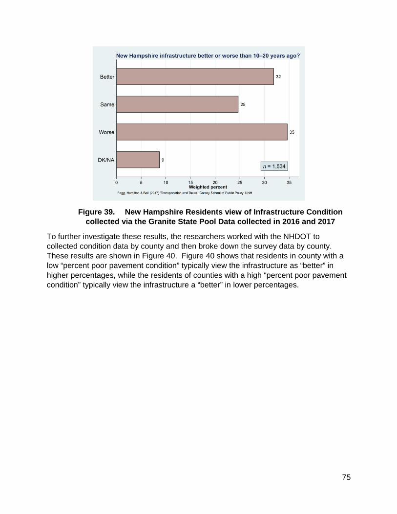
75
Figure 39. New Hampshire Residents view of Infrastructure Condition collected via the Granite State Pool Data collected in 2016 and 2017
To further investigate these results, the researchers worked with the NHDOT to collected condition data by county and then broke down the survey data by county. These results are shown in Figure 40. Figure 40 shows that residents in county with a low “percent poor pavement condition” typically view the infrastructure as “better” in higher percentages, while the residents of counties with a high “percent poor pavement condition” typically view the infrastructure a “better” in lower percentages.
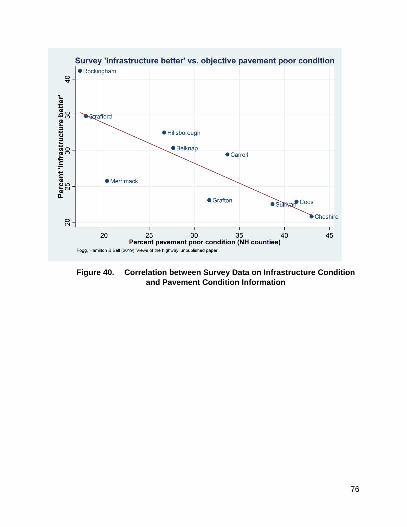
76
Figure 40. Correlation between Survey Data on Infrastructure Condition and Pavement Condition Information

77
Web Resources
The instrumentation plan and select historic structural health monitoring data are available at the project website, livingbridge.unh.edu.
This project has been highlighted in several news media outlets and multi-media venues:
• Living Bridge Project shows off potential of "smart" infrastructure - Science Nation: https://www.nsf.gov/news/special_reports/science_nation/livingbridge.jsp
• University Of New Hampshire, NSF, Others Collaborate On “Smart” Bridge Project Seacoast Online (NH) (6/4) reports, “Engineers at the University of New Hampshire designed a living laboratory on the iconic Memorial Bridge, which could change how infrastructure is viewed.” Memorial Bridge “was outfitted with data sensors that transformed it into a self-diagnosing, self-reporting ‘smart’ bridge that captures a range of information from the health of the span to the environment around it.” The project “is a collaborative effort led by UNH with the New Hampshire Department of Transportation, National Science Foundation and US Department of Energy.”
• https://www.fosters.com/news/20190604/unh-engineers-bring-memorial-bridge-to-life-with-data-sensors
• https://www.unionleader.com/news/education/portsmouth-s-memorial-bridge-serves-double-duty-as-unh-research/article_c5ee1e0d-c207-584e-b757-6319b1cfa490.html
• :https://www.wcvb.com/article/a-local-shrimp-growing-project-is-generating-income-for-farmers-far-from-the-ocean/23713329
• https://scienmag.com/its-alive-unh-researchers-create-innovative-living-bridge/ • https://www.eurekalert.org/pub_releases/2019-06/uonh-iau060419.php • https://www.nhbr.com/unh-researchers-create-living-memorial-bridge/ • https://www.expresscomputer.in/iot/embedded-with-sensors-engineers-create-
self-diagnosing-self-reporting-smart-bridge/36574/ • https://bioengineer.org/its-alive-unh-researchers-create-innovative-living-bridge/ • https://phys.org/news/2019-06-alive-bridge.html • https://www.ecnmag.com/videos/2019/06/its-alive-unh-researchers-create-
innovative-living-bridge • http://www.connectivity4ir.co.uk/article/171373/Engineers-at-the-University-of-
New-Hampshire-create-a--living--bridge.aspx • http://scienstack.com/its-alive-unh-researchers-create-innovative-living-bridge/ • https://www.techexplorist.com/engineers-transformed-iconic-bridge-living-
laboratory/23935/ • https://www.wmur.com/article/sensors-placed-on-memorial-bridge-by-unh-
engineers-collecting-structure-environment-data/27735886 • http://www.scitechreport.com/cluster52800440/ • https://newatlas.com/memorial-bridge-living-laboratory/60039/

78
• https://www.citylab.com/life/2016/11/living-bridge-data-smart-infrastructure-new-hampshire-memorial-bridge/508040/
References
• Adams, T., Mashayekhizadeh, M., Santini-Bell, E., Wosnik, M., Baldwin, K., Fu, T. (2017) “Structural Response Monitoring of a Vertical Lift Truss Bridge”, 96th Transportation Research Board Annual Meeting Compendium of Papers, Washington D.C, January 8-12, 17-06353.
• AASHTO. (2012). “AASHTO LRFD Bridge Design Specifications. American Association of State Highway and Transportation Officials,” Washington, D.C.
• Downing S.D., Socie D.F. (1982). “Simple rainflow counting algorithms,” International Journal of Fatigue 4 (1), 31-40.
• FHWA. (2015). “Compilation of Existing State Truck Size and Weight Limit Laws,” Report to Congress. Washington, D.C.
• Fricke, W. (2001) “Recommended Hot Spot Analysis Procedure for Structural Details of FPSOs And Ships Based on Round-Robin FE Analyses,” The Eleventh International Offshore and Polar Engineering Conference. Stavanger, Norway.
• Fischer, F. (2018). “Design and Fabrication of a Specimen and Experimental Setup for Fatigue Testing of a Gusset-less Bridge Connection.” M.Sc. thesis, University of New Hampshire, NH, USA.
• Manning, T. E. (2017). “Enhanced in-service condition assessment of bridges using GoPro® cameras,” M. Sc. Thesis, University of New Hampshire.
• Mashayekhizadeh, M., Adams,T., Yang,C., Gagnon,I., Wosnik,M., Baldwin, K., Santini-Bell, E. (2016) ”Structural Health Monitoring and Design Verification of Tidal Turbine Support Structure”, Proceedings of 75th ASNT Annual Conference, Long Beach, CA.
• Mashayekhizadeh, M., Santini-Bell, E. and Adams, T. (2017). “Instrumentation and Structural Health Monitoring of a Vertical Lift Bridge”, Proceedings of the 26th ASNT Research Symposium, Jacksonville, FL.
• Santini-Bell, E., Mashayekhizadeh, M., Adams, T., Nash, T. (2017) “Structural Monitoring to Support Decision-Making on the A Vertical Lift Bridge”, Proceedings of the Twelfth International Conference on Structural Safety and Reliability (ICOSSAR), Vienna, 2386-2395.
• Mashayekhizadeh, M., Santini-Bell, E. (2018) “Influence of temperature in vibration-based structural health monitoring of a vertical lift bridge”, 27th ASNT Research Symposium, Orlando, FL.

79
• Mashayekhizadeh, M., Mehrkash, M., Shahsavari, V., and Santini-Bell, E. (2018). “Multi-scale finite element model development for long-term condition assessment of vertical lift bridge,” ASCE Structures Congress, Fort Worth, TX.
• Mashayekhizadeh, M., Bell, E. (2018) “Data Validated Multi-Scale Finite Element Modeling Protocol for Complex Connections of a Movable Bridge”, Engineering Mechanics Institute Conference, Cambridge, MA.
• Mashayekhi, M. and Santini-Bell, E.* (2018). “Developing three-dimensional multi-scale finite element model for in-plane service performance assessment of bridges” Computer-Aided Civil and Infrastructure Engineering, 34(5), 385-403.
• Mashayekhi, M., Santini-Bell, E. (2019) “Including Environmental and Vertical Lift Excitations for Structural Condition Assessment of a Gusset-less Truss Bridge”, 28th ASNT Research Symposium, Garden Grove, CA.
• Mashayekhi, M., Santini-Bell, E. (2019a) “Fatigue assessment of the gusset-less connection using field data and numerical model” 10th New York City Bridge Conference, New York.
• Mashayekhi, M., Santini-Bell, E. (2019b) “Detection of damage-induced fatigue response based on structural health monitoring data of in-service steel bridges using Artificial Neural Network” 12th International Workshop on Structural Health Monitoring, IWSHM, Stanford, CA.
• McGeehan, D., Zargar Shoushtari, S., Medina, R. and Santini-Bell, E. (2019). “Comparison of multiple strain measurement techniques to characterize the behavior of an experimental fatigue test.” 98th Annual Meeting of Transportation Research Board, Washington D.C.
• McGeehan, D. W. (2018). “Experimental Evaluation of Fatigue Test Setup for a Gusset-less Truss Connection.” M.Sc. thesis, University of New Hampshire, NH, USA.
• Mehrkash, M., and Santini-Bell, E. (2018a). “Modeling and characterization of complicated connections in structural and mechanical systems as applied to a gusset-less truss connection,” 97th Annual Meeting of Transportation Research Board, Washington D.C.
• Mehrkash, M., Shahsavari, M., and Santini-Bell, E. (2018). “Instrumentation sufficiency of a vertical lift bridge for modal system identification by frequency domain analysis,” Engineering Mechanics Institute Conference, Cambridge, MA.
• Mehrkash, M., and Santini-Bell, E. (2018b). “System identification of a bridge gusset-less connection by simplified and detailed local analytical models,” NDE/NDT for Highway and Bridges: Structural Materials Technology and the International Symposium on Non-Destructive Testing in Civil Engineering, New Brunswick, NJ.
• Mehrkash, M., and Santini-Bell, E. (2019a). “Finite element model updating of the UCF Grid benchmark connections using experimental modal data,” 37th International Modal Analysis Conference, Orlando, FL.

80
• Mehrkash, M., Shahsavari, V., and Santini-Bell, E. (2019). “Instrumentation plan verification for damage detection of a vertical lift steel truss bridge,” SPIE Smart Structures and Nondestructive Evaluation, Denver, CO.
• Mehrkash, M., and Santini-Bell, E. (2019b). “Local condition assessment and damage detection of gusset-less connections used in a vertical lift truss bridge,” 9th International Conference on Structural Health Monitoring of Intelligent Infrastructure, St. Louis, MO.
• Miner, M.A. (1945).” Cumulative Damage in Fatigue,” Journal of Applied Mechanics, 67, A159.
• Nash, T. P. (2016). “An objective protocol for movable bridge operation in high-wind events based on hybrid analyses by European and American design code,” M. Sc. Thesis, University of New Hampshire.
• Nash, T., Santini-Bell, E., Mehrkash, M., and Shahsavari, V. (2018), “An objective decision-making protocol for lift bridge operation subjected to high wind loads,” Engineering Mechanics Institute Conference, Cambridge, MA.
• Niemi, E., Tanskanen, P. (1999). “Hot Spot Stress Determination for Welded Edge Gussets,” The International Institute of Welding - IIW Doc. XIII-1781-99.
• Niemi, E., Fricke, W., Maddox, S.J. (2016). “Structural Hot-Spot Stress Approach to Fatigue Analysis of Welded Components, XIII-2636r3-16 XV-1521r3-16. Designer’s Guide”, International Institute of welding (2), Singapore, Singapore, Springer.
• Radaj, D. (1990) “Design and analysis of fatigue resistant welded structures,” Cambridge, UK: Abington Publishing.
• Shahsavari, V., Mehrkash, M., and Santini-Bell, E. (2018a). “Structural health monitoring of a vertical lift bridge using vibration data,” 27th ASNT Research Symposium, Orlando, FL.
• Shahsavari, V., Mehrkash, M., and Santini-Bell, E. (2018b). “Effect of damaged structural members on performance degradation of a vertical lift truss bridge,” ASNT Annual Conference, Houston, TX.
• Shahsavari, V., Mehrkash, M., and Santini-Bell, E. (2019). Progressive damage assessment and vulnerability evaluation of a vertical lift steel gusset-less truss bridge by wavelet analysis, 28th ASNT Research Symposium, Garden Grove, CA.
• Yang, C., Santini-Bell, E., Shahsavari, V., and Mehrkash, M. (2018). “Probability-based demand evaluation of the bridge tidal turbine deployment system subject to environmental events, Engineering Mechanics Institute Conference,” Cambridge, MA.
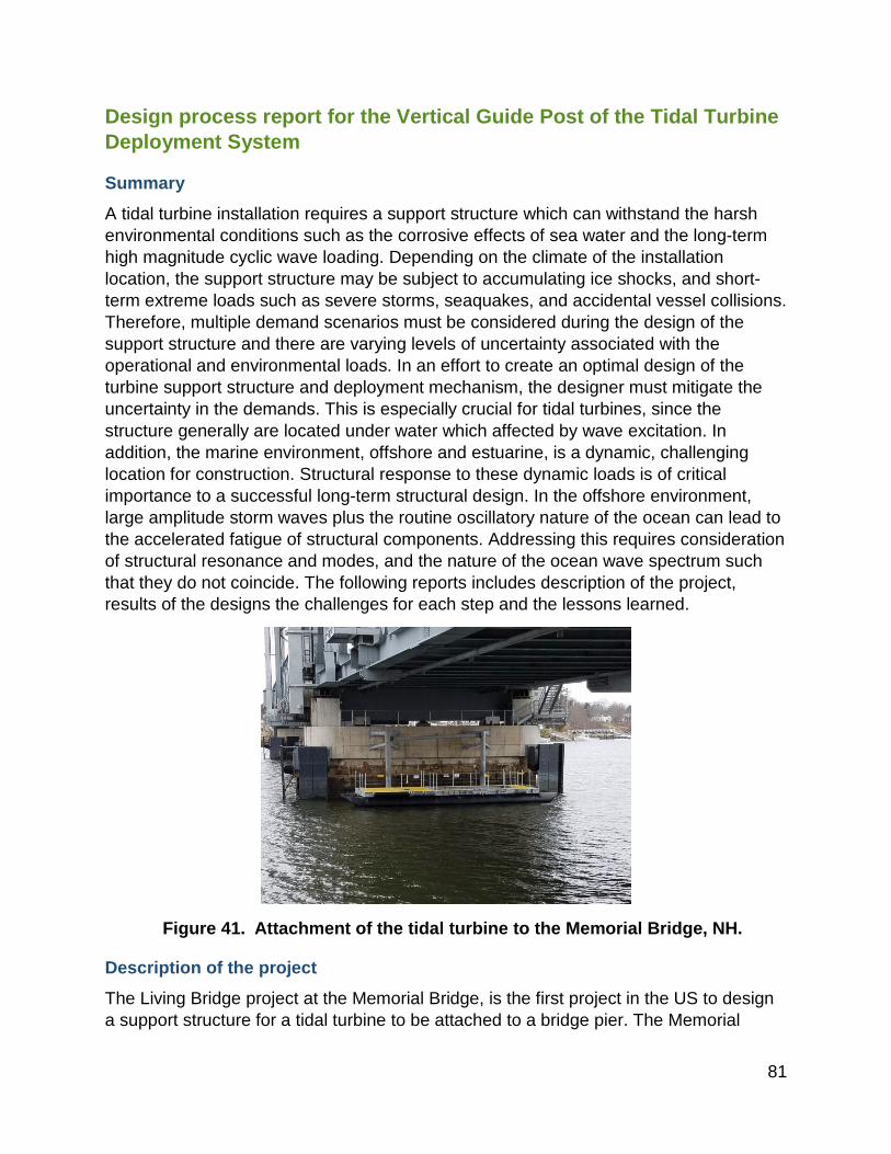
81
Design process report for the Vertical Guide Post of the Tidal Turbine Deployment System
Summary
A tidal turbine installation requires a support structure which can withstand the harsh environmental conditions such as the corrosive effects of sea water and the long-term high magnitude cyclic wave loading. Depending on the climate of the installation location, the support structure may be subject to accumulating ice shocks, and short-term extreme loads such as severe storms, seaquakes, and accidental vessel collisions. Therefore, multiple demand scenarios must be considered during the design of the support structure and there are varying levels of uncertainty associated with the operational and environmental loads. In an effort to create an optimal design of the turbine support structure and deployment mechanism, the designer must mitigate the uncertainty in the demands. This is especially crucial for tidal turbines, since the structure generally are located under water which affected by wave excitation. In addition, the marine environment, offshore and estuarine, is a dynamic, challenging location for construction. Structural response to these dynamic loads is of critical importance to a successful long-term structural design. In the offshore environment, large amplitude storm waves plus the routine oscillatory nature of the ocean can lead to the accelerated fatigue of structural components. Addressing this requires consideration of structural resonance and modes, and the nature of the ocean wave spectrum such that they do not coincide. The following reports includes description of the project, results of the designs the challenges for each step and the lessons learned.
Figure 41. Attachment of the tidal turbine to the Memorial Bridge, NH.
Description of the project
The Living Bridge project at the Memorial Bridge, is the first project in the US to design a support structure for a tidal turbine to be attached to a bridge pier. The Memorial

82
Bridge carries US Route 1 across the Piscataqua River connecting Portsmouth, NH with Kittery, ME. The original Memorial Bridge, constructed in 1923, was a through truss, vertical lift bridge and was replaced with a new gusset-less truss bridge and re-opened in 2013. The Living Bridge Project will transform the Memorial Bridge, into a self-diagnosing, self-reporting, “Smart bridge” powered by a local renewable energy source, tidal energy. The tidal energy conversion system component of this project will convert tidal to electrical energy and serve as a demonstration site of an emerging renewable technology. Therefore, it is aimed to provide a testbed for researchers to study turbine performance and its effects on the bridge and the estuarine environment. The project follows three main goals: structural health monitoring, tidal turbine deployment and performance assessment, and estuarine health monitoring. This report presents the design intelligence created the tidal turbine support structure and a design verification methodology including instrumentation and structural modeling. Installing the tidal turbine support structure directly to the bridge pier is a new concept. A major part of this effort is to provide a calibrated finite element model and analysis procedure to accurately validate both the static and dynamic behavior of the structure and environmental demands. Therefore, a multi-faceted instrumentation and nondestructive testing program is also designed to help for the validation process.
The Tidal Turbine Deployment System (TTDS) as shown in Figure 42 consists of:
a) Vertical guideposts attached to the bridge pier with a 2-meter separation from the face of the pier. The vertical guideposts (VGPs) are made of coated structural steel and have 16” diameter and 0.5” wall thickness. They will be attached to the pier using a four-bolt pattern of one-inch diameter epoxy anchors with twelve inches of embedment.
b) The tidal turbine deployment platform (TTDP) is 15 meters long and 6.67 meters wide. The platform includes a pontoon with 1.06-meter diameter high density polyethylene (HDPE) pontoons and a steel frame which is at the top of the pontoons and defines the platform area. The TTDP has a moon pool to allow for the turbine to rotate through a designed pitching system.

83
Figure 42. Tidal turbine support structure design.
The structural design of the vertical guide posts, tidal turbine deployment platform and anchorage system followed the Allowable Strength Design methodology per the American Institute of Steel Construction’s Manual (14th Edition). The loads used to develop the structural demand were based on the worst-case scenario for expected conditions. Therefore, a three-dimensional structural model of entire support system was created in Sap 2000® to design the structure under the multiple measured loads (shown in Figure 43). The load combinations used were based on the Allowable Stress Design methodology as were the capacity for member design and anchorage.
Figure 43. Three-Dimensional Image (left) and SAP2000® Model (right) of the

84
Numerical Model Description
The support structure includes the A-frame elements, vertical guide posts (VPGs), horizontal members and anchorage. The structure is modeled and analyzed by SAP2000®. As can be viewed in the Figure 43, each VPG is connected to the pier by two skewed A frames which are 3 ft (0.6 m) apart in the vertical direction (z-direction). The A-frame supports provide a 6-ft (1.8 m) separation (in the y-direction) from the VGP and the face of the pier. The support for the A-frames are designed and modeled as fixed ends (constrained in motion and rotation in X, Y and Z direction). All members are designed to have full moment connection on each end, which prevents translation in and rotation around the X, Y, and Z axes.
In order to distribute the demand between the support locations for the two VPGs, the VPGs are connected together by horizontal members at the top and the bottom. The cross-section of the VPGs is designed as a standard 16-inch diameter pipe with a wall thickness of ½-inch. A circular cross section was chosen to enable the pile guides connecting turbine deployment platform (TDP) be moored easily. The VPGs is designed to provide sufficient bending resistance against the horizontal loads applied through turbine, TDP and the structure. In the Table 15, the properties considered in the design of the VGP is expressed for each member.
Table 15. Section properties for the structural steel support structure elements
Structural
Element
Cross section Name
Moment of Inertia, Ix
(cm4)
ASTM Grade
Yield stress, Fy (MPa)
Minimum yield stress,
Fy
Shear modulus
Poisson’s ratio
VGPs HSS16x1/2 HSS10x1/2
28,511 6,618
A500 GrB42
290 42 11154 0.3
A-Frame
HSS8x8x1/2 HSS10x8x1/2
5202 8,907
A500 GrB46
317 46
11154 0.3
Horizontal.
Brace
PIPE8SCH80 W10x19
4.412 4,008
A53GrB A992
241 345
35 50
11154 0.3
In the design, multiple loading conditions is taken into account. However, due to lack of knowledge about performance of the support structures in each category, conservative loads are measured and applied to the model (considering factor of safety 3). The applied loads to the model are as follows:
• Dead load: The dead load considered here is the tidal turbine deployment system (TTDS) itself. The self-weight of the turbine is not included in this analysis.
• Live load: This load is based on considering 250 lb (113.4 kg) for the load of any inspector or maintenance worker. This load is applied concentric to the frame member at the midpoint of the member (Figure 44).
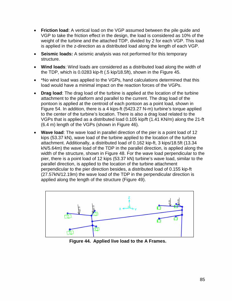
85
• Friction load: A vertical load on the VGP assumed between the pile guide and VGP to take the friction effect in the design, the load is considered as 10% of the weight of the turbine and the attached TDP, divided by 2 for each VGP. This load is applied in the z-direction as a distributed load along the length of each VGP.
• Seismic loads: A seismic analysis was not performed for this temporary structure.
• Wind loads: Wind loads are considered as a distributed load along the width of the TDP, which is 0.0283 kip-ft (.5 kip/18.5ft), shown in the Figure 45.
• *No wind load was applied to the VGPs, hand calculations determined that this load would have a minimal impact on the reaction forces of the VGPs.
• Drag load: The drag load of the turbine is applied at the location of the turbine attachment to the platform and parallel to the current. The drag load of the pontoon is applied at the centroid of each pontoon as a point load, shown in Figure 54. In addition, there is a 4 kips-ft (5423.27 N-m) turbine’s torque applied to the center of the turbine’s location. There is also a drag load related to the VGPs that is applied as a distributed load 0.105 kip/ft (1.41 KN/m) along the 21-ft (6.4 m) length of the VGPs (shown in Figure 46).
• Wave load: The wave load in parallel direction of the pier is a point load of 12 kips (53.37 kN), wave load of the turbine applied to the location of the turbine attachment. Additionally, a distributed load of 0.162 kip-ft, 3 kips/18.5ft (13.34 kN/5.64m) the wave load of the TDP in the parallel direction, is applied along the width of the structure, shown in Figure 48. For the wave load perpendicular to the pier, there is a point load of 12 kips (53.37 kN) turbine’s wave load, similar to the parallel direction, is applied to the location of the turbine attachment perpendicular to the pier direction besides, a distributed load of 0.155 kip-ft (27.57kN/12.19m) the wave load of the TDP in the perpendicular direction is applied along the length of the structure (Figure 49).
Figure 44. Applied live load to the A Frames.
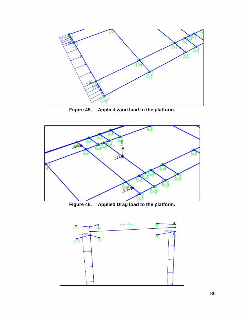
86
Figure 45. Applied wind load to the platform.
Figure 46. Applied Drag load to the platform.
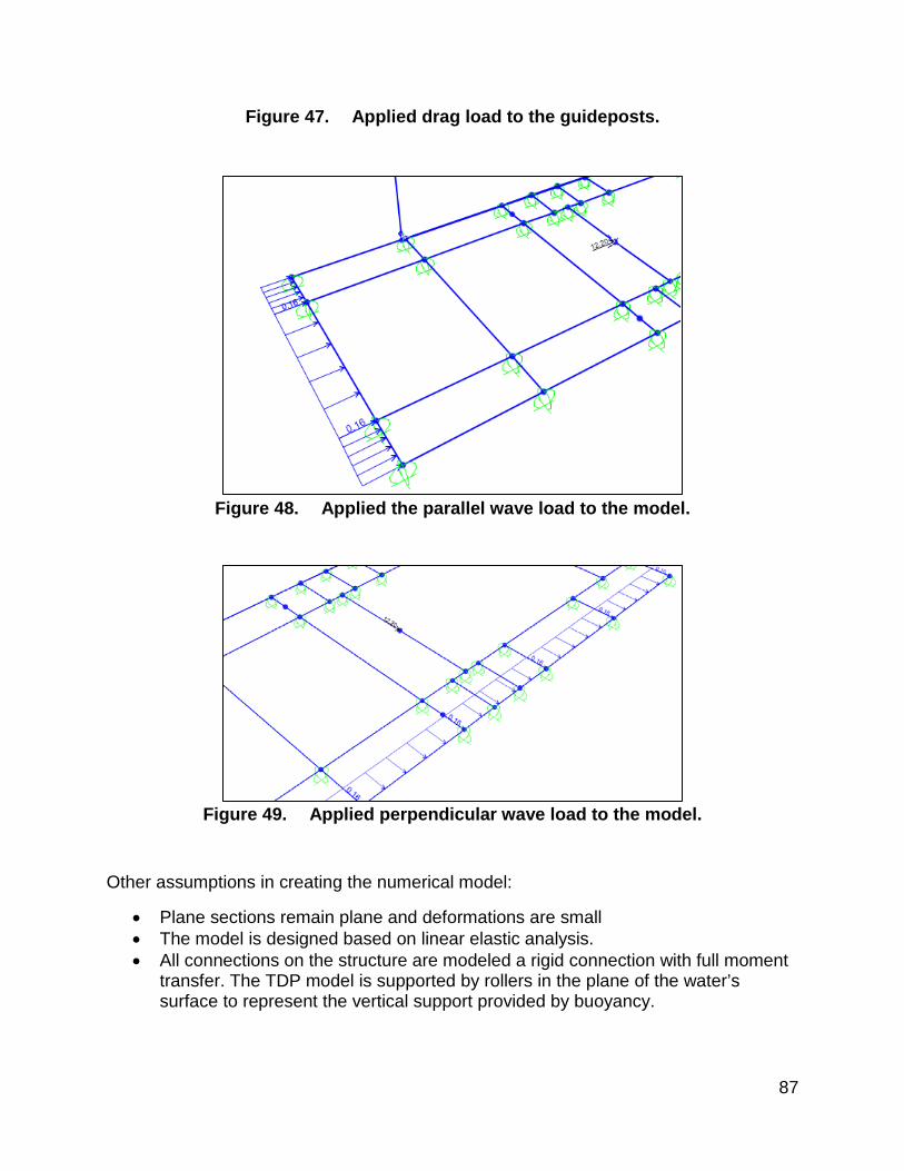
87
Figure 47. Applied drag load to the guideposts.
Figure 48. Applied the parallel wave load to the model.
Figure 49. Applied perpendicular wave load to the model.
Other assumptions in creating the numerical model:
• Plane sections remain plane and deformations are small • The model is designed based on linear elastic analysis. • All connections on the structure are modeled a rigid connection with full moment
transfer. The TDP model is supported by rollers in the plane of the water’s surface to represent the vertical support provided by buoyancy.
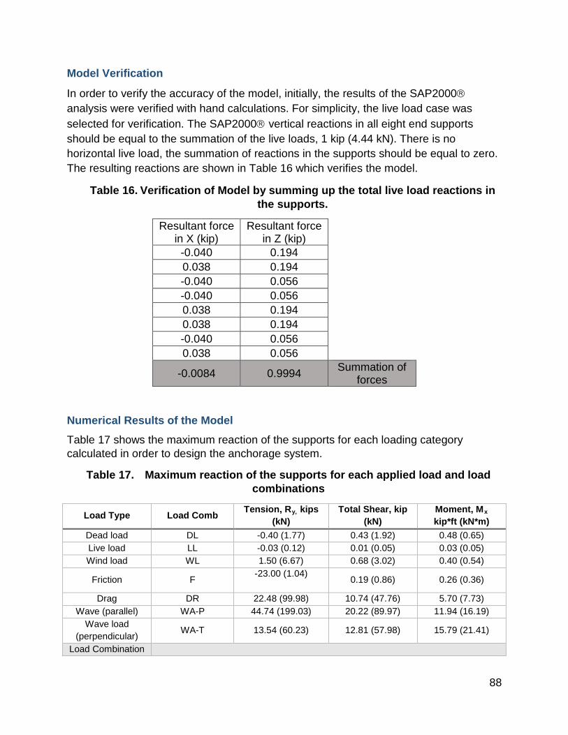
88
Model Verification
In order to verify the accuracy of the model, initially, the results of the SAP2000 analysis were verified with hand calculations. For simplicity, the live load case was selected for verification. The SAP2000 vertical reactions in all eight end supports should be equal to the summation of the live loads, 1 kip (4.44 kN). There is no horizontal live load, the summation of reactions in the supports should be equal to zero. The resulting reactions are shown in Table 16 which verifies the model.
Table 16. Verification of Model by summing up the total live load reactions in the supports.
Resultant force in X (kip)
Resultant force in Z (kip)
-0.040 0.194 0.038 0.194 -0.040 0.056 -0.040 0.056 0.038 0.194 0.038 0.194 -0.040 0.056 0.038 0.056
-0.0084 0.9994 Summation of forces
Numerical Results of the Model
Table 17 shows the maximum reaction of the supports for each loading category calculated in order to design the anchorage system.
Table 17. Maximum reaction of the supports for each applied load and load combinations
Load Type Load Comb Tension, Ry, kips
(kN) Total Shear, kip
(kN) Moment, Mx kip*ft (kN*m)
Dead load DL -0.40 (1.77) 0.43 (1.92) 0.48 (0.65) Live load LL -0.03 (0.12) 0.01 (0.05) 0.03 (0.05) Wind load WL 1.50 (6.67) 0.68 (3.02) 0.40 (0.54)
Friction F -23.00 (1.04)
0.19 (0.86) 0.26 (0.36)
Drag DR 22.48 (99.98) 10.74 (47.76) 5.70 (7.73) Wave (parallel) WA-P 44.74 (199.03) 20.22 (89.97) 11.94 (16.19)
Wave load (perpendicular)
WA-T 13.54 (60.23) 12.81 (57.98) 15.79 (21.41)
Load Combination
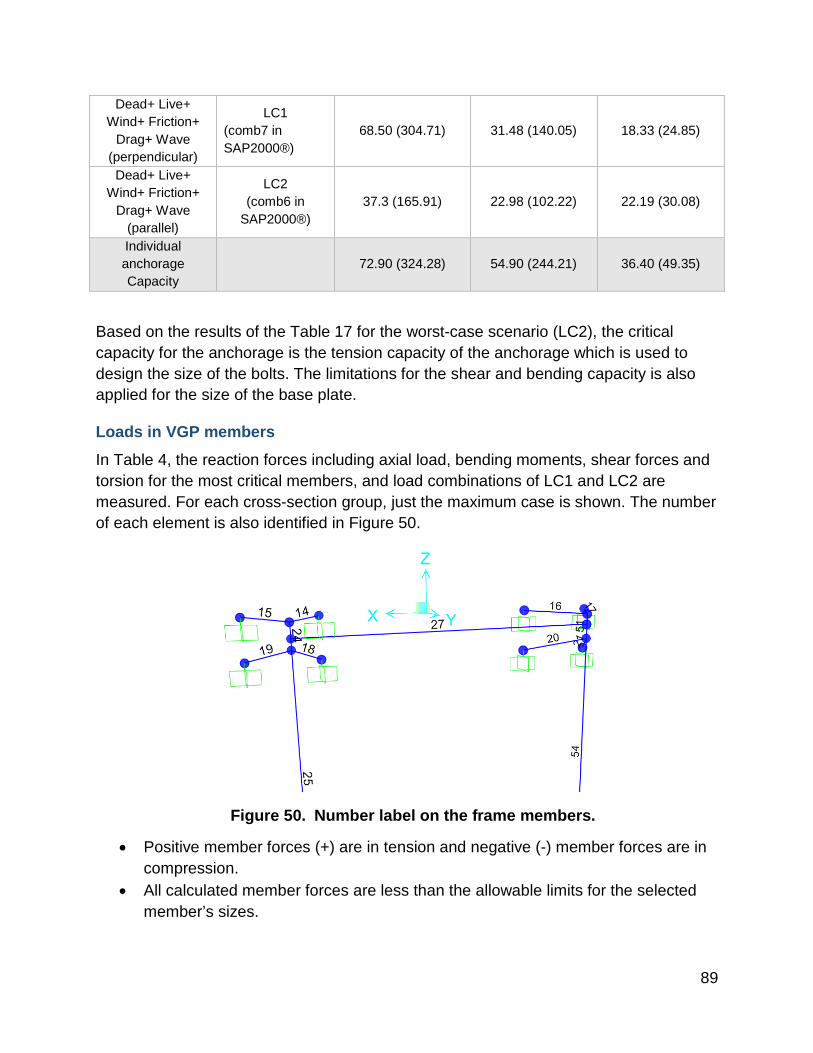
89
Dead+ Live+ Wind+ Friction+
Drag+ Wave (perpendicular)
LC1 (comb7 in SAP2000®)
68.50 (304.71) 31.48 (140.05) 18.33 (24.85)
Dead+ Live+ Wind+ Friction+
Drag+ Wave (parallel)
LC2 (comb6 in
SAP2000®) 37.3 (165.91) 22.98 (102.22) 22.19 (30.08)
Individual anchorage Capacity
72.90 (324.28) 54.90 (244.21) 36.40 (49.35)
Based on the results of the Table 17 for the worst-case scenario (LC2), the critical capacity for the anchorage is the tension capacity of the anchorage which is used to design the size of the bolts. The limitations for the shear and bending capacity is also applied for the size of the base plate.
Loads in VGP members
In Table 4, the reaction forces including axial load, bending moments, shear forces and torsion for the most critical members, and load combinations of LC1 and LC2 are measured. For each cross-section group, just the maximum case is shown. The number of each element is also identified in Figure 50.
Figure 50. Number label on the frame members.
• Positive member forces (+) are in tension and negative (-) member forces are in compression.
• All calculated member forces are less than the allowable limits for the selected member’s sizes.
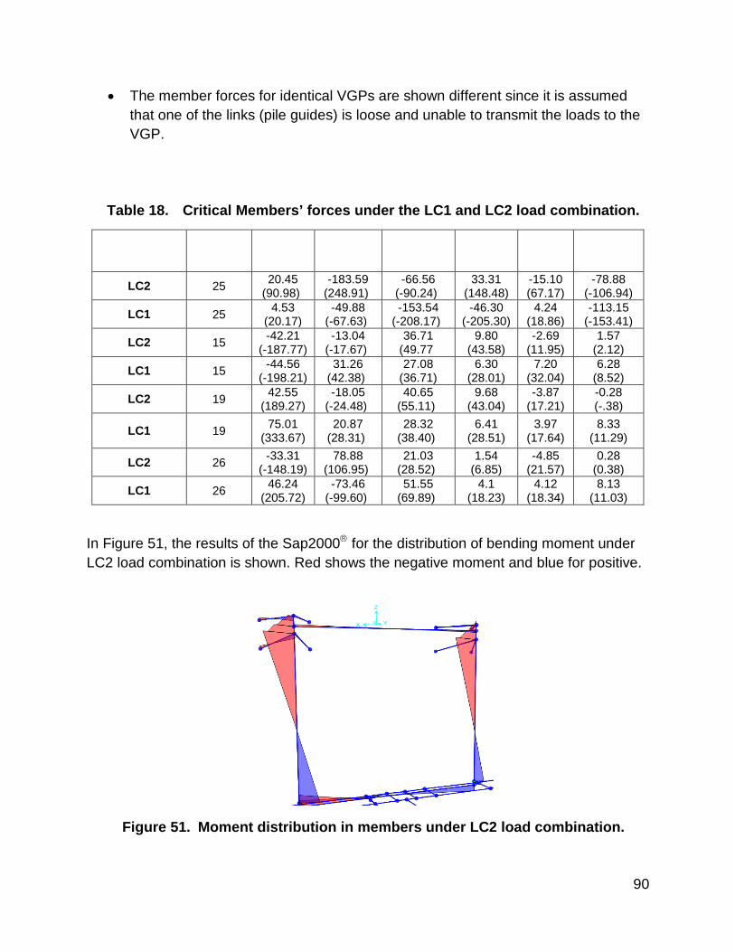
90
• The member forces for identical VGPs are shown different since it is assumed that one of the links (pile guides) is loose and unable to transmit the loads to the VGP.
Table 18. Critical Members’ forces under the LC1 and LC2 load combination.
Load Combination
Frame member
P Kip-ft (KN)
M2-2 Kip-ft
(KN-m)
M3-3 Kips-ft (KN-m)
V2 Kips (KN)
V3 kips (KN)
Torsion kip-ft
(KN-m)
LC2 25 20.45 (90.98))
-183.59 (248.91))
-66.56 (-90.24))
33.31 (148.48)
-15.10 (67.17)
-78.88 (-106.94)
LC1 25 4.53 (20.17)
-49.88 (-67.63))
-153.54 (-208.17))
-46.30 (-205.30)
4.24 (18.86)
-113.15 (-153.41)
LC2 15 -42.21 (-187.77)
-13.04 (-17.67))
36.71 (49.77)
9.80 (43.58)
-2.69 (11.95)
1.57 (2.12)
LC1 15 -44.56 (-198.21)
31.26 (42.38))
27.08 (36.71)
6.30 (28.01)
7.20 (32.04)
6.28 (8.52)
LC2 19 42.55 (189.27)
-18.05 (-24.48))
40.65 (55.11))
9.68 (43.04)
-3.87 (17.21)
-0.28 (-.38)
LC1 19 75.01 (333.67)
20.87 (28.31))
28.32 (38.40))
6.41 (28.51)
3.97 (17.64)
8.33 (11.29)
LC2 26 -33.31 (-148.19)
78.88 (106.95))
21.03 (28.52))
1.54 (6.85)
-4.85 (21.57)
0.28 (0.38)
LC1 26 46.24 (205.72)
-73.46 (-99.60))
51.55 (69.89))
4.1 (18.23)
4.12 (18.34)
8.13 (11.03)
In Figure 51, the results of the Sap2000 for the distribution of bending moment under LC2 load combination is shown. Red shows the negative moment and blue for positive.
Figure 51. Moment distribution in members under LC2 load combination.

91
VGP member capacity calculation
In Table 19, the maximum demand and capacity of the members under the worst load combination, LC2, including axial load, and bending moment over strong and weak axes are shown. The member capacities were calculated using the ASD method. In Table 20, the design ratios are also calculated by dividing each member’s demand by the capacity. The total ratio mentioned in Table 20 is defined by Equation 1 (H1-1b):
The results show that the ratios are low enough to account for a 1/16in section loss around the perimeter of the section for corrosion.
+
+
= (1)
Table 19. Demand and capacity of axial load and bending moments of members.
Member #
Member Location Section Maximum Member Demands Member Capacity
Cross section P
Kips (kN)
M major kip-ft
(kN-m)
M minor kip-ft
(kN-m)
P Kips (kN)
M major kip-ft
(kN-m)
M minor kip-ft
(kN-m)
15 A-frame- Top HSS10x8x0.5 44.55
(198.21) 27.08
(36.72) 31.26
(42.38) 403.22
(1793.65) 119.13
(161.52)
102.15 (138.49)
19 A-frame- Bot HSS 8x8x0.5 42.55
(189.27) 40.65
(55.11) 18.05
(-24.48) 353.92
(1574.32) 86.08
(116.706) 120.55
(163.44)
25 Guide Post HSS 16x0.5 4.50
(20.17) 153.54
(208.17) 49.88
(67.63) 475.83
(2116.65) 222.13
(301.17) 222.13
(301.17)
26 Horizontal Member
Bot
HSS 10x0.5
466.25 (205.72)
47.04 (-63.78)
-73.46 (-99.60)
223.94 (996.14)
88.65 (120.20)
88.65 (120.20)
Table 20. Demand over Capacity ratios for the structural members.
Ratios Member
# Axial ratio
Bending ratio (major)
Bending ratio (minor)
Total ratio Torsion ratio Shear ratio
15 0.06 0.23 0.31 0.59 .04 0.08
19 0.06 0.47 0.21 0.74 0 0.10
25 0.01 0.69 0.23 0.92 -0.35 0.08 26 0.07 0.53 0.83 1.05 .06 0.04
In addition, the SAP2000® analysis recommends using the AISC Equation H3-6, shown in Equations 2, due to high percentage of torsion ratio for the high stressed VGP.

92
≤
+
+
+
+
+
(2)
Vertical Guide Post Anchorage Capacity Design
The anchorage is based on the anchor pattern used for the fenders on the pier. The fender anchorage is comprised of two rectangular patterns of 1 in (0.03 m) anchor rods joined by a 1.5 in (0.04 m) steel plate (Figure 52). The minimum center-to-center distance between anchors in that scheme is 9.2 in (0.23 m). The center-to-center spacing between rows of 18 in (0.46 m) and the anchors have a 12 in (0.3 m) embedment depth. The 1in (0.03) anchor rods are embedded 12 in (0.30m) using Hilti HIT-RE 500-SD mortar or equivalent. Each anchor has allowable capacities of 60.9 kN (13.7 kips) in shear and 80.9 kN (18.2 kips) for pullout. Allowable capacities given by the manufacturer include a safety factor of 4. Combined shear and pullout loading capacity of the anchors is evaluated on a parabolic interaction curve as permitted by ACI 318-11 D.4.1.3. The center-to-center spacing of the anchors on the plate is 12 in (0.30 m) in both directions for this pattern to allow space for connecting members (Figure 60). This is greater than the minimum required per ACI 318-11 D.8.1. Edge distances to the edge of the pier cap face are greater than the minimum of 6*danchor 6 in (0.2 m) required per ACI 318-11 D.8.3.
In order to achieve the necessary overall moment capacity for the structure, four of these rectangular patterns are used to connect each guide post. each four-anchor pattern has its own plate rather than sharing a single large plate with the other four-anchor patterns. The 1 in (0.03 m) thick plate is greater than the 0.88 in (0.022 m) calculated for this size plate bearing on concrete per the AISC Manual Part 14. The capacity of the anchorage system is shown in Table 21.
Figure 52. Anchor plate with four-anchor pattern.

93
Table 21. Capacities of the 4-bolt plate connection.
Four of these plates arranged to connect each guide posts, giving a total of 8 plates and 32 anchors. The pattern is shown in Figure 53. The plates are positioned horizontally such that their centers are 9ft (3m) and 15ft (4.6m) from the centerline of the pier cap face for each guide post. The anchors are positioned vertically on the pile cap such that the top row of anchor bolts lies below the level of the horizontal reinforcement near the top of the pile cap. Detailed calculation of the anchor and the plates are shown in Table 8. Also, Table 23 gives the details for the capacity of the anchor bolts.
Figure 53. Four-plate pattern (connection for one guide post).
Type of Loading Capacity Pullout 72.9 kip (324 kN) Shear 54.9 kip (244 kN) Horizontal Plane Moment 36.5 kip*ft (49.5 kN*m) Vertical Plane Moment 36.5 kip*ft (49.5 kN*m) Connection Plane Moment 38.8 kip*ft (52.6 kN*m)

94
Table 22. Calculations for anchor plate minimum thickness.
Item Value Equation Reference
Concrete Strength f'c 4000 psi
Required Strength Pa 73000 lbs
Plate Steel Strength Fy 36000 psi
Compression Member Dimensions d 8 in
b 8 in Plate Overall Dimensions N 20 in
B 20 in Plate Cantilever Dimensions m 6.2 in =(N-0.95*d)/2 [AISC Eq. 14-2]
n 6.8 in =(B-0.8*bf)/2 [AISC Eq. 14-3]
n 2 in =(d*bf)0.5/4 [AISC Eq. 14-4]
» 1 (conservative) [AISC Eq. 14-5]
»n 2 in =»*n'
Critical Cantilever Dimension l 6.8 =max(m,n,»n') [AISC p. 14-6] Minimum Plate Thickness tmin 0.88 in =l*(3.33*Pa/(Fy*B*N))0.5 [AISC Eq. 14-7b]
Table 23. The details for the capacity of the anchor bolts
Item Value Calc/Reference Allowable Anchor Pullout Capacity Na 18.2
3 kip Hilti Product Technical Guide (ASD
values) Allowable Anchor Shear Capacity Va 13.7
3 kip Hilti Product Technical Guide (ASD
values) Anchor Vertical Spacing m 12.0
0 in (minimum is 6*d = 6" per ACI 318-11
D.8.3) Anchor Horizontal Spacing n 12.0
0 in (minimum is 6*d = 6" per ACI 318-11
D.8.3) Anchor Radial Distance from Center of Plate
r 8.49 in
Anchor Plate Allowable Pullout Na,plat
e 72.9 in =4 anchors * Na
Anchor Plate Allowable Shear Va,plate 54.9 in =4 anchors * Va Anchor Plate Allowable Moment (Vertical Plane)
Ma,vert 36.5 kip-ft =2 anchors * Na* m * (1'/12")
Anchor Plate Allowable Moment (Horizontal Plane)
Ma,horz 36.5 kip-ft =2 anchors * Na* n* (1'/12")
Anchor Plate Allowable Moment (Connection Plane)
Ta 38.8 kip-ft =4 anchors * Va* r * (1'/12")
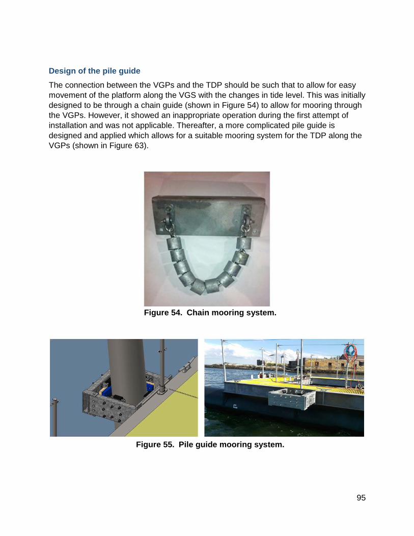
95
Design of the pile guide
The connection between the VGPs and the TDP should be such that to allow for easy movement of the platform along the VGS with the changes in tide level. This was initially designed to be through a chain guide (shown in Figure 54) to allow for mooring through the VGPs. However, it showed an inappropriate operation during the first attempt of installation and was not applicable. Thereafter, a more complicated pile guide is designed and applied which allows for a suitable mooring system for the TDP along the VGPs (shown in Figure 63).
Figure 54. Chain mooring system.
Figure 55. Pile guide mooring system.
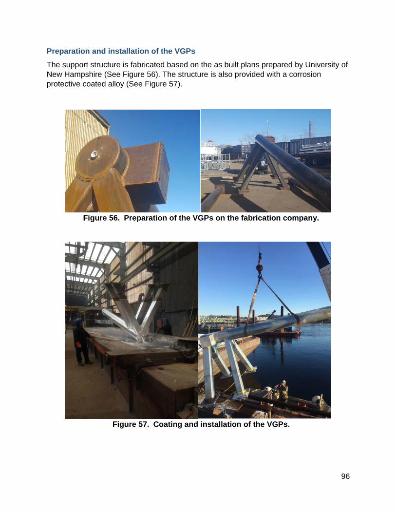
96
Preparation and installation of the VGPs
The support structure is fabricated based on the as built plans prepared by University of New Hampshire (See Figure 56). The structure is also provided with a corrosion protective coated alloy (See Figure 57).
Figure 56. Preparation of the VGPs on the fabrication company.
Figure 57. Coating and installation of the VGPs.

97
Monitoring system of VGPs
Due to the uncertain behavior of dynamic loads, wave and wind load which threaten the support structure as well as the Memorial Bridge’s pier, a long-term monitoring program for the support structure is defined. The monitoring program includes the strain gauges which are permanently installed at multiple location of the vertical guide posts. The instrumentation plan is designed based on the high stressed areas which identified in the design of the structure by the software as well as the accessibility of the location. The instrumentation plan is shown in Figure 58. Data collection for the health monitoring program of the vertical guideposts started since late October 2017. The long-term collected data aims to verify the design assumption as well as to investigate the influence of the seasonal changes on the structures. In addition, through the comparison between the data before and after turbine installation, the influence of turbine’s operation on the structures can be followed. In the Figure 59 a sample of the collected data of strain gauges for a single day (24 hours) is shown. As shown in the graph, the structure can have reasonable amount of strain due to the high values of dynamic loads which is required to be monitored regularly. As-built plan for the vertical guide posts is depicted in Figure 60.
Figure 58. Instrumentation plan for vertical guide posts.
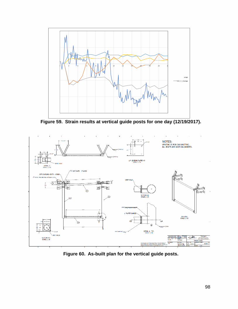
98
Figure 59. Strain results at vertical guide posts for one day (12/19/2017).
Figure 60. As-built plan for the vertical guide posts.
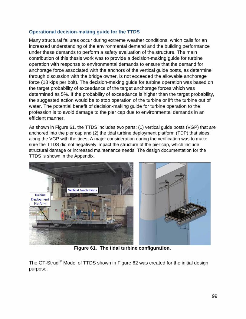
99
Operational decision-making guide for the TTDS
Many structural failures occur during extreme weather conditions, which calls for an increased understanding of the environmental demand and the building performance under these demands to perform a safety evaluation of the structure. The main contribution of this thesis work was to provide a decision-making guide for turbine operation with response to environmental demands to ensure that the demand for anchorage force associated with the anchors of the vertical guide posts, as determine through discussion with the bridge owner, is not exceeded the allowable anchorage force (18 kips per bolt). The decision-making guide for turbine operation was based on the target probability of exceedance of the target anchorage forces which was determined as 5%. If the probability of exceedance is higher than the target probability, the suggested action would be to stop operation of the turbine or lift the turbine out of water. The potential benefit of decision-making guide for turbine operation to the profession is to avoid damage to the pier cap due to environmental demands in an efficient manner.
As shown in Figure 61, the TTDS includes two parts; (1) vertical guide posts (VGP) that are anchored into the pier cap and (2) the tidal turbine deployment platform (TDP) that sides along the VGP with the tides. A major consideration during the verification was to make sure the TTDS did not negatively impact the structure of the pier cap, which include structural damage or increased maintenance needs. The design documentation for the TTDS is shown in the Appendix.
Figure 61. The tidal turbine configuration.
The GT-Strudl® Model of TTDS shown in Figure 62 was created for the initial design purpose.

100
Figure 62. Gt-Strudl® model of the tidal turbine deployment system.
The initial design of the TTDS (Tidal Turbine Deployment System) was based upon the expected ‘worst events’ due to the uncertainties associated with the wave loads, drag loads, wind speeds magnitudes and limitations of the design codes application to this structure. Design loads that were considered in this study are shown in Table 24.
Table 24. Design load cases of the tidal turbine deployment system.
Load demands were developed with input from faculty and students from the ocean engineering program at UNH. These demands include the dead load of the turbine, wind load, wave load, and the drag loads. Analytical investigations were performed for different load case scenarios applied to the TTDS:
• 30 different wave heights (from 0.1 ft to 3 ft, step interval 0.1) • 10 different wind speeds (from 10 mph to 100 mph, step interval 10)

101
• 3 different drafts (deep draft with turbine on/off and shallow draft) • 2 different wave directions (parallel and perpendicular waves) • 18 different wavelengths:
o Perpendicular waves: from 30.3 ft to 100 ft o Parallel waves: from 75.9 ft to 130 ft
The load cases took into account that there were many different load conditions due to the variability of the wind speeds, the wave heights, the wavelengths, directions of waves, and the floating drafts (deep draft and shallow draft). Each load case generated structural conditions that were used to determine the turbine’s position and operating condition: lifting the tidal turbine out of water or just shutting the turbine down. Each load case was analyzed using GT-Strudl® models. The results of each analytical run were used to develop a more accurate idea of the effects on the anchorage due to the different load cases. As the two main uncertainties were wave load and wind load. The probability calculation of the anchorage forces was based on different wave height, wind speed, and wavelength. With the probability of exceedance being greater than 5%, a decision needs to be made to either shut down turbine or lift it out of water. Table 25 and Table 26 summarize overall Probability of Calculations (POE) with varied wind speed and wave height. According to the results, it was concluded that: a) turbine shall be shut down when the wind speed is higher than 80 mph, b) turbine shall be shut down when the wave height is higher than 2.8 ft with wavelength range of the parallel wave load from 75.9 ft to 140 ft, c) The platform shall be removed when the deployment system is subject to extreme conditions (e.g. superstorms).
Table 25. Overall POE calculations with varied wind speed.
Table 26. Overall POE calculations with varied wave height.

102
Challenges
• The calculated dynamic loads, wave, wind and drag loads are measure for the worst-case scenario which the structure in unlikely to experience. This is due to lack of any p\experience on the design of this un-parallel structure and the restricted knowledge on the environmental loading condition of the area.
• The limited b capacity for the anchorage system and the concerns of the bridge’s owner to minimize the damage to the prier through the anchors, puts another restriction for the design. Therefore, the design should be such that the total produced reaction loads at the supports be less the capacity of the anchors.
• Unknown capacity of the concrete material of the pier. Generally, for determining the actual material properties of the current structures some destructive testing may be applied. However, due to lack of such results, the material properties are assumed on based on the available information. In expense, a reasonable level for factor of safety is taken into account.
• The worst-case loading combinations defined for the design may be considered conservative. However, this is due to lack of any recommendations in the current steel codes for this type of structures.
• The designer has to do a deep review on the past experienced hazards experienced by off-shore structure to consider similar in the design. For instance, for the current design, it is assumed that if one of the pile guides becomes loos, the other should be capable enough to carry the TDP.
• The software SAP 2000® does not consider the dynamic behavior of the wave and wind loads. Also, it doesn’t consider the buoyancy behavior of the water. In addition, the dynamic behavior of the turbine under water may add extra load to the structure which is unlikely to measure.
• Another challenge was the concerns for the pile guide performance. If for some reason the pile guide gets stuck, the platform will face with movement problem.
Lessons learned
• The innovative design of the vertical guide posts provides the opportunity to the designer(student) to have the courage to design a different and un parallel structures which never did during the education. The student will apply the materials learned in steel design for a different application.
• Design of a structure under dynamic loads with high variability (wind and wave) requires getting enough knowledge about the calculation and application of the loads, the risks. It also requires to be familiarized with the environmental conditions of the area (flood, ice, tide level, wind and wave speed, …).

103
• Long-term monitoring of this structure provides the opportunity to verify the design assumptions and improve the design for further applications. It also enables us to study environmental effects on the structure for long-term condition assessment.

104
References • Adams, T., Mashayekhizadeh, M., Santini-Bell, E., Wosnik, M., Baldwin, K., Fu, T.
(2017) “Structural Response Monitoring of a Vertical Lift Truss Bridge”, 96th Transportation Research Board Annual Meeting Compendium of Papers, Washington D.C, January 8-12, 17-06353.
• AASHTO. (2012). “AASHTO LRFD Bridge Design Specifications. American Association of State Highway and Transportation Officials,” Washington, D.C.
• Downing S.D., Socie D.F. (1982). “Simple rainflow counting algorithms,” International Journal of Fatigue 4 (1), 31-40.
• FHWA. (2015). “Compilation of Existing State Truck Size and Weight Limit Laws,” Report to Congress. Washington, D.C.
• Fricke, W. (2001) “Recommended Hot Spot Analysis Procedure for Structural Details of FPSOs And Ships Based on Round-Robin FE Analyses,” The Eleventh International Offshore and Polar Engineering Conference. Stavanger, Norway.
• Fischer, F. (2018). “Design and Fabrication of a Specimen and Experimental Setup for Fatigue Testing of a Gusset-less Bridge Connection.” M.Sc. thesis, University of New Hampshire, NH, USA.
• Manning, T. E. (2017). “Enhanced in-service condition assessment of bridges using GoPro® cameras,” M. Sc. Thesis, University of New Hampshire.
• Mashayekhizadeh, M., Adams,T., Yang,C., Gagnon,I., Wosnik,M., Baldwin, K., Santini-Bell, E. (2016) ”Structural Health Monitoring and Design Verification of Tidal Turbine Support Structure”, Proceedings of 75th ASNT Annual Conference, Long Beach, CA.
• Mashayekhizadeh, M., Santini-Bell, E. and Adams, T. (2017). “Instrumentation and Structural Health Monitoring of a Vertical Lift Bridge”, Proceedings of the 26th ASNT Research Symposium, Jacksonville, FL.
• Santini-Bell, E., Mashayekhizadeh, M., Adams, T., Nash, T. (2017) “Structural Monitoring to Support Decision-Making on the A Vertical Lift Bridge”, Proceedings of the Twelfth International Conference on Structural Safety and Reliability (ICOSSAR), Vienna, 2386-2395.
• Mashayekhizadeh, M., Santini-Bell, E. (2018) “Influence of temperature in vibration-based structural health monitoring of a vertical lift bridge”, 27th ASNT Research Symposium, Orlando, FL.
• Mashayekhizadeh, M., Mehrkash, M., Shahsavari, V., and Santini-Bell, E. (2018). “Multi-scale finite element model development for long-term condition assessment of vertical lift bridge,” ASCE Structures Congress, Fort Worth, TX.
• Mashayekhizadeh, M., Bell, E. (2018) “Data Validated Multi-Scale Finite Element Modeling Protocol for Complex Connections of a Movable Bridge”, Engineering Mechanics Institute Conference, Cambridge, MA.

105
• Mashayekhi, M. and Santini-Bell, E.* (2018). “Developing three-dimensional multi-scale finite element model for in-plane service performance assessment of bridges” Computer-Aided Civil and Infrastructure Engineering, 34(5), 385-403.
• Mashayekhi, M., Santini-Bell, E. (2019) “Including Environmental and Vertical Lift Excitations for Structural Condition Assessment of a Gusset-less Truss Bridge”, 28th ASNT Research Symposium, Garden Grove, CA.
• Mashayekhi, M., Santini-Bell, E. (2019a) “Fatigue assessment of the gusset-less connection using field data and numerical model” 10th New York City Bridge Conference, New York.
• Mashayekhi, M., Santini-Bell, E. (2019b) “Detection of damage-induced fatigue response based on structural health monitoring data of in-service steel bridges using Artificial Neural Network” 12th International Workshop on Structural Health Monitoring, IWSHM, Stanford, CA.
• McGeehan, D., Zargar Shoushtari, S., Medina, R. and Santini-Bell, E. (2019). “Comparison of multiple strain measurement techniques to characterize the behavior of an experimental fatigue test.” 98th Annual Meeting of Transportation Research Board, Washington D.C.
• McGeehan, D. W. (2018). “Experimental Evaluation of Fatigue Test Setup for a Gusset-less Truss Connection.” M.Sc. thesis, University of New Hampshire, NH, USA.
• Mehrkash, M., and Santini-Bell, E. (2018a). “Modeling and characterization of complicated connections in structural and mechanical systems as applied to a gusset-less truss connection,” 97th Annual Meeting of Transportation Research Board, Washington D.C.
• Mehrkash, M., Shahsavari, M., and Santini-Bell, E. (2018). “Instrumentation sufficiency of a vertical lift bridge for modal system identification by frequency domain analysis,” Engineering Mechanics Institute Conference, Cambridge, MA.
• Mehrkash, M., and Santini-Bell, E. (2018b). “System identification of a bridge gusset-less connection by simplified and detailed local analytical models,” NDE/NDT for Highway and Bridges: Structural Materials Technology and the International Symposium on Non-Destructive Testing in Civil Engineering, New Brunswick, NJ.
• Mehrkash, M., and Santini-Bell, E. (2019a). “Finite element model updating of the UCF Grid benchmark connections using experimental modal data,” 37th International Modal Analysis Conference, Orlando, FL.
• Mehrkash, M., Shahsavari, V., and Santini-Bell, E. (2019). “Instrumentation plan verification for damage detection of a vertical lift steel truss bridge,” SPIE Smart Structures and Nondestructive Evaluation, Denver, CO.
• Mehrkash, M., and Santini-Bell, E. (2019b). “Local condition assessment and damage detection of gusset-less connections used in a vertical lift truss bridge,” 9th International Conference on Structural Health Monitoring of Intelligent Infrastructure, St. Louis, MO.

106
• Miner, M.A. (1945).” Cumulative Damage in Fatigue,” Journal of Applied Mechanics, 67, A159.
• Nash, T. P. (2016). “An objective protocol for movable bridge operation in high-wind events based on hybrid analyses by European and American design code,” M. Sc. Thesis, University of New Hampshire.
• Nash, T., Santini-Bell, E., Mehrkash, M., and Shahsavari, V. (2018), “An objective decision-making protocol for lift bridge operation subjected to high wind loads,” Engineering Mechanics Institute Conference, Cambridge, MA.
• Niemi, E., Tanskanen, P. (1999). “Hot Spot Stress Determination for Welded Edge Gussets,” The International Institute of Welding - IIW Doc. XIII-1781-99.
• Niemi, E., Fricke, W., Maddox, S.J. (2016). “Structural Hot-Spot Stress Approach to Fatigue Analysis of Welded Components, XIII-2636r3-16 XV-1521r3-16. Designer’s Guide”, International Institute of welding (2), Singapore, Singapore, Springer.
• Radaj, D. (1990) “Design and analysis of fatigue resistant welded structures,” Cambridge, UK: Abington Publishing.
• Shahsavari, V., Mehrkash, M., and Santini-Bell, E. (2018a). “Structural health monitoring of a vertical lift bridge using vibration data,” 27th ASNT Research Symposium, Orlando, FL.
• Shahsavari, V., Mehrkash, M., and Santini-Bell, E. (2018b). “Effect of damaged structural members on performance degradation of a vertical lift truss bridge,” ASNT Annual Conference, Houston, TX.
• Shahsavari, V., Mehrkash, M., and Santini-Bell, E. (2019). Progressive damage assessment and vulnerability evaluation of a vertical lift steel gusset-less truss bridge by wavelet analysis, 28th ASNT Research Symposium, Garden Grove, CA.
• Yang, C., Santini-Bell, E., Shahsavari, V., and Mehrkash, M. (2018). “Probability-based demand evaluation of the bridge tidal turbine deployment system subject to environmental events, Engineering Mechanics Institute Conference,” Cambridge, MA.