This content has been downloaded from IOPscience. Please scroll down to see the full text.

Download details:

IP Address: 169.230.243.252

This content was downloaded on 06/09/2014 at 13:53

Please note that terms and conditions apply.

Accelerating and retarding anomalous diffusion

View the table of contents for this issue, or go to the journal homepage for more

2012 J. Phys. A: Math. Theor. 45 145001

(http://iopscience.iop.org/1751-8121/45/14/145001)

Home Search Collections Journals About Contact us My IOPscience

IOP PUBLISHING JOURNAL OF PHYSICS A: MATHEMATICAL AND THEORETICAL

J. Phys. A: Math. Theor. 45 (2012) 145001 (17pp) doi:10.1088/1751-8113/45/14/145001

Accelerating and retarding anomalous diffusion

Chai Hok Eab1 and S C Lim2

1 Department of Chemistry Faculty of Science, Chulalongkorn University, Bangkok 10330,Thailand2 Faculty of Engineering, Multimedia University, 63100 Cyberjaya, Selangor Darul Ehsan,Malaysia

E-mail: Chaihok.E@chula.ac.th and sclim47@gmail.com

Received 27 January 2012, in final form 27 February 2012Published 23 March 2012Online at stacks.iop.org/JPhysA/45/145001

AbstractIn this paper, Gaussian models of retarded and accelerated anomalous diffusionare considered. Stochastic differential equations of fractional order driven bysingle or multiple fractional Gaussian noise terms are introduced to describeretarding and accelerating subdiffusion and superdiffusion. Short- and long-time asymptotic limits of the mean-squared displacement of the stochasticprocesses associated with the solutions of these equations are studied. Specificcases of these equations are shown to provide possible descriptions of retardingor accelerating anomalous diffusion.

PACS numbers: 02.50.Ey, 05.40.−a

(Some figures may appear in colour only in the online journal)

1. Introduction

Anomalous diffusion occurs in many physical, chemical and biological systems [1–3]. Innormal diffusion, the mean-squared displacement of diffusion particles varies linearly withtime 〈�x2(t)〉 ∼ t. In some complex disordered media, the diffusion becomes anomalous with〈�x2(t)〉 ∼ tα , where the scaling exponent α �= 1 characterizes the anomalous diffusion. Forα < 1, the process is known as subdiffusion, and when α > 1 it is called superdiffusion.The fractal dimension of the trajectory of anomalous diffusion was studied in 1982 [4], whichcan be considered the first attempt to link fractional derivative with anomalous diffusion.It is widely accepted now that differential equations of fractional order are well suited fordescribing fractal phenomena such as anomalous diffusion in complex disordered media. Theconstant memory and self-similar character of these phenomena can be taken into account byusing the kinetic equations with fixed fractional order.

In certain locally heterogeneous media, diffusing processes do not satisfy the constantpower-law-type scaling behavior like anomalous diffusion. Such processes include the

1751-8113/12/145001+17$33.00 © 2012 IOP Publishing Ltd Printed in the UK & the USA 1

J. Phys. A: Math. Theor. 45 (2012) 145001 C H Eab and S C Lim

retarding and accelerating anomalous diffusion. Retardation of diffusion occurs in single-file diffusion, where particles are constrained to move in a single file due to confined one-dimensional geometry, such as diffusion in zeolites [5], or in the anomalous diffusion thatoccurs on the biological cell membrane [6, 7]. Possible causes for the presence of anomaloussubdiffusion in biological systems include the presence of immobilized obstacles whichhamper molecular motion by an excluded volume interaction and the cytoplasmic crowding inliving cells. On the other hand, membrane-bound proteins exhibit transition from subdiffusionat short time to normal or superdiffusion at long times [8]; the diffusion of telomeres in thenucleus of mammalian cells shows accelerating subdiffusion [9]. Other examples are retardedand enhanced dopant diffusion in semiconductors [10–12], the accelerating superdiffusion ofenergetic charged particles across the magnetic field in astrophysical plasma physics [13, 14]and accelerated diffusion in the Josephson junction [15]. Such processes have memory andfractal dimension that may vary with position, temperature, density, or internal parameterssuch as elasticity and viscosity.

Anomalous diffusion having a scaling exponent which varies with position and time wasstudied by Glimm and co-workers in the early 1990s [16, 17] in the multifractal modelingof heterogeneous geological systems. More systematic studies of transport phenomenawith variable scaling exponents were carried out in the late 1990s and early 2000s.Stochastic processes with variable fractional order such as multifractional Brownian motionwas introduced to model phenomena with variable memory or variable fractal dimension[18–20]. In order to describe systems with variable scaling exponents, one may have toconsider fractional differential equations of variable order. However, such variable orderequations are in general mathematically intractable and cannot be solved without numericalapproximations [21–26].

There exists a certain class of diffusion processes with a non-unique scaling exponentthat can be described by fractional differential equations of distributed order. The notionof distributed-order differential operators was first introduced by Caputo in 1969 [27]. Adistributed-order fractional diffusion equation has its fractional order derivatives integratedover the order of differentiation within a given range. Applications of distributed fractionalorder equations to fractional diffusion and fractional relaxation have been carried out byvarious authors [25–33].

This paper considers Gaussian models of retarded and accelerated anomalous diffusion.We introduce a class of multi-term fractional Langevin-type equations driven by single ormultiple fractional Gaussian noise terms. These equations can be regarded as special cases offractional Langevin equations of distributed order, and they can be used to describe retardedand accelerated anomalous diffusion. Detailed study of the short- and long-time asymptoticproperties of the solutions to these equations is carried out.

2. Multi-fractional stochastic differential equations

In this section, we introduce a class of multi-fractional Langevin-like equations of the followingform:

m∑i=1

aiDαi x(t) =

n∑j=1

c jξγ j , t ∈ R, 0 < αi � 2, (1)

2

J. Phys. A: Math. Theor. 45 (2012) 145001 C H Eab and S C Lim

where c j > 0, Dαit is the Riemann–Liouville or Caputo fractional derivative [34–38] which is

defined for m − 1 � α � m as

Dαt f (t) =

⎧⎪⎪⎨⎪⎪⎩1

�(m − α)

dm

dtm

∫ t

0

f (u) du

(t − u)α−m+1, Riemann−Liouville

1

�(m − α)

∫ t

0(t − u)m−α−1 dm

dtmf (u) du, Caputo.

(2)

The Gaussian noise ξγ j (t) is defined by

〈ξγ j (t)〉 = 0, (3)

and

〈ξγi (t)ξγ j (s)〉 = δi jd j|t − s|−γ j , 0 < γi, γ j < 2, (4)

with

dj = 1

2 sin(πγ j/2)�(1 − γ j). (5)

If we let γ j = 2 − 2Hj, where 0 < Hj < 1 is the Hurst index associated with fractionalBrownian motion, and d j = (2 sin(πHj)�(2Hj − 1))−1, then ξγ j (t) can be regarded as thederivative (in the sense of generalized functions) of the fractional Brownian motion indexedby Hj. Note that the covariance of fractional Gaussian noise has the same algebraic sign as(2Hj − 1). For 1/2 � Hj < 1, the process exhibits long-range dependence with persistentpositive covariance. On the other hand, when 0 < Hj < 1/2, d j is negative and the processhas an anti-persistent correlation structure. For Hj = 1/2, or γ j = 1, it corresponds to whitenoise. Here, we remark that limHj→1/2 d j|t|2Hj−2 = δ(t) in the sense of generalized functions[39, 40]. We thus see that there is no need to include in the covariance of fractional Gaussiannoise ξ (t) an extra term to cater for the white noise when H = 1/2 as given by [41]

〈ξHj (t)ξHj (s)〉 = 4d jHj(2Hj − 1)|t − s|2Hj−2 + 4d jHj|t − s|2Hj−1δ(t − s). (6)

Here, we would like to briefly discuss the covariance of fractional Gaussian noise [41–43] interms of generalized functions. Just like for a proper description of fractional Gaussian noise,ξ (t) should not be defined pointwise for each t. Instead, the process needs to be consideredas a linear functional in some test function space such as Schwarz space S (R) of real-valuedinfinitely differentiable functions which decrease rapidly [39]. The generalized process ξ (t),f ∈ S (R), is a linear functional

ξ ( f ) =∫ ∞

−∞ξ (t) f (t) dt. (7)

ξ ( f ) is a generalized stationary Gaussian process with the covariance given by the bilinearfunctional

C( f , g) = 〈ξ ( f )ξ (g)〉 =∫ ∞

−∞

∫ ∞

−∞f (t)g(s)c(t − s) dt ds

=∫ ∞

−∞f (t) dt

∫ ∞

−∞g(s)c(|t − s|) ds

=∫ ∞

−∞f (t) dt

∫ ∞

0c(s)[g(t + s) + g(t − s)] ds, (8)

where c(t − s) is a generalized function or distribution. For example, for H = 1/2, ξ is whitenoise with c(t − s) = δ(t − s). H �= 1/2 corresponds to fractional Gaussian noise, with c(t),t > 0, given by

c(t) = t2H−2

sin(πH)�(2H − 1)=

⎧⎪⎨⎪⎩1

sin(πH)I2H−1δ(t), 1/2 < H < 1

1

sin(πH)D1−2Hδ(t), 0 < H < 1/2.

(9)

3

J. Phys. A: Math. Theor. 45 (2012) 145001 C H Eab and S C Lim

When 1/2 < H < 1, the covariance kernel in (8) can be regarded as the fractional integralof the delta function, I2H−1δ(t), up to a multiplicative constant (2 sin(πH))−1. In this case,c(t − s) is locally integrable. It becomes the fractional derivative of the delta function for(2 sin(πH))−1D1−2Hδ(t) for 0 < H < 1/2 since Iα f = D−α f [43].

Before we proceed further, a brief comment on the stochastic differential equation drivenby fractional Gaussian noise will be given. Recall that stochastic calculus of Ito cannot beused to define the integrals with respect to a stochastic process which is not a semimartingale.Fractional Brownian motion (except for the case of Brownian motion case with H = 1/2)is not a semimartingale. Due to its widespread application, the question on how to obtaina well-defined stochastic integral with respect to fractional Brownian motion has become along standing problem which has attracted considerable attention [44, 45]. Several methodswhich include Sokorohod–Stratonovich stochastic integrals, Malliavin calculus and pathwisestochastic calculus have been proposed to overcome this difficulty (see [45, 46] for details).However, for application purposes, theory based on abstract integrals may encounter difficultyin physical interpretations. As we shall restrict our discussion related to applications offractional Gaussian noise involving only persistent case 1/2 < Hj < 1 (or 0 < γ j < 1),the integrals with respect to the fractional Brownian motion can thus be treated as the pathwiseRiemann–Stieltjes integrals (see for example [46] and references given there). This allows oneto handle such integrals in a similar way as ordinary integrals.

Here, we remark that the multi-term fractional-order Langevin-like equation (1) can alsobe regarded as a special class of the following distributed-order fractional time stochasticequation:

Dϕx(t) = ξψ (t), t � 0, (10)

with the distributed fractional derivative

Dϕx(t) =∫ 2

0ϕ(α)Dα

t x(t) dα, (11)

where Dαt is the fractional derivative as defined by (2), the weight function ϕ(α), 0 � α � 2,

which satisfies ϕ(α) � 0 is given by ϕ(α) = ∑mi=1 aiδ(α−αi). Note that in general the weight

function is a positive generalized function. The Gaussian noise ξψ (t) is the distributed-orderfractional Gaussian noise defined by

ξψ (t) =∫ 2

0ξγ (t)ψ(γ ) dγ , (12)

with the weight function ψ(γ ), 0 � γ � 2, which satisfies ψ(γ ) � 0 and is given byψ(γ ) = ∑n

j=1 c jδ(γ − γ j). Here, we remark that in most of the examples consideredsubsequently, we shall restrict 0 � γ � 1.

The solution of (1) can be solved formally by using the Laplace transform method whichgives

A(p)x(p) − B(p) = ξ (p), (13)

where x(p) is the Laplace transform of x(t) and

A(p) =m∑

i=1

ai pαi , (14)

and

B(p) =

⎧⎪⎪⎪⎪⎪⎨⎪⎪⎪⎪⎪⎩

m∑i=1

ai

αi∑ki=0

pk[Dαi−ki−1

RL x(t)]

t=0, (Riemann−Liouville)

m∑i=1

ai

αi∑ki=0

pαi−ki−1x(ki )(0), (Caputo).

(15)

4

J. Phys. A: Math. Theor. 45 (2012) 145001 C H Eab and S C Lim

Here, αi denotes the largest integer smaller or equal to αi. Note that we have used p as aLaplace transform variable since its usual symbol s has been used to represent time earlier. Forthe Riemann–Liouville case,

[Dαi−ki−1

RL x(t)]

t=0 is the Riemann–Liouville derivative of orderαi − ki − 1 evaluated at t = 0. For the Caputo case, x(ki )(t) denotes the kith derivative ofx(t). For simplicity, we assume the initial conditions x(ki )(0) = 0 for all i = 1, . . . , m, and[Dαi−ki−1

RL x(t)]

t=0 = 0, such that B(p) = 0 for both these cases. The Laplace transform of theGreen function is then given by G(p) = 1/A(p). Therefore,

x(p) = G(p)ξ (p) = ξ (p)

A(p). (16)

The solution is then given by the inverse Laplace transform:

x(t) =∫ t

0G(t − u)ξ (u) du. (17)

The covariance and variance of the process are given respectively by

K(s, t) =∫ t

0du

∫ s

0dvG(t − u)C(u − v)G(s − v) (18)

and

σ 2(t) =∫ t

0

∫ t

0G(u)C(u − v)G(v) du dv

= 2∫ t

0G(u)

∫ u

0C(u − v)G(v) du dv. (19)

Assuming t > s, (18) becomes

K(s, t) =∫ s

0dv[G(s − v)GC(t − v) + G(t − v)GC(s − v)], (20)

with

GC(t) = (G ∗ C)(t) =∫ t

0G(t − u)C(u). (21)

Here, we would like to remark that throughout this paper we assume that the stochasticprocesses under consideration have zero means, so the mean-squared displacement is equal tovariance. These two terms will be used interchangeably in our subsequent discussion.

Note that for the simplest case of (1) with m = 1, n = 1 and α1 = α, if γ1 = 1, then forRiemann–Liouville (or Caputo) fractional derivative,

Dαx(t) = η(t), (22)

where ξ1(t) = η(t) is white noise. For Dα−1x(t)∣∣∣t=0

= 0 (or x(0) = 0), (22) defines theRiemann–Liouville fractional Brownian motion or type II fractional Brownian motion withthe Hurst index H, α = H + 1/2 [20]. The solution of (22) with the above boundary conditionis given by

x(t) = Iαη(t) = 1

�(α)

∫ t

0(t − u)α−1η(u) du, (23)

with the variance

σ 2(t) = t2α−1

(2α − 1)(�(α))2= t2H

2H(�(H + 1/2))2. (24)

Note that the fractional Brownian motion of Riemann–Liouville type has a variance withthe same time dependence as the standard fractional Brownian motion. In contrast to thelatter, though, it is self-similar but its increment process is not stationary. However, it has

5

J. Phys. A: Math. Theor. 45 (2012) 145001 C H Eab and S C Lim

the advantage that the process begins at time t = 0, and the Hurst index can take any valueH > 0 [20].

Another simple case is when m = 1, n = 1 and γ1 = γ �= 1, which leads to a Gaussiannon-stationary mono-fractal process with the variance

σ 2(t) = t2α−γ

sin(γ π/2)(2α − γ )�(α)�(α − γ + 1). (25)

This process can be subdiffusion or superdiffusion, depending on whether 2α − γ < 1 or2α − γ > 1.

In the subsequent sections, we shall consider various specific cases of (1) for modelingaccelerating and retarding anomalous diffusion.

3. Accelerating anomalous diffusion

One of the simplest models for accelerating diffusion can be obtained by using a special caseof (1):

Dαx(t) =n∑

j=1

c jξγ j . (26)

The Green function is given by G(t) = tα−1

�(α)and

GC(t) =∫ t

0du

(t − u)α−1

�(α)

⎡⎣ n∑j=1

c2j

u−γ j

2 sin(πγ j/2)�(1 − γ j)

⎤⎦=

n∑j=1

c2j

uα−γ j

2 sin(πγ j/2)�(α − γ j + 1). (27)

The covariance is given by

K(s, t) =n∑

j=1

Kj(s, t), (28)

and from (20), one obtains

Kj(s, t) =∫ s

0

c2j

2 sin(πγ j/2)

[(s − u)α−1

�(α)

(t − u)α−γ j

�(α − γ j + 1)+ (t − u)α−1

�(α)

(s − u)α−γ j

�(α − γ j + 1)

]du

(29a)

= c2j

2 sin(πγ j/2)

[sαtα−γ j

�(α)�(α − γ j + 1)

∫ 1

0du(1 − u)α−1

(1 − s

tuα−γ j

)α−γ j

+ sα−γ j+1tα−1

�(α)�(α − γ j + 1)

∫ 1

0du(1 − u)α−1

(1 − s

tuα−γ j

)α−γ j]

= c2j

2 sin(πγ j/2)

[sαtα−γ j

�(α + 1)�(α − γ j + 1)F(γ j − α, 1, 1 + α, s/t)

+ sα−γ j+1tα−1

�(α)�(α − γ j + 2)F(1 − α, 1, 2 + α − γ j, s/t)

], (29b)

6

J. Phys. A: Math. Theor. 45 (2012) 145001 C H Eab and S C Lim

α

γ

α =γ2+

12

α =γ2+ 1

super-

diffusi

on

sub-di

ffusion

norm

al-diff

usion

α =γ2

γ = 0 γ = 1 γ = 2

A

B

C

D

a

b

c

d

e

fg

h

i

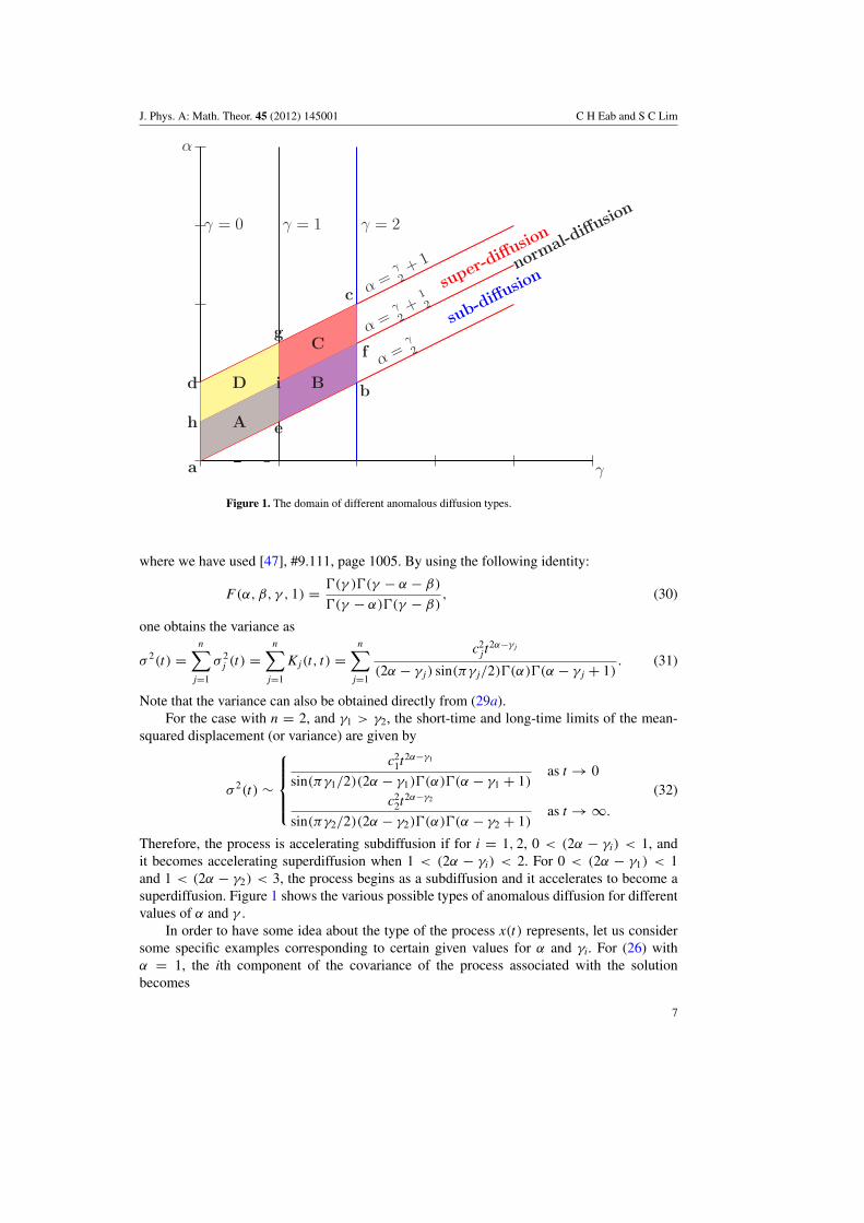
Figure 1. The domain of different anomalous diffusion types.

where we have used [47], #9.111, page 1005. By using the following identity:

F(α, β, γ , 1) = �(γ )�(γ − α − β)

�(γ − α)�(γ − β), (30)

one obtains the variance as

σ 2(t) =n∑

j=1

σ 2j (t) =

n∑j=1

Kj(t, t) =n∑

j=1

c2j t

2α−γ j

(2α − γ j) sin(πγ j/2)�(α)�(α − γ j + 1). (31)

Note that the variance can also be obtained directly from (29a).For the case with n = 2, and γ1 > γ2, the short-time and long-time limits of the mean-

squared displacement (or variance) are given by

σ 2(t) ∼

⎧⎪⎪⎨⎪⎪⎩c2

1t2α−γ1

sin(πγ1/2)(2α − γ1)�(α)�(α − γ1 + 1)as t → 0

c22t2α−γ2

sin(πγ2/2)(2α − γ2)�(α)�(α − γ2 + 1)as t → ∞.

(32)

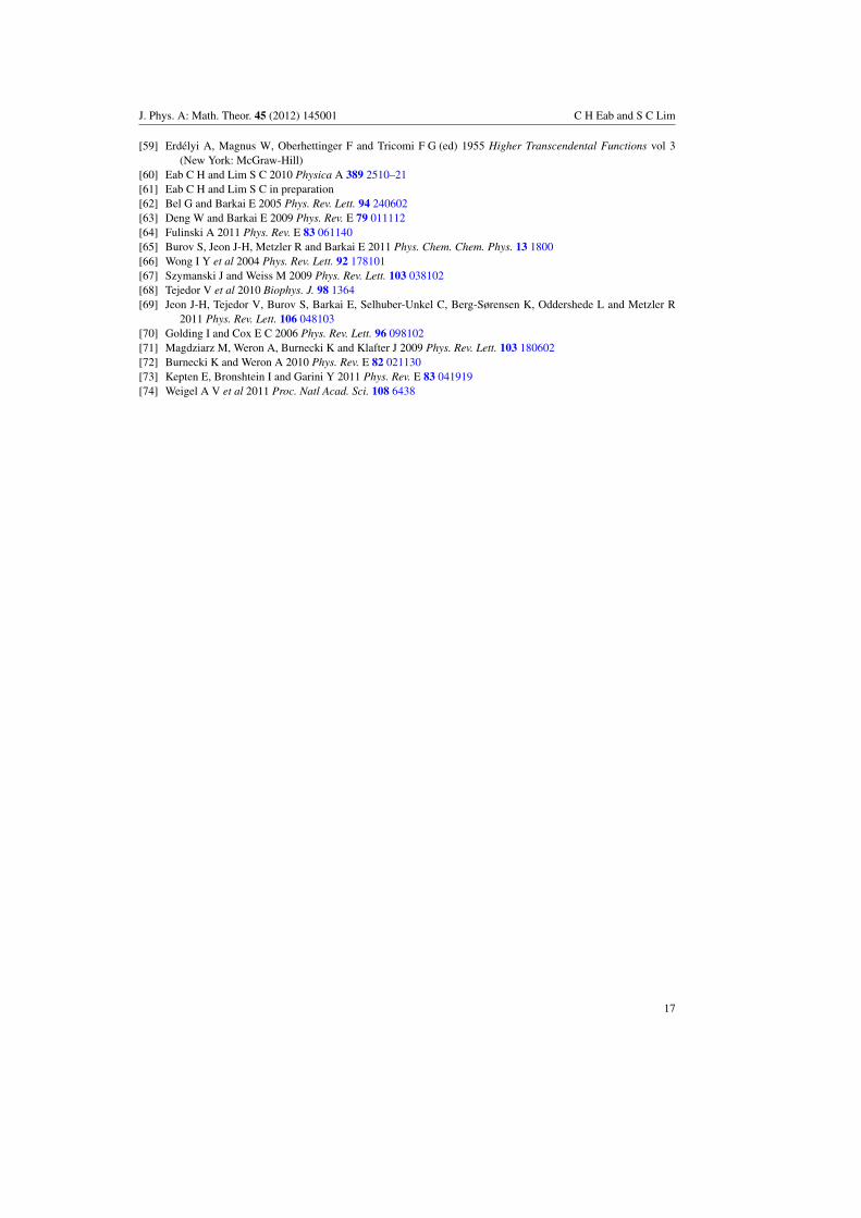
Therefore, the process is accelerating subdiffusion if for i = 1, 2, 0 < (2α − γi) < 1, andit becomes accelerating superdiffusion when 1 < (2α − γi) < 2. For 0 < (2α − γ1) < 1and 1 < (2α − γ2) < 3, the process begins as a subdiffusion and it accelerates to become asuperdiffusion. Figure 1 shows the various possible types of anomalous diffusion for differentvalues of α and γ .

In order to have some idea about the type of the process x(t) represents, let us considersome specific examples corresponding to certain given values for α and γi. For (26) withα = 1, the ith component of the covariance of the process associated with the solutionbecomes

7

J. Phys. A: Math. Theor. 45 (2012) 145001 C H Eab and S C Lim

Ki(s, t) = c2i

2 sin(πγi/2)�(2 − γi)

∫ s

0[(t − u)1−γi + (t − u)1−γi ] du

= c2i

2 sin(πγi/2)�(3 − γi)[t2−γi + s2−γi − (t − s)2−γi ], (33)

which is the covariance of the fractional Brownian motion (up to a multiplicative constant).Thus the covariance of the process K(s, t) = ∑n

i=1 Ki(s, t) is the covariance of a mixedfractional Brownian motion (also called the fractional mixed fractional Brownian motion bysome authors) [48–50] which is the sum of n independent fractional Brownian motion

x(t) =n∑

i=1

ciBHi (t), (34)

where Hi = (2−γi)/2 is the Hurst index of the fractional Brownian motion BHi (t). Thus, in themixed fractional Brownian motion model, anomalous diffusion begins with a lower diffusionrate, which can be represented by the fractional Brownian motion of lower Hurst index, and itis subsequently accelerated and is described by fractional Brownian motion of a higher Hurstindex. It is interesting to note that if all Hi are not equal to 1/2 (that is when they are all notBrownian motion), then such a process is long-range dependent [51, 52]. The process satisfiesa generalization of self-similar property called mixed self-similarity in the following sense:

n∑i=1

BHi (rt)d=

n∑i=1

rHi BHi (t). (35)

The variance of the process is given by

σ 2(t) =n∑

j=1

c2j t

2Hj

sin(πHj)�(2Hj + 1). (36)

Just like the previous case, suffice to consider n = 2. For H2 > H1, the short- and long-timelimits of the MSD are

σ 2(t) ∼

⎧⎪⎪⎪⎨⎪⎪⎪⎩c2

1t2H1

sin(πH1)�(2H1 + 1)as t → 0,

c21t2H1

sin(πH2)�(2H2 + 1)as t → ∞.

(37)

Thus the process behaves as accelerating superdiffusion (or subdiffusion) for 1/2 < Hj < 1(or 0 < Hj < 1/2) with j = 1, 2.

Here, we would like to remark that there exists another process called the step fractionalBrownian motion [53–55] which can also be used to model both accelerating and retardinganomalous diffusion. Although the mixed fractional Brownian motion can only be used todescribe accelerating anomalous diffusion, its mathematical structure is comparatively simplerthan that of step fractional Brownian motion. It is also interesting to mention that the mixedfractional Brownian motion x(t) = B1/2+BH (t), t in a finite interval [0, T ], is a semimartingaleif H ∈ (3/4, 1), and it is equivalent to Brownian motion in law [48].

Next, we consider another special case with the exponents α and γi satisfying the conditionα − γi = 0 for a particular ith fractional Gaussian noise. Equation (29a) now becomes

Ki(s, t) = c2i

2 sin(πα/2)�(α)

∫ s

0[(s − u)α−1 + (t − u)α−1] du

= c2i

2 sin(πα/2)�(α + 1)[sα + tα − (t − s)α]. (38)

8

J. Phys. A: Math. Theor. 45 (2012) 145001 C H Eab and S C Lim

Since γi = 2 − 2Hi = α, the process with the above covariance is fractional Brownianmotion indexed by 2 − 2Hi. Note that the other components of covariance Kj(s, t), j �= i,are given by (29b); hence, they are not the fractional Brownian motion. The variance isgiven by

σ 2(t) = σ 2i (t) +

n∑j=1, j �=i

σ 2j (t)

= c2i tα

2 sin(πα/2)�(α + 1)

+n∑

j=1, j �=i

c2j t

2α−γ j

2 sin(πγ j/2)(2α − γ j)�(α)�(α − γ j + 1). (39)

In this case, the type of anomalous diffusion depends on the values of α and 2α−γ j. Assuming0 < γ j < 1, then for 0 < α < 1 and 0 < 2α − γ j < 1 one obtains accelerating subdiffusion;when 1 < α < 2 and 1 < 2α − γ j < 2, the process is accelerating superdiffusion. Theprocess accelerates (retards) from subdiffusion (superdiffusion) to become superdiffusion(subdiffusion) when 1 < α < 2 and 0 < 2α − γ j < 1 (or when 0 < α < 1 and1 < 2α − γ j < 2).

Finally, we note that if ξi is white noise, that is when γi = 1, then Ki(s, t) takes thefollowing form:

Ki(s, t) = c2j s

αtα−1

�(α + 1)�(α)F(1 − α, 1, 1 + α, s/t), (40)

which is just the covariance of ‘type II’ or the Riemann–Liouville fractional Brownian motion[20]. The variance for the process is given by

σ 2i (t) = 2c2

i t2α−1

(2α − 1)(�(α))2. (41)

For n = 2, γ1 = 1 and γ2 < 1, one obtains a process which is an accelerating subdiffusion if1/2 < α < 1, an accelerating superdiffusion if 1 < α < 3/2 and finally it represents a processwhich accelerates from a subdiffusion to a superdiffusion if 1/2α < 1 and γ2 < 2α − 1.

From the above discussion, it is noted that a simple fractional Langevin equation drivenby a single fractional Gaussian noise results in an anomalous diffusion. However, when theprocess is driven by more than single fractional Gaussian noise terms, the resulting processcan be accelerating subdiffusion or superdiffusion, depending on the fractional order of thenoise terms and the derivative term. Thus, the interplay between multiple driving fractionalGaussian noise terms in the fractional Langevin-like equation leads to a simple Gaussianmodel of accelerating anomalous diffusion.

4. Retarding anomalous diffusion

There exists another type of anomalous diffusion that slows down with time. In other words,for short times the mean-squared displacement of such a diffusion process varies as tα1 ,and it varies as tα2 with α2 < α1 for long times. Retarding anomalous diffusion occurs invarious physical and biological systems. For example, in the single-file diffusion that occursin cell membranes and narrow channels [56, 57] and the retarding anomalous diffusion insemiconductors [12, 58].

9

J. Phys. A: Math. Theor. 45 (2012) 145001 C H Eab and S C Lim

A simple Gaussian model for retarding anomalous diffusion can be obtained byconsidering a special case of (1) which takes the form of the following fractional stochasticdifferential equation:

a1Dα1 x(t) + a2Dα2 x(t) =n∑

h=1

c jξγ j (t), 0 < α2 < α1 < 2. (42)

For both Riemann–Liouville and Caputo cases, the Laplace transform of (42) gives

[a1 pα1 + a2 pα2 ]x(p) − B(p) =n∑

j=1

c j ξγ j (p), (43)

where B(p) is given by (15). For simplicity, we again choose the initial conditions such thatB(p) = 0. The Green function is then given by the inverse Laplace transform of

G(p) = 1

a1 pα1 + a2 pα2= 1

a1

p−α2

pα1−α2 + (a2/a1)(44)

such that its inverse Laplace transform gives

G(t) = 1

a1tα1−1Eα1−α2,α1

(−a2

a1tα1−α2

), (45)

where

Eμ,ν (z) =∞∑j=0

z j

�(μ j + ν), μ > 0, ν > 0, (46)

is the Mittag–Leffler function [59]. Using (20) and (21), and substituting C(t) =∑nj=1 c2

jt−γ j

�(1−γ j ), one obtains

GC(t) =n∑

j=1

c2j

∫ t

0du

1

a1(t − u)α1−1Eα1−α2,α1

(−a2

a1(t − u)α1−α2

)u−γ j

�(1 − γ j)

=n∑

j=1

c2j

a1tα1−γ j Eα1−α2,α1−γ j+1

(−a2

a1tα1−α2

). (47)

The covariance K(s, t) = ∑nj=1 c2

jKj(s, t) is given by (20) with

Kj(s, t) =∫ s

0du

[(s − u)α1−1

a1Eα1−α2,α1

(−a2

a1(s − u)α1−α2

)][

(t − u)α1−γ j

a1Eα1−α2,α1−γ j+1

(−a2

a1(t − u)α1−α2

)]

+∫ s

0du

[(t − u)α1−1

a1Eα1−α2,α1

(−a2

a1(t − u)α1−α2

)][

(s − u)α1−γ j

a1Eα1−α2,α1−γ j+1

(−a2

a1(s − u)α1−α2

)]. (48)

The variance is given by σ 2(t) = ∑nj=1 c2

jKj(t, t),

Kj(t, t) = 2∫ s

0du

[(t − u)α1−γ j−1

a21

Eα1−α2,α1

(−a2

a1(t − u)α1−α2

)

× Eα1−α2,α1−γ j+1

(−a2

a1(t − u)α1−α2

)]. (49)

10

J. Phys. A: Math. Theor. 45 (2012) 145001 C H Eab and S C Lim

Note that the covariance and variance given above cannot be evaluated. However, by using thefollowing asymptotic properties of Mittag–Leffler function [59],

Eμ,ν (−z) ∼ −N∑

n=1

(−1)n−1z−n

�(ν − nμ)+ O(|z|−1−N ), | arg(z)| <

(1 − μ

2

)π, z → ∞, (50)

and

Eμ,ν (−z) ∼ 1

�(ν)+ O(z), z → 0, (51)

it is possible to obtain the short- and long-time behaviors of the variance. In the case of singlefractional Gaussian noise, one has for γ < 2α2,

σ 2(t) ∼{t2α1−γ , t → 0t2α2−γ , t → ∞.

(52)

Since α1 > α2, the process is a retarding subdiffusion (or superdiffusion) if for i = 1, 2,0 < αi − γ /2 < 1/2 (or 1/2 < αi − γ /2 < 1). In the case when there are more than onenoise, the dominant terms for the short time limit and long time limit for the variance are∼ tmin(2α1−γ j ) and ∼ tmax(2α2−γ j ), respectively. Thus we see that the double-order fractionalstochastic equation driven by single fractional Gaussian noise can be used to model retardinganomalous diffusion. The lower order fractional derivative term in (42) plays the role of adamping term which slows down the diffusion.

The main disadvantage of using (42) for modeling retarding anomalous diffusion is that ingeneral the covariance and variance of the underlying process cannot be calculated explicitly.We would like to find a particular case of (42) such that its solution is a process with covarianceand variance that can be completely determined. For this purpose, we consider the followingdouble-order fractional Langevin-like equation:

a1Dα1 x(t) + a2Dα2 x(t) = c1ξ1(t) + c2ξ2(t), 0 < α2 < α1 < 2. (53)

The two independent fractional Gaussian noises ξ1(t) and ξ2(t) are chosen such that for t > sthey have zero mean and the following covariance:

〈ξi(t)ξ j(s)〉 = (t − s)ν−αi−1

�(ν − αi)δi j ≡ Ci(t − s)δi j, i, j = 1, 2. (54)

We remark that the fractional Gaussian noise with covariance given by (54) is selected basedon practical purposes as it gives the required results as well as provides a more manageablesolution to (53). As a result (54), one can verify that the Laplace transforms of the covarianceof the fractional Gaussian noise C(t) = c2

1C1(t)+ c22C2(t) and the Green function G(t) satisfy

the following relation:

G(p)C(p) = p−ν . (55)

The inverse Laplace transform of (55) is

G(t) ∗ C(t) = tν−1

�(ν). (56)

The covariance of the process associated with the solution of (53) can be calculated using (20)and (56):

K(s, t) =∫ s

0du

[G(t − u)

(s − u)ν−1

�(ν)+ G(s − u)

(t − u)ν−1

�(ν)

]

=∫ s

0du

[(t − u)α1−1

a1Eα1−α2,α1

(−a2

a1(t − u)α1−α2

)(s − u)ν−1

�(ν)

+ (s − u)α1−1

a1Eα1−α2,α1

(−a2

a1(s − u)α1−α2

)(t − u)ν−1

�(ν)

]. (57)

11

J. Phys. A: Math. Theor. 45 (2012) 145001 C H Eab and S C Lim

Its variance is given by the following series expansion:

σ 2(t) = 2∫ t

0du

[1

a1�(ν)(t − u)α1+ν−2Eα1−α2,α1

(−a2

a1(t − u)α1−α2

) ]

= 2

a1�(ν)

∞∑n=0

(−a2a1

)ntn(α1−α2)+α1+ν−1

(n(α1 − α2) + α1 + ν − 1)�(n(α1 − α2) + α1). (58)

From (58), one gets the short and long time limits of the variance as

σ 2(t) ∼

⎧⎪⎨⎪⎩2

a1�(ν)�(α1)�(α1 + ν − 1)tα1+ν−1, t → 0

2

a1�(ν)�(α2)�(α2 + ν − 1)tα2+ν−1, t → ∞

. (59)

The process with covariance (58) and variance (59) is a retarding subdiffusion or superdiffusiondepending on the on the values of αi +ν −1, i = 1, 2. Thus, one can regard the term a2Dα2 x(t)in (53) as a damping term which slows down the anomalous diffusion.

A special case for which the covariance has a closed form is when ν = 1. For t > s, thecovariance (57) becomes

K(t, s) =∫ s

0du

[1

a1(t − u)α1−1Eα1−α2,α1

(−a2

a1(t − u)α1−α2

)

+ 1

a1(s − u)α1−1Eα1−α2,α1

(−a2

a1(s − u)α1−α2

) ]

= tα1

a1Eα1−α2,α1+1

(−a2

a1tα1−α2

)+ sα1

a1Eα1−α2,α1+1

(−a2

a1sα1−α2

)− (t − s)α1

a1Eα1−α2,α1+1

(−a2

a1(t − s)α1−α2

). (60)

It is interesting to note that the covariance consists of three terms of Mittag–Leffler functions ofsame order, and the time variables t and s enter the covariance expression (60) in a form similarto that of the fractional Brownian motion. Thus, it is not a coincidence that the asymptoticshort and long time limits of the covariance are given by

K(t, s) =

⎧⎪⎪⎨⎪⎪⎩1

a1�(α1 + 1)[tα1 + sα1 − |t − s|α1 ], t, s → 0

1

a2�(α2 + 1)[tα2 + sα2 − |t − s|α2 ], t, s, |t − s| → ∞.

(61)

Note that these are just the covariance of fractional Brownian motion indexed respectively byα1/2 = 1 − H1 and α2/2 = 1 − H2, with 0 < Hi < 1, i = 1, 2. Since both the short and longtime limits are the fractional Brownian motion, one can conclude that the stochastic processin this case is long-range dependent except when α1 = α2 = 1/2 or when both the limitingprocesses are the Brownian motion [51, 52].

The variance is given by

σ 2(t) = 2

a1tα1 Eα1−α2,α1+1

(−a2

a1tα1−α2

). (62)

The long and short time limits are given by

σ 2(t) ∼

⎧⎪⎪⎨⎪⎪⎩2

a1�(α1 + 1)tα1 , t → 0

2

a2�(α2 + 1)tα2 , t → ∞

. (63)

12

J. Phys. A: Math. Theor. 45 (2012) 145001 C H Eab and S C Lim

From the above results, one has for 0 < α2 < α1 < 1 a subdiffusion process which slowsdown with time, or a retarding subdiffusion. On the other hand, if 1 < α2 < α1 < 2, theprocess is a retarding superdiffusion.

It would be interesting to see whether (53) can be used to describe accelerating anomalousdiffusion as well. Suppose we replace condition (55) by the following:

G(p)C(p) = p−ν + p−κ , (64)

such that

C(p) = a1 pα1−ν + a1 pα1−κa2 pα2−ν + a2 pα2−κ . (65)

Inverse Laplace transform of (65) gives

C(t) = a1

[tν−α1−1

�(ν − α1)+ tκ−α1−1

�(κ − α1)

]+ a2

[tν−α2−1

�(ν − α2)+ tκ−α2−1

�(κ − α2)

]. (66)

The variance of the resulting process is

σ (t) = σ 2ν (t) + σ 2

κ (t), (67)

with σ 2ν (t) given by (58) and similarly for σ 2

κ (t) with ν replaced by κ . Thus for ν < κ , oneobtains

σ 2(t) ∼

⎧⎪⎪⎪⎨⎪⎪⎪⎩2

a1�(ν)�(α1)�(α1 + ν − 1)tα1+ν−1, t → 0

2

a2�(κ)�(α2)�(α2 + κ − 1)tα2+κ−1, t → ∞

. (68)

It is interesting to note that the process with the above variance represents acceleratingsubdiffusion if α1 + ν < α2 + κ , or κ > α1 − α2 + ν > 2α1 − α2. However, to achievesuch an accelerating subdiffusion it is necessary to consider four fractional Gaussian noiseterms in (53), a situation that may be difficult to realize in practice.

On the other hand, we recall that for (42) with more than one fractional Gaussian noise,the dominant term of the variance for the associated process in the short and long time limitsrespectively varies as tmin(2α1−γ j ) and tmax(2α2−γ j ), respectively. If we consider the case withα1 > α2 and γ1 > γ2, one then has 2α1 −γ2 > 2α1 −γ1 and 2α2 −γ2 > 2α2 −γ1. As a result,

σ 2(t) ∼{

t2α1−γ1 , t → 0t2α2−γ2 , t → ∞.

(69)

Thus, it is possible to use (53) to model accelerating anomalous diffusion provided 2α2 −γ2 >

2α1 − γ1 or α1 −α2 < (γ1 − γ2)/2. In other words, the fractional stochastic equation (53) canbe used to model retarding and accelerating anomalous diffusion by an appropriate choice ofthe order of the fractional derivatives and fractional Gaussian noise terms. Note that retardingdiffusion such as single-file diffusion can also be modeled by the fractional generalizedLangevin equation [60].

5. Concluding remarks

We have shown that it is possible to model both accelerating and retarding anomalous diffusionby using fractional Langevin-like stochastic differential equations driven by one or moreterms of fractional Gaussian noise. The solutions associated with some specific cases ofthese equations turn out to be some interesting processes in the short- and long-time limits.For example, two types of fractional Brownian motion, namely the usual standard fractionalBrownian motion and the Riemann–Liouville fractional Brownian motion are the asymptotic

13

J. Phys. A: Math. Theor. 45 (2012) 145001 C H Eab and S C Lim

processes of special cases of the model. This model also includes another interesting process,namely the mixed fractional Brownian motion, which is a simple process for describingaccelerating sub- and super-diffusion.

We note that the stochastic differential equations in our model can be regarded as thefractional Langevin-like equation of distributed order (10) with the weight function consistingof delta functions. One may want to consider cases with different types of weight functionsin (10), such as uniform or power-law weight functions. However, the results of our previousstudy on fractional Langevin equations of distributed order with uniform and power-law typeof weight functions indicate that such equations in general do not have closed solutions evenfor the case of simple fractional Langevin of distributed order driven by white noise [33].One thus expects the situation to be even more complex when weight functions other than thedelta functions are used for the multi-term fractional Langevin equation with more than onefractional noise terms.

One question of interest is that whether it is possible to model accelerating and retardinganomalous diffusion based on (26) and (42), using different Gaussian noise. If one is onlyinterested in the asymptotic limits of the mean-squared displacement of the stochastic process,then instead of using fractional Gaussian noise in the stochastic differential equations (26)and (42), Gaussian noise with covariance which has the ‘correct’ asymptotic limits ofpower-law type can be used. For example, for Gaussian noise with covariance which variesas Atμ−2/(1 + Atμ−ν/B), A and B are positive constants, 0 < μ, ν < 2. Such a covariancehas respectively short and long time limits Atμ−2 and Btν−2, respectively. Another example isthe noise of Mittag–Leffler type with covariance that of the form Atμ−2Eμ−ν,μ+1(−Atμ−ν/B),μ > ν, which has short- and long-time asymptotic limits Atμ−2/�(μ+1) and Btν−2/�(ν+1),

respectively. These two examples give the possible alternatives to the fractional Gaussian noiseξγ j as the driving noise. More discussion related to these cases will be given in a forthcomingpaper [61].

The usual characterization of anomalous diffusion uses its mean-squared displacement (orvariance in the context of this paper). However, it is well known that even for a Gaussian modelmean-squared displacement does not determine completely the underlying stochastic processand hence the mechanism of the anomalous diffusion. Recent advances in particle trackingdevices allow experiments to track the trajectories of a single molecule or nanoparticle incomplex systems such as cells in a biological system. Mean-squared displacement obtainedfrom the time series data gives the scaling exponent of the anomalous diffusion undertakenby such particles. Comparison of the experimental data so obtained with various models ofanomalous diffusion allows one to distinguish the different possible subdiffusion mechanisms.In particular, information of single-particle trajectories allows one to test the validity of ergodicproperty of the associated diffusion process. A stochastic process is said to be ergodic if theensemble average of certain physical quantity such as mean-squared displacement measuredin bulk coincides with the time average of the same quantity over sufficiently long time fromthe single-molecule time series. The examples of the ergodic process are Brownian motion andthe standard fractional Brownian motion. Another process of interest which is ergodic is themixed fractional Brownian motion which is the sum of two independent fractional Brownianmotions. On the other hand, the Riemann–Liouville fractional Brownian motion and heavytailed continuous-time random walk are non-ergodic [62–65].

By using the single-molecule data, the comparisons of experimental data based on variousmodels of anomalous diffusion such as the continuous-time random walk, fractional Brownianmotion, fractional Levy stable motion, etc have been carried out by various authors recently[66–73]. For example, diffusion of beads in the entangled F-actin networks at shorter timesexhibits continuous-time random walk behavior [66] . However, the analysis of the data of the

14

J. Phys. A: Math. Theor. 45 (2012) 145001 C H Eab and S C Lim

anomalous diffusion in crowded intracellular fluid such as cytoplasm of living cells rules outcontinuous-time random walk and favors the fractional Brownian motion [67]. The analysisof single-particle tracking data of lipid granules in yeast cells by Tejedor et al [68] seems torule out continuous-time random walk and shows agreement with fractional Brownian motion,but a subsequent study [69] shows that at short times the granules perform continuous-timerandom walk subdiffussion, while at longer times the motion is consistent with the fractionalBrownian motion. Various analyses of the biological data describing the motion of individualfluorescently labeled mRNA molecules inside live E. coli cells, a well-known experiment firstconducted by Golding and Cox [70], do not lead to the consensus result. Magdziarz et al [71]showed the fractional Brownian motion as the underlying stochastic process, but subsequentlyBurnecki and Weron claimed that the data follow fractional Levy stable motion [72]. Accordingto Kepten et al , the experiments on telomeres in the nucleus of the mammalian cell exhibit thefractional Brownian motion [73]. Recent study by Weigel et al [74] on the physical mechanismunderlying Kv2.1 voltage gated potassium channel anomalous dynamics using single-moleculetracking showed that both ergodic (diffusion on a fractal) and non-ergodic (continuous-timerandom walk) processes co-exist in the plasma membrane. Although it is widely recognizedthat the diffusion pattern of membrane protein displays anomalous subdiffusion, there is stillno agreement on the mechanisms responsible for this transport behavior. Currently, there isstill no consensus on whether heavy-tailed continuous-time random walk, fractional Brownianmotion, fractional Levy stable motion or some other stochastic processes can provide thecorrect description to anomalous diffusion in some biological systems. Thus, it is important tomake use of data and information other than the mean-squared displacement or the anomalousdiffusion exponent to determine the type of mechanism and the stochastic process describingthe anomalous diffusion. We hope that some of the processes considered in this paper may beof relevance in describing the anomalous diffusion in biological systems.

Finally, we remark that it would be interesting to investigate the Fokker–Planck equationsassociated with the processes considered in this paper. The mean first passage time for someof the simpler cases can also be studied [61].

Acknowledgments

SCL would like to thank the Malaysian Ministry of Science, Technology and Innovation andMalaysian Academy of Sciences for the support under the Brain Gain Malaysia (Back to Lab)Program. He would also like to thank Eli Barkai and Ralf Metzler for their useful commentson the ergodic property for the anomalous diffusion in various biological systems.

References

[1] Metzler R and Klafter J 2000 Phys. Rep. 339 1–77[2] Klages R, Radons G and Sokolov I M (ed) 2008 Anomalous Transport: Foundations and Applications (New

York: Wiley)[3] Klafter J, Lim S C and Metzler R (ed) 2011 Fractional Dynamics: Recent Advances (Singapore: World Scientific)[4] Seshadri V and West B J 1982 Proc. Natl Acad. Sci. USA 79 4501–5[5] Karger J and Ruthven D M 1992 Diffusion in Zeolites and other Microporous Solids (New York: Wiley)[6] Saxton M J 1996 Biophys. J. 70 1250[7] Weiss M, Elsner M, Kartberg F and Nilsson T 2004 Biophys. J. 87 3518[8] Khan S, Reynolds A M, Morrison I E G and Cherry R J 2005 Phys. Rev. E 71 041915[9] Bronstein I et al 2009 Phys. Rev. Lett. 103 018102

[10] Bergholz W, Hutchison J L and Pirouz P 1985 J. Appl. Phys. 58 3419–24[11] Agarwal A, Gossmann H J, Eaglesham D J, Herner S B and Fiory A T 1999 Appl. Phys. Lett. 74 2435

15

J. Phys. A: Math. Theor. 45 (2012) 145001 C H Eab and S C Lim

[12] Tan T Y and Gosele U 2005 Diffusion in Condensed Matter: Methods, Materials, Models 2nd edn ed P Heitjansand J Karger (New York: Springer) pp 165–208

[13] Kirk J G, Duffy P and Gallant Y A 1996 Astron. Astrophys. 314 1010[14] Perri S and Zimbardo G 2007 Astrophys. J. Lett. 671 L177[15] Geisel T, Nierwetberg J and Zacheri A 1985 Phys. Rev. Lett. 54 616[16] Furtado F, Glimm J, Lindquist B, Pereira F and Zhang Q 1992 Time Dependent Anomalous Diffusion for Flow

in Multi-Fractal Porous Media vol 398 (New York: Springer) p 79[17] Glimm J, Lindquist W B B, Pereira F and Zhang Q 1993 Transp. Porous Media 13 97–122[18] Peiltier R and Levy Vehel J 1995 Rapport Technique Inria 2645[19] Benassi A, Jaffard S and Roux D 1997 Rev. Mat. Iberoamericana 13 19[20] Lim S C 2001 J. Phys. A: Math. Gen. 34 1301–10[21] Ross B and Samko S 1993 Integral Trans. Spec. Funct. 1 277–300[22] Samko S 1995 Anal. Math. 21 213–36[23] Lorenzo C F and Hartley T T 2002 Nonlinear Dyn. 29 57–98[24] Kobelev Ya L, Kobelev L Ya and Klimontovich Yu L 2003 Dokl. Phys. 48 264–8[25] Chechkin A V, Gorenflo R and Sokolov I M 2005 J. Phys. A.: Math Gen. 38 L679–84[26] Sun H, Chen W and Chen Y Q 2009 Physica A 297 4586–92[27] Caputo M 1967 J. R. Astron. Soc. 13 529–39[28] Caputo M 2001 Fract. Calc. Appl. Anal. 4 421–42[29] Chechkin A, Gorenflo R and Sokolov I 2002 Phys. Rev. E 66 046129[30] Chechkin A V, Gorenflo R, Sokolov I M and Gonchar V Y 2002 Fract. Calc. Appl. Anal. 6 259–79[31] Meerschaert M M and Scheffler H P 2006 Stoch. Process. Appl. 116 1215–35[32] Mainardi F, Mura A, Pagnini G and Gorenflo R 2008 J. Vib. Control 14 1267–90[33] Eab C H and Lim S C 2011 Phys. Rev. E 83 031136[34] Samko S, Kilbas A A and Maritchev D I 1993 Integrals and Derivatives of the Fractional Order and Some of

Their Applications (Armsterdam: Gordon and Breach)[35] Podlubny I 1999 Fractional Differential Equations (San Diego: Academic)[36] West B, Bologna M and Grigolini P 2003 Physics of Fractal Operators (New York: Springer)[37] Kilbas A A, Srivastava H M and Trujillo J J 2006 Theory and Applications of Fractional Differential Equations

(Amsterdam: Elsevier)[38] Mainardi F 2010 Fractional Calculus and Waves in Linear Viscoelasticity (London: Imperial College Press)[39] Gelfand I M and Shilov G E 1964 Generalized Functions: Properties and Operations vol 1 (New York:

Academic)[40] Gelfand I M and Vilenkin N Ya 1964 Generalized Functions: Applications of Harmonic Analysis vol 4 (New

York: Academic)[41] Qian H 2003 Processes with Long Range Correlations (Lecture Notes in Physics vol 621) ed G Rangarajan and

M Ding (New York: Springer) p 22[42] Barton R J and Poor H V 1988 IEEE Trans. Inform. Theory 34 943–59[43] Zinde-Walsh V and Phillips P C B 2003 Probability, Statistics and Their Applications: Papers in Honor of Rabi

Bhattacharya ed K Athreya et al (Beachwood, OH: Institute of Mathematical Statistics) pp 285–92[44] Mushura Y 2008 Stochastic Calculus for Fractional Brownian Motion and Related Processes (Lecture Notes in

Mathematics vol 1929) (New York: Springer)[45] F Biagini Y H and Oksendal B 2008 Stochastic Calculus for Fractional Brownian Motion and Applications

(New York: Springer)[46] Azmoodeh E, Tikanmaki H and Valkeila E 2010 Stat. Probab. Lett. 80 1543–50[47] Gradshteyn I S and Ryzhik I M 1994 Table of Integrals, Series, and Products 5th edn (New York: Academic)[48] Cheridito P 2001 Bernoulli 7 913–34[49] El-Nouty C 2003 Stat. Probab. Lett. 65 111–20[50] Thale C 2009 Appl. Math. Sci. 3 1885–901[51] Doukhan P, Oppenheim G and Taqqu M S (ed) 2003 Theory and Applications of Long-Range Dependence

(New York: Birkhauser)[52] Lim S C and Muniandy S V 2003 J. Phys. A: Math. Gen. 36 3961[53] Benassi A, Bertrand P, Cohen S and Istas J 2000 Stat. Inference Stoch. Process. 3 101[54] Ayache A, Bertrand P and Levy Vehel J 2007 Stat. Inference Stoch. Process. 10 1[55] Lim S C and Teo L P 2009 J. Stat. Mech. 2009 P08015[56] Vestergaard-Bogind B, Stampe P and Christophersen P 1985 J. Membr. Bio. 88 67–75[57] Wei Q H, Bechinger C and Leiderer P 2000 Science 287 625–7[58] Servidori M et al 1987 J. Appl. Phys. 61 1834–40

16

J. Phys. A: Math. Theor. 45 (2012) 145001 C H Eab and S C Lim

[59] Erdelyi A, Magnus W, Oberhettinger F and Tricomi F G (ed) 1955 Higher Transcendental Functions vol 3(New York: McGraw-Hill)

[60] Eab C H and Lim S C 2010 Physica A 389 2510–21[61] Eab C H and Lim S C in preparation[62] Bel G and Barkai E 2005 Phys. Rev. Lett. 94 240602[63] Deng W and Barkai E 2009 Phys. Rev. E 79 011112[64] Fulinski A 2011 Phys. Rev. E 83 061140[65] Burov S, Jeon J-H, Metzler R and Barkai E 2011 Phys. Chem. Chem. Phys. 13 1800[66] Wong I Y et al 2004 Phys. Rev. Lett. 92 178101[67] Szymanski J and Weiss M 2009 Phys. Rev. Lett. 103 038102[68] Tejedor V et al 2010 Biophys. J. 98 1364[69] Jeon J-H, Tejedor V, Burov S, Barkai E, Selhuber-Unkel C, Berg-Sørensen K, Oddershede L and Metzler R

2011 Phys. Rev. Lett. 106 048103[70] Golding I and Cox E C 2006 Phys. Rev. Lett. 96 098102[71] Magdziarz M, Weron A, Burnecki K and Klafter J 2009 Phys. Rev. Lett. 103 180602[72] Burnecki K and Weron A 2010 Phys. Rev. E 82 021130[73] Kepten E, Bronshtein I and Garini Y 2011 Phys. Rev. E 83 041919[74] Weigel A V et al 2011 Proc. Natl Acad. Sci. 108 6438

17