Embed Size (px)
Citation preview
Clemson UniversityTigerPrints
All Dissertations Dissertations
12-2017
Acceleration of High-Fidelity Wireless NetworkSimulationsMadhabi ManandharClemson University
Follow this and additional works at: https://tigerprints.clemson.edu/all_dissertations
This Dissertation is brought to you for free and open access by the Dissertations at TigerPrints. It has been accepted for inclusion in All Dissertations byan authorized administrator of TigerPrints. For more information, please contact [email protected].
Recommended CitationManandhar, Madhabi, "Acceleration of High-Fidelity Wireless Network Simulations" (2017). All Dissertations. 2054.https://tigerprints.clemson.edu/all_dissertations/2054
Acceleration of High-Fidelity Wireless NetworkSimulations
A Dissertation
Presented to
the Graduate School of
Clemson University
In Partial Fulfillment
of the Requirements for the Degree
Doctor of Philosophy
Electrical Engineering
by
Madhabi Manandhar
December 2017
Accepted by:
Dr. Daniel L. Noneaker, Committee Chair
Dr. Harlan B. Russell, Committee Co-Chair
Dr. Melissa C. Smith
Dr. James Martin
Abstract
Network simulation with bit-accurate modeling of modulation, coding and
channel properties is typically computationally intensive. Simple link-layer models
that are frequently used in network simulations sacrifice accuracy to decrease simu-
lation time. We investigate the performance and simulation time of link models that
use analytical bounds on link performance and bit-accurate link models executed in
Graphical Processing Units (GPUs). We show that properly chosen analytical bounds
on link performance can result in simulation results close to those using bit-level sim-
ulation while providing a significant reduction in simulation time. We also show that
bit-accurate decoding in link models can be expedited using parallel processing in
GPUs without compromising accuracy and decreasing the overall simulation time.
ii

Acknowledgments
I would like to thank my advisor Dr. Daniel Noneaker for his guidance and
support all through my graduate studies in Clemson. I would also like to thank Dr.
Harlan Russell, Dr. Melissa Smith and Dr. James Martin for taking the time to serve
as members of my committee and helping me with my dissertation.
A special thank you to my friends here in Clemson and back home for their
help and support. And lastly, I thank my parents and my husband, Anjan for their
constant support and encouragement in all my pursuits.
iii
Table of Contents
Title Page . . . . . . . . . . . . . . . . . . . . . . . . . . . . . . . . . . . i
Abstract . . . . . . . . . . . . . . . . . . . . . . . . . . . . . . . . . . . . ii
Acknowledgments . . . . . . . . . . . . . . . . . . . . . . . . . . . . . . . iii
List of Tables . . . . . . . . . . . . . . . . . . . . . . . . . . . . . . . . . vi
List of Figures . . . . . . . . . . . . . . . . . . . . . . . . . . . . . . . . . vii
1 Introduction . . . . . . . . . . . . . . . . . . . . . . . . . . . . . . . . 1
2 Literature Review . . . . . . . . . . . . . . . . . . . . . . . . . . . . . 6
3 System Description . . . . . . . . . . . . . . . . . . . . . . . . . . . . 103.1 Small network . . . . . . . . . . . . . . . . . . . . . . . . . . . . . . . 113.2 Large network . . . . . . . . . . . . . . . . . . . . . . . . . . . . . . . 153.3 Approximations considered in the simulations . . . . . . . . . . . . . 18
4 Link Modeling with Off-Line Decoder Simulation . . . . . . . . . . 204.1 Stationary approximation of a mixed-distribution channel . . . . . . . 224.2 Network performance using link modeling with off-line decoder
simulation . . . . . . . . . . . . . . . . . . . . . . . . . . . . . . . . . 24
5 Approximations in On-Line Viterbi Decoder Simulation . . . . . . 345.1 Closed-form approximations to the probability of code-word error . . 355.2 Threshold-based approximation to the probability of code-word
error . . . . . . . . . . . . . . . . . . . . . . . . . . . . . . . . . . . . 365.3 Comparison of simulation results . . . . . . . . . . . . . . . . . . . . 37
6 GPU-Accelerated On-Line Viterbi Decoder Simulation . . . . . . 436.1 Introduction to GPUs . . . . . . . . . . . . . . . . . . . . . . . . . . 446.2 Memory organization in the GPU . . . . . . . . . . . . . . . . . . . . 466.3 Parallel Viterbi decoding . . . . . . . . . . . . . . . . . . . . . . . . . 486.4 Performance evaluation of various optimization techniques . . . . . . 56
iv
7 Network Simulation with GPU-Accelerated Viterbi Decoding . . 637.1 Accelerating network simulation with PBVD algorithm . . . . . . . . 647.2 Network simulation performance with the PBVD algorithm . . . . . . 66
8 Link Modeling in Large-Network Simulation . . . . . . . . . . . . . 768.1 Simulation performance with the various link models . . . . . . . . . 77
9 GPU-Based TDMP Decoding for LDPC codes . . . . . . . . . . . 859.1 WiMax-standard LDPC code . . . . . . . . . . . . . . . . . . . . . . 869.2 TDMP algorithm . . . . . . . . . . . . . . . . . . . . . . . . . . . . . 879.3 Implementing the TDMP algorithm on a GPU . . . . . . . . . . . . . 899.4 Performance evaluation of TDMP algorithm
using CPU and GPU . . . . . . . . . . . . . . . . . . . . . . . . . . . 90
10 Network Simulation with GPU-Accelerated TDMP Decoding . . 9610.1 Simulation of the small network with TDMP decoding . . . . . . . . 9710.2 Simulation of the large network with TDMP decoding . . . . . . . . . 100
11 Conclusion . . . . . . . . . . . . . . . . . . . . . . . . . . . . . . . . . 115
Appendices . . . . . . . . . . . . . . . . . . . . . . . . . . . . . . . . . . . 118A Computation complexity of Viterbi Algorithm . . . . . . . . . . . . . 119B Complexity of Viterbi decoding in ns-3 network simulation . . . . . . 121
Bibliography . . . . . . . . . . . . . . . . . . . . . . . . . . . . . . . . . . 123
v

List of Tables
3.1 Main flow and interfering flows in the large network for variousscenarios. . . . . . . . . . . . . . . . . . . . . . . . . . . . . . . . . . 17
4.1 Time for bit-accurate simulation of one second of network activity. . . 27
5.1 Link models for simulation systems considered. . . . . . . . . . . . . . 365.2 Time required to simulate 1s of elapsed time,
inter-flow distance=2400 m. . . . . . . . . . . . . . . . . . . . . . . . 40
7.1 Time required to simulate one second of network activity,inter-flow distance=2400 m. . . . . . . . . . . . . . . . . . . . . . . . 74
7.2 Time required to simulate one second of network activity with andwithout selective decoding, inter-flow distance=2400 m. . . . . . . . . 75
8.1 Time required to simulate 1s of elapsed time,main flow spanning at least 4 hops. . . . . . . . . . . . . . . . . . . . 81
10.1 Time required to simulate one second of network activity. . . . . . . . 11110.2 Time to simulate one second of elapsed time,
main flow spanning at least 3 hops. . . . . . . . . . . . . . . . . . . . 112
vi

List of Figures
3.1 5 node wireless ad hoc network. . . . . . . . . . . . . . . . . . . . . . 143.2 64 node ad hoc radio network. . . . . . . . . . . . . . . . . . . . . . . 16
4.1 Performance with Viterbi decoding and two Gaussian channelmodels. . . . . . . . . . . . . . . . . . . . . . . . . . . . . . . . . . . 29
4.2 Performance with TDMP decoding and two Gaussian channelmodels. . . . . . . . . . . . . . . . . . . . . . . . . . . . . . . . . . . 30
4.3 Throughput with bit-accurate and off-line table look-up Viterbidecoder simulation, node E located at (0, 3052). . . . . . . . . . . . . 31
4.4 Throughput with bit-accurate and off-line table look-up Viterbidecoder simulation, node E located at (0, 3352). . . . . . . . . . . . . 32
4.5 Throughput with bit-accurate and off-line table look-up TDMPdecoder simulation, node E located at (0, 3052). . . . . . . . . . . . . 33
5.1 Throughput of flow 1 for various inter-flow distances and twointerference probabilities, node E located at (0, 3052). . . . . . . . . . 41
5.2 Throughput of flow 1 for various inter-flow distances and twointerference probabilities, node E located at (0, 3352). . . . . . . . . . 42
6.1 GPU memory organization. . . . . . . . . . . . . . . . . . . . . . . . 476.2 Data flow for time step t in the forward-pass phase of the Viterbi
algorithm using a GPU. . . . . . . . . . . . . . . . . . . . . . . . . . 516.3 Data flow diagram for Viterbi decoding with post computation data
storage. . . . . . . . . . . . . . . . . . . . . . . . . . . . . . . . . . . 556.4 Packet error probability for packet size 16000 bits. . . . . . . . . . . . 606.5 Simulation time for packet sizes 16000 bits and 200 bits. . . . . . . . 616.6 Simulation time for packet sizes 2000 bits and 8000 bits. . . . . . . . 62
7.1 Throughput with PBVD (GPU) and bit-accurate Viterbi decoding(CPU), node E located at (0, 3352). . . . . . . . . . . . . . . . . . . . 69
7.2 Throughput with concurrent PBVD (GPU) and bit-accurate Viterbidecoding (CPU), node E located at (0, 3352). . . . . . . . . . . . . . 70
7.3 Throughput with selective PBVD (GPU) and selective bit-accurateViterbi decoding (CPU), node E located at (0, 3352). . . . . . . . . . 71
vii
7.4 Throughput with tighter concave-Chernoff bound and selective tighterconcave-Chernoff bound, node E located at (0, 3352). . . . . . . . . . 72
7.5 Throughput with concave integral bound and selective concave integralbound, node E located at (0, 3352). . . . . . . . . . . . . . . . . . . . 73
8.1 Comparison of mainflow’s throughput, mainflow spanningat least 3 hops . . . . . . . . . . . . . . . . . . . . . . . . . . . . . . . 82
8.2 Comparison of mainflow’s throughput, mainflow spanningat least 4 hops. . . . . . . . . . . . . . . . . . . . . . . . . . . . . . . 83
8.3 Comparison of mainflow’s throughput, mainflow spanningat least 5 hops. . . . . . . . . . . . . . . . . . . . . . . . . . . . . . . 84
9.1 Packet error probability for TDMP decoding of (2304,1152)LDPC code. . . . . . . . . . . . . . . . . . . . . . . . . . . . . . . . . 93
9.2 Simulation time for TDMP decoding of (2304,1152) LDPC code. . . . 949.3 Simulation time for early terminating TDMP decoding of (2304,1152)
LDPC code. . . . . . . . . . . . . . . . . . . . . . . . . . . . . . . . . 95
10.1 Throughput with TDMP decoding using a CPU and a GPU in thesmall network, node E located at (0, 3052). . . . . . . . . . . . . . . . 103
10.2 Throughput with bit-accurate TDMP decoding and with SINR thresh-old γ = 1.5 dB in the small network, node E located at (0, 3052). . . . 104
10.3 Throughput with bit-accurate TDMP decoding and with SINR thresh-old γ = 1.6 dB in the small network, node E located at (0, 3052). . . . 105
10.4 Throughput with TDMP decoding using a CPU and a GPU in thesmall network, node E located at (0, 3352). . . . . . . . . . . . . . . . 106
10.5 Throughput with bit-accurate TDMP decoding and with SINR thresh-old γ = 1.5 dB in the small network, node E located at (0, 3352). . . . 107
10.6 Throughput with bit-accurate TDMP decoding and with SINR thresh-old γ = 1.6 dB in the small network, node E located at (0, 3352). . . . 108
10.7 Throughput with TDMP decoding using CPU and bit-accurate lookuptable, node E located at (0, 3052). . . . . . . . . . . . . . . . . . . . . 109
10.8 Throughput with TDMP decoding using CPU and bit-accurate lookuptable, node E located at (0, 3352). . . . . . . . . . . . . . . . . . . . . 110
10.9 Throughput of main flow, main flow spanning at least 3 hops. . . . . 11210.10Throughput of main flow, main flow spanning at least 4 hops. . . . . 11310.11Throughput of main flow, main flow spanning at least 5 hops. . . . . 114
viii
Chapter 1
Introduction
Ad hoc radio networks are widely used to provide reliable communication in
environments that lack physical communication infrastructure. The need for increased
efficiency in the use of the limited radio spectrum and the desire for a wider range of
services in wireless networks stimulates ongoing research into the development of pro-
tocols that provide greater spectral efficiency, increased end-to-end throughput, and
a better quality of service in ad hoc radio networks. Both research and development
require thorough testing of the various protocols, radio communication techniques,
and applications under consideration in a wide range of realistic operating conditions.
The difficulty and cost of achieving wide-ranging testing of a radio network
with hardware prototypes dictates extensive use of network simulation as a tool for
characterizing the performance achieved in the network. A well-designed network
simulation with an accurate bit-level model of each radio communication link in the
network can reflect the behavior of the actual network with high fidelity. The com-
ponents of each link include the format of its radio transmissions, the properties of
the radio channel, and the architecture and algorithms in its radio receiver.
Unfortunately, this level of fidelity comes at the cost of a complicated link
1
model which can result in extremely long simulations to obtain the desired per-
formance data. (The most computationally intensive part of an accurate bit-level
link model is frequently the implementation of the decoding algorithm for the error-
correction code used in the link transmission.) The network simulation time can be
reduced substantially if a link model of low complexity is used instead, but the time
savings comes at the cost of reduced accuracy in the results. This trade-off between
the fidelity and computation time in the simulation of an ad hoc radio network is the
focus of this dissertation, with particular attention paid to the choices in modeling
the radio links of the network and in the computational platform that is used to
implement the computationally intensive decoding algorithm for the link model.
Among the simplest link models used in a wireless network simulation is the
free-space path-loss model [1]. A radio transmission results in a signal power at a
receiving node in the network which is determined based on the antenna gains at the
transmitting node and the receiving node in the direction of the communication, the
distance-dependent path-loss model used for the channel, and the distance between
the two nodes. A transmission is treated as successful within the simulation if the
received power is greater than a predefined threshold. A drawback of this model is that
it does not take into account interference that might be present in the network during
the packet reception process. Alternatively, the distance between the transmitter and
the receiver can be used directly in the simulation to determine the success of a
transmission for given antenna gains and a given transmission format [2, 3]. In this
transmission range model, a transmitting node only communicates with a receiving
node that is within its “transmission range”.
Another link model regularly used in wireless network simulation is the cap-
ture threshold model [4]. Unlike the free-space path loss model, this model calculates
the signal-to-interference-plus-noise-ratio (SINR) at the receiver but accounts for only
2
one interferer at a time. The SINR for each interferer is calculated separately and
successful reception of a packet is only confirmed if all the SINRs are greater than
a designated threshold. This model is implemented in the ns-2 discrete-event net-
work simulator [5], and research focused on higher-layer protocols that uses ns-2 as
a network simulation tool often uses the default capture threshold model [6–8]. A
better approach is to consider the aggregate effect of all interferers in determining the
the received signal, which in fact reflects the true SINR at the receiver. The addi-
tive interference model [4] implements this by considering all the unwanted received
signals as equivalent Gaussian noise. A transmission is considered successful in this
model only if the received SINR is above a predetermined threshold. The additive
interference model is the default channel model in the ns-3 discrete-event network
simulator [9].
A more precise approach to link modeling accounts explicitly for the error-
correction coding and the corresponding decoding algorithm used in the link. This is
often the most computationally intensive part of bit-accurate link simulation, which
can be mitigated at the time of network simulation by use of a predetermined look-up
table for the probability of error at the decoder output. The look-up table is indexed
by one or a few simple link parameters, and if the index parameter provide sufficient
flexibility in the link scenarios that are reflected, the computation time to construct
the table can be amortized over many network simulations.
The computational cost of constructing a fine-resolution look-up table in-
creases with the range of transmission formats (error-correction code, modulation
format, packet size), types of interference environment, and decoding algorithms con-
sidered in the network simulations. Consequently, the bit-accurate link model is
often replaced by a simpler model that uses the additive interference model [10–12]
with a threshold chosen according to the modulation and coding used in the system.
3
Alternatively, some classes of links are amenable to analytical methods for deter-
mining a closed-form expression that gives or approximates the probability of error
in a link transmission. For example, bounds on the code-word error probability for
convolutional coding and hard-decision Viterbi decoding over an independent, iden-
tically distributed (i.i.d.) Gaussian noise channel is obtained using the first-event
error probability [13]. Similarly, bounds on the probability of code-word error that
are applicable to soft-decision Viterbi decoding for a broader class of Gaussian noise
channels is developed in [14]. Each provides flexibility in accounting for different
error-correction codes and packet lengths. The resulting expression can be evaluated
for each simulated link transmission as the basis for determining the outcome of that
transmission.
The development of the graphical processing units (GPU) as a tool for general-
purpose computing has helped stimulate increased interest in the use of hardware
parallel architectures for error-correction decoding. It has included investigations of
parallel implementation of Viterbi decoding for convolutional codes [15], [16], [17].
Some newer classes of error-correction codes, such as quasi-cyclic low-density parity-
check (LDPC) codes are designed specifically to support a high level of parallelism in
decoding algorithms for the codes [18], [19], [20]. This introduces the possibility of
incorporating parallel processing for error-correction decoding in a network simulation
as a component of bit-accurate link modeling in order to reduce the computation time
of the simulation.
The first part of this dissertation is focused on bit-accurate simulation of
Viterbi decoding of a convolutional code and approximations of the resulting error
probability using various analytical bounds. We analyze the effects of the resulting
link models on the accuracy of the simulation of a small ad hoc radio network. GPU-
based parallel processing of the Viterbi decoder and its implementation in the network
4
simulation is also examined. The analysis of link models and parallel processing is
extended to their use in the simulation of a large ad hoc radio network as well. In
the second part of the dissertation, the same questions are addressed for a network in
which LDPC codes are used in the link transmissions. GPU-based parallel implemen-
tation of a decoder for LDPC codes and its incorporation into a network simulation is
considered. The simulation tool ns-3 along with the external library it++ [21] is used
for all the network simulations, together with custom-developed modules for some of
the link-layer models.
The remainder of the report is organized in the following manner. A review
of related research is presented in Chapter 2. Chapter 3 describes the system and
channel considered in the dissertation. Chapter 4 is focused on the use of off-line
generated look-up tables of the probability of code-word error with Viterbi decoding
for convolutional codes and a decoding algorithm for LDPC codes. In Chapter 5,
the performance of the Viterbi decoder and its approximations using different types
of analytical bounds is studied. Chapter 6 and 7 address parallel implementation of
Viterbi decoding and its incorporation into ns-3. The various link models with Viterbi
decoding are considered in the context of the large network in Chapter 8. Parallel
decoding of LDPC codes and its implementation in ns-3 is presented in Chapters 9
and 10. And summary of conclusions from the research is presented in Chapter 11.
5
Chapter 2
Literature Review
Earlier studies on network layer research and scheduling algorithms did not
emphasize a lot on the channel models and interference present in the network. Since
detailed channel and interference models have higher complexity, these research only
focused on the network layout to design scheduling algorithm widely known as graph
based scheduling [22], [23], [24]. These algorithms provide transmission and schedul-
ing using the graph based approach that completely avoids secondary interference
in the network i.e. interference from other transmitters present nearby. Eventually
new research popularized the concept of interference-based scheduling that includes
interference present in the network to build more realistic scenarios. The difference
in performance using a graph based scheduling and a new scheduling that uses full
knowledge of the interference environment is shown in [25]. The interference model
computes the signal-to-interference ratio and adds an extra condition for the received
SIR to be greater than a threshold before allowing a set of links to transmit simul-
taneously. It concludes that by acknowledging the interference in the network, the
new scheduling can avoid poor channel conditions that results in better network per-
formance compared to the graph-based scheduling. In [26], the performance of a
6
graph-based scheduling algorithm on two different physical layer models namely the
Protocol Interference Model and Physical Interference Model is compared to show how
its performance deteriorates if a channel model that accounts for network interference
is used.
Newer network layer research use more developed interference models to cal-
culate the received SINR for more accurate results as seen in [27] and [28]. However,
these models assume communications are perfect if the received SINR is greater than
a predefined threshold. More precise results can be obtained if the received SINRs
are used to probabilistically determine if packets are received correctly or not, based
on the physical and link layers of the system. The importance of using accurate
physical layer models in wireless network simulations and uses a statistical approach
to develop empirical models for mobile wireless networks based on several field ex-
periments is discussed in [29]. Similarly, the differences in system performance when
using efficient simple models to a more computationally complex yet comprehensive
models like SIRCIM [30] is detailed in [31]. It emphasizes on the use of accurate
physical layer models that uses bit error rates for packet reception in wireless net-
work research and also presents ideas on parallel executions using scalable simulation
library GloMoSim [32]. An even more detailed discussion on the necessity of accurate
physical layer modeling of MANETs is given in [33]. It also compares the performance
of GloMoSim with ns-2.
Network simulators provide a convenient tool to simulate and examine wire-
less network protocols and applications. OPNET [34], network simulator 1, 2 and 3,
OMNET++ [35], GloMoSim, QualNet are some well known wireless network simu-
lators. Over the years network simulators have also seen development both in terms
of complexity and accuracy. Simulators like ns-3, OMNET++, OPNET, GloMoSim
have comprehensive interference and physical layer models. These simulators also
7
have BER based signal reception along with SNR threshold based reception. How-
ever, they don’t have bit-accurate implementation of link-layer models. Some of
them though have link layer models that use tables with packet error probabilities
for the link layer codes used, as shown in [36]. There have been studies to obtain
alternate ways to model the link-layer codes used without having to use tables or en-
coders and decoders in the network simulation [13]. The research provides an upper
bound on the code-word error probability for convolutional coding and hard-decision
Viterbi decoding over an independent, identically distributed (i.i.d.) Gaussian noise
channel. The upper bound obtained here can be easily implemented in a wireless
network simulator to carry out packet reception based on packet error probabilities
of the link-layer codes used. Similarly, upper bounds on the probability of code-word
error to soft-decision Viterbi decoding for Gaussian noise channels is developed in
[14] and bounds on Viterbi decoding in direct-sequence code-division multiple-access
(DS-CDMA) systems using binary convolutional coding, quaternary modulation with
quaternary direct-sequence spreading is developed in [37]. These bounds can also be
directly applied in the network simulators available.
The straightforward way to use bit-accurate link-layer models is to implement
bit-accurate decoders in network simulation. However, the large simulation time re-
quired by link-layer decoders discourage users to include them in network simulators.
There have been various researches to accelerate link-layer decoders. The idea of
parallely decoding Convolutional codes in software defined radio using GPUs is in-
troduced in [15]. It shows that Viterbi decoders can be sped up by carrying out the
calculations of each state in parallel by assigning the calculations of each state to a
single thread. The same parallel decoding is further accelerated in [16] by the tiled
Viterbi decoding algorithm (TVDA). TVDA divides each block of received words into
multiple chunks and carries out parallel Viterbi decoding as shown in [15] for each
8
of the chunk in parallel. After the calculations, the results from individual chunks
are merged to obtain a surviving path from the trellis. Another version of paral-
lel decoding of Viterbi codes referred to as the parallel block-based Viterbi decoder
(PBVD) implemented in CUDA is presented in [17]. The PBVD algorithm also di-
vides the received words into multiple chunks and carries out computations in the
individual chunks independently. The final merging step is not required in this algo-
rithm. Similarly parallel decoding of LDPC codes have also been a topic of interest
as LDPC codes are widely used in wireless network communications. The parallel
version of the belief propagation algorithm for decoding LDPC codes is presented in
[19]. Similarly a scalable and flexible implementation of LDPC decoder on a GPU
is shown in [20]. Furthermore, the turbo decoding message passing algorithm, which
is a form of layered belief-propagation algorithm is parallelized in [18]. It uses the
offset-min-sum TDMP algorithm to decode quasi-cyclic LDPC codes in parallel using
stream processors.
9

Chapter 3
System Description
We consider two ad hoc radio networks as examples for the numerical results in
this dissertation. The first network consists of four nodes with static single-hop routes
and a single non-coordinated source of interference. The network is referred to as the
small network, and it provides a simple scenario for gaining insights into the network-
level tradeoffs provided by the use of different methods of link-layer modeling and
simulation. The inter node distances in the small network are selectable parameters
which permit the identification of extremal conditions in the tradeoffs.
The second network contains 64 nodes and employs dynamic multiple-hop
routing. It is referred to as the large network. The performance of the large network
for different methods of link-layer modeling and simulation permits a comparison of
the tradeoffs among the different approaches when they are applied to the simulation
of an ad hoc radio network of practical interest. Performance results for each network
are obtained by simulating the network in ns-3 [9].
10
3.1 Small network
The topology of the small network is shown in Figure 3.1. Network nodes A, B,
C, and D are placed at the corners of a rectangle. Node A generates packets directed
to node C at a fixed rate. The data flow from node A to node C is referred to as flow
1. Similarly, node B generates packets for node D at a fixed rate, and the data flow
from node B to node D is called flow 2. The distance between nodes A and C is the
transmission distance, and the distance between nodes A and B is referred to as the
inter-flow distance. The transmission distance is fixed at 2600 m and the inter-flow
distance is varied from 2000 m to 5000 m to analyze various network conditions. Node
E is a non-coordinated transmitter (i.e., a jammer) located on the line that is the
perpendicular bisector of the line joining nodes A and B. If the line connecting nodes
A and B is considered as the x-axis and its perpendicular bisector is considered as
the y-axis, the location of node E can be expressed in Cartesian coordinates as (0, y).
All distances are expressed in meters, and the network performance is considered for
different values of the transmission distance and the inter-flow distance and for two
values of y.
The network nodes use the 802.11b [38] protocol with a maximum data-symbol
rate of 1 Mbps for both data and control messages. Nodes A and B transmit data
packets of size 2016 bytes which convey information from a constant-bit-rate source in
each of the two nodes. (Each source is implemented in the simulation by a constant-
bit-rate generator available in ns-3.) The data rate of each of the two sources, referred
to as the data generation rate, can be varied to generate data at a specified bit rate
up to the maximum. The media access control (MAC) sub-layer [39] is configured in
ad hoc mode [40]; so that each node is capable of operating as a router and is able to
both transmit and forward data packets. The nodes in the simulation for the small
11

network contain a trivial network layer, however, so that no dynamic routing occurs
in the example scenarios. The nodes use UDP [39] at the transport layer.
The ad hoc mode of the 802.11b MAC sub-layer uses an “RTS/CTS” protocol
in which the link’s data source node transmits a Ready-to-Send (RTS) control packet
addressed to its intended link destination mode to request reservation of the destina-
tion’s attention for a subsequent data packet transmission. If the intended destination
replies with a Clear-to-Send (CTS) control indicating it is available to receive a data
transmission, the source node transmits a data (DATA) packet addressed to the des-
tination node. If the destination node acquires the data packet, successfully detects
the data payload of the packet, and confirms that it is the intended recipient of the
packet, it returns an acknowledgment (ACK) packet to the data source node. The
CTS packet is also detected by third-party nodes in the network. It allows them to
recognize that a subsequent data packet transmission is imminent; thus, it serves the
additional function of reserving the channel in the local area of the intended destina-
tion for the duration of the packet data transmission. The control packet and data
packet transmissions are unslotted.
In the physical layer of each network node, the received word (i.e., symbol-
rate samples) for each data or control packet that is acquired are decoded based on
the system’s error-correction code. If the received word is not decoded correctly,
the packet is ignored. Each successfully detected physical-layer packet payload is
forwarded to the MAC sub-layer. The MAC sub-layer determines the MAC packet
type and its addressed destination. Each data and control packet not addressed to
the current node is used to update the node’s network allocation vector (NAV) and
then dropped, but the MAC-layer payload of a data packet addressed to the node is
passed to the next higher protocol layer. Each control packet addressed to the current
node is utilized in the MAC sub-layer as described in the previous paragraph.
12
In the physical layer of the node, an error-correction code is used to encode
each data or control packet in a single code word per packet. Two codes are con-
sidered here: the NASA standard rate-1/2, convolutional code [41] and the WiMax
standard rate-1/2, (2304,1152) low-density parity-check (LDPC) code [42]. Since
powerful LDPC codes of an appropriate length are not available for the (short) con-
trol packets, the convolutional code is used to encode the control packets even if the
data packets are encoded with the LDPC code. The physical layer also follows the
802.11b protocol with a few changes. Instead of differential binary phase-shift keyed
(differential BPSK) modulation, coded data bits are transmitted using BPSK direct-
sequence spread-spectrum (DS/SS) modulation with a spreading factor of NS = 22.
All transmissions occur with the same power.
The jammer, node E, uses a time-slotted transmission of data packets in time
slots of 3 s duration. The jammer is transmitting or silent in each of the sequence of
time slots according to a sequence of independent, identically distributed Bernoulli
random variables with a transmission probability p (the interference probability). The
transmitter power for the jammer is 8 dB more than the transmitter power for other
nodes in the network. The transmissions of node E use the same packet format
as the data packets transmitted by the network nodes. Node E does not transmit
802.11b control packets, and its transmissions are not addressed to any of the network
nodes. As p is increased, the four network nodes experience an increased probability of
interference from the jammer. Besides p, the location y of node E can also be changed
along the perpendicular bisector to alter the interference power at the network nodes.
The free-space channel is modeled by the Friis propagation equation [43]. Both
thermal noise with power spectral density N0
2and interference from other transmis-
sions affect the received signal. The interference power at a receiver from either the
jammer or other network nodes (or both) may vary within the reception interval of
13
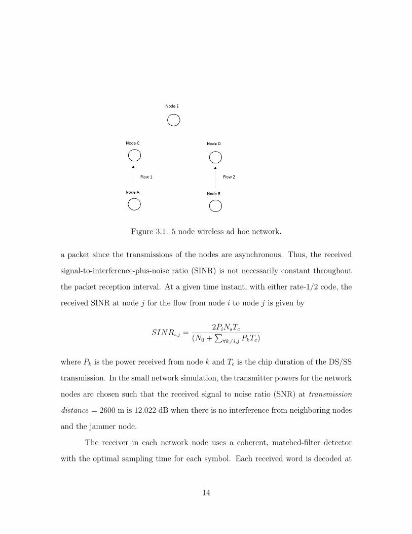
Figure 3.1: 5 node wireless ad hoc network.
a packet since the transmissions of the nodes are asynchronous. Thus, the received
signal-to-interference-plus-noise ratio (SINR) is not necessarily constant throughout
the packet reception interval. At a given time instant, with either rate-1/2 code, the
received SINR at node j for the flow from node i to node j is given by
SINRi,j =2PiNsTc
(N0 +∑
∀k =i,j PkTc)
where Pk is the power received from node k and Tc is the chip duration of the DS/SS
transmission. In the small network simulation, the transmitter powers for the network
nodes are chosen such that the received signal to noise ratio (SNR) at transmission
distance = 2600 m is 12.022 dB when there is no interference from neighboring nodes
and the jammer node.
The receiver in each network node uses a coherent, matched-filter detector
with the optimal sampling time for each symbol. Each received word is decoded at
14
the physical layer and passed to the MAC sub-layer. The throughput of each flow
is measured in the MAC sub-layer. Soft-decision Viterbi decoding [44] is used for
decoding each received word if the physical layer uses the convolutional code, and the
turbo-decoding message-passing (TDMP) algorithm [18] is used for decoding each
received word if the physical layer uses the LDPC code.
3.2 Large network
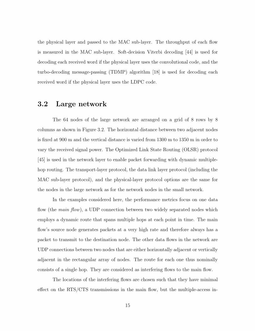
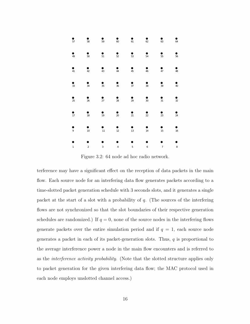
The 64 nodes of the large network are arranged on a grid of 8 rows by 8
columns as shown in Figure 3.2. The horizontal distance between two adjacent nodes
is fixed at 900 m and the vertical distance is varied from 1300 m to 1350 m in order to
vary the received signal power. The Optimized Link State Routing (OLSR) protocol
[45] is used in the network layer to enable packet forwarding with dynamic multiple-
hop routing. The transport-layer protocol, the data link layer protocol (including the
MAC sub-layer protocol), and the physical-layer protocol options are the same for
the nodes in the large network as for the network nodes in the small network.
In the examples considered here, the performance metrics focus on one data
flow (the main flow), a UDP connection between two widely separated nodes which
employs a dynamic route that spans multiple hops at each point in time. The main
flow’s source node generates packets at a very high rate and therefore always has a
packet to transmit to the destination node. The other data flows in the network are
UDP connections between two nodes that are either horizontally adjacent or vertically
adjacent in the rectangular array of nodes. The route for each one thus nominally
consists of a single hop. They are considered as interfering flows to the main flow.
The locations of the interfering flows are chosen such that they have minimal
effect on the RTS/CTS transmissions in the main flow, but the multiple-access in-
15
1 2 3 4 5 6 7 8
9 10 11 12 13 14 15 16
17 18 19 20 21 22 23 24
25 26 27 28 29 30 31 32
33 34 35 36 37 38 39 40
41 42 43 44 45 46 47 48
49 50 51 52 53 54 55 56
57 58 59 60 61 62 63 64
Figure 3.2: 64 node ad hoc radio network.
terference may have a significant effect on the reception of data packets in the main
flow. Each source node for an interfering data flow generates packets according to a
time-slotted packet generation schedule with 3 seconds slots, and it generates a single
packet at the start of a slot with a probability of q. (The sources of the interfering
flows are not synchronized so that the slot boundaries of their respective generation
schedules are randomized.) If q = 0, none of the source nodes in the interfering flows
generate packets over the entire simulation period and if q = 1, each source node
generates a packet in each of its packet-generation slots. Thus, q is proportional to
the average interference power a node in the main flow encounters and is referred to
as the interference activity probability. (Note that the slotted structure applies only
to packet generation for the given interfering data flow; the MAC protocol used in
each node employs unslotted channel access.)
16
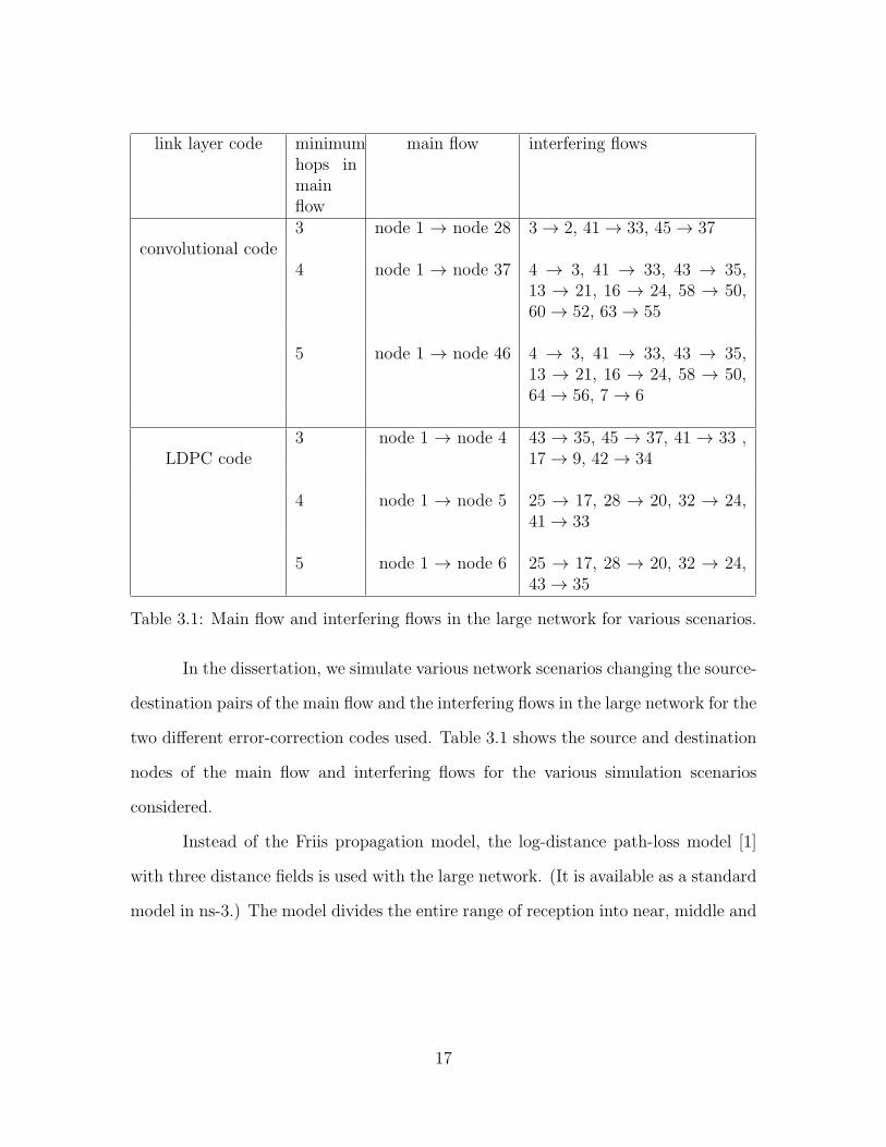
link layer code minimumhops inmainflow
main flow interfering flows
convolutional code3 node 1 → node 28 3 → 2, 41 → 33, 45 → 37
4 node 1 → node 37 4 → 3, 41 → 33, 43 → 35,13 → 21, 16 → 24, 58 → 50,60 → 52, 63 → 55
5 node 1 → node 46 4 → 3, 41 → 33, 43 → 35,13 → 21, 16 → 24, 58 → 50,64 → 56, 7 → 6
LDPC code3 node 1 → node 4 43 → 35, 45 → 37, 41 → 33 ,
17 → 9, 42 → 34
4 node 1 → node 5 25 → 17, 28 → 20, 32 → 24,41 → 33
5 node 1 → node 6 25 → 17, 28 → 20, 32 → 24,43 → 35
Table 3.1: Main flow and interfering flows in the large network for various scenarios.
In the dissertation, we simulate various network scenarios changing the source-
destination pairs of the main flow and the interfering flows in the large network for the
two different error-correction codes used. Table 3.1 shows the source and destination
nodes of the main flow and interfering flows for the various simulation scenarios
considered.
Instead of the Friis propagation model, the log-distance path-loss model [1]
with three distance fields is used with the large network. (It is available as a standard
model in ns-3.) The model divides the entire range of reception into near, middle and
17
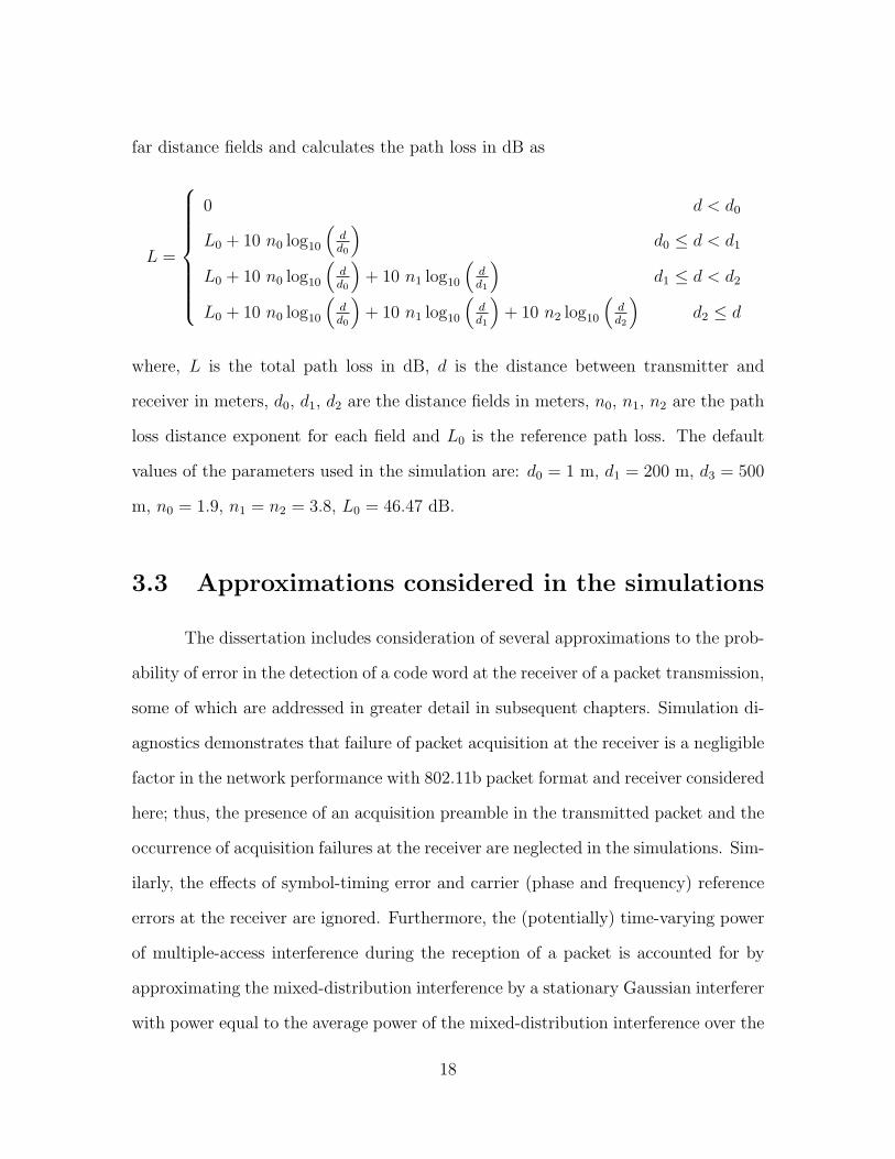
far distance fields and calculates the path loss in dB as
L =
0 d < d0
L0 + 10 n0 log10
(dd0
)d0 ≤ d < d1
L0 + 10 n0 log10
(dd0
)+ 10 n1 log10
(dd1
)d1 ≤ d < d2
L0 + 10 n0 log10
(dd0
)+ 10 n1 log10
(dd1
)+ 10 n2 log10
(dd2
)d2 ≤ d
where, L is the total path loss in dB, d is the distance between transmitter and
receiver in meters, d0, d1, d2 are the distance fields in meters, n0, n1, n2 are the path
loss distance exponent for each field and L0 is the reference path loss. The default
values of the parameters used in the simulation are: d0 = 1 m, d1 = 200 m, d3 = 500
m, n0 = 1.9, n1 = n2 = 3.8, L0 = 46.47 dB.
3.3 Approximations considered in the simulations
The dissertation includes consideration of several approximations to the prob-
ability of error in the detection of a code word at the receiver of a packet transmission,
some of which are addressed in greater detail in subsequent chapters. Simulation di-
agnostics demonstrates that failure of packet acquisition at the receiver is a negligible
factor in the network performance with 802.11b packet format and receiver considered
here; thus, the presence of an acquisition preamble in the transmitted packet and the
occurrence of acquisition failures at the receiver are neglected in the simulations. Sim-
ilarly, the effects of symbol-timing error and carrier (phase and frequency) reference
errors at the receiver are ignored. Furthermore, the (potentially) time-varying power
of multiple-access interference during the reception of a packet is accounted for by
approximating the mixed-distribution interference by a stationary Gaussian interferer
with power equal to the average power of the mixed-distribution interference over the
18
interval of the packet [14]. The stationary Gaussian approximation to multiple-access
interference is utilized in three approximations to the probability of code-word de-
tection error if the link is employing convolutional coding with soft-decision Viterbi
decoding.
The first of the decoder performance approximations, the tighter concave-
Chernoff bound [14], provides an upper bound on the probability of code-word error
under the stationary Gaussian approximation. The second of these uses the integral
form of the concave bound [14] (also referred to as the concave-integral bound), which
yields a tighter upper bound on the probability of code-word error than does the
tighter concave-Chernoff bound. With either approximation, a Bernoulli trail is con-
ducted for each packet transmission with a probability of packet error equal to the
probability of code-word error determined by the corresponding bound. The third
decoder performance approximation is an SINR-threshold based model in which re-
ceived packets are assumed to be detected correctly if the received SINR is greater
than a predetermined threshold γ but detected incorrectly otherwise.
A well-chosen cyclic redundancy check (CRC) outer code in the packet format
and a corresponding outer CRC decoder in the receiver results in a negligible prob-
ability of undetected code-word error. While the presence of the CRC encoder and
decoder is not incorporated into the simulations, it is assumed that each code-word
error at a receiver results in a known decoder failure, allowing the MAC layer to react
accordingly.
19
Chapter 4
Link Modeling with Off-Line
Decoder Simulation
The highest fidelity model of a link transmission in a network simulation em-
ploys (on-line) bit-level simulation of the detection of each transmission on each link.
The approach uses a simulation-generated sample outcome for each receiver symbol-
rate statistic for each transmission based on the transmission format, the type of
symbol-rate detection employed in the receiver, and the probabilistic model of the
underlying communications environment (i.e., the channel) for each link. It also em-
ploys bit-accurate implementation of error-correction decoding.
On-line bit-accurate simulation reflects the effect of correlation among the re-
ceiver statistics for a given transmission. In those instances when it is significant, the
simulation can also be designed to reflect correlation among the receiver statistics for
distinct transmissions on the link and among the statistics for transmissions on differ-
ent links. It permits great flexibility in examining the performance of the network in
different topologies and propagation and interference environments and with different
transmission formats (such as different packet sizes, error-correction codes, and mod-
20
ulation formats) and different receiver algorithms. The high fidelity and modeling
flexibility of on-line bit-accurate simulation is achieved at a high computational cost,
however.
The other end of the spectrum in terms of the computational cost at the time
of network simulation occurs with the use of a look-up table indexed by the values of
key link parameters to determine the probability of error in given a transmission. The
probability of error is then employed as the parameter of a Bernoulli random variable,
and a pseudo-random outcome for the random variable determines the success or
failure of the transmission. This method is referred to as Off-line Tabular simulation
of link transmissions. Each use of the look-up table determines the outcome for
a single link transmission with minimal computation during a network simulation,
but at the cost of extensive off-line link simulation to build the table. Furthermore,
the fidelity it provides within the network simulation is constrained by the tradeoff
between the number of parameters required for high-fidelity modeling of the possible
link conditions and the computation required to build the table.
In this chapter, we consider off-line tabulation of transmission error proba-
bilities and compare the accuracy of the network simulation results that they yield.
(Accuracy is measured by comparison with the results obtained using bit-accurate
on-line simulation.) Specifically, within the context of the network model defined in
Chapter 3, we consider off-line tabulation of the probability of code-word error at the
output of the decoder in a link. The channel of each link for a given transmission is
determined by the fixed path loss of the link and the interference effects on different
receiver statistics for the transmission.
The unslotted MAC protocol results in asynchronous interference with the
desired packet transmission so that the SINR varies among the statistics for the
transmission. We consider the effects of the time-varying SINR at the receiver within
21
the detection interval of the packet, which implicitly results in the network simulation
accounting for the time-varying correlation of the interference among different links
in the network. (The secondary effects of the phase offset and symbol-timing offset
of the interferers relative to the desired signal are approximated by averaging their
effects in the simulation of each link.)
The variation in the SINR for a single link transmission is simulated exactly
in the reference bit-accurate on-line simulation results. Accounting for the variation
exactly in the off-line tabular method would require a table of dimensionality equal
to the number of code symbols in the code word contained in the packet, or at least
several dimensions to reflect the collection of time instances within the packet interval
in which the SINR changes and the SINR within each such interval. This would result
in both a large multi-dimensional look-up table and large off-line computation time
to populate the table, thus reducing some of the benefits of the approach. Instead,
we consider off-line tabular simulation that uses the stationary Gaussian approxima-
tion to a mixed-distribution channel [14] in which the average received SINR during
the packet interval is assumed to exist throughout the interval, thus reducing the
dimensionality of the look-up table to one for a given combination of packet size,
error-correction code, modulation format, and receiver algorithms.
4.1 Stationary approximation of a mixed-distribution
channel
The stationary Gaussian approximation to a mixed-distribution channel is an
independent, identically distributed Gaussian noise channel with a variance that is
equal to the average interference variance over the entire packet interval for the time-
22
varying interference channel it is used to approximate. If a packet transmission is
divided into J interference epochs such that each epoch has a constant received SINR
and the noise variance for the ith epoch is Ni
2, the average noise variance for the
received packet is given by
Var(ni) =J∑
i=1
ηiNi
2
where ηi is the fraction of the transmission time occupied by the ith epoch. The ap-
proximation can have varying effects on the probability of code-word error depending
on the error-correction code. In this section, the accuracy of the stationary Gaus-
sian channel approximation is investigated for the NASA-standard convolutional code
and the WiMax-standard (2304, 1152) LDPC code by comparing their performance
in a mixed-distribution Gaussian channel to their performance in the approximating
stationary Gaussian channel. A single transmitter and receiver are considered.
In the example with the convolutional code, a data packet of size 7800 bits is
encoded then interleaved using a pseudo-random interleaver [46] prior to modulation
and transmission. In the example with the LDPC code, a data packet of size 1152
bits is encoded so that each packet consists of a single LDPC code-word. The code
symbols are transmitted without interleaving. The channel consists of two Gaussian
noise epochs, each spanning 50% of the transmission duration. The noise variance in
the first epoch is N0
2, and in the second epoch it is N0. The mixed Gaussian channel
is approximated using a stationary Gaussian channel with the noise variance
N
2=
1
2
N0
2+
1
2N0 =
3
2
N0
2.
The received word for each packet containing a convolutional code word is de-interleaved
prior to decoding.
23
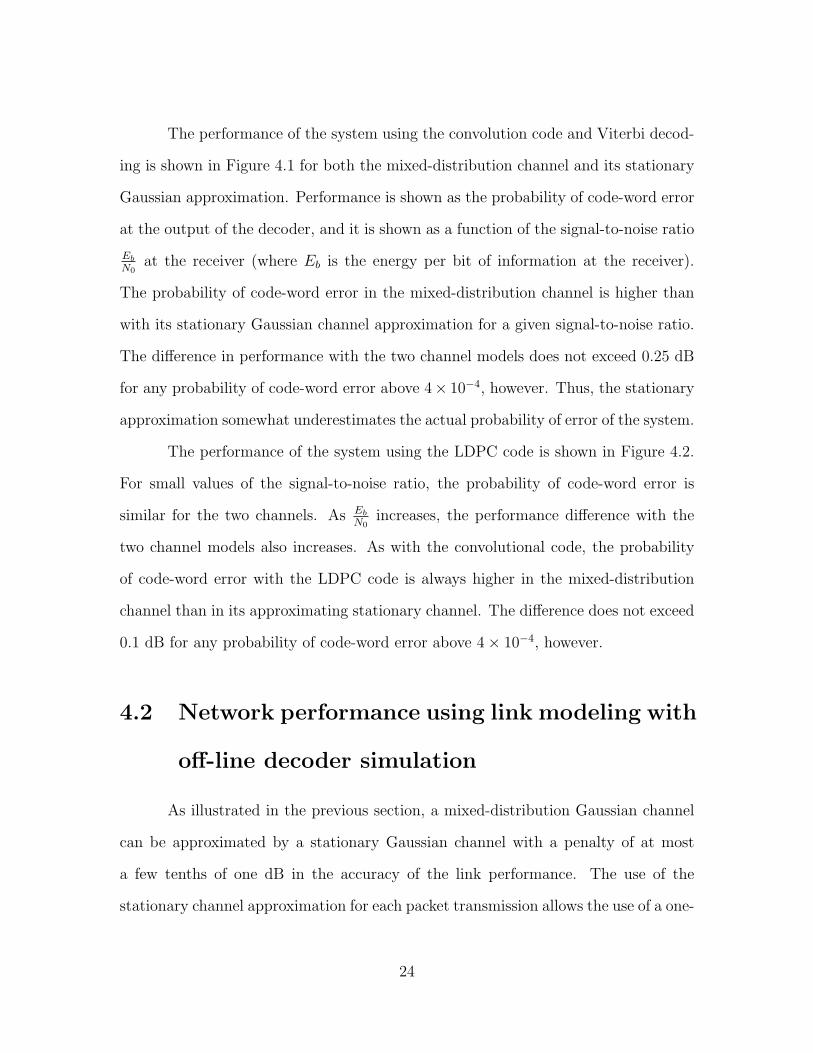
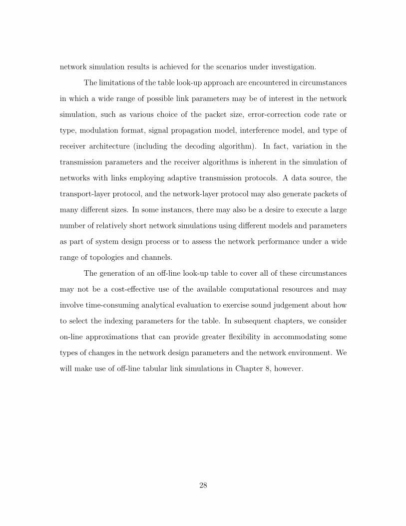
The performance of the system using the convolution code and Viterbi decod-
ing is shown in Figure 4.1 for both the mixed-distribution channel and its stationary
Gaussian approximation. Performance is shown as the probability of code-word error
at the output of the decoder, and it is shown as a function of the signal-to-noise ratio
Eb
N0at the receiver (where Eb is the energy per bit of information at the receiver).
The probability of code-word error in the mixed-distribution channel is higher than
with its stationary Gaussian channel approximation for a given signal-to-noise ratio.
The difference in performance with the two channel models does not exceed 0.25 dB
for any probability of code-word error above 4× 10⁻⁴, however. Thus, the stationary
approximation somewhat underestimates the actual probability of error of the system.
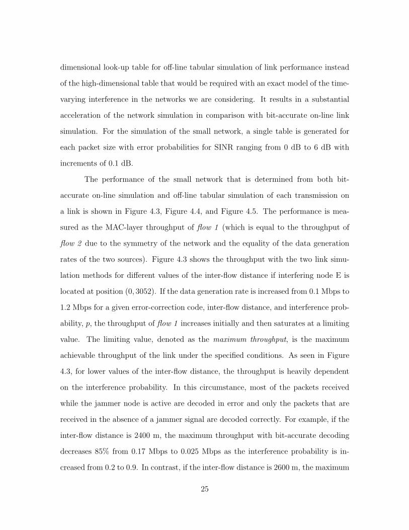
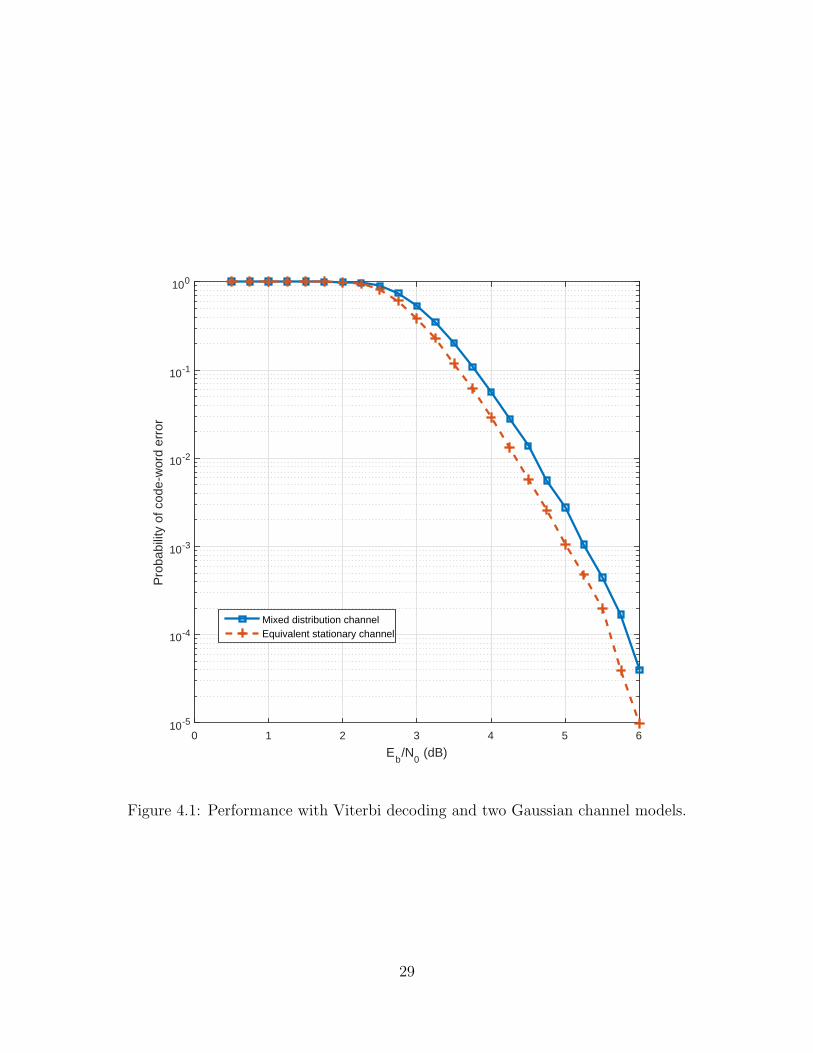
The performance of the system using the LDPC code is shown in Figure 4.2.
For small values of the signal-to-noise ratio, the probability of code-word error is
similar for the two channels. As Eb
N0increases, the performance difference with the
two channel models also increases. As with the convolutional code, the probability
of code-word error with the LDPC code is always higher in the mixed-distribution
channel than in its approximating stationary channel. The difference does not exceed
0.1 dB for any probability of code-word error above 4× 10⁻⁴, however.
4.2 Network performance using link modeling with
off-line decoder simulation
As illustrated in the previous section, a mixed-distribution Gaussian channel
can be approximated by a stationary Gaussian channel with a penalty of at most
a few tenths of one dB in the accuracy of the link performance. The use of the
stationary channel approximation for each packet transmission allows the use of a one-
24
dimensional look-up table for off-line tabular simulation of link performance instead
of the high-dimensional table that would be required with an exact model of the time-
varying interference in the networks we are considering. It results in a substantial
acceleration of the network simulation in comparison with bit-accurate on-line link
simulation. For the simulation of the small network, a single table is generated for
each packet size with error probabilities for SINR ranging from 0 dB to 6 dB with
increments of 0.1 dB.
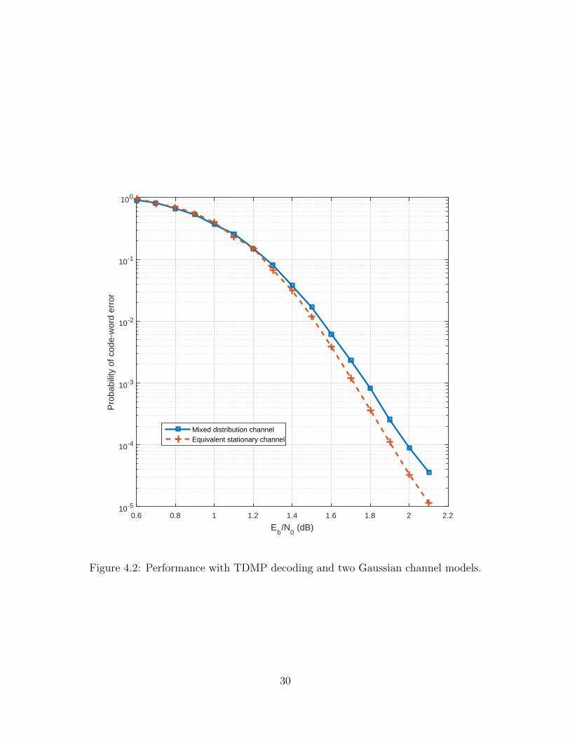
The performance of the small network that is determined from both bit-
accurate on-line simulation and off-line tabular simulation of each transmission on
a link is shown in Figure 4.3, Figure 4.4, and Figure 4.5. The performance is mea-
sured as the MAC-layer throughput of flow 1 (which is equal to the throughput of
flow 2 due to the symmetry of the network and the equality of the data generation
rates of the two sources). Figure 4.3 shows the throughput with the two link simu-
lation methods for different values of the inter-flow distance if interfering node E is
located at position (0, 3052). If the data generation rate is increased from 0.1 Mbps to
1.2 Mbps for a given error-correction code, inter-flow distance, and interference prob-
ability, p, the throughput of flow 1 increases initially and then saturates at a limiting
value. The limiting value, denoted as the maximum throughput, is the maximum
achievable throughput of the link under the specified conditions. As seen in Figure
4.3, for lower values of the inter-flow distance, the throughput is heavily dependent
on the interference probability. In this circumstance, most of the packets received
while the jammer node is active are decoded in error and only the packets that are
received in the absence of a jammer signal are decoded correctly. For example, if the
inter-flow distance is 2400 m, the maximum throughput with bit-accurate decoding
decreases 85% from 0.17 Mbps to 0.025 Mbps as the interference probability is in-
creased from 0.2 to 0.9. In contrast, if the inter-flow distance is 2600 m, the maximum
25
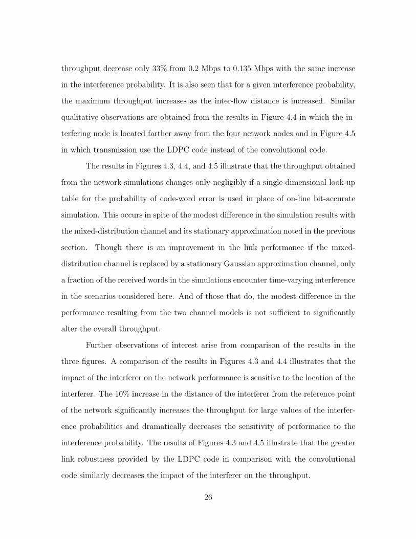
throughput decrease only 33% from 0.2 Mbps to 0.135 Mbps with the same increase
in the interference probability. It is also seen that for a given interference probability,
the maximum throughput increases as the inter-flow distance is increased. Similar
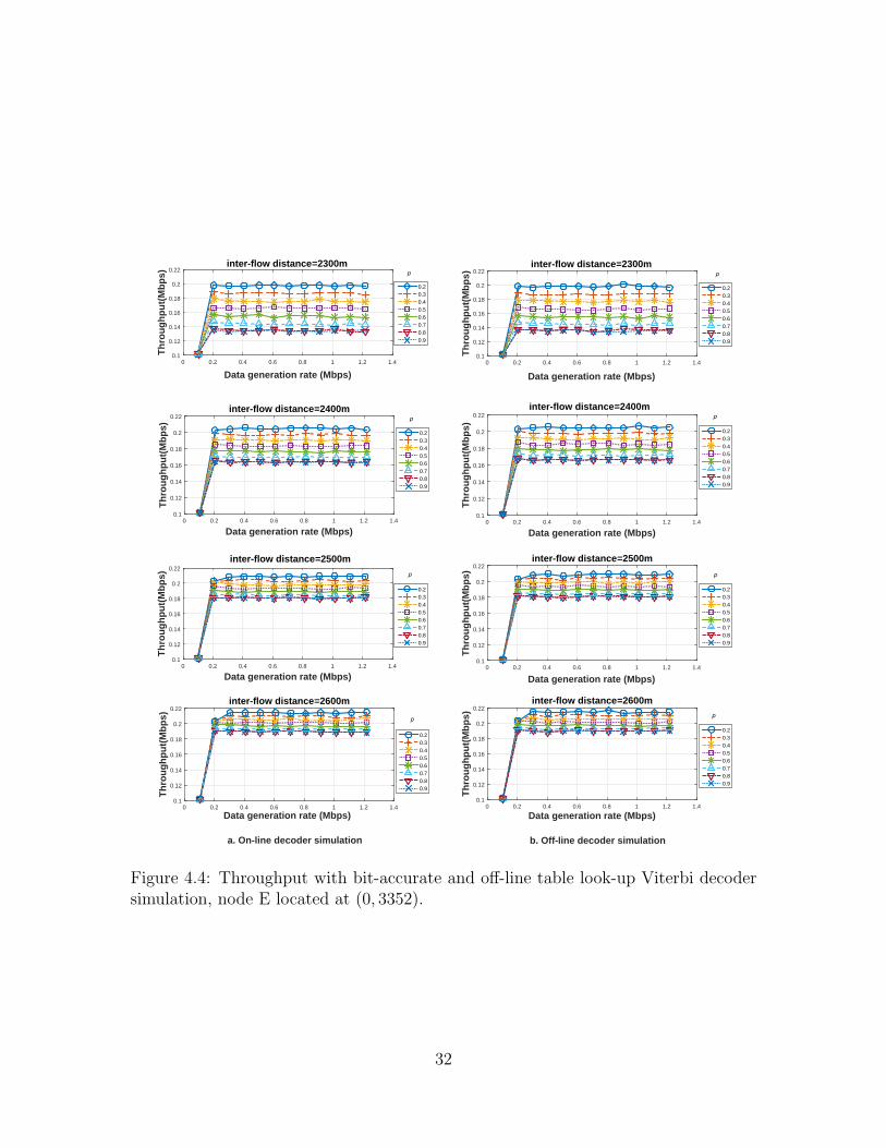
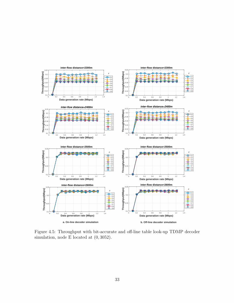
qualitative observations are obtained from the results in Figure 4.4 in which the in-
terfering node is located farther away from the four network nodes and in Figure 4.5
in which transmission use the LDPC code instead of the convolutional code.
The results in Figures 4.3, 4.4, and 4.5 illustrate that the throughput obtained
from the network simulations changes only negligibly if a single-dimensional look-up
table for the probability of code-word error is used in place of on-line bit-accurate
simulation. This occurs in spite of the modest difference in the simulation results with
the mixed-distribution channel and its stationary approximation noted in the previous
section. Though there is an improvement in the link performance if the mixed-
distribution channel is replaced by a stationary Gaussian approximation channel, only
a fraction of the received words in the simulations encounter time-varying interference
in the scenarios considered here. And of those that do, the modest difference in the
performance resulting from the two channel models is not sufficient to significantly
alter the overall throughput.
Further observations of interest arise from comparison of the results in the
three figures. A comparison of the results in Figures 4.3 and 4.4 illustrates that the
impact of the interferer on the network performance is sensitive to the location of the
interferer. The 10% increase in the distance of the interferer from the reference point
of the network significantly increases the throughput for large values of the interfer-
ence probabilities and dramatically decreases the sensitivity of performance to the
interference probability. The results of Figures 4.3 and 4.5 illustrate that the greater
link robustness provided by the LDPC code in comparison with the convolutional
code similarly decreases the impact of the interferer on the throughput.
26
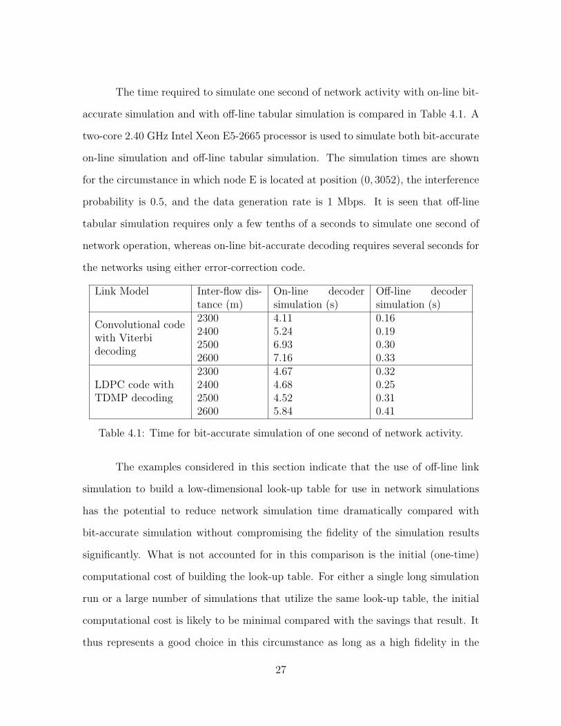
The time required to simulate one second of network activity with on-line bit-
accurate simulation and with off-line tabular simulation is compared in Table 4.1. A
two-core 2.40 GHz Intel Xeon E5-2665 processor is used to simulate both bit-accurate
on-line simulation and off-line tabular simulation. The simulation times are shown
for the circumstance in which node E is located at position (0, 3052), the interference
probability is 0.5, and the data generation rate is 1 Mbps. It is seen that off-line
tabular simulation requires only a few tenths of a seconds to simulate one second of
network operation, whereas on-line bit-accurate decoding requires several seconds for
the networks using either error-correction code.
Link Model Inter-flow dis-tance (m)
On-line decodersimulation (s)
Off-line decodersimulation (s)
Convolutional codewith Viterbidecoding
2300 4.11 0.162400 5.24 0.192500 6.93 0.302600 7.16 0.33
LDPC code withTDMP decoding
2300 4.67 0.322400 4.68 0.252500 4.52 0.312600 5.84 0.41
Table 4.1: Time for bit-accurate simulation of one second of network activity.
The examples considered in this section indicate that the use of off-line link
simulation to build a low-dimensional look-up table for use in network simulations
has the potential to reduce network simulation time dramatically compared with
bit-accurate simulation without compromising the fidelity of the simulation results
significantly. What is not accounted for in this comparison is the initial (one-time)
computational cost of building the look-up table. For either a single long simulation
run or a large number of simulations that utilize the same look-up table, the initial
computational cost is likely to be minimal compared with the savings that result. It
thus represents a good choice in this circumstance as long as a high fidelity in the
27
network simulation results is achieved for the scenarios under investigation.
The limitations of the table look-up approach are encountered in circumstances
in which a wide range of possible link parameters may be of interest in the network
simulation, such as various choice of the packet size, error-correction code rate or
type, modulation format, signal propagation model, interference model, and type of
receiver architecture (including the decoding algorithm). In fact, variation in the
transmission parameters and the receiver algorithms is inherent in the simulation of
networks with links employing adaptive transmission protocols. A data source, the
transport-layer protocol, and the network-layer protocol may also generate packets of
many different sizes. In some instances, there may also be a desire to execute a large
number of relatively short network simulations using different models and parameters
as part of system design process or to assess the network performance under a wide
range of topologies and channels.
The generation of an off-line look-up table to cover all of these circumstances
may not be a cost-effective use of the available computational resources and may
involve time-consuming analytical evaluation to exercise sound judgement about how
to select the indexing parameters for the table. In subsequent chapters, we consider
on-line approximations that can provide greater flexibility in accommodating some
types of changes in the network design parameters and the network environment. We
will make use of off-line tabular link simulations in Chapter 8, however.
28
Eb/N
0 (dB)
0 1 2 3 4 5 6
Pro
babi
lity
of c
ode-
wor
d er
ror
10-5
10-4
10-3
10-2
10-1
100
Mixed distribution channelEquivalent stationary channel
Figure 4.1: Performance with Viterbi decoding and two Gaussian channel models.
29
Eb/N
0 (dB)
0.6 0.8 1 1.2 1.4 1.6 1.8 2 2.2
Pro
babi
lity
of c
ode-
wor
d er
ror
10-5
10-4
10-3
10-2
10-1
100
Mixed distribution channelEquivalent stationary channel
Figure 4.2: Performance with TDMP decoding and two Gaussian channel models.
30
Data generation rate(Mbps)0 0.2 0.4 0.6 0.8 1 1.2 1.4
Th
rou
gh
pu
t(M
bp
s)
0
0.05
0.1
0.15
0.2inter-flow distance=2300m
0.2
0.3
0.4
0.5
0.6
0.7
0.8
0.9
Data generation rate(Mbps)0 0.2 0.4 0.6 0.8 1 1.2 1.4
Th
rou
gh
pu
t(M
bp
s)
0
0.05
0.1
0.15
0.2inter-flow distance=2300m
0.2
0.3
0.4
0.5
0.6
0.7
0.8
0.9
Data generation rate(Mbps)
0 0.2 0.4 0.6 0.8 1 1.2 1.4
Th
rou
gh
pu
t(M
bp
s)
0
0.05
0.1
0.15
0.2inter-flow distance=2400m
0.2
0.3
0.4
0.5
0.6
0.7
0.8
0.9
Data generation rate(Mbps)
0 0.2 0.4 0.6 0.8 1 1.2 1.4
Th
rou
gh
pu
t(M
bp
s)
0
0.05
0.1
0.15
0.2inter-flow distance=2400m
0.2
0.3
0.4
0.5
0.6
0.7
0.8
0.9
p p
pp
Data generation rate (Mbps)0 0.2 0.4 0.6 0.8 1 1.2 1.4
Th
rou
gh
pu
t(M
bp
s)
0
0.05
0.1
0.15
0.2inter-flow distance=2500m
0.20.30.40.50.60.70.80.9
Data generation rate (Mbps)
b. Off-line decoder simulation
0 0.2 0.4 0.6 0.8 1 1.2 1.4
Th
rou
gh
pu
t(M
bp
s)
0
0.05
0.1
0.15
0.2
0.25inter-flow distance=2600m
0.20.30.40.50.60.70.80.9
Data generation rate (Mbps)0 0.2 0.4 0.6 0.8 1 1.2 1.4
Th
rou
gh
pu
t(M
bp
s)
0
0.05
0.1
0.15
0.2inter-flow distance=2500m
0.20.30.40.50.60.70.80.9
Data generation rate (Mbps)
a. On-line decoder simulation
0 0.2 0.4 0.6 0.8 1 1.2 1.4
Th
rou
gh
pu
t(M
bp
s)
0
0.05
0.1
0.15
0.2
0.25inter-flow distance=2600m
0.20.30.40.50.60.70.80.9
p
p
p
p
Figure 4.3: Throughput with bit-accurate and off-line table look-up Viterbi decodersimulation, node E located at (0, 3052).
31
Data generation rate (Mbps)0 0.2 0.4 0.6 0.8 1 1.2 1.4
Th
rou
gh
pu
t(M
bp
s)
0.1
0.12
0.14
0.16
0.18
0.2
0.22inter-flow distance=2300m
0.20.30.40.50.60.70.80.9
Data generation rate (Mbps)
0 0.2 0.4 0.6 0.8 1 1.2 1.4
Th
rou
gh
pu
t(M
bp
s)
0.1
0.12
0.14
0.16
0.18
0.2
0.22inter-flow distance=2300m
0.20.30.40.50.60.70.80.9
Data generation rate (Mbps)0 0.2 0.4 0.6 0.8 1 1.2 1.4
Th
rou
gh
pu
t(M
bp
s)
0.1
0.12
0.14
0.16
0.18
0.2
0.22inter-flow distance=2400m
0.20.30.40.50.60.70.80.9
Data generation rate (Mbps)0 0.2 0.4 0.6 0.8 1 1.2 1.4
Th
rou
gh
pu
t(M
bp
s)
0.1
0.12
0.14
0.16
0.18
0.2
0.22inter-flow distance=2400m
0.20.30.40.50.60.70.80.9
p
p p
p
Data generation rate (Mbps)0 0.2 0.4 0.6 0.8 1 1.2 1.4
Th
rou
gh
pu
t(M
bp
s)
0.1
0.12
0.14
0.16
0.18
0.2
0.22inter-flow distance=2500m
0.20.30.40.50.60.70.80.9
Data generation rate (Mbps)
b. Off-line decoder simulation
0 0.2 0.4 0.6 0.8 1 1.2 1.4
Th
rou
gh
pu
t(M
bp
s)
0.1
0.12
0.14
0.16
0.18
0.2
0.22inter-flow distance=2600m
0.20.30.40.50.60.70.80.9
Data generation rate (Mbps)0 0.2 0.4 0.6 0.8 1 1.2 1.4
Th
rou
gh
pu
t(M
bp
s)
0.1
0.12
0.14
0.16
0.18
0.2
0.22inter-flow distance=2500m
0.20.30.40.50.60.70.80.9
Data generation rate (Mbps)
a. On-line decoder simulation
0 0.2 0.4 0.6 0.8 1 1.2 1.4
Th
rou
gh
pu
t(M
bp
s)
0.1
0.12
0.14
0.16
0.18
0.2
0.22inter-flow distance=2600m
0.20.30.40.50.60.70.80.9
p
pp
p
Figure 4.4: Throughput with bit-accurate and off-line table look-up Viterbi decodersimulation, node E located at (0, 3352).
32
Data generation rate (Mbps)0 0.2 0.4 0.6 0.8 1 1.2 1.4
Th
rou
gh
pu
t(M
bp
s)
0.1
0.12
0.14
0.16
0.18
0.2
0.22 inter-flow distance=2300m
0.20.30.40.50.60.70.80.9
Data generation rate (Mbps)0 0.2 0.4 0.6 0.8 1 1.2 1.4
Th
rou
gh
pu
t(M
bp
s)
0.1
0.12
0.14
0.16
0.18
0.2
0.22inter-flow distance=2300m
0.20.30.40.50.60.70.80.9
Data generation rate (Mbps)0 0.2 0.4 0.6 0.8 1 1.2 1.4
Th
rou
gh
pu
t(M
bp
s)
0.1
0.12
0.14
0.16
0.18
0.2
0.22inter-flow distance=2400m
0.20.30.40.50.60.70.80.9
Data generation rate (Mbps)0 0.2 0.4 0.6 0.8 1 1.2 1.4
Th
rou
gh
pu
t(M
bp
s)
0.1
0.12
0.14
0.16
0.18
0.2
0.22inter-flow distance=2400m
0.20.30.40.50.60.70.80.9
p
pp
p
Data generation rate (Mbps)0 0.2 0.4 0.6 0.8 1 1.2 1.4
Th
rou
gh
pu
t(M
bp
s)
0.1
0.15
0.2
0.25inter-flow distance=2500m
0.20.30.40.50.60.70.80.9
Data generation rate (Mbps)0 0.2 0.4 0.6 0.8 1 1.2 1.4
Th
rou
gh
pu
t(M
bp
s)
0.1
0.15
0.2
0.25inter-flow distance=2500m
0.20.30.40.50.60.70.80.9
Data generation rate (Mbps)
a. On-line decoder simulation
0 0.2 0.4 0.6 0.8 1 1.2 1.4
Th
rou
gh
pu
t(M
bp
s)
0.1
0.15
0.2
0.25inter-flow distance=2600m
0.20.30.40.50.60.70.80.9
Data generation rate (Mbps)
b. Off-line decoder simulation
0 0.2 0.4 0.6 0.8 1 1.2 1.4
Th
rou
gh
pu
t(M
bp
s)
0.1
0.15
0.2
0.25inter-flow distance=2600m
0.20.30.40.50.60.70.80.9
p p
p
p
Figure 4.5: Throughput with bit-accurate and off-line table look-up TDMP decodersimulation, node E located at (0, 3052).
33
Chapter 5
Approximations in On-Line Viterbi
Decoder Simulation
Several closed-form expressions for an upper bound on the probability of code-
word error at the output of a Viterbi decoder have been developed for a system using
convolutional coding and binary antipodal modulation (such as BPSK modulation).
In this chapter, the tightest two such upper bounds from the literature are consid-
ered as approximations that are used in on-line determination of link transmission
outcomes in a network simulation. The closed-form expression for each bound is
evaluated with modest computation for each transmission and is applicable to an ar-
bitrary convolutional code and packet length without the need for significant on-line
storage. Approximation of link transmission outcomes based on an SINR threshold
is also considered.
34
5.1 Closed-form approximations to the probability
of code-word error
Numerous closed-form bounds have been developed for the probability of code-
word error for convolutional coding with Viterbi decoding over an additive white
Gaussian noise channel [14]. The two tightest bounds to date for a receiver using
soft-decision Viterbi decoding are the tighter concave-Chernoff bound and the concave
integral bound [14]. The tighter concave-Chernoff bound for code word of block length
L is given by
Pe ≤ 1− (1− Pt−ch)L (5.1)
where
Pt−ch = Q
(√2dfreeEc
N0
)exp
(dfreeEc
N0
)T (W )
∣∣∣∣W=exp
(−Ec
N0
) .Here, dfree is the minimum free Hamming distance of the code, Ec is the energy
per channel symbol, N0 is the noise power spectral density, and T (W ) is the path
enumerator of the code [44].
Similarly the concave integral bound for the code can be expressed in terms
of the first-event union bound Pu as
Pe ≤ 1− (1− Pu)L (5.2)
where
Pu =1
π
∫ π2
0
T (W )|W=exp
(− Ec
N0sin2θ
) dθ.Application of the bounds in Equations ( 5.1) and ( 5.2) requires knowledge
of the path enumerator and the minimum free Hamming distance of the code. For
35
System Link model1 bit-accurate soft-decision Viterbi decoder2 tighter concave-Chernoff bound3 concave-integral bound4 SINR threshold
Table 5.1: Link models for simulation systems considered.
the NASA-standard convolutional code used in the examples, T (W ) is given in [47]
and the minimum free Hamming distance is dfree = 10. Either bound is applied in
the network simulation by first approximating the mixed-distribution by the equiv-
alent stationary Gaussian channel and then using the noise power spectral density
of the equivalent stationary channel in the expression for the bound. For each link
transmission outcome, the value of the bound is determined and used to generate an
outcome of a correspondingly weighted Bernoulli random variable.
5.2 Threshold-based approximation to the proba-
bility of code-word error
The threshold-based approximation utilizes the SINR at the receiver based on
the noise power spectral density of the equivalent Gaussian channel. For each link
transmission outcome, the SINR is compared against a preset threshold. If the SINR
exceeds the threshold, the transmission is modeled as successful in the simulation.
Otherwise, it is modeled as a failure. The threshold is determined by running the
network simulation for different threshold values and choosing the value that produces
results closest to the online bit-accurate simulations.
36
5.3 Comparison of simulation results
The performance of the small network is simulated using bit-accurate link
simulation and each of the three approximations described in the previous sections.
The models using the different link models are denoted as Systems 1, 2, 3, and 4.
System 1 denotes the simulation using the bit-accurate soft-decision Viterbi decoding.
System 2 and System 3 denote the simulations using the tighter concave-Chernoff
bound and concave-integral bound link approximations, respectively. And System 4
denotes the simulation employing the SINR threshold link approximation. (The SINR
threshold for System 4 is 3.2 dB in the examples.) Table 5.1 lists the four systems.
Figure 5.1 shows the throughput of flow 1 in the small network as a function of
the data generation rate in simulation Systems 1 to 4 if node E is located at position
(0, 3052). The throughput is shown for different values of the inter-flow distance and
two values of the interference probability, p = 0.2 and p = 0.9. For each system,
the throughput increases with either an increasing inter-flow distance or a decreasing
interference probability as is consistent with a reasonable link model.
The throughput is essentially the same in each system if the inter-flow distance
is either small or large. If the inter-flow distance is 3000 m or greater, interfering
signals from the jammer and the other network nodes are very weak at each receiver,
resulting in a large SINR at the receiver even in the presence of interference. Channel-
access contention between the two flows is moderate, and data transmissions are
successful with a fairly high probability even in the presence of the jamming signal.
Both closed-formed bounds yield an accurate approximation to the probability of
code-word error with a high SINR and thus Systems 2 and 3 yield a similar throughput
to System 1. A properly tuned SINR threshold also yields similar results with System
4.
37
If the inter-flow distance is only 2300 m, in contrast, the interference probabil-
ity has a dramatic effect on the maximum throughput in each system. The maximum
throughput is limited by the significant channel-access contention between the two
flows if the interference probability is small, and it is limited by the strong jammer
signal if the interference probability is large. Most successful data packet transmis-
sions occur only if the jammer is inactive in which case the SINR at the receiver is
large, in which circumstance the link models yield similar results. Thus the through-
put for all four systems is similar if p = 0.2. If p = 0.9, the interference precludes
significant throughput in all four systems.
If the inter-flow distance is intermediate between 2300 m and 3000 m, however,
greater variability among the four simulation systems is observed. A data transmis-
sion occurring in the presence of jammer interference in this range of distances results
in an SINR at the receiver which is large enough to result in successful transmission
with a non-negligible probability but small enough that the two bounds substan-
tially overestimate the probability of code-word error. Consequently, the maximum
throughput determined by simulation Systems 2 and 3 is slightly lower than the
throughput determined by System 1 if the interference probability is small, and it is
much lower if the interference probability is large. If p = 0.9 and the inter-flow dis-
tance is 2400 m, the maximum throughput of System 1 is 0.025 Mbps, but the bounds
used in Systems 2 and 3 result in negligible throughput. If instead the inter-flow dis-
tance is 2500 m, the maximum throughput of System 3 is approximately one-half that
of System 1, and the maximum throughput of System 2 is even less. For larger values
of the inter-flow distance, the difference in the maximum throughput among Systems
1, 2, and 3 decreases considerably, as seen for example if the inter-flow distance is
2700 m.
In each circumstance shown in Figure 5.1, simulation Systems 2 and 3 approx-
38
imate the performance of the bit-accurate simulation System 1 more closely than does
System 4 (which uses the SINR threshold). For inter-flow distances up 2500 m, Sys-
tem 4 underestimates the network performance more severely than does either System
2 or System 3. For inter-flow distances of 2600 m and above, System 4 overestimates
the network performance, most severely if the interference probability is large. For
example, it overestimates the performance by 30% if the inter-flow distance is 2600
m and p = 0.9.
Similar observations arise from Figure 5.2 which shows the performance of the
four simulation systems under the same circumstances as in Figure 5.1 except that
node E is located farther away at position (0, 3352). If the inter-flow distance is either
small or large, Systems 2, 3 and 4 yield results similar to those of System 1. But for
intermediate values of the inter-flow distance, the maximum throughput of System 2
and System 3 matches the maximum throughput of System 1 more closely than does
the maximum throughput of System 4. The mismatch of results from System 4 is
pronounced for these values of the inter-flow distance if the interference probability
is large.
Table 5.2 shows the time required to simulate 1s of network activity using a
2 core 2.70 GHz Intel Xeon E5-2680 processor for simulation of Systems 1-4 if the
inter-flow distance is 2400m and the data generation rate is 1 Mbps. Simulation times
are shown for interference probabilities of 0.2 and 0.9 and with the interfering node
in either of the two locations considered above. It is observed that for a given link
model, the simulation time increases as the throughput increases. Bit-accurate Viterbi
decoding involves numerous calculations that increase the simulation time of System 1
by several-fold compared with Systems 2-4. The evaluation of an integral function in
the concave-integral bound results in System 3 exhibiting the next greatest simulation
time. System 2 and 4 have the smallest simulation times because they require only
39
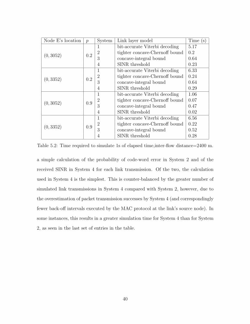
Node E’s location p System Link layer model Time (s)
(0, 3052) 0.2
1 bit-accurate Viterbi decoding 5.172 tighter concave-Chernoff bound 0.23 concave-integral bound 0.644 SINR threshold 0.23
(0, 3352) 0.2
1 bit-accurate Viterbi decoding 6.332 tighter concave-Chernoff bound 0.243 concave-integral bound 0.644 SINR threshold 0.29
(0, 3052) 0.9
1 bit-accurate Viterbi decoding 1.062 tighter concave-Chernoff bound 0.073 concave-integral bound 0.474 SINR threshold 0.02
(0, 3352) 0.9
1 bit-accurate Viterbi decoding 6.562 tighter concave-Chernoff bound 0.223 concave-integral bound 0.524 SINR threshold 0.28
Table 5.2: Time required to simulate 1s of elapsed time,inter-flow distance=2400 m.
a simple calculation of the probability of code-word error in System 2 and of the
received SINR in System 4 for each link transmission. Of the two, the calculation
used in System 4 is the simplest. This is counter-balanced by the greater number of
simulated link transmissions in System 4 compared with System 2, however, due to
the overestimation of packet transmission successes by System 4 (and correspondingly
fewer back-off intervals executed by the MAC protocol at the link’s source node). In
some instances, this results in a greater simulation time for System 4 than for System
2, as seen in the last set of entries in the table.
40
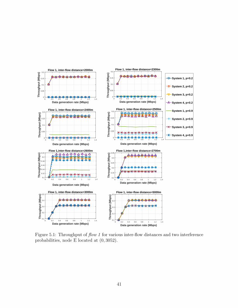
Data generation rate (Mbps)0 0.2 0.4 0.6 0.8 1 1.2 1.4
Th
rou
gh
pu
t (M
bp
s)
0
0.05
0.1
0.15
0.2Flow 1, inter-flow distance=2000m
Data generation rate (Mbps)0 0.2 0.4 0.6 0.8 1 1.2 1.4
Th
rou
gh
pu
t (M
bp
s)
0
0.05
0.1
0.15
0.2Flow 1, inter-flow distance=2300m
System 1, p=0.2
System 2, p=0.2
System 3, p=0.2
System 4, p=0.2
System 1, p=0.9
System 2, p=0.9
System 3, p=0.9
System 4, p=0.9
Data generation rate (Mbps)
0 0.2 0.4 0.6 0.8 1 1.2 1.4
Th
rou
gh
pu
t (M
bp
s)
0
0.05
0.1
0.15
0.2Flow 1, inter-flow distance=2500m
Data generation rate (Mbps)
0 0.2 0.4 0.6 0.8 1 1.2 1.4
Th
rou
gh
pu
t (M
bp
s)
0
0.05
0.1
0.15
0.2Flow 1, inter-flow distance=2400m
Data generation rate (Mbps)
0 0.2 0.4 0.6 0.8 1 1.2 1.4
Th
rou
gh
pu
t (M
bp
s)
0.1
0.12
0.14
0.16
0.18
0.2
0.22Flow 1,inter-flow distance=2600m
Data generation rate (Mbps)0 0.2 0.4 0.6 0.8 1 1.2 1.4
Th
rou
gh
pu
t (M
bp
s)
0.1
0.2
0.3
0.4
0.5Flow 1, inter-flow distance=3000m
Data generation rate (Mbps)0 0.2 0.4 0.6 0.8 1 1.2 1.4
Th
rou
gh
pu
t (M
bp
s)
0.1
0.15
0.2
0.25
0.3
0.35Flow 1,inter-flow distance=2700m
Data generation rate (Mbps)0 0.2 0.4 0.6 0.8 1 1.2 1.4
Th
rou
gh
pu
t (M
bp
s)
0.1
0.2
0.3
0.4
0.5Flow 1, inter-flow distance=5000m
Figure 5.1: Throughput of flow 1 for various inter-flow distances and two interferenceprobabilities, node E located at (0, 3052).
41
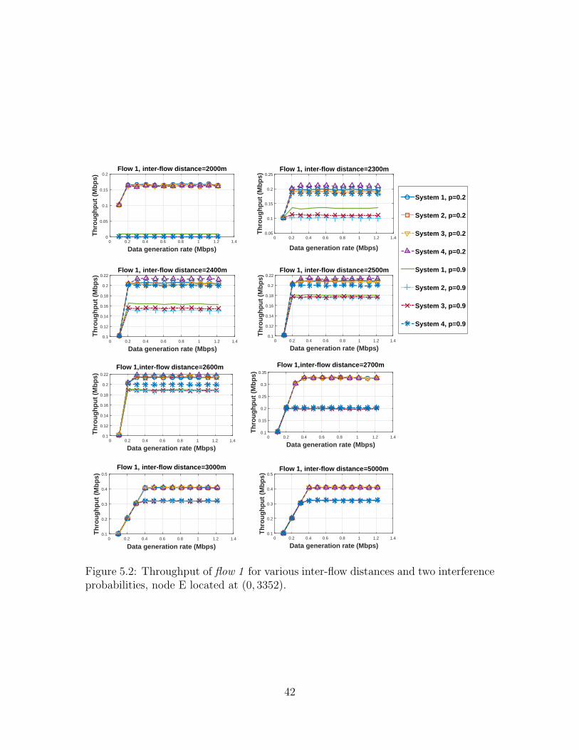
Data generation rate (Mbps)0 0.2 0.4 0.6 0.8 1 1.2 1.4
Th
rou
gh
pu
t (M
bp
s)
0
0.05
0.1
0.15
0.2Flow 1, inter-flow distance=2000m
Data generation rate (Mbps)
0 0.2 0.4 0.6 0.8 1 1.2 1.4
Th
rou
gh
pu
t (M
bp
s)
0.05
0.1
0.15
0.2
0.25Flow 1, inter-flow distance=2300m
System 1, p=0.2
System 2, p=0.2
System 3, p=0.2
System 4, p=0.2
System 1, p=0.9
System 2, p=0.9
System 3, p=0.9
System 4, p=0.9
Data generation rate (Mbps)0 0.2 0.4 0.6 0.8 1 1.2 1.4
Th
rou
gh
pu
t (M
bp
s)
0.1
0.12
0.14
0.16
0.18
0.2
0.22Flow 1, inter-flow distance=2500m
Data generation rate (Mbps)0 0.2 0.4 0.6 0.8 1 1.2 1.4
Th
rou
gh
pu
t (M
bp
s)
0.1
0.12
0.14
0.16
0.18
0.2
0.22Flow 1, inter-flow distance=2400m
Data generation rate (Mbps)0 0.2 0.4 0.6 0.8 1 1.2 1.4
Th
rou
gh
pu
t (M
bp
s)
0.1
0.12
0.14
0.16
0.18
0.2
0.22
Flow 1,inter-flow distance=2600m
Data generation rate (Mbps)0 0.2 0.4 0.6 0.8 1 1.2 1.4
Th
rou
gh
pu
t (M
bp
s)
0.1
0.2
0.3
0.4
0.5
Flow 1, inter-flow distance=3000m
Data generation rate (Mbps)0 0.2 0.4 0.6 0.8 1 1.2 1.4
Th
rou
gh
pu
t (M
bp
s)
0.1
0.15
0.2
0.25
0.3
0.35
Flow 1,inter-flow distance=2700m
Data generation rate (Mbps)0 0.2 0.4 0.6 0.8 1 1.2 1.4
Th
rou
gh
pu
t (M
bp
s)
0.1
0.2
0.3
0.4
0.5Flow 1, inter-flow distance=5000m
Figure 5.2: Throughput of flow 1 for various inter-flow distances and two interferenceprobabilities, node E located at (0, 3352).
42
Chapter 6
GPU-Accelerated On-Line Viterbi
Decoder Simulation
It is apparent from the results in the previous chapter that simulation of
the performance of an ad hoc radio network requires computation time that can be
dominated by the implementation of the error-correction decoder in the receiver if
bit-accurate modeling of each link transmission is employed. Simplified models of
the outcomes of link transmissions using either a closed-form analytical expression
or a threshold test to approximate the link performance can significantly reduce the
simulation time, albeit with some loss in the fidelity of the simulated network perfor-
mance. An alternative approach to reducing the network simulation time is to employ
“accelerator” hardware for bit-accurate implementation of the decoding.
Options for acceleration include a graphical processor unit (GPU), a field-
programmable gate array, or any of numerous other specialized computing archi-
tectures that support a high level of cost-effective parallelism for an appropriately
structured task. A GPU has an architecture that is designed to efficiently support
large-scale parallelism on arithmetically intensive tasks that exhibit high data-level
43
parallelism and thread-level parallelism with thread-specific branching decisions that
are rare or non-existent and infrequent, highly structured memory access. Many com-
putationally intensive algorithms of digital communications are well matched to the
GPU architecture; among these are many decoding algorithms for error-correction
codes, including Viterbi decoding of convolutional codes, turbo decoding of parallel
concatenated convolutional codes (turbo codes), and the various belief-propagation
decoding algorithms (such as the TDMP algorithm) for LDPC codes.
In this and subsequent chapters, we consider the use of a GPU as an acceler-
ator for a network simulation. In this chapter, we focus on its use to implement the
Viterbi decoder of the NASA-standard rate-1/2 convolutional code. A baseline im-
plementation of the decoder is considered, and two improvements are addressed. The
first improvement uses improved GPU memory management to reduce data-transfer
latencies, and the second one adapts the Viterbi decoder to better exploit the GPU
architecture.
6.1 Introduction to GPUs
In GPU-accelerated computing, a CPU transfers the arithmetically intensive
work to the GPU and retains the logic intensive parts of the program. Unlike a
CPU which has a small number of cores with a small number of threads sharing
the computation time of each core, a GPU has hundreds of cores with each core
capable of running hundreds of threads in parallel. The most widely used GPUs
are designed by NVIDIA, and the Compute Unified Device Architecture (CUDA)
[48] is a parallel computing platform and programing model that provides a high-
level interface for utilization of the resources in a NVIDIA GPU. It also facilitates
communication and efficient collaboration among programs executed in the CPU and
44
GPU. Our subsequent discussion of GPUs is in terms of the NVIDIA TESLA k40
GPU we use to obtain numerical results reported in the dissertation.
GPUs are well suited to executing the same instruction on multiple data el-
ements. To manage a large number of threads, it employs the Single-Instruction,
Multiple-Thread (SIMT) architecture. The SIMT architecture is very similar to
Single-Instruction, Multiple-Data architecture [49] as a single instruction controls
multiple arithmetic units in both architectures. The instructions in the SIMT ar-
chitecture also have the ability to specify the execution and behavior of individual
threads, however. This allows both thread-level parallel codes for independent threads
and data-level parallel codes for coordinated threads to be written for the SIMT ar-
chitecture. This flexibility proves very useful for implementing the Viterbi decoder
on a GPU.
The number of threads required to execute a segment of code in parallel is
specified when launching a kernel. The kernel is the part of the program that is to
be executed in the GPU. When a kernel is launched, it is executed on the streaming
multiprocessors (SMs) of the GPU. An SM is a collection of stream processors (SPs)
[50], also called “CUDA cores”. The blocks of thread assigned for a program are
divided equally among the SMs and each SM executes the blocks of threads in groups
of 32 parallel threads called “warps”. The total number of threads executed in parallel
depends on the number of SMs in the GPU and the number of warps executed per
SM. At the least, all the threads in a block are executed in parallel by the SM.
Memory management is another critical factor in GPU computation. The
data required by the kernel must be transferred from off-chip memory onto the GPU
before the kernel is executed, and data results must be transferred from the GPU
memory to the off-chip memory after execution of the kernel has terminated. This
data transfer has a large overhead compared to the processing times in the GPU, and
45
the transfer time increases linearly with the amount of data that must be transferred.
An understanding of the GPU architecture and the memory architecture allows the
user to optimize program execution and data management in the GPU.
6.2 Memory organization in the GPU
Data transfer to and from the GPU memory is a bottleneck in GPU program
execution. Consequently, optimal memory management is very important to overall
execution time of the program on the GPU [48], and a knowledge of the memory
organization aides in efficient use of available memory resources. Figure 6.1 shows
the memory organization on a GPU. There are five types of memory: registers, local
memory, shared memory, global memory, and constant memory.
Registers are located on the GPU chip, and data in a register is accessed more
rapidly by the GPU than data in any of the other types of memory. Automatic
variables [51] are stored in registers. Each thread has exclusive access to its allocated
registers. Automatic variables such as arrays and structures that are too large for the
registers are stored in local memory. Local memory is so named because of its scope,
not because of its location. Only a single thread can access a given local memory
during execution of the kernel. Since it is located off-chip, access of local memory by
the GPU is slow.
Data that must be available to multiple threads is stored in either shared
memory or global memory. Shared memory is located on-chip; hence, access to it by
the GPU is fast. All threads belonging to a single block can access data in the shared
memory assigned to the block. Since shared memory is located on-chip, however, it
is limited and should be used for small data arrays.
Global memory is the largest memory available, but it is located off-chip and
46
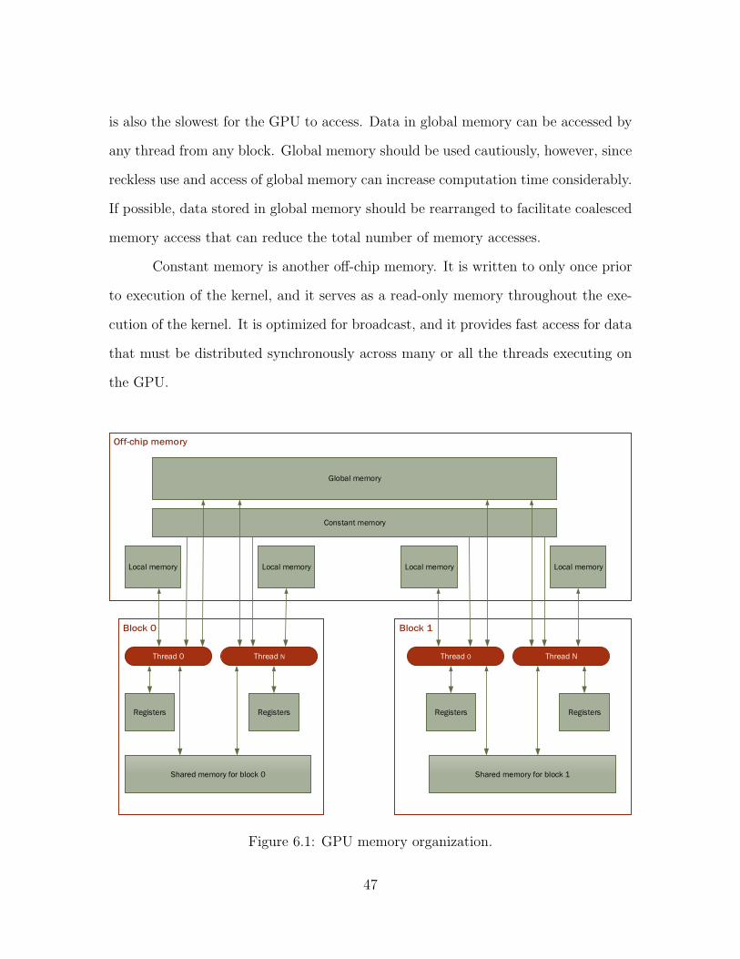
is also the slowest for the GPU to access. Data in global memory can be accessed by
any thread from any block. Global memory should be used cautiously, however, since
reckless use and access of global memory can increase computation time considerably.
If possible, data stored in global memory should be rearranged to facilitate coalesced
memory access that can reduce the total number of memory accesses.
Constant memory is another off-chip memory. It is written to only once prior
to execution of the kernel, and it serves as a read-only memory throughout the exe-
cution of the kernel. It is optimized for broadcast, and it provides fast access for data
that must be distributed synchronously across many or all the threads executing on
the GPU.
Global memory
Constant memory
Local memory Local memory Local memory Local memory
Thread 0 Thread N Thread 0 Thread N
Registers RegistersRegistersRegisters
Shared memory for block 0 Shared memory for block 1
Figure 6.1: GPU memory organization.
47
6.3 Parallel Viterbi decoding
The soft-decision Viterbi decoding algorithm [44] is a dynamic programming
algorithm used for decoding with convolutional codes. The algorithm acts upon the
labeled trellis structure generated by the temporal evolution of the convolutional en-
coder viewed as a finite-state machine. It searches for the path through the trellis
with a code-label sequence that is closest in Euclidean distance [44] to the received
word. The Viterbi algorithm is a maximum-likelihood decoder for many commu-
nication channels of interest (including the stationary Gaussian noise channel) and
so achieves the minimum probability of code-word error for a uniform information
source.
The execution of the Viterbi algorithm on a single received word can be divided
into two main phases: the forward pass, and the traceback. In the forward-pass phase,
a branch metric is calculated for each branch in the trellis based on its code-symbol
labels and the received symbols corresponding to the time step of the branch. The
sum of the branch metrics of the branches forming a path through the trellis form its
path metric, and the algorithm determines enough information about the path metric
for each path to determine the minimum-metric path through the trellis terminating
at each state in the trellis at the final time step. Because of the trellis structure, this is
accomplished efficiently by the algorithm moving sequentially through the time steps
represented by the trellis, calculating all branch metrics for a given time step at that
step and updating the partial information about path metrics obtained to that point
in time. As discussed in the next subsection, it is well-suited to parallelization of the
computation performed for a given time step, though the computation for different
time steps is inherently sequential.
The traceback phase traces the path that is closest to the received vector once
48
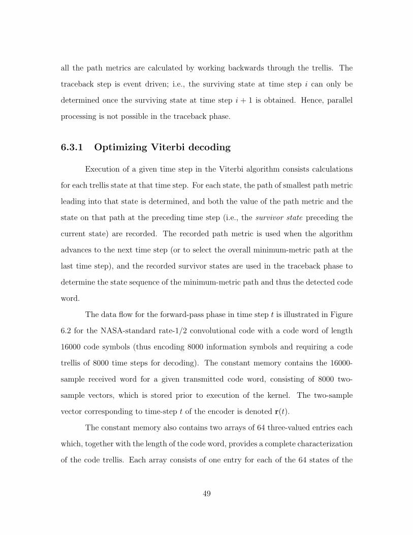
all the path metrics are calculated by working backwards through the trellis. The
traceback step is event driven; i.e., the surviving state at time step i can only be
determined once the surviving state at time step i + 1 is obtained. Hence, parallel
processing is not possible in the traceback phase.
6.3.1 Optimizing Viterbi decoding
Execution of a given time step in the Viterbi algorithm consists calculations
for each trellis state at that time step. For each state, the path of smallest path metric
leading into that state is determined, and both the value of the path metric and the
state on that path at the preceding time step (i.e., the survivor state preceding the
current state) are recorded. The recorded path metric is used when the algorithm
advances to the next time step (or to select the overall minimum-metric path at the
last time step), and the recorded survivor states are used in the traceback phase to
determine the state sequence of the minimum-metric path and thus the detected code
word.
The data flow for the forward-pass phase in time step t is illustrated in Figure
6.2 for the NASA-standard rate-1/2 convolutional code with a code word of length
16000 code symbols (thus encoding 8000 information symbols and requiring a code
trellis of 8000 time steps for decoding). The constant memory contains the 16000-
sample received word for a given transmitted code word, consisting of 8000 two-
sample vectors, which is stored prior to execution of the kernel. The two-sample
vector corresponding to time-step t of the encoder is denoted r(t).
The constant memory also contains two arrays of 64 three-valued entries each
which, together with the length of the code word, provides a complete characterization
of the code trellis. Each array consists of one entry for each of the 64 states of the
49
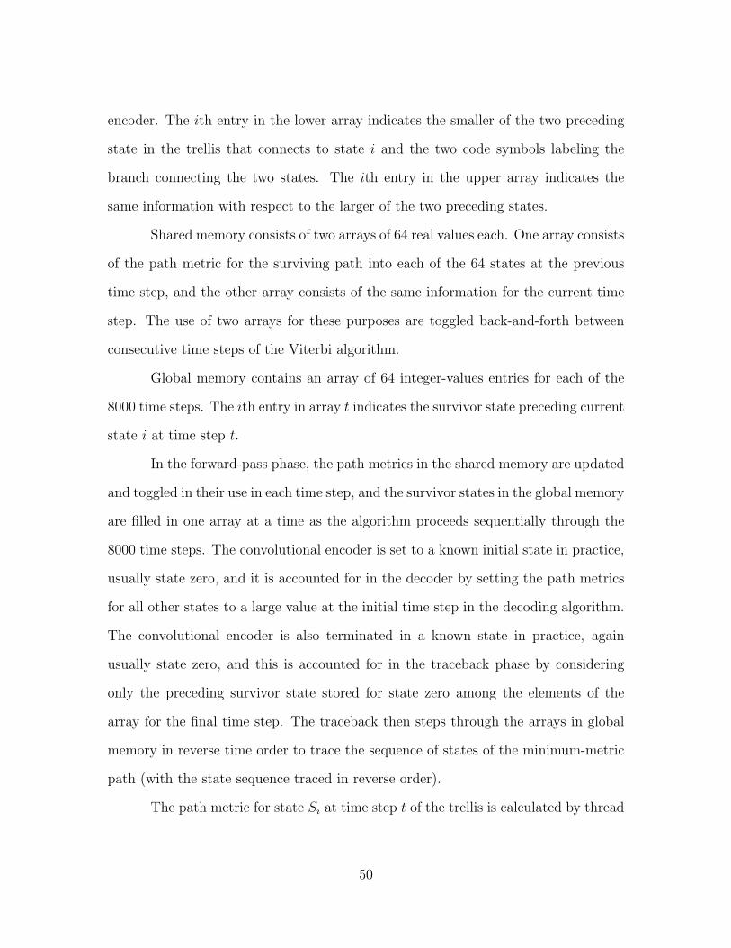
encoder. The ith entry in the lower array indicates the smaller of the two preceding
state in the trellis that connects to state i and the two code symbols labeling the
branch connecting the two states. The ith entry in the upper array indicates the
same information with respect to the larger of the two preceding states.
Shared memory consists of two arrays of 64 real values each. One array consists
of the path metric for the surviving path into each of the 64 states at the previous
time step, and the other array consists of the same information for the current time
step. The use of two arrays for these purposes are toggled back-and-forth between
consecutive time steps of the Viterbi algorithm.
Global memory contains an array of 64 integer-values entries for each of the
8000 time steps. The ith entry in array t indicates the survivor state preceding current
state i at time step t.
In the forward-pass phase, the path metrics in the shared memory are updated
and toggled in their use in each time step, and the survivor states in the global memory
are filled in one array at a time as the algorithm proceeds sequentially through the
8000 time steps. The convolutional encoder is set to a known initial state in practice,
usually state zero, and it is accounted for in the decoder by setting the path metrics
for all other states to a large value at the initial time step in the decoding algorithm.
The convolutional encoder is also terminated in a known state in practice, again
usually state zero, and this is accounted for in the traceback phase by considering
only the preceding survivor state stored for state zero among the elements of the
array for the final time step. The traceback then steps through the arrays in global
memory in reverse time order to trace the sequence of states of the minimum-metric
path (with the state sequence traced in reverse order).
The path metric for state Si at time step t of the trellis is calculated by thread
50
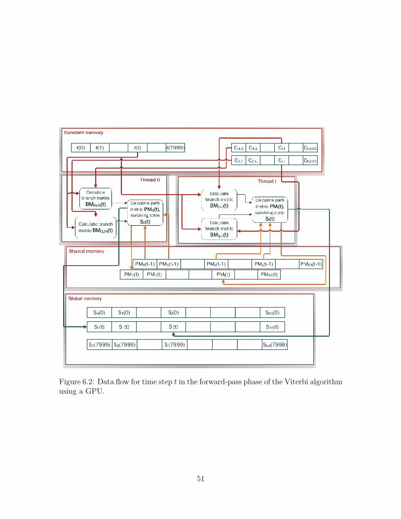
Figure 6.2: Data flow for time step t in the forward-pass phase of the Viterbi algorithmusing a GPU.
51

i at time step t of the algorithm. It is given by
PMSi(t) = min
j(PMSj
(t− 1) + BM(Sj ,Si)(t− 1)×XSj ,Si), 1 ≤ j ≤ N,
where BM(Sj ,Si) is the branch metric between states Sj and Si and Xj,i is a variable
that equals to 1 if there is a connection from state j to i in the trellis diagram and
0 otherwise. The preceding state for state Si in this case will be the state Sj that
results in the minimum (PMSj(t− 1) +BM(Sj ,Si)(t− 1)×XSj ,Si
). The branch metric
is calculated as
BM(Sj ,Si)(t) =
p∑k=0
(r(k)(t)−
√Ec(−1)
c(k)Sj,Si
)2
,
where r(t) is the received vector at time step t and cSj ,Siis the code label for the
branch connecting state Sj to Si.
If all the path metrics of time step (t−1) have been calculated, the path metrics
for all the states in time step t can be calculated at once. Thus, if there are N states
at each time step in the code trellis, a total of N threads can be executed in parallel,
each to calculate the survivor path metric and the preceding survivor state for one
current state. As illustrated for time step t in Figure 6.2, thread 0 uses only the
branch metrics BM(0,0) and BM(1,0) to calculate the path metric and surviving state
for state 0 and thread i calculates the same for state i at the same time. However,
since the path metrics of the previous time step are required to calculate the path
metrics in the current time step, they are calculated one time-step at a time. This
determines the limit of parallelism that is available for the forward-pass phase of the
Viterbi algorithm.
For memory optimization, the received vector, code labels and state connec-
52
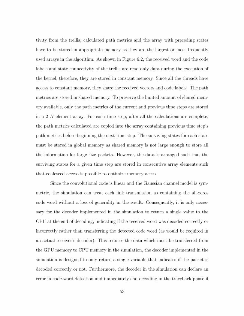
tivity from the trellis, calculated path metrics and the array with preceding states
have to be stored in appropriate memory as they are the largest or most frequently
used arrays in the algorithm. As shown in Figure 6.2, the received word and the code
labels and state connectivity of the trellis are read-only data during the execution of
the kernel; therefore, they are stored in constant memory. Since all the threads have
access to constant memory, they share the received vectors and code labels. The path
metrics are stored in shared memory. To preserve the limited amount of shared mem-
ory available, only the path metrics of the current and previous time steps are stored
in a 2 N -element array. For each time step, after all the calculations are complete,
the path metrics calculated are copied into the array containing previous time step’s
path metrics before beginning the next time step. The surviving states for each state
must be stored in global memory as shared memory is not large enough to store all
the information for large size packets. However, the data is arranged such that the
surviving states for a given time step are stored in consecutive array elements such
that coalesced access is possible to optimize memory access.
Since the convolutional code is linear and the Gaussian channel model is sym-
metric, the simulation can treat each link transmission as containing the all-zeros
code word without a loss of generality in the result. Consequently, it is only neces-
sary for the decoder implemented in the simulation to return a single value to the
CPU at the end of decoding, indicating if the received word was decoded correctly or
incorrectly rather than transferring the detected code word (as would be required in
an actual receiver’s decoder). This reduces the data which must be transferred from
the GPU memory to CPU memory in the simulation, the decoder implemented in the
simulation is designed to only return a single variable that indicates if the packet is
decoded correctly or not. Furthermore, the decoder in the simulation can declare an
error in code-word detection and immediately end decoding in the traceback phase if
53
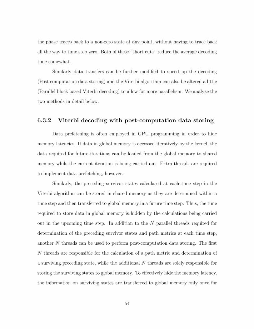
the phase traces back to a non-zero state at any point, without having to trace back
all the way to time step zero. Both of these “short cuts” reduce the average decoding
time somewhat.
Similarly data transfers can be further modified to speed up the decoding
(Post computation data storing) and the Viterbi algorithm can also be altered a little
(Parallel block based Viterbi decoding) to allow for more parallelism. We analyze the
two methods in detail below.
6.3.2 Viterbi decoding with post-computation data storing
Data prefetching is often employed in GPU programming in order to hide
memory latencies. If data in global memory is accessed iteratively by the kernel, the
data required for future iterations can be loaded from the global memory to shared
memory while the current iteration is being carried out. Extra threads are required
to implement data prefetching, however.
Similarly, the preceding survivor states calculated at each time step in the
Viterbi algorithm can be stored in shared memory as they are determined within a
time step and then transferred to global memory in a future time step. Thus, the time
required to store data in global memory is hidden by the calculations being carried
out in the upcoming time step. In addition to the N parallel threads required for
determination of the preceding survivor states and path metrics at each time step,
another N threads can be used to perform post-computation data storing. The first
N threads are responsible for the calculation of a path metric and determination of
a surviving preceding state, while the additional N threads are solely responsible for
storing the surviving states to global memory. To effectively hide the memory latency,
the information on surviving states are transferred to global memory only once for
54
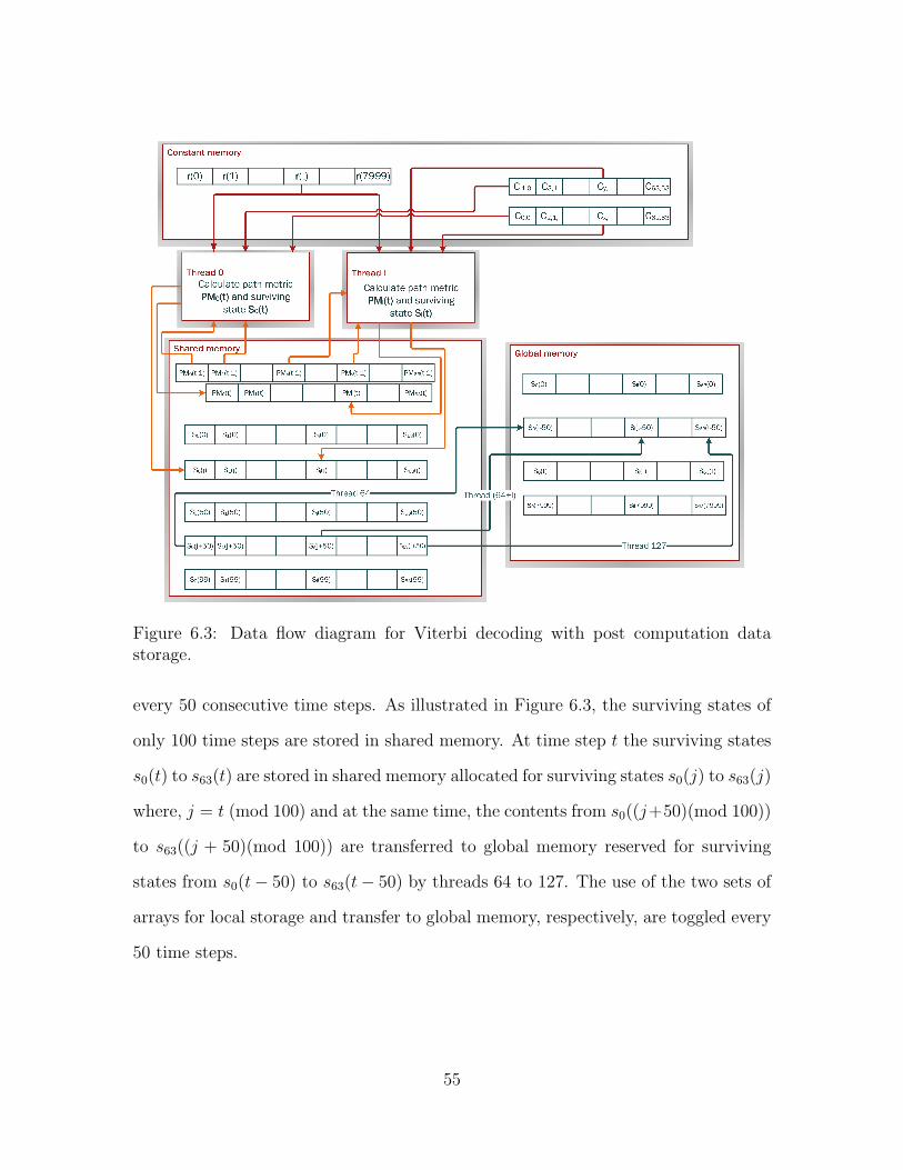
Figure 6.3: Data flow diagram for Viterbi decoding with post computation datastorage.
every 50 consecutive time steps. As illustrated in Figure 6.3, the surviving states of
only 100 time steps are stored in shared memory. At time step t the surviving states
s0(t) to s63(t) are stored in shared memory allocated for surviving states s0(j) to s63(j)
where, j = t (mod 100) and at the same time, the contents from s0((j+50)(mod 100))
to s63((j + 50)(mod 100)) are transferred to global memory reserved for surviving
states from s0(t− 50) to s63(t− 50) by threads 64 to 127. The use of the two sets of
arrays for local storage and transfer to global memory, respectively, are toggled every
50 time steps.
55
6.3.3 Parallel block based Viterbi decoding
The growing interest in parallel architectures (including GPUs) for decoder
implementation has included recent investigation of Viterbi decoding implementation
on a GPU using CUDA [15][16] as well as ways to adapt the algorithm to the GPU.
The parallel block based Viterbi decoding (PBVD) [17] divides the received word into
small blocks called parallel blocks and decodes the individual blocks independently.
Each parallel block has three parts: an initial part is called the truncated block,
a middle part called the decoded block, and a final part called the traceback block.
The truncated and traceback blocks represent segments that overlap with blocks
immediately before and after the current block in the receiver word, respectively.
The overlapping of the blocks allows the application of the forward-pass and traceback
phases of the Viterbi algorithm of each parallel block to start from a random state in
the code trellis without significantly impacting probability of correctly decoding the
decoded block. The length of the truncated and traceback blocks are typically five
times the constraint length of the code.
The PBVD algorithm is well suited to the effective utilization of the resources
of a GPU. If a received word is divided into M blocks, N×M threads can be launched
with N threads responsible for a single block. This method allows the user to use
more of the GPU resources available for decoding a single received word.
6.4 Performance evaluation of various optimiza-
tion techniques
In this section, we consider the optimization techniques discussed in the previ-
ous section using the simulation of a simple network consisting of a single transmitter
56
and a receiver. It is seen in Figure 6.4 that each of the methods of simulating the
decoder performance results in essentially the same probability of code-word error.
Consequently, we can focus on the simulation time as the sole basis of comparison
of the methods. The average time required to decode 1000 received words is used
to compare the speed of the various decoding techniques and is also used to obtain
the best decoder suitable for integration with ns-3. Simulation for each decoding
technique is carried out until 1000 packets are received in error.
Figure 6.5 and 6.6 show the average simulation time to decode 1000 received
words for different decoding techniques and code-word sizes. A 16-core 2.70 GHz
Intel Xeon E5-2680 CPU with two 810 MHz NVIDIA TESLA k40 GPUs is used for
all the simulations in this section. The top figure in Figure 6.5, shows the simulation
time for code words of size16000 bits. The average simulation time for decoding with
a CPU is 11.2 s for any value of the signal-to-noise ratio. When GPU processing is
used, the simulation time is reduced. First consider a naive utilization of the GPU
in which global memory is used for all of the larger arrays and no attempt is made
to arrange the data in a manner to facilitate coalesced memory access. This is the
circumstance denoted by “decoding without memory optimizations” in the figures. It
results in a simulation time of 6.7 s, which a reduction of less than one-half in time
required with the CPU.
The use of the GPU with reasonable memory management results in a some-
what lower simulation time. Using constant memory, shared memory and arranging
the data before storing them in global memory to facilitate coalesced memory access
reduces the simulation time to 4.9 s. Furthermore, if post-computation data storage
is used to hide memory latency, the simulation time decreases to 3 seconds. And
finally, if the PBVD algorithm is used, the simulation time is reduced substantially to
0.89 s. In this implementation of the PBVD algorithm, the received word is divided
57

into blocks of 250 bits plus 35 bits of truncated and traceback blocks added in front
and back of each block where necessary. In all the decoding techniques other than the
PBVD algorithm, the path metrics for each time step are calculated serially. Thus
altogether 16000 “for” loops are carried out in the forward-pass phase serially by each
thread. But in the PBVD algorithm a single thread carries out a maximum of 160
loops serially in the forward-pass phase. This allows for the simulation time to reduce
drastically especially in large packets.
From Figure 6.5 it can be observed that the two most suitable techniques that
can be integrated into ns-3 are the decoding with post-computation data storage and
the PBVD algorithm. The PBVD algorithm is very efficient for decoding large code
words, as seen above. We also compare the simulation time for the two techniques
for code-word sizes of 200, 2000 and 8000 bits. The bottom figure in Figure 6.5
shows the simulation time for a code word of size 200 bits. Since the code word
size is smaller than 250 bits, the PBVD algorithm is carried out in a single block and
essentially it reduces to Viterbi decoding with memory optimization but without data
post computation storing. It can be seen that the time required to execute the PBVD
algorithm on a GPU is almost the same as the time required by the Viterbi algorithm
on a CPU. For some values of SNR, the time required using GPU is even slightly
larger than the time required by a CPU. Similarly, using the GPU with memory
optimization and post computation data storing only reduces simulation time by
0.02 seconds. This shows that when the code-word length is very small, there is no
speed up in the simulation using a GPU. The time saved by carrying out parallel
computations are balanced by the time required for all the data transfers.
Figure 6.6 shows the simulation time for code-word sizes 2000 and 8000 bits.
It can be observed that as code-word sizes increase, the advantages of using a GPU
becomes more evident. The PBVD algorithm also results in faster simulation time
58

as the code-word size increases. For a code-word size of 2000 bits, employing a
GPU reduces the simulation time to one-third of the time required with a CPU,
whereas for a code-word size of 8000 bits, the simulation is reduced to one-eight that
with the CPU. It is clear that the PBVD algorithm has the potential to provide the
highest speed-up over a broad range of circumstances when integrated into a network
simulation. Hence, for rest of the dissertation we focus on the use of PBVD algorithm
for decoding in the networks using convolutional coding.
Theoretically, the speed up in simulation using parallel processing should be
in the order of the number of threads launched for parallel processing as shown by the
computational complexity in Appendix A. However, there are many factors that limit
the increase in speed of a simulation. Data transfer between CPU and GPU memory
before and after each kernel launch, time required to launch a CUDA kernel and
setup arguments create an overhead when using a GPU. The type of memory being
accessed by the kernel also governs the speed of the simulation. Memory optimization
can reduce unnecessary off-chip memory access that has the potential to slow down a
program, but unavoidable off-chip memory access will still hinder speed-ups. Another
important factor is the occupancy percentage of a kernel. Occupancy is a measure
of the number of concurrent warps launched in an SM. A GPU hides memory access
latency with computations of other warps launched concurrently. If the occupancy is
low, the warps of threads launched are not sufficient to hide all the memory latency,
thus limiting the speed up of the code. In our simulation for the Viterbi decoding with
post computation data storage, the occupancy is 8% and for the PBVD simulation
it is 33%. The large shared memory required by for post computation data storage
and the limited number of threads that can be launched for Viterbi decoding limits
the occupancy of our simulation, thus affecting the overall speedup.
59
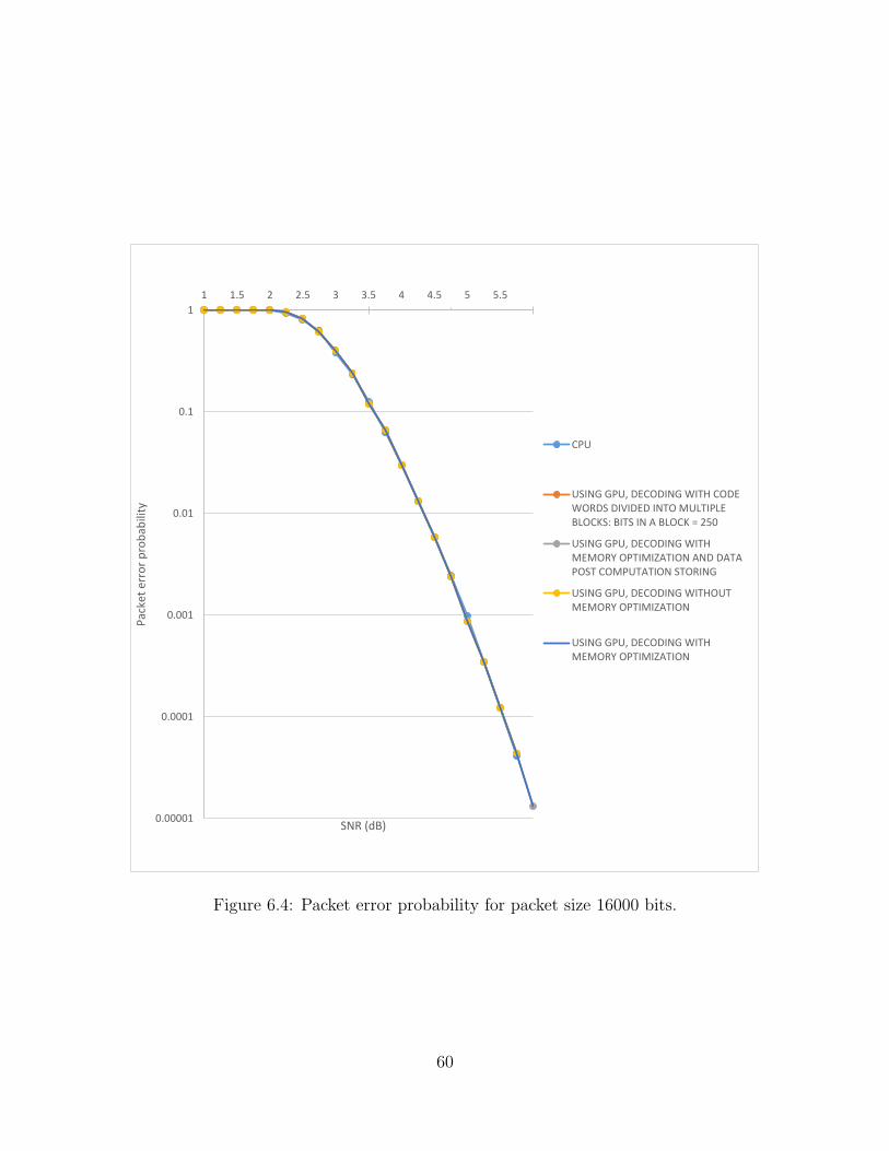
0.00001
0.0001
0.001
0.01
0.1
1
1 1.5 2 2.5 3 3.5 4 4.5 5 5.5
Pa
cke
t e
rro
r p
rob
ab
ilit
y
SNR (dB)
CPU
USING GPU, DECODING WITH CODE
WORDS DIVIDED INTO MULTIPLE
BLOCKS: BITS IN A BLOCK = 250
USING GPU, DECODING WITH
MEMORY OPTIMIZATION AND DATA
POST COMPUTATION STORING
USING GPU, DECODING WITHOUT
MEMORY OPTIMIZATION
USING GPU, DECODING WITH
MEMORY OPTIMIZATION
Figure 6.4: Packet error probability for packet size 16000 bits.
60
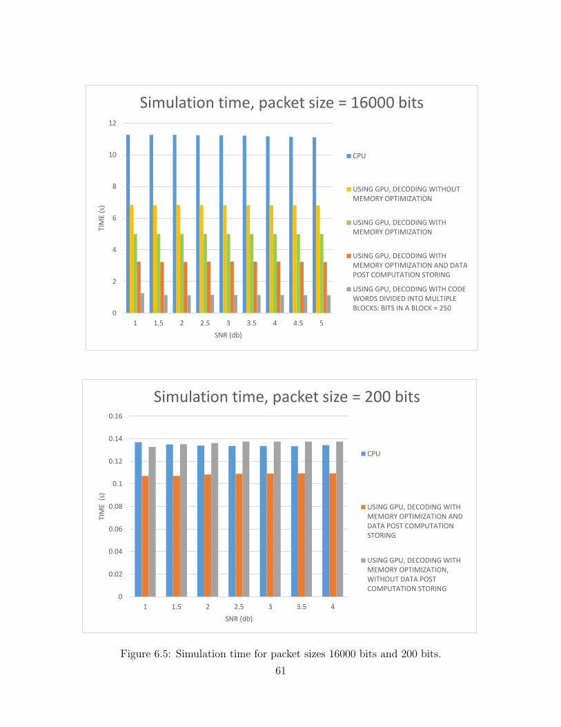
0
2
4
6
8
10
12
1 1.5 2 2.5 3 3.5 4 4.5 5
TIM
E (
s)
SNR (db)
Simulation time, packet size = 16000 bits
CPU
USING GPU, DECODING WITHOUT
MEMORY OPTIMIZATION
USING GPU, DECODING WITH
MEMORY OPTIMIZATION
USING GPU, DECODING WITH
MEMORY OPTIMIZATION AND DATA
POST COMPUTATION STORING
USING GPU, DECODING WITH CODE
WORDS DIVIDED INTO MULTIPLE
BLOCKS: BITS IN A BLOCK = 250
0
0.02
0.04
0.06
0.08
0.1
0.12
0.14
0.16
1 1.5 2 2.5 3 3.5 4
TIM
E (s
)
SNR (db)
Simulation time, packet size = 200 bits
CPU
USING GPU, DECODING WITH
MEMORY OPTIMIZATION AND
DATA POST COMPUTATION
STORING
USING GPU, DECODING WITH
MEMORY OPTIMIZATION,
WITHOUT DATA POST
COMPUTATION STORING
Figure 6.5: Simulation time for packet sizes 16000 bits and 200 bits.
61
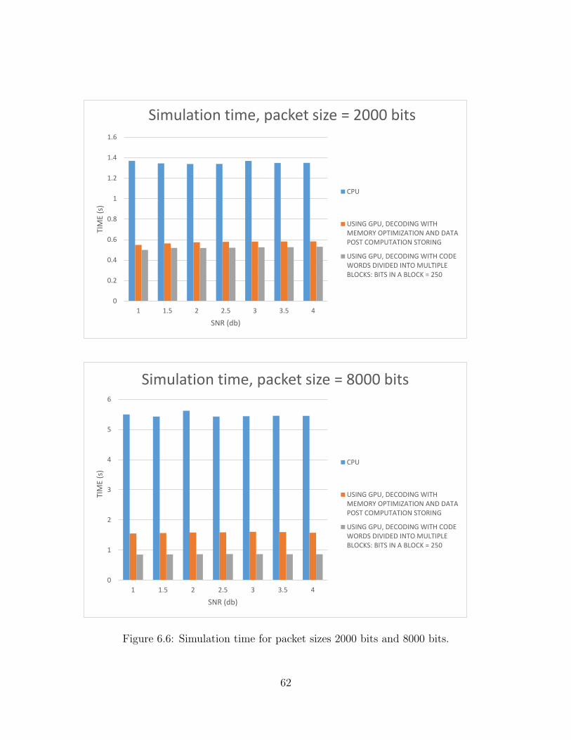
0
0.2
0.4
0.6
0.8
1
1.2
1.4
1.6
1 1.5 2 2.5 3 3.5 4
TIM
E (
s)
SNR (db)
Simulation time, packet size = 2000 bits
CPU
USING GPU, DECODING WITH
MEMORY OPTIMIZATION AND DATA
POST COMPUTATION STORING
USING GPU, DECODING WITH CODE
WORDS DIVIDED INTO MULTIPLE
BLOCKS: BITS IN A BLOCK = 250
0
1
2
3
4
5
6
1 1.5 2 2.5 3 3.5 4
TIM
E (
s)
SNR (db)
Simulation time, packet size = 8000 bits
CPU
USING GPU, DECODING WITH
MEMORY OPTIMIZATION AND DATA
POST COMPUTATION STORING
USING GPU, DECODING WITH CODE
WORDS DIVIDED INTO MULTIPLE
BLOCKS: BITS IN A BLOCK = 250
Figure 6.6: Simulation time for packet sizes 2000 bits and 8000 bits.
62
Chapter 7
Network Simulation with
GPU-Accelerated Viterbi Decoding
As seen in the previous chapter, the use of a GPU can substantially reduce the
time required for bit-accurate on-line simulation of Viterbi decoding in comparison
with the use of a CPU alone. The reduction in simulation is especially marked if
appropriate memory management techniques are employed with GPU programming
and if the PBVD modification of the Viterbi decoder is used to exploit the available
parallelism of the GPU more effectively. In this chapter, we consider the incorporation
of a GPU into the simulation of the small network, where it is used to implement bit-
accurate on-line simulation of the PBVD algorithm. The accuracy of the simulation is
investigated, and the simulation time that results is compared with the other methods
we have considered in the previous chapters. We also consider a modification of the
simulation that eliminates the need to simulate some packet reception outcomes, and
we consider a modification that permits a further improvement in the utilization of
the GPUs resources with the PBVD algorithm.
The code for the PBVD algorithm is written in CUDA C source files. They
63
can be integrated with ns-3 by modifying the wscript script file of ns-3. (In this
manner, CUDA functions can be added or used to replace any existing functions in
ns-3.) The PBVD function written in CUDA thus serves as a “drop in” replacement
for the C++ code Viterbi decoder (written for execution on a CPU) in the network
simulation.
7.1 Accelerating network simulation with PBVD
algorithm
7.1.1 Concurrent PBVD algorithm
In a deployment of the 802.11b MAC protocol, a transmitted packet may be
acquired by each listening network node that is near the transmitter, resulting in each
of them decoding the received word for the packet. A characteristic of each of the link
simulation approaches considered thus far is the fact that the outcomes for a given
packet transmission are determined sequentially for different nodes that attempt to
decode the packet’s payload. If a GPU is used to implement bit-accurate on-line
simulation of the Viterbi decoder or PBVD algorithm, however, only a fraction of the
GPU computational resources are used. If the network simulation can be modified
to permit parallel execution of multiple instances of the decoding algorithm without
compromising the fidelity of the simulation, a reduction in the simulation time may
be possible.
Implementation of parallel decoding of the received words at all nodes for a
given packet transmission requires a reordering of actions in the ns-3 simulation. In
particular, the difference in propagation delays across the different links for the trans-
mission results in a delay of decoding until all the nodes have received the complete
64
transmission. At that time, a single global function is called to execute parallel de-
coding on the GPU. A decoded word is returned for each of the nodes on completion
and the simulation proceeds. We refer to this as concurrent PBVD.
7.1.2 Selective decoding
For a given data packet transmission, not all of the nearby nodes which decode
the received word are intended recipients of the packet. If decoding fails at such a node
(or any node), the packet is dropped immediately. If instead, the payload is decoded
in the physical layer, it is passed to its MAC sub-layer for subsequent processing.
The destination MAC address of the received packet is examined in the MAC layer,
and if the packet’s destination address does not match the node’s MAC address, it is
dropped after updating the node’s Network Allocation Vector (NAV).
In a full implementation of the protocol in a simulation, it is apparent that
significant simulation time may be expended determining decoder outcomes for data
packets at third-party receiving nodes that of necessity result in either decoder fail-
ure or a packet drop after an NAV update. An alternative, which we denote selective
decoding, simplifies the network simulation’s model of outcomes for the reception of
a data packet at a node other than the packet’s intended destination(s). In selective
decoding, the physical-layer payload of such a data packet is assumed to be detected
correctly at each third-party node without simulating the decoder so that it is always
passed to the MAC layer of the node. The selective decoding approach is only applied
to data packets. (Applying it to RTS/CTS, ACK and other packets that are broad-
cast, such as OLSR packets, could alter MAC behavior in the network in a way that
would compromise the fidelity of the simulation.) Thus, a data packet is assumed
to be decoded correctly without simulating the coder if the received packet is a data
65
packet, the destination address does not match the node’s address, and the received
transmission is not a broadcast.
7.2 Network simulation performance with the PBVD
algorithm
The network performance with bit-accurate on-line simulation of the Viterbi
algorithm using a CPU serves as the benchmark for assessment of the performance
with on-line simulation of the PBVD algorithm using a GPU. The throughput of flow
1 in the small network is shown for both simulation approaches in Figure 7.1. It is
seen that the two methods result in a negligible difference in the simulated throughput
under each condition considered, which is consistent with the comparison of the two
in the previous chapter for a single link isolation (as seen in Figure 6.4).
Table 7.1 shows the time required to simulate one second of network activity
in the small network for the different link models. Two positions and two interference
probabilities for the interfering jammer are considered. The PBVD algorithm imple-
mented on the GPU results in a reduction in the simulation time by more than a factor
of 10 compared with Viterbi decoding implemented on the CPU without any effect on
the simulated throughput. It requires approximately twice the simulation time of the
tighter concave-Chernoff bound but somewhat less than the concave-integral bound,
even though the latter two methods results in less accurate throughput. As with the
other methods, the PBVD algorithm on the GPU results in a higher simulation time
than if the SINR threshold is used, but the latter yields simulation results of greatly
reduced accuracy for some network conditions.
The effect of implementing concurrent PBVD in the GPU on the performance
66
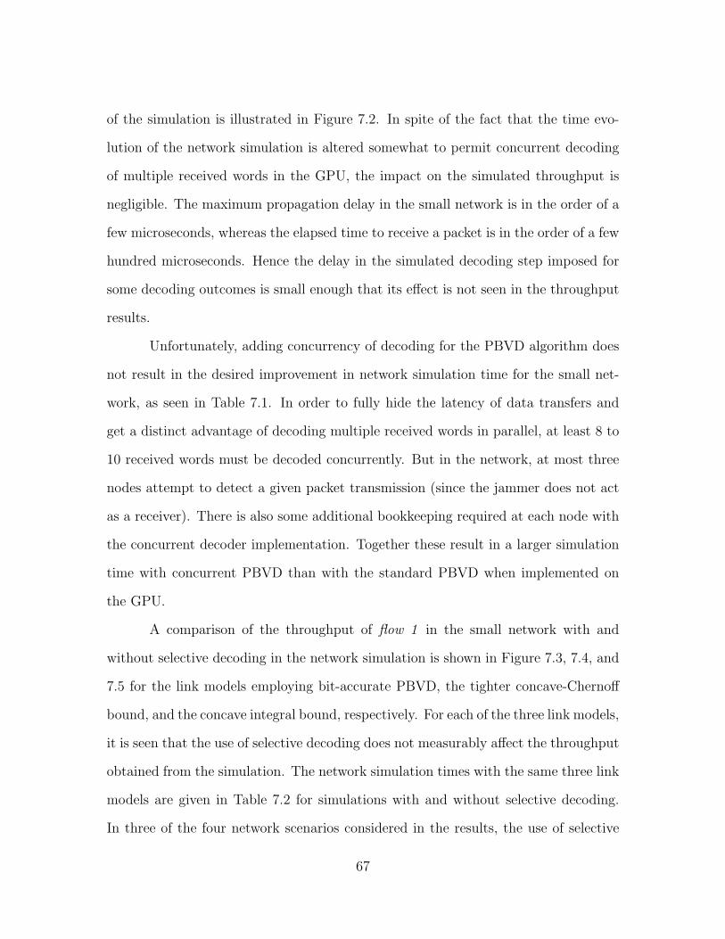
of the simulation is illustrated in Figure 7.2. In spite of the fact that the time evo-
lution of the network simulation is altered somewhat to permit concurrent decoding
of multiple received words in the GPU, the impact on the simulated throughput is
negligible. The maximum propagation delay in the small network is in the order of a
few microseconds, whereas the elapsed time to receive a packet is in the order of a few
hundred microseconds. Hence the delay in the simulated decoding step imposed for
some decoding outcomes is small enough that its effect is not seen in the throughput
results.
Unfortunately, adding concurrency of decoding for the PBVD algorithm does
not result in the desired improvement in network simulation time for the small net-
work, as seen in Table 7.1. In order to fully hide the latency of data transfers and
get a distinct advantage of decoding multiple received words in parallel, at least 8 to
10 received words must be decoded concurrently. But in the network, at most three
nodes attempt to detect a given packet transmission (since the jammer does not act
as a receiver). There is also some additional bookkeeping required at each node with
the concurrent decoder implementation. Together these result in a larger simulation
time with concurrent PBVD than with the standard PBVD when implemented on
the GPU.
A comparison of the throughput of flow 1 in the small network with and
without selective decoding in the network simulation is shown in Figure 7.3, 7.4, and
7.5 for the link models employing bit-accurate PBVD, the tighter concave-Chernoff
bound, and the concave integral bound, respectively. For each of the three link models,
it is seen that the use of selective decoding does not measurably affect the throughput
obtained from the simulation. The network simulation times with the same three link
models are given in Table 7.2 for simulations with and without selective decoding.
In three of the four network scenarios considered in the results, the use of selective
67
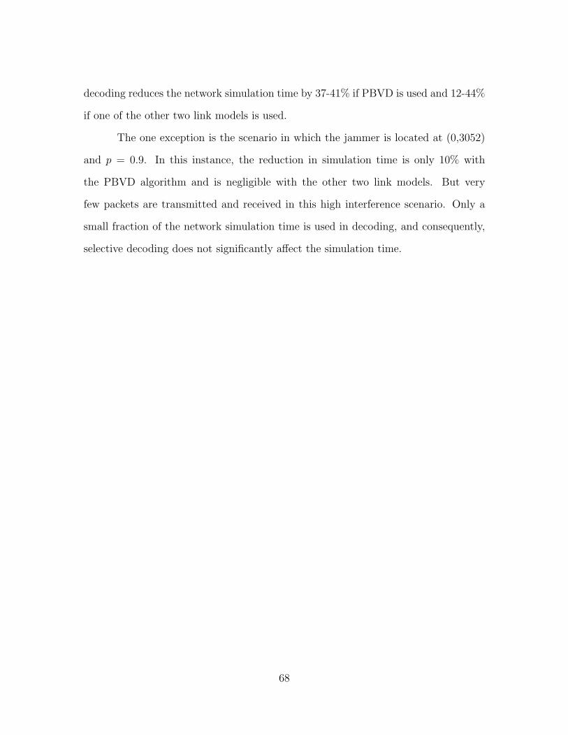
decoding reduces the network simulation time by 37-41% if PBVD is used and 12-44%
if one of the other two link models is used.
The one exception is the scenario in which the jammer is located at (0,3052)
and p = 0.9. In this instance, the reduction in simulation time is only 10% with
the PBVD algorithm and is negligible with the other two link models. But very
few packets are transmitted and received in this high interference scenario. Only a
small fraction of the network simulation time is used in decoding, and consequently,
selective decoding does not significantly affect the simulation time.
68
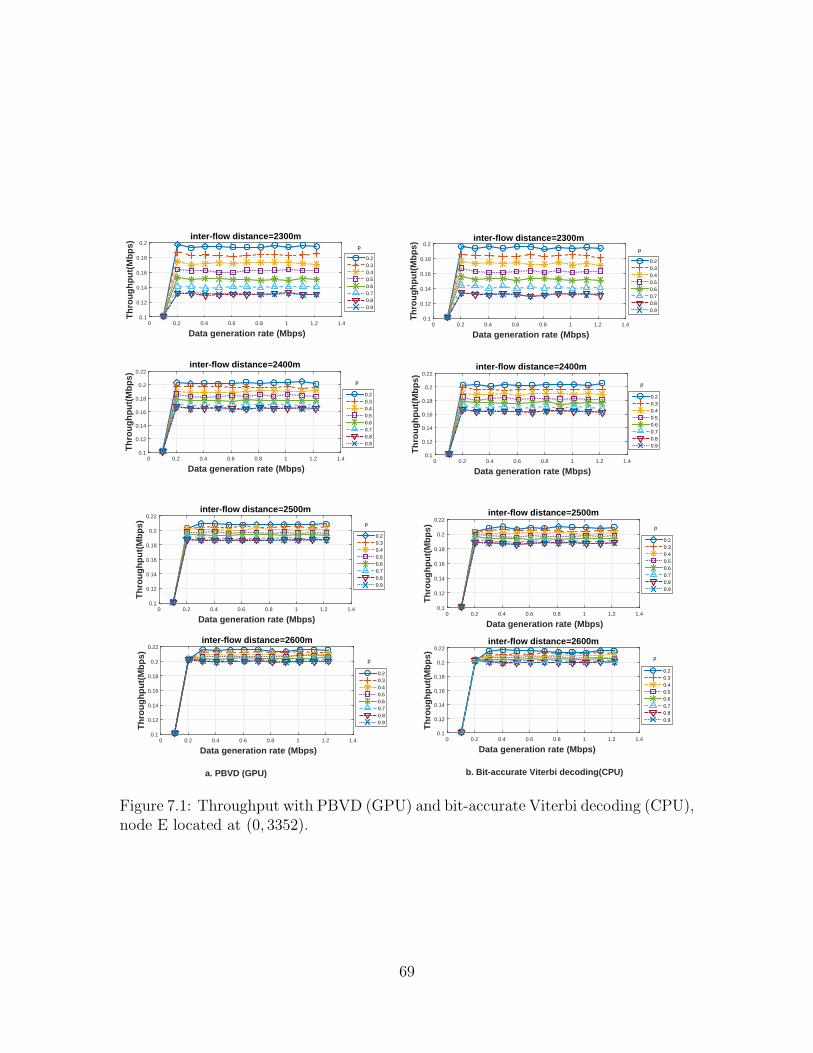
Data generation rate (Mbps)0 0.2 0.4 0.6 0.8 1 1.2 1.4
Th
rou
gh
pu
t(M
bp
s)
0.1
0.12
0.14
0.16
0.18
0.2inter-flow distance=2300m
0.20.30.40.50.60.70.80.9
Data generation rate (Mbps)0 0.2 0.4 0.6 0.8 1 1.2 1.4
Th
rou
gh
pu
t(M
bp
s)
0.1
0.12
0.14
0.16
0.18
0.2inter-flow distance=2300m
0.20.30.40.50.60.70.80.9
Data generation rate (Mbps)0 0.2 0.4 0.6 0.8 1 1.2 1.4
Th
rou
gh
pu
t(M
bp
s)
0.1
0.12
0.14
0.16
0.18
0.2
0.22inter-flow distance=2400m
0.20.30.40.50.60.70.80.9
Data generation rate (Mbps)0 0.2 0.4 0.6 0.8 1 1.2 1.4
Th
rou
gh
pu
t(M
bp
s)
0.1
0.12
0.14
0.16
0.18
0.2
0.22inter-flow distance=2400m
0.20.30.40.50.60.70.80.9
p p
p p
Data generation rate (Mbps)0 0.2 0.4 0.6 0.8 1 1.2 1.4
Th
rou
gh
pu
t(M
bp
s)
0.1
0.12
0.14
0.16
0.18
0.2
0.22inter-flow distance=2500m
0.20.30.40.50.60.70.80.9
Data generation rate (Mbps)0 0.2 0.4 0.6 0.8 1 1.2 1.4
Th
rou
gh
pu
t(M
bp
s)
0.1
0.12
0.14
0.16
0.18
0.2
0.22inter-flow distance=2500m
0.20.30.40.50.60.70.80.9
Data generation rate (Mbps)
a. PBVD (GPU)
0 0.2 0.4 0.6 0.8 1 1.2 1.4
Th
rou
gh
pu
t(M
bp
s)
0.1
0.12
0.14
0.16
0.18
0.2
0.22inter-flow distance=2600m
0.20.30.40.50.60.70.80.9
Data generation rate (Mbps)
b. Bit-accurate Viterbi decoding(CPU)
0 0.2 0.4 0.6 0.8 1 1.2 1.4
Th
rou
gh
pu
t(M
bp
s)
0.1
0.12
0.14
0.16
0.18
0.2
0.22inter-flow distance=2600m
0.20.30.40.50.60.70.80.9
pp
pp
Figure 7.1: Throughput with PBVD (GPU) and bit-accurate Viterbi decoding (CPU),node E located at (0, 3352).
69
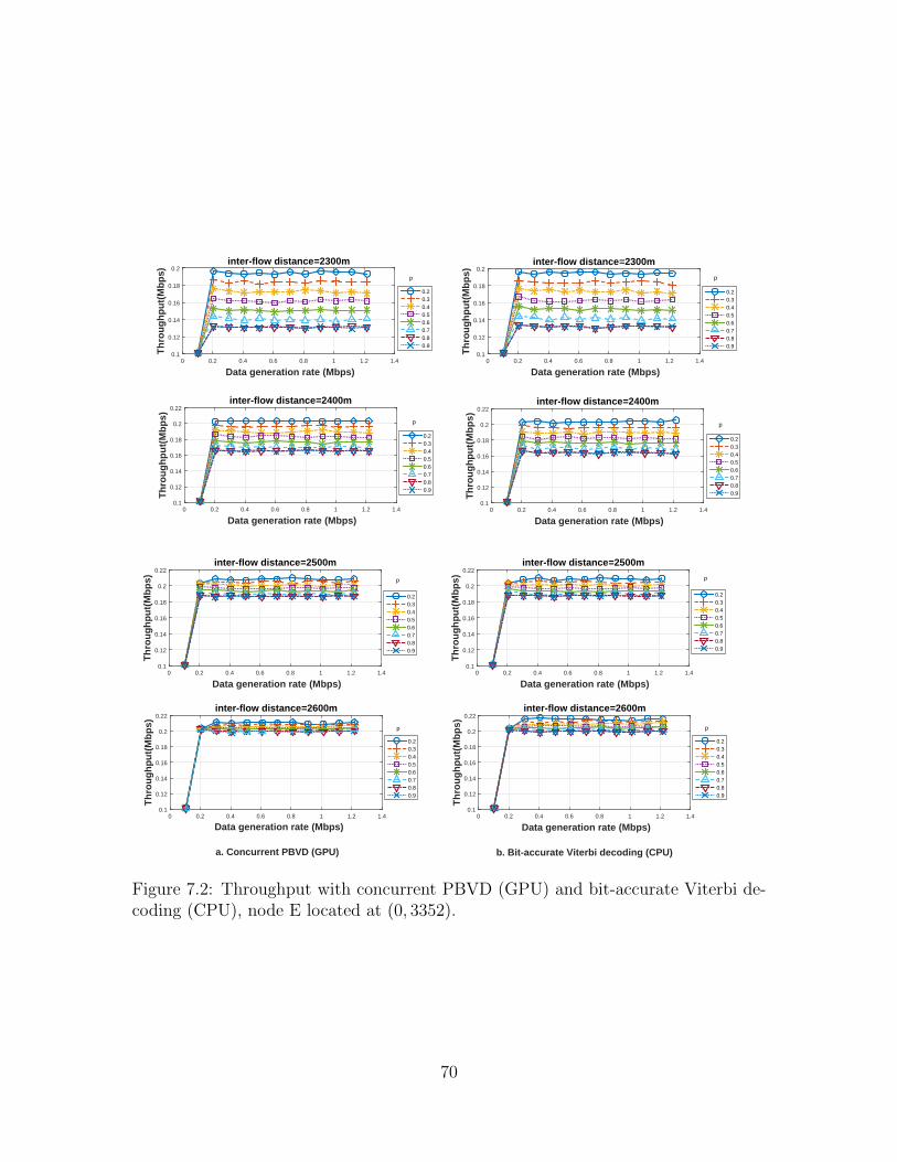
Data generation rate (Mbps)0 0.2 0.4 0.6 0.8 1 1.2 1.4
Th
rou
gh
pu
t(M
bp
s)
0.1
0.12
0.14
0.16
0.18
0.2inter-flow distance=2300m
0.20.30.40.50.60.70.80.9
Data generation rate (Mbps)0 0.2 0.4 0.6 0.8 1 1.2 1.4
Th
rou
gh
pu
t(M
bp
s)
0.1
0.12
0.14
0.16
0.18
0.2
0.22inter-flow distance=2400m
0.20.30.40.50.60.70.80.9
Data generation rate (Mbps)0 0.2 0.4 0.6 0.8 1 1.2 1.4
Th
rou
gh
pu
t(M
bp
s)
0.1
0.12
0.14
0.16
0.18
0.2
0.22inter-flow distance=2400m
0.20.30.40.50.60.70.80.9
Data generation rate (Mbps)0 0.2 0.4 0.6 0.8 1 1.2 1.4
Th
rou
gh
pu
t(M
bp
s)
0.1
0.12
0.14
0.16
0.18
0.2inter-flow distance=2300m
0.20.30.40.50.60.70.80.9
p p
p p
Data generation rate (Mbps)0 0.2 0.4 0.6 0.8 1 1.2 1.4
Th
rou
gh
pu
t(M
bp
s)
0.1
0.12
0.14
0.16
0.18
0.2
0.22inter-flow distance=2500m
0.20.30.40.50.60.70.80.9
Data generation rate (Mbps)0 0.2 0.4 0.6 0.8 1 1.2 1.4
Th
rou
gh
pu
t(M
bp
s)
0.1
0.12
0.14
0.16
0.18
0.2
0.22inter-flow distance=2500m
0.20.30.40.50.60.70.80.9
Data generation rate (Mbps)
a. Concurrent PBVD (GPU)
0 0.2 0.4 0.6 0.8 1 1.2 1.4
Th
rou
gh
pu
t(M
bp
s)
0.1
0.12
0.14
0.16
0.18
0.2
0.22inter-flow distance=2600m
0.20.30.40.50.60.70.80.9
Data generation rate (Mbps)
b. Bit-accurate Viterbi decoding (CPU)
0 0.2 0.4 0.6 0.8 1 1.2 1.4
Th
rou
gh
pu
t(M
bp
s)
0.1
0.12
0.14
0.16
0.18
0.2
0.22inter-flow distance=2600m
0.20.30.40.50.60.70.80.9
pp
p p
Figure 7.2: Throughput with concurrent PBVD (GPU) and bit-accurate Viterbi de-coding (CPU), node E located at (0, 3352).
70
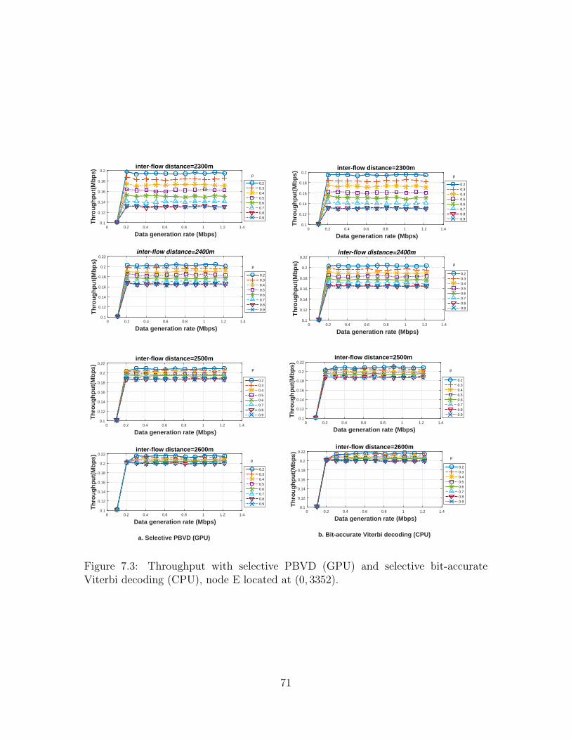
Data generation rate (Mbps)0 0.2 0.4 0.6 0.8 1 1.2 1.4
Th
rou
gh
pu
t(M
bp
s)
0.1
0.12
0.14
0.16
0.18
0.2inter-flow distance=2300m
0.20.30.40.50.60.70.80.9
Data generation rate (Mbps)0 0.2 0.4 0.6 0.8 1 1.2 1.4
Th
rou
gh
pu
t(M
bp
s)
0.1
0.12
0.14
0.16
0.18
0.2
0.22inter-flow distance=2400m
0.20.30.40.50.60.70.80.9
Data generation rate (Mbps)0 0.2 0.4 0.6 0.8 1 1.2 1.4
Th
rou
gh
pu
t(M
bp
s)
0.1
0.12
0.14
0.16
0.18
0.2
0.22inter-flow distance=2400m
0.20.30.40.50.60.70.80.9
Data generation rate (Mbps)0 0.2 0.4 0.6 0.8 1 1.2 1.4
Th
rou
gh
pu
t(M
bp
s)
0.1
0.12
0.14
0.16
0.18
0.2inter-flow distance=2300m
0.20.30.40.50.60.70.80.9
p p
pp
Data generation rate (Mbps)0 0.2 0.4 0.6 0.8 1 1.2 1.4
Th
rou
gh
pu
t(M
bp
s)
0.1
0.12
0.14
0.16
0.18
0.2
0.22inter-flow distance=2500m
0.20.30.40.50.60.70.80.9
Data generation rate (Mbps)0 0.2 0.4 0.6 0.8 1 1.2 1.4
Th
rou
gh
pu
t(M
bp
s)
0.1
0.12
0.14
0.16
0.18
0.2
0.22inter-flow distance=2500m
0.20.30.40.50.60.70.80.9
Data generation rate (Mbps)
a. Selective PBVD (GPU)
0 0.2 0.4 0.6 0.8 1 1.2 1.4
Th
rou
gh
pu
t(M
bp
s)
0.1
0.12
0.14
0.16
0.18
0.2
0.22inter-flow distance=2600m
0.20.30.40.50.60.70.80.9
Data generation rate (Mbps)
b. Bit-accurate Viterbi decoding (CPU)
0 0.2 0.4 0.6 0.8 1 1.2 1.4
Th
rou
gh
pu
t(M
bp
s)
0.1
0.12
0.14
0.16
0.18
0.2
0.22inter-flow distance=2600m
0.20.30.40.50.60.70.80.9
pp
pp
Figure 7.3: Throughput with selective PBVD (GPU) and selective bit-accurateViterbi decoding (CPU), node E located at (0, 3352).
71
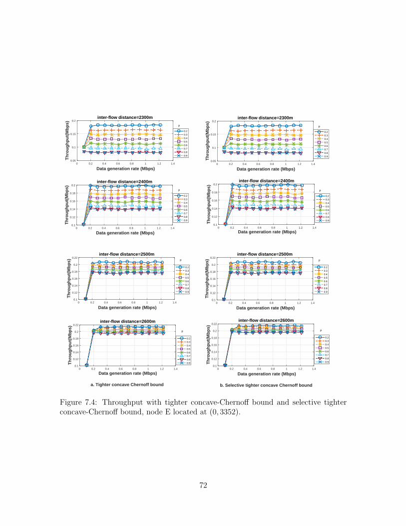
Data generation rate (Mbps)0 0.2 0.4 0.6 0.8 1 1.2 1.4
Th
rou
gh
pu
t(M
bp
s)
0.05
0.1
0.15
0.2inter-flow distance=2300m
0.20.30.40.50.60.70.80.9
Data generation rate (Mbps)0 0.2 0.4 0.6 0.8 1 1.2 1.4
Th
rou
gh
pu
t(M
bp
s)
0.05
0.1
0.15
0.2inter-flow distance=2300m
0.20.30.40.50.60.70.80.9
Data generation rate (Mbps)0 0.2 0.4 0.6 0.8 1 1.2 1.4
Th
rou
gh
pu
t(M
bp
s)
0.1
0.12
0.14
0.16
0.18
0.2inter-flow distance=2400m
0.20.30.40.50.60.70.80.9
Data generation rate (Mbps)0 0.2 0.4 0.6 0.8 1 1.2 1.4
Th
rou
gh
pu
t(M
bp
s)
0.1
0.12
0.14
0.16
0.18
0.2inter-flow distance=2400m
0.20.30.40.50.60.70.80.9
p p
p p
Data generation rate (Mbps)0 0.2 0.4 0.6 0.8 1 1.2 1.4
Th
rou
gh
pu
t(M
bp
s)
0.1
0.12
0.14
0.16
0.18
0.2
0.22inter-flow distance=2500m
0.20.30.40.50.60.70.80.9
Data generation rate (Mbps)0 0.2 0.4 0.6 0.8 1 1.2 1.4
Th
rou
gh
pu
t(M
bp
s)
0.1
0.12
0.14
0.16
0.18
0.2
0.22inter-flow distance=2500m
0.20.30.40.50.60.70.80.9
Data generation rate (Mbps)
a. Tighter concave Chernoff bound
0 0.2 0.4 0.6 0.8 1 1.2 1.4
Th
rou
gh
pu
t(M
bp
s)
0.1
0.12
0.14
0.16
0.18
0.2
0.22inter-flow distance=2600m
0.20.30.40.50.60.70.80.9
Data generation rate (Mbps)
b. Selective tighter concave Chernoff bound
0 0.2 0.4 0.6 0.8 1 1.2 1.4
Th
rou
gh
pu
t(M
bp
s)
0.1
0.12
0.14
0.16
0.18
0.2
0.22inter-flow distance=2600m
0.20.30.40.50.60.70.80.9
p p
pp
Figure 7.4: Throughput with tighter concave-Chernoff bound and selective tighterconcave-Chernoff bound, node E located at (0, 3352).
72
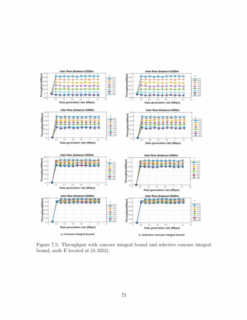
Data generation rate (Mbps)0 0.2 0.4 0.6 0.8 1 1.2 1.4
Th
rou
gh
pu
t(M
bp
s)
0.08
0.1
0.12
0.14
0.16
0.18
0.2inter-flow distance=2300m
0.20.30.40.50.60.70.80.9
Data generation rate (Mbps)0 0.2 0.4 0.6 0.8 1 1.2 1.4
Th
rou
gh
pu
t(M
bp
s)
0.08
0.1
0.12
0.14
0.16
0.18
0.2inter-flow distance=2300m
0.20.30.40.50.60.70.80.9
Data generation rate (Mbps)0 0.2 0.4 0.6 0.8 1 1.2 1.4
Th
rou
gh
pu
t(M
bp
s)
0.1
0.12
0.14
0.16
0.18
0.2
0.22inter-flow distance=2400m
0.20.30.40.50.60.70.80.9
Data generation rate (Mbps)0 0.2 0.4 0.6 0.8 1 1.2 1.4
Th
rou
gh
pu
t(M
bp
s)
0.1
0.12
0.14
0.16
0.18
0.2
0.22inter-flow distance=2400m
0.20.30.40.50.60.70.80.9
p p
pp
Data generation rate (Mbps)0 0.2 0.4 0.6 0.8 1 1.2 1.4
Th
rou
gh
pu
t(M
bp
s)
0.1
0.12
0.14
0.16
0.18
0.2
0.22inter-flow distance=2500m
0.20.30.40.50.60.70.80.9
Data generation rate (Mbps)0 0.2 0.4 0.6 0.8 1 1.2 1.4
Th
rou
gh
pu
t(M
bp
s)
0.1
0.12
0.14
0.16
0.18
0.2
0.22inter-flow distance=2500m
0.20.30.40.50.60.70.80.9
Data generation rate (Mbps)
a. Concave integral bound
0 0.2 0.4 0.6 0.8 1 1.2 1.4
Th
rou
gh
pu
t(M
bp
s)
0.1
0.12
0.14
0.16
0.18
0.2
0.22inter-flow distance=2600m
0.20.30.40.50.60.70.80.9
Data generation rate (Mbps)
b. Selective concave integral bound
0 0.2 0.4 0.6 0.8 1 1.2 1.4
Th
rou
gh
pu
t(M
bp
s)
0.1
0.12
0.14
0.16
0.18
0.2
0.22inter-flow distance=2600m
0.20.30.40.50.60.70.80.9
pp
pp
Figure 7.5: Throughput with concave integral bound and selective concave integralbound, node E located at (0, 3352).
73
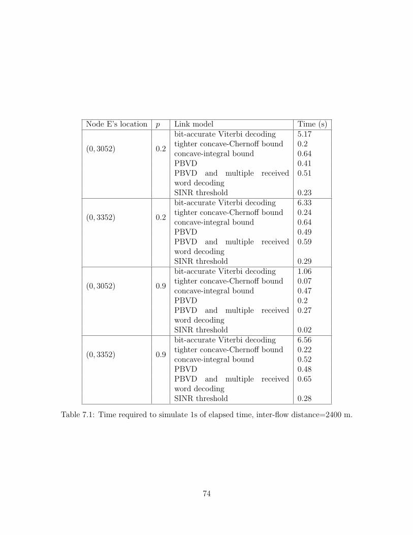
Node E’s location p Link model Time (s)
(0, 3052) 0.2
bit-accurate Viterbi decoding 5.17tighter concave-Chernoff bound 0.2concave-integral bound 0.64PBVD 0.41PBVD and multiple receivedword decoding
0.51
SINR threshold 0.23
(0, 3352) 0.2
bit-accurate Viterbi decoding 6.33tighter concave-Chernoff bound 0.24concave-integral bound 0.64PBVD 0.49PBVD and multiple receivedword decoding
0.59
SINR threshold 0.29
(0, 3052) 0.9
bit-accurate Viterbi decoding 1.06tighter concave-Chernoff bound 0.07concave-integral bound 0.47PBVD 0.2PBVD and multiple receivedword decoding
0.27
SINR threshold 0.02
(0, 3352) 0.9
bit-accurate Viterbi decoding 6.56tighter concave-Chernoff bound 0.22concave-integral bound 0.52PBVD 0.48PBVD and multiple receivedword decoding
0.65
SINR threshold 0.28
Table 7.1: Time required to simulate 1s of elapsed time, inter-flow distance=2400 m.
74
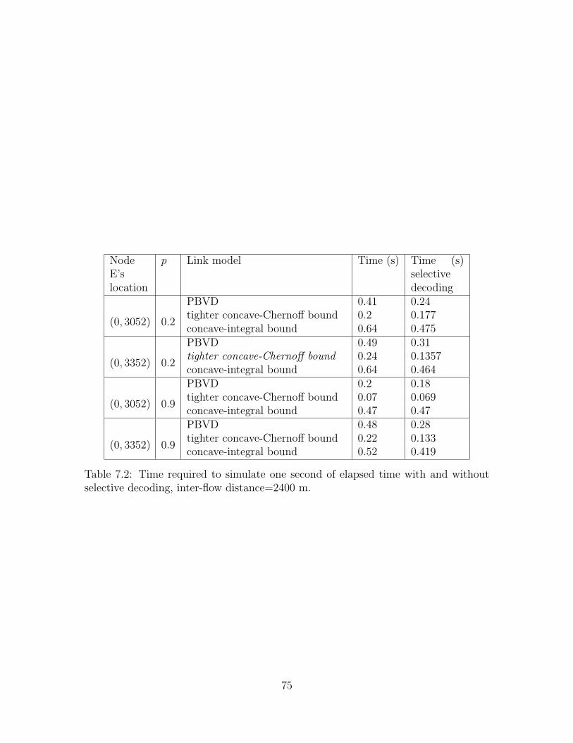
NodeE’slocation
p Link model Time (s) Time (s)selectivedecoding
(0, 3052) 0.2
PBVD 0.41 0.24tighter concave-Chernoff bound 0.2 0.177concave-integral bound 0.64 0.475
(0, 3352) 0.2
PBVD 0.49 0.31tighter concave-Chernoff bound 0.24 0.1357concave-integral bound 0.64 0.464
(0, 3052) 0.9
PBVD 0.2 0.18tighter concave-Chernoff bound 0.07 0.069concave-integral bound 0.47 0.47
(0, 3352) 0.9
PBVD 0.48 0.28tighter concave-Chernoff bound 0.22 0.133concave-integral bound 0.52 0.419
Table 7.2: Time required to simulate one second of elapsed time with and withoutselective decoding, inter-flow distance=2400 m.
75
Chapter 8
Link Modeling in Large-Network
Simulation
The small network considered in the examples in the previous chapters is a
convenient tool for providing insights into the tradeoffs of the different link models
for network simulation. A wireless ad hoc network of practical interest is likely to
have many more than four nodes, however, and it will require multiple-hop routing
in many instances. In this chapter, the comparison of link models introduced in the
previous chapters is extended to an example of a network of more realistic scale: the
large network described in Chapter 3.
Bit-accurate simulation of Viterbi decoding is again used as the benchmark
link model with respect to the results of the network simulation (that is, the through-
put measured in the simulation). As seen in Table 5.2, however, the CPU used for the
numerical results can require up to seven seconds to simulate one second of network
activity even for the small network with convolutional coding and on-line bit-accurate
Viterbi decoding. And depending on the network topology and the data flow, the
simulation time may increase more than linearly with the size of the network. Conse-
76
quently, off-line tabular modeling is used for bit-accurate Viterbi decoding with the
large network. (As seen in Chapter 4, this does not impact the simulated through-
put of the network.) A fine-resolution lookup table for each packet size used in the
network is constructed before the network simulation.
The measured throughput and the simulation time are compared for link mod-
els using off-line bit-accurate Viterbi decoding, the PBVD algorithm with selective
decoding in the network simulation, the two closed-form bounds on the probability
of code-word error, and the SINR threshold.
8.1 Simulation performance with the various link
models
The simulated network performance and the simulation time are considered in
this section for each of the data-flow scenarios indicated in Table 3.1. Performance
in each case is measured as the end-to-end throughput of the multiple-hop flow de-
noted as the main flow. The traffic in the main flow is subjected to multiple-access
interference from other nodes with a level of interference per interfering node given
by the interference activity probability.
The throughput for the topology in which the minimum-hop route for the
main flow is three hops is shown in Figure 8.1 as a function of the interference activ-
ity probability q for each of six values of the inter-node distance in the vertical axis
of the network topology. It is given for each of five link models. For a given vertical
distance, the throughput for the simulation with bit-accurate Viterbi decoding de-
creases towards a limiting value as q is increased. The throughput also decreases with
an increase in the vertical distance if q is fixed. If q = 0 (no interference), for exam-
77
ple, the throughput decreases from 0.1 Mpbs to 0.07 Mpbs as the vertical distance is
increased from 1300 m to 1350 m. If q = 1 (maximum interference), the throughput
decreases from 0.08 Mbps to 0.04 Mbps with the same increase in distance. The sim-
ulation using the PBVD algorithm with selective decoding results in a throughput
that is almost the same as the throughput with bit-accurate Viterbi decoding, which
is consistent with the results observed with the small network. (For the smallest
vertical distances only, selective decoding results in a modest overestimation of the
throughput.) This indicates that selective decoding can be used in the simulation of
a large network without significantly affecting the simulated network performance.
The throughput of the simulations using either of the two closed-form bounds
as the link model show a similar dependency on q and the vertical distance as occurs
with bit-accurate Viterbi decoding. As seen in Figure 8.1, if the vertical distance is less
than 1310 m, the throughput obtained using one of the bounds is approximately the
same as that with bit-accurate Viterbi decoding. But for a greater vertical distance,
either bound results in a significant underestimation of the throughput. Figure 8.1
also shows the throughput if the simulation employs a threshold-based link model with
an SINR threshold of γ = 3 dB. The threshold-based model results in a significant
overestimation of the throughput unless the vertical distance and the interference
activity factor are large. The throughput with the SINR threshold is almost twice
that with bit-accurate Viterbi decoding if the vertical distance is 1340 m and the
interferers are always active. A larger value of the SINR threshold would improve
the match with bit-accurate Viterbi decoding for the smaller vertical distances, but it
would exacerbate the underestimation with the threshold method for larger vertical
distances.
Similar results are observed in figures 8.2 and 8.3, which show the throughput
of the main flow spanning for circumstances in which the minimum-hop route for
78
the main flow is four hops and five hops, respectively. The simulation using selective
decoding with the PBVD algorithm results in throughput identical to the simulation
with bit-accurate Viterbi decoding in all instances. The use of either closed-form
bound for the link model results in an underestimation of the throughput that be-
comes more marked as the vertical distance is increased. The simulation using the
SINR threshold results in a significant overestimation of the throughput if the vertical
distance is small and a significant underestimation of the throughput if the vertical
distance is large.
The time required to simulate one second of network activity is shown in
Table 8.1 with each of the five link models for the network topology in which the
main flow spans a minimum of four hops. As the interference activity probability
q is increased from zero to one, the throughput in the main flow decreases with
each link model. But the total number of packets transmitted (and received) is
increased due to the increasing level of activity among the interfering nodes and
received at all nodes in the network so that the simulation time with each link model
increases substantially. For example, the simulation time with bit-accurate Viterbi
decoding increases approximately four-fold as the level of interference increases from
its minimum to its maximum value, for either vertical distance considered in the
table.
The simulation time with bit-accurate Viterbi decoding and the tighter concave-
Chernoff bound are nearly the same, though the comparison does not account for the
off-line simulation time required to build the look-up table for the former model. The
simulation time using the SINR threshold model is greater than with either of the
previous two models if the vertical distance is small (and the link SINRs are large),
and it is less than with either of the previous two models if the vertical distance is
large (and the link SINRs are small). This is a consequence of the simulation with
79
the SINR threshold generating more packet transmissions per unit time than with the
bit-accurate model if the link SINRs are large, and conversely if the link SINRs are
small (as also reflected in their relative measured throughputs). The simulation time
with the concave-integral bound is approximately three to four times the simulation
time with bit-accurate Viterbi decoding in each instance.
The simulation with selective decoding and the PBVD algorithm has a sim-
ulation time that is similar to that with bit-accurate Viterbi decoding. If there is
no interference (q = 0) so that the network activity is at a minimum, the simulation
time is approximately 15% greater with selective decoding and PBVD than with bit-
accurate Viterbi decoding. But if q = 1 so that the network is at its maximum level
of activity, the selective decoding eliminates the need to simulate decoding for a large
fraction of the packet reception attempts in the network. Hence, it results in a 5-20%
smaller simulation time than with bit-accurate Viterbi decoding.
80
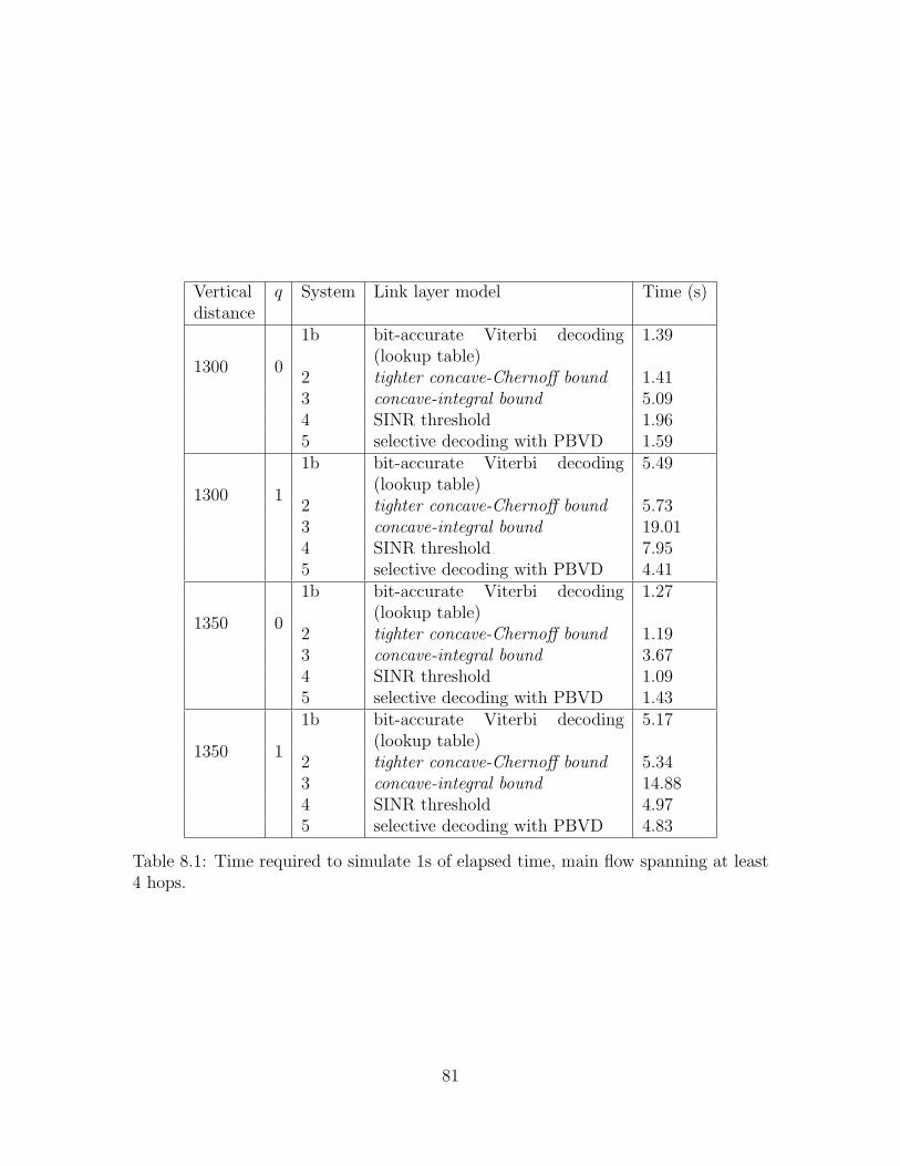
Verticaldistance
q System Link layer model Time (s)
1300 0
1b bit-accurate Viterbi decoding(lookup table)
1.39
2 tighter concave-Chernoff bound 1.413 concave-integral bound 5.094 SINR threshold 1.965 selective decoding with PBVD 1.59
1300 1
1b bit-accurate Viterbi decoding(lookup table)
5.49
2 tighter concave-Chernoff bound 5.733 concave-integral bound 19.014 SINR threshold 7.955 selective decoding with PBVD 4.41
1350 0
1b bit-accurate Viterbi decoding(lookup table)
1.27
2 tighter concave-Chernoff bound 1.193 concave-integral bound 3.674 SINR threshold 1.095 selective decoding with PBVD 1.43
1350 1
1b bit-accurate Viterbi decoding(lookup table)
5.17
2 tighter concave-Chernoff bound 5.343 concave-integral bound 14.884 SINR threshold 4.975 selective decoding with PBVD 4.83
Table 8.1: Time required to simulate 1s of elapsed time, main flow spanning at least4 hops.
81
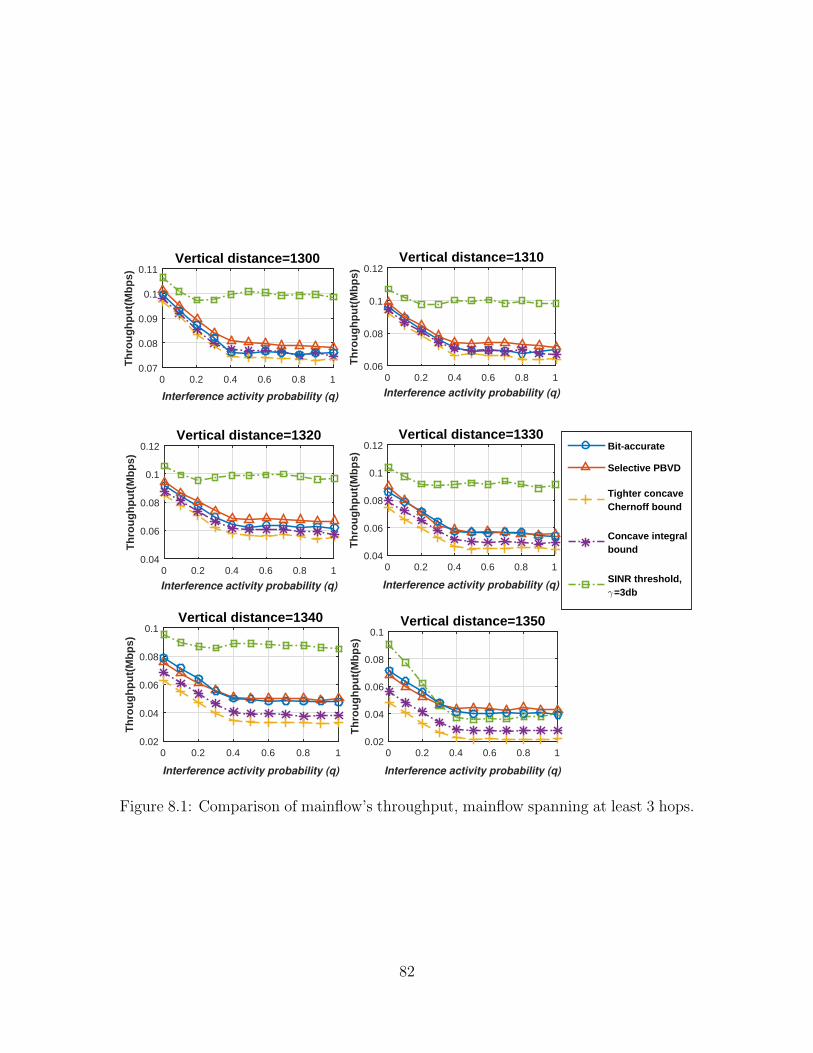
Interference activity probability (q)
0 0.2 0.4 0.6 0.8 1
Th
rou
gh
pu
t(M
bp
s)
0.07
0.08
0.09
0.1
0.11Vertical distance=1300
Interference activity probability (q)
0 0.2 0.4 0.6 0.8 1
Th
rou
gh
pu
t(M
bp
s)0.06
0.08
0.1
0.12Vertical distance=1310
Interference activity probability (q)
0 0.2 0.4 0.6 0.8 1
Th
rou
gh
pu
t(M
bp
s)
0.04
0.06
0.08
0.1
0.12Vertical distance=1320
Interference activity probability (q)
0 0.2 0.4 0.6 0.8 1
Th
rou
gh
pu
t(M
bp
s)
0.04
0.06
0.08
0.1
0.12Vertical distance=1330
Bit-accurate
Selective PBVD
Tighter concaveChernoff bound
Concave integralbound
SINR threshold,γ=3db
Interference activity probability (q)
0 0.2 0.4 0.6 0.8 1
Th
rou
gh
pu
t(M
bp
s)
0.02
0.04
0.06
0.08
0.1Vertical distance=1340
Interference activity probability (q)
0 0.2 0.4 0.6 0.8 1
Th
rou
gh
pu
t(M
bp
s)
0.02
0.04
0.06
0.08
0.1Vertical distance=1350
Figure 8.1: Comparison of mainflow’s throughput, mainflow spanning at least 3 hops.
82
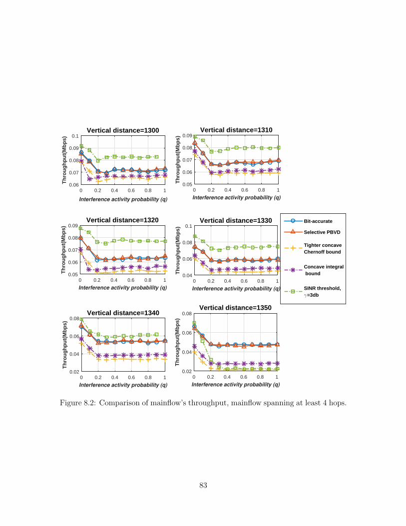
Interference activity probability (q)
0 0.2 0.4 0.6 0.8 1
Th
rou
gh
pu
t(M
bp
s)
0.06
0.07
0.08
0.09
0.1Vertical distance=1300
Interference activity probability (q)
0 0.2 0.4 0.6 0.8 1
Th
rou
gh
pu
t(M
bp
s)0.05
0.06
0.07
0.08
0.09Vertical distance=1310
Interference activity probability (q)
0 0.2 0.4 0.6 0.8 1
Th
rou
gh
pu
t(M
bp
s)
0.05
0.06
0.07
0.08
0.09Vertical distance=1320
Interference activity probability (q)
0 0.2 0.4 0.6 0.8 1
Th
rou
gh
pu
t(M
bp
s)
0.04
0.06
0.08
0.1Vertical distance=1330 Bit-accurate
Selective PBVD
Tighter concaveChernoff bound
Concave integral bound
SINR threshold,γ=3db
Interference activity probability (q)
0 0.2 0.4 0.6 0.8 1
Th
rou
gh
pu
t(M
bp
s)
0.02
0.04
0.06
0.08Vertical distance=1340
Interference activity probability (q)
0 0.2 0.4 0.6 0.8 1
Th
rou
gh
pu
t(M
bp
s)
0.02
0.04
0.06
0.08Vertical distance=1350
Figure 8.2: Comparison of mainflow’s throughput, mainflow spanning at least 4 hops.
83
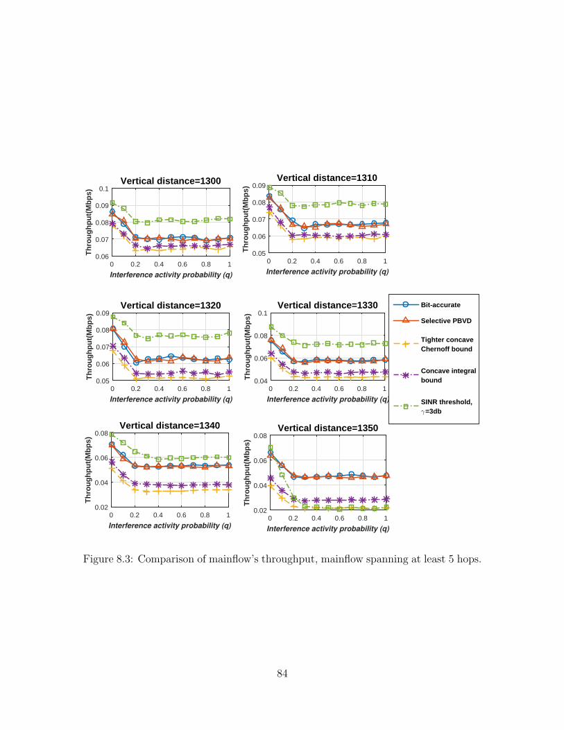
Interference activity probability (q)
0 0.2 0.4 0.6 0.8 1
Th
rou
gh
pu
t(M
bp
s)
0.06
0.07
0.08
0.09
0.1Vertical distance=1300
Interference activity probability (q)
0 0.2 0.4 0.6 0.8 1
Th
rou
gh
pu
t(M
bp
s)0.05
0.06
0.07
0.08
0.09Vertical distance=1310
Interference activity probability (q)
0 0.2 0.4 0.6 0.8 1
Th
rou
gh
pu
t(M
bp
s)
0.05
0.06
0.07
0.08
0.09Vertical distance=1320
Interference activity probability (q)
0 0.2 0.4 0.6 0.8 1
Th
rou
gh
pu
t(M
bp
s)
0.04
0.06
0.08
0.1Vertical distance=1330 Bit-accurate
Selective PBVD
Tighter concaveChernoff bound
Concave integralbound
SINR threshold,γ=3db
Interference activity probability (q)
0 0.2 0.4 0.6 0.8 1
Th
rou
gh
pu
t(M
bp
s)
0.02
0.04
0.06
0.08Vertical distance=1340
Interference activity probability (q)
0 0.2 0.4 0.6 0.8 1
Th
rou
gh
pu
t(M
bp
s)
0.02
0.04
0.06
0.08Vertical distance=1350
Figure 8.3: Comparison of mainflow’s throughput, mainflow spanning at least 5 hops.
84
Chapter 9
GPU-Based TDMP Decoding for
LDPC codes
Low density parity check (LDPC) codes are a class of linear block codes that
can achieve performance close to the Shannon capacity on an additive white Gaussian
noise channel for large block lengths. They provide very good performance in a wide
range of channels without the use of interleavers. Because of their performance, they
are widely used in modern communication systems. In this chapter, we consider the
GPU implementation of a decoding algorithm for a widely used example of an LDPC
code, the (2304,1152) quasi-cyclic (QC) LDPC defined in the WiMax standard, and
the turbo decoding message passing (TDMP) algorithm. The structure of a quasi-
cyclic LDPC and the form of the TDMP algorithm are well suited to exploit the
parallelism available in a GPU.
85
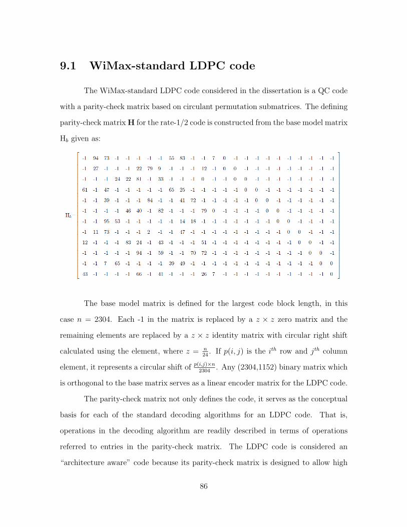
9.1 WiMax-standard LDPC code
The WiMax-standard LDPC code considered in the dissertation is a QC code
with a parity-check matrix based on circulant permutation submatrices. The defining
parity-check matrixH for the rate-1/2 code is constructed from the base model matrix
Hb given as:
The base model matrix is defined for the largest code block length, in this
case n = 2304. Each -1 in the matrix is replaced by a z × z zero matrix and the
remaining elements are replaced by a z × z identity matrix with circular right shift
calculated using the element, where z = n24. If p(i, j) is the ith row and jth column
element, it represents a circular shift of p(i,j)×n2304
. Any (2304,1152) binary matrix which
is orthogonal to the base matrix serves as a linear encoder matrix for the LDPC code.
The parity-check matrix not only defines the code, it serves as the conceptual
basis for each of the standard decoding algorithms for an LDPC code. That is,
operations in the decoding algorithm are readily described in terms of operations
referred to entries in the parity-check matrix. The LDPC code is considered an
“architecture aware” code because its parity-check matrix is designed to allow high
86
level of parallelism for decoding. If the rows of the base model matrix are arranged
in the order [0, 2, 4, 11, 6, 8, 10, 1, 3, 5, 7, 9], two consecutive rows do not intersect.
Thus, each code generated from the base matrix can be divided into 6 sets of rows
with each set containing 2 × z rows with disjoint sets of variable nodes, allowing all
the calculations on such rows to be done in parallel.
9.2 TDMP algorithm
The turbo decoding message passing (TDMP) algorithm [18] can be used to
efficiently decode the received word for any LDPC code defined by a sparse parity-
check matrix. In each iteration of the TDMP algorithm, updates of posterior values
for variable nodes are performed in a block-sequential manner. Extrinsic messages
generated from decoding earlier row blocks are used as input prior messages for
updates of the posterior value for variable nodes participating in later row blocks.
In the TDMP algorithm described below, the vector λi = [λi1, . . . , λ
ici] represents the
extrinsic messages that correspond to the nonzero entries in row i of parity-check
matrix H, where ci represents the row weight of row i. The notation Ii denotes
a list of the column positions of non-zero entries in row i in H. The vector γ =
[γ1, ..., γN ] represents the N posterior values, one for each code symbol vi. The subset
of the posterior messages corresponding to the non-zero column positions of row i are
denoted γ(Ii).
The algorithm is implemented as follows:
1. Initialize λi = 0, for i = 1, ...,M . Also, initialize the posterior values γ = [ri, ..., rn],
where ri is the real-valued channel output for vi. Each entry in γ is applied to a
uniform quantizer with quantization interval ∆ (and clipping) for subsequent fixed-
point processing using a signed, 8-bit representation.
87
2. Read the extrinsic messages λi and the posterior values γ(Ii) for row i.
3. Subtract λi from γ(Ii) to generate prior messages ρ = [ρ1, ..., ρci ] = γ(Ii)− λ(Ii)
4. Decode the parity-check equation for row i. Define α = [α1, ..., αci ] and β =
[β1, ..., βci ], where αj = sgn[ρj] (the sign of ρj) and βj = |ρj|. Set
λij =
(ci∏
k=1,k =j
αk
).max
(min
1≤k≤ci,k =jβk − η, 0
)
for j = 1, ..., ci, where the offset η is a non-negative constant that is an integer multiple
of the quantization interval. (The values of ∆ and η are chosen jointly to minimize
the error probability at some operating point of interest.)
5. Limit the maximum extrinsic updates in Step 4 to
λij = sgn
[λij
].min
(|λi
j|, ϵ)
where ϵ is a predetermined constant that is used to limit saturation in the posteriors.
It is also an integer multiple of the quantization interval.
6. Update the posterior values for the code-symbol positions of Ii as γ(Ii) = ρ+ λi.
7. Repeat the steps 2-6 for each row of H.
Steps 2-6 in the algorithm above are a decoding sub-iteration that updates the poste-
rior messages γ(Ii) corresponding to row i of H. In a single iteration, γ(Ii) is updated
for each row of H. The TDMP decoder goes through a fixed number of iterations in
an attempt to decode a received word. At the end of the fixed number of iterations a
parity-check decides if the received word is successfully decoded or not. If the decoded
word fails a parity check, a decoder failure is declared. A variation of the TDMP al-
gorithm performs parity-checks after each iteration and stops the decoding process
if the decoded word satisfies all the parity checks. However, a maximum number of
88
iterations is allowed and a decoder failure is declared if the decoded word fails a parity
check for each iteration through the maximum number of iterations. This variation of
the TDMP algorithm is referred to as the early terminating TDMP algorithm and the
original TDMP algorithm is referred to as the regular TDMP algorithm for discussion
purposes.
When executing the TDMP algorithm on a CPU, the sub-iteration of steps
2-6 are executed sequentially for the rows of H. If a GPU is used instead, the sub-
iteration can be carried out in parallel for the set of rows that contain disjoint sets
of variable nodes. Multiple received words can also be decoded in parallel if using a
GPU.
9.3 Implementing the TDMP algorithm on a GPU
TDMP decoding of QC-LDPC codes based on circular permutation sub matri-
ces is fitting to be implemented on GPUs as the computations on all the disjoint rows
can be carried out in parallel. Furthermore, multiple received words can be decoded
in parallel by assigning a separate grid of threads for each received word decoded in
parallel. Each thread in a block is responsible for computations for a set of rows that
do not have disjoint variable nodes. The computation for these disjoint rows must be
performed sequentially.
The TDMP algorithm requires only three large data arrays, namely γ, λi and
ρ for each row. For faster memory access when using GPUs, all the three variables
can be stored in shared memory. Unlike the Viterbi decoder, the GPU’s shared
memory is sufficient to store all three variables for the TDMP algorithm. Another
large array that contains the location of the non-zero elements in the H matrix is
stored in constant memory as it is a read-only data.
89
TheWiMax standard, (2304,1152) LDPC code used in the network simulations
has 6 sets of rows with each set containing 192 rows with disjoint variable nodes. Thus,
192 threads are launched with each thread being responsible for calculations of 6 rows.
The calculations for the 6 rows are carried out serially.
If the regular TDMP algorithm is implemented, each thread carries out a pre-
determined maximum number of iterations before determining if the received word
has been decoded to a valid code word (i.e., the decoder output satisfies all the
parity checks for the code). If early termination is used with the TDMP algorithm,
however, a single thread in each block performs all parity checks after each iteration
and stores the result in a variable shared by the entire block. All the threads in a
block (corresponding to one received word) stop the decoding process if the variable
indicates that the parity checks are successful. The blocks corresponding to other
received words that haven’t passed the parity checks continue on with the decoding
process if multiple received words are being decoded in parallel.
9.4 Performance evaluation of TDMP algorithm
using CPU and GPU
The performance of the TDMP algorithm using a CPU and a GPU is compared
by considering a system that consists of a single transmitting node and a single
receiving node. An Intel Xeon E5-2665, 2.4 GHz processor is used for the CPU
simulations and a 16-core 2.7 GHz Intel Zeon E5-2680 CPU with two NVIDIA TESLA
k40 GPUs is used for the GPU simulations. Parallel decoding of multiple received
words is implemented in the GPU. For each value of the SNR, the simulation is
carried out till 1000 packets are decoded in error at the receiver. A maximum of 50
90
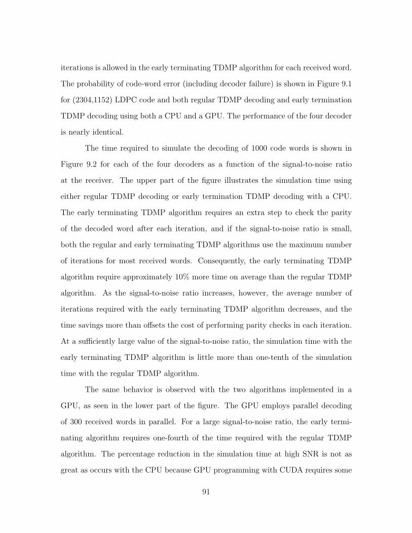
iterations is allowed in the early terminating TDMP algorithm for each received word.
The probability of code-word error (including decoder failure) is shown in Figure 9.1
for (2304,1152) LDPC code and both regular TDMP decoding and early termination
TDMP decoding using both a CPU and a GPU. The performance of the four decoder
is nearly identical.
The time required to simulate the decoding of 1000 code words is shown in
Figure 9.2 for each of the four decoders as a function of the signal-to-noise ratio
at the receiver. The upper part of the figure illustrates the simulation time using
either regular TDMP decoding or early termination TDMP decoding with a CPU.
The early terminating TDMP algorithm requires an extra step to check the parity
of the decoded word after each iteration, and if the signal-to-noise ratio is small,
both the regular and early terminating TDMP algorithms use the maximum number
of iterations for most received words. Consequently, the early terminating TDMP
algorithm require approximately 10% more time on average than the regular TDMP
algorithm. As the signal-to-noise ratio increases, however, the average number of
iterations required with the early terminating TDMP algorithm decreases, and the
time savings more than offsets the cost of performing parity checks in each iteration.
At a sufficiently large value of the signal-to-noise ratio, the simulation time with the
early terminating TDMP algorithm is little more than one-tenth of the simulation
time with the regular TDMP algorithm.
The same behavior is observed with the two algorithms implemented in a
GPU, as seen in the lower part of the figure. The GPU employs parallel decoding
of 300 received words in parallel. For a large signal-to-noise ratio, the early termi-
nating algorithm requires one-fourth of the time required with the regular TDMP
algorithm. The percentage reduction in the simulation time at high SNR is not as
great as occurs with the CPU because GPU programming with CUDA requires some
91
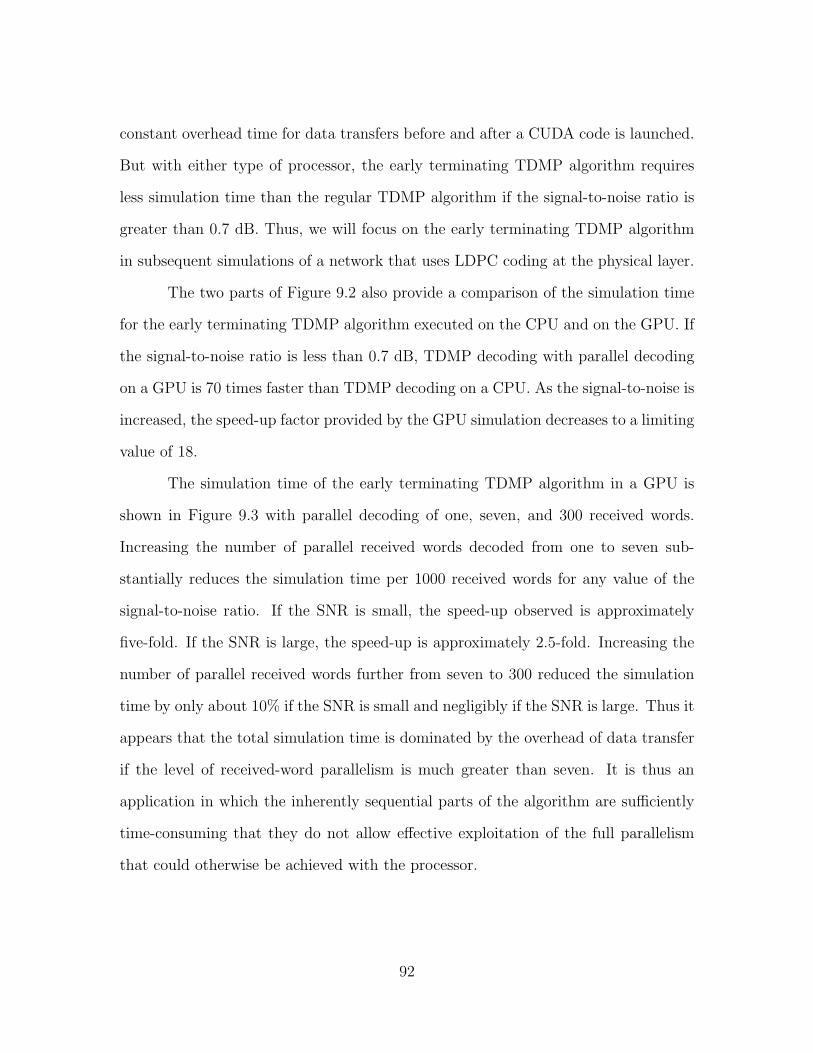
constant overhead time for data transfers before and after a CUDA code is launched.
But with either type of processor, the early terminating TDMP algorithm requires
less simulation time than the regular TDMP algorithm if the signal-to-noise ratio is
greater than 0.7 dB. Thus, we will focus on the early terminating TDMP algorithm
in subsequent simulations of a network that uses LDPC coding at the physical layer.
The two parts of Figure 9.2 also provide a comparison of the simulation time
for the early terminating TDMP algorithm executed on the CPU and on the GPU. If
the signal-to-noise ratio is less than 0.7 dB, TDMP decoding with parallel decoding
on a GPU is 70 times faster than TDMP decoding on a CPU. As the signal-to-noise is
increased, the speed-up factor provided by the GPU simulation decreases to a limiting
value of 18.
The simulation time of the early terminating TDMP algorithm in a GPU is
shown in Figure 9.3 with parallel decoding of one, seven, and 300 received words.
Increasing the number of parallel received words decoded from one to seven sub-
stantially reduces the simulation time per 1000 received words for any value of the
signal-to-noise ratio. If the SNR is small, the speed-up observed is approximately
five-fold. If the SNR is large, the speed-up is approximately 2.5-fold. Increasing the
number of parallel received words further from seven to 300 reduced the simulation
time by only about 10% if the SNR is small and negligibly if the SNR is large. Thus it
appears that the total simulation time is dominated by the overhead of data transfer
if the level of received-word parallelism is much greater than seven. It is thus an
application in which the inherently sequential parts of the algorithm are sufficiently
time-consuming that they do not allow effective exploitation of the full parallelism
that could otherwise be achieved with the processor.
92
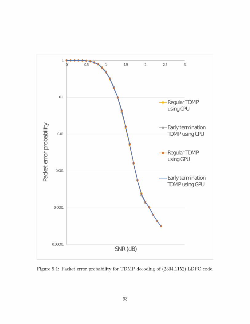
0.00001
0.0001
0.001
0.01
0.1
1
0 0.5 1 1.5 2 2.5 3
Pac
ket err
or pro
bab
ility
SNR (dB)
Regular TDMP
using CPU
Early termination
TDMP using CPU
Regular TDMP
using GPU
Early termination
TDMP using GPU
Figure 9.1: Packet error probability for TDMP decoding of (2304,1152) LDPC code.
93
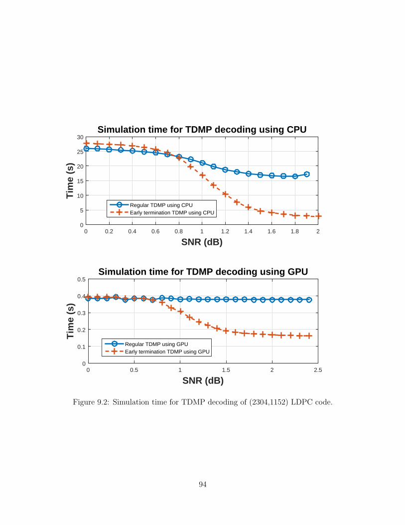
SNR (dB)0 0.2 0.4 0.6 0.8 1 1.2 1.4 1.6 1.8 2
Tim
e (s
)
0
5
10
15
20
25
30Simulation time for TDMP decoding using CPU
Regular TDMP using CPUEarly termination TDMP using CPU
SNR (dB)0 0.5 1 1.5 2 2.5
Tim
e (s
)
0
0.1
0.2
0.3
0.4
0.5Simulation time for TDMP decoding using GPU
Regular TDMP using GPUEarly termination TDMP using GPU
Figure 9.2: Simulation time for TDMP decoding of (2304,1152) LDPC code.
94
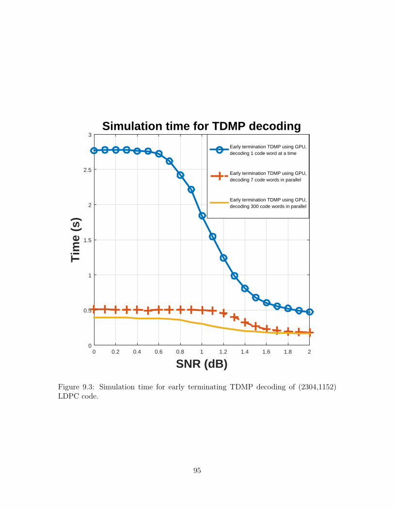
SNR (dB)0 0.2 0.4 0.6 0.8 1 1.2 1.4 1.6 1.8 2
Tim
e (s
)
0
0.5
1
1.5
2
2.5
3Simulation time for TDMP decoding
Early termination TDMP using GPU,decoding 1 code word at a time
Early termination TDMP using GPU,decoding 7 code words in parallel
Early termination TDMP using GPU,decoding 300 code words in parallel
Figure 9.3: Simulation time for early terminating TDMP decoding of (2304,1152)LDPC code.
95
Chapter 10
Network Simulation with
GPU-Accelerated TDMP Decoding
In this chapter, we consider simulations of an ad hoc radio network (imple-
mented in ns-3) in which each link uses LDPC coding and TDMP decoding for data
packet transmissions. The throughput and simulation times are compared for CPU
implementation and GPU implementation of bit-accurate TDMP decoding as well as
with a link model using an SINR threshold. Both the small network and the large
network are considered.
Each link uses the (2304,1152) WiMax LDPC code and TDMP decoding with
early termination for data packet transmissions, and each data packet contains seven
code words transmitted consecutively on the channel. Each control packet is encoded
as a single code word of the rate-1/2 NASA-standard convolutional and is detected
using Viterbi decoding. The time-varying interference at the receiver over the du-
ration of the packet transmission is modeled by the equivalent stationary Gaussian
noise channel for both data packets and control packets.
If the GPU is used for decoding, the seven received words corresponding to a
96
single data packet are decoded in parallel but decoding for different packets occurs
sequentially. A decoder failure for one or more code words is treated as a packet
detection failure. Each control packet contains a single convolutional code word, and
decoding for different control packets on GPU occurs sequentially. Selective decoding
is also used with the GPU so that decoding is not actually implemented for packets
that are overheard by third-party receivers.
10.1 Simulation of the small network with TDMP
decoding
The throughput of flow 1 of the small network is shown in Figure 10.1 if
the interfering node is located at position (0,3052) for several values of the inter-
flow distance between 1900 m and 2200 m and different values of the interference
probability p. Both simulation using a CPU and simulation using a GPU for TDMP
decoding are considered. It is seen that the type of processor used has little effect
on the simulated throughput. The throughput obtained with bit-accurate TDMP
decoding is compared with the throughput obtained with a SINR threshold link model
in Figures 10.2 and 10.3 for values of the SINR threshold of γ = 1.5 dB and γ = 1.6
dB, respectively.
The use of the SINR threshold results in simulation results with much greater
sensitivity to the network parameters than does the bit-accurate link model of TDMP
decoding. The sensitivity is particularly great in conditions of heavy interference, as
seen in the figures if the interference probability p = 0.9. The simulated throughput is
almost zero with a threshold of 1.5 dB if the inter-flow distance is 1900 m (so that the
SINR of the link is small during many link transmissions), and it under-estimates the
97
0.05 Mbps throughput obtained with the bit-accurate model. In contrast, the SINR
threshold results in a modest over-estimation of the 0.21 Mbps simulated throughput
with the bit-accurate model if the inter-flow distance is large (so that the SINR is
larger during most link transmissions). A similar pattern is observed in Figure 10.6
with an SINR threshold of 1.6 dB. Similar observations also result from Figures 10.4,
10.5 and 10.6 which show the throughput of flow 1 if the interfering node is located
at position (0,3352) for values of the inter-flow distance between 1500 m and 1800 m.
Comparison of the results from the six figures indicates that an SINR threshold
of 1.5 dB results in a somewhat better approximation to the bit-accurate performance
overall. Any change in the SINR threshold results in a trade-off between the fidelity
of the model in conditions resulting in high SINR links and the fidelity of the model in
conditions resulting in low SINR links. Comparison with the results in Chapter 4 also
indicate that the inaccuracies inherent in the SINR threshold model are less significant
in the network using the LDPC code than in the network using the convolutional
code for data packets. This is explained by considering the “waterfall curve” of the
probability of code-word error as a function of the SINR in a white Gaussian noise
channel for the two link coding methods.The LDPC code with TDMP decoding has
a steeper waterfall curve than does the convolutional code with Viterbi decoding so
that the behavior of the former more nearly exhibits an SINR threshold effect than
does the behavior of the latter.
The time required to simulate one second of network activity is shown in Table
10.1 for each of the link models. The interfering node is located at position (0,3052) if
the inter-flow distance is 1900 m and it is located at position (0,3352) if the inter-flow
distance is 1800 m in the examples. The simulation time for the small network with
early termination TDMP decoding implemented on a CPU requires more than one
second to simulate one second of network activity, whereas on a GPU it requires only
98
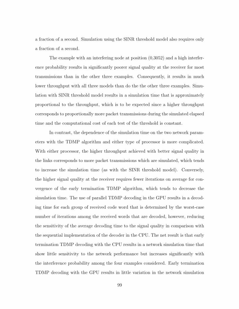
a fraction of a second. Simulation using the SINR threshold model also requires only
a fraction of a second.
The example with an interfering node at position (0,3052) and a high interfer-
ence probability results in significantly poorer signal quality at the receiver for most
transmissions than in the other three examples. Consequently, it results in much
lower throughput with all three models than do the the other three examples. Simu-
lation with SINR threshold model results in a simulation time that is approximately
proportional to the throughput, which is to be expected since a higher throughput
corresponds to proportionally more packet transmissions during the simulated elapsed
time and the computational cost of each test of the threshold is constant.
In contrast, the dependence of the simulation time on the two network param-
eters with the TDMP algorithm and either type of processor is more complicated.
With either processor, the higher throughput achieved with better signal quality in
the links corresponds to more packet transmissions which are simulated, which tends
to increase the simulation time (as with the SINR threshold model). Conversely,
the higher signal quality at the receiver requires fewer iterations on average for con-
vergence of the early termination TDMP algorithm, which tends to decrease the
simulation time. The use of parallel TDMP decoding in the GPU results in a decod-
ing time for each group of received code word that is determined by the worst-case
number of iterations among the received words that are decoded, however, reducing
the sensitivity of the average decoding time to the signal quality in comparison with
the sequential implementation of the decoder in the CPU. The net result is that early
termination TDMP decoding with the CPU results in a network simulation time that
show little sensitivity to the network performance but increases significantly with
the interference probability among the four examples considered. Early termination
TDMP decoding with the GPU results in little variation in the network simulation
99
time among the four examples.
10.2 Simulation of the large network with TDMP
decoding
The three link models are also considered in a simulation of the 64-node large
network in which the vertical distance between adjacent nodes is fixed at 1600 m and
the horizontal distance between adjacent nodes is varied from 1500 m to 1550 m. The
network performance is measured as the throughput for the main flow as defined in
Chapter 3 for each of three network topologies and traffic scenarios. In the examples
considered, the other network flows are located such that their channel reservation
(RTS/CTS) exchanges have a negligible effect on link transmission opportunities for
the main flow, though they can result in significant multiple-access interference at
the receiver for transmissions in each link of the main flow.
On-line implementation of early terminating TDMP decoding on the CPU
is replaced by a table look-up model on the CPU decoding in order to limit the
simulation time with the model. The look-up table is generated from off-line bit-
accurate simulation of the probability of code-word error indexed by the average
SINR over the code word. The model is tested by considering its accuracy in the
small network as shown in Figures 10.7 and 10.8, which show the throughput for flow
1 of the small network with both on-line early termination TDMP decoding on a
CPU and the off-line table look-up model. Two locations for the interfering node are
considered in the examples. As seen in figure 10.7 and 10.8, the throughput with the
two models differs negligibly.
The simulated throughput in the main flow is shown in Figure 10.9 for the
100
network topology main flow spanning at least three hops. The throughput with bit-
accurate early termination TDMP decoding implemented on either type of processor
is greatest if the interference activity probability q = 0 (that is, if the interfering flows
are never active). The throughput decreases slightly as the interference probability is
increased to one (so that the interfering flows are always active). The use of the SINR
threshold model with γ = 1.8 dB yields very different simulation results, however. For
each horizontal distance less than 1550 m that is considered, the SINR at the receiver
of each node in the main flow is greater than the threshold γ; thus, the model indicates
that each packet transmission is detected correctly and no link transmission errors
are reflected in the model. The throughput with the SINR threshold model is greater
than 0.95 Mbps, and it is much greater than that obtained with the bit-accurate
model, regardless of the value of q.
If the horizontal distance is 1550 m, in contrast, the SINR at each receiver in
the main flow is close to the threshold γ if no interferers are active. As a result, if q =
0, there is a substantive throughput in the flow with the model. As the interference
in the network increases with an increasing value of q, however, the received SINR
at each receiver on the main flow falls below the threshold with increasing frequency
so that the flow exhibits little throughput with the model. The throughput with the
SINR threshold model is 0.05 Mbps if q = 0 and decreases to almost zero as q is
increased to one. This is well below the throughput obtained with the bit-accurate
model. Changing the threshold results in a tradeoff between the fidelity of the model
for a small horizontal distance and its fidelity for a large horizontal distance.
The throughput of the main flow in the network topology in which the main
flow spans at least four hops is shown in Figure 10.10, and its throughput in the
topology in which the main flow spans at least five hops is shown in Figure 10.11. As
seen in the previous examples, the throughput with the bit-accurate TDMP algorithm
101

differs negligibly depending on the type of processor used to implement it. The
throughput decreases as the interference activity probability q is increased for each
value of the horizontal distance. And as seen in the previous examples, the use of the
SINR threshold model in the network simulation results in an over-estimation of the
throughput if the horizontal distance is small, and it results in an under-estimation
of the throughput if the horizontal distance is large.
The time required to simulate one second of network activity is shown in Table
10.2. The simulation times for the three link models do not differ dramatically for a
given value of the horizontal distance and a given value of the interference activity
probability. The simulation time with the SINR threshold model is smaller than with
table look-up for bit-accurate TDMP decoding, however. The table look-up model
requires one table for each of the packet sizes used in the network. With the latter
link model, the network simulation must determine the correct table to use and then
read from the table for each link transmission simulated, whereas with the SINR
threshold model only a simple test is required. As the value of q is increased from
zero to one, interfering flows become more active in the network, which results in
the transmission of more packets in the network. Consequently, the simulation time
increases also four-fold as q is increased from zero to one with each of the three link
models.
102
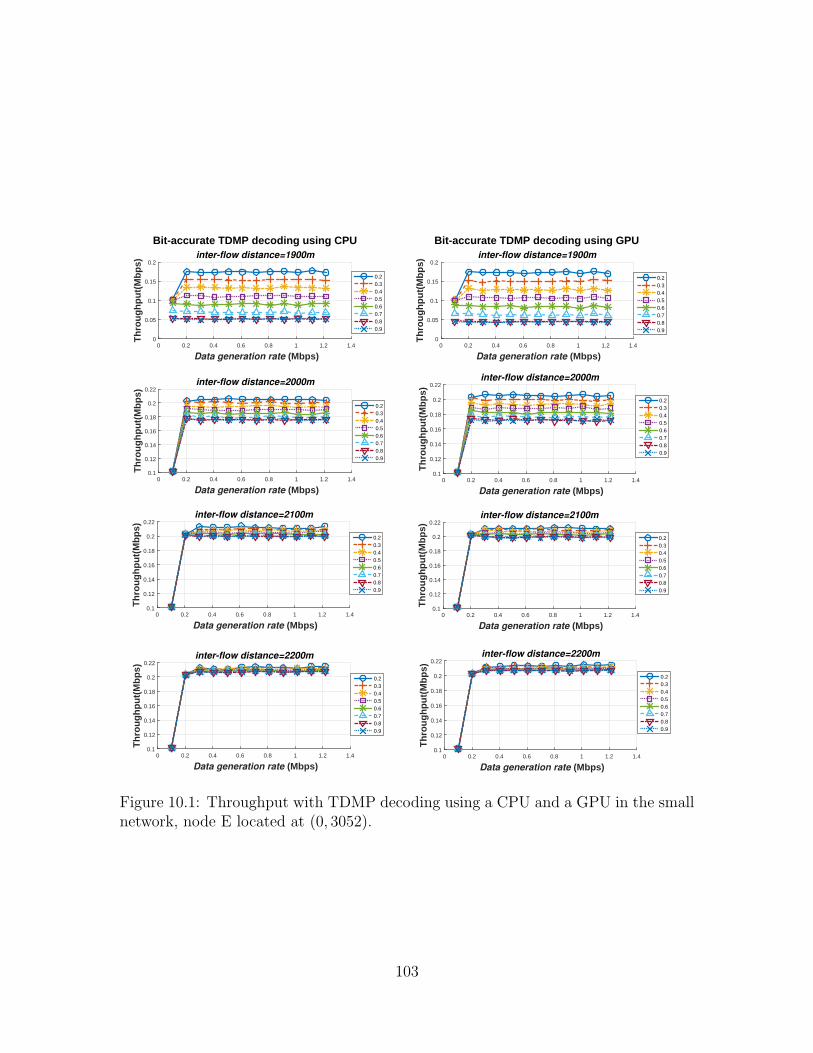
Data generation rate (Mbps)0 0.2 0.4 0.6 0.8 1 1.2 1.4
Th
rou
gh
pu
t(M
bp
s)
0
0.05
0.1
0.15
0.2
Bit-accurate TDMP decoding using CPUinter-flow distance=1900m
0.20.30.40.50.60.70.80.9
Data generation rate (Mbps)0 0.2 0.4 0.6 0.8 1 1.2 1.4
Th
rou
gh
pu
t(M
bp
s)
0
0.05
0.1
0.15
0.2
Bit-accurate TDMP decoding using GPUinter-flow distance=1900m
0.20.30.40.50.60.70.80.9
Data generation rate (Mbps)0 0.2 0.4 0.6 0.8 1 1.2 1.4
Th
rou
gh
pu
t(M
bp
s)
0.1
0.12
0.14
0.16
0.18
0.2
0.22inter-flow distance=2000m
0.20.30.40.50.60.70.80.9
Data generation rate (Mbps)0 0.2 0.4 0.6 0.8 1 1.2 1.4
Th
rou
gh
pu
t(M
bp
s)
0.1
0.12
0.14
0.16
0.18
0.2
0.22inter-flow distance=2000m
0.20.30.40.50.60.70.80.9
Data generation rate (Mbps)0 0.2 0.4 0.6 0.8 1 1.2 1.4
Th
rou
gh
pu
t(M
bp
s)
0.1
0.12
0.14
0.16
0.18
0.2
0.22inter-flow distance=2100m
0.20.30.40.50.60.70.80.9
Data generation rate (Mbps)0 0.2 0.4 0.6 0.8 1 1.2 1.4
Th
rou
gh
pu
t(M
bp
s)
0.1
0.12
0.14
0.16
0.18
0.2
0.22inter-flow distance=2100m
0.20.30.40.50.60.70.80.9
Data generation rate (Mbps)0 0.2 0.4 0.6 0.8 1 1.2 1.4
Th
rou
gh
pu
t(M
bp
s)
0.1
0.12
0.14
0.16
0.18
0.2
0.22inter-flow distance=2200m
0.20.30.40.50.60.70.80.9
Data generation rate (Mbps)0 0.2 0.4 0.6 0.8 1 1.2 1.4
Th
rou
gh
pu
t(M
bp
s)
0.1
0.12
0.14
0.16
0.18
0.2
0.22inter-flow distance=2200m
0.20.30.40.50.60.70.80.9
Figure 10.1: Throughput with TDMP decoding using a CPU and a GPU in the smallnetwork, node E located at (0, 3052).
103
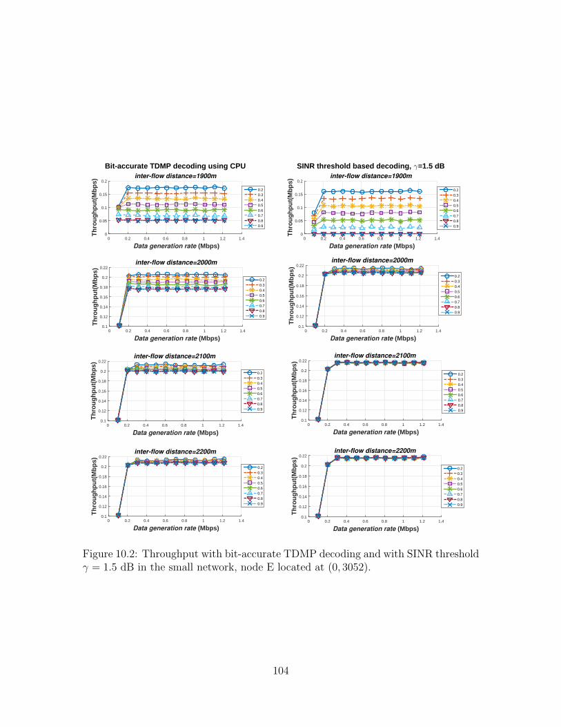
Data generation rate (Mbps)0 0.2 0.4 0.6 0.8 1 1.2 1.4
Th
rou
gh
pu
t(M
bp
s)
0
0.05
0.1
0.15
0.2
Bit-accurate TDMP decoding using CPUinter-flow distance=1900m
0.20.30.40.50.60.70.80.9
Data generation rate (Mbps)0 0.2 0.4 0.6 0.8 1 1.2 1.4
Th
rou
gh
pu
t(M
bp
s)
0
0.05
0.1
0.15
0.2
SINR threshold based decoding, γ=1.5 dBinter-flow distance=1900m
0.20.30.40.50.60.70.80.9
Data generation rate (Mbps)0 0.2 0.4 0.6 0.8 1 1.2 1.4
Th
rou
gh
pu
t(M
bp
s)
0.1
0.12
0.14
0.16
0.18
0.2
0.22inter-flow distance=2000m
0.20.30.40.50.60.70.80.9
Data generation rate (Mbps)0 0.2 0.4 0.6 0.8 1 1.2 1.4
Th
rou
gh
pu
t(M
bp
s)
0.1
0.12
0.14
0.16
0.18
0.2
0.22inter-flow distance=2000m
0.20.30.40.50.60.70.80.9
Data generation rate (Mbps)0 0.2 0.4 0.6 0.8 1 1.2 1.4
Th
rou
gh
pu
t(M
bp
s)
0.1
0.12
0.14
0.16
0.18
0.2
0.22inter-flow distance=2100m
0.20.30.40.50.60.70.80.9
Data generation rate (Mbps)0 0.2 0.4 0.6 0.8 1 1.2 1.4
Th
rou
gh
pu
t(M
bp
s)
0.1
0.12
0.14
0.16
0.18
0.2
0.22inter-flow distance=2100m
0.20.30.40.50.60.70.80.9
Data generation rate (Mbps)0 0.2 0.4 0.6 0.8 1 1.2 1.4
Th
rou
gh
pu
t(M
bp
s)
0.1
0.12
0.14
0.16
0.18
0.2
0.22inter-flow distance=2200m
0.20.30.40.50.60.70.80.9
Data generation rate (Mbps)0 0.2 0.4 0.6 0.8 1 1.2 1.4
Th
rou
gh
pu
t(M
bp
s)
0.1
0.12
0.14
0.16
0.18
0.2
0.22inter-flow distance=2200m
0.20.30.40.50.60.70.80.9
Figure 10.2: Throughput with bit-accurate TDMP decoding and with SINR thresholdγ = 1.5 dB in the small network, node E located at (0, 3052).
104
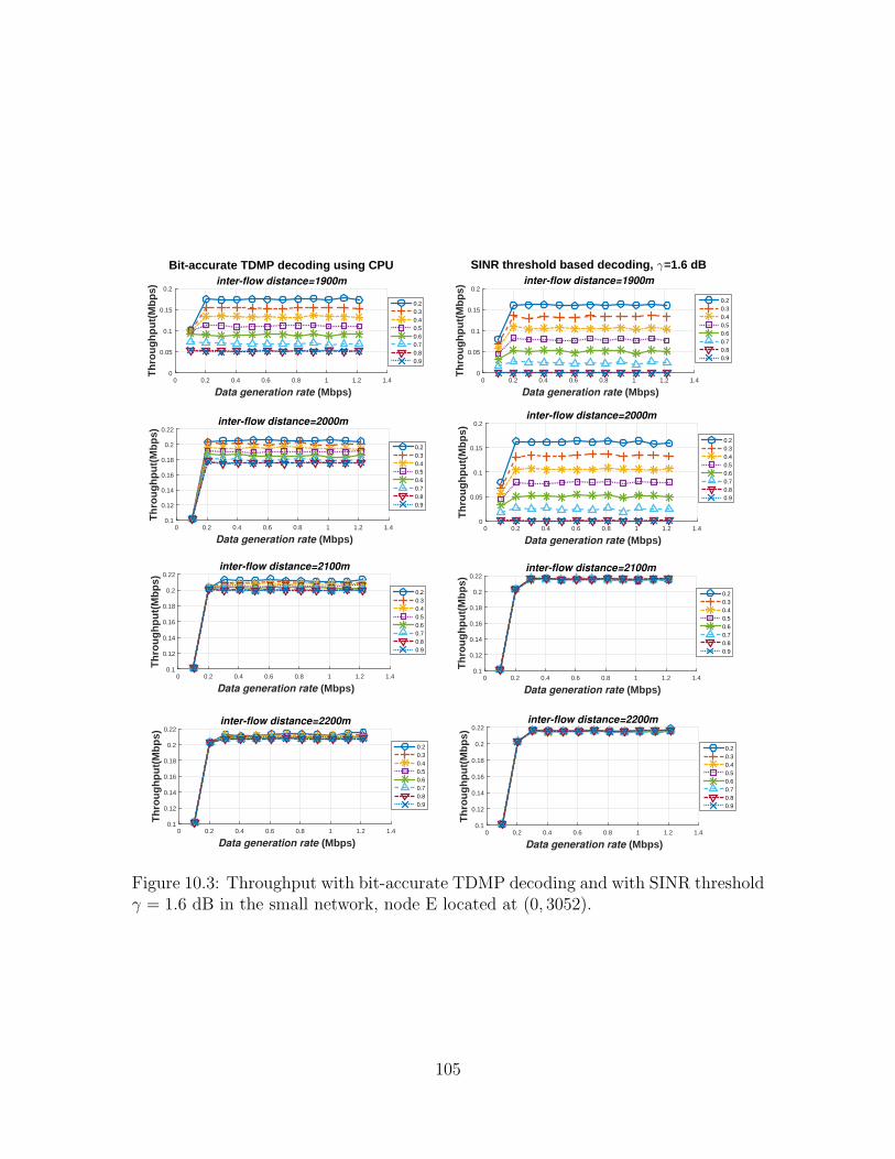
Data generation rate (Mbps)0 0.2 0.4 0.6 0.8 1 1.2 1.4
Th
rou
gh
pu
t(M
bp
s)
0
0.05
0.1
0.15
0.2
Bit-accurate TDMP decoding using CPUinter-flow distance=1900m
0.20.30.40.50.60.70.80.9
Data generation rate (Mbps)0 0.2 0.4 0.6 0.8 1 1.2 1.4
Th
rou
gh
pu
t(M
bp
s)
0
0.05
0.1
0.15
0.2
SINR threshold based decoding, γ=1.6 dBinter-flow distance=1900m
0.20.30.40.50.60.70.80.9
Data generation rate (Mbps)0 0.2 0.4 0.6 0.8 1 1.2 1.4
Th
rou
gh
pu
t(M
bp
s)
0.1
0.12
0.14
0.16
0.18
0.2
0.22inter-flow distance=2000m
0.20.30.40.50.60.70.80.9
Data generation rate (Mbps)0 0.2 0.4 0.6 0.8 1 1.2 1.4
Th
rou
gh
pu
t(M
bp
s)
0
0.05
0.1
0.15
0.2inter-flow distance=2000m
0.20.30.40.50.60.70.80.9
Data generation rate (Mbps)0 0.2 0.4 0.6 0.8 1 1.2 1.4
Th
rou
gh
pu
t(M
bp
s)
0.1
0.12
0.14
0.16
0.18
0.2
0.22inter-flow distance=2100m
0.20.30.40.50.60.70.80.9
Data generation rate (Mbps)0 0.2 0.4 0.6 0.8 1 1.2 1.4
Th
rou
gh
pu
t(M
bp
s)
0.1
0.12
0.14
0.16
0.18
0.2
0.22inter-flow distance=2100m
0.20.30.40.50.60.70.80.9
Data generation rate (Mbps)0 0.2 0.4 0.6 0.8 1 1.2 1.4
Th
rou
gh
pu
t(M
bp
s)
0.1
0.12
0.14
0.16
0.18
0.2
0.22inter-flow distance=2200m
0.20.30.40.50.60.70.80.9
Data generation rate (Mbps)0 0.2 0.4 0.6 0.8 1 1.2 1.4
Th
rou
gh
pu
t(M
bp
s)
0.1
0.12
0.14
0.16
0.18
0.2
0.22inter-flow distance=2200m
0.20.30.40.50.60.70.80.9
Figure 10.3: Throughput with bit-accurate TDMP decoding and with SINR thresholdγ = 1.6 dB in the small network, node E located at (0, 3052).
105
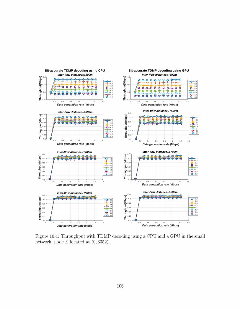
Data generation rate (Mbps)0 0.2 0.4 0.6 0.8 1 1.2 1.4
Th
rou
gh
pu
t(M
bp
s)
0.05
0.1
0.15
0.2
Bit-accurate TDMP decoding using CPUinter-flow distance=1500m
0.20.30.40.50.60.70.80.9
Data generation rate (Mbps)0 0.2 0.4 0.6 0.8 1 1.2 1.4
Th
rou
gh
pu
t(M
bp
s)
0.05
0.1
0.15
0.2
Bit-accurate TDMP decoding using GPU inter-flow distance=1500m
0.20.30.40.50.60.70.80.9
Data generation rate (Mbps)0 0.2 0.4 0.6 0.8 1 1.2 1.4
Th
rou
gh
pu
t(M
bp
s)
0.1
0.12
0.14
0.16
0.18
0.2
0.22inter-flow distance=1600m
0.20.30.40.50.60.70.80.9
Data generation rate (Mbps)0 0.2 0.4 0.6 0.8 1 1.2 1.4
Th
rou
gh
pu
t(M
bp
s)
0.1
0.12
0.14
0.16
0.18
0.2
0.22inter-flow distance=1600m
0.20.30.40.50.60.70.80.9
Data generation rate (Mbps)0 0.2 0.4 0.6 0.8 1 1.2 1.4
Th
rou
gh
pu
t(M
bp
s)
0.1
0.12
0.14
0.16
0.18
0.2
0.22inter-flow distance=1700m
0.20.30.40.50.60.70.80.9
Data generation rate (Mbps)0 0.2 0.4 0.6 0.8 1 1.2 1.4
Th
rou
gh
pu
t(M
bp
s)
0.1
0.12
0.14
0.16
0.18
0.2
0.22inter-flow distance=1700m
0.20.30.40.50.60.70.80.9
Data generation rate (Mbps)0 0.2 0.4 0.6 0.8 1 1.2 1.4
Th
rou
gh
pu
t(M
bp
s)
0.1
0.12
0.14
0.16
0.18
0.2
0.22inter-flow distance=1800m
0.20.30.40.50.60.70.80.9
Data generation rate (Mbps)0 0.2 0.4 0.6 0.8 1 1.2 1.4
Th
rou
gh
pu
t(M
bp
s)
0.1
0.12
0.14
0.16
0.18
0.2
0.22inter-flow distance=1800m
0.20.30.40.50.60.70.80.9
Figure 10.4: Throughput with TDMP decoding using a CPU and a GPU in the smallnetwork, node E located at (0, 3352).
106
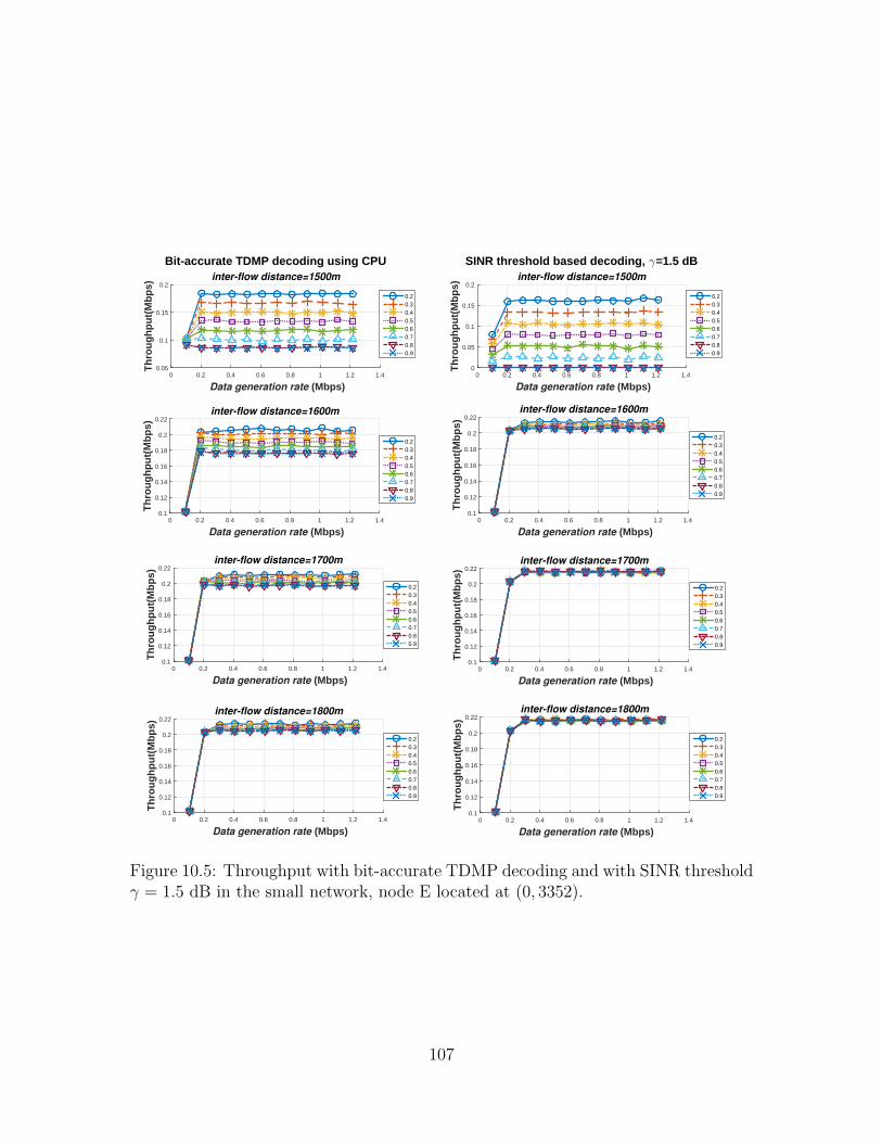
Data generation rate (Mbps)0 0.2 0.4 0.6 0.8 1 1.2 1.4
Th
rou
gh
pu
t(M
bp
s)
0.05
0.1
0.15
0.2
Bit-accurate TDMP decoding using CPUinter-flow distance=1500m
0.20.30.40.50.60.70.80.9
Data generation rate (Mbps)0 0.2 0.4 0.6 0.8 1 1.2 1.4
Th
rou
gh
pu
t(M
bp
s)
0
0.05
0.1
0.15
0.2
SINR threshold based decoding, γ=1.5 dBinter-flow distance=1500m
0.20.30.40.50.60.70.80.9
Data generation rate (Mbps)0 0.2 0.4 0.6 0.8 1 1.2 1.4
Th
rou
gh
pu
t(M
bp
s)
0.1
0.12
0.14
0.16
0.18
0.2
0.22inter-flow distance=1600m
0.20.30.40.50.60.70.80.9
Data generation rate (Mbps)0 0.2 0.4 0.6 0.8 1 1.2 1.4
Th
rou
gh
pu
t(M
bp
s)
0.1
0.12
0.14
0.16
0.18
0.2
0.22inter-flow distance=1600m
0.20.30.40.50.60.70.80.9
Data generation rate (Mbps)0 0.2 0.4 0.6 0.8 1 1.2 1.4
Th
rou
gh
pu
t(M
bp
s)
0.1
0.12
0.14
0.16
0.18
0.2
0.22inter-flow distance=1700m
0.20.30.40.50.60.70.80.9
Data generation rate (Mbps)0 0.2 0.4 0.6 0.8 1 1.2 1.4
Th
rou
gh
pu
t(M
bp
s)
0.1
0.12
0.14
0.16
0.18
0.2
0.22inter-flow distance=1700m
0.20.30.40.50.60.70.80.9
Data generation rate (Mbps)0 0.2 0.4 0.6 0.8 1 1.2 1.4
Th
rou
gh
pu
t(M
bp
s)
0.1
0.12
0.14
0.16
0.18
0.2
0.22inter-flow distance=1800m
0.20.30.40.50.60.70.80.9
Data generation rate (Mbps)0 0.2 0.4 0.6 0.8 1 1.2 1.4
Th
rou
gh
pu
t(M
bp
s)
0.1
0.12
0.14
0.16
0.18
0.2
0.22inter-flow distance=1800m
0.20.30.40.50.60.70.80.9
Figure 10.5: Throughput with bit-accurate TDMP decoding and with SINR thresholdγ = 1.5 dB in the small network, node E located at (0, 3352).
107
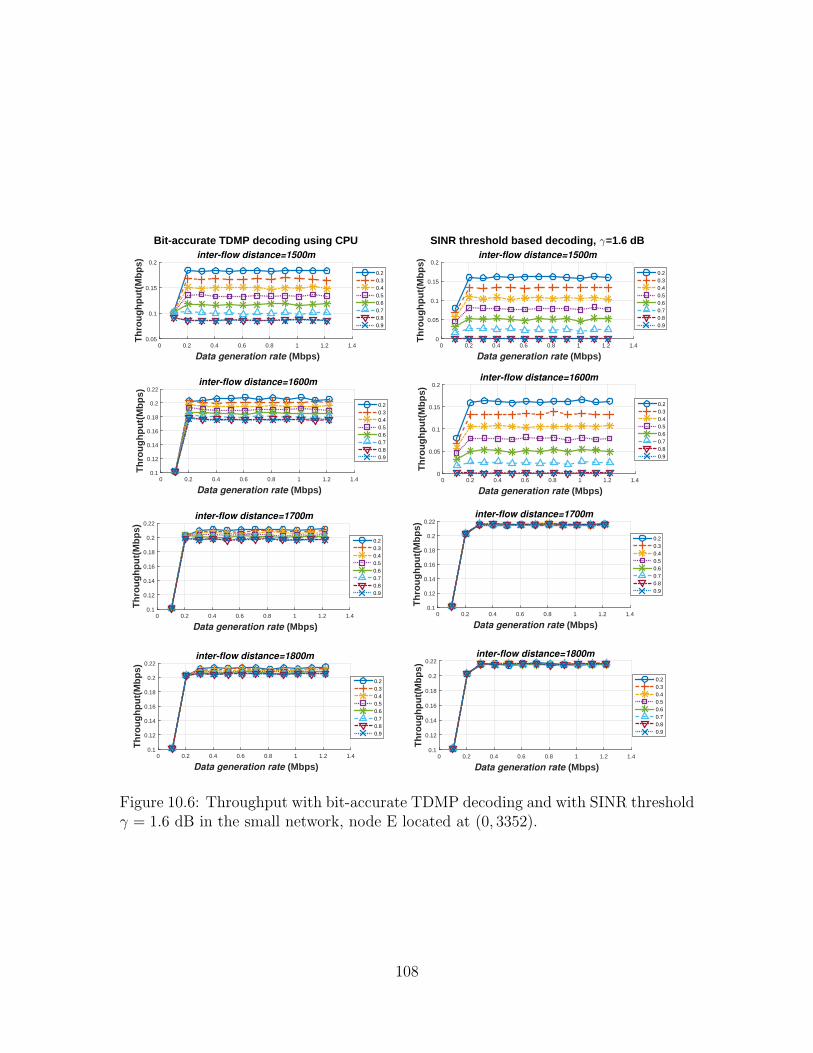
Data generation rate (Mbps)0 0.2 0.4 0.6 0.8 1 1.2 1.4
Th
rou
gh
pu
t(M
bp
s)
0.05
0.1
0.15
0.2
Bit-accurate TDMP decoding using CPUinter-flow distance=1500m
0.20.30.40.50.60.70.80.9
Data generation rate (Mbps)0 0.2 0.4 0.6 0.8 1 1.2 1.4
Th
rou
gh
pu
t(M
bp
s)
0
0.05
0.1
0.15
0.2
SINR threshold based decoding, γ=1.6 dBinter-flow distance=1500m
0.20.30.40.50.60.70.80.9
Data generation rate (Mbps)0 0.2 0.4 0.6 0.8 1 1.2 1.4
Th
rou
gh
pu
t(M
bp
s)
0.1
0.12
0.14
0.16
0.18
0.2
0.22inter-flow distance=1600m
0.20.30.40.50.60.70.80.9
Data generation rate (Mbps)0 0.2 0.4 0.6 0.8 1 1.2 1.4
Th
rou
gh
pu
t(M
bp
s)
0
0.05
0.1
0.15
0.2inter-flow distance=1600m
0.20.30.40.50.60.70.80.9
Data generation rate (Mbps)0 0.2 0.4 0.6 0.8 1 1.2 1.4
Th
rou
gh
pu
t(M
bp
s)
0.1
0.12
0.14
0.16
0.18
0.2
0.22inter-flow distance=1700m
0.20.30.40.50.60.70.80.9
Data generation rate (Mbps)0 0.2 0.4 0.6 0.8 1 1.2 1.4
Th
rou
gh
pu
t(M
bp
s)
0.1
0.12
0.14
0.16
0.18
0.2
0.22inter-flow distance=1700m
0.20.30.40.50.60.70.80.9
Data generation rate (Mbps)0 0.2 0.4 0.6 0.8 1 1.2 1.4
Th
rou
gh
pu
t(M
bp
s)
0.1
0.12
0.14
0.16
0.18
0.2
0.22inter-flow distance=1800m
0.20.30.40.50.60.70.80.9
Data generation rate (Mbps)0 0.2 0.4 0.6 0.8 1 1.2 1.4
Th
rou
gh
pu
t(M
bp
s)
0.1
0.12
0.14
0.16
0.18
0.2
0.22inter-flow distance=1800m
0.20.30.40.50.60.70.80.9
Figure 10.6: Throughput with bit-accurate TDMP decoding and with SINR thresholdγ = 1.6 dB in the small network, node E located at (0, 3352).
108
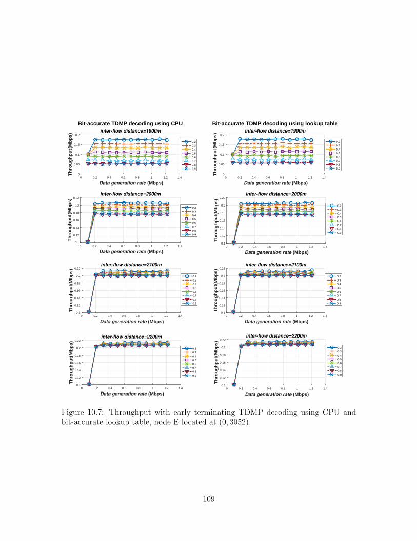
Data generation rate (Mbps)0 0.2 0.4 0.6 0.8 1 1.2 1.4
Th
rou
gh
pu
t(M
bp
s)
0
0.05
0.1
0.15
0.2
Bit-accurate TDMP decoding using CPUinter-flow distance=1900m
0.20.30.40.50.60.70.80.9
Data generation rate (Mbps)0 0.2 0.4 0.6 0.8 1 1.2 1.4
Th
rou
gh
pu
t(M
bp
s)
0
0.05
0.1
0.15
0.2
Bit-accurate TDMP decoding using lookup tableinter-flow distance=1900m
0.20.30.40.50.60.70.80.9
Data generation rate (Mbps)0 0.2 0.4 0.6 0.8 1 1.2 1.4
Th
rou
gh
pu
t(M
bp
s)
0.1
0.12
0.14
0.16
0.18
0.2
0.22inter-flow distance=2000m
0.20.30.40.50.60.70.80.9
Data generation rate (Mbps)0 0.2 0.4 0.6 0.8 1 1.2 1.4
Th
rou
gh
pu
t(M
bp
s)
0.1
0.12
0.14
0.16
0.18
0.2
0.22inter-flow distance=2000m
0.20.30.40.50.60.70.80.9
Data generation rate (Mbps)0 0.2 0.4 0.6 0.8 1 1.2 1.4
Th
rou
gh
pu
t(M
bp
s)
0.1
0.12
0.14
0.16
0.18
0.2
0.22inter-flow distance=2100m
0.20.30.40.50.60.70.80.9
Data generation rate (Mbps)0 0.2 0.4 0.6 0.8 1 1.2 1.4
Th
rou
gh
pu
t(M
bp
s)
0.1
0.12
0.14
0.16
0.18
0.2
0.22inter-flow distance=2100m
0.20.30.40.50.60.70.80.9
Data generation rate (Mbps)0 0.2 0.4 0.6 0.8 1 1.2 1.4
Th
rou
gh
pu
t(M
bp
s)
0.1
0.12
0.14
0.16
0.18
0.2
0.22inter-flow distance=2200m
0.20.30.40.50.60.70.80.9
Data generation rate (Mbps)0 0.2 0.4 0.6 0.8 1 1.2 1.4
Th
rou
gh
pu
t(M
bp
s)
0.1
0.12
0.14
0.16
0.18
0.2
0.22inter-flow distance=2200m
0.20.30.40.50.60.70.80.9
Figure 10.7: Throughput with early terminating TDMP decoding using CPU andbit-accurate lookup table, node E located at (0, 3052).
109
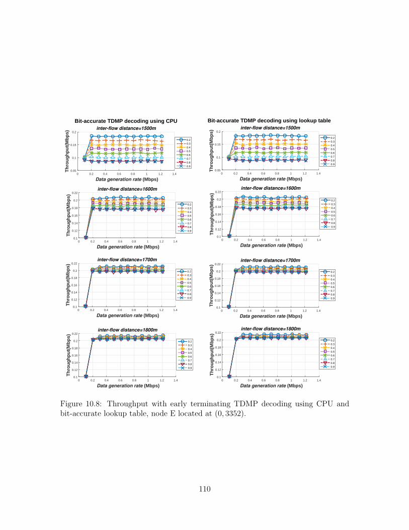
Data generation rate (Mbps)0 0.2 0.4 0.6 0.8 1 1.2 1.4
Th
rou
gh
pu
t(M
bp
s)
0.05
0.1
0.15
0.2
Bit-accurate TDMP decoding using CPUinter-flow distance=1500m
0.20.30.40.50.60.70.80.9
Data generation rate (Mbps)0 0.2 0.4 0.6 0.8 1 1.2 1.4
Th
rou
gh
pu
t(M
bp
s)
0.05
0.1
0.15
0.2
Bit-accurate TDMP decoding using lookup table inter-flow distance=1500m
0.20.30.40.50.60.70.80.9
Data generation rate (Mbps)0 0.2 0.4 0.6 0.8 1 1.2 1.4
Th
rou
gh
pu
t(M
bp
s)
0.1
0.12
0.14
0.16
0.18
0.2
0.22inter-flow distance=1600m
0.20.30.40.50.60.70.80.9
Data generation rate (Mbps)0 0.2 0.4 0.6 0.8 1 1.2 1.4
Th
rou
gh
pu
t(M
bp
s)
0.1
0.12
0.14
0.16
0.18
0.2
0.22inter-flow distance=1600m
0.20.30.40.50.60.70.80.9
Data generation rate (Mbps)0 0.2 0.4 0.6 0.8 1 1.2 1.4
Th
rou
gh
pu
t(M
bp
s)
0.1
0.12
0.14
0.16
0.18
0.2
0.22inter-flow distance=1700m
0.20.30.40.50.60.70.80.9
Data generation rate (Mbps)0 0.2 0.4 0.6 0.8 1 1.2 1.4
Th
rou
gh
pu
t(M
bp
s)
0.1
0.12
0.14
0.16
0.18
0.2
0.22inter-flow distance=1700m
0.20.30.40.50.60.70.80.9
Data generation rate (Mbps)0 0.2 0.4 0.6 0.8 1 1.2 1.4
Th
rou
gh
pu
t(M
bp
s)
0.1
0.12
0.14
0.16
0.18
0.2
0.22inter-flow distance=1800m
0.20.30.40.50.60.70.80.9
Data generation rate (Mbps)0 0.2 0.4 0.6 0.8 1 1.2 1.4
Th
rou
gh
pu
t(M
bp
s)
0.1
0.12
0.14
0.16
0.18
0.2
0.22inter-flow distance=1800m
0.20.30.40.50.60.70.80.9
Figure 10.8: Throughput with early terminating TDMP decoding using CPU andbit-accurate lookup table, node E located at (0, 3352).
110
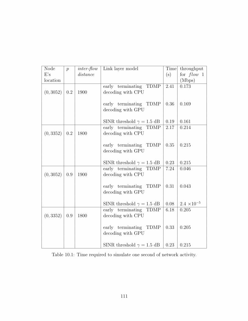
NodeE’slocation
p inter-flowdistance
Link layer model Time(s)
throughputfor flow 1(Mbps)
(0, 3052) 0.2 1900early terminating TDMPdecoding with CPU
2.41 0.173
early terminating TDMPdecoding with GPU
0.36 0.169
SINR threshold γ = 1.5 dB 0.19 0.161
(0, 3352) 0.2 1800early terminating TDMPdecoding with CPU
2.17 0.214
early terminating TDMPdecoding with GPU
0.35 0.215
SINR threshold γ = 1.5 dB 0.23 0.215
(0, 3052) 0.9 1900early terminating TDMPdecoding with CPU
7.24 0.046
early terminating TDMPdecoding with GPU
0.31 0.043
SINR threshold γ = 1.5 dB 0.08 2.4 ×10⁻⁵
(0, 3352) 0.9 1800early terminating TDMPdecoding with CPU
6.18 0.205
early terminating TDMPdecoding with GPU
0.33 0.205
SINR threshold γ = 1.5 dB 0.23 0.215
Table 10.1: Time required to simulate one second of network activity.
111
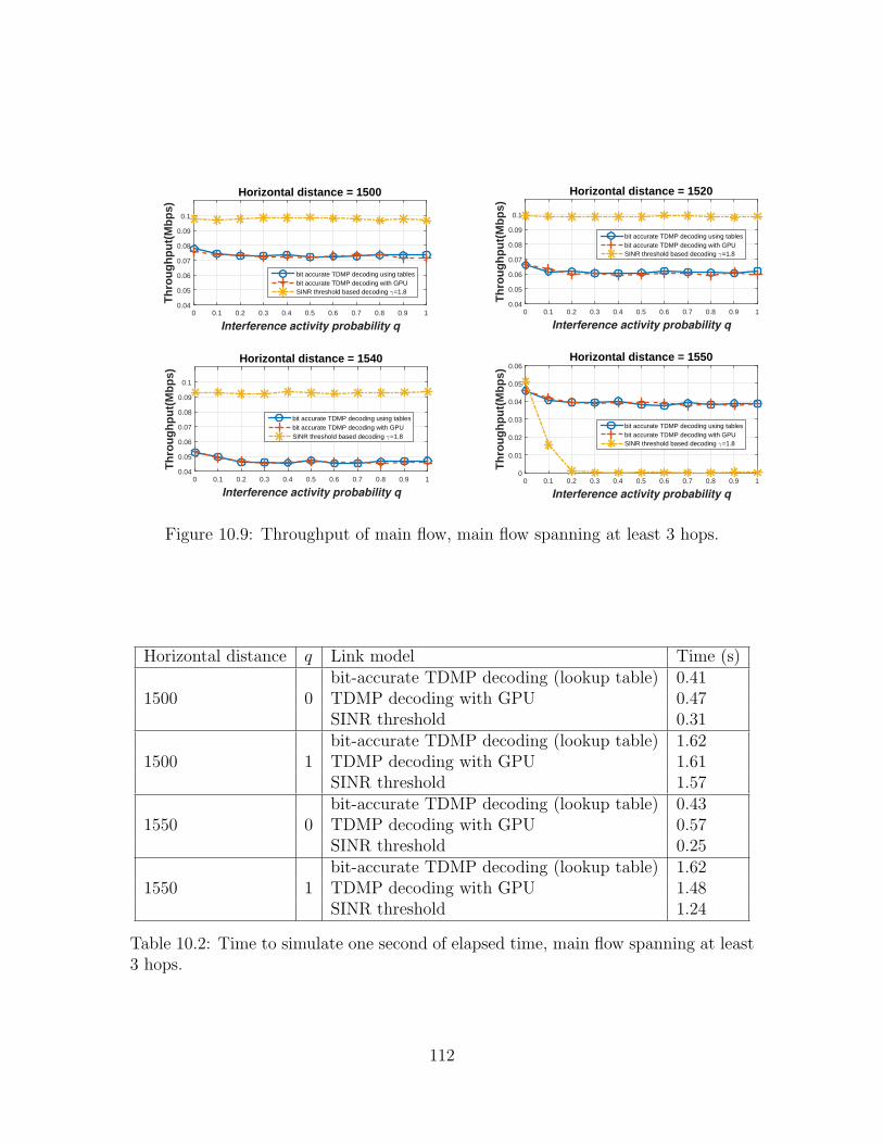
Interference activity probability q
0 0.1 0.2 0.3 0.4 0.5 0.6 0.7 0.8 0.9 1
Th
rou
gh
pu
t(M
bp
s)
0.04
0.05
0.06
0.07
0.08
0.09
0.1
Horizontal distance = 1500
bit accurate TDMP decoding using tablesbit accurate TDMP decoding with GPUSINR threshold based decoding γ=1.8
Interference activity probability q
0 0.1 0.2 0.3 0.4 0.5 0.6 0.7 0.8 0.9 1
Th
rou
gh
pu
t(M
bp
s)
0.04
0.05
0.06
0.07
0.08
0.09
0.1
Horizontal distance = 1520
bit accurate TDMP decoding using tablesbit accurate TDMP decoding with GPUSINR threshold based decoding γ=1.8
Interference activity probability q
0 0.1 0.2 0.3 0.4 0.5 0.6 0.7 0.8 0.9 1
Th
rou
gh
pu
t(M
bp
s)
0.04
0.05
0.06
0.07
0.08
0.09
0.1
Horizontal distance = 1540
bit accurate TDMP decoding using tablesbit accurate TDMP decoding with GPUSINR threshold based decoding γ=1.8
Interference activity probability q
0 0.1 0.2 0.3 0.4 0.5 0.6 0.7 0.8 0.9 1
Th
rou
gh
pu
t(M
bp
s)
0
0.01
0.02
0.03
0.04
0.05
0.06Horizontal distance = 1550
bit accurate TDMP decoding using tablesbit accurate TDMP decoding with GPUSINR threshold based decoding γ=1.8
Figure 10.9: Throughput of main flow, main flow spanning at least 3 hops.
Horizontal distance q Link model Time (s)
1500 0bit-accurate TDMP decoding (lookup table) 0.41TDMP decoding with GPU 0.47SINR threshold 0.31
1500 1bit-accurate TDMP decoding (lookup table) 1.62TDMP decoding with GPU 1.61SINR threshold 1.57
1550 0bit-accurate TDMP decoding (lookup table) 0.43TDMP decoding with GPU 0.57SINR threshold 0.25
1550 1bit-accurate TDMP decoding (lookup table) 1.62TDMP decoding with GPU 1.48SINR threshold 1.24
Table 10.2: Time to simulate one second of elapsed time, main flow spanning at least3 hops.
112
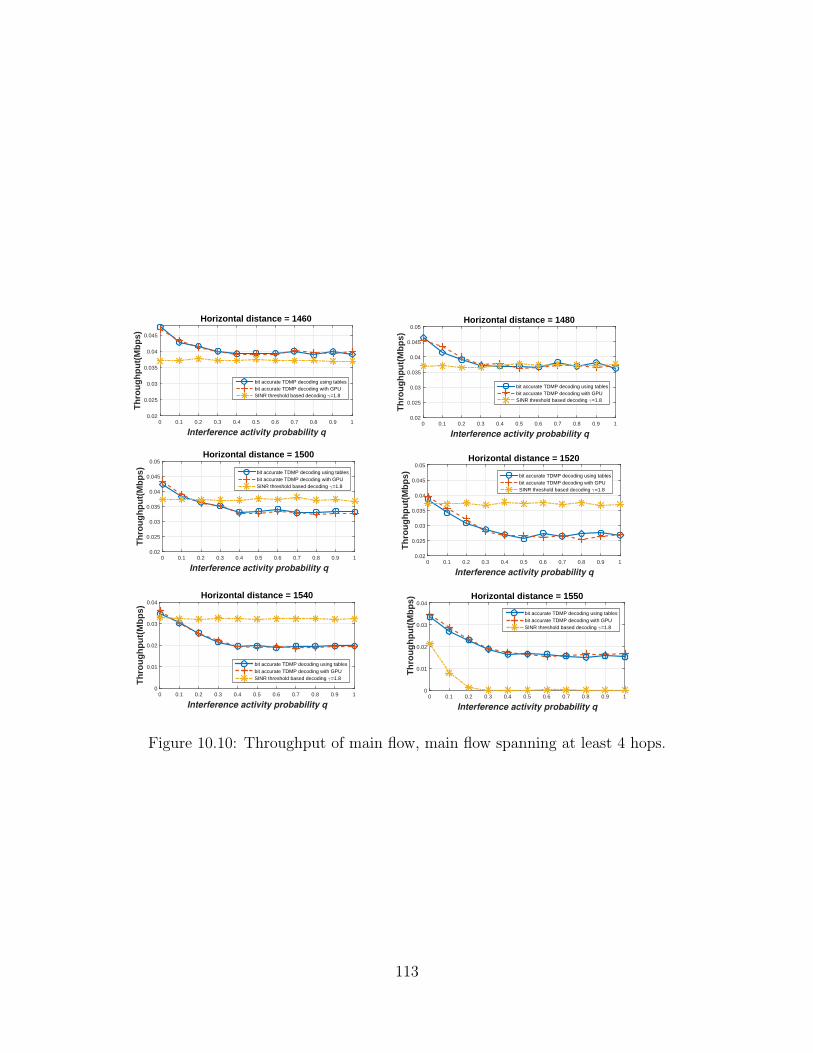
Interference activity probability q
0 0.1 0.2 0.3 0.4 0.5 0.6 0.7 0.8 0.9 1
Th
rou
gh
pu
t(M
bp
s)
0.02
0.025
0.03
0.035
0.04
0.045
Horizontal distance = 1460
bit accurate TDMP decoding using tablesbit accurate TDMP decoding with GPUSINR threshold based decoding γ=1.8
Interference activity probability q
0 0.1 0.2 0.3 0.4 0.5 0.6 0.7 0.8 0.9 1
Th
rou
gh
pu
t(M
bp
s)
0.02
0.025
0.03
0.035
0.04
0.045
0.05Horizontal distance = 1480
bit accurate TDMP decoding using tablesbit accurate TDMP decoding with GPUSINR threshold based decoding γ=1.8
Interference activity probability q
0 0.1 0.2 0.3 0.4 0.5 0.6 0.7 0.8 0.9 1
Th
rou
gh
pu
t(M
bp
s)
0.02
0.025
0.03
0.035
0.04
0.045
0.05Horizontal distance = 1500
bit accurate TDMP decoding using tablesbit accurate TDMP decoding with GPUSINR threshold based decoding γ=1.8
Interference activity probability q
0 0.1 0.2 0.3 0.4 0.5 0.6 0.7 0.8 0.9 1
Th
rou
gh
pu
t(M
bp
s)
0.02
0.025
0.03
0.035
0.04
0.045
0.05Horizontal distance = 1520
bit accurate TDMP decoding using tablesbit accurate TDMP decoding with GPUSINR threshold based decoding γ=1.8
Interference activity probability q
0 0.1 0.2 0.3 0.4 0.5 0.6 0.7 0.8 0.9 1
Th
rou
gh
pu
t(M
bp
s)
0
0.01
0.02
0.03
0.04Horizontal distance = 1540
bit accurate TDMP decoding using tablesbit accurate TDMP decoding with GPUSINR threshold based decoding γ=1.8
Interference activity probability q
0 0.1 0.2 0.3 0.4 0.5 0.6 0.7 0.8 0.9 1
Th
rou
gh
pu
t(M
bp
s)
0
0.01
0.02
0.03
0.04Horizontal distance = 1550
bit accurate TDMP decoding using tablesbit accurate TDMP decoding with GPUSINR threshold based decoding γ=1.8
Figure 10.10: Throughput of main flow, main flow spanning at least 4 hops.
113
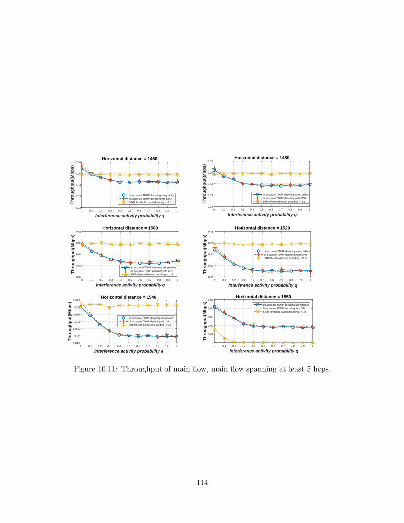
Interference activity probability q
0 0.1 0.2 0.3 0.4 0.5 0.6 0.7 0.8 0.9 1
Th
rou
gh
pu
t(M
bp
s)
0.02
0.03
0.04
0.05
0.06Horizontal distance = 1460
bit accurate TDMP decoding using tablesbit accurate TDMP decoding with GPUSINR threshold based decoding γ=1.8
Interference activity probability q
0 0.1 0.2 0.3 0.4 0.5 0.6 0.7 0.8 0.9 1
Th
rou
gh
pu
t(M
bp
s)0.02
0.03
0.04
0.05
0.06Horizontal distance = 1480
bit accurate TDMP decoding using tablesbit accurate TDMP decoding with GPUSINR threshold based decoding γ=1.8
Interference activity probability q
0 0.1 0.2 0.3 0.4 0.5 0.6 0.7 0.8 0.9 1
Th
rou
gh
pu
t(M
bp
s)
0.02
0.03
0.04
0.05
0.06Horizontal distance = 1500
bit accurate TDMP decoding using tablesbit accurate TDMP decoding with GPUSINR threshold based decoding γ=1.8
Interference activity probability q
0 0.1 0.2 0.3 0.4 0.5 0.6 0.7 0.8 0.9 1
Th
rou
gh
pu
t(M
bp
s)
0.02
0.03
0.04
0.05
0.06Horizontal distance = 1520
bit accurate TDMP decoding using tablesbit accurate TDMP decoding with GPUSINR threshold based decoding γ=1.8
Interference activity probability q
0 0.1 0.2 0.3 0.4 0.5 0.6 0.7 0.8 0.9 1
Th
rou
gh
pu
t(M
bp
s)
0.015
0.02
0.025
0.03
0.035
0.04
0.045Horizontal distance = 1540
bit accurate TDMP decoding using tablesbit accurate TDMP decoding with GPUSINR threshold based decoding γ=1.8
Interference activity probability q
0 0.1 0.2 0.3 0.4 0.5 0.6 0.7 0.8 0.9 1
Th
rou
gh
pu
t(M
bp
s)
0
0.01
0.02
0.03
0.04
0.05Horizontal distance = 1550
bit accurate TDMP decoding using tablesbit accurate TDMP decoding with GPUSINR threshold based decoding γ=1.8
Figure 10.11: Throughput of main flow, main flow spanning at least 5 hops.
114
Chapter 11
Conclusion
In this dissertation we have looked at different techniques to speed up wireless
network simulations by accelerating link-layer decoding. We focused on implementing
decoders for convolutional codes and LDPC codes in ns-3. A small network of 4 nodes
plus a jammer node and a large 64 node network has been considered for the research.
For convolutional codes the performance of three different decoding methods
namely offline tabular simulation, online approximations with analytical bounds and
bit-accurate parallel decoding with GPUs was examined in the simulation of the small
network. It was observed that offline tabular decoding produces identical results to
bit-accurate decoding with considerable reduction in simulation time. However, new
tables had to be generated for each new packet size that arose in the simulation
which required extra time. Replacing bit-accurate decoders with decoder perfor-
mance approximations using tighter concave Chernoff bound and concave-integral
bound provided a flexible option without a large increase in simulation time. At very
high and SINR values, the performance using analytical bounds were very close to the
performance of a bit-accurate decoder. At intermediate SINR values, a difference in
performance was observed when analytical bounds were used instead of bit-accurate
115
decoders. The concave-integral bound produced results closer to bit-accurate de-
coding than the tighter concave Chernoff bound. However, the simulation time for
concave-integral bound was about 3 times the simulation time for tighter concave
Chernoff bound. Performance of SINR threshold based decoding did not follow the
results of bit-accurate decoding. At higher SINR values, it overestimated the network
performance and at low SINR values there was no significant communication in the
network.
Parallel decoding of convolutional codes was analyzed next. Memory opti-
mization techniques to speed up parallel decoding along with post computation data
storage and the PBVD algorithm was examined. Both the decoding techniques re-
duced the simulation time of Viterbi decoding without affecting the decoding results.
The PBVD algorithm was faster than Viterbi decoding with post computation data
storage especially for large size packets. When implemented in ns-3 for network sim-
ulation, the PBVD algorithm was further sped up using selective decoding. Selective
decoding was found to reduce the simulation time by almost 45%. Comparing the
simulation times to other link-layer models, the simulation time for PBVD algorithm
with selective decoding was larger than that for tighter concave Chernoff bound and
SINR threshold based decoding but was less than that for concave integral bound.
The performance of all the five link-layer models was also tested in the large
network. Similar conclusions could be drawn from the results obtained in the large
network. The bit-accurate regular Viterbi decoding and selective PBVD decoding
had identical performance in the large network. The decoding approximations with
analytical bounds produced results that closely follow the performance of bit-accurate
decoding at high SINR. The difference in performance increased with the decrease in
SINR. The concave-integral bound had performance closer to bit-accurate decoding
than tighter concave Chernoff bound. Similarly, the SINR threshold based decoder’s
116
performance did not follow the performance of a bit-accurate decoder.
Parallel decoding of LDPC codes using TDMP decoding was studied and its
performance in the small network and large network was compared with bit-accurate
TDMP decoding and SINR threshold based decoding. For the small network it was
seen that the simulation time for TDMP decoding on a CPU depended on the received
SINR. At lower SINR, the algorithm had to go through multiple iterations increasing
the simulation time. For parallel TDMP decoding, the simulation time depended
more on the number of packets received and the number of decoding attempts made
than the received SINR. The performance for both the decoding techniques were
identical to each other. SINR threshold based decoding was faster than both forms
of TDMP decoding but its performance was similar to bit-accurate decoding only at
high SINR. Similar observations were made for the large network as well. Although
SINR threshold based decoding had the smallest simulation time, parallel TDMP
decoding produced results identical to regular TDMP decoding with minimal increase
in simulation time.
117

Appendices
118
Appendix A Computation complexity of Viterbi
Algorithm
A.1 Regular Viterbi decoding for Convolutional codes
Viterbi decoding of convolutional codes is based on the trellis structure of the
code used. A rate 1/2 Convolutional code of memory order K has 2K states in each
time step, and n2total time steps for a packet size of n in the trellis diagram. To find
the computational complexity of the Viterbi algorithm, the following observations
can be made:
• In each time step, the add compare select (ACS) step is performed for each state
to find a surviving preceeding state. Thus, the ACS is performed 2K times in
each time step.
• In each ACS step, the branch metric calculation requires 4 squaring operations
and 4 subtraction operations and the path metric calculation requires further 2
additions and 1 comparison operation. Thus the total calculations done in each
time step is: 2K × 4 squaring, 2K × 4 subtractions, 2K × 2 additions and 2K
comparisons.
• In the trace back phase, n2comparisons are performed to trace the correct path.
Thus the total number of computations required to decode a packet is given as:
2K × 4× n
2+ 2K × 4× n
2+ 2K × 2× n
2+ 2K × n
2+ 2K × n
2= 6× 2K × n
Even though the value of K can increase to any value theoretically, practical
values for the memory order of a Convolutional code does not increase beyond 15.
119
Thus the 2K term can be considered as a constant when computing the big O notation.
However, it cannot be ignored because 2K is a large number that significantly effects
the complexity of the algorithm. Thus the computation complexity for the Viterbi
algorithm can be expressed as 2KO(n), i.e. the complexity increases linearly with the
increase in packet size and is also affected by the increase in memory order of the
code.
A.2 Parallel Viterbi decoding with post computation data
storage
In the parallel Viterbi decoding with post computation data storage, compu-
tations for each state are assigned to a single thread in the GPU. Each thread carries
out 4 squaring, 4 subtractions, 2 additions and 1 comparison in each time step of the
forward pass phase. Similarly for a packet size of n, a single thread carries out n2
comparisons in the traceback phase. Thus the total number of calculations and the
computation complexity can be calculated as:
4× n
2+ 4× n
2+ 2× n
2+
n
2+
n
2= 6n = O(n)
It can be seen that the complexity in big O notation does not change when
parallel processing is applied, however it is reduced by a factor of 2K . In the NASA
standard rate 1/2 convolutional code used in the dissertation, that amounts to an
improvement by a factor of 64.
120
A.3 Parallel block based Viterbi decoding
In the PBVD algorithm, each data packet is divided into smaller blocks and
each block has 2K threads assigned to carry out Viterbi decoding independently. If
each block has a maximum of j bits, a single thread performs calculations for a
maximum of j2time steps in the forward pass and traceback steps. Here, the total
number of calculations per block is 4× j2+ 4× j
2+ 2× j
2+ j
2+ j
2= 6j.
Dividing the received packet into blocks reduces the number of calculations
in each thread. However, it cannot be assumed that there will be enough threads
to carry out the entire Viterbi decoding in parallel, especially for a large value of n.
Hence, the complexity in terms of the big O notation still remains linear with the
value of n but it is reduced by a factor of B = nj. In the dissertation the data packet
size is ≈ 214 and the packet is divided into block of ≈ 28 bits, resulting in a speed up
of 26. In general, if a received packet is divided into B blocks in the PBVD algorithm,
the computational complexity can be given as 1BO(n).
Appendix B Complexity of Viterbi decoding in ns-
3 network simulation
In a wireless network simulation in ns-3, each packet transmitted by a node
is received and decoded by all the nodes that can hear the transmission. Thus, if
there are m nodes in the network, worst case scenario, each packet can be decoded
by all the nodes in the network, i.e. m times. However, in practice only a fixed
number of nodes are in the transmission range of a node, i.e. as m increases, the
network density remains the same and the number of neighboring nodes does not
increase at the same rate as m. Assuming each node has a maximum of R neighbors,
121
computational complexity of Viterbi decoding in a network simulation can be given
as:
• Regular Viterbi decoding : R ·m · 2K O(n)
• Parallel Viterbi decoding : R ·m O(n)
• PBVD Algorithm : R·mB
O(n)
If selective decoding is employed in ns-3, only the data packets destined to
a node is decoded by the node. All other data packets are assumed to be decoded
correctly and forwarded to the MAC layer where the information in the header is
used to update the NAV. Thus the complexity of the Viterbi algorithm reduces to:
• Regular Viterbi decoding : m · 2K O(n)
• Parallel Viterbi decoding : m O(n)
• PBVD Algorithm : mB
O(n)
122
Bibliography
[1] T. Rappaport. Wireless Communications: Principles and Practice. EnglewoodCliffs, NJ:Prentice-Hall, 2002. ISBN 0596005903.
[2] J. A. Silvester and L. Kleinrock. On the Capacity of Multihop Slotted ALOHANetworks with Regular Structure. IEEE Transactions on Communications,COM-31:974–982, Aug. 1983.
[3] Nemeth, Gabor, Turanyi, Zoltan Richard, and Andras Valko. Throughput ofideally routed wireless ad hoc networks. ACM SIGMOBILE Mobile Computingand Communications Review, 5(4):40–46, 2001.
[4] A. Iyer, C. Rosenberg, and A. Karnik. What is the right model for wirelesschannel interference? In Proceedings of the 3rd International Conference onQuality of Service in Heterogeneous Wired/Wireless Networks, QShine ’06, NewYork, NY, USA, 2006. ACM. ISBN 1-59593-537-1.
[5] Network simulator-2. https://www.isi.edu/nsnam/ns/.
[6] K. Jain, J. Padhye, V. N. Padmanabhan, and L. Qiu. Impact of interferenceon multi-hop wireless network performance. Wireless networks, 11(4):471–487,2005.
[7] K. Chen, Y. Zue, and K. Nahrstedt. On setting tcp’s congestion window limit inmobile ad hoc networks. In Communications, 2003. ICC ’03. IEEE InternationalConference on, volume 2, pages 1080–1084 vol.2, May 2003. doi: 10.1109/ICC.2003.1204525.
[8] T. D. Dyer and R. V. Boppana. A comparison of TCP performance over threerouting protocols for mobile ad hoc networks. In Proceedings of the 2Nd ACMInternational Symposium on Mobile Ad Hoc Networking &Amp; Computing, Mo-biHoc ’01, pages 56–66, New York, NY, USA, 2001. ACM. ISBN 1-58113-428-2.
[9] Network simulator-3. http://www.nsnam.org/.
[10] P. Gupta and P. R. Kumar. The capacity of wireless networks. IEEE Trans. Inf.Theor., 46(2):388–404, September 2006. ISSN 0018-9448.
123
[11] A. Ephremides. Energy concerns in wireless networks. Wireless Commun., 9(4):48–59, August 2002. ISSN 1536-1284.
[12] M. Haenggi. Routing in ad hoc networks - a wireless perspective. In FirstInternational Conference on Broadband Networks, pages 652–660, Oct 2004.
[13] M. B. Pursley and D. J. Taipale. Error probabilities for spread-spectrum packetradio with convolutional codes and viterbi decoding. IEEE Transactions oncommunications, 35(1):1–12, 1987.
[14] S. Tomar. New analytical bounds on the probability of code-word error forconvolution codes with viterbi decoding. Master’s thesis, Clemson University,2011.
[15] J. Kim, S. Hyeon, and S. Choi. Implementation of an SDR system using graphicsprocessing unit. IEEE Communications Magazine, 48(3):156–162, March 2010.
[16] C. S. Lin, W. L. Liu, W. T. Yeh, L. W. Chang, W. M. W. Hwu, S. J. Chen, andP. A. Hsiung. A tiling-scheme viterbi decoder in software defined radio for gpus.In 2011 7th International Conference on Wireless Communications, Networkingand Mobile Computing, pages 1–4, Sept 2011.
[17] H. Peng, R. Liu, Y. Hou, and L. Zhao. A Gb/s parallel block-based viterbidecoder for convolutional codes on GPU. In 2016 8th International Conferenceon Wireless Communications Signal Processing (WCSP), pages 1–6, Oct 2016.
[18] J. A. Kennedy and D. L. Noneaker. Decoding of a quasi-cyclic ldpc code on astream processor. In 2010 - MILCOM 2010 Military Communications Confer-ence, pages 2062–2067, Oct 2010.
[19] S. Wang, S. Cheng, and Q. Wu. A parallel decoding algorithm of ldpc codesusing cuda. In Signals, systems and computers, 2008 42nd asilomar conferenceon, pages 171–175. IEEE, 2008.
[20] G. Wang, M. Wu, Y. Sun, and J. R. Cavallaro. Gpu accelerated scalable paralleldecoding of ldpc codes. In Signals, Systems and Computers (ASILOMAR), 2011Conference Record of the Forty Fifth Asilomar Conference on, pages 2053–2057.IEEE, 2011.
[21] The it++ library. http://itpp.sourceforge.net.
[22] S. S. Ramanathan and E. L. Lloyd. Scheduling algorithms for multi-hop radionetworks. In Conference Proceedings on Communications Architectures &Amp;Protocols, SIGCOMM ’92, pages 211–222, New York, NY, USA, 1992. ACM.
124
[23] X. Ma and E. L. Lloyd. An incremental algorithm for broadcast scheduling inpacket radio networks. In IEEE Military Communications Conference. Proceed-ings. MILCOM 98 (Cat. No.98CH36201), volume 1, pages 205–210 vol.1, Oct1998.
[24] B. Hajek and G. Sasaki. Link scheduling in polynomial time. IEEE Transactionson Information Theory, 34(5):910–917, Sep 1988.
[25] J. Gronkvist and A. Hansson. Comparison between graph-based and interference-based stdma scheduling. In Proceedings of the 2Nd ACM International Sympo-sium on Mobile Ad Hoc Networking &Amp; Computing, MobiHoc ’01, pages255–258, New York, NY, USA, 2001. ACM. ISBN 1-58113-428-2.
[26] A. Behzad and I. Rubin. On the performance of graph-based scheduling algo-rithms for packet radio networks. In Global Telecommunications Conference,2003. GLOBECOM ’03. IEEE, volume 6, pages 3432–3436 vol.6, Dec 2003.
[27] H. Zhu, Y. Tang, and I. Chlamtac. Unified collision-free coordinated distributedscheduling (cf-cds) in IEEE 802.16 mesh networks. IEEE Transactions on Wire-less Communications, 7(10):3889–3903, October 2008. ISSN 1536-1276.
[28] Y. Shi, Y. T. Hou, J. Liu, and S. Kompella. How to correctly use the protocolinterference model for multi-hop wireless networks. In Proceedings of the TenthACM International Symposium on Mobile Ad Hoc Networking and Computing,MobiHoc ’09, pages 239–248, New York, NY, USA, 2009. ACM.
[29] D. Reddy and G. Riley. Measurement based physical layer modeling for wire-less network simulations. In 2007 15th International Symposium on Modeling,Analysis, and Simulation of Computer and Telecommunication Systems, pages46–53, Oct 2007.
[30] T. S. Rappaport, S. Y. Seidel, and K. Takamizawa. Statistical channel impulseresponse models for factory and open plan building radio communicate systemdesign. IEEE Transactions on Communications, 39(5):794–807, May 1991. doi:10.1109/26.87142.
[31] M. Takai, R. Bagrodia, K. Tang, and M. Gerla. Efficient wireless network simu-lations with detailed propagation models. Wireless Networks, 7(3):297–305, May2001. ISSN 1572-8196.
[32] L. Bajaj, M. Takai, R. Ahuja, K. Tang, R. Bagrodia, and M. Gerla. Glomosim:A scalable network simulation environment. UCLA computer science departmenttechnical report, 990027(1999):213, 1999.
125
[33] M. Takai, J. Martin, and R. Bagrodia. Effects of wireless physical layer mod-eling in mobile ad hoc networks. In Proceedings of the 2Nd ACM InternationalSymposium on Mobile Ad Hoc Networking &Amp; Computing, MobiHoc ’01,pages 87–94, New York, NY, USA, 2001. ACM. ISBN 1-58113-428-2. doi:10.1145/501426.501429. URL http://doi.acm.org/10.1145/501426.501429.
[34] Opnet. http://www.opnet.com/.
[35] Omnet++. https://www.omnetpp.org/.
[36] G. Yeung, M. Takai, R. Bagrodia, A. Mehrnia, and B. Daneshrad. Detailed ofdmmodeling in network simulation of mobile ad hoc networks. In Proceedings of theEighteenth Workshop on Parallel and Distributed Simulation, PADS ’04, pages26–34, New York, NY, USA, 2004. ACM. ISBN 0-7695-2111-8.
[37] S. Kar. The gaussian approximation to multiple-access interference in the evalu-ation of the performance of a communication system with convolutional codingand viterbi decoding. Master’s thesis, Clemson University, 2015.
[38] IEEE standard for information technology - telecommunications and informa-tion exchange between systems - local and metropolitan area networks - specificrequirements - part 11: Wireless LAN medium access control (MAC) and phys-ical layer (PHY) specifications. IEEE Std 802.11-2007 (Revision of IEEE Std802.11-1999), pages 1–1076, June 2007. doi: 10.1109/IEEESTD.2007.373646.
[39] D. E. Comer. Internetworking with TCP/IP (2Nd Ed.), Vol. I. Prentice-Hall,Inc., Upper Saddle River, NJ, USA, 1991. ISBN 0-13-468505-9.
[40] C. K. Toh. Ad Hoc Wireless Networks: Protocols and Systems. Prentice HallPTR, Upper Saddle River, NJ, USA, 1st edition, 2001. ISBN 0130078174.
[41] Consultative Committee for Space Data Systems. Recommendation for spacedata system standards: Telemetry channel coding. Blue Book, CCSDS:101.0–B–2, Jan 1987.
[42] IEEE 802.16 Broadband Wireless Access Working Group et al. Part 16: Airinterface for broadband wireless access systems. IEEE Std, pages 802–16, 2009.
[43] H. T. Friis. A note on a simple transmission formula. Proceedings of the IRE,34(5):254–256, May 1946.
[44] S. Lin and D. J. Costello. Error Control Coding, Second Edition. Prentice-Hall,Inc., Upper Saddle River, NJ, USA, 2004. ISBN 0130426725.
126
[45] P. Jacquet, P. Muhlethaler, T. Clausen, A. Laouiti, A. Qayyum, and L. Viennot.Optimized link state routing protocol for ad hoc networks. In Proceedings. IEEEInternational Multi Topic Conference, 2001. IEEE INMIC 2001. Technology forthe 21st Century., pages 62–68, 2001.
[46] L. C. Perez, J. Seghers, and D. J. Costello. A distance spectrum interpretation ofturbo codes. IEEE Transactions on Information Theory, 42(6):1698–1709, 1996.
[47] I. M. Onyszchuk. On the performance of convolutional codes. PhD thesis, Cali-fornia Institute of Technology, 1990.
[48] Nvidia Corporation. CUDA C best practices guide.http://docs.nvidia.com/cuda/cuda-c-best-practices-guide/index.html.
[49] John L Hennessy and David A Patterson. Computer architecture: a quantitativeapproach. Elsevier, 2011.
[50] U. J. Kapasi, S. Rixner, W. J. Dally, B. Khailany, J. H. Ahn, P. Mattson, andJ. D. Owens. Programmable stream processors. Computer, 36(8):54–62, Aug2003.
[51] A. Kelly and I. Pohl. A book on C: programming in C. Benjamin-CummingsPublishing Co., Inc., 1990.
127