Accelerator Magnets-1Wednesday 2 August, 2006 in YangZhou , 14:00– 17:15

Ching-Shiang Hwang (黃清鄉)

(cshwang@nsrrc.org.tw)

National Synchrotron Radiation Research Center (NSRRC), Hsinchu

Outlines

• Introduction to lattice magnets

• The magnet features of various accelerator magnets

• Magnet code for field calculation

• Magnet design and construction

• Magnet parameters

• Example of accelerator magnet

Introduction1. This talk will introduce the basic accelerator magnet type of

electromagnets in the synchrotron radiation source and discuss their properties and roles.

2. The main accelerator magnets are, dipole magnet for electron bending, quadrupole magnet for electron focusing, and sextupole magnet for controlling electron beam’s chromaticity.

3. Magnet design should consider both in terms of physics of the components and the engineering constraints in practical circumstances.

4. The use of code for predicting flux density distributions and the iterative techniques used for pole face and coil design.

5. What parameters for accelerator magnet are required to design the magnet?

6. An example of SRRC magnet system will be described and discussed.

The magnet features of various accelerator magnets

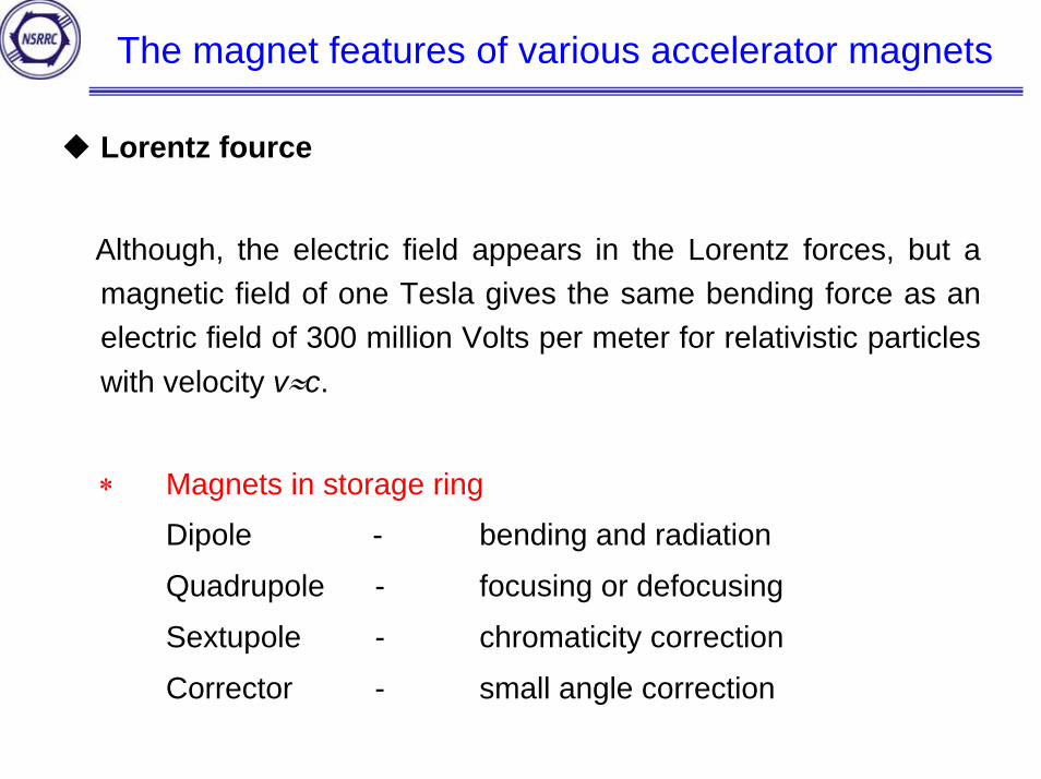
Lorentz fource

Although, the electric field appears in the Lorentz forces, but a magnetic field of one Tesla gives the same bending force as an electric field of 300 million Volts per meter for relativistic particles with velocity v≈c.

∗ Magnets in storage ringDipole - bending and radiation

Quadrupole - focusing or defocusing

Sextupole - chromaticity correction

Corrector - small angle correction

The magnet features of various accelerator magnet

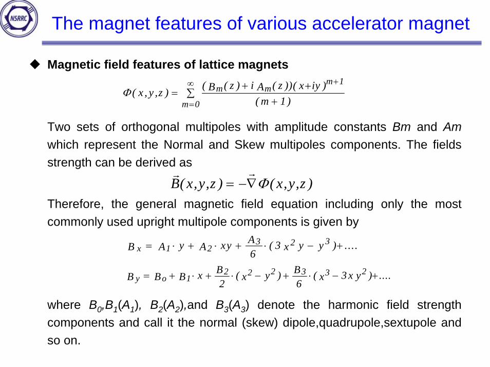
Magnetic field features of lattice magnets

Two sets of orthogonal multipoles with amplitude constants Bm and Amwhich represent the Normal and Skew multipoles components. The fields strength can be derived as

Therefore, the general magnetic field equation including only the most commonly used upright multipole components is given by

where B0,B1(A1), B2(A2),and B3(A3) denote the harmonic field strength components and call it the normal (skew) dipole,quadrupole,sextupole and so on.

Φ ( , , ) ( ( ) ( ))( )( )

x y z B z i A z x iym

m mm

m=

+ ++

∑+

=

∞ 1

0 1

r rB x y z x y z( , , ) ( , , )= −∇Φ

xB A y A xy A x y y= ⋅ + ⋅ + ⋅ − +1 23 2 3

63( ) ....

y oB B B x B x y B x x y= + ⋅ + ⋅ − + ⋅ − +12 2 2 3 3 2

2 63( ) ( ) ....

Magnet for accelerator lattice system

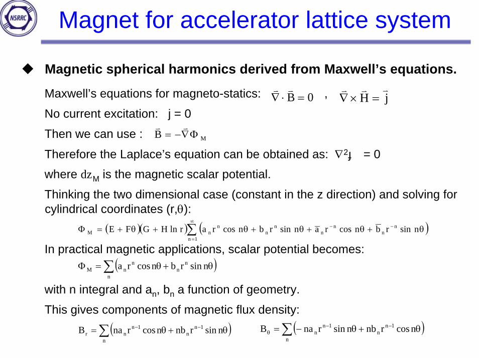
Magnetic spherical harmonics derived from Maxwell’s equations.

Maxwell’s equations for magneto-statics: ,

No current excitation: j = 0

Then we can use :

Therefore the Laplace’s equation can be obtained as: ∇2Φ = 0

where ΦM is the magnetic scalar potential.

Thinking the two dimensional case (constant in the z direction) and solving for cylindrical coordinates (r,θ):

In practical magnetic applications, scalar potential becomes:

with n integral and an, bn a function of geometry.

This gives components of magnetic flux density:

0B =⋅∇vv

jHvvv

=×∇

MB Φ∇−=vv

( )( ) ( )∑∞

=

−− θ+θ+θ+θ+θ+=Φ1n

nn

nn

nn

nnM nsinrbncosransinrbncosrarlnHGFE

( )∑ θ+θ=Φn

nn

nnM nsinrbncosra

( )∑ θ+θ= −−

n

1nn

1nnr nsinrnbncosrnaB ( )∑ θ+θ−= −−

θn

1nn

1nn ncosrnbnsinrnaB

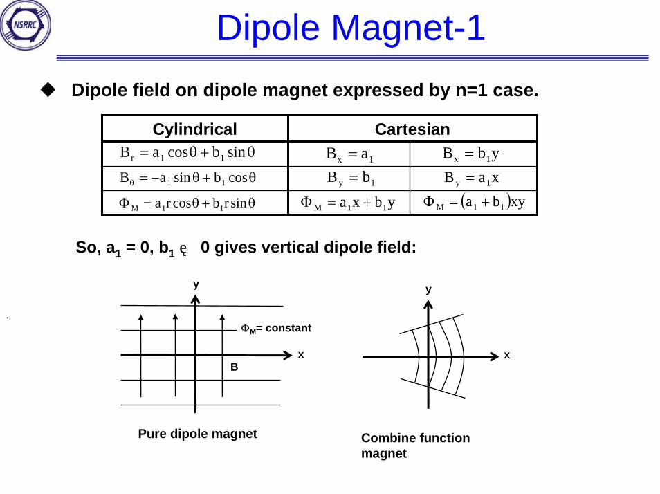
Dipole Magnet-1Dipole field on dipole magnet expressed by n=1 case.

So, a1 = 0, b1≠ 0 gives vertical dipole field:

Cylindrical Cartesian

.

θ+θ−=θ cosbsinaB 11

θ+θ= sinbcosaB 11r

θ+θ=Φ sinrbcosra 11M

1x aB = ybB 1x =

ybxa 11M +=Φ ( )xyba 11M +=Φ1y bB = xaB 1y =

B

ΦM= constant

y

x

Pure dipole magnet

y

x

Combine function magnet

Dipole Magnet-2b1 = 0, a1≠ 0 gives horizontal dipole field (which is about rotated )

By

x

By

x

12×π

Separate function dipole Combine function dipole

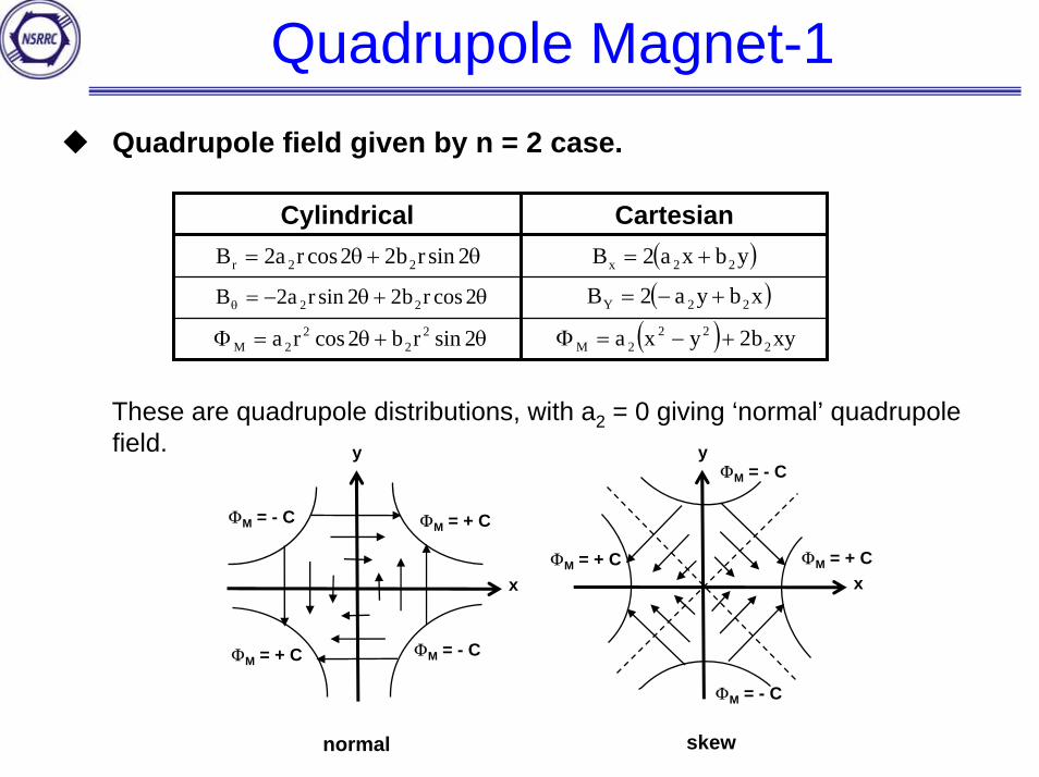
Quadrupole Magnet-1Quadrupole field given by n = 2 case.

These are quadrupole distributions, with a2 = 0 giving ‘normal’ quadrupolefield.

Cylindrical Cartesianθ+θ= 2sinrb22cosra2B 22r

θ+θ−=θ 2cosrb22sinra2B 22

θ+θ=Φ 2sinrb2cosra 22

22M

( )ybxa2B 22x +=

( )xbya2B 22Y +−=

( ) xyb2yxa 222

2M +−=Φ

y

ΦM = + CΦM = - C

ΦM = + C ΦM = - C

x

normal skew

y

ΦM = + C

ΦM = - C

ΦM = + C

ΦM = - C

x

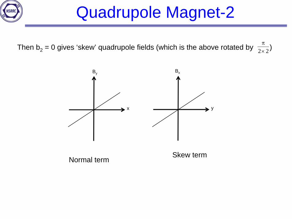
Quadrupole Magnet-2

Then b2 = 0 gives ‘skew’ quadrupole fields (which is the above rotated by )22×π

x

By

y

Bx

Skew termNormal term

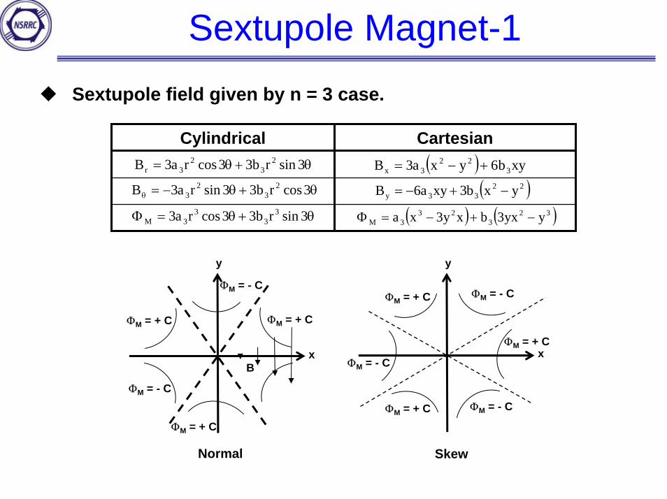
Sextupole Magnet-1Sextupole field given by n = 3 case.

Cylindrical Cartesianθ+θ= 3sinrb33cosra3B 2

32

3r

θ+θ−=θ 3cosrb33sinra3B 23

23

θ+θ=Φ 3sinrb33cosra3 33

33M

( ) xyb6yxa3B 322

3x +−=

( )2233y yxb3xya6B −+−=

( ) ( )323

233M yyx3bxy3xa −+−=Φ

ΦM = + C

ΦM = - C

ΦM = + C

ΦM = + C

ΦM = - C

B

y

x

Normal

ΦM = + C

ΦM = - C

ΦM = + C

ΦM = + C

ΦM = - C

ΦM = - C

y

x

Skew

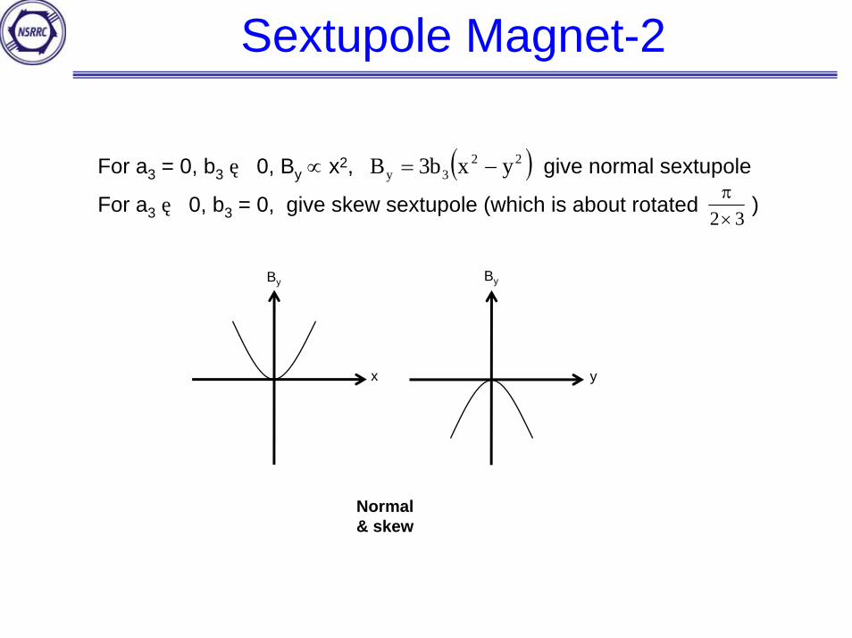
Sextupole Magnet-2

For a3 = 0, b3≠ 0, By ∝ x2, give normal sextupole

For a3≠ 0, b3 = 0, give skew sextupole (which is about rotated )

( )223y yxb3B −=

32×π

By

x

By

y

Normal & skew

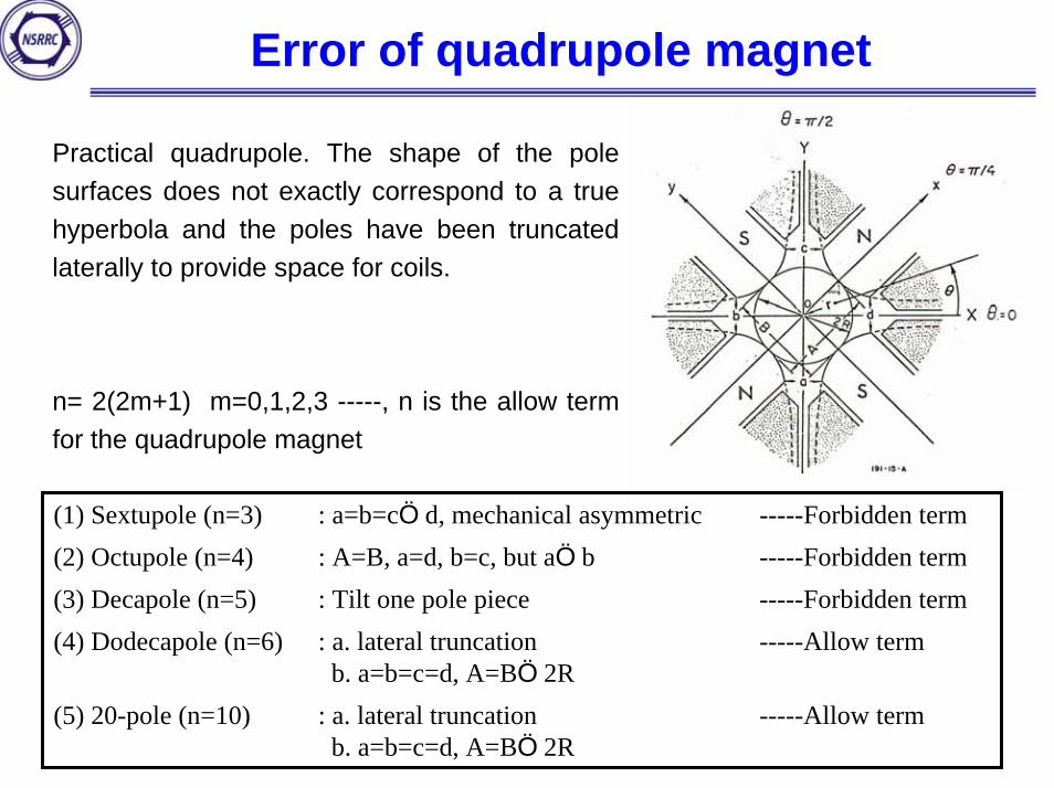
Error of quadrupole magnet

Practical quadrupole. The shape of the pole surfaces does not exactly correspond to a true hyperbola and the poles have been truncated laterally to provide space for coils.

n= 2(2m+1) m=0,1,2,3 -----, n is the allow term for the quadrupole magnet

(1) Sextupole (n=3) : a=b=c≠d, mechanical asymmetric -----Forbidden term(2) Octupole (n=4) : A=B, a=d, b=c, but a≠b -----Forbidden term(3) Decapole (n=5) : Tilt one pole piece -----Forbidden term(4) Dodecapole (n=6) : a. lateral truncation

b. a=b=c=d, A=B≠2R-----Allow term

(5) 20-pole (n=10) : a. lateral truncationb. a=b=c=d, A=B≠2R

-----Allow term

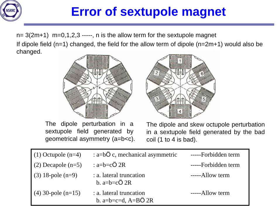
Error of sextupole magnetn= 3(2m+1) m=0,1,2,3 -----, n is the allow term for the sextupole magnetIf dipole field (n=1) changed, the field for the allow term of dipole (n=2m+1) would also be changed.

The dipole perturbation in a sextupole field generated by geometrical asymmetry (a=b<c).

The dipole and skew octupole perturbation in a sextupole field generated by the bad coil (1 to 4 is bad).

(1) Octupole (n=4) : a=b≠c, mechanical asymmetric -----Forbidden term

(2) Decapole (n=5) : a=b=c≠2R -----Forbidden term

(3) 18-pole (n=9) : a. lateral truncationb. a=b=c≠2R

-----Allow term

(4) 30-pole (n=15) : a. lateral truncationb. a=b=c=d, A=B≠2R

-----Allow term

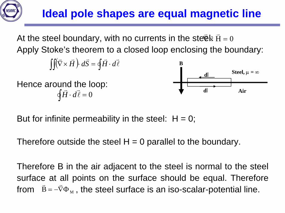
Ideal pole shapes are equal magnetic line

At the steel boundary, with no currents in the steel:Apply Stoke’s theorem to a closed loop enclosing the boundary:

Hence around the loop:

But for infinite permeability in the steel: H = 0;

Therefore outside the steel H = 0 parallel to the boundary.

Therefore B in the air adjacent to the steel is normal to the steel surface at all points on the surface should be equal. Therefore from , the steel surface is an iso-scalar-potential line.

0H =×∇vv

( )∫∫ ∫ ⋅=⋅×∇ lvvvvv

dHSdH B

dl

dl

Steel, µ = ∞

Air∫ =⋅ 0lvv

dH

MB Φ∇−=vv

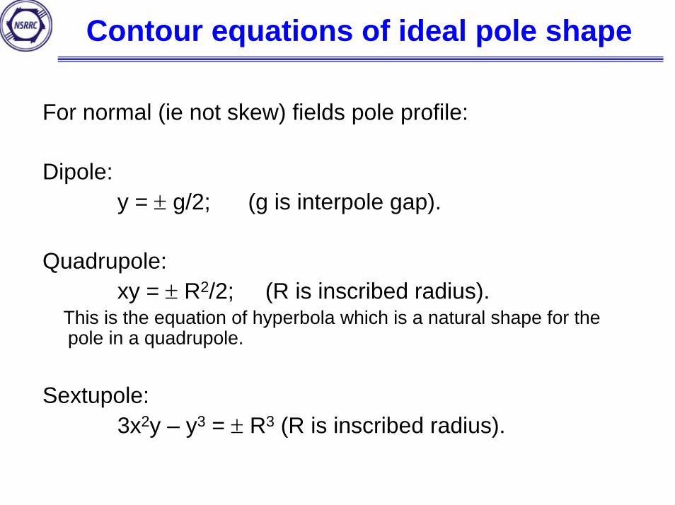
Contour equations of ideal pole shape

For normal (ie not skew) fields pole profile:

Dipole:y = ± g/2; (g is interpole gap).

Quadrupole:xy = ± R2/2; (R is inscribed radius).

This is the equation of hyperbola which is a natural shape for the pole in a quadrupole.

Sextupole:3x2y – y3 = ± R3 (R is inscribed radius).

Symmetry constraints in normal dipole, quadurpoleand sextupole geometries

Magnet Symmetry Constraintφ(θ) = -φ(2π-θ) All an = 0;φ(θ) = φ(π-θ) bn non-zero only for:

n=(2j-1)=1,3,5,etc; (2n)φ(θ) = -φ(π-θ) bn = 0 for all odd n;φ(θ) = -φ(2π-θ) All an = 0;φ(θ) = φ(π/2-θ) bn non-zero only for:

n=2(2j-1)=2,6,10,etc; (2n)φ(θ) = -φ(2π/3-θ)φ(θ) = -φ(4π/3-θ)

bn = 0 for all n not multiples of 3;

φ(θ) = -φ(2π-θ) All an = 0;φ(θ) = φ(π/3-θ) bn non-zero only for:

n=3(2j-1)=3,9,15,etc. (2n)

Sextupole

Quadrupole

Dipole

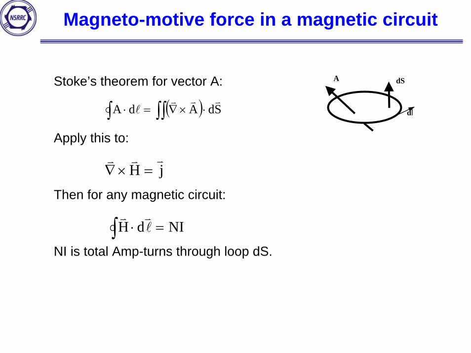
Magneto-motive force in a magnetic circuit

Stoke’s theorem for vector A:

Apply this to:

Then for any magnetic circuit:

NI is total Amp-turns through loop dS.

dl

dSA

( )∫ ∫∫ ⋅×∇=⋅ SdAdAvvv

l

jHvvv

=×∇

∫ =⋅ NIdH lvv

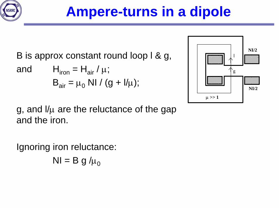
Ampere-turns in a dipole

µ >> 1

g

lNI/2

NI/2

B is approx constant round loop l & g,and Hiron = Hair / µ;

Bair = µ0 NI / (g + l/µ);

g, and l/µ are the reluctance of the gap and the iron.

Ignoring iron reluctance:NI = B g /µ0

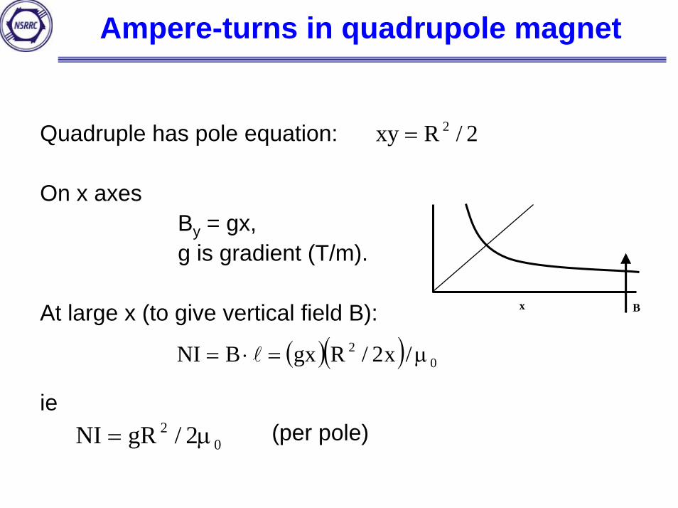
Ampere-turns in quadrupole magnet

Quadruple has pole equation:

On x axesBy = gx,g is gradient (T/m).

At large x (to give vertical field B):

ie(per pole)

2/Rxy 2=

( )( ) 02 /x2/RgxBNI µ=⋅= l

02 2/gRNI µ=

Bx

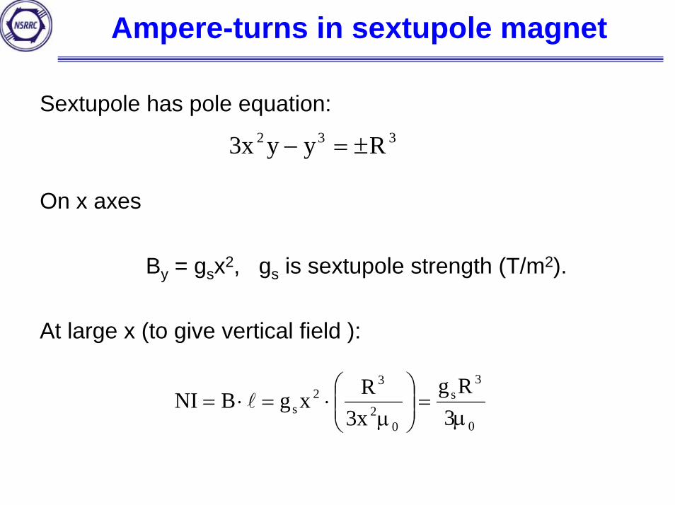
Ampere-turns in sextupole magnet

Sextupole has pole equation:

On x axes

By = gsx2, gs is sextupole strength (T/m2).

At large x (to give vertical field ):

332 Ryyx3 ±=−

0

3s

02

32

s 3Rg

x3RxgBNI

µ=⎟⎟

⎠

⎞⎜⎜⎝

⎛µ

⋅=⋅= l

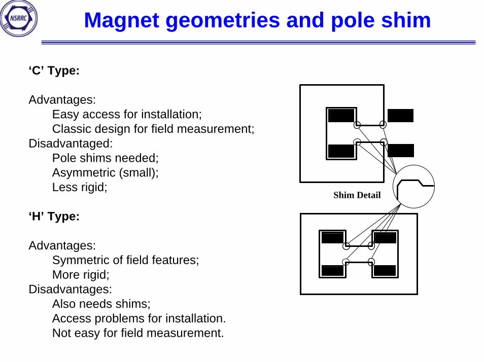
Magnet geometries and pole shim

‘C’ Type:

Advantages:Easy access for installation;Classic design for field measurement;

Disadvantaged:Pole shims needed;Asymmetric (small);Less rigid;

‘H’ Type:

Advantages:Symmetric of field features;More rigid;

Disadvantages:Also needs shims;Access problems for installation.Not easy for field measurement.

Shim Detail

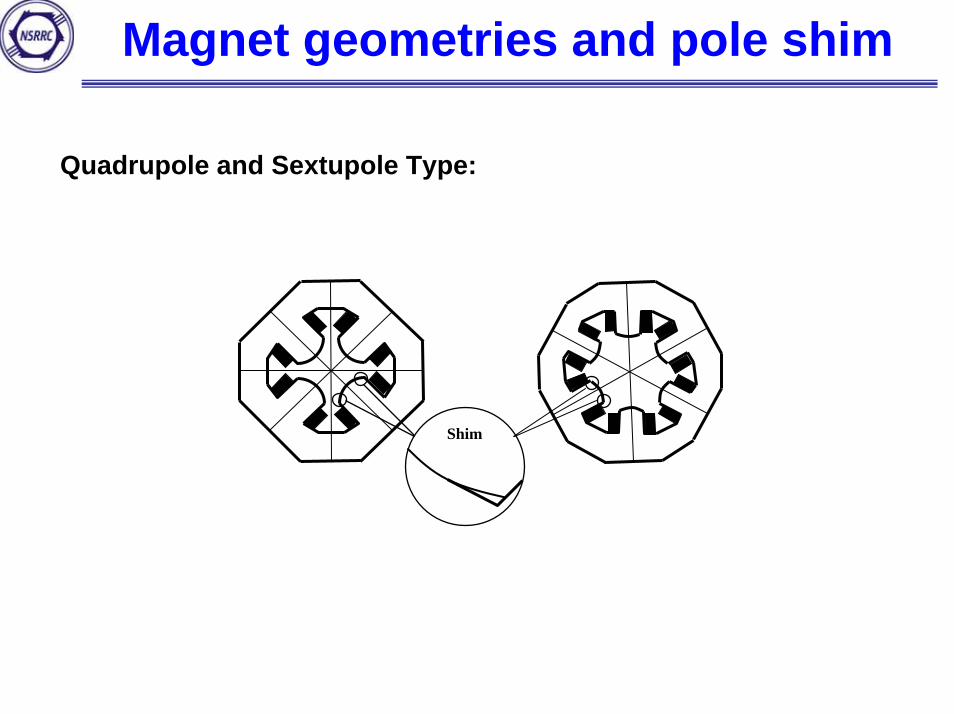
Magnet geometries and pole shim

Quadrupole and Sextupole Type:

Shim

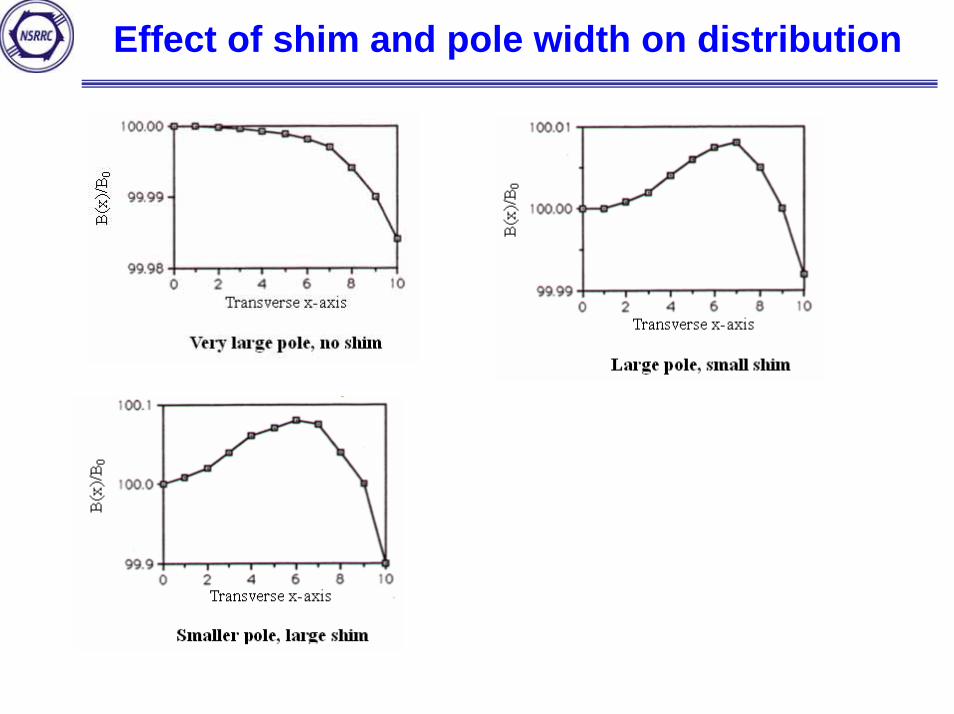
Effect of shim and pole width on distribution

Magnet chamfer for avoiding field saturation at magnet edge

Chamfering at both sides of dipole magnet to compensate for the sextupole components and the allow harmonic terms.

Chamfering at both sides of the magnet edge to compensate for the 12-pole (18-pole) on quadrupole(sextupole) magnets and their allow harmonic terms.

Chamfering means to cut the end pole along 45° on the longitudinal axis (z-axis) to avoid the field saturation at magnet edge.

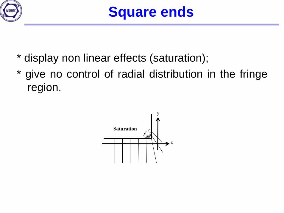
Square ends

* display non linear effects (saturation);* give no control of radial distribution in the fringe

region.

Saturation

y

z

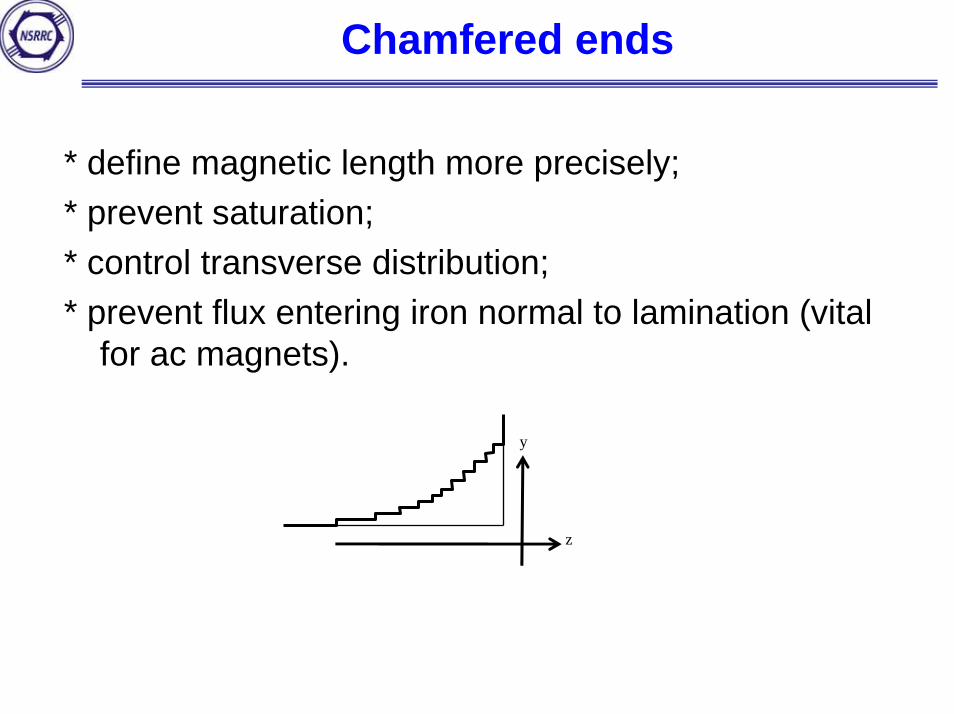
Chamfered ends

* define magnetic length more precisely;* prevent saturation;* control transverse distribution;* prevent flux entering iron normal to lamination (vital

for ac magnets).

y

z

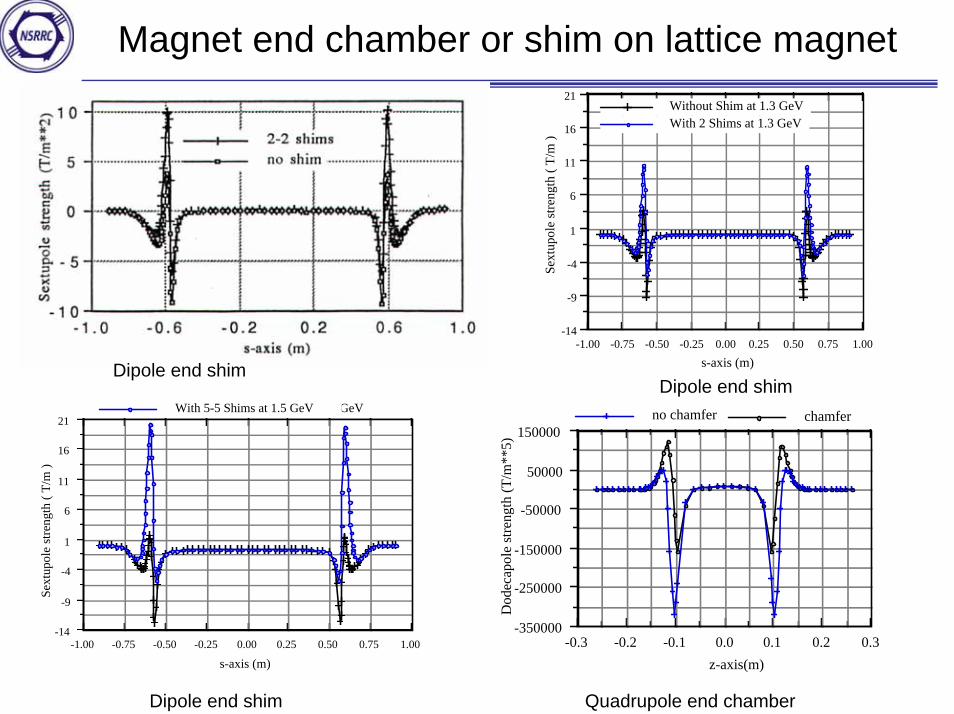
Magnet end chamber or shim on lattice magnet

1.000.750.500.250.00-0.25-0.50-0.75-1.00-14

-9

-4

1

6

11

16

21Without Shim at 1.5 GeVWith 5-5 Shims at 1.5 GeV

s-axis (m)

Sext

upol

e st

reng

th (

T/m

)

1.000.750.500.250.00-0.25-0.50-0.75-1.00-14

-9

-4

1

6

11

16

21Without Shim at 1.3 GeVWith 2 Shims at 1.3 GeV

s-axis (m)

Sext

upol

e st

reng

th (

T/m

)

0.30.20.10.0-0.1-0.2-0.3-350000

-250000

-150000

-50000

50000

150000chamferno chamfer

z-axis(m)

Dod

ecap

ole

stre

ngth

(T/m

**5)

Dipole end shimDipole end shim

Dipole end shim Quadrupole end chamber

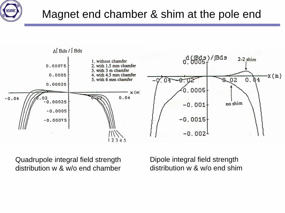
Magnet end chamber & shim at the pole end

Dipole integral field strength distribution w & w/o end shim

Quadrupole integral field strength distribution w & w/o end chamber

The trade-off of current density in coils

j = NI/Swhere:

j is the current density,S the cross section area of copper in the coil;NI is the required Amp-turns.

EC = G (NI)2/Stherefore:

EC = (G NI) jHere:

EC is energy loss in coil conductor,G is a geometrical constant factor and as function of µ.

Then, for constant NI and energy will depend on current j.

Magnet capital costs (coil & yoke materials and construction, assembly, power supply testing and transport) vary as the size of the magnet ieas 1/j.

Variation of magnet parameters with N and j (fixed NI)

I ∝ 1/N, Rmagnet ∝ N2 j, Vmagnet ∝ N j, Power ∝ j

R (Ω)=ρCu(L(m)/A(m2)=1.7x10-8 (L/A) where L and A are the

total length and cross section l area of the coil, respectively.

Ampere-turn determination

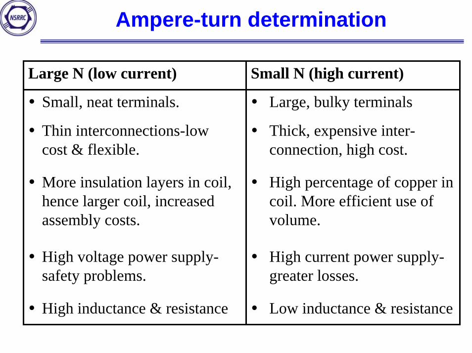
Large N (low current) Small N (high current)

Small, neat terminals. Large, bulky terminals

Thin interconnections-low cost & flexible.

Thick, expensive inter-connection, high cost.

More insulation layers in coil, hence larger coil, increased assembly costs.

High percentage of copper in coil. More efficient use of volume.

High voltage power supply-safety problems.

High current power supply-greater losses.

High inductance & resistance Low inductance & resistance

Flux at magnet gap

g

b

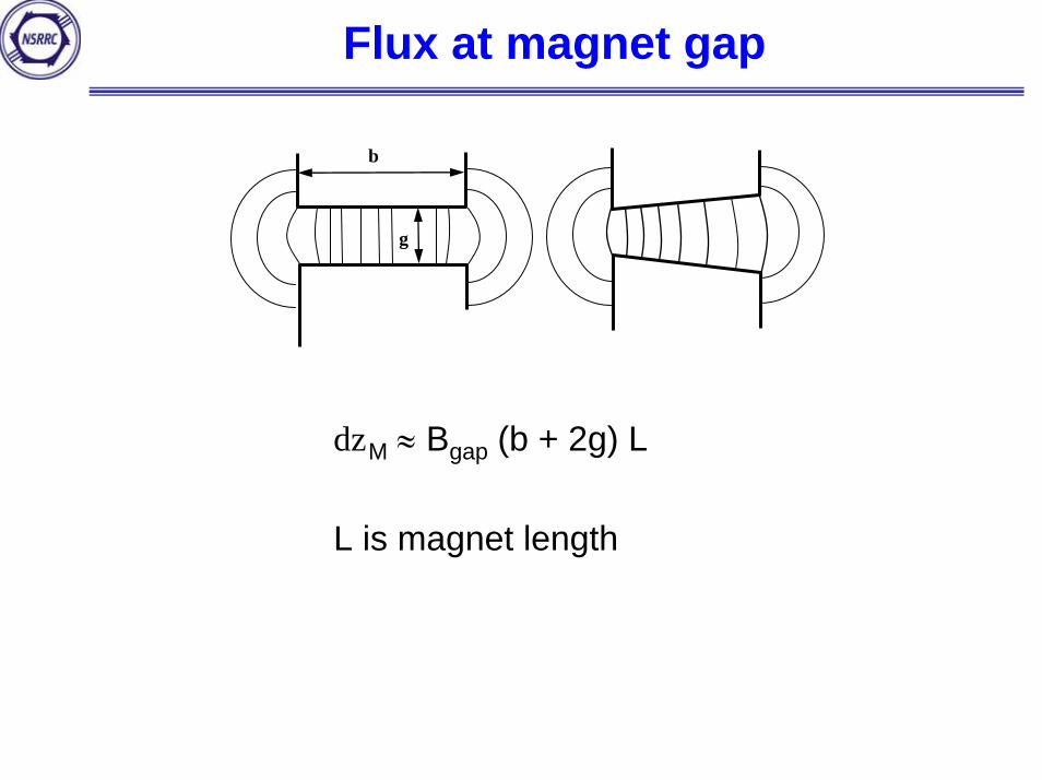
ΦM ≈ Bgap (b + 2g) L

L is magnet length

Residual field in gapped magnets

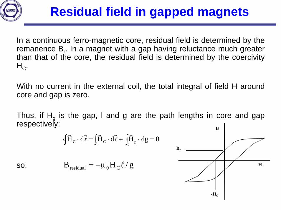
In a continuous ferro-magnetic core, residual field is determined by the remanence Br. In a magnet with a gap having reluctance much greater than that of the core, the residual field is determined by the coercivityHC.

With no current in the external coil, the total integral of field H around core and gap is zero.

Thus, if Hg is the gap, l and g are the path lengths in core and gap respectively:

so,

∫ ∫∫ =⋅+⋅=⋅l

vvlvv

lvv

g gCC 0gdHdHdH

g/HB C0residual lµ−=

-HC

Br

B

H

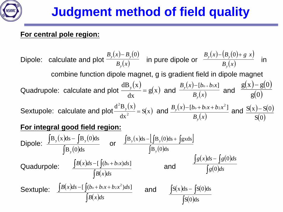
Judgment method of field qualityFor central pole region:

Dipole: calculate and plot in pure dipole or in

combine function dipole magnet, g is gradient field in dipole magnet

Quadrupole: calculate and plot and and

Sextupole: calculate and plot and and

For integral good field region:

Dipole: or

Quadurpole: and

Sextuple: and

( ) ( )( )xBBxB

y

yy 0− ( ) ( )( )( )xB

xgBxB

y

yy +− 0

( ) ( )xgdx

xdBy =( ) ( )

( )0g0gxg −

( ) ( )xSdx

xBd2

y2

= ( ) ( )( )0S

0SxS −

( ) ( )( )∫

∫ ∫−ds0B

ds0BdsxB

y

yy ( ) ( )[ ]( )∫

∫ ∫∫ +−

ds0B

gxdsds0BdsxB

y

yy

( )( )∫

∫ ∫ +−

dsxB

dsxbbdsxB o ])([ 1

( )( )xB

xbbxB

y

oy ][ 1+−

( )( )xB

xbxbbxB

y

oy ][ 221 ++−

( ) ( )( )∫

∫ ∫−dsg

dsgdsxg

0

0

( ) ( )( )∫

∫ ∫−ds0S

ds0SdsxS( )( )∫

∫ ∫ ++−

dsxB

dsxbxbbdsxB o ])([ 221

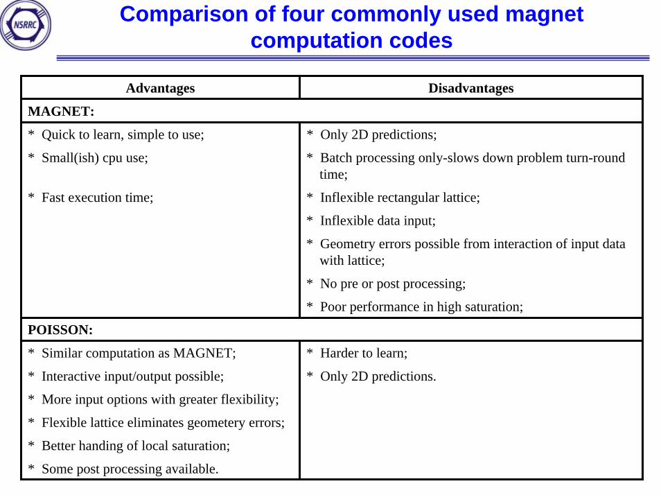
Comparison of four commonly used magnet computation codes

Advantages Disadvantages

MAGNET:

* Quick to learn, simple to use; * Only 2D predictions;

* Small(ish) cpu use; * Batch processing only-slows down problem turn-round time;

* Fast execution time; * Inflexible rectangular lattice;

* Inflexible data input;

* Geometry errors possible from interaction of input data with lattice;

* No pre or post processing;

* Poor performance in high saturation;

POISSON:

* Similar computation as MAGNET; * Harder to learn;

* Interactive input/output possible; * Only 2D predictions.

* More input options with greater flexibility;

* Flexible lattice eliminates geometery errors;

* Better handing of local saturation;

* Some post processing available.

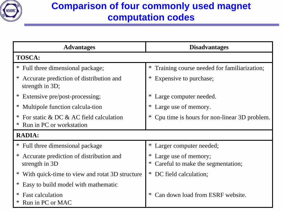
Comparison of four commonly used magnet computation codes

Advantages Disadvantages

TOSCA:

* Full three dimensional package; * Training course needed for familiarization;

* Accurate prediction of distribution and strength in 3D;

* Expensive to purchase;

* Extensive pre/post-processing; * Large computer needed.

* Multipole function calcula-tion * Large use of memory.

* For static & DC & AC field calculation* Run in PC or workstation

* Cpu time is hours for non-linear 3D problem.

RADIA:

* Full three dimensional package * Larger computer needed;

* Accurate prediction of distribution and strength in 3D

* Large use of memory;* Careful to make the segmentation;

* With quick-time to view and rotat 3D structure * DC field calculation;

* Easy to build model with mathematic

* Fast calculation * Run in PC or MAC

* Can down load from ESRF website.

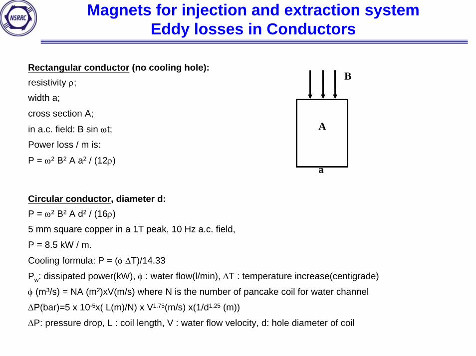
Magnets for injection and extraction systemEddy losses in Conductors

Rectangular conductor (no cooling hole):resistivity ρ;width a;

cross section A;

in a.c. field: B sin ωt;Power loss / m is:

P = ω2 B2 A a2 / (12ρ)

Circular conductor, diameter d:P = ω2 B2 A d2 / (16ρ)5 mm square copper in a 1T peak, 10 Hz a.c. field,

P = 8.5 kW / m.

Cooling formula: P = (φ ∆T)/14.33

Pw: dissipated power(kW), φ : water flow(l/min), ∆T : temperature increase(centigrade)

φ (m3/s) = NA (m2)xV(m/s) where N is the number of pancake coil for water channel

∆P(bar)=5 x 10-5x( L(m)/N) x V1.75(m/s) x(1/d1.25 (m))

∆P: pressure drop, L : coil length, V : water flow velocity, d: hole diameter of coil

A

B

a

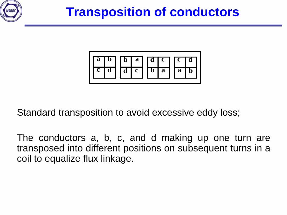
Transposition of conductors

a bc d

abcd ab

cda bc d

Standard transposition to avoid excessive eddy loss;

The conductors a, b, c, and d making up one turn are transposed into different positions on subsequent turns in a coil to equalize flux linkage.

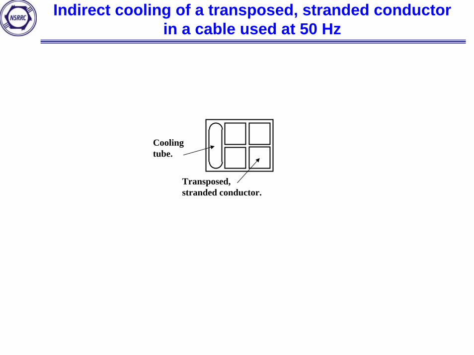
Indirect cooling of a transposed, stranded conductor in a cable used at 50 Hz

Cooling tube.

Transposed, stranded conductor.

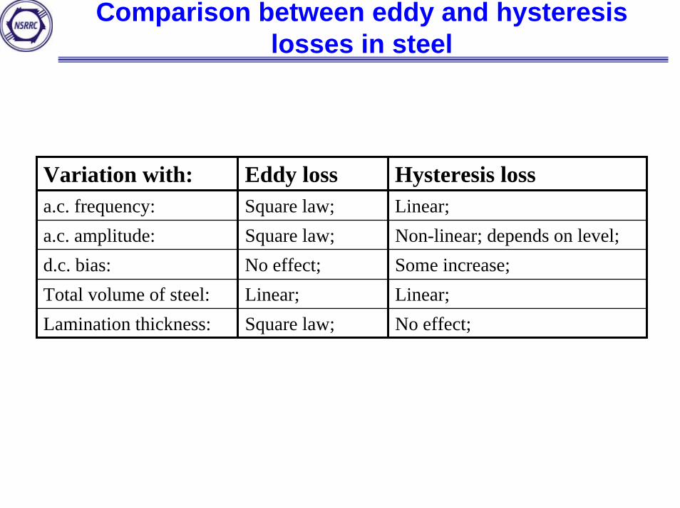
Comparison between eddy and hysteresislosses in steel

Variation with: Eddy loss Hysteresis lossa.c. frequency: Square law; Linear;a.c. amplitude: Square law; Non-linear; depends on level;d.c. bias: No effect; Some increase;Total volume of steel: Linear; Linear;Lamination thickness: Square law; No effect;

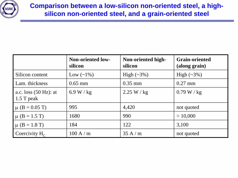
Comparison between a low-silicon non-oriented steel, a high-silicon non-oriented steel, and a grain-oriented steel

Non-oriented low-silicon

Non-oriented high-silicon

Grain-oriented (along grain)

Silicon content Low (~1%) High (~3%) High (~3%)

Lam. thickness 0.65 mm 0.35 mm 0.27 mm

a.c. loss (50 Hz): at 1.5 T peak

6.9 W / kg 2.25 W / kg 0.79 W / kg

µ (B = 0.05 T) 995 4,420 not quoted

µ (B = 1.5 T) 1680 990 > 10,000

µ (B = 1.8 T) 184 122 3,100

Coercivity HC 100 A / m 35 A / m not quoted

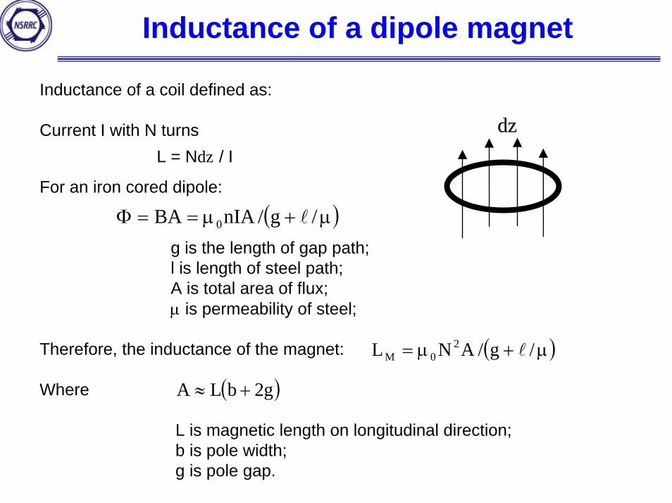
Inductance of a dipole magnet

Inductance of a coil defined as:

Current I with N turnsL = NΦ / I

For an iron cored dipole:

g is the length of gap path;l is length of steel path;A is total area of flux;µ is permeability of steel;

Therefore, the inductance of the magnet:

Where

L is magnetic length on longitudinal direction;b is pole width;g is pole gap.

Φ

( )µ+µ==Φ /g/nIABA 0 l

( )µ+µ= /g/ANL 20M l

( )g2bLA +≈

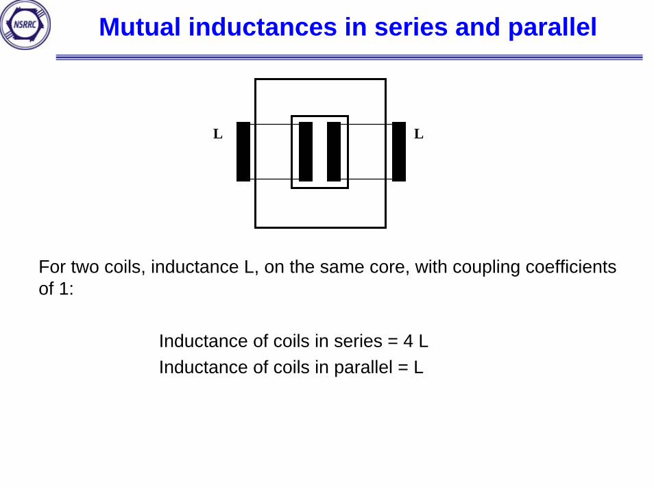
Mutual inductances in series and parallel

L L

For two coils, inductance L, on the same core, with coupling coefficients of 1:

Inductance of coils in series = 4 LInductance of coils in parallel = L

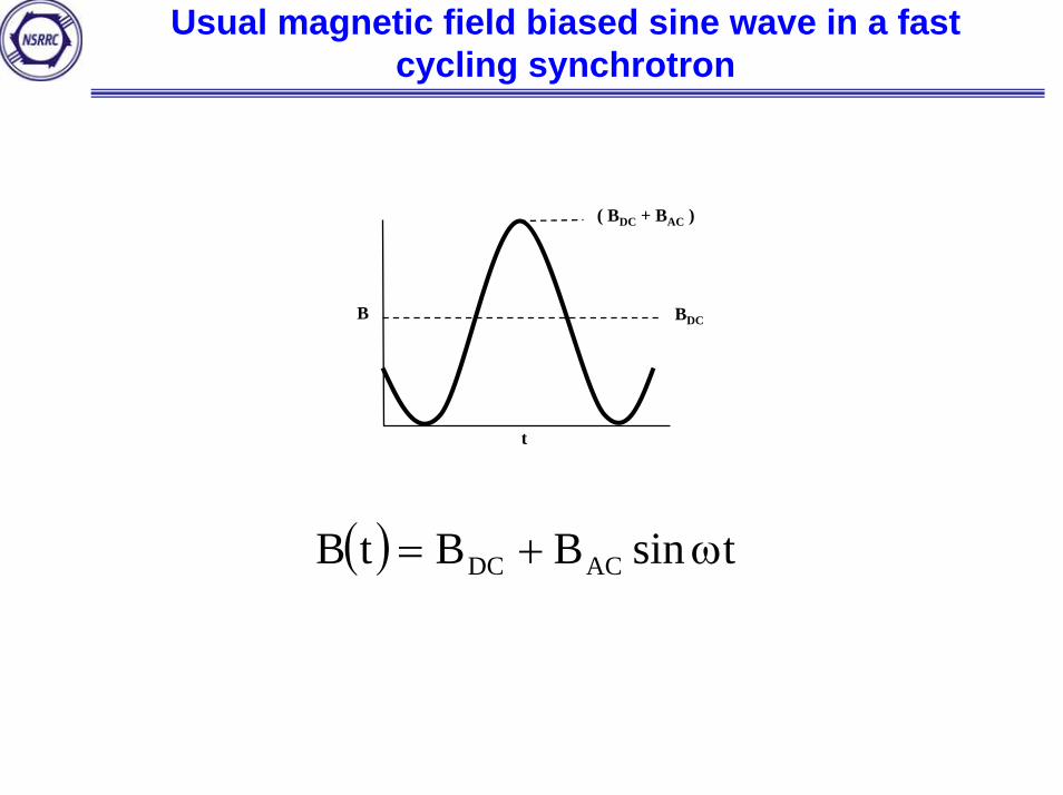
Usual magnetic field biased sine wave in a fast cycling synchrotron

t

B BDC

( BDC + BAC )

( ) tsinBBtB ACDC ω+=

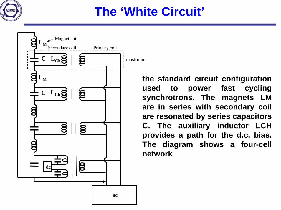
The ‘White Circuit’

LM

LM

C LCh

C LCh

dc

ac

Secondary coil Primary coil

Magnet coil

transformer

the standard circuit configuration used to power fast cycling synchrotrons. The magnets LM are in series with secondary coil are resonated by series capacitors C. The auxiliary inductor LCH provides a path for the d.c. bias. The diagram shows a four-cell network

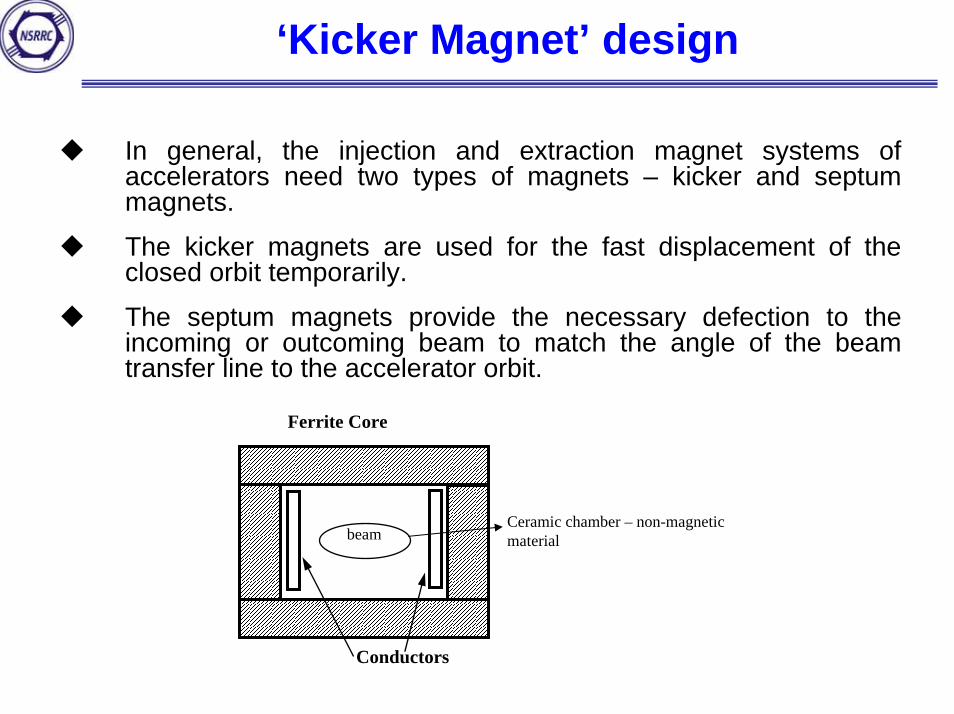
‘Kicker Magnet’ design

In general, the injection and extraction magnet systems of accelerators need two types of magnets – kicker and septum magnets.

The kicker magnets are used for the fast displacement of the closed orbit temporarily.

The septum magnets provide the necessary defection to the incoming or outcoming beam to match the angle of the beam transfer line to the accelerator orbit.

beam

Conductors

Ferrite Core

Ceramic chamber – non-magnetic material

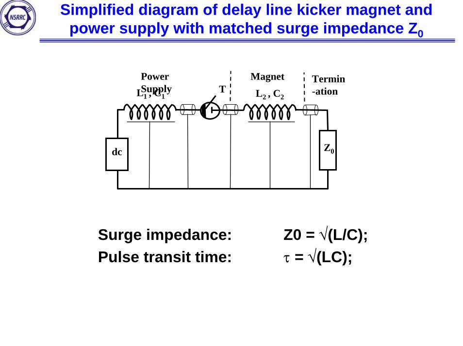
Simplified diagram of delay line kicker magnet and power supply with matched surge impedance Z0

dc Z0

Power Supply

Magnet Termin-ationL2 , C2

TL1 , C1

Surge impedance: Z0 = √(L/C);Pulse transit time: τ = √(LC);

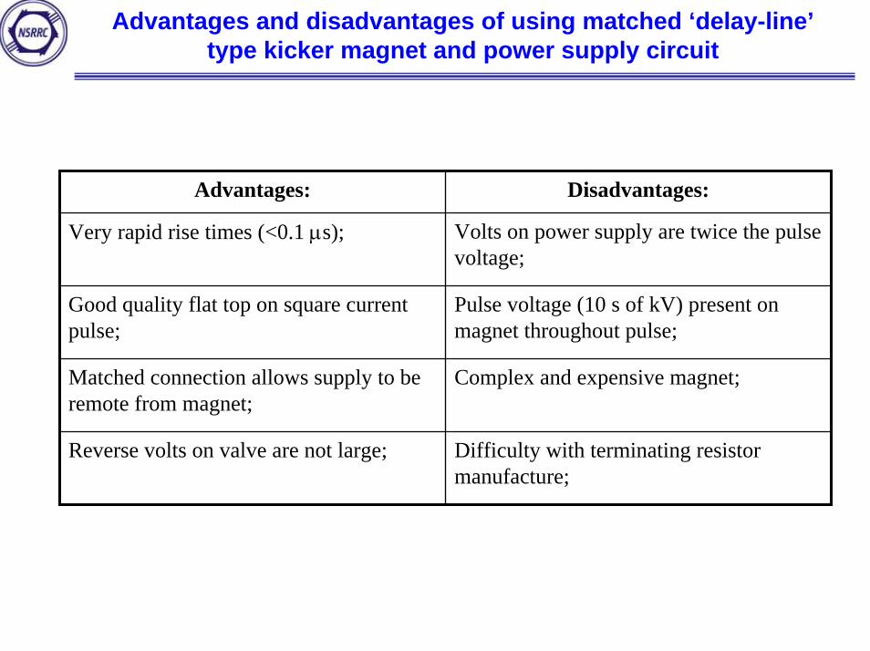
Advantages and disadvantages of using matched ‘delay-line’type kicker magnet and power supply circuit

Advantages: Disadvantages:

Very rapid rise times (<0.1 µs); Volts on power supply are twice the pulse voltage;

Good quality flat top on square current pulse;

Pulse voltage (10 s of kV) present on magnet throughout pulse;

Matched connection allows supply to be remote from magnet;

Complex and expensive magnet;

Reverse volts on valve are not large; Difficulty with terminating resistor manufacture;

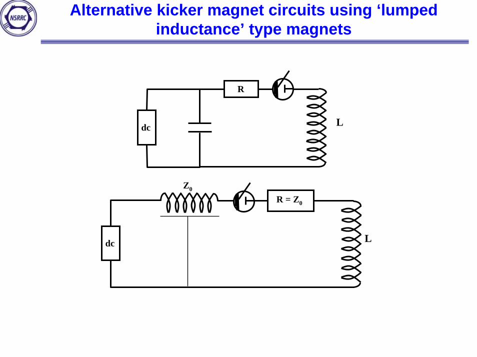
Alternative kicker magnet circuits using ‘lumped inductance’ type magnets

dc

R

L

dc

R = Z0

Z0

L

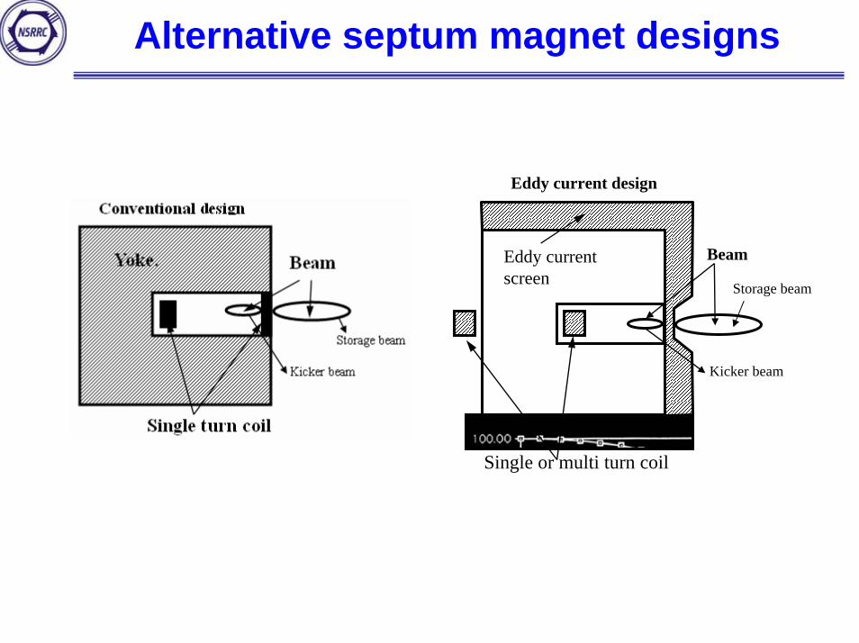
Alternative septum magnet designs

Eddy current screen

Single or multi turn coil

Eddy current design

Beam

Storage beam

Kicker beam

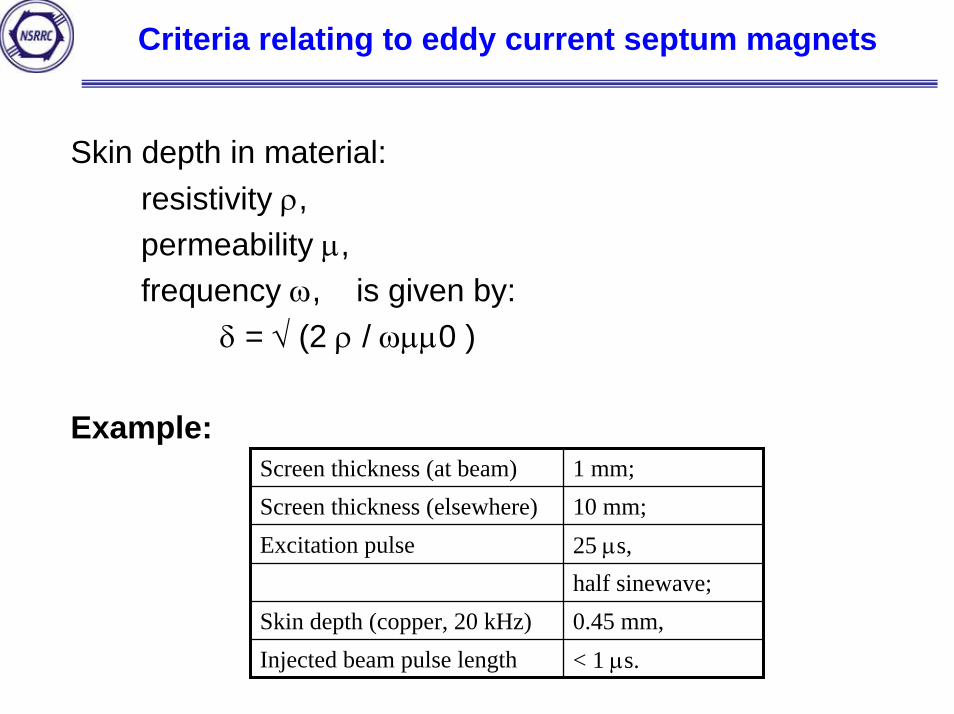
Criteria relating to eddy current septum magnets

Skin depth in material:resistivity ρ,permeability µ,frequency ω, is given by:

δ = √ (2 ρ / ωµµ0 )

Example:Screen thickness (at beam) 1 mm;Screen thickness (elsewhere) 10 mm;Excitation pulse 25 µs,

half sinewave;Skin depth (copper, 20 kHz) 0.45 mm,Injected beam pulse length < 1 µs.

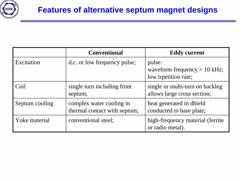
Features of alternative septum magnet designs

Conventional Eddy currentExcitation d.c. or low frequency pulse; pulse:

waveform frequency > 10 kHz; low trpetition rate;

Coil single turn including front septum;

single or multi-turn on backlegallows large cross section;

Septum cooling complex water cooling in thermal contact with septum;

heat generated in dhieldconducted to base plate;

Yoke material conventional steel; high-frequency material (ferrite or radio metal).

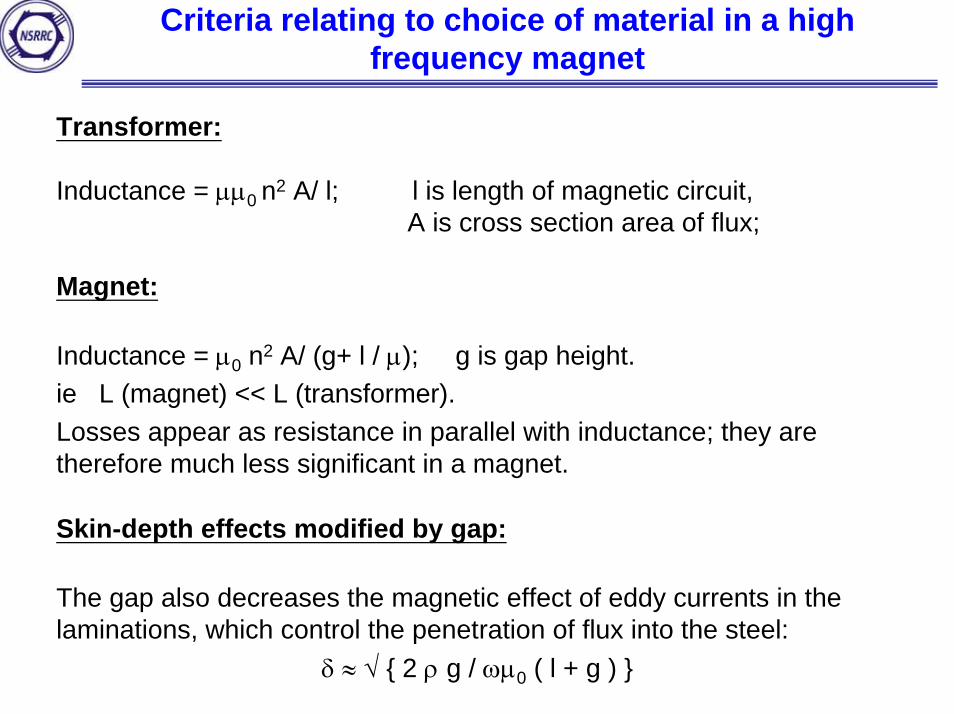
Criteria relating to choice of material in a high frequency magnet

Transformer:

Inductance = µµ0 n2 A/ l; l is length of magnetic circuit,A is cross section area of flux;

Magnet:

Inductance = µ0 n2 A/ (g+ l / µ); g is gap height.ie L (magnet) << L (transformer).Losses appear as resistance in parallel with inductance; they are therefore much less significant in a magnet.

Skin-depth effects modified by gap:

The gap also decreases the magnetic effect of eddy currents in the laminations, which control the penetration of flux into the steel:

δ ≈ √ 2 ρ g / ωµ0 ( l + g )

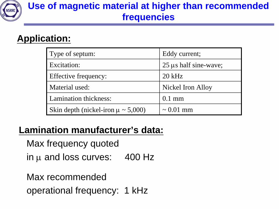
Use of magnetic material at higher than recommended frequencies

Application:Type of septum: Eddy current;Excitation: 25 µs half sine-wave;Effective frequency: 20 kHzMaterial used: Nickel Iron AlloyLamination thickness: 0.1 mmSkin depth (nickel-iron µ ~ 5,000) ~ 0.01 mm

Lamination manufacturer’s data:Max frequency quotedin µ and loss curves: 400 Hz

Max recommendedoperational frequency: 1 kHz

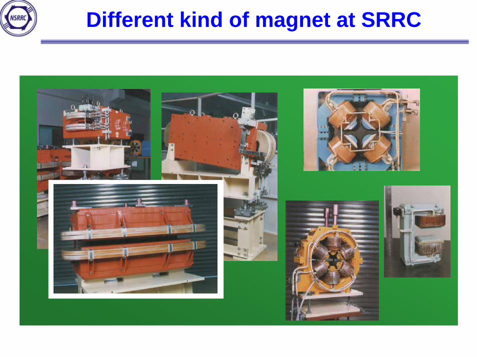
Different kind of magnet at SRRC

Reference

[1]Neil, Marks, CERN Accelerator School, fifth general accelerator physics course, Editor by S. Turner, CERN 94-01, 26 January,1994, Vol. II.[2]Handbook of accelerator physics and engineering, World Scientific publishing Co. Pte. Ltd., edited by Alexander Wu Chao and Maury Tigner(1998).[3]Jack Tanabe, Lectures of conventional magnet design, USPAS, Tucson, Arizona, January, 2000.[4]Synchrotron Radiation Sources- A Primer, World Scientific publishing Co. Pte.[5]C. H. Chang, H. H. Chen, C. S. Hwang, G. J. Hwang, and P. K. Tseng, 1994, July, "Design and Performance of the SRRC Quadrupole Magnets", IEEE Trans. on magn., 30, No. 4, (1994) 2241-2244.[6]C. H. Chang, C. S. Hwang, C. P. Hwang, G. J. Hwang, and P. K. Tseng, 1994, July, "Design, Construction and Measurement of the SRRC Sextupole Magnets", IEEE Trans. on magn., 30, No. 4, (1994) 2245-2248. (SCI)

Accelerator Magnets-2Wednesday 2 August, 2006 in YangZhou , 14:00– 17:15

Ching-Shiang Hwang (黃清鄉)

(cshwang@nsrrc.org.tw)

National Synchrotron Radiation Research Center (NSRRC), Hsinchu

Outlines

• Introduction to magnet measurement

• Classification of field measurement method and system

• Procedure of field quality control and analysis

• Example of accelerator magnet measurement

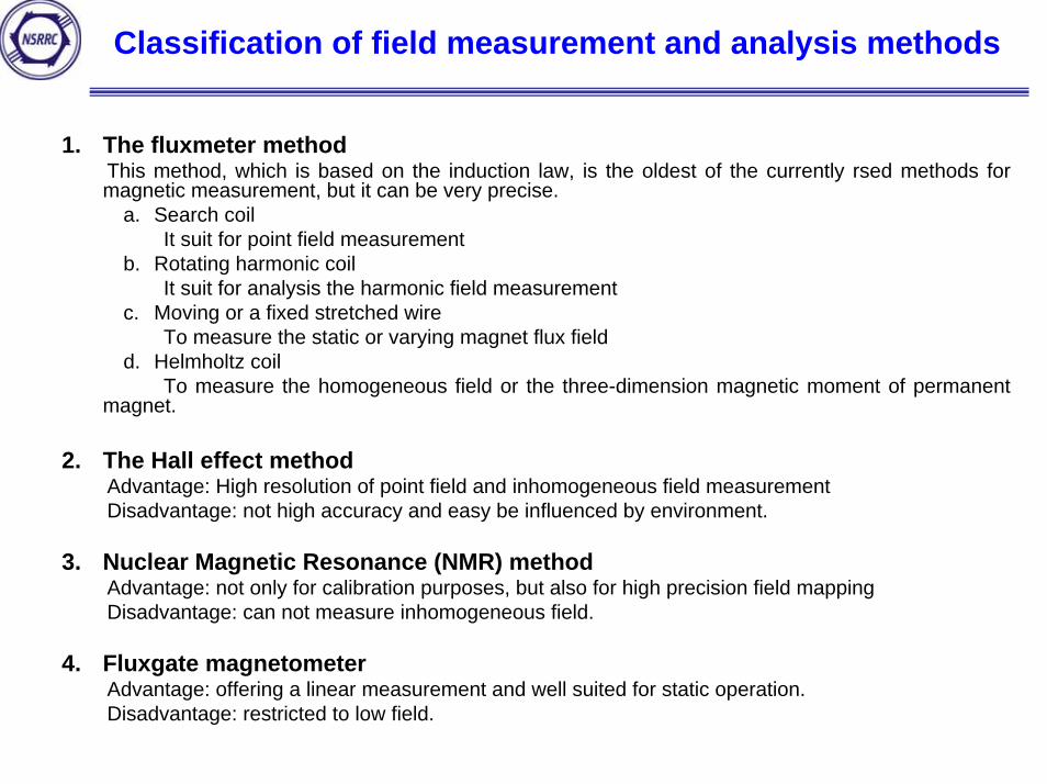
Classification of field measurement and analysis methods

1. The fluxmeter methodThis method, which is based on the induction law, is the oldest of the currently rsed methods for magnetic measurement, but it can be very precise.

a. Search coilIt suit for point field measurement

b. Rotating harmonic coilIt suit for analysis the harmonic field measurement

c. Moving or a fixed stretched wireTo measure the static or varying magnet flux field

d. Helmholtz coilTo measure the homogeneous field or the three-dimension magnetic moment of permanent

magnet.

2. The Hall effect methodAdvantage: High resolution of point field and inhomogeneous field measurementDisadvantage: not high accuracy and easy be influenced by environment.

3. Nuclear Magnetic Resonance (NMR) methodAdvantage: not only for calibration purposes, but also for high precision field mappingDisadvantage: can not measure inhomogeneous field.

4. Fluxgate magnetometerAdvantage: offering a linear measurement and well suited for static operation.Disadvantage: restricted to low field.

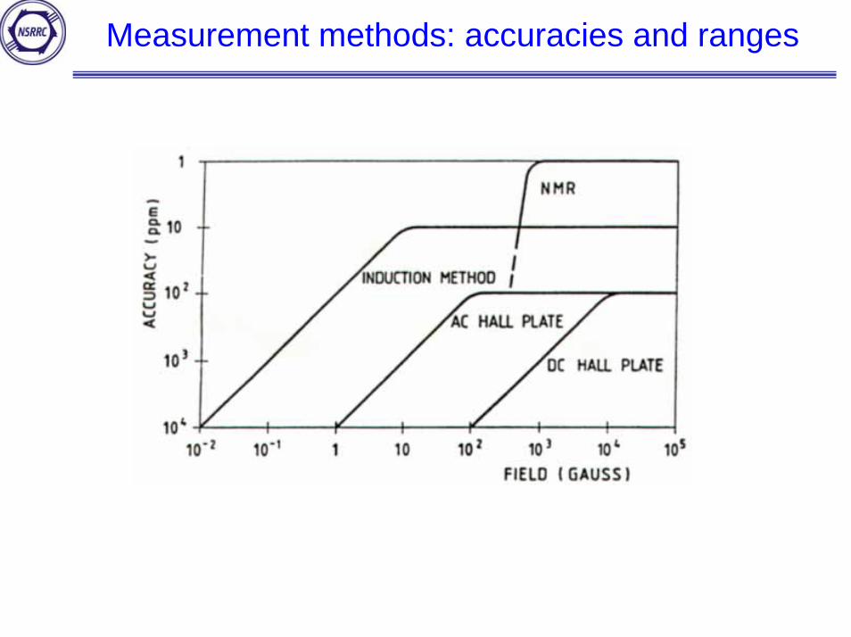
Measurement methods: accuracies and ranges

Data analysis on the Hall probe system

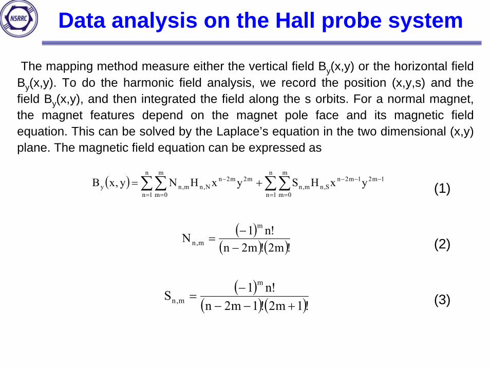
The mapping method measure either the vertical field By(x,y) or the horizontal field By(x,y). To do the harmonic field analysis, we record the position (x,y,s) and the field By(x,y), and then integrated the field along the s orbits. For a normal magnet, the magnet features depend on the magnet pole face and its magnetic field equation. This can be solved by the Laplace’s equation in the two dimensional (x,y) plane. The magnetic field equation can be expressed as

(1)

(2)

(3)

( ) ∑∑ ∑∑= = = =

−−−− +=n

1n

m

0m

n

1n

m

0m

1m21m2nS,nm,n

m2m2nN,nm,ny yxHSyxHNy,xB

( )( ) ( )!m2!m2n

!n1Nm

m,n −−

=

( )( ) ( )!1m2!1m2n

!n1Sm

m,n +−−−

=

Data analysis on the Hall probe system

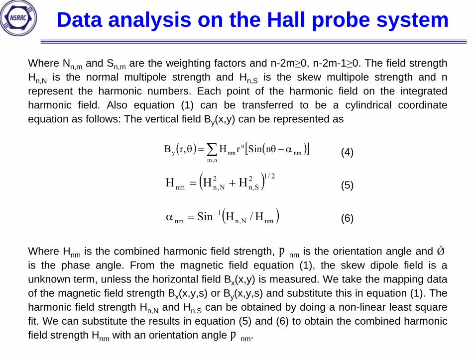
Where Nn,m and Sn,m are the weighting factors and n-2m≥0, n-2m-1≥0. The field strength Hn,N is the normal multipole strength and Hn,S is the skew multipole strength and n represent the harmonic numbers. Each point of the harmonic field on the integrated harmonic field. Also equation (1) can be transferred to be a cylindrical coordinate equation as follows: The vertical field By(x,y) can be represented as

(4)

(5)

(6)

Where Hnm is the combined harmonic field strength, αnm is the orientation angle and θis the phase angle. From the magnetic field equation (1), the skew dipole field is a unknown term, unless the horizontal field Bx(x,y) is measured. We take the mapping data of the magnetic field strength Bx(x,y,s) or By(x,y,s) and substitute this in equation (1). The harmonic field strength Hn,N and Hn,S can be obtained by doing a non-linear least square fit. We can substitute the results in equation (5) and (6) to obtain the combined harmonic field strength Hnm with an orientation angle αnm.

( ) ( )[ ]∑ α−θ=θn,m

nmn

nmy nSinrH,rB

( ) 2/12S,n

2N,nnm HHH +=

( )nmN,n1

nm H/HSin −=α

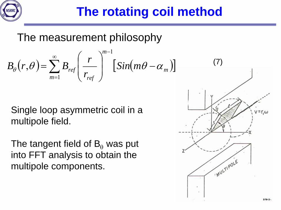
The rotating coil method

The measurement philosophy

(7)( ) ( )[ ]∑∞

=

−

−⎟⎟⎠

⎞⎜⎜⎝

⎛=

1

1

,m

m

m

refref mSin

rrBrB αθθθ

Single loop asymmetric coil in a multipole field.

The tangent field of Bθ was put into FFT analysis to obtain the multipole components.

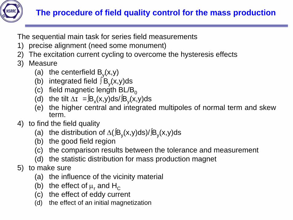
The procedure of field quality control for the mass production

The sequential main task for series field measurements1) precise alignment (need some monument)2) The excitation current cycling to overcome the hysteresis effects3) Measure

(a) the centerfield By(x,y)(b) integrated field ∫ By(x,y)ds(c) field magnetic length BL/B0(d) the tilt ∆θ=∫Bx(x,y)ds/∫By(x,y)ds(e) the higher central and integrated multipoles of normal term and skew

term.4) to find the field quality

(a) the distribution of ∆(∫By(x,y)ds)/∫By(x,y)ds(b) the good field region(c) the comparison results between the tolerance and measurement(d) the statistic distribution for mass production magnet

5) to make sure (a) the influence of the vicinity material(b) the effect of µr and HC(c) the effect of eddy current(d) the effect of an initial magnetization

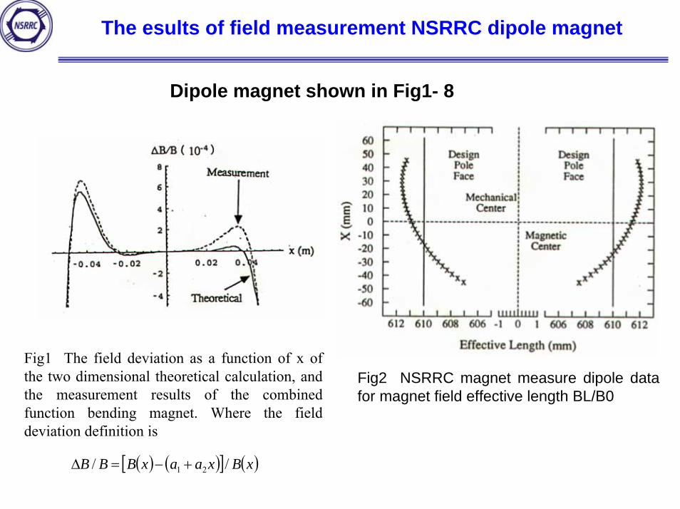
The esults of field measurement NSRRC dipole magnet

Dipole magnet shown in Fig1- 8

Fig1 The field deviation as a function of x of the two dimensional theoretical calculation, and the measurement results of the combined function bending magnet. Where the field deviation definition is

Fig2 NSRRC magnet measure dipole datafor magnet field effective length BL/B0

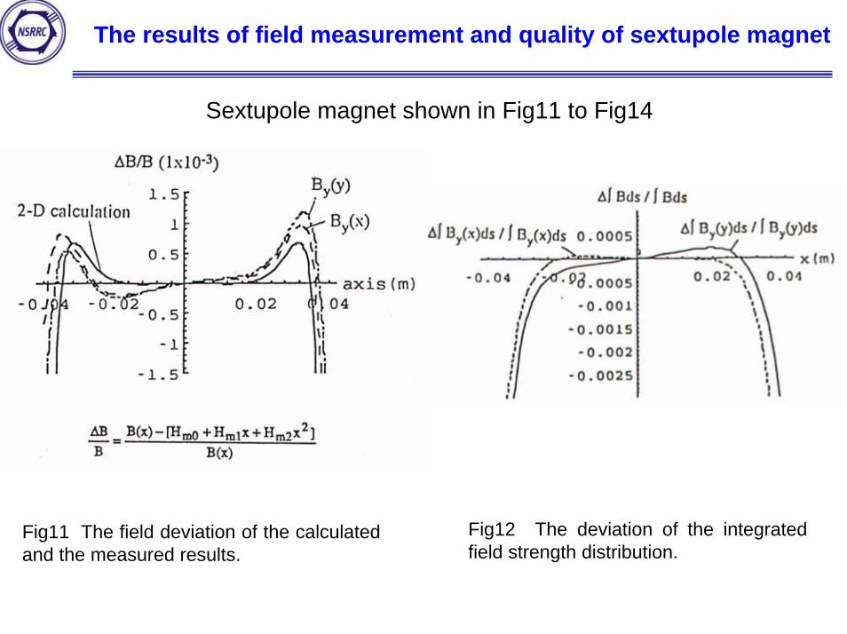
( ) ( )[ ] ( )xBxaaxBBB // 21 +−=∆

The results of field measurement and quality of SRRC magnet

Fig4 After and before 2-2 shims measurement results of the integrated field deviation

Fig3 The gradient field deviation of the 2-D calculation and measurement results at the magnetic center.

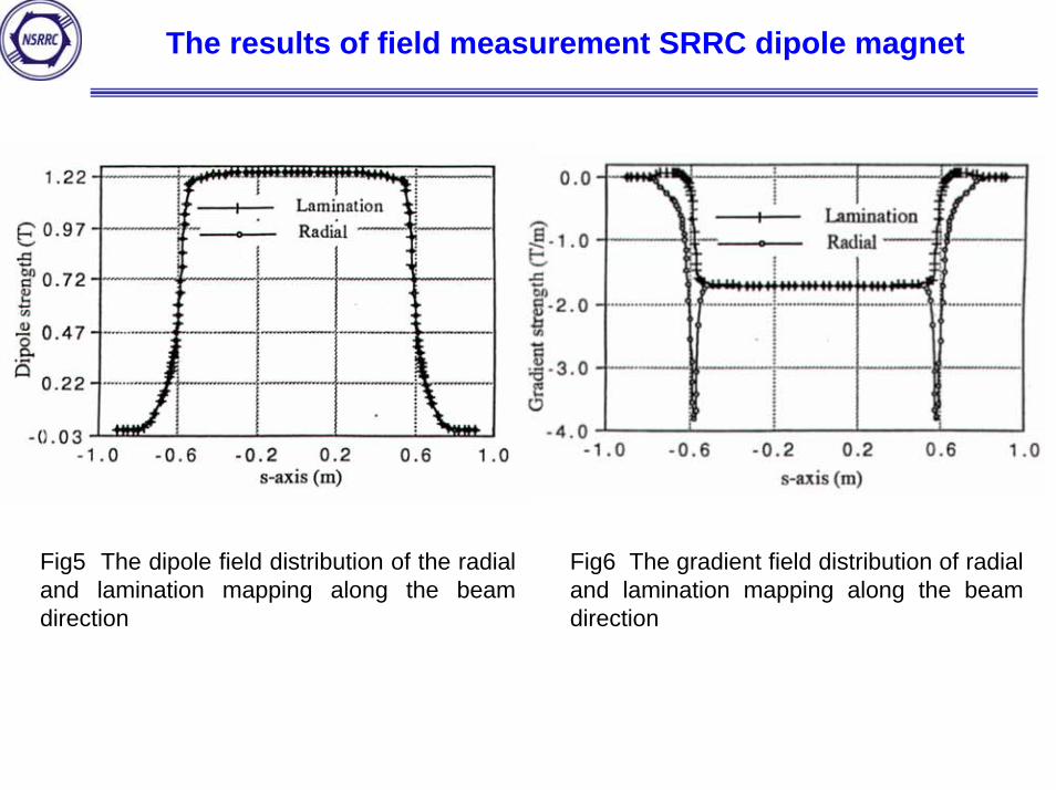
The results of field measurement SRRC dipole magnet

Fig5 The dipole field distribution of the radial and lamination mapping along the beam direction

Fig6 The gradient field distribution of radial and lamination mapping along the beam direction

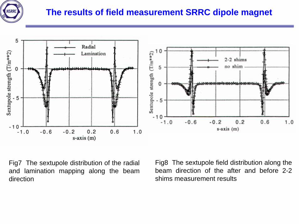
The results of field measurement SRRC dipole magnet

Fig8 The sextupole field distribution along the beam direction of the after and before 2-2 shims measurement results

Fig7 The sextupole distribution of the radial and lamination mapping along the beam direction

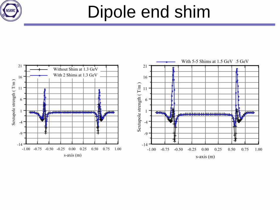
Dipole end shim

1.000.750.500.250.00-0.25-0.50-0.75-1.00-14

-9

-4

1

6

11

16

21Without Shim at 1.3 GeVWith 2 Shims at 1.3 GeV

s-axis (m)

Sext

upol

e st

reng

th (

T/m

)

1.000.750.500.250.00-0.25-0.50-0.75-1.00-14

-9

-4

1

6

11

16

21Without Shim at 1.5 GeVWith 5-5 Shims at 1.5 GeV

s-axis (m)

Sext

upol

e st

reng

th (

T/m

)

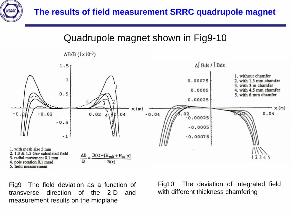
The results of field measurement SRRC quadrupole magnet

Quadrupole magnet shown in Fig9-10

Fig10 The deviation of integrated field with different thickness chamfering

Fig9 The field deviation as a function of transverse direction of the 2-D and measurement results on the midplane

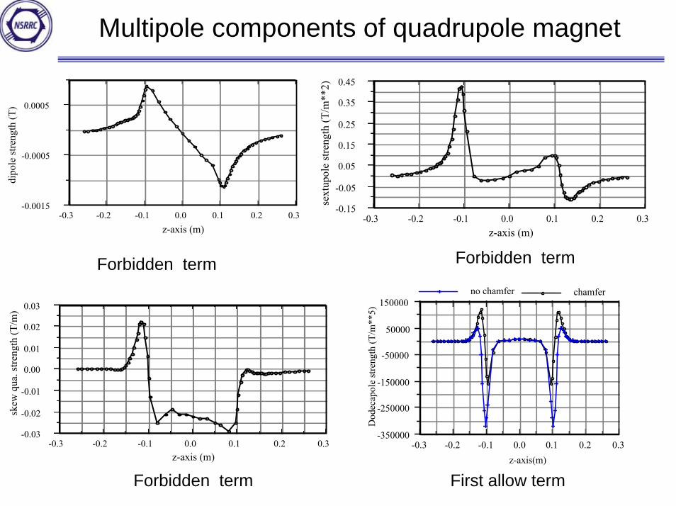
Multipole components of quadrupole magnet

0.30.20.10.0-0.1-0.2-0.3-0.15

-0.05

0.05

0.15

0.25

0.35

0.45

z-axis (m)

sext

upol

e st

reng

th (T

/m**

2)

0.30.20.10.0-0.1-0.2-0.3-0.0015

-0.0005

0.0005

z-axis (m)

dipo

le st

reng

th (T

)

0.30.20.10.0-0.1-0.2-0.3-350000

-250000

-150000

-50000

50000

150000chamferno chamfer

z-axis(m)

Dod

ecap

ole

stre

ngth

(T/m

**5)

0.30.20.10.0-0.1-0.2-0.3-0.03

-0.02

-0.01

0.00

0.01

0.02

0.03

Forbidden termForbidden term

z-axis (m)

skew

qua

. stre

ngth

(T/m

)

Forbidden term First allow term

The results of field measurement and quality of sextupole magnet

Sextupole magnet shown in Fig11 to Fig14

Fig12 The deviation of the integrated field strength distribution.

Fig11 The field deviation of the calculated and the measured results.

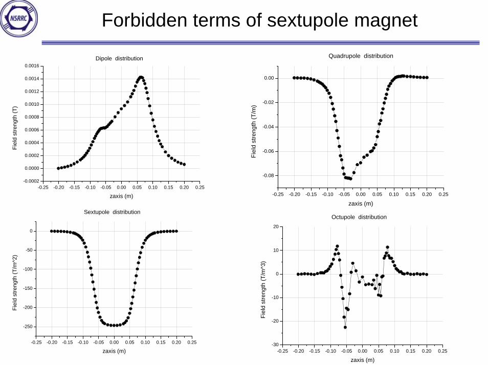
Forbidden terms of sextupole magnet

-0.25 -0.20 -0.15 -0.10 -0.05 0.00 0.05 0.10 0.15 0.20 0.25-0.0002

0.0000

0.0002

0.0004

0.0006

0.0008

0.0010

0.0012

0.0014

0.0016

Fiel

d st

reng

th (T

)

zaxis (m)

Dipole distribution

-0.25 -0.20 -0.15 -0.10 -0.05 0.00 0.05 0.10 0.15 0.20 0.25

-0.08

-0.06

-0.04

-0.02

0.00

Fiel

d st

reng

th (T

/m)

zaxis (m)

Quadrupole distribution

-0.25 -0.20 -0.15 -0.10 -0.05 0.00 0.05 0.10 0.15 0.20 0.25

-250

-200

-150

-100

-50

0

Fiel

d st

reng

th (T

/m^2

)

zaxis (m)

Sextupole distribution

-0.25 -0.20 -0.15 -0.10 -0.05 0.00 0.05 0.10 0.15 0.20 0.25-30

-20

-10

0

10

20

Fiel

d st

reng

th (T

/m^3

)

zaxis (m)

Octupole distribution

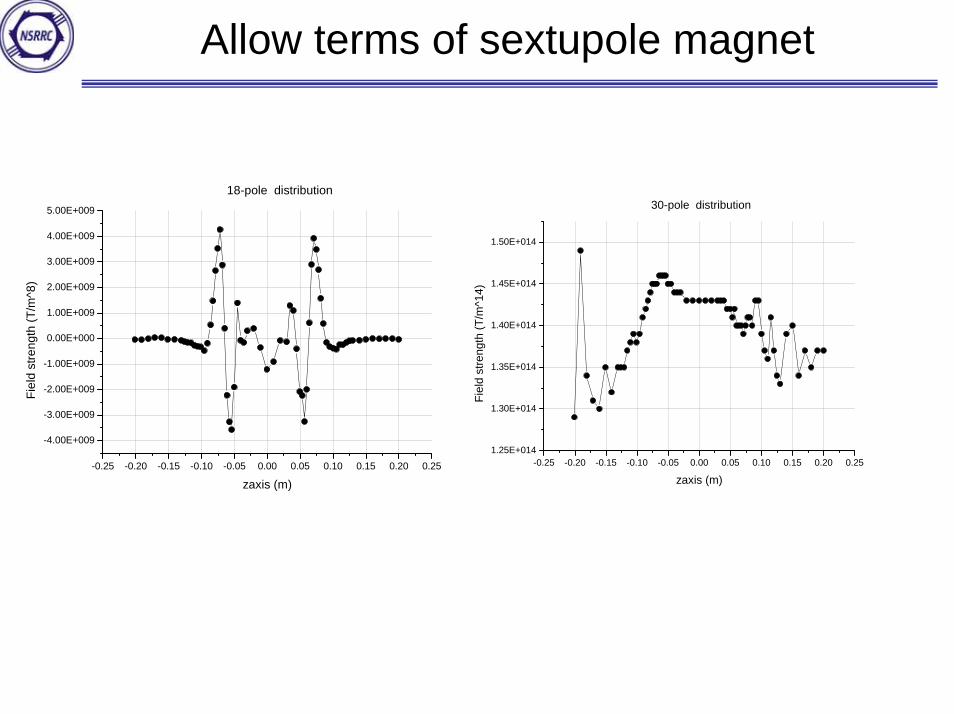
Allow terms of sextupole magnet

-0.25 -0.20 -0.15 -0.10 -0.05 0.00 0.05 0.10 0.15 0.20 0.25

-4.00E+009

-3.00E+009

-2.00E+009

-1.00E+009

0.00E+000

1.00E+009

2.00E+009

3.00E+009

4.00E+009

5.00E+009

18-pole distribution

Fiel

d st

reng

th (T

/m^8

)

zaxis (m)

-0.25 -0.20 -0.15 -0.10 -0.05 0.00 0.05 0.10 0.15 0.20 0.251.25E+014

1.30E+014

1.35E+014

1.40E+014

1.45E+014

1.50E+014

30-pole distribution

Fiel

d st

reng

th (T

/m^1

4)zaxis (m)

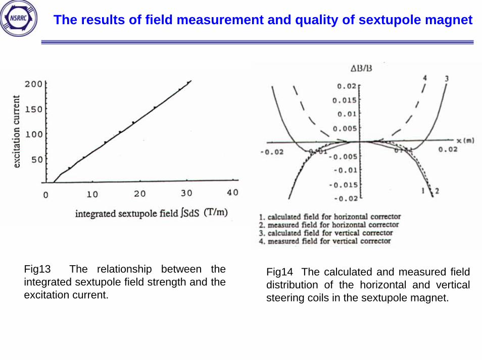
The results of field measurement and quality of sextupole magnet

Fig13 The relationship between the integrated sextupole field strength and the excitation current.

Fig14 The calculated and measured field distribution of the horizontal and vertical steering coils in the sextupole magnet.

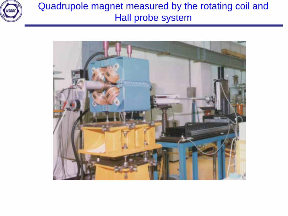
Quadrupole magnet measured by the rotating coil and Hall probe system

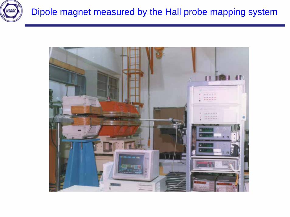
Dipole magnet measured by the Hall probe mapping system