Access to Credit and Role of Co-operation

Access to Credit and Role of Co-operation∗

Shamika Ravi†

Department of EconomicsNew York University

September 26, 2004

AbstractOne of the main advantages of having developed credit institutions is

that there are better opportunities for dealing with risk. When finan-cial institutions are not developed, alternate mutually beneficial arrange-ments evolve. Two examples of such arrangements are informal lendingand borrowing between friends and relatives and another is a co-operativesociety. This study is in two parts. First part looks at access to credit inrural India and second part compares how access to different risk sharingarrangements leads to differences in household response to risk. I am ableto do this by comparing data from two states of India ,Uttar Pradesh andKerala, that I collected. The results indicate that a) there are large dispar-ities in access to credit and particularly access to formal credit; b) thoughhouseholds in Kerala do not have better access to credit, the predictedprobability of borrowing from formal source is significantly higher (0.76)in comparison to Uttar Pradesh(0.2). Comparing five types of lenders, wefind that significance of banks and moneylenders are identical across tworegions. What drives the earlier result is the dependence on cooperativesin Kerala and informal ties with friends and relatives in UP. Both arerisk sharing arrangements that emerge from mechanism of co-operation.Part II evaluates the benefits and costs of institutionalizing co-operation.Using information on household responses to income shock we find that c)households with access to cooperative society are significantly less likelyto reduce consumption and input expenditure; d) they are more likely toget a larger fraction of loan approved; however, e) when a loan is rejected,households that rely on co-operatives, will borrow from more expensivealternative source like moneylenders while those that rely on informal tiesare likely to get another loan at the same cost elsewhere.

∗Draft†I am grateful to Jonathan Morduch for guidance and encouragement. I also wish to thank

Debraj Ray, Raquel Fernandez, Donghoon Lee and Deborah Levinson for helpful discussions;participants of seminars at New York University and NEUDC, Yale University, University ofMinnesota; GSAS, New York University for funding data collection; my survey team - JofyJoy, Sanoj Kumar, Sajai Ayyamkulam, Ramnish Baitha and Jai Prakash for all their helpand enthusiasm. Any remaining errors are my responsibility. All comments are welcome [email protected]

1

1 Introduction

Access to ready and available credit is an important factor in the economic

well being of a rural household. Perhaps one of the main advantages of having

developed credit institutions is that there are better opportunities to dealing

with risk. This is particularly relevant in rural communities. Opportunities for

personal savings in lesser developed communities are often restricted. However,

personal savings alone only offers limited potential for protection against risks of

fluctuating income. Therefore, there is reason to believe that other arrangements

for risk sharing can be mutually beneficial. A few examples of such mechanisms

are informal lending and borrowing amongst friends and relatives and more

organized cooperative societies. A household’s response to risk will depend on

the nature of arrangement that is available. Households that rely completely

on informal ties for financial assistance will respond differently to risk than a

household that is assured assistance through more organized mechanism. This

study is in two parts. In the first, I look at access to credit in rural India. In the

second part, I look at how access to different risk sharing arrangements leads

to differences in household response to risk. I am able to do this by comparing

two states of India ,Uttar Pradesh and Kerala.

Over the years, rural credit programs have become an integral part of govern-

ment policy in developing countries. Special banks for rural population were set

up in countries like India, Thailand and Philippines. Informal lenders, however,

still remain an important source of credit within villages. Bell and Srinivasan

(1986) show this for several states of India. While 84 percent of rural house-

holds in Bihar, India, rely only on informal sources for credit, even in a more

developed state like Punjab, this figure is as high as 46 percent. Institutional

credit, on the other hand, has been accused of bureaucratic rationing and biased

2

in favor of more educated and privileged households.1

Today, a typical rural credit ‘market’ in a less developed country comprises

of many lenders extending a variety of forms of credit. Alongside public lending

institutions like banks and cooperative societies, there is also a thriving informal

sector where private transactions occur under standard or personalized terms.

Indeed the economics of these two broad categories of credit are quite different.

Several features of an existing rural credit infrastructure are determined by

the way that borrowing households sort among different sources of credit. A

full understanding of the existing credit situation requires knowledge of the

preferences of the heterogeneous households within rural areas. First objective

of this paper is to study the nature and extent of household’s demand and

access for credit within a rural economy. We assess the strength and direction

of different factors that influence an agrarian household’s demand for credit.

In order to do so, we look at a wide spectrum of variables that a borrowing

household takes into consideration in it’s borrowing decision. We study three

kinds of loans 1) production loans 2) consumption loans and 3) medical loans.

It is necessary to include non-producation loans because they form a significant

proportion of rural household borrowing.

Unlike in the previous literature, informal creditors are not treated as a ho-

mogeneous entity. There are three broad informal sources of credit to rural

households: 1) professional moneylenders 2) traders, landlords and employers

and 3) neighbors and relatives. Each have distinct characteristics and provide

credit under varying terms and conditions. Professional moneylenders generally

provide credit against collateral and charge regular monthly interest payments.

Credit from traders, landlords and employers is based on some economic rela-

tionship that the borrower shares with the lender. The loans are either interest

1Dreze, Lanjouw and Sharma (1997)

3

free or at a nominal rate. But typically they involve collateral payment, which

could be in the form of future crops, labor time or future salary. The third cat-

egory, neighbors and relatives, is a major source of credit for rural households.

These loans are based on personal contacts and are generally interest free and

without collateral.

We develop an equilibrium model of sorting based on a random utility ap-

proach. Building on McFadden’s (1978) discrete choice framework, we allow

borrowers to have preferences for a wide variety of attributes of a contract, for

example, the source of loan and nature of collateral. Household preferences are

allowed to vary with household characteristics.

Not surprisingly, the results indicate that a) there are large disparities in

access to credit and particularly access to formal credit across households. But

somewhat more surprising is that while households in Kerala do not have sig-

nificantly better access to credit, the predicted probability of a household bor-

rowing from formal source is significantly higher (0.76) in comparison to Uttar

Pradesh(0.2). When we compare across five categories of lenders, we note that

predicted probabilities of borrowing from a bank and a moneylender are iden-

tical across two regions. But what drives the earlier result is the dependence

on cooperative societies in Kerala and informal ties with friends and relatives

in Uttar Pradesh. Both are risk sharing arrangements that emerge from mech-

anism of cooperation. While a cooperative society is an institutionalized form

of cooperation, friends and relatives are an informal form of cooperation. The

second part of this paper answers two following questions: a) Are there any ben-

efits to forming a cooperative society rather than dealing informally with other

households? and b) What are the costs, if any of institutionalization? Using

information on household responses to an income shock we find that households

that have access to cooperative society are significantly less likely to reduce

4

consumption and input expenditure. When households apply for loan, in re-

sponse to the income shock, they are likely to get a larger fraction of the loan

approved when they borrow from cooperative than when they rely on informal

ties. However, faced with a rejection, households that rely on co-operatives, can

only borrow from more expensive alternative sources like moneylenders. While

households that borrow from friends and relatives are likely to get another loan

at the same cost elsewhere.

The plan of the paper is as follows. Section 2 describes in some detail survey

methodology and data on which this study is based. Section 3 lays out some

summary statistics. In section 4 we discuss an appropriate model of household

borrowing decision. Section 5 looks at the estimation strategy and section 6 has

the first set of results for access to credit. In section 7, we have a discussion.

Section 8, has the next set of results for ’Responses to risk’ and the last section

9 has concluding remarks.

2 Data

The study is based on an original and comprehensive primary data set that

was compiled from a household survey. The survey covered 720 rural house-

holds from 21 villages across two districts in India and was held from June to

September 2002. Survey districts are from two diverse states Kerala and Uttar

Pradesh (U.P.). We deliberately picked two separate regions of the country to

study differences, if any, in the borrowing behavior of rural households.

Insert F igure1

Kerala is an average income state with per capita income of $254 per annum,

while Uttar Pradesh is a low income state with per capita income of $158 per

annum.2. The distinction between these two states becomes more stark when2Handbook 2001 - Select socio-economic indicators, Department of Statistics, Government

5

done along social development indicators. U.P. is termed as one of the ‘sick’

states of India (BiMaRU) and Kerala is ranked the highest based on social

indicators.

Insert Table1

Districts covered in survey are primarily agrarian where the population de-

pends either directly on cultivation or agriculture related jobs like daily wage

labour and trading. The sample district from U.P. is Kannauj and sample

district from Kerala is Palakkad.A district in India is divided into several devel-

opment blocks, which are then subdivided into many villages. For our sample,

we picked one representative block in each district, based on socioeconomic in-

dicators provided by District Statistics Office of each district. Incidentally both

sample blocks are also the largest in their respective districts. The sample block

in Uttar Pradesh has a total population of 2,14,964 and comprises of 108 vil-

lages. All villages are grouped into 78 panchayats. Panchayat is the lowest rung

in the democratic ladder with an annual budget and an elected governing body.

In Kerala, the sample block has a total population of 2,37,679 and comprises of

94 villages (wards) that are grouped into 9 panchayats.

Insert Table2

Villages from each block were chosen based on stratified random sampling.

In U.P., to pick a representative sample of households we stratified all 108 vil-

lages into 6 groups along three categories: a) distance from nearest metallic

road b) Muslim village c) scheduled caste village. While distance from nearest

metallic road serves as a good instrument for access to organized credit market,

it also is a very good proxy for access to organized labor market. Based on this

distance parameter, we form 4 groups. The second category is an important

of India.

6

one because interaction of Muslim households in the informal credit sector has

several distinct characteristics. For example, borrowing and lending amongst

Muslim households is done free of interest charges. This is similar to Udry’s

findings in northern Nigeria (1990). Stratification of villages along ‘Scheduled

Caste and other Backward Caste’ is important because these are target villages

for government programs. For example there are exclusive projects for employ-

ment, education, building roads, drainage system, housing and repair for these

villages. From each of the six categories for stratification, we randomly picked

two villages. We therefore have a total of 12 villages from U.P.. In Kerala, vil-

lages can not be distinguished based on religion and every village in the selected

block is linked with metallic road. There are, however, special grade panchayats

based on the population of scheduled caste and other backward castes. There

are two such panchayats in our selected block. We decided to include all the

9 panchayats in the block to get the most representative sample of households.

We therefore, randomly picked one village from each of the 9 panchayats. The

total number of villages covered in our sample is thus 21.

Village wise details of demographic and socioeconomic characteristics are

available in table 3. Ferozpur and Bahsuia are the two ‘schedule caste’ villages

in U.P. sample. The two muslim villages are Garaulli and Nisthaulli. In Kerala

the sample block has two schedule caste villages and we have surveyed both,

Vadakkencherry and Alathur.

Insert Table3.

To select households within a village, we obtained the voters’ list from the

last election, which was held in 2000. This is a reliable and exhaustive list that

has names of every member of a household above 18 years of age in the village.

From the list we randomly chose 30 households from each selected village in

U.P. and 40 households from each selected village in Kerala. Therefore we have

7

a total of 720 households in our sample, 360 each from Kerala and U.P.

To better understand household behavior with regards to indebtedness, we

separately look at a) current outstanding loans of the household as well as b)

loans that were repaid in the last two years. The purpose of this distinction is

two fold. Firstly to measure the extent of default of institutional and informal

loans and more importantly to gauge a household’s attitude towards default. To

analyze whether the source of credit affects a household’s perception of default.

Secondly this distinction helps analyze the repayment behavior of a household.

The data provides detailed household level information on several variables.

Member-wise household demographic details, primary and secondary occupation

and wage details are available. We also have detailed account of landholding,

cultivable land, usage, housing and asset holding - agricultural and household

assets. The data primarily focuses on the borrowing information of households.

Lending and saving data is available. Details of monthly expenditure and annual

income by source is also available.

Household response to risk looks at the household behavior in ’the worst

period in last 4 years’. The cause of the shock is known, in order to differentiate

whether it’s an aggregate or idiosyncratic one. We gathered information on

household’s response to overcome this shock. We have detailed information on

whether the household cut consumption expenditure, input expenditure, sell

jewelry, get an additional job, migrate for work etc. Besides these, we also

have data on whether the household sought any financial help. The sequence

in which they approached different lenders. We have lender-wise details on

number of loans applied and approved. Also, consequence of not getting a loan

or sufficient amount.

For the purpose of this study, the household survey data has been supple-

mented by panchayat and district level data provided by the Department of

8

Economics and Statistics, governments of U.P. and Kerala.

3 Some basic statistics

In this section we look at some of the basic findings from the data. First, we

discuss the village-wise nature of indebtedness, where we provide household level

information on amount and source of debt. In the second subsection, we briefly

explain the degree of presence and main characteristics of major lenders within

each village. In the last subsection, we look at the different purposes for which

rural households demand credit.

3.1 Indebtedness at a glance

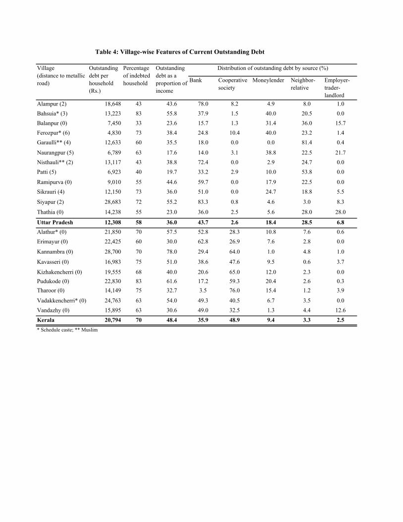
Village wise indebtedness information is available in table 4. Some interesting

facts emerge at the first glance. There is higher indebtedness in Kerala, whether

measured in terms of the amount of money borrowed per loan, or the debt to

income ratio per household, or even just the number of households per village

that have at least one current outstanding loan.

Insert Table4.

Table 4 also shows the break-up of debt by source. We should also mention

that on comparing the different sources of credit, we note that while house-

holds in both regions, depend to a large extent on banks for credit, there are

fewer number of loans taken from banks. As against from cooperative societies

in Kerala and neighbors-relatives in U.P., where households not only borrow

significant amounts, but the frequency is also higher from these sources.

3.2 Lenders - main characteristics and presence

There are two types of institutional credit available to the people in U.P. and

Kerala. They are banks and cooperative societies. The banks are either commer-

9

cial or specialized such as State Development Bank and Regional Rural Bank.

Natures of banks are similar in both the states. This is because the general

guidelines are established by National Bank for Agriculture and Rural Devel-

opment (NABARD). The cooperative societies, too follow the basic guidelines

set by NABARD, however, they acquire distinct regional characteristics. Once

registered, the cooperative gets linked to District Cooperative Bank which in

turn is linked to the State Cooperative Bank. These societies require member-

ship within a specified territorial area. In U.P., co-operatives remain primarily

agricultural. All loans, except ‘crop loans’ are seasonal and in kind, the most

common being fertilizers and seeds. Membership requires landholding. The co-

operatives also run specific projects of the local government which are targeted

towards scheduled caste/tribe or for households that lie below “poverty line”.

Under these projects, assistance is provided for self employment. In Kerala,

however cooperative societies have emerged as the backbone of rural credit in-

frastructure. Membership are typically based on occupation. There are tailors’,

weavers’, toddy-tappers’ and even unemployed people’s societies among others.

All cooperative societies have total functional autonomy3. He also audits the

accounts of the cooperative annually. Except against deposit and personal se-

curity, all other loans are given to members only. Deposits are of various kinds

but mostly gold, insurance policy, promissory certificate, government security

and debenture certificates. When a loan is taken, both parties - borrower and

the cooperative society, agree to a repayment schedule. But incase of failure to

comply with the agreed schedule, there is recasting of a new schedule.

Insert Table5

There are basically five private sources of credit to households. They are: a)

3The state appoints a registrar whose approval is required for any change in the rules andby-laws of the society.

10

professional moneylenders, b) traders, c) employers, d) landlords and e) neigh-

bors and relatives. Professional moneylenders are typically jewelers. There are

no eligibility restrictions and moneylenders provide credit to anyone who can

make collateral payment. The rate of interest they charge is monthly and de-

pends on the collateral which is commonly gold or silver. It is higher if no

collateral is placed. There are four cases in the data where previous defaulters

have received loans against new collateral4 . Traders give loans in the beginning

of a season, against future crops but in rare cases also provide consumption

loans. Landlords generally provide credit at nominal interest rates. There are

only two instances in the data where loans taken from landlord are of an “in-

terlinked” nature. Employers as a source of credit can be divided into two

types. Firstly, there are households that are employed in ‘regular’ jobs and earn

monthly salaries. These households have security of employment and can bor-

row from employer. The second type are landless households that are engaged

in casual labor for a daily wage. The economics of these two types are very

different. The final category, ‘neighbors and relatives’ are a significant source of

credit to households in U.P. The rate of interest charged is typically zero and

eligibility depends on social and personal ties between the households.

Insert Table6

3.3 Type of loan by source

Here, we look at village-wise break up of the main types of loans, by the source.

A loans is classified as a ‘type’ based on the purpose for which it was taken.

There are many reasons why households borrow, but they can all be broadly

classified into three major groups - consumption, production and medical rea-

sons. Within ‘consumption loan’, the three major sub-categories for borrowing4This is because a moneylender gives loans worth 50 to 60 percent of the collateral value.

Only small borrowers who repeatedly default have difficulty acquiring new loans.

11

are a) ceremonies and marriages; b)purchase of durables like T.V. and bicycle;

c) day-to-day consumption and d) education. The second type of loan, ‘produc-

tion loan’ comprises of a) purchase of machinery and equipment; b) purchase of

inputs like fertilizer and seeds; c) purchase of livestock d) business investment

and d) construction. The third loan type is ‘medical loan’. We look at this cat-

egory separately because it is a type of ‘emergency’ borrowing when households

behave differently and it is also a major category in the data.

Insert Table7

Table 7 shows that in both U.P and Kerala, more than one third the total

credit is borrowed for consumption and medical expenses. This is a sizeable

amount and suggests that in order to study the borrowing behavior of rural

households we need to also consider loans other than for production purposes. A

careful look at the break-up reveals that in Kerala, most of the non-production

loans are for consumption requirement, in U.P., one-third of this is to meet

medical needs. In terms of number of loans taken, consumption and medical

loans account for more than production loans, which suggests that amounts

borrowed for consumption and medical purposes are lower, but are taken at

greater frequency in both the regions.

4 Borrowing decisions of households

In this section we analyze the decision process of a borrowing household. Within

this, we look at a borrowing household’s choice of lender and see if it is influ-

enced by the type of loan. We begin the analysis by setting out an equilibrium

model of rural credit market. We first describe the main component of this

model, a discrete choice framework that governs each households borrowing de-

cisions. Following McFadden(1973, 1978), I use a discrete choice framework

12

to study the household’s choice of lender as this provides a natural way to

estimate heterogeneous preferences for different types of credit. The utility

function specification is based on the random utility model developed by Mc-

Fadden(1978) and the specification of Berry, Levinsohn and Pakes(1995), which

includes choice-specific unobservable characteristics. We treat each loan as a

separate borrowing decision.

4.1 Borrower’s optimization problem

The structure considered is as follows: agents first decide whether to borrow or

not, and if they decide to do so, they choose whom to borrow from. The utility

from borrowing a loan is V il which is given by:

V il = αilLl − αirrl + ηl + εil if V i

l > 0 (1)

and V il = 0 otherwise.

In the model, a borrowing household chooses a lender l to maximize it’s

utility, which depends on the observable and unobservable characteristics of his

choice. Let Ll represent the observable characteristics of loan L taken from

lender l, other than the rate of interest that vary with the households borrow-

ing decisions and let rl denote the rate of interest. Observable characteristics of

a loan include loan amount, collateral offered, type of loan (whether consump-

tion, production, medical etc.), repayment frequency and when it was taken.

Household i’s optimization problem is given by :

Maxl

V il = αilLl − αirrl + ηl + εil (2)

where ηl is the unobserved quality of lender corresponding lender. This could

include reputation of the lender, enforcement techniques, renegotiation possi-

bilities, time spent in procuring the loan, bribe, travelling time and expense

13

etc. The last term εil is an idiosyncratic error term that captures unobserved

variation in household i’s preference for a particular lender.

Each household’s valuation of choice characteristics is allowed to vary with

it’s own characteristics Hi including landholding, income, occupation, educa-

tion, age households composition and sex of household head. The parameters

associated with loan characteristics and rate of interest αij for j ∈ {L, r} areallowed to vary with households own characteristics,

αij = α0j +XXx=1

αxjHix. (3)

Equation (3) describes household i’s valuation for choice characteristics j.

The first term captures the taste for the choice characteristics that is com-

mon to all households and the second term captures observable variations in

the valuation of these choice characteristics across households with different so-

cioeconomic characteristics. This heterogeneous specification of the coefficients

allows for variation in preferences across different types of households.

The above specification of the utility contains two stochastic components

that allow flexibility in explaining the observed data. The first component is

the lender specific unobservable ηl. This term captures the common value of

unobserved aspects of a particular lender that is , value shared by all households.

Because many loan and lender attributes are likely to be unobserved in any data

set, the specification avoids biases due to unobserved lender characteristic.

The second stochastic component of the utility function is the idiosyncratic

term εil , which is assumed to be additively separable from the rest of the utility

function. We assume a Weibull distribution, which gives rise to the multinomial

logit model. With this assumption, the probability that household i selects

lender l , P il is given by

P il =

exp(αilLl − αirrl + ηl)Pk exp(α

iLLk − αirrk + ηk)

(4)

14

where k indexes all possible lenders.

The multinomial logit assumption implies that the ratio of the probabilities

between any two choices is independent of the characteristics of the remaining

set of alternatives (Independence of Irrelevant Alternatives assumption). This

is usually not a very good assumption to make but in this specification of the

utility function the impact of IIA is weakened since there are heterogeneous

coefficients.

4.2 Equilibrium

The random utility specification is not only flexible from an empirical point of

view, but also has a relevant theoretical interpretation. Without the idiosyn-

cratic error component εil this specification would suggest that two households

with identical characteristics would make identical borrowing decisions. This is

unlikely to be true, a useful interpretation of εil is that it captures unobserved

heterogeneity in preferences across the otherwise identical households. Thus, for

a set of households with a given set of observed characteristics, the model pre-

dicts not a single choice but a probability distribution over the set of borrowing

choices. We use Nash equilibrium concept.

Household i chooses lender l if utility that it gets from this exceeds the utility

from all other possible loan choices.

V il > V i

k =⇒W il + εil > W i

k + εik =⇒ εil − εik > W ik −W i

l ∀ k 6= l (5)

where W il includes all the non-idiosyncratic components of the utility function

V il . As this shows the probability that a household chooses a particular lender

will depend on the characteristics of all the possible loans. In this way , the

probability that household i chooses lender l can be written as a function of

loan characteristics, both observed and unobserved, prices and households char-

15

acteristics:

P il = f(Hi, L, r, η). (6)

5 Estimation

Having specified the theoretical framework, we now move on to the estimation

procedure of the model. Let us rewrite the equation function as described in

equation (2) and (3) as the following:

V il = φl + θil + εil (7)

where, φl is the choice specific constant, θil is the interaction term that includes

all parts of the utility function that interact household and choice characteristic

and εil is the idiosyncratic error term. Therefore,

φl = α0lLl − α0rrl + ηl (8)

and

θil =

"XXx=1

αxlHix

#Ll −

"XXx=1

αxrHix

#rl. (9)

Here, choice specific constant φl denotes the portion of utility provided by

lender l that is common to all households. The unobservable component ηl of

this constant denotes the unobserved preferences for lender l that is correlated

across households while εil represents unobserved idiosyncratic preferences over

and above the shared component.

5.1 Estimation procedure

For any combination of interaction parameters and loan specific constants, the

model predicts the probability that each household i chooses lender l

P il =

exp(φl + θil)Pk exp(φk + θik)

. (10)

16

Maximizing probability that each household makes a correct borrowing de-

cision, conditioning on the full set of observed household characteristics, Hi and

choice characteristic {Ll, rl}, gives rise to the following log-likelihood function

=Xi

Xl

Iil ln(Pil ), (11)

where Iil is an indicator variable that equals 1 if household i chooses lender l in

the data and 0 otherwise. The first order condition is the derivative of the log

likelihood function above with respect to φl and θil .5

6 Results (I): Access to Credit

Before we look at the results, it is helpful to see the variables in the regres-

sion. We have four sets of controls. Household characteristics, loan characteris-

tics, lender dummies and variables that capture household’s credit relationships.

Household characteristics include various demographic, occupation and income

asset details. Loan characteristics include size, length, usage and collateral de-

tails. The credit relationship variables include whether there is a co-op in the

village, whether the household has any savings deposit in a formal institution,

whether the household has ever borrowed to repay old debts, or has repaid late.

The number of moneylenders in the village and the distance to the nearest bank.

Also during the ’worst period in last 4 years’, did the household apply for loan,

but didn’t get any. And if the household didn’t need to apply for a loan.

From table 8, we can see that while Kerala households have higher annual

income, households in U.P. have larger asset holdings. Assets include household

and agricultural assets, and value of house. The average land holding is signifi-

cantly higher in U.P. In terms of years of education, Kerala, on average, has 2.35The derivative of the log likelihood function with respect to φl :

δ

δφl=Xi=l

δ ln(P il )

δφl+Xi6=l

δ ln(P il )

δφl=Xi=l

¡1− P i

l

¢+Xi 6=l

¡−P il

¢= 1−

Xi

¡P il

¢

17

more years of education. Kerala households are smaller with fewer dependents.

Occupational distribution indicates that most U.P. households are cultivators

while half of Kerala households are casual laborers. Kerala has higher unem-

ployment levels.

Loan characteristics indicate that Kerala borrows larger loans for longer

periods, most likely against collateral and for consumption purposes. Number

of households that borrow in order to repay old debts are higher in U.P. Same

is true for late repayment. On an average, most Kerala loans are borrowed from

cooperative societies while most loans in U.P. are borrowed from friends and

relatives.

Insert Table8

To assess a households ’access to credit’, we have only considered households

that have applied for loan at least once in the last two years. Of course this

leaves out households that would ’self select’ themselves out of the credit market.

However, the probability of this should be very low as we have considered all

forms of lenders including neighbors, relatives and friends where the incidence of

’self selection’ are low. As specified before, an unit of observation here is a loan.

So households that do not borrow or borrow at most once, appear once, but

households that borrow more than once are included for each loan. I haven’t

differentiated across these two types. 6 So, the household decision is of two

stages. First, decide whether to borrow or not, and if they decide to borrow,

they choose a lender. Now, in our specification, we have looked at all 5 lenders

simultaneously. However, to begin with, we will look at them as two categories

- formal and informal. Formal lenders include banks and cooperative societies.

Informal lenders include moneylender, neighbor-relative and trader-landlord-

6Siamwalla et. al. (1993) also have the same strategy.

18

employer. The first set of results obtained from Heckman probit estimation are

presented in Table 9. After this we will look at the predicted probabilities from

the multinomial logit that we run for all five lenders simultaneously following

our model.

Insert Table9

Table 9 is the result from Heckman probit regression. First of all, rho is

significant, which is evidence for selection. So, access to credit also affects

choice of lender. In the ’access to credit’ column, the dependent variable take

value 1 if the household has a current outstanding loan and 0 if it does not.

The dependent variable in second column is type of lender. It equals 1 if source

is formal. and 0 if informal. Now, to accurately measure ’access’ to credit, we

only look at households that have applied for loan at least once in the last two

years.

The results indicate that access to credit is dependent on household charac-

teristics like total income, total asset holding and total number of members in

the household. Higher income and owning more assets increases a household’s

access to credit, but does not affect the choice of lender. This could be because

more assets imply more possible collateral. Higher education does not affect ac-

cess but improves access to formal sources of credit. This corroborates findings

of Dreze, Lanjouw and Sharma (1997) that formal credit is biased in favor of

more educated households. Access to credit improves significantly with number

of household members but reduces with number of dependents. This implies

that higher the number of earning members in the household, better the access.

Female headed households have significantly lower access to credit, but the type

of lender is not affected by gender of head. Households that belong to the back-

ward community, as defined by government, have greater access to credit, but

significantly to informal sources. Muslim households too have greater access to

19

credit but have lower chances of borrowing from formal sources. Both these

results might be driven from the fact that loans taken from informal sources

are smaller and with greater frequency. Except for casual labor households that

are more likely to borrow from informal sources, type of credit is not affected

by occupation. Access, however is affected by occupation. Households that are

unemployed have significantly lower access while those with a secure salaried

job have greater access to credit. This is not surprising, as secure employment

with regular flow of income implies greater repayment capacity.

Being in Kerala does not lead to greater access to credit for a household,

but significantly increases chances of borrowing from formal sources. What’s

interesting is that presence of a cooperative society as well as the number of

moneylenders in the village increases the access to credit, significantly. Also not

surprisingly, households that have savings account in formal institution have

better access. What’s surprising, however, is that the distance to bank from

village increases the access to credit but not significantly to formal credit. This

is perhaps because when banks are further, households take several smaller loans

from other sources. Households that have borrowed to repay old debts and those

that have repaid late tend to have better access, but to informal sources.

Insert F igure2

Now we will look at results for all types of lenders simultaneously. Follow-

ing our specification we run a multinomial logit for lender choice. Here the

dependent variable takes 5 discrete values from 1 to 5, for each lender type.

Coefficients of a multinomial logit regression are difficult to interpret. This is

because there are multiple equations and the coefficients are relative to the base

category. In our estimation, we keep ’not borrow’ as an option. All coefficients

are relative to ‘not borrow’ outcome. Rather than concentrate on the structural

20

interpretations of the estimated coefficients, we concentrate instead on the pre-

dictions of the model. Figure 2 shows the predicted probabilities for each lender

from this estimation. I have presented the predicted probabilities against the

log of total wealth of a household. Wealth includes the annual income and total

asset owned, both of which affect access to credit significantly, as we saw from

results in table 9. The median wealth level is higher in Uttar Pradesh.

Figure 2 shows the predictions from our model controlling for household char-

acteristics, loan characteristics and households credit relation characteristics.

It clearly shows the difference in credit infrastructure between the two states.

Equally remarkable, however, are the similarities between the two states. When

we compare the two most evaluated sources of credit - banks and moneylenders,

we note that the predicted probability of borrowing from a bank increases with

total wealth in both states. The probability of borrowing from a moneylender

decreases with wealth in both states. This reflects the similarity in the relative

importance of these two institutions as sources of credit, across different regions.

The predicted probabilities also imply that Kerala households across different

wealth levels rely on cooperative societies for credit. While, in Uttar Pradesh,

households across different wealth levels rely on informal ties with neighbors

and relatives for credit. Based on the formal-informal break up of lenders, the

predicted probability of a formal source is 0.76 in Kerala and 0.2 in U.P.

7 What do the results imply?

The results imply that despite the presence of specialized rural banks and local

moneylenders, households largely depend on mutual risk sharing arrangement

of cooperation. In Kerala, the nature of cooperation is institutionalized in the

form of cooperative societies. In Uttar Pradesh, the nature of cooperation re-

mains informal between neighbors and relatives. One interesting aspect to study

21

would be the emergence of these different institutions What leads to institution-

alization of a mechanism - here cooperation? This would require information

on the institutions themselves as well as historical data. We have neither, and

therefore will concentrate on the benefits and costs of institutionalization of

cooperation. Are there benefits to forming a cooperative society rather than

dealing informally with other households? And what are the costs, if any?

There are several potential explanations for the emergence of diverse insti-

tutions in different regions. Kerala has always been a ’special’ state due to it’s

extraordinary achievements in education and health. Dreze and Sen (2002) sug-

gest that Kerala’s success is the result of public action that promoted extensive

social opportunities and the widespread, equitable provision of schooling, health

and other basic services. On the other hand, they attribute failures of Uttar

Pradesh to the public neglect of these very same opportunities.

Let’s first compare the two separate risk sharing arrangements that have

evolved in Kerala and U.P. From the results it is evident that in both regions,

households primarily resort to similar mechanisms of cooperation. Making use

of local information and enforcement, co-operatives can diminish the adverse

selection and moral hazard problems that exist within financial systems. Given

private information, low monitoring costs and enforcement possibilities, the

same is true for informal arrangements between friends and relatives. Based

on earlier work, we can claim that there is sufficient evidence to suggest the

significant presence of risk sharing arrangements between individuals. One ex-

ample is Rosenzweig (1988) based on ICRISAT data that looks at intrafamilial

transfers. Other works include Townsend (1995) which looks at implications of

risk sharing in southern India and in rural Thailand. Study by Udry (1994)

looks at informal credit institutions in northern Nigeria, which involve lending

and borrowing arrangements between friends and relatives. Hoff (1994) looks

22

at informal risk sharing.

To validate our claim that co-operatives and neighbors-relatives perform

similar roles in the credit market of the two samples, we present some more

results. The household decision is now whether to borrow from the risk sharing

arrangement or other sources like moneylenders, banks etc. If the household

decides to borrow from the risk sharing arrangement, it then decides whether

to borrow from a cooperative society or from informal ties. The result of the

Heckman probit estimation are for this are in Table 10.

Insert Table10

The dependent variable in ’Cooperation’ regression takes value 1 if household

decides to borrow from the risk sharing arrangement and 0 otherwise. The

dependent variable in the ’Form of Cooperation’ regression takes value 1 if

household borrows from a cooperative society and 0 if household borrows from

friends and relatives. The results indicate that household characteristics do

not affect the form of risk sharing arrangements that the household chooses to

borrow from. Number of years of education leads to lower participation in risk

sharing arrangements. This would be because more educated households have

comparatively better opportunities outside the community. Households from

backward communities are less likely to borrow from co-operatives and friends

and relatives. This is because as a community they have fewer opportunities

and as a result mutual risk sharing or borrowing and lending is not feasible.

These households rely on moneylenders and other formal of informal credit.

Households that have repaid late are most likely to hold loans from cooperative

societies rather than friends and relatives. Well, this is because repayment

schedule is formally defined in a cooperative set up and therefore being ’late’

in repayment is an observable factor. While amongst friends and relatives,

23

repayment schedules are often not fixed.

Most importantly, being in Kerala significantly increases the probability of

borrowing from a cooperative society.

8 Results (II): Response to Risk

We know that households in the two samples mostly rely on different forms of

cooperation arrangements. In this section, we will analyze if there are benefits to

institutionalizing the mechanism of cooperation. That is, we will try to answer

the two following questions: a) Are there any benefits to forming a cooperative

society rather than dealing informally with other households? and b) What are

the costs, if any of institutionalization?

For this analysis, we will use information on household responses to an in-

come shock. And see if access to different risk sharing arrangement has any

effect on their response. We have information on ’Worst financial period for

household in the last 4 years’ for each household. We also know the type of

shock, whether it was aggregate, that affected the entire village like drought or

flood; or an idiosyncratic one, like disease or death. For each household in our

sample, we have detailed information on the responses to this shock. We also

have data on whether the household sought any financial help. The sequence

in which they approached different lenders. We have lender-wise details on the

amount of loan the household applied and the amount that was approved. We

also look at the consequences of being rejected a loan or only getting insuffi-

cient amount. Figure 3 gives a distribution of household responses following an

income shock. The most common response was to cut consumption expendi-

ture. This includes among others, taking kids out of school and spending less

on food and fuel. Dissaving by selling jewelry and withdrawing from deposit

was also common response. Monetary and non monetary help from neighbors

24

and relatives is also a common response.

Insert F igure3

To study the impact of access to different risk sharing mechanisms, we look

at three of the commonly stated response: a) cut consumption b) cut input

expenditure and c) get additional job. We present the results of the first two.

Table 11 shows the estimation results. The dependent variable in regression

’Reduce consumption’ takes value 1 if the household stated that it had to cut

expenditure in response to the income shock, and 0 if not. The dependent

variable in regression ’Spend less on inputs’ takes value 1 if household stated

that it reduced expenditure on inputs in response to the income shock and

0 if not. The control variables are household characteristics, credit relations

characteristics, interaction of access to cooperative with household occupation

and interactions of access to friends and relatives with household occupation.

Insert Table11

The results indicate that households that have access to cooperative societies

are less likely to reduce consumption as well as spend less on inputs. Households

that borrow from neighbors and relatives are more likely to reduce consumption

and input. Farmers, casual labor and unemployed households are significantly

likely to reduce expenditure on consumption in response to an income shock.

However, when they have access to credit from a cooperative society, they are

significantly less likely to reduce consumption. Backward community house-

holds have a higher likelihood of reducing consumption and input after a shock,

but when they have access to cooperative credit, they are significantly less likely

to do so. Richer household are less likely to cut consumption and so are house-

holds with regular salaried employment, which is not surprising as they have

25

better insurance opportunities. Households that have a savings account in for-

mal institution are also significantly less likely to cut consumption as well as

reduce input expenditure. This is because they have opportunities to self insure

by dissaving. Presence of a cooperative society reduces probability of cutting

inputs but increases chances of cutting consumption. This result is not sur-

prising. Remember that the co-operatives in Uttar Pradesh are agricultural

co-operatives that provide cheap seeds and fertilizer, two of the main inputs on

which households spend money. Number of moneylenders in the villages reduces

the likelihood of cutting consumption and input after a shock. Distance to bank

has no impact on either responses.

The results in table 11 establish that access to institutionalized risk sharing

arrangement affects household response to income shock. The benefits are re-

flected in the fact that households are less likely to cut consumption and input

expenditure merely due to access to this source of credit.

Now we will try to see benefits of institutional cooperation by analyzing

whether the financial needs of a household, after an income shock, are better met

through co-operatives or informal networks. Here, we use data on what fraction

of the loan that the household asked for was approved by the lender. The result

of this is in the first column of table 12, under ’Loan approved/applied’. We

estimate this using OLS methods. The dependent variable is ratio of amount

received to total amount applied.

Insert Table12

The results indicate that households with access to cooperative society are

likely to get a larger fraction of the loan applied while those who borrow from

neighbors and relatives are likely to get smaller fraction. SC-ST households

get significantly smaller fraction of loan asked, but those with access to co-

26

operatives get a significantly larger fraction. The same is true for farmers as

well. Households with savings account get a smaller fraction of loan approved.

Households with larger asset holdings get larger fraction approved. This might

be due to their ability to keep collateral. But households with higher income

get smaller fraction approved.

What is the effect of a household getting rejected for a loan, either completely

or partially? When asked, two of the most common response was ’Borrow from

another source at higher interest’ and ’Borrow from another source at same

interest’. The second column in table 12 show the results of a probit estimation.

The dependent variable takes the value 1 if the household borrowed from another

source at higher interest rate and 0 if the households borrowed from another

source at same interest rate.

The results are completely surprising. When a loan is rejected, households

that borrow from cooperative society are significantly likely to borrow from

another source at much higher interest rate. While households that borrow from

friends and relatives are likely to get another loan at the same cost elsewhere. On

comparing the coefficients on occupations we note that farmers, self employed

and casual labor will borrow from another source at same interest rate. However,

if they borrow from co-operatives, and are rejected, then they will have to borrow

from another source at much higher interest rate. When unemployed households

get rejected for a loan, they get loan from another source at very high interest

rate. If rejected, SC-ST households will have to borrow at higher interest rate,

regardless of access to co-operatives.

These results imply that there are costs of institutionalization of cooperation.

When a household gets rejected for a loan from a neighbor or relative, it is

most likely going to get one from another source at the same cost. But when

households that borrow from co-operatives, are rejected for a loan, they only

27

have costlier alternatives like moneylenders. One likely explanation would be

that when a cooperative society is formed in a community, it erodes the older

networks and informal ties.

So institutionalization of a risk sharing mechanism such as mutual coop-

eration has benefits and costs. The benefits are manyfold. Households that

have access to a cooperative are less likely to reduce consumption or production

expenditure when faced with an idiosyncratic income shock. This is because

access to a cooperative guarantees to some degree ready and available credit in

times of need. It is also likely that the household receives a larger fraction of

the loan it applies from a cooperative society. Households that rely on informal

ties with neighbors and relatives are more likely to get rejected in full or par-

tially when they ask for a loan. Also these households are less insured against

income shocks as we notice that they are more likely to reduce consumption

and input expenditure as a result of a shock. However, in the face of rejection,

they are more likely to get a loan from another source without paying higher

interests. Households that rely on co-operatives as a risk sharing arrangement,

however, can only get loan from another source that is costlier. In most cases,

these are moneylenders. So, it would seem that when communities formalize

this arrangement, it replaces the older networks and informal ties.

9 Conclusion

Access to ready and available credit is an important factor in the economic

well being of a rural household. Perhaps one of the main advantages of having

developed credit institutions is that there are better opportunities to dealing

with risk. This is particularly relevant in rural communities. Opportunities for

personal savings in lesser developed communities are often restricted. However,

personal savings alone only offers limited potential for protection against risks of

28

fluctuating income. Therefore, there is reason to believe that other arrangements

for risk sharing can be mutually beneficial. A few examples of such mechanisms

are informal lending and borrowing amongst friends and relatives and more

organized cooperative societies. A household’s response to risk will depend on

the nature of arrangement that is available. Households that rely completely

on informal ties for financial assistance will respond differently to risk than a

household that is assured assistance through more organized mechanism. This

study is in two parts. In the first, I look at access to credit in rural India.

In the second part, I compare the risk responses of households with access to

different risk sharing arrangement and compare the benefits and costs of these

different arrangement. I am able to do this by comparing two states of India

,Uttar Pradesh and Kerala.

The main results indicate that a) there are large disparities in access to credit

and particularly access to formal credit across households. But somewhat more

surprising is that while households in Kerala do not have significantly better

access to credit, the predicted probability of a household borrowing from formal

source is significantly higher (0.76) in comparison to Uttar Pradesh(0.2). When

we compare across five categories of lenders, we note that predicted probabilities

of borrowing from a bank and a moneylender are identical across two regions.

But what drives the earlier result is the dependence on cooperative societies in

Kerala and informal ties with friends and relatives in Uttar Pradesh. Both are

risk sharing arrangements that emerge from mechanism of cooperation. While

a cooperative society is an institutionalized form of cooperation, friends and

relatives are an informal form of cooperation. The second part of this paper

answers two following questions: a) Are there any benefits to forming a coop-

erative society rather than dealing informally with other households? and b)

What are the costs, if any of institutionalization? Using information on house-

29

hold responses to an income shock we find that households that have access

to cooperative society are significantly less likely to reduce consumption and

input expenditure. When households apply for loan, in response to the income

shock, they are likely to get a larger fraction of the loan approved when they

borrow from cooperative than when they rely on informal ties. However, faced

with a rejection, households that rely on co-operatives, can only borrow from

more expensive alternative sources like moneylenders. While households that

borrow from friends and relatives are likely to get another loan at the same cost

elsewhere.

30

References

[1] Banerjee, A., Timothy Besley, and Timothy Guinnane, "Thy neighbor’s

Keeper: The Design of a Credit Cooperative with Theory and a Test",

Quarterly Journal of Economics, May 1994

[2] Bell, C. T.N. Srinivasan, and C. Udry (1997) “Rationing Spillovers and

Interlinking in Credit Markets : The Case of Rural Punjab”, Oxford Eco-

nomic Papers, 49, 557-585.

[3] Bell, C. (1990), “Interactions Between Institutional and Informal Credit

Agencies in Rural India”, The World Bank Economic Review, Vol. 4, No

3, 297-328.

[4] Berry, S., J. Levinsohn, and A. Pakes (1995) “Automobile Prices in Market

Equilibrium,” Econometrica, Vol.63, No 4, 841-890.

[5] Dreze, J , P. Lanjouw and N. Sharma (1997) “Credit in Rural India: A

case Study”, The DERP 6, STICERD, LSE.

[6] Kochar, A. (1997) “An Empirical Investigation of Rationing Constraints in

Rural Credit Markets in India”, Journal of Development Economics, Vol.

53, 339-371

[7] Maddala, G.S. (1983). Limited Depdendent and Qualitative Variables in

Econometrics. Econometrics Society Monographs, No.3. Cambridge Uni-

versity Press.

[8] McFadden, D. (1973) “Conditional Logit Analysis of Qualitative Choice

Behaviour,” in Frontiers of Econometrics, ed. by P.Zarembka. New York:

Academic Press.

31

[9] McFadden, D. (1978). “Modelling the Choice of Residential Location,” in

Spatial Interaction Theory and Planning Models, ed. by A. Karvist, et al.

Amsterdam: North Holland, 75-96.

[10] Ray, Debraj (1998) Development Economics. Princeton University Press.

[11] Rosenzweig, Mark, "Risk, Implicit Contracts and the Family in Rural Ares

of Low-Income Countries", Economic Journal, 1988.

[12] Hoff, K. and J.E. Stiglitz (1990) “Introduction : Imperfect Information and

Rural Credit Markets - Puzzles and Policy Perspectives”, The World Bank

Economic Review, Vol. 4, No 3, 235-250.

[13] Udry, C. (1990) “Credit Markets in Northern Nigeria : Credit as Insurance

in a Rural Economy”, The World Bank Economic Review, Vol. 4, No 3,

251-270.

[14] Department of Statistics, Government of India, (2001), Handbook 2001.

32

Figure 1: Map of India - outline of states

Kannauj – Uttar Pradesh Palakkad – Kerala

Kerala Uttar Pradesh India

Per capita income (Rs.) 17756 9261 15887Population density (per sq. k.m.) 749 473 274Sex ratio (women per 1000 men) 1058 902 933Rural literacy (%) 91 50 57Female school enrolment rate (6-17 years) 90.8 61.4 66.2Male school enrolment rate (6-17 years) 91 77.3 77.6Total fertility rate (per woman) 1.96 3.99 2.85Infant mortality rate (per 1000 live births) 16.3 86.7 67.6Source: Selected Socio-economic Indicators 2001, Department of Statistics, Govt. of India; Handbook of Statistics, R.B.I; National Family and Health Survey-2, 1998-99

Table 1: Basic Socio-Economic Characteristics

Table 2 : Sampling Methodology

4 groups2 villages from each group

= 8 villages(240 households)

Nearest metallic road(access to formal credit)

(access to organised labour market)

2 villages(60 housholds)

Muslim village(interest free loans)

2 villages(60 households)

Schedule caste/tribe village(special govt. assistance)

Stratification Criteria

Village name (distance to metallic road)

Main occupation Per-capita landholding (acres)

Per-capita Income

(Rs/year)

Highest education per household

Alampur (2) F, RJ 0.46 6,234 12th grade

Bahsuia* (3) F,CL 0.19 4,352 10th grade

Balanpur (0) F, CL, SE, RJ 0.155 5,440 10th gradeFerozpur* (6) CL, F, SE 0.1 1,997 8th gradeGaraulli** (4) F, CL, SE 0.45 4,820 8th grade

Naurangpur (5) F 0.27 5,564 10th gradeNisthauli** (2) F, CL, SE 0.33 4,276 8th grade

Patti (5) F, CL, SE, RJ 0.22 5,880 8th gradeRamipurva (0) CL,F 0.23 2,872 10th gradeSikrauri (4) F, RJ, CL 0.27 3,758 10th gradeSiyapur (2) F, SE 0.24 5,601 10th gradeThathia (0) F, RJ, SE, CL 0.21 6,923 12th grade

Uttar Pradesh 0.26 4,810Alathur* (0) CL, SE, RJ, F 0.09 7,398 10th gradeErimayur (0) CL, RJ, SE, F 0.17 13,489 12th gradeKannambra (0) CL, RJ, SE, F 0.12 9,631 10th gradeKavasseri (0) RJ, SE, CL, HW, F 0.14 8,426 12th gradeKizhakencherri (0) CL, RJ, F, SE 0.31 11,584 12th gradePudukode (0) CL, RJ, SE, HW 0.14 10,083 10th gradeTharoor (0) CL, SE, RJ, F 0.08 7,401 10th gradeVadakkencherri* (0) RJ, CL, SE, HW 0.06 11,401 10th grade

Vandazhy (0) RJ, CL, SE, F 0.12 12,336 10th grade

Kerala 0.14 10,194 44

* Schedule caste; ** Muslim; F=farmer; CL=casual labour; SE=self employment; RJ="regular job" (with montly salary and security of employment); HW=headload worker (with permit)

333545

55

45484544

1128

1243

3

10023

27313

11

Percentage of household with atleast one regular job

13

3

Table 3: Village-wise Basic Demographic and Socio-economic Characteristics

Bank Cooperative society

Moneylender Neighbor-relative

Employer-trader-landlord

Alampur (2) 18,648 43 43.6 78.0 8.2 4.9 8.0 1.0Bahsuia* (3) 13,223 83 55.8 37.9 1.5 40.0 20.5 0.0Balanpur (0) 7,450 33 23.6 15.7 1.3 31.4 36.0 15.7Ferozpur* (6) 4,830 73 38.4 24.8 10.4 40.0 23.2 1.4Garaulli** (4) 12,633 60 35.5 18.0 0.0 0.0 81.4 0.4

Naurangpur (5) 6,789 63 17.6 14.0 3.1 38.8 22.5 21.7Nisthauli** (2) 13,117 43 38.8 72.4 0.0 2.9 24.7 0.0Patti (5) 6,923 40 19.7 33.2 2.9 10.0 53.8 0.0

Ramipurva (0) 9,010 55 44.6 59.7 0.0 17.9 22.5 0.0Sikrauri (4) 12,150 73 36.0 51.0 0.0 24.7 18.8 5.5

Siyapur (2) 28,683 72 55.2 83.3 0.8 4.6 3.0 8.3

Thathia (0) 14,238 55 23.0 36.0 2.5 5.6 28.0 28.0

Uttar Pradesh 12,308 58 36.0 43.7 2.6 18.4 28.5 6.8Alathur* (0) 21,850 70 57.5 52.8 28.3 10.8 7.6 0.6Erimayur (0) 22,425 60 30.0 62.8 26.9 7.6 2.8 0.0

Kannambra (0) 28,700 70 78.0 29.4 64.0 1.0 4.8 1.0

Kavasseri (0) 16,983 75 51.0 38.6 47.6 9.5 0.6 3.7

Kizhakencherri (0) 19,555 68 40.0 20.6 65.0 12.0 2.3 0.0Pudukode (0) 22,830 83 61.6 17.2 59.3 20.4 2.6 0.3Tharoor (0) 14,149 75 32.7 3.5 76.0 15.4 1.2 3.9

Vadakkencherri* (0) 24,763 63 54.0 49.3 40.5 6.7 3.5 0.0Vandazhy (0) 15,895 63 30.6 49.0 32.5 1.3 4.4 12.6

Kerala 20,794 70 48.4 35.9 48.9 9.4 3.3 2.5* Schedule caste; ** Muslim

Table 4: Village-wise Features of Current Outstanding Debt

Village (distance to metallic road)

Outstanding debt per household (Rs.)

Percentage of indebted household

Outstanding debt as a proportion of income

Distribution of outstanding debt by source (%)

Village (distance to metallic road)

Number of moneylenders in village

Distance to nearest bank (kms.)

Bank Name Number of cooperative societies

Alampur (2) 4 4 AB 1

Bahsuia* (3) 2 7 AB 0Balanpur (0) 4 6 BoI 1Ferozpur* (6) 0 8 BoI 0Garaulli** (4) 0 2 AB 0

Naurangpur (5) 1 3 BoI 0

Nisthauli** (2) 2 1 AB 0

Patti (5) 0 6 AB 0

Ramipurva (0) 0 2 AB 0Sikrauri (4) 3 3 BoI 0

Siyapur (2) 2 3 BoI 0

Thathia (0) 12 1 AB, BoI 1

Uttar Pradesh 3 3.83 0.25

Alathur* (0) 12 2 CB 13

Erimayur (0) 5 2 NB, CB, SBT 2

Kannambra (0) 10 2.5 SBT, CB 2

Kavasseri (0) 6 3 SBT, CB 1

Kizhakencherri (0) 5 5 VB, CB 5Pudukode (0) 4 2.5 CB, SBT 2

Tharoor (0) 5 4 SBT, CanB, CB 3

Vadakkencherri* (0) 6 2 SBT, CB 1

Vandazhy (0) 3 1 CB, VB 4

Kerala 6.22 2.67 3.67

Table 5: Village-wise Creditors' Information

* Schedule caste, ** Muslim; AB= Allahabad Bank; BoI= Bank of India; CB= Commercial Bank; SBT= State Bank of Travancore; CanB= Canara Bank; VB= Vijaya Bank; NB= National Bank

Land title (77)None (13)

Land title (50)None (25)Future crop (17)None (80)Gold, silver (9)Land title (7)None (81)Land title (10)Gold, silver (4)None (50)Future crop (35)

Land title (45)Gold, Silver (32)None (22)Gold, Silver (59)Land title (33)

None (6)

None (53)Gold, silver (36)Land title (8)None (60)Gold, silver (20)Land title (20)None (45)Gold, silver (30)Guarantor (10)

Moneylenders

Neighbors-Relatives

Employer-Landlord-Trader

60 to 120

Banks

Co-operative societies

10 to 16

12 to 15 Half yearly

Monthly

Not fixed

Not fixed

* Remaing forms of collateral: Provident Funds, Guarantor, Bank deposit and Labor hours

Whether household falls in tartget group, against bank deposits, jewelry, immovable propertyMembership, deposits, guarantor; some loan categories - self employment, education, marriage, house repair, religious rites, medical, job search in foreign countriesNone, as long as collateral is provided; commonly addressed as "blade loans"

Social ties or personal relationship with lender

Economics ties with lender

Neighbors-Relatives

*Collateral requirements (%)

Eligibility conditions and special characteristics

Credit source Typical Range of interest rates (%/ )

*Collateral requirements (%)

Eligibility conditions and special characteristics

0 to 60

0 to 60

Credit source Typical Repayment frequency

Moneylenders

* Remaing forms of collateral: Provident Funds, Guarantor, Bank deposit, Labor hours and Livestock and land cultivatiob rights

Usually based on scheme; falling below "poverty line", "backward caste" or size of land holdingMembership based on size of landholding; these are agr co-ops; all loans except 'crop loans' are in kindNone, as long as collateral is provided; previous defaulters get credit against new collateral; (loan/collateral) value is 60%

Social ties or personal relationship with lender

Economics ties with lender

Banks 10 to 18

Half yearly

Table 6: Synoptic List of Main Credit Sources- Uttar Pradesh

Table 6: Synoptic List of Main Credit Sources- Kerala

Typical Repayment frequency

Employer-Landlord-Trader

12 to 20

60 to 240

0

0 to 144

Typical Range of interest rates (%/ )

Co-operative societies

Not fixed

Half yearly, some annual

Depending on loan type; 'Gold loans'-monthlyMonthly

Not fixed

Amount (Rs.) Number Amount (Rs.) Number Amount (Rs.) Number

Alampur 51,000 5 362,900 10 0 0Bahsuia 158,496 12 211,700 25 26,500 5Balanpur 130,002 6 28,500 2 65,000 5Ferozpur 32,304 16 70,004 11 42,588 13Garaulli 208,800 16 29,205 9 129,000 10Naurangpur 74,000 8 32,800 10 20,202 3Nisthauli 62,000 8 317,508 12 14,000 2Patti 85,704 8 112,005 9 10,000 4Ramipurva 38,997 9 140,503 11 700 1Sikrauri 23,200 4 294,789 33 46,503 9Siyapur 23,500 4 410,004 12 9,800 2Thathia 114,000 8 414,000 20 41,502 6Uttar Pradesh 1,002,003 104 2,423,918 164 405,795 60Alathur 304,000 20 569,997 27 0 0Erimayur 349,998 6 532,004 22 5,000 2Kannambra 607,992 28 339,003 9 185,999 11Kavasseri 112,806 18 483,506 23 83,000 5Kizhakencherri 188,689 19 567,996 26 22,500 5Pudukode 355,500 18 550,706 26 5,000 2Tharoor 187,250 35 351,696 16 27,000 4Vadakkencherri 283,500 15 678,996 18 28,002 3Vandazhy 317,604 14 272,704 16 5,000 2Kerala 2,707,339 173 4,346,608 183 361,501 34

Table 7: Village-wise Break up of Types of Loan

Consumption Production Medical loan Village

Mean Std.Dev. Sample size Mean Std. Dev. Sample size

Household Characteristics

Logarithm of annual income 9.73 1.65 332 10.3 0.98 359

Logarithm of total assets 11.76 1.61 332 11.6 1.35 359

Total landholding 1.8 2.38 332 0.62 1.24 359

Number of years of education 5.2 0.9 332 7.4 0.73 359

Age of household head 49.9 14.32 332 55.44 12.2 359

Total number of members 7.6 4 332 4.8 2.2 359

Number of dependents 2.9 2.11 332 0.57 0.92 359

Female headed household 0.11 0.311 332 0.15 0.34 359

SC_ST 0.18 0.38 332 0.22 0.42 359

Muslim 0.18 0.38 332 0.15 0.32 359

Farmer 0.68 0.46 332 0.14 0.34 359Self employed 0.04 0.19 332 0.11 0.31 359

Casual labor 0.22 0.41 332 0.51 0.49 359

Regular salaried job 0.06 0.23 332 0.2 0.4 359

Unemployed 0.01 0.09 332 0.03 0.17 359

Loan characteristics

Logarithm of size of loan 8.45 1.3 341 9.1 1.22 397

Length of loan 1.95 2.9 341 2.02 2.59 397

Use of collateral to secure loan 0.41 0.49 341 0.79 0.4 397

Collateral==land 0.12 0.32 341 0.22 0.42 397

Collateral==jewelry 0.03 0.155 341 0.32 0.47 397

Collateral==future crop 0.03 0.15 341 0 0 397

Collateral==guarantor 0.015 0.12 341 0.02 0.14 397

Loan use =production 0.48 0.47 341 0.4 0.44 397

Loan use=consumption/medical 0.49 0.43 341 0.6 0.49 397

Credit relations

Co-operative society in village 0.1 0.3 332 0.97 0.14 359

Savings account in formal institution 0.33 0.47 332 0.38 0.47 359

Borrow to repay old debt 0.23 0.43 332 0.1 0.3 359

Late repayment 0.36 0.48 332 0.2 0.4 359

Number of moneylenders in village 1.9 6.9 332 6.4 4.8 359

Distance to nearest bank 3.9 2.5 332 2.3 1.4 359

Dummy (applied but got no loan) 0.06 0.24 332 0.02 0.14 359

Dummy (No apply) 0.15 0.35 332 0.21 0.41 359

Lender

Friends-relatives 0.4 0.48 341 0.05 0.22 397

Bank 0.16 0.37 341 0.22 0.43 397

Co-operative society 0.04 0.19 341 0.54 0.5 397

Moneylender 0.33 0.47 341 0.16 0.36 397

Employer-trdaer-landlord 0.07 0.25 341 0.03 0.16 397Sample size - 691 households and 738 loans

Table 8: Details and summary statistics of variables in regression

Uttar Pradesh Kerala

Coefficient z-stat Coefficient z-stat

Constant -1.561 (4.69)** -2.717 -0.9

Household CharacteristicsLogarithm of annual income 0.041 (2.06)* 0.003 0.06

Logarithm of total assets 0.05 (2.31)* 0.133 1.41

Number of years of education -0.078 -1.69 0.181 (1.98)*

Age of household head -0.002 -0.6 0.004 0.56

Total number of household members 0.043 (4.62)** -0.016 -0.4

Number of dependent members -0.072 -0.66 0.072 1.14

Female -0.147 (2.06)* -0.013 -0.06

SC_ST 0.346 (5.67)** -0.549 (4.82)**

Muslim 0.243 (2.48)* -0.363 -1.18

Farmer -0.203 -1.88 -0.205 -0.62

Casual labor -0.131 -1.28 -0.168 (2.17)*

Unemployed -0.721 (3.84)** 0.506 0.68

Regular salaried job 0.192 (4.27)** 0.138 0.28

Kerala dummy 0.267 0.432 0.463 (2.68)**

Credit Relations

Co-operative society in village 0.591 (3.50)** 0.28 0.8

Savings acount with formal institution 0.122 (2.33)* 0.034 0.23

Ever borrowed to repay old debt 0.772 (9.93)** -0.153 -0.24

Ever repaid late 0.16 (13.01)** -0.283 -0.39

Number of moneylenders in village 0.017 (4.19)** -0.005 -0.32

Distance to nearest bank 0.03 (2.39)* 0.012 0.27

Rho 0.925 0.0451

Observations

Wald

Log-likelihoodAbsolute value of z statistics in parentheses, *significant at 5%, **significant at 1%, The estimation is done using Heckman Probit method. The dependent variable in 'Access to Credit' probit regression takes value one if household has borrowed and 0 if not; In the 'Type of Lender' probit, dependent variable takes value 1 if the lender is formal and 0 if informal.

106.7

-2379.67

Table9: Selection Regressions - Access and Type of LenderAccess to Credit Type of Lender

990

0.2

.4.6

.8Pr

edic

ted

prob

abilit

y

8 10 12 14 16log (wealth)

N-R BankCoop Ml

Uttar Pradesh

0.2

.4.6

.8Pr

edic

ted

prob

abilit

y

8 10 12 14 16log (wealth)

N-R BankCoop Ml

Kerala


Constant -1.701 (2.89)** -2.879 -1.02


Logarithm of annual income 0.067 -1.78 0.048 -0.45

Logarithm of total assets 0.04 -1.01 -0.041 -0.4

Number of years of education -0.206 (3.32)** 0.084 0.39

Age of household head -0.001 -0.25 0.02 1.49

Total number of household members 0.028 1.69 -0.083 -1.86

Number of dependent members -0.052 -1.63 0.159 1.78

Female -0.209 -1.56 0.062 0.18

SC_ST -0.421 (3.70)** -0.293 -0.67

Farmer 0.427 (2.14)* -0.892 -1.14

Casual labor 0.373 1.95 -1.093 -1.46

Unemployed 0.352 0.99 -0.94 -0.96

Regular salaried job 0.035 0.16 -0.973 -1.22

Credit Relations

Co-operative society in village 0.182 0.76 0.669 0.81

Savings acount with formal institution 0.127 1.34 -0.395 -1.57

Ever borrowed to repay old debt 0.018 0.15 0.131 0.41

Ever repaid late 0.066 0.6 0.817 (2.36)*

Number of moneylenders in village 0.007 1.06 0.013 0.9

Distance to nearest bank 0.035 1.61 0.13 (2.07)*

Kerala dummy 0.442 1.76 3.489 (5.18)**

Rho 0.0739 1.071

Observations

Wald

Log-likelihoodAbsolute value of z statistics in parentheses, * significant at 5%; ** significant at 1%; Dependent variable in "cooperation" regression takes value 1 if household borrows either from co-operative or from friends and relatives and 0 otherwise; Dependent variable in "form of co-operation" takes value 1 if household borrows from co-operative and 0 if household borrows from friends and relatives.

-683.729

Co-operation Form of co-operationTable10: Regression for forms of co-operation- co-operative soicety or informal ties

104.07

990

Figure3: Household Response to Income Shock

0 50 100 150 200 250 300

cut consumption

sell jewelry

additional job

monetary help(nr)

nonmonetary help(nr)

borrow co-op

borrow village ML

cut input expenditure

withdraw deposit

borrow outside ML

borrow trader

government help

Number of households


Constant 0.289 (2.12)* 2.264 (11.04)**


Log of total income -0.081 (9.77)** -0.013 -1.31

Log of total assets -0.012 -1.32 -0.118 (9.82)**

Number of years of education 0.061 (4.14)** 0.073 (3.97)**

Age of household head 0.002 (2.41)* -0.007 (6.51)**

Number of dependents/total members 0.174 (3.14)** 0.013 0.2

Female 0.068 (2.10)* 0.31 (7.32)**

SC_ST 0.004 0.12 0.232 (5.53)**

Farmer 0.284 (5.24)** -0.823 (6.30)**

Self employed - - -0.652 (4.63)**

Casual labor 0.196 (3.82)** -0.593 (4.66)**

Unemployed 0.37 (3.49)** -

Regular salaried job -0.889 (14.98)** -2.344 (10.90)**

Kerala dummy 0.378 1.62 -1.721 -1.84

Credit Relations

Co-operative society in village 0.292 (5.14)** -0.196 (3.12)**

Savings account in formal institution -0.205 (8.57)** -0.269 (8.14)**

Number of moneylenders in village -0.024 (10.81)** -0.004 -1.41

Distance to nearest bank 0.009 1.6 -0.011 -1.67

Co-operative and interactions

Borrow from Co-operative society -0.063 (2.41)* -0.353 (4.75)**

Co-op*SC_ST -0.594 (9.29)** -0.179 -1.74

Co-op*farmer -0.025 (2.28)* - -

Co-op*labor -0.388 (4.74)** -0.113 -1.22

Co-op*selfemp 0.244 (2.17)* -

Co-op*unempl - -

Co-op*job - 1.634 (8.00)**

Neighbors-Relatives and interactions

Borrow from Neighbors/relatives 0.228 1.39 1.63 (8.64)**

NR*farmer 0.498 (2.97)** -1.268 (6.57)**

NR*labor 0.214 1.25 -1.848 (9.26)**

NR*selfemp - -1.795 (7.06)**

NR*unempl -0.154 -0.58 -

NR*job 0.717 (3.60)** -

Observations 691 691

Adjusted R square 0.18 0.27

Table11: Response to Income Shock

(I) Reduce consumption (II) Spend less on inputs

Absolute value of z statistics in parentheses, * significant at 5%; ** significant at 1%; Regression(I) estimated using probit, dependent variable takes value 1 if household cut consumption after shock and 0 if not; Regression II estimated using probit, dependent variable takes value 1 if household reduced expenditure on inputs and 0 if not.


Constant 0.682 (16.81)** 7.891 (.)


Log of total income -0.008 (4.67)** -0.124 (7.41)**

Log of total assets 0.019 (9.00)** -0.005 -0.23

Number of years of education -0.01 (3.10)** 0.253 (7.73)**

Age of household head -0.001 (6.99)** -0.014 (7.86)**

Number of dependents/total members -0.08 (6.63)** 0.922 (7.91)**

Female -0.01 -1.3 0.917 (12.90)**

SC_ST -0.054 (7.47)** 0.382 (6.32)**

Farmer -0.014 -0.47 -6.479 (22.38)**

Self employed -0.069 (2.25)* -6.72 (23.62)**

Casual labor 0.006 0.19 -6.466 (24.19)**

Unemployed - - - -

Regular salaried job 0.046 -1.5 -5.576 (17.89)**

Kerala dummy 0.247 1.23 0.226 1.09

Credit Relations

Co-operative society in village -0.003 -0.25 -0.452 (5.28)**

Savings account in formal institution -0.021 (3.97)** -0.175 (3.75)**

Number of moneylenders in village 0 -1.09 -0.057 (12.34)**

Distance to nearest bank -0.011 (9.11)** -0.028 (2.74)**

Co-operative and Interactions

Borrow from Co-operative society 0.123 (3.24)** 0.78 (4.96)**

Co-op*SC_ST 0.043 (3.37)** 0.399 (2.79)**

Co-op*farmer 0.098 (2.52)* 1.21 (7.11)**

Co-op*labor -0.085 (2.20)* 1.91 (10.97)**

Co-op*selfemp -0.02 -0.49 - -

Co-op*unempl - - 6.568 (16.70)**

Co-op*job -0.174 - - -

Neighbors-Relatives and Interactions

Borrow from Neighbors/relatives -0.005 -0.12 -2.378 (15.87)**

NR*farmer -0.002 -0.04 1.223 (7.65)**

NR*labor -0.069 -1.47 - -

NR*selfemp 0.084 -1.53 - -

NR*unempl 0 (.) - -

NR*job 0.117 (2.29)* -0.714 (2.95)**

Observations 691 523

Adjusted R square 0.3 0.49Absolute value of t statistics (Regression I) and z statistics (Regression II) in parentheses, * significant at 5%; ** significant at 1%; Regression(I) estimated using OLS methods, dependent variable is loan amount approved to loan amount applied; Regression II estimated using probit, dependent variable takes value 1 if household had to borrow from another source at higher rate of interest and value 0 if at same rate of interest.

Table 12: Response to Income Shock in Credit MarketLoan Approved/Applied Consequence of Rejection

Documents

Access to Credit and Role of Co-operation