Finance and Economics Discussion SeriesDivisions of Research & Statistics and Monetary Affairs

Federal Reserve Board, Washington, D.C.

Accounting for Innovations in Consumer Digital Services: IT stillmatters

David Byrne, Carol Corrado

2019-049

Please cite this paper as:Byrne, David and Carol Corrado (2019). “Accounting for Innovations in Con-sumer Digital Services: IT still matters,” Finance and Economics Discussion Se-ries 2019-049. Washington: Board of Governors of the Federal Reserve System,https://doi.org/10.17016/FEDS.2019.049.

NOTE: Staff working papers in the Finance and Economics Discussion Series (FEDS) are preliminarymaterials circulated to stimulate discussion and critical comment. The analysis and conclusions set forthare those of the authors and do not indicate concurrence by other members of the research staff or theBoard of Governors. References in publications to the Finance and Economics Discussion Series (other thanacknowledgement) should be cleared with the author(s) to protect the tentative character of these papers.

Accounting for Innovations in Consumer

Digital Services: IT still matters

David Byrne∗ and Carol Corrado†‡

June 15, 2019

(Original Draft, March, 2017)

Abstract

This paper develops a framework for measuring digital services in the face of ongoinginnovations in the delivery of content to consumers. We capture what Brynjolfsson andSaunders (2009) call “free goods” as the capital services generated by connected consumers’stocks of IT digital goods; this service flow augments the existing measure of personal con-sumption in GDP. Its value is determined by the intensity with which households use theirIT capital to consume content delivered over networks, and its volume depends on thequality of the IT capital. Consumers pay for delivery services, however, and the comple-mentarity between device use and network use enables us to develop a quality-adjustedprice measure for the access services already included in GDP.

Our new estimates imply that accounting for innovations in consumer content deliverymatters: The innovations boost consumer surplus by nearly $1,800 (2017 dollars) per con-nected user per year for the full period of this study (1987 to 2017) and contribute morethan 1/2 percentage point to US real GDP growth during the last ten. All told, our morecomplete accounting of innovations is (conservatively) estimated to have moderated thepost-2007 GDP growth slowdown by nearly .3 percentage points per year.

Keywords: Consumer Digital Services; Information and Communication Technology; Con-sumer Durables; Consumer Surplus; Innovation; Digital Content Delivery; National Ac-counting, and Price Measurement

∗Board of Governors of the Federal Reserve System, Washington, D.C. The views expressed in this paper are those ofthe authors and do not necessarily reflect those of the Board of Governors or other members of its staff.

†The Conference Board and Center for Business and Public Policy, McDonough School of Business, GeorgetownUniversity. Corresponding author (cac289@georgetown.edu)

‡This paper was prepared for the NBER/CRIW Conference, “Measuring Innovation in the 21st Century,” GeorgetownUniversity, Washington, D.C., March 10-11, 2017. We have benefited from presentations of this paper at the 5th IMFStatistical Forum in Washington, D.C. (November 2017), the ESCoE Measurement Conference in London (May 2018)and the 5th World KLEMS Conference in Cambridge, Mass (June 2018). We received no financial support for this paper.

1 Introduction

Capturing the impact of innovations in consumer content delivery in conventional well-being measures,

e.g., GDP, presents significant challenges. It also seemingly requires a new approach because the

manifestation of these innovations in consumer welfare (e.g., time spent consuming high quality content

via networked IT devices) does not involve a market transaction at the time of consumption, which

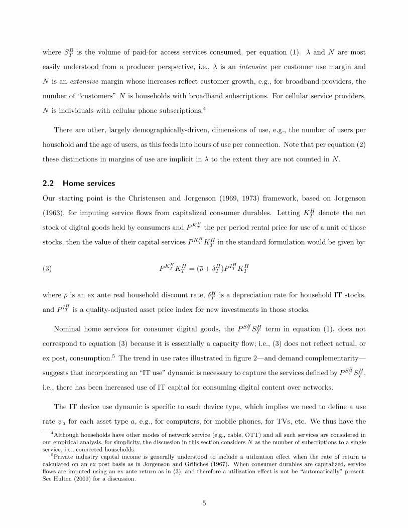
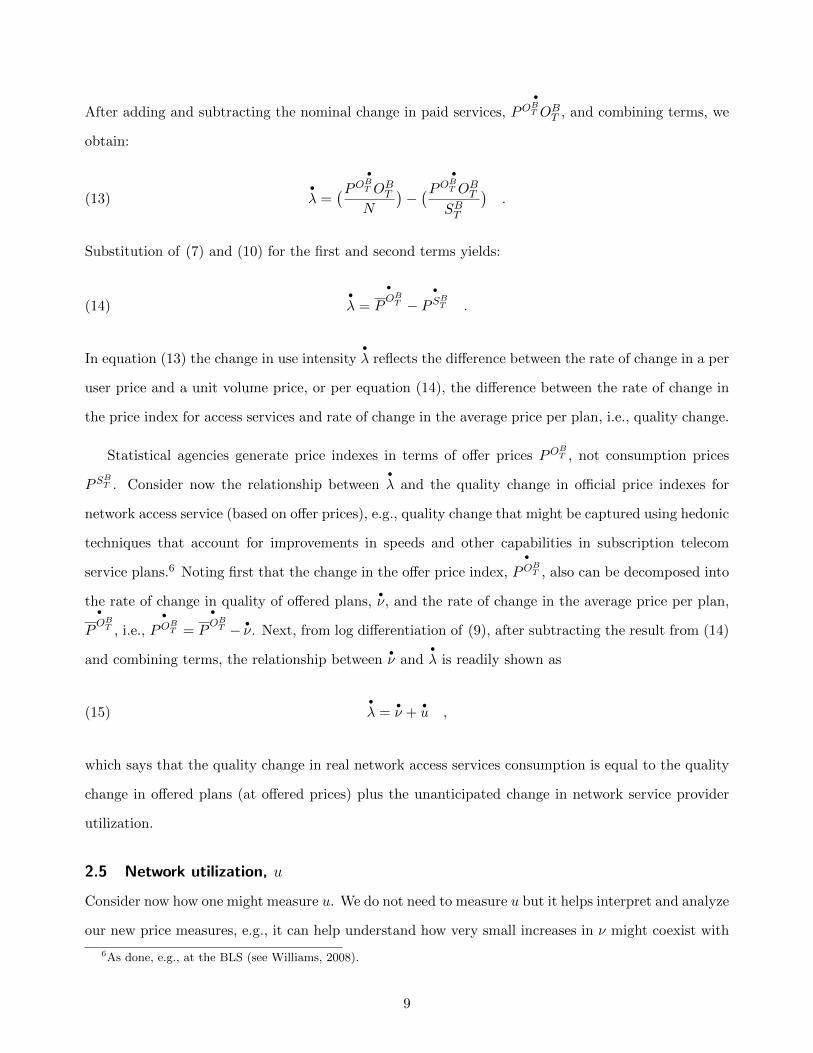
is where price collectors/estimators look to pick up new goods as they appear. Figure 1 shows that

innovations in consumer content delivery have been very rapid since the turn of this century, suggesting

their impacts may be missed in existing GDP; indeed, they are clustered in the mid-2000’s when the

slow down in the trend GDP growth emerged. Is it possible that the substitution of uncounted,

so-called free goods for purchased counterparts is a culprit in this much-discussed slowdown?

This paper adapts a not-so-new approach—capitalization of consumer digital goods—to address

this question, but the standard approach is augmented with an accounting for how IT devices and

subscription network access services are used and consumed.1 To understand why a use-adjusted

version of an “old” approach is both (a) needed and (b) up to the task of capturing 21st century

innovations, consider first that it is consumer-owned devices with advanced processing technology—

computers, powerful smartphones, smart TVs, and video game consoles—that enable the consumption

of high quality content in many homes (and elsewhere), and these services currently are uncounted in

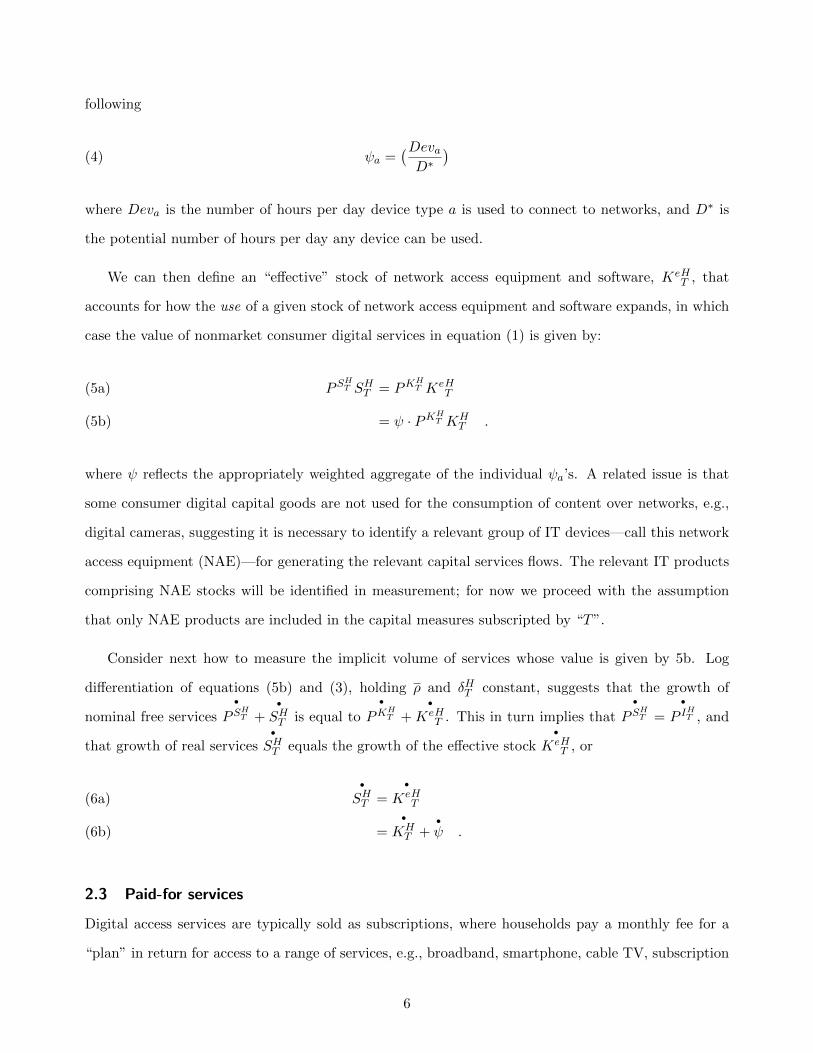
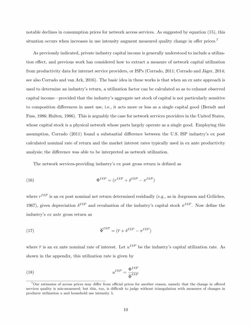
national accounts (though their paid-for predecessors often were). Consider next that the spread of

broadband since 2000 and rise of social media since 2004 suggests that the use of services that enable

the delivery of content to consumer has risen dramatically (see figure 2). The rise in use of network

services implies greater consumption volume (for a given number of subscriptions) because subscription

costs do not fully depend on use rates. All told, we translate the problem of capturing the innovations

shown in figure 1—including what Brynjolfsson and Saunders (2009) call “free goods”—into a quest

for comprehensive measurement of (a) consumer services derived from IT device use and (b) consumer

network service volumes in constant-quality terms. (a) involves an imputation to GDP for the missing

services and (b) involves creating a new price index for the paid-for services.

Because consumers’ IT capital use is inextricably tied to households’ utilization of public broad-

band, wireless, and cable networks (including their take up of over-the-top (OTT) media and personal

1The standard approach refers to the productivity literature that capitalizes consumer durables, originally due toChristensen and Jorgenson (1969, 1973); see also Jorgenson and Landefeld (2006). The U.S. national accounts do notcapitalize consumer durables in headline GDP.

Figure 1: Timeline of Innovations in Consumer Content Delivery

Source: Authors’ adaption and extension of information in Total Audience Report, The Neilsen Company, December 3, 2014,available at http://www.nielsen.com/us/en/insights/reports/2014/the-total-audience-report.html.

cloud services), its imputation must be linked to paid-for services. In other words, home services and

paid-for services exhibit demand complementarity2, and a joint analysis of these two types of consumer

digital services is required. This aspect of the approach to capitalization of consumer digital capital is

novel with this paper. A related literature addresses the measurement of “free goods” using alterna-

tive methods and very different frameworks (Nakamura, Samuels, and Soloveichik, 2016; Nakamura,

Soloveichik, and Samuels, 2018; Brynjolfsson, Collis, and Eggers, 2019; Brynjolfsson, Collis, Diewert,

Eggers, and Fox, 2019); we compare our findings to these works later in this paper.

Figure 2: Consumer Digital Capital Use

(a) Broadband Use (b) Social Media Use (c) Mobile Device Use

Source: Pew Center for the Internet

2Thanks to Shane Greenstein for suggesting this interpretation.

2

The roadmap of this paper is as follows. Section 2 sets out our framework for thinking about

how the standard framework for capitalizing consumer digital goods needs to be adjusted to take into

account the dramatic increase in household digital asset use shown in figure 2. Then we review the

relationship between device use rates and the volume of services that deliver content over networks;

this forms the basis for the quality-adjusted price index for network access services developed in this

paper, the details of which are covered in an appendix. Section 4 summarizes our empirical findings

in terms of impacts on real GDP and consumer surplus. Section 5 concludes.

Our new estimates imply that accounting for innovations in consumer content delivery matters:

The innovations boost consumer surplus by nearly $1,700 (2017 dollars) per connected user per year

for the full period of this study (1987 to 2017) and contribute more than 1/2 percentage point to

US real GDP growth during the last ten (2007 to 2017). All told, our more complete accounting

of innovations is (conservatively) estimated to have moderated the post-2007 US real GDP growth

slowdown by nearly .3 percentage point per year (out of a 1-1/2 percentage points total slowdown).

Only a portion, about .2 percentage point per year, contributes to business productivity for reasons

explained below.

2 Framework: Demand Complementarity

Digital device services and network access services work together to deliver consumer content. This

section illustrates how their demand complementarity can be exploited to capture and account for

quality change in consumer digital services.

2.1 Definitions

Because consumer digital services reflect both households’ use of digital devices and households’ take

up of network access services, the value of total consumer digital (T) services, PSTST , is expressed as

the sum of two components:

PSTST = PSHT SH

T + PSBT SB

T .(1)

The components are nonmarket (or “home”) and market (or “paid-for”) services, respectively, where

superscripts on the component digital services volume indexes (the S’s) denote location of the capital

used to deliver each type service, i.e., business sector (B) or household sector (H).

3

Home services, PSHT SH

T , are generated via households’ use of IT goods purposed for accessing digital

networks.3 Paid-for services, PSBT SB

T , are derived from subscriptions to networks, e.g., payments for

internet access, cellular access, etc. Where are the seemingly “free” services provided by Google,

Facebook and other apps? Our answer is that they are embodied in both nonmarket and market

services in this framework. The demand for consumer IT capital is a derived demand induced by the

availability of search engines, social networks (and so forth) that push users to purchase higher quality

equipment for, e.g., streaming YouTube and Netflix videos. The intensity of use of network access

services is increased because the “free” services require that data—pictures, videos, search results—

need to be delivered from the cloud for configuration and display by browsers and/or apps on the

home device. It is tempting to associate the capture of “free goods” as solved by the imputation for

home services that we propose in this paper, but the derived demand dynamic underscores it is equally

important to use quality-adjusted price statistics for the purchased parts of content delivery systems,

as improvements in quality are also seemingly “free.”

Quality change is reflected in the price indexes of both components of (1). It stems from (a) the

quality of the equipment used to access content via networks (e.g., the storage capacity of smartphones,

etc.), (b) the quality of network services (e.g., download and upload speeds of broadband service,

channel variety in video service, etc.), and (c) the use intensity of the combined content delivery system

(i.e., the equipment plus the access service). After controlling for the quality of systems (equipment

cum access services) at the time of their purchase, the change in system use intensity reflects changes

in the system’s performance, i.e., change in the marginal product of its combined net capital stocks

(just as ex post private capital income reflects changes in the return to capital). Not much of (b) and

none of (c) is in existing GDP, and while (a) is included to a significant degree, we improve its capture

in this paper.

Network use intensity reflects how consumers use their IT devices and is revealed by the take up of

paid-for network access services. Denoting network use intensity by λ, and letting N be the number

of users on the network (i.e., consumer accounts, from the perspective of the service provider), then

average network use intensity is defined as:

λ =SBT

N(2)

3IT goods used without network access produce uncounted services as well, such as personal computer used to workon local files. This use is outside the scope of our analysis.

4

where SBT is the volume of paid-for access services consumed, per equation (1). λ and N are most

easily understood from a producer perspective, i.e., λ is an intensive per customer use margin and

N is an extensive margin whose increases reflect customer growth, e.g., for broadband providers, the

number of “customers” N is households with broadband subscriptions. For cellular service providers,

N is individuals with cellular phone subscriptions.4

There are other, largely demographically-driven, dimensions of use, e.g., the number of users per

household and the age of users, as this feeds into hours of use per connection. Note that per equation (2)

these distinctions in margins of use are implicit in λ to the extent they are not counted in N .

2.2 Home services

Our starting point is the Christensen and Jorgenson (1969, 1973) framework, based on Jorgenson

(1963), for imputing service flows from capitalized consumer durables. Letting KHT denote the net

stock of digital goods held by consumers and PKHT the per period rental price for use of a unit of those

stocks, then the value of their capital services PKHT KH

T in the standard formulation would be given by:

PKHT KH

T = (ρ+ δHT )P IHT KHT(3)

where ρ is an ex ante real household discount rate, δHT is a depreciation rate for household IT stocks,

and P IHT is a quality-adjusted asset price index for new investments in those stocks.

Nominal home services for consumer digital goods, the PSHT SH

T term in equation (1), does not

correspond to equation (3) because it is essentially a capacity flow; i.e., (3) does not reflect actual, or

ex post, consumption.5 The trend in use rates illustrated in figure 2—and demand complementarity—

suggests that incorporating an “IT use” dynamic is necessary to capture the services defined by PSHT SH

T ,

i.e., there has been increased use of IT capital for consuming digital content over networks.

The IT device use dynamic is specific to each device type, which implies we need to define a use

rate ψa for each asset type a, e.g., for computers, for mobile phones, for TVs, etc. We thus have the

4Although households have other modes of network service (e.g., cable, OTT) and all such services are considered inour empirical analysis, for simplicity, the discussion in this section considers N as the number of subscriptions to a singleservice, i.e., connected households.

5Private industry capital income is generally understood to include a utilization effect when the rate of return iscalculated on an ex post basis as in Jorgenson and Griliches (1967). When consumer durables are capitalized, serviceflows are imputed using an ex ante return as in (3), and therefore a utilization effect is not be “automatically” present.See Hulten (2009) for a discussion.

5

following

ψa =(DevaD∗

)(4)

where Deva is the number of hours per day device type a is used to connect to networks, and D∗ is

the potential number of hours per day any device can be used.

We can then define an “effective” stock of network access equipment and software, KeHT , that

accounts for how the use of a given stock of network access equipment and software expands, in which

case the value of nonmarket consumer digital services in equation (1) is given by:

PSHT SH

T = PKHT KeH

T(5a)

= ψ · PKHT KH

T .(5b)

where ψ reflects the appropriately weighted aggregate of the individual ψa’s. A related issue is that

some consumer digital capital goods are not used for the consumption of content over networks, e.g.,

digital cameras, suggesting it is necessary to identify a relevant group of IT devices—call this network

access equipment (NAE)—for generating the relevant capital services flows. The relevant IT products

comprising NAE stocks will be identified in measurement; for now we proceed with the assumption

that only NAE products are included in the capital measures subscripted by “T”.

Consider next how to measure the implicit volume of services whose value is given by 5b. Log

differentiation of equations (5b) and (3), holding ρ and δHT constant, suggests that the growth of

nominal free services•

PSHT +

•

SHT is equal to

•

PKHT +

•

KeHT . This in turn implies that

•

PSHT =

•

P IHT , and

that growth of real services•

SHT equals the growth of the effective stock

•

KeHT , or

•

SHT =

•

KeHT(6a)

=•

KHT +

•ψ .(6b)

2.3 Paid-for services

Digital access services are typically sold as subscriptions, where households pay a monthly fee for a

“plan” in return for access to a range of services, e.g., broadband, smartphone, cable TV, subscription

6

video-on-demand. Each plan has a fixed set of characteristics, e.g., download speed, upload speed,

number/availability of videos or video channels, etc., for the services involved. Plan heterogeneity by

service type and service type characteristics is ignored (for now) for ease of exposition.

Producers offer digital access service plans at prices POBT . Offer prices are subscription contract

prices set at the outset of the period, and the average price each customer pays is expressed as

POB

T =POB

T OBT

N(7)

where POBT OB

T are producer revenues from consumer sales of N plans. Nominal consumer payments,

PSBT SB

T of equation (1) equals this producer sales revenue. We assume that producers’ capacity is

constrained in the short run (the period of the contract) and, after accounting for the usual issues

regarding peak load planning, that producers set offer prices based on a preferred rate of capacity

utilization determined by anticipated average customer usage, λa.

These assumptions imply that OBT is a planned quantity of delivered services and not necessarily

equal to SBT , the actual quantity of services consumed by users—unless of course actual usage λ is

perfectly anticipated, i.e., λa = λ. It follows that the offer price index POBT does not necessarily equal

the consumption price index PSBT of equation (1). Let u be an index of actual capacity utilization,

where u = 1 denotes the situation where λa = λ. We then have λ = λa u, in which case the relationship

between real services consumption and real services offered, and between consumption prices and offer

prices is given by

SBT = OB

T u.(8)

PSBT =

POBT

u.(9)

Equation (9) states that the consumption price index PSBT is a utilization-adjusted contract price.

Equations (8) and (9) are not very helpful for conventional, timely price measurement (as in

a monthly CPI) because producers’ preferred utilization rate u is not readily observed. However,

substitution of (8) into (9) reveals that the consumption price may be alternatively written as:

PSBT =

POBT OB

T

SBT

.(10)

7

which suggests that consumption prices for access services may be obtained by dividing producer

revenue by a relevant, consistently-defined volume measure, i.e., that ideally, SBT ≡ VOL where VOL is

such a measure.

What might that volume measure be? We know that total consumption increases along with

the number of users and/or hours of use, but these are very coarse indicators that do not capture

consumption intensity or service quality. An ideal measure would capture consumers’ use in terms of the

potential performance of communication networks and where utilized performance is a comprehensive

measure capable of being consistently defined in the face of rapid technical change, e.g., Internet

Protocol data traffic (IP) measured as optimally compressed megabytes/petabytes per year, i.e., that

STB ≡ VOL = IP .(11)

A range of services are delivered over networks, and dataflows/IP traffic may not always be the relevant

indicator of quality, but for internet access services via computers of mobile phones IP traffic would

appear to be a solid choice (e.g., see Abdirahman, Coyle, Heys, and Stewart, 2017). For video services,

quality is not so simple; cross-country studies have found that the quality dimension for video services is

captured by a range of controls, including the number of channels (HD and standard), and availability

of premium channels and 4K display resolution (Corrado and Ukhaneva, 2016, 2019; Dıaz-Pines and

Fanfalone, 2015).

2.4 Use intensity, λ

With real services captured by a performance measure, the changes in network and device intensity of

use,•λ, can be shown to reflect the difference between changes in the average price paid by users for a

plan and the price index for access services, i.e., it reflects changes in the quality of services consumed.

To see this, log differentiate (2):

•λ =

•

SBT −

•N .(12)

8

After adding and subtracting the nominal change in paid services,•

POBT OB

T , and combining terms, we

obtain:

•λ =

•(POBT OB

T

N

)−

•(POBT OB

T

SBT

).(13)

Substitution of (7) and (10) for the first and second terms yields:

•λ =

•

POB

T −•

PSBT .(14)

In equation (13) the change in use intensity•λ reflects the difference between the rate of change in a per

user price and a unit volume price, or per equation (14), the difference between the rate of change in

the price index for access services and rate of change in the average price per plan, i.e., quality change.

Statistical agencies generate price indexes in terms of offer prices POBT , not consumption prices

PSBT . Consider now the relationship between

•λ and the quality change in official price indexes for

network access service (based on offer prices), e.g., quality change that might be captured using hedonic

techniques that account for improvements in speeds and other capabilities in subscription telecom

service plans.6 Noting first that the change in the offer price index,•

POBT , also can be decomposed into

the rate of change in quality of offered plans,•ν, and the rate of change in the average price per plan,

•

POB

T , i.e.,•

POBT =

•

POB

T − •ν. Next, from log differentiation of (9), after subtracting the result from (14)

and combining terms, the relationship between•ν and

•λ is readily shown as

•λ =

•ν +

•u ,(15)

which says that the quality change in real network access services consumption is equal to the quality

change in offered plans (at offered prices) plus the unanticipated change in network service provider

utilization.

2.5 Network utilization, u

Consider now how one might measure u. We do not need to measure u but it helps interpret and analyze

our new price measures, e.g., it can help understand how very small increases in ν might coexist with

6As done, e.g., at the BLS (see Williams, 2008).

9

notable declines in consumption prices for network access services. As suggested by equation (15), this

situation occurs when increases in use intensity augment measured quality change in offer prices.7

As previously indicated, private industry capital income is generally understood to include a utiliza-

tion effect, and previous work has considered how to extract a measure of network capital utilization

from productivity data for internet service providers, or ISPs (Corrado, 2011; Corrado and Jager, 2014;

see also Corrado and van Ark, 2016). The basic idea in these works is that when an ex ante approach is

used to determine an industry’s return, a utilization factor can be calculated so as to exhaust observed

capital income—provided that the industry’s aggregate net stock of capital is not particularly sensitive

to composition differences in asset use, i.e., it acts more or less as a single capital good (Berndt and

Fuss, 1986; Hulten, 1986). This is arguably the case for network services providers in the United States,

whose capital stock is a physical network whose parts largely operate as a single good. Employing this

assumption, Corrado (2011) found a substantial difference between the U.S. ISP industry’s ex post

calculated nominal rate of return and the market interest rates typically used in ex ante productivity

analysis; the difference was able to be interpreted as network utilization.

The network services-providing industry’s ex post gross return is defined as

ΦISP = (rISP + δISP − πISP )(16)

where rISP is an ex post nominal net return determined residually (e.g., as in Jorgenson and Griliches,

1967), given depreciation δISP and revaluation of the industry’s capital stock πISP . Now define the

industry’s ex ante gross return as

ΦISP

= (r + δISP − πISP )(17)

where r is an ex ante nominal rate of interest. Let uISP be the industry’s capital utilization rate. As

shown in the appendix, this utilization rate is given by

(18) uISP =ΦISP

ΦISP

7Our estimates of access prices may differ from official prices for another reason, namely that the change in offeredservices quality is mis-measured; but this, too, is difficult to judge without triangulation with measures of changes inproducer utilization u and household use intensity λ.

10

which suggests that the underlying relationship between the ex post and ex ante net rate of return,

i.e., r versus r, for an industry or sector is an indicator of its capital utilization.8

2.6 Summary

To summarize, changes in the quantities and prices of consumer digital services as set out in equation (1)

are as follows:

•

SHT =

•

KHT +

•ψ(19a)

•

PSHT =

•

P IHT(19b)

•

SBT =

•V ol(19c)

•

PSBT =

•

POBT −

•λ .(19d)

where λ and ψ were defined above, and P IH

T is a quality-adjusted asset price index for network access

equipment.

3 Measurement

This section summarizes how the prices and quantities of the previous section are measured and presents

some key results; details of measurement procedures are spelled out in the appendix. We begin with

the new network access services price index, describing how this index may be built using alternative

volume measures. We then present results for•λ and for our calculations of utilization from the business

side,•u. A second subsection sets out how our consumer digital capital stocks, their connectivity use

rates, and digital capital services are obtained.

3.1 Access prices, household use intensity, and network utilization

To calculate a price index for each of the IT services provided by the business sector—cable, internet,

mobile, and video streaming—we begin with nominal spending and divide by a measure of aggregate

time spent using the service adjusted for quality. These individual price indexes are aggregated to

create an overall access price index used to deflate nominal spending on access services and produce

a measure of real spending. For exposition and analysis, we consider price indexes constructed using

8In models that introduce imperfect competition in an otherwise standard neoclassical growth framework (e.g., Rotem-berg and Woodford, 1995), utilization is absorbed in a more general inefficiency wedge capturing, among other things,the ability of firms to maintain a price markup.

11

four alternative measures of quantity: the number of households subscribed to the service, the number

of individual users, time spent on the service, and time spent adjusted for quality (our preferred

measure for deflation). Thus four alternative indexes are calculated for each of the four services by

dividing revenue by each of the alternative measures of quantity, yielding prices paid per household,

per individual, per unit of time, and per unit of constant-quality time: PSBT

H , PSBT

I , PSBT

D , and PSBT

Q .

(Note: D is the notation used for time, i.e., as in hours per Day).

The calculation of the alternative price indexes for digital access services can be summarized as

follows: Let (POBT OB

T )j be payments for service type j within total payments POBT OB

T . Price change

for each type of price index covering J types of services is then

∆lnPSBT

v =

J∑j=1

wj∆ln(POB

T OBT

VOLv

)j

where v = H, I,D,Q(20)

and wj is a Divisia payments share for digital access service type j and VOLv,j is its volume measure for

price index concept v.

Depending on the contract arrangement, the price observed by the consumer, POBT , may be any of these

four prices. For example, if a consumer pays a cable company a fixed amount to keep the household connected

each month, POBT equals P

SBT

H . If a consumer pays an internet provider a fixed amount to have unlimited access

each month, POBT equals P

SBT

I . If the consumer has a prepaid plan for a certain number of hours of talk time

on a feature phone, POBT equals P

SBT

D . And, if the consumer has a contract for smartphone use based on data

traffic consumed, POBT equals P

SBT

Q . We construct PSBT

H , PSBT

I , PSBT

D , and PSBT

Q for each service but we do not

observe POBT because we do not have information on the contract arrangements. The contract price POB

T is not

needed for the analysis in this paper; note, however, contract prices are the basis for official price measures. In

the appendix, a table documents the data sources for each access service price index and a table reports their

time series.9

In terms of the framework set out in section 2, we have the following:

∆lnPSBT = ∆lnP

SBT

Q(21)

•λ = −(∆lnP

SBT

Q − ∆lnPSBT

H )(22)

With the suite of indexes constructed along margins of use, changes in the quality-adjusted price index and in

our use intensity,•λ, which is based on households, can be decomposed into contributions from I, T , and Q—i.e.,

9Prices by access service, along with aggregate prices constructed using the alternative measures of volume, are shownin this table.

12

into contributions from growth in individuals using the service per household, time spent on the service per

individual user, and the quality of an hour of use of the service, respectively.

The aggregate quality-adjusted price index for access service corresponding to equation (21) falls 12.4 percent

per year, on average, over the full period of this study. Household use intensity,•λ, increases 13.9 percent at

an annual rate. Results for the overall price index by sub-periods are plotted in panel (a) of figure 3 below;

spending shares for its subcomponents by type are shown in panel (b) of the figure. As these figures show, the

decline in the overall quality-adjusted access price index accelerates over time, first as internet service accounts

for a rising share of spending (1997 to 2007), then as smartphone access becomes more important (2007 to 2017).

These trends in the aggregate network access price index reflect not only changes in spending shares by mode of

access but also large differences in the contributions by access mode. Decompositions for each mode of access

are shown in figure 4.

Contributions to the overall volume price change by each intensity margin (i.e, volume measure) show little

difference between changes in per individual user prices relative to per household prices; as a result, only the

contribution of changes in the price per household shows through in figure 3. As may be seen in this figure,

quality change contributes significantly to the overall decline in network access prices in most sub-periods, and

consumers’ increase in time connected provides a substantial, additional kick from 1997 to 2012. Time connected

is especially important in driving price change for spending on mobile network access and SVOD.

Figure 5 reports year-by-year changes in our overall quality-adjusted network access services price index

(PSBT

Q ) and the implied change in household use intensity (•λ) per equation (22). A price index for network access

services constructed using components of BEA’s PCE price index and our per household price index (i.e., the

average price per household, PSBT

H ) also are shown. Note first that our new access services price index (the gray

line) falls much faster than the implicit price index in existing GDP (the black line); the growth implications of

this finding will be reviewed in the next section of this paper. Note second that changes in the BEA price index

hovers about changes in our per household price from about 2000 on. If the BEA index accurately represents

changes in contract prices, the result implies that there is very little quality change in measured offer prices from

from 2000 to 2017, i.e.,•ν has shown no change since 2000.

How much of this implied zero rate of offered service quality change may be a measurement problem? It is

tempting to compare•ν with

•λ but the two are conceptually different in our framework. Using IP traffic as a

volume measure implies that•λ will reflect trends in consumer usage over and above improvements to the quality

of content delivery systems. And as previously noted, the price index based on hours per day of network use

shows the contribution of household usage rates (“time”) to our overall price index, and as illustrated in panel

(a) of figure 3, the contribution of time accounts for nearly one-half of the declines in access service prices from

1997 to 2012. The detail by type of service in figure 4 reveals that the contribution of time stems from different

13

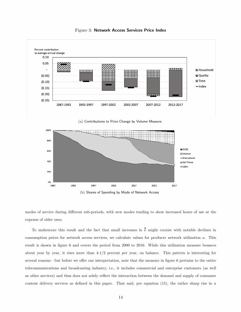
Figure 3: Network Access Services Price Index

(a) Contributions to Price Change by Volume Measure

(b) Shares of Spending by Mode of Network Access

modes of service during different sub-periods, with new modes tending to show increased hours of use at the

expense of older ones.

To underscore this result and the fact that small increases in•ν might coexist with notable declines in

consumption prices for network access services, we calculate values for producer network utilization u. This

result is shown in figure 6 and covers the period from 2000 to 2016. While this utilization measure bounces

about year by year, it rises more than 4-1/2 percent per year, on balance. This pattern is interesting for

several reasons—but before we offer our interpretation, note that the measure in figure 6 pertains to the entire

telecommunications and broadcasting industry, i.e., it includes commercial and enterprise customers (as well

as other services) and thus does not solely reflect the interaction between the demand and supply of consumer

content delivery services as defined in this paper. That said, per equation (15), the rather sharp rise in u

14

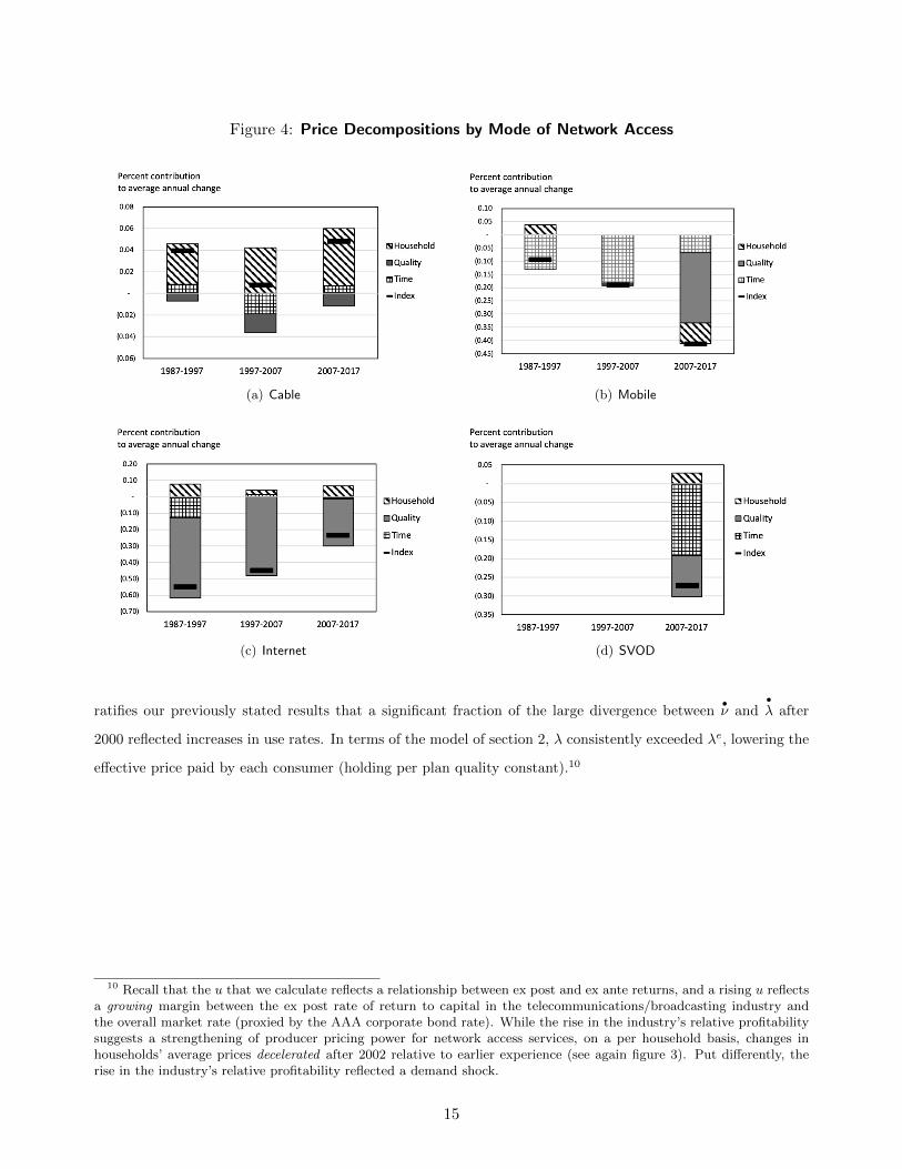
Figure 4: Price Decompositions by Mode of Network Access

(a) Cable (b) Mobile

(c) Internet (d) SVOD

ratifies our previously stated results that a significant fraction of the large divergence between•ν and

•λ after

2000 reflected increases in use rates. In terms of the model of section 2, λ consistently exceeded λe, lowering the

effective price paid by each consumer (holding per plan quality constant).10

10 Recall that the u that we calculate reflects a relationship between ex post and ex ante returns, and a rising u reflectsa growing margin between the ex post rate of return to capital in the telecommunications/broadcasting industry andthe overall market rate (proxied by the AAA corporate bond rate). While the rise in the industry’s relative profitabilitysuggests a strengthening of producer pricing power for network access services, on a per household basis, changes inhouseholds’ average prices decelerated after 2002 relative to earlier experience (see again figure 3). Put differently, therise in the industry’s relative profitability reflected a demand shock.

15

Figure 5: Consumer Network Access Services

Figure 6: Implied Network Utilization

3.2 Digital Net Stocks, Capital Services, and Asset Prices

Table 1, column (1), lists the 14 product classes of durable goods considered to be consumer durable digital

(or IT) goods. This list ranges from TVs, to computers and software, to cell phones.11 Consumer spending

for most of these products may be developed from underlying detail in the U.S. national income and product

accounts (NIPAs); indeed, the first 12 product classes shown in the table directly correspond to categories of

digital goods reported in the annual personal consumption expenditures (PCE) bridge table.12 For the analysis

in this paper, estimates of the retail value of consumer cell phone purchases are developed from industry sources;

see the appendix for further details on how this series and the other telephone equipment series are estimated.

11Game consoles, which have embodied massive innovation in the period of this study, are not included for lack of data.12BEA’s annual PCE bridge table begins in 1998 and does not extend through the most recent NIPA year. Nine

categories of PCE spending on digital goods are reported on NIPA table 2.4.5U, however, and these data are used todevelop the more detailed, bridge table-based series from 1970 to 1997 and for the year 2017.

16

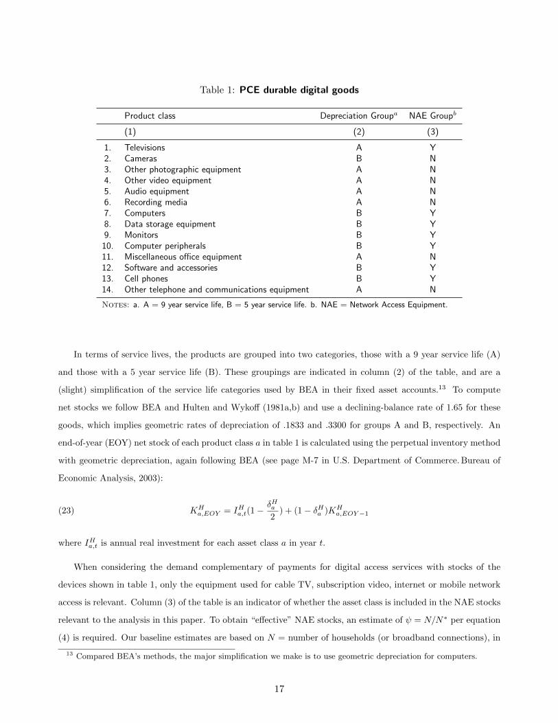
Table 1: PCE durable digital goods

Product class Depreciation Groupa NAE Groupb

(1) (2) (3)

1. Televisions A Y2. Cameras B N3. Other photographic equipment A N4. Other video equipment A N5. Audio equipment A N6. Recording media A N7. Computers B Y8. Data storage equipment B Y9. Monitors B Y

10. Computer peripherals B Y11. Miscellaneous office equipment A N12. Software and accessories B Y13. Cell phones B Y14. Other telephone and communications equipment A N

Notes: a. A = 9 year service life, B = 5 year service life. b. NAE = Network Access Equipment.

In terms of service lives, the products are grouped into two categories, those with a 9 year service life (A)

and those with a 5 year service life (B). These groupings are indicated in column (2) of the table, and are a

(slight) simplification of the service life categories used by BEA in their fixed asset accounts.13 To compute

net stocks we follow BEA and Hulten and Wykoff (1981a,b) and use a declining-balance rate of 1.65 for these

goods, which implies geometric rates of depreciation of .1833 and .3300 for groups A and B, respectively. An

end-of-year (EOY) net stock of each product class a in table 1 is calculated using the perpetual inventory method

with geometric depreciation, again following BEA (see page M-7 in U.S. Department of Commerce. Bureau of

Economic Analysis, 2003):

KHa,EOY = IHa,t(1 − δHa

2) + (1 − δHa )KH

a,EOY−1(23)

where IHa,t is annual real investment for each asset class a in year t.

When considering the demand complementary of payments for digital access services with stocks of the

devices shown in table 1, only the equipment used for cable TV, subscription video, internet or mobile network

access is relevant. Column (3) of the table is an indicator of whether the asset class is included in the NAE stocks

relevant to the analysis in this paper. To obtain “effective” NAE stocks, an estimate of ψ = N/N∗ per equation

(4) is required. Our baseline estimates are based on N = number of households (or broadband connections), in

13 Compared BEA’s methods, the major simplification we make is to use geometric depreciation for computers.

17

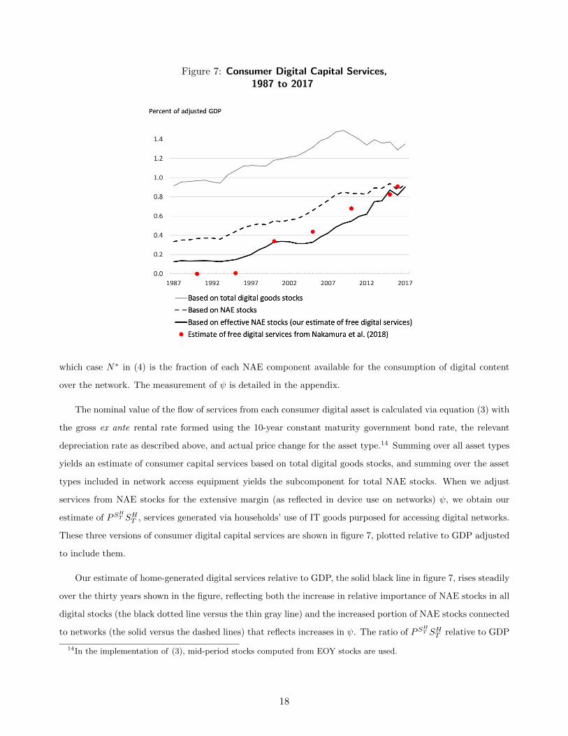
Figure 7: Consumer Digital Capital Services,1987 to 2017

which case N∗ in (4) is the fraction of each NAE component available for the consumption of digital content

over the network. The measurement of ψ is detailed in the appendix.

The nominal value of the flow of services from each consumer digital asset is calculated via equation (3) with

the gross ex ante rental rate formed using the 10-year constant maturity government bond rate, the relevant

depreciation rate as described above, and actual price change for the asset type.14 Summing over all asset types

yields an estimate of consumer capital services based on total digital goods stocks, and summing over the asset

types included in network access equipment yields the subcomponent for total NAE stocks. When we adjust

services from NAE stocks for the extensive margin (as reflected in device use on networks) ψ, we obtain our

estimate of PSHT SH

T , services generated via households’ use of IT goods purposed for accessing digital networks.

These three versions of consumer digital capital services are shown in figure 7, plotted relative to GDP adjusted

to include them.

Our estimate of home-generated digital services relative to GDP, the solid black line in figure 7, rises steadily

over the thirty years shown in the figure, reflecting both the increase in relative importance of NAE stocks in all

digital stocks (the black dotted line versus the thin gray line) and the increased portion of NAE stocks connected

to networks (the solid versus the dashed lines) that reflects increases in ψ. The ratio of PSHT SH

T relative to GDP

14In the implementation of (3), mid-period stocks computed from EOY stocks are used.

18

stood at 1.04 percent of GDP in 2017, up from .48 percent ten years earlier. This trajectory is roughly similar

to estimates of free services prepared using a very different approach (the red dots in the figure).15

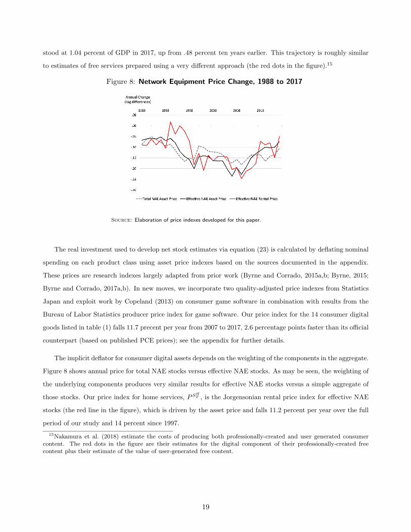
Figure 8: Network Equipment Price Change, 1988 to 2017

Source: Elaboration of price indexes developed for this paper.

The real investment used to develop net stock estimates via equation (23) is calculated by deflating nominal

spending on each product class using asset price indexes based on the sources documented in the appendix.

These prices are research indexes largely adapted from prior work (Byrne and Corrado, 2015a,b; Byrne, 2015;

Byrne and Corrado, 2017a,b). In new moves, we incorporate two quality-adjusted price indexes from Statistics

Japan and exploit work by Copeland (2013) on consumer game software in combination with results from the

Bureau of Labor Statistics producer price index for game software. Our price index for the 14 consumer digital

goods listed in table (1) falls 11.7 precent per year from 2007 to 2017, 2.6 percentage points faster than its official

counterpart (based on published PCE prices); see the appendix for further details.

The implicit deflator for consumer digital assets depends on the weighting of the components in the aggregate.

Figure 8 shows annual price for total NAE stocks versus effective NAE stocks. As may be seen, the weighting of

the underlying components produces very similar results for effective NAE stocks versus a simple aggregate of

those stocks. Our price index for home services, PSHT , is the Jorgensonian rental price index for effective NAE

stocks (the red line in the figure), which is driven by the asset price and falls 11.2 percent per year over the full

period of our study and 14 percent since 1997.

15Nakamura et al. (2018) estimate the costs of producing both professionally-created and user generated consumercontent. The red dots in the figure are their estimates for the digital component of their professionally-created freecontent plus their estimate of the value of user-generated free content.

19

4 Results and Implications

This section reports the new digital consumption measures and discusses their implications for real GDP growth

and increase in consumer surplus.

4.1 GDP

Our results for GDP are summarized in the table below. These results are calculated under the conservative

assumption that overall real GDP is unaffected by differences the PCE IT goods investment price indexes

developed in this paper and official prices used in GDP because these goods are primarily imported (whether

for “effective” investment or all IT goods spending); recall too that we are unable to include the rapid quality

change in game consoles in our price indexes.

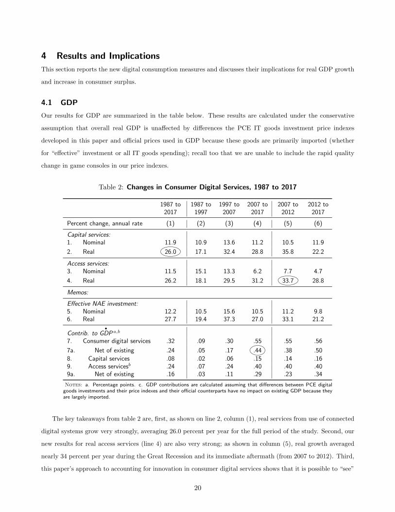
Table 2: Changes in Consumer Digital Services, 1987 to 2017

1987 to 1987 to 1997 to 2007 to 2007 to 2012 to2017 1997 2007 2017 2012 2017

Percent change, annual rate (1) (2) (3) (4) (5) (6)

Capital services:1. Nominal 11.9 10.9 13.6 11.2 10.5 11.9

2. Real 26.0 17.1 32.4 28.8 35.8 22.2

Access services:3. Nominal 11.5 15.1 13.3 6.2 7.7 4.7

4. Real 26.2 18.1 29.5 31.2 33.7 28.8

Memos:

Effective NAE investment:5. Nominal 12.2 10.5 15.6 10.5 11.2 9.86. Real 27.7 19.4 37.3 27.0 33.1 21.2

Contrib. to•

GDP a,b

7. Consumer digital services .32 .09 .30 .55 .55 .56

7a. Net of existing .24 .05 .17 .44 .38 .50

8. Capital services .08 .02 .06 .15 .14 .169. Access servicesb .24 .07 .24 .40 .40 .409a. Net of existing .16 .03 .11 .29 .23 .34

Notes: a. Percentage points. c. GDP contributions are calculated assuming that differences between PCE digitalgoods investments and their price indexes and their official counterparts have no impact on existing GDP because theyare largely imported.

The key takeaways from table 2 are, first, as shown on line 2, column (1), real services from use of connected

digital systems grow very strongly, averaging 26.0 percent per year for the full period of the study. Second, our

new results for real access services (line 4) are also very strong; as shown in column (5), real growth averaged

nearly 34 percent per year during the Great Recession and its immediate aftermath (from 2007 to 2012). Third,

this paper’s approach to accounting for innovation in consumer digital services shows that it is possible to “see”

20

digitalization in GDP. If our methods were to be incorporated in the national accounts of the United States, the

contribution of consumer digital services (both components) to real GDP growth would average .55 percentage

points from 2007 to 2017 (line 7, column 4), and annual real GDP growth would be .44 percentage points per

year higher (line 7a, column 4). These impacts are substantial.

The impacts of our work on consumer IT prices on overall PCE price measures are summarized elsewhere

Byrne and Corrado (2019); this includes the new services measures we have introduced in this paper as well as

the durable goods prices reflected on lines 5 and 6 of the table and detailed more extensively in the appendix.

With regard to changes in the trend rate of real GDP growth, the impact of using our framework for

measuring consumer digital services boosts the rate of real GDP growth from 2007 to 2017 relative to ten

years earlier (1997 to 2007) by .27 percentage point (line 7a, column 4 less column 3)—a notable acceleration.

Both the GDP boundary expansion (adding imputed real digital capital services) and the adoption of a quality-

adjusted consumption price index for network access services contribute to this acceleration, with about 60

percent stemming from the net contribution of the new access services price index (.16 percentage point). The

latter contribution also boosts business productivity growth; as with services from owner-occupied housing, the

imputation for self-generated digital capital services is not factored into conventional measures of productivity

change.

4.2 Consumer Surplus

The consumer surplus stemming from innovations in consumer content delivery can be calculated using an

index number approach if the quality-adjusted price indexes used in the analysis fully capture the benefits of

the changes in question. Assuming our price indexes are up to the task, we compute consumer surplus as the

macroececonomic gain from the relevant continuing commodities following (Diewert and Fox, 2017) as:

.5(∆ΠSH

T ∆SHT

)+ .5

(∆ΠSB

T ∆SBT

)+ .5

(∆ΠIeH

T ∆IeHT)

(24)

where ∆ is a long difference, and the ∆Π’s are changes in the relative prices, i.e.,

ΠSHT =

PSHT

PPCE, ΠSB

T =PSB

T

PPCEand ΠIeH

T =P IeH

T

PPCE,(25)

where PPCE is the overall price index for consumer spending.

In the textbook exposition of consumer surplus, the price drop from the Hicksian reservation price to the

transaction price of the new good or service is the welfare gain stemming from the innovation in question. To

fully capture this gain, benefits of individual innovations are quantified using techniques that rely on estimates

of demand elasticities or estimated parameters of utility functions in conjunction with transactions prices and

revenue data, e.g., Petrin (2002) and Greenwood and Kopecky (2013). There are many individual innovations

21

underlying our price indexes, however, and for this reason alone, eschewing a parametric approach and using (24)

has many advantages. Using (24) views innovations in digital content delivery as serial Schumpterian change

where individual innovations are launched, gain market share, and then lose market share as another innovation

is introduced. We believe this process is well captured by our quality-adjusted price indexes even though

they do not explicitly incorporate Hicksian reservation prices. Our comprehensive accounting of use intensity

captures the benefits of ubiquitous connectivity/networks cum powerful equipment in our estimates. Many of

the products that undergird these estimates experience constant change via incremental quality improvements

and introduction of new forms and varieties, and we are able to incorporate these changes, e.g., enhancements to

personal computing via new forms (tablets and cell phones) and improvements in performance (speed, storage)

are incorporated in our estimates. 16

The results of computing (24) are presented in table 3. Changes from the beginning of our sample (1987,

arguably also the beginning of the Internet) to the beginning of social media and mobile broadband (taken as

2004) are assessed, as are changes from this point to 2017, the last year of our estimates. As may be seen

on row 1, the consumer surplus due to innovations in digital content delivery from 1987 to 2004 (18 years)

was nearly $900 billion in 2017 dollars (column 1) and $4.5 trillion over the next 14 years (column 2). These

are substantial amounts. On a per user basis, rows 5 through 8, the gain hovered about $25,000 over each

period (in 2017 dollars). While these numbers seem very large (implying a per user gain in economic welfare of

nearly $1,800 per year, on average, during the latter period), they are in the same neighborhood as estimates of

consumer surplus obtained by Brynjolfsson et al. (2019) using massive online choice experiments. The sum of

their median willingness-to-pay estimates for the items included in their surveys (search engines, email, maps,

video, e-commerce, social media, messaging, and music) was $32,232 in 2017 (Brynjolfsson et al., 2019, table 7,

sum of items in column 2).

We compare our long difference estimates with the single-point-in-time survey results of Brynjolfsson et al.

(2019) based on a conjecture that respondents in their massive online experiments are thinking about what they

would have to pay to “return” to life before social media, smart phones, and mobile broadband. Brynjolfsson

et al. (2019) also report median willingness-to-pay estimates for a survey conducted in 2016, and these values

sum to $26,150, expressed in 2017 dollars.17 Using (24) with a long difference from 2004 to 2016 (i.e., dropping

16Note further that even for an innovation as significant as the iPhone, the impact of the omission of Hicksian reservationprices on a price index is very small because the revenue weight on the unobserved initial price drop is likely to be sotiny that ignoring this change has very little impact GDP or consumer surplus. As reported in Apple’s financials, totaliPhone revenue in the quarter of introduction in 2007 was $8 million ($32 million at an annual rate). GDP was $14,452billion and our digital services series was $278,334 million in that year. One half of the revenue gain from the iPhonein its introductory quarter at an annual rate was then .11×10−5 relative to GDP and .057×10−3 relative to our seriesfor connected digital capital services. Consider now the following thought experiment: Assume the change from thereservation price to the actual price of the iPhone was a ginormous -1000 percent in the quarter of introduction. Thenour price index would be off 5.7 percentage points in the initial quarter (1.4 percentage points for the year) but GDPwould be essentially unaffected.

17The simple sum of their figures is $25,697.

22

Table 3: Consumer Surplus from Innovations inContent Delivery Systems

1987 to 2004 2004 to 2017(1) (2)

Surplus, in billions of 2017 dollars:

1. Digital goods and services, total 879 4,4502. Capital investment 257 7883. Capital services 303 1,4094. Access services 319 2,254

Surplus, in thousands of $ per usera:

5. Digital goods and services, total 26,926 23,0816. Capital investment 7,855 4,0877. Capital services 9,292 7,0368. Access services 9,779 11,689

Annual surplus per user:

9. Digital goods and services, total 1,548 1,77510. Capital investment 462 31411. Capital services 547 56212. Access services 575 889

Note: All figures are in 2017 dollars.a. The per user figure is obtained by dividing the results on rows 1 to 4 by the averagenumber of connected users during the period indicated.

the last year, and dividing by a slightly lower number for the average number of users) yields an estimate of the

consumer surplus of $19,502 per user—again in the same ballpark and, we believe, strengthening our conjecture.

5 Conclusion

The household is an important locus of the digital revolution and one of its most visible since smartphones and

social media became widespread. Entertainment, communication, and work from home have been supercharged

by advances in hardware, software, and communication. Hardware innovation has proceeded at an especially

blistering pace as the major household platforms—smartphones, tablets, televisions, gaming consoles and all the

apps that run on them—have become extraordinarily powerful (and cheap) and as datacenter innovation (i.e. the

cloud) has charged ahead in the background. Faster communication speeds—both wireline and wireless—have

been essential of course; for example, nearly one-third of all IP traffic in 2016 was accounted for by Netflix alone,

a usage volume not possible one or two years earlier.

The highly visible innovations in consumer content delivery raises the question of whether existing national

accounts are missing consequential growth in output and income associated with content delivered to consumers

via their use of digital platforms. The changing production border for digital content delivery suggests that GDP

(as well as other macroeconomic measures, such as PCE prices) need to account for the substitution away from

market-based digital services consumption. While substitution between market activity and household activity

23

has long been an issue in national accounting, arguably it does not typically surface as a first-order measurement

issue beyond the case of owner-occupied housing, which is addressed in the accounts.18

We believe the digitization of consumer content delivery presents a case akin to the selective treatment of

housing in national accounts and that an imputation for omitted services for connected IT capital needs to be

made to avoid imparting a bias to GDP. The case for imputation of owner-occupied housing is based on the

size of the omitted services and the importance of accounting for it in international comparisions. The case we

offer for accounting for the digitization of consumer content via an imputation for connected IT capital services

is based on the relatively fast growth of the omitted services, i.e., the case rests on the fact that the omitted

services provide an extra kick to real GDP due to their declining relative price (i.e., like business IT investment

and service prices, as set out in Byrne and Corrado, 2017b). To restate the empirical relevance of the case, we

estimate that consumer welfare due to growth in digital content consumption has been enhanced to the tune of

$1,775 per connected user per year from 2004 to 2017 (2017 dollars). And when our demand complementarity

framework is incorporated into existing GDP, we find that real consumer digital services contributes nearly

.6 percentage points per year to U.S. economic growth from 2007 to 2017.

18Food produced and consumed on farms is another example of an imputation long included in national accounts toaddress substitution between home-produced and market activity, but it is not large in advanced economies.

24

ReferencesAbdirahman, M., D. Coyle, R. Heys, and W. Stewart (2017). A comparison of approaches to deflating telecoms

services output. Technical Report Discussion Paper 2017-04, ESCoE and ONS.

Aizcorbe, A., D. M. Byrne, and D. E. Sichel (2019). Getting smart about phones: New price indexes and theallocation of spending between devices and services plans in personal consumption expenditures. WorkingPaper No. 25645, National Bureau of Economic Research.

Berndt, E. R. and M. A. Fuss (1986). Productivity measurement with adjustments for variations in capacityutilization and other forms of temporary equilibrium. Journal of Econometrics 33 (1), 7–29.

Brynjolfsson, E., A. Collis, W. E. Diewert, F. Eggers, and K. J. Fox (2019). GDP-B: Accounting for the value ofnew and free goods in the digital economy. Working Paper No. 25695 (March), National Bureau of EconomicResearch.

Brynjolfsson, E., A. Collis, and F. Eggers (2019). Using massive online choice experiments to measure changesin well-being. Proceedings of the National Academy of Sciences 116 (15), 7250–7255.

Brynjolfsson, E. and A. Saunders (2009). Wired for innovation: How information technology is reshaping theeconomy. MIT Press.

Byrne, D. M. (2015). Prices for data storage equipment and the state of IT innovation. FEDS Notes (July 15),Federal Reserve Board, Washington, D.C.

Byrne, D. M. and C. A. Corrado (2015a). Prices for communications equipment: Rewriting the record. Financeand Economics Discussion Series 2015-069 (September), Board of Governors of the Federal Reserve System,Washington, D.C.

Byrne, D. M. and C. A. Corrado (2015b). Recent trends in communications equipment prices. FEDS Notes(September 29), Federal Reserve Board, Washington, D.C.

Byrne, D. M. and C. A. Corrado (2017a). ICT asset prices: Marshalling evidence into new measures. Financeand Economics Discussion Series 2017-016 (February), Board of Governors of the Federal Reserve System,Washington.

Byrne, D. M. and C. A. Corrado (2017b). ICT Services and their Prices: What do they tell us about Productivityand Technology? International Productivity Monitor (33), 150–181.

Byrne, D. M. and C. A. Corrado (2019). Consumer price misstatement: IT prices in the 21st century. Technicalreport, (forthcoming).

Christensen, L. R. and D. W. Jorgenson (1969). The measurement of US real capital input, 1929–1967. Reviewof Income and Wealth 15 (4), 293–320.

Christensen, L. R. and D. W. Jorgenson (1973). Measuring economic performance in the private sector. InM. Moss (Ed.), The Measurement of Economic and Social Performance, pp. 233–351. NBER.

Copeland, A. (2013). Seasonality, consumer heterogeneity and price indexes: the case of prepackaged software.Journal of Productivity Analysis 39, 47–59.

Corrado, C. (2011). Communication capital, Metcalfe’s law, and U.S. productivity growth. Economics ProgramWorking Paper 11-01, The Conference Board, Inc., New York. Available at http://papers.ssrn.com/sol3/papers.cfm?abstract_id=2117784.

Corrado, C. and K. Jager (2014). Communication networks, ICT, and productivity growth in Europe. EconomicsProgram Working Paper 14-04, The Conference Board, Inc., New York.

Corrado, C. and O. Ukhaneva (2016). Hedonic Prices for Fixed Broadband Services: Estimation across OECDCountries. Technical report, OECD/STI Working Paper.

25

Corrado, C. and O. Ukhaneva (2019). Hedonic Price Measures for Fixed Broadband Services: Estimation acrossOECD Countries, Phase II. Technical report, OECD/DSTI/CDEP Report to CISP and MADE, revised.

Corrado, C. A. and B. van Ark (2016). The Internet and productivity. In J. M. Bauer and M. Latzer (Eds.),Handbook on the Economics of the Internet, pp. 120–145. Northamption, Mass.: Edward Elgar Publishing,Inc.

Dıaz-Pines, A. and A. G. Fanfalone (2015). The role of triple- and quadruple-play bundles: Hedonic priceanalysis and industry performance in France, the United Kingdom, and the United States. Paper presentedat 43rd research conference on commmunications, information and internet policy, George Mason UniversitySchool of Law, Arlington, VA.

Diewert, W. E. and K. Fox (2017). The digital economy, GDP and consumer welfare, paper presented at theCRIW workshop, NBER Summer Institute, Cambridge MA (July 17–18).

Gordon, R. J. (1990). The Measurement of Durable Goods Prices. Chicago: University of Chicago Press.

Greenwood, J. and K. A. Kopecky (2013). Measuring the welfare gain from personal computers. EconomicInquiry 51 (1), 336–347.

Hulten, C. (1986). Productivity change, capacity utilization, and the sources of efficiency growth. Journal ofEconometrics 33, 31–50.

Hulten, C. (2009). Growth accounting. Working paper, NBER Working Paper 15341 (September).

Hulten, C. R. and F. C. Wykoff (1981a). The estimation of economic depreciation using vintage asset prices.Journal of Econometrics 15, 367–396.

Hulten, C. R. and F. C. Wykoff (1981b). The measurement of economic depreciation. In C. R. Hulten (Ed.),Depreciation, Inflation & the Taxation of Income from Capital, pp. 81–125. The Urban Institute.

Jorgenson, D. W. (1963). Capital theory and investment behavior. American Economic Review 53 (2), 247–259.

Jorgenson, D. W. and Z. Griliches (1967). The explanation of productivity change. The Review of EconomicStudies 34 (3), 249–283.

Jorgenson, D. W. and J. S. Landefeld (2006). Blueprint for expanded and integrated U.S. accounts: Review,assessment, and next steps. In D. W. Jorgenson, J. S. Landefeld, and W. D. Nordhaus (Eds.), A NewArchitecture for the U.S. National Accounts, Volume 66 of NBER Studies in Income and Wealth, pp. 13–112.Chicago: University of Chicago Press. Available at http://www.nber.org/chapters/c0133.pdf.

Nakamura, L., J. Samuels, and R. Soloveichik (2016). Valuing ‘free’ media in GDP: An experminental approach.Technical report, Bureau of Economic Analysis.

Nakamura, L., R. Soloveichik, and J. Samuels (2018). “Free” Internet Content: Web 1.0, Web 2.0, and the sourcesof economic growth. Technical Report Research Paper WP 18-17, Federal Reserve Bank of Philadelphia.

Petrin, A. (2002). Quantifying the benefits of new products: The case of the minivan. Journal of PoliticalEconomy 110 (4), 705–729.

Rotemberg, J. J. and M. Woodford (1995). Dynamic general equilibrium models with imperfectly competitiveproduct markets. In T. F. Cooley (Ed.), Frontiers of Business Cycle Research, pp. 243–293. PrincetonUniversity Press.

U.S. Department of Commerce. Bureau of Economic Analysis (2003). Fixed Assets and Consumer DurablesGoods in the United States, 1925–99. Washington, D.C.: U.S. Government Printing Office.

Williams, B. (2008). A hedonic model for Internet access service in the Consumer Price Index. Monthly LaborReview (July), 33–48.

26

Appendixes

A1 Network utilizationThis appendix provides a derivation of equation (18) in the main text, i.e., we set out how to extract a measureof network capital utilization from productivity data and documents the calculations reported in section 3.1.

A1.1 DerivationWhat follows is based on the framework set out for analyzing communication networks and network externalitiesin Corrado (2011), in which it is assumed there no markups due to imperfect competition or other inefficiencywedges; see also Corrado and Jager (2014) and Corrado and van Ark (2016).

In sources-of-growth accounting, the contribution of private capital is expressed in terms of the services itprovides. Let the value of the relevant private stocks be denoted as P IK where the price of each unit of capitalP I is the investment price and the real stock K is a quantity obtained via the standard perpetual inventorymodel. In our application, the value P IK represents the replacement value of network service provider capital interms of its capacity to deliver digital services (i.e., including in this application, the value of the “originals” forthe content the provider can diseminate). The value PKK represents the service flow provided by that capital.

The price PK is an unobserved rental equivalence price, but which is related to the investment price by theuser cost formula, PK = P I(r + δ − π)T , where r is an after-tax ex post rate of return, δ the depreciation rateused in the perpetual inventory calculation, π is capital gains, and T is the Hall-Jorgenson tax term. The rentalequivalence price is simplified by defining the gross return Φ = (r+ δ−π)T , so that when capital services PKKare equated with observed capital income via the residual calculation of an ex post after-tax rate of return r, wehave

(A1) observed capital income = P IK ∗ Φ

When capital services are computed on the basis of an ex ante financial rate of return r, the value for capitalincome of network providers must be expressed differently. Defining the ex ante gross return Φ = (r + δ − π)Taccordingly, network provider capital income is expressed as

(A2) observed capital income = P IKuISP ∗ Φ

where uISP is network capital utilization and, via Berndt and Fuss (1986), capital utilization uISP (rather thanr) exhausts capital income.

Equating expressions (A1) and (A2)

P IK ∗ Φ = P IKuISP ∗ Φ

and solving for uISP yields

(A3) uISP =Φ

Φ.

This equation states that under the conditions set out in Berndt and Fuss (1986) the relationship between theex post and ex ante gross rate of return for an industry or sector reflects its capital utilization.

A1.2 CalculationsThe implied network utilization calculating according to equation (A3) where r in the definition of Φ is calculatedfollowing Jorgenson and Griliches (1967) as the ex post return for the combined Motion Picture, Sound Recording,Telecommunications, and Broadcasting industries (NAICS 512,515,517) and where r in the definition of Φ is setto Moody’s AAA corporate bond rate.

The ex post net return and the δ and π components of Φ and Φ were calculated by the authors for thecombined sector using data from BEA’s industry accounts (accessed October 2018). The results for u are shownin text figure 6.

27

A2 Access Service Prices and ConsumptionTo calculate a price index for each of the network access services provided by the business sector—cable, internet,mobile, and subscriptionvideo streaming—we begin with nominal spending and divide by a measure of aggregatetime spent using the service adjusted for quality. These individual price indexes are aggregated to createan overall access price index used to deflate nominal spending on access services and produce a measure ofconsumption.

For exposition and analysis, we also consider price indexes constructed using four alternative measures ofquantity: the number of households subscribed to the service, the number of individual users, time spent on theservice, and time spent adjusted for quality (our preferred measure for deflation). Thus four alternative indexesare calculated for each of the four services by dividing revenue by each of the alternative measures of quantity,yielding prices paid per household, per individual, per unit of time, and per unit of constant-quality time: PH ,PI , PD, and PQ.

Data sources and calculation methods for service prices are summarized in 9.

A2.1 Nominal SpendingFor nominal spending, we use figures from the national accounts published by Bureau of Economic Analysis,table 2.4.5U, “Personal Consumption Expenditures by Type of Product.” In the cases of mobile access andvideo on demand, we developed additional detail as explained below.

Cable Spending is taken from table line 215, “Cable, satellite, and other live television services.” We use“cable” as shorthand for spending in this category, which includes spending on the services of multi-channelvideo programming distributors (MVPDs) of all kinds, including in addition to cable television, programmingprovided via telecommunications service provider, direct broadcast satellite, home satellite dish, wireless cable,master antenna, and open video systems.

Internet Spending is taken from table line 285, “Internet access.” Spending on internet services includesaccess via “dial-up” service and access via broadband whether obtained through a telecommunications serviceprovider, a cable system, or a satellite system. We extrapolate a spending figure for 1987 using the growth rateof internet households.

Mobile Spending is taken from table line 281, “Cellular telephone services.” Mobile services spending includesaccess to broadband via smartphone as well as access to conventional features such as voice and text usingsmartphone or feature phone. We split nominal access spending between smartphone service and feature phoneservice, for which we construct distinct quantity measures, using the number of subscribers of each type (derivedas explained below) and a judgmental assumption that price paid for a smartphone contract is four times theprice paid for a feature phone contract. (At the time of writing, a casual review of prices on the WorldwideWeb showed basic plans with no data were $10-15 per month and common smartphone plans were $40-60 permonth.)

Video Total video spending is taken from table line 220, “Video streaming and rental.”19 We focus onsubscription video on demand (SVOD), which we use as an indicator for the broader category, due to datalimitations.20 In particular, we construct estimates of revenue for the three most prominent SVOD providers–Netflix, Amazon Prime, and Hulu—based on company financial reports and press reports. Netflix reports revenueper subscription beginning in 2012, which we extrapolate back to 2007 using the modest 2012-2013 growth rate.Revenue per subscription for Amazon and Hulu are assumed to be their standard charges ($7.99 per month forHulu and $79 per year for Amazon Prime through 2013 and $99 per year afterward). These figures are multipliedby the number of households for each service estimated as described below.

19BEA also provides revenue for “Audio streaming and radio services (including satellite radio)”. We did not developa price index for this category.

20In addition to SVOD, video streaming and rental as defined in the NIPAs encompasses one-off video on demand,such as sports events, and rental of DVDs, for which we do not have data.

28

A2.2 HouseholdsCable Periodic reports from the FCC, “Status of Competition in Markets for the Delivery of Video Program-ming,” provide household subscription figures for 1990 to 2015, citing reports by consulting firm SNL Kagan.Earlier years were collected from Statistical Abstracts of the United States, which reports figures from Census ofHousing. Figures for 2016 and 2017 were extrapolated using available reports from cable, telecom, and satelliteservice companies (Chartered, Comcast, AT&T, Verizon, DIRECTV, and DISH).

Internet Periodic reports from the FCC, “Internet Access Services: Status,” provide household figures forbroadband access for 1999-2016 and dial-up access for 2001-2009. Prior to 1999, we assume all access wasvia dial-up service. Dial-up service figures for years not covered by FCC reports were available from financialreports and press reports for America Online, Compuserve, Prodigy, Microsoft Network, AT&T Worldnet, andGenie. The company series were judgmentally extrapolated to the year of introduction for each service. Dial-upsubscribers from 2010 onward were extrapolated using figures from America Online (AOL) through 2014 andthe 2011-2014 rate of AOL subscription decline for 2015-2017.

Mobile We do not have data on the number of households with cell phone service. We assume the share ofhouseholds with service equals the share of individuals in the adult population with service.

Video Netflix reports the number of paying members beginning in 2009, which we extrapolate back to 2007using the 2009-2010 growth rate. Hulu and Amazon subscribers are collected from press reports, which typi-cally cite estimates from eMarketer. Because eMarketer figures estimate the number of active users using anassumption of 2.5 users per subscribing household, we multiply these reported user figures by 0.4 to estimatethe number of households, assuming one subscription per household.

A2.3 IndividualsCable We scale cable household figures using the number of residents at least two years of age per TV householdreported by Nielsen for 1985, 1990, 1995, 2000, 2005, and 2010, interpolated and extrapolated.

Internet In 1998, 2000, 2001, 2003, 2007, 2009-2013, 2015, and 2017, the Current Population Survey supple-mental survey on computer and internet use provided estimates of the share of people living in a household withan internet connection and the share of individuals going online at home. We use this information to construct atime series for the share of people who use the internet at home for 1998-2017 for adults and children separately.We extrapolate these shares back to 1987 using the growth rate for 1998-2009. These shares are applied to theaverage composition by age of U.S. households to derive the total number of home internet users by year.

Mobile Number of cellphone users (smartphone and feature phone collectively) is taken from ConsumerTelecommunications Industry Association (CTIA) estimates as reported in Statistical Abstracts of the UnitedStates for 1987-2004. Estimates for 2005-2017 are from population shares reported by the Pew Research Cen-ter (Pew) times the U.S. population. Pew also provides separate estimates for smartphone users, which aresubtracted from total cellphone users to get (solely) feature phone users.

Video For each SVOD service, the number of users is estimated by multiplying the number of householdstimes the average household size reported by the U.S. Census for the year. That is, we assume all householdmembers make use of the service.

A2.4 Time UseCable The Nielsen Corporation (Nielsen) provides time spent per day on live and time-shifted television byage group (2-11 years old, 12-17 years old, at least 18 years old) beginning in 1992, which we extrapolate to1987 using the value for 1992. We weight these figures by the U.S. Census-reported share of the population atleast 2 years old for each age group to get an average hours per day for residents of households with cable accesswhich we multiply by total users to get total hours.

29

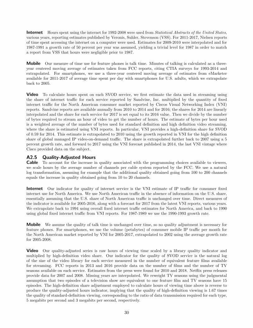
Internet Hours spent using the internet for 1992-2008 were used from Statistical Abstracts of the United States,various years, reporting estimates published by Veronis, Suhler, Stevenson (VSS). For 2011-2017, Nielsen reportsof time spent accessing the internet on a computer were used. Estimates for 2009-2010 were interpolated and for1987-1991 a growth rate of 50 percent per year was assumed, yielding a trivial level for 1987 in order to matcha report from VSS that hours were negligible prior to 1987.

Mobile Our measure of time use for feature phones is talk time. Minutes of talking is calculated as a three-year centered moving average of estimates taken from FCC reports, citing CTIA surveys for 1993-2014 andextrapolated. For smartphones, we use a three-year centered moving average of estimates from eMarketeravailable for 2011-2017 of average time spent per day with smartphones for U.S. adults, which we extrapolateback to 2005.

Video To calculate hours spent on each SVOD service, we first estimate the data used in streaming usingthe share of internet traffic for each service reported by Sandvine, Inc. multiplied by the quantity of fixedinternet traffic for the North American consumer market reported by Ciscos Visual Networking Index (VNI)reports. Sandvine reports are available annually from 2010 to 2014 and for 2016; the shares for 2014 are linearlyinterpolated and the share for each service for 2017 is set equal to its 2016 value. Then we divide by the numberof bytes required to stream an hour of video to get the number of hours. The estimate of bytes per hour usedis a weighted average of the number of bytes used for standard definition and high definition video streaming,where the share is estimated using VNI reports. In particular, VNI provides a high-definition share for SVODof 0.59 for 2014. This estimate is extrapolated to 2010 using the growth reported in VNI for the high definitionshare of global managed IP video-on-demand traffic. The share is extrapolated further back to 2007 using a 5percent growth rate, and forward to 2017 using the VNI forecast published in 2014, the last VNI vintage whereCisco provided data on the subject.

A2.5 Quality-Adjusted HoursCable To account for the increase in quality associated with the programming choices available to viewers,we scale hours by the average number of channels per cable system reported by the FCC. We use a naturallog transformation, assuming for example that the additional quality obtained going from 100 to 200 channelsequals the increase in quality obtained going from 10 to 20 channels.

Internet Our indicator for quality of internet service is the VNI estimate of IP traffic for consumer fixedinternet use for North America. We use North American traffic in the absence of information on the U.S. share,essentially assuming that the U.S. share of North American traffic is unchanged over time. Direct measures ofthe indicator is available for 2005-2016, along with a forecast for 2017 from the latest VNI reports, various years.We extrapolate back to 1994 using overall fixed internet traffic estimates for North America, and back to 1990using global fixed internet traffic from VNI reports. For 1987-1989 we use the 1990-1993 growth rate.

Mobile We assume the quality of talk time is unchanged over time, so no quality adjustment is necessary forfeature phones. For smartphones, we use the volume (petabytes) of consumer mobile IP traffic per month forthe North American market reported by VNI for 2005-2017, extrapolated to 2002 using the average growth ratefor 2005-2008.

Video Our quality-adjusted series is raw hours of viewing time scaled by a library quality indicator andmultiplied by high-definition video share. Our indicator for the quality of SVOD service is the natural logof the size of the video library for each service measured in the number of equivalent feature films availablefor streaming. FCC reports in 2013 and 2016 provide data on the number of films and the number of TVseasons available on each service. Estimates from the press were found for 2010 and 2018. Netflix press releasesprovide data for 2007 and 2008. Missing years are interpolated. We reweight TV seasons using the judgmentalassumption that two episodes of a television show are equivalent to one feature film and TV seasons have 15episodes. The high-definition share adjustment employed to calculate hours of viewing time above is reverse toproduce the quality-adjusted hours indicator, implying that the quality of high-definition viewing is 1.67 timesthe quality of standard-definition viewing, corresponding to the ratio of data transmission required for each type,5 megabits per second and 3 megabits per second, respectively.

30

A2.5.1 Price Indexes

Table 13 shows the quality-adjusted price index for each access service and price indexes for each concept ofquantity. Our aggregate quality-adjusted price index for access service, shown in the right-most column, falls12.4 percent per year, on average, over the full period of this study. The price index decline accelerates overtime, first as internet service accounts for a rising share of spending, in the 1997-2007 period, then as mobile andvideo on demand access become more important in the 2007-2017 period. (Decomposition of of growth rates inthe final index into contributions from each margin is discussed in the paper.)

31

Fig

ure

9:S

ourc

esan

dM

eth

od

sfo

rA

cces

sS

ervic

eP

rice

s

(a)Cab

lean

dInternet

32

Fig

ure

9:S

ourc

esan

dM

eth

od

sfo

rA

cces

sS

ervic

eP

rice

s

(b)Feature

Phonean

dSmartphone

33

Fig

ure

9:S

ourc

esan

dM

eth

od

sfo

rA

cces

sS

ervic

eP

rice

s

(c)SubscriptionVideo

onDem

and

34

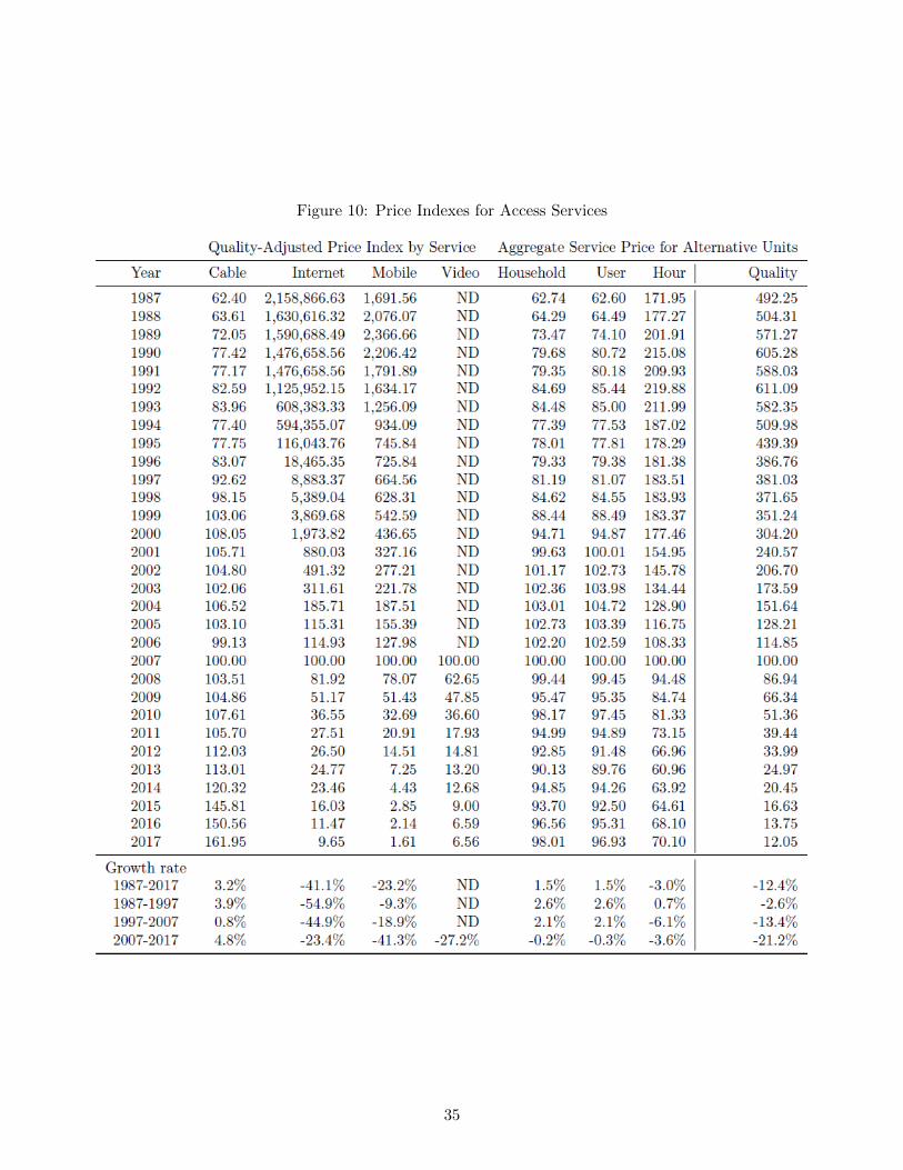
Figure 10: Price Indexes for Access Services

35

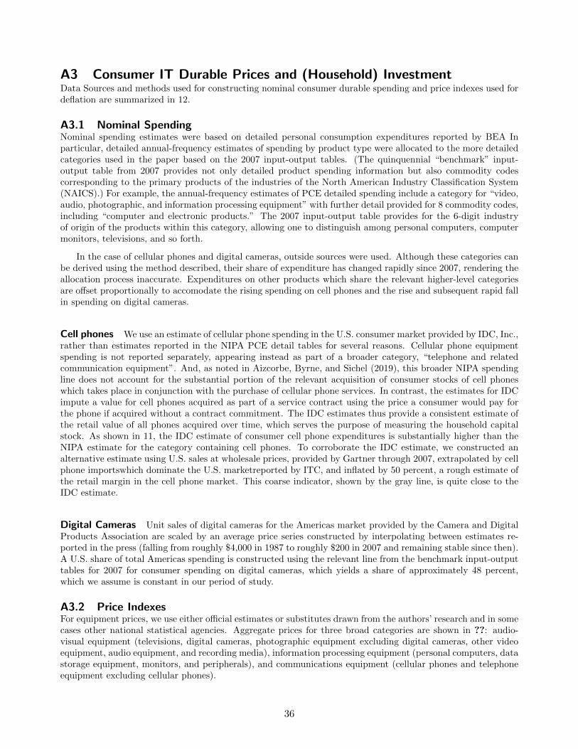
A3 Consumer IT Durable Prices and (Household) InvestmentData Sources and methods used for constructing nominal consumer durable spending and price indexes used fordeflation are summarized in 12.

A3.1 Nominal SpendingNominal spending estimates were based on detailed personal consumption expenditures reported by BEA Inparticular, detailed annual-frequency estimates of spending by product type were allocated to the more detailedcategories used in the paper based on the 2007 input-output tables. (The quinquennial “benchmark” input-output table from 2007 provides not only detailed product spending information but also commodity codescorresponding to the primary products of the industries of the North American Industry Classification System(NAICS).) For example, the annual-frequency estimates of PCE detailed spending include a category for “video,audio, photographic, and information processing equipment” with further detail provided for 8 commodity codes,including “computer and electronic products.” The 2007 input-output table provides for the 6-digit industryof origin of the products within this category, allowing one to distinguish among personal computers, computermonitors, televisions, and so forth.

In the case of cellular phones and digital cameras, outside sources were used. Although these categories canbe derived using the method described, their share of expenditure has changed rapidly since 2007, rendering theallocation process inaccurate. Expenditures on other products which share the relevant higher-level categoriesare offset proportionally to accomodate the rising spending on cell phones and the rise and subsequent rapid fallin spending on digital cameras.

Cell phones We use an estimate of cellular phone spending in the U.S. consumer market provided by IDC, Inc.,rather than estimates reported in the NIPA PCE detail tables for several reasons. Cellular phone equipmentspending is not reported separately, appearing instead as part of a broader category, “telephone and relatedcommunication equipment”. And, as noted in Aizcorbe, Byrne, and Sichel (2019), this broader NIPA spendingline does not account for the substantial portion of the relevant acquisition of consumer stocks of cell phoneswhich takes place in conjunction with the purchase of cellular phone services. In contrast, the estimates for IDCimpute a value for cell phones acquired as part of a service contract using the price a consumer would pay forthe phone if acquired without a contract commitment. The IDC estimates thus provide a consistent estimate ofthe retail value of all phones acquired over time, which serves the purpose of measuring the household capitalstock. As shown in 11, the IDC estimate of consumer cell phone expenditures is substantially higher than theNIPA estimate for the category containing cell phones. To corroborate the IDC estimate, we constructed analternative estimate using U.S. sales at wholesale prices, provided by Gartner through 2007, extrapolated by cellphone importswhich dominate the U.S. marketreported by ITC, and inflated by 50 percent, a rough estimate ofthe retail margin in the cell phone market. This coarse indicator, shown by the gray line, is quite close to theIDC estimate.

Digital Cameras Unit sales of digital cameras for the Americas market provided by the Camera and DigitalProducts Association are scaled by an average price series constructed by interpolating between estimates re-ported in the press (falling from roughly $4,000 in 1987 to roughly $200 in 2007 and remaining stable since then).A U.S. share of total Americas spending is constructed using the relevant line from the benchmark input-outputtables for 2007 for consumer spending on digital cameras, which yields a share of approximately 48 percent,which we assume is constant in our period of study.

A3.2 Price IndexesFor equipment prices, we use either official estimates or substitutes drawn from the authors’ research and in somecases other national statistical agencies. Aggregate prices for three broad categories are shown in ??: audio-visual equipment (televisions, digital cameras, photographic equipment excluding digital cameras, other videoequipment, audio equipment, and recording media), information processing equipment (personal computers, datastorage equipment, monitors, and peripherals), and communications equipment (cellular phones and telephoneequipment excluding cellular phones).

36

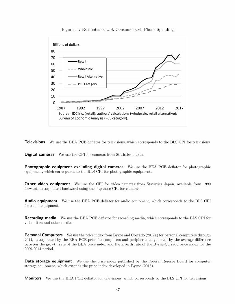
Figure 11: Estimates of U.S. Consumer Cell Phone Spending

0

10

20

30

40

50

60

70

80

1987 1992 1997 2002 2007 2012 2017

Retail

Wholesale

Retail Alternative

PCE Category

Billions of dollars

Source.  IDC Inc. (retail); authors' calculations (wholesale, retail alternative);Bureau of Economic Analysis (PCE category).

Televisions We use the BEA PCE deflator for televisions, which corresponds to the BLS CPI for televisions.

Digital cameras We use the CPI for cameras from Statistics Japan.

Photographic equipment excluding digital cameras We use the BEA PCE deflator for photographicequipment, which corresponds to the BLS CPI for photographic equipment.

Other video equipment We use the CPI for video cameras from Statistics Japan, available from 1990forward, extrapolated backward using the Japanese CPI for cameras.

Audio equipment We use the BEA PCE deflator for audio equipment, which corresponds to the BLS CPIfor audio equipment.

Recording media We use the BEA PCE deflator for recording media, which corresponds to the BLS CPI forvideo discs and other media.

Personal Computers We use the price index from Byrne and Corrado (2017a) for personal computers through2014, extrapolated by the BEA PCE price for computers and peripherals augmented by the average differencebetween the growth rate of the BEA price index and the growth rate of the Byrne-Corrado price index for the2009-2014 period.

Data storage equipment We use the price index published by the Federal Reserve Board for computerstorage equipment, which extends the price index developed in Byrne (2015).

Monitors We use the BEA PCE deflator for televisions, which corresponds to the BLS CPI for televisions.

37

Computer peripherals We use the price index from Byrne and Corrado (2017a) for peripherals through2014, extrapolated by the BEA PCE price for computers and peripherals augmented by the average differencebetween the growth rate of the BEA price index and the growth rate of the Byrne-Corrado price index for the2009-2014 period.

Other information processing equipment We use the BEA PCE deflator for calculators, typewriters, andother information processing equipment.

Software and accessories We use the price index for prepackaged software from Byrne and Corrado (2017a)for non-game PCE software, extrapolated for 2015-2017 using the 5-year average growth rate. For gaming PCEsoftware, we use the BLS producer price index for game software publishing, available for 1998-2009 and 2014-2017, adjusted for the average difference between the PPI and Copeland (2013) over the 1998-2004 period. The2010-2013 period is interpolated using the average growth rate in our index for the 2005-2009 period. For the1987-1997 period, we use the BEA PCE price index for computer software and accessories.

Cell phones We use the Byrne and Corrado (2015a) price index for cell phones for the 1987-2010 period andthe Aizcorbe et al. (2019) index for 2010-2017.

Telephone equipment excluding cellular phones We use the Byrne and Corrado (2017a) price index fortelephones for the 1987-2014 period as extended and published by the Federal Reserve Board through 2017.

38

Fig

ure

12:

Sou

rces

and

Met

hod

sfo

rC

onsu

mer

Cap

ital

Sp

end

ing

and

Pri

ces

(a)Audio-V

isual

andCommunicationsEquipment

39

Fig

ure

12:

Sou

rces

and

Met

hod

sfo

rC

onsu

mer

Cap

ital

Sp

end

ing

and

Pri

ces

(b)Inform

ationProcessingEquipment

40

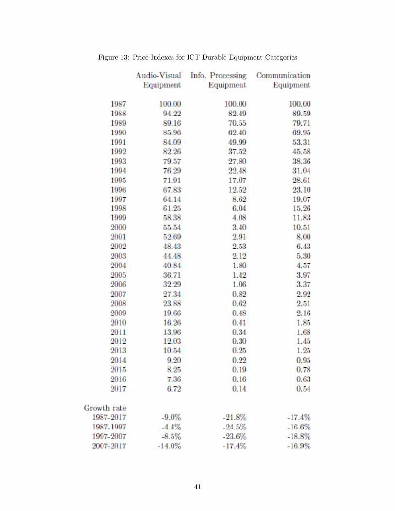
Figure 13: Price Indexes for ICT Durable Equipment Categories

41

A4 IT Durable Use Intensity, Service Prices and ConsumptionWe construct measures of use intensity for each type of capital employed to connect to the access servicesdiscussed in the paper. These include personal computers and related capital (monitors, software, and datastorage equipment), televisions, and cell phones. These use intensity measures allow us to identify the effect onIT capital services from users spending a greater share of their time on digital access services and consequentlythe imprint that free and purchased services have on consumption.

Mechanically, constructing use intensity for a particular type of capital requires allocating time spent onaccessing each digital service to the capital used for the access. For example, use intensity for personal computersis proportional to the share of household time spent accessing fixed internet services plus the portion of time spentusing SVOD when viewing programming through the computer. Likewise, television use intensity is affected bycable access and by a portion of SVOD viewing time as well. Using the ratio of aggregate time spent on eachaccess service to the number of each type of capital held by households, we construct intensity measures as theshare of the working day a given PC, TV, or cell phone is in use.

As shown in 15, we measure the share of households with at least one of each device, the number of devicesin use conditional on the household having such a device, the total number of hours hoursholds spend on eachdevices, and finally, the share of the day each device is in use.

Service adoption The adoption of access services by household is derived from the household figures cal-culated in the previous section and is shown in figure 14. Subscription video on demand penetration has alsorisen briskly since appearing in 2007. The share of households with at least one of the major services reached60 percent in 2017. Time spent on each service is allocated by device as discussed below.

Computers Estimates of households with a personal computer are provided by U.S. Census Bureau for 1984,1989, 1993, and roughly annually from 1989 forward in collaboration with the supplemental survey published byCurrent Population Survey. The number of PCs per household is based on periodic reports from the ResidentialElectricity Consumption Survey published by the Energy Information Agency. As shown by the black line infigure 15, internet access among computer households was roughly 20 percent as of 1990 and was over 90 percentby 2007. The number of PCs per computer-holding households rose from 1 to over 2. Dividing the total numberof hours on the computer by the number of devices, we find that the share of the working day the average PCwas in use for accessing the internet or SVOD rose from 18 percent in 1987 to roughly 29 percent in 2017. 21

Televisions Estimates of households with a television are provided by Statistical Abstracts of the United States,citing figures from Census of Housing. As shown by the grey solid line in figure 15, nearly all households hada television at the beginning of our period of study and this share remained above 90 percent as of 2017. Thenumber of televisions per household is based on periodic reports from the Residential Electricity ConsumptionSurvey published by the Energy Information Agency. Televisions per TV-using household moved up from roughly2 to roughly 2-1/2 by 2005 and has eased down a touch since then. Dividing the total number of hours by thenumber of TVs in use yields a share of the day that peaked in 2013 at roughly a third and has moved downnoticeably since then. The use intensity of PCs and TVs was roughly equal in 2017.

Cell phones Mobile phones (whether feature phones or smartphones) are assumed to be present wheneverindividuals have service, so the issue of adoption of the service conditional on the presence of the equipment,does not arise. However, figure 15 shows that mobile phone adoption rose rapidly from 2007 to 2015 and hasstabilized since then, and cell phone adoption overall has stabilized at 90 percent. As noted above, we useindividual adoption rates as proxies for the household adoption rate in the case of cell phones. The share ofhouseholds with mobile phone service rose rapidly from essentially zero at the beginning of our period of studyto over 90 percent as of 2013 and was stable through 2017. The number of hours of use shot up with the adventof widespread smartphone use, and the share of the working day phones are in use shot up as well and stood at18 percent as of 2018.

21Note that time spent using of the computer for other purposes, which averaged about 2-1/2 hours per day, is notincluded in this figure.

42

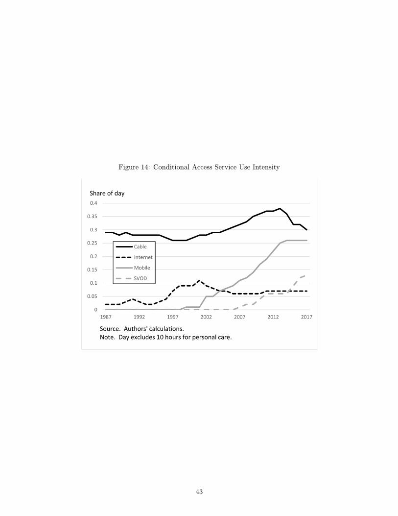
Figure 14: Conditional Access Service Use Intensity

0

0.05

0.1

0.15

0.2

0.25

0.3

0.35

0.4

1987 1992 1997 2002 2007 2012 2017

Cable

Internet

Mobile

SVOD

Share of day

Source.  Authors' calculations.Note.  Day excludes 10 hours for personal care.

43

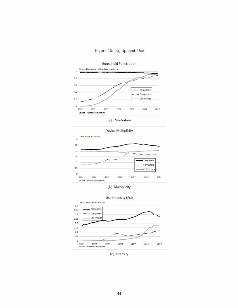
Figure 15: Equipment Use

(a) Penetration

(b) Multiplicity

(c) Intensity

44