Accounting for Needs in Cost Sharing∗

Etienne Billette de Villemeur

Universite de Lille and Chaires Universitaires Toussaint Louverture

Justin Leroux

HEC Montreal, CIRANO and CRE

This version: September 8, 2016

Abstract

We introduce basic needs in cost-sharing problems so that agents with higher

needs are not penalized, all the while holding them responsible for their con-

sumption. We characterize axiomatically two families of cost-sharing rules, each

favoring one aspect—compensation or responsibility—over the other. We also

identify specific variants of those rules that protect small users from the cost

externality imposed by larger users. Lastly, we show how one can implement

these schemes with realistic informational assumptions; i.e., without making

explicit interpersonal comparisons of needs and consumption.

Keywords: Cost Sharing; Needs; Responsibility; Liberal Egalitarianism.

JEL code: D63.

∗We thank seminar participants at the Montreal Environmental and Resource Economics Work-

shop, Universite de Lille, the annual Journees Louis-Andre Gerard-Varet (Aix-Marseille), Univer-

sity of Hawaii, University of Texas at Austin, Toulouse School of Economics, Universite Quisqueya

(Port-au-Prince), University of Ottawa, and University of Winnipeg. We also thank Ariel Di-

nar, Herve Moulin, Marcus Pivato, Yves Sprumont and Max Stinchcombe. Financial support from

FRQSC is gratefully acknowledged.

1

1 Introduction

Most allocation mechanisms rely only on demand, that is to say on what biologists

would call wants. We argue in favor of introducing objective characteristics to com-

plement this subjective input. Specifically, we study pricing formulas that do not

penalize agents with higher needs.

Some public utilities, like water and wastewater services, are essential to achieving

a decent standard of living. In a society where households differ in terms of their basic

needs for utility services, these should be taken into account when setting utility rates.

In practice, commendable efforts have been made in this regard, with rate schedules

typically taking the form of multi-part tariffs (block pricing), including discounts given

to households with higher needs (for the case of water supply in the US, see AWWA,

2012). These discounts can take the form of a rebate to low-income households, which

is subsidized by a higher overall rate structure. Alternatively, increasing-block rate

schedules subsidize the lowest block through rate premiums for large users, hence

affording all households a low rate to meet basic needs. In the case of water services,

this also addresses the issue of resource conservation.1 Nevertheless, while these

practices recognize the fact that some households should be subsidized, the design

of such subsidies, both in shape and in magnitude, is largely left to rule-of-thumb

considerations.2

Our aim is to design a pricing scheme that does not penalize agents for having

higher needs. As we shall see below, social transfers to finance the basic needs of the

poor actually cannot achieve this. This is because what will remain to be paid will

necessarily depend on their needs. Alternatively, adjusting prices to reflect differences

in income may be unfeasible, either because it is too informationally costly or simply

illegal. In fact, our objective is not quite the same as making essential consumption

’affordable’; we merely require that agents with higher needs are not at a disadvantage

in their ability to achieve a given welfare level.

We develop a framework to formally take matters of partial responsibility into

account when devising rates for utility services, which we will assume to be water

1The recent move towards ”water budget-based rates” or, more accurately, to ”sustainable”rate design in some U.S. municipalities reflects these concerns (Barr and Ash, 2015; Barraque andMontginoul, 2015; Dinar and Ash, 2015)

2For example, the M1 Manual of the American Water Works Association, a highly regardedreference by North American water utilities, gives surprisingly little guidance on how to determinerate blocks: “Generally, rate blocks should be set at logical break points.” (AWWA, 2012, p.107)

2

services to fix ideas.3 Each agent is summarized by her water consumption and her

basic water needs, which may differ from one agent to the next. For instance, one

can think of agents as being households of possibly different sizes. We take the view

that agents should not be penalized for their needs, but are fully responsible for their

consumption beyond those needs.

Our approach builds on the axiomatic framework of liberal egalitarianism, which

aims at compensating differences in “non-responsibility” characteristics while reward-

ing differences in characteristics under the agents’ control. Classically, agents are

deemed responsible for their effort but have no control over their talents. Here,

agents have no control over their basic water needs—say, 50 liters of clean water per

day (Gleick, 1996)—but are responsible for their consumption beyond that amount.

Thus, water consumption is a ’hybrid’ characteristic of sorts: the portion required

to meet basic needs falls into the non-responsibility category, whereas the remainder

falls into the sphere of responsibility.

A general theme of that literature is that the two desiderata of compensation and

reward are incompatible (Bossert, 1995; Bossert and Fleurbaey, 1996; Cappelen and

Tungodden, 2006). Accordingly, one must set less ambitious goals for redistributive

policies. This is typically done by giving priority to one ideal—compensation or re-

ward—while limiting the scope of the other (Fleurbaey 2008, and references therein),

leading to the Egalitarian Equivalent and Conditional Equality solutions, respec-

tively. Likewise, we characterize two polar families of solutions: Conditional Equality

solutions emphasize responsibility for excessive usage (Theorem 1) while Egalitarian

Equivalent solutions stress compensation for differences in needs (Theorem 4).

Contrasting with previous results, the solutions we obtain are not unique because

they depend on two additional dimensions that the literature is currently not equipped

to handle: how to account for ’hybrid’ characteristics and how to account for cost

externalities. The latter is embodied by the nonlinearity of the cost function, which

links the agents through the requirement of balancing the budget. Regarding the for-

mer, each family of solutions will produce different solutions whether one measures

responsibility in terms of consumption (q) beyond needs (q), formally q−q, or in terms

of its fraction relative to one’s own needs, (q − q) /q, for example. We call these views

absolute responsibility and relative responsibility, respectively. When welfare can be

3Our analysis applies to all utilities necessary for a decent standard of living, including electricityservices.

3

evaluated by means of a (common) utility function—i.e., when agents differ only in

their needs—and when the responsibility measure is chosen so as to reflect the actual

welfare of the agents—a more sophisticated exercise—Conditional Equality solutions

are actually compatible with a much stronger compensation requirement than when

responsibility is computed arbitrarily (Theorem 3). This implies that, when differ-

ences in needs summarize the relevant differences across agents, sufficient knowledge

of the utility function can afford greater compatibility between the desiderata of com-

pensation and reward, a sharp contrast with existing results in the literature on liberal

egalitarianism.

Even with a specific view on responsibility, much freedom remains regarding how

to account for cost externalities within each family of solutions. Indeed, the par-

tial responsibility approach determines what portion of the total cost is devoted to

meeting basic needs. How to split the remainder—for which agents are deemed re-

sponsible—falls into the realm of cost-sharing theory. In principle, any cost-sharing

rule can be associated with each family of solutions and with each responsibility view.

However, given the nature of the service at hand, when costs are convex we posit an

axiom that protects parsimonious users from the cost externality caused by wasteful

users. When costs are concave, so that there are economies of scale, we ask ’small

users’ to fully benefit from a further reduction in their consumption. This charac-

terizes unique solutions: the serial (Moulin and Shenker, 1992) and decreasing-serial

(de Frutos, 1998) cost-sharing variant of each family of solutions, respectively when

costs are convex or concave (Propositions 2-5).

Lastly, we show how one can implement the above schemes with realistic informa-

tional assumptions; i.e., without making explicit interpersonal comparisons of needs

and consumption, which would prove very difficult and possibly counterproductive

for all but very small populations. In particular, we use household size as a proxy

for needs and denote by qs the needs of a household of size s. Using aggregate infor-

mation to summarize distributional aspects, we design rate schedules that otherwise

explicitly depend on the sole individual characteristics of households.

For instance, consider affine costs of the form C(Q) = F+cQ, with F, c > 0, where

Q is the aggregate demand of the population.4 When responsibility is measured by

4Such a cost structure is typical of water services, which exhibit high fixed costs (infrastructure)and low marginal costs (electricity for pumping and chemicals for treatment).

4

absolute responsibility, q−qs, the decreasing serial conditional equality solution5 yields

the following rate schedule for households of size s:

F + cQ

N+ c (q − qs) , (1)

where Q is the quantity needed to cover the needs of the entire population, and N

is the total number of households. In addition to splitting the fixed cost equally,

this rate schedule shares the cost of the population’s needs equally before pricing

consumption at marginal cost (minus a rebate equal to the cost of meeting one’s own

needs).

The rate schedule changes significantly under the relative responsibility view. As-

suming responsibility is identically distributed across types, we obtain the following

rate schedule for households of size s:

F

N+

c

qs/(Q/N

)q (2)

The result is still a two-part tariff but one where only the fixed cost is split equally. No

rebate is granted, and consumption is priced at a rate that is inversely proportional

to one’s needs.

By contrast, the family of egalitarian equivalent solutions is based on utility com-

parisons with households having a hypothetical reference level of needs, q0, chosen

by the planner. Under the decreasing serial egalitarian equivalent solution, which

emphasizes compensating differences in needs over responsibility, the rate schedule

for households of size s is as follows:

F

N+ cq + [us (q, qs)− us (q, q0)]− 1

N

∑t

∫ ∞z=0

[ut (z, qt)− ut (z, q0)]nt (z) dz,

where us (q, qs) is the utility of a representative household of size s and where ns (q)

is the density of households that are consuming q units in the distribution of size-s

households. The cost-sharing portion of the schedule, FN

+ cq, splits the fixed cost

equally and prices consumption at marginal cost. Needs are completely absent from

that component. However, they enter in the remaining, redistributive portion to

5As mentioned, the decreasing serial cost-sharing rule is the more appropriate for concave costs.

5

ensure that heterogeneity in needs does not drive differences in welfare.

The remainder is organized as follows. The next section offers a brief discussion

of the related literature. Section 3 presents the formal model. In Section 4, we

take the cost-sharing rule as given in order to focus on our contribution; namely, the

introduction of essential needs in cost-sharing problems. We then introduce a specific

property of the rate function, which aims at protecting small users while still holding

them accountable, and show how doing so calls for adopting a specific underlying

cost-sharing rule depending on the convexity of the externality (Section 5). Finally,

we show in Section 6 how these abstract formulas actually boil down to specific two-

part tariffs for which we provide an explicit and complete determination using only

coarse information on characteristics of the population.

2 Related Literature

Liberal egalitarianism. Our work expands the literature on liberal egalitarianism

in two ways. First, we extend the theory to settings with externalities. To our

knowledge, the only other effort in this direction is Billette de Villemeur and Leroux

(2011), which tackles the issue of global climate change and the design of transfer

schemes between countries to account for their responsibility in current emissions

and, possibly, their non-responsibility in past emissions. Externalities are introduced

through a (nonlinear) damage function, but basic needs are absent from their setting.

Our second contribution has to do with our consideration of a characteristic—here,

consumption—for which one is both partly responsible and partly non-responsible.

Ooghe and Peichl (2014) and Ooghe (2015) very recently introduced the notion of

’partial control’ over some characteristics to handle different degrees of responsibility

in any given characteristic. According to this ’soft cut’, an agent may be responsible

for, say, only 30% of his intellectual skills, the remainder being attributable to inborn

abilities or environmental factors. Our view of consumption as a hybrid characteristic

differs from theirs in that we deem households fully non-responsible for the portion

aimed at satisfying their needs, but fully responsible for the remaining portion, viewed

as discretionary.

Needs. Economists have been aware for quite some time that the welfare interpre-

tation of income inequality measures is problematic (see among others Garvy, 1954;

6

David, 1959; Morgan, 1962). How to account for differences in ability and needs is still

the topic of lively discussions in public economics, in particular in the literature on

taxation, but not only (e.g., Mayshar and Yitshaki, 1996, Trannoy, 2003, Duclos et al.

2005, Duclos and Araar 2007). Ebert (1997) adopts an axiomatic approach to discuss

the comparison of income distributions when the population consists of heterogeneous

households. Observing that economic growth had done very little for the poorer half

of the third world population, some economists at the World Bank have pointed out

the importance of looking at basic needs (Streeten and Burki, 1978; Streeten, 1979;

Hicks and Streeten, 1979). Similarly, rather than being concerned with the ’afford-

ability’ of services to low-income households, as do most approaches to rate setting,

we focus on the material—as opposed to the financial—needs of households.

Fair division. Despite mounting empirical evidence suggesting that needs are a

relevant ingredient of fairness (Konow, 2001; Traub et al, 2005; Schwettman, 2012),

the literature on fair division has only recently considered basic needs in a formal

fashion. Specifically, although in a setting different from ours, Bergantinos et al.

(2012) and Manjunath (2012) modify the classical rationing problem—where a fixed

social endowment must be divided among several recipients—to account for a minimal

requirement. There, agents are indifferent between receiving less than this minimal

share and receiving nothing.

Because we ask for full cost recovery, the relevant strand of the fair division liter-

ature is that of cost sharing. Yet, this literature does not explicitly address the issue

of basic needs. The closest work in that direction lead to sharing rules that protect

small users when costs are convex (Moulin and Shenker, 1992) or guarantee that small

users will indeed be rewarded from reducing their consumption to the tune of their

effort (de Frutos, 1998). We build upon these two sharing rules to complement our

approach (Section 5).

3 Accounting for Needs

The Model. Let N = {1, ..., n} be the set of agents. Agent i consumes a quantity

qi ≥ 0 of water. Serving all of the agents’ demands Q =∑n

i=1 qi costs C (Q) ≥ 0,

where C is an increasing cost function.6

6We use the following convention: by ’increasing’ we mean ’strictly increasing’. We use theterm ’non-decreasing’ when the monotonicity is not strict. Similarly, by ’positive’ we mean ’strictly

7

Full cost recovery is essential to the sustainability of the infrastructure.7 Thus,

we require that the agents’ water bills, xi’s, cover the total cost:

n∑i=1

xi ≥ C (Q) . (3)

We denote by Γ the class of cost functions. Our aim is to define appropriate formulas

to compute the agents’ bills. We restrict ourselves to the case where no profits are

made, owing to the public nature of the service, so that the budget constraint (3) is

binding.

The needs of agent i, in terms of water use, are denoted qi ≥ 0. We adopt a

quasi-linear setup, where agent i’s utility level is defined by:

Ui (qi, qi, x) = ui (qi, qi)− xi.

The utility function ui, which is possibly agent specific, is defined on D ≡{

(x, y) ∈ R2+|x ≥ y

}.8

It is assumed to be increasing in qi and decreasing in qi. We denote by Υ the class

of utility functions. When agents consume exactly their needs, they share a common

utility level u that, without loss of generality, we can set to zero. Formally,

ui (qi, qi) ≡ 0, ∀qi ≥ 0,∀i ∈ N.

Defining responsibility. Our aim is to design a pricing rule that does not

penalize agents with higher needs while taking individual responsibilities into account.

In order to do so, we must define the sphere of responsibility of the agents. We consider

that agents are not responsible for their essential needs, qi, but are responsible for any

consumption beyond those needs. The extent of their responsibility can be measured

in many different ways. For the sake of generality, we define a real-valued function,

positive’, and use ’nonnegative’ when zero is not excluded.7For example, while it remains an empirical matter whether pricing water actually leads to

economic efficiency in practice, it is widely recognized that full cost recovery is essential to the sus-tainability of the infrastructure (Massarutto, 2007; AWWA, 2012; Canadian Water and WastewaterAssociation, 2015) and is “a key preoccupation” of many OECD countries (OECD, 2010). Still in thecontext of water services, Massarutto (2007) identifies three important benefits of recovering coststhrough the pricing structure: to “ensure the viability of water management systems”, to “maintainasset value over time”, and to “guarantee the remuneration of inputs”.

8Because we consider qi to represent agent i’s essential needs, it is a lower bound to her con-sumption.

8

r1(q1, q1)

r 2(q

2,q

2)

q

q

q2

q2

q1 q1

C(Q

)

C(Q

)eq

ual re

spon

sibili

ty(a

bsolut

e)

equal responsib

ility (re

lative)

Figure 1: Responsibility is measured from q. Given the position of q relative to qin this figure, if responsibility is defined as qi − qi (absolute responsibility) agent 1 isconsidered to bear more responsibility than agent 2 in her discretionary consumption.If it is defined as (qi − qi)/qi (relative responsibility), the reverse holds.

r(qi, qi), defined on D, which is increasing in water consumption qi, non-increasing

in needs qi, and normalized to zero when qi = qi. When no confusion is possible,

we abuse notations slightly by denoting ri = r(qi, qi). We denote by R the class of

responsibility functions.

A consumption-needs profile (or simply a profile) is a list of n consumption-needs

pairs that we shall denote (q, q) ∈ Dn, abusing notations slightly.9

Rate functions and cost-sharing rules. Having defined the notion of re-

sponsibility, we can now share the total cost according to the responsibility profile,

r ≡ (r1, r2, ..., rn). In doing so, cost-sharing rules (ξ) will allow us to highlight the dis-

tinction between the handling of the production externality—governed by the shape

of the cost function—and the redistribution problem that follows from taking essen-

9We shall adopt the convention that boldface type refers to the vector of the relevant variables.E.g., q = (q1, ..., qn) and q = (q1, ..., qn).

9

tial needs into account. We ultimately provide pricing formulas, that we shall refer

to as rate functions (x).

Formally, let C(q, q) stand for the portion of the cost for which the population is

considered to be responsible, once needs are accounted for. The principles of liberal

reward and compensation will guide us in defining C(q, q). A cost-sharing rule is a

mapping that splits this portion of the cost across users: ξ : Rn × Γ → Rn, such

that∑

i ξi (r, C) = C(q, q). By contrast, a rate function takes all the information in

the economy into account and is a mapping x : Dn × R × Υ × Γ → Rn such that∑i∈N xi(q, q, r, u, C) = C(Q) where C(Q) is the total cost to be covered.

Section 6 will be devoted to obtaining explicit formulas based on illustrative ex-

amples. Until then, fix the cost function, C, the common utility function, u, and the

responsibility function, r. As a result, we abuse notations slightly and write x(q, q)

instead of the more cumbersome x(q, q, r, u, C).

4 Fair Treatment

4.1 Interdependence and Anonymity

A natural and seemingly minimal fairness requirement is that two agents with iden-

tical needs face the same pricing schedule:

Axiom. (Equal Rate Schedule for Equal Needs, ERSEN)

The functions qi 7→ xi (q, q) and qj 7→ xj (q, q) must be identical whenever qi = qj.

As it turns out, however, ERSEN is unfeasible:

Theorem 1. No rate function satisfies ERSEN unless the cost function is linear.

Proof. Let (q, q) ∈ Dn such that qi = qj for some i 6= j. By budget balance, the rate

schedule of agent 1, f : q′i 7→ xi ((q′i,q−i) , q), writes as follows:

f (q′i)− f (qi) = C (Q− qi + q′i)− C (Q) ∀q′i ∈ [qi,+∞). (4)

By ERSEN, the function f cannot depend on qj, so that :

f (q′i)− f (qi) = C(Q− qi + q′i − qj + q′j

)− C

(Q− qj + q′j

), (5)

10

for all(q′i, q

′j

)∈ [qi,+∞)× [qj,+∞). Taken together, Expressions (4) and (5) yield:

C (Q− qi + q′i)− C (Q) = C(Q− qi + q′i − qj + q′j

)− C

(Q− qj + q′j

), (6)

for all(q′i, q

′j

)∈ [qi,+∞)× [qj,+∞).

Already, Expression (6) suggests that C increases at a constant rate. We prove

this formally by rewriting the expression as a Cauchy functional equation. Let h > 0

and consider q′i = qi + h and q′j = qj + h. Expression (6) becomes:

C (Q+ h)− C (Q) = C (Q+ 2h)− C (Q+ h) ∀h ≥ 0. (7)

Rearranging and defining g : h 7→ C (Q+ h) on R+ yields:

g (2h) + g (0) = 2g (h) ∀h ≥ 0. (8)

Expression (8) must hold for all h and thus defines a functional equation in g. This is

a well-known Cauchy equation (Aczel, 1967), which requires g—and therefore C—to

be linear in its argument. Having started from an arbitrary profile (q, q), linearity

follows on the full domain of C.

ERSEN effectively requires that the rate schedule an agent faces depends only

on the profile of needs, but not on the consumption vector. However, this ignores

the interdependence that exists between agents through the cost function. Theorem 1

makes it clear that, if this interdependence is not accounted for, rate schedules cannot

be determined ex ante, on the sole basis of needs.10 It follows that we must depart

from the simplistic view according to which agents can ignore the impact they have

on others, as is assumed to be the case under perfect competition, for instance. We

therefore adopt a more comprehensive view in which bills depend explicitly on the

entire profile of consumption and needs.

Moreover, just as individuals cannot be considered in isolation, essential needs can-

not be handled separately from consumption beyond them. Financing the provision

of essential needs (Q) through, say, the income tax—and having agents pay for Q− Qthrough a pricing scheme that depends on the sole qi’s, ignoring the qi’s—would not

solve our problem. In fact, agents’ bills would be required to finance C (Q)−C(Q),

10For a general proof of the incompatibility between budget balance and equal treatment of equals,albeit when needs are absent, see Billette de Villemeur and Leroux (2016).

11

which depends explicitly on Q. This is in contradiction with the fact that once

essential needs have been financed, they can be ignored in pricing the remaining

consumption.

Even worse, if agents’ bills were to depend solely on the qi’s, an agent whose

needs happened to increase but whose consumption remained unchanged would end

up paying the same amount despite a lower responsibility in consumption. This

can lead to situations where one agent ends up paying more than another despite

having both lower responsibility and higher needs. Indeed, consider any i such that

qi > qj > qj for some j 6= i. Nevertheless, her needs can increase to some level

qi ∈ (qj, qi) such that ri < rj even though she ends up paying more than j (because

qi > qj).

In addition, budget balance would necessarily be violated. Suppose the needs

of the population happen to decrease, while again consumption remains unchanged.

Then, the portion of costs that must be financed through pricing—C (Q)−C(Q)—increases

and revenue requirements are no longer met.

We shall thus stick to our encompassing approach, which aims at financing the

total cost, C (Q), by accounting jointly for the qi’s and the qi’s.

The fairness requirement we shall adopt is that the rate function satisfies anonymity.

Formally, we shall require that, for any permutation of the agents π : N → N :

xπ(i) (qπ; qπ) = xi (q; q) for all i ∈ N ,

where qπ (resp. qπ) is the vector of consumption (resp. needs) after permutation of

the agents along π.

Remark 1. Anonymity implies the equal treatment of equals: (qi, qi) = (qj, qj) =⇒xi (q; q) = xj (q; q). Two users with identical needs and identical consumption must

pay the same bill.

4.2 The Reward Principle: Responsibility Axioms

The general idea behind the reward principle is that conservative users should be

rewarded in the form a lower bill. Of course, if needs are accounted for, whether con-

sumption is moderate or not is not measured by considering only actual consumption,

but on the basis of r (qi, qi).

12

A minimal requirement in terms of responsibility is that the portion of costs

resulting from consumption above and beyond the needs of the population, C(Q) −C(Q), be distributed to users according to their contribution to this cost. This

leads us to introducing a cost-sharing rule, ξ, to split C(Q) − C(Q) according to

the responsibility profile, r. Keeping with the desideratum of anonymity, we shall

consider only symmetric cost-sharing rules:

ξ(r, C − C(Q)

)is a symmetric function of the variables ri, i ∈ N.

The function ξ embodies how we want to hold agents accountable for their consump-

tion.11 Given ξ, the following axioms specify how responsibility is assigned, and are

presented in decreasing order of stringency.

Axiom. (Shared Responsibility, SR)

xk (q, q)− xk (q, q) = ξk(r, C − C(Q)) ∀k ∈ N

A less demanding axiom consists in sharing C(Q) − C(Q) according to ξ only

when all agents have equal needs.

Axiom. (Shared Responsibility for Uniform Needs, SRUN)

[qi = qj,∀i, j ∈ N ] =⇒[xk(q, q)− xk(q, q) = ξk(r, C − C(Q)),∀k ∈ N

]Finally, an even less demanding axiom consists in sharing costs according to ξ

only when the needs of all are identical and equal to a reference level, q0 ∈ R+.

Axiom. (Shared Responsibility for Reference Needs, SRRN)

For some reference level of needs, q0 ∈ R+:

[qi = q0, ∀i ∈ N ] =⇒ [xk(q, q0)− xk(q0, q0) = ξk(r0, C − C(nq0)), ∀k ∈ N ]

where q0 = (q0, q0, ..., q0) and r0,i = r (qi, q0) for all i ∈ N .

11If needs were not an issue, we would be back to the classical cost-sharing framework whereξ (q, C) alone defines the shares to be paid (see Moulin, 2002, for a thorough survey).

13

4.3 The Compensation Principle: No Responsibility for One’s

Needs

Throughout, we take the view that agents are not responsible for their needs. Ideally,

difference in needs should not drive differences in welfare:

Axiom. (Group Solidarity, GS)

For any i ∈ N and any two profiles (q,q) and (q,q′) such that q′i 6= qi and q′j = qj

for all j ∈ N\ {i} , then

[ui (qi, q′i)− x′i]− [ui (qi, qi)− xi] =

[uj(qj, q

′j

)− x′j

]− [uj (qj, qj)− xj] ,

for all j ∈ N , where x = x (q,q) and x′ = x (q,q′).

Another, weaker approach consists in requiring that when two agents bear an

equal responsibility, their welfare should be equal:

Axiom. (Equal Welfare for Equal Responsibility, EWER)

ri = rj =⇒ ui (qi, qi)− xi = uj (qj, qj)− xj

We shall also consider a weaker axiom, which consists in requiring equality of

welfare only if all agents bear an equal responsibility:

Axiom. (Uniform Welfare for Uniform Responsibility, UWUR)

[ri = rj,∀i, j ∈ N ] =⇒ [ui (qi, qi)− xi = uj (qj, qj)− xj,∀i, j ∈ N ]

An even weaker axiom consists in having the same requirement only if this common

level of responsibility is equal to a reference level:

Axiom. (Uniform Welfare for Reference Responsibility, UWRR)

For some reference responsibility level, r0 ∈ R+ :

[r (qi, qi) = r0,∀i ∈ N ] =⇒ [ui (qi, qi)− xi = uj (qj, qj)− xj,∀i, j ∈ N ]

Finally, we shall say that a rate function satisfies Uniform Welfare for Minimal

Consumption (UWMC ) if it satisfies UWRR with reference responsibility level

r0 = 0.

14

4.4 Pricing Mechanisms

We now turn to the design of pricing mechanisms. The principles of responsibility

and compensation will determine how to allocate the cost of meeting the needs of the

population, C(Q), but not only. As we shall see, these principles will also interact

with how the cost C (Q)−C(Q), is to be split. The two portions of the cost cannot

be considered in isolation.

Conditional Equality: SR+UWRR

Turning first to rate functions that prioritize holding agents responsible for their

consumption, we identify the strongest compensation axioms compatible with SR.

We find that UWRR and SR jointly characterize a family of rate functions, which we

call Conditional Equality solutions,12 that is parametrized by the choice of a reference

responsibility level, r0:

Theorem 2. A rate function x satisfies SR and UWRR if and only if x = xCE

where, for some reference level r0 > 0,

xCEi (q, q) =C(Q)

n+ ξi

(r, C − C(Q)

)+ ui

(q0i , qi

)− 1

n

∑j∈N

uj(q0j , qj

),

for all i ∈ N , where q0i is defined by r (q0

i , qi) = r0.

Proof. In Appendix A.1.

A special variant of the Conditional Equality solutions consists in choosing zero

responsibility as a reference: q0 = q. This implies charging households the same

fee to meet their own needs, whatever those needs may be. Should they choose to

consume more, they would bear the consequences according to the cost-sharing rule

in effect.

Corollary 1. The unique rate function satisfying SR and UWMC is the following:

xCE0i (q, q) =

C(Q)

n+ ξi(r, C − C(Q)) for all i ∈ N .

12The name reflects the fact that this family of solutions is reminiscent of the conditional equalitysolution in Fleurbaey (1995) in a different context.

15

A limit of xCE0 is that compensation for needs is established on the basis of a

single scenario which is unlikely to ever arise. However, it possesses the advantage of

not requiring knowledge of the utility function.

Theorem 2 is generically tight because xCE generically does not satisfy the stronger

compensation axiom UWUR. The only exception is when the agents share a common

utility function and the responsibility function, r, reflects the utility derived by the

agents:

Proposition 1. xCE does not satisfy UWUR unless the following two assertions

are true:

(1) all agents share a common utility function; i.e., ui = u ∈ Υ, for all i ∈ N(2) the responsibility function co-varies with agents utility; i.e., r = ρ ◦ u, for some

increasing function ρ : R→ R+.

Proof. In Appendix A.2.

In fact, when the conditions of Proposition 1 are true, SR is even compatible

with the stronger compensation axiom EWER. Together, they characterize a unique

solution:

Theorem 3. If ui = u ∈ Υ, for all i ∈ N and if r = ρ ◦ u, for some increasing

function ρ : R→ R+, a rate function x satisfies EWER and SR if and only if

x ≡ xCE0

Proof. In Appendix A.3.

The above result applies only to specific circumstances: agents differ only in their

needs, but not in their preferences. A remarkable feature of the above characteriza-

tion is that it does not require specifying a reference responsibility level, although it

obviously requires knowledge of the (common) utility function.13

Theorem 3 is a tight characterization because SR is incompatible with the strongest

solidarity axiom, GS, as Theorem 4 below implies.

13Knowledge of the common utility function u is merely required to check whether the theoremapplies, not to compute cost shares. In particular, cardinal information about preferences is notneeded.

16

Egalitarian Equivalence: GS+SRRN

We now turn to rate functions that prioritize negating the impact of differences in

needs on welfare. Axiom GS embodies this desideratum. We show that GS together

with SRRN determine a family of rate functions, which we call the Egalitarian

Equivalent solutions,14 that is parametrized by a reference level of needs, q0:

Theorem 4. A rate function x satisfies GS and SRRN if and only if x = xEE

where, for a given reference level of needs, q0 > 0,

xEEi (q, q) =C(nq0)

n+ ξi (r0, C − C (nq0))

+ [ui (qi, qi)− ui (qi, q0)]− 1

n

n∑k=1

[uk (qk, qk)− uk (qk, q0)] ,

for all i ∈ N , where r0 = (r (q1, q0) , r (q2, q0) , ..., r (qn, q0)).15

Proof. In Appendix A.4.

xEE measures responsibility relative to the common reference level, q0: ri,0 =

r (qi, q0) and splits costs accordingly. Differences between actual needs and the refer-

ence level are compensated for so as to preserve the relative welfare distribution.

The characterization is tight, in the sense that the Egalitarian Equivalent solution

does not satisfy stronger responsibility axioms. This can be shown by considering a

profile (q, (q1, q1, ..., q1)) ∈ Dn such that q1 6= q0 to obtain that SRUN is not satisfied.

The formal proof can be found in Appendix A.5.

Remark 2. The cost-sharing portion of the transfer, (1/n)C(nq0)+ξi (r0, C − C (nq0)),

is driven by the consumption profile of the agents and by the cost structure, but is

actually independent of individual needs. By contrast, the redistributive component

of the bill, [ui (qi, qi)− ui (qi, q0)] − (1/n)∑n

k=1 [uk (qk, qk)− uk (qk, q0)], is based on

the benefits the agents derive from consumption and is independent of costs.

Remark 3. Whenever needs summarize all relevant differences across agents so that

they share a common utility function u, whatever the value of q0, the Egalitarian

14The name reflects the fact that this family of solutions is reminiscent of the egalitarian equivalentallocations in the seminal contribution by Pazner and Schmeidler (1978).

15Given the domain of definition of the utility functions, xEE is well defined only on the set{(q, q) ∈ Dn|mini qi ≥ q0} .

17

Equivalent solution fully addresses the issue of differences in needs whenever con-

sumption is uniform. Formally, if q1 = q2 = ... = qn, then ui (qi, qi) − xEEi (q, q) =

uj (qj, qj)− xEEj (q, q) for all i, j ∈ N . In other words, under xEE, any differences in

utility levels are attributable to differences in consumption.

Remark 4. The fact that the Conditional Equality solutions satisfy weaker compen-

sation axioms does not mean that the Egalitarian Equivalent solutions are more re-

distributive. Indeed, for the latter, the parameter q0 dictates both the portion of the

cost to be shared in an egalitarian fashion and how differences in needs are accounted

for. In particular, when q0 = 0, the portion of costs to be split equally under xEE is

nil—C (nq0) /n = 0—and users are held responsible for their whole consumption. By

contrast, xCE always splits equally the portion of costs corresponding to the needs of

the population: C(Q).

5 Protecting small users while holding them re-

sponsible

5.1 Convex Costs

We introduce an axiom that aims to protect parsimonious users from the cost ex-

ternality caused by wasteful users: An agent who increases her responsibility level

cannot lead consumers with lower responsibility to pay a higher amount.

Axiom. (Independence of Higher Responsibility, IHR) For all (q, q) and

(q′, q′) such that q′ = q and r′ ≥ r. For all i ∈ N, define L (i) = {j ∈ N s.t. rj ≤ ri}the set of users with lower responsibility than i. Then,

{r′j = rj for all j ∈ L (i)

}=⇒

{ξj(r′, C − C

(Q′))

= ξj(r, C − C

(Q))

for all j ∈ L (i)}.

Remark 5. Note that for a given profile (q, q), such that qi > qj and qi > qj for some

i and j, then one can find two functional forms r and r such that

r (qi, qi) ≥ r (qj, qj) and r (qi, qi) < r (qj, qj) .

18

Hence, the identity of consumers with a smaller responsibility depends on how re-

sponsibility is measured; i.e., upon the specific functional form for r (Figure 1).

Serial Conditional Equality

Recall that r (·, qi) maps an agent’s consumption to her responsibility level, given

her needs. Define the inverse of this function, gi (·) = (r)−1 (·, qi), which maps a

responsibility level to the corresponding consumption level given the needs of the

agent.

Proposition 2. The unique rate function satisfying UWMC, SR and IHR is the

following:

xSCE0i (q, q) =

C(Qi)

(n− i+ 1)−

i−1∑k=1

C(Qk)

(n− k) (n− k + 1)for all i ∈ N ,

where, for all k ∈ N ,

Qk =k−1∑i=1

qi +n∑i=k

gi (rk) ,

where the set of agents is ordered so as to have r1 ≤ r2 ≤ ... ≤ rn.

Proof. In Appendix B.1.

Remark 6. xSCE0 amounts to applying the serial cost-sharing rule to responsibility

levels. In fact,

xSCE0i (q, q) =

1

nC(Q)

+i∑

k=1

1

n− k + 1

[C(Qk)− C

(Qk−1

)],

with Q0 = Q . This is of notable interest because the serial cost-sharing rule is known

for its strong incentives properties (Moulin and Shenker, 1992).

Notice that a higher responsibility level leads to a higher bill: ri ≥ rj implies

xSCE0i (q, q) ≥ xSCE0

j (q, q) because

Qk+1 − Qk =n∑

i=k+1

[gi (rk+1)− gi (rk)] ≥ 0.

19

Serial Egalitarian Equivalence

Proposition 3. A rate function x satisfies GS, SRRN and IHR if and only if

x = xSEE where, for a given reference level of needs q0 > 0,

xSEEi (q, q) =C(Qi)

(n− i+ 1)−

i−1∑k=1

C(Qk)

(n− k) (n− k + 1)

+ [ui (qi, qi)− ui (qi, q0)]− 1

n

n∑k=1

[uk (qk, qk)− uk (qk, q0)]

for all i ∈ N , where Qk =∑k

l=1 ql + (n− k) qk with the set of agents ordered so as to

have q1 ≤ q2 ≤ ... ≤ qn.16

Proof. In Appendix B.2.

Remark 7. The expression for xSEE is independent of the form of responsibility.

Remark 8. xSEE amounts to applying the serial cost-sharing rule directly to con-

sumption, along with transfers to compensate for differences in needs. In fact,

xSEEi (q, q) =1

nC

(n inf

jqj

)+

i−1∑k=1

1

n− k

[C(Qk+1

)− C

(Qk)]

+ [ui (qi, qi)− ui (qi, q0)]− 1

n

n∑k=1

[uk (qk, qk)− uk (qk, q0)] .

Note that the compensation terms may affect the well-known incentives properties of

the serial cost-sharing rule.

At first blush, the expressions of xSCE0 and xSEE may seem similar, with xSEE

having an additional compensation term. However, note that agents are ordered

according to their consumption under xSEE but are ordered according to their re-

sponsibility level under xSCE0. Also, the Qk’s that enter in the cost-sharing portion

stand for different aggregate consumption levels. In particular, xSEE applies the se-

rial cost-sharing rule directly on consumption levels, with needs appearing only in

the compensation portion. By contrast, xSCE0 applies the serial cost-sharing rule to

responsibility levels which, by design, take individual needs into account.

16xSEE is well defined only on the subdomain {(q, q) ∈ Dn|mini qi ≥ q0} .

20

5.2 Concave Costs

With increasing marginal cost, we wished to protect users with smaller responsibility

levels from bearing a high marginal cost due to the presence of ’large users’. By con-

trast, when the technology exhibits increasing returns to scale, we want ’small users’

to fully benefit from a further reduction in their consumption. It follows that larger

users never benefit from the effort of smaller users in reducing their consumption.

Axiom. (Independence of Lower Responsibility, ILR) For all (q, q) and

(q′, q′) such that q′ = q and r′ ≤ r. For all i ∈ N, define H (i) = {j ∈ N s.t. rj ≥ ri}the set of users with higher responsibility level than i. Then,

{r′j = rj for all j ∈ H (i)

}=⇒

{ξj(r′, C − C

(Q′))

= ξj(r, C − C

(Q))

for all j ∈ H (i)}.

Decreasing Serial Conditional Equality

Proposition 4. The unique rate function satisfying UWMC, SR and ILR is the

following:

xDSCE0i (q, q) =

C(Qi)

i−

n∑k=i+1

C(Qk)

k (k − 1)for all i ∈ N ,

where, for all k ∈ N ,

Qk =k∑l=1

gl (rk) +n∑

l=k+1

ql,

where the set of agents is ordered so as to have r1 ≤ r2 ≤ ... ≤ rn.

Proof. In Appendix B.3.

Remark 9. xDSCE0 amounts to applying the decreasing serial cost-sharing rule to

responsibility levels in order to split the associated costs. In fact,

xDSCE0i (q, q) =

1

nC(Qn)−

n−1∑k=i

1

k

[C(Qk+1

)− C

(Qk)]

with Q1 = Q. Like the serial rule, the decreasing serial cost-sharing rule is also known

for its strong incentives properties (de Frutos, 1998).

21

Note that a higher responsibility level indeed leads to a higher bill: qri ≥ qrj implies

xDSCE0i (q, q) ≥ xDSCE0

j (q, q) because

Qk+1 − Qk =k∑l=1

[gl (rk+1)− gl (rk)] ≥ 0.

Decreasing Serial Egalitarian Equivalence

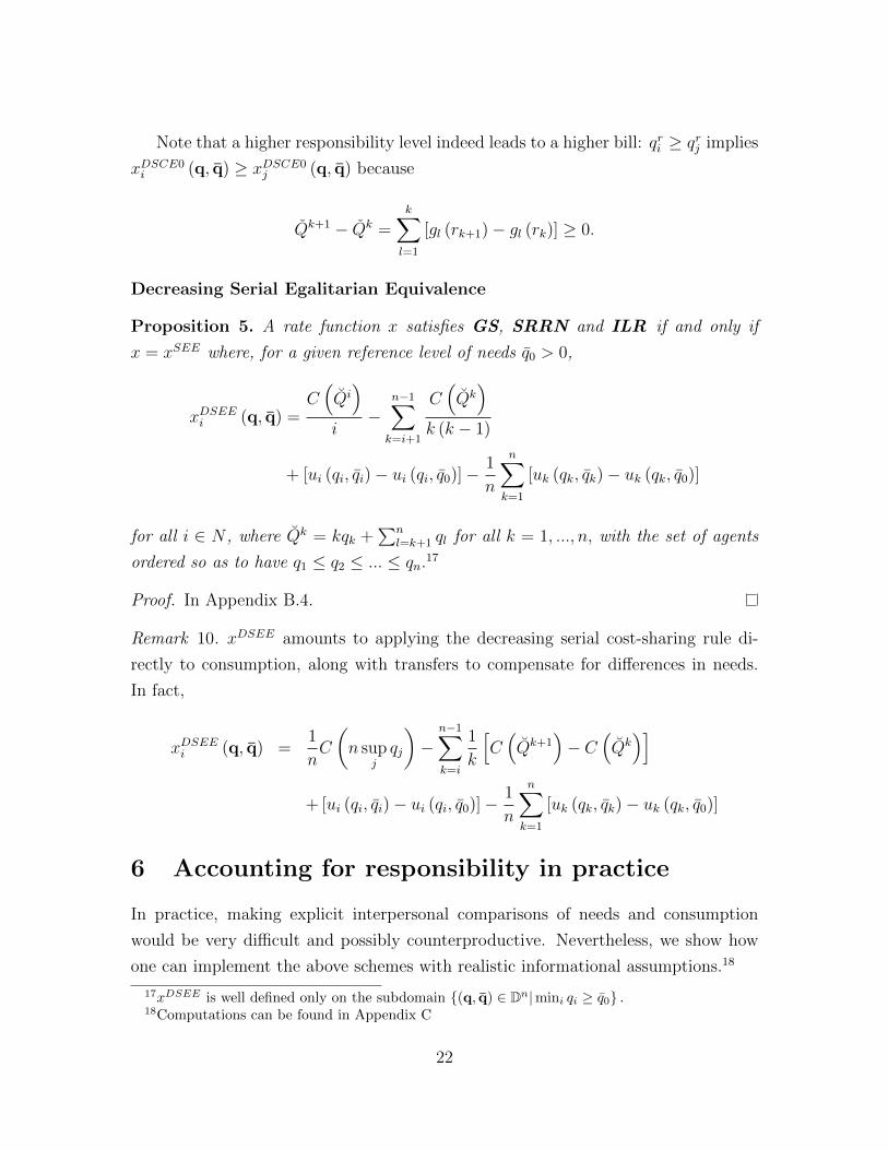
Proposition 5. A rate function x satisfies GS, SRRN and ILR if and only if

x = xSEE where, for a given reference level of needs q0 > 0,

xDSEEi (q, q) =C(Qi)

i−

n−1∑k=i+1

C(Qk)

k (k − 1)

+ [ui (qi, qi)− ui (qi, q0)]− 1

n

n∑k=1

[uk (qk, qk)− uk (qk, q0)]

for all i ∈ N , where Qk = kqk +∑n

l=k+1 ql for all k = 1, ..., n, with the set of agents

ordered so as to have q1 ≤ q2 ≤ ... ≤ qn.17

Proof. In Appendix B.4.

Remark 10. xDSEE amounts to applying the decreasing serial cost-sharing rule di-

rectly to consumption, along with transfers to compensate for differences in needs.

In fact,

xDSEEi (q, q) =1

nC

(n sup

jqj

)−

n−1∑k=i

1

k

[C(Qk+1

)− C

(Qk)]

+ [ui (qi, qi)− ui (qi, q0)]− 1

n

n∑k=1

[uk (qk, qk)− uk (qk, q0)]

6 Accounting for responsibility in practice

In practice, making explicit interpersonal comparisons of needs and consumption

would be very difficult and possibly counterproductive. Nevertheless, we show how

one can implement the above schemes with realistic informational assumptions.18

17xDSEE is well defined only on the subdomain {(q, q) ∈ Dn|mini qi ≥ q0} .18Computations can be found in Appendix C

22

6.1 Pricing using aggregate distributions

We now represent the population by a distribution. Assume that there is a finite

number of types in the needs dimension due to, say, household size, and let qs denote

the needs of a household of size s ∈ S. The planner does not know each individual’s

utility function, but has enough information to infer, us, the typical utility func-

tion of a household of type s ∈ S. Let ns (q) be the density of type-s households

with consumption level q and let Ns (q) be the associated cumulative distribution:

Ns (q) =∫ qz=0

ns (z) dz. Define n (q) =∑

s∈S ns (q) and N (q) =∑

s∈S Ns (q). We

slightly abuse notation and write r (q, s) instead of r (q, qs) whenever it is unambigu-

ous. Given the responsibility function r, define nrs (ρ) the density of type-s house-

holds with responsibility level ρ. Let N rs (ρ) be the associated cumulative distribution:

N rs (ρ) =

∫ ρz=0

nrs (z) dz and define N r (ρ) =∑

s∈S Nrs (ρ). We now define the following

continuous counterparts to the quantities Q, Q, Q and Q, respectively corresponding

to the SCE0, SEE, DSCE0 and DSEE schemes:

SCE0 : Q (ρ) =∑s∈S

[∫ +∞

0

gs (inf{ρ, z})nrs (z) dz

](9)

SEE : Q (q) =

∫ ∞0

inf{q, z}n (z) dz (10)

DSCE0 : Q (ρ) =

∫ ∞z=0

∑s∈S

gs (sup {ρ, z})nrs (z) dz (11)

DSEE : Q (q) =

∫ ∞z=0

sup{q, z}n (z) dz (12)

with gs (·) ≡ r−1 (·, qs).With this notation, the expressions for xSCE0, xSEE, xDSCE0, and xDSEE take the

23

following forms:

xSCE0 (ρ) =C(Q)

N+

∫ ρ

z=0

1

N −N r (z)C ′(Q (z)

) dQ (z)

dρdz (13)

xSEE (q, s) =C(N inf q)

N+

∫ q

z=0

C ′(Q (z)

)dz (14)

+ [us (q, qs)− u (qs, q0)]− 1

N

∑t∈S

∫ ∞z=0

[ut (z, qt)− ut (z, q0)]nt (z) dz

xDSCE0 (ρ) =1

NC(Qsup

)−∫ sup ~ρ

z=ρ

1

N r (z)C ′(Q (z)

) dQ (z)

dzdz (15)

xDSEE (q, s) = 1N

C (N sup q)−∫ supq

z=q

C ′(Q (z)

)dz (16)

+ [us (q, qs)− us (q, q0)]− 1

N

∑t∈S

∫ ∞z=0

[ut (z, qt)− ut (z, q0)]nt (z) dz

where Qsup = Q (sup ~ρ) with sup ~ρ the largest responsibility level in the population

and where N still denotes the total number of households.

6.2 Illustrative Examples

To illustrate, we now consider two specific forms for r. In the absolute responsibility

view, r (q, s) = q− qs, whereas in the relative responsibility view, r (q, s) = (q − qs) /qs.If s indeed denotes household size, the former holds households equally responsible

for consumption above needs regardless of their size. By contrast, the latter view

holds larger households less responsible than smaller households for an identical con-

sumption level above needs. In other words, needs also impact the way consumption

beyond them is considered.

Decreasing Returns to Scale : Quadratic Costs

Assume that costs are given by the following quadratic function: C (Q) = cQ2/2. Un-

der absolute responsibility, the serial conditional equality rule with zero responsibility

as a reference yields:

xSCE0 (q, s) =1

N

cQ2

2+ cQ

(q − qs −

Q− QN

). (17)

24

In words, users share the total cost equally and are rewarded or penalized for deviation

from the average responsibility level. These deviations are valued at marginal cost.

Under relative responsibility, however, marginal consumption is not priced equally

across household types. When responsibility is equally distributed across types, we

obtain the following expression:

xSCE0 (q, s) =1

N

cQ2

2+ cQ

Q

N

(q − qsqs− Q− Q

Q

). (18)

Again, xSCE0 charges everyone the average cost and prices deviations from the average

responsibility, but this time at the marginal cost of responsibility if needs were equal

to Q/N . Observe that if qs > Q/N consumption is priced at less than the marginal

cost while the consumption of households with lower-than-average needs (qs < Q/N)

is priced above marginal cost.19

The serial egalitarian equivalent solution takes on the following form:

xSEE (q, s) = cQ

(q − Q

2N

)(19)

+ [us (q, qs)− us (q, q0)]− 1

N

∑t∈S

∫ ∞z=0

[ut (z, qt)− ut (z, q0)]nt (z) dz.

Recall that the expression for xSEE is independent of the responsibility view (e.g.,

absolute or relative responsibility). However, payments now depend upon the utility

function. This calls for an observation. Suppose that a household’s type is simply its

size and that qs = q × s for some reference per-person level of needs, q. Given a con-

sumption level, q, it seems natural for the total bill to be lower for larger households.

For this to be the case, it must be that us (q, q × s) is decreasing in s, according to

Expression (19). This implies that household utility cannot be written as a simple

sum of the utility of its members, s×vq (q/s), where vq is some increasing and concave

function. Indeed, we would have:

d

ds[s× vq (q/s)] = vq

(qs

)− q

sv

′

q

(qs

)≥ 0, (20)

by the concavity of vq. Thus, one must refrain from modeling households as a sum of

19This is unlike the case of absolute responsibility above, where the marginal cost of responsibilitywas identical across households and equal to the marginal cost.

25

individual utility functions.20

Increasing Returns to Scale: Affine Costs

Assume costs are of the form C(Q) = F + cQ, with F, c ∈ R+. When responsibility

is measured by absolute responsibility, the decreasing serial conditional equality rule

yields:

xDSCE0 (q, s) =F + cQ

N+ c (q − qs) . (21)

In addition to splitting the fixed cost equally, xDSCE0 also splits the cost of the

population’s needs equally before charging users at marginal cost with a rebate equal

to the cost of meeting their needs.

Under the relative responsibility view, and if responsibility is identically dis-

tributed across types, we obtain:

xDSCE0 (q, s) =F

N+ c

1

qs/(Q/N

)q. (22)

As with absolute responsibility, xDSCE0 splits the fixed cost equally. No rebate is

granted, however, but consumption is priced at a rate that is inversely proportional

to one’s needs.

We now turn to xDSCEE:

xDSEE (q, s) =F

N+ cq (23)

+ [us (q, qs)− us (q, q0)]− 1

N

∑t∈S

∫ ∞z=0

[ut (z, qt)− ut (z, q0)]nt (z) dz

The cost-sharing portion of xDSEE splits the fixed cost equally and prices consump-

tion at marginal cost. Needs are completely absent from that component. However,

the redistributive portion of xDSEE ensures that heterogeneity in needs does not drive

20This is reminiscent of the Repugnant Conclusion in population ethics (Blackorby et al., 2005).The latter is a consequence of the pure utilitarian criterion, which deems any population alwaysworse off than a larger one sharing the same resources, even if the population size is such thatindividuals have barely enough to survive (see also Fleurbaey et al., 2014).

26

differences in welfare.

References

[1] American Water Works Association (2012), M1 Principles of Water Rates, Fees

and Charges, AWWA, 6th ed.

[2] Barr, T. and T. Ash (2015) “Sustainable Water Rate Design at the Western

Municipal Water District: The Art of Revenue Recovery, Water Use Efficiency,

and Customer Equity” In: Dinar, Ariel, Victor Pochat and Jose Albiac, Water

Pricing Experiences and Innovations, Springer, pp. 373-392.

[3] Barraque, B. and M. Montginoul (2015) “How to Integrate Social Objectives into

Water Pricing” In: Dinar, Ariel, Victor Pochat and Jose Albiac, Water Pricing

Experiences and Innovations, Springer, pp. 359-371.

[4] Bergantinos, G., J. Masso and A. Neme (2012), “The division problem with

voluntary participation,” Social Choice and Welfare, 38, 371-406.

[5] Billette de Villemeur, E. and J. Leroux (2011) ’Sharing the cost of global warm-

ing’, Scandinavian Journal of Economics, 113, 758-783.

[6] Billette de Villemeur, E. and J. Leroux (2016) ’Individualistic pricing cannot

handle variable demands: Budget balance requires acknowledging interdepen-

dence’, mimeo, available at http://ssrn.com/abstract=2816063

[7] Blackorby, C., Bossert, W., and D. Donaldson, Population Issues in Social Choice

Theory, Welfare Economics, and Ethics, Econometric Society Monographs, 2005.

[8] Bossert, W. (1995) ’Redistribution mechanisms based on individual characteris-

tics’, Math. Soc. Sci., 29 1-17.

[9] Bossert, W., and M. Fleurbaey (1996) ’Redistribution and Compensation’, Soc.

Choice Welfare, 13 343-355.

[10] Canadian Water and Wastewater Association (2015), “Rates and Full Cost Pric-

ing”, CWWA Members’ Briefing Book. Also available on the CWWA website:

http://www.cwwa.ca/policy e.asp Accessed Nov. 12th 2015.

27

[11] Cappelen, A. and B. Tungodden (2006) “A Liberal Egalitarian Paradox,” Eco-

nomics and Philosophy, 22, 393-408.

[12] David, M. (1959). “Welfare, income, and budget needs”, The Review of Eco-

nomics and Statistics, 41, 393-399.

[13] Dinar, A. and T. Ash (2015) “Water Budget Rate Structure: Experiences from

Several Urban Utilities in Southern California” In: Manuel Lago et al., Use of

Economic Incentives in Water Policy, Springer, pp. 147-170.

[14] Duclos, J. Y., and A. Araar (2007) Poverty and equity: measurement, policy and

estimation with DAD (Vol. 2). Springer Science & Business Media.

[15] Duclos, J. Y., Makdissi, P., and Q. Wodon (2005) “Poverty-Reducing Tax Re-

forms with Heterogeneous Agents”, Journal of Public Economic Theory, 7, 107-

116.

[16] Ebert, U. (1997). “Social welfare when needs differ: An axiomatic approach”,

Economica, 64, 233-244.

[17] Federation of Canadian Municipalities (2006), “Water and Sewer Rates:

Full Cost Recovery,” National Guide to Sustainable Municipal Infrastructure,

https://www.fcm.ca/Documents/reports/Infraguide/Water and Sewer Rates Full Cost Recovery EN.pdf

Accessed on Nov. 12th 2015.

[18] Fleurbaey, M. (1995) ’Equality and Responsibility’, European Economic Review,

39 683-689.

[19] Fleurbaey, M. (1995) “Three Solutions for the Compensation Problem”, Journal

of Economic Theory, 65(2), 505-521.

[20] Fleurbaey, M. (2008), Fairness, Responsibility and Welfare, Oxford University

Press.

[21] Fleurbaey, M., C. Hagnere, and A. Trannoy (2014) “Welfare comparisons of

income distributions and family size”, Journal of Mathematical Economics, 51,

12-27

[22] de Frutos, M. A. (1998) “Decreasing Serial Cost Sharing under Economies of

Scale,” Journal of Economic Theory, 79, 245-275.

28

[23] Garvy, G. (1954) “Functional and size distributions of income and their mean-

ing”, The American Economic Review, 44, 236-253.

[24] Gleick, P.H. (1996) “Basic Water Requirements for Human Activities: Meeting

Basic Needs”, Water International, 21, 83-92.

[25] Hicks, N. and P. Streeten (1979) “Indicators of development: the search for a

basic needs yardstick”, World Development, 7, 567-580.

[26] Konow, J. (2001) “Fair and square: the four sides of distributive justice,” Journal

of Economic Behavior & Organization, 46, 136-164.

[27] Manjunath, V. (2012) “When too little is as good as nothing at all: Rationing a

disposable good among satiable people with acceptance thresholds,” Games and

Economic Behavior, 74, 576-587.

[28] Massarutto, A. (2007) “Water Pricing and Full Cost Recovery of Water Services:

Economic Incentive or Instrument of Public Finance?”, Water Policy, 9, 591- 613.

[29] Mayshar, J., and S. Yitzhaki (1996) “Dalton-improving tax reform: When house-

holds differ in ability and needs”, Journal of Public Economics, 62, 399-412.

[30] Morgan, J. (1962) “The anatomy of income distribution”, The Review of Eco-

nomics and Statistics, 44, 270-283.

[31] Moulin, H. (2002) “Axiomatic cost and surplus sharing”, in Handbook of Social

Choice and Welfare, Chapter 6, 289-357.

[32] Moulin, H. (2003) Fair division and collective welfare, MIT Press.

[33] Moulin, H. and S. Shenker (1992) “Serial Cost Sharing,” Econometrica, 60, 1009-

1037.

[34] OECD (2010), Pricing Water Resources and Water and Sanitation Services,

OECD Studies on Water.

[35] Ooghe, E. (2015) “Partial Compensation/Responsibility,” Theory and Decision,

78, 305-317.

[36] Ooghe, E., and A. Peichl (2014) “Fair and Efficient Taxation under Partial Con-

trol,” The Economic Journal, doi 10.1111/ecoj.1216

29

[37] Pazner, E.A. and D. Schmeidler (1978) “Egalitarian Equivalent Allocations: A

New Concept of Economic Equity”, Quaterly Journal of Economics, 92(4), 671-

687.

[38] Streeten, A.M. (1979) “Basic Needs: Premises and Promises”, Journal of Policy

Modeling, 1, 136-146.

[39] Streeten, P. and S.J. Burki (1978) “Basic needs: some issues”, World Develop-

ment, 6, 411-421.

[40] Trannoy, A. (2003) “About the right weights of the social welfare function when

needs differ”, Economics Letters, 81, 383-387.

30

A Appendix: Section 4 Proofs

A.1 Proof of Theorem 2

Let r0 ∈ R+ be a reference responsibility level and (q0, q) ∈ P be such that,

r(q0i , qi

)= r0, for all i ∈ N. (24)

By UWRR,

ui(q0i , qi

)− xi

(q0,q

)= uj

(q0j , qj

)− xj

(q0,q

), for all i, j ∈ N. (25)

Hence, for all i ∈ N ,

xi(q0,q

)= ui

(q0i , qi

)− 1

n

∑j∈N

[uj(q0j , qj

)− xj

(q0,q

)], (26)

=C (Q0)

n+ ui

(q0i , qi

)− 1

n

∑j∈N

uj(q0j , qj

), (27)

where Q0 ≡∑

j∈N q0j .

Applying SR between profiles (q0, q) and (q, q) yields:

xi(q0, q)− xi(q, q) = ξi

(r0, C − C(Q)

). (28)

Hence, by symmetry of ξ,

xi(q, q) = xi(q0, q

)−C (Q0)− C

(Q)

n. (29)

Applying SR between profiles (q, q) and (q, q) yields:

xi(q, q)− xi(q, q) = ξi(r, C − C(Q)

). (30)

31

Thus,

xi(q, q) = ξi(r, C − C(Q)

)+ xi (q, q) (31)

= ξi(r, C − C(Q)

)+ xi

(q0, q

)−C (Q0)− C

(Q)

n(32)

= ξi(r, C − C(Q)

)+C(Q)

n+ ui

(q0i , qi

)− 1

n

∑j∈N

uj(q0j , qj

). (33)

A.2 Proof of Proposition 1

Let (q0, q) ∈ P and (q1, q) ∈ P be two profiles associated respectively with the

uniform responsibility profiles r0 = (r0, r0, ..., r0) and r1 = (r1, r1, ..., r1) with r1 6= r0.

Suppose that x satisfies UWUR so that it satisfies in particular UWRR for the

reference responsibility level r0. If it does also satisfy SR, it must be written as

xi (q, q) =C(Q)

n+ξi

(r, C − C(Q)

)+ui

(q0i , qi

)− 1

n

∑j∈N

uj(q0j , qj

), for all i ∈ N.

(34)

This says in particular that when q = q1, we have:

xi(q1, q

)=C(Q)

n+ξi

(r1, C − C(Q)

)+ui

(q0i , qi

)− 1

n

∑j∈N

uj(q0j , qj

), for all i ∈ N.

(35)

By symmetry of ξ, we have ξi(r1, C − C

(Q))

=[C (Q1)− C

(Q)]/n, for all i ∈ N

so that

xi(q1, q

)=C (Q1)

n+ ui

(q0i , qi

)− 1

n

∑j∈N

uj(q0j , qj

), for all i ∈ N. (36)

If x (q,q) satisfies UWRR for the reference responsibility level r1 (to which q1 is

associated), it must be the case that

ui(q1i , qi

)− xi

(q1, q

)= uj

(q1j , qj

)− xj

(q1, q

), for all i, j ∈ N. (37)

From the expression of xi (q1, q) established above, we must have

ui(q1i , qi

)− ui

(q0i , qi

)= uj

(q1j , qj

)− uj

(q0j , qj

), for all i, j ∈ N. (38)

32

This implies in turn that

ui(q1i , qi

)− ui

(q0i , qi

)=

1

n

∑j∈N

[uj(q1j , qj

)− uj

(q0j , qj

)], for all i ∈ N. (39)

This must be true for any responsibility level r0 and r1 and the associated profiles

(q0, q) ∈ P and (q1, q) ∈ P . Thus, by setting r1 = 0 and considering the associated

profile (q, q) ∈ P , we obtain that, for SR and UWUR to be compatible, the utility

function must be such that

ui(q0i , qi

)=

1

n

∑j∈N

uj(q0j , qj

)(40)

for all i ∈ N and for all profiles (q0, q) ∈ P such that

r(q0i , qi

)= r0, for all i ∈ N. (41)

Fix r0 and q and define, for all i ∈ N , q (r0, qi) = {q ∈ R+|r (q, qi) = r0}. By

continuity and strict monotonicity of r, q (r0, qi) is a singleton and (r0, qi) 7→ q (r0, qi)

defines a continuous function that is increasing in its first argument. Also, define

u0 = 1n

∑j∈N uj (q (r0, qj) , qj). It follows from Expression (40) that we must have

ui (q (r0, qi) , qi) = u0 for all i and all qi. Because u0 depends neither upon i, nor

uponqi, it must be that (qi, r0) 7→ ui (q (r0, qi) , qi) is a function of r0 only. Therefore,

for all r0, all i and all qi,

ui(q(r0, qi

), qi)

= v(r0)

(42)

for some function v on R. Because ui and q are both continuous and increasing in

their first argument, v is also a continuously increasing function.

Finally, let (qi, qi) ∈ D, evaluating the above expression at r0 = r (qi, qi), and

noticing that

q (r (qi, qi) , qi) = qi (43)

yields:

ui (qi, qi) = v (r (qi, qi)) . (44)

This in turn implies that the utility must be a transformation of the responsibility

function:

ui = u ≡ v ◦ r. (45)

33

Because v is a continuous and increasing function of R, we can write:

r = ρ ◦ u, (46)

with ρ = v−1, so that r is a transformation of the common utility functionu, as was

to be shown.

A.3 Proof of Theorem 3

Only if. Let x satisfy EWER and SR. Because EWER is more demanding than

UWUR, x must also satisfy UWUR . By Proposition 1, this can only occur if ui = u

for some utility function u and r = ρ ◦ u for some continuous and increasing function

ρ. Because UWUR is more demanding than UWRR, x must also satisfy UWRR.

By Theorem 2, x must be a Conditional Equivalent solution:

xCEi (q, q) =C(Q)

n+ ξi

(r, C − C(Q)

)+ u

(q0i , qi

)− 1

n

∑j∈N

u(q0j , qj

), (47)

where u is the common utility function and q0 is such that, for all i ∈ N , r (q0i , qi) = r0

for some reference responsibility level, r0. Moreover, it follows from r = ρ ◦ u that

u (q0i , qi) = ρ−1 (r0) for all i ∈ N . Hence,

xCEi (q, q) =C(Q)

n+ ξi

(r, C − C(Q)

), for all i ∈ N. (48)

If. We already know from Theorem 1 that xCE0 satisfies SR. Let (q, q) ∈ Dn

such that r (qi, qi) = r (qj, qj)for some i, j ∈ N . It follows from the symmetry of ξ

that

ξi(r, C − C(Q)

)= ξj

(r, C − C(Q)

). (49)

As a result,

xCE0i (q, q) = xCE0

j (q, q). (50)

Moreover, because r = ρ ◦ u for some continuous and increasing function ρ, we can

write u = ρ−1 ◦ r. Thus,

r (qi, qi) = r (qj, qj) =⇒ u (qi, qi) = u (qj, qj) , (51)

34

and ui = uj = u yields

ui (qi, qi)− xCE0i (q, q) = uj (qj, qj)− xCE0

j (q, q). (52)

Hence, xCE0 satisfies EWER.

A.4 Proof of Theorem 4

Let q0 ∈ R+ be a reference level of needs and denote by q0 = (q0, q0, ..., q0) ∈ Rn+

the associated reference vector. Let (q, q) ∈ Dn such that mini qi ≥ q0. By budget

balance and anonymity,

xi (q0, q0) =C(nq0)

n. (53)

By SRRN,

xi (q, q0)− xi (q0, q0) = ξi (r0, C − C (nq0)) for all i ∈ N, (54)

where r0,i = r (qi, q0) for all i.

Define q10 = (q1, q0, ..., q0). Applying GS between (q, q0) and (q, q1

0) yields, for all

j 6= 1:

u1 (q1, q1)− x11 − u1 (q1, q0) + x0

1 = uj (qj, q0)− x1j − uj (qj, q0) + x0

j (55)

where x0j = xj (q, q0) and x1

j = xj (q, q10) for all j ∈ N . This yields:

x0j − x1

j = u1 (q1, q1)− u1 (q1, q0) + x01 − x1

1, (56)

hence, by budget balance:x11 − x0

1 = n−1n

[u1 (q1, q1)− u1 (q1, q0)]

x1j − x0

j = − 1n

[u1 (q1, q1)− u1 (q1, q0)] ∀j 6= 1.(57)

Applying GS to profiles(q, qk0

)where qk0 = (q1, q2, ..., qk, q0, ..., q0), successively leads

to the following expression, for all iterations, k = 1, ..., n, and all agents 1 ≤ i ≤ k ≤

35

j ≤ n:

ui (qi, qi)− xki − ui (qi, qi) + xk−1i (58)

= uk (qk, qk)− xkk − uk (qk, q0) + xk−1k (59)

= uj (qj, q0)− xkj − uj (qj, q0) + xk−1j (60)

Hence, for all k = 1, ..., n, and all agents 1 ≤ i ≤ k ≤ j ≤ n:

xk−1i − xki (61)

= uk (qk, qk)− uk (qk, q0) + xk−1k − xkk (62)

= xk−1j − xkj (63)

By budget balance,∑

j

(xkj − xk−1

j

)= 0, yielding:

xkk − xk−1k =

n− 1

n[uk (qk, qk)− uk (qk, q0)] (64)

xkj − xk−1j = − 1

n[uk (qk, qk)− uk (qk, q0)] for all j 6= k. (65)

Summing up over all iterations k yields the following:

xn1 − x01 =

n∑k>1

(xk1 − xk−1

1

)+ x1

1 − x01 (66)

= − 1

n

n∑j>1

[uj (qj, qj)− uj (qj, q0)] +

(1− 1

n

)[u1 (q1; q1)− u1 (q1; q0)](67)

= [u1 (q1, q1)− u1 (q1, q0)]− 1

n

n∑j=1

[uj (qj, qj)− uj (qj; q0)] (68)

Likewise, for all i ∈ N :

xni − x0i = [ui (qi, qi)− ui (qi, q0)]− 1

n

n∑j=1

[uj (qj, qj)− uj (qj, q0)] (69)

Finally, upon noticing that xni = x (q, q) and x0i = xi (q, q0), Expression (54)

36

yields:

xi (q, q) = ξi (r0, C − C (nq0)) + xi (q0, q0) (70)

+ [ui (qi, qi)− ui (qi, q0)]− 1

n

n∑j=1

[uj (qj, qj)− uj (qj, q0)] . (71)

Expression (53) yields the result.

A.5 Proof of tightness of the characterization of EE by SRRN

and GS

Let xEE be the egalitarian equivalent solution defined relative to reference needs level

q0 ≥ 0 and consider a profile (q, q1) ∈ Dn such that q1 = (q1, q1, ..., q1) with q1 > q0.

Then:

xEEi (q, q1)− xEEi (q1, q1) =C(nq0)

n+ ξi (r0, C − C (nq0)) (72)

+ [ui (qi, q1)− ui (qi, q0)]− 1

n

n∑k=1

[uk (qk, q1)− uk (qk, q0)]

−(C(nq0)

n+ ξi (r0, C − C (nq0)) ...

...+ [ui (q1, q1)− ui (q1, q0)]− 1

n

n∑k=1

[uk (q1, q1)− uk (q1, q0)]

)

where r0 ≡ (r (q1, q0) , r (q1, q0) , ..., r (q1, q0)) ∈ Rn+. Hence, upon noticing that ξi (r0, C − C (nq0)) =

1n

(C (nq1)− C (nq0)), Expression (72) simplifies into:

xEEi (q, q1)− xEEi (q1, q1) = ξi (r0, C − C (nq0))− 1

n(C (nq1)− C (nq0)) (73)

+ (ui (qi, q1)− ui (q1, q1)− [ui (qi, q0)− ui (q1, q0)])

− 1

n

n∑k=1

(uk (qk, q1)− uk (qk, q0)− [uk (q1, q1)− uk (q1, q0)])

The above expression reveals that xEEi (q, q1)−xEEi (q1, q1) depends on ui, hence

cannot be driven only by the cost sharing function ξ. In other words, it cannot be

37

the case that:

xEEi (q, q1)− xEEi (q1, q1) = ξi (r1, C − C (nq1)) ,

as required by SRUN.

B Section 5 Proofs

B.1 Proof of Proposition 2

Let (qq) ∈ Dn+. By UWMC,

xi(q, q) = xj(q, q) for all i, j ∈ N (74)

=⇒ xi(q, q) =C(Q)

nfor all i ∈ N (75)

by budget balance. Without any loss of generality, assume that r1 ≤ r2 ≤ ... ≤ rn.

Let fi : w 7→ r (w, qi) map consumption to individual responsibility for agent i. By

construction, fi is monotonic and strictly increasing. Its inverse, gi : v 7→ f−1i (v) is

well defined and is also monotonic and strictly increasing. Note that gi (ri) = qi for

all i ∈ N .

Define the following profile:

q1= (q1, g2 (r1) , ..., gi (r1) , ..., gn (r1)) . (76)

Note that, by construction (q1, q) is such that r1i = r1 for all i ∈ N. Applying SR

with profile (q1, q) yields:

xi(q1, q

)− xi (q, q) = ξi

(r1, C − C

(Q)), (77)

By symmetry of ξ and because all r1i are identical, we have:

ξi(r1, C − C

(Q))

=1

n

[C(Q1)− C

(Q)], (78)

where

Q1 =n∑i=1

q1i =

n∑i=1

gi (r1) . (79)

38

Similarly, let

q2= (q1, q2, g3 (r2) , ..., gi (r2) , ..., gn (r2)) . (80)

Again by construction (q2, q) is such that r2i = r2 for all i = 2, ..., n. Applying now

SR with profile (q2, q) yields:

xi(q2, q

)− xi (q, q) = ξi

(r2, C − C

(Q)). (81)

As before, the symmetry of ξ yields:

ξi(r2, C − C

(Q))

= ξj(r2, C − C

(Q)), (82)

for all i, j ≥ 2. Moreover, because r1 ≤ r2, applying IHR between profiles (q1, q)

and (q2, q) yields that agent 1’s contribution is the same under both profiles:

ξ1

(r1, C − C

(Q))

= ξ1

(r2, C − C

(Q))

=1

n

[C(Q1)− C

(Q)], (83)

Thus, agents 2, ..., n share the remaining cost equally:

ξi(r2, C − C

(Q))

=1

n− 1

[C(Q2)− C

(Q)− 1

n

[C(Q1)− C(Q)

]](84)

=1

n− 1

[C(Q2)− C

(Q1)]

+1

n

[C(Q1)− C(Q)

](85)

for all i ≥ 2, where

Q2 =n∑i=1

q2i = q1 +

n∑i=2

gi (r2) ≥ Q1. (86)

Alternatively,

ξi(r2, C − C

(Q))− ξi

(r1, C − C

(Q))

=1

n− 1

[C(Q2)− C

(Q1)]

all i ≥ 2.

Similarly, for all k ≥ 2, we define

qk = (q1, q2, ..., qk, gk+1 (rk) , ..., gn (rk)) , (87)

39

and obtain by SR that

xi(qk, q

)− xi (q, q) = ξi

(rk, C − C

(Q)), (88)

for all i ∈ N . It follows thatξi(rk, C − C

(Q))− ξi

(rk−1, C − C

(Q))

= 0 for all i < k, and

ξi(rk, C − C

(Q))− ξi

(rk−1, C − C

(Q))

= 1n−k+1

[C(Qk)− C

(Qk−1

)]for all i ≥ k,

(89)

with

Qk =n∑i=1

qki =k−1∑i=1

qi +n∑i=k

gi (rk) . (90)

Observe that

Qk+1 − Qk =n∑

i=k+1

[gi (rk+1)− gi (rk)] ≥ 0 (91)

by monotonicity of the gi’s. It follows that xi+1

(qk, q

)≥ xi

(qk, q

), for all i ∈ N , so

that agents with a higher ri pay a higher bill for all k.

To sum up, upon observing that rn = r (as associated to profile (q, q)), we obtain

xk (q, q)− xk (q, q) =k∑i=1

1

n− i+ 1

[C(Qi)− C

(Qi−1

)](92)

where Q0 = Q. Finally,

xk (q, q) =1

nC(Q)

+k∑i=1

1

n− i+ 1

[C(Qi)− C

(Qi−1

)](93)

=

[1

n− 1

n

]C(Q0)

+

[1

n− 1

n− 1

]C(Q1)

+

[1

n− 1− 1

n− 2

]C(Q2)

(94)

+...+

[1

n− i+ 1− 1

n− i

]C(Qi)

+ ...+1

n− k + 1C(Qk)

xk (q, q) =C(Qk)

(n− k + 1)−

k−1∑i=1

C(Qi)

(n− i) (n− i+ 1)=C(Qk)

n− k−

k∑i=1

C(Qi)

(n− i) (n− i+ 1)(95)

40

with

Qk =k−1∑i=1

qi +n∑i=k

gi (rk) . (96)

B.2 Proof of Proposition 3

Let (qq) ∈ Dn+. Let q0 ∈ R+ be a reference level of needs and denote by q0 =

(q0, q0, ..., q0) ∈ Rn+ the associated reference vector. Let (q, q) ∈ Dn such that

mini qi ≥ q0. By budget balance and anonymity,

xi (q0, q0) =C(nq0)

nfor all i ∈ N. (97)

Without loss of generality, assume that q1 ≤ q2 ≤ ... ≤ qn, so that r0,1 ≤ r0,2 ≤ ... ≤r0,n, where r0,i = r (qi, q0) for all i ∈ N .

For all k ∈ N , define

qk = (q1, q2, ..., qk−1, qk, ..., qk) . (98)

Notice that q1 = (q1, q1, ..., q1); hence, by anonymity,

xi(q1, q0

)=C (nq1)

n(99)

and

xi(q1, q0

)− xi (q0, q0) =

1

n[C (nq1)− C (nq0)] (100)

for all i ∈ N .

Similarly, for k ≥ 2, SRRN yields

xi(qk, q0

)− xi (q0, q0) = ξi

(rk0, C − C (nq0)

)(101)

and

xi(qk−1, q0

)− xi (q0, q0) = ξi

(rk−1

0 , C − C (nq0))

(102)

for all i ∈ N , with rk0,i = r(qki , q0

)and rk−1

0,i = r(qk−1i , q0

). Therefore, by subtraction,

xi(qk, q0

)− xi

(qk−1, q0

)= ξi

(rk0, C − C (nq0)

)− ξi

(rk−1

0 , C − C (nq0))

(103)

41

for all i ∈ N . Summing up over all agents, we find:

n∑i=1

[xi(qk, q0

)− xi

(qk−1, q0

)]= C

(Qk)− C

(Qk−1

), (104)

where Qk−1 =∑n

l=1 qk−1l =

∑k−1l=1 ql + (n− k + 1) qk−1 and Qk =

∑nl=1 q

kl =

∑kl=1 ql +

(n− k) qk.

Observe that if i < j then rk−10,i ≤ rk−1

0,j and rk0,i ≤ rk0,j. Moreover for all 1 ≤ i ≤k − 1, qk−1

i = qki = qi, and rk−10,i = rk0,i = r (qi, q0). Therefore, by IHR,

xi(qk, q0

)− xi

(qk−1, q0

)= 0, (105)

for all 1 ≤ i ≤ k − 1. It follows that the previous summation can truncated from

below:n∑i=k

[xi(qk, q0

)− xi

(qk−1, q0

)]= C

(Qk)− C

(Qk−1

). (106)

Moreover, for all i, j ≥ k, we have qk−1i = qk−1

j = qk−1 and qki = qkj = qk. Therefore,

by anonymity,

xi(qk−1, q0

)= xj

(qk−1, q0

)and xi

(qk, q0

)= xj

(qk, q0

)(107)

for all i, j ≥ k.

Hence,

xi(qk, q0

)− xi

(qk−1, q0

)=

1

n− k + 1

[C(Qk)− C

(Qk−1

)](108)

for all i ≥ k, with the convention that Q0 = nq0.

Finally, upon observing that qn = q, it follows by summation that

xi (q, q0)− xi (q0, q0) =i∑

k=1

1

n− k + 1

[C(Qk)− C

(Qk−1

)]; (109)

i.e., substituting according to Expression (97):

xi (q, q0) =C(nq0)

n+

i∑k=1

1

n− k + 1

[C(Qk)− C

(Qk−1

)](110)

42

We now work along the needs dimension. Define q10 = (q1, q0, ..., q0). Applying

GS between (q, q0) and (q, q10) yields, for all j 6= 1:

u (q1, q1)− x11 − u (q1, q0) + x0

1 = u (qj, q0)− x1j − u (qj, q0) + x0

j , (111)

where x0j = xj (q, q0) and x1

j = xj (q, q10) for all j ∈ N . This yields

x0j − x1

j = u (q1, q1)− u (q1, q0) + x01 − x1

1. (112)

Since total consumption is unchanged, we have, by budget balance

x11 − x0

1 =n− 1

n[u (q1, q1)− u (q1, q0)] , and (113)

x1j − x0

j = − 1

n[u (q1, q1)− u (q1, q0)] . (114)

for all j 6= 1.

Iterating and applying GS to profiles(q, qk0

)where qk0 = (q1, q2, ..., qk, q0, ..., q0),

successively leads to the following expression, for all iterations, k = 1, ..., n, and all

1 ≤ i ≤ k ≤ j ≤ n:

u (qi, qi)− xki − u (qi, qi) + xk−1i = u (qk, qk)− xkk − u (qk, q0) + xk−1

k (115)

= u (qj, q0)− xkj − u (qj, q0) + xk−1j (116)

where xk−1j = xj

(q, qk−1

0

)and xkj = xj

(q, qk0

). Hence, for all k = 1, ..., n, and all

1 ≤ i ≤ k ≤ j ≤ n:

xk−1i − xki = u (qk, qk)− u (qk, q0) + xk−1

k − xkk (117)

= xk−1j − xkj (118)

Since total consumption does not change from(q, qk−1

0

)to(q, qk0

), but only needs,

budget balance implies∑

j

(xkj − xk−1

j

)= 0. Therefore,

xkj − xk−1j = − 1

n[u (qk, qk)− u (qk, q0)] for all j 6= k, and (119)

xkk − xk−1k =

n− 1

n[u (qk, qk)− u (qk, q0)] (120)

43

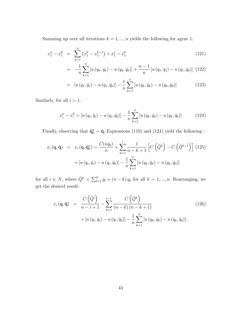
Summing up over all iterations k = 1, ..., n yields the following for agent 1:

xn1 − x01 =

n∑k>1

(xk1 − xk−1

1

)+ x1

1 − x01 (121)

= − 1

n

n∑k>1

[u (qk, qk)− u (qk, q0)] +n− 1

n[u (q1, q1)− u (q1, q0)] (122)

= [u (q1, q1)− u (q1, q0)]− 1

n

n∑k=1

[u (qk, qk)− u (qk, q0)] (123)

Similarly, for all i > 1:

xni − x0i = [u (qi, qi)− u (qi, q0)]− 1

n

n∑k=1

[u (qk, qk)− u (qk, q0)] (124)

Finally, observing that qn0 = q, Expressions (110) and (124) yield the following :

xi (q, q) = xi (q, qn0 ) =

C(nq0)

n+

i∑k=1

1

n− k + 1

[C(Qk)− C

(Qk−1

)](125)

+ [u (qi, qi)− u (qi, q0)]− 1

n

n∑k=1

[u (qk, qk)− u (qk, q0)]

for all i ∈ N , where Qk =∑k

l=1 ql + (n− k) qk for all k = 1, ..., n. Rearranging, we

get the desired result:

xi (q, q) =C(Qi)

n− i+ 1−

i−1∑k=1

C(Qk)

(n− k) (n− k + 1)(126)

+ [u (qi, qi)− u (qi, q0)]− 1

n

n∑k=1

[u (qk, qk)− u (qk, q0)] .

44

B.3 Proof of Proposition 4

The proof follows the same blueprint as that of Proposition 2. Let (qq) ∈ Dn+. By

UWMC,

xi(q, q) = xj(q, q) for all i, j ∈ N (127)

=⇒ xi(q, q) =C(Q)

n(128)

Without loss of generality, assume that r1 ≤ r2 ≤ ... ≤ rn. Let fi : w 7→ r (w, qi)

map consumption to the individual responsibility for agent i. By construction, fi

is monotonic and strictly increasing. Its inverse, gi : v 7→ f−1i (v) is well defined,

monotonic and strictly increasing. Note that gi (ri) = qi for all i ∈ N .

Define the following profile:

qn= (g1 (rn) , ..., gi (rn) , ..., gn−1 (rn) , qn) . (129)

Note that, by construction (qn, q) is such that

rni = rn, (130)

for all i ∈ N.

Applying SR to profile (qn, q) yields:

xi(qn, q)− xi(q, q) = ξi(r

n, C − C(Q)), (131)

where ξi(r, C − C(Q)) is symmetric in r. Since all rni ’s are identical, we have

ξi(rn, C − C(Q)) =

1

n

[C(Qn)− C(Q)

], (132)

where

Qn =n∑i=1

qni =n∑i=1

gi (rn) . (133)

This gives

xi(qn, q) =

1

nC(Qn). (134)

45

Similarly, let

qn−1= (g1 (rn−1) , ..., gi (rn−1) , ..., gn−2 (rn−1) , qn−1, qn) . (135)

Again, by construction (qn−1, q) is such that

rn−1i = rn−1, (136)

for all i = 1, ..., n− 1.

Applying now SR to profile (qn−1, q) yields:

xi(qn−1, q)− xi(q, q) = ξi(r

n−1, C − C(Q)), (137)

where ξi(r, C − C(Q)) is symmetric in r, therefore

ξi(rn−1, C − C(Q)) = ξj(r

n−1, C − C(Q)) (138)

for all i, j ≤ n− 1. In words, agents 1, ..., n− 1 are assigned the same cost share.

Moreover, by assumption rn ≥ rn−1. Thus, applying ILR between profiles (qn, q) and

(qn−1, q) yields that agent n’s contribution is the same under both profiles:

ξn(rn−1, C − C(Q)) = ξn(rn, C − C(Q)) =1

n

[C(Qn)− C(Q)

], (139)

Thus, agents 1, ..., n− 1 share the remaining cost equally:

ξi(rn−1, C − C(Q)) =

1

n− 1

[C(Qn−1

)− C

(Q)− 1

n

[C(Qn)− C(Q)

]](140)

=1

n

[C(Qn)− C(Q)

]− 1

n− 1

[C(Qn)− C

(Qn−1

)](141)

for all i ≤ n− 1, where

Qn−1 =n∑i=1

qn−1i =

n−1∑i=1

gi (rn−1) + qn ≤ Qn. (142)

Alternatively,

ξi(rn−1, C − C(Q))− ξi(rn, C − C(Q)) = − 1

n− 1

[C(Qn)− C

(Qn−1

)](143)

46

all i ≤ n− 1.

Similarly, for all k ≤ n− 1, we define

qk = (g1 (rk) , ..., gk−1 (rk) , qk, ..., qn−1, qn) (144)

and obtain by SR that

xi(qk, q)− xi(q, q) = ξi(r

k, C − C(Q)), (145)

for all i ∈ N . It follows that

ξi(rk, C − C(Q))− ξi(rk+1, C − C(Q)) = 0 for all i > k, and (146)

ξi(rk, C − C(Q))− ξi(rk+1, C − C(Q)) = −1

k

[C(Qk+1

)− C

(Qk)]

for all i ≤ k,(147)

with

Qk =n∑i=1

qki =k∑i=1

gi (rk) +n∑

i=k+1

qi. (148)

Observe that

Qk+1 − Qk =k∑i=1

[gi (rk+1)− gi (rk)] ≥ 0 (149)

by monotonicity of the gi’s. It follows that xi+1

(qk, q

)≥ xi

(qk, q

), all i ∈ N. It

follows from our initial ordering of the agents that agents with a higher ri pay a higher

bill for all k.

To sum up, upon observing that r1 = r (as associated to (q, q)), we obtain

xk (q, q)− xk (q, q) =1

n

[C(Qn)− C(Q)

]−

n−1∑i=k

1

i

[C(Qi+1

)− C

(Qi)]

(150)

47

where Q1 = Q. Finally,

xk (q, q) =1

nC (Qn)−

n−1∑i=k

1

i

[C(Qi+1

)− C

(Qi)]

(151)

=

[1

n− 1

n− 1

]C(Qn)

+

[1

n− 1− 1

n− 2

]C(Qn−1

)+

[1

n− 2− 1

n− 3

]C(Qn−2

)(152)

+...+

[1

i− 1

i− 1

]C(Qi)

+ ...+1

kC(Qk)

xk (q, q) =C(Qk)

k − 1−

n∑i=k

C(Qi)

i (i− 1)=C(Qk)

k−

n∑i=k+1

C(Qi)

i (i− 1)(153)

with

Qk =k∑i=1

gi (rk) +n∑

i=k+1

qi. (154)

B.4 Proof of Proposition 5

The proof follows the same blueprint as that of Proposition 3. Let q0 ∈ R+ be

a reference level of needs and denote by q0 = (q0, q0, ..., q0) ∈ Rn+ the associated

reference vector. Let (q, q) ∈ Dn such that mini qi ≥ q0. By budget balance and

anonymity,

xi (q0, q0) =C(nq0)

n. (155)

Without loss of generality, assume that q1 ≤ q2 ≤ ... ≤ qn, so that r0,1 ≤ r0,2 ≤ ... ≤r0,n, where r0,i = r (qi, q0) for all i ∈ N .

Define

qk = (qk, ..., qk, qk+1, ..., qn−1, qn) (156)

for all k = 1...n.

Notice that qn = (qn, qn, ..., qn); hence, by anonymity, xi (qn, q0) = C (nqn) /n so that

xi (qn, q0)− xi (q0, q0) =

1

n[C (nqn)− C (nq0)] (157)

for all i ∈ N.Similarly, for k ≤ n− 1, SRRN yields

xi(qk+1, q0

)− xi (q0, q0) = ξi

(rk+1

0 , C − C (nq0))

(158)

48

and

xi(qk, q0

)− xi (q0, q0) = ξi

(rk0, C − C (nq0)

)(159)

with rk+10,i = r

(qk+1i , q0

)and rk0,i = r

(qki , q0

). Therefore, by subtraction,

xi(qk, q0

)− xi

(qk+1, q0

)= ξi

(rk0, C − C (nq0)

)− ξi

(rk+1

0 , C − C (nq0))

(160)

for all i ∈ N and summing up over all agents, we find

n∑i=1

[xi(qk, q0

)− xi

(qk+1, q0

)]= −

[C(Qk+1

)− C

(Qk)], (161)

where Qk =∑n

l=1 qkl = kqk +

∑nl=k+1 ql and Qk+1 =

∑nl=1 q

k+1l = (k − 1) qk+1 +∑n

l=k+1 ql.

Observe that if i < j then rk0,i ≤ rk0,j and rk+10,i ≤ rk+1

0,j . Moreover for all k+ 1 ≤ i ≤ n,

qki = qk+1i = qi, and rk0,i = rk+1

0,i = r (qi, q0). Therefore, by ILR,

xi(qk, q0

)− xi

(qk+1, q0

)= 0, (162)

for all k + 1 ≤ i ≤ n. It follows that the previous summation can truncated from

above:k∑i=1

[xi(qk, q0

)− xi

(qk+1, q0

)]= −

[C(Qk+1

)− C

(Qk)], (163)

where 1 ≤ k ≤ n− 1.

Moreover, for all i, j ≤ k, we have qk+1i = qk+1

j = qk+1 and qki = qkj = qk . Therefore,

by anonymity,

xi(qk+1, q0

)= xj

(qk+1, q0

)(164)

all i, j ≤ k, and

xi(qk, q0

)= xj

(qk, q0

). (165)

Hence,

xi(qk, q0

)− xi

(qk−1, q0

)= −1

k

[C(Qk+1

)− C

(Qk)]

(166)

49

all i ≤ k.

Finally, upon observing that q1 = q, it follows by summation that

xi (q, q0)−xi (q0, q0) =1

n[C (nqn)− C (nq0)]−

n−1∑k=i

1

k

[C(Qk+1

)− C

(Qk)]

, (167)

so that

xi (q, q0) =1

nC (nqn)−

n−1∑k=i

1

k

[C(Qk+1

)− C

(Qk)]

. (168)

Define q10 = (q1, q0, ..., q0). Applying GS between (q, q0) and (q, q1

0) yields, for all

j 6= 1:

u (q1, q1)− x11 − u (q1, q0) + x0

1 = u (qj, q0)− x1j − u (qj, q0) + x0

j

where x0j = xj (q, q0) and x1

j = xj (q, q10) for all j ∈ N . This yields:

x0j − x1

j = u (q1, q1)− u (q1, q0) + x01 − x1

1. (169)

Becuase total consumption is unchanged, we have by budget balance:

x11 − x0

1 =n− 1

n[u (q1, q1)− u (q1, q0)] (170)

x1j − x0

j = − 1

n[u (q1, q1)− u (q1, q0)] (171)

all j 6= 1.

Iterating and applying GS to profiles(q, qk0

)where qk0 = (q1, q2, ..., qk, q0, ..., q0),

successively leads to the following expression, for all iterations, k = 1, ..., n, and all

agents 1 ≤ i ≤ k ≤ j ≤ n:

u (qi, qi)− xki − u (qi, qi) + xk−1i = u (qk, qk)− xkk − u (qk, q0) + xk−1

k (172)

= u (qj, q0)− xkj − u (qj, q0) + xk−1j (173)

Hence, for all k = 1, ..., n, and all agents 1 ≤ i ≤ k ≤ j ≤ n:

xk−1i − xki = u (qk, qk)− u (qk, q0) + xk−1

k − xkk (174)

= xk−1j − xkj (175)

50

Because total consumption does not change from(q, qk−1

0

)to(q, qk0

), but only needs,

budget balance implies∑

j

(xkj − xk−1

j

)= 0. Therefore,

xkj − xk−1j = − 1

n[u (qk, qk)− u (qk, q0)] for all j 6= k (176)

xkk − xk−1k =

n− 1

n[u (qk, qk)− u (qk, q0)] (177)

Summing up over all iterations k = 1, ..., n yields the following for agent 1:

xn1 − x01 =

n∑k>1

(xk1 − xk−1

1

)+ x1

1 − x01 (178)

= − 1

n

n∑k>1

[u (qk, qk)− u (qk, q0)] +n− 1

n[u (q1, q1)− u (q1, q0)] (179)

= [u (q1, q1)− u (q1, q0)]− 1

n

n∑k=1

[u (qk, qk)− u (qk, q0)] (180)

Similarly, for all i > 1:

xni − x0i = [u (qi, qi)− u (qi, q0)]− 1

n

n∑k=1

[u (qk, qk)− u (qk, q0)] (181)

Finally, observing that qn0 = q yields the following:

xi (q, q) = xi (q, qn0 ) =

1

nC(Qn)−

n−1∑k=i

1

k

[C(Qk+1

)− C

(Qk)]

(182)

+ [u (qi, qi)− u (qi, q0)]− 1

n

n∑k=1

[u (qk, qk)− u (qk, q0)]

Rearranging, we obtain the desired result:

xi (q, q) =C(Qi)

i−

n−1∑k=i+1

C(Qk)

k (k − 1)(183)

+ [u (qi, qi)− u (qi, q0)]− 1

n

n∑k=1

[u (qk, qk)− u (qk, q0)]

where Qk = kqk +∑n

l=k+1 ql for all k = 1, ..., n.

51

C Supplementary material: Calculations not in-

tended for publication

For the upcoming calculations, it will be convenient to introduce theNs =∫∞z=0

ns (z) dz

is the total number of type-s households.

C.1 Decreasing Returns to Scale: Quadratic Costs

SCE0 with absolute responsibility

Recall that

xSCE0 (ρ) =C(Q)

N+

∫ ρ

z=0

1

N −N r (z)C ′(Q (z)

) dQ (z)

dρdz, (184)

where

Q (ρ) =∑s∈S

[∫ +∞

0

inf{gs (z) , gs (ρ)}nrs (z) dz

]. (185)

Under the absolute responsibility view,

dQ (ρ)

dρ=∑s∈S

(Ns −N rs (ρ)) g′s (ρ) = N −N r (ρ) , (186)

with the second equality following from the fact that gs (ρ) ≡ qs + ρ. Hence,

xSCE0 (ρ) =C(Q)

N+

∫ ρ

z=0

C ′(Q (z)

)dz, (187)

with

Qs (ρ) =

∫ ρ

0

(qs + z)nrs (z) dz + (Ns −N rs (ρ)) (qs + ρ) (188)

= qsNs +

∫ ρ

0

znrs (z) dz + (Ns −N rs (ρ)) ρ (189)

= qsNs +

∫ +∞

0

min{z, ρ}nrs (z) dz, (190)

52

so that

Q (ρ) = Q+

∫ +∞

0

min{z, ρ}nr (z) dz (191)

= Q+

∫ r

0

znr (z) dz + (N −N r (ρ)) ρ (192)

Consider the case where C (Q) = c2Q2. It follows that C ′ (Q) = cQ, so that

xSCE0 (ρ) =cQ2

2N+ c

∫ ρ

z=0

Q (z) dz (193)

=cQ2

2N+ c

∫ ρ

z=0

[Q+

∫ +∞

y=0

min{y, z}nr (y) dy

]dz (194)

=cQ2

2N+ cQρ+ c

∫ +∞

y=0

nr (y)

∫ ρ

z=0

min{y, z}dzdy (195)

=cQ2

2N+ cQρ+ c

∫ +∞

y=0

nr (y)

[∫ y

z=0

zdz +

∫ ρ

z=y

ydz

]dy (196)

=cQ2

2N+ cQρ+ c

∫ +∞

y=0

nr (y)

[y2

2+ y (ρ− y)

]dy, (197)

=cQ2

2N+ cQρ+ c

∫ +∞

y=0

nr (y)

[yρ− y2

2

]dy. (198)

Upon noticing that Q+∫ +∞y=0

nr (y) ydy = Q under absolute responsibility, the above

expression rewrites as follows:

xSCE0 (ρ) =cQ2

2N− c

∫ +∞

y=0

nr (y)y2

2dy + cQρ. (199)

By budget balance,

cQ2

2=

∫ +∞

z=0

xSCE0 (z)nr (z) dz (200)

= N

[cQ2

2N− c

∫ +∞

y=0

nr (y)y2

2dy

]+ cQ

∫ +∞

z=0

znr(z)dz (201)

= N

[cQ2

2N− c

∫ +∞

y=0

nr (y)y2

2dy

]+ cQ

(Q− Q

). (202)

53

Thus,cQ2

2N− c

∫ +∞

y=0

nr (y)y2

2dy =

1

N

(cQ2

2− cQ

(Q− Q

)). (203)

Finally, it follows that

xSCE0 (ρ) =1

N

[cQ

(Q− Q

2

)]+ cQρ (204)

=1

N

cQ2

2+ cQ

(ρ− Q− Q

N

)(205)

Upon recalling that ρ = q − qs under absolute responsibility, we obtain the result:

xSCE0 (q, s) =1

N

cQ2

2+ cQ

(q − qs −

Q− QN

). (206)

SCE0 with relative responsibility

Recall that

xSCE (ρ) =C(Q)

N+

∫ ρ

z=0

1

N −N r (z)C ′(Q (z)

) dQ (z)

dzdz, (207)

where, from Expressions (191) and (192), we can write:

Q (ρ) =∑s∈S

[∫ +∞

0

gs (inf{z, ρ})nrs (z) dz

](208)

=∑s∈S

[∫ ρ

0

gs (z)nrs (z) dz + (Ns −N rs (ρ)) gs (ρ)

](209)

Under relative responsibility, ρ = (q − qs) /qs so that gs (ρ) = qs (1 + ρ). It follows

that g′s (ρ) = qs and

dQs (ρ)

dρ= (Ns −N r

s (ρ)) g′s (ρ) = (Ns −N rs (ρ)) qs. (210)

We now make an additional assumption. Namely, we posit that responsibility is

evenly spread across types, so that its distribution is independent of needs, qs:

N rs (ρ) = α (ρ)Ns ∀s ∈ S, (211)

54

for some increasing function α : R+ → [0, 1] which we take to be differentiable. This

yields:dQ (ρ)

dρ= (1− α (ρ)) Q. (212)

Also, because N −N r (ρ) = (1− α (ρ))N , we have

1

N −N r (ρ)

dQ (ρ)

dρ=Q

N, (213)

so that xSCE0 (ρ) simplifies to

xSCE0 (ρ) =C(Q)

N+Q

N

∫ ρ

z=0

C ′(Q (z)

)dz. (214)

Upon noticing that nrs (ρ) = α′ (ρ)Ns we get

Q (ρ) =

∫ +∞

0

∑s∈S

inf{gs (z) , gs (ρ)}Nsα′ (z) dz (215)

=

∫ +∞

0

inf{∑s∈S

Nsgs (z) ,∑s∈S

Nsgs (ρ)}α′ (z) dz (216)

where the summation sign enters the minimum operator because, for any s ∈ S,

gs (z) ≤ gs (ρ) if and only if z ≤ ρ. Therefore,

Q (ρ) =

∫ +∞

0

inf{∑s∈S

Nsqs (1 + z) ,∑s∈S

Nsqs (1 + ρ)}α′ (z) dz (217)

= Q

[1 +

∫ +∞

0

inf{z, ρ}α′ (z) dz

]. (218)

55

Assuming C (Q) = 12cQ2,

xSCE0 (ρ) =cQ2

2N+Qc

N

∫ ρ

z=0

Q (z) dz

=cQ2

2N+Qc

N

∫ ρ

z=0

Q

[1 +

∫ +∞

y=0

inf{y, z}α′ (y) dy

]dz

=cQ2

2N+Q2cρ

N+Q2c

N

∫ +∞

y=0

∫ r

z=0

inf{y, z}α′ (y) dydz

=cQ2

2N+Q2cρ

N+Q2c

N

∫ +∞

y=0

α′ (y)

[∫ y

z=0

zdz + y

∫ ρ

z=y

dz

]dy

=cQ2

2N+Q2cρ

N+Q2c

N

∫ +∞

y=0

nr (y)

N

[y2

2+ y (ρ− y)

]dy

=cQ2

2N+cQ2

Nρ+

cQ2

N2

∫ +∞

y=0

[(ρ− y

2

)ynr (y)

]dy

=cQ2

2N− cQ2

2N2

∫ +∞

y=0

y2nr (y) dy +cQ2

N

[1 +

1

N

∫ +∞

y=0

ynr (y) dy

]ρ.

For households of type s this writes:

xSCE0 (q, s) =cQ2

2N− cQ2

2N2

∫ +∞

y=0

y2nr (y) dy +cQ2

N

[1 +

1

N

∫ +∞

y=0

ynr (y) dy

](q − qsqs

)=

{cQ2

2N− cQ2

2N2

∫ +∞

y=0

y2nr (y) dy − cQ2

N

[1 +

1

N

∫ +∞

y=0

ynr (y) dy

]}+cQ2

N

[1 +

1

N

∫ +∞

y=0

ynr (y) dy

]q

qs.

56

Also, by budget balance,

cQ2

2=∑s

∫ +∞

z=0

xSCE0(z)nrs(z)dz (219)

=∑s

∫ +∞

z=0

{cQ2

2N− cQ2

2N2

∫ +∞

y=0

y2nr (y) dy − cQ2

N

[1 +

1

N

∫ +∞

y=0

ynr (y) dy

]}nrs(z)dz

(220)

+∑s

∫z

cQ2

N

[1 +

1

N

∫ +∞

y=0

ynr (y) dy

]q

qsnrs(z)dz

=

{cQ2

2N− cQ2

2N2

∫ +∞

y=0

y2nr (y) dy − cQ2

N

[1 +

1

N

∫ +∞

y=0

ynr (y) dy

]}∑s

∫ +∞

z=0

nrs(z)dz

(221)

+cQ2

N

[1 +

1

N

∫ +∞

y=0

ynr (y) dy

]∑s

∫z

(z + 1)nrs(z)dz

=

{cQ2

2N− cQ2

2N2

∫ +∞

y=0

y2nr (y) dy − cQ2

N

[1 +

1

N

∫ +∞

y=0

ynr (y) dy

]}N (222)

+cQ2

N

[1 +

1

N

∫ +∞

y=0

ynr (y) dy

][∑s

Qs

qs

].

because z+1 = gs (z) /qs and∫z

(z + 1)nrs(z)dz =∫z

[gs (z) /qs]nrs(z)dz =

∫q

(q/qs)ns(q)dq =

Qs/qs.

Therefore,{cQ2

2N− cQ2

2N2

∫ +∞

y=0

y2nr (y) dy − cQ2

N

[1 +

1

N

∫ +∞

y=0

ynr (y) dy

]}=

1

N

{cQ2

2(223)

−cQ2

N

[1 +

1

N

∫ +∞

y=0

ynr (y) dy

][∑s

Qs

qs

]}

Hence,

xSCE0 (q, s) =1

N

{cQ2

2− cQ2

N

[1 +

1

N

∫ +∞

y=0

ynr (y) dy

][∑s

Qs

qs

]}+cQ2

N

[1 +

1

N

∫ +∞

y=0

ynr (y) dy

]q

qs

(224)

=1

N

cQ2

2+cQ2

N

[1 +

1

N

∫ +∞

y=0

ynr (y) dy

](q

qs− 1

N

∑s

Qs

qs

). (225)

57

Observing that Ns(q) = N rs

(q−qsqs

)implies ns(q)dq = 1

qsnrs

(q−qsqs

)dq = nrs (y) dy.

Hence,

xSCE0 (q, s) =1

N

cQ2

2+cQ2

N

[1 +

1

N

∑s

∫ +∞

q=qs

q − qsqs

ns (q) dq

](q

qs− 1

N

∑s

Qs

qs

)(226)

=1

N

cQ2

2+cQ2

N

[1 +

1

N

∑s

(Qs

qs−Ns

)](q

qs− 1

N

∑s

Qs

qs

)(227)

=1

N

cQ2

2+cQ2

N

[1

N

∑s

Qs

qs

](q

qs− 1

N

∑s

Qs

qs

). (228)

Moreover, the distributional assumption that N rs (r) /Ns = α(ρ) for all s implies that:

Qs =

∫ +∞

qs

qns (q) dq (229)

=

∫ +∞

0

qs (1 + y)ns (y) dy (230)

= qs

∫ +∞

0

(1 + y)α′ (y)Nsdy (231)

= Qs

∫ +∞

0

(1 + y)α′ (y) dy (232)

This says that Qs/Qs =∫ +∞

0(1 + y)α′ (y) dy is independent of s. Hence, for all s,

Qs/Qs = Q/Q. (233)

58

Finally,

xSCE0 (q, s) =1

N

cQ2

2+cQ2

N

[1

N

Q

Q

∑s

Qs

qs

](q

qs− 1

N

Q

Q

∑s

Qs

qs

)(234)

=1

N

cQ2

2+cQ2

N

[Q

Q

1

N

∑s

Ns

](q

qs− Q

Q

1

N

∑s

Ns

)(235)

=1

N

cQ2

2+cQ2

N

[Q

Q

](q

qs− Q

Q

)(236)

=1

N

cQ2

2+ cQ

Q

N

(q

qs− Q

Q

)(237)

=1

N

cQ2

2+ cQ

Q

N

(q − qsqs− Q− Q

Q

). (238)

SEE

Recall that:

xSEE (q, s) =C(Nq0)

N+

∫ q

z=0

1

N −N (z)C ′(Q (z)

) dQ (z)

dqdz (239)

+ [us (q, qs)− us (q, q0)]− 1

N

∑t∈S

∫ ∞z=0

[ut (z, qt)− ut (z, q0)]nt (z) dz,

where

Q (q) =

∫ q

0

zn (z) dz + (N −N (q)) q (240)

=

∫ ∞0

inf{z, q}n (z) dz. (241)

We have

dQ

dq= qn (q) + (N −N (q))− qn (q) (242)

= N −N (q) , (243)

so that

59

∫ q

z=0

1

N −N (z)C ′(Q (z)

) dQ (z)

dqdz =

∫ q

z=0

C ′(Q (z)

)dz (244)

=

∫ q

z=0

cQ (z) dz (245)

= c

∫ q

z=0

(∫ ∞y=0

inf {y, z}n (y) dy

)dz (246)

= c

∫ ∞y=0

(∫ q

z=0

inf{y, z}dz)n (y) dy (247)

= c

∫ ∞y=0

(∫ y

z=0

zdz +

∫ q

z=y

ydz

)n (y) dy(248)

= c

∫ ∞y=0

(y2

2+ y (q − y)

)n (y) dy (249)

= c

∫ ∞y=0

(yq − y2

2

)n (y) dy (250)

= cq

∫ ∞y=0

yn (y) dy − c∫ ∞y=0

y2

2n (y) dy(251)

= cQq − c∫ ∞y=0

y2

2n (y) dy. (252)

Hence,

xSEE (q, s) =C(Nq0)

N− c

∫ ∞y=0

y2

2n (y) dy + cQq (253)

+ [us (q, qs)− us (q, q0)]− 1

N

∑t∈S

∫ ∞z=0

[ut (z, qt)− ut (z, q0)]nt (z) dz.

By budget balance ∑s

∫ ∞

0

xSEE (z, s)ns(z)dz =cQ2

2(254)

so that

N

[C(Nq0)

N− c

∫ ∞y=0

y2

2n (y) dy

]+ cQ2 =

cQ2

2; (255)

hence,C(Nq0)

N− c

∫ ∞y=0

y2

2n (y) dy = − 1

N

cQ2

2. (256)

60

Therefore, the cost-sharing component of xSEE writes

C(Nq0)

N− c

∫ ∞y=0

y2

2n (y) dy + cQq = − 1

N

cQ2

2+ cQq (257)

= cQ

(q − Q

2N

). (258)

To sum up,

xSEE (q, s) = cQ

(q − Q

2N

)(259)

+ [us (q, qs)− us (q, q0)]− 1

N

∑t∈S

∫ ∞z=0

[ut (z, qt)− ut (z, q0)]nt (z) dz.

C.2 Increasing Returns to Scale: Affine Costs

DSCE0 with absolute responsibility

Recall the expression for xDSCE0 :

xDSCE0 (ρ) =1

NC(Qsup

)−∫ sup ~ρ

z=ρ

1

N r (z)C ′(Q (z)

) dQ (z)

dzdz (260)

where,

Q (ρ) =

∫ ∞z=0

∑s∈S

gs (sup {ρ, z})nrs (z) dz, (261)

and where sup ~ρ is the largest responsibility level in the population with the associated

virtual consumption level that brings all users to that same level of responsibility:

Qsup ≡ Q (sup ~ρ) (262)

=

∫ ∞z=0

∑s∈S

gs (sup {sup ~ρ, z})nrs (z) dz (263)

=∑s∈S

gs (sup ~ρ)

∫ ∞z=0

nrs (z) dz (264)

=∑s∈S

Nsgs (sup ~ρ) . (265)

61

Moreover,

dQ (z)

dz=

d

dz

[∑s∈S

N rs (z) gs (z) +

∫ ∞y=z

∑s∈S

gs (y)nrs (y) dy

](266)

=∑s∈S

nrs (z) gs (z) +∑s∈S

N rs (z) g′s (z)−

∑s∈S

gs (z)nrs (z) (267)

=∑s∈S

N rs (z) g′s (z) . (268)

With absolute responsibility, ρ = q − qs so that gs (ρ) = ρ+ qs. Hence, g′s (ρ) = 1

for all s ∈ S. It follows that:

Q (ρ) =

∫ ∞z=0

∑s∈S

gs (sup {ρ, z})nrs (z) dz (269)

=

∫ ∞z=0

∑s∈S

[sup {ρ, z}+ qs]nrs (z) dz (270)

=

∫ ∞z=0

sup {ρ, z}nr (z) dz + Q. (271)

Moreover, Expression (268) becomes:

dQ (ρ)

dρ=

∑s∈S

N rs (ρ) = N r (ρ) , (272)

and,

Qsup =∑s∈S

Nsgs (sup ~ρ) (273)

=∑s∈S

Ns [qs + sup ~ρ] (274)

= Q+N sup ~ρ. (275)

Hence,

xDSCE0 (ρ) =1

NC(Qsup

)−∫ sup ~ρ

z=ρ

C ′(Q (z)

)dz. (276)

62

Suppose that C (Q) = F + cQ with F, c > 0. We obtain

xDSCE0 (ρ) =1

N

(F + cQsup

)− c [sup ~ρ− ρ] (277)

=F + cQ

N+ c sup ~ρ− c sup ~ρ+ cρ (278)

=F + cQ

N+ cρ, (279)

which, expressed in terms of q and s, yields the result:

xDSCE0 (ρ) =F + cQ

N+ c (q − qs) (280)

DSCE0 with relative responsibility

When responsibility is measured by relative responsibility, ρ = (q − qs) /qs so that

gs (ρ) = qs (1 + ρ). Hence, g′s (ρ) = qs for any s ∈ S. It follows that:

Q (ρ) =

∫ ∞z=0

∑s∈S

gs (sup {ρ, z})nrs (z) dz (281)

=

∫ ∞z=0

∑s∈S

[1 + sup {ρ, z}] qsnrs (z) dz (282)

= Q+

∫ ∞z=0

sup {ρ, z}∑s∈S

qsnrs (z) dz. (283)

Moreover, Expression (268) becomes:

dQ (ρ)

dρ=

∑s∈S

qsNrs (ρ) , (284)

and,

63

Qsup =∑s∈S

Nsgs (sup ~ρ) (285)

=∑s∈S

Nsqs [1 + sup ~ρ] (286)

= [1 + sup ~ρ] Q. (287)

Therefore, taking C (Q) = F + cQ yields:

xDSCE0 (ρ) =1

NC(Qsup

)−∫ sup ~ρ

z=ρ

1

N r (z)C ′(Q (z)

) dQ (z)

dzdz (288)

=1

N

(F + cQsup

)− c

∫ sup ~ρ

z=ρ

1

N r (z)

dQ (z)

dzdz (289)

=F + cQ

N+

1

NcQ sup ~ρ− c

∫ sup ~ρ

z=ρ

1

N r (z)

∑s∈S

qsNrs (z) dz (290)

Assuming that responsibility is evenly spread across types, the distribution of

responsibility is independent of needs:

N rs (ρ) = α (ρ)Ns, (291)

for some increasing function α : R+ → [0, 1] which we take to be differentiable. This

yields: ∑s∈S

qsNrs (ρ) =

∑s∈S

qsα (ρ)Ns = α (ρ) Q, (292)

and,

N r (z) =∑s∈S

N rs (z) = α (ρ)

∑s∈S

Ns = α (ρ)N. (293)

64

Finally, it follows that:

xDSCE0 (ρ) =F + cQ

N+ c

Q

Nsup ~ρ− c

∫ sup ~ρ

z=ρ

1

α (ρ)Nα (ρ) Qdz (294)

=F + cQ

N+ c

Q

Nsup ~ρ− c Q

N(sup ~ρ− ρ) (295)

=F + cQ

N+ c

Q

Nρ, (296)

which, expressed in terms of q and s, yields the result:

xDSCE0 (ρ) =F + cQ

N+ c

Q

N

q − qsqs

=F

N+ c

1

qs/(Q/N

)q.DSEE

Recall that

xDSEE (q, s) =1

NC (N sup q)−

∫ supq

z=q

C ′(Q (z)

)dz+[us (q, qs)− us (q, q0)]− 1

N

∑t∈S

∫ ∞z=0

[ut (z, qt)− ut (z, q0)]nt (z) dz.

Notice that

Q (q) =

∫ ∞z=0

sup{q, z}n (z) dz (297)

= N (q) q +

∫ ∞z=q

zn (z) dz (298)

Hence,

dQ (q)

dq= N (q) , (299)

and

Q (sup q) = N sup q. (300)

65

With C (Q) = F + cQ, the cost-sharing component of xDSEE (q, s) becomes:

1

NC(Q (sup q)

)−∫ supq

z=q

C ′(Q (z)

)dz =

F

N+ c sup q− c

∫ supq

z=q

dz (301)

=F

N+ cq, (302)

as was to be shown.

66