ACCOUNTING FOR TOPOLOGY IN SPREADING CONTAGION IN NON-COMPLETENETWORKS

June Zhang and Jose M.F. Moura

Carnegie Mellon UniversityDepartment of Electrical and Computer Engineering

Pittsburgh, PA 15213 USAEmail: {junez@andrew, moura@ece}.cmu.edu

ABSTRACT

We are interested in investigating the spread of contagion in a net-work, G, which describes the interactions between the agents in thesystem. The topology of this network is often neglected due to theassumption that each agent is connected with every other agents; thismeans that the network topology is a complete graph. While this al-lows for certain simplifications in the analysis, we fail to gain insighton the diffusion process for non-complete network topology. In thispaper, we offer a continuous-time Markov chain infection model thatexplicitly accounts for the network topology, be it complete or non-complete. Although we characterize our process using parametersfrom epidemiology, our approach can be applied to many applica-tion domains. We will show how to generate the infinitesimal matrixthat describes the evolution of this process for any topology. We alsodevelop a general methodology to solve for the equilibrium distribu-tion by considering symmetries in G. Our results show that networktopologies have dramatic effect on the spread of infections.

Index Terms— continuous-time Markov chain, network, sta-tionary distribution, isomorphism, infection

1. INTRODUCTION

In the study of infection in epidemiology, trends in social networks,cascading effects in critical physical infrastructures, the topology ofthe network underlying the interactions between the agents is gen-erally not accounted for [1, 2]. The implicit assumption is that thisnetwork is complete (i.e., every agent is in contact with or impactsthe behavior of every other agent). This is an understandable ap-proximation since for a complete network, under appropriate scalingconditions and in the asymptotic limit of large networks (mean fieldlimit), the evolution of the diffusion process reduces to the study ofthe dynamics of a scalar statistics (e.g., fraction of infected agents inthe network) [3, 4].

In this paper, we develop a methodology for studying diffusionin a network of N agents that explicitly takes into account the net-work topology. We model the diffusion process by a continuous-timeMarkov chain whose states keep track of the states of all the nodes.We refer to the state of a single agent as the micro state and the stateof all the agents as the network state. The state space of our Markovmodel is the set of all possible network states.

First, we will show how to automatically find the infinitesi-mal matrix, Q, of this process for arbitrary topology based on the

This work was partially supported by AFOSR grant #FA95501010291,and by NSF grants CCF1011903 and CCF1018509

characteristics of the infection process; we account for 1) heal-ing, 2) naturally occurring infection, 3) transmitted infection frominfected neighbors. Next, we look to graphs theory and isomor-phism to define an equivalence relationship between the states ofthe Markov process. This reduces the cardinality of the state spaceof the Markov process to the cardinality of the state space of theequivalence classes. In particular, we show how this equivalencerelationship reduces the computation complexity of finding thestationary distribution of our Markov infection model. Finally,we illustrate our approach on non-complete network topologies,namely, with the chain and cycle graph.

2. THE MODEL

2.1. Network of Agents

We represent the network of N agents by an undirected, connected,unweighted colored graph G = (V,E, P ) with adjacency matrixA, which is N ×N . The set E defines the topology, and P parti-tions the vertices into 2 sets: infected (1) and uninfected (0). P ={V0, V1 | V0 ∪ V1 = V, V0 ∩ V1 = ∅} [5]. For v ∈ V , color(v) =i if v ∈ Vi.

We assume that the topology remains static. The network state,n, is the N-tuple of the micro states

n = (color(v0), color(v1), . . . , color(vN−1))

The ith element in n is ni, the micro state which represents thestate of agent i. The set, N , contains all possible network states,n. Therefore, the cardinality ofN is 2N .

Each network state, n ∈ N , induces a corresponding coloredgraph Gn = (V,E, Pn). Pn = {V n

0 , Vn1 } where {V n

0 = i |ni = 0}, {V n

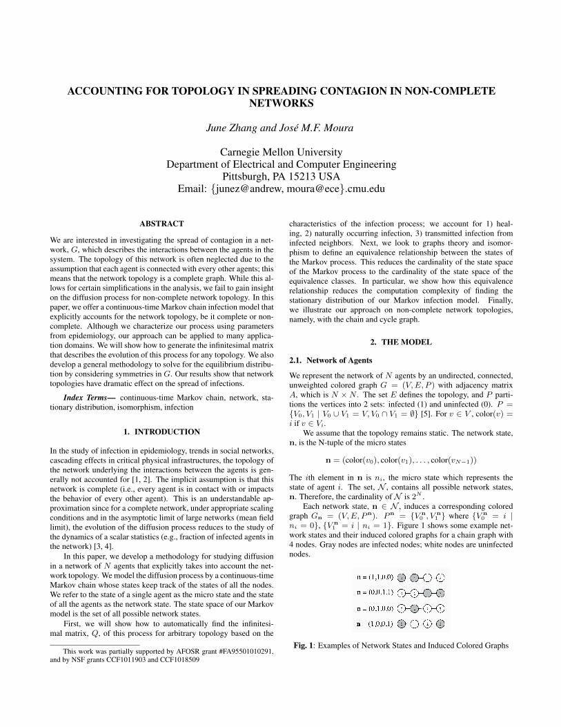
1 = i | ni = 1}. Figure 1 shows some example net-work states and their induced colored graphs for a chain graph with4 nodes. Gray nodes are infected nodes; white nodes are uninfectednodes.

Fig. 1: Examples of Network States and Induced Colored Graphs

2.2. Markov Infection Model

We will model the evolution of spreading contagion in G using con-cepts from the well-known SIS (Susceptible-Infected-Susceptible)model [3]. Let {X(t)}, (t ≥ 0) be the network state at time t. Atsome time t, X(t) = n, where n ∈ N .The process evolves basedon 3 types of events:

1. Healing. Infected nodes heal in a length of time that is expo-nentially distributed with parameter µ.

2. Exogenous infection. Uninfected nodes may naturally be-come infected in a length of time that is exponentially dis-tributed with parameter λ (assuming that there is only onetype of virus).

3. Endogenous infection. Uninfected nodes become infected bytransmission from infected neighbors in a length of time thatis exponentially distributed with parameter γ (assuming thatall infected individuals are equally contagious).

We can normalize by µ so that the process is parameterized byλµ

and γµ

.With these assumptions, we model {X(t)} as a finite state,

continuous-time Markov chain with state space N . Adapting thenotation from [6], we define 2 operators on a state of the Markovprocess, n = (n0, n1, . . . nj , . . . , nk, . . . , nN−1)

Tkn = (n0, n1, . . . , nk = 1, . . . , nN−1)

Tj•n = (n0, n1, . . . , nj = 0, . . . , nN−1)

Tk defines the operation that node k is infected. If node k is alreadyinfected, the operator does nothing. Tj• defines the operation thatnode j is healed. If node j is already uninfected, the operator doesnothing.

There are two types of state transitions in the Markov process:1) X(t) jumps to the network state where the kth node (k =

0, 1, . . . , N − 1) is infected with transition rate

q(n, Tkn) =λ

µ+

N−1∑j=0

1(nj = 1)Ajkγ

µ, n 6= Tkn (1)

where 1(·) is the indicator function, and A = [Ajk] is the adjacencymatrix ofG. The first term accounts for exogenous infections, whichdoes not dependent onG. The second term accounts for endogenousinfections, which is dependent on the topology of the network.

2) X(t) jumps to the network state where the jth node (j =0, . . . , N − 1) is healed with transition rate:

q(n, Tj•n) = 1, n 6= Tj•n (2)

2.3. Infinitesimal Matrix, Q

Using equations (1) and (2), we can generate the infinitesimal matrix,Q, which is a 2N × 2N matrix. The ith row and jth column ofQ correspond to the decimal scalar representations of the networkstates, i, j ∈ N , respectively.

The matrix Q is not symmetric, but it has symmetric struc-ture, meaning that the nonzero elements are in symmetric locations.Nonzero entries below the diagonal correspond to X(t) transition-ing to a state with one less infected individual while nonzero entriesabove the diagonal correspond to the Markov process jumping to astate with an additional infected node.

We can automatically generate Q given a network topology Gand the infection parameters λ

µand γ

µ. With Q, we can find the

equilibrium distribution, π by solving πQ = 0. For large N , thisis computationally intensive. Our next task is to utilize the conceptof isomorphism from graph theory to reduce the state space of ourMarkov process.

3. GRAPH ISOMORPHISM AND EQUIVALENCECLASSES

Recall that each network state, n, induces a colored graph Gn =(V,E, Pn). From graph theory, two graphs are considered equiva-lent if they are isomorphic to each other [5].

Two colored graphs, G = (V,E, P ) and G′ = (V ′, E′, P ′) areisomorphic, G ∼ G′, if there is a mapping φ : V → V ′ such that

1. φ is a bijection

2. (v1, v2) ∈ E if and only if (φ(v1), φ(v2)) ∈ E′ for allv1, v2 ∈ V

3. color(v) = color(φ(v)) for all v ∈ V

The first 2 conditions ensure that the uncolored graphs, (V,E)and (V ′, E′) are isomorphic. The last conditional is the additionalconstraint required by colored graph isomorphism.

3.1. Quotient Set ofN

We define the equivalence class of the network state, n, as

[n] = {x ∈ N | Gx ∼ Gn}

where ∼ is colored graph isomorphism. The set of equivalenceclasses in N is called the quotient set and is denoted as N/ ∼={[n1], [n2], . . . , [neq]}, where eq = |N/ ∼ |. The cardinalityof N/ ∼ will depend on the topology of G. However we knowthat |N/ ∼ | ≤ 2N since [ni] ∩ [nj] = ∅ for i 6= j and N =[n1] ∪ [n2] ∪ . . . ∪ [neq].

Proposition 1: If x,y ∈ [n], then π(x) = π(y). We will provethis in the Appendix.

3.2. Finding the Quotient Set,N/ ∼

With the given network, G = (V,E, P ), we can find the quotientset using the following steps:

1. Initialize: N/ ∼= ∅

2. Find the set of mappings {φ} that gives the set of uncoloredgraphs {G′} that is isomorphic to (V,E). This can be doneefficiently with existing algorithm [7]

3. While (N 6= ∅)

(a) Pick n ∈ N . It has a corresponding colored graphGn = (V,E, Pn) where Pn = {V n

0 , Vn1 }

(b) For each mapping in {φ} and each v ∈ V n1 , set

color(φ(v)) = 1 to produce colored graphs that areisomorphic to Gn. These colored graphs correspond toa set of network states, {m}

(c) Add n toN/ ∼

(d) Remove {n, {m}} fromN

3.3. Equilibrium Distribution overN/ ∼

Since all the network states in the same equivalence class have iden-tical equilibrium distribution, we can reduce the state space of theMarkov process from N to N/ ∼. The new infinitesimal matrixQeq is a eq × eq matrix. We can find the unnormalized stationarydistribution by solving πeqQeq = 0.

We normalize πeq using the relationship

|[n1]|(πeq(n1)) + . . .+ |[neq]|(πeq(neq)) = 1

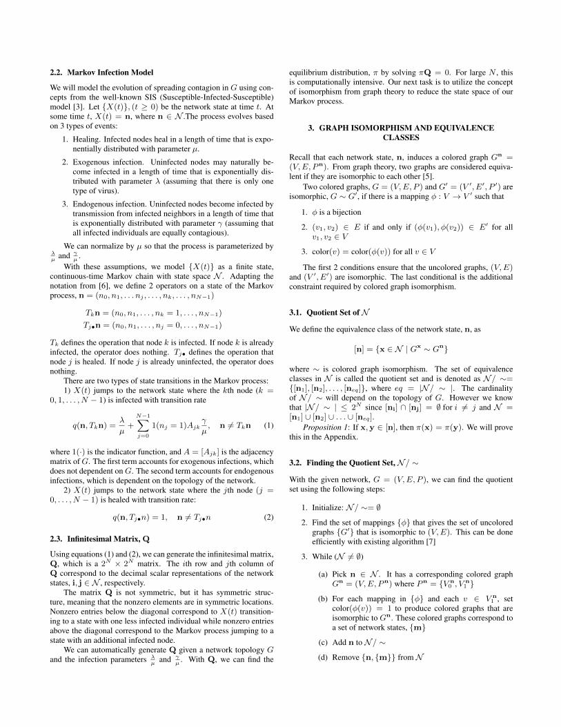
Depending on G, considering isomorphism can lead to great re-duction in the number of network states. Figure 2 shows the log-scaling of |N/ ∼ | for different network topologies. For exam-ple, in a network where N = 15, |N | = 215 = 32, 768. How-ever, if the network is a chain structure like in Figure 3a), then|N/ ∼ | = 16, 512. A cycle graph, as shown in Figure 3b), containseven more isomorphism mappings and |N/ ∼ | = 1224. Natu-rally, the graph with the most symmetry is the complete graph where|N/ ∼ | = N + 1 = 16. For the complete graph, equivalence classis determined by the number of infected nodes. This is not true fornon-complete graphs.

2 4 6 8 10 12 14 1610

0

101

102

103

104

105

N, number of nodes

Qu

otie

nt

se

t siz

e (

eq

)

Quotient Set Size vs N

2N

Chain Graph

Cycle Graph

Complete Graph

Fig. 2: log(|N/ ∼ |) vs. N = 2 to 15 for Different Graph Topolo-gies

4. RESULTS

We illustrate our model with 2 examples with parameters (N =4, λ

µ= 0.1, γ

µ= 3) for two network topologies: a chain graph,

G1, and a cycle graph, G2, as shown in Figure 3a) and Figure 3b)respectively.

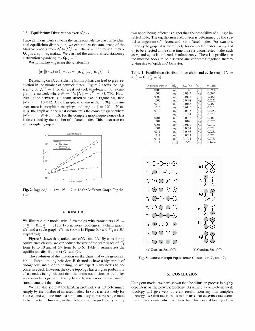
Figure 3 shows the quotient sets of G1 and G2. By consideringequivalence classes, we can reduce the size of the state space of G1

from 16 to 10 and of G2 from 16 to 6. Table 1 summarizes theequilibrium distribution of G1 and G2.

The evolution of the infection on the chain and cycle graph ex-hibit different limiting behavior. Both models have a higher rate ofendogenous infection to healing, so we expect many nodes to be-come infected. However, the cycle topology has a higher probabilityof all nodes being infected than the chain node; since more nodesare connected together in the cycle graph, it is easier for the virus tospread amongst the nodes.

We can also see that the limiting probability is not determinedsimply by the number of infected nodes. In G1, it is less likely fornode v0 and v2 to be infected simultaneously than for a single nodeto be infected. However, in the cycle graph, the probability of any

two nodes being infected is higher than the probability of a single in-fected node. The equilibrium distribution is determined by the spa-tial arrangement of infected and non infected nodes. For example,in the cycle graph it is more likely for connected nodes like v0 andv1 to be infected at the same time than for unconnected nodes suchas v0 and v3 to be infected simultaneously. There is a predilectionfor infected nodes to be clustered and connected together, therebygiving rise to ‘epidemic’ behavior.

Table 1: Equilibrium distribution for chain and cycle graph (N =4, λ

µ= 0.1, γ

µ= 3)

Network State n [n]G1πG1(n) [n]G2

πG2(n)

0000 [n1] 0.1882 [n1] 0.09681000 [n2] 0.0213 [n2] 0.00970100 [n3] 0.0163 [n2] 0.00971100 [n4] 0.0498 [n3] 0.02520010 [n3] 0.0163 [n2] 0.00971010 [n5] 0.0130 [n4] 0.01050110 [n6] 0.0375 [n3] 0.02521110 [n7] 0.1031 [n5] 0.07350001 [n2] 0.0213 [n2] 0.00971001 [n8] 0.0100 [n3] 0.02520101 [n5] 0.0130 [n4] 0.01051101 [n9] 0.0391 [n5] 0.07350011 [n4] 0.0498 [n3] 0.02521011 [n9] 0.0391 [n5] 0.07350111 [n7] 0.1031 [n5] 0.07351111 [n10] 0.2790 [n6] 0.4484

(a) Quotient Set of G1 (b) Quotient Set of G2

Fig. 3: Colored Graph Equivalence Classes for G1 and G2

5. CONCLUSION

Using our model, we have shown that the diffusion process is highlydependent on the network topology. Assuming a complete networktopology will give very different results from any non-completetopology. We find the infinitesimal matrix that describes the evolu-tion of the disease, which accounts for infection and healing of the

nodes in any topology. We use the concept of graph isomorphismto reduce the state space of the Markov process to expedite thecalculation for the stationary distribution.

6. REFERENCES

[1] I. Dobson, B.A. Carreras, and D.E. Newman, “A branchingprocess approximation to cascading load-dependent system fail-ure,” Hawaii International Conferences on System Sciences,Jan. 2004.

[2] N. Boccara, Modeling complex systems, Springer Verlag, 2010.

[3] M. O. Jackson, Social and Economic Networks, Princeton Uni-versity Press, 2008.

[4] A. Santos and J.M.F. Moura, “Emergent behavior in large scalenetworks,” Conference on Decision and Control, Dec. 2011.

[5] A. Lal and D. van Melkebeek, “Graph isomorphism for col-ored graphs with color multiplicity bounded by 3,” Tech. Rep.,Citeseer, 2005.

[6] F.P. Kelly, Reversibility and stochastic networks, vol. 40, WileyNew York, 1979.

[7] Gabor Csardi and Tamas Nepusz, “The igraph software pack-age for complex network research,” InterJournal, vol. ComplexSystems, pp. 1695, 2006.

[8] G. Royle C. Godsil, Algebraic Graph Theory, Springer-Verlag,2001.

[9] S. Karlin H. M. Taylor, An Introduction to Stochastic Modeling,Academic Press, 3rd edition, 1998.

A. PROOF OF PROPOSITION 1

If x,x ∈ [n], then π(x) = π(x).x and x are in the same same equivalence class so there is a

mapping, φ, such that the induced graph Gx = (V,E, Px) is colorisomorphic to Gx = (φ(V ), E, Px). Gx and Gx have the sameadjacency matrix, A. Using Lemma 1.31 from [8], which statesthat node vi ∈ Gx, (i = 0, 1, . . . N − 1) and node φ(vi) ∈ Gx

have the same number of neighbors. This means that∑N−1k=0 Aki =∑N−1

k=0 Akφ(i).The equilibrium distribution, π, satisfies the global balance

equation:

π(x)

(N−1∑k=0

q(x, Tkx) +

N−1∑j=0

q(x, Tj•x)

)= (3)

N−1∑k=0

π(Tkx)q(Tkx,x) +

N−1∑j=0

π(Tj•x)q(Tj•x,x)

π(x)

N−1∑φ(k)=0

q(x, Tφ(k)x) +

N−1∑φ(j)=0

q(x, Tφ(j)•x)

= (4)

N−1∑φ(k)=0

π(Tφ(k)x)q(Tφ(k)x,x)

+

N−1∑φ(j)=0

π(Tφ(j)•x)q(Tφ(j)•x,x)

Note that Tkx and Tφ(k)x are in the same equivalence class.The Tk operator represents a coloring of the kth node in Gx whileTφ(k) represents a coloring of the φ(k)th node in Gx. This coloring,together with the mapping φ, satisfy the 3 conditions of color iso-morphism. Similarly, Tj•x and Tφ(j)•x are in the same equivalenceclass.

Consider the transition rates:

q(x, Tj•x) = 1 = q(x, Tφ(j)•x)

q(x, Tkx) =λ

µ+

N−1∑j=0

1(nj = 1)Ajkγ

µ

=λ

µ+

N−1∑j=0

1(nj = 1)Ajφ(k)γ

µ

= q(x, Tφ(k)x)

By the same reasoning,

q(Tkx,x) = q(Tφ(k)x,x)

q(Tj•x,x) = q(Tφ(j)•x,x)

Equations (3) and (4) represents two linear systems with iden-tical coefficients. Since finite state Markov process always has anunique equilibrium distribution, the solution to the linear systemsmust be unique as well. Therefore, π(x) = π(x) when x,x ∈ [n].

A.1. Finite State Continuous-Time Markov Process Review

We model the diffusion process by a finite state continuous-timeMarkov chain, {X(t)}(t ≥ 0) with states {0, 1, . . .M}. We willonly consider an aperiodic, irreducible, time homogenous, finitestate Markov process [9]. The process is characterized by

q(i, j) = limτ→0

Pij(τ)

τ, j 6= i

= 0, j = i

where Pij(t) is the transition probability of going from state i tostate j in t duration. It is also the is the {i, j} entry in the matrixP(t). Have

q(i) =

M∑j=0,j 6=i

q(i, j)

The rates, q(i) and q(i, j), provide us with the infinitesimal descrip-tion of the Markov process. The amount of time that the process willremain in state i is exponentially distributed with parameter q(i). Wecan express the transition rates as the infinitesimal matrix, Q, where

Q =

−q(0) q(0, 1) . . . q(0,M)q(1, 0) −q(1) . . . q(1,M)

...q(M, 0) q(M, 1) . . . −q(M)

The differential equation that governs the evolution of P(t) is

P′(t) = P(t)Q

We can find π by solving the system of equations

0 = πQ =[π(0) π(1) . . . π(M)

]Q

with the additional constraint that∑Mi=0 π(i) = 1.