Accounting for Uncertainty and Complexity in the

Realization of Engineered Systems

Warren F. Smith1, Jelena Milisavljevic

2, Maryam Sabeghi

2, Janet K. Allen

2,

and Farrokh Mistree2

1 School of Engineering and IT, University of NSW Canberra, ACT, Australia 2 Systems Realization Laboratory, University of Oklahoma, Norman, OK, USA

Abstract. Industry is faced with complexity and uncertainty and we in academ-

ia are motivated to respond to these challenges. Hence this paper is the product

of thoughts for exploring the model-based realization of engineered systems.

From the perspective that the activity of designing is a decision making process,

it follows that better decisions will be made when a decision maker is better in-

formed about the available choices and the ramification of these choices. Pre-

sented in this paper, in the context of an example of designing a small thermal

plant, is a description of an approach to exploring the solution space in the pro-

cess of designing complex systems and uncovering emergent properties. The

question addressed is that given a relevant model, what new knowledge, under-

standing of emergent properties and insights can be gained by exercising the

model?

Keywords: Decision-based, Model-based, Compromise, Complex Systems, So-

lution Space Exploration, Decision Support Problem

1. MOTIVATION

Designing, in an engineering context, is an activity that seeks to deliver a descrip-

tion of a product to satisfy a need in response to a stated objective and/or set of re-

quirements. In the process, it may involve invention and/or the application of science

and engineering knowledge to resolve a solution. Given that multiple solutions may

be proposed with differing measures of merit, it follows that the paramount role of a

designer is that of a decision maker. It is further argued that understanding the inher-

ent choices and risks within the context of a design lead to justifiable decisions. In an

age where issues such as efficiency, equity, sustainability and profitability are equally

valid decision drivers the motivation to develop theories and approaches to explore

the design and aspiration spaces is strong. Indeed, this is what motivates the academic

design community in general and the authors of this paper in particular.

2. FRAME OF REFERENCE

Design choices can be explored through first building sufficiently detailed and valid

mathematical models, and then exercising these models and seeking understanding of

their behavior and the emergent properties (those that are unforeseen and influenced

by uncertainty). Such models can very quickly become very complicated. Organized

complexity in the context of systems theory is said to arise from the combination of

parts that form a system but the behavior of the system is not necessarily controllable

or predictable from knowledge of the parts alone. Disorganized complexity in contrast

is a reflection of the random and statistical variability of the parts and the subsystems

and system they form. It follows that to grow complex system knowledge requires the

management of aspects of both complication (complexity) and uncertainty. Managing

uncertainty raises concerns such as those due to the imprecise control of process pa-

rameters, the incomplete knowledge of phenomena, the incomplete models and in-

formation aggregation, and the need to explore alternatives. Managing issues of com-

plication include dealing with the trade-off between accuracy and computational time,

the levels of interdependencies between parts, and the allocation of resources to ex-

ploring the solution and aspiration spaces. It follows that the challenge for engineers

is the creation of knowledge about the system and the challenge encompasses captur-

ing tacit knowledge, building the ability to learn from data and cases, and developing

methods for guided assistance in decision making.

The authors have adopted a model based approach in pursuing these challenges

recognizing that models can have different levels of fidelity, they can be incomplete

and possibly inaccurate (particularly during the early stages of design).

2.1 The Decision Support Problem

Used is the Decision Support Problem (DSP) construct that is based on the philosophy

that design is fundamentally a decision making and model-based process [1, 2]

. A tai-

lored computational environment known as DSIDES has been created as an imple-

mentation of the method. The DSP and DSIDES are well documented in [3-7]

.

Reported applications of this approach include the design of ships, damage tolerant

structural and mechanical systems, design of aircraft, mechanisms, thermal energy

systems, composite materials and the concurrent design of multi-scale, multi-

functional materials and products. A detailed set of early references to these applica-

tions is presented in [8]

. Key applications more recently span specification develop-

ment [9, 10]

, robust design [11-14]

, product families [15-17]

, the integrated realization of

materials and products [18-22]

, and a variety of mechanical systems [23-26]

.

The nature of a decision and model-based approach to designing through model-

ling the physical world is portrayed in Figure 1. Once a model is appropriately formu-

lated, DSIDES, with its operations research tools (traditionally an adaptive sequential

linear programming algorithm delivering vertex solutions), is used to deduce “model

conclusions” [5]

. Where dilemmas exist this process may be iterative in nature and

demand significant justification. It thus becomes imperative to be able to describe and

understand the design and aspiration spaces and to be able to explore these spaces.

Key is the concept of two types of decisions (namely, selection and compromise)

and that any complex design can be represented through mathematically modelling a

network of compromise and selection decisions [4, 6]

. Being able to work with the

complexity of these decision networks is also a foundational construct as are the axi-

oms of the approach as detailed in References [4, 6]

.

In reflecting on the compromise DSP, parallels with the “demands” and “wishes”

of Pahl and Bietz [27]

can be drawn. The demands are met by satisfaction of the DSP

constraints and bounds and the wishes are represented by the goals. Collectively, the

constraints and bounds define the feasible design space and the goals define the aspi-

ration space. The feasible and aspiration spaces together then form the solution space.

Note that a selection DSP can be formulated as a compromise DSP [28]

where the key

words “Given”, “Find”, “Satisfy” and “Minimize” are used.

Fig. 1. Modelling the Physical World

2.2 Understanding the Solution Space

A strategy for identifying a possible solution space and exploring it using tools within

DSIDES includes:

Firstly, discover regions where feasible designs exist based on satisfying the con-

straints and bounds or where they might exist by minimizing constraint violation.

Secondly, from the neighborhood of feasible or near feasible regions frame the

feasible design space extremities using a preemptive (lexicographic minimum) rep-

resentation of the goals in a higher order search.

Thirdly, having framed the space and the zones of greatest interest, move between

the extremes generating deeper understanding and exploring tradeoffs using an Ar-

chimedean (weighted sum) formulation of the goals.

Our focus in this paper is on the first two steps. To discover feasible regions, zero,

first and second order methods are currently available in DSIDES.

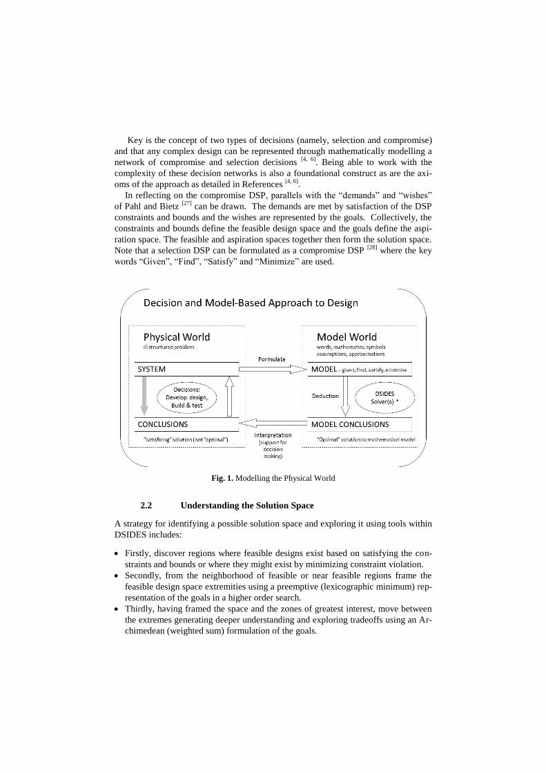
This overall process is conceptually reflected in Figure 2 where over time

knowledge, confidence and utility increase while converging to a recommended deci-

sion. The decisions are made through a series of diverging, synthesizing and conver-

gent decision making processes. As will become clearer, various tools may be used to

support different decisions.

Fig. 2. Modelling and Decision Timeline

The most rudimentary approach within DSIDES is a zero order search referred to

as XPLORE. Based on the algorithm of reference [29]

, it is used to test a range of de-

signs within the stated system variable bounds. The best N designs are kept providing

candidate starting points for higher order searches. A second method utilizing a pat-

tern search algorithm is also available within the INITFS (Initial Feasible Solution)

module. Used in series, these methods can assist greatly in delivering the Adaptive

Linear Programming (ALP) algorithm a starting point from which the likelihood of

achieving greater understanding of the solution space is high. In the case of a multi-

modal solution space a variety of starting points are employed.

Various methods may be applied to conduct post solution analysis on the data gen-

erated including visualization through the use of various plots. Given that in ALP is a

linear based simplex solver, the opportunity to explore sensitivity using primal and

dual information exists. Also provided in DSIDES is information about the monotonic

characteristics of the model. In concert, all these elements contribute to the effective

modelling, framing, exploration and dilemma resolution that is necessary when con-

sidering the design of complex systems.

3. SCENARIO FOR THE EXAMPLE

The study at the core of this paper is being developed to support the growing research

effort within the Systems Realization Laboratory at the University of Oklahoma. Cur-

rent research interests in the laboratory inter alia span complex systems, dilemma

management, design space modelling and exploration, post solution analysis, and

sustainability when considering economic, socio-cultural, and environmental issues.

One domain allowing all these matters to be explored is thermal systems.

There are many possible applications for small scale “power” plant systems that

make direct mechanical use of the power produced or that run small generators to

produce electricity. Examples include provision of power to equipment in farming

irrigation systems, driving reverse osmosis systems to produce fresh water for remote

communities and generating electricity for general use in small collectives in both 1st

and 3rd

world environments.

A common approach given an available heat source is to build such a system

around the Rankine cycle, a mathematical representation of a “steam” operated heat

engine. A schematic representation of the Rankine cycle is shown in Figure 4 where

the primary components of the system are a power producing turbine, a pump to pres-

surize the flow to the turbine and two heat exchangers; a condenser and a heater. In

the context of building a model using a decision-based approach to design, such a

thermal system affords complexity to be developed and dilemmas to be managed and

resolved, both hypothetically and practically. Modelling the Rankine cycle represents

Stage 1 of the model development and will be referred to herein as the foundational

example model. Future expansion within the laboratory will deal with heat source

issues (to the left in Figure 3) and power use issues (to the right in Figure 3) and the

choice of working fluids. The common working fluid in a Rankine cycle is water.

Uses of other fluids (often organic in chemistry) have given rise to the development

of “organic Rankine cycles”. Of course geometric specification and design analysis of

physical elements in the system also represent opportunities for model and design

space exploration.

Fig. 3. Stage 1 Model Schematic Fig. 4. Rankine Cycle

(Temperature v Entropy)

4. THE FOUNDATIONAL EXAMPLE MODEL

The foundational example model is defined by the cycle’s maximum and minimum

pressures and maximum temperature (PMAX, PMIN and TMAX). Energy is trans-

ferred to the closed loop Rankine cycle through a heat exchanger. The heat exchanger

is assumed to be of a counter flow design where the key characteristic is the maxi-

mum temperature of the heating flow (TMAXE).

From a decision based design approach, the determination of satisficing1 values of

these variables represents a coupled compromise-compromise DSP dealing with the

Rankine cycle (PMAX, PMIN and TMAX) and the heat exchanger (TMAXE) respec-

tively. Two additional decisions have been built into the template of the current mod-

el, namely, the selection of the fluids for both the heating and Rankine cycle loops.

Therefore, in concept the current model is a compromise-compromise-selection-

selection problem. Further complexity in the model will be developed in due course to

reflect aspects of the mechanical design of the system components ( eg., dimensions).

The ideal Rankine cycle involves 4 processes, as shown graphically in the Tem-

perature (T) versus Entropy (S) plot in Figure 4. There are two adiabatic isentropic

processes (constant entropy) and two isobaric processes (constant pressure).

Referring to Figure 4,

①-② adiabatic pumping of the saturated liquid from PMIN to PMAX

②-④ isobaric heat addition in heat exchanger to TMAX,

④-⑤ adiabatic expansion in the turbine from PMAX to PMIN producing

power with the possibility of wet steam exiting the turbine, and

⑤-① isobaric heat loss in the condenser.

The isothermal segments represent moving from saturated liquid to saturated va-

por in the case of ③ in the heater and the reverse in the condenser between ⑤-①.

The key thermodynamic properties of the working fluid(s) are determined using

REFPROP [30]

. For the purposes of this paper focus has been placed on the compro-

mise-compromise aspects and a number of system variables have been treated as pa-

rameters. One such simplification is the use of water as the working fluid in both

loops.

The combined model may be summarized using the compromise key words as:

GIVEN

Water as the fluid in the Rankine cycle

Water as the heat transfer medium in the heat exchanger

The minimum pressure in the Rankine cycle (PMIN – defined as a parameter)

Ideal Rankine cycle thermodynamics

Ideal heat transfer in the heat exchanger

Thermodynamic fluid properties (determined using REFPROP)

1 Satisficing is a decision-making strategy or cognitive heuristic that entails searching

through the available alternatives until an acceptability threshold is met. This is contrasted

with optimal decision making, an approach that specifically attempts to find the best alterna-

tive available. Wikipedia.

FIND

x, the system variables

PMAX Maximum pressure in the Rankine cycle

TMAX Maximum temperature in the Rankine cycle

TMAXE Maximum temperature of the heating fluid

d- and d

+, the deviation variables

SATISFY

The system constraints:

Temperature delta for maximums in exchanger

Moisture in turbine less than upper limit

Rankine cycle mas flow rate less than upper limit

Temperature at ④ ≥ temperature at ③

Quality at ④ is superheated vapor

TMAXE greater than TMINE by at least TDELE

TMINE ≥ temperature at ② by at least TDELC

Ideal Carnot cycle efficiency greater than system efficiencies (sanity check)

Temperatures within valid ranges for REFPROP fluid database

The system variable bounds (xjmin

≤ xj ≤ xjmax

):

500 ≤ PMAX ≤ 5000 (kPa)

350 ≤ TMAX ≤ 850 (K)

350 ≤ TMAXE ≤ 850 (K)

The system goals:

Achieve zero moisture in steam leaving the turbine (ie., steam quality of 1)

Maximize Rankine cycle efficiency where RCEFF = (Pturbine – Ppump)/Qin

Maximize temperature exchanger efficiency

where TEFFEX = (TMAXE-TMINE)/(TMAXE-TEMP2)

Maximize system efficiency indicator 1 where SYSEF1 = (Pturbine – Ppump)/Qout

Maximize system efficiency indicator 2 where SYSEF2 = RCEFF*TEFFEX

Maximize heat transfer effectiveness in exchanger

where HTEFF = f(heat transfer coefficient, geometry, flow rates etc.)

MINIMIZE

The deviation function, Z(d-, d

+) = [f1(d

-, d

+), …,fk(d

-, d

+)]

where the deviation function is expressed in a preemptive form.

The six system goals in the example have been placed at six levels of priority in the

implemented preemptive model. The implication is that the first level goal function

will be satisfied as far as possible and then while holding it within a tolerance; the

second level goal function will be addressed. When the second has been so condition-

ally minimized it will be held within its tolerance and then the third goal will be

worked upon; and so on in an attempt to address all the goals across all levels.

Achieving satisfaction of the higher priority goals may cause the sacrifice of

achievement of the lower priority goals. By prioritizing the goals differently, compar-

ison may show competing goals driving the solution process in different directions.

By grouping more than one goal at the same level, an Archimedean (weighted sum)

approach can be accommodated.

5. VALIDATION OF THE MODEL

Structural validity as it applies to a computer code infers that the logic and data flows

between modules are correct. This does not guarantee accuracy. Performance validity

is associated with the accuracy of the results achieved as measured against reliable

benchmarks and/or reasoned argument (other published work, known physical charac-

teristics etc.).

5.1 Structural Validity of the Model

The compromise DSP is a hybrid multi-objective construct and this approach to

designing has been validated through use [6]

. The primary solver in DSIDES is an

Adaptive Linear Programming algorithm, and it has also been described and validated

elsewhere [5]

. The current instantiation has also been shown to replicate some standard

test problems. The REFPROP database is a key thermodynamic property model from

NIST [30]

and the NIST supplied subroutines and fluid files have been used. The total

system has been integrated in a FORTRAN environment using G FORTRAN compil-

ers on a PC platform. The functioning of the code has been successfully demonstrated

to reproduce results consistent with text books and other programs providing thermo-

dynamic properties of fluids.

Consistency and logical relationship between the constructs were checked by test-

ing several inputs and reviewing the expected outputs, e.g., thermodynamic properties

of water at different pressures and temperatures.

5.2 Performance Validity of the Model

Performance validity was checked through exercising the thermal model, i.e., investi-

gation of the model by parametric study such as net power output. For instance, since

the power is a function of Rankine flow rate, it is expected that higher flow rates are

necessary to produce higher power. This was verified and is discussed in Section 6.

The next step for performance validity of the model was through checking the be-

havior of the goals. This model includes six goals, five of which estimate measures of

efficiency: the Rankine cycle efficiency, the heat exchanger efficiency, two formula-

tions of system efficiency and the heat exchanger effectiveness. By exploring differ-

ent possibilities in the goal priorities for the example and by examination of the mon-

otonicity of the goals [31]

it was discovered that the prioritization of the efficiency

goals in a preemptive formulation will drive the system in two directions.

If prioritization is given to the Rankine cycle efficiency and/or system efficiency

formulation 1 the solutions are of high temperature and high pressure character. In

discussing the results this ordering of priority will be referred to as “Order 1”. In con-

trast, low temperature and low pressure solutions are preferred if the heat exchanger

efficiency, system efficiency formulation 2 and/or heat transfer effectiveness are pri-

oritized (Order 2). This behavior of the model is appropriate and predictable given the

model goal formulations.

6. DISCUSSION OF RESULTS

Consider that a plant producing a baseline of 25kW is required and that higher powers

are sought but the maximum steam that can be produced is 0.1 kgs-1

. What are the

characteristic values that define the Rankine cycle and the heat exchanger?

In answering this question, a two-step process using DSIDES is used, firstly with

the XPLORE grid search module and then with the ALP algorithm.

As described in Section 4, variable bounds have been defined but do they encom-

pass feasible designs? Using XPLORE, this question is examined. Presented in Figure

5 is a plot of TMAX versus PMAX showing discrete tested combinations that lead to

feasible designs for 25, 50 and 70kW cases. Feasible designs exist where the con-

straint violation is zero. The extent of the plot reflects the bounds of each system vari-

able. The contraction in the number of designs and the size of the design space at least

in the two dimensions shown as power increases is clearly evident. The area covered

by these can be interpreted as being representative of the feasible design space(s).

Further use of EXPLORE can and has in this example been made to examine the

regions where goals are fully satisfied or at least minimized. Being keen to ensure

longevity of the plant, the operational requirement is that moisture in the steam exit-

ing the turbine is minimized. Therefore, the Level 1 priority goal for all results pre-

sented is that of minimizing moisture. If this were the only goal specified it can be

shown as in Figure 6 that there are many designs that could achieve less than 5%

moisture while producing 25 kW or 50 kW. Shown in Figure 7 are those designs with

zero percent moisture.

Fig. 5. Feasible designs using XPLORE (less than 12% moisture)

It follows that other goals need to be subsequently specified to achieve singular

(local) convergence. For the 25 kW designs, using the XPLORE data, if some mois-

ture is allowed (up to 12%) higher Rankine cycle efficiencies can be achieved with

designs depicted in the region shown in top right of Figure 8 (efficiencies better than

27.5%). However, constraining the designs to have zero moisture caps the best Ran-

kine cycle efficiency found at 25% (PMAX 2136 kPA and TMAX 759 K), signifi-

350

450

550

650

750

850

500 2500 4500

TMA

X (

K)

PMAX (kPa)

25kW

50kW

75kW

cantly to the left of the Figure 8 cluster. This reflects the best “Order 1” XPLORE

solution.

Fig. 6. Feasible designs with moisture less

than 5% using XPLORE

Fig. 7. Feasible designs with 0.000% mois-

ture using XPLORE

Considering the second system efficiency goal representation, SYSEF2, if set as

priority one, values of 16% in the lower left region shown in Figure 8 are possible. If,

constraining the designs to have zero moisture caps the best SYSEF2 value found is

12% (PMAX 909 kPA and TMAX 668 K), significantly higher than the Figure 8

cluster. This reflects the best “Order 2” XPLORE solution.

To summarize, higher Rankine cycle efficiencies are achieved with high tempera-

tures and high pressures. In contrast, the higher system efficiencies result from low

temperatures and low pressures. And, to achieve zero moisture in the turbine, the

requirement is for high temperatures with lower pressures. Clearly, the right decision

is not straightforward.

Fig. 8. Trade-offs for feasible designs for 25kW using XPLORE (less than 12% moisture)

350

450

550

650

750

850

500 2500 4500

TMA

X (

K)

PMAX (kPa)

25kW

50kW350

450

550

650

750

850

500 2500 4500

TMA

X (

K)

PMAX (kPa)

25kW

50kW

350

450

550

650

750

850

500 1500 2500 3500 4500

TMA

X (

K)

PMAX (kPa)

Higher System Efficiency 2

Higher Rankine Cycle Efficiency

Zero Moisture

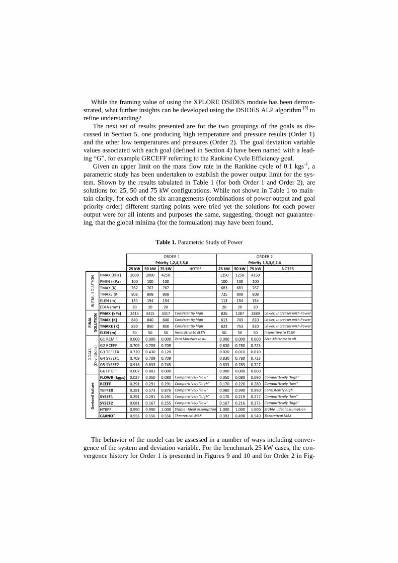
While the framing value of using the XPLORE DSIDES module has been demon-

strated, what further insights can be developed using the DSIDES ALP algorithm [5]

to

refine understanding?

The next set of results presented are for the two groupings of the goals as dis-

cussed in Section 5, one producing high temperature and pressure results (Order 1)

and the other low temperatures and pressures (Order 2). The goal deviation variable

values associated with each goal (defined in Section 4) have been named with a lead-

ing “G”, for example GRCEFF referring to the Rankine Cycle Efficiency goal.

Given an upper limit on the mass flow rate in the Rankine cycle of 0.1 kgs-1

, a

parametric study has been undertaken to establish the power output limit for the sys-

tem. Shown by the results tabulated in Table 1 (for both Order 1 and Order 2), are

solutions for 25, 50 and 75 kW configurations. While not shown in Table 1 to main-

tain clarity, for each of the six arrangements (combinations of power output and goal

priority order) different starting points were tried yet the solutions for each power

output were for all intents and purposes the same, suggesting, though not guarantee-

ing, that the global minima (for the formulation) may have been found.

Table 1. Parametric Study of Power

The behavior of the model can be assessed in a number of ways including conver-

gence of the system and deviation variable. For the benchmark 25 kW cases, the con-

vergence history for Order 1 is presented in Figures 9 and 10 and for Order 2 in Fig-

25 kW 50 kW 75 kW 25 kW 50 kW 75 kW

PMAX (kPa) 2000 2000 4250 1250 1250 4250

PMIN (kPa) 100 100 100 100 100 100

TMAX (K) 767 767 767 683 683 767

TMAXE (K) 808 808 808 725 808 808

ELEN (m) 154 154 154 113 154 154

EDIA (mm) 20 20 20 20 20 20

PMAX (kPa) 3415 3415 3417 826 1287 2889

TMAX (K) 840 840 840 613 743 810

TMAXE (K) 850 850 850 623 753 820

ELEN (m) 50 50 50 50 50 50

G1 RCMIT 0.000 0.000 0.000 0.000 0.000 0.000

G2 RCEFF 0.709 0.709 0.709 0.830 0.780 0.723

G3 TEFFEX 0.720 0.430 0.120 0.020 0.010 0.010

G4 SYSEF1 0.709 0.709 0.709 0.830 0.780 0.723

G5 SYSEF2 0.918 0.833 0.745 0.833 0.783 0.727

G6 HTEFF 0.007 0.001 0.000 0.000 0.000 0.000

FLOWR (kgps) 0.027 0.050 0.080 0.050 0.080 0.090

RCEFF 0.291 0.291 0.291 0.170 0.220 0.280

TEFFEX 0.281 0.573 0.876 0.980 0.990 0.990

SYSEF1 0.291 0.291 0.291 0.170 0.219 0.277

SYSEF2 0.081 0.167 0.255 0.167 0.216 0.273

HTEFF 0.990 0.990 1.000 1.000 1.000 1.000

CARNOT 0.556 0.556 0.556 0.392 0.498 0.540

NOTES

ORDER 1

Priority 1,2,4,3,5,6

Consistently high

Insensitive to ELEN

INIT

IAL

SO

LUT

ION

NOTES

ORDER 2

Priority 1,5,3,6,2,4

De

riv

ed

Va

lue

s

Comparitively "low"

Comparitively "high"

Comparitively "low"

Comparitively "high"

Comparitively "low"

Stable - Ideal assumption

Theoretical MAX

GO

ALS

(De

via

tio

ns)

Zero Moisture in all

FIN

AL

SO

LUT

ION Consistently high

Consistently high

Lower, increases with Power

Insensitive to ELEN

Zero Moisture in all

Lower, increases with Power

Lower, increases with Power

Consistently high

Comparitively "low"

Comparitively "high"

Stable - Ideal assumption

Theoretical MAX

Comparitively "high"

Comparitively "low"

ures 11 and 12. All curves reach a stable final steady state. In the case of Order 1, zero

moisture in the turbine was not achieved until iteration 9. This aspect dominated the

solution process to this point. However, GRCEFF and GSYSE1 which are superim-

posed are seen to be generally decreasing. The reverse is true for Order 2. For Order

2, zero moisture was achieved from iteration 5 from which point reductions in

GSYSE2, GEXEFF and GHTEFF are evident. Clearly an indicator of excess capacity

in considering the baseline 25 kW case is that the flow rate in the turbine is well be-

low the defined bound on this variable of 0.1. In framing and exploring a design mod-

el, the nature of the specified variable bounds needs to be understood. Some are set

based on true physical constraints and some are arbitrary.

The parametric study of power has provided the flow rate results depicted in Figure

13. For Order 1 where Rankine cycle efficiency is favored, the flow rate is lower be-

cause of the improved efficiency. Extrapolating to where both flow rate curves would

intersect the 0.1 kgs-1

upper bound, it would appear that approximately 90 kW would

be available in the modelled ideal system. A companion plot of the Rankine cycle

efficiency versus power is given in Figure 14 where a consistently high efficiency is

achieved for Order 1. The efficiencies produced under Order 2 are forced to increase

in order to produce the higher power demands. In contrast, the final plot presented,

Figure 15, is used to highlight that by prioritizing the goals as per Order 2, higher

values of system efficiency as measured by the second formulation can be achieved.

This formulation is a product of the efficiencies of the two primary system compo-

nents, exchanger and Rankine cycle. Because of the idealized efficiency of the ex-

changer being higher than that of the Rankine cycle, this term dominates and there-

fore drives the solution to the lower temperatures and pressures that suit the exchang-

er. The monotonically increasing curves of Figure 15 further suggest that higher over-

all efficiencies will come with higher power.

Fig. 9. Order 1 system variable (25kW)

convergence plotted against iteration,

Fig. 10. Order 1 deviation variable (25kW)

convergence plotted against iteration,

(lower values preferred,

GRCEFF and GSYSE1 superimposed)

0

500

1000

1500

2000

2500

3000

3500

4000

1 2 3 4 5 6 7 8 9 1011

PM

AX

(kP

a), T

MA

X &

TM

AX

E (K

) PMAX

TMAX

TMAXE

0

0.2

0.4

0.6

0.8

1

1 2 3 4 5 6 7 8 9 10 11

GRCEFF

GSYSE1

GEXEFF

GSYSE2

GHTEFF

Fig. 11. Order 2 system variable (25kW)

convergence plotted against iteration,

Fig. 12. Order 2 deviation variable (25kW)

convergence plotted against iteration,

(lower values preferred, GRCEFF and

GSYSE1 superimposed)

Fig. 13. Rankine Cycle Mass Flow Rate, FLOWR versus Power Output

(Order 1 – solid line; Order 2 – dashed line)

Fig. 14. Rankine Cycle Efficiency versus

Power Output

(Order 1 – solid line; Order 2 – dashed line)

Fig. 15. System Efficiency 2, GSYSE2,

versus Power Output

(Order 1 – solid line; Order 2 – dashed line)

500

600

700

800

900

1000

1100

1200

1300

1 3 5 7 9 11 13 15

PM

AX

(kP

a), T

MA

X &

TM

AX

E (K

)

PMAX

TMAX

TMAXE

0

0.2

0.4

0.6

0.8

1

1 2 3 4 5 6 7 8 9 101112131415

GSYSE2

GEXEFF

GHTEFF

GRCEFF

GSYSE1

R² = 0.9942

R² = 0.9231

0.000

0.020

0.040

0.060

0.080

0.100

0 50 100

FLO

WR

, kg/

s

Power Output, kW

R² = 0.9973

0.000

0.100

0.200

0.300

0.400

0 50 100

Ran

kin

e C

ycle

Eff

icie

ncy

Power Output, kW

R² = 1

R² = 0.9981

0.000

0.100

0.200

0.300

0.400

0 50 100

Syst

em

Eff

icie

ncy

2

Power Output, kW

7. CONCLUDING REMARKS

Industry is faced with complexity and uncertainty and we in academia are motivated

to respond to these challenges. Hence this paper is the product of thoughts for explor-

ing the model-based realization of engineered systems. What new knowledge, under-

standing of emergent properties and insights can be gained by exercising the model?

In summary, perhaps the conflict expressed in Figure 8 best reflects the discovery of

emergent properties from the system. Pursuing the questions further leads to a growth

in understanding exemplified by the findings based on the information presented in

Figures 13, 14 and 15.

While the results presented in Section 6 are for a relatively simple case and some

variation has been dealt with parametrically, the model is structured to deal with sig-

nificantly increased complexity through the integration of more detailed analysis.

Possibilities include adding features to incorporate real as opposed to ideal character-

istics of the Rankine cycle (e.g., pipe losses, pumping losses). The mechanical design

and more detailed sizing of components could also be added as could higher order

heat transfer models that address the time and material dependencies of conduction in

the heat exchangers. Including design robustness considerations are also desirable.

In Section 1, it was indicated that the thermodynamically oriented example pre-

sented herein is anticipated to provide the foundation for a significant body of future

work and doctoral study in the “Systems Realization Laboratory” at the University of

Oklahoma. Therefore, to conclude, the possible directions to be taken are identified.

Managing (Organized) Complexity – Future Work

In this work, the main focus will be on model development to grow complexity and

the physical realism of the system (e.g., dimensions and materials). This will facilitate

more detailed and practically-useful design input for small scale “power” plant sys-

tems through simulation.

Given the existing Stage 1 model, Stage 2 will include expansion focused on heat

source issues: representation of aspects of the heat exchanger (boiler). While the cur-

rent goals are moisture and efficiency based, the intent is to also model economic

considerations. The selection decisions for the working fluids will be developed in

line with options for lower temperatures and pressures applications inherent in an

organic Rankine cycle.

For the heat exchanger, the first steps taken will include the thermodynamic mod-

elling to address conduction leading to the specification of the required geometry

(e.g., length and diameter of inner and outer pipe and material choice). Possibilities

beyond Stage 2 include similar work with other system components as alluded to in

Section 3 (“left” and “right” sides and further Rankine cycle refinements).

Managing (Disorganized Complexity) Uncertainty – Future Work

In this work, the focus will be on developing the modelling with respect to managing

uncertainty. The research plan includes using the expanded thermal model, adding

robustness considerations to address uncertainty and exploring the solution space

using an Archimedean formulation, with sensitivity and post solution analysis.

In this paper the feasible solution space of the example thermal system was ex-

plored using a preemptive representation. As the example system model complexity

grows, greater conflict in the goals is also anticipated. The next step, as described as

the third in Section 2.2, is to explore the solution space by moving between the ex-

tremes to generate deeper understanding of the tradeoffs. An Archimedean (weighted

sum) formulation of the goals can be utilized for this purpose.

Sensitivity and post solution analysis can be performed on a system by changing

the bounds, relaxing or adding constraints, finding the limit (bounds) of the parame-

ters and changing the target input data to be documented for the designer. Use of pri-

mal and dual information from a linear model (as generated by the ALP algorithm)

may also provide new insights in exploring such a complex system.

Acknowledgments. We thank the University of New South Wales, Australia, for the

financial support provided to Warren Smith for him to spend a sabbatical year at the

Systems Realization Laboratory at the University of Oklahoma, Norman. Jelana Mili-

savljevic acknowledges the financial support from NSF Eager 105268400. Maryam

Sabeghi acknowledges the NSF Graduate Research Fellowship that funds her gradu-

ate studies. Janet K. Allen and Farrokh Mistree acknowledge the financial support

that they received from the John and Mary Moore chair account and the LA Comp

chair account, respectively.

References

1. Marston, M., Allen, J.K., and Mistree, F., The Decision Support Problem

Technique: Integrating Descriptive and Normative Approaches. Engineering

Valuation & Cost Analysis, Special Issue on Decision-Based Design: Status

and Promise, 2000. 3: p. 107-129.

2. Muster, D. and Mistree, F., The Decision Support Problem Technique in

Engineering Design. The International Journal of Applied Engineering

Education, 1988. 4(1): p. 23-33.

3. Mistree, F., Smith, W.F., Bras, B., Allen, J.K., and Muster, D., Decision-

Based Design: A Contemporary Paradigm for Ship Design. Transactions

SNAME, 1990. 98: p. 565-597.

4. Mistree, F., Smith, W.F., Kamal, S.Z., and Bras, B.A., Designing Decisions:

Axioms, Models and Marine Applications (Invited Lecture), in Fourth

International Marine Systems Design Conference (IMSDC91). 1991, Society

of Naval Architects of Japan: Kobe, Japan. p. 1-24.

5. Mistree, F., Hughes, O.F., and Bras, B., Compromise Decision Support

Problem and the Adaptive Linear Programming Algorithm, in Structural

Optimisation: Status and Promise, M.P. Kamat, Editor. 1992, AIAA:

Washington, DC. p. 251 - 290.

6. Mistree, F., Smith, W.F., and Bras, B.A., A Decision-Based Approach to

Concurrent Engineering, Chapter 8, in Handbook of Concurrent

Engineering, H.R. Paresai and W. Sullivan, Editors. 1993, Chapman-Hall:

New York. p. 127-158.

7. Reddy, R., Smith, W.F., Mistree, F., Bras, B.A., Chen, W., Malhotra, A.,

Badhrinath, K., Lautenschlager, U., Pakala, R., Vadde, S., and Patel, P.,

DSIDES User Manual. 1992, Systems Design Laboratory, Department of

Mechanical Engineering, University of Houston.

8. Mistree, F., Muster, D., Srinivasan, S., and Mudali, S., Design of Linkages:

A Conceptual Exercise in Designing for Concept. Mechanism and Machine

Theory, 1990. 25(3): p. 273-286.

9. Chen, W., Simpson, T.W., Allen, J.K., and Mistree, F., Satisfying Ranged

Sets of Design Requirements using Design Capability Indices as Metrics.

Engineering Optimization, 1999. 31(5): p. 615-619.

10. Lewis, K., Smith, W.F., and Mistree, F., Ranged Set of Top-Level

Specifications for Complex Engineering Systems, Chapter 10, in

Simultaneous Engineering: Methodologies and Applications, U. Roy, J.M.

Usher, and H.R. Parsaei, Editors. 1999, Gordon and Breach Science

Publishers: New York. p. 279-303.

11. Allen, J.K., Seepersad, C.C., Mistree, F., Savannah, G.T., and Savannah, G.,

A Survey of Robust Design with Applications to Multidisciplinary and

Multiscale Systems. J Mech Des, 2006. 128(4): p. 832-843.

12. Chen, W., Allen, J.K., and Mistree, F., A Robust Concept Exploration

Method for Enhancing Productivity in Concurrent Systems Design.

Concurrent Engineering, 1997. 5(3): p. 203-217.

13. Chen, W., Allen, J.K., Tsui, K.-L., and Mistree, F., A Procedure for Robust

Design: Minimizing Variations Caused by Noise Factors and Control

Factors. Journal of Mechanical Design, 1996. 118(4): p. 478-485.

14. Seepersad, C.C., Allen, J.K., McDowell, D.L., and Mistree, F., Robust

Design of Cellular Materials with Topological and Dimensional

Imperfections. Journal of Mechanical Design, 2006. 128(6): p. 1285-1297.

15. Simpson, T.W., Chen, W., Allen, J.K., and Mistree, F., Use of the Robust

Concept Exploration Method to Facilitate the Design of a Family of

Products. Simultaneous engineering: Methodologies and applications, 1999.

6: p. 247-78.

16. Simpson, T.W., Maier, J.R., and Mistree, F., Product Platform Design:

Method and Application. Research in Engineering Design, 2001. 13(1): p. 2-

22.

17. Simpson, T.W., Seepersad, C.C., and Mistree, F., Balancing Commonality

and Performance within the Concurrent Design of Multiple Products in a

Product Family. Concurrent Engineering, 2001. 9(3): p. 177-190.

18. Choi, H., McDowell, D.L., Allen, J.K., Rosen, D., and Mistree, F., An

Inductive Design Exploration Method for Robust Multiscale Materials

Design. Journal of Mechanical Design, 2008. 130(3): p. 031402.

19. Choi, H.-J., Mcdowell, D.L., Allen, J.K., and Mistree, F., An Inductive

Design Exploration Method for Hierarchical Systems Design Under

Uncertainty. Engineering Optimization, 2008. 40(4): p. 287-307.

20. McDowell, D.L., Panchal, J., Choi, H.-J., Seepersad, C., Allen, J., and

Mistree, F., Integrated Design of Multiscale, Multifunctional Materials and

Products. 2009: Butterworth-Heinemann.

21. Panchal, J.H., Choi, H.-J., Allen, J.K., McDowell, D.L., and Mistree, F., A

Systems-Based Approach for Integrated Design of Materials, Products and

Design Process Chains. Journal of Computer-Aided Materials Design, 2007.

14(1): p. 265-293.

22. Seepersad, C.C., Allen, J.K., McDowell, D.L., and Mistree, F.,

Multifunctional Topology Design of Cellular Material Structures. Journal of

Mechanical Design, 2008. 130(3): p. 031404.

23. Chen, W., Meher-Homji, C.B., and Mistree, F., Compromise: an Effective

Approach for Condition-Based Maintenance Management of Gas Turbines.

Engineering Optimization, 1994. 22(3): p. 185-201.

24. Hernamdez, G. and Mistree, F., Integrating Product Design and

Manufacturing: a Game Theoretic Approach. Engineering Optimization+

A35, 2000. 32(6): p. 749-775.

25. Koch, P., Barlow, A., Allen, J., and Mistree, F., Facilitating Concept

Exploration for Configuring Turbine Propulsion Systems. Journal of

Mechanical Design, 1998. 120(4): p. 702-706.

26. Sinha, A., Bera, N., Allen, J.K., Panchal, J.H., and Mistree, F., Uncertainty

Management in the Design of Multiscale Systems. Journal of Mechanical

Design, 2013. 135(1): p. 011008.

27. Pahl, G., Beitz, W., Feldhusen, J., and Grote, K.H., Engineering design, A

Systematic Approach. Third English ed. 2007: Springer.

28. Bascaran, E., Bannerot, R.B., and Mistree, F., Hierarchical Selection

Decision Support Problems in Conceptual Design. Engineering

Optimization, 1989. 14(3): p. 207-238.

29. Aird, T.J. and Rice, J.R., Systematic Search in High Dimensional Sets. SIAM

Journal on Numerical Analysis, 1977. 14(2): p. 296-312.

30. Lemmon, E.W. and Huber, M.L., Implementation of Pure Fluid and Natural

Gas Standards: Reference Fluid Thermodynamic and Transport Properties

Database (REFPROP). 2013, National Institute of Standards and

Technology, NIST.

31. Smith, W.F. and Mistree, F., Monotonicity and Goal Interaction Diagrams

for the Compromise Decision Support Problem, in ASME DE, New York,

B.J. Gilmore, D. Hoeltzel, D. Dutta, and H. Eschenauer, Editors. 1994,

ASME. p. 159-168.