Embed Size (px)
Citation preview

Accounting Instructors’ ReportA Journal for Accounting Educators
Belverd E. Needles, Jr., Editor
ACCOUNTING INSTRUCTORS’ REPORT (AIR)
XLVII (Summer 2013)
TRENDS
Why Accounting? Questions and The Evolution of Accounting Concepts Susan Crosson Emory University
ARTICLES Analyzing Overhead Variance Without Utilizing a Single Formula James M. Emig Villanova University Robert P. Derstine West Chester University Thomas J. Grant Kutztown University
TEACHING CASES
A Practice Set for Use With the Cognitive Apprenticeship Approach to Teaching Introductory Accounting and Tests of its Effectiveness Joesph C. Ugrin Kansas State University
Katherine Wood Kansas State University
TEACHING TECHNIQUE
Teaching Process Costing Ronald R. Rubenfield Robert Morris College
Using The Seiler Model for Standard Costs Variance Analysis Carl Brewer Sam Huston State University
Gloria, Grayless Sam Huston State University
Linda Sweeney Sam Huston State University
TRENDS
WHY ACCOUNTING? QUESTIONS AND THE EVOLUTION OF ACCOUNTING CONCEPTS…
By Susan Crosson, Emory University
Once upon a time, long, long ago, accounting began to reduce events to numbers to capture and bring meaning to data and it was good. Concepts were agreed upon and accounting techniques evolved to analyze and resolve business issues. This article is about why concepts
came first and are foundational to understanding accounting, especially managerial accounting.
A key question for business has always been, “How much does it cost?” To answer that question managers and businesspersons throughout history had to agree about what “it” is, what its costs are, and how to classify these costs in meaningful ways for decision making. In other words, the underlying accounting concepts of cost measurement, cost recognition, and cost classification. Without these concepts, businesses could not communicate internally or externally nor make informed decisions.
“It” traditionally has been defined as a product or service. In earlier times, product or service costs included only traceable costs, meaning a causal relationship existed between the cost and the production of the product or service. Direct material and direct labor are examples of traceable costs. Over time in pursuit of answering what is the full cost of a product or service, managers added in costs that were only indirectly linked to the product or service. Examples include overhead costs, infrastructure costs, and other indirect costs that support the production of the product or service. By considering both the direct and indirect costs, managers utilized the concept of relevance to make their decisions more predictive and pertinent.
More recently, managers have defined “it” as activities the business engages in. By measuring which activities add value and which do not, managers are able to focus their efforts on those tasks, customers, and product or service activities that yield the greatest return to their business. By classifying costs by activities, manager increase the likelihood of another underlying concept, reliability that cost data is complete, neutral, and free from error.
During the industrial revolution, managers discovered that if they could also classify product or service costs by behavior: fixed, variable, mixed, these classifications allowed managers to better manage their business. As Josiah Wedgewood noted in 1772, “you will see
the vast consequence in most manufactures of making the greatest quantity possible in a given time.” Thus, by understanding cost behavior, managers were able to make better decisions. Over time this understanding has led to the development of cost-volume-profit analysis as a management planning tool.
Another key question for business has always been, “How can a business maximize profit?” Profit maximization is the logical result of another fundamental accounting concept, cost-benefit. Cost-benefit holds that the benefits to be gained should be greater than its costs. A business’ income statement compares a business’ revenues (or the benefit of being in business) with its expenses (or the costs of being in business) for the period of time. This matching of revenues and expenses results in a net income or net loss for the period and provides managers with a performance measurement. The cost-benefit concept is also used for short-run and capital investment decisions. Short-run decisions about products and services such as make or buy, sell or process further, special orders, product mix, or keep or drop them applies incremental analysis to compare alternatives by focusing on the differences in their projected revenues and costs. Capital investment analysis, sometimes called capital budgeting, uses present value comparisons of benefits and costs between alternative investment options.
Finally, another key question asked by all businesses is, “How should business and management performance be evaluated?” From an external financial standpoint an income statement is the traditional measurement. The income statement as an evaluation tool can be enhanced by adding budget comparisons. A budget identifies, summarizes, and communicates information about a business’ future activities. A budget authorizes managers to act to achieve organizational goals. In earlier times a comparison of the budget with actual performance data answered the question. More recently the budget prepared at the beginning of the year has been modified at yearend to improve comparability, relevance, and reliability. The budget is recast at year end into a flexible budget, one that is based on actual output levels. Performance evaluation improves as managers and their organizations actual results can be compared with their budgeted plan of action based on the same activity level instead of beginning of the year output aspirations. Additional performance evaluation is possible by finding and analyzing individual cost variances from the flexible budget. Examples include standard costing’s direct material, direct labor, variable overhead, and fixed overhead variances.
In summary, to answer questions about business activities throughout history, managers and businesspersons have had to agree about the meaning of basic accounting concepts before useful accounting techniques could be developed for analysis and decision making. Over time the underlying accounting concepts of cost measurement, cost recognition, cost classification, relevance, reliability, cost-benefit, understandability, and comparability have guided the evolution of meaningful managerial tools so managers could communicate both internally and externally about business. Without these guiding concepts, businesses could not have developed

techniques like product costing, cost-volume-profit analysis, budgets, flexible budgets, standard costing, capital budgeting, and short-run decision models to plan, perform, evaluate and communicate about business.
ANALYZING OVERHEAD VARIANCE WITHOUT UTILIZING A SINGLE FORMULA
James M. Emig, Ph.D., CPA
Associate Professor Accountancy Villanova University
Villanova, Pennsylvania [email protected]
Robert P. Derstine, Ph.D., CPA
Professor of Accounting West Chester University
West Chester, Pennsylvania [email protected]
Thomas J. Grant, Sr., M.B.A., CMA Associate Professor of Accounting
Kutztown University Kutztown, Pennsylvania
ABSTRACT
The purpose of this article is to address the notion that overhead variance analysis is a
topic that is too difficult for the basic Managerial Accounting course. Many faculty members feel that since overhead analysis appears to be “formula-driven”, it is not worth covering. The authors feel that with the increase in importance on overhead costs in virtually all organizations, the deletion of this topic could significantly decrease a firm’s ability to control cost.
The separation of overhead variances into a separate chapter, or handled within an appendix to the material/labor variance chapter, enables faculty to easily delete this topic. The fact that there are twice as many overhead variances, and multiple ways in which those variances can be analyzed, many faculty feel that the overhead variance analysis is not cost beneficial for coverage. However, based upon candid conversations with faculty from various schools at teaching conferences, it appears the most basic reason this topic is deleted is because the faculty believe there is no straight forward approach to computing the overhead variances. They believe the material and labor variance formulas are so basic that students will understand and retain the concepts, while the overhead formulas are simply memorized for an exam and then forgotten. If, in fact, there was no other way to handle overhead variances, the authors of this article would be part of the group that deletes the topics. But this is not the case.
OVERHEAD VARIANCE COMBINATIONS
In order to understand the approach to overhead analysis developed in this paper it is first necessary to understand the individual variances, as well as the ‘combination’ of variances that might be developed. In contrast to material and labor variance, there are twice as many separate overhead variances. Material and labor variances include both a price variance and a quantity (efficiency). Since material and labor both are considered purely variable costs, these two variances (and the ‘net’ or combination of these two) represent the only variances that must be computed. In addition, the formulas for the price and efficiency concepts are identical for raw material and direct labor, making them appear ‘easy’.
Since manufacturing overhead includes both a variable and a fixed cost component, it seems logical that there would be twice as many variances. In addition, given the four individual variances may be ‘combined’ into ‘net’ variances, the analysis of overhead is much more complex than the analysis for material and labor. ‘One Way’ Analysis
Possibly a better explanation of One-Way analysis might be ‘No-Way analysis. Most text books introduce the use of a predetermined overhead application in an early chapter – the first time they discuss the idea of using applied rather than actual overhead to help price products made under job order costing. Once the cost driver is determined, the firm simply takes budgeted overhead and divides it by the budgeted amount of the chosen driver. This application rate is then used to value work-in-process, finished goods and cost of goods sold. Consequently, at the end of the period the Manufacturing Overhead account is closed – closed directly to Cost
of Goods Sold if an immaterial amount, or pro-rated to WIP, FG and CGS if material in amount. In most cases this means no real attempt is made to explain the reason for the difference between actual and overhead – thus No-Way analysis. The result is that the Total Overhead Variance (TOTOH) is only variance that is computed. ‘Two-Way’ Analysis
What appears to be the most popular analysis (breakdown) of MOH is Two-Way analysis. This approach divides the TOTOH into two parts – the Volume Variance (VOL) and the Budget Variance (BUD). The VOL is often referred to as the uncontrollable portion of the TOTOH because it is the result of a difference between the budgeted or predicted level of activity (also referred to as ‘normal’ level) and the actual level. The result is that overhead is over-applied simply by because the firm produced more units than projected, and is under-applied simply because the firm produced less units than the firm projected, and this variance is considered to be uncontrollable. The second portion of the Two-Way analysis is the BUD or controllable variance. The BUD is the combination of spending variances, both fixed and variable components, as well as the efficiency variance – this is composed of 3 parts. ‘Three-Way’ Analysis
The Three-Way analysis further breaks down the BUD portion of the Two-Way analysis. As the VOL is a ‘single’ or ‘primary’ variance, the BUD can be broken into both a spending variance (TOTSPEND) and an efficiency (OHEFF) component. The TOTSPEND variance represents the difference between the actual costs spent to acquire MOH and the budgeted cost of those same MOH items. This TOTSPEND variance contains both a fixed portion and a variable portion. The other component of the BUD that can be separated out is the efficiency portion (OHEFF) and is quantifies the effect of using more or less of the activity driver or resource which is the basis for MOH application. As with the VOL, the OHEFF is a ‘single’ or ‘primary’ variance. ‘Four-Way’ Analysis
The most detailed of the MOH variance analysis approaches is the use of a Four-Way analysis. This approach further breaks down the TOTSPEND variance into its two primary components – one for variable costs, the variable overhead spending variance (VARSPEND) and the fixed overhead spending variance (FIXSPEND). In both cases these variances determine the differences between the budgeted costs of the variable/fixed overhead items and the actual variable/fixed overhead cost items.
It would appear obvious that the most information can be obtained from the Four-Way analysis. This approach would allow management to make the best, most informed decisions with regard to overhead control. So the question appears to be why would texts not emphasize Four-Way, and why would professors not consider this approach to be the most important one to help students understand? The answer is the complexity of the formulas needed for these various approaches. While these formulas could be memorized for exam purposes, we suggest a
‘formula-free’ approach – one that will allow for all levels of analysis without the need for memorization!
EVERY OVERHEAD VARIANCE – NO FORMULAS!
As can be seen by reviewing the formulas shown below, overhead analysis appears to be formula driven. And what is particularly disturbing to most professors (and students) is that these formulas are very ‘similar – making memorization more difficult. This confusion, coupled with the reasons listed earlier seems to make it easy/convenient for many curriculums to delete overhead variance analysis from the managerial accounting curriculum. The authors of this article do not believe this should be the case, as one simple format can be established that will allow for the computation of every individual and combination of overhead variance.
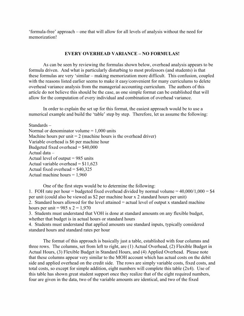
In order to explain the set up for this format, the easiest approach would be to use a numerical example and build the ‘table’ step by step. Therefore, let us assume the following: Standards – Normal or denominator volume = 1,000 units Machine hours per unit = 2 (machine hours is the overhead driver) Variable overhead is $6 per machine hour Budgeted fixed overhead = $40,000 Actual data – Actual level of output = 985 units Actual variable overhead = $11,623 Actual fixed overhead = $40,325 Actual machine hours = 1,960
One of the first steps would be to determine the following: 1. FOH rate per hour = budgeted fixed overhead divided by normal volume = 40,000/1,000 = $4 per unit (could also be viewed as $2 per machine hour x 2 standard hours per unit) 2. Standard hours allowed for the level attained = actual level of output x standard machine hours per unit = 985 x 2 = 1,970 3. Students must understand that VOH is done at standard amounts on any flexible budget, whether that budget is in actual hours or standard hours 4. Students must understand that applied amounts use standard inputs, typically considered standard hours and standard rates per hour
The format of this approach is basically just a table, established with four columns and three rows. The columns, set from left to right, are (1) Actual Overhead, (2) Flexible Budget in Actual Hours, (3) Flexible Budget in Standard Hours, and (4) Applied Overhead. Please note that these columns appear very similar to the MOH account which has actual costs on the debit side and applied overhead on the credit side. The rows are simply variable costs, fixed costs, and total costs, so except for simple addition, eight numbers will complete this table (2x4). Use of this table has shown great student support once they realize that of the eight required numbers, four are given in the data, two of the variable amounts are identical, and two of the fixed
amounts are identical. This means the student is only really responsible for computing three amounts! A visual depiction of the table would be as follows, with letters representing the amounts necessary for completion.
Actual Overhead Flexible Budget in Actual Hours
Flexible Budget in Std Hours
Applied Overhead
Variable A C E G Fixed B D F H Total Sum of A+B Sum of C+D Sum of E+F Sum of G+H
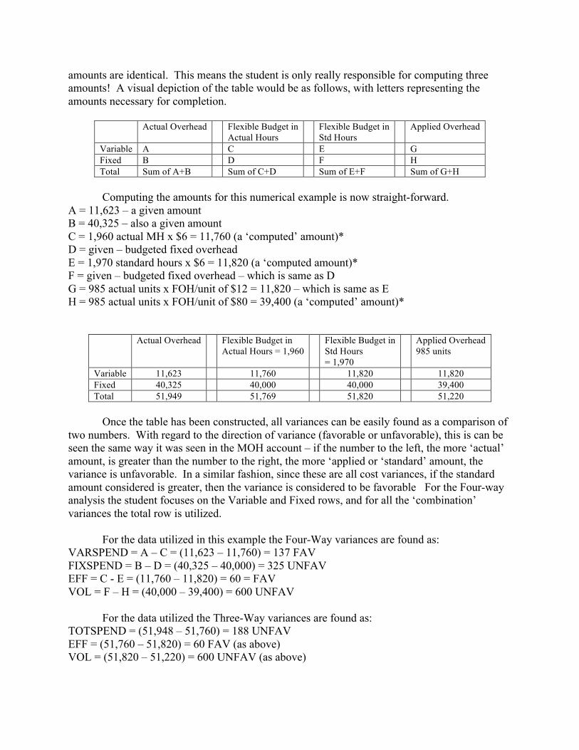
Computing the amounts for this numerical example is now straight-forward.
A = 11,623 – a given amount B = 40,325 – also a given amount C = 1,960 actual MH x $6 = 11,760 (a ‘computed’ amount)* D = given – budgeted fixed overhead E = 1,970 standard hours x $6 = 11,820 (a ‘computed amount)* F = given – budgeted fixed overhead – which is same as D G = 985 actual units x FOH/unit of $12 = 11,820 – which is same as E H = 985 actual units x FOH/unit of $80 = 39,400 (a ‘computed’ amount)*
Actual Overhead Flexible Budget in Actual Hours = 1,960
Flexible Budget in Std Hours = 1,970
Applied Overhead 985 units
Variable 11,623 11,760 11,820 11,820 Fixed 40,325 40,000 40,000 39,400 Total 51,949 51,769 51,820 51,220
Once the table has been constructed, all variances can be easily found as a comparison of
two numbers. With regard to the direction of variance (favorable or unfavorable), this is can be seen the same way it was seen in the MOH account – if the number to the left, the more ‘actual’ amount, is greater than the number to the right, the more ‘applied or ‘standard’ amount, the variance is unfavorable. In a similar fashion, since these are all cost variances, if the standard amount considered is greater, then the variance is considered to be favorable For the Four-way analysis the student focuses on the Variable and Fixed rows, and for all the ‘combination’ variances the total row is utilized.
For the data utilized in this example the Four-Way variances are found as: VARSPEND = A – C = (11,623 – 11,760) = 137 FAV FIXSPEND = B – D = (40,325 – 40,000) = 325 UNFAV EFF = C - E = (11,760 – 11,820) = 60 = FAV VOL = F – H = (40,000 – 39,400) = 600 UNFAV
For the data utilized the Three-Way variances are found as: TOTSPEND = (51,948 – 51,760) = 188 UNFAV EFF = (51,760 – 51,820) = 60 FAV (as above) VOL = (51,820 – 51,220) = 600 UNFAV (as above)
For the data utilized the Two-Way variances are found as: BUDGET = (51,948 – 51,820) = 128 UNFAV VOL = (51,820 – 51,220) = 600 UNFAV (as above)
For the data utilized in this example the One-Way variance is found as: TOTAL = (51,948 – 51,220) = 728 UNFAV
Please note that as the various ways or levels of overhead variance analysis is considered, they all add back to the same amount – the total overhead variance, which in this case is 728 UNFAV.
SUMMARY
The purpose of this article is quite simple – to make the teaching, learning, and understanding of manufacturing overhead variance analysis simple. Too often this topic is deleted from textbooks or from the curriculum of a managerial accounting course due to an incorrect perception of complexity. Too often faculty and students alike believe that the only way this topic can be covered is with pure memorization and is therefore not an efficient use of class time. Hopefully we have provided you with a new way to view the computation of manufacturing overhead variances, at whatever level you believe to be relevant to your students, and have done so without the use of any formulas!

TEACHING PROCESS COSTING
Ronald R. Rubenfield Associate Professor of Accounting and Taxation
Robert Morris University [email protected]
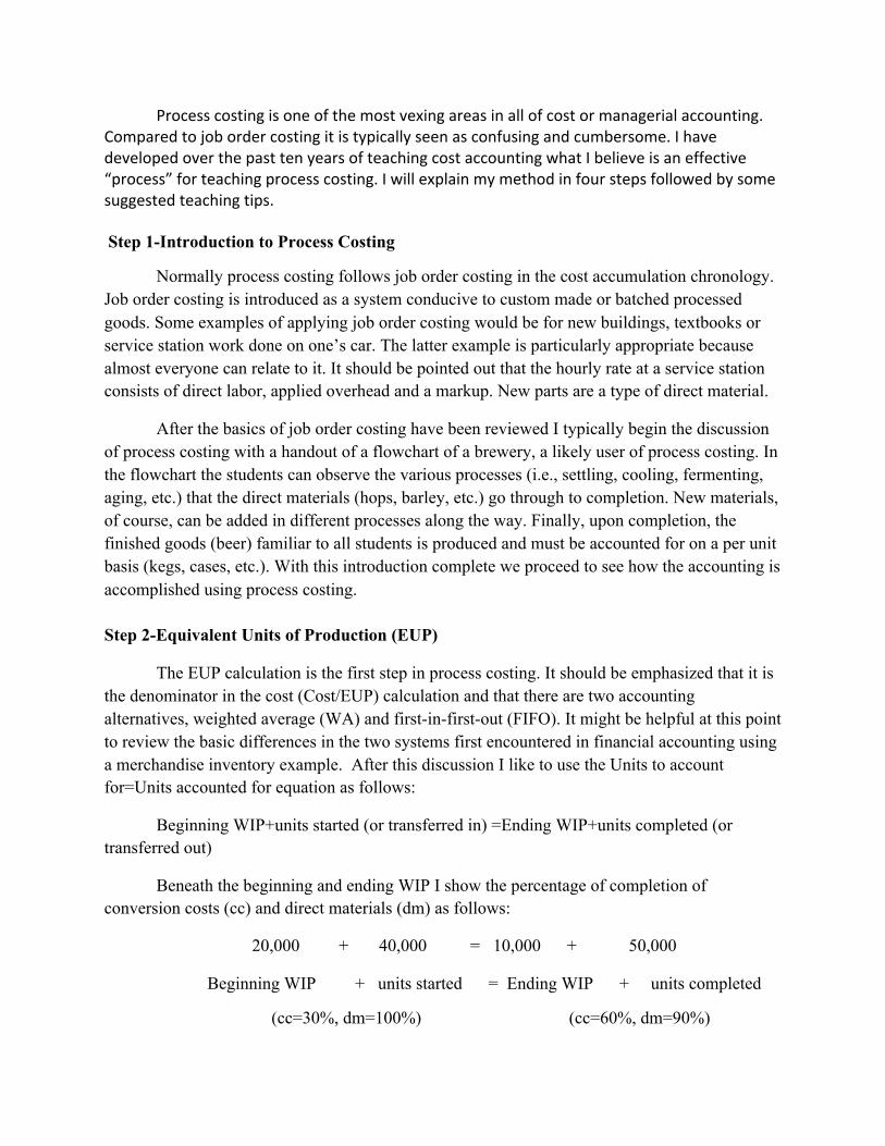
Process costing is one of the most vexing areas in all of cost or managerial accounting. Compared to job order costing it is typically seen as confusing and cumbersome. I have developed over the past ten years of teaching cost accounting what I believe is an effective “process” for teaching process costing. I will explain my method in four steps followed by some suggested teaching tips. Step 1-Introduction to Process Costing
Normally process costing follows job order costing in the cost accumulation chronology. Job order costing is introduced as a system conducive to custom made or batched processed goods. Some examples of applying job order costing would be for new buildings, textbooks or service station work done on one’s car. The latter example is particularly appropriate because almost everyone can relate to it. It should be pointed out that the hourly rate at a service station consists of direct labor, applied overhead and a markup. New parts are a type of direct material.
After the basics of job order costing have been reviewed I typically begin the discussion of process costing with a handout of a flowchart of a brewery, a likely user of process costing. In the flowchart the students can observe the various processes (i.e., settling, cooling, fermenting, aging, etc.) that the direct materials (hops, barley, etc.) go through to completion. New materials, of course, can be added in different processes along the way. Finally, upon completion, the finished goods (beer) familiar to all students is produced and must be accounted for on a per unit basis (kegs, cases, etc.). With this introduction complete we proceed to see how the accounting is accomplished using process costing. Step 2-Equivalent Units of Production (EUP)
The EUP calculation is the first step in process costing. It should be emphasized that it is the denominator in the cost (Cost/EUP) calculation and that there are two accounting alternatives, weighted average (WA) and first-in-first-out (FIFO). It might be helpful at this point to review the basic differences in the two systems first encountered in financial accounting using a merchandise inventory example. After this discussion I like to use the Units to account for=Units accounted for equation as follows:
Beginning WIP+units started (or transferred in) =Ending WIP+units completed (or transferred out)
Beneath the beginning and ending WIP I show the percentage of completion of conversion costs (cc) and direct materials (dm) as follows:
20,000 + 40,000 = 10,000 + 50,000
Beginning WIP + units started = Ending WIP + units completed
(cc=30%, dm=100%) (cc=60%, dm=90%)
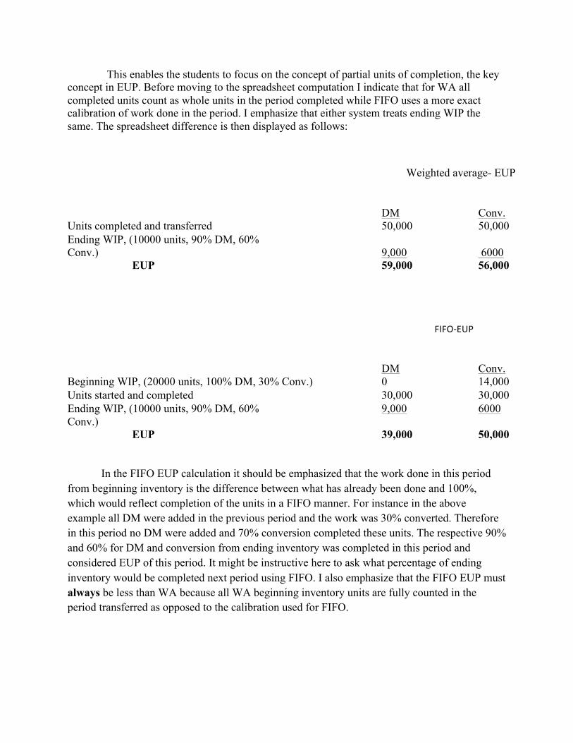
This enables the students to focus on the concept of partial units of completion, the key concept in EUP. Before moving to the spreadsheet computation I indicate that for WA all completed units count as whole units in the period completed while FIFO uses a more exact calibration of work done in the period. I emphasize that either system treats ending WIP the same. The spreadsheet difference is then displayed as follows:
Weighted average- EUP
DM
Conv. Units completed and transferred 50,000 50,000 Ending WIP, (10000 units, 90% DM, 60% Conv.)
9,000
6000
EUP 59,000 56,000
FIFO-‐EUP
DM Conv.
Beginning WIP, (20000 units, 100% DM, 30% Conv.) 0 14,000 Units started and completed 30,000 30,000 Ending WIP, (10000 units, 90% DM, 60% Conv.)
9,000 6000
EUP 39,000 50,000
In the FIFO EUP calculation it should be emphasized that the work done in this period from beginning inventory is the difference between what has already been done and 100%, which would reflect completion of the units in a FIFO manner. For instance in the above example all DM were added in the previous period and the work was 30% converted. Therefore in this period no DM were added and 70% conversion completed these units. The respective 90% and 60% for DM and conversion from ending inventory was completed in this period and considered EUP of this period. It might be instructive here to ask what percentage of ending inventory would be completed next period using FIFO. I also emphasize that the FIFO EUP must always be less than WA because all WA beginning inventory units are fully counted in the period transferred as opposed to the calibration used for FIFO.
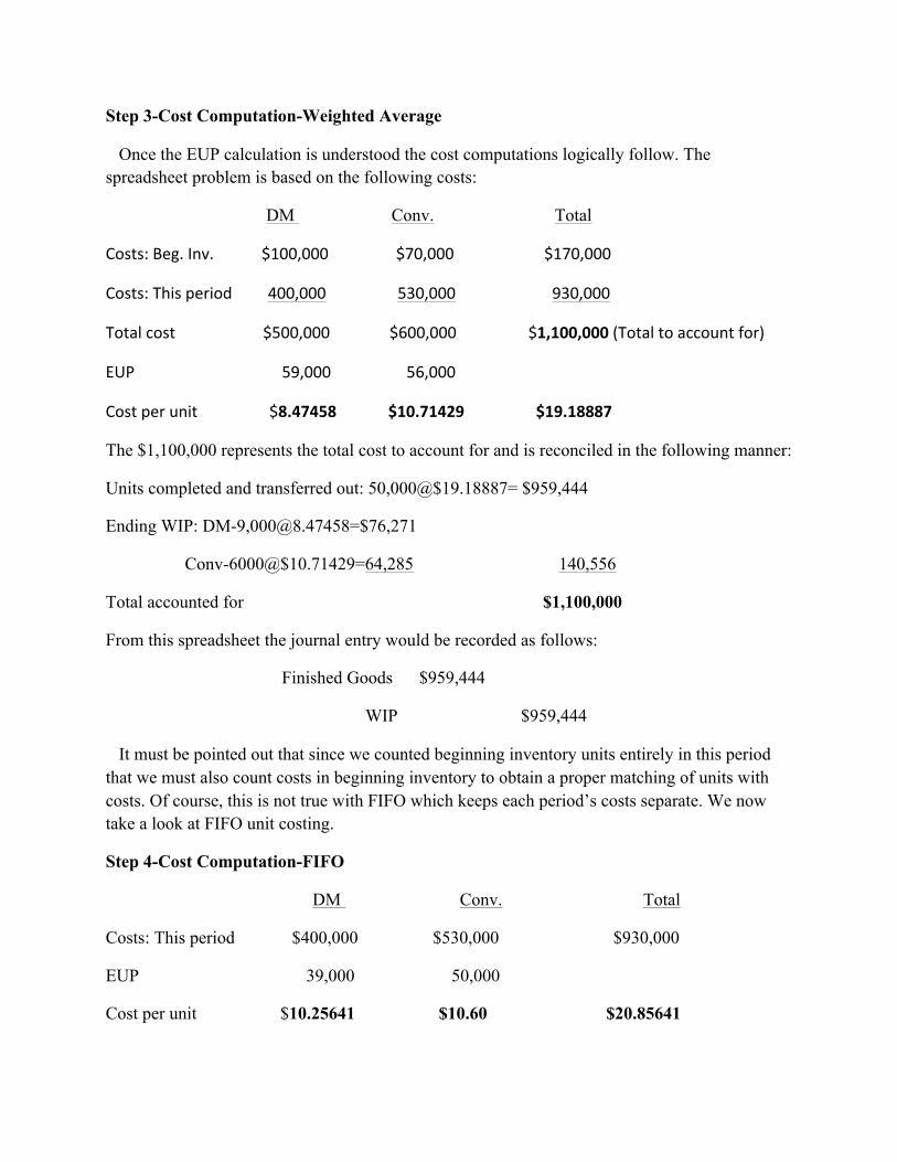
Step 3-Cost Computation-Weighted Average
Once the EUP calculation is understood the cost computations logically follow. The spreadsheet problem is based on the following costs:
DM Conv. Total
Costs: Beg. Inv. $100,000 $70,000 $170,000
Costs: This period 400,000 530,000 930,000
Total cost $500,000 $600,000 $1,100,000 (Total to account for)
EUP 59,000 56,000
Cost per unit $8.47458 $10.71429 $19.18887
The $1,100,000 represents the total cost to account for and is reconciled in the following manner:
Units completed and transferred out: 50,000@$19.18887= $959,444
Ending WIP: DM-9,[email protected]=$76,271
Conv-6000@$10.71429=64,285 140,556
Total accounted for $1,100,000
From this spreadsheet the journal entry would be recorded as follows:
Finished Goods $959,444
WIP $959,444
It must be pointed out that since we counted beginning inventory units entirely in this period that we must also count costs in beginning inventory to obtain a proper matching of units with costs. Of course, this is not true with FIFO which keeps each period’s costs separate. We now take a look at FIFO unit costing.
Step 4-Cost Computation-FIFO
DM Conv. Total
Costs: This period $400,000 $530,000 $930,000
EUP 39,000 50,000
Cost per unit $10.25641 $10.60 $20.85641
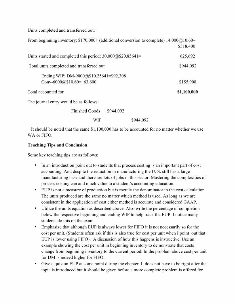
Units completed and transferred out:
From beginning inventory: $170,000+ (additional conversion to complete) 14,[email protected]= $318,400
Units started and completed this period: 30,000@$20.85641= 625,692
Total units completed and transferred out $944,092
Ending WIP: DM-9000@$10.25641=$92,308 Conv-6000@$10.60= 63,600 $155,908
Total accounted for $1,100,000
The journal entry would be as follows:
Finished Goods $944,092
WIP $944,092
It should be noted that the same $1,100,000 has to be accounted for no matter whether we use WA or FIFO.
Teaching Tips and Conclusion
Some key teaching tips are as follows:
• In an introduction point out to students that process costing is an important part of cost accounting. And despite the reduction in manufacturing the U. S. still has a large manufacturing base and there are lots of jobs in this sector. Mastering the complexities of process costing can add much value to a student’s accounting education.
• EUP is not a measure of production but is merely the denominator in the cost calculation. The units produced are the same no matter which method is used. As long as we are consistent in the application of cost either method is accurate and considered GAAP.
• Utilize the units equation as described above. Also write the percentage of completion below the respective beginning and ending WIP to help track the EUP. I notice many students do this on the exam.
• Emphasize that although EUP is always lower for FIFO it is not necessarily so for the cost per unit. (Students often ask if this is also true for cost per unit when I point out that EUP is lower using FIFO). A discussion of how this happens is instructive. Use an example showing the cost per unit in beginning inventory to demonstrate that costs change from beginning inventory to the current period. In the problem above cost per unit for DM is indeed higher for FIFO.
• Give a quiz on EUP at some point during the chapter. It does not have to be right after the topic is introduced but it should be given before a more complete problem is offered for
homework or on the exam. My experience indicates that students benefit tremendously when this is done and do better on the exam as a result.
• Demonstrate that costs to account for must reconcile with costs accounted for in ending WIP and goods transferred out. While this does not always prove the accuracy of the accounting, if it does not reconcile it is certainly incorrect.
• A tricky issue for FIFO EUP is how to compute the started and completed units if it is not given. An easy way to reconcile it would be to subtract the beginning WIP from the units completed (or transferred out) and compare it to the units started (or transferred in) less the ending WIP. In the example above, for instance: 50,000-20,000=40,000-10000 or 30,000.
• For the spreadsheet calculations a good tip is to convey that each method has four basic lines in the calculations. For WA there are two lines for EUP (units transferred out and ending WIP) and two for the cost calculation (beginning WIP and this period’s costs). For FIFO there are three lines for EUP (beginning WIP, units started and completed and ending WIP) and only one (this period’s costs) in the cost calculation.
• Finally, indicate both the financial and managerial accounting uses of process costing. We work toward valuing the inventory and the journal entry as recorded above for financial accounting. For managerial uses the unit cost can be used for control purposes to compare against standards and for decision making such as setting a selling price.
Cost accounting is a required course for most accounting majors. Cost accumulation methods normally receive a great deal of attention in this course. Process costing is the most complex of these methods and normally takes much time and effort to master. Instructors have an opportunity to enhance student learning with effective instruction in this area. I believe that over the years I have developed and applied some teaching techniques that can help in this regard. Hopefully other instructors can benefit from my experience.
USING THE SEILER MODEL FOR STANDARD COSTS VARIANCE ANALYSIS
Carl Brewer Sam Houston State University
Gloria Grayless
Sam Houston State University
Linda Sweeney Sam Houston State University
Contact Author is Carl Brewer E-mail: [email protected] Phone: 936-294-1830
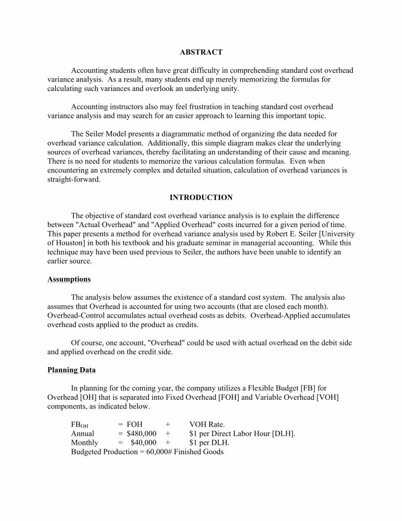
ABSTRACT Accounting students often have great difficulty in comprehending standard cost overhead variance analysis. As a result, many students end up merely memorizing the formulas for calculating such variances and overlook an underlying unity. Accounting instructors also may feel frustration in teaching standard cost overhead variance analysis and may search for an easier approach to learning this important topic. The Seiler Model presents a diagrammatic method of organizing the data needed for overhead variance calculation. Additionally, this simple diagram makes clear the underlying sources of overhead variances, thereby facilitating an understanding of their cause and meaning. There is no need for students to memorize the various calculation formulas. Even when encountering an extremely complex and detailed situation, calculation of overhead variances is straight-forward.
INTRODUCTION The objective of standard cost overhead variance analysis is to explain the difference between "Actual Overhead" and "Applied Overhead" costs incurred for a given period of time. This paper presents a method for overhead variance analysis used by Robert E. Seiler [University of Houston] in both his textbook and his graduate seminar in managerial accounting. While this technique may have been used previous to Seiler, the authors have been unable to identify an earlier source. Assumptions The analysis below assumes the existence of a standard cost system. The analysis also assumes that Overhead is accounted for using two accounts (that are closed each month). Overhead-Control accumulates actual overhead costs as debits. Overhead-Applied accumulates overhead costs applied to the product as credits. Of course, one account, "Overhead" could be used with actual overhead on the debit side and applied overhead on the credit side. Planning Data In planning for the coming year, the company utilizes a Flexible Budget [FB] for Overhead [OH] that is separated into Fixed Overhead [FOH] and Variable Overhead [VOH] components, as indicated below. FBOH = FOH + VOH Rate. Annual = $480,000 + $1 per Direct Labor Hour [DLH]. Monthly = $40,000 + $1 per DLH. Budgeted Production = 60,000# Finished Goods
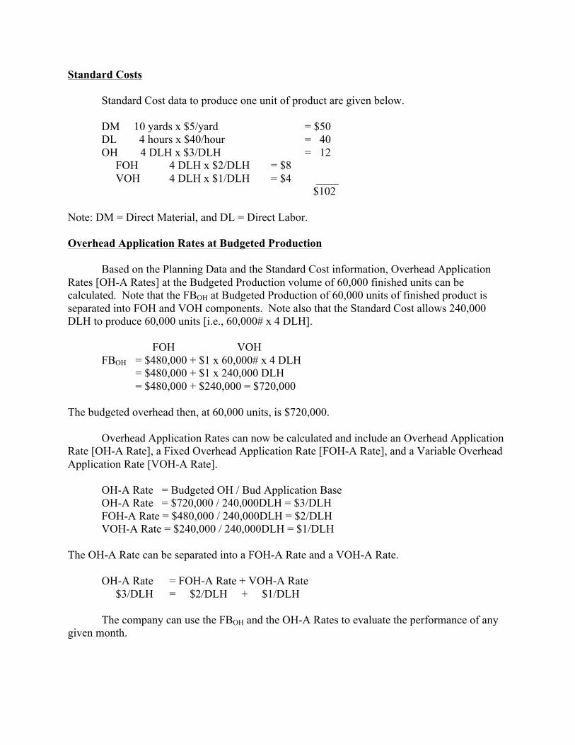
Standard Costs Standard Cost data to produce one unit of product are given below. DM 10 yards x $5/yard = $50 DL 4 hours x $40/hour = 40 OH 4 DLH x $3/DLH = 12 FOH 4 DLH x $2/DLH = $8 VOH 4 DLH x $1/DLH = $4 ____ $102 Note: DM = Direct Material, and DL = Direct Labor. Overhead Application Rates at Budgeted Production Based on the Planning Data and the Standard Cost information, Overhead Application Rates [OH-A Rates] at the Budgeted Production volume of 60,000 finished units can be calculated. Note that the FBOH at Budgeted Production of 60,000 units of finished product is separated into FOH and VOH components. Note also that the Standard Cost allows 240,000 DLH to produce 60,000 units [i.e., 60,000# x 4 DLH]. FOH VOH FBOH = $480,000 + $1 x 60,000# x 4 DLH = $480,000 + $1 x 240,000 DLH = $480,000 + $240,000 = $720,000 The budgeted overhead then, at 60,000 units, is $720,000. Overhead Application Rates can now be calculated and include an Overhead Application Rate [OH-A Rate], a Fixed Overhead Application Rate [FOH-A Rate], and a Variable Overhead Application Rate [VOH-A Rate]. OH-A Rate = Budgeted OH / Bud Application Base OH-A Rate = $720,000 / 240,000DLH = $3/DLH FOH-A Rate = $480,000 / 240,000DLH = $2/DLH VOH-A Rate = $240,000 / 240,000DLH = $1/DLH The OH-A Rate can be separated into a FOH-A Rate and a VOH-A Rate. OH-A Rate = FOH-A Rate + VOH-A Rate $3/DLH = $2/DLH + $1/DLH The company can use the FBOH and the OH-A Rates to evaluate the performance of any given month.
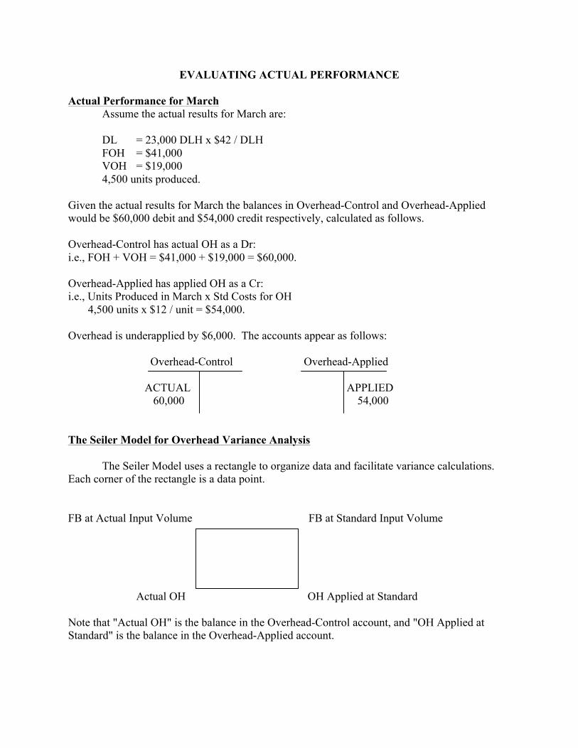
EVALUATING ACTUAL PERFORMANCE Actual Performance for March Assume the actual results for March are: DL = 23,000 DLH x $42 / DLH FOH = $41,000 VOH = $19,000 4,500 units produced. Given the actual results for March the balances in Overhead-Control and Overhead-Applied would be $60,000 debit and $54,000 credit respectively, calculated as follows. Overhead-Control has actual OH as a Dr: i.e., FOH + VOH = $41,000 + $19,000 = $60,000. Overhead-Applied has applied OH as a Cr: i.e., Units Produced in March x Std Costs for OH 4,500 units x $12 / unit = $54,000. Overhead is underapplied by $6,000. The accounts appear as follows: Overhead-Control Overhead-Applied ACTUAL APPLIED 60,000 54,000 The Seiler Model for Overhead Variance Analysis The Seiler Model uses a rectangle to organize data and facilitate variance calculations. Each corner of the rectangle is a data point. FB at Actual Input Volume FB at Standard Input Volume Actual OH OH Applied at Standard Note that "Actual OH" is the balance in the Overhead-Control account, and "OH Applied at Standard" is the balance in the Overhead-Applied account.
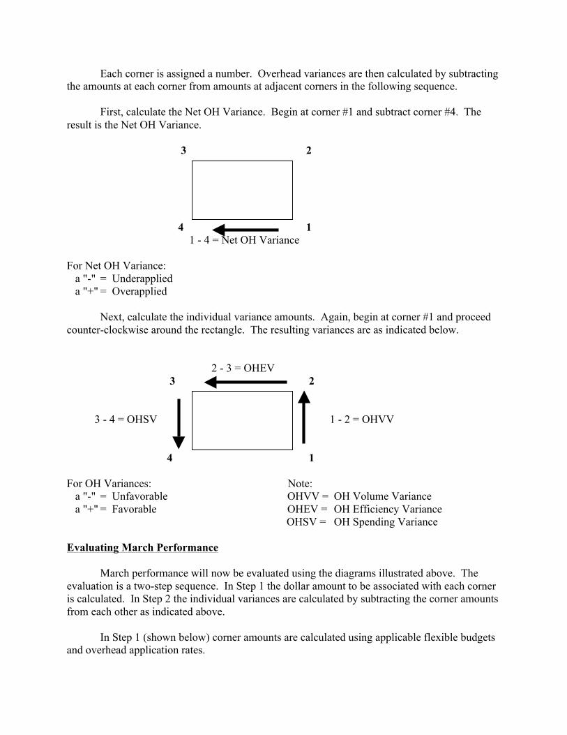
Each corner is assigned a number. Overhead variances are then calculated by subtracting the amounts at each corner from amounts at adjacent corners in the following sequence. First, calculate the Net OH Variance. Begin at corner #1 and subtract corner #4. The result is the Net OH Variance. 3 2 4 1 1 - 4 = Net OH Variance For Net OH Variance: a "-" = Underapplied a "+" = Overapplied Next, calculate the individual variance amounts. Again, begin at corner #1 and proceed counter-clockwise around the rectangle. The resulting variances are as indicated below. 2 - 3 = OHEV 3 2 3 - 4 = OHSV 1 - 2 = OHVV 4 1 For OH Variances: Note: a "-" = Unfavorable OHVV = OH Volume Variance a "+" = Favorable OHEV = OH Efficiency Variance OHSV = OH Spending Variance Evaluating March Performance March performance will now be evaluated using the diagrams illustrated above. The evaluation is a two-step sequence. In Step 1 the dollar amount to be associated with each corner is calculated. In Step 2 the individual variances are calculated by subtracting the corner amounts from each other as indicated above. In Step 1 (shown below) corner amounts are calculated using applicable flexible budgets and overhead application rates.
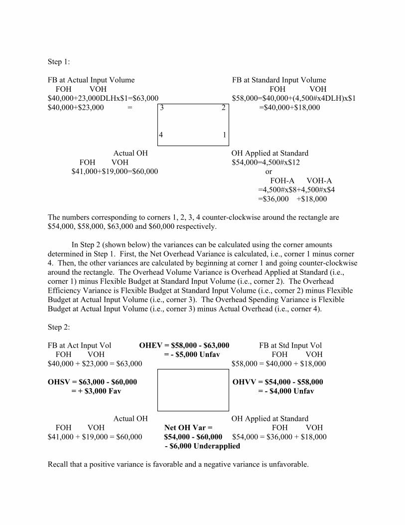
Step 1: FB at Actual Input Volume FB at Standard Input Volume FOH VOH FOH VOH $40,000+23,000DLHx$1=$63,000 $58,000=$40,000+(4,500#x4DLH)x$1 $40,000+$23,000 = 3 2 =$40,000+$18,000 4 1 Actual OH OH Applied at Standard FOH VOH $54,000=4,500#x$12 $41,000+$19,000=$60,000 or FOH-A VOH-A =4,500#x$8+4,500#x$4 =$36,000 +$18,000 The numbers corresponding to corners 1, 2, 3, 4 counter-clockwise around the rectangle are $54,000, $58,000, $63,000 and $60,000 respectively. In Step 2 (shown below) the variances can be calculated using the corner amounts determined in Step 1. First, the Net Overhead Variance is calculated, i.e., corner 1 minus corner 4. Then, the other variances are calculated by beginning at corner 1 and going counter-clockwise around the rectangle. The Overhead Volume Variance is Overhead Applied at Standard (i.e., corner 1) minus Flexible Budget at Standard Input Volume (i.e., corner 2). The Overhead Efficiency Variance is Flexible Budget at Standard Input Volume (i.e., corner 2) minus Flexible Budget at Actual Input Volume (i.e., corner 3). The Overhead Spending Variance is Flexible Budget at Actual Input Volume (i.e., corner 3) minus Actual Overhead (i.e., corner 4). Step 2: FB at Act Input Vol OHEV = $58,000 - $63,000 FB at Std Input Vol FOH VOH = - $5,000 Unfav FOH VOH $40,000 + $23,000 = $63,000 $58,000 = $40,000 + $18,000 OHSV = $63,000 - $60,000 OHVV = $54,000 - $58,000 = + $3,000 Fav = - $4,000 Unfav Actual OH OH Applied at Standard FOH VOH Net OH Var = FOH VOH $41,000 + $19,000 = $60,000 $54,000 - $60,000 $54,000 = $36,000 + $18,000 - $6,000 Underapplied Recall that a positive variance is favorable and a negative variance is unfavorable.
CLOSING COMMENTS While the Seiler Method provides an easy way to calculate overhead variances, it also highlights the causes underlying the variances. Comparing the numbers comprising the Overhead Volume Variance discloses the amounts at corner #1 and corner #2 have the same variable overhead amounts indicating the Overhead Volume Variance is strictly based on fixed overhead differences. Similarly, corners #2 and #3 differ only in their variable overhead amounts. Fixed overhead is the same indicating the Overhead Efficiency Variance is based only on variable overhead. Corners #3 and #4 differ in both fixed overhead and variable overhead amounts, indicating the Overhead Spending Variance is comprised of both a fixed overhead component and a variable overhead component. Indeed, a Fixed Overhead Spending Variance and a Variable Overhead Spending Variance could easily be calculated. Both the Overhead Efficiency Variance and the Overhead Spending Variance are controllable by manufacturing production. An Overhead Controllable Variance, sometimes called an Overhead Budget Variance, can be calculated by subtracting corner #4 from corner #2, i.e., #2 minus #4.
REFERENCES Seiler, R.E. 1971. Accounting Principles for Management: An Introduction. Merrill. Seiler, R.E. 1977. Overhead Variance Analysis - Classroom presentation. Graduate Seminar in
Managerial Accounting, University of Houston.