Embed Size (px)
Citation preview

Accounting Standards, Earnings Management,
and Earnings Quality
Ralf Ewert
and
Alfred Wagenhofer
University of Graz
We thank Wolfgang Ballwieser (discussant), Anna Boisits, Judson Caskey (discussant),
Frank Gigler, Mirko Heinle, Rick Lambert, Stefan Schantl, Marco Trombetta
(discussant), and participants at the Ausschuss Unternehmensrechnung of the Verein für
Socialpolitik, EAA Congress 2013, Accounting Research Workshop at the University of
Basel, Tel Aviv International Conference in Accounting, and workshop participants at
the University of Minnesota and at the University of Pennsylvania for helpful
comments.
Ralf Ewert
University of Graz, Universitaetsstrasse 15, A-8010 Graz, Austria
Tel.: +43 (316) 380 7168, Email: [email protected]
Alfred Wagenhofer
University of Graz, Universitaetsstrasse 15, A-8010 Graz, Austria
Tel.: +43 (316) 380 3500, Email: [email protected]
November 2013

1
Accounting Standards, Earnings Management,
and Earnings Quality
This paper examines how the characteristics of accounting systems and management
incentives interact and collectively determine financial reporting quality. We develop a
rational expectations equilibrium model that features a steady-state firm with investments,
financial and non-financial information, and earnings management. Our measure of earnings
quality is the equilibrium information content of reported earnings. We study effects on
earnings quality by varying the accruals, the precision of base earnings and private non-
financial information, the cost of earnings management, and operating risk. The analysis
confirms some intuitive results, such as that earnings quality increases in the precision of
earnings and non-financial information. However, we also find counter-intuitive results, such
as that an accounting standard that unambiguously provides more information early can
reduce earnings quality. Since the equilibrium market reaction is akin to value relevance
measures, we study how these measures trace the changes in earnings quality. We show that
the earnings response coefficient is more closely related to earnings quality than the
correlation of a price-earnings regression.
Keywords: Earnings quality; earnings management; accounting standards; value relevance;
earnings response coefficient.
JEL classification: D80; G12; G14; M41; M43.
2
1. Introduction
Earnings quality is an important characteristic of financial reporting systems. Most
recent regulatory changes in accounting standards, auditing, and corporate governance have
been motivated by attempts to increase transparency of financial reporting. Earnings quality is
also used in many empirical studies to examine changes in earnings characteristics over time,
to assess the effects of changes in accounting standards and the institutional environment, to
compare financial reporting across countries, and to measure market price and return effects
of firms exhibiting different earnings quality. Dechow, Ge, and Schrand (2010) provide a
broad survey of this literature.
Despite this great interest, there is little theory examining the consequences of a change
in accounting standards and the institutional setting on earnings quality or, more generally,
financial reporting quality. One reason is that earnings quality is an elusive notion that is
being used to capture a variety of attributes. Another is that many regulatory initiatives and
empirical studies are based on intuitive reasoning such as, for example, that an earlier
recognition of components of future cash flows or a reduction of the discretion for earnings
management increase earnings quality. This paper provides a theoretical analysis of the
effects of a variation of accounting system characteristics on earnings quality, where earnings
quality is the information content carried in reported earnings for pricing the firm. We show
that several, a priori intuitively plausible, relationships are not warranted and provide reasons
why and when this is the case.
We develop a simple stochastic steady-state model of a firm that invests in two-period
projects in every period. An accounting system recognizes a portion of the future expected
cash flows early, but with noise. The model is rich enough to give rise to investment,
depreciation, working capital accruals, and earnings. The manager privately observes the
accounting signal and obtains additional non-financial information that is not recognized in
the financial reporting system. We allow for earnings management through which the
manager can issue an earnings report to the capital market that includes the accounting signal
with bias. Since the manager conditions the bias on all available information, including the

3
non-financial information, reported earnings include two pieces of information, information
from the accounting system and the non-financial information. The total information content
of reported earnings depends on the characteristics of the information and on the incentives of
the manager. We examine price, earnings, and smoothing incentives and show that
particularly smoothing leads to two distinct effects which affect earnings quality in opposite
directions: On one hand, to smooth earnings the manager considers current as well as future
earnings, so that the resulting bias incorporates the manager’s private information and this
generally improves earnings quality. On the other hand, the manager’s ability to smooth is
affected by the smoothing inherent in the accounting system, so that in equilibrium a more
informative accounting system can actually reduce earnings quality.
We establish a unique linear rational expectations equilibrium and describe the
equilibrium earnings management and market price reaction. Earnings management exhibits a
period-specific bias and forward and backward smoothing. In equilibrium, investors are able
to make inferences about this information and use it in pricing the firm. To do so, they use
information in reported earnings as well as balance sheet and cash flow information. Earnings
quality is defined in the model in terms of the information content of reported earnings in
equilibrium.
This economic setting is useful to study the effects of variations in accounting standards
and the institutional environment on earnings quality. The effects of such variations are not
straightforward because the equilibrium implies a subtle interrelationship between the effect
on the accounting system and the earnings management bias. The characteristics
endogenously influence the weights with which the manager’s information is integrated in
reported earnings, which again affects the amount of information investors can infer from the
earnings report about the manager’s information.
The characteristics of the accounting system we consider are the degree to which it
reports components of the projects’ expected cash flows that realize before the cash flows
obtain, and how precise this early recognition is. We find that a greater portion of anticipated
future cash flows embedded in earnings does not always increase earnings quality. The reason

4
is that it dampens the inclusion of non-financial information in the bias, which can dominate
the increase in the information content of the accounting signal. Next, we establish that an
increase in the precision of the accounting system and the private information always
increases earnings quality. However, an increase in the cost of earnings management (e.g.,
less discretion, higher audit and enforcement quality) reduces earnings quality. This result
obtains because a higher cost reduces earnings management in equilibrium, which does not
improve earnings quality as investors correctly undo it on average, but is harmful as it lowers
the weight with which the manager’s non-financial information enters reported earnings.
We also provide insights into the effect of a change in the amount of operative (cash
flow) risk that is captured by the accounting system or by the manager’s non-financial
information relative to the total risk. A higher operative risk of cash flow components for
which information becomes available generally increases earnings quality; however, we
identify circumstances in which the converse happens. Again, the reason is the interaction of
the equilibrium weights of accounting and non-financial information in the earnings report.
Finally, we examine how value relevance measures that are used as empirical proxies
for earnings quality react to changes in our earnings quality benchmark. Value relevance is
closely related to our rational expectations capital market setting, as it measures the price
changes based on reported earnings. We study the earnings response coefficient and the
correlation of a price-earnings regression and show how they are related to earnings quality.
The main finding is that the earnings response coefficient is closely related to earnings
quality, whereas the correlation measure does not capture earnings quality well. Still, even the
earnings response coefficient is not a perfect proxy, mainly because the market is able to rely
on more information than earnings in forming the price. We also show that the behavior of the
proxies differs whether they are used in a study that compares two equilibria with different
accounting characteristics or that assesses the effects of a change in the characteristics in the
same setting over time.
There are several caveats that we should note at the outset. For simplicity, we do not
model a full agency model with optimal compensation, but exogenously assume management

5
incentives to show that particularly earnings smoothing can have detrimental effects on
earnings quality. The model does not capture productive decisions by the manager, apart from
earnings management (which can be interpreted as real activities to shift earnings across
periods) and shows that even in a pure exchange economy a negative value of more
informative standards can occur. The technical requirements of the equilibrium does not allow
us to model many aspects of accounting standards, such as asymmetric information
introduced by conservatism. Presumably, extending the model structure would result in even
more frictions than those we identify.
There is little theoretical literature that directly addresses earnings quality and its
measures, although a notion of earnings quality is embedded in many analytical studies.
Closely related is Fischer and Verrecchia (2000) who study the value relevance of an earnings
report in equilibrium and find that informativeness increases in the cost of bias. Unlike the
present paper they do not specifically model an accounting structure with accruals and
consider a one-period setting. Sankar and Subrahmanyam (2001) study a two-period model
with a risk averse manager with a time-additive utility function where smoothing results from
the manager’s desire to smooth consumption. They find that allowing for earnings
management improves the information in the capital market because the bias allows the
manager to incorporate private value relevant information early. Dye and Sridhar (2004) study
relevance and reliability of accounting information and model the accountant as the
gatekeeper to trade off these two characteristics in a capital market equilibrium. In their
model, the accountant aggregates the two pieces of information, whereas in the present model
the aggregation arises in the market under rational expectations.
Closest to the present paper is Ewert and Wagenhofer (2013). They study a two-period
rational expectations equilibrium model and examine a variation of accounting, incentive, and
risk parameters on earnings quality. Further, they study value relevance, persistence,
predictability, smoothness, and discretionary accruals in this setting. Different from their
setting, we study a steady state model and exploit the natural accounting structure with
depreciation and working capital accruals. Some of the results of the present paper mirror

6
those in Ewert and Wagenhofer (2013), but the main focus is on the interaction of accounting
standards and incentives.1 Marinovic (2013) examines earnings management and capital
market reactions when there is uncertainty whether the manager can bias the earnings report.
He establishes a mixed-strategy equilibrium, in which price volatility around earnings
announcements and persistence are useful measures, whereas predictability and smoothness
behave non-monotonically in the information content of reported earnings. Fischer and
Stocken (2004) examine how varying a speculator’s information affects earnings management
incentives. They define earnings quality as squared difference between reported and
fundamental earnings and find that the effect depends on whether the speculator’s information
complements or substitutes for earnings.
These models focus on the decision usefulness of accounting earnings in a capital
market equilibrium. Other papers study aspects of earnings quality in agency models, e.g.,
Christensen, Feltham, and Şabac (2005) and Christensen, Frimor, and Şabac (2013), and
Drymiotes and Hemmer (2013). These papers generally find that value relevance metrics
often do not capture underlying economic effects, which is in spirit similar to our results,
although the economic forces are very different.
The rest of the paper is organized as follows: In the next section we set up the model
with the investment projects, the accounting system, earnings management incentives, and the
structure and information content of the financial reports. Section 3 establishes the rational
expectations equilibrium and describes the properties of the equilibrium earnings report and
market pricing mechanism. The main analysis of earnings quality and its determining factors
is included in section 4. Section 5 considers value relevance and how the two value relevance
proxies trace earnings quality. Finally, section 6 concludes and discusses potential extensions.
1 Christensen and Frimor (2007) study the interaction between accounting information and other information in a
capital market setting. Similar in spirit to our paper, they find that more information may be undesirable because
it affects the weights with which they are enter the pricing mechanism.

7
2. The Model
Firms are regularly operative over an open time-horizon; they generate cash flows,
realize new projects and terminate existing projects in each period; they operate an accounting
system that allocates past and anticipated cash flows over time by means of accruals and the
capitalization of assets and liabilities; and the firm’s management changes after some periods.
Earnings quality can only be analyzed in the context of these factors, and we capture these
essential aspects in a parsimonious way.
Investment projects
We model a simple ongoing firm, which obtains an investment opportunity in each
period. All projects are structurally equal.2 Each project requires a certain investment cost I >
0 at the beginning of a period and yields a risky operating cash flow x at the end of the
second period. This situation is descriptive of construction contracts or other contracts in
which cash flows and the underlying operations occur at different times. The main results
would continue to hold for projects with more cash flows at different times. The cash flow x
is normally distributed with a mean and the expected net present value of the project is
strictly positive,
2 0NPV I ,
where (0, 1] denotes the discount factor. Hence, each investment project that arises will
be implemented; for simplicity, we abstract from non-trivial investment decisions and ignore
potential abandonment decisions. To eliminate effects of financing decisions we assume that
the firm distributes excess cash flows and raises equity if cash flows fall short of investment
requirements.
The cash flow x consists of three operating risk factors,
x (1)
2 It would be possible to assume different projects, e.g., projects with a growth rate that is less than the discount
rate. However, the additional insights gained would be low.

8
which are normally and independently distributed with zero mean and variances
2 2 2, and . For example, it describes a situation in which the risk factors realize at
different times. The cash flow structure of the projects is common knowledge. The investment
I and the cash flow x are publicly observable, whereas the individual stochastic components
of x are not.
Accounting system
The firm operates an accounting system that provides signals about the future cash
flows of each active project to the manager. We distinguish between information that is
recognized in the financial statements and other, information that we label non-financial. We
assume that the recognized accounting earnings 1y are informative about one component of
the uncertain future cash flow, , in the following way:
1y k n . (2)
This formulation captures two important characteristics of an accounting system.3 First, the
parameter k (0, 1] determines the portion of the future cash flow caused by the factor . For
example, k = 1 implies that 1y fully contains ; k = 0 prohibits early recognition of any future
cash flows and would lead to an uninformative accounting system, which is the reason that we
exclude it.4 Second, the accounting system imperfectly traces in that the signal is noisy,
where the noise n is independent of the accrual k and normally distributed with zero mean
and variance 2
n . Lower 2
n indicates that the accounting system is more precise.5
3 In line with most accounting standards, we assume that the expected profit is recognized in the second
period. Since carries no information to investors, this assumption is not restrictive. Moreover, in our steady
state structure this assumption is without loss of generality even for reported earnings, as there are always two
active projects in each period, so that the sum of the individual accounting signals contains of one project.
4 It should be noted that varying the degree of inclusion of also affects the overall precision of the manager’s
private information because it is “real” variance in contrast to the constant accounting noise.
5 An alternative assumption is 1 ( )y k n , so higher k increases both the information about and the noise in
1y . A standard setter would then trade off these two effects. We do not use this assumption in order to separate
information content and precision.

9
For example, suppose the project is a long-term contract, then k is the portion of the
contracted revenue or gain from work completed in period t. Alternatively, k may be the
costs incurred or the sold products or services from the project which is paid later. The
accounting signal 1y is a typical accrual in the accounting system, as it recognizes a portion of
future expected cash flows early. We assume the accounting system is exogenously given,
e.g., by an accounting standard, and we vary the information content by changing k and 2
n to
examine their impact on earnings quality. Note that both k and 2
n affect the variance of 1y ,
albeit in an economically different way, as we show later.
In the second period the cash flow x realizes. The accounting system generates the
signal
2 1 (1 ) .y x y k n
The accounting system obeys the clean surplus condition, which requires that the total
accounting earnings are equal to total cash flows, i.e., for each project 1 2y y x .
The investment cost I is depreciated at commonly known (or observable) rates; periodic
depreciation is d1 and d2, where I = d1 + d2.6 Thus, we distinguish working capital accruals ty
and other accruals (depreciation dt).
The manager obtains additional private information, referred to as non-financial
information. The source of the information may be the internal management accounting
system or other external information. This information is not recognized in the financial
statements and cannot credibly be communicated by the manager. We model the non-financial
information by a signal
z u
about the cash flow component with noise u , which is normally distributed with zero
mean and variance 2
u . All random variables are mutually independent. Assuming that the
6 Since d1 and d2 are common knowledge, they carry no incremental information, but are needed to capture the
accounting depiction of the investment outlay.

10
internal accounting system also traces non-financial information, we treat 2
u as another
characteristic of the accounting system.
Neither the accounting system nor other sources of the manager provide information
about the third cash flow component , so 2
is the residual risk of the project’s cash flow.
Thus, the accounting system is characterized by 2 2( , , )n uk which is common knowledge.
We allow the manager to influence the earnings from the accounting system by
introducing a bias so that reported earnings can deviate from the the original accounting
earnings. In the first period of a project, the manager chooses a bias b (where b can be
positive or negative), which is reversed in the second period of a project. The bias can be a
result of applying a particular revenue recognition or cost allocation procedure or of
exercising discretion in the estimation of future revenues and costs or may consist of real
activities that shift income from one period to the other. While the literature often views the
introduction of a bias as undesirable earnings management that destroys information, our
formulation also comprises the possibility that a bias carries more information (in our model
about the manager’s private non-financial information).
In sum, the reported earnings for each project in period 1 and 2 are
1 1 1 1
2 2 2 21 ,
m y d b k n d b
m y d b k n d b
(3)
where 1 2m m x I .
Manager’s incentives
The choice of the bias b depends on the manager’s private information and incentives
for bias. At the time the manager decides on b, she has available the accounting earnings y
from the projects in the respective period and the non-financial information z of the new
project. Therefore, b = b(y, z). We assume a manager is hired and works for two periods, then

11
leaves the firm and is replaced by a new manager with the same characteristics.7 Figure 1
summarizes the sequence of events.
[Insert Figure 1 about here]
We do not explicitly model reasons for specific management incentives, but assume
incentives of managers that are most common in practice. In particular, survey results by
Graham, Harvey and Rajgopal (2005) indicate that the overwhelming majority of surveyed
managers have objectives that are tied to market prices and to earnings8 and include a desire
to smooth earnings over time.9 Since we are interested in the interaction between accounting
standards and management incentives, we include all of these possible incentives. In
particular, we assume risk neutral managers and consider short-term market price, reported
earnings, smoothing reported earnings over the two periods, and that earnings management is
privately costly to the manager. In the first period, the manager has the following utility
function:
22 1
1 1 1 1 1[( ) ]2
t t t
bU p P g M s M M r . (4)
In the second period, the utility function is
2
22 2 2 2 1
2t
bU p P g M r . (5)
7 Longer tenure would significantly increase the complexity of the analysis because each bias choice must take
into account subsequent biases. Since period 2 is the ending period, we view period 1 as a representative period
for our analysis.
8 Possible reasons for the optimality of incentive systems combining market price and accounting numbers can
be found in Dutta and Reichelstein (2005) and Dutta (2007).
9 Dichev et al. (2013) report that hitting earnings benchmarks, influencing executive compensation, and
smoothing earnings are among the most frequent motivations for earnings management.

12
The number indexes j = 1, 2 indicate the tenure of the manager. For simplicity, we
assume a zero discount rate for the manager’s utility.
First, the manager’ utility can be based on the respective contemporaneous market
prices of the firm Pt (determined in the rational expectations equilibrium), which enter with
weights p1 and p2. For example, the manager is evaluated on market price, holds stock
(ignoring bankruptcy), or plans to raise external capital and wants to boost the market price.
For most of the analysis, we assume pj > 0 in explaining the results, but the analysis is not
restricted to a positive pj.
Second, the manager’s utility can be based on reported period earnings, where Mt is the
total of the projects’ individual earnings reports (which we describe later). The weights are g1
and g2. This interest may arise from a compensation scheme that depends on reported
earnings, earnings targets the manager wants to reach, from political cost considerations or
covenants that depend on earnings.
Third, the manager may be interested in smoothing reported earnings over the two
periods of tenure. There are several reasons that smoothing abounds. One reason is risk
aversion of a manager, but it can exist under risk neutrality to reduce earnings volatility
(Trueman and Titman 1988) or to improve the market’s inference of the report precision
(Kirschenheiter and Melumad 2002); it can be the result of an optimal contract (Dye 1988,
Demski 1998) or it can emerge from the existence of earnings targets, career concerns, and
the like.10 We formalize smoothing in (4) by the expectation of the squared differences
between first-period earnings and second-period earnings, weighted with s ≥ 0. While
smoothing is forward-looking and seeks to smooth current and expected future reported
earnings, our subsequent analysis shows that backward smoothing occurs as well, because the
manager “inherits” earnings from a project invested by the predecessor. At the end of the
second period, the manager leaves the firm and does not care about smoothing second-period
10 De Jong et al. (2012) report that even analysts recognize positive consequences of smooth earnings, although
they dislike earnings smoothing if it reduces transparency.

13
earnings.11 Thus, there is a “horizon effect” in that the manager is interested in a smooth
earnings stream only as long as she operates the current firm, but not so when leaving the
firm.
Finally, the manager bears a cost from undertaking earnings management. In line with
many papers on earnings management,12 we assume that this cost is convex in the bias bj (the
manager can bias earnings in each period j) and scaled by a weight r ≥ 0. The cost captures
personal discomfort and other costs of earnings management, and it is affected by accounting
standards and institutional factors, such as auditing and enforcement effectiveness, liability
risk, and corporate governance provisions. We assume that the cost occurs in (or can be
attributed to) the period in which the manager biases the earnings report, but not in
subsequent periods in which the bias reverses. Subsequently, we use bias and earnings
management interchangeably because the manager has an incentive to manage earnings rather
than directly providing private information to the market. In equilibrium the bias is in fact
informative, so allowing for “earnings management” turns out to be desirable.
We assume the weights are exogenous constants and common knowledge.13 The use of
four weights (rather than three, which would be sufficient to capture the substitution rates
between the components) allows us to identify the effects of each individual component
separately in equilibrium.
Financial reports
Next we describe the financial reports in the steady state setting. The financial report
consists of aggregate reported earnings, the two projects’ cash flows and the net assets. Since
we do not explicitly track cash flows from financing, the net assets are not necessarily equal
11 Huson et al. (2012) provide empirical evidence that compensation committees adjust the weights in the
variable compensation in the final year of a CEO to counter the CEO’s greater incentives for earnings-increasing
manipulation.
12 See, e.g., Fischer and Verrecchia (2000), Stocken and Verrecchia (2004), Ewert and Wagenhofer (2005).
13 Thus, we exclude private information about the weights. For an analysis of an uncertain market price weight p
see Fischer and Verrecchia (2000).

14
to the accumulated differences between reported earnings and cash flows. To distinguish
between projects, we index projects that start at the beginning of period t with t.14 In each
period there are two active projects, one that is started and the other that ends. Since the
situation is similar for all managers, we choose a representative manager and examine the two
periods of her tenure (j = 1, 2) in detail, which are the periods t and t+1.
[Insert Figure 2 about here]
As depicted in Figure 2, reported earnings in each period are the aggregate individual
earnings of the two active projects. These are for the current manager’s tenure:
1 2 1
2 2 2 1 1 1
2 2 1 1
( 1) ( )
( 1) ( )
( 1) ( ) .
M m t m t
y t d b y t d b
y t b y t b I
(6)
2 2 1
2 2 1 1 1 2
2 1 1 2
( ) ( 1)
( ) ( 1)
( ) ( 1) .
M m t m t
y t d b y t d b
y t b y t b I
(7)
The manager „inherits“ earnings m2(t–1) from the previous manager, including the bias
b2 which the outgoing manager had chosen. The current manager selects the bias b1 for the
recent project, which reverses in the second period. Moreover, the current manager chooses a
bias b2 in the second period. While this b2 in expression (7) is formally different from that in
expression (6), it is of the same amount because the managers are similar.
Although the earnings components from two projects are reported in aggregate, the
information in the financial statements allows sophisticated investors to disentangle them and,
therefore, investors use the information about the two active projects separately when
determining the value of the firm. Since I is common knowledge, m1(t) can be calculated from
the cash flows x(t–1) – I and the end-of-period net assets,
14 To facilitate readability, we do not index the random cash flow components if it is not confusing.

15
1 1 1 1
Carrying amontCash from Working capitalof current projectending project accruals of
current project
( 1) ( ) ( 1) ( ) .x t I m t x t I d y t b
Define W1(t) = y1(t) + b1 as working capital accruals of the project starting in period t in the
first period of the manager’s tenure. Since project t–1 ends in period t, the market observes
x(t–1), so W1(t) is the component that carries all available information for valuing the firm at
the end of period t.
The cum dividend market price of the firm at t in the first period of the manager’s
tenure is
1
11
1t tP x t x t W t NPV
(8)
where is the market discount factor and the last term is the net present value of an infinite
period of future projects. Since projects are equal, the net present value does not depend on
current projects and information. The market price at the end of t+1 is
1 1 2
11 1
1t tP x t x t W t NPV
. (9)
where 2 1 2( 1) ( 1)W t y t b and where the manager selects b2 in the last period of her
tenure. Thus, the market uses the reported earnings (and, equivalently, accruals) to update its
beliefs about the future cash flows of the project started in the respective period. As we show
in the subsequent analysis, accounting information from the current and the prior year is a
sufficient statistic for investors to infer pricing information.
3. Equilibrium
A rational expectations equilibrium consists of a reporting strategy by the manager (the
bias) and a capital market pricing mechanism that correctly infers the information contained
in the earnings report on average. Each of these strategies is an optimal response based on the
conjectures of the other player’s strategy. In equilibrium these conjectures are fulfilled. In line

16
with much of the rational expectations equilibrium literature we restrict attention to linear
equilibria.15
The manager maximizes her expected utility by choosing b contingent on her
information set and her conjecture about the market price contingent on the earnings report,
which are16
ˆˆ ˆt t t tP W
where hats on variables indicate conjectures and Wt stands for the information variable in
period t.
Starting backwards with the second period, the manager’s utility is
2
22 2 2 2 2 2 2( 1)
2
rbU p W t g M . (10)
Since W2(t+1) = y1(t+1) + b2, the first-order condition determines the optimal accounting bias:
2 2 22
ˆp gb
r
. (11)
While b2 can be a function of y1(t+1) and z(t+1), the optimal bias is a constant that is
independent of that information. This is a consequence of the fact that the manager’s utility
function is common knowledge, that the formal structure is linear, and that the manager
leaves the firm at the end of this period.
In the first period of tenure, the manager selects the bias b1 by maximizing the first-
period utility U1 and the expected second-period utility U2, given the sequentially rational bias
*
2b . The first-period utility is
15 See, e.g., Fischer and Verrecchia (2000). Guttman, Kadan, and Kandel (2006) prove the existence of equilibria
with partial pooling. Einhorn and Ziv (2012) show that such equilibria do not survive the D1 criterion of Cho
and Kreps (1987).
16 In this equation, we show the market discount factor separately, so that β is only driven by the market’s
revision of expectations.
17
22
1 1 1 1 1 1 1
1 1 1 1 1 2 1 1
2
22 2 22 1 2 1 1 1
, ( )2
ˆˆ Var ( ) ( 1) ( ), ( )
ˆ( ) ( ), ( ) 2 ( 1) ( ) 2
2
t t t
t
rU p P g M s M M y t z t b
p W t g M s y t y t y t z t
p g rs y t y t z t y t y t b b
r
(12)
where the second expression results from substituting for Mt and 1tM from (6) and (7), that is
2 2 21 2 1 2 1 1
ˆ( ) ( 1) ( 1) ( ) 2 2t t
p gM M y t y t y t y t b
r
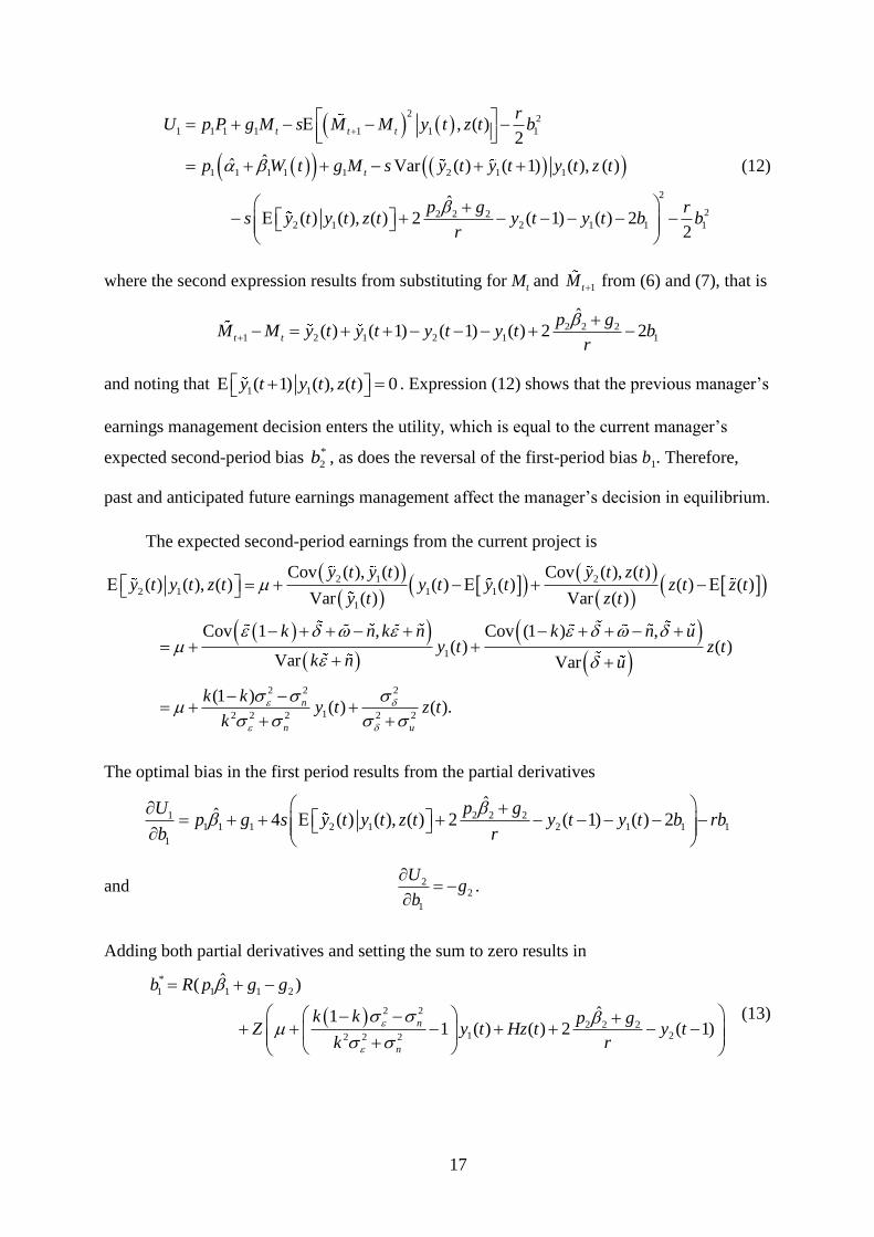
and noting that 1 1E ( 1) ( ), ( ) 0y t y t z t . Expression (12) shows that the previous manager’s
earnings management decision enters the utility, which is equal to the current manager’s
expected second-period bias *
2b , as does the reversal of the first-period bias b1. Therefore,
past and anticipated future earnings management affect the manager’s decision in equilibrium.
The expected second-period earnings from the current project is
2 1 2
2 1 1 1
1
1
2 2
2 2 2
Cov ( ), ( ) Cov ( ), ( )( ) ( ), ( ) ( ) ( ) ( ) ( )
Var ( ) Var ( )
Cov 1 , Cov (1 ) ,( ) ( )
Var Var
(1 ) n
n
y t y t y t z ty t y t z t y t y t z t z t
y t z t
k n k n k n uy t z t
k n u
k ky
k
2
1 2 2( ) ( ).
u
t z t
The optimal bias in the first period results from the partial derivatives
1 2 2 21 1 1 2 1 2 1 1 1
1
ˆˆ 4 ( ) ( ), ( ) 2 ( 1) ( ) 2
U p gp g s y t y t z t y t y t b rb
b r
and 22
1
Ug
b
.
Adding both partial derivatives and setting the sum to zero results in
*
1 1 1 1 2
2 2
2 2 21 22 2 2
ˆ( )
ˆ11 ( ) ( ) 2 ( 1)
n
n
b R p g g
k k p gZ y t Hz t y t
k r
(13)

18
where 1
8R
s r
> 0,
4
8
sZ
s r
> 0, and
2
2 2
u
H
> 0. Further, let
2
2 2 2
n
kQ Z rR
k
> 0. Investors can only observe the total working accruals, which are
*
1 1 1 1( ) ( ) ( )W y t b A Qy t ZHz t (14)
with 2 2 21 1 1 2 2
Known or inferred by market
ˆˆ( ) 2 ( 1).
p gA R p g g Z Z Zy t
r
Investors conjecture that the manager’s earnings report is linear in her private
information y1(t) and z(t). Inspecting expression (14) confirms this conjecture. It also reveals
that W1 negatively (and linearly) depends on y2(t–1), the second-period unmanaged earnings
of the project, which enters the equilibrium bias through the smoothing incentive. Thus, the
bias exhibits not only forward smoothing, but also backward smoothing. y2(t–1) is not directly
observable but can be inferred from other information available at t: The bias *
2b̂ is a constant
(and included in the second term in (14)), and since investors can infer the previous reported
earnings m1(t–1) and, hence, y1(t–1) from the last period, the clean surplus property implies
y2(t–1) = x(t–1) – y1(t–1) where x(t1) are the cash assets in the recent period’s balance sheet.
Thus, even though accounting information about the project t–1 that ends in t is not
informative for valuing the firm, it is nevertheless important for interpreting the current
reported earnings Mt because it is necessary to enable inference of the bias *
1b the manager
adds to the earnings number of the new project t.
The market infers the working capital accruals W1(t) = y1(t) + *
1 1ˆ ( ), ( )b y t z t and uses
them to elicit information about two pieces of information y1(t) and z(t) that the manager
privately knows. Investors revise their expectation of the future cash flow ( )x t of the recent
project as follows:
1
1 1 1
1
Cov ( ), ( )( ) ( ) ( ) [ ( )]
Var ( )t
x t W tx t W t W t W t
W t
2 2
1 12 2 2 2 2 2( ) .
( )n
Qk ZHW t W t
Q k Z H

19
Examination of this expression confirms that the market price effect is a linear function
of W1(t) with
2 2
1 2 2 2 2 2 2
n
Qk ZH
Q k Z H
. (15)
The other terms from the above revised expectation are constant and known or inferred
by investors. In particular, investors are able to directly back out the bias from the price and
earnings incentives.
In the second period, investors use W2(t+1) to revise their beliefs in a similar way. Since
the manager’s bias is a constant, 2 2 22
p gb
r
, the revised expectation is:
2
1 2 2 2
2
2
12 2 2
Cov ( 1), ( 1)( 1) ( 1) ( 1) ( 1)
Var ( 1)
( 1).
t
n
x t W tx t W t W t W t
W t
ky t
k
(16)
Let
2
2 2 2 2.
n
k
k
(17)
Proposition 1 summarizes the analysis and formally states the equilibrium.
Proposition 1: There exists a unique linear equilibrium in which * *ˆj jb b and ˆ
j j , j = 1, 2.
The equilibrium strategies are stated in equations (13), (11), (15), and (17).
Since our main interest is on earnings quality, we only briefly highlight some
characteristics of the earnings management biases *
jb and the market reaction j. Earnings
management in the first period is different to that in the second period. In the second period,
which is the last period in which the manager is active, she is only interested in maximizing
her short-term utility regardless of what happened earlier. This horizon effect makes it easy
for investors to look through the earnings management.
The first-period earnings management strategy is more complex. It includes incentives
that are also effective in the second period, but they also exhibit a desire of the manager to
smooth earnings over periods. Indeed, smoothing is beneficial in this setting because it
induces the manager to use the private information. This smoothing desire leads to forward

20
smoothing, in which the manager considers the effect of a bias in the first period on second-
period earnings. It also leads to backward smoothing because the manager considers the
“inherited” earnings of the project that had been invested by her predecessor. Even though
these earnings cannot be manipulated any more, they affect the level of first-period earnings,
but not of second-period earnings. Therefore, the manager wants to smooth them over the two
periods. In a (unmodeled) longer-term tenure of a manager these interdependencies of past
reported and future anticipated earnings management continue to exist and make the bias even
more complex due to forward smoothing.
The second-period bias *
2b exhibits intuitive comparative statics: It increases in the
weight p2 the manager assigns to the market price reaction and the weight g2 on reported
earnings, and decreases in the cost r of earnings management. A higher market reaction 2 has
more effect on the bias, and since 2 depends on k, 2
, and 2
n , these parameters indirectly
affect the bias.
The first-period bias *
1b comprises the effects of more variables. A higher weight p1
increases the bias, as does a higher weight g1; since the bias reverses in the subsequent period,
the weight g2 enters negatively, however, the anticipated bias *
2b affects the first-period bias
as well, hence, it increases in g2. The net effect depends on the weight s. Then, as mentioned
above, high earnings from the previous year’s project enter negatively to smooth them over
two periods, and both y1(t) and z(t) enter positively. As apparent from (14), the earnings report
is adjusted such that a portion Z = 4s/(8s + r) of the “shocks” y1(t) and z(t) (appropriately
adjusted for their information content) is allocated to the first period, whereas the portion (1 –
Z) is shifted to the second period. If biasing were costless (r = 0), then Z = 1/2 and the shocks
were equally distributed across the two periods and, thus, perfectly smoothed. Z decreases for
higher r.
The coefficients 1 and 2 reflect the sensitivity of investors’ beliefs with respect to the
earnings component that they use to update their expectations. They are given by
2 2
1 2 2 2 2 2 2
n
Qk ZH
Q k Z H
and
2
2 2 2 2.
n
k
k

21
These coefficients are designed to elicit the actual information content of earnings on the cash
flow components and , that are embedded in the accounting signal and the bias. Notice
that 1 and 2 are strictly greater than zero (for parameters bounded away from extreme
values), but can be greater than 1, for example, if k is small. The reason is that k scales the
information contained in y1(t) and, in equilibrium, the market reaction reverses the scaling
effect. More properties of the coefficients 1 and 2 are discussed below.
4. Earnings quality
4.1. Definition of earnings quality
In this section, we study how the design of the accounting system affects earnings
quality. As already mentioned in the Introduction, earnings quality is a notion that captures a
diverse spectrum of attributes of financial reporting and needs specification. We adopt an
information content perspective of financial reports: Reported earnings are of higher quality
the more information they contain with respect to future cash flows.17 This definition is based
on the value of information rather than statistical properties and other concepts.
For normal distributions, the information content of a signal is independent of the
realization of the signals and can be measured by comparing the ex post variance with the
prior variance of the future cash flows.
Definition: Earnings quality EQ is the reduction of the market’s uncertainty about the future
cash flows due to the reported earnings reported in a period t, formally:
Var VarEQ x x M (18)
or equivalently, since the W carries the contemporaneous information in our setting,
2
Cov ,.
Var
x WEQ
W (19)
17 This definition is similar to that, e.g., in Francis, Olsson, and Schipper (2006).
22
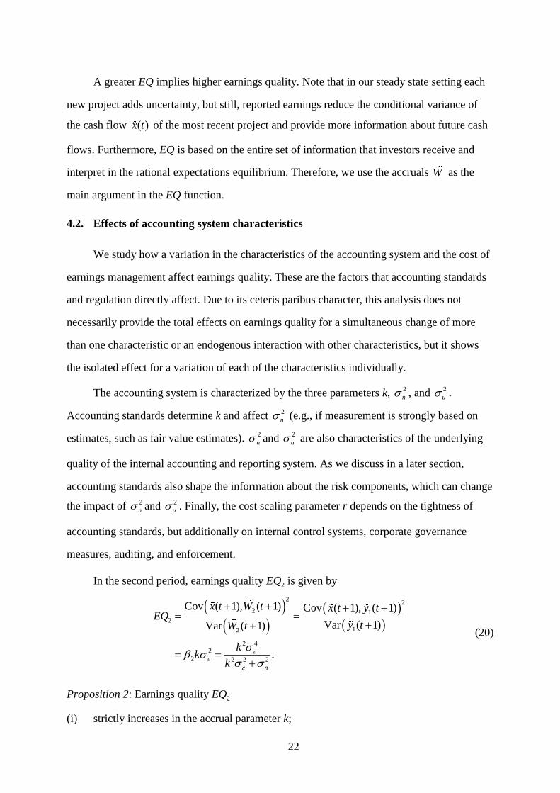
A greater EQ implies higher earnings quality. Note that in our steady state setting each
new project adds uncertainty, but still, reported earnings reduce the conditional variance of
the cash flow ( )x t of the most recent project and provide more information about future cash
flows. Furthermore, EQ is based on the entire set of information that investors receive and
interpret in the rational expectations equilibrium. Therefore, we use the accruals W as the
main argument in the EQ function.
4.2. Effects of accounting system characteristics
We study how a variation in the characteristics of the accounting system and the cost of
earnings management affect earnings quality. These are the factors that accounting standards
and regulation directly affect. Due to its ceteris paribus character, this analysis does not
necessarily provide the total effects on earnings quality for a simultaneous change of more
than one characteristic or an endogenous interaction with other characteristics, but it shows
the isolated effect for a variation of each of the characteristics individually.
The accounting system is characterized by the three parameters k, 2
n , and 2
u .
Accounting standards determine k and affect 2
n (e.g., if measurement is strongly based on
estimates, such as fair value estimates). 2
n and 2
u are also characteristics of the underlying
quality of the internal accounting and reporting system. As we discuss in a later section,
accounting standards also shape the information about the risk components, which can change
the impact of 2
n and 2
u . Finally, the cost scaling parameter r depends on the tightness of
accounting standards, but additionally on internal control systems, corporate governance
measures, auditing, and enforcement.
In the second period, earnings quality EQ2 is given by
22
2 1
2
12
2 42
2 2 2 2
Cov ( 1), ( 1) Cov ( 1), ( 1)
Var ( 1)Var ( 1)
.n
x t W t x t y tEQ
y tW t
kk
k
(20)
Proposition 2: Earnings quality EQ2
(i) strictly increases in the accrual parameter k;

23
(ii) strictly increases in accounting precision ( 21/ n );
(iii) is independent of the precision of non-financial information ( 21/ u );
(iv) is independent of the cost r of earnings management.
The proof follows immediately from the inspection of (20). In particular, EQ2 increases
in the accrual parameter k because a higher k makes contemporaneous earnings
unambiguously more informative about future cash flows. Perhaps less intuitive is the fact
that earnings quality is independent of the precision of non-financial information; the reason
is that in the second period, the manager does not care about injecting her private non-
financial information z(t+1) as she is not interested in future reported earnings and their
interdependence with contemporaneous earnings. EQ2 is unaffected by a variation of the cost
of earnings management. While the amount of bias *
2b clearly depends on the cost of earnings
management r, the market is able to back it out and adjusts the price reaction, so earnings
quality does not change for a change in r.
Earnings quality in the second period is a limiting result as the manager is short-term
interested and does not care about future earnings any more. Earnings quality in the first
period is more descriptive of a typical situation of an ongoing firm. EQ1 is
2 2
2 2
1 2 2
1 12 2 2 2 2 2
1
Cov ( ), ( ).
Var ( ) n
x t W t Qk ZHEQ Qk ZH
Q k Z HW t
(21)
The effects of a variation of the accounting system on EQ1 are more complex because
most of the parameters have an effect on the covariance and the variance terms in (21). To see
what determines the difference between EQ1 and EQ2 it is instructive to briefly consider two
special cases. The first case is when s = 0, i.e., the manager has no incentives to smooth
reported earnings. Then, Z = 0 and Q = 1, and
2 4
1 22 2 2( 0) .
n
kEQ s EQ
k
Without smoothing incentives, the manager does not care about the stochastic time structure
of earnings. Thus, the optimal bias is constant and completely determined by the incentive

24
weights on price and earnings, which is similar to the situation in the second period. Hence,
the market reaction is similar, too.
The second special case is when the manager has no non-financial information, i.e., z(t)
is uninformative, which is equivalent to setting 2
u . Then H = 0 and, again,
2 42
1 22 2 2( ) .u
n
kEQ EQ
k
The reason is that the equilibrium bias *
1b does not contain information on and reduces to a
linear function of y1(t). If s > 0, the manager smoothes earnings which leads to 1Q , but this
does not cause any loss of information for investors since they know Q. Thus, using (14) they
can invert each reported value of the working capital accruals W1(t) to arrive at the actual
value of y1(t). It follows that the information content solely depends on factors driving y1(t),
which mirrors the result for the second period.
Lemma 1: A smoothing incentive (s > 0) and private non-financial information of the manager
outside the accounting signal (2
u ) are necessary and sufficient conditions for reported
earnings to carry incremental information over the accounting signal.
The sufficiency result can be directly seen from the expression of the equilibrium bias
*
1b , which comprises the term ZHz(t). Of course, smoothing requires that the manager’s
decision horizon extends over more than one period. Therefore, in the last period there is no
effect of z(t+1) on reported earnings.
Lemma 1 highlights the importance of a smoothing incentive and earnings management
for conveying additional information through the earnings report to the market. The reason is
that smoothing provides a link between the two periods that the manager is motivated to
embed in the bias part of her private information.
Proposition 3 reports the results for the general case, in which the parameters are not in
the extremes.
Proposition 3: Earnings quality EQ1
(i) strictly increases in the accrual parameter k for low k; for high k it can decrease

25
(a necessary condition is
22
2
4 n nsk
r
);
(ii) strictly increases in accounting precision 2(1/ )n ;
(iii) strictly increases in the precision of non-financial information ( 21/ u );
(iv) strictly decreases in the cost r of earnings management.
The proof is in the appendix. It consists of signing the partial derivatives of EQ1 with
respect to each of the parameters. The proof is straightforward, although some of the steps are
lengthy. In the following, we explain the results and provide the intuition for them.
Accrual parameter
The effect of a variation of k is complicated because k affects both components of
1( ),W t y1(t) and *
1b . An increase in k places a greater portion of into contemporaneous
earnings y1(t), hence, earnings become more informative about future cash flows, which
would increase earnings quality if everything else was held constant. In particular, k = 1
should maximize earnings quality. However, as stated in the proposition, the intuition holds
for low k, whereas there are settings with high k in which an increase in k actually reduces
earnings quality. The reason for this effect is that the parameter k not only changes the
information content of y1(t), but also affects the weights with which financial and non-
financial information are processed in the market. A more informative y1(t) can reduce the
equilibrium weight of z(t), thus driving out the non-financial information for pricing the firm.
Note that k is a smoothing mechanism embedded in the accounting system, in addition to that
in the bias *
1 .b Embedded smoothing is low for extreme values of k; and would be fully
smoothed across the two periods if k = 1/2.
To gain further insight into the result, consider a special case with a fully precise
accounting system (2
n = 0) and no non-financial information by the manager (2
u ).
Then, as noted above, EQ1 = EQ2, and due to 2
n = 0, EQ1 = 2
, which is constant and
independent of k. Formally, the squared covariance in the numerator of EQ1 and the earnings
variance in the denominator change exactly by the same factor, 2k, for a change of k.
Intuitively, k serves only as a scaling factor of the risk component without affecting its

26
information content. Indeed, 2 =1/k in this special case, so the market reaction simply adjusts
for the level of k. *
1b still smoothes earnings across the two periods, but its size depends on
1/k as well.
Reintroducing non-financial information 2( )u destroys this one-to-one relationship
because an increase in k increases the (squared) covariance between earnings and the future
cash flow and the variance of earnings at different rates. This is because k now affects the
weights with which the two informative signals y1(t) and z(t) enter the reported earnings. It
can be shown that the variance increase dominates the covariance increase, so actually an
increase in k reduces earnings quality EQ1 as long as the accounting system is precise.
Intuitively, an increase in k scales without harming the information content of the signal
y1(t), but at the same time the larger variance of earnings dilutes the information that earnings
carry about z(t).
Coming back to the general case, if the accounting system is noisy (2
n > 0) then an
increase in k increases the weight of in y1(t), which individually increases the information
content of earnings and, hence, positively affects earnings quality. Starting at k = 0, an
increase in k always increases EQ1, but for high k the variance-increasing effect can dominate.
This result exhibits a subtle interaction between the accounting system (as captured by
k), earnings management, and earnings quality. Bringing into the accounting system more
information about future cash flows can reduce earnings quality, particularly if the accounting
system is relatively imprecise. The proposition states a necessary condition for EQ1 to
decrease in k, which is
22
2
4 n nsk
r
, hence, the lower the right-hand side of this
expression is the more likely is a decrease. Notice that the right-hand side is zero for 2 0n
and achieves a unique maximum for
2
2 2ˆ 4n
s
r
.
Differentiating the right-hand side of this bound with respect to yields

27
2
2
2
4
42 .
n n
n n
s
r s
r
The derivative is positive if 2
n
s
r , which is equivalent to 2 2ˆ
n n , and vice versa.
Taken together, this leads to the following prediction:
Corollary 1: A decrease in earnings quality EQ1 in k is more likely
(i) the lower is the accounting precision 2(1/ )n if 2 2ˆn n ;
(ii) the lower is the operating risk 2
if 2 2ˆn n ;
(iii) the lower is the smoothing incentive s;
(iv) the higher is the cost r of earnings management.
Accounting precision
A decrease of the accounting precision (a higher noise variance 2
n ) lowers the
covariance of earnings with future cash flows and affects the variance of earnings in two
ways: First, the variance increases due to the direct impact of a larger accounting noise.
Second, the variance decreases due to the negative impact of a greater 2
n on the weight Q
with which the signal y1(t) enters reported earnings. While the first variance effect works in
the same direction as the covariance effect, the second is in the opposite direction. The
proposition states that the latter effect is dominated, so that higher accounting noise and lower
accounting precision, respectively, unambiguously reduces earnings quality. This effect is
similar to the effect on EQ2, although it is not as straightforward.
Notice that an individual variation of either k or 2
n affects the precision of the
accounting signal similarly: Higher k is similar to an increase in the precision (given some
2 )n , and lower 2
n is similar to an increase in the precision (given some k). This result
reinforces the earlier discussion that the surprising effect on earnings quality for a variation of
k is attributable to the built-in smoothing effect of k, which affects the weights of the two
informative signals.

28
Precision of non-financial information
The precision of the manager’s non-financial information is determined by the variance
of the noise 2
u in the signal z(t) the manager obtains early about the cash flow component .
Given a certain level of operating risk 2
, higher noise 2
u unambiguously reduces the
information contained in z(t), which is brought into reported earnings through the manager’s
bias. Therefore, earnings quality strictly decreases in 2
u and increases in the precision of the
manager’s information, respectively. Note that this effect does not occur for second-period
earnings quality (in Proposition 2) because the manager does not care about that information
in the last period of tenure.
One might argue that more non-financial information increases the information
asymmetry between the manager and investors and motivates the manager to exploit this
comparative advantage by more offensive earnings management, which should decrease
earnings quality. Indeed, the bias *
1b includes a greater portion of the signal z(t) and reacts
more strongly to it, but investors rationally anticipate this effect and adjust the market price
reaction accordingly. In total, earnings become more informative and earnings quality
increases the more precise is the non-financial information of the manager.
Cost of earnings management
Without smoothing, the cost of earnings management, captured by the scaling parameter
r, has no effect on earnings quality. This can be seen from EQ2. Therefore, if a change of r has
an effect on earnings quality it must be through the smoothing incentive. As stated in the
proposition, an increase in r reduces earnings quality EQ1 because it reduces the level of the
bias and, hence, the information content of the bias reduces relative to that in y1(t).18
Contemporaneous earnings reveal less information about z(t), and this reduces earnings
quality. As stated in Proposition 2, once z(t) becomes uninformative, r dampens the level of
earnings management, but this has no effect on earnings quality any more.
18 This effect is economically similar, but converse, to an increase in the smoothing parameter s.

29
4.3. Effects of operating risk
To examine whether and how characteristics of the firm’s operations affect earnings
quality, we consider variations of the variances 2
, 2
, and 2
of the three cash flow
components , , and on EQ1 and EQ2. The variances depend on the business model, the
short-term or long-term volatility of the production process, and the firm’s environment.
Since we orthogonalize these components, the variation of one variance additively changes
total operating risk.
This analysis provides insights how – these operating characteristics influence earnings
quality, keeping the accounting system constant. The results are useful in at least two respects.
First, they help understand the effect of information while keeping the total cash flow
variance 2 2 2
, constant. For example, the accounting system may be designed to
provide information about a greater portion of the future cash flows (which can be modeled
by 2
and 2
) or the manager may be able to receive more information about the
cash flow, which is not recognized by the accounting system (2
and 2
). Second,
empirical studies often control for innate factors that capture the business model and the
characteristics of the firms’ operations (see, e.g., Francis, Olsson, and Schipper 2006) when
they attempt to isolate the effects of a change in the accounting characteristics. Therefore, it is
useful to know how these effects influence earnings quality measures.
Proposition 4: Operating risk affects earnings quality as follows:
(i) EQ1 strictly increases in 2
for high 2
(a sufficient condition for all 2
is
2
2 2 2 2 2 02 2
n n u
r r
s s ); it can strictly decrease for low
2
;
EQ2 strictly increases in 2
;
(ii) EQ1 strictly increases in 2
; EQ2 is independent of 2
;
(iii) EQ1 and EQ2 are independent of 2
.
The proof is in the appendix.
The effects on earnings quality differ significantly for the three risk components. The
reason does not rest in the operations themselves, but in the different information that is

30
available about the cash flow components: The accounting system reports accounting earnings
that are informative about ; the manager obtains private information about that is not
included in the accounting earnings; and there is no additional information available on .
The key accounting variable is W1(t), which carries information about and, indirectly, about
through the equilibrium bias.
Generally, a higher variance of cash flows makes accounting information about that
component more useful, and the impact on earnings quality should be higher. However, this
intuition is incomplete. First, note that the residual volatility of the future cash flow, measured
by the variance 2
, does not affect earnings quality. The reason simply is that reported
earnings contain no information about , so there is no decrease in the variance of future
cash flows. This independence result makes it simple to generate predictions about keeping
the total variance of the cash flows constant, but simultaneously changing either 2
or 2
and 2
by the same amount in the reverse direction. All results we state in the proposition (i)
and (ii) are preserved.
The manager learns about the second cash flow component from privately observing
z(t) = u . In the second period of tenure, the manager does not base the bias on z(t+1), so
W2 does not carry information about of the concurrent project; therefore, EQ2 is unaffected.
This is different from the first period, where z(t) is embedded in *
1b . The information content
of z(t) depends on the relative risks of the two components. Fixing some 2
u , an increase in
the volatility of the cash flow component 2
increases the information content of z(t), which
induces an increase in earnings quality.
Finally, consider a variation of the risk of the cash flow component . A logic similar
to the one above applies for EQ2, so EQ2 increases in 2
. However, the effects of varying 2
on EQ1 are more complicated because 2
affects the information content ofy1(t) and of the
bias *
1b . The proposition states that EQ1 strictly increases in 2
for high 2
, but can strictly
decrease in 2
for low 2
. The proof provides a sufficient condition for a strict increase over
all 2
, which is
2
2 2 2 2 2 0.2 2
n n u
r r
s s

31
This condition holds, for example, if 2
is low, if 2
n is large, if r is high, or if s is low. The
converse of this condition is a necessary condition for a decrease of EQ1 in 2
. EQ1 can only
decrease for low 2
and will always increase for sufficiently high 2
. Intuitively, an increase
in 2
can significantly increase the variance of reported earnings, thus, lowering the
precision of these earnings and diluting the information that can be inferred about the signals
y1(t) and z(t). This negative effect can overcompensate the benefit of conveying more
information about . This result mirrors that for a variation of k.
5. Value relevance and earnings quality
The analysis has established how a variation of individual characteristics of the
accounting system affects earnings quality, defined as information content of reported
earnings. Since earnings quality is not directly observable, the empirical accounting literature
uses several measures as proxies for earnings quality (see, e.g., Francis, Olsson, and Schipper
2006 and Dechow, Ge, and Schrand 2010). In this section, we study how one common
measure, value relevance, is related to information content. We select value relevance as it is
closely related to our rational expectations capital market model.19 Value relevance is used in
many studies, but is a controversial measure for earnings quality (see, e.g., Holthausen and
Watts 2001).
Value relevance captures the notion that earnings are of high quality if they are capable
to explain the firm’s market price and/or market returns. Most common are two measures: the
earnings response coefficient, which is the coefficient of the earnings variable in a regression
of the market price and/or return on earnings; and the R2 from the price-earnings regression.
Our analysis provides theoretical insights into the question how well these value relevance
measures perform as proxies for earnings quality. We also address the question under what
circumstances one of the two measures is a preferable proxy.
An empirical study uses reported earnings at face value and relates them to market
prices (or price changes), whereas investors perform several adjustments when they interpret
19 Accounting-based measures are examined in Ewert and Wagenhofer (2013).

32
reported earnings and other information available (book values and prior period earnings) in
order to elicit the information about the interesting signals y and z . While one may argue if
this is a fair comparison, this in fact is what empirical studies usually do.20 Hence, we do not
expect that these proxies perfectly trace earnings quality.
We focus on the first period of a manager’s tenure as it is more representative of firms
in a cross-sectional analysis. While the second period has a strong effect on earnings quality
(as stated in proposition 2 in comparison to proposition 3), the horizon effect is weaker in this
analysis as total reported earnings always include two active projects. Formally, in the first
period investors base their pricing decisions on the working capital accruals W1(t) rather than
on the reported earnings Mt, where
1
*2 2 22 1 1
( )
1 .t
W t
p gM y t I y t b
r
It is easy to see that tM depends on the period t earnings of the projects initiated in t and t–1.
Therefore, the statistical relationships of prices with tM are different from those with 1( )W t ,
which implies that the behavior of value relevance measures also differs from that of actual
earnings quality. To eliminate a “mechanistic” co-variation of earnings and prices that
depends on the cash position from the project that ends at the end of the period, we use ex
dividend prices in the subsequent analysis.21
5.1. Earnings response coefficient
The earnings response coefficient (ERC) is the market price reaction to (unadjusted)
reported earnings. In our model, it is the direct equivalent to the capital market reaction on
reported earnings and is defined as
20 While more variables are often included in a price-earnings regression, we believe that there will still be
differences due to the structural assumptions underlying linear regressions.
21 This is consistent with empirical value relevance studies based on level regressions, which typically use prices
lagging a few months after the fiscal year end. Using cum dividend prices would add terms to the covariance and
variance terms in the analysis that do not vary with the information content of reported earnings, but may affect
the results.

33
1
Cov ,
Var
t t
t
P MERC
M .
This formulation captures a cross-sectional analysis of a sample of firms drawn from our
stochastic setting. To calculate this term, note that the equilibrium price depends only on
1( )y t and ( )z t because investors infer and correct for the earnings of the “inherited” project,
2 ( 1)y t . However, the accruals 1W t include 2( 1)Zy t through the bias (see equation
(14)), which is eliminated by using the following price equation,
1 1 1 2 1tP W t Zy t .
Note that this modification applies for tP but not for tM . The earnings response coefficient
then is
1 1 2
1
1 2 1 2
1
1 1
1
11
1
Cov ( ) ( 1) ,Cov ,
Var Var
Cov ( ) ( 1), ( ) ( 1)
Var
Cov ( ) ( ) , ( ) ( )
Var
Cov ( ), ( )Var ( ) ( )
Var Var
tt t
t t
t
t
t t
W t Zy t MP MERC
M M
W t Zy t W t y t
M
Qy t ZHz t Qy t ZHz t
M
x t W tQy t ZHz t
M M
2 2
2 22 2 2 2 2 2 2 2 2 2.
1 1n n
Qk ZH
Q k Z H Z k
(22)
It is apparent that ERC1 and 1 are closely related, and they are scaled by a factor that
depends on the variances of the informative part of earnings and the reported earnings.
Proposition 5: The earnings response coefficient ERC1
(i) strictly increases in the accrual parameter k for low k; for high k it can decrease
(a necessary condition is 2 2 2
nk );
(ii) strictly increases in accounting precision 2(1/ )n ;
(iii) strictly increases in the precision of non-financial information (21/ u );

34
(iv) strictly decreases in the cost r of earnings management if r is sufficiently large;
it can increase for low r.
The proof is in the appendix.
The result for a variation of the accrual parameter k is structurally similar to that of
earnings quality EQ1. Increasing k increases ERC1 if k is low (sufficient condition). If k is
large there are parameter constellations in which ERC1 decreases. The underlying reason is
similar to that for EQ1, but the condition for which the effect reverses differs. In Proposition
3, the necessary condition is
22
2
4 n nsk
r
whereas here it is 2 2 2
nk , which does not depend on s and r. Therefore, using ERC1 as a
measure for a change in earnings quality can lead to wrong conclusions; the error can be in
either direction. For example, if 2
n is equal to2
, then ERC1 always increases for any k,
whereas earnings quality can decrease if k > 4s/r, which holds for high r although this is
commonly considered an indicator of a high-quality reporting system.
Increasing the precision of the accounting signal (decreasing the variance 2
n ) or
increasing the precision of the non-financial information (decreasing the variance 2
u )
unambiguously increases the ERC1. These results are similar to earnings quality EQ1,
therefore, the earnings response coefficient is a useful measure of earnings quality if there is a
variation in the precision of the internal management accounting system.
An increase in the cost r of earnings management can lead to different effects on ERC1
and EQ1. While EQ1 unambiguously decreases in r, this is not necessarily true for ERC1 as it
can increase if r is small until it attains a maximum and decreases afterwards. This behavior is
inconsistent with that of EQ1 for small r, e.g., for imprecise accounting standards or low
auditing and enforcement standards.
To gain more intuition, consider the boundary case with r = 0, so that biasing is costless
and unlimited smoothing occurs. For k > 0.5, the built-in smoothing of the accounting system
with respect to the risk component is “too large” from the manager’s point of view, hence,

35
a negative bias is preferable. Costless smoothing implies that a relatively large portion of the
variability of is smoothed away, leading to a lower covariance between the reported portion
of and future cash flows than would occur if k was reported without bias. In addition, if
there is large accounting noise, the desire to negatively bias the signal y1(t) is even stronger,
which further reduces the covariance. An increase of r (starting from r = 0) makes smoothing
more expensive and has two effects on the covariance: First, the weight with which z(t) enters
reported earnings diminishes, thus lowering the covariance term in the numerator of ERC1.
Second, the manager reduces the smoothing of y1(t) which increases the covariance term
under the assumed setting of parameters. If the variance 2
of the risk component and/or
the precision of the manager’s signal z(t) are low, the first effect is relatively minor, resulting
in a net increase of the covariance term.
Of course, the impact on ERC1 depends on the ratio of the covariance and the variance
of total reported earnings which increases by increasing r, but the effect on the numerator may
dominate, so that ERC1 can increase in r for small r. As shown in the proof, this does not hold
for all r. If the risk 2
is large, then the negative impact of an increase of r on the weight of
z(t) in the earnings report dominates, implying a lower covariance for larger r. Then ERC1
decreases for increasing r.
The behavior of the earnings response coefficient in the second period, ERC2, is similar
to that of ERC1, hence, we do not report it here.
In summary, the ERC is generally a good proxy for earnings quality, particularly if the
variations relate to changes in the precision of the accounting system or non-financial
information. However, there are settings in which ERC leads to results opposite to those for
earnings quality for variations in the accrual parameter and the cost of earnings management.
5.2. Correlation coefficient
The R2 of a price-earnings regression translates into the correlation coefficient (CORR)
in our model. It is defined as
1
Cov( , )
Std( )Std( )
t t
t t
P MCORR
P M ,

36
which is equal to (shown in the appendix)
2 2 2 2 2 2
1 2 22 2 2 2 2 2 2 2 2 2.
1 1
n
n n
Q k Z HCORR
Q k Z H Z k
(23)
This measure differs from the ERC1 only in that the denominator includes Std( )tP
instead of Std( )tM . Despite this close relationship, the effects of a variation of the accounting
characteristics are significantly different.
Proposition 6: The correlation CORR1
(i) strictly increases in the accrual parameter k;
(ii) can strictly increase or decrease in accounting precision 2(1/ )n depending on
parameters;
in particular, if k < 4s/r, then CORR1 strictly decreases in 2
n for small 2
n and
can increase for large 2
n ;
(iii) strictly increases in the precision of non-financial information (21/ u );
(iv) can strictly decrease or increase in the cost r of earnings management.
The proof is in the appendix.
The correlation strictly increases in the accrual parameter k, which is in contrast to the
behavior of EQ1. Recall that EQ1 can decrease for high k under certain conditions.
A decrease in accounting precision (a higher variance 2
n ) either decreases or increases
the correlation. This result is also in contrast to EQ1, which always decreases in 2
n . To see
why CORR1 can increase in 2
n assume k > 4s/r. In the appendix, we show that if the residual
risk 2
is large enough, then 1CORR increases in 2
n for all levels of 2
n . Intuitively, if k >
4s/r then the impact of the incentive to smooth earnings is small, so that a larger accounting
noise increases the variance of both the informative part of earnings 1( )W t (the working
capital accruals) and reported total earnings tM . While the absolute increase of the variance
of total earnings (the denominator of CORR1) is larger than that of the informative part of
earnings (affecting the numerator), the relative change is stronger for the numerator if there is
large risk in total earnings (e.g., for a high 2
), yielding an increase in the correlation

37
coefficient. Conversely, k < 4s/r implies that the smoothing incentive is relatively strong,
inducing the manager to dampen the impact of a larger accounting noise by smoothing. Then
the variance of the informative part of earnings decreases by introducing accounting noise.
This leads to a reduction of CORR1 for small accounting noise, but this behavior may change
for larger 2
n .
CORR1 strictly increases in the precision of non-financial information (decreases in the
variance 2
u ), which is consistent with the behavior of EQ1.
Finally, CORR1 can strictly decrease or increase in a variation of the cost r of earnings
management, depending on the parameters. The reason lies in the impact that the cost of
smoothing has on the variances of the informative part of earnings 1( )W t and reported total
earnings tM . To illustrate the possible effects, consider the boundary case r = 0 in which the
manager’s bias is determined only by smoothing considerations, so the manager chooses the
maximum amount of smoothing (i.e., Z = 0.5). Here the manager incorporates z(t) with the
maximum weight into reported earnings, which has a strong impact on the variance of 1( )W t .
An increase in r now dampens the weight of z(t) and leads to a reduction of the earnings
variance. At the same time, the higher cost also dampens the incentive to smooth the other
risks, and depending on the relative size of these risks (accounting noise and operating risks),
the ratio of the two variances in CORR1 can increase or decrease. Note that EQ1 always
decreases in r, thus the behavior of the correlation coefficient differs from that of earnings
quality.
A similar analysis of the second-period correlation CORR2 yields similar results.
Taken together, comparing the behavior of CORR1 and ERC1 with that of earnings
quality EQ1 shows that neither of the two proxies perfectly traces EQ1 in a simple price-
earnings regression. ERC1 is generally a more reliable proxy than CORR1 because its behavior
is better aligned with that of EQ1 in more situations. We should note, though, that the
correlation is often used in regressions with more than one independent variable, such as
changes in earnings or net assets. In that case, the ERC cannot capture the total effect and may

38
perform worse. Therefore, an empirical design choice faces a trade-off between these two
effects.
5.3. Forward changes of parameters
The analysis so far has implicitly assumed that a change in one parameter is effective
over the entire time the firm exists. For example, changing k essentially compares two
different regimes, one in which k is unaffected and the other in which k is different. Such an
analysis is helpful to assess the earnings quality of different accounting systems. In an
empirical study, it is particularly applicable to international, cross-country studies.
An alternative research question is, what are the immediate effects of a change of a
parameter effective at a certain date? In this case, the equilibrium strategies before that date
are governed by the original parameter value, and afterwards they are based on the changed
parameter value. Indeed, many empirical studies examine the effect of a change of the
accounting regime in a jurisdiction. Formally, the effect of a change does not alter the past,
but only the future, assuming that managers do not anticipate the change.
Note that the equilibrium effects of a variation of the parameters on earnings quality EQ
are unaffected by this forward change because investors base their price reaction on the
inferred working capital accruals ( )jW t , where
W1(t) = y1(t) + b1 and W2(t) = y1(t) + b2.
Therefore, ( )jW t captures only forward-looking information. Past effects are included in the
fixed term t of the market pricing equation and do not affect earnings quality.
In contrast, value relevance is based on reported total earnings tM , which aggregate
earnings from two overlapping projects in the following way:
1
* *
2 2 1 1
( )
1 .t
W t
M y t b I y t b
A forward change of a parameter does not affect the distribution of 2 ( 1)y t because it is
governed by the previous parameter value, but it affects only the distribution of those parts of

39
( )jW t that are independent from 2 1y t . Therefore, the effects of a forward change on
ERC1 and CORR1 differ from those presented in Propositions 5 and 6.
For the sake of brevity, we do not repeat the analysis for this situation and just note that
some of the results are unchanged, others show even stronger deviations from those for EQ1,
and still others are mitigated. To illustrate the latter effect, consider the effect of an increase in
accounting risk 2
n on CORR1. If only forward changes are considered, then both the
numerator and the denominator of CORR1 increase by the same amount, implying a strict
increase in CORR1. This eliminates the ambiguous effect recorded in Proposition 6 (ii) and
aligns the behavior of CORR1 with that of EQ1 for a variation of 2
n .
6. Conclusions
This paper shows that some intuitively plausible effects of a change in accounting
standards and the institutional financial reporting setting on earnings quality are not generally
valid. In particular, we identify earnings smoothing incentives by management as crucial that
earnings management incorporates some of the manager’s private information. A main result
of the analysis is that making accounting earnings more informative reduces earnings quality
under certain conditions. Changing the information content also affects the weights with
which financial and non-financial signals enter the bias, hence, a more informative accounting
signal can drive out the non-financial information in reported earnings. Collectively, this
change can generate lower-quality earnings in the capital market. Another main result is that
an increase in the cost of earnings management (e.g., less discretion, higher audit and
enforcement quality) reduces earnings quality. This change diminishes the ability of the bias,
and reported earnings, to convey private information. We derive these effects in a rational
expectations equilibrium that features a steady state firm with investment in every period, an
accounting system, non-financial information, and earnings management.
We also examine how accurately value relevance measures, the earnings response
coefficient and the correlation of a price-earnings regression, trace the changes in the
information content of earnings induced by a variation of the characteristics. They perform
well for a variation of some characteristics, but may lead to wrong conclusions for other

40
characteristics. We also show that the effects differ whether one compares firms following
different accounting standards or one studies a change in accounting standards for the same
firms.
The model features several key ingredients of accounting standards, including the
recognition of accruals and the precision of measurement in an ongoing firm. However, we
use several simplifying assumptions to keep the analysis tractable, which may affect the
generality of our findings. We emphasize three of them. One assumption is that, although we
study a production setting with periodic investment decisions, we do not explicitly model
decisions by management that affect the future cash flows (see Kanodia (2006) for such
models). While the cost of earnings management is a “real” cost, for simplicity we assume
this cost arises as private disutility of the manager and is not mirrored in the firm’s cash
flows. Moreover, if investment affects future expected cash flows, as long as shareholders
obtain sufficient information about this investment, our results would not qualitatively
change. Our analysis is useful for broader models for at least three reasons: (i) It provides
insights if the production effect is not of first-order interest; (ii) it is descriptive of situations
in which the information affects production decisions later, if these decisions are not directly
linked with the utility of the manager; and (iii) it examines a second step, after production
decisions have been taken, perhaps even based on the anticipated reporting strategy.
Our analysis examines ceteris paribus changes of individual characteristics of the
accounting system. For example, we assume the manager’s incentives are exogenously fixed
and are not adjusted to a change in the respective characteristic. In a more general setting,
incentive contracts would determine the weights endogenously. Further, the market discount
factor may depend on the amount of information about the firm. Our analysis states that
earnings smoothing, for whatever reason it obtains, can have unintended consequences in
standard setting, and we believe that this result does not disappear in a more inclusive model.
Finally, we note that earnings management is informationally not harmful in our setting;
investors are able to elicit the essential decision-useful information in equilibrium on average.
It is only the cost of earnings management that makes it undesirable. This is consistent with

41
the view that earnings management signals private information (which drives our results),
while opportunistic elements are correctly recognized by investors in interpreting the earnings
report. Extending the analysis to allow for additional economic forces provide fruitful
opportunities for further research.

42
References
Christensen, P.O., G.A. Feltham, and F. Şabac (2005). A Contracting Perspective on Earnings
Quality. Journal of Accounting and Economics 39: 265-294.
Christensen, J., and H. Frimor (2007). Fair Value, Accounting Aggregation and Multiple
Sources of Information. In: R. Antle, F. Gjesdal, and P.J. Liang. Essays in Accounting
Theory in Honour of Joel S. Demski, New York: Springer: 35-51.
Christensen, P.O., H. Frimor, and F. Şabac (2013). The Stewardship Role of Analyst
Forecasts, and Discretionary Versus Non-discretionary Accruals. European Accounting
Review 22: 257-296.
Cho, K., and D.M. Kreps (1987). Signaling Games and Stable Equilibria. Quarterly Journal
of Economics 102: 179-221.
De Jong, A., G. Mertens, van der Poel, M., and van Dijk, R. (2012). How Does Earnings
Management Influence Investors’ Perceptions of Firm Value? Survey Evidence from
Financial Analysts. Unpublished working paper, Erasmus University.
Dechow, P.M., W. Ge, and C. Schrand (2010). Understanding Earnings Quality: A Review of
the Proxies, Their Determinants and Their Consequences. Journal of Accounting and
Economics 50: 344-401.
Demski, J.S. (1998). Performance Measure Manipulation. Contemporary Accounting
Research 15: 261-285.
Dichev, I., J. Graham, C.R. Harvey, and S. Rajgopal (2013). Earnings Quality: Evidence from
the Field. Journal of Accounting and Economics (forthcoming).
Drymiotes, G., and T. Hemmer (2013). On the Stewardship and Valuation Implications of
Accrual Accounting Systems. Journal of Accounting Research 51: 281-334.
Dye, R.A. (1988). Earnings Management in an Overlapping Generations Model. Journal of
Accounting Research 26: 195-235.
Dye, R.A., and S.S. Sridhar (2004). Reliability-Relevance Trade-offs and the Efficiency of
Aggregation. Journal of Accounting Research 42: 51-88.
Dutta, S. and S. Reichelstein (2005). Stock Price, Earnings, and Book Value in Managerial
Performance Measures. The Accounting Review 80: 1069-1100.
Dutta, S. (2007). Dynamic Performance Measurement. Foundations and Trends in
Accounting 2: 175-240.
Einhorn, E., and A. Ziv (2012). Biased Voluntary Disclosure. Review of Accounting Studies
17: 420-442..
Ewert, R., and A. Wagenhofer (2013). Earnings Quality Metrics and What They Measure.
Working Paper, University of Graz.
Fischer, P.E., and P.C. Stocken (2004). Effect of Investor Speculation on Earnings
Management. Journal of Accounting Research 42: 843-870.
Fischer, P.E., and R.E. Verrecchia (2000). Reporting Bias. The Accounting Review 75: 229-
245.
Francis, J., P. Olsson, and K. Schipper (2006). Earnings Quality. Foundations and Trends in
Accounting 1(4): 259-340 (1-85).

43
Graham, J.R., C.R. Harvey, and S. Rajgopal (2005). The Economic Implications of Corporate
Financial Reporting. Journal of Accounting and Economics 40: 3-73.
Guttman, I., O. Kadan, and E. Kandel (2006). A Rational Expectations Theory of Kinks in
Financial Reporting. The Accounting Review 81: 811-848.
Holthausen, R.W., and R.L. Watts (2001). The Relevance of the Value-relevance Literature
for Financial Accounting Standard Setting. Journal of Accounting and Economics 31: 3-
75.
Huson, M.R., Y. Tian, C.I. Wiedman, and H.A. Wier (2012). Compensation Committees’
Treatment of Earnings Components in CEO’s Terminal Years. The Accounting Review
87: 231-259.
Kanodia, C. (2006). Accounting Disclosure and Real Effects. Foundations and Trends in
Accounting 1(3): 1-95.
Kirschenheiter, M., and N.D. Melumad (2002). Can “Big Bath” and Earnings Smoothing Co-
exist as Equilibrium Reporting Strategies? Journal of Accounting Research 40: 761-
796.
Marinovic, I. (2013). Internal Control System, Earnings Quality, and the Dynamics of
Financial Reporting. Rand Journal of Economics 44: 145-167.
Sankar, M.R., and K.R. Subramanyam (2001). Reporting Discretion and Private Information
Communication through Earnings. Journal of Accounting Research 39: 365-386.
Stocken, P.C., and R. Verrecchia (2004). Financial Reporting System Choice and Disclosure
Management. Review of Accounting Studies 79: 1181-1203.
Trueman, B., and S. Titman (1988). An Explanation for Income Smoothing. Journal of
Accounting Research 26, Supplement: 127-139.
Tucker, J.W., and P.A. Zarowin (2006). Does Income Smoothing Improve Earnings
Informativeness? The Accounting Review 81: 251-270.

44
Appendix
Proof of proposition 3
The partial derivative of EQ1 with respect to any parameter i has the following form:
11 11 1
1 1
1 1
12
1
1
1
( ), ( )Cov ( ), ( )
Cov ( ), ( ) Var ( )Var ( ) Cov ( ), ( )
Cov ( ), ( )Var ( )
Cov ( ), ( )
Cov x t W tEQx t W t
i i i
x t W t W tW t x t W t
i i x t W tW t
x t W t
i
1 11
1 1
1
Cov ( ), ( ) Var ( )2 Var ( ) Cov ( ), ( )
Var ( )
B
x t W t W tW t x t W t
i iW t
(A1)
Since 1 and 1Var ( )W t are positive, the sign of the derivative of EQ1 is the same as the sign
of B as defined in (A1). For the rest of the proof it useful to collect the following derivatives:
2 2 2 2
2 22 2 2 2 2 2
2 22 2 2 2 2 2
4 , 4 , 8 , 8
4 8 4 2 , 4 8 4 2 .n n
rR rRZ ZrR sR rR sR
s r s r
k kQ QrR rR rR sR sR sR
s k r k
(i) Accrual parameter k
The two components of the partial derivative with respect to k are (using Q Q k )
1 2 2
1 2 2 2 2 2
Cov ( ), ( )2 2
Var ( )2 2n
x t W tQ k Q
k
W tQQ k Q k
k
Using these expressions,
2 2 2 2 2 2 2 2
2 2 2 2 2 2 2
2
2 2 .
n
n
B Q k Q Q k Z H
Qk ZH QQ k Q k
Multiplying out, cancelling common terms and rearranging yields B = B1 + B2, where

45
2 2 3
1
2 2 2
2
2
2
n
n
B Q
B ZH Q k Q Z kQ QQ
We note that B1 > 0. To determine the sign of B2 we start with expanding the difference
Z – kQ in B2 which yields:
2 2 2
22 2 2 2 2 21
n n
k kZ kQ Z k Z rR Z Z krR Z k krR
k k
Next we expand ( )Q k Q and compute 2
nQQ :
22 2 2 2
22 22
2 2 2
22
2 2 2 2 2 2 22 2 2
2 2
1
2 1 0
n
n
n
n
kQ k Q Z k Z rR Zk Z rR
k k
Z Z k Z rR Z k k Z rRk
Z k rR
22 2 2 2
22 2 2
2 2 222 2 2
22
2 2 2 2
2 22 2 2 2
2 2 2 2 2 2 2
2 2
2 2 2 2 2
1 1
1 1
1 1 1 1
1 1 2 1 1 2
n
n n
n
kQ Q Q Z Q Z k k k
k
Z rR Z k k k
Z k Z k k rR Z k rR Z k k
Z k k rR Z k k
The difference of these terms is
2 2
2
2 2 2 2
2 2
2 2 2 2 2
2
2 2 2 2 2
22 2
2 2 2 2
2
2 2 2 2 2
2
1 2 1
1 1 2 1 1 2
1 2 1 1 2
1 1
1 1 2 1 1 2
2
nQ k Q Z kQ QQ
Z k Z rR Z k k rR
Z k k rR Z k k
Z k k k rR Z k
Z k k rR Z rR Z k k rR
Z k k rR Z k k
k rR Z
22
2 2 2 2 2
2 2
22 2
2 2
1 1 1
1 1 2
1
k Z k rR Z k k rR
rR Z k k
Z k k rR
Taken together, B becomes:

46
22 2 3 2 2
1 2 2 22 1n
C
B B B Q ZH Z k k rR
If C ≥ 0 then B is positive and EQ1 increases unambiguously in k. Otherwise, B can
always become negative because 2
can be set high enough to result in B < 0. C is negative if
2 2
2 22 2
2 2 22 2 2
22
2
1
4
n
n
n n
kZ k k rR Z k rR
k
sk
r
Thus, there exists a threshold ≥ 0 such that C < 0 iff k > , where
2
2
2
2
40 if 0
4otherwise
n n
n n
s
r
s
r
Notice that even if = 0 and thus C < 0 for all positive k, the derivative of EQ1 with
respect to k is always positive for k = 0 because then 2 = 0, C = 0, Q = rR and therefore
32 20 2 0nB k rR .
Therefore, if the threshold ≥ 1, then EQ1 is strictly increasing in k; if < 1, then EQ1
may reach a maximum with respect to k for some k < 1 depending on the parameters.
Proof of the special case of 2 0n : If
2 0n then B1 = 0, and
2
2
2 2 2
2
10n
k
k k
ZQ Z rR rR
k
2 2 2 2 2 2
1
22 2 2 2 2 2 2 2 2 2 2 2 2 2
1
Cov ( ), ( ) 0
Var ( ) 0 2
n
n n
x t W t Qk ZH Z rR k ZH
W t Q k Z H Z Z rR k rR k Z H
The derivatives are

47
1 2
1 22 2
Cov ( ), ( )2 2
Var ( )2 2
x t W trR
k
W tZrR rR k
k
Inserting
2
2 2 2 21 0n
n
kk
into B yields
22 2 20 2 0 for 0nB Z rR kH k .
(ii) Variance 2
n
Next, we turn to the effect of 2
n on EQ1.
1 2 2 2222 2 2 2 2
Cov ( ), ( )2 2 2 2 0
n n n
x t W t Qk k Z Z
k
Next rewrite the variance as
2 2 2 2 2 2
1
22 2 2 2 2 2 2 2
2
Var ( )
2
n
n
W t Q k Z H
Z k ZrRk rR k Z H
The derivative is
1 2 2 22 2 2 2 2 22 222 2 2 2 2
Var ( )
n n n
W tZ k rR Z k rR Z rR
k
Inserting these expressions in B yields
22 2 2 2 2 2 2 2 2 2 2
2 22 nB Z Q k Z H rR Z Qk ZH
The sign of B depends on the sign of the difference
2 2 2 2 2 2 2 2
2 22 nZ Q k Z Qk
because the other terms in B are unambiguously negative.
2 2 2 2 2
2
2 2 2 2 2 2
2
2 2 2 2 2
2
2
2 2
2 0.
n
n
n
Z Q Zk Q k
Z Q Zk Zk rR k
Z Q Zk rR k
Taken together, this proves 1
20
n
EQ
.

48
(iii) Variance 2
u
The partial derivative of EQ1 with respect to 2
u uses the following derivatives:
21 2 2 2
22 2 2 2
21 2 2 2 2 2 2
22 2 2 2
Cov ( ), ( )2 2 2 2
Var ( )
u u u
u u
x t W t HZ Z ZH
W t HZ Z Z H
Inserting these expressions in B yields
2 2 2 2 2 2 2 2 2 2 2
2 3 2 2 2 2 2 2 2
2 3 2 2 2 2 2 2 2
2 3 2 2 2 2 2 2
2
2
2
2 0.
n
n
n
n
B ZH Q k Z H Z H Qk ZH
H Z H ZQ k Z Qk
H Z H ZQ Zk rR k Z Qk
H Z H Z Qk ZQ rR k
(iv) Cost r
The partial derivatives of Z and Q with respect to r and s are
and .Z s Z Q s Q
r r s r r s
Therefore, 1 1EQ EQs
r r s
. The partial derivative of EQ1 with respect to s uses the
following partial derivatives:
1 2 2 2 2 2 2
2 2
1 2 2 2 2 2 2
2
2 2 2 2 2
2
Cov ( ), ( )2 2 4 2 8 2
Var ( )2 4 2 2 4
8 ( 2)( ) .
n
n
x t W trR k H rR k H
s
W tQ rR k Z rR H
s
rR Q k ZH
Inserting into the expression for B yields
2 2 2 2 2 2 2 2 2
2
2 2 2 2 2 2 2
2
2 2 2 2 2 2 2 2 2
2 2
2 22 2 2 2 2 2 2 2 2 2 2 2 2
2 2 2 2 2 2 2 2 2
2 2
8 2
8 2
8 2 2
2 2
n
n
n
n
n n
B rR k H Q k Z H
rR Q k ZH Qk ZH
rR k Q k k Z H
H Q k Z H ZH Qk Z H
k Q k Q k ZH

49
and after rearranging
2 3 2 2 2 2 2 3 2 2 2 2
2
2 3 2 2 2 2
2
2 3 2 2 2 2
8 2 8
8 2
8 0.
n n
n
n
B r R ZH k r R QH k
r R H k Z Q
r R H k
Therefore, 1 0EQ
s
and, hence, 1 0
EQ
r
, which completes the proof.
Q.E.D.
Proof of proposition 4
The proof follows the same steps as those used to prove Proposition 3. The sign of the
partial derivative of EQ1 and EQ2 depends on the sign of the term B, which is defined in (A1).
(i) Operating risk 2
The partial derivatives that determine B with respect to 2
are
1 2
2
1 2 2 2 2 2
2
Cov ( ), ( )2 2
Var ( )2 n
x t W tk Q Q
W tQQ k Q k
where 2Q Q . Inserting into B yields
2 2 2 2 2 2 2 2 2 2 2 2 2 22 2n nB k Q Q Q k Z H QQ k Q k Qk ZH
After rearranging, B consists of three terms,
31 2
23 2 2 2 2 2 2 2
2 2 22 2 2 1 .n
BB B
B Q k k kZH Z rR k rR Z H k
B1 is strictly positive, B3 is non-positive (and strictly negative for k < 1), and the sign of B2
depends on the parameters.
To prove the proposition, consider first 2 0 . Then 2 0 and
3 22 2 2
2 2 2
( 0) 2
2
n
n
B rR k kZH rR
k rR rR ZH
This expression is negative if and only if

50
2
2 2 2 2 2 2 22 0 02 2
n n n u
r rrR ZH
s s
It follows that, starting from 2 0 , an increase in 2
first reduces EQ1 provided
2( 0)B < 0. However, inspection of B shows that B approaches infinity if 2
→ ∞
because B1 approaches infinity. Therefore, even if 2 0 0B for a certain setting, the
derivative must change signs for larger values of 2
.
To show that B changes signs only once, we show that each stationary point of EQ1 with
respect to 2
is a minimum. The second derivative is
1 111 12 2
1
2
1
2 22 2
1
11
2 2
1
Cov ( ), ( ) Var ( )2 Var ( ) Cov ( ), ( )
Var ( )
Var ( ).
Var ( )
B
x t W t W tW t x t W t
W t
EQ
W tBB
W t
At a stationary point, B = 0, and it suffices to consider the sign of
2 2
1 1
1 12 22 2 2
1 1
2 2
Cov ( ), ( ) Var ( )2 Var ( ) Cov ( ), ( )
Cov ( ), ( ) Var ( ).
x t W t W tBW t x t W t
x t W t W t
To sign this expression, it is helpful to rewrite the covariance and variance as follows:
2 2
2 2 2 2 2
1 2 2 2
2 2
2
Cov ( ), ( )n
kx t W t Qk ZH Z rRk ZH
k
Z EQ rRk ZH
2 2 2 2 2 2
1
22 2 2 2 2 2 2 2 2 2 2 2 2
2 2
2 222 2 2 2 2 2 2 2
2 2 2
22 2 2 2 2 2 2
2
Var ( )
2
2
2
n
n n n
n
n
n
W t Q k Z H
Z k ZrR k rR k Z H
kZ ZrRk rR k Z H
k
Z EQ ZrRk rR k Z H

51
Let 2
2 2EQ EQ and 2
2 2
2 2EQ EQ . Then
2
1 1
2 222 2
Cov ( ), ( ) Cov ( ), ( )0 and 0
x t W t x t W tZ EQ rRk Z EQ
2
1 122 2 2
2 222 2
Var ( ) Var ( )2 0 and 0
W t W tZ EQ Z rR k rR k Z EQ
Inserting these terms results in
2 2
1 1
1 12 22 2
23 2 2 2 2 2 3 2
2 2 2 2 2
Cov ( ), ( ) Var ( )2 Var ( ) Cov ( ), ( )
3 2 0.
x t W t W tW t x t W t
Z EQ EQ Z EQ rRk Z EQ rR k Z EQ H
Hence, 1 1
2 2 2
Cov ( ), ( ) Var ( )0
x t W t W tB
, which implies
2
1
2
1
2 020
EQ
EQ
.
This completes the proof of the effect of varying 2
on EQ1.
(ii) Operating risk 2
To prove that EQ1 increases in 2
, consider the partial derivatives in B,
1 2
2
1 2 2
2
Cov ( ), ( )2 2
Var ( )
x t W tZ H H
W tZ H H
where 2 0H H . Inserting these expressions in B yields
2 2 2 2 2 2 2 2 2 2 2
2 3 2 2 2 2 2 2 2
2 3 2 2 2 2 2 2
2
2
2 0.
n
n
B Z H H Q k Z H Z H H Qk ZH
H H Z H ZQ k Z Qk
H H Z H Z Qk ZQrR k
Therefore, EQ1 strictly increases in 2
.
(iii) Operating risk 2
Finally, to prove that EQ1 is unaffected by a change in 2
note that

52
2 22 2
1
1 2 2 2 2 2 2
1
Cov ( ), ( ).
Var ( ) n
x t W t Qk ZHEQ
Q k Z HW t
is independent of 2
.
Q.E.D.
Proof of proposition 5
The proof follows the same steps as those used in the proof of Proposition 3. The
general expression for the partial derivative of ERC1 with respect to parameter i is
1112
Cov ( ), ( ) Var( )1Var Cov ( ), ( )
Var( )
tt
t
B
x t W t MERCM x t W t
i M i i
(A2)
For brevity, we provide only a sketch of the main steps of the proof.22
(i) Accrual parameter k
1 2 2
22 2 2 2 2 2
Cov ( ), ( )
Var2 2 2 1 1
t
n
x t W tQ k Q
k
MQQ k Q k Z k
k
B consists of several terms, some of which have positive and others negative signs.
After several rearrangements, it turns out that a sufficient condition for B > 0 is
2
2ˆ .nk k
If ˆk k , then B can change signs. To see this, consider the limiting case with
2 2 0 and k = 1. If the accounting noise 2
n is small enough, then B becomes negative.
Since B is continuous, there is always a non-zero set of parameters such that B is negative.
22 The full proof is available from the authors.

53
(ii) Variance 2
n
1 2
2
22 2 2 2
2
Cov ( ), ( )
Var2 1
n
t
n
n
x t W tQ k
MQ QQ k Z
Inserting these expressions in B gives
2 22 2 2 2 2 2 2 2 2 2 2
22 2 2 2 2 2
2 22 2 2 2 2 2 2 2 2
2 2
2 22 2
1 1
2 1
1 1
1 0
n n
n
n n
B Q k Q k Z H Z k
Qk ZH Q QQ k Z
Z QrR k Z Z k
Qk Zh rR Z
Therefore, 1
20.
n
ERC
(iii) Variance 2
u
2
2
2 2
2
Cov ( ), ( )
Var
t
u
t
u
x t W tZH
MZ H
Substituting these expressions in B gives
2 22 2 2 2 2 2 2 2 21 1 0n nB ZH Z k ZH QrR k .
Therefore, 1
20.
u
ERC
(iv) Cost r
The sign of the partial derivative of ERC1 with respect to r is the reverse of that of the
derivative with respect to s because
Z s Z
r r s
.
The derivative of the terms of B with respect to s results in

54
1 2 2
22 2 2 2 2 2 2 2
Cov ( ), ( )
Var2 2 2 1 1
t
n n
x t W tQ k Z H
s
MQQ k ZZ H Z Z k
s
Then
2 22 2 2 2 2 2 2 2 2 2 2 2
22 2 2 2 2 2 2 2 2 2
1 1
2 2 2 1 1
n n
n n
B Q k Z H Q k Z H Z k
Qk ZH QQ k ZZ H Z Z k
One can prove that B(s = 0) is nonnegative. For s > 0, if ERC1 attains a stationary point,
then it is a maximum, implying that the maximum is unique. That is, 2
20
0.B
s
B
s
Collecting
these results proves that 1 0ERC
r
for large r.
Q.E.D.
Proof of proposition 6
The covariance and variance terms in the definition of CORR1 are
1 1Cov( , ) Vart tP M Qy t ZHz t .
2 1 1
1 2
2 22 2 2 2 2 2 2 2 2 2
2 2 2 2 22 2 2 2 2 2 2 2
Var Var 1
Var 1 1
1 1
1 1 1 1 1 .
t
n n
n
M y t y t b
Qy t ZHz t Z y t
Q k Z H Z k
Q k k Z Q Z Z H Z Z
Substituting into CORR1 yields
1
1 1 1
1 1
2 2 2 2 2 2
2 22 2 2 2 2 2 2 2 2 2
Cov( , )
Std( )Std( )
Var Var
Std Std Var
.1 1
t t
t t
t t
n
n n
P MCORR
P M
Qy t ZHz t Qy t ZHz t
Qy t ZHz t M M
Q k Z H
Q k Z H Z k

55
(i) Accrual parameter k
For the ensuing analysis, it is sufficient to consider the term under the square root. Its
derivative is
1
1
12
Var
Var
VarVar1Var Var
Var
t
t
t
t
B
Qy t ZHz t
M
k
MQy t ZHz tM Qy t ZHz t
k kM
(A3)
where
1 2 2 2 2 2
22 2 2 2 2 2
Var2 2
Var2 2 2 1 1
n
t
n
Qy t ZHz tQQ k Q k
k
MQQ k Q k Z k
k
Substituting into B yields
2 22 2 2 2 2 2 2 2 2 2 2 2 2 2 2
22 2 2 2 2 2 2 2 2 2 2 2
2 22 2 2 2 2 2 2 2
22 2 2 2 2 2 2
2 2 1 1
2 2 2 1 1
2 1 1
2 1 1 .
n n n
n n
n n
n
B QQ k Q k Q k Z H Z k
Q k Z H QQ k Q k Z k
Q Q k Qk Z k
Q k Z H Z k
The sign of B depends on the sign of 2 2 2 2Q k Qk .
22 2 2 2 2
2 2 2 2 2
2 2 2 2 2 2
2 22
2 2 20.
n
n
n n
n
n
k kQ k Qk Z Z rR k
k k
Z rRkk
Therefore, 1 0.CORR
k
(ii) Variance 2
n
The partial derivative is constructed similar to (A3). The relevant terms in B are

56
21 2 2 2 2 2 2
22
Var2 n
n
Qy t ZHz tQ QQ k Z rR
22 2 2 2
2
Var2 1
t
n
n
MQ QQ k Z
2 2 22 2 2 2 2 2 2 2 2 2 2 2
2
22 2 2 2 2 2 2 2 2 2
2 2 2 22 2 2 2 2 2 2 2 2 2 2 2
2
1 1
2 1
1 1 1
n n
n n
n n
B Z rR Q k Z H Z k
Q k Z H Q QQ k Z
Z rR Z k Q k Z H Z
Further,
2 2 2 22 2 2 2 2 2 2 2 222 2 22 2
2 22 2 2 2 222 2
1 2 1
1 2 1 0.
n
n n
n
n
BZ Z k rR Z rR Z
Z Z k
Therefore, if CORR1 increases in the accounting noise (B > 0) at some 2ˆn , it increases for all
2 2ˆn n ; furthermore, if B achieves a stationary point, then it is a minimum.
Now consider the expression for B and observe that its sign depends on the difference
2 2 2
2rR Z . In particular, if 2 2 21 2 1 2rR Z Z Z Z Z , then B < 0.
Inserting for 2 yields
2
2 2 21 2 .
n
kZ Z
k
At 2 0n this reduces to 1 2
ZZ
k , so for any s > 0 there exist k <
4
1 2
Z s
Z r
such that B
< 0.
(iii) Variance 2
u
The relevant terms for B (with derivatives taken over 2
u ) are
21 2 2 2 2
22 2 2
2 2
2
Var
Var
u u
t
u
Qy t ZHz tZ Z H
MZ H

57
2 22 2 2 2 2 2 2 2 2 2 2 2
2 2 2 2 2 2 2 2
2 22 2 2 2 2 2
1 1
1 1 0.
n n
n
n
B Z H Q k Z H Z k
Q k Z H Z H
Z H Z k
Therefore, 1
20.
u
CORR
(iv) Cost r
Using the fact that
, = and
rR rRZ s Z s Q s Q
r r s r r s r r s
,
the sign of the partial derivative of CORR1 with respect to r is simply the reverse of the
derivative with respect to s. Therefore, the terms in B in the derivative with respect to s are
1 2 2 2 2
22 2 2 2 2 2 2 2
Var2 2
Var2 2 2 1 1
n
t
n n
Qy t ZHz tQQ k ZZ H
s
MQQ k ZZ H Z Z k
s
2 22 2 2 2 2 2 2 2 2 2 2 2 2 2
22 2 2 2 2 2 2 2 2 2 2 2 2 2
22 2 2 2 2 2 2 2 2
2
2 2 2 2
2 2 1 1
2 2 2 1 1
2 1 4 1 1 2
n n n
n n
n n
n
B QQ k ZZ H Q k Z H Z k
Q k Z H QQ k ZZ H Z Z k
Z rR k Z Q k ZH
Q k Z
2 2H
Rearranging yields
22 2 2 2 2 2 2 22 1 4 1 1n nB Z rR k Q k k ZH .
The sign of B depends on the sign of 2 21 nQ k k . If this term is greater zero,
then B > 0, otherwise B can become negative, which can occur particularly for large 2
n . Note
that
22 2 2 2 2 2 2 2 2
0 2 22 1 8 1 2 1 0B n n
BZ rR k k H
s

58
if 2 < 1. That is, B is then U-shaped and there can be regions where the CORR1 increases or
decreases. The same applies for a variation of r, but in the reverse direction.
Q.E.D.

Fig. 1: Sequence of events
This table describes the sequence of events over the tenure of a manager (t and t+1). y is the (unmanaged) earnings signal, z is non-financial
information by the manager, M is the (total) reported earnings in a period, P is the market price of the firm, and U is the manager’s utility. The
variables are defined in detail in the text.

60
Fig. 2: The financial reports
This table depicts the cash flows, the reported earnings and end-of-period assets for each project and for the tenure of the incumbent manager. Note
that it does not include cash flows from financing. I is the investment cost, x is the cash flow from the project, m is the reported earnings, y is the
(unmanaged) earnings signal, d is depreciation, and b the bias in reported earnings. The variables are defined in detail in the text.