Accuracy Analysis of Sound Source Localization using Cross ...ethesis.nitrkl.ac.in/7257/1/Accuracy_Yadav_2015.pdf · Sound Source Localization using Cross-correlation of Signals from

Accuracy Analysis of Sound SourceLocalization using Cross-correlation of

Signals from a Pair of Microphones

Pradeep Kumar YadavRoll no. 213EC6274

Department of Electronics and Communication EngineeringNational Institute of Technology, Rourkela

Rourkela, Odisha, IndiaJune, 2015

Accuracy Analysis of Sound SourceLocalization using Cross-correlation of

Signals from a Pair of MicrophonesThesis submitted in partial fulfillment of the requirements for the degree of

Master of Technologyin

Signal and Image Processingby

Pradeep Kumar YadavRoll no. 213EC6274

under the guidance of

Prof. Lakshi Prasad Roy

Department of Electronics and Communication EngineeringNational Institute of Technology, Rourkela

Rourkela, Odisha, IndiaJune, 2015

dedicated to my parents...

National Institute of TechnologyRourkela

DECLARATION

I declare that

1. The work contained in the thesis is original and has been done by myselfunder the supervision of my supervisor.

2. The work has not been submitted to any other Institute for any degree ordiploma.

3. I have followed the guidelines provided by the Institute in writing thethesis.

4. Whenever I have used materials (data, theoretical analysis, and text) fromother sources, I have given due credit to them by citing them in the text ofthe thesis and giving their details in the references.

5. Whenever I have quoted written materials from other sources, I have putthem under quotation marks and given due credit to the sources by citingthem and giving required details in the references.

Pradeep Kumar Yadav


CERTIFICATE

This is to certify that the work in the thesis entitled “Accuracy Analysis ofSound Source Localization using Cross-correlation of Signals from a Pair ofMicrophones” submitted by Pradeep Kumar Yadav is a record of an originalresearch work carried out by him under my supervision and guidance in par-tial fulfillment of the requirements for the award of the degree of Master ofTechnology in Electronics and Communication Engineering (Signal and Im-age Processing), National Institute of Technology, Rourkela. To the best ofmy knowledge, this thesis has not been submitted for any degree or academicaward elsewhere.

Prof. Lakshi Prasad RoyAssistant ProfessorDepartment of ECE


Acknowledgment

This work is one of the most important achievements of my career. Completionof my project would not have been possible without the help of many people,who have constantly helped me with their full support for which I am highlythankful to them.

First of all, I would like to express my gratitude to my supervisor Prof.Lakshi Prasad Roy, who has been the guiding force behind this work. I wantto thank him for giving me the opportunity to work under him. He is not onlya good Professor with deep vision but also a very kind person. I consider it mygood fortune to have got an opportunity to work with such a wonderful person.

I am also very obliged to Prof. K.K. Mahapatra, HOD, Department ofElectronics and Communication Engineering for creating an environment ofstudy and research. I am also thankful to Prof. A.K. Swain, Prof. A.K. Sahoo,Prof. S. Meher, Prof. S. Maiti, Prof. D.P. Acharya and Prof. S. Ari for helpingme how to learn. They have been great sources of inspiration.

I would like to thank all faculty members and staff of the ECE Departmentfor their sympathetic cooperation. I would also like to make a special mentionof the selfless support and guidance I received from PhD Scholar Mr. BibhutiBhusan and Mr. Dheeren Kumar Mahapatra during my project work.

When I look back at my accomplishments in life, I can see a clear traceof my family’s concerns and devotion everywhere. My dearest mother, whomI owe everything I have achieved and whatever I have become, my belovedfather, who always believed in me and inspired me to dream big even at thetoughest moments of my life, and brother, who were always my silent supportduring all the hardships of this endeavour and beyond.

Pradeep Kumar Yadav

AbstractSound source localization plays a significant role in many microphone array

applications, ranging from speech enhancement to automatic video conferenc-ing in a reverberant noisy environment. Localization of a sound source by us-ing an algorithm which estimate the location from which the sound is comingfrom, aids to address; a long time hands-free communications challenge. Thesteered response power (SRP) using the phase transform (SRP-PHAT) methodis one of the most popular modern localization algorithms. The SRP-basedsource localizers have been proved robust, however, the methods face highcomputation complexity, making it unsuitable for real time applications andalso fail to locate the sound source in inimical noise and reverberation con-ditions, especially when the direct paths to the microphones are unavailable.This thesis works on a localization algorithm based on discrimination of cross-correlation functions (CCFs) [1]. The CCFs are determined using the methodcalled the generalized cross-correlation phase transform (GCC-PHAT). Usingcross-correlation functions, sound source location is estimated by one of thetwo classifiers: Naive-Bayes classifier and Euclidean distance classifier. Simu-lation results have demonstrated that the localization algorithms [1] provide agood accuracy in reverberant noisy environment.

Keywords: Sound source localization, Cross-correlation function, GCC-PHAT, Naive-Bayes classifier, Euclidean distance classifier.

Contents

Certificate v

Acknowledgment vi

Abstract vii

List of Acronyms xii

1 Introduction 21.1 Sound Source Localization . . . . . . . . . . . . . . . . . . . . 2

1.2 History . . . . . . . . . . . . . . . . . . . . . . . . . . . . . . 3

1.3 Motivation . . . . . . . . . . . . . . . . . . . . . . . . . . . . 4

1.4 Problem Description . . . . . . . . . . . . . . . . . . . . . . . 5

1.5 Thesis Organization . . . . . . . . . . . . . . . . . . . . . . . 6

2 Audio and Speech Processing 82.1 Introduction . . . . . . . . . . . . . . . . . . . . . . . . . . . . 8

2.2 Capturing and Converting Sound . . . . . . . . . . . . . . . . 9

2.3 Noise . . . . . . . . . . . . . . . . . . . . . . . . . . . . . . . 10

2.3.1 Statistical Property . . . . . . . . . . . . . . . . . . . . 10

2.3.2 Spectral Property . . . . . . . . . . . . . . . . . . . . . 10

2.3.3 Temporal Property . . . . . . . . . . . . . . . . . . . . 12

2.3.4 Spatial Property . . . . . . . . . . . . . . . . . . . . . 12

viii

Contents

2.4 Signal . . . . . . . . . . . . . . . . . . . . . . . . . . . . . . . 12

2.5 Sampling . . . . . . . . . . . . . . . . . . . . . . . . . . . . . 13

2.5.1 Process . . . . . . . . . . . . . . . . . . . . . . . . . . 13

2.5.2 Theorem . . . . . . . . . . . . . . . . . . . . . . . . . 14

2.6 Segmentation . . . . . . . . . . . . . . . . . . . . . . . . . . . 15

2.7 Window Functions . . . . . . . . . . . . . . . . . . . . . . . . 16

2.7.1 Hanning Window as an Example . . . . . . . . . . . . 16

3 System Overview 193.1 Introduction . . . . . . . . . . . . . . . . . . . . . . . . . . . . 19

3.2 Block Diagram of Sound Source Localization . . . . . . . . . 19

3.2.1 Training Phase of the Sound Sources . . . . . . . . . . 19

3.2.2 Localization Phase of a Sound Source . . . . . . . . . 20

3.3 Description of the Block Diagram . . . . . . . . . . . . . . . . 20

3.3.1 Training Phase . . . . . . . . . . . . . . . . . . . . . . 20

3.3.2 Localization Phase . . . . . . . . . . . . . . . . . . . . 21

4 Implementation 244.1 Reverberant Speech Signal Model . . . . . . . . . . . . . . . . 24

4.1.1 Acoustic Room Impulse Response . . . . . . . . . . . 25

4.2 Cross-Correlation Function . . . . . . . . . . . . . . . . . . . 26

4.2.1 Determination of Cross-Correlation Function . . . . . 27

4.2.2 Features of Cross-Correlation Function . . . . . . . . . 27

4.2.3 Modelling of Cross-Correlation Function . . . . . . . . 29

4.3 Localization Algorithms [1] . . . . . . . . . . . . . . . . . . . 30

4.3.1 Training of Features . . . . . . . . . . . . . . . . . . . 30

4.3.2 Testing or Localization Phase using Classifier . . . . . 31

5 Simulation Results 355.1 Simulation Environment . . . . . . . . . . . . . . . . . . . . . 35

ix

Contents

5.1.1 The Reverberant Speech Signal . . . . . . . . . . . . . 36

5.1.2 Adding White Gaussian Noise . . . . . . . . . . . . . 36

5.1.3 Segmentation and Windowing . . . . . . . . . . . . . . 36

5.1.4 Source Locations . . . . . . . . . . . . . . . . . . . . . 36

5.2 Localization Accuracy . . . . . . . . . . . . . . . . . . . . . . 37

5.3 Dependency of Localization Accuracy . . . . . . . . . . . . . 37

5.3.1 On the SNR and the Reverberation Time . . . . . . . . 37

5.3.2 On the Number of Training Frames . . . . . . . . . . . 38

5.3.3 On the Number of Testing Frames . . . . . . . . . . . 39

5.4 Accuracy Analysis . . . . . . . . . . . . . . . . . . . . . . . . 40

5.4.1 PDF of the Untrained Locations . . . . . . . . . . . . . 40

5.4.2 Localization Accuracy of Naive-Bayes and EuclideanDistance Classifiers . . . . . . . . . . . . . . . . . . . 42

6 Conclusion and Future Work 456.1 Conclusion . . . . . . . . . . . . . . . . . . . . . . . . . . . . 45

6.2 Future work . . . . . . . . . . . . . . . . . . . . . . . . . . . . 45

Bibliography 46

x

List of Figures

2.1 Block diagram of Digital Audio System . . . . . . . . . . . . . 9

2.2 PDF of White Gaussian Noise . . . . . . . . . . . . . . . . . . 11

2.3 Sampling a sinosoidal signal . . . . . . . . . . . . . . . . . . . 14

2.4 Hanning window . . . . . . . . . . . . . . . . . . . . . . . . . 17

2.5 The Hanning window in frequency domain . . . . . . . . . . . 17

3.1 Training phase of each sound source . . . . . . . . . . . . . . . 19

3.2 Localization phase of a sound source using (a) Naive-Bayesclassifier (b) Euclidean distance classifier . . . . . . . . . . . . 20

4.1 Reverberation in a room . . . . . . . . . . . . . . . . . . . . . 24

4.2 Sound wave reception . . . . . . . . . . . . . . . . . . . . . . 25

4.3 Cross-correlation of the Sinosoidal signal with its delayed ver-sion . . . . . . . . . . . . . . . . . . . . . . . . . . . . . . . . 26

4.4 Cross-correlation Functions of the Source located at 90 degreefrom the mic-axis. . . . . . . . . . . . . . . . . . . . . . . . . 28

4.5 The estimated PDF of the feature y24, and corresponding Gaus-sian PDF with the mean (µ24 = 0.256) and standard deviation(σ24 = 0.0579). . . . . . . . . . . . . . . . . . . . . . . . . . . 30

5.1 Simulation room . . . . . . . . . . . . . . . . . . . . . . . . . 35

xi

List of Figures

5.2 Accuracy of localization system for the Naive-Bayes and theEuclidean distance algorithms with different SNR and Rever-beration time (a) T60 = 0.3(s) (b) T60 = 0.6(s) . . . . . . . . . 37

5.3 Accuracy of localization system for the Naive-Bayes and theEuclidean distance algorithms with different number of train-ing frames and Reverberation time (a) T60 = 0.3(s) (b) T60 =0.6(s) . . . . . . . . . . . . . . . . . . . . . . . . . . . . . . . 38

5.4 Accuracy of localization system for the Naive-Bayes and theEuclidean distance algorithms with 25 training frames (a) T60=0.3 (sec) (b) T60 =0.6 (sec) . . . . . . . . . . . . . . . . . . . 38

5.5 Accuracy of localization system for the Naive-Bayes and theEuclidean distance algorithms with 200 training frames (a) T60=0.3 (sec) (b) T60 =0.6 (sec) . . . . . . . . . . . . . . . . . . . 39

5.6 Comparison of the performance for the Naive-Bayes and theEuclidean distance classifiers with various number of testingframes (a) T60 = 0.3(s) (b) T60 = 0.6(s) . . . . . . . . . . . . 39

5.7 Accuracy of localization system for the Naive-Bayes and theEuclidean distance algorithms with two testing frames (a) T60=0.3 (sec) (b) T60 =0.6 (sec) . . . . . . . . . . . . . . . . . . . 40

5.8 Untrained locations Vs log-PDF for number of test frame 1 . . 40

5.9 Untrained locations Vs log-PDF for different number of testframes . . . . . . . . . . . . . . . . . . . . . . . . . . . . . . . 41

5.10 Untrained locations Vs log-PDF for different T60 . . . . . . . 42

5.11 Comparison of Algorithms . . . . . . . . . . . . . . . . . . . . 42

xii

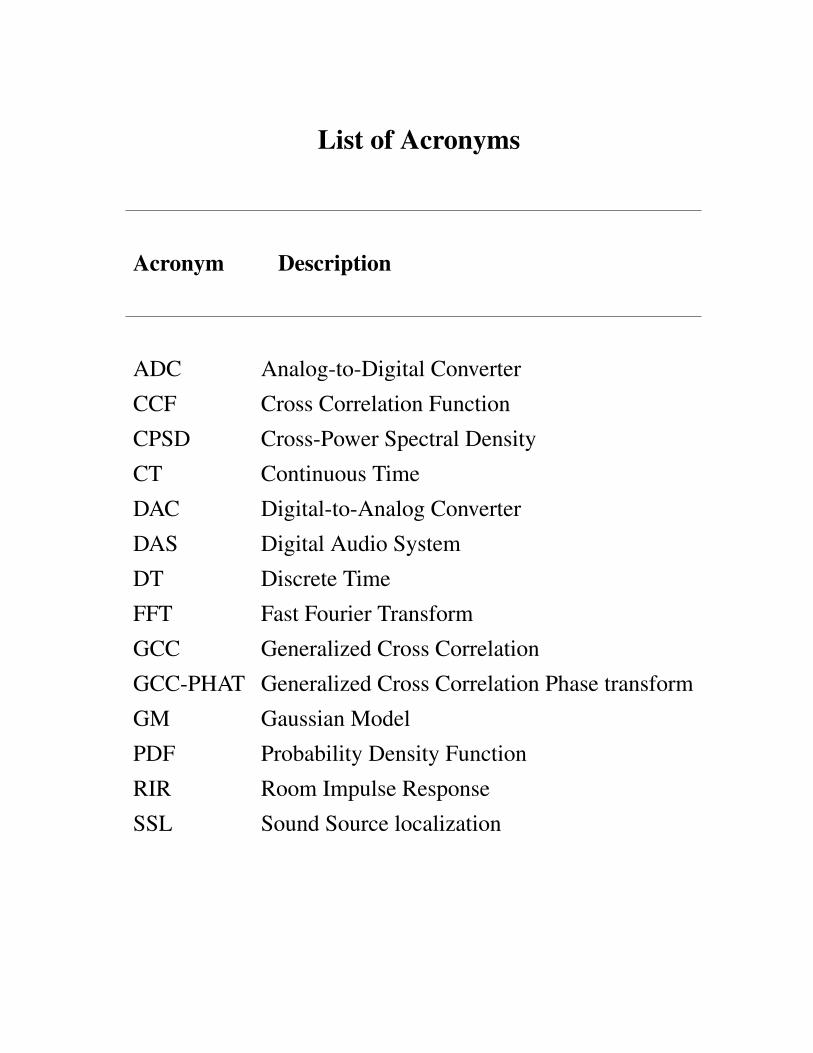
List of Acronyms

Acronym Description

ADC Analog-to-Digital Converter

CCF Cross Correlation Function

CPSD Cross-Power Spectral Density

CT Continuous Time

DAC Digital-to-Analog Converter

DAS Digital Audio System

DT Discrete Time

FFT Fast Fourier Transform

GCC Generalized Cross Correlation

GCC-PHAT Generalized Cross Correlation Phase transform

GM Gaussian Model

PDF Probability Density Function

RIR Room Impulse Response

SSL Sound Source localization

Chapter 1

Introduction

Sound Source Localization

History

Motivation

Problem Description

Thesis Organization

Chapter 1

Introduction

1.1 Sound Source Localization

Hearing, one of the primary sensors of a human body, is also one of the mostimportant gateways to the mind. Therefore, the fascination with sound andhearing is almost as old as recorded history. Sound engineering as a whole hasbeen a subject of interest to both scientific and music community. The particu-lar aspect sound detection and localization has been of greater significance to aresearch community for the alternatives that it provides in contrast to burdenedRF domain. Apparently, the medium of RF and sound are two orthogonal car-rier mediums in nature with respect to propagation, frequency of operation andscope of application. The constraints of RF spectrum with respect to bandwidthregulation and RF pollution provide an impetus to explore sound like a viablealternative in as many applications as possible.

Sound source localization (SSL) is crucial to most microphone array ap-plications such as speech enhancement [2], hands-free speech recognition [3],video-conferencing [4], and human-computer interface [5]. Many methods forSSL using microphone arrays have given in the literature [6]. For instance,distributed microphone network [7] and blind multiple-input multiple-outputfiltering [8] have been used to localize a sound source. Energy measurements

2

Chapter 1. Introduction

based method is given in [9]. Algorithms based on particle filtering are usedto locate and track a wideband acoustic source [10,11]. In practice, the mostpopular methods are the time-difference-of-arrival (TDOA) estimation meth-ods [12], such as adaptive eigenvalue decomposition (AED) [13] and general-ized cross-correlation phase transform (GCC-PHAT) [14]. It has been shownthat the method based on steered response power (SRP) is more robust thanthat based on time-difference-of arrival estimation. One of the most popularmodern localization algorithms is the steered response power using the phasetransform (SRP-PHAT) [16], also known as global coherence field (GCF) [15].

Localization methods can be divided into active and passive methods. Ac-tive methods send and receive energy whereas passive methods only receiveenergy. Active methods have the advantage of controlling the signal they emitwhich helps the reception process. Drawbacks of an active method include thatthe emitter position is revealed, more sophisticated transducers are required,and the energy consumption is higher compared to passive systems. As com-pared to active methods, Passive methods are more suitable for surveillancepurposes since no energy is intentionally emitted. This thesis focuses on pas-sive acoustic source localization methods.

1.2 History

Localization has been an important task in the history of mankind. In the be-ginning of modern navigation, one could determine his/her position at sea bymeasuring the angles from the horizon of celestial objects at a known time.The angles were determined via measurements, e.g., using a sextant. The ce-lestial objects angle above the horizon at a particular time determines a lineof position (LOP) on a map. The crossing of LOPs is the location. Modernnavigation and localization utilize mainly electromagnetic signals. The appli-cations of localization include radio detecting and ranging (RADAR) systems,

3


global positioning system (GPS) navigation, and light amplification by stim-ulated emission of radiation (LASER) -based localization technology. Othermeans of localization include utilization of sound waves in, e.g., underwaterapplications such as the sound navigation and ranging (SONAR).

1.3 Motivation

The main motivation of acoustic source localization is fuelled by the contribu-tion it plays in a number of applications such as robot processing, automaticvideo camera shooting in video conferences, hands free mobile communica-tions in the enclosed areas, and much more related applications. The Indianmilitary, in particular, the army, has been engaged in border monitoring, a factthat has warranted untiring deployment of military resources of human capitaland material. The primary aim of such deployment towards border monitoringis to detect enemy intrusion with an aim to counteract and pre-empt snow-balling situations by checking intrusion at an early stage. Typically, across aborder, gun firing is a typical phenomenon and many a times, the directionof these gun shots reveal vital information about adversaries. Currently, thesecurity forces do not employ any sensor setup to detect events with acousticemissions. In the event of a concrete and a fairly accurate acoustic detectionsystem, the task of monitoring would significantly ease on requirement of menand material in that the manpower can be channelized in specific direction andarea of interest rather than a general deployment spanning across the entirearea. This would mitigate the stress and the logistic pressure as well. This needmotivated the academic interest in this field to explore the feasibility of an endproduct based on the acoustic detection.

4


1.4 Problem Description

The process of sound source localization (SSL) is illustrated in fig 1.1. The SSLproblem is divided into four stages: sound emission, propagation, measure-ment, and localization. The first three stages represent the physical phenomenaand the measurement taking place before the localization algorithm solves thesource location. These stages are briefly discussed in the following subsections.This thesis focuses on the last stage and discusses signal processing methodsto locate the sound source. When discussing solutions to a problem, it is usefulto classify the type of problem. The prediction of results from measurementsrequires:1. A model of the system under investigations, and2. A physical theory linking the parameter of the model to the parameter beingmeasured.

A forward problem is to predict the measurement parameter from the modelparameter, which is often straightforward. An inverse problem uses measure-ment parameter to infer model parameters. An example of the forward problemwould state: output the received signal at the given microphone location by us-ing the known source location and the source signal. Assuming a free-fieldscenario, this would be achieved by simply delaying the source signal by theamount of sound propagation delay between source and microphone positionand attenuating the signal relative to the propagation path length. The inverseproblem would state: solve the source location by using the measured micro-phone signals at known locations. The example inverse problem is much moredifficult to answer than the forward problem. Hadamards definition of a well-posed problem is:1. A solution exists2. The solution is unique

5


3. The solution depends continuously on the dataA problem that violates one or more of these rules is termed ill-posed. Dur-

ing this thesis, it will become evident that sound source localization is an ill-posed inverse problem in most of the realistic scenarios.

1.5 Thesis Organization

This thesis consists of a total of six chapter organized as below :Chapter 1 : This chapter gives a brief introduction to the sound source lo-calization techniques in different environment and various applications of thesound source localization.Chapter 2: This chapter will give some basics of audio and speech processing,which includes capturing and converting the audio signal, segmentation andwindowing function etc.Chapter 3: This chapter will give the overview of the sound source localizationusing Naive-Bayes and Euclidean distance classifier.Chapter 4: This chapter will describe the implementation part of the SSL sys-tem.Chapter 5:The localization accuracy of the SSL system and the dependency ofit on various parameters are presented in this chapter.Chapter 6: This chapter will discuss the conclusion and the future work.

6

Chapter 2

Audio and Speech Processing

Introduction

Capturing and Converting Sound

Noise

Signal

Sampling

Segmentation

Window Functions

Chapter 2

Audio and Speech Processing

2.1 Introduction

Audio and speech processing systems have steadily risen in importance in theeveryday lives of most people in developed countries. From Hi-Fi music sys-tems, through radio to portable music players, audio processing is firmly en-trenched in providing entertainment to consumers. Digital audio techniques inparticular have now achieved a domination in audio delivery, with CD players,Internet radio, MP3 players and iPods being the systems of choice in manycases. Even within television and film studios, and in mixing desks for liveevents, digital processing now predominates. Music and sound effects are evenbecoming more prominent within computer games. Speech processing hasequally seen an upward worldwide trend, with the rise of cellular communi-cations, particularly the European GSM (Global System for Mobile communi-cations) standard. GSM is now virtually ubiquitous worldwide, and has seentremendous adoption even in the worlds poorest regions.

8

Chapter 2. Audio and Speech Processing

2.2 Capturing and Converting Sound

Either sound created through the speech production mechanism or sound asheard by a machine or human, is a longitudinal wave which travels through air(or a transverse wave in some other media) due to the vibration of molecules. Inair, sound is transmitted as a pressure variation, between high and low pressure,with the rate of pressure variation from low, to high, to low again, determiningthe frequency. The degree of pressure variation (namely the difference betweenthe high and the low) determines the amplitude.

A microphone captures sound waves, often by sensing the deflection causedby the wave on a thin membrane, transforming it proportionally to either volt-age or current. The resulting electrical signal is normally then converted to asequence of coded digital data using an analogue-to-digital converter (ADC).

If this same sequence of coded data is fed through a compatible digital-to-analogue converter (DAC), through an amplifier to a loudspeaker, then asound may be produced. In this case the voltage applied to the loudspeakerat every instant of time is proportional to the sample value from the computerbeing fed through the DAC. The voltage on the loudspeaker causes a coneto deflect in or out, and it is this cone which compresses (or rarifies) the airfrom instant to instant thus initiating a sound wave. In fact the process, shown

Figure 2.1: Block diagram of Digital Audio System

diagrammatically in figure 2.1, identifies the major steps in any digital audioprocessing system. Audio, in this case speech in free air, is converted to an

9


electrical signal by a microphone, amplified and probably filtered, before beingconverted into the digital domain by an ADC. Once in the digital domain, thesesignals can be processed, transmitted or stored in many ways, and indeed maybe experimented upon using Matlab. A reverse process will then convert thesignals back into sound.

2.3 Noise

Noise: Recorded sound is a combination of desired and undesired signals. Thespeech signal, we like to record is Desired signal; undesired signals includeechoes, environment noise, and other speech signals.

2.3.1 Statistical Property

In the time domain, a noise signal has a good statistical model called a zero-mean Gaussian process N(µN,σ

2N), with a known variance σ2

N and mean µN

p(y|µN) =1√

2πσNexp

(−(y−µN)

2

2σ2N

)(2.1)

p(y) =1√

2πσNexp(− y2

2σ2N

)(2.2)

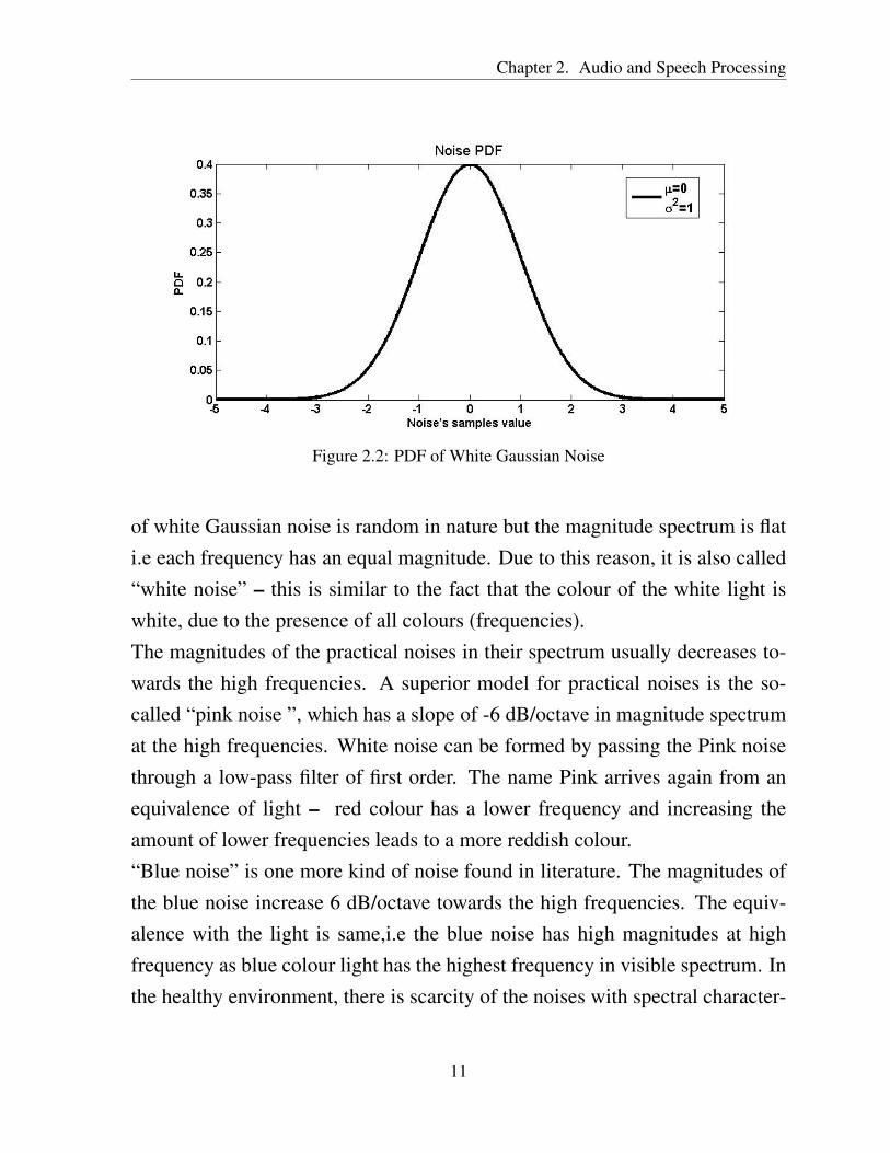
The noise signals can be well described by the single variable (σN) Gaussianmodel (2.2). Figure (2.2) depicts the PDF of a noise, which is symmetricalabout the mean µ = 0 and has standard deviation σ = 1.

2.3.2 Spectral Property

Noise has a special kind of property which signifies each frequency containshow much power, is known as “Power spectral density” . The phase spectrum

10


Figure 2.2: PDF of White Gaussian Noise

of white Gaussian noise is random in nature but the magnitude spectrum is flati.e each frequency has an equal magnitude. Due to this reason, it is also called“white noise” – this is similar to the fact that the colour of the white light iswhite, due to the presence of all colours (frequencies).The magnitudes of the practical noises in their spectrum usually decreases to-wards the high frequencies. A superior model for practical noises is the so-called “pink noise ”, which has a slope of -6 dB/octave in magnitude spectrumat the high frequencies. White noise can be formed by passing the Pink noisethrough a low-pass filter of first order. The name Pink arrives again from anequivalence of light – red colour has a lower frequency and increasing theamount of lower frequencies leads to a more reddish colour.“Blue noise” is one more kind of noise found in literature. The magnitudes ofthe blue noise increase 6 dB/octave towards the high frequencies. The equiv-alence with the light is same,i.e the blue noise has high magnitudes at highfrequency as blue colour light has the highest frequency in visible spectrum. Inthe healthy environment, there is scarcity of the noises with spectral character-

11


istics same as blue noise.A more kind of noise with the same analogy is called “coloured noise ”, whichis a noise signal with a given magnitude spectrum (imitating a given colour)and random phases.

2.3.3 Temporal Property

One of the temporal properties of a noise signal assumes the noise is a station-ary signal. This means that its probability distribution function and statisticalproperties in the time domain and mean and amplitude variation in the fre-quency domain, do not change with time. Sometimes, temporal property isreferred to as “quasi-stationary ”, that is, the noise signal properties vary muchmore slowly than the other signal properties it is compared with.

2.3.4 Spatial Property

Spatial properties of a noise signal is given by the locations of the noise sources.In frequent cases, there is no firmly specified location of the noise source orthere are too many noise sources.. In practice, the reverberation spreads thedistinct location of the noise sources. Consequently, we are dealing with am-bient noise in most of the cases; that means, there are no noise sources withfirmly defined locations. In modelling, we can assume that the noise energycomes from every direction with equal probability, which is called “Isotropicambient noise ”.

2.4 Signal

A signal is the desired part of the mixture of sounds recorded from the micro-phone. Unless stated clearly, by signal we will mean human speech. Humanspeech is a complex signal which comprises – a sequence of silence, plosive,unvoiced, and voiced segments.

12


• Silence segments are used to separate words and phonemes and are an inte-gral part of human speech.• In the signal spectrum, plosive segments contain transient variations of highlydynamic in nature .•Unvoiced segments are noise-like turbulence, produced when the air is forcedat high speed through a constriction in the vocal tract while the glottis is heldopen. They are characterized predominantly by the form of their spectral en-velopes .• Voiced segments are defined by their fundamental frequency, called “pitch ”and its formants (harmonics). Basically, the pitch is the fundamental frequencyof the vibration of vocal cords. The male voice has pitch frequencies rangefrom 50 to 250 Hz, while female voice has pitch frequencies range from 120 to500 Hz.

2.5 Sampling

2.5.1 Process

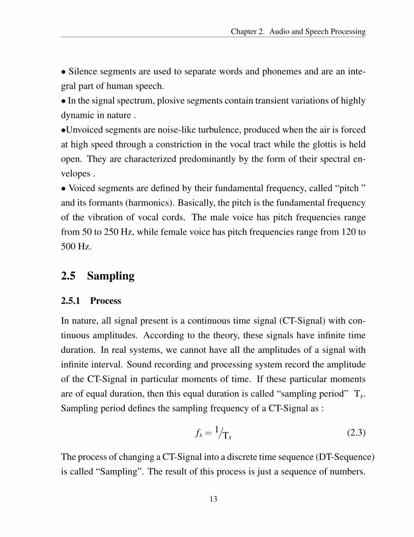
In nature, all signal present is a continuous time signal (CT-Signal) with con-tinuous amplitudes. According to the theory, these signals have infinite timeduration. In real systems, we cannot have all the amplitudes of a signal withinfinite interval. Sound recording and processing system record the amplitudeof the CT-Signal in particular moments of time. If these particular momentsare of equal duration, then this equal duration is called “sampling period” Ts.Sampling period defines the sampling frequency of a CT-Signal as :

fs = 1/Ts (2.3)

The process of changing a CT-Signal into a discrete time sequence (DT-Sequence)is called “Sampling”. The result of this process is just a sequence of numbers.

13


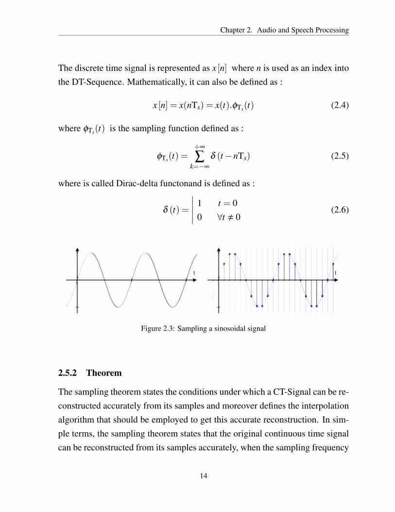
The discrete time signal is represented as x [n] where n is used as an index intothe DT-Sequence. Mathematically, it can also be defined as :

x [n] = x(nTs) = x(t).φTs(t) (2.4)

where φTs(t) is the sampling function defined as :

φTs(t) =+∞

∑k=−∞

δ (t−nTs) (2.5)

where is called Dirac-delta functonand is defined as :

δ (t) =

∣∣∣∣∣ 1 t = 00 ∀t , 0

(2.6)

Figure 2.3: Sampling a sinosoidal signal

2.5.2 Theorem

The sampling theorem states the conditions under which a CT-Signal can be re-constructed accurately from its samples and moreover defines the interpolationalgorithm that should be employed to get this accurate reconstruction. In sim-ple terms, the sampling theorem states that the original continuous time signalcan be reconstructed from its samples accurately, when the sampling frequency

14


fs is greater than the twice of the maximum frequency fm of the signal (seen ascomposition of sinosoids) to be discritized. :

fs > 2 fm (2.7)

The sample-rate is also called the Nyquist frequency, in honour to Harry Nyquistwho also contributed a lot to sampling theory. When this condition arrives, wecan reconstruct the underlying CT-Signal accurately by a process known assinc-interpolation.

2.6 Segmentation

Segmentation is needed when any of the following are true:1. The audio is continuous (i.e. we cant wait for a final sample to arrive beforebeginning processing).2. The nature of the audio signal is continually changing, or short-term featuresare important (i.e. a tone of steadily increasing frequency may be observed bya smaller Fourier transform snapshot but would average out to white noise ifthe entire sweep is analysed at once).3. The processing applied to each block scales nonlinearly in complexity (i.e. ablock twice as big would be four or even eight times more difficult to process).4. In an implementation, memory space is limited (very common).5. It is desirable to spread processing over a longer time period, rather thanperforming it all at the end of a recording.6. Latency is to be minimised a common requirement for voice communicationsystems.

Segmentation into frames is a basic necessity for much audio processing asmentioned above, but the process of segmentation does have its own fair shareof problems. Consider an audio feature. By that I mean some type of sound that

15


is contained within a vector of samples. Now when that vector is analysed itmight happen that the feature is split into two: half resides in one audio frame,and the other half in another frame. The complete feature does not residesin any analysis window, and may have effectively been hidden. In this way,features that are lucky enough to fall in the middle of a frame are emphasisedat the expense of features which are chopped in half. When windowing isconsidered, this problem is exacerbated further since audio at the extreme endsof an analysis frame will be de-emphasised further. The solution to the lost-feature problem is to overlap frames.

2.7 Window Functions

Windows are the functions defined across the time record which are periodic intime record. They have starting and stoping value zero and are smooth functionin between.

Speech is non-stationary signal where properties change quite rapidly overtime. For most phonemes the properties of the speech remain invariant fora short period of time ( 5-100 ms). Thus for a short window of time, tradi-tional signal processing methods can be applied relatively successfully. Mostof speech processing in fact is done in this way: by taking short windows (over-lapping possibly) and processing them. The short window of signal like this iscalled “frame”. In the windowing corresponds to what is understoods in filterdesign as window-method.

2.7.1 Hanning Window as an Example

Hanning window is the most widely used window. It has an amplitude variationof about 1.5 dB and provides better selectivity.

A window function is defined by a vector of real numbers {wi} , i= 1,2, ..,N−1. It is used by multiplying the time series of any signal xi with the window

16


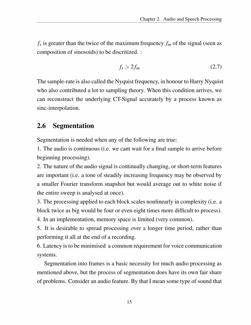
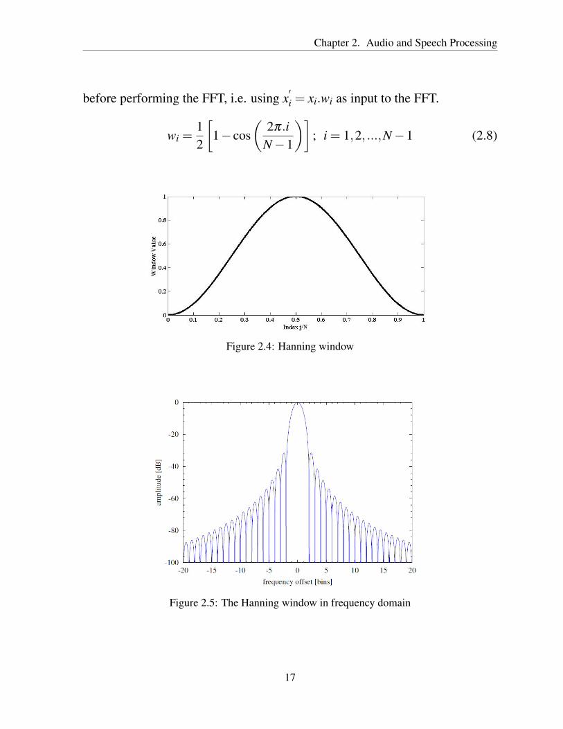
before performing the FFT, i.e. using x′i = xi.wi as input to the FFT.

wi =12

[1− cos

(2π.i

N−1

)]; i = 1,2, ...,N−1 (2.8)

Figure 2.4: Hanning window

Figure 2.5: The Hanning window in frequency domain

17

Chapter 3

System Overview

Introduction

Block Diagram Of Sound Source Localization

Description of the Block Diagram

Chapter 3

System Overview

3.1 Introduction

The sound source localization system, going to be overviewed here, is a clas-sification based localization system, in which location of sound source is esti-mated by one of the two classifier either Naive-Bayes classifier or Euclideandistance classifier.

3.2 Block Diagram of Sound Source Localization

The block diagram of Sound Source Localization (SSL) consists of two phases:1. Training phase2. Localization phase

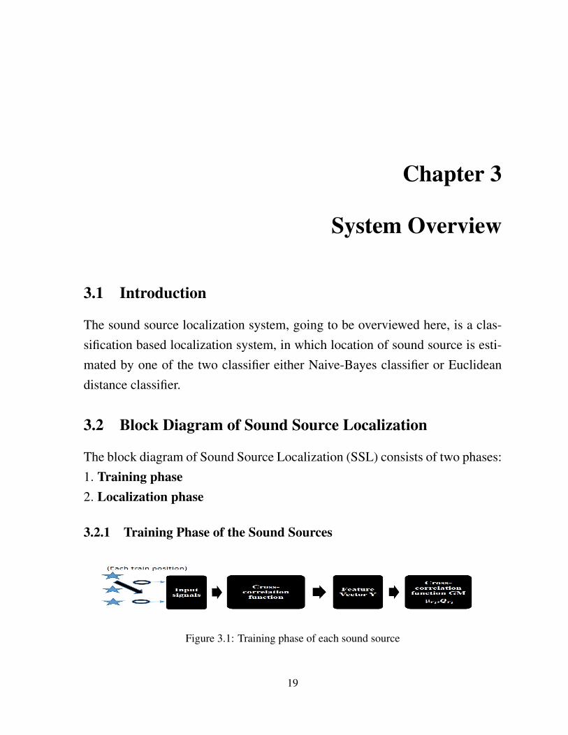
3.2.1 Training Phase of the Sound Sources

Figure 3.1: Training phase of each sound source

19

Chapter 3. System Overview

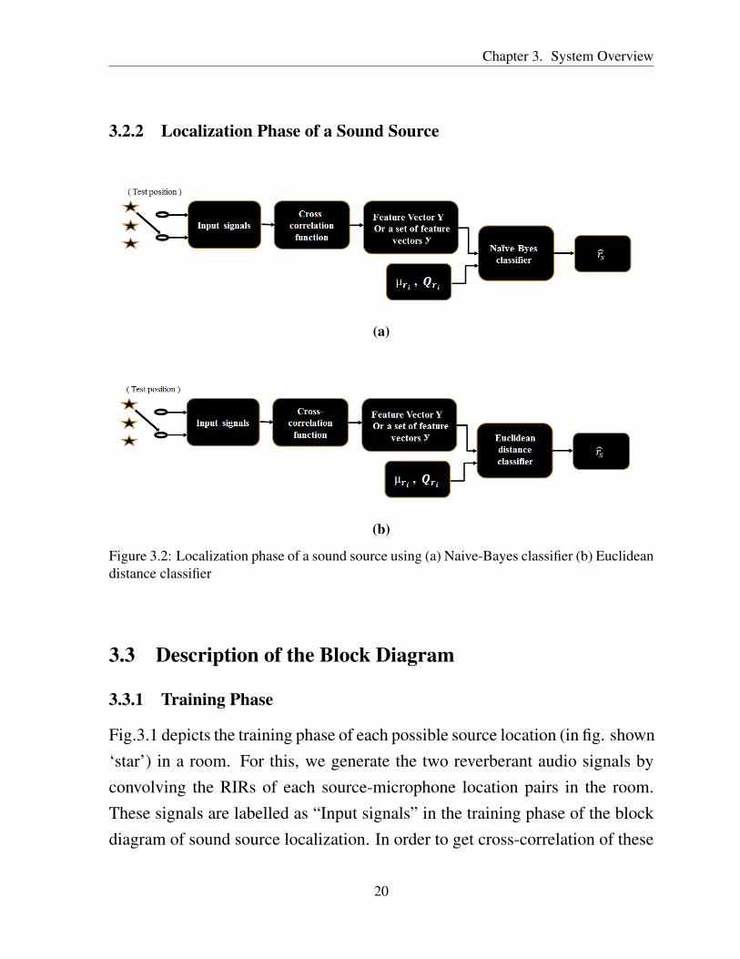
3.2.2 Localization Phase of a Sound Source

(a)

(b)

Figure 3.2: Localization phase of a sound source using (a) Naive-Bayes classifier (b) Euclideandistance classifier

3.3 Description of the Block Diagram

3.3.1 Training Phase

Fig.3.1 depicts the training phase of each possible source location (in fig. shown‘star’) in a room. For this, we generate the two reverberant audio signals byconvolving the RIRs of each source-microphone location pairs in the room.These signals are labelled as “Input signals” in the training phase of the blockdiagram of sound source localization. In order to get cross-correlation of these

20


two signals, we use generalized cross-correlation-phase transform method. Now,a feature vector Y is formed from the cross-correlated data. At the last, for eachsource location, mean vector and covariance matrix of cross–correlation func-tions are calculated and store to use in localization phase.

3.3.2 Localization Phase

Fig.3.2 depicts the localization phase of a sound source present in the room.When a reverberant signal (test data) comes from one of the trained locations,then the location of a source is estimated by discriminating the cross-correlationfunction. For this, the generalized cross-correlation function is calculated fromthe test data received at the microphones. Now, the feature vector (or a set of thefeature vectors, when N frames of test data availabe) is formed by selecting theproper range of delay parameter of the generalized cross-correlation function.The last stage of the localization is source location estimation using one of thetwo classifier : Naive-Bayes classifier and Euclidean distance classifier .

3.3.2.1 Source Location Estimation using Naive-Bayes Classifier

When Naive-Bayes algorithm is employed, the classifier gives a good soundsource location estimate based on the location lk that maximizes the probabilitydensity function plk

(ϒ).

Estimated sound source location∧ls using Naive-Bayes classifier is given by:

∧ls = argmax

lkplk

(ϒ) (3.1)

where plk(ϒ) is determind by the mean vector µlk and the covariance matrix

Clk .

21


3.3.2.2 Source Location Estimation using Euclidean Distance Classifier

When Euclidean distance algorithm is applied, the classifier gives a good soundsource location estimate based on the location that minimizes the Euclideandistance given in equation (4.24).

Estimated sound source location∧ls using Euclidean distance classifier is given

by:∧ls = argmin

lk

M

∑t=1

d2lk

(yt) (3.2)

where dlk(ϒi) is Euclidean distance

dlk

(yt)= ((yt−µlk

)T (yt−µlk))1/2

(3.3)

where “T ” for transpose operation.

22

Chapter 4

Implementation

Reverberant Speech Signal Model

Cross-Correlation Function

Localization Algorithms

Chapter 4

Implementation

4.1 Reverberant Speech Signal Model

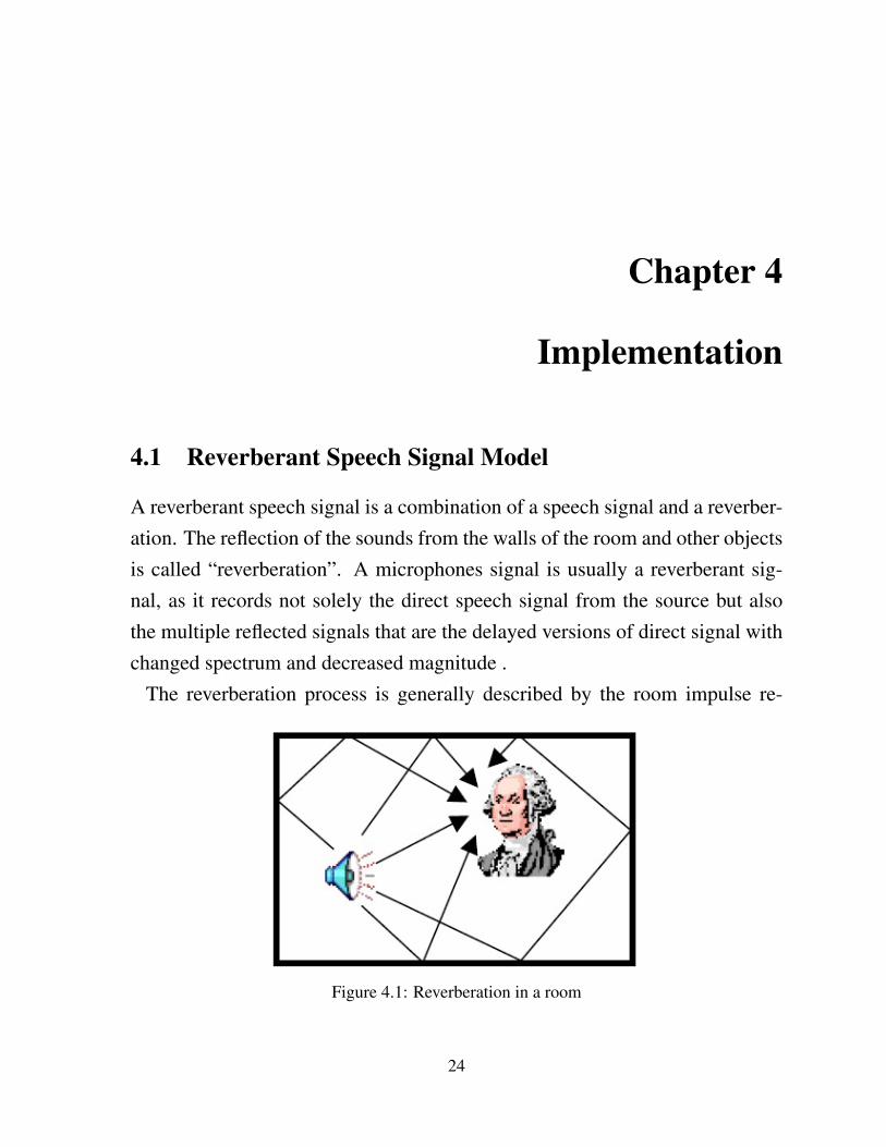
A reverberant speech signal is a combination of a speech signal and a reverber-ation. The reflection of the sounds from the walls of the room and other objectsis called “reverberation”. A microphones signal is usually a reverberant sig-nal, as it records not solely the direct speech signal from the source but alsothe multiple reflected signals that are the delayed versions of direct signal withchanged spectrum and decreased magnitude .

The reverberation process is generally described by the room impulse re-

Figure 4.1: Reverberation in a room

24

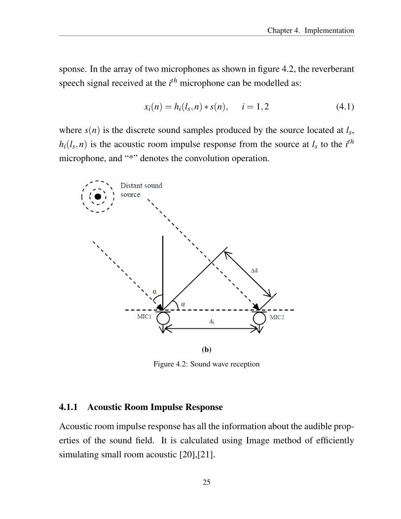
Chapter 4. Implementation

sponse. In the array of two microphones as shown in figure 4.2, the reverberantspeech signal received at the ith microphone can be modelled as:

xi(n) = hi(ls,n)∗ s(n), i = 1,2 (4.1)

where s(n) is the discrete sound samples produced by the source located at ls,hi(ls,n) is the acoustic room impulse response from the source at ls to the ith

microphone, and “*” denotes the convolution operation.

(b)

Figure 4.2: Sound wave reception

4.1.1 Acoustic Room Impulse Response

Acoustic room impulse response has all the information about the audible prop-erties of the sound field. It is calculated using Image method of efficientlysimulating small room acoustic [20],[21].

25


4.2 Cross-Correlation Function

The cross-correlation is a measure of similarity of two signals as a function ofthe delay of one with respect to the other. The peak value of cross-correlationfunction signifies the maximum similarity between the two signals at the certaindalay or lag, which is nothing but the delay between the two signals beingcompared.

(b)

Figure 4.3: Cross-correlation of the Sinosoidal signal with its delayed version

26


4.2.1 Determination of Cross-Correlation Function

The generalized CCF between the microphone-1′s signal x1(n) and the microphone-2′s signal x2(n) is determined in the freequency domain as :

Rx1x2 (τ) =

∞∫−∞

ρ1,2 (ω)X1 (ω)X∗2 (ω)e jωτdω (4.2)

where “*” denotes complex conjugation, ρ1,2 (ω) is the weighting function,and X1 (ω) and X2 (ω) are the Fourier transforms of the microphone signalsx1(t) and x2(t) respectively.In order to make generalized CCF less prone to reverberation, the phase trans-form method is used. By this method, the input signals are “whitened”, whichmeans the spectrum of input signals are uniformed with average magnitude.

ρ1,2 (ω) =1

|X1 (ω)X∗2 (ω) |(4.3)

Substituting (4.3) into (4.2), we have -

Rx1x2 (τ) =

∞∫−∞

X1 (ω)X∗2 (ω)

|X1 (ω)X∗2 (ω) |e jωτdω (4.4)

4.2.2 Features of Cross-Correlation Function

In practice, the microphone signals x1(t) and x2(t) are firstly windowed us-ing Hanning window (2.4), then the spectra X1(ω) and X2(ω) are calculatedthrough Fourier transforms applied to these windowed segments. From (4.1),if the window length is greater than the length of the room impulse response,the spectra of microphone signals can be expressed as :

Xi (ω) = Hi (ls,ω)S (ω) , i = 1,2 (4.5)

27


where S (ω) and Hi (ls,ω) are the Fourier transforms of s(n) and hi(ls,n) re-spectively.Substituting (4.5) into (4.4), we have -

Rx1x2 (τ) =

∞∫−∞

H1 (ls,ω)H∗2 (ls,ω)

|H1 (ls,ω)H∗2 (ls,ω) |e jωτdω = Rh1h2 (ls,τ) (4.6)

From (4.6), the generalized CCF of the input signals x1(n) and x2(n) is equalto that of the room impulse responses h1(ls,n) and h2(ls,n). However, since thewindow length is shorter than the length of the acoustic room impulse response,the microphone signals’ spectra are approximately expressed as :

Xi (ω)≈ Hi (ls,ω)S (ω) (4.7)

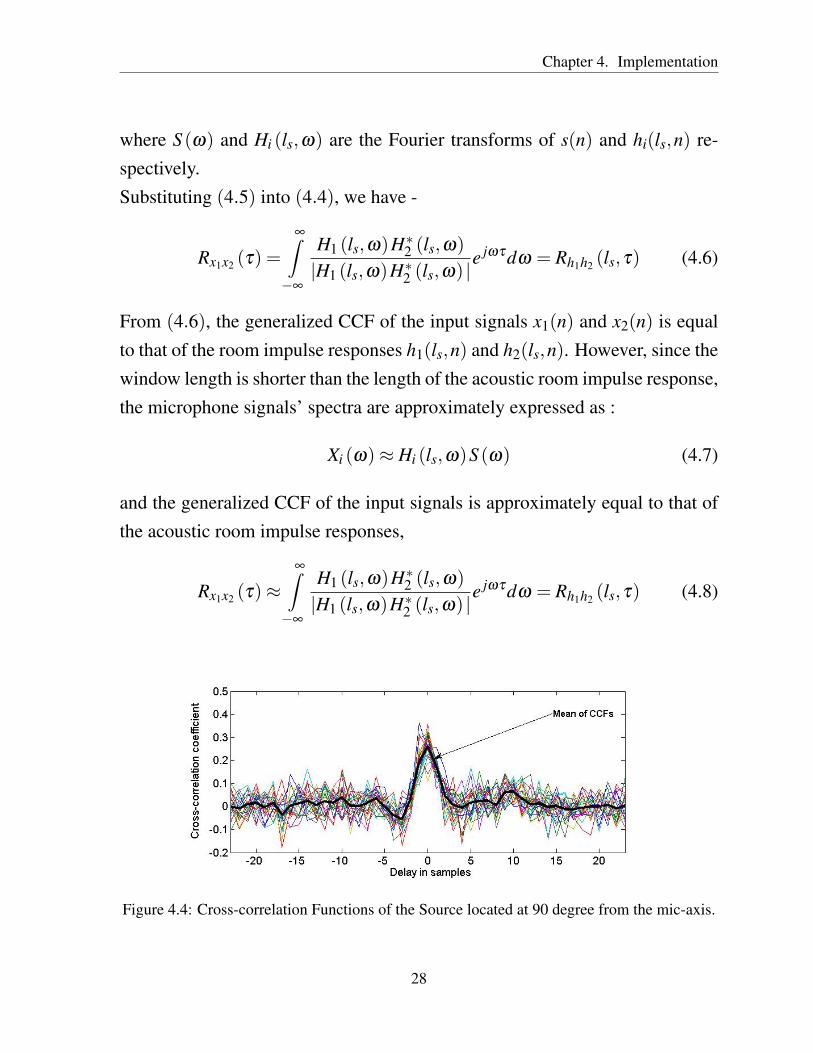
and the generalized CCF of the input signals is approximately equal to that ofthe acoustic room impulse responses,

Rx1x2 (τ)≈∞∫−∞

H1 (ls,ω)H∗2 (ls,ω)

|H1 (ls,ω)H∗2 (ls,ω) |e jωτdω = Rh1h2 (ls,τ) (4.8)

Figure 4.4: Cross-correlation Functions of the Source located at 90 degree from the mic-axis.

28


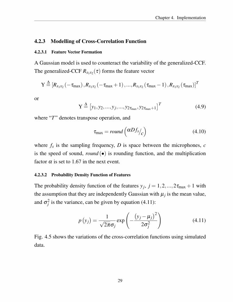
4.2.3 Modelling of Cross-Correlation Function

4.2.3.1 Feature Vector Formation

A Gaussian model is used to counteract the variability of the generalized-CCF.The generalized-CCF Rx1x2(τ) forms the feature vector

Y ∆= [Rx1x2 (−τmax) ,Rx1x2 (−τmax +1) , ...,Rx1x2 (τmax−1) ,Rx1x2 (τmax)]

T

orY ∆=[y1,y2, ...,y j, ...,y2τmax,y2τmax+1

]T (4.9)

where “T ” denotes transpose operation, and

τmax = round(

αD fs/c)

(4.10)

where fs is the sampling frequency, D is space between the microphones, c

is the speed of sound, round (•) is rounding function, and the multiplicationfactor α is set to 1.67 in the next event.

4.2.3.2 Probability Density Function of Features

The probability density function of the features y j, j = 1,2, ...,2τmax + 1 withthe assumption that they are independently Gaussian with µ j is the mean value,and σ2

j is the variance, can be given by equation (4.11):

p(y j)=

1√2πσ j

exp

(−(y j−µ j

)2

2σ2j

)(4.11)

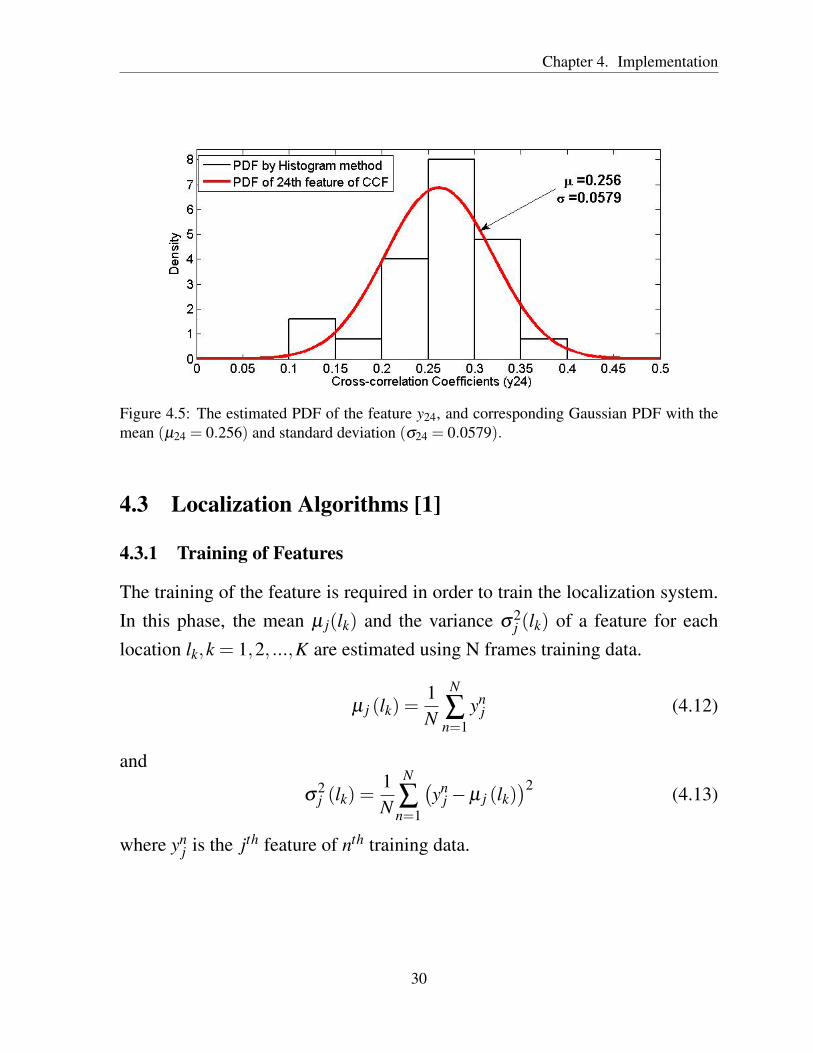
Fig. 4.5 shows the variations of the cross-correlation functions using simulateddata.

29


Figure 4.5: The estimated PDF of the feature y24, and corresponding Gaussian PDF with themean (µ24 = 0.256) and standard deviation (σ24 = 0.0579).

4.3 Localization Algorithms [1]

4.3.1 Training of Features

The training of the feature is required in order to train the localization system.In this phase, the mean µ j(lk) and the variance σ2

j (lk) of a feature for eachlocation lk,k = 1,2, ...,K are estimated using N frames training data.

µ j (lk) =1N

N

∑n=1

ynj (4.12)

and

σ2j (lk) =

1N

N

∑n=1

(yn

j−µ j (lk))2 (4.13)

where ynj is the jth feature of nth training data.

30


4.3.2 Testing or Localization Phase using Classifier

4.3.2.1 Naive-Bayes Classifier

The Naive-Bayes classifier assumes that each feature is statistically indepen-dent from the other features in order to estimate the source location. It uses afeature vector y or a group of feature vectors ϒ = {yt , t = 1, ....,M} of test datain order to estimate the location of the sound source using the mean vector µlk

and the covariance matrix Clk of the features from the training data.Using these data of each location lk i.e µlk and Clk , we can calculate the

PDF of each feature vector plk (y) of the test data as :

plk (y) =2τmax+1

∏j=1

plk(y j)=

2τmax+1

∏j=1

1√2πσ j (lk)

exp

(−(y j−µ j (lk)

)2

2σ2j (lk)

)or

plk (y) =1

(2π)(2τmax+1)/

2∣∣Clk

∣∣1/2 exp(−1

2(y−µlk

)TC−1lk

(y−µlk

))(4.14)

where∣∣Clk

∣∣ is the determinant of Clk . and

µlk =[

µ1 (lk) µ2 (lk) · · · µ2τmax+1 (lk)]

(4.15)

Clk =

σ2

1 (lk)

σ22 (lk)

. . .

σ22τmax+1 (lk)

(4.16)

In the case, when a group of the feature vectors ϒ= {yt , t = 1, ....,M} is present,

31


then the PDF of Y can be given as :

plk (ϒ)=M

∏t=1

plk(yt)= M

∏t=1

1

(2π)(2τmax+1)/

2∣∣Clk

∣∣1/2 exp(−1

2(yt−µlk

)TC−1lk

(yt−µlk

))(4.17)

plk (ϒ) =1

(2π)(2τmax+1)M/

2∣∣Clk

∣∣M/2 exp

(−1

2

M

∑t=1

(yt−µlk

)TC−1lk

(yt−µlk

))(4.18)

The last step is the estimation of sound source location∧ls using Naive-Bayes

classifier is given by:∧ls = argmax

lkplk

(ϒ) (4.19)

4.3.2.2 Euclidean Distance Classifier

The Euclidean distance classifier is employed, when the variances of each fea-ture are equal to σ2 for each location lk,k = 1,2, ...,K

σ2j (lk) = σ

2, j = 1,2, ...,2τmax +1 (4.20)

Substituting (4.20) into (4.16), the covariance matrix Clk can be rewritten as :

Clk =

σ2

σ2

. . .

σ2

2τmax+1×2τmax+1

(4.21)

Clk = σ2I (4.22)

32


where “I” represents the Identity matrix of order 2τmax +1.Substituting (4.22) into (4.18), we have -

plk (ϒ) =1

(2π)(2τmax+1)M/

2σM

exp

(− 1

2σ2

M

∑t=1

(yt−µlk

)T (yt−µlk))

or

plk (Y ) =1

(2π)(2τmax+1)M/

2σM

exp

(− 1

2σ2

M

∑t=1

d2lk

(yt)) (4.23)

where dlk (yt) is the Euclidean distance and is given by equation (4.24)-

dlk

(yt)= ((yt−µlk

)T (yt−µlk))1/2

(4.24)

The last step is the estimation of sound source location∧ls using Euclidean dis-

tance classifier is given by:

∧ls = argmin

lk

M

∑t=1

d2lk

(yt) (4.25)

33

Chapter 5

Simulation Results

Simulation Environment

Localization Accuracy

Dependency of Localization Accuracy

Accuracy Analysis

Chapter 5

Simulation Results

5.1 Simulation Environment

For simulation purpose, we have assumed a room of dimension 7× 6× 3mas shown in figure 5.1. The walls of the simulation room have a frequency-independent and uniform reflection coefficient that does not change with thechange in the direction or angle of the sound signal. The image method of

Figure 5.1: Simulation room

35

Chapter 5. Simulation Results

small room acoustic is used to generate the acoustic room impulse response.The positions of the two microphones are x1 = 3.85, y1 = 2.5, z1 = 1.2 and x2 =

4.15, y2 = 2.5, z2 = 1.2, where x, y, and z denotes the three different dimensionsof the simulation room (all in meters).The space between the two microphones is D = 0.3m and the radial distance ofthe speakers from the mid-point of the line joining the two microphones is 2m.

5.1.1 The Reverberant Speech Signal

The reverberant speech signals are made using “clean” speech and the acousticroom impulse response. When a “clean” speech signal is convolved with anacoustic room impulse response, then a reverberant signal is generated. Thesampling frequency of the “clean” speech is 16 khz.

5.1.2 Adding White Gaussian Noise

The additive white noise has a characteristic that it is uncorrelated with thedesired signal. Moreover, the additive Gaussian noises of the two microphonesare uncorrelated with each other. In order to get different signal-to noise ratio(SNR), the reverberant signals are added with the zero mean white Gaussiannoises of different variances. The SNRs of two microphones vary from 5 to 25dB.

5.1.3 Segmentation and Windowing

The frame size of each reverberant noisy signal is 512 samples (32 ms), andeach frame is windowed using a Hanning window given in equation (2.4).

5.1.4 Source Locations

We have considered seventeen speaker’s locations 10o, 20o, 30o, ......, 170o forboth training and testing.

36


5.2 Localization Accuracy

An outcome of a localization system is labelled as true estimate when the local-ization outcome is the true speaker’s location. The accuracy of a localizationsystem is defined as the percentage of true estimates over all the localizationestimates.

5.3 Dependency of Localization Accuracy

5.3.1 On the SNR and the Reverberation Time

Fig. 5.2 depicts the localization accuracy as a function of signal-to-noise ra-tio for the localization methods, where the number of training frames is 100 .As expected, at high signal-to-noise ratio levels, each of the methods performsvery well. But as reverberation time increases, the performances for both algo-rithms become bad .

(a) (b)

Figure 5.2: Accuracy of localization system for the Naive-Bayes and the Euclidean distancealgorithms with different SNR and Reverberation time (a) T60 = 0.3(s) (b) T60 = 0.6(s)

37


5.3.2 On the Number of Training Frames

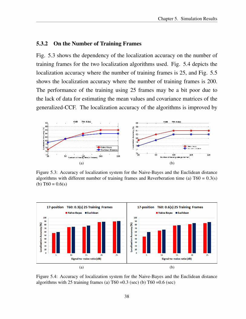
Fig. 5.3 shows the dependency of the localization accuracy on the number oftraining frames for the two localization algorithms used. Fig. 5.4 depicts thelocalization accuracy where the number of training frames is 25, and Fig. 5.5shows the localization accuracy where the number of training frames is 200.The performance of the training using 25 frames may be a bit poor due tothe lack of data for estimating the mean values and covariance matrices of thegeneralized-CCF. The localization accuracy of the algorithms is improved by

(a) (b)

Figure 5.3: Accuracy of localization system for the Naive-Bayes and the Euclidean distancealgorithms with different number of training frames and Reverberation time (a) T60 = 0.3(s)(b) T60 = 0.6(s)

(a) (b)

Figure 5.4: Accuracy of localization system for the Naive-Bayes and the Euclidean distancealgorithms with 25 training frames (a) T60 =0.3 (sec) (b) T60 =0.6 (sec)

38


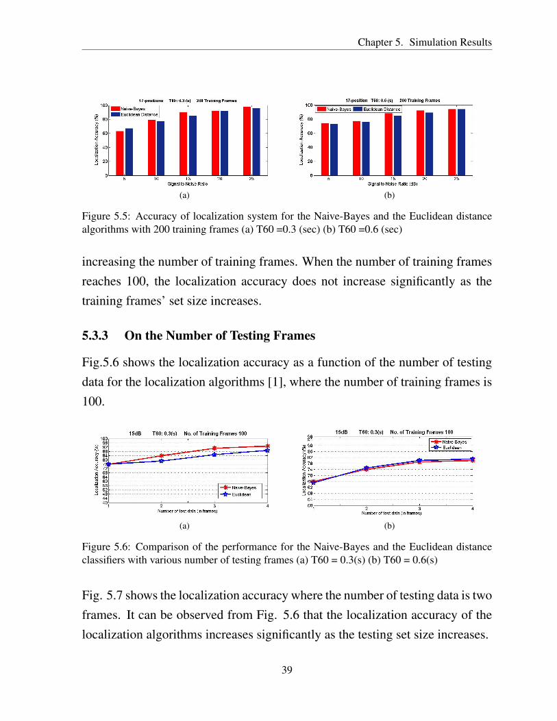
(a) (b)

Figure 5.5: Accuracy of localization system for the Naive-Bayes and the Euclidean distancealgorithms with 200 training frames (a) T60 =0.3 (sec) (b) T60 =0.6 (sec)

increasing the number of training frames. When the number of training framesreaches 100, the localization accuracy does not increase significantly as thetraining frames’ set size increases.

5.3.3 On the Number of Testing Frames

Fig.5.6 shows the localization accuracy as a function of the number of testingdata for the localization algorithms [1], where the number of training frames is100.

(a) (b)

Figure 5.6: Comparison of the performance for the Naive-Bayes and the Euclidean distanceclassifiers with various number of testing frames (a) T60 = 0.3(s) (b) T60 = 0.6(s)

Fig. 5.7 shows the localization accuracy where the number of testing data is twoframes. It can be observed from Fig. 5.6 that the localization accuracy of thelocalization algorithms increases significantly as the testing set size increases.

39


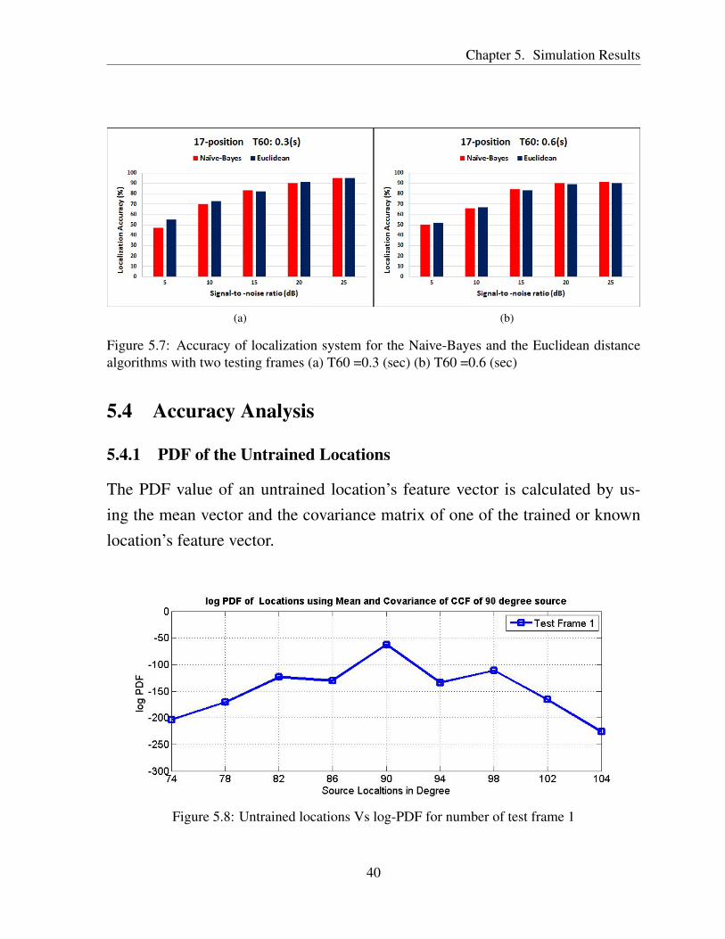
(a) (b)

Figure 5.7: Accuracy of localization system for the Naive-Bayes and the Euclidean distancealgorithms with two testing frames (a) T60 =0.3 (sec) (b) T60 =0.6 (sec)

5.4 Accuracy Analysis

5.4.1 PDF of the Untrained Locations

The PDF value of an untrained location’s feature vector is calculated by us-ing the mean vector and the covariance matrix of one of the trained or knownlocation’s feature vector.

Figure 5.8: Untrained locations Vs log-PDF for number of test frame 1

40


By finding the PDF values for each untrained location, we have evaluatedthe numerical values of PDF through simulation and presented the results infig. 5.8.

5.4.1.1 log-PDF Graph depends on the Number of Test Frame

Fig.5.9 shows the variation in log-PDF graph as a function of number of testframes. The difference between the log-PDF values of the trained location (90degree source) and the neighbour location (92 degree) increases as the numberof test frames increase. This increase in difference values of log-PDFs showsthat the probability of true estimate increases with increase in the number oftest frames.

Figure 5.9: Untrained locations Vs log-PDF for different number of test frames

5.4.1.2 log-PDF Graph depends on the Reverberation Time (T60)

Fig. 5.10 shows the variation in log-PDF graph as a function of Reverberationtime. The difference between the log-PDF values of the trained location (90degree source) and the neighbour location (92 degree) increases as the rever-beration time decreases. This increase in difference values of log-PDFs shows

41


Figure 5.10: Untrained locations Vs log-PDF for different T60

that the probability of true estimate increases with decrease in the reverberationtime.

5.4.2 Localization Accuracy of Naive-Bayes and Euclidean Distance Clas-sifiers

Fig. 5.11 shows the comparison of the two algorithms using log-PDF graph.

Figure 5.11: Comparison of Algorithms

42


It can be observed that the difference of log-PDF values of the trained andthe untrained location is greater for Naive-Bayes algorithm than that for theEuclidean distance algorithm. Hence, Naive-Bayes method is a better discrim-inator than the Euclidean distance method. Moreover, as the number of testframes increases the performance of the Naive-Bayes algorithm becomes betterthan that of the Euclidean distance algorithm since the difference of log-PDFvalue becomes larger for Naive-Bayes algorithm than for Euclidean distancealgorithm.

43

Chapter 6

Conclusion and Future work

Conclusion

Future work

Chapter 6

Conclusion and Future Work

6.1 Conclusion

We have simulated the SSL systems for both the algorithms [1] in MATLABplatform. These systems need the training of each location in a room, which isa very cumbersome process. In reverberant noisy environment, the localizationaccuracy of these systems is better than previous SRP-PHAT method basedsystem as given in [1]. To overcome training process of each location, we havetrained a particular location and in testing phase, we have calculated the PDFsof the feature vector using that trained location’s mean vector and covariancematrix and have plotted these PDFs for different locations. This graph may beuseful for the localization of untrained locations if we able to determine therelation between an untrained location’s PDF value and the trained location’sPDF value. The accuracy analysis for the two algorithms is presented in simu-lation results.

6.2 Future work

In our future work, we will try to locate the untrained locations by deriving therelation between the PDF of untrained locations and that of trained location.

45

Bibliography

[1] X. Wan and Z. Wu, “Sound source localization based on discrimination ofcross-correlation functions,” Applied Acoustics, vol. 74, no. 1, pp. 28–37,2013.

[2] J. Benesty, S. Makino, and J. Chen, Speech enhancement. Springer Sci-ence & Business Media, 2005.

[3] L. G. Brayda, C. Wellekens, M. Matassoni, and M. Omologo, “Speechrecognition in reverberant environments using remote microphones.,” inISM, pp. 584–591, 2006.

[4] M. Brandstein and D. Ward, Microphone arrays: signal processing tech-

niques and applications. Springer Science & Business Media, 2001.

[5] S. T. Shivappa, M. M. Trivedi, and B. D. Rao, “Audiovisual informationfusion in human–computer interfaces and intelligent environments: A sur-vey,” Proceedings of the IEEE, vol. 98, no. 10, pp. 1692–1715, 2010.

[6] J. P. Dmochowski and J. Benesty, “Steered beamforming approaches foracoustic source localization,” in Speech Processing in Modern Communi-

cation, pp. 307–337, Springer, 2010.

[7] G. Valenzise, G. Prandi, M. Tagliasacchi, and A. Sarti, “Resource con-strained efficient acoustic source localization and tracking using a dis-tributed network of microphones,” in Acoustics, Speech and Signal

46

Bibliography

Processing, 2008. ICASSP 2008. IEEE International Conference on,pp. 2581–2584, IEEE, 2008.

[8] A. Lombard, H. Buchner, and W. Kellermann, “Multidimensional local-ization of multiple sound sources using blind adaptive mimo system iden-tification,” in Multisensor Fusion and Integration for Intelligent Systems,

2006 IEEE International Conference on, pp. 7–12, IEEE, 2006.

[9] K. Ho and M. Sun, “An accurate algebraic closed-form solution forenergy-based source localization,” Audio, Speech, and Language Process-

ing, IEEE Transactions on, vol. 15, no. 8, pp. 2542–2550, 2007.

[10] D. B. Ward, E. A. Lehmann, and R. C. Williamson, “Particle filtering al-gorithms for tracking an acoustic source in a reverberant environment,”Speech and Audio Processing, IEEE Transactions on, vol. 11, no. 6,pp. 826–836, 2003.

[11] Z. Liang, X. Ma, and X. Dai, “Robust tracking of moving sound sourceusing scaled unscented particle filter,” Applied Acoustics, vol. 69, no. 8,pp. 673–680, 2008.

[12] J. Chen, J. Benesty, and Y. Huang, “Time delay estimation in room acous-tic environments: an overview,” EURASIP Journal on applied signal pro-

cessing, vol. 2006, pp. 1–19, 2006.

[13] J. Benesty, “Adaptive eigenvalue decomposition algorithm for passiveacoustic source localization,” The Journal of the Acoustical Society of

America, vol. 107, no. 1, pp. 384–391, 2000.

[14] C. Knapp and G. Carter, “The generalized correlation method for estima-tion of time delay,” IEEE Trans Acoust Speech Signal Process, vol. 24,no. 4, pp. 320–327, 1976.

47

Bibliography

[15] A. Brutti, M. Omologo, and P. Svaizer, “Comparison between differentsound source localization techniques based on a real data collection,”in Hands-Free Speech Communication and Microphone Arrays, 2008.

HSCMA 2008, pp. 69–72, IEEE, 2008.

[16] J. DiBiase, H. Silverman, and M. Brandstein, “Microphone arrays. robustlocalization in reverberant rooms,” Microphone Arrays: Signal Process-

ing Techniques and Applications, 2001.

[17] X. Wan and Z. Wu, “Improved steered response power method for soundsource localization based on principal eigenvector,” Applied Acoustics,vol. 71, no. 12, pp. 1126–1131, 2010.

[18] A. Brutti, M. Omologo, P. Svaizer, and C. Zieger, “Classification of acous-tic maps to determine speaker position and orientation from a distributedmicrophone network,” in Acoustics, Speech and Signal Processing, 2007.

ICASSP 2007. IEEE International Conference on, vol. 4, pp. IV–493,IEEE, 2007.

[19] N. Strobel and R. Rabenstein, “Classification of time delay estimates forrobust speaker localization,” in Acoustics, Speech, and Signal Process-

ing, 1999. Proceedings., 1999 IEEE International Conference on, vol. 6,pp. 3081–3084, IEEE, 1999.

[20] J. Allen and D. Berkley, “Image method for efficiently simulating small-room acoustics,” J Acoust Soc Am, vol. 65, no. 4, pp. 943–50, 1979.

[21] S. McGovern, Room Impulse Response Generator.http://in.mathworks.com/matlabcentral/fileexchange/5116-room-impulse-response-generator.

48

Documents

Accuracy Analysis of Sound Source Localization using Cross ...ethesis.nitrkl.ac.in/7257/1/Accuracy_Yadav_2015.pdf · Sound Source Localization using Cross-correlation of Signals from