Embed Size (px)
Citation preview
Accuracy in Parameter Estimation for Targeted Effects in StructuralEquation Modeling: Sample Size Planning for Narrow Confidence Intervals
Keke Lai and Ken KelleyUniversity of Notre Dame
In addition to evaluating a structural equation model (SEM) as a whole, often the model parameters areof interest and confidence intervals for those parameters are formed. Given a model with a good overallfit, it is entirely possible for the targeted effects of interest to have very wide confidence intervals, thusgiving little information about the magnitude of the population targeted effects. With the goal ofobtaining sufficiently narrow confidence intervals for the model parameters of interest, sample sizeplanning methods for SEM are developed from the accuracy in parameter estimation approach. Onemethod plans for the sample size so that the expected confidence interval width is sufficiently narrow. Anextended procedure ensures that the obtained confidence interval will be no wider than desired, with somespecified degree of assurance. A Monte Carlo simulation study was conducted that verified the effec-tiveness of the procedures in realistic situations. The methods developed have been implemented in theMBESS package in R so that they can be easily applied by researchers.
Keywords: structural equation modeling, sample size planning, confidence interval, accuracy inparameter estimation, power analysis
Structural equation modeling (SEM) is a widely used method inthe behavioral, educational, social, and managerial sciences, wherevariables are measured with error and/or latent constructs aretheorized to exist (for reviews of SEM, see, e.g., Bentler &Dudgeon, 1996; Bollen, 2002; MacCallum & Austin, 2000). Stud-ies that use SEM generally evaluate the performance of the hy-pothesized model with chi-square likelihood ratio tests and/or fitindices. For example, if the overall model fit is of interest, achi-square test can be performed to examine whether the nullhypothesis H0: � � �(�) can be rejected at the designated signif-icance level, where � is the population covariance matrix of themanifest variables and �(�) is the population model-implied co-variance matrix. If a specific part of the model (e.g., a direct pathfrom one latent variable to another, the covariance between twolatent variables, a factor loading) is of interest, one can conduct aWald test or a likelihood ratio test to probabilistically infer if thenull hypothesis that those specific paths are zero can be rejected(for statistical theories of Wald test and likelihood ratio test ap-plied to SEM, see, e.g., Mulaik, 2009, pp. 373–381).
However, as has been echoed many times in the literature, thereare limitations to null hypothesis significance tests (NHSTs; see,e.g., Nickerson, 2000, which provides a comprehensive historicalreview; see also Cohen, 1994; Meehl, 1997; Schmidt, 1996). Manytimes, even before conducting NHST, it is known from substantivetheories and experience that the null hypothesis is almost certainlyfalse. For example, the correlation between two exogenous vari-
ables is almost certainly not zero for many psychological con-structs, but a null hypothesis that the correlation is zero is usuallytested anyway. Admittedly, NHST informs researchers of thedirectionality of the population effect and thus helps to understandthe phenomenon under study (e.g., if the null value of zero,without loss of generality, is rejected, the population effect isinferred to be either positive or negative). However, the results ofa dichotomous (reject or fail-to-reject) significance test should notbe the endpoint of scientific inquiry, because knowing whether thepopulation effect is larger than zero does not answer the questionabout the magnitude of the population effect, which is often ofultimate interest. It would better facilitate the cumulation ofknowledge of a discipline if studies also report plausible values forthe population effect size of interest, which can be fulfilled viaconfidence intervals (CIs). A CI indicates probabilistically not onlywhat the population parameter is not (i.e., those values excluded bythe CI) but a range of plausible values (i.e., those values containedwithin the CI), and thus generally provides more information thandoes NHST (for more detailed discussions on the differencesbetween CI and NHST, see, e.g., Harlow, Mulaik, & Steiger, 1997;Kelley & Maxwell, 2003; Kelley, Maxwell, & Rausch, 2003;Maxwell, Kelley, & Rausch, 2008).
Recent authoritative sources have urged that applied researchreport effect sizes and their corresponding CIs. For example, thePublication Manual of the American Psychological Association(American Psychological Association [APA], 2001) states that the“reporting of confidence intervals . . . for effect sizes . . . can be . . .extremely effective. . . . The use of confidence intervals is there-fore strongly recommended” (p. 22). Moreover, in the latest Pub-lication Manual (APA, 2010), the APA continues to increase itsstress on using CIs, by stating that NHST is “but a starting point”and additional reporting elements such as effect sizes and CIs arenecessary to “convey the most complete meaning of the results”and are “minimum expectations for all APA journals” (p. 33). In
This article was published Online First March 21, 2011.Keke Lai, Department of Psychology, University of Notre Dame; Ken
Kelley, Department of Management, University of Notre Dame.Correspondence concerning this article should be addressed to Ken
Kelley, Department of Management, University of Notre Dame, NotreDame, IN 46556. E-mail: [email protected]
Psychological Methods2011, Vol. 16, No. 2, 127–148
© 2011 American Psychological Association1082-989X/11/$12.00 DOI: 10.1037/a0021764
127
the same vein, the American Educational Research Association(2006) states in its research guidelines that, for each of the majorstatistical results, there should be (a) an effect size of some kindand (b) an indication of the uncertainty of that effect size estima-tion, such as a CI (p. 37). Similar arguments are also available inthe medical sciences (e.g., International Committee of MedicalJournal Editors, 2004) and physiology (e.g., Curran-Everett &Benos, 2004), among others.
Effect sizes in the SEM context can be categorized into twotypes: (a) omnibus effects, which refer to the fit of the model as awhole, such as the nonnormed fit index (Bentler & Bonett, 1980)and the root mean square error of approximation (Browne &Cudeck, 1992; Steiger & Lind, 1980); and (b) targeted effects,which refer to the effect of a specific part of the model, such as thecoefficient of a structural path, the covariance between two latentvariables, or a factor loading. In addition to evaluating the fit of themodel as a whole, many times a specific part of the model is alsoof interest. Moreover, a finding of a good overall fit does not implythat the targeted effects of interest are strong and/or practicallyimportant. It is possible for such effects to be weak or even trivialin a model with a good overall fit, if the dynamics in the model arein fact instead explained by large residual variances for endoge-nous variables (MacCallum & Austin, 2000). Therefore, it iscritically important to study the targeted effects in a model so thatthe researcher can better understand the strength of the specificrelationships of interest and evaluate substantive theories. Toachieve this goal, instead of performing the traditional NHST toinfer if some path coefficients and/or covariances or correlationsequal zero, CIs can be formed, because CIs can convey not onlythe direction but the magnitude of the population parameters ofinterest.
Whenever an interval estimate is of interest, all other thingsbeing equal, it is more desirable to observe a narrow CI, ascompared with a wider one, because a narrow CI includes anarrower range of plausible parameter values and thus is moreinformative. Congruent with the increasing emphasis on reportingCIs for effect sizes, a study can be designed with the goal ofobtaining a narrow CI. Planning the sample size for a study withthe goal of obtaining a narrow CI dates back to at least Guenther(1965) and Mace (1964), and is becoming popular recently as analternative to, or supplement for, power analysis, as a result of theincreasing emphasis on effect size estimation and CI formation.This approach to sample size planning has been set in a frameworktermed accuracy in parameter estimation (AIPE; e.g., Kelley,2007c, 2008; Kelley & Maxwell, 2003; Kelley & Rausch, 2006),where the goal is to achieve a sufficiently narrow CI so that theparameter estimate will have a high degree of expected accuracy(for a review of applications of AIPE, see Maxwell et al., 2008).The desired CI width depends on the goals of the study and isdetermined by the researcher on a case-by-case basis, much likesetting the desired level of statistical power if one was planningsample size from the power approach.
Throughout this article, we emphasize the input–output rela-tionship of the sample size planning procedure. The input in thepresent context is usually a set of presumed population values. Thefocus of the present article is to show, given a certain set of inputspecifications, how to calculate the necessary sample size (i.e.,output). To what extent the sample size calculated is approximate(i.e., the CI width obtained in a study compared with the desired
width) depends on the quality of the input. To help estimate thenecessary input values, we then propose several practical methodsas a supplement to the literature review, which is generally theprimary source for estimating the input parameters.
The present article develops methods to plan sample sizes fortargeted effects in SEM so that the CIs for the parameters ofinterest will be sufficiently narrow. The standard method plans forthe sample size so that the expected value of a CI width will be nolarger than desired. Because the CI width is a random variable,setting the expected width to be sufficiently narrow does notguarantee that a CI observed in a particular study will be suffi-ciently narrow. This standard method is extended so that the CIobtained in a particular study will be no wider than desired, withsome specified, usually high (e.g., 80%, 90%, 99%), degree ofassurance. Because the sample size planning methods are based onstandard CI formation methods in the existing SEM literature,which are technically approximate (i.e., based on asymptotic dis-tributions but used at finite sample sizes), a Monte Carlo simula-tion study is conducted to evaluate the effectiveness of the pro-posed sample size planning methods. These sample size planningmethods have been implemented in specialized R functions (RDevelopment Core Team, 2010) in the MBESS package (Kelley,2007a, 2007b; Kelley & Lai, 2010), so that they can be easilyapplied by researchers.1
CI Formation for SEM Model Parameters
There are several methods to construct CIs for SEM parameters;two of the most widely used are (a) maximum likelihood estima-tion (MLE; for a thorough discussion on likelihood methods, see,e.g., Pawitan, 2001; for applications in the SEM context, see, e.g.,Bollen, 1989) and (b) the bootstrap approach (Efron & Tibshirani,1993; for applications of the bootstrap to SEM, see Beran &Srivastava, 1985; Bollen & Stine, 1993; Yuan & Hayashi, 2006).Moreover, maximum likelihood standard errors can be based onthe expected information matrix, the observed information matrix,or a sandwich-type covariance matrix (e.g., Arminger & Schoen-berg, 1989; Bollen, 1989; Browne & Arminger, 1995; Shapiro,1983; White, 1982; Yuan & Hayashi, 2006). The present articlebases CI formation on the expected information matrix to developsample size planning methods, for the following reasons: (a) Othermethods require raw data and thus are not suitable for sample sizeplanning, which is necessarily performed before data collection;(b) almost all SEM programs (e.g., AMOS, EQS, LISREL, Mplus,SAS PROC CALIS, the sem package in R) use (at least by default)the expected information matrix to construct CIs; and (c) differentmethods tend to give similar CIs if the assumptions (e.g., multi-variate normality) are satisfied and the model is correctly specified.
We briefly review the CI formation in this section, because it isimportant when we formally present the sample size planningmethods. Detailed analytical derivation of the standard errors ofMLE for SEM model parameters is available in Yuan and Hayashi(2006). We developed the sample size planning methods based onthe inferential methods most commonly used in the SEM literature
1 MBESS was originally an acronym for Methods for Behavioral, Edu-cational, and Social Sciences, but is used as a stand-alone package titlenow.
128 LAI AND KELLEY
and by SEM software (i.e., maximum likelihood with the expectedinformation matrix). The performance of the sample size planningprocedures depends on the performance of the MLE, and in situ-ations where MLE is less effective, the sample size planned maybe different from the idealized sample size. Because maximumlikelihood techniques are based on the asymptotic properties ofthe estimation, at any finite sample size inferences given by MLEare technically approximate. Therefore, we empirically evaluatethe performance of our sample size planning procedures and MLEwith a Monte Carlo simulation study in a later section. It shouldbe made clear that the errors arising from using maximum likeli-hood asymptotic properties to approximate the behavior of MLE atfinite sample sizes exist in any situation where maximum likeli-hood is applied. Such errors are not caused by sample size plan-ning methods and are not unique to this article.
Let x1, x2, . . . , xn denote a random sample from a p-variatemultivariate normal distribution with population covariance matrix�. The present interest is to model the covariance matrix with aproposed structure, and the covariance matrix implied by themodel is denoted as �(�), where � is a vector containing the modelparameters. If the model is correct, that is, �(�) � �, andxi � N��, �) (i � 1, . . . , n), the log-likelihood function used to fitthe model is (e.g., Bollen, 1989, pp. 132–134)
l��� � �i�1
n
li���
� �n
2�ln��(�)� � tr�S�����1�� � c, (1)
where
li(�)��1
2ln������ �
1
2�xi � x��T�����1�xi � x�� � c�, (2)
S is the observed p � p covariance matrix based on a sample ofsize n, x� is the sample mean vector, and c and c� are constants thathave no influence on the choice of �.
Let �n denote the maximum likelihood estimator of � based ona sample of size n. Standard asymptotic theories state that �n, theMLE for �, converges in distribution to a multivariate normaldistribution as n 3 (e.g., Lehmann, 1998; Pawitan, 2001):
�n��n � ��L¡ N(0, I����1), (3)
where I(�) is the expected information matrix and can be consid-ered as the function I( ) evaluated at �. That is,
I��� � E�� li����� ���,
where li refers to the second derivative of the log-likelihood li (fordetailed discussion on MLE and the expected information matrix.see, e.g., Pawitan, 2001). However, the population parameter � isunknown, and thus I(�) is unknown and needs to be estimated.Because �n is a consistent estimator of �, �n converges in proba-bility to � as n 3 :
�nP¡ �. (4)
Under the commonly used assumption that the function I( ) isdifferentiable, plugging �n into I( ) leads to
I��n�P¡ I���. (5)
The assumption that I( ) is differentiable is a condition included inthe so-called regularity conditions (e.g., Lehmann, 1998; Pawitan,2001), which are commonly assumed in the literature when apply-ing MLE.
If one takes the sum of the information over n individuals andcalculates the mean, Equation 5 leads to
1
nIn��n�
P¡ I���, (6)
which states that the estimated expected information matrix con-verges in probability to the expected information matrix as n3 .Notice that the difference between Equations 5 and 6 is that In(�n)is the sum of information over n individuals, that is,
In��n� � E��i�1
n
� li ��������n,
whereas I(�n) is based on one observation, that is,
I��n� � E �� li ��������n.
Therefore, if one replaces I(�)�1 in Equation 3 with its estimate,at a given finite sample size n, �n approximately follows a multi-variate normal distribution with covariance matrix In(�n)�1:
�n N��, K�, (7)
where K � [kij] � In(�n)�1. Because In(�n)�1 � I(�n)�1/n,Equation 7 is equivalent to
�n N��, H/n�, (8)
where H � [hij] � I(�n)�1.After obtaining the approximate distribution of �n, it is now
possible to form CIs for model parameters of interest. Let �j, thejth element in �, denote the model parameter of interest. Becausemultivariate normality implies univariate normality for all vari-ables, �n following a multivariate normal distribution states that �j
at sample size n follows a normal distribution. Then the (1 � �)100% CI for �j is
CI�1��� � ��j � z1��/ 2�kjj � �j � �j � z1��/ 2�kjj�, (9)
or equivalently
CI�1��� � ��j � z1��/ 2�hjj
n� �j � �j � z1��/ 2�hjj
n �, (10)
where z1��/2 refers to the (1 � �/2)th quantile of the standardnormal distribution. In summary, the CI formation reviewed in thissection is based on MLE with expected information matrix andserves as the basis of our sample size planning methods.
129AIPE FOR TARGETED EFFECTS IN SEM
Accuracy in Parameter Estimation for SEMModel Parameters
Let w denote the full CI width obtained in a particular study. Let denote the desired CI width for the population parameter ofinterest, and it is specified by the researcher a priori according tothe purpose of the study. The concept of “sufficiently narrow” (i.e.,the value of ) is loosely defined in the present article, because thespecific value varies dramatically depending on at least (a) thegoals of the study, (b) the measurement unit of the variable ofinterest, and (c) the conventions in the particular area of study.Therefore, the desired CI width needs to be specified by theresearcher on a case-by-case basis. For example, if the study ismore confirmatory in nature, the researcher may generally plan toobtain a smaller value, whereas the researcher may be satisfiedwith a larger value in a study that is more exploratory in nature.For the reasons discussed above, sample size planning methods,both in the literature and in this article, focus on how to achieve thegoal w � instead of how to set the goal (i.e., the value of ).
We need to emphasize that there is no such thing as the correctwidth for a study. Given the purposes of a study, a (continuous)range of values may be considered as suitable, and this range cansometimes be quite large. Instead of asking how to choose thedesired CI width, sometimes it is easier for the researcher to startby precluding undesirable values. Because there is no “correct” value, any value is in fact reasonable as long as it does not makethe CI too wide to be informative. We also discuss a practicalmethod to facilitate the task of specifying value in a later section.
Planning Sample Size for the Expected CI Width toBe Sufficiently Narrow
Planning sample size from the AIPE perspective aims to find theminimum n such that w � . Because the realized width w is arandom variable, one approach is to aim at the expectation of wand obtain the minimum n so that E[w] � . Based on Equation10, the full CI width obtained is
w � 2z1��/ 2s � j � 2z1��/ 2�hjj
n, (11)
where s�j is the standard error for �j, the point estimate of the modelparameter of interest. Taking the expectation on both sides ofEquation 11 gives
E�w� � E�2z1��/ 2s� j�
� 2z1��/ 2E�s� j�
� 2z1��/ 2��j
� 2z1��/ 2�hjj
n. (12)
Although strictly speaking E�s�j� � ��j, the difference betweenthese two quantities is very trivial for typical sample sizes in theSEM context, and sample size planning can proceed using ��j asthe expectation of s�j.
2
The quantity hjj in Equation 12 is an element of H, which isequal to I(�)�1; to calculate I(�)�1, one can obtain I(�) first. If theproposed model is correct, that is, � � �(�), the expected infor-mation matrix I(�) can be obtained by fitting the model to thepopulation covariance matrix of manifest variables. More specif-ically, as discussed in the previous section of CI formation meth-ods, I(�) is the resulting matrix of evaluating the function I( ) at �,and therefore, to obtain I(�), it requires I( ) and �. The function I( )can be obtained by taking the expectation of the second derivativeof the log-likelihood function in Equation 1. Analytic derivationsto obtain the second derivative of the log-likelihood function areavailable in Yuan and Hayashi (2006). The values of � can beobtained by substituting � for S in the log-likelihood function inEquation 1. After I(�) is obtained, because H � I(�)�1, invertingI(�) gives H, which is the asymptotic covariance matrix of themultivariate normal distribution in Equation 3, or equivalently theasymptotic counterpart of H in Equation 8. Extracting the jjthcomponent of H gives hjj, which is the asymptotic variance of �j.Although the above steps to calculate hjj from � might soundtechnical, this task can be easily performed by almost any main-stream SEM software. If one uses the population covariance matrixof manifest variables to fit the model, the “standard error” for �j
returned by the software is in fact the population standard devia-tion �kjj. Then one can obtain hjj given the relation between K andH discussed above.3
Therefore, based on Equation 12, given �, which implies that hjj
is implicitly available, the CI width would depend only on thedesired confidence level (i.e., 1 � �) and n. The desired confidencelevel (e.g., .95) is generally considered a fixed factor, yet n canvary. Correspondingly, solving Equation 12 for n leads to thesmallest sample size that satisfies E[w] � :
n � ceiling�4�z1��/ 2�2hjj
2�, (13)
where ceiling{�} refers to the least integer greater than or equal tothe value in the braces. Notice that the only quantity needed is hjj,which is a population parameter, otherwise everything else is fixedand known a priori. We momentarily ignore the complication ofobtaining reasonable estimates for hjj and devote a section to thisissue later in the article. For the moment, let us assume that theinformation about hjj has been obtained and consider an example
2 The expectation of sample standard deviation is E[s] � � � c(n),where
c�n� ��n � 1���n � 1�/ 2�
�2��n/ 2�
and �( �) is the gamma function (e.g., Casella & Berger, 2002, p. 364). Thequantity c(n) depends only on n and is a decreasing function of n. Whenn � 100, c(n) � 1.0025; when n � 200, c(n) � 1.0013. Thus thedifference between E[s] and � is negligible for typical sample sizes in theSEM context.
3 Because mainstream SEM software generally returns only K instead ofH, and requires the sample size as necessary input when fitting a model, Hcannot be directly obtained from the software output. One solution is togive an arbitrary but usually large value (e.g., 100,000) first to n so that thesoftware can return K. Then H can be obtained based on H � nK.
130 LAI AND KELLEY
about how to apply the method presented above to plan for samplesize.
Suppose �21, the covariance of two exogenous latent variablesin a certain SEM model, is of interest, and the asymptotic variancefor �21 (i.e., hjj in Equation 12) is estimated to be 0.20. If theresearcher hopes the expected width for a 95% CI will be no widerthan 0.10, the necessary sample size is, based on Equation 13,ceiling{4(1.96)2(0.2)/(0.1)2}, which is equal to 308. Thus, solvingEquation 13 leads to the necessary sample size such that theexpected CI width for �21 in an SEM model is sufficiently narrow(i.e., E[w] � ). In summary, this subsection has developed thesample size planning method that ensures that the expected CIwidth for a model parameter of interest is no wider than desired.
Ensuring a CI Width Is Sufficiently Narrow With aSpecified Degree of High Assurance
As Equation 11 indicates, the value of w depends on hjj, whichis in turn based on I(�n)�1. Because I(�n)�1 is obtained based on�n, which is a random variable, I(�n)�1 is a random matrix. As anelement of I(�n)�1, hjj is itself a random variable. Consequently,the CI width obtained in a study, w, which is based on hjj, is alsoa random variable. When the estimate hjj obtained is larger than hjj,implying that the standard error is larger than the expected value,w will tend to be larger than . Conversely, when hjj is smallerthan hjj, w will tend to be smaller than . Due to maximumlikelihood properties, E[w] � implies that w is smaller than about 50% of the time.4 Put another way, in the particular studythat the researcher is going to conduct, there is approximately a .50probability that the CI obtained will be narrower than desired, andthus there is about a .50 probability that the CI obtained will bewider than desired.
Although in some situations ensuring the expected width issufficiently narrow is satisfactory, in other situations there is adesire that the width observed in a particular study will be suffi-ciently narrow. To have a specified (high) degree of assurance thatw obtained in a particular study will be no wider than , samplesize needs to be increased. As the sample size increases, thestandard error for �j becomes smaller and has less variability.Because the relationship between w and is affected by therelationship between hjj and hjj, we can manipulate the behavior ofhjj to increase the probability of w � .
Let � (.5 � � � 1) denote the desired assurance that w is nolarger than . The current task is to find the sample size such thatP(w � ) � �, with n� denoting this modified sample size.Because �n� follows a multivariate normal distribution asymptot-ically (i.e., as n 3 ), the covariance matrix of �n� follows theWishart distribution asymptotically (for a technical discussion onthe Wishart distribution, see, e.g., Anderson, 2003). At any finitesample size, the sample covariance matrix of �n� follows theWishart distribution approximately:
cov��n�� Wishart I����1
n� � 1, n� � 1�. (14)
A subset of the sample covariance matrix is still distributed ac-cording to the Wishart distribution, with the population covariancematrix being equal to the corresponding subset of the complete
covariance matrix and the same degrees of freedom (e.g., Ander-son, 2003). Because in the univariate case, the Wishart distributionreduces to a chi-square distribution, the distribution of the samplevariance of �j at sample size n� is approximately a constant timesthe chi-square with (n� � 1) degrees of freedom:
�n� � 1�sn�2
�n�2 ��n��1�
2 , (15)
where �n�2 � var��j�n� � hjj /n
� is the population variance of �j
based on a sample size of n�, with sn�2 being the corresponding
sample variance.5 Given that a function of the sample variance of�j follows a chi-square distribution, and that the CI width is anincreasing function of the sample standard error, it is possible tomanipulate the value of sn�
2 , which in turn helps to manipulate theCI width w.
Recall that the task is to find the value of n� such that P(w � ) � �. Because the observed CI width, based on a sample of sizen�, is
w � 2z1��/ 2sn�, (16)
the probability statement P(w � ) � � becomes
P�2z1��/ 2sn� � � � �. (17)
As Equation 15 indicates, a function of sn�2 follows the chi-square
distribution. Because
P �n� � 1�sn�2
�n�2 � ��n��1�, �
2 � � �,
where �(n��1)2
, � refers to the �th quantile of �(n��1)2 , a quantity can
be found that sn�2 does not exceed �100% of the time:
P sn�2 �
�n�2
n� � 1��n��1�, �
2 � � �. (18)
Because the sample variance is always positive, squaring bothsides of the inequality within the probability statement in Equation17 does not change the probability and thus leads to
P�4� z1��/ 2�2sn�
2 � 2� � �,
which can be rearranged into
P sn�2 �
2
4� z1��/ 2�2� � �. (19)
Therefore, an identity can be established based on Equations 18and 19:
4 This can be seen empirically from the results of our Monte Carlosimulation study in a later section, where the median of the random ws isapproximately equal to .
5 More formal notations should include a j subscript in �n�2 and sn�
2 (e.g.,�jn�
2 and sjn�
2 ). Because the discussion of variances henceforth is in thecontext of �j instead of �, we omit the j subscript so that the presentationis less cumbersome.
131AIPE FOR TARGETED EFFECTS IN SEM
�n�2
n� � 1��n��1�,�
2 � 2
4� z1��/ 2�2, (20)
or equivalently
hjj
n��n� � 1���n��1�,�
2 � 2
4� z1��/ 2�2. (21)
The necessary sample size that ensures P(w � ) � � (i.e., the CIobserved in a particular study will be sufficiently narrow withprobability �) can be obtained by solving Equation 21 for n�:
n� � ceiling�1
2�1 � �1 �16hjj��n��1�,�
2 �z1��/ 2�2
2 ��. (22)
Similar to Equation 13, Equation 22 indicates that all quantitiesexcept n� are fixed and known a priori. Because the value of n�
also plays a role in the chi-square quantile, Equation 22 cannot bedirectly solved, and it needs to use an iterative procedure. Thisiterative procedure has been implemented into specialized R func-tions in the MBESS package, which we discuss in the Appendix.
Let us consider a brief example about how Equation 22 can beused to plan the sample size. Like the previous example, let usmomentarily ignore the complication of obtaining reasonable es-timates for hjj and assume that the information about hjj has beenobtained. Suppose again �21, the covariance of two exogenouslatent variables in a certain SEM model, is of interest, and theasymptotic variance for �21 (i.e., hjj in Equation 22) is estimated tobe 0.20. If the goal is that the 95% CI obtained in a particular studybe no wider than 0.10 with 80% assurance, then the necessarysample size is, based on Equation 22, solved iteratively to be 328.6
Recall that the necessary sample size was 308 in the previousexample when the goal is the expected CI width for �21 being nowider than 0.10. Thus, Equation 22 provides a way to plan samplesize so that the CI for �21 in an SEM model will be sufficientlynarrow with 80% assurance, that is, P(w � ) � .80.
Specifying Proper Input Covariance Matrix
As is shown in a later section where we discuss our Monte Carlosimulation study, our sample size planning methods work wellwhen the input parameters are correctly specified. As is the casefor any other sample size planning methods, educated estimationof the population effect sizes is required to calculate the necessarysample size, from both the power perspective and the AIPE per-spective (e.g., Cohen, 1988; Maxwell et al., 2008). At the end ofthis section, we show that our procedures are no more difficult thanother sample size planning methods in the literature in the contextof targeted effects in SEM, because our methods require no addi-tional information as input. In particular, our methods require thefollowing input information: (a) the proposed model, (b) the pop-ulation covariance matrix of manifest variables, (c) desired CIwidth (i.e., ), and (d) the confidence level (i.e., 1 � �). The firsttwo pieces of information are also required by the power approachfor targeted effects in SEM (see, e.g., Hancock, 2006). The ex-tended method requires an additional assurance parameter (i.e., �).Only the population covariance matrix of manifest variables isunknown a priori; other input parameters are specified according to
the goals and the nature of the study, and they are relatively easyto specify. In this section we focus on the specification of thecovariance matrix of manifest variables, which is the most difficultpart in the sample size planning. Although sometimes it is alsodifficult to specify the model correctly, this task in practice istypically performed by the researcher based on substantive theo-ries (i.e., not statistical methods) and known before planning thenecessary sample size. Therefore, instead of discussing how tospecify a model, we study how misspecifications of the modelinfluence the sample size output in a later section.
We regard a systematic literature review as critically important,and it is the most fundamental source for specifying the input forsample size planning procedures. The task of specifying the cova-riance matrix can, nevertheless, be facilitated by several practicalmethods, five of which are discussed below.
Method 1
One way to estimate the input covariance matrix directly isbased on the relationship between the covariance matrix and thecorrelation matrix:
��VPV, (23)
where P is the correlation matrix and V is a diagonal matrixcontaining the standard deviations of the corresponding variables.If one estimates the correlation coefficient of each pair of thevariables first and arranges these coefficients into a matrix, theresulting matrix is P. Generally, observable variables that load onthe same latent factor have larger correlations among one anotherand smaller correlations with other observable variables (i.e., thosethat load on different latent factors).
The task of specifying the correlation matrix of the manifestvariables is analogous to specifying the correlation matrix in thecontext of sample size planning for multiple regression (for dis-cussions on specifying a correlation matrix for multiple regressionsample size planning, see, e.g., S. B. Green, 1991; Kelley &Maxwell, 2003; Maxwell, 2000). A strategy based on the conceptof exchangeable correlation structure has been proposed to sim-plify the specification of correlation matrix in the multiple regres-sion context for sample size planning (Maxwell, 2000). An ex-changeable correlation structure is one in which the correlationsamong the predictors are all the same and the correlations of thepredictors with the response variable are all the same. Instead ofestimating every element in the correlation matrix, the necessarysample size for multiple regression can be approximated based ona correlation matrix of exchangeable structure (i.e., the researcherneeds to estimate only one correlation among predictors and onebetween the response and predictors), and the approximation is
6 The right side of Equation 22 is
ceiling�1
2�1 � �1 �16�0.2���328�1�,.80
2 �1.96�2
�0.1�2 ��.
Notice that 328 is used in �(328 � 1), .802 to obtain the quantile. Finishing
the calculations will give ceiling{327.6764}, which is 328 and equal tothe left side of Equation 22 (i.e., n�).
132 LAI AND KELLEY
usually satisfactory (B. F. Green, 1977; Maxwell, 2000; Raju et al.,1999; Wainer, 1976). Reviewing the patterns of correlations in thebehavioral data, B. F. Green (1977) concluded that, in the contextof multiple regression, “many linear composites are barely differ-ent from using equal weights” (p. 274). In the SEM context,Rigdon (1998) suggested that an equal correlation model is best forthe baseline model to evaluate goodness of fit because it “reflectsthe reality of a theoretical background correlation in non-experi-mental data sets” (p. 63). This phenomenon is also related to thecoefficient H (Hancock & Mueller, 2001) on the measurementlevel of an SEM model, which is discussed below as anotherpractical method of specifying input parameters.
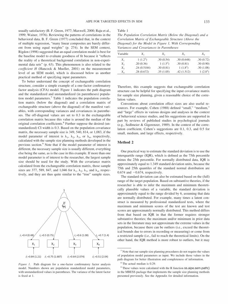
To better understand the concept of exchangeable correlationstructure, consider a simple example of a one-factor confirmatoryfactor analysis (CFA) model. Figure 1 indicates the path diagramand the standardized and unstandardized (in parentheses) popula-tion model parameters.7 Table 1 indicates the population correla-tion matrix (below the diagonal) and a correlation matrix ofexchangeable structure (above the diagonal) of the manifest vari-ables, with corresponding variances and covariances in parenthe-ses. The off-diagonal values are set to 0.3 in the exchangeablecorrelation matrix because this value is around the median of theoriginal correlation coefficients.8 Further suppose the desired (un-standardized) CI width is 0.3. Based on the population covariancematrix, the necessary sample size is 349, 540, 814, or 1,083, if themodel parameter of interest is �1, �2, �3, or �4, respectively,calculated with the sample size planning methods developed in theprevious section.9 Note that if the model parameter of interest isdifferent, the necessary sample size is usually different, everythingelse being the same, as is the case in this example. If more than onemodel parameter is of interest to the researcher, the largest samplesize should be used for the study. With the covariance matrixcalculated from the exchangeable correlation matrix, those samplesizes are 377, 589, 847, and 1,046 for �1, �2, �3, and �4, respec-tively, and they are thus quite similar to the “true” sample sizes.
Therefore, this example suggests that exchangeable correlationstructure can be helpful for specifying the input covariance matrixfor sample size planning, given a reasonable choice of the corre-lation values.
Conventions about correlation effect sizes are also useful re-sources. For example, Cohen (1988) defined “small,” “medium,”and “large” effects in various designs and analyses in the contextof behavioral science studies, and his suggestions are supported inpart by reviews of published studies in psychological journals(e.g., Sedlmeier & Gigerenzer, 1989). In the context of the corre-lation coefficient, Cohen’s suggestions are 0.1, 0.3, and 0.5 forsmall, medium, and large effects, respectively.
Method 2
One practical way to estimate the standard deviation is to use theinterquartile range (IQR), which is defined as the 75th percentileminus the 25th percentile. For normally distributed data, IQR isapproximately equal to 1.349 standard deviation units, because the75th and 25th quantiles of the standard normal distribution are0.674 and �0.674, respectively.
The standard deviation can also be estimated based on the (full)range of the target population. Based on substantive theories, if theresearcher is able to infer the maximum and minimum theoreti-cally plausible values of a variable, the standard deviation isapproximately equal to the range divided by 6, assuming that dataare normally distributed. For example, many times a latent con-struct is measured by professional standardized tests, where themaximum and minimum scores of the test are known and testscores are approximately normally distributed. This method differsfrom that based on IQR in that the former requires strongersubstantive theories; the maximum and/or minimum in prior datasets in the literature may not approximate the extreme values in thepopulation, because there can be outliers (i.e., exceed the theoret-ical bounds due to errors in recording or measuring) or come froma restricted sample (i.e., fail to reach the theoretical limits). On theother hand, the IQR method is more robust to outliers, but it may
7 Note that our sample size planning procedures do not require the valuesof population model parameters as input. We include those values in thepath diagram for better illustration and completeness of information.
8 The actual median is 0.29.9 These values were calculated with the R function ss.aipe.sem.path( )
in the MBESS package that implements the sample size planning methodspresented previously. See the Appendix for detailed information.
λ4 =0.7 (1.4) λ3 =0.6 (1.08) λ2 =0.5 (0.75) λ1 =0.4 (0.48)
1
ξ1
X1 X2 X3 X4
δ1 =0.84 (1.21) δ2 =0.75 (1.687) δ3 =0.64 (2.074) δ4 =0.51 (2.04)
Figure 1. Path diagram for a one-factor confirmatory factor analysismodel. Numbers shown are population standardized model parameters,with unstandardized values in parentheses. The variance of the latent factoris fixed at 1.
Table 1The Population Correlation Matrix (Below the Diagonal) and aCorrelation Matrix of Exchangeable Structure (Above theDiagonal) for the Model in Figure 1, With CorrespondingVariances and Covariances in Parentheses
Variable X1 X2 X3 X4
X1 1 (1.22) .30 (0.54) .30 (0.648) .30 (0.72)X2 .20 (0.36) 1 (1.52) .30 (0.81) .30 (0.90)X3 .24 (0.5184) .30 (0.81) 1 (1.82) .30 (1.08)X4 .28 (0.672) .35 (1.05) .42 (1.512) 1 (2.02)
133AIPE FOR TARGETED EFFECTS IN SEM
rely more heavily on the existence of enough studies that aresimilar to the study in question.
Method 3
In addition to specifying the input covariance matrix directly,one can start from the model parameters (i.e., structural coef-ficients, path loadings, etc.). Based on the model input, if onespecifies the plausible values of the model parameters (i.e.,values in �), the model-implied covariance matrix �(�) can beobtained and can be used as the input �, the covariance matrixof manifest variables. Actually this method is commonly usedin power analysis on the likelihood ratio tests of both the modeloverall fit and model targeted effects (i.e., the method to esti-mate the chi-square noncentrality parameter developed by Sa-torra & Saris, 1985; see also Saris & Satorra, 1993). Hancock(2006) provided a detailed empirical example about how tospecify proper values for model parameters, so as to obtain thepopulation covariance matrix of manifest variables and calcu-late power for SEM.
Obtaining �(�) from � can be accomplished directly with thespecialized R function theta.2.Sigma.theta( ) in the MBESSpackage or indirectly with mainstream SEM software (for anempirical demonstration, see, e.g., Davey & Savla, 2010, Chapter4).10 Generally, it is easier to specify model parameter values inthe standardized metric context, because it is more convenient tohypothesize the magnitude of the relationships in the model interms of standardized coefficients. In particular, the variance of anexogenous variable is always 1, and all sources of variances of anendogenous variable should sum to 1. Therefore, error variancescan be readily obtained after specifying path coefficients. Forexample, suppose the measurement equation of a manifest variableY1 is Y1 � �1�1 � �1, where �1 is the path loading, �1 is anexogenous latent variable, and �1 is the error. In the context ofstandardized metric, suppose, based on prior evidence, the re-searcher estimates the magnitude of �1 to be 0.6, then the errorvariance for Y1 is 0.64 (i.e., 1 � �1
2). Suppose another manifestvariable Y2 has measurement equation Y2 � �2�1 � �3�2 � �2,where �2 and �3 are path loadings, �2 is another exogenous latentvariable, �2 is the error, and the covariance between �1 and �2 is�21. In the standardized metric context, if the researcher estimatesthe magnitude of �2, �3, and �21 to be 0.2, 0.6, and �0.3,respectively, then the error variance of Y2 will be 0.672 (i.e., 1 ��2
2 � �32 � 2�2�3�21). Note that standardized model parameters
imply a correlation matrix rather than a covariance matrix of themanifest variables. After obtaining a correlation matrix, the re-searcher can then apply Methods 1 and 2 discussed above to finallyobtain a covariance matrix.
Method 4
On the measurement level, the reliability coefficient is helpful inestimating path loadings. In practice, many times the latent vari-ables are measured with fully developed tests or scales, and thereliability of those tests are known. Therefore, specifying pathloadings can be largely facilitated by the fact that, in the standard-ized coefficient context, the path loading is the square root of thereliability. This is the case because reliability can be defined as the
variance due to the construct divided by the indicator’s totalvariance, which is 1 in the standardized coefficient context. Forexample, suppose the measurement equation of a manifest variable Y3
is Y3 � �4�3 � �3, using the same notation as previously defined.Further suppose Y3 is a certain standardized test and the reliability ofthis test is known to be 0.9. Because the reliability of this test can bedefined as var(�4�3)/var(�4�3 � �3) (e.g., McDonald, 1999, Chapter7), which is simplified as �4
2 in the standardized metric context, iteasily follows that �4 is approximately 0.949 (i.e., �0.9). A detaileddiscussion of measurement reliability from the factor analytic per-spective is available in McDonald (1999). In fact, such an interpre-tation of reliability is also useful if the researcher specifies modelparameters in the unstandardized coefficient context, in that the errorvariance can still be obtained from the knowledge of the reliabilityand (raw scale) path loading.
Method 5
When the interest lies in the structural coefficients, which isoften the case in studies in the behavioral and social sciences,specification of measurement models can be further simplifiedwith an index called coefficient H, proposed by Hancock andMueller (2001). This index measures the overall quality of afactor’s measurement model; for a given factor with M indicators,it can be defined as
H �
�m�1
M
�m2 /�1 � �m
2 �
1 � �m�1
M
�m2 /�1 � �m
2 �
, (24)
where �m is the standardized path loading of the mth (m � 1, . . . ,M) indicator. Based on Equation 24, H is (a) bounded between 0and 1; (b) unaffected by loadings’ signs; (c) a nondecreasingfunction of M; and (d) larger than or equal to max(�m
2 ), thereliability of the strongest indicator (Hancock & Mueller, 2001).This coefficient can be interpreted as the proportion of variance inthe construct that is explained by its indicators, or the constructreliability associated with each factor’s measurement model. In-terpretations of this index are various (Fornell & Larcker, 1981;Hancock & Mueller, 2001), such as the maximal reliability in thecontext of scale construction (Raykov, 2004). Hancock andKroopnick (2005) demonstrated that the specific value of each pathloading does not affect the overall performance of the SEM modelin terms of the noncentral chi-square distribution of the modelchi-square statistic, as long as different combinations of pathloadings give the same H value. Given the discussion on thecoefficient H and exchangeable correlation structure, therefore, ifthe researcher can anticipate the overall construct reliability (or itsachievable minimum) of a factor’s measurement model, instead ofspecifying the path loading for each indicator, the task can beachieved by using either M indicators whose loadings are all equalto �H/�H � M � MH� or one indicator with loading �H as a
10 See the Appendix for detailed information about the R functiontheta.2.Sigma.theta( ).
134 LAI AND KELLEY
placeholder, although in some situations the latter may implyidentification issues.11 For a detailed empirical example of usingthe coefficient H to specify model parameters in the power analysiscontext, see Hancock (2006, pp. 90–93).
Discussion of Parameter Specification WhenPlanning Sample Size
In summary, we have suggested five practical methods that arehelpful for specifying the input covariance matrix, as a supplementto the literature review, and these methods generally are compat-ible with one another. The researcher can use these methods in amix-and-match manner so that different methods are employedultimately to specify different parts of the input covariance matrix,or can cross-validate the input by comparing the covariance ma-trices specified with different methods.
Any sample size planning method, from either the power-analyticor AIPE perspective, requires educated estimations of populationeffect sizes, and in this regard our methods require no additionalinformation and are no more difficult than others. Actually, poweranalysis for targeted effects in SEM requires the knowledge of allmodel parameters. If a path coefficient in SEM is of interest, one canconduct hypothesis testing on the likelihood ratio of the nested models(i.e., the model with the path estimated and the model with the pathfixed at zero), and infer if the null hypothesis that the path coefficientis zero can be rejected at a certain significance level. Accordingly,sample size planning can be performed so that the likelihood ratio testof the nested models has the desired power. The likelihood ratiofollows a noncentral chi-square distribution, and in order to estimatethe power of the likelihood ratio test, all parameters in the full modeland all parameters in the restricted model are required to calculate thenoncentrality parameter of the distribution (Saris & Satorra, 1993;Satorra & Saris, 1985). Therefore, our sample size planning methodsare no more difficult to implement compared with the commonly usedNHST approach to sample size planning in the literature, because theyrequire a similar amount of input information.
It is also common for any sample size planning procedure that theoutput (i.e., the estimated necessary sample size) depend on thequality of the input parameters. For example, in the context of poweranalysis and sample size planning for SEM, MacCallum, Browne, andCai (2006) acknowledged that the calculated power and sample sizeshould be viewed as approximations, conditional on the input infor-mation and the validity of statistical assumptions (p. 34). It is thenormal state of affairs that sample size planning procedures depend onquantities that are not yet fully known (i.e., population effect sizes),but those procedures can be highly useful in planning and evaluatingresearch design (MacCallum et al., 2006, p. 34). The same reasoningapplies equally to the sample size planning methods in the presentarticle as well.
Specifying the Desired Width
The sample size planning methods presented above require thevalue of the desired CI width in the unstandardized context.Although this value is necessarily context specific and based on thegoals of the study, there is a practical method to facilitate choosingappropriate values for the width. Because it is usually easier toconceptualize the desired CI width in the context of standardized
model coefficients, if the relationship between the unstandardizedand standardized CI widths can be found, the researcher can firstspecify the standardized width and transform it back to the un-standardized scale.
An intuitive but incorrect solution to the present issue is to fit themodel with a correlation matrix: If one puts a correlation matrixinto the covariance structure analysis procedure, the resultingmodel parameter estimates are standardized values, and the CIwidth would thus also be in a standardized metric. Thus it istempting to replace the covariance matrix in the sample sizeplanning methods with a correlation matrix so that one can specifythe desired CI width in terms of standardized values. However,although analyzing a correlation matrix as if it were a covariancematrix generally provides the same point estimates of modelparameters, the standard errors and discrepancy function statisticare incorrect (Cudeck, 1989; Lee, 1985; Shapiro & Browne, 1990).Therefore, the CIs formed based on a correlation matrix are incor-rect. A correct approach to specifying the standardized CI widthmust be based on a covariance matrix.
To find the relationship between unstandardized and standard-ized CI widths, one first needs to understand the relationshipbetween unstandardized and standardized model parameters. Inparticular, a certain standardized path coefficient from a variable Vto a variable U can be defined as (e.g., Bollen, 1989, p. 349)
bUV�s� � bUV
�V
�U� g�bUV�, (25)
where bUV(s) and bUV are the population standardized and unstan-
dardized path coefficients, respectively; �U and �V are the popu-lation standard deviations of variables U and V, respectively; andg(bUV) refers to a function of bUV. If U or V is a manifest variable,�U or �V is directly available from the population covariancematrix of manifest variables; if U or V is a latent variable, itsstandard deviation can be calculated based on population modelparameters. In accordance with the previous discussion on theasymptotic distribution of model parameter estimates, the MLE ofbUV is distributed asymptotically as
�n�bUV � bUV�L¡ N(0, �bUV
2 ), (26)
where �bUV
2 is the corresponding element in the inverse expectedinformation matrix of model parameters as defined in Equation 3.Under the delta method (e.g., Pawitan, 2001, p. 89), the asymptoticdistribution of a function of bUV is
�n� g�bUV� � g�bUV��L¡ N(0, �bUV
2 [g�(bUV)]2), (27)
where g�(bUV) � �V/�U is the first derivative of g( ) evaluated atbUV. Equation 27 can be rewritten as
11 Because all path loadings are equal, Equation 24 reduces to
H �M��2/�1 � �2��
1 � M��2/�1 � �2��,
where � is the path loading. Solving this equation for � gives
� � �H/�H � M � MH�.
135AIPE FOR TARGETED EFFECTS IN SEM
�n�bUV�s� � bUV
�s� �L¡ N0, �bUV
2�V
2
�U2 �, (28)
so that the asymptotic distribution of bUV(s) is derived. Therefore, the
expected CI width for bUV(s) at sample size n is
�s� � 2z1��/ 2
�bUV��V/�U�
�n. (29)
Based on Equation 26, the expected CI width for bUV at samplesize n is
� 2z1��/ 2
�bUV
�n. (30)
Therefore, based on Equations 29 and 30, at the same sample size,the relationship between and (s) can be established:
� �s��U
�V. (31)
Note that although Equation 29 provides a method to calculate thestandardized CI width, itself alone cannot be used to plan for samplesize, because �bUV, �V, and �U are in an unstandardized metric andneed to be necessarily obtained from a covariance matrix.
Given the above discussion of standardized and unstandardized CIwidths, the task of specifying desired CI width can be facilitated withEquation 31. When it is easier to conceptualize the desired CI widthin terms of a standardized metric, the researcher can first determine areasonable value for (s) and then calculate based on Equation 31.Because using a correlation matrix to fit a model generally leads toincorrect solutions, the sample size planning methods in the presentarticle are framed in the context of unstandardized model parametersand always require a covariance matrix as input.
Monte Carlo Simulation Study
Although the distribution of �n converges to multivariate normalas n approaches infinity, at any finite sample size the distributionof �n is only approximately multivariate normal, which impliesthat the sample variance of �j does not exactly follow a chi-squaredistribution. Therefore, it is necessary to ensure the effectivenessof the sample size planning procedures in realistic situations wherethe methods will be applied, especially when the procedure-im-plied sample size is relatively small. If the SEM standard errorestimation theories are exact, the necessary sample size returnedby the sample size planning methods will be exact. Because oursample size planning procedures are necessarily dependent on theMLE, they cannot be expected to work well when maximumlikelihood itself does not work well. Extensive Monte Carlo sim-ulations were conducted to evaluate the performance of the pro-cedures we developed.
The simulation study was conducted in the context of threemodels representative of applied research where SEM is oftenused: (a) a CFA model (Model 1) based on Holzinger and Swin-eford (1939); (b) an autoregressive model (Model 2) based onCurran, Bollen, Chen, Paxton, and Kirby (2003) and Paxton,Curran, Bollen, Kirby, and Chen (2001); and (c) a complex SEM
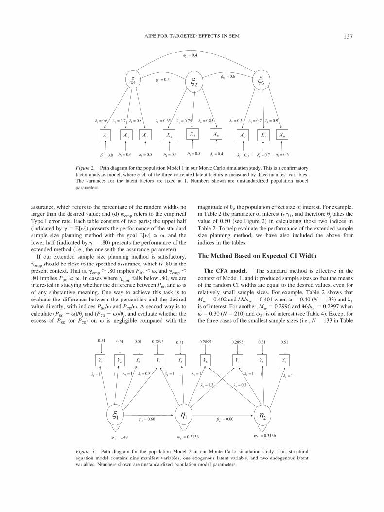
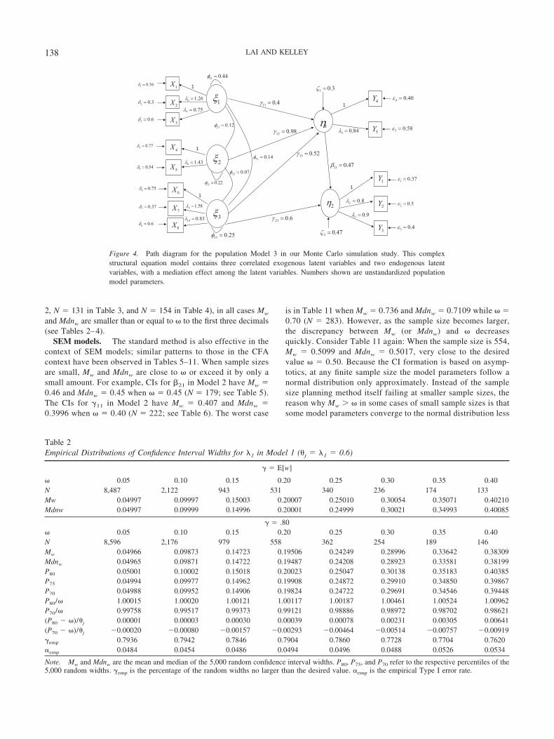
model (Model 3) with mediation among latent variables, based onMaruyama and McGarvey (1980). Some modifications of theoriginal model and/or parameters were made so that these modelsare more generally applicable. Path diagrams and model parame-ters used in the Monte Carlo simulation are provided in Figures2–4.
Given the models, we first specified the unstandardized modelparameters, whose values are indicated in Figures 2–4. Afterspecifying the model and model parameters, the model-impliedpopulation covariance matrix, �(�), can be obtained, and it is usedas the population covariance matrix of the manifest variables, thatis, � � �(�). The specifications of the present simulation studyshould not be confused with the input of our sample size planningmethods, which do not include the model parameters. The speci-fied model parameters of interest include factor loadings (e.g., �1
in Model 1, �6 in Model 2), structural path coefficients (e.g., �21
in Model 2, �11 in Model 3), and covariances between latentvariables (e.g., �21 in Model 1). The targeted effects are meant torepresent a variety and magnitude of possible effects in an SEMcontext. We planned the sample size with regard to the expected CIwidth (i.e., with the goal that E[w] � ), as well as with the goalto achieve assurance of .80 (i.e., the extended method with � set to.80). The value of .80 is reasonable for our simulation studybecause (a) the CI observed in a study is ensured to be sufficientlynarrow with relatively high assurance; (b) not all the randomwidths are narrower than desired, so that the sample size returnedby the planning procedure can be ascertained to be the minimumnecessary. This is the case because if � is set to a very large value(e.g., .99) and all the random widths are narrower than desired, itis unknown whether it is because the planning procedure gave acorrect sample size, or because a larger than necessary (i.e., notcorrect) sample size was used. Given (a) the particular model, (b)the population covariance matrix �, (c) the model parameter ofinterest �j, and (d) the desired width , the necessary sample sizeN is returned from the sample size planning procedures (N � n asdefined in Equation 13, or N � n� as defined in Equation 22). Arandom sample of size N was generated from a multivariate normaldistribution with the MASS package (Venables & Ripley, 2002) inR with the population covariance being equal to �.12 Then we fitthe model with the sample covariance matrix using maximumlikelihood and calculated the standard error of �j using the sempackage (Fox, 2006) in R. A 95% CI for �j was formed. Eachcondition was replicated 5,000 times. There is no guideline regard-ing the appropriate number of replications, and currently the typ-ical number in the SEM context is 1,000. Generally, the larger thenumber is, the more reliable the simulation results are, other thingsbeing the same. We used 5,000 replications so that the results aremore reliable than if each condition was repeated 1,000 times.
Results
Simulation results are reported in detail in Tables 2–11, where(a) the mean (Mw) and median (Mdnw) of the 5,000 random CIwidths are given; (b) P80, P75, and P70 refer to the subscriptedpercentiles of the 5,000 random widths; (c) �emp is the empirical
12 MASS was originally an acronym for Modern Applied Statistics withS, but is used as a stand-alone package title now.
136 LAI AND KELLEY
assurance, which refers to the percentage of the random widths nolarger than the desired value; and (d) �emp refers to the empiricalType I error rate. Each table consists of two parts; the upper half(indicated by � � E[w]) presents the performance of the standardsample size planning method with the goal E[w] � , and thelower half (indicated by � � .80) presents the performance of theextended method (i.e., the one with the assurance parameter).
If our extended sample size planning method is satisfactory,�emp should be close to the specified assurance, which is .80 in thepresent context. That is, �emp � .80 implies P80 � , and �emp �.80 implies P80 � . In cases where �emp falls below .80, we areinterested in studying whether the difference between P80 and isof any substantive meaning. One way to achieve this task is toevaluate the difference between the percentiles and the desiredvalue directly, with indices P80/ and P70/ . A second way is tocalculate (P80 � )/�j and (P70 � )/�j, and evaluate whether theexcess of P80 (or P70) on is negligible compared with the
magnitude of �j, the population effect size of interest. For example,in Table 2 the parameter of interest is �1, and therefore �j takes thevalue of 0.60 (see Figure 2) in calculating those two indices inTable 2. To help evaluate the performance of the extended samplesize planning method, we have also included the above fourindices in the tables.
The Method Based on Expected CI Width
The CFA model. The standard method is effective in thecontext of Model 1, and it produced sample sizes so that the meansof the random CI widths are equal to the desired values, even forrelatively small sample sizes. For example, Table 2 shows thatMw � 0.402 and Mdnw � 0.401 when � 0.40 (N � 133) and �1
is of interest. For another, Mw � 0.2996 and Mdnw � 0.2997 when � 0.30 (N � 210) and �21 is of interest (see Table 4). Except forthe three cases of the smallest sample sizes (i.e., N � 133 in Table
32 0.6
31 0.4
6 0.855 0.754 0.653 0.82 0.71 0.6 7 0.5 8 0.7 9 0.9
1 2 3
1X 2X 3X 4X 5X 6X7X 8X 9X
1 0.8 2 0.6 3 0.5 4 0.6 5 0.5 6 0.47 0.7 8 0.7 9 0.6
21 0.5
Figure 2. Path diagram for the population Model 1 in our Monte Carlo simulation study. This is a confirmatoryfactor analysis model, where each of the three correlated latent factors is measured by three manifest variables.The variances for the latent factors are fixed at 1. Numbers shown are unstandardized population modelparameters.
1 1 1 2 1 3 0.3 4 1 1 5 1
6 0.3 7 0.3
8 19 11
11 0.49 11 0.3136 22 0.3136
11 0.60 21 0.60
0.51
211
1Y 2Y 3Y 4Y 5Y 6Y 7Y 9Y8Y
0.51 0.51 0.2895 0.51 0.2895 0.2895 0.51 0.51
Figure 3. Path diagram for the population Model 2 in our Monte Carlo simulation study. This structuralequation model contains nine manifest variables, one exogenous latent variable, and two endogenous latentvariables. Numbers shown are unstandardized population model parameters.
137AIPE FOR TARGETED EFFECTS IN SEM
2, N � 131 in Table 3, and N � 154 in Table 4), in all cases Mw
and Mdnw are smaller than or equal to to the first three decimals(see Tables 2–4).
SEM models. The standard method is also effective in thecontext of SEM models; similar patterns to those in the CFAcontext have been observed in Tables 5–11. When sample sizesare small, Mw and Mdnw are close to or exceed it by only asmall amount. For example, CIs for �21 in Model 2 have Mw �0.46 and Mdnw � 0.45 when � 0.45 (N � 179; see Table 5).The CIs for �11 in Model 2 have Mw � 0.407 and Mdnw �0.3996 when � 0.40 (N � 222; see Table 6). The worst case
is in Table 11 when Mw � 0.736 and Mdnw � 0.7109 while �0.70 (N � 283). However, as the sample size becomes larger,the discrepancy between Mw (or Mdnw) and decreasesquickly. Consider Table 11 again: When the sample size is 554,Mw � 0.5099 and Mdnw � 0.5017, very close to the desiredvalue � 0.50. Because the CI formation is based on asymp-totics, at any finite sample size the model parameters follow anormal distribution only approximately. Instead of the samplesize planning method itself failing at smaller sample sizes, thereason why Mw � in some cases of small sample sizes is thatsome model parameters converge to the normal distribution less
1 0.56
6 1.26
7 0.75
8 1.48 1.43
9 1.58
10 0.83
21 0.12
13 0.52
11 0.4
1 0.37
2 0.5
3 0.423 0.6
11 0.44
22 0.22
33 0.25
31 0.14
32 0.07
4 0.40
5 0.58
21 0.47
1 0.3
2 0.47
12 0.98 5 0.84
2 0.8
3 0.93
2
1
1X
2X
3X
2 0.3
3 0.6
5X
4X4 0.77
5 0.54
6X6 0.75
7X7 0.37
8X8 0.6
1
2
1Y
2Y
3Y
4Y
5Y
Figure 4. Path diagram for the population Model 3 in our Monte Carlo simulation study. This complexstructural equation model contains three correlated exogenous latent variables and two endogenous latentvariables, with a mediation effect among the latent variables. Numbers shown are unstandardized populationmodel parameters.
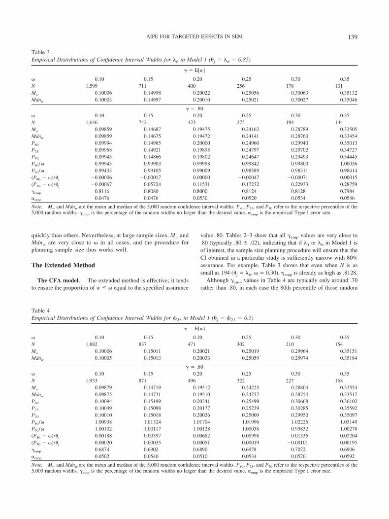
Table 2Empirical Distributions of Confidence Interval Widths for �1 in Model 1 (�j � �1 � 0.6)
� � E[w]
0.05 0.10 0.15 0.20 0.25 0.30 0.35 0.40N 8,487 2,122 943 531 340 236 174 133Mw 0.04997 0.09997 0.15003 0.20007 0.25010 0.30054 0.35071 0.40210Mdnw 0.04997 0.09999 0.14996 0.20001 0.24999 0.30021 0.34993 0.40085
� � .80 0.05 0.10 0.15 0.20 0.25 0.30 0.35 0.40N 8,596 2,176 979 558 362 254 189 146Mw 0.04966 0.09873 0.14723 0.19506 0.24249 0.28996 0.33642 0.38309Mdnw 0.04965 0.09871 0.14722 0.19487 0.24208 0.28923 0.33581 0.38199P80 0.05001 0.10002 0.15018 0.20023 0.25047 0.30138 0.35183 0.40385P75 0.04994 0.09977 0.14962 0.19908 0.24872 0.29910 0.34850 0.39867P70 0.04988 0.09952 0.14906 0.19824 0.24722 0.29691 0.34546 0.39448P80/ 1.00015 1.00020 1.00121 1.00117 1.00187 1.00461 1.00524 1.00962P70/ 0.99758 0.99517 0.99373 0.99121 0.98886 0.98972 0.98702 0.98621(P80 � )/�j 0.00001 0.00003 0.00030 0.00039 0.00078 0.00231 0.00305 0.00641(P70 � )/�j �0.00020 �0.00080 �0.00157 �0.00293 �0.00464 �0.00514 �0.00757 �0.00919�emp 0.7936 0.7942 0.7846 0.7904 0.7860 0.7728 0.7704 0.7620�emp 0.0484 0.0454 0.0486 0.0494 0.0496 0.0488 0.0526 0.0534
Note. Mw and Mdnw are the mean and median of the 5,000 random confidence interval widths. P80, P75, and P70 refer to the respective percentiles of the5,000 random widths. �emp is the percentage of the random widths no larger than the desired value. �emp is the empirical Type I error rate.
138 LAI AND KELLEY
quickly than others. Nevertheless, at large sample sizes, Mw andMdnw are very close to in all cases, and the procedure forplanning sample size thus works well.
The Extended Method
The CFA model. The extended method is effective; it tendsto ensure the proportion of w � equal to the specified assurance
value .80. Tables 2–3 show that all �emp values are very close to.80 (typically .80 � .02), indicating that if �1 or �6 in Model 1 isof interest, the sample size planning procedure will ensure that theCI obtained in a particular study is sufficiently narrow with 80%assurance. For example, Table 3 shows that even when N is assmall as 194 (�j � �6, � 0.30), �emp is already as high as .8128.
Although �emp values in Table 4 are typically only around .70rather than .80, in each case the 80th percentile of those random
Table 3Empirical Distributions of Confidence Interval Widths for �6 in Model 1 (�j � �6 � 0.85)
� � E[w]
0.10 0.15 0.20 0.25 0.30 0.35N 1,599 711 400 256 178 131Mw 0.10006 0.14998 0.20022 0.25056 0.30063 0.35132Mdnw 0.10003 0.14997 0.20010 0.25021 0.30027 0.35046
� � .80 0.10 0.15 0.20 0.25 0.30 0.35N 1,646 742 423 275 194 144Mw 0.09859 0.14687 0.19475 0.24162 0.28789 0.33505Mdnw 0.09859 0.14675 0.19472 0.24141 0.28760 0.33454P80 0.09994 0.14985 0.20000 0.24960 0.29940 0.35013P75 0.09968 0.14921 0.19895 0.24797 0.29702 0.34727P70 0.09943 0.14866 0.19802 0.24647 0.29493 0.34445P80/ 0.99943 0.99903 0.99998 0.99842 0.99800 1.00036P70/ 0.99433 0.99105 0.99009 0.98589 0.98311 0.98414(P80 � )/�j �0.00006 �0.00017 0.00000 �0.00047 �0.00071 0.00015(P70 � )/�j �0.00067 0.05724 0.11531 0.17232 0.22933 0.28759�emp 0.8116 0.8080 0.8000 0.8124 0.8128 0.7984�emp 0.0476 0.0476 0.0530 0.0520 0.0534 0.0546
Note. Mw and Mdnw are the mean and median of the 5,000 random confidence interval widths. P80, P75, and P70 refer to the respective percentiles of the5,000 random widths. �emp is the percentage of the random widths no larger than the desired value. �emp is the empirical Type I error rate.
Table 4Empirical Distributions of Confidence Interval Widths for �21 in Model 1 (�j � �21 � 0.5)
� � E[w]
0.10 0.15 0.20 0.25 0.30 0.35N 1,882 837 471 302 210 154Mw 0.10006 0.15011 0.20021 0.25019 0.29964 0.35151Mdnw 0.10005 0.15013 0.20033 0.25059 0.29974 0.35184
� � .80 0.10 0.15 0.20 0.25 0.30 0.35N 1,933 871 496 322 227 168Mw 0.09879 0.14719 0.19512 0.24225 0.28804 0.33554Mdnw 0.09875 0.14731 0.19510 0.24237 0.28754 0.33517P80 0.10094 0.15199 0.20341 0.25499 0.30668 0.36102P75 0.10049 0.15098 0.20177 0.25239 0.30285 0.35592P70 0.10010 0.15018 0.20026 0.25009 0.29950 0.35097P80/ 1.00938 1.01324 1.01704 1.01996 1.02226 1.03149P70/ 1.00102 1.00117 1.00128 1.00038 0.99832 1.00278(P80 � )/�j 0.00188 0.00397 0.00682 0.00998 0.01336 0.02204(P70 � )/�j 0.00020 0.00035 0.00051 0.00019 �0.00101 0.00195�emp 0.6874 0.6902 0.6890 0.6978 0.7072 0.6906�emp 0.0502 0.0540 0.0510 0.0534 0.0570 0.0592
Note. Mw and Mdnw are the mean and median of the 5,000 random confidence interval widths. P80, P75, and P70 refer to the respective percentiles of the5,000 random widths. �emp is the percentage of the random widths no larger than the desired value. �emp is the empirical Type I error rate.
139AIPE FOR TARGETED EFFECTS IN SEM
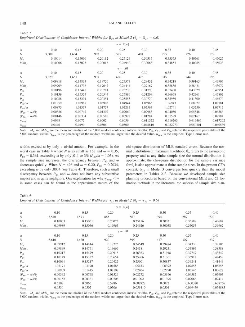
widths exceed by only a trivial amount. For example, in theworst case in Table 4 where N is as small as 168 and � 0.35,P80 � 0.361, exceeding by only .011 or 3% (P80/ � 1.03). Asthe sample size increases, the discrepancy between P80 and decreases quickly: When N � 496 and � 0.20, P80 � 0.2034,exceeding by only .0034 (see Table 4). Therefore, such a smalldiscrepancy between P80 and does not have any substantiveimpact and is quite negligible. One explanation for why �emp � �in some cases can be found in the approximate nature of the
chi-square distribution of MLE standard errors. Because the nor-mal distribution of maximum likelihood �n refers to the asymptoticproperty and at any finite sample size the normal distribution isapproximate, the chi-square distribution for the sample variancefor �j is also approximate at finite sample sizes. In the present CFAcontext, �21 in Model 3 converges less quickly than the modelparameters in Tables 2–3. Because we developed sample sizeplanning procedures based on the conventional MLE and CI for-mation methods in the literature, the success of sample size plan-
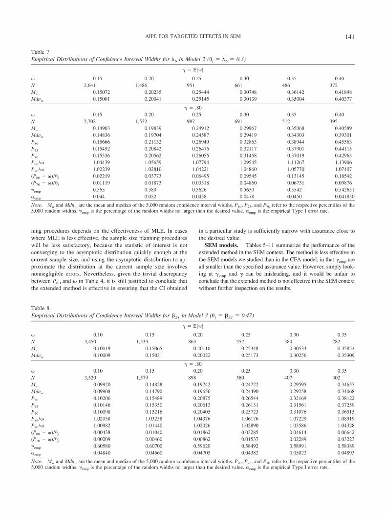
Table 5Empirical Distributions of Confidence Interval Widths for �21 in Model 2 (�j � �21 � 0.6)
� � E[w]
0.10 0.15 0.20 0.25 0.30 0.35 0.40 0.45N 3,608 1,604 902 578 401 295 226 179Mw 0.10014 0.15060 0.20112 0.25124 0.30315 0.35355 0.40761 0.46027Mdnw 0.10006 0.15023 0.20016 0.24942 0.30068 0.34853 0.40085 0.45023
� � .80 0.10 0.15 0.20 0.25 0.30 0.35 0.40 0.45N 3,679 1,651 937 606 425 315 244 195Mw 0.09918 0.14833 0.19720 0.24577 0.29452 0.34218 0.39163 0.43905Mdnw 0.09909 0.14796 0.19647 0.24444 0.29169 0.33836 0.38431 0.43079P80 0.10196 0.15445 0.20781 0.26236 0.31790 0.37430 0.43329 0.48951P75 0.10139 0.15324 0.20544 0.25880 0.31209 0.36668 0.42361 0.47802P70 0.10088 0.15201 0.20351 0.25553 0.30770 0.35959 0.41300 0.46670P80/ 1.01959 1.02968 1.03905 1.04944 1.05965 1.06943 1.08322 1.08781P70/ 1.00875 1.01337 1.01757 1.02213 1.02567 1.02741 1.03250 1.03712(P80 � )/�j 0.00326 0.00742 0.01302 0.02060 0.02983 0.04050 0.05548 0.06586(P70 � )/�j 0.00146 0.00334 0.00586 0.00922 0.01284 0.01599 0.02167 0.02784�emp 0.6098 0.6072 0.6002 0.6036 0.611522 0.616263 0.616466 0.617202�emp 0.0446 0.0490 0.0506 0.0500 0.048810 0.052273 0.050201 0.060569
Note. Mw and Mdnw are the mean and median of the 5,000 random confidence interval widths. P80, P75, and P70 refer to the respective percentiles of the5,000 random widths. �emp is the percentage of the random widths no larger than the desired value. �emp is the empirical Type I error rate.
Table 6Empirical Distributions of Confidence Interval Widths for �11 in Model 2 (�j � �11 � 0.6)
� � E[w]
0.10 0.15 0.20 0.25 0.30 0.35 0.40N 3,540 1,573 885 567 394 289 222M
w0.10003 0.15061 0.20073 0.25116 0.30321 0.35588 0.40684
Mdnw 0.09989 0.15036 0.19965 0.24926 0.30038 0.35053 0.39962
� � .80 0.10 0.15 0.20 0.25 0.30 0.35 0.40N 3,610 1,620 920 595 417 309 239Mw 0.09912 0.14814 0.19725 0.24549 0.29474 0.34330 0.39106Mdnw 0.09899 0.14771 0.19666 0.24381 0.29231 0.33895 0.38388P80 0.10217 0.15479 0.20918 0.26363 0.31918 0.37749 0.43542P75 0.10149 0.15337 0.20654 0.25966 0.31361 0.36912 0.42459P70 0.10091 0.15217 0.20422 0.25601 0.30837 0.36241 0.41449P80/ 1.02171 1.03190 1.04588 1.05453 1.06392 1.07855 1.08855P70/ 1.00909 1.01445 1.02108 1.02404 1.02790 1.03545 1.03622(P80 � )/�j 0.00362 0.00798 0.01529 0.02272 0.03196 0.04582 0.05903(P70 � )/�j 0.00152 0.00361 0.00703 0.01002 0.01395 0.02068 0.02414�emp 0.6108 0.6066 0.5986 0.608922 0.6072 0.600320 0.608766�emp 0.0530 0.0502 0.0506 0.051410 0.0504 0.049459 0.054885
Note. Mw and Mdnw are the mean and median of the 5,000 random confidence interval widths. P80, P75, and P70 refer to the respective percentiles of the5,000 random widths. �emp is the percentage of the random widths no larger than the desired value. �emp is the empirical Type I error rate.
140 LAI AND KELLEY
ning procedures depends on the effectiveness of MLE. In caseswhere MLE is less effective, the sample size planning procedureswill be less satisfactory, because the statistic of interest is notconverging to the asymptotic distribution quickly enough at thecurrent sample size, and using the asymptotic distribution to ap-proximate the distribution at the current sample size involvesnonnegligible errors. Nevertheless, given the trivial discrepancybetween P80 and in Table 4, it is still justified to conclude thatthe extended method is effective in ensuring that the CI obtained
in a particular study is sufficiently narrow with assurance close tothe desired value.
SEM models. Tables 5–11 summarize the performance of theextended method in the SEM context. The method is less effective inthe SEM models we studied than in the CFA model, in that �emp areall smaller than the specified assurance value. However, simply look-ing at �emp and � can be misleading, and it would be unfair toconclude that the extended method is not effective in the SEM contextwithout further inspection on the results.
Table 7Empirical Distributions of Confidence Interval Widths for �6 in Model 2 (�j � �6 � 0.3)
� � E[w]
0.15 0.20 0.25 0.30 0.35 0.40N 2,641 1,486 951 661 486 372Mw 0.15072 0.20235 0.25444 0.30748 0.36142 0.41898Mdnw 0.15001 0.20041 0.25145 0.30139 0.35004 0.40377
� � .80 0.15 0.20 0.25 0.30 0.35 0.40N 2,702 1,532 987 691 512 395Mw 0.14903 0.19839 0.24912 0.29967 0.35068 0.40589Mdnw 0.14836 0.19704 0.24587 0.29419 0.34303 0.39301P80 0.15666 0.21132 0.26949 0.32863 0.38944 0.45563P75 0.15492 0.20842 0.26476 0.32117 0.37901 0.44115P70 0.15336 0.20562 0.26055 0.31458 0.37019 0.42963P80/ 1.04439 1.05659 1.07794 1.09545 1.11267 1.13906P70/ 1.02239 1.02810 1.04221 1.04860 1.05770 1.07407(P80 � )/�j 0.02219 0.03773 0.06495 0.09545 0.13145 0.18542(P70 � )/�j 0.01119 0.01873 0.03518 0.04860 0.06731 0.09876�emp 0.565 0.580 0.5626 0.5650 0.5542 0.542651�emp 0.044 0.052 0.0458 0.0478 0.0450 0.041850
Note. Mw and Mdnw are the mean and median of the 5,000 random confidence interval widths. P80, P75, and P70 refer to the respective percentiles of the5,000 random widths. �emp is the percentage of the random widths no larger than the desired value. �emp is the empirical Type I error rate.
Table 8Empirical Distributions of Confidence Interval Widths for �21 in Model 3 (�j � �21 � 0.47)
� � E[w]
0.10 0.15 0.20 0.25 0.30 0.35N 3,450 1,533 863 552 384 282Mw 0.10019 0.15065 0.20110 0.25348 0.30533 0.35853Mdnw 0.10009 0.15031 0.20022 0.25173 0.30256 0.35309
� � .80 0.10 0.15 0.20 0.25 0.30 0.35N 3,520 1,579 898 580 407 302Mw 0.09920 0.14828 0.19742 0.24722 0.29595 0.34657Mdnw 0.09908 0.14790 0.19656 0.24490 0.29258 0.34068P80 0.10206 0.15489 0.20875 0.26544 0.32169 0.38122P75 0.10146 0.15350 0.20613 0.26131 0.31561 0.37259P70 0.10098 0.15216 0.20405 0.25723 0.31076 0.36515P80/ 1.02058 1.03258 1.04376 1.06176 1.07229 1.08919P70/ 1.00982 1.01440 1.02026 1.02890 1.03586 1.04328(P80 � )/�j 0.00438 0.01040 0.01862 0.03285 0.04614 0.06642(P70 � )/�j 0.00209 0.00460 0.00862 0.01537 0.02289 0.03223�emp 0.60580 0.60700 0.59620 0.58492 0.58991 0.58389�emp 0.04840 0.04660 0.04705 0.04382 0.05022 0.04893
Note. Mw and Mdnw are the mean and median of the 5,000 random confidence interval widths. P80, P75, and P70 refer to the respective percentiles of the5,000 random widths. �emp is the percentage of the random widths no larger than the desired value. �emp is the empirical Type I error rate.
141AIPE FOR TARGETED EFFECTS IN SEM
In most cases, at smaller sample sizes, the 80th percentiles of therandom widths exceed the desired value by only a negligibleamount. For example, P80 in Table 5 is 0.374 when � 0.35 (N �315) and 0.318 when � 0.30 (N � 425); the differences are only.024 and .018, respectively. Similar patterns are observed in mostof the situations, such as Table 6, where P80 � 0.377 and � 0.35when N � 309; Table 8, where P80 � 0.322 and � 0.30 whenN � 407; and Table 10, where P80 � 0.107 and � 0.10 whenN � 570.
There are some situations where the results at smaller samplesizes are less satisfactory. For example, when the desired width is0.40, P80 � 0.456 (N � 395; see Table 7), exceeding by almost14%. However, in this case the empirical Type I error rate is only.042, less than the nominal rate .05. Instead of forming intervals atthe 95% confidence level, the MLE generally gives 96% CIs in thissituation, which are wider than 95% ones. Therefore, at least partof the reason for the random CI widths being wider than by anontrivial amount is because the MLE is not yet effective enough
Table 9Empirical Distributions of Confidence Interval Widths for �10 in Model 3 (�j � �10 � 0.83)
� � E[w]
0.15 0.20 0.25 0.30 0.35 0.40 0.45N 4,435 2,495 1,597 1,109 815 624 493Mw 0.15041 0.20081 0.25190 0.30307 0.35532 0.40627 0.46136Mdnw 0.15019 0.19989 0.25012 0.30004 0.35099 0.39921 0.45079
� � .80 0.15 0.20 0.25 0.30 0.35 0.40 0.45N 4,514 2,554 1,644 1,148 849 653 519Mw 0.14896 0.19858 0.24802 0.29761 0.34744 0.39713 0.44877Mdnw 0.14857 0.19769 0.24692 0.29490 0.34261 0.39026 0.43861P80 0.15532 0.20983 0.26570 0.32255 0.38076 0.43934 0.50546P75 0.15389 0.20741 0.26164 0.31671 0.37314 0.42934 0.49074P70 0.15273 0.20508 0.25839 0.31160 0.36619 0.42022 0.47791P80/ 1.03548 1.04917 1.06278 1.07517 1.08788 1.09834 1.12325P70/ 1.01823 1.02538 1.03356 1.03865 1.04627 1.05056 1.06203(P80 � )/�j 0.00641 0.01185 0.01891 0.02717 0.03706 0.04739 0.06682(P70 � )/�j 0.00329 0.00612 0.01011 0.01397 0.01951 0.02437 0.03363�emp 0.56720 0.56960 0.55760 0.56514 0.56814 0.56842 0.56464�emp 0.05280 0.04920 0.05520 0.05283 0.04990 0.04896 0.04692
Note. Mw and Mdnw are the mean and median of the 5,000 random confidence interval widths. P80, P75, and P70 refer to the respective percentiles of the5,000 random widths. �emp is the percentage of the random widths no larger than the desired value. �emp is the empirical Type I error rate.
Table 10Empirical Distributions of Confidence Interval Widths for �31 in Model 3 (�j � �31 � 0.14)
� � E[w]
0.03 0.04 0.05 0.06 0.07 0.08 0.09 0.10N 6,025 3,389 2,169 1,507 1,107 848 670 543Mw 0.02999 0.04000 0.05011 0.06016 0.06999 0.08003 0.09017 0.10020Mdnw 0.02998 0.04000 0.05009 0.06010 0.06989 0.07993 0.08992 0.10009
� � .80 0.03 0.04 0.05 0.06 0.07 0.08 0.09 0.10N 6,117 3,458 2,224 1,553 1,146 882 700 570Mw 0.02977 0.03959 0.04939 0.05917 0.06880 0.07864 0.08816 0.09772Mdnw 0.02979 0.03958 0.04934 0.05915 0.06873 0.07858 0.08817 0.09745P80 0.03056 0.04099 0.05167 0.06230 0.07310 0.08400 0.09523 0.10658P75 0.03040 0.04073 0.05124 0.06165 0.07225 0.08292 0.09371 0.10476P70 0.03027 0.04049 0.05082 0.06111 0.07146 0.08188 0.09239 0.10326P80/ 1.01859 1.02484 1.03343 1.03840 1.04435 1.05000 1.05806 1.06583P70/ 1.00911 1.01236 1.01644 1.01842 1.02086 1.02348 1.02654 1.03257(P80 � )/�j 0.00398 0.00710 0.01194 0.01646 0.02218 0.02857 0.03733 0.04702(P70 � )/�j 0.00195 0.00353 0.00587 0.00790 0.01043 0.01341 0.01706 0.02326�emp 0.5912 0.6016 0.5940 0.5860 0.5930 0.5890 0.5850 0.5970�emp 0.0448 0.0528 0.0546 0.0542 0.0528 0.0509 0.0564 0.0605
Note. Mw and Mdnw are the mean and median of the 5,000 random confidence interval widths. P80, P75, and P70 refer to the respective percentiles of the5,000 random widths. �emp is the percentage of the random widths no larger than the desired value. �emp is the empirical Type I error rate.
142 LAI AND KELLEY
at the current sample size and gives larger standard error estimatesthan it should. Similar patterns can be found in Tables 9 and 11,where for smaller sample sizes P80 exceeds by a nontrivialamount (e.g., P80/ � 1.10). Nevertheless, in these cases (i.e.,Tables 7, 9, and 11) the 70th percentiles exceed by only anegligible amount. Consider N � 395 and � 0.40 in Table 7again. In this case P70 � 0.4296, exceeding by .0296, or about7%, and the discrepancy can be considered as trivial. For another,Table 9 shows that P70 � 0.4779 when N � 519, and exceeds �0.45 by .0279, or about 6%. Given the above comparisons of the70th and 80th quantiles to the desired width value, it can be seenthat at smaller sample sizes where MLE is not effective enoughand overestimates the standard errors, the extended method tendsto underestimate the necessary sample. Within the simulationstudy in the present article, in worst cases the sample size returnedby the extended method ensures that a CI obtained is sufficientlynarrow about 70% of the time when the desired assurance is set to.80.
When the sample size is relatively large, in all cases the extendedprocedure returns the necessary sample sizes such that a CI obtainedis sufficiently narrow with close to 80% assurance. Although �emp
values for the SEM models are less than the specified value .80 in allcases, the 80th quantiles of those random CI widths are very close tothe corresponding desired values, and the discrepancy between thetwo does not have substantive impact. For example, P80 � 0.1022 inTable 6 when N � 3,610 and � 0.10, exceeding by 2.1%; P80 �0.102 in Table 8 when N � 3,520 and � 0.10, exceeding by 2%;P80 � 0.154 in Table 11 when N � 6,240 and � 0.15, exceeding by 2.9%.
In summary, the extensive Monte Carlo simulation study indicatesthat both the standard and extended sample size planning proceduresare effective in estimating the necessary sample size according to thespecified goals. The standard method is quite effective in both theCFA and SEM contexts, and the sample size returned indeed ensures
that the expected CI width is no wider than desired. The extendedmethod is most effective in the CFA context, and in most of the casesthe empirical proportion of sufficiently narrow random CIs is close tothe specified .80 level. Although in the SEM context, the extendedmethod tends to underestimate the necessary sample size in caseswhere MLE is less effective, the 80th percentile of the random CIwidths usually exceeds the desired width by only a negligible amountthat has no substantive impact, and the discrepancy between the 80thpercentile and decreases as the sample size increases.
Issues in Statistical Theory
We discuss two issues regarding the assumptions of our samplesize planning methods: (a) the model is correctly specified, and (b)data are normally distributed. Neither of these two assumptions isunique to our sample size planning methods; in fact, these assump-tions are commonly made not only in sample size planning but in theSEM literature as a whole. For example, the power analysis onlikelihood ratio tests of nested models is based on the assumption thatthe full model (i.e., the one with the path coefficients of interestestimated) is correctly specified (see, e.g., Hancock, 2006; Saris &Sattora, 1993; Satorra & Saris, 1985). In addition, the asymptoticchi-square distribution of the model chi-square statistic is based on theassumption that data follow a multivariate normal distribution (see,e.g., MacCallum et al., 2006; Steiger, Shapiro, & Browne, 1985). Asdiscussed below, the implications of the violations of these twoassumptions are still open to study.
Model Misspecifications
The methods developed in the present article are based on theassumption that the model is correctly specified, but in practice itmay be difficult to develop an exactly correct model. However,
Table 11Empirical Distributions of Confidence Interval Widths for �23 in Model 3 (�j � �23 � 0.6)
� � E[w]
0.15 0.20 0.25 0.30 0.40 0.50 0.60 0.70N 6,147 3,458 2,213 1,537 865 554 385 283Mw 0.15036 0.20088 0.25107 0.30225 0.40638 0.50994 0.62067 0.73600Mdnw 0.15000 0.20027 0.24993 0.30033 0.40173 0.50165 0.60517 0.71091
� � .80 0.15 0.20 0.25 0.30 0.40 0.50 0.60 0.70N 6,240 3,528 2,269 1,583 900 582 408 303Mw 0.14921 0.19897 0.24831 0.29806 0.39759 0.49956 0.60272 0.71296Mdnw 0.14896 0.19833 0.24748 0.29665 0.39311 0.49074 0.58775 0.68600P80 0.15437 0.20783 0.26228 0.31774 0.43254 0.55298 0.67729 0.81377P75 0.15326 0.20589 0.25916 0.31350 0.42426 0.54004 0.65950 0.78712P70 0.15234 0.20415 0.25631 0.30973 0.41788 0.52951 0.64174 0.76097P80/ 1.02914 1.03913 1.04914 1.05912 1.08136 1.10595 1.12882 1.16253P70/ 1.01560 1.02075 1.02524 1.03244 1.04470 1.05901 1.06957 1.08710(P80 � )/�j 0.00728 0.01304 0.02047 0.02956 0.05424 0.08829 0.12882 0.18962(P70 � )/�j 0.00390 0.00692 0.01052 0.01622 0.02980 0.04918 0.06957 0.10162�emp 0.5610 0.5620 0.5580 0.5530 0.5620 0.5520 0.5490 0.5440�emp 0.0528 0.0468 0.0518 0.0426 0.0487 0.0442 0.0510 0.0461
Note. Mw and Mdnw are the mean and median of the 5,000 random confidence interval widths. P80, P75, and P70 refer to the respective percentiles of the5,000 random widths. �emp is the percentage of the random widths no larger than the desired value. �emp is the empirical Type I error rate.
143AIPE FOR TARGETED EFFECTS IN SEM
sample size planning can proceed as long as the proposed model isreasonable (i.e., close to the true model), under the additionalassumption called population drift (or parameter drift), which inessence states that the proposed model is not badly misspecifiedand that lack of fit due to model misspecification is approximatelyof the same magnitude as lack of fit due to sampling error (Steigeret al., 1985; see also MacCallum et al., 2006). Actually thepopulation drift assumption was used to derive the asymptoticchi-square distribution of the chi-square model fit statistic inSteiger et al. (1985), and thus is commonly recognized as areasonable assumption in the SEM literature. For a more formalstatement and discussion of this assumption, see Steiger et al.(1985; see also Browne & Cudeck, 1992; MacCallum et al., 2006).
Nevertheless, it is not clear when a “badly specified” model isbad enough, and in practice it is generally not possible to verify thepopulation drift assumption. The issue of how misspecifications ofmodels influence the empirical distribution of CI width and samplesize planning methods is open to study, but it is not the focus of thepresent article. The effects of misspecifications of a model can bestudied empirically with a priori Monte Carlo simulations in amanner similar to that discussed in Muthen and Muthen (2002) andPaxton et al. (2001). A random sample is generated based on thetrue model-implied covariance matrix, whereas the sample size isplanned based on the proposed model (i.e., on the [incorrect]assumption that � � �(�)). Various properties of the random CIwidth can be studied based on a large number of replications offitting the proposed model to the random data. Specialized Rfunctions have been included in the MBESS package to implementsuch an a priori Monte Carlo simulation study, so that researcherscan try with different models and study the effects of the inputmodel on the returned sample size when planning the samplesize.13
Nonnormal Distributions
It is still an issue open to study in the literature regarding theeffects of nonnormal data on estimating various effect sizes inSEM (e.g., model fit indices, targeted effects), especially in thesample size planning stage, although some solutions to analyzenonnormal data have been developed (e.g., Browne, 1984; Kano,Berkane, & Bentler, 1990; Yuan & Bentler, 1997, 1998a, 1998b;Yuan, Bentler, & Zhang 2005; Yuan, Chan, & Bentler, 2000; Yuan& Hayashi, 2006). Generally, robust methods give larger standarderror estimations than do standard methods (e.g., the Wald CI wereviewed in a previous section), which implies that the CI returnedby robust methods tend to be wider than those returned by standardmethods, other things being the same. Thus one should note that ifthe researcher plans the sample size based on our methods and usesrobust methods to analyze the data, the CI obtained might not besufficiently narrow, if the normality assumption is seriously vio-lated. Nevertheless, we do recommend using robust methods toanalyze data, because in reality the normality assumption is usuallyviolated to different extents. We based our sample size planningmethods on the normality assumption mainly because (a) robustmethods, both analytical treatments and bootstrap applications,require raw data, which are unavailable in the research design stage;(b) the problem of nonnormal data can be alleviated by better or morecareful data collecting methods and/or data transformation; and (c) inorder to study the behavior of the CI width obtained in a study, which
is a random variable dependent on � and the covariance matrix of �,both of which are also random variables, certain assumptions must bemade regarding the distribution of the data.
Discussion
When a researcher designs a study, there are at least three waysto decide the sample size: (a) collect as many participants asresources allow, (b) follow rules of thumb, or (c) apply formalsample size planning methods that attempt to accomplish a spec-ified goal. Recruiting fewer participants than necessary can be awaste of resources because the study fails to achieve its goals.Using more than necessary participants is also a waste of resourcesin the sense that the extra data do not necessarily increase theunderstanding of the topic under study. Rules of thumb in the SEMliterature are usually based on simulation studies. Those simula-tions were conducted in different contexts, and conclusions drawnregarding the “appropriate” sample size are based on variouscriteria. However, MacCallum, Widaman, Zhang, and Hong(1999), in the CFA context, demonstrated that rules of thumb aregenerally invalid because the performance of estimation is highlydependent on the model characteristics. Given that SEM is morecomplex than CFA, the rules of thumb should perform no better inSEM. In fact, by reviewing recent psychological studies that applySEM, MacCallum and Austin (2000) recommended against theuse of rules of thumb. The only reasonable option left is formalsample size planning methods. The necessary sample size can beplanned with rigorously derived statistical methods so that thedesired goals can be accomplished. Although sample size planningmethods are based on assumptions that tend not to hold perfectlyin reality, they are based on rigorous statistical reasoning andshould perform reasonably well in most cases, as long as theassumptions are not seriously violated. Thus, the option of formalsample size planning methods is preferred.
The sample size for an SEM study can be planned from at leastthe power-analytic perspective or the AIPE perspective. Whentargeted effects in SEM are of interest, often of interest are notonly their directions but their magnitude. The dichotomous resultobtained by NHST (i.e., if the population effect is larger than zeroor smaller than zero, without loss of generality) does not neces-sarily answer the question about the population effect size. On theother hand, a CI provides a range of plausible values for thepopulation parameter of interest and thus helps better understandthe magnitude of the population effect. With the goal of obtainingnarrow CIs for the targeted effects of interest in SEM, sample sizeplanning methods are developed from the AIPE perspective.
Sample size planning methods from AIPE require educated esti-mation of the population effect sizes, as does the power perspective(for power analysis in SEM, see, e.g., Hancock, 2006; Hancock &Freeman, 2001; Kim, 2005; MacCallum et al., 2006; MacCallum,Browne, & Sugawara, 1996; Satorra & Saris, 1985; for power anal-ysis in general, see also Cohen, 1988; Murphy & Myors, 2004). Thetask of specifying the input effect sizes needs to be accomplished byconsulting the literature. It is natural in the course of the accumulation
13 This simulation study can be performed with the specialized R func-tion ss.aipe.sem.path.sensitiv( ) in MBESS. See the Appendix for de-tailed information.
144 LAI AND KELLEY
of knowledge that the specification of some not fully known infor-mation as input needs to be finished before conducting the investiga-tion: Ongoing research updates the current knowledge based on earlylooks at the data from previous studies (Coffey & Muller, 2003;Proschan, 2005). In fact, Senn (2002) pointed out:
This is common to all science. An astronomer does not know themagnitude of new stars until he has found them, but the magnitude ofstar he is looking for determines how much he has to spend on atelescope. (p. 1304)
In the spirit of the increasing urge that applied studies reporteffect sizes and CIs, we believe that sample size planning from theAIPE perspective should be considered when targeted effects areof interest in an SEM context. If an SEM model parameter ofinterest has a wide CI, its value is unclear. Thus a narrow CI isdesirable because it excludes more implausible values and furtherpins down the population parameter. We believe the AIPE ap-proach to planning sample sizes for SEM studies when targetedeffects are of interest will help to better understand the magnitudeof the effects in the population and evaluate substantive theories.
References
American Educational Research Association. (2006). Standards for report-ing on empirical social science research in AERA publications. Educa-tional Researcher, 35, 33–40. doi:10.3102/0013189X035006033
American Psychological Association. (2001). Publication manual of theAmerican Psychological Association (5th ed.). Washington, DC: Au-thor.
American Psychological Association. (2010). Publication manual of theAmerican Psychological Association (6th ed.). Washington, DC: Amer-ican Psychological Association.
Anderson, T. W. (2003). An introduction to multivariate statistical analysis(3rd ed.). New York, NY: Wiley.
Arminger, G., & Schoenberg, R. J. (1989). Pseudo maximum likelihoodestimation and a test for misspecification in mean and covariancestructure models. Psychometrika, 54, 409 – 425. doi:10.1007/BF02294626
Bentler, P. M., & Bonett, D. G. (1980). Significance tests and goodness-of-fit in the analysis of covariance structures. Psychological Bulletin, 88,588–606. doi:10.1037/0033-2909.88.3.588
Bentler, P. M., & Dudgeon, P. (1996). Covariance structure analysis:Statistical practice, theory, directions. Annual Review of Psychology, 47,563–592. doi:10.1146/annurev.psych.47.1.563
Beran, R., & Srivastava, M. S. (1985). Bootstrap tests and confidenceregions for functions of a covariance matrix. Annuals of Statistics, 13,95–115. doi:10.1214/aos/1176346579
Bollen, K. A. (1989). Structural equations with latent variables. NewYork, NY: Wiley.
Bollen, K. A. (2002). Latent variables in psychology and the social sci-ences. Annual Review of Psychology, 53, 605–634. doi:10.1146/annurev.psych.53.100901.135239
Bollen, K. A., & Stine, R. (1993). Bootstrapping goodness-of-fit measuresin structural equation models. In K. A. Bollen & J. S. Long (Eds.),Testing structural equation models (pp. 111–135). Newbury Park, CA:Sage.
Browne, M. W. (1984). Asymptotic distribution-free methods for theanalysis of covariance structures. British Journal of Mathematical andStatistical Psychology, 37, 62–83.
Browne, M. W., & Arminger, G. (1995). Specification and estimation ofmean- and covariance-structure models. In G. Arminger, C. C. Clogg, &
M. E. Sobel (Eds.), Handbook of statistical modeling for the social andbehavioral sciences (pp. 185–249). New York, NY: Plenum.
Browne, M. W., & Cudeck, R. (1992). Alternative ways of assessing modelfit. Sociological Methods & Research, 21, 230–258. doi:10.1177/0049124192021002005
Casella, G., & Berger, R. L. (2002). Statistical inference (2nd ed.). Bel-mont, CA: Duxbury Press.
Coffey, C. S., & Muller, K. E. (2003). Properties of internal pilots with theunivariate approach to repeated measures. Statistics in Medicine, 22,2469–2485. doi:10.1002/sim.1466
Cohen, J. (1988). Statistical power analysis for the behavioral sciences(2nd ed.). Hillsdale, NJ: Erlbaum.
Cohen, J. (1994). The earth is round (p � .05). American Psychologist, 49,997–1003. doi:10.1037/0003-066X.49.12.997
Cudeck, R. (1989). Analysis of correlation matrices using covariancestructure models. Psychological Bulletin, 105, 317–327. doi:10.1037/0033-2909.105.2.317
Curran, P. J., Bollen, K. A., Chen, F., Paxton, P., & Kirby, J. B. (2003).Finite sampling properties of the point estimates and confidence inter-vals of the RMSEA. Sociological Methods & Research, 32, 208–252.doi:10.1177/0049124103256130
Curran-Everett, D., & Benos, D. J. (2004). Guidelines for reporting statis-tics in journals published by the American Physiological Society. Jour-nal of Neurophysiology, 92, 669–671. doi:10.1152/jn.00534.2004
Davey, A., & Savla, J. (2010). Statistical power analysis with missing data:A structural equation modeling approach. New York, NY: Taylor &Francis.
Efron, B., & Tibshirani, R. J. (1993). An introduction to the bootstrap. NewYork, NY: Chapman & Hall/CRC.
Fornell, C., & Larcker, D. F. (1981). Evaluating structural equation modelswith unobservable variables and measurement error. Journal of Mar-keting Research, 18, 39–50. doi:10.2307/3151312
Fox, J. (2006). Structural equation modeling with the sem packagein R. Structural Equation Modeling, 13, 465– 486. doi:10.1207/s15328007sem1303_7
Green, B. F. (1977). Parameter sensitivity in multivariate methods.Multivariate Behavioral Research, 12, 263–287. doi:10.1207/s15327906mbr1203_1
Green, S. B. (1991). How many subjects does it take to do a regressionanalysis? Multivariate Behavioral Research, 26, 499–510. doi:10.1207/s15327906mbr2603_7
Guenther, W. C. (1965). Concepts of statistical inference. New York, NY:McGraw-Hill.
Hancock, G. R. (2006). Power analysis in covariance structure modeling.In G. R. Hancock & R. O. Mueller (Eds.), Structural equation modeling:A second course (pp. 69–115). Greenwich, CT: Information Age.
Hancock, G. R., & Freeman, M. J. (2001). Power and sample size for theroot mean square error of approximation test of not close fit in structuralequation modeling. Educational and Psychological Measurement, 61,741–758. doi:10.1177/00131640121971491
Hancock, G. R., & Kroopnick, M. H. (2005, April). A simplified samplesize determination for tests of latent covariance structure parameters.Paper presented at the annual meeting of the American EducationalResearch Association, Montreal, Canada.
Hancock, G. R., & Mueller, R. O. (2001). Rethinking construct reliabilitywithin latent variable systems. In R. Cudeck, S. H. C. du Toit, & D.Sörbom (Eds.), Structural equation modeling: Past and present. AFestschrift in honor of Karl G. Jöreskog (pp. 195–216). Chicago, IL:Scientific Software International.
Harlow, L. L., Mulaik, S. A., & Steiger, J. H. (Eds.). (1997). What if therewere no significance tests? Mahwah, NJ: Erlbaum.
Holzinger, K. J., & Swineford, F. (1939). A study in factor analysis: Thestability of a bi-factor solution. Chicago, IL: University of Chicago.
International Committee of Medical Journal Editors. (2004). Uniform
145AIPE FOR TARGETED EFFECTS IN SEM
requirements for manuscripts submitted to biomedical journals: Writingand editing for biomedical publication. Philadelphia, PA: Author.
Kano, Y., Berkane, M., & Bentler, P. M. (1990). Covariance structureanalysis with heterogeneous kurtosis parameters. Biometrika, 77, 575–585. doi:10.1093/biomet/77.3.575
Kelley, K. (2007a). Confidence intervals for standardized effect sizes:Theory, application, and implementation. Journal of Statistical Soft-ware, 20, 1–24.
Kelley, K. (2007b). Methods for the behavioral, educational, and socialsciences: An R package. Behavior Research Methods, 39, 979–984.
Kelley, K. (2007c). Sample size planning for the coefficient of variationfrom the accuracy in parameter estimation approach. Behavior ResearchMethods, 39, 755–766.
Kelley, K. (2008). Sample size planning for the squared multiple correla-tion coefficient: Accuracy in parameter estimation via narrow confi-dence intervals. Multivariate Behavioral Research, 43, 524–555. doi:10.1080/00273170802490632
Kelley, K., & Lai, K. (2010). MBESS [Computer software manual]. Re-trieved from http://www.cran.r-project.org
Kelley, K., & Maxwell, S. E. (2003). Sample size for multiple regression:Obtaining regression coefficients that are accurate, not simply signifi-cant. Psychological Methods, 8, 305–321. doi:10.1037/1082-989X.8.3.305
Kelley, K., Maxwell, S. E., & Rausch, J. R. (2003). Obtaining poweror obtaining precision: Delineating methods of sample-size planning.Evaluation and the Health Professions, 26, 258–287. doi:10.1177/0163278703255242
Kelley, K., & Rausch, J. R. (2006). Sample size planning for the standard-ized mean difference: Accuracy in parameter estimation via narrowconfidence intervals. Psychological Methods, 11, 363–385. doi:10.1037/1082-989X.11.4.363
Kim, K. H. (2005). The relation among fit indexes, power, and sample sizein structural equation modeling. Structural Equation Modeling, 12,368–390. doi:10.1207/s15328007sem1203_2
Lee, S.-Y. (1985). Analysis of covariance and correlation structures. Com-putational Statistics & Data Analysis, 2, 279–295. doi:10.1016/0167-9473(85)90002-7
Lehmann, E. L. (1998). Elements of large-sample theory. New York, NY:Springer.
MacCallum, R. C., & Austin, J. T. (2000). Applications of structuralequation modeling in psychological research. Annual Review of Psy-chology, 51, 201–226. doi:10.1146/annurev.psych.51.1.201
MacCallum, R. C., Browne, M. W., & Cai, L. (2006). Testing differencesbetween nested covariance structure models: Power analysis and nullhypotheses. Psychological Methods, 11, 19–35. doi:10.1037/1082-989X.11.1.19
MacCallum, R. C., Browne, M. W., & Sugawara, H. M. (1996). Poweranalysis and determination of sample size for covariance structuremodeling. Psychological Methods, 1, 130–149. doi:10.1037/1082-989X.1.2.130
MacCallum, R. C., Widaman, K. F., Zhang, S., & Hong, S. (1999). Samplesize in factor analysis. Psychological Methods, 4, 84–99. doi:10.1037/1082-989X.4.1.84
Mace, A. E. (1964). Sample-size determination. New York, NY: Reinhold.Maruyama, G., & McGarvey, B. (1980). Evaluating causal models: An
application of maximum-likelihood analysis of structural equations.Psychological Bulletin, 87, 502–512. doi:10.1037/0033-2909.87.3.502
Maxwell, S. E. (2000). Sample size and multiple regression analysis.Psychological Methods, 5, 434–458. doi:10.1037/1082-989X.5.4.434
Maxwell, S. E., Kelley, K., & Rausch, J. R. (2008). Sample size planningfor statistical power and accuracy in parameter estimation. AnnualReview of Psychology, 59, 537–563. doi:10.1146/annurev.psych.59.103006.093735
McArdle, J. J., & McDonald, R. P. (1984). Some algebraic properties of the
reticular action model for moment structures. British Journal of Math-ematical and Statistical Psychology, 37, 234–251.
McDonald, R. P. (1999). Test theory: A unified treatment. Mahwah, NJ:Erlbaum.
Meehl, P. E. (1997). The problem in epistemology, not statistics: Replacingsignificance tests by confidence intervals and quantify accuracy of riskynumerical predictions. In L. L. Harlow, S. A. Mulaik, & J. H. Steiger(Eds.), What if there were no significance tests? (pp. 393–426). Mah-wah, NJ: Erlbaum.
Mulaik, S. A. (2009). Linear causal modeling with structural equations.Boca Raton, FL: Chapman & Hall.
Murphy, K. R., & Myors, B. (2004). Statistical power analysis: A simpleand general model for traditional and modern hypothesis tests (2nd ed.).Mahwah, NJ: Erlbaum.
Muthen, L. K., & Muthen, B. O. (2002). How to use a Monte Carlo studyto decide on sample size and determine power. Structural EquationModeling, 9, 599–620. doi:10.1207/S15328007SEM0904_8
Nickerson, R. S. (2000). Null hypothesis significance testing: A review ofan old and continuing controversy. Psychological Methods, 5, 241–301.doi:10.1037/1082-989X.5.2.241
Pawitan, Y. (2001). In all likelihood: Statistical modelling and inferenceusing likelihood. New York, NY: Oxford University Press.
Paxton, P., Curran, P. J., Bollen, K. A., Kirby, J., & Chen, F. (2001). MonteCarlo experiments: Design and implementation. Structural EquationModeling, 8, 287–312. doi:10.1207/S15328007SEM0802_7
Proschan, M. A. (2005). Two-stage sample size re-estimation based on anuisance parameter: A review. Journal of Biopharmaceutical Statistics,15, 559–574. doi:10.1081/BIP-200062852
Raju, N. S., Bilgic, R., Edwards, J. E., & Fleer, P. F. (1999). Accuracy ofpopulation validity and cross-validity estimation: An empirical compar-ison of formula-based, traditional empirical, and equal weights proce-dures. Applied Psychological Measurement, 23, 99–115. doi:10.1177/01466219922031220
Raykov, T. (2004). Estimation of maximal reliability: A note on a cova-riance structure modelling approach. British Journal of Mathematicaland Statistical Psychology, 57, 21–27. doi:10.1348/000711004849295
R Development Core Team. (2010). R: A language and environment forstatistical computing [Computer software manual]. Vienna, Austria: RFoundation for Statistical Computing.
Rigdon, E. E. (1998). The equal correlation baseline model for comparativefit assessment in structural equation modeling. Structural EquationModeling, 5, 63–77. doi:10.1080/10705519809540089
Saris, W. E., & Satorra, A. (1993). Power evaluations in structural equationmodels. In K. A. Bollen & J. S. Long (Eds.), Testing structural equationmodels (pp. 181–204). Newbury Park, CA: Sage.
Satorra, A., & Saris, W. E. (1985). The power of the likelihood ratio testin covariance structure analysis. Psychometrika, 50, 83–90. doi:10.1007/BF02294150
Schmidt, F. L. (1996). Statistical significance testing and cumulativeknowledge in psychology: Implications for training of researchers. Psy-chological Methods, 1, 115–129. doi:10.1037/1082-989X.1.2.115
Sedlmeier, P., & Gigerenzer, G. (1989). Do studies of statistical powerhave an effect on the power of studies? Psychological Bulletin, 105,309–316. doi:10.1037/0033-2909.105.2.309
Senn, S. J. (2002). Power is indeed irrelevant in interpreting completed studies.British Medical Journal, 325, 1304. doi:10.1136/bmj.325.7375.1304
Shapiro, A. (1983). Asymptotic distribution theory in the analysis of covariancestructures (a unified approach). South African Statistical Journal, 17, 33–81.
Shapiro, A., & Browne, M. W. (1990). On the treatment of correlationstructures as covariance structures. Linear Algebra and Its Applications,127, 567–587. doi:10.1016/0024-3795(90)90362-G
Steiger, J. H., & Lind, J. C. (1980, May). Statistically-based tests for thenumber of common factors. Paper presented at the annual meeting of thePsychometric Society, Iowa City, IA.
146 LAI AND KELLEY
Steiger, J. H., Shapiro, A., & Browne, M. W. (1985). On the multivariateasymptotic distribution of sequential chi-square statistics. Psy-chometrika, 50, 253–263. doi:10.1007/BF02294104
Venables, W. N., & Ripley, B. D. (2002). Modern applied statistics with S(4th ed.). New York, NY: Springer.
Wainer, H. (1976). Estimating coefficients in linear models: It don’t make nonevermind. Psychological Bulletin, 83, 213–217. doi:10.1037/0033-2909.83.2.213
White, H. (1982). Maximum likelihood estimation of misspecified models.Econometrica, 50, 1–25. doi:10.2307/1912526
Yuan, K.-H., & Bentler, P. M. (1997). Improving parameter tests incovariance structure analysis. Computational Statistics & Data Analysis,26, 177–198. doi:10.1016/S0167-9473(97)00025-X
Yuan, K.-H., & Bentler, P. M. (1998a). Robust mean and covariancestructure analysis. British Journal of Mathematical and Statistical Psy-chology, 51, 63–88.
Yuan, K.-H., & Bentler, P. M. (1998b). Structural equation modeling withrobust covariances. Sociological Methodology, 28, 363–396. doi:10.1111/0081-1750.00052
Yuan, K.-H., Bentler, P. M., & Zhang, W. (2005). The effect of skewnessand kurtosis on mean and covariance structure analysis: The univariatecase and its multivariate implication. Sociological Methods & Research,34, 240–258. doi:10.1177/0049124105280200
Yuan, K.-H., Chan, W., & Bentler, P. M. (2000). Robust transformationwith applications to structural equation modelling. British Journal ofMathematical and Statistical Psychology, 53, 31–50. doi:10.1348/000711000159169
Yuan, K.-H., & Hayashi, K. (2006). Standard errors in covariancestructure models: Asymptotics versus bootstrap. British Journal ofMathematical and Statistical Psychology, 59, 397– 417. doi:10.1348/000711005X85896
Appendix
Implementing the Methods Discussed With MBESS
All the methods discussed in the present article have beenimplemented in R functions (R Development Core Team, 2010) inthe MBESS package (Kelley, 2007a, 2007c; Kelley & Lai, 2010).This appendix briefly discusses how to use those functions to planfor sample size; more detailed documentation is available in thehelp files in the MBESS package. Functions in the appendix callthe sem package (Fox, 2006) in R when they need to fit structuralequation models (SEMs). Models are specified in the RAM nota-tion (see, e.g., McArdle & McDonald, 1984) in the same manneras the sem R package, which uses a one-headed arrow to representthe regression effect and a two-headed arrow to represent thevariance or covariance. A successfully specified model objectshould be of class “mod” in R. Readers interested in how to specifymodels in R using the RAM notation are referred to Fox (2006) orthe help files of the sem and MBESS packages. This appendix alsoincludes a brief example about SEM model specifications in theRAM notation.
To plan for sample size, the user first needs to specify the model,which can be performed with the function specify.model() in thesem package. For example, to specify the one-factor confirmatoryfactor analysis (CFA) model in Figure 1, the following syntax canbe used:
� library(MBESS)� library(sem)
� model.cfa �- specify.model()xi1 -� X1, lam1, 0.5xi1 -� X2, lam2, 0.5xi1 -� X3, lam3, 0.5xi1 -� X4, lam4, 0.5xi1 �-� xi1, NA, 1X1 �-� X1, del1, 0.5X2 �-� X2, del2, 0.5X3 �-� X3, del3, 0.5X4 �-� X4, del4, 0.5
In each line of the model specification above, there are threeparts, separated by commas. The first part indicates the path, thesecond part indicates the name of this particular path coefficient,and the third part indicates the starting value for this path coeffi-cient in estimation. If the path name is NA, then the path is fixedat the value in the third part. For example, the variance of xi1 inthis model is fixed at 1.
The function theta.2.Sigma.theta() in MBESS creates themodel-implied covariance matrix given a model and model param-eter values. This function is not used in sample size planning butis convenient for constructing a covariance matrix as input forsample size planning or conducting simulation studies. For exam-ple, given the population standardized model parameters in Figure1, the model-implied correlation matrix can be obtained as follows:
(Appendix continues)
147AIPE FOR TARGETED EFFECTS IN SEM
� theta.cfa �- c(.4, .5, .6, .7, .84, .75, .64, .51)� names(theta.cfa) �- c(“lam1”, “lam2”, “lam3”, “lam4”,
“del1”, “del2”, “del3”, “del4”)� res �- theta.2.Sigma.theta(model�model.cfa, theta�
theta.cfa, latent.vars�“xi1”)� cor.mat �- res$Sigma.theta
The argument model is an object of “mod” class containing thespecifications of an SEM model, theta is a vector of modelparameters, and latent.vars is a vector indicating the names of thelatent variables in the model.
The function ss.aipe.sem.path() plans for sample size forSEM with the goal of obtaining a sufficiently narrow confidenceinterval (CI) for a model parameter of interest. Suppose �1 in theabove one-factor CFA model is of interest, and it is desired tohave a confidence interval for �1 no wider than 0.3. To replicatethe example that we used to illustrate the concept of exchangeablecorrelation structure in the text, we specify the standard deviationsof X1, X2, X3, and X4 to be 1.2, 1.5, 1.8, and 2, respectively. Thenthe following syntax can be used to calculate the necessary samplesize:
� SD �- diag(c(1.2, 1.5, 1.8, 2))� rownames(SD)�-colnames(SD)�- c(“X1”,“X2”,“X3”,“X4”)� Sigma.cfa �- SD %*% cor.mat %*% SD� ss.aipe.sem.path(model�model.cfa, Sigma�Sigma.cfa,
desired.width�0.3, which.path�“lam1”)
The sample size returned is 349. The argument Sigma refers to theinput covariance matrix of the manifest variables, desired.width
refers to the desired CI width, and which.path is name of the modelparameter of interest. If one desires to have .80 assurance that the CIobtained will be no wider than desired, the argument assurance canbe added to the function:
� ss.aipe.sem.path(model�model.cfa, Sigma�Sigma.cfa,desired.width�0.3, which.path�“lam1”, assurance�.80)
The function ss.aipe.sem.path.sensitiv() can be used to con-duct a priori Monte Carlo simulations to study how misspecifica-tions of model and/or the covariance matrix of manifest variablesaffect the effectiveness of sample size planning methods. Anexample call to this function is
� ss.aipe.sem.path.sensitiv(model, est.Sigma, true.Sigma�est.Sigma, which.path, desired.width, G�1000),
where random data are generated based on the true covariancematrix of manifest variables (true.Sigma) but fit to the proposedmodel (model), whereas the sample size is planned based on theproposed model and the estimated covariance matrix of manifestvariables (est.Sigma). Various properties of the random CIwidths can be studied empirically by replicating the process a largenumber of times (i.e., the argument G).
Received May 14, 2009Revision received September 2, 2010
Accepted September 7, 2010 �
Showcase your work in APA’s newest database.
Make your tests available to other researchers and students; get wider recognition for your work.
“PsycTESTS is going to be an outstanding resource for psychology,” said Ronald F. Levant, PhD. “I was among the first to provide some of my tests and was happy to do so. They will be available for others to use—and will relieve me of the administrative tasks of providing them to individuals.”
Visit http://www.apa.org/pubs/databases/psyctests/call-for-tests.aspx to learn more about PsycTESTS and how you can participate.
Questions? Call 1-800-374-2722 or write to [email protected] since PsycARTICLES has a database been so eagerly anticipated!
148 LAI AND KELLEY


![ProstateMRI,withorwithoutMRI-targetedbiopsy,and ... · 2019. 5. 4. · [Diagnostic Test Accuracy Review] Prostate MRI, with or without MRI-targeted biopsy, and systematic biopsy for](https://img.pdfslide.net/doc/110x75/614907fc9241b00fbd674bbd/prostatemriwithorwithoutmri-targetedbiopsyand-2019-5-4-diagnostic-test.jpg)


![ProstateMRI,withorwithoutMRI-targetedbiopsy,and ...doccdn.simplesite.com/d/a7/85/281756459332109735/8... · [Diagnostic Test Accuracy Review] Prostate MRI, with or without MRI-targeted](https://img.pdfslide.net/doc/110x75/5e67d4d211dfb66b806b9099/prostatemriwithorwithoutmri-targetedbiopsyand-diagnostic-test-accuracy-review.jpg)