Embed Size (px)
Citation preview

Accuracy, Precision and Efficiency in Sparse Grids
John Burkardt,Information Technology Department,
Virginia Tech...........
http://people.sc.fsu.edu/∼jburkardt/presentations/ajou 2009 sparse.pdf
..........Mathematics Department,
Ajou University,Suwon, Korea,08 May 2009.
Burkardt Accuracy, Precision and Efficiency in Sparse Grids
Accuracy, Precision and Efficiency in Sparse Grids
1 Introduction
2 Quadrature Rules in 1D
3 Product Rules for Higher Dimensions
4 Smolyak Quadrature
5 Covering Pascal’s Triangle
6 How Grids Combine
7 Sparse Grids in Action
8 Smoothness is Necessary
9 A Stochastic Diffusion Equation
10 Conclusion
Burkardt Accuracy, Precision and Efficiency in Sparse Grids
INTRODUCTION: Accuracy, Precision, Efficiency
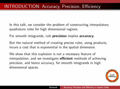
In this talk, we consider the problem of constructing interpolatoryquadrature rules for high dimensional regions.
For smooth integrands, rule precision implies accuracy.
But the natural method of creating precise rules, using products,incurs a cost that is exponential in the spatial dimension.
We show that this explosion is not a necessary feature ofinterpolation, and we investigate efficient methods of achievingprecision, and hence accuracy, for smooth integrands in highdimensional spaces.
Burkardt Accuracy, Precision and Efficiency in Sparse Grids
Accuracy, Precision and Efficiency in Sparse Grids
1 Introduction
2 Quadrature Rules in 1D
3 Product Rules for Higher Dimensions
4 Smolyak Quadrature
5 Covering Pascal’s Triangle
6 How Grids Combine
7 Sparse Grids in Action
8 Smoothness is Necessary
9 A Stochastic Diffusion Equation
10 Conclusion
Burkardt Accuracy, Precision and Efficiency in Sparse Grids
QUADRATURE: Approximation of Integrals
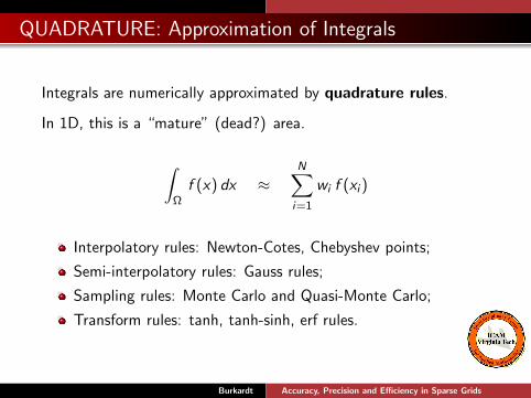
Integrals are numerically approximated by quadrature rules.
In 1D, this is a “mature” (dead?) area.
∫Ω
f (x) dx ≈N∑i=1
wi f (xi )
Interpolatory rules: Newton-Cotes, Chebyshev points;
Semi-interpolatory rules: Gauss rules;
Sampling rules: Monte Carlo and Quasi-Monte Carlo;
Transform rules: tanh, tanh-sinh, erf rules.
Burkardt Accuracy, Precision and Efficiency in Sparse Grids

QUADRATURE: Families of Rules
Most quadrature rules are available in any order N.
Generally, increasing N produces a more accurate result(more about this in a minute!)
Under that assumption, a cautious calculation uses a sequence ofincreasing values of N.
An efficient calculation chooses the sequence of N in such a waythat previous function values can be reused. This is called nesting.
Burkardt Accuracy, Precision and Efficiency in Sparse Grids
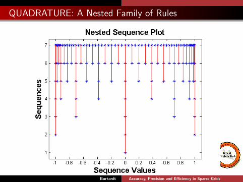
QUADRATURE: A Nested Family of Rules
Burkardt Accuracy, Precision and Efficiency in Sparse Grids
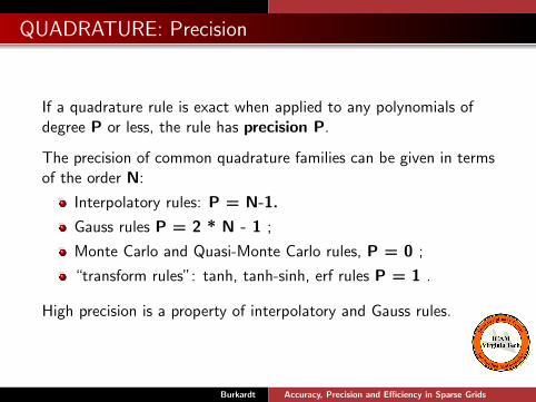
QUADRATURE: Precision
If a quadrature rule is exact when applied to any polynomials ofdegree P or less, the rule has precision P.
The precision of common quadrature families can be given in termsof the order N:
Interpolatory rules: P = N-1.
Gauss rules P = 2 * N - 1 ;
Monte Carlo and Quasi-Monte Carlo rules, P = 0 ;
“transform rules”: tanh, tanh-sinh, erf rules P = 1 .
High precision is a property of interpolatory and Gauss rules.
Burkardt Accuracy, Precision and Efficiency in Sparse Grids
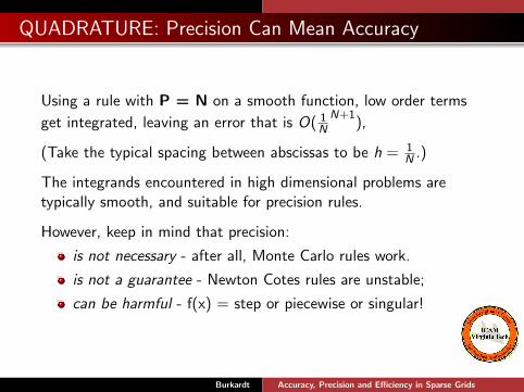
QUADRATURE: Precision Can Mean Accuracy
Using a rule with P = N on a smooth function, low order terms
get integrated, leaving an error that is O( 1N
N+1),
(Take the typical spacing between abscissas to be h = 1N .)
The integrands encountered in high dimensional problems aretypically smooth, and suitable for precision rules.
However, keep in mind that precision:
is not necessary - after all, Monte Carlo rules work.
is not a guarantee - Newton Cotes rules are unstable;
can be harmful - f(x) = step or piecewise or singular!
Burkardt Accuracy, Precision and Efficiency in Sparse Grids
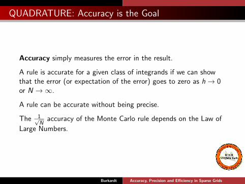
QUADRATURE: Accuracy is the Goal
Accuracy simply measures the error in the result.
A rule is accurate for a given class of integrands if we can showthat the error (or expectation of the error) goes to zero as h→ 0or N →∞.
A rule can be accurate without being precise.
The 1√N
accuracy of the Monte Carlo rule depends on the Law of
Large Numbers.
Burkardt Accuracy, Precision and Efficiency in Sparse Grids

QUADRATURE: Efficiency is the Number of Abscissas
Efficiency measures the amount of work expended for the result.
For quadrature, we measure our work in terms of the number offunction evaluations, which in turn is the number of abscissas.
Since it is common to use a sequence of rules, it is important, forefficiency, to take advantage of nestedness, that is, to choose afamily of rule for which the function values at one level can bereused on the next.
Burkardt Accuracy, Precision and Efficiency in Sparse Grids
Accuracy, Precision and Efficiency in Sparse Grids
1 Introduction
2 Quadrature Rules in 1D
3 Product Rules for Higher Dimensions
4 Smolyak Quadrature
5 Covering Pascal’s Triangle
6 How Grids Combine
7 Sparse Grids in Action
8 Smoothness is Necessary
9 A Stochastic Diffusion Equation
10 Conclusion
Burkardt Accuracy, Precision and Efficiency in Sparse Grids
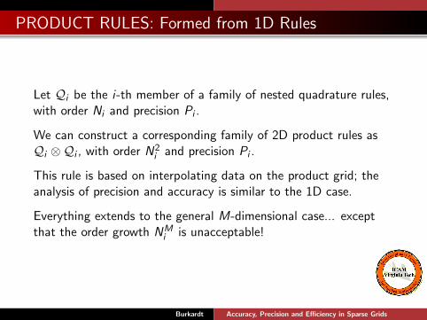
PRODUCT RULES: Formed from 1D Rules
Let Qi be the i-th member of a family of nested quadrature rules,with order Ni and precision Pi .
We can construct a corresponding family of 2D product rules asQi ⊗Qi , with order N2
i and precision Pi .
This rule is based on interpolating data on the product grid; theanalysis of precision and accuracy is similar to the 1D case.
Everything extends to the general M-dimensional case... exceptthat the order growth NM
i is unacceptable!
Burkardt Accuracy, Precision and Efficiency in Sparse Grids
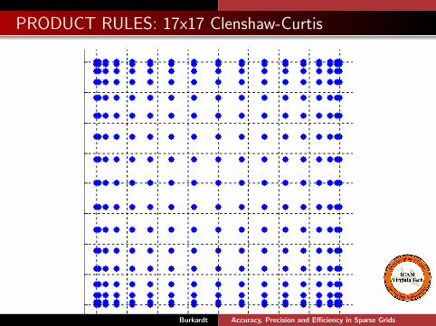
PRODUCT RULES: 17x17 Clenshaw-Curtis
Burkardt Accuracy, Precision and Efficiency in Sparse Grids

PRODUCT RULES: Do We Get Our Money’s Worth?
Suppose we form a 2D quadrature rule by “squaring” a 1D rulewhich is precise for monomials 1 through x4.
Our 2D product rule will be precise for any monomial in x and ywith individual degrees no greater than 4.
The number of monomials we will be able to integrate exactlymatches the number of abscissas the rule requires.
Our expense, function evaluations at the abscissa, seems to buy usa corresponding great deal of monomial exactness.
But for interpolatory quadrature, many of the monomialresults we “buy” are actually nearly worthless!.
Burkardt Accuracy, Precision and Efficiency in Sparse Grids
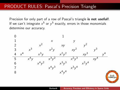
PRODUCT RULES: Pascal’s Precision Triangle
Precision for only part of a row of Pascal’s triangle is not useful!.If we can’t integrate x5 or y 5 exactly, errors in those monomialsdetermine our accuracy.
0 11 x y2 x2 xy y 2
3 x3 x2y xy 2 y 3
4 x4 x3y x2y 2 xy 3 y 4
5 x4y x3y 2 x2y 3 xy 4
6 x4y 2 x3y 3 x2y 4
7 x4y 3 x3y 4
8 x4y 4
Burkardt Accuracy, Precision and Efficiency in Sparse Grids
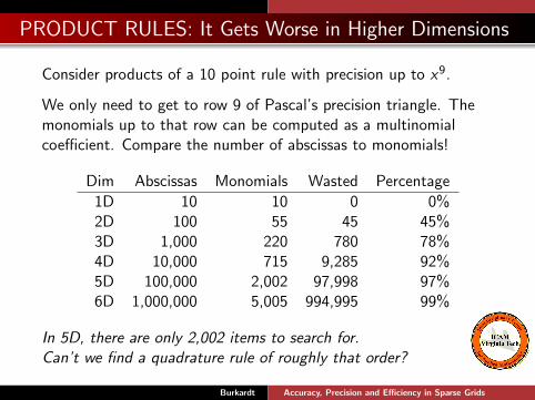
PRODUCT RULES: It Gets Worse in Higher Dimensions
Consider products of a 10 point rule with precision up to x9.
We only need to get to row 9 of Pascal’s precision triangle. Themonomials up to that row can be computed as a multinomialcoefficient. Compare the number of abscissas to monomials!
Dim Abscissas Monomials Wasted Percentage
1D 10 10 0 0%2D 100 55 45 45%3D 1,000 220 780 78%4D 10,000 715 9,285 92%5D 100,000 2,002 97,998 97%6D 1,000,000 5,005 994,995 99%
In 5D, there are only 2,002 items to search for.Can’t we find a quadrature rule of roughly that order?
Burkardt Accuracy, Precision and Efficiency in Sparse Grids
Accuracy, Precision and Efficiency in Sparse Grids
1 Introduction
2 Quadrature Rules in 1D
3 Product Rules for Higher Dimensions
4 Smolyak Quadrature
5 Covering Pascal’s Triangle
6 How Grids Combine
7 Sparse Grids in Action
8 Smoothness is Necessary
9 A Stochastic Diffusion Equation
10 Conclusion
Burkardt Accuracy, Precision and Efficiency in Sparse Grids
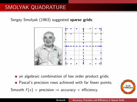
SMOLYAK QUADRATURE
Sergey Smolyak (1963) suggested sparse grids:
an algebraic combination of low order product grids;
Pascal’s precision rows achieved with far fewer points;
Smooth f (x) + precision ⇒ accuracy + efficiency.
Burkardt Accuracy, Precision and Efficiency in Sparse Grids
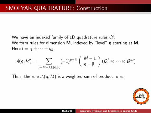
SMOLYAK QUADRATURE: Construction
We have an indexed family of 1D quadrature rules Qi .We form rules for dimension M, indexed by “level” q starting at M.Here i = i1 + · · ·+ iM .
A(q,M) =∑
q−M+1≤|i|≤q
(−1)q−|i|(
M − 1q − |i|
)(Qi1 ⊗ · · · ⊗ QiM )
Thus, the rule A(q,M) is a weighted sum of product rules.
Burkardt Accuracy, Precision and Efficiency in Sparse Grids
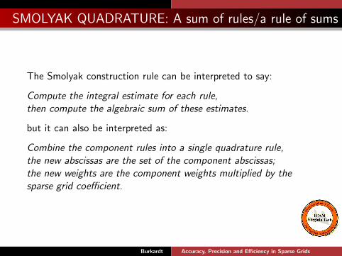
SMOLYAK QUADRATURE: A sum of rules/a rule of sums
The Smolyak construction rule can be interpreted to say:
Compute the integral estimate for each rule,then compute the algebraic sum of these estimates.
but it can also be interpreted as:
Combine the component rules into a single quadrature rule,the new abscissas are the set of the component abscissas;the new weights are the component weights multiplied by thesparse grid coefficient.
Burkardt Accuracy, Precision and Efficiency in Sparse Grids
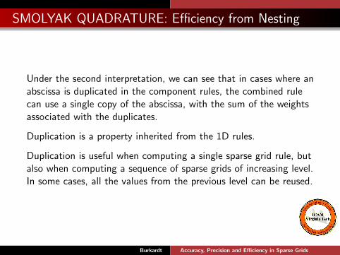
SMOLYAK QUADRATURE: Efficiency from Nesting
Under the second interpretation, we can see that in cases where anabscissa is duplicated in the component rules, the combined rulecan use a single copy of the abscissa, with the sum of the weightsassociated with the duplicates.
Duplication is a property inherited from the 1D rules.
Duplication is useful when computing a single sparse grid rule, butalso when computing a sequence of sparse grids of increasing level.In some cases, all the values from the previous level can be reused.
Burkardt Accuracy, Precision and Efficiency in Sparse Grids

SMOLYAK QUADRATURE: Using Clenshaw-Curtis
A common choice is 1D Clenshaw-Curtis rules.
We can make a nested family by choosing successive orders of 1, 3,5, 9, 17, ...
We wrote Qi to indicate the 1D quadrature rules indexed by alevel running 0, 1, 2, 3, and so on.
We will use a plain Qi to mean the 1D quadrature rules of order 1,3, 5, 9 and so on.
We will find it helpful to count abscissas.
Burkardt Accuracy, Precision and Efficiency in Sparse Grids
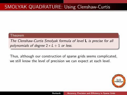
SMOLYAK QUADRATURE: Using Clenshaw-Curtis
Theorem
The Clenshaw-Curtis Smolyak formula of level L is precise for allpolynomials of degree 2 ∗ L + 1 or less.
Thus, although our construction of sparse grids seems complicated,we still know the level of precision we can expect at each level.
Burkardt Accuracy, Precision and Efficiency in Sparse Grids
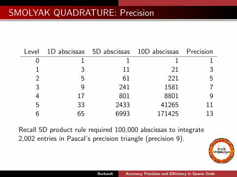
SMOLYAK QUADRATURE: Precision
Level 1D abscissas 5D abscissas 10D abscissas Precision
0 1 1 1 11 3 11 21 32 5 61 221 53 9 241 1581 74 17 801 8801 95 33 2433 41265 116 65 6993 171425 13
Recall 5D product rule required 100,000 abscissas to integrate2,002 entries in Pascal’s precision triangle (precision 9).
Burkardt Accuracy, Precision and Efficiency in Sparse Grids
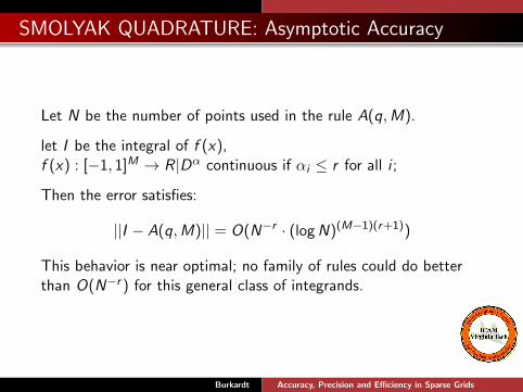
SMOLYAK QUADRATURE: Asymptotic Accuracy
Let N be the number of points used in the rule A(q,M).
let I be the integral of f (x),f (x) : [−1, 1]M → R|Dα continuous if αi ≤ r for all i ;
Then the error satisfies:
||I − A(q,M)|| = O(N−r · (log N)(M−1)(r+1))
This behavior is near optimal; no family of rules could do betterthan O(N−r ) for this general class of integrands.
Burkardt Accuracy, Precision and Efficiency in Sparse Grids
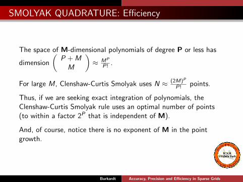
SMOLYAK QUADRATURE: Efficiency
The space of M-dimensional polynomials of degree P or less has
dimension
(P + M
M
)≈ MP
P! .
For large M, Clenshaw-Curtis Smolyak uses N ≈ (2M)P
P! points.
Thus, if we are seeking exact integration of polynomials, theClenshaw-Curtis Smolyak rule uses an optimal number of points(to within a factor 2P that is independent of M).
And, of course, notice there is no exponent of M in the pointgrowth.
Burkardt Accuracy, Precision and Efficiency in Sparse Grids
Accuracy, Precision and Efficiency in Sparse Grids
1 Introduction
2 Quadrature Rules in 1D
3 Product Rules for Higher Dimensions
4 Smolyak Quadrature
5 Covering Pascal’s Triangle
6 How Grids Combine
7 Sparse Grids in Action
8 Smoothness is Necessary
9 A Stochastic Diffusion Equation
10 Conclusion
Burkardt Accuracy, Precision and Efficiency in Sparse Grids
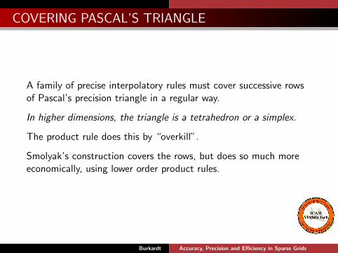
COVERING PASCAL’S TRIANGLE
A family of precise interpolatory rules must cover successive rowsof Pascal’s precision triangle in a regular way.
In higher dimensions, the triangle is a tetrahedron or a simplex.
The product rule does this by “overkill”.
Smolyak’s construction covers the rows, but does so much moreeconomically, using lower order product rules.
Burkardt Accuracy, Precision and Efficiency in Sparse Grids
COVERING PASCAL’S TRIANGLE
Let’s watch how this works for a family of 2D rules.
I’ve had to turn Pascal’s triangle sideways, to an XY grid. If wecount from 0, then box (I,J) represents x iy j .
Thus a row of Pascal’s triangle is now a diagonal of this plot.
The important thing to notice is the maximum diagonal that iscompletely covered. This is the precision of the rule.
We will see levels 0 through 4 and expect precisions 1 through 11by 2’s.
Burkardt Accuracy, Precision and Efficiency in Sparse Grids
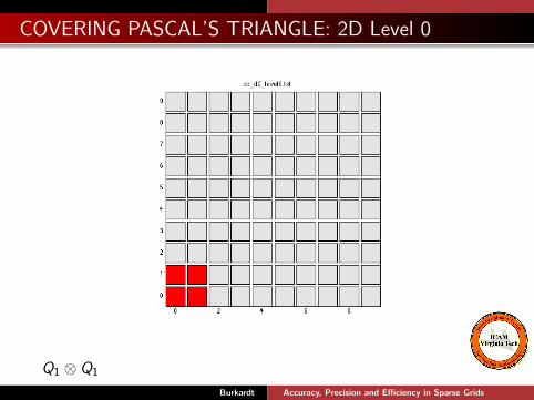
COVERING PASCAL’S TRIANGLE: 2D Level 0
Q1 ⊗ Q1
Burkardt Accuracy, Precision and Efficiency in Sparse Grids
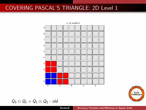
COVERING PASCAL’S TRIANGLE: 2D Level 1
Q3 ⊗ Q1 + Q1 ⊗ Q3 - old
Burkardt Accuracy, Precision and Efficiency in Sparse Grids
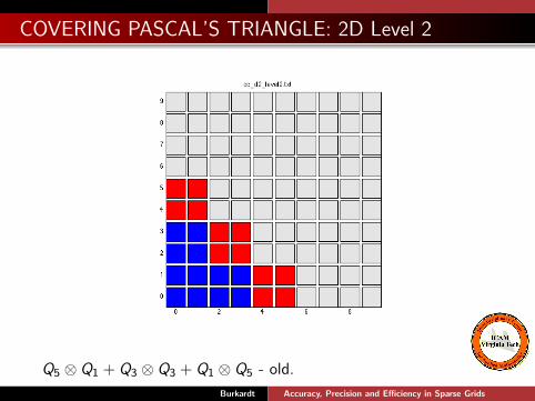
COVERING PASCAL’S TRIANGLE: 2D Level 2
Q5 ⊗ Q1 + Q3 ⊗ Q3 + Q1 ⊗ Q5 - old.
Burkardt Accuracy, Precision and Efficiency in Sparse Grids
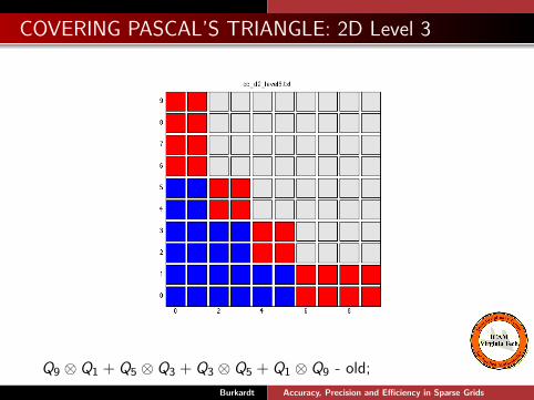
COVERING PASCAL’S TRIANGLE: 2D Level 3
Q9 ⊗ Q1 + Q5 ⊗ Q3 + Q3 ⊗ Q5 + Q1 ⊗ Q9 - old;
Burkardt Accuracy, Precision and Efficiency in Sparse Grids
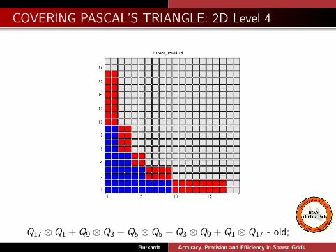
COVERING PASCAL’S TRIANGLE: 2D Level 4
Q17 ⊗ Q1 + Q9 ⊗ Q3 + Q5 ⊗ Q5 + Q3 ⊗ Q9 + Q1 ⊗ Q17 - old;
Burkardt Accuracy, Precision and Efficiency in Sparse Grids
Accuracy, Precision and Efficiency in Sparse Grids
1 Introduction
2 Quadrature Rules in 1D
3 Product Rules for Higher Dimensions
4 Smolyak Quadrature
5 Covering Pascal’s Triangle
6 How Grids Combine
7 Sparse Grids in Action
8 Smoothness is Necessary
9 A Stochastic Diffusion Equation
10 Conclusion
Burkardt Accuracy, Precision and Efficiency in Sparse Grids

HOW GRIDS COMBINE
We said that the Smolyak construction combines low order productrules, and that the result can be regarded as a single rule.
Let’s look at the construction of the Smolyak grid of level 4 in 2D.
Our construction will involve 1D rules of orders 1, 3, 5, 9 and 17,and product rules formed of these factors.
Because of nesting, every product rule we form will be a subset ofthe 17x17 full product grid.
Burkardt Accuracy, Precision and Efficiency in Sparse Grids
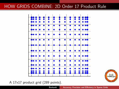
HOW GRIDS COMBINE: 2D Order 17 Product Rule
A 17x17 product grid (289 points).Burkardt Accuracy, Precision and Efficiency in Sparse Grids
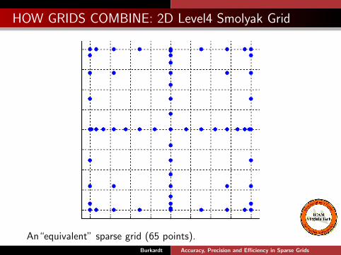
HOW GRIDS COMBINE: 2D Level4 Smolyak Grid
An“equivalent” sparse grid (65 points).Burkardt Accuracy, Precision and Efficiency in Sparse Grids

HOW GRIDS COMBINE
A(6, 2) =∑
6−2+1≤|i|≤6
(−1)6−|i|(
2− 16− |i|
)(Qi1 ⊗Qi2)
=−Q1 ⊗Q4 (Q1 ⊗ Q9)
−Q2 ⊗Q3 (Q3 ⊗ Q5)
−Q3 ⊗Q2 (Q5 ⊗ Q3)
−Q4 ⊗Q1 (Q9 ⊗ Q1)
+Q1 ⊗Q5 (Q1 ⊗ Q17)
+Q2 ⊗Q4 (Q3 ⊗ Q9)
+Q3 ⊗Q3 (Q5 ⊗ Q5)
+Q4 ⊗Q2 (Q9 ⊗ Q3)
+Q5 ⊗Q1 (Q17 ⊗ Q1)
Burkardt Accuracy, Precision and Efficiency in Sparse Grids
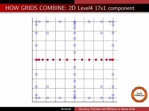
HOW GRIDS COMBINE: 2D Level4 17x1 component
Burkardt Accuracy, Precision and Efficiency in Sparse Grids

HOW GRIDS COMBINE: 2D Level4 9x3 component
Burkardt Accuracy, Precision and Efficiency in Sparse Grids

HOW GRIDS COMBINE: 2D Level4 5x5 component
Burkardt Accuracy, Precision and Efficiency in Sparse Grids
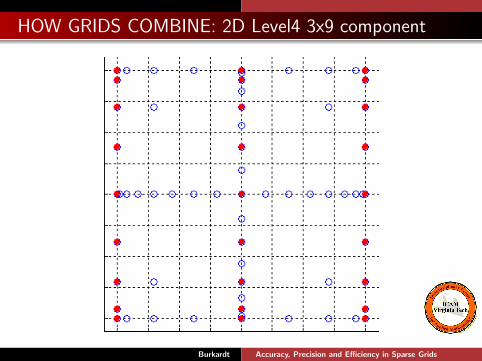
HOW GRIDS COMBINE: 2D Level4 3x9 component
Burkardt Accuracy, Precision and Efficiency in Sparse Grids
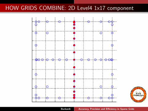
HOW GRIDS COMBINE: 2D Level4 1x17 component
Burkardt Accuracy, Precision and Efficiency in Sparse Grids
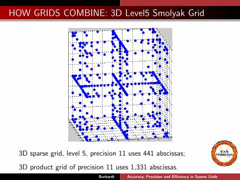
HOW GRIDS COMBINE: 3D Level5 Smolyak Grid
3D sparse grid, level 5, precision 11 uses 441 abscissas;
3D product grid of precision 11 uses 1,331 abscissas.Burkardt Accuracy, Precision and Efficiency in Sparse Grids
Accuracy, Precision and Efficiency in Sparse Grids
1 Introduction
2 Quadrature Rules in 1D
3 Product Rules for Higher Dimensions
4 Smolyak Quadrature
5 Covering Pascal’s Triangle
6 How Grids Combine
7 Sparse Grids in Action
8 Smoothness is Necessary
9 A Stochastic Diffusion Equation
10 Conclusion
Burkardt Accuracy, Precision and Efficiency in Sparse Grids
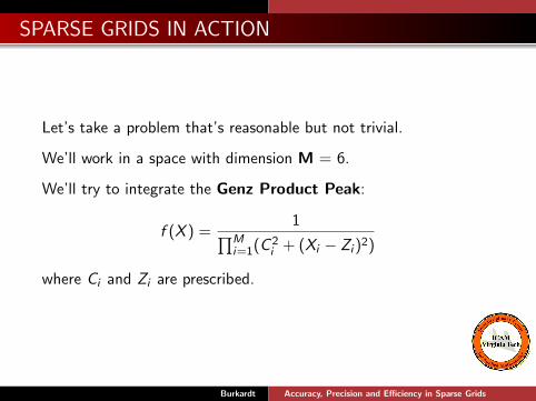
SPARSE GRIDS IN ACTION
Let’s take a problem that’s reasonable but not trivial.
We’ll work in a space with dimension M = 6.
We’ll try to integrate the Genz Product Peak:
f (X ) =1∏M
i=1(C 2i + (Xi − Zi )2)
where Ci and Zi are prescribed.
Burkardt Accuracy, Precision and Efficiency in Sparse Grids
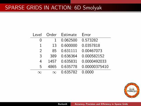
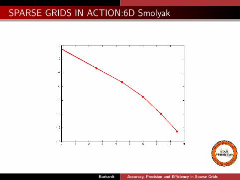
SPARSE GRIDS IN ACTION: 6D Smolyak
Level Order Estimate Error
0 1 0.062500 0.5732821 13 0.600000 0.03578182 85 0.631111 0.004670733 389 0.636364 0.0005821524 1457 0.635831 0.00004920335 4865 0.635778 0.00000375410
∞ ∞ 0.635782 0.0000
Burkardt Accuracy, Precision and Efficiency in Sparse Grids
SPARSE GRIDS IN ACTION:6D Smolyak
Burkardt Accuracy, Precision and Efficiency in Sparse Grids
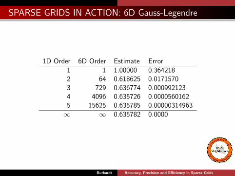
SPARSE GRIDS IN ACTION: 6D Gauss-Legendre
1D Order 6D Order Estimate Error
1 1 1.00000 0.3642182 64 0.618625 0.01715703 729 0.636774 0.0009921234 4096 0.635726 0.00005601625 15625 0.635785 0.00000314963
∞ ∞ 0.635782 0.0000
Burkardt Accuracy, Precision and Efficiency in Sparse Grids
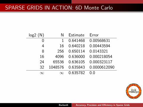
SPARSE GRIDS IN ACTION: 6D Monte Carlo
log2 (N) N Estimate Error
0 1 0.641468 0.005686314 16 0.640218 0.004435948 256 0.650114 0.0143321
16 4096 0.636000 0.00021805424 65536 0.636105 0.00032311732 1048576 0.635843 0.0000612090
∞ ∞ 0.635782 0.0
Burkardt Accuracy, Precision and Efficiency in Sparse Grids
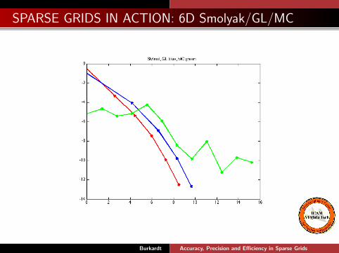
SPARSE GRIDS IN ACTION: 6D Smolyak/GL/MC
Burkardt Accuracy, Precision and Efficiency in Sparse Grids
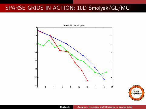
SPARSE GRIDS IN ACTION: 10D Smolyak/GL/MC
Burkardt Accuracy, Precision and Efficiency in Sparse Grids
SPARSE GRIDS IN ACTION: Thoughts
The graphs suggests that the accuracy behavior of the sparse gridrule is similar to the Gauss-Legendre rule, at least for this kind ofintegrand.
For 6 dimensions, the sparse grid rule is roughly 3 times as efficientas Gauss-Legendre, ( 4,865 abscissas versus 15,625 abscissas ).
Moving from 6 to 10 dimensions, the efficiency advantage is 60:(170,000 abscissas versus 9,700,000 abscissas).
The Gauss-Legendre product rule is beginning the explosive growthin abscissa count.
Burkardt Accuracy, Precision and Efficiency in Sparse Grids
Accuracy, Precision and Efficiency in Sparse Grids
1 Introduction
2 Quadrature Rules in 1D
3 Product Rules for Higher Dimensions
4 Smolyak Quadrature
5 Covering Pascal’s Triangle
6 How Grids Combine
7 Sparse Grids in Action
8 Smoothness is Necessary
9 A Stochastic Diffusion Equation
10 Conclusion
Burkardt Accuracy, Precision and Efficiency in Sparse Grids

Smoothness: A Few Words of Wisdom
”When good results are obtained in integrating a high-dimensionalfunction, we should conclude first of all that an especially tractableintegrand was tried and not that a generally successful method hasbeen found.
”A secondary conclusion is that we might have made a verygood choice in selecting an integration method to exploitwhatever features of f made it tractable.”
Art Owen, Stanford University.Burkardt Accuracy, Precision and Efficiency in Sparse Grids
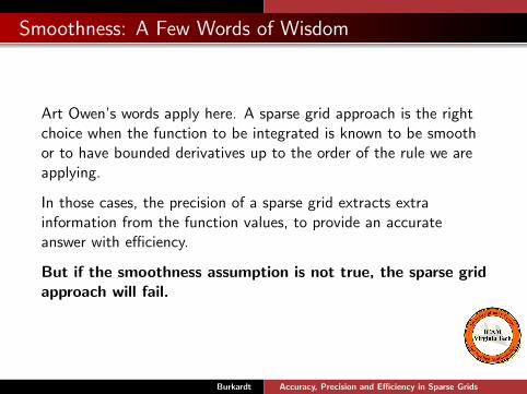
Smoothness: A Few Words of Wisdom
Art Owen’s words apply here. A sparse grid approach is the rightchoice when the function to be integrated is known to be smoothor to have bounded derivatives up to the order of the rule we areapplying.
In those cases, the precision of a sparse grid extracts extrainformation from the function values, to provide an accurateanswer with efficiency.
But if the smoothness assumption is not true, the sparse gridapproach will fail.
Burkardt Accuracy, Precision and Efficiency in Sparse Grids
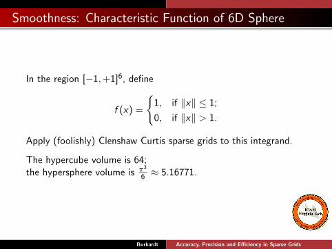
Smoothness: Characteristic Function of 6D Sphere
In the region [−1,+1]6, define
f (x) =
1, if ‖x‖ ≤ 1;
0, if ‖x‖ > 1.
Apply (foolishly) Clenshaw Curtis sparse grids to this integrand.
The hypercube volume is 64;the hypersphere volume is π3
6 ≈ 5.16771.
Burkardt Accuracy, Precision and Efficiency in Sparse Grids
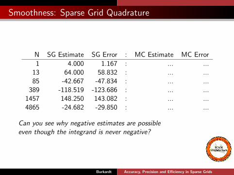
Smoothness: Sparse Grid Quadrature
N SG Estimate SG Error : MC Estimate MC Error
1 4.000 1.167 : ... ...13 64.000 58.832 : ... ...85 -42.667 -47.834 : ... ...
389 -118.519 -123.686 : ... ...1457 148.250 143.082 : ... ...4865 -24.682 -29.850 : ... ...
Can you see why negative estimates are possibleeven though the integrand is never negative?
Burkardt Accuracy, Precision and Efficiency in Sparse Grids
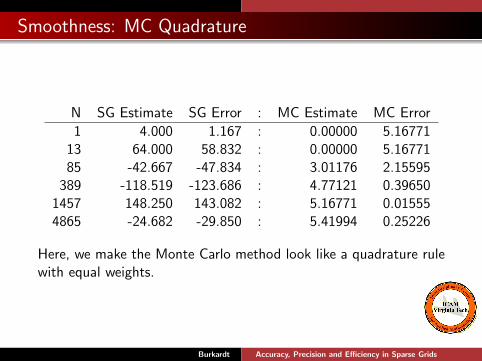
Smoothness: MC Quadrature
N SG Estimate SG Error : MC Estimate MC Error
1 4.000 1.167 : 0.00000 5.1677113 64.000 58.832 : 0.00000 5.1677185 -42.667 -47.834 : 3.01176 2.15595
389 -118.519 -123.686 : 4.77121 0.396501457 148.250 143.082 : 5.16771 0.015554865 -24.682 -29.850 : 5.41994 0.25226
Here, we make the Monte Carlo method look like a quadrature rulewith equal weights.
Burkardt Accuracy, Precision and Efficiency in Sparse Grids
Smoothness: MC Quadrature
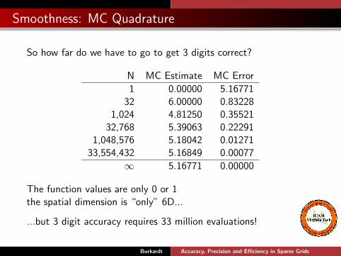
So how far do we have to go to get 3 digits correct?
N MC Estimate MC Error
1 0.00000 5.1677132 6.00000 0.83228
1,024 4.81250 0.3552132,768 5.39063 0.22291
1,048,576 5.18042 0.0127133,554,432 5.16849 0.00077
∞ 5.16771 0.00000
The function values are only 0 or 1the spatial dimension is “only” 6D...
...but 3 digit accuracy requires 33 million evaluations!
Burkardt Accuracy, Precision and Efficiency in Sparse Grids
Accuracy, Precision and Efficiency in Sparse Grids
1 Introduction
2 Quadrature Rules in 1D
3 Product Rules for Higher Dimensions
4 Smolyak Quadrature
5 Covering Pascal’s Triangle
6 How Grids Combine
7 Sparse Grids in Action
8 Smoothness is Necessary
9 A Stochastic Diffusion Equation
10 Conclusion
Burkardt Accuracy, Precision and Efficiency in Sparse Grids
Stochastic Diffusion
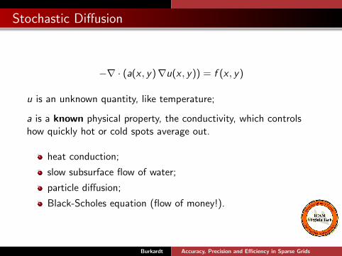
−∇ · (a(x , y)∇u(x , y)) = f (x , y)
u is an unknown quantity, like temperature;
a is a known physical property, the conductivity, which controlshow quickly hot or cold spots average out.
heat conduction;
slow subsurface flow of water;
particle diffusion;
Black-Scholes equation (flow of money!).
Burkardt Accuracy, Precision and Efficiency in Sparse Grids
Stochastic Diffusion: Uncertain Conductivity
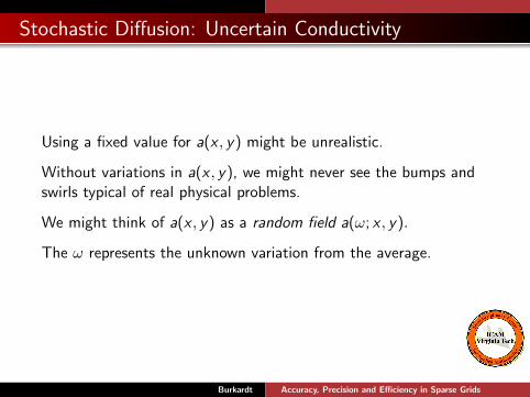
Using a fixed value for a(x , y) might be unrealistic.
Without variations in a(x , y), we might never see the bumps andswirls typical of real physical problems.
We might think of a(x , y) as a random field a(ω; x , y).
The ω represents the unknown variation from the average.
Burkardt Accuracy, Precision and Efficiency in Sparse Grids
Stochastic Diffusion: Uncertain Solution
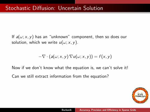
If a(ω; x , y) has an “unknown” component, then so does oursolution, which we write u(ω; x , y).
−∇ · (a(ω; x , y)∇u(ω; x , y)) = f (x , y)
Now if we don’t know what the equation is, we can’t solve it!
Can we still extract information from the equation?
Burkardt Accuracy, Precision and Efficiency in Sparse Grids
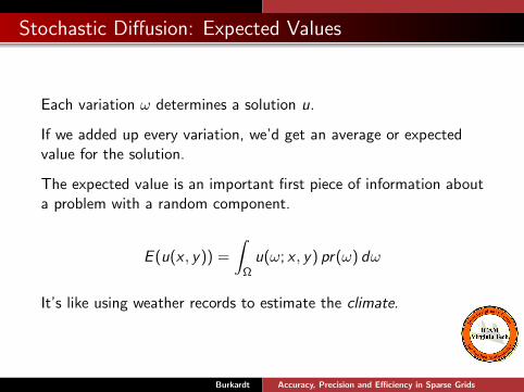
Stochastic Diffusion: Expected Values
Each variation ω determines a solution u.
If we added up every variation, we’d get an average or expectedvalue for the solution.
The expected value is an important first piece of information abouta problem with a random component.
E (u(x , y)) =
∫Ω
u(ω; x , y) pr(ω) dω
It’s like using weather records to estimate the climate.
Burkardt Accuracy, Precision and Efficiency in Sparse Grids
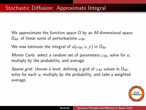
Stochastic Diffusion: Approximate Integral
We approximate the function space Ω by an M-dimensional spaceΩM , of linear sums of perturbations ωM .
We now estimate the integral of u(ωM ; x , y) in ΩM .
Monte Carlo: select a random set of parameters ωM , solve for u,multiply by the probability, and average.
Sparse grid: choose a level, defining a grid of ωM values in ΩM ,solve for each u, multiply by the probability, and take a weightedaverage.
Burkardt Accuracy, Precision and Efficiency in Sparse Grids
Stochastic Diffusion: Monte Carlo
0 0.5 1 1.5 2 2.5 3 3.5 4!12
!11
!10
!9
!8
!7
!6
!5
!4
!3
!2
Log10
(# points)
Log
10(L
2 e
rrors
)
Errors vs. # points
0 0.5 1 1.5 2 2.5 3 3.5 4!12
!11
!10
!9
!8
!7
!6
!5
!4
!3
!2
Log10
(# points)
Log
10(L
2 e
rrors
)
Errors vs. # points
0 0.5 1 1.5 2 2.5 3 3.5 4!12
!11
!10
!9
!8
!7
!6
!5
!4
!3
!2
Log10
(# points)
Log
10(L
2 e
rrors
)
Errors vs. # points
0 0.5 1 1.5 2 2.5 3 3.5 4!12
!11
!10
!9
!8
!7
!6
!5
!4
!3
!2
Log10
(# points)
Log
10(L
2 e
rrors
)
Errors vs. # points
N = 11 & L = 1/16
N = 11 & L = 1/4N = 11 & L = 1/2
N = 11 & L = 1/64
log 1
0(L2
erro
r)lo
g 10(
L2er
ror)
log 1
0(L2
erro
r)lo
g 10(
L2er
ror)
log10(# points) log10(# points)
log10(# points)log10(# points)
Anisotropic full tensor product with Gaussian abscissas (N = 11)
Isotropic Smolyak with Gaussian abscissas (N = 11)
Isotropic Smolyak with Clenshaw-Curtis abscissas (N = 11)
Anisotropic Smolyak with Clenshaw-Curtis abscissas (N = 11)
Anisotropic Smolyak with Gaussian abscissas (N = 11)
Monte Carlo
Monte Carlo
Monte Carlo
Monte Carlo
slope =!1/2slope =!1
slope =!1/2slope =!1
slope =!1/2slope =!1
slope =!1/2slope =!1
Burkardt Accuracy, Precision and Efficiency in Sparse Grids
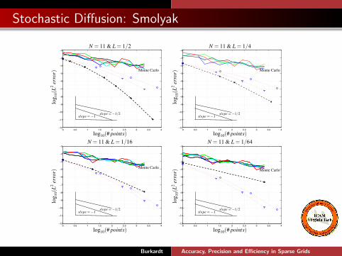
Stochastic Diffusion: Smolyak
0 0.5 1 1.5 2 2.5 3 3.5 4!12
!11
!10
!9
!8
!7
!6
!5
!4
!3
!2
Log10
(# points)
Log
10(L
2 e
rrors
)
Errors vs. # points
0 0.5 1 1.5 2 2.5 3 3.5 4!12
!11
!10
!9
!8
!7
!6
!5
!4
!3
!2
Log10
(# points)
Log
10(L
2 e
rrors
)
Errors vs. # points
0 0.5 1 1.5 2 2.5 3 3.5 4!12
!11
!10
!9
!8
!7
!6
!5
!4
!3
!2
Log10
(# points)
Log
10(L
2 e
rrors
)
Errors vs. # points
0 0.5 1 1.5 2 2.5 3 3.5 4!12
!11
!10
!9
!8
!7
!6
!5
!4
!3
!2
Log10
(# points)
Log
10(L
2 e
rrors
)
Errors vs. # points
N = 11 & L = 1/16
N = 11 & L = 1/4N = 11 & L = 1/2
N = 11 & L = 1/64
log 1
0(L2
erro
r)lo
g 10(
L2er
ror)
log 1
0(L2
erro
r)lo
g 10(
L2er
ror)
log10(# points) log10(# points)
log10(# points)log10(# points)
Anisotropic full tensor product with Gaussian abscissas (N = 11)
Isotropic Smolyak with Gaussian abscissas (N = 11)
Isotropic Smolyak with Clenshaw-Curtis abscissas (N = 11)
Anisotropic Smolyak with Clenshaw-Curtis abscissas (N = 11)
Anisotropic Smolyak with Gaussian abscissas (N = 11)
Monte Carlo
Monte Carlo
Monte Carlo
Monte Carlo
slope =!1/2slope =!1
slope =!1/2slope =!1
slope =!1/2slope =!1
slope =!1/2slope =!1
Burkardt Accuracy, Precision and Efficiency in Sparse Grids
Accuracy, Precision and Efficiency in Sparse Grids
1 Introduction
2 Quadrature Rules in 1D
3 Product Rules for Higher Dimensions
4 Smolyak Quadrature
5 Covering Pascal’s Triangle
6 How Grids Combine
7 Sparse Grids in Action
8 Smoothness is Necessary
9 A Stochastic Diffusion Equation
10 Conclusion
Burkardt Accuracy, Precision and Efficiency in Sparse Grids
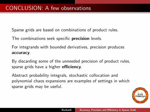
CONCLUSION: A few observations
Sparse grids are based on combinations of product rules.
The combinations seek specific precision levels.
For integrands with bounded derivatives, precision producesaccuracy.
By discarding some of the unneeded precision of product rules,sparse grids have a higher efficiency.
Abstract probability integrals, stochastic collocation andpolynomial chaos expansions are examples of settings in whichsparse grids may be useful.
Burkardt Accuracy, Precision and Efficiency in Sparse Grids
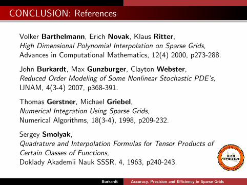
CONCLUSION: References
Volker Barthelmann, Erich Novak, Klaus Ritter,High Dimensional Polynomial Interpolation on Sparse Grids,Advances in Computational Mathematics, 12(4) 2000, p273-288.
John Burkardt, Max Gunzburger, Clayton Webster,Reduced Order Modeling of Some Nonlinear Stochastic PDE’s,IJNAM, 4(3-4) 2007, p368-391.
Thomas Gerstner, Michael Griebel,Numerical Integration Using Sparse Grids,Numerical Algorithms, 18(3-4), 1998, p209-232.
Sergey Smolyak,Quadrature and Interpolation Formulas for Tensor Products ofCertain Classes of Functions,Doklady Akademii Nauk SSSR, 4, 1963, p240-243.
Burkardt Accuracy, Precision and Efficiency in Sparse Grids