Accurate Infrared Tracking System for

Immersive Virtual Environments

Filipe Gaspar*

ADETTI-IUL / ISCTE-Lisbon University Institute, Portugal

Rafael Bastos

Vision-Box & ADETTI-IUL / ISCTE-Lisbon University Institute, Portugal

Miguel Sales Dias

Microsoft Language Development Center & ISCTE-Lisbon University Institute, Portugal

ABSTRACT

In large-scale immersive virtual reality (VR) environments such as a CAVE, one of the most

common interdisciplinary problems, crossing the fields of computer graphics and computer

vision, is to track the position of the head of user while he/she is immersed in this environment,

to reflect perspective changes in the synthetic stereoscopic images. In this paper, we describe the

theoretical foundations and engineering approach adopted in the development of an infrared-

optical tracking system, that show some advances in the current state-of-the art, especially

designed for large scale immersive Virtual Environments (VE) or Augmented Reality (AR)

settings. The system is capable of tracking independent retro-reflective markers arranged in a 3D

structure (artefact) in real time (25Hz), recovering all possible 6DOF. These artefacts can be

adjusted to the user’s stereo glasses to track his/her head pose while immersed, or can be used as

a 3D input device, for a rich human-computer interaction (HCI). The hardware configuration

consists in 4 shutter-synchronized cameras attached with band-pass infrared filters and

illuminated by infrared array-emitters. The system was specially designed to fit a room with

sizes of 5.7m x 2.7m x 3.4 m, which match the dimensions of the CAVE-Hollowspace of Lousal

in Portugal, where the system will be deployed in production. Pilot lab results have shown a

latency of 40 ms when simultaneously tracking the pose of two artefacts with 4 infrared markers,

achieving a frame-rate of 24.80 fps and showing a mean accuracy of 0.93mm/0.51º and a mean

precision of 0.19mm/0.04º, respectively, in overall translation/rotation, clearly fulfilling the

requirements initially defined.

Keywords: Three-Dimensional Graphics and Realism, Digitization and Image Capture,

Segmentation, Scene Analysis, Multimedia Information Systems, User Interfaces.

INTRODUCTION

During the last decade, Virtual and Augmented Reality technologies have became widely used in

several scientific and industrial fields. Large immersive virtual environments like the CAVE

(Cave Automatic Virtual Environment) (Cruz-Neira, 1992), can deliver to the users unique

immersive virtual experiences with rich HCI modalities that other environments cannot achieve.

In this context, through a collaboration of a large group of Portuguese and Brazilian entities

namely, institutional (Portuguese Ministry of Science, Grândola City Hall), academic (ISCTE-

IUL, IST, FCUL, PUC Rio), and industrial (SAPEC, Fundação Frederic Velge, Petrobrás,

Microsoft), the first large scale immersive virtual environment installed in Portugal,

“CaveHollowspace of Lousal” or “CaveH” in short (Dias, 2007), started its operation in the end

of 2007. The CaveH of Lousal (situated in the south of Portugal, near Grândola) is part of an

initiative of the National Agency for the Scientific and Technological Culture, in the framework

of the Live Science Centres network. CaveH aims at bringing to the educational, scientific and

industrial sectors in Portugal, the benefits of advanced technologies such as, immersive virtual

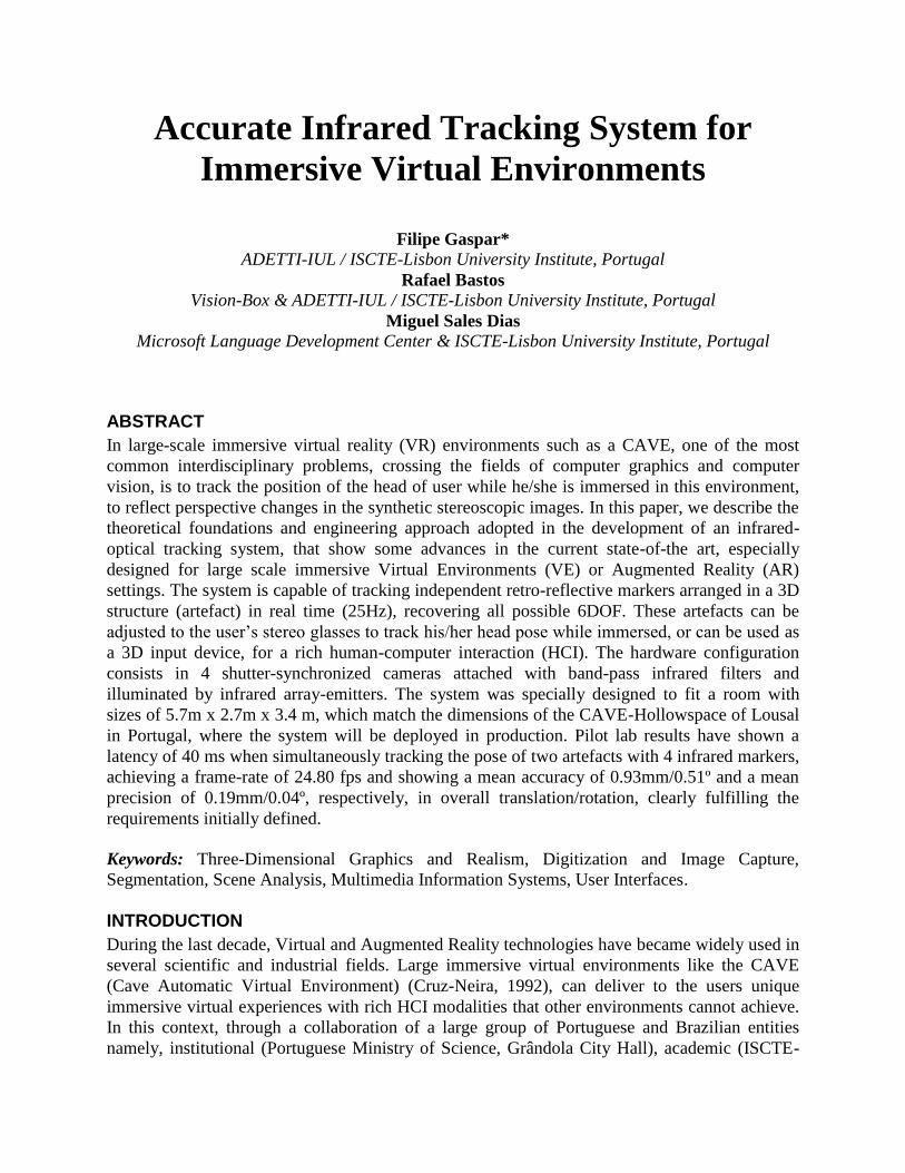
reality, digital mock-up and real-size interactive simulation. Its physical configuration is a 4-

sided cave assembling six projection planes (2 for the floor, 2 for the front, and 1 for each side)

in a U topology with 5.6 m wide, 2.7 m height and 3.4 m in each side (Figure 1), giving a field of

view of more than 180º, with a resolution of 8.2 mega pixel in stereoscopy for an audience of up

to 12 persons (where one is being tracked). It is worth mentioning that each front and floor

projection planes of the installation have 2 x 2 associated projectors (in a passive stereo set-up),

with a blending zone that creates the impression of a single projection plane each.

The range of critical industries where simulation and real-size digital mock-up observation are

imperative, extends the CaveH applicability to several fields such as, entertainment, aerospace,

natural resources exploration (oil, mining), industrial product design (automotive, architecture,

aeronautics), therapy (phobia, stress), etc. In most of these applications, the interaction with the

user is crucial to fulfil the application purpose.

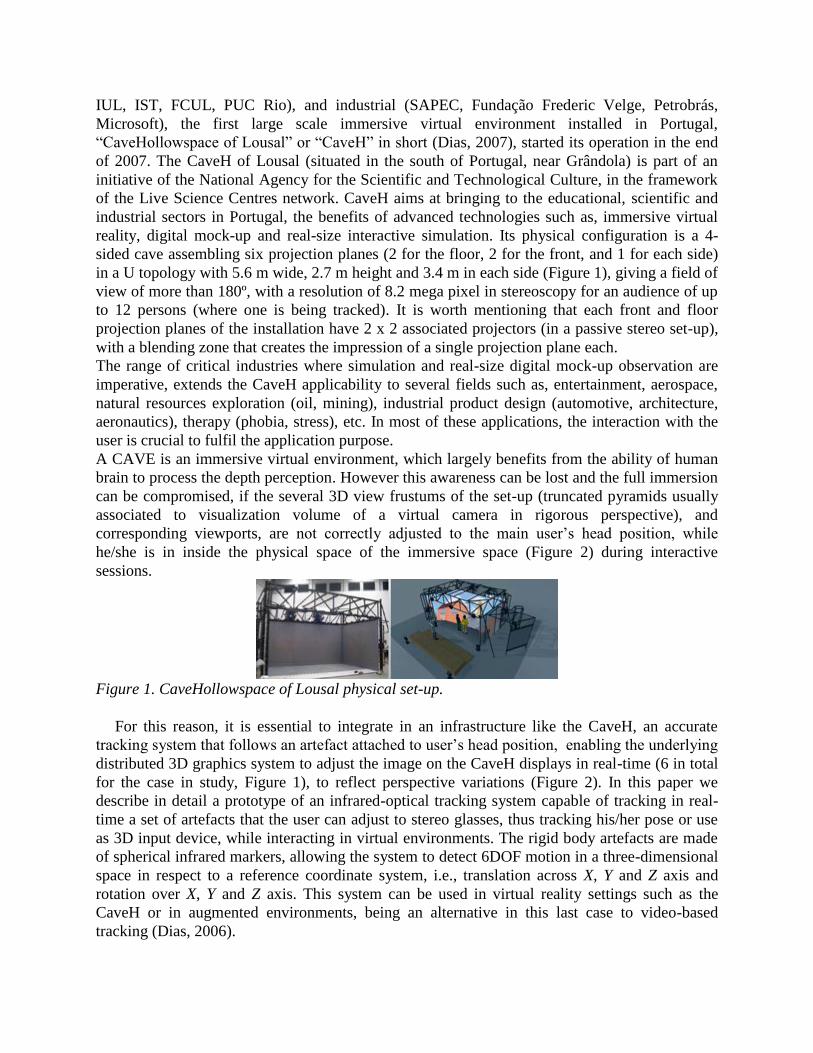
A CAVE is an immersive virtual environment, which largely benefits from the ability of human

brain to process the depth perception. However this awareness can be lost and the full immersion

can be compromised, if the several 3D view frustums of the set-up (truncated pyramids usually

associated to visualization volume of a virtual camera in rigorous perspective), and

corresponding viewports, are not correctly adjusted to the main user’s head position, while

he/she is in inside the physical space of the immersive space (Figure 2) during interactive

sessions.

Figure 1. CaveHollowspace of Lousal physical set-up.

For this reason, it is essential to integrate in an infrastructure like the CaveH, an accurate

tracking system that follows an artefact attached to user’s head position, enabling the underlying

distributed 3D graphics system to adjust the image on the CaveH displays in real-time (6 in total

for the case in study, Figure 1), to reflect perspective variations (Figure 2). In this paper we

describe in detail a prototype of an infrared-optical tracking system capable of tracking in real-

time a set of artefacts that the user can adjust to stereo glasses, thus tracking his/her pose or use

as 3D input device, while interacting in virtual environments. The rigid body artefacts are made

of spherical infrared markers, allowing the system to detect 6DOF motion in a three-dimensional

space in respect to a reference coordinate system, i.e., translation across X, Y and Z axis and

rotation over X, Y and Z axis. This system can be used in virtual reality settings such as the

CaveH or in augmented environments, being an alternative in this last case to video-based

tracking (Dias, 2006).

Figure 2. Dynamically adjustment of view frustums and viewpoints required to correctly display

images on several projection planes, when the user moves from a) to b).

The paper starts by summarizing the related state-of-the-art work in infrared and vision-based

tracking systems (Related Work) and then presents a System Overview of the chosen hardware

configuration as well as the developed software architecture. Subsequently, we describe the

proposed infrared Camera Calibration technique and present the in-house developed algorithms

that solve three common problems found in infrared tracking systems: Feature Segmentation and

Identification, 3D Reconstruction via Triangulation and Model Fitting. Then, in Results and

Discussion section, we present and discuss our results and, in last section we extract conclusions

and plan for future research directions.

RELATED WORK

Several commercial tracking systems can be found in the market. Vicon (2011) or ART (2011)

propose systems with configurations that usually allows 4 to 16 cameras, with update rates from

60Hz to 120Hz. However, due the high cost of these commercial solutions, we turned to the

scientific community and have analysed the literature regarding the availability of accurate and

precise algorithms to track independent rigid body markers and artefacts. We found out that the

multi or single camera systems, using infrared or vision-based tracking technologies share the

same problem formulation: the need of computing the position and orientation of a rigid body

target or artefact relatively to a reference coordinate system. To solve this problem a sufficient

number of geometric correspondences between a real feature in the world reference space and its

2D projection in the camera’s image space, is required. Several approaches to the tracking

problem can be found in the literature. In PTrack (Santos, 2006), a marker-based infrared single-

camera system is presented. Similar to ARToolKit (Kato, 1999), this contribution takes

advantage of a non-symmetric square geometric arrangement label in object space (an infrared

marker) and its correspondence in projected image space. PTrack uses an iterative approach to

twist the square label projection in order to derive a correct orientation, and then performs

iterative scaling to the label, to correct the position of the square infrared marker. Another single-

camera tracking contribution is ARTIC (Dias, 2004), where the marker design is based on colour

evaluation. Each marker has a different colour which can be segmented using vision-based-

techniques and a 3D artefact structure has been designed with five of such markers. The

algorithm used to estimate the artefact pose, is PosIT (DeMenthon, 1992). Analogous to Lowe

(1991), PosIT is an iterative algorithm but does not require an initial pose. The algorithm needs

four non-coplanar points as features in image space and the knowledge of the corresponding

object model points. The object pose is approximated through scaled orthographic projection.

Another well-known example of a multi-camera infrared tracking system is the ioTracker

(nowadays is a commercial system, even though it started as a research project) (Pintaric, 2007).

This system uses rigid body spherical infrared markers (targets) that take advantage of the

following constraint: every pair-wise Euclidean distance between features associated to markers,

is different and the artefacts construction is done to maximize the minimum difference between

these features’ pair-wise distances. By having several cameras, the feature information in several

image spaces is correlated via Epipolar Geometry (the geometry of stereoscopic projection) and

the 3D reconstructed feature in object space is performed via Singular Value Decomposition

(Golub, 1993). The pose estimation is a 3D-3D least square pose estimation problem (Arun,

1987) and requires the object model points and at least 3 reconstructed points to estimate a 6DOF

pose. In (Santos, 2010), an extension of PTrack system for multiple cameras is presented.

Several independent units of PTrack are combined to track several square infrared marker labels

via multiple cameras. Camera calibration is achieved via traditional techniques. The

breakthrough of this work is in the sensor fusion module, which receives tracking information

from PTrack units and groups it by label identification. The final 3D position of each marker is

obtaining by averaging the marker positions in each camera, projected in the world coordinate

system. Each label orientation is computed as the normal vector of the label, from the cross-

product of two perpendicular edges of the label. Our work has been largely influenced by the

ioTracker, especially in two specific algorithms: Multiple-View Correlation (see Section 6.1) and

Model Fitting, where we follow the complexity reduction approach proposed by Pintaric and

Kaufmann (Model Fitting Section) with two important modifications and advances, to avoid

superfluous computational time (for further details see Section Candidate Evaluation via

Artefact Correlation).

SYSTEM OVERVIEW

In order to develop a tracking system our first step was to create a comparative assessment

between different tracking technologies that can be used in immersive virtual environments such

as the CaveH, based on a clear definition of system requirements which are:

1. Real time update rate (at least 25 Hz, which is the maximum supported by affordable infrared

cameras);

2. Without major motion constraints: this means that the tracking technology shall be less

obtrusive as possible, allowing the user to interact with the CaveH environment through

several artefacts and enabling the best freedom of movement;

3. Robust to interference of the environment, that is, the technology chosen should not have

interferences with system materials and hardware (e.g. acoustic interference, electromagnetic

interference);

4. Without error accumulation in the estimated poses, that is, the accuracy of the estimated

artefact pose should be below 1 mm and 0.5º, respectively, for the overall translation (average

over the 3DOF in translation) and overall rotation (average over the 3DOF in rotation);

5. No significant drift of the estimated pose, that is, the precision of the estimated artefact 3D

pose (position and orientation) should be below 0.1mm and 0.1º, respectively, for the overall

translation (average over the 3DOF in translation) and overall rotation (average over the

3DOF in rotation).

In the following sub-sections we present an evaluation of several tracking technologies

regarding their performance and reliability (Tracking Technologies Assessment), followed by the

hardware components of our system (Hardware Setup) and the software architecture and

workflow. In Figure 3 is depicted a high level diagram representing the key concepts and the

CaveH technologies used to enable an immersive virtual environment.

Figure 3. Key concepts and CaveH technologies to enable immersion in a virtual reality

environment.

Tracking Technologies Assessment

In Table 1, we present a summarized comparison between the main advantages and drawbacks of

different available tracking technologies. By analysing this table, we can conclude that only

optical technology can cover all our specified requirements. However, this option highlights

three problems to be addressed: (1) line of sight occlusion; (2) ambient light interference; and (3)

infrared radiation in the environment, which we will tackle through the hardware configuration

chosen. Considering the nature of our problem (tracking artefacts poses in a room-sized

environment), an outside-in tracking approach is the best fit solution. Outside-in tracking

employs an external active sensor (usually a video camera) that senses artificial passive sources

or markers over the body of a person or on an artefact, and retrieves its pose in relation to a

reference coordinate system.

Table 1. Tracking technologies requirements comparison.

Technologies Accuracy and

precision

Real time

update rate

Robust to

interference

Motion

constraints

Additional

problems

Acoustic

Low, Low (centimetres,

degrees)

No (speed of sound

variation)

No

(acoustic

interference)

Yes

(line of sight

occlusion)

None

Electromagnetic

High, High

(sub-millimetre,

sub-degree)

Yes

(>100Hz)

No (interference with

metal objects) No

Small

working

volume

Inertial

High, Low (error

accumulation)

Yes (>100Hz)

No (graviton

interference) No

Limited by

cabling

Mechanical

High, High

(sub-millimetre,

sub-degree)

Yes (100Hz)

Yes

Yes (mechanical

arm paradigm

Small

working

volume

Optical

High, High (sub-millimetre,

sub-degree)

Yes

(>=25Hz)

No

(ambient light and

infrared radiation)

Yes (line of sight

occlusion)

None

Hardware Setup

Once the technology to be used has been defined, the hardware setup was chosen based on a

strategy to minimize costs, without compromising the system reliability and performance and the

specified requirements.

Cameras

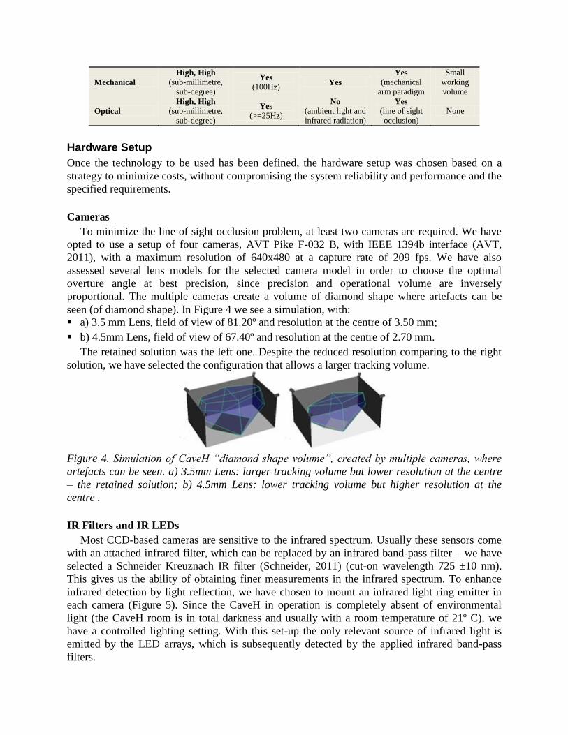
To minimize the line of sight occlusion problem, at least two cameras are required. We have

opted to use a setup of four cameras, AVT Pike F-032 B, with IEEE 1394b interface (AVT,

2011), with a maximum resolution of 640x480 at a capture rate of 209 fps. We have also

assessed several lens models for the selected camera model in order to choose the optimal

overture angle at best precision, since precision and operational volume are inversely

proportional. The multiple cameras create a volume of diamond shape where artefacts can be

seen (of diamond shape). In Figure 4 we see a simulation, with:

a) 3.5 mm Lens, field of view of 81.20º and resolution at the centre of 3.50 mm;

b) 4.5mm Lens, field of view of 67.40º and resolution at the centre of 2.70 mm.

The retained solution was the left one. Despite the reduced resolution comparing to the right

solution, we have selected the configuration that allows a larger tracking volume.

Figure 4. Simulation of CaveH “diamond shape volume”, created by multiple cameras, where

artefacts can be seen. a) 3.5mm Lens: larger tracking volume but lower resolution at the centre

– the retained solution; b) 4.5mm Lens: lower tracking volume but higher resolution at the

centre .

IR Filters and IR LEDs

Most CCD-based cameras are sensitive to the infrared spectrum. Usually these sensors come

with an attached infrared filter, which can be replaced by an infrared band-pass filter – we have

selected a Schneider Kreuznach IR filter (Schneider, 2011) (cut-on wavelength 725 ±10 nm).

This gives us the ability of obtaining finer measurements in the infrared spectrum. To enhance

infrared detection by light reflection, we have chosen to mount an infrared light ring emitter in

each camera (Figure 5). Since the CaveH in operation is completely absent of environmental

light (the CaveH room is in total darkness and usually with a room temperature of 21º C), we

have a controlled lighting setting. With this set-up the only relevant source of infrared light is

emitted by the LED arrays, which is subsequently detected by the applied infrared band-pass

filters.

Shutter Controller

In order to synchronize the cameras frame grabbers, we need to use a shutter controller. We

have opted by a National Instruments USB shutter controller NI-USB6501 (NI, 2011), a digital

and programmable device that triggers camera’s capture on varying or static periods of time.

Artefacts

Artefacts are made of a set of infrared markers arranged in space with known pair-wise

Euclidean distances in a pre-defined structure. Each artefact is a unique object with a detectable

pose within a tracking volume. We have opted by passive retro-reflective markers instead of

active markers because the last ones require an electric source, which would become more

expensive, heavy and intrusive. Our lab-made markers are built from plastic spheres with 20 mm

of radius and covered with retro-reflective self-adhesive paper. We have chosen spheres since it

is a geometric form that allows an approximation to an isotropic reflection system.

Figure 5. Hardware components of the Infrared Camera system. a) AVT Pike Camera; b)

Infrared LED emitter; c) Shutter controller; d) Artefact for IR tracking.

Software Architecture and Process Workflow

Our software architecture comprises a real-time and threaded oriented pipeline. The diagram in

Figure 6 illustrates the full real-time infrared tracking pipeline process since multiple frames

(one per camera), synchronously reach the application to generate the final output: the pose of

each target in a known reference coordinate system.

However, two other important steps are done previously during an off-line stage:

Camera calibration – For each camera, we determine its intrinsic parameters (focal length,

the principal point, pixel scale factors in the image domain and the non-linear radial and

tangential distortion parameters), and extrinsic parameters (position and orientation in relation to

a reference coordinate system);

Artefact calibration – For each artefact structure, we compute the Euclidean distances

between each pair of markers. This procedure allows us to use artefacts with different and non-

pre-defined topologies (under some constraints, see Candidate Evaluation via Artefact

Correlation Section) and overcomes the precision error in their construction. A “reference pose”

is also computed for comparison with poses retrieved by application.

Each on-line pipeline cycle in Figure 6 starts when multiple frames are grabbed by the

application (Multiple Video Input). For each frame an image segmentation algorithm identifies

the 2D image coordinates of every blob feature, i.e. the 3D real infrared marker projected in the

image, and recovers its centre and radius (Feature Segmentation). Through epipolar geometry

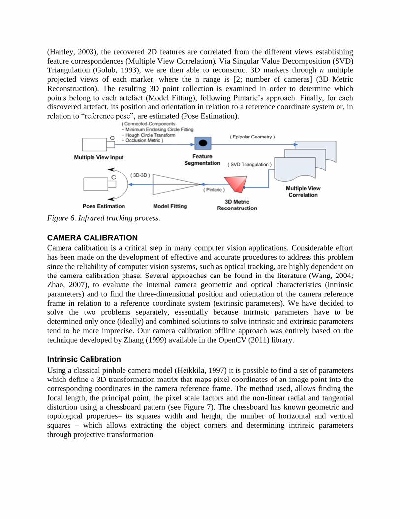
(Hartley, 2003), the recovered 2D features are correlated from the different views establishing

feature correspondences (Multiple View Correlation). Via Singular Value Decomposition (SVD)

Triangulation (Golub, 1993), we are then able to reconstruct 3D markers through n multiple

projected views of each marker, where the n range is [2; number of cameras] (3D Metric

Reconstruction). The resulting 3D point collection is examined in order to determine which

points belong to each artefact (Model Fitting), following Pintaric’s approach. Finally, for each

discovered artefact, its position and orientation in relation to a reference coordinate system or, in

relation to “reference pose”, are estimated (Pose Estimation).

Figure 6. Infrared tracking process.

CAMERA CALIBRATION

Camera calibration is a critical step in many computer vision applications. Considerable effort

has been made on the development of effective and accurate procedures to address this problem

since the reliability of computer vision systems, such as optical tracking, are highly dependent on

the camera calibration phase. Several approaches can be found in the literature (Wang, 2004;

Zhao, 2007), to evaluate the internal camera geometric and optical characteristics (intrinsic

parameters) and to find the three-dimensional position and orientation of the camera reference

frame in relation to a reference coordinate system (extrinsic parameters). We have decided to

solve the two problems separately, essentially because intrinsic parameters have to be

determined only once (ideally) and combined solutions to solve intrinsic and extrinsic parameters

tend to be more imprecise. Our camera calibration offline approach was entirely based on the

technique developed by Zhang (1999) available in the OpenCV (2011) library.

Intrinsic Calibration

Using a classical pinhole camera model (Heikkila, 1997) it is possible to find a set of parameters

which define a 3D transformation matrix that maps pixel coordinates of an image point into the

corresponding coordinates in the camera reference frame. The method used, allows finding the

focal length, the principal point, the pixel scale factors and the non-linear radial and tangential

distortion using a chessboard pattern (see Figure 7). The chessboard has known geometric and

topological properties– its squares width and height, the number of horizontal and vertical

squares – which allows extracting the object corners and determining intrinsic parameters

through projective transformation.

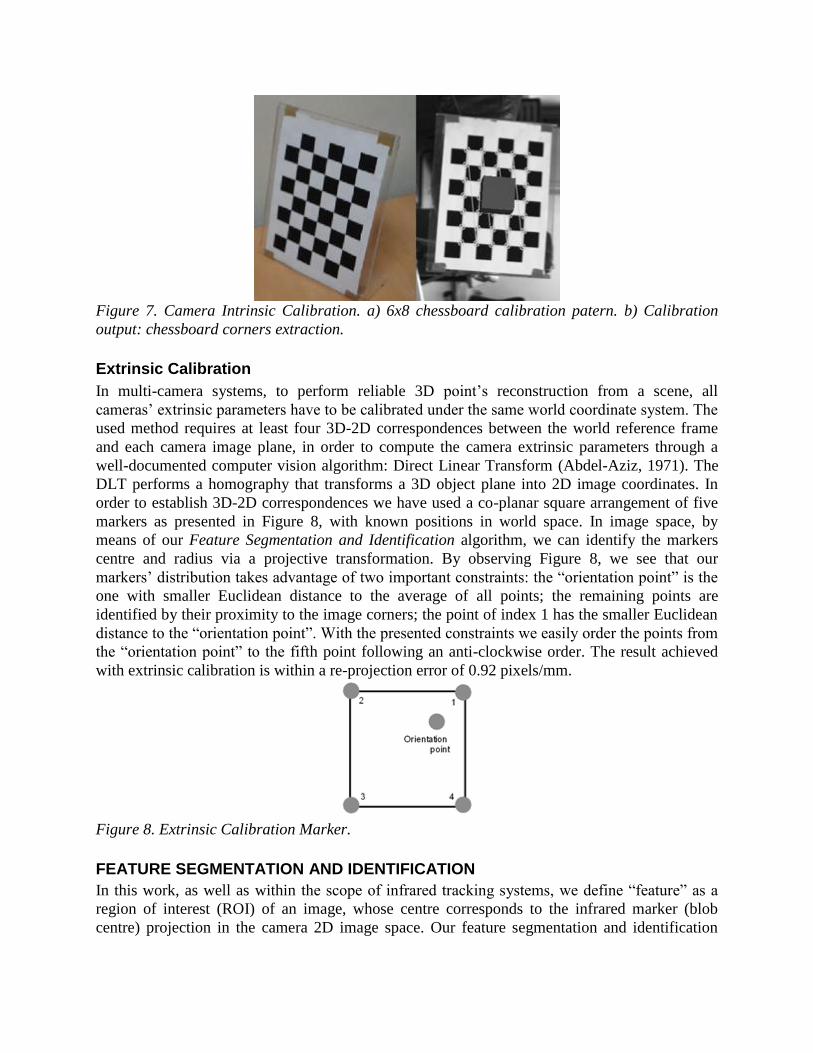
Figure 7. Camera Intrinsic Calibration. a) 6x8 chessboard calibration patern. b) Calibration

output: chessboard corners extraction.

Extrinsic Calibration

In multi-camera systems, to perform reliable 3D point’s reconstruction from a scene, all

cameras’ extrinsic parameters have to be calibrated under the same world coordinate system. The

used method requires at least four 3D-2D correspondences between the world reference frame

and each camera image plane, in order to compute the camera extrinsic parameters through a

well-documented computer vision algorithm: Direct Linear Transform (Abdel-Aziz, 1971). The

DLT performs a homography that transforms a 3D object plane into 2D image coordinates. In

order to establish 3D-2D correspondences we have used a co-planar square arrangement of five

markers as presented in Figure 8, with known positions in world space. In image space, by

means of our Feature Segmentation and Identification algorithm, we can identify the markers

centre and radius via a projective transformation. By observing Figure 8, we see that our

markers’ distribution takes advantage of two important constraints: the “orientation point” is the

one with smaller Euclidean distance to the average of all points; the remaining points are

identified by their proximity to the image corners; the point of index 1 has the smaller Euclidean

distance to the “orientation point”. With the presented constraints we easily order the points from

the “orientation point” to the fifth point following an anti-clockwise order. The result achieved

with extrinsic calibration is within a re-projection error of 0.92 pixels/mm.

Figure 8. Extrinsic Calibration Marker.

FEATURE SEGMENTATION AND IDENTIFICATION

In this work, as well as within the scope of infrared tracking systems, we define “feature” as a

region of interest (ROI) of an image, whose centre corresponds to the infrared marker (blob

centre) projection in the camera 2D image space. Our feature segmentation and identification

algorithm comprises several techniques to approximate blobs to circles recovering the feature’s

radius and centre.

Feature Segmentation through non-Destructive Threshold

After acquisition, the first image processing operation is a non-destructive image thresholding.

Since our work environment is lighting controlled and most of information is filtered by infrared

filters, we have used a threshold operation to eliminate noise and discard possible false artefacts

in the image. The output of the IR camera is a grey-scale image where the retro-reflective

markers have extremely high value of luminance (>65% of the maximum value). It is

straightforward to segment our features establishing a static threshold value (discovered

experimentally), where the pixels with luminance value below the threshold are forced to zero

(Figure 9). We have decided to use a non-destructive operation because in an algorithm used

later in our pipeline, the Hough Circle Transform (Kimme, 1975), the gradient information will

be extremely useful to accelerate circles searching.

Feature Identification

A classic approach to identify the retro-reflective markers in image space is the adoption of

Hough Circle Transform (HCT) (Kimme, 1975; Duda, 1972). HTC is a well-known technique to

find geometric primitives in an image (in our case, circles). The principle of this technique is to

transform the image space into a tri-dimensional accumulator, where each entry of the

accumulator is a potential circle parameterized by its centre (x, y coordinates) and radius. The

local-maxima entries on the accumulator will be the retrieved circles. Our features can assume a

wide range of radii in the image (especially if the image space has partially-occluded features),

which turns the Hough accumulation highly demanding, in terms of memory, to be applied in a

real-time application with the robustness and the precision needed. Therefore, instead of

applying HCT to the whole image (640 x 480 of resolution), our feature identification algorithm

consists in a combination of one technique to identify ROIs containing features (Connected-

Components Algorithm) and one decision metric (Occlusion Metric), to select the best algorithm

to be applied to the image to recover the features centres and radius from two possible algorithms

(Minimum Enclosing Circle Fitting or Hough Circle Transform), depending on whether occluded

features exist or not. For the HCT algorithm we use a bi-dimensional accumulator approach

(Kimme, 1975). The feature segmentation workflow can be seen in Figure 9.

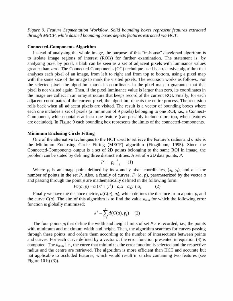
Figure 9. Feature Segmentation Workflow. Solid bounding boxes represent features extracted

through MECF, while dashed bounding boxes depicts features extracted via HCT.

Connected-Components Algorithm

Instead of analysing the whole image, the purpose of this “in-house” developed algorithm is

to isolate image regions of interest (ROIs) for further examination. The statement is: by

analysing pixel by pixel, a blob can be seen as a set of adjacent pixels with luminance values

greater than zero. The Connected-Components (CC) technique used is a recursive algorithm that

analyses each pixel of an image, from left to right and from top to bottom, using a pixel map

with the same size of the image to mark the visited pixels. The recursion works as follows. For

the selected pixel, the algorithm marks its coordinates in the pixel map to guarantee that that

pixel is not visited again. Then, if the pixel luminance value is larger than zero, its coordinates in

the image are collect in an array structure that keeps record of the current ROI. Finally, for each

adjacent coordinates of the current pixel, the algorithm repeats the entire process. The recursion

rolls back when all adjacent pixels are visited. The result is a vector of bounding boxes where

each one includes a set of pixels (a minimum of 9 pixels) belonging to one ROI, i.e., a Connect-

Component, which contains at least one feature (can possibly include more too, when features

are occluded). In Figure 9 each bounding box represents the limits of the connected-components.

Minimum Enclosing Circle Fitting

One of the alternative techniques to the HCT used to retrieve the feature’s radius and circle is

the Minimum Enclosing Circle Fitting (MECF) algorithm (Fitzgibbon, 1995). Since the

Connected-Components output is a set of 2D points belonging to the same ROI in image, the

problem can be stated by defining three distinct entities. A set of n 2D data points, P:

1

n

i iP p (1)

Where pi is an image point defined by its x and y pixel coordinates, (xi, yi), and n is the

number of points in the set P. Also, a family of curves, Fc (a, p), parameterized by the vector a

and passing through the point p are mathematically defined in the following form: 2 2

1 2 3 4( , ) ( )Fc a p a x y a x a y a (2)

Finally we have the distance metric, d(C(a), pi), which defines the distance from a point pi and

the curve C(a). The aim of this algorithm is to find the value amin for which the following error

function is globally minimized:

2

1

( ( ), )n

i

i

d C a p (3)

The four points pi that define the width and height limits of set P are recorded, i.e., the points

with minimum and maximum width and height. Then, the algorithm searches for curves passing

through these points, and orders them according to the number of intersections between points

and curves. For each curve defined by a vector a, the error function presented in equation (3) is

computed. The amin, i.e., the curve that minimizes the error function is selected and the respective

radius and the centre are retrieved. The algorithm is more efficient than HCT and accurate but

not applicable to occluded features, which would result in circles containing two features (see

Figure 10 b) (3)).

Occlusion Metric

Having two different techniques able to find feature’s radius and centre, we have decided to

add to our feature identification workflow an occlusion metric in order to determine whether or

not a ROI of the image has occlusions, and select the appropriate technique (MECF or HCT) to

apply in real-time.

Figure 10. Occluded and normal features comparison. a) Single feature example. b) Overlapped

features example. The three algorithmic phases in feature identification algorithm can be

observed: (1) original feature; (2) ROI in the image delimited by a bounding box; (3) MECF

with retrieved centre and radius.

During the development of our feature identification technique, we have observed several

proprieties regarding the outputs of both CC and MECF algorithms which allows us to

distinguish between “normal and “occluded” features. Examples, quite evident in Figure 10, and

are: occluded features usually show a lower percentage of white pixels inside the bounding box;

in occlusion cases, MECF area is normally larger than the bounding box area; occluded features

normally have a higher difference between bounding box width and height sizes; etc.

Considering these observations, we have performed a series of test cases, analysing both the

image bounding box defined by the CC algorithm and the MECF output, aiming to label features

in two distinct categories: “occluded” or “normal”. The performed tests comprised 200 different

samples, with 50% of the samples being the output from “normal” features cases and the

remaining samples, the output from “occluded” features cases. As a result of the performed tests,

we have proposed an empirical occlusion metric, comprising five rules in an OR logic operation,

to label features as “occluded” when:

1. Its bounding box retrieved by CC algorithm has less than 65% of white pixels;

2. The bounding box has a width and height difference greater than 1.5 pixels;

3. The MECF and ROI radius difference is greater than 0.9 pixels;

4. MEFC and bounding box area difference is greater than 60 pixels;

5. MEFC circle exceeds the ROI limits in more than 2.5 pixels.

Although we need to run MECF always to verify the last three rules, this strategy of using

HCT depending on the Occlusion Metric results, allows us saving 10.06 ms (see Results and

Discussion Section) per frame with a robustness of 97%, since MECF is faster and accurate but

only HCT is applicable to overlapped features.

3D RECONSTRUCTION VIA TRIANGULATION

Once identified the feature’s position in different views, the subsequent problem is to use these

information to reconstruct the markers position in 3D-scene space. In this section we cover the

geometry of several perspective views. First, we clarify how to establish correspondences across

imaged features in different views by using epipolar geometry (Hartley, 2003): we call it

Multiple View Correlation. Therefore, having groups of correspondent features, we present our

3D metric reconstruction to recover the marker position in 3D space via Singular Value

Decomposition (SVD) (Golub, 1993), the 3D Metric Reconstruction (Dias, 2007).

Multiple View Correlation

A useful and widely used mathematical technique to solve feature’s correlation from two or more

views is epipolar geometry (Hartley, 2003). The epipolar geometry theory defines that a 3D

point, X, imaged on the first camera view of a stereo pair, as x1 restricts the position of the

correspondent point x2 in the second camera view to a line (epipolar line), if we know the

extrinsic parameters of the stereoscopic camera system. This allows us to discard features as

possible correspondences whose distance to the epipolar line are above a certain threshold. Our

multiple-view correlation is based in this constraint and works as follows. We define a set of

stereo pairs between the reference camera the camera with most features in the current frame)

and the remaining ones. For every stereo pair and for each feature in the first view (reference

camera image), we compute the distance between the features centres in the second view and the

epipolar line that corresponds to the feature in the first view. All features with a distance above

our threshold are discarded. The corresponding feature is the one with the smallest distance to

the epipolar line. The result is a set of feature correspondences between the reference camera and

the remaining ones which can be merged giving a Multiple-View Correlation.

3D Metric Reconstruction

By setting a well-known camera topology during the camera calibration step and by establishing

optimal feature’s correlation through multiple view correlation, we are able to perform the 3D

metric reconstruction of the artefact. This process can be obtained in two different methods: by

triangulation or via SVD. When we have correspondences between only two views, we can use

triangulation instead of SVD to obtain the 3D point location, i.e., the 3D point can be computed

directly through epipolar geometry as the intersection of rays fired from the camera positions that

hit the corresponding image points and that intersect the 3D point. This analytic method is

clearly faster than using SVD. However, the line intersection problem can lead us to numerical

instability and subsequently to numerical indeterminacies which affect system stability. Having

several views for a given feature correspondence, several possible solutions for the

reconstruction derive from epipolar geometry and we are left with a set of linear equations that

can be solved to compute a metric reconstruction for each artefact feature via SVD (presented

also in (Dias, 2007)). The SVD usually denotes that a matrix A, can be decomposed as A = VɅU.

Using each camera’s intrinsic and extrinsic parameters, we stack into matrix A the existing

information for each i view (2D point location – x, y). Solving the A matrix by SVD and

retaining the last row of the V matrix, the reconstruction point coordinates (x, y, z) are the

singular values in Ʌ . The matrices sizes vary with the number of views used to reconstruction

the 3D points coordinates: A[2i x 4]; V[2i x 2i]; Ʌ [2i x 4]; U[4x4]. After testing both solutions in the two

viewing scenarios, we have decided to preserve the system reliability using the SVD technique,

despite the computational cost.

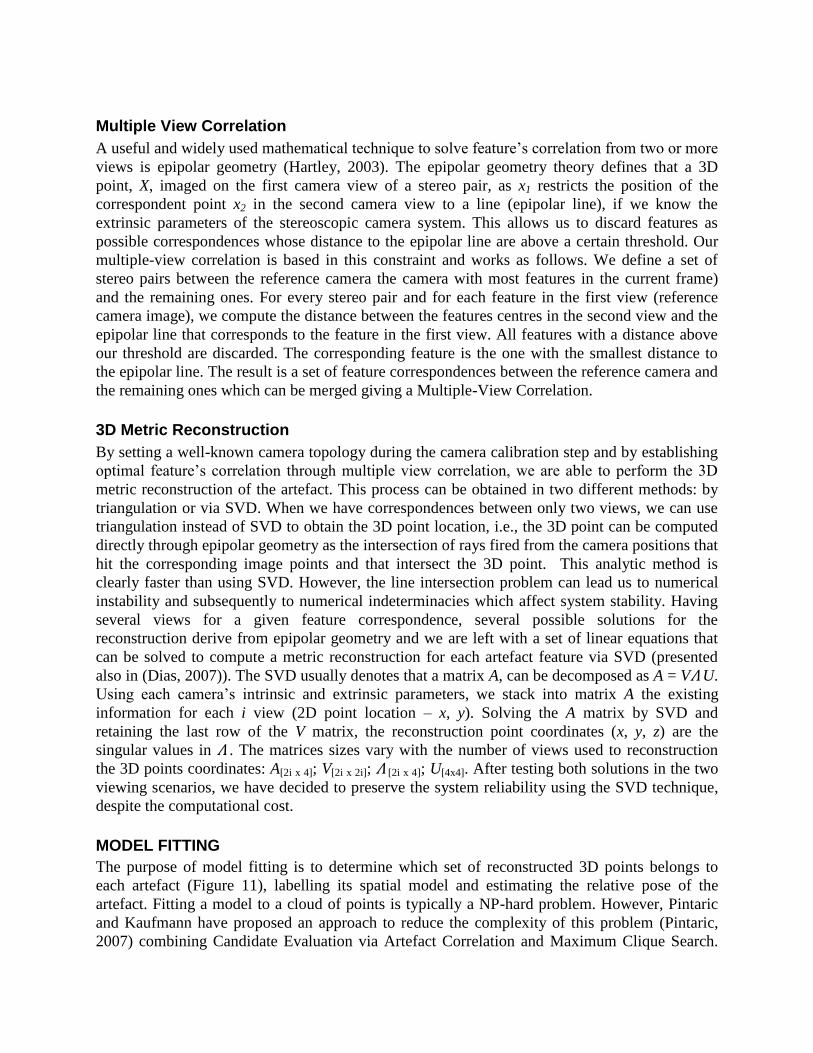
MODEL FITTING

The purpose of model fitting is to determine which set of reconstructed 3D points belongs to

each artefact (Figure 11), labelling its spatial model and estimating the relative pose of the

artefact. Fitting a model to a cloud of points is typically a NP-hard problem. However, Pintaric

and Kaufmann have proposed an approach to reduce the complexity of this problem (Pintaric,

2007) combining Candidate Evaluation via Artefact Correlation and Maximum Clique Search.

Our model fitting technique is largely influenced by Pintaric and Kaufmann. In the following

sections the technique is presented, focusing in our proposed improvements.

Figure 11. Rigid body artefacts. a) 6 DOF artefact used as 3D input device. b) 3 DOF artefact

attached to user’s stereo glasses.

Candidate Evaluation via Artefact Correlation

The candidate evaluation goal is to decide which points are “good candidates” to belong to the

specific artefacts. The metric used to compare pairs of 3D points is the Euclidean distance

between them, where we can take advantage of three important constraints: artefacts are rigid-

body objects with constant Euclidean distances between pair-wise markers; since we control the

artefacts construction, its design can be done to maximize the minimum difference between

Euclidean distances across all targets; knowing the minimum Euclidean distance detectable by

our system we maintain the previous constraint above this value. This Euclidean distance

constraint does not allow arbitrarily designed artefacts but, according to Pintaric (2007), the

computational complexity reduction that arises is worthwhile.

Figure 12. Candidate Evaluation workflow.

The candidate evaluation technique is divided into two phases (see Figure 12). For each

artefact, an offline calibration process (0. Calibration) is needed in order to construct a

Correlation Score Look-up Table (CSLT) with all artefact Euclidean distances between all pair-

wise markers, given the N distances [d0, ..., dN]. Let’s follow the example of artefact depicted in

Figure 12 where N = 6. At runtime (Online), for each system pipeline cycle, an Euclidean

Distance Matrix (EDM) of size M x M is constructed, containing distances between all pairs of

the M points reconstructed (M = 8 in the given example). For each calibrated artefact, a

Correlation Score Matrix (CSM) of size N x N is computed (1.Correlation). Each entry of CSM

corresponds to a correlation between the EDM corresponding entry and the artefact’s Euclidean

distances stacked in the CSLT. In other words, each entry of CSM represents the probability of a

pair of makers to belong to the artefact concerned. The result is a set of connection edges

between markers with high probability distances (b. High probability edges). Then, from the

CSM, a vector containing the accumulated correlation scores (ACS) is computed through row or

column-wise summation (2. Accumulation). Since each CSM row or column represents a 3D

reconstructed point, each entry of the ACS vector represents the probability of the respective

point to belong to the artefact. Finally the ACS vector passes through a threshold (3. Threshold),

to determine which points are candidates to belong to the artefact (c. High probability lines),

resulting in the ACST vector of size K (accumulated correlation scores with a threshold), which

is the number of correctly labelled points for the concerned artefact. Our approach differs from

Pintaric’s original formulation in two main aspects. First, despite each Correlation Score Matrix

entry represents the probability of a pair of makers to belong to a certain artefact, there is no

information about which artefact’ markers are responsible for this high probability. The CSM

implementation was changed to keep record of the artefact markers indexes with high correlation

score, the number of these markers, as well their probability. This information avoids the

introduction of an additional processing step to establish point’s correspondences between the

output of Candidate Evaluation and the calibrated artefact (mandatory for pose estimation),

which is not possible in Pintaric’s formulation. Additionally, this simple change allows the

introduction of our second improvement; the definition of a threshold for accepting/discarding

candidate points, not only by high correlation probability but also taking into account the number

of indexes connected to the concerned point. Any point with less than two high correlation

entries in the CSM (which means, linked to less than 2 edges) is discarded in the algorithm pass,

i.e. any point that can’t belong to a set of at least three points, since we need a minimum of three

points to retrieve 6DOF pose estimation. Obviously, specially designed 3DOF (in translation)

artefacts with less than three markers, do not follow this rule. The final output of Candidate

Evaluation is a list of points, each one with a reference to a set of connected points to which it is

linked (Figure 12). However, our implemented technique might still leave points with just one

link, as depicted in Figure 12 - c. High probability lines. Additionally, despite the fact that our

Candidate Evaluation algorithm greatly reduces the complexity of the problem of labelling

artefact points, it is still not sufficient to establish the optimal match between the reconstructed

points and the calibrated artefacts. In the evaluation of candidate points for this match, our used

metric is based in Euclidean distances between pairs of points, and since there are always

precision errors/accuracy, it is necessary to set an error margin to accept the matches. With the

increase in the number of reconstructed points so does the likelihood of having more points with

the same matches. In this way, the result of the Candidate Evaluation might have false positives

that can only be eliminated with the algorithm we present in the next section (the MCS –

Maximum Clique Search). For each artefact in evaluation, this new algorithm determines the

largest set of vertices, where any pair is connected by an edge, which shows the highest

probability of matching that artefact.

Maximum Clique Search

The output of the previous step can be actually seen as a graph, where each candidate marker is a

vertex and has a connection with a set of other markers, creating with each one an edge. Given a

graph, which can be denoted by G = (V, E), where V is a set of vertices and E is a set of edges, a

clique is a set of vertices where any pair of two is connected by an edge. In the Maximum Clique

Search problem (MCS), the goal is to find the largest amount of cliques, i.e., find the largest sub-

graph of G, denoted by C = (Vc, Ec), where any pair of vertices Vc are connected by an edge Ec.

To address this problem we have developed an algorithm based on (Konc, 2007). The markers

with high probability to belong to a certain artefact are the input of maximum clique search

algorithm. The vertex-clique returned is the set of points more probable to be the corresponding

artefact.

Analysis Algorithm Input and Output

Developing metrics to deal with the model fitting algorithm input and output is desirable, in

order to decrease the required computational time. A simple input metric can be followed. For an

artefact with N markers and M vertices in the input, only one of the subsequent scenarios can

happen:

Unique maximum-clique: N ≤ M ≥ 2 and each Mth

vertex have exactly M - 1 edges. In this

case there is no need to run the MSC algorithm;

No maximum-clique: M < 3, we need at least 3 points to estimate the 6DOF pose;

Find maximum-clique: we need to run the MCS to determine the maximum vertex-clique.

Also important is the output metric. We account for three possible outcomes:

Single solution: The graph has exactly one vertex-clique of size N ≥ 3. No further

processing is needed;

Multiple solutions: The graph has multiple vertex-cliques of size N ≥ 3. We compute the

pose estimation for each solution and choose the one with minimal squared sum of

differences from the last retrieved pose;

No solutions: Any vertex-cliques of size N ≥ 3 in the graph. The last pose retrieved is

shown.

Pose Estimation

After achieving a solution with a set of adjacent points, the pose estimation is the procedure to

determine the transformation (translation and rotation) between the runtime solution and the

“reference pose” (of the model points) computed during the Artefact Calibration step. We have

developed the 3D-3D least square pose estimation presented by (Haralick, 1989). The pose

estimation problem is to compute a rotation matrix R, and a translation vector T, for solution

points which transform them into the model points. Three non-collinear correspondences are

required to estimate a 6DOF pose. Assuming our model points which define the “reference pose”

denoted by {x1, x2, ..., xN} and the corresponding solution points denoted by {y1, y2, ..., yN},

where N define the number of correspondences, the pose is estimated using a least square error

minimization approach based on points re-projection error and solved by Single Value

Decomposition, SVD. Here we provide an overview of the technique, which is described in

detail in (Arun, 1987). The least square problem can be expressed to minimize:

2

1

|| ||N

n n n

n

w y R x T (4)

Where wi represent the weight given to the ith point based on its re-projection error. To simplify

the problem we can compute the mean values of each set of points (centroid) and translate them

to the reference coordinate system origin, eliminating the translation T:

2

1

|| ||N

n n n

n

w y R x (5)

Expanding equation (5) we have:

2 2

1

2 2

1 1 1

|| || 2( , ) || ||

|| || 2 || ||

N

n n n n n

n

N N NT T

n n n n n n n

n n n

w y y Rx Rx

w y trace R w y x w Rx

(6)

In order to minimize the general equation, we want to maximize the second term. Defining K as

a correlation matrix:

1

NT

n n n

n

K w y x (7)

The problem can be now stated as:

( )Ttrace R K maximum (8)

The solution to the correlation matrix can be found by SVD, where the correlation matrix can be

decomposed into the form: K W V (9)

Here Ʌ represents the singular values. The rank of K is equal to the number of linearly

independent columns or rows of K. Since RRT = 1, the equation (5) is maximized if:

1

1

det( )

T

T

R V U

VU

(10)

This gives a unique solution to the rotation matrix. The translation vector, T, is given by:

xRyT (11)

Where x and y represent the centroids of each set of points computed previously. To improve

this method, the weight wi, of each reconstructed point yi, is indirectly proportional to its re-

projection error rpi:

1/ Rprpw ii

(12)

Where Rp defines the sum of re-projection errors across all points yi. The major phases of the

tracking algorithm can be observed in Figure 13 where the poses of two independent artefacts are

evaluated.

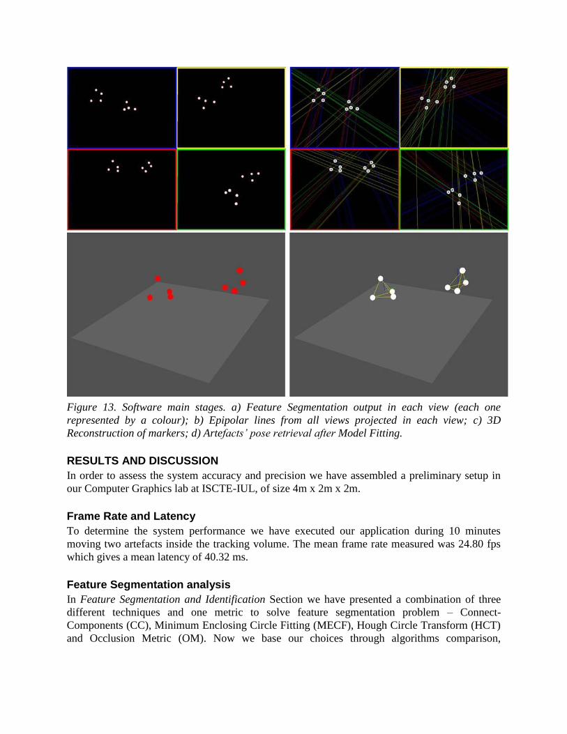
Figure 13. Software main stages. a) Feature Segmentation output in each view (each one

represented by a colour); b) Epipolar lines from all views projected in each view; c) 3D

Reconstruction of markers; d) Artefacts’ pose retrieval after Model Fitting.

RESULTS AND DISCUSSION

In order to assess the system accuracy and precision we have assembled a preliminary setup in

our Computer Graphics lab at ISCTE-IUL, of size 4m x 2m x 2m.

Frame Rate and Latency

To determine the system performance we have executed our application during 10 minutes

moving two artefacts inside the tracking volume. The mean frame rate measured was 24.80 fps

which gives a mean latency of 40.32 ms.

Feature Segmentation analysis

In Feature Segmentation and Identification Section we have presented a combination of three

different techniques and one metric to solve feature segmentation problem – Connect-

Components (CC), Minimum Enclosing Circle Fitting (MECF), Hough Circle Transform (HCT)

and Occlusion Metric (OM). Now we base our choices through algorithms comparison,

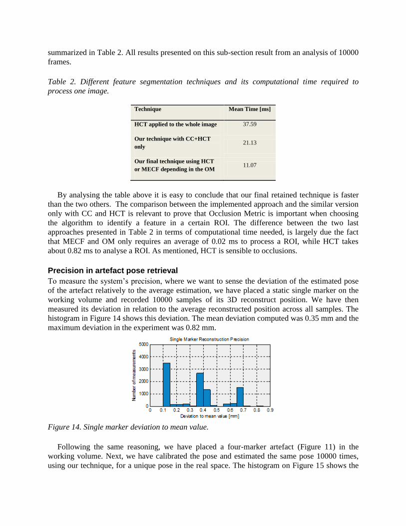
summarized in Table 2. All results presented on this sub-section result from an analysis of 10000

frames.

Table 2. Different feature segmentation techniques and its computational time required to

process one image.

Technique Mean Time [ms]

HCT applied to the whole image 37.59

Our technique with CC+HCT

only 21.13

Our final technique using HCT

or MECF depending in the OM 11.07

By analysing the table above it is easy to conclude that our final retained technique is faster

than the two others. The comparison between the implemented approach and the similar version

only with CC and HCT is relevant to prove that Occlusion Metric is important when choosing

the algorithm to identify a feature in a certain ROI. The difference between the two last

approaches presented in Table 2 in terms of computational time needed, is largely due the fact

that MECF and OM only requires an average of 0.02 ms to process a ROI, while HCT takes

about 0.82 ms to analyse a ROI. As mentioned, HCT is sensible to occlusions.

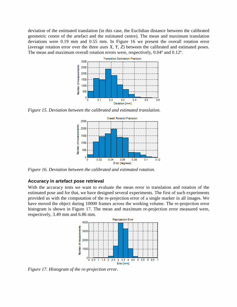
Precision in artefact pose retrieval

To measure the system’s precision, where we want to sense the deviation of the estimated pose

of the artefact relatively to the average estimation, we have placed a static single marker on the

working volume and recorded 10000 samples of its 3D reconstruct position. We have then

measured its deviation in relation to the average reconstructed position across all samples. The

histogram in Figure 14 shows this deviation. The mean deviation computed was 0.35 mm and the

maximum deviation in the experiment was 0.82 mm.

Figure 14. Single marker deviation to mean value.

Following the same reasoning, we have placed a four-marker artefact (Figure 11) in the

working volume. Next, we have calibrated the pose and estimated the same pose 10000 times,

using our technique, for a unique pose in the real space. The histogram on Figure 15 shows the

deviation of the estimated translation (in this case, the Euclidian distance between the calibrated

geometric centre of the artefact and the estimated centre). The mean and maximum translation

deviations were 0.19 mm and 0.55 mm. In Figure 16 we present the overall rotation error

(average rotation error over the three axes X, Y, Z) between the calibrated and estimated poses.

The mean and maximum overall rotation errors were, respectively, 0.04º and 0.12º.

Figure 15. Deviation between the calibrated and estimated translation.

Figure 16. Deviation between the calibrated and estimated rotation.

Accuracy in artefact pose retrieval

With the accuracy tests we want to evaluate the mean error in translation and rotation of the

estimated pose and for that, we have designed several experiments. The first of such experiments

provided us with the computation of the re-projection error of a single marker in all images. We

have moved the object during 10000 frames across the working volume. The re-projection error

histogram is shown in Figure 17. The mean and maximum re-projection error measured were,

respectively, 3.49 mm and 6.86 mm.

Figure 17. Histogram of the re-projection error.

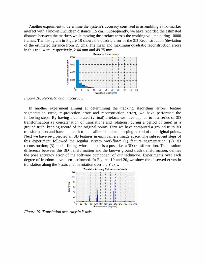
Another experiment to determine the system’s accuracy consisted in assembling a two-marker

artefact with a known Euclidean distance (15 cm). Subsequently, we have recorded the estimated

distance between the markers while moving the artefact across the working volume during 10000

frames. The histogram in Figure 18 shows the quadric error of the 3D Reconstruction (deviation

of the estimated distance from 15 cm). The mean and maximum quadratic reconstruction errors

in this trial were, respectively, 2.44 mm and 49.75 mm.

Figure 18. Reconstruction accuracy.

In another experiment aiming at determining the tracking algorithms errors (feature

segmentation error, re-projection error and reconstruction error), we have performed the

following steps. By having a calibrated (virtual) artefact, we have applied to it a series of 3D

transformations (a concatenation of translations and rotations, during a period of time) as a

ground truth, keeping record of the original points. First we have computed a ground truth 3D

transformation and have applied it to the calibrated points, keeping record of the original points.

Next we have re-projected all 3D features in each camera image space. The subsequent steps of

this experiment followed the regular system workflow: (1) feature segmentation; (2) 3D

reconstruction; (3) model fitting, whose output is a pose, i.e. a 3D transformation. The absolute

difference between this 3D transformation and the known ground truth transformation, defines

the pose accuracy error of the software component of our technique. Experiments over each

degree of freedom have been performed. In Figures 19 and 20, we show the observed errors in

translation along the Y axis and, in rotation over the Y axis.

Figure 19. Translation accuracy in Y axis.

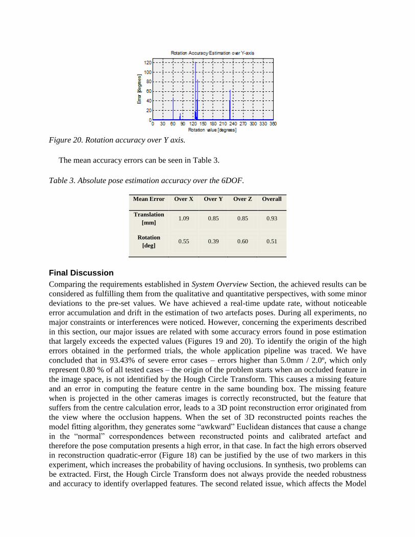
Figure 20. Rotation accuracy over Y axis.

The mean accuracy errors can be seen in Table 3.

Table 3. Absolute pose estimation accuracy over the 6DOF.

Mean Error Over X Over Y Over Z Overall

Translation

[mm] 1.09 0.85 0.85 0.93

Rotation

[deg] 0.55 0.39 0.60 0.51

Final Discussion

Comparing the requirements established in System Overview Section, the achieved results can be

considered as fulfilling them from the qualitative and quantitative perspectives, with some minor

deviations to the pre-set values. We have achieved a real-time update rate, without noticeable

error accumulation and drift in the estimation of two artefacts poses. During all experiments, no

major constraints or interferences were noticed. However, concerning the experiments described

in this section, our major issues are related with some accuracy errors found in pose estimation

that largely exceeds the expected values (Figures 19 and 20). To identify the origin of the high

errors obtained in the performed trials, the whole application pipeline was traced. We have

concluded that in 93.43% of severe error cases – errors higher than 5.0mm / 2.0º, which only

represent 0.80 % of all tested cases – the origin of the problem starts when an occluded feature in

the image space, is not identified by the Hough Circle Transform. This causes a missing feature

and an error in computing the feature centre in the same bounding box. The missing feature

when is projected in the other cameras images is correctly reconstructed, but the feature that

suffers from the centre calculation error, leads to a 3D point reconstruction error originated from

the view where the occlusion happens. When the set of 3D reconstructed points reaches the

model fitting algorithm, they generates some “awkward” Euclidean distances that cause a change

in the “normal” correspondences between reconstructed points and calibrated artefact and

therefore the pose computation presents a high error, in that case. In fact the high errors observed

in reconstruction quadratic-error (Figure 18) can be justified by the use of two markers in this

experiment, which increases the probability of having occlusions. In synthesis, two problems can

be extracted. First, the Hough Circle Transform does not always provide the needed robustness

and accuracy to identify overlapped features. The second related issue, which affects the Model

Fitting correspondence, relates to our manual and error-prone artefact construction and design,

which does not maximize the minimum Euclidean distance between artefact markers. Both

problems will be addressed in the following chapter.

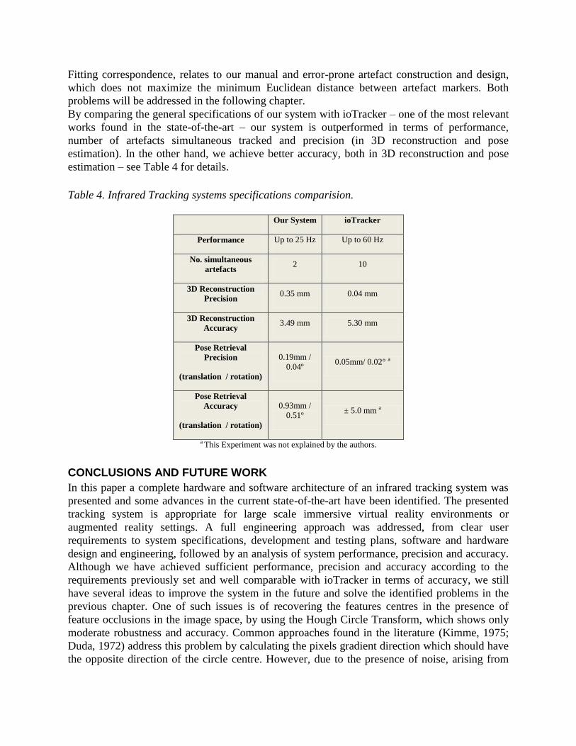
By comparing the general specifications of our system with ioTracker – one of the most relevant

works found in the state-of-the-art – our system is outperformed in terms of performance,

number of artefacts simultaneous tracked and precision (in 3D reconstruction and pose

estimation). In the other hand, we achieve better accuracy, both in 3D reconstruction and pose

estimation – see Table 4 for details.

Table 4. Infrared Tracking systems specifications comparision.

Our System ioTracker

Performance Up to 25 Hz Up to 60 Hz

No. simultaneous

artefacts 2 10

3D Reconstruction

Precision 0.35 mm 0.04 mm

3D Reconstruction

Accuracy 3.49 mm 5.30 mm

Pose Retrieval

Precision

(translation / rotation)

0.19mm /

0.04º 0.05mm/ 0.02° a

Pose Retrieval

Accuracy

(translation / rotation)

0.93mm /

0.51º ± 5.0 mm a

a This Experiment was not explained by the authors.

CONCLUSIONS AND FUTURE WORK

In this paper a complete hardware and software architecture of an infrared tracking system was

presented and some advances in the current state-of-the-art have been identified. The presented

tracking system is appropriate for large scale immersive virtual reality environments or

augmented reality settings. A full engineering approach was addressed, from clear user

requirements to system specifications, development and testing plans, software and hardware

design and engineering, followed by an analysis of system performance, precision and accuracy.

Although we have achieved sufficient performance, precision and accuracy according to the

requirements previously set and well comparable with ioTracker in terms of accuracy, we still

have several ideas to improve the system in the future and solve the identified problems in the

previous chapter. One of such issues is of recovering the features centres in the presence of

feature occlusions in the image space, by using the Hough Circle Transform, which shows only

moderate robustness and accuracy. Common approaches found in the literature (Kimme, 1975;

Duda, 1972) address this problem by calculating the pixels gradient direction which should have

the opposite direction of the circle centre. However, due to the presence of noise, arising from

the image acquisition and from markers prone-error manufacturing, these approaches tend to

compromise the robustness. On the other hand, techniques that fit 2D data points in geometric

shapes (e.g. a circle), have shown better accuracy and speed. One of the future research

directions to address this problem is the topic of data fitting applicable to feature occlusion cases.

Recent scientific contributions have shown the effectiveness of maximum likelihood estimation

to fit a cloud of 2D points with occlusions, in several circles (Frosio, 2008). Another alternative

way to develop the feature detection is through hardware segmentation. The CCD cameras allow

us to regulate the light that enters through the camera lens or to change the exposure time. These

two changes usually create a detectable gradient between two features that were previously

occluded, avoiding the utilization of the costly Hough Circle Transform. However, the artefacts’

support infrastructure should be made of a material that should not reflect light, and should

ideally be transparent and rigid to support the markers, or otherwise would create even more

unpredictable occlusions. We would need to find or create such material, with the aid of a

Materials Engineering Department of a well ranked University. A parallel approach is the

introduction of predicting filters, such as the Kalman Filter (Welch, 2004), to perform

comparisons between estimated and predicted poses and develop heuristics to choose the best fit,

in order to minimize the pose error. Additionally, by analysing the pose changes between frames,

cut-off translations and rotations could be defined, since there is certainly a change limit for both

transformations, in a time interval of 40 ms (25 Hz) which corresponds to the time between two

frames. Another envisaged improvement is a better artefact design based on topology

assessment. Our lab-made artefacts do not have the sub-millimetre precision required to enhance

the model fitting complexity reduction, which force us to have an off-line artefact calibration

phase. We hope to achieve a precise artefact construction which will allow us to suppress the

artefact calibration phase and introduce artefacts in the system only by its geometric and

topological description. Approaches to design artefacts that maximize the minimal Euclidean

distance across all markers (Pintaric, 2008) are foreseen and for that, collaboration with the

Architecture department of ISCTE-IUL is envisaged. By reducing the size of markers, which

reduce the probability of occlusion, we could improve the features detection. Alternatively, we

could combine information from several cameras. This is especially beneficial when, in a certain

view a feature is occluded and, in another view, the same feature is detected only through the

pixel-connected algorithm. This information could be correlated in the Multiple View

Correlation phase and used to solve the feature segmentation problem in a robust way. We also

plan to investigate the applicability of GPU computing and advanced parallel programming in

our system, namely in algorithms with no interwork dependences (e.g., Feature Segmentation,

Candidate Evaluation) which could benefit from the number of pipelines available in modern

GPUs. There are several examples in literature of faster implementations in GPU than CPU

(Yang, 2002; Moreland, 2003). Moreover, each module develop in our system can be applied in

several fields. The feature identification algorithm can be integrated in any problem that needs to

identify circular primitives (e.g. medical imaging). Any problem regarding 3D reconstruct of

world point from several views can use our approach of Multiple View Correlation. Examples of

such problems can be found in object tracking for augmented reality, 3D object and scene

reconstruction for SLAM (Simultaneous Localization and Mapping) in robotics, general 3D

scene reconstruction and mapping or image stitching.

ACKNOWLEDGMENTS

We would like to thank Rui Varela and Pedro Martins, of ISCTE-IUL for designing and

developing the system’s electronics and to thank Luciano Pereira Soares of PUC Rio de Janeiro

and Petrobrás for the lens model simulation.

REFERENCES

Abdel-Aziz, Y. I. & Karara, H. M. (1971). Direct Linear Transformation into Object Space

Coordinates in Close-Range Photogrammetry. In Procedures of Symposium of Close-Range

Photogrammetry. (pp. 1-18).

ART. (2011). Advanced Realtime Tracking GmbH. Retrieved July 5, 2011, from: http://www.ar-

tracking.de

Arun, K. S., Huang, T. S. & Blostein, S. D. (1987). Least-squares fitting of two 3-D point sets. In

IEEE Transactions on Pattern Analysis and Machine Intelligence. (pp. 698-700).

AVT. (2011). Allied Vision Technologies. Retrieved July 5, 2011, from:

http://www.alliedvisiontec.com

Cruz-Neira, C., Sandin, D., DeFanti, T., Kenyon, R. & Hart J. (1992). The CAVE: Audio Visual

Experience Automatic Virtual Environment. In Communications of the ACM: Vol. 35. (pp. 72-

65).

DeMenthon, D. & Davis, L. S. (1992). Model-Based Object Pose in 25 Lines of Code. In

European Conference on Computer Vision. (pp. 335-343).

Dias, J. M. S. & Bastos, R. (2006). An Optimized Marker Tracking System. In 12th

Eurographics Symposium on Virtual Environments. (pp. 1-4).

Dias, J. M. S. & et al. (2007). CAVE-HOLLOWSPACE do Lousal – Príncipios Teóricos e

Desenvolvimento. In Encontro Português de Computação Gráfica 15.

Dias, J. M. S., Jamal, N., Silva, P. & Bastos, R. (2004). ARTIC: Augmented Reality Tangible

Interface by Colour Evaluation. In Interacção 2004.

Duda, R. O. & Hart, P. E. (1972). Use of the Hough transformation to detect lines and curves in

pictures. In Communications of the Association for Computing Machinery: Vol 15. (pp. 11–15).

Fitzgibbon, A. W. & Fisher, R. B. (1995). A buyer’s guide to conic fitting. In Proceedings of the

5th British Machine Vision Conference: Vol 5. (pp. 513-522).

Frosio, I. & Borghese, N. A. (2008). Real-time accurate circle fitting with occlusions.

International Journal of Pattern Recognition, 41(3), 1041-1055.

Golub, G. H. & Van Loan, C. F. (1993). Matrix Computations. Baltimore. Maryland: Johns

Hopkins University Press.

Haralick, R. M., Joo, H., Lee, C. N., Zhuang, X., Vaidya, V.G. & Kim, M. B. (1989). Pose

estimation from corresponding point data. In IEEE Transactions on In Systems, Man, and

Cybernetics: Vol 19. (pp. 1426-1446).

Hartley, R. & Zisserman, A. (2003). Multiple View Geometry in Computer Vision. Cambridge:

Cambridge University Press.

Heikkila, J. & Silven, O. (1997). A Four-step Camera Calibration Procedure with Implicit Image

Correction. In Proceedings of the 1997 Conference on Computer Vision and Pattern

Recognition. (pp. 1106-1112).

Kato, H. & Billinghurst, M. (1999). Marker Tracking and HMD Calibration for a Video-Based

Augmented Reality Conferencing System. In Proceedings of the 2nd IEEE and ACM

International Workshop on Augmented Reality.

Kimme, C., Ballard, D. H. & Sklansky, J. (1975). Finding circles by an array of accumulators. In

Communications of the Association for Computing Machinery: Vol 18. (pp. 120-122).

Konc, J. & Janežiči, D. (2007). An improved branch and bound algorithm for the maximum

clique problem. In MATCH Communications in Mathematical and in Computer Chemistry: Vol

58. (pp. 569-590).

Lowe, D. G. (1991). Fitting Parameterized Three-Dimensional Models to Images. In IEEE

Transactions on Pattern Analysis and Machine Intelligence: Vol 13. (pp. 441-450).

Moreland, K. & Angel, E. (2003). The FFT on a GPU. In SIGGRAPH/Eurographics Workshop

on Graphics Hardware 2003 Proceedings. (pp. 112-119).

NI. (2011). National Instruments. Retrieved July 5, 2011, from: http://www.ni.com/

OpenCV. (2011). Open Computer Vision Library. Retrieved July 5, 2011, from:

http://sourceforge.net/projects/opencvlibrary/

Pintaric, T. & Kaufmann, H. (2007). Affordable Infrared-Optical Pose-Tracking for Virtual and

Augmented Reality. In Proceedings of Trends and Issues in Tracking for Virtual Environments

Workshop.

Pintaric, T. & Kaufmann, H. (2008). A Rigid-Body Target Design Methodology for Optical Pose

Tracking Systems. In Proceedings of the 15th ACM Symposium on Virtual Reality Software and

Technology. (pp. 73-76).

Santos, P., Buanes, A. & Jorge, J. (2006). PTrack: Introducing a Novel Iterative Geometric Pose

Estimation for a Marker-based Single Camera Tracking System. In IEEE Virtual Reality

Conference. (pp. 143-150).

Santos, P., Stork, A., Buaes, A., Pereira, C. & Jorge, J. (2010). A real-time low-cost marker-

based multiple camera tracking solution for virtual reality applications. Journal of Real-Time

Image Processing, 5(2), 121-128.

Schneider. (2011). Schneider Kreuznach. Retrieved July 5, 2011, from:

http://www.schneiderkreuznach.com

Vicon. (2011). Motion Capture Systems from Vicon. Retrieved July 5, 2011, from:

http://www.vicon.com

Wang, F. (2004). A Simple and Analytical Procedure for Calibrating Extrinsic Camera

Parameters. In IEEE Transactions on Robotics and Automation: Vol 20. (pp. 121-124).

Welch, G. & Bishop, G. (2004). An Introduction to the Kalman Filter (Tech. Rep. No. 95-041).

Chapel Hill, NC, USA: University of North Carolina, Department of Computer Science.

Yang, R. & Welch, G. (2002). Fast image segmentation and smoothing using commodity

graphics hardware. Journal of Graphics Tools, 7(4), 91-100.

Zhang, Z. (1999). Flexible Camera Calibration by Viewing a Plane from Unknown Orientations.

In International Conference on Computer Vision: Vol 1. (pp. 666-673).

Zhao, J., Yan, D., Men. G & Zhang, Y. (2007). A method of calibrating intrinsic and extrinsic

camera parameters separately for multi-camera systems. In Proceedings of the Sixth

International Conference on Machine Learning and Cybernetics: Vol 3. (pp. 1548-1553).