Embed Size (px)
Citation preview
Accurate Non-Iterative O(n) Solution to the PnP Problem
CVLab - Ecole Polytechnique Fédérale de Lausanne
Francesc Moreno-NoguerVincent Lepetit
Pascal Fua
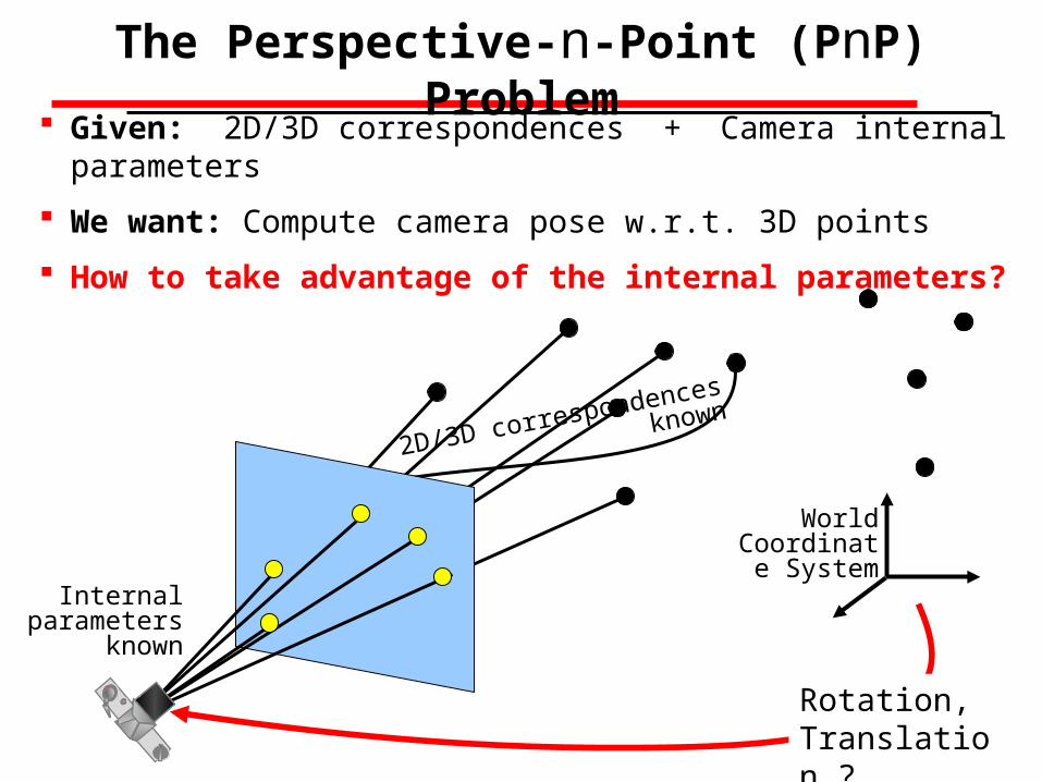
The Perspective-n-Point (PnP) Problem
Internal parameters
known
2D/3D correspondences known
Given: 2D/3D correspondences + Camera internal parameters
We want: Compute camera pose w.r.t. 3D points
How to take advantage of the internal parameters?
World Coordinate
System
Rotation, Translation ?

Church 1945
DeMenthon & Davis 1995
Dhome et al 1989
Haralick et al 1991
Horaud et al 1997
Kumar & Hanson 1994
Oberkampf et al 1996
Quan & Lan 1999
Gao et al 2003
Abbel & Karara 1971
Fischler & Bolles 1981
Horaud et al 1989
Lowe 1991
Triggs 1999
Ansar & Daniilidis 2003
Fiore 2001
Lu et al 2000
Scherighofer & Pinz 2006
Old Problem with many References
1940 1970 1980 1990 2000 2007
Church 1945
DeMenthon & Davis 1995
Dhome et al 1989
Haralick et al 1991
Horaud et al 1997
Kumar & Hanson 1994
Oberkampf et al 1996
Quan & Lan 1999
Gao et al 2003
Abbel & Karara 1971
Fischler & Bolles 1981
Horaud et al 1989
Lowe 1991
Triggs 1999
Ansar & Daniilidis 2003
Fiore 2001
Lu et al 2000
Scherighofer & Pinz 2006
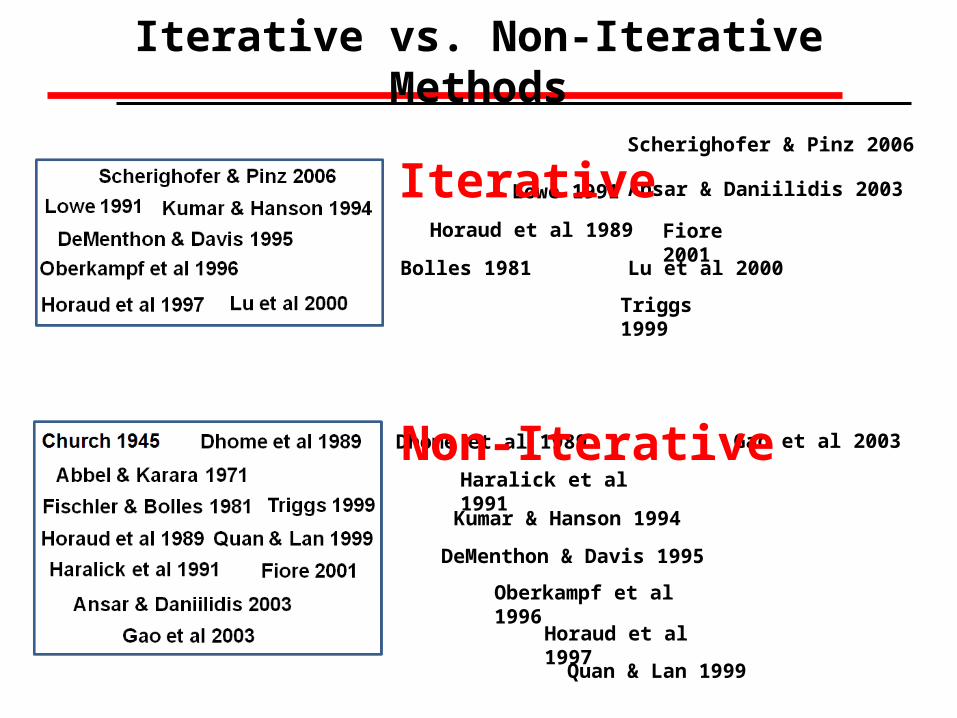
Iterative vs. Non-Iterative Methods
Iterative
Non-Iterative
Non-Iterative
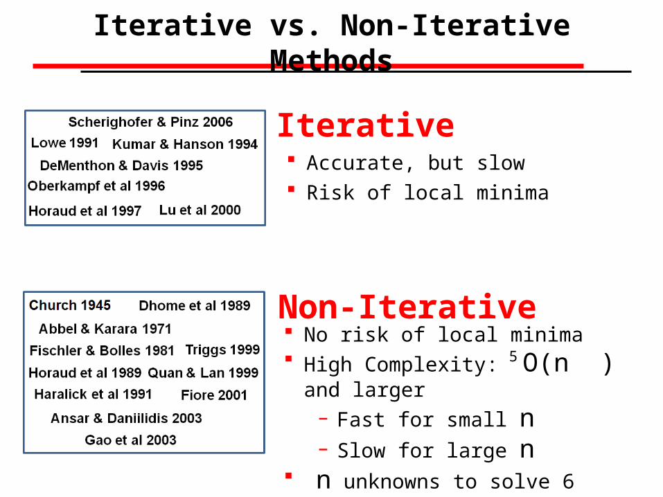
Iterative vs. Non-Iterative Methods
Iterative Accurate, but slow Risk of local minima
No risk of local minima High Complexity: O(n ) and larger
– Fast for small n– Slow for large n
n unknowns to solve 6 DoF !!!!
5
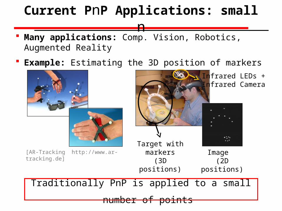
Current PnP Applications: small n
Many applications: Comp. Vision, Robotics, Augmented Reality
Example: Estimating the 3D position of markers
[AR-Tracking http://www.ar-tracking.de] Image (2D positions)
Infrared LEDs +Infrared Camera
Traditionally PnP is applied to a small number of points
Target with markers
(3D positions)
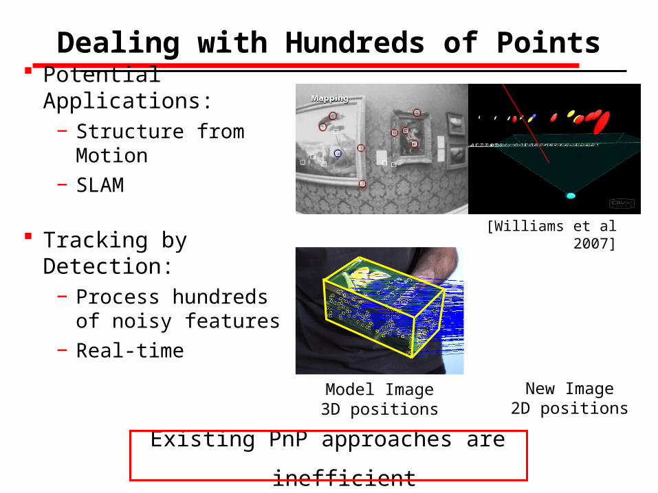
Dealing with Hundreds of Points
Tracking by Detection: − Process hundreds of
noisy features
− Real-time
Existing PnP approaches are inefficient
Model Image3D positions
New Image2D positions
[Williams et al 2007]
Potential Applications: − Structure from Motion
− SLAM
EPnP: Efficient PnP
Fast:− Non-iterative algorithm: O(n)− Handle hundreds of points in real-time
Accurate− As accurate as iterative methods− Robust to noise
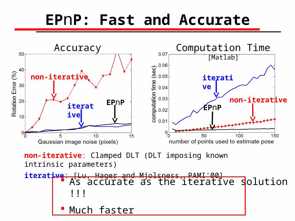
Computation Time [Matlab]
EPnP: Fast and Accurate
Accuracy
non-iterative: Clamped DLT (DLT imposing known intrinsic parameters)
iterative: [Lu, Hager and Mjolsness, PAMI'00]
EPnPiterative
non-iterative
As accurate as the iterative solution !!!
Much faster
iterative
EPnPnon-iterative
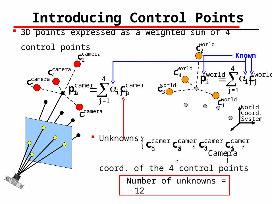
Unknowns:
Camera coord. of the 4 control points
World Coord. System
c 4world
c3world
c2world
c1world
c3camera
c4camera
c2camera
c1camera
Introducing Control Points
piworld
j=1
4
ijcjworld
picamera
j=1
4
ijcjcamera
Number of unknowns = 12
c1camera c2
camera c3camera c4
camera
3D points expressed as a weighted sum of 4 control points
Known
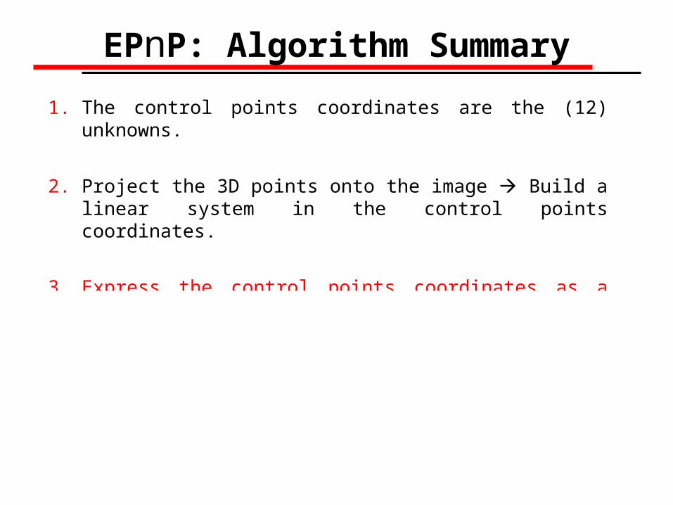
EPnP: Algorithm Summary
1. The control points coordinates are the (12) unknowns.
2. Project the 3D points onto the image Build a linear system in the control points coordinates.
3. The control points coordinates can be expressed as a linear combination of the null eigenvectors.
4. The weights ( the i ) are the new unknowns (not more than 4).
5. Adding rigidity constraints gives quadratic equations in the i .
6. Solving for the i depends on their number (linearization or relinearization).
c3camera
c4camera
c2camera
c1camera
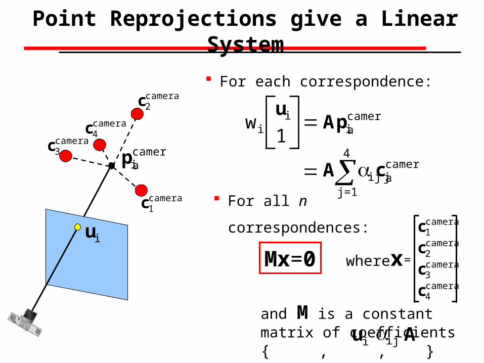
Point Reprojections give a Linear System
picamera
ui
ui
1wi pi
cameraA
j=1
4
ijcjcameraA
For each correspondence:
For all n correspondences:
Mx=0 where
c1camera
c2camera
c3camera
c4camera
x =
and M is a constant matrix of coefficients { , , }u i ij A
EPnP: Algorithm Summary
1. The control points coordinates are the (12) unknowns.
2. Project the 3D points onto the image Build a linear system in the control points coordinates.
3. The control points coordinates can be expressed as a linear combination of the null eigenvectors.
4. The weights ( the i ) are the new unknowns (not more than 4).
5. Adding rigidity constraints gives quadratic equations in the i .
6. Solving for the i depends on their number (linearization or relinearization).
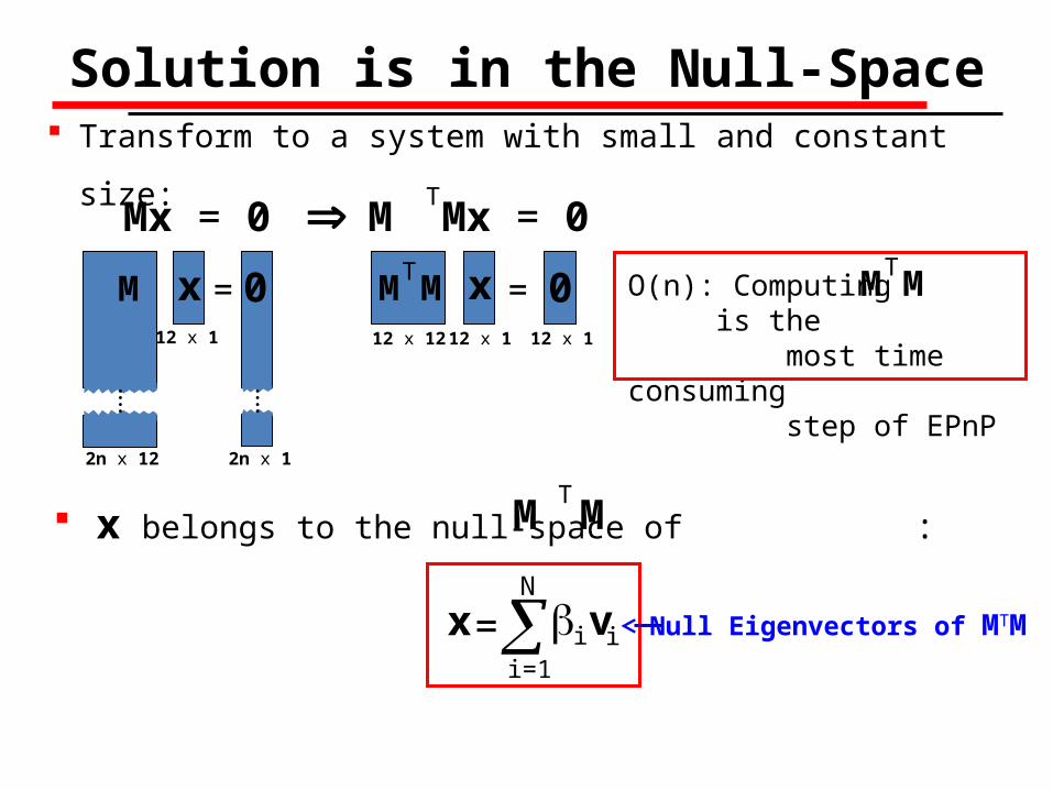
Transform to a system with small and constant size:
Solution is in the Null-Space
M Mx = 0T
Mx = 0
12 x 12
=12 x 1 12 x 1
x 0M MT O(n): Computing is the
most time consuming step of EPnP
M MT
x belongs to the null-space of :M TM
x =i=1
N
i vi
M
2n x 12
=12 x 1
2n x 1
x 0
Null Eigenvectors of MTM
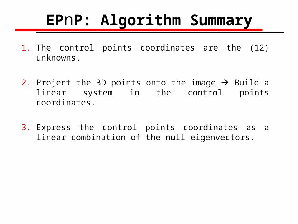
EPnP: Algorithm Summary
1. The control points coordinates are the (12) unknowns.
2. Project the 3D points onto the image Build a linear system in the control points coordinates.
3. Express the control points coordinates as a linear combination of the null eigenvectors.
4. The weights ( the i ) are the new unknowns (not more than 4).
5. Adding rigidity constraints gives quadratic equations in the i .
6. Solving for the i depends on their number (linearization or relinearization).

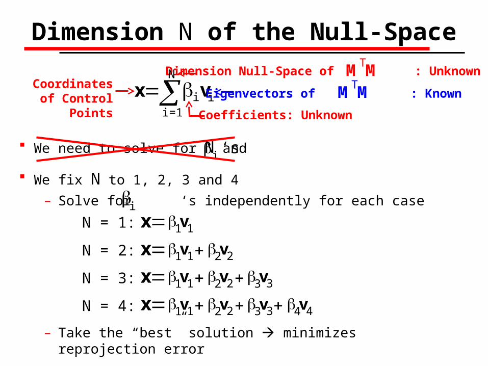
Dimension Null-Space of : UnknownM M T
We need to solve for N and
What is the dimension N of the null space of ?− Noise-Free Case: N=1
− In practice (noise):
No zero eigenvalues,
but several are small
Dimension N of the Null-Space
x i=1
N
i vi
Coefficients: Unknown
Coordinates of Control Points
M MT
‘si
Eigenvectors of : KnownM M T
We found that only the cases
N = 1, 2, 3 and 4 must be considered
62% N=1
28% N=2
9% N=31% N=4
Dimension Null-Space of : UnknownM M T
We need to solve for N and
Dimension N of the Null-Space
x i=1
N
i vi
Coefficients: Unknown
Coordinates of Control Points
‘si
Eigenvectors of : KnownM M T
We fix N to 1, 2, 3 and 4
– Solve for ‘s independently for each casei
1v1xN = 1:
1v1 2v2xN = 2:
1v1 2v2 3v3xN = 3:
1v1 2v2 3v3 4v4xN = 4:
– Take the “best” solution minimizes reprojection error
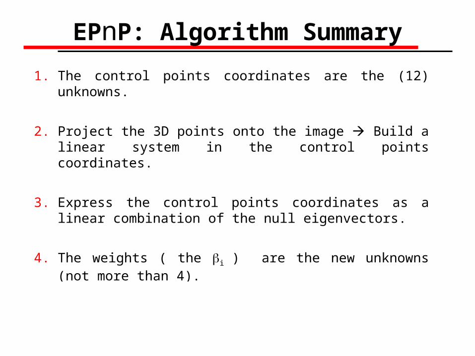
EPnP: Algorithm Summary
1. The control points coordinates are the (12) unknowns.
2. Project the 3D points onto the image Build a linear system in the control points coordinates.
3. Express the control points coordinates as a linear combination of the null eigenvectors.
4. The weights ( the i ) are the new unknowns (not more than 4).
5. Adding rigidity constraints gives quadratic equations in the i .
6. Solving for the i depends on their number (linearization or relinearization).
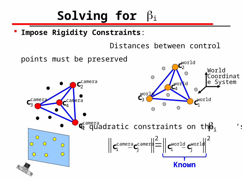
Impose Rigidity Constraints:
Distances between control points must be preserved
c4world
c2world
c3world
c1world
Solving for i
cjworldci
world2
cicamera cj
camera2
6 quadratic constraints on the ‘s :i
Known
c1camera
c4camerac3
camera
c2camera
World Coordinate System
EPnP: Algorithm Summary
1. The control points coordinates are the (12) unknowns.
2. Project the 3D points onto the image Build a linear system in the control points coordinates.
3. Express the control points coordinates as a linear combination of the null eigenvectors.
4. The weights ( the i ) are the new unknowns (not more than 4).
5. Add rigidity constraints to get quadratic equations in the i .
6. Solving for the i depends on their number (linearization or relinearization).
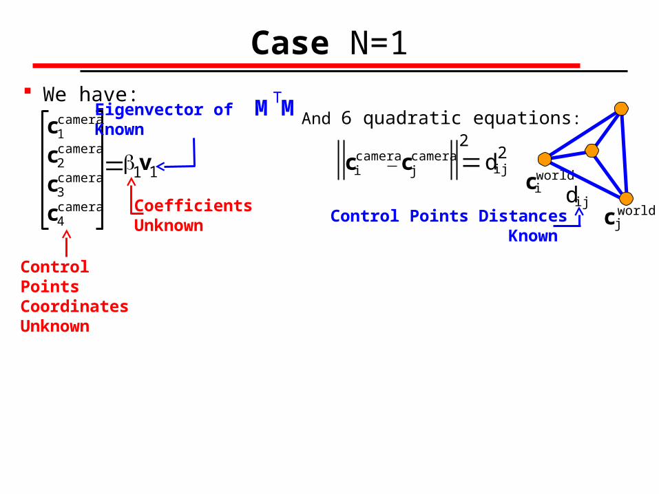
Case N=1 We have:
ciworld
c jworld
dij
2And 6 quadratic equations:
cicamera cj
camera 2dij
c1camera
c2camera
c3camera
c4camera
1v1
Control Points DistancesKnown
Control Points CoordinatesUnknown
Eigenvector of Known
M M T
CoefficientsUnknown
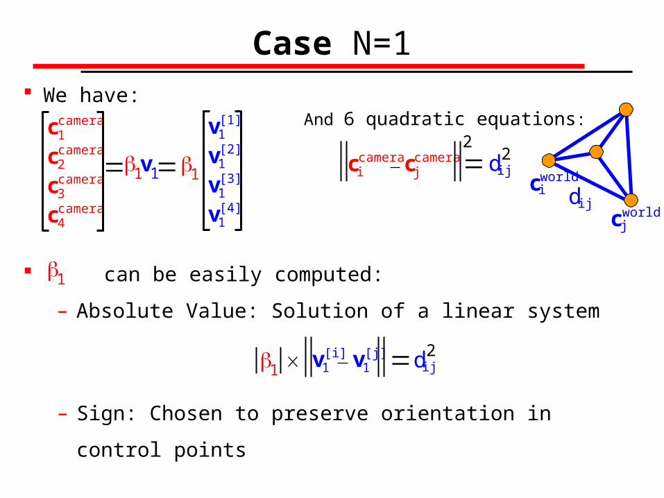
Case N=1
2And 6 quadratic equations:
cjworld
d ij
We have:
can be easily computed:
– Absolute Value: Solution of a linear system
1
1
v1[1]
v1[2]
v1[3]
v1[4]
1 v1[i] v1
[j] 2dij
– Sign: Chosen to preserve orientation in control points
cicamera cj
camera 2dij
c1camera
c2camera
c3camera
c4camera
1v1 ciworld
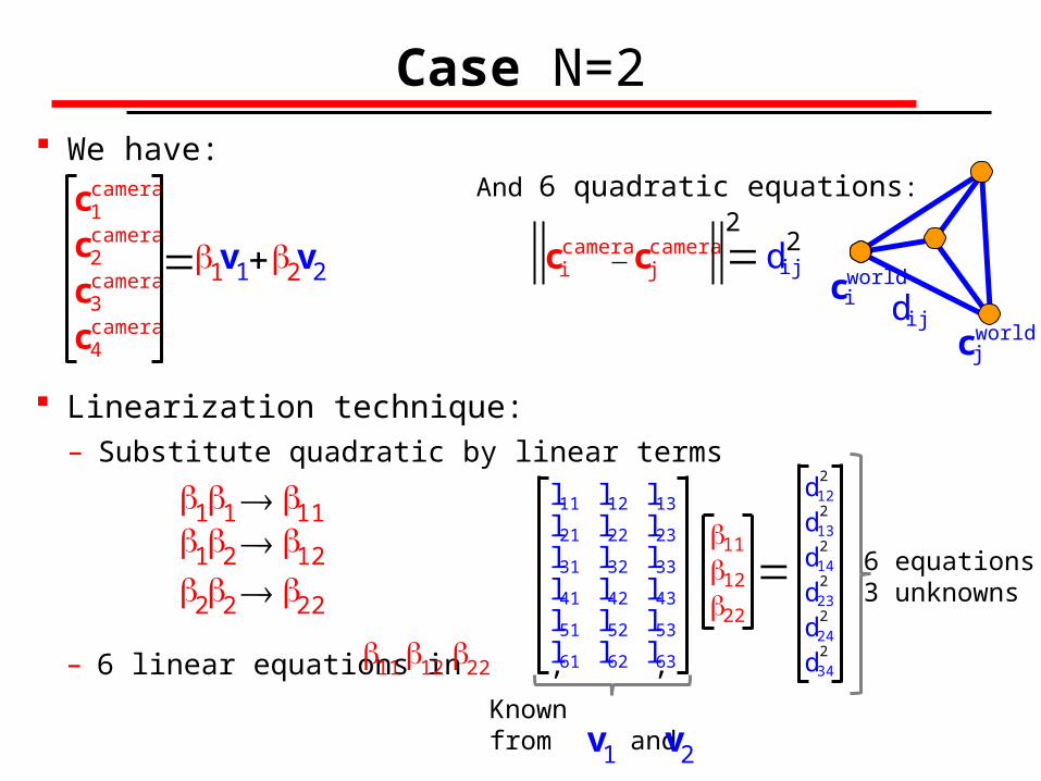
Case N=2
2And 6 quadratic equations:
cjworld
d ij
We have:
Linearization technique:– Substitute quadratic by linear terms
– 6 linear equations in , ,
11 1112 1222 22
11 12 22
6 equations3 unknowns
cicamera cj
camera 2dij
c1camera
c2camera
c3camera
c4camera
1v1 2v2
Knownfrom and v2v1
l13
l23
l33
l43
l53
l63
l11
l21
l31
l41
l51
l61
l12
l22
l32
l42
l52
l62
11
12
22
d122
d132
d142
d232
d242
d342
ciworld
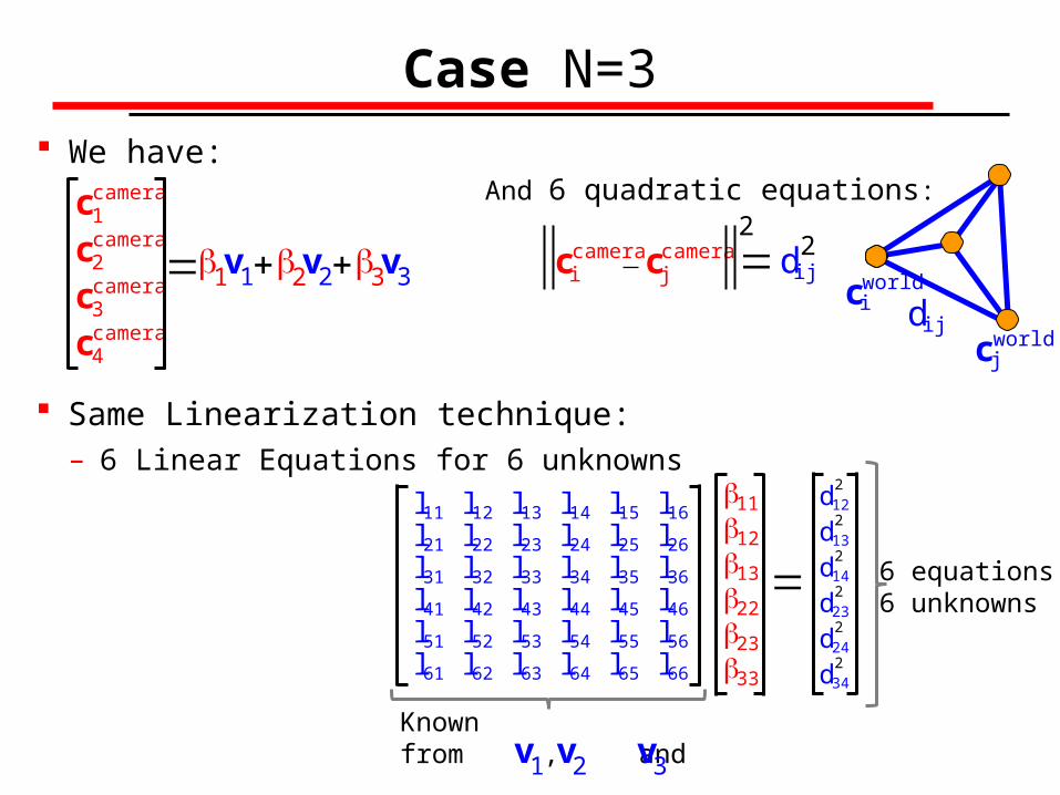
Case N=3
2c1
camera
c2camera
c3camera
c4camera
And 6 quadratic equations:
cicamera cj
camera 2dij
cjworld
d ij
We have:
Same Linearization technique:– 6 Linear Equations for 6 unknowns
1v1 2v2 3v3
Knownfrom , and v2v1 v3
l16
l26
l36
l46
l56
l66
l14
l24
l34
l44
l54
l64
l15
l25
l35
l45
l55
l65
d122
d132
d142
d232
d242
d342
6 equations6 unknowns
l13
l23
l33
l43
l53
l63
l11
l21
l31
l41
l51
l61
l12
l22
l32
l42
l52
l62
11
12
13
22
23
33
ciworld
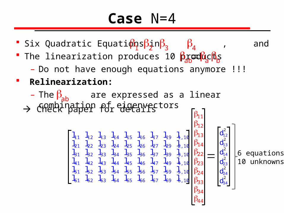
Case N=4
Six Quadratic Equations in , , and The linearization produces 10 products
– Do not have enough equations anymore !!! Relinearization:
– The are expressed as a linear combination of eigenvectors
ab
a
b
1
2
3
4
ab
Check paper for details
6 equations10 unknowns
11
12
13
14
22
23
24
33
34
44
l1,10
l2,10
l3,10
l4,10
l5,10
l6,10
l17
l27
l37
l47
l57
l67
l19
l29
l39
l49
l59
l69
l16
l26
l36
l46
l56
l66
l54
l14
l24
l34
l44
l64
l15
l25
l35
l45
l55
l65
l13
l23
l33
l43
l53
l63
l51
l11
l21
l31
l41
l61
l12
l22
l32
l42
l52
l62
d122
d132
d142
d232
d242
d342

EPnP: Algorithm Summary
1. The control points coordinates are the (12) unknowns.
2. Project the 3D points onto the image Build a linear system in the control points coordinates.
3. Express the control points coordinates as a linear combination of the null eigenvectors.
4. The weights ( the i ) are the new unknowns (not more than 4).
5. Add rigidity constraints to get quadratic equations in the i .
6. Solve for the i depending on their number (linearization or relinearization).
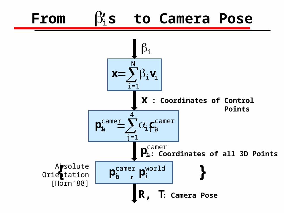
From ‘s to Camera Pose
: Coordinates of Control Points
x i=1
N
i vi
x
picamera
j=1
4
ijcjcamera
picamera
: Coordinates of all 3D Points
i
i
{ , } picamera pi
world
: Camera PoseR, T
Absolute Orientation
[Horn’88]
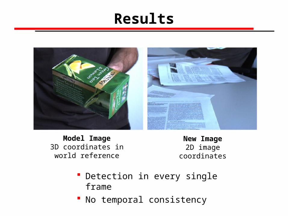
Results
Detection in every single frame No temporal consistency
Model Image3D coordinates in world
reference
New Image2D image coordinates
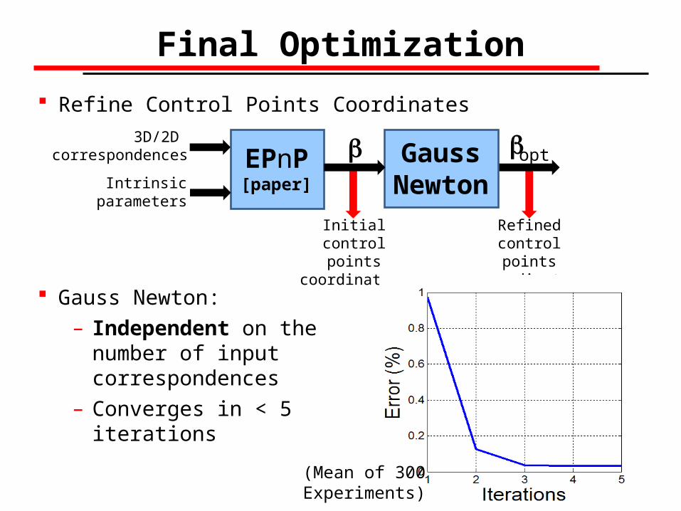
Final Optimization
Refine Control Points Coordinates
EPnP
Refined control points coordinates
Gauss Newton:
– Independent on the number of input correspondences
– Converges in < 5 iterations
3D/2D correspondences
Intrinsic parameters
Initialcontrol points coordinates
optGauss Newton
(Mean of 300 Experiments)
[paper]
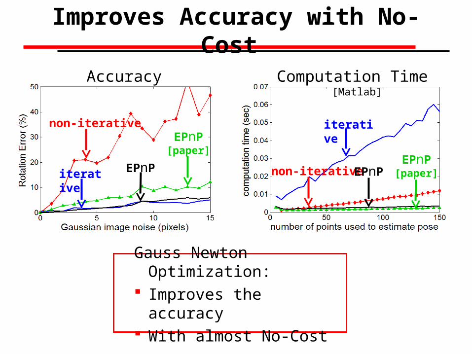
Improves Accuracy with No-Cost
Gauss Newton Optimization: Improves the accuracy With almost No-Cost
EPnP
non-iterative
iterative non-iterative
iterative
EPnP
EPnP[paper]
EPnP[paper]
Computation Time [Matlab]Accuracy
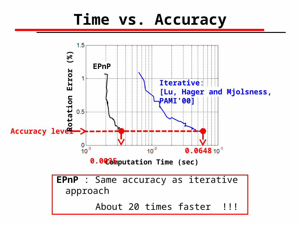
Time vs. Accuracy
Accuracy level
EPnPR
ota
tio
n E
rro
r (%
)
Computation Time (sec)
EPnP : Same accuracy as iterative approach
About 20 times faster !!!
Iterative: [Lu, Hager and Mjolsness, PAMI'00]
0.0035 0.0648

Conclusions & Future Work
O(n) non-iterative solution to the PnP problem– As accurate as iterative methods
– Much faster
Simple central idea: – Represent 3D coordinates as a weighted sum of 4 control points
– Potentially applicable to other problems– Structure from Motion– Deformable surfaces

Code Available:
http://cvlab.epfl.ch/~fmoreno/Publications/ICCV07
Thanks !!