Embed Size (px)
Citation preview

ACE: Abstracting, Characterizing and Exploiting
Peaks and Valleys in Datacenter Power
Consumption
Di Wang∗,
Chuangang Ren∗,
Sriram Govindan†,
Anand Sivasubramaniam∗,
Bhuvan Urgaonkar∗,
Aman Kansal‡,
Kushagra Vaid†
∗Department of Computer Science and Engineering,∗The Pennsylvania State University
†Microsoft‡Microsoft Research
Technical Report. CSE 13-003.
May 2, 2013
1
Abstract
Peak power management of datacenters has tremendous cost impli-cations. While numerous mechanisms have been proposed to cap powerconsumption, real datacenter power consumption data is scarce. Priorstudies have either used a small set of applications and/or servers, orpresented data that is at an aggregate scale from which it is difficult todesign and evaluate new and existing optimizations. To address thisgap, we collect power demands at multiple spatial and fine-grainedtemporal resolutions from the load of geo-distributed datacenters ofMicrosoft over 6 months. We conduct aggregate analysis of this data,to study its statistical properties. We find evidence of self-similarity inpower demands, statistical multiplexing suggesting tighter provision-ing at higher levels in the power hierarchy, and correlations with thecooling power that caters to the IT equipment.
With workload characterization a key ingredient for systems de-sign and evaluation, we note the importance of better abstractions forcapturing power demands, in the form of peaks and valleys. We iden-tify attributes for peaks and valleys, and important correlations acrossthese attributes that can influence the choice and effectiveness of dif-ferent power capping techniques. We characterize these attributes andtheir correlations, showing the burstiness of small duration peaks, andthe importance of not ignoring the rare but more stringent/long peaks.The correlations between peaks and valleys, also suggest the need fortechniques to aggregate and collectively handle them. With the widescope of exploitability of such characteristics for power provisioning andoptimizations, we illustrate its benefits with two specific case stud-ies. The first shows how peaks can be differentially handled based onour peak and valley characterization using existing approaches, ratherthan a one-size-fits-all solution. The second illustrates a simple ca-pacity provisioning strategy for energy storage, using the peak andvalley characteristics, that can suppress 99.9% of the peaks and 90%of the area under the peaks, at a capacity which is less than half of theoptimal that is designed to address every eventuality.
1 Introduction
The cost, scalability and environmental concerns arising from the powerconsumption of datacenters has come under extensive scrutiny. While muchof the prior work in the area has looked to reduce energy of computing andcooling systems, the importance of how this energy is dissipated over time(i.e. the power) has gained a lot of recent attention. Power dissipation,particularly the peak or high power draws, impact both operational (op-ex)and capital (cap-ex) expenditures. Electric utilities can charge differentially(op-ex) for peaks (e.g. [9]), especially if such high power draws coincide withhigh demand across the grid because of supply-demand mismatches thatcan lead to potential black or brown-outs. Peak power draws also determinethe capacity of the power distribution and cooling infrastructure that is
2

provisioned within the datacenter. Prior studies [12, 24] have pointed outthat provisioning costs can range between $10-20 per watt, which is incurredeven if that watt is not actually consumed.
To address this problem, numerous prior optimizations have been pro-posed. However, there is a lack of real world datacenter power consumptiondata to guide the design and enable thorough evaluation of these optimiza-tions. Detailed power consumption data at different temporal scales (fromseconds to months) and spatial granularities (from servers, chassis, racks, todatacenters) for datacenters serving important workloads is not easily avail-able. This paper intends to fill this critical void by providing an in-depthanalysis of measured power characteristics from the datacenter infrastruc-ture of Microsoft corporation.Power Characterization: Workload characterization is a key ingredientto the design and analysis of any system that is intended to cater to thisworkload. It can provide important guidelines regarding how to design thesystem to handle the average, or a high percentile, of the workload. It alsoprovides the benchmarking ability to evaluate how a given system wouldperform. More importantly, it can help identify attributes of the workloadthat stress the system, quantify the statistical properties of these attributes,and exercise these properties in fine tuning and evaluating the system forthe future. Such a design can perform much better than one based on justa particular load or trace of the past. The statistical properties enable aneasier analysis to quickly examine performance behavior, system design andcapacity planning issues, etc., compared to a time consuming design andevaluation loop that may require access to the fine-resolution data over anextensive period of time (that may not necessarily be accessible to everyone).
Recognizing these benefits, there have been several prior efforts at work-load behavior or characterization for different system design issues, e.g. web,media and cloud services [1, 6, 18, 25, 27, 19], networking [32, 52], file andI/O systems [41, 23, 40], memory system errors [42], impact of datacentertemperature on failures [11], etc., and using these for different optimizations.
While one could take load characteristics and extrapolate them to powerdemands (using appropriate utilization to power translation models, e.g.[10, 4, 35, 12, 7, 26, 16, 43, 29]), there are several additional considerations:datacenters host multiple workloads and subsystems, with a complex set ofinteractions and correlations that could possibly exist across the workloadsor subsystems and it is not clear if the extrapolations would hold at theaggregate (temporal and spatial) level. Moreover, power modeling is still anactive area of research, with both linear and non-linear correlations betweenload or utilization and power being suggested [15, 12], and model accuracymay be insufficient for safety critical power capping operations. Instead,direct power measurement based characterization can avoid some of thesedeficiencies.Datacenter Power Characterization: Power measurement and charac-
3
terization, in most prior works, has typically used a few (datacenter) appli-cations and/or a few servers at best. For instance, observations of around20 servers in a production datacenter in [44] show under-utilization, withthe highest power peaks caused by virus scans. A study from IBM [45] ex-amined the temporal and spatial correlation of power consumption in smallclusters, each with about 20 servers. A similar characterization of MSNmessenger workload [17] has shown opportunities for better provisioning viaintelligent workload placement. The most notable large scale undertakingto study datacenter power demands from the provisioning perspective is thepublished effort from Google [12]. This study identified the headroom forover-provisioning IT equipment within the existing power infrastructure atdifferent spatial scales. The study was more intended to portray the poten-tial of power under-provisioning, rather than as a characterization effort forcapturing the statistical properties of the power demands, and their impacton the effectiveness of different power capping and/or power demand shap-ing knobs. As we will show, a more detailed abstraction (as in our peakand valley attributes) of the characteristics is necessary for these purposes,rather than an aggregate power demand represented as a simple CumulativeDensity Function.
To our knowledge, this is the first effort to undertake a systematic char-acterization of the power consumption of large computing infrastructures,that can be used for the design and evaluation of effective power demandshaping knobs. Such characterization may also be useful for datacenter en-ergy sourcing, including renewable options and geographical supply and/ordemand following [33, 8], though this is outside the scope of this paper.Power Capping/Demand Shaping: Broadly, there are three primarycategories of power capping knobs - we will consider demand shaping mainlyfrom the perspective of power capping in this paper, which as noted abovehas both cap-ex and op-ex benefits. Considering the power distribution net-work as a hierarchy flowing from incoming utility lines, to step-down trans-formers, UPS units, and Power Distributions Units, that subsequently feedto chassis and racks, and finally to individual outlets for each server, powercapping knobs can be employed at one or more of these levels in the hier-archy.Temporal knobs include load scheduling or deferral, which temporallymove portions of the load from peaks to valleys to shave the former. Thesemay be implemented through dynamic voltage-frequency scaling (DVFS)techniques that slow down the execution, admission control techniques thatdrop load during peak demand, or by delaying execution to a low demandtime (valleys) [34, 38, 48, 15, 50, 14, 36, 43, 2, 46, 3, 51]. Spatial knobsleverage heterogeneity of power demands at any time across the datacen-ter, and either statistically multiplexing their low probability simultaneousoccurrence to co-locate them within a level [39, 20, 37, 49, 13, 31, 12, 17]or migrate workloads to regions in the hierarchy with headroom (valleys)from regions that are operating at their peak [20, 17, 30, 5, 3]. A recent set
4

of knobs leverages energy storage devices (ESDs), such as batteries, ultra-capacitors, etc., to provide just-in-time extra capacity for the power peaksby hoarding the required capacity (energy) in previous valleys (when de-mand was lower) [21, 22, 28, 47]. Depending on where they are placed inthe power distribution hierarchy, ESDs can suppress peaks from propagatinghigher up in the hierarchy.Overview: In general, the efficacy of all these power capping knobs dependson the peak and valley characteristics of power draws in the power hierarchy.For example, temporal deferrals require subsequent valleys large enough tospill over the work from a previous peak. Spatial migration or multiplexingrequires a valley elsewhere in the hierarchy to overlap with a peak to besuppressed. ESDs require sufficient valleys, either in number or magnitude,to have sufficient slack to re-charge their capacity preceding the peak thatit has to suppress, etc. Consequently, while we do present statistics ofaggregate power demands at different temporal and spatial scales (in section2), we focus more detailed characterization results on peaks and valleysin these demands (in section 4), after formally defining these terms for aspecified level of power capping in section 3.Contributions: We collected fine-grained power traces from multiple serverclusters, each comprising hundreds of servers spanning multiple chassis andracks, across several geo-distributed datacenters over a 6 month durationand make the following contributions:
• We present an aggregate power consumption analysis that shows howpower fluctuations change across different spatial and temporal scales.The analysis shows the effect of statistical multiplexing as we move fromfiner to coarser spatial scales, temporal dependence and self-similarity, andthe nature of correlation among server and cooling power consumptions.
• We formally define attributes for the peaks and valleys of power demandsfor a given power cap. These attributes - width (duration), height ordepth, and area (energy) - capture the stringency of the peaks (in powerand energy), and slack in the valleys.
• We extensively characterize these attributes individually for the peaksand valleys. We also quantify the cross-correlations between them, whichwould impact the effectiveness of different peak suppression knobs, e.g.ability of an ESD to re-charge and source its power before a given peak,the amount of work deferred by DVFS, etc.
• Our analysis shows that there are a large number of peaks of relativelyshort duration. These short duration peaks are also typically of small am-plitude (height), and occur in bursts. At the same time, we cannot ignorethe long duration peaks, which albeit occurring at lower frequencies, im-pose stringent demands on the peak suppression techniques. Our resultsalso suggest the possible need to look beyond the immediately successivepeak or valley, to perform better aggregate level optimizations, especially
5

for the smaller peaks.• While there are numerous use-cases of such characterization, we explore
two illustrative case-studies. The first exploits the properties of peakoccurrences and their stringency to differentially employ two peak sup-pression techniques (load deferral and spatial migration). The secondstudy uses information about peak attributes, and the valley opportuni-ties to come up with rough estimates for ESD technology and capacityprovisioning.
2 Aggregate Characteristics
In this section, we present a spatio-temporal analysis of power consump-tion, focusing on its aggregate characteristics. We illustrates the statisticalmultiplexing across multiple servers and racks, which results in a reducedmagnitude of power peaks at a coarser or more aggregate level. This re-affirms prior observations in [12], that deeper under-provisioning may beemployed higher up in the power hierarchy. On the temporal side, our re-sults show long range dependence in power demands, with strong evidenceof self-similarity.The auto-correlation analysis confirms the time-of-day be-havior in these demands. We also show how cooling power is correlated withserver power, and find that it not only lags server power by two minutes butalso has a higher variance.
2.1 Tracing and Data Collection
We collected power measurement data from multiple geo-distributed data-centers run by Microsoft over a six month period, between July-December2011. We specially give results here for data pertaining to 8 representativeserver clusters (see Table 1) in the interest of clarity. Each such clustercomprises several hundreds of servers that span multiple chassis and racks.These clusters run a variety of workloads including web-search, email, Map-Reduce jobs, and several other online cloud applications, catering to millionsof users around the world. Each cluster uses homogeneous hardware, thoughthere could be differences across clusters. We name the 8 clusters as C1, C2,..., C8 and present the trace collection resolution and the type (soft-realtime,batch and interactive) of application that each hosts in Table 1. Apart fromthe IT power of the clusters, we have also collected cooling power.
Cluster Names Data Resolution Application Type
C1, C2 20 seconds Soft-realtime, Batch
C3, C4, ..., C8 120 seconds Interactive
Table 1: Data collection is done for a period of six months. Each clusterhas several hundreds of servers
6
2.2 Statistical Properties
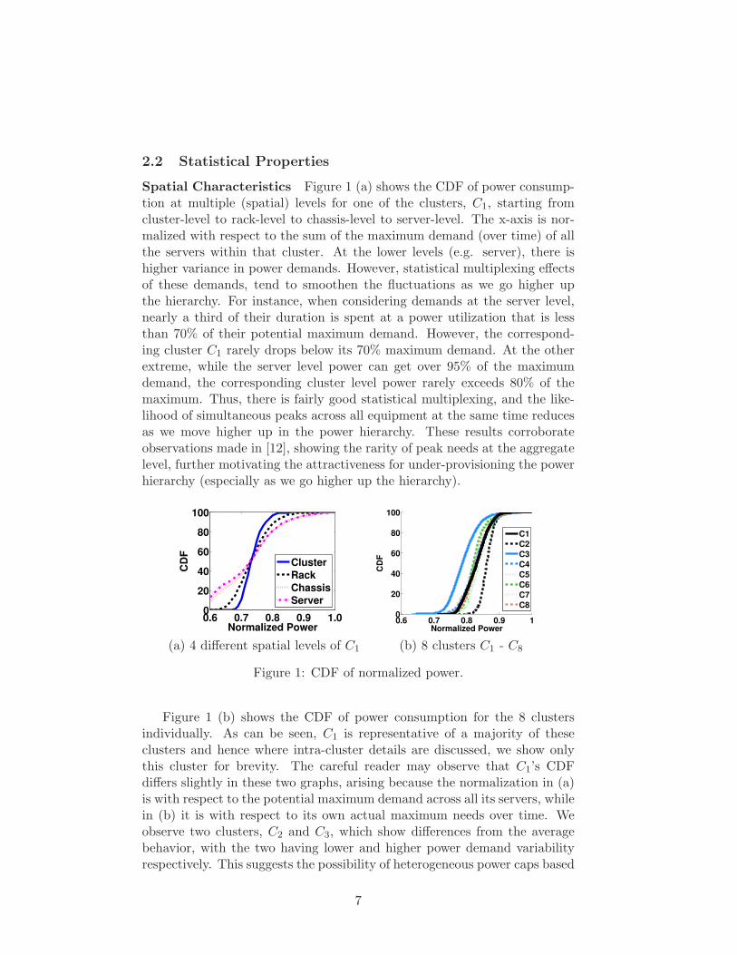
Spatial Characteristics Figure 1 (a) shows the CDF of power consump-tion at multiple (spatial) levels for one of the clusters, C1, starting fromcluster-level to rack-level to chassis-level to server-level. The x-axis is nor-malized with respect to the sum of the maximum demand (over time) of allthe servers within that cluster. At the lower levels (e.g. server), there ishigher variance in power demands. However, statistical multiplexing effectsof these demands, tend to smoothen the fluctuations as we go higher upthe hierarchy. For instance, when considering demands at the server level,nearly a third of their duration is spent at a power utilization that is lessthan 70% of their potential maximum demand. However, the correspond-ing cluster C1 rarely drops below its 70% maximum demand. At the otherextreme, while the server level power can get over 95% of the maximumdemand, the corresponding cluster level power rarely exceeds 80% of themaximum. Thus, there is fairly good statistical multiplexing, and the like-lihood of simultaneous peaks across all equipment at the same time reducesas we move higher up in the power hierarchy. These results corroborateobservations made in [12], showing the rarity of peak needs at the aggregatelevel, further motivating the attractiveness for under-provisioning the powerhierarchy (especially as we go higher up the hierarchy).
0.6 0.7 0.8 0.9 1.00
20
40
60
80
100
Normalized Power
CD
F
Cluster
Rack
Chassis
Server
0.6 0.7 0.8 0.9 10
20
40
60
80
100
CD
F
Normalized Power
C1
C2
C3
C4
C5
C6
C7
C8
(a) 4 different spatial levels of C1 (b) 8 clusters C1 - C8
Figure 1: CDF of normalized power.
Figure 1 (b) shows the CDF of power consumption for the 8 clustersindividually. As can be seen, C1 is representative of a majority of theseclusters and hence where intra-cluster details are discussed, we show onlythis cluster for brevity. The careful reader may observe that C1’s CDFdiffers slightly in these two graphs, arising because the normalization in (a)is with respect to the potential maximum demand across all its servers, whilein (b) it is with respect to its own actual maximum needs over time. Weobserve two clusters, C2 and C3, which show differences from the averagebehavior, with the two having lower and higher power demand variabilityrespectively. This suggests the possibility of heterogeneous power caps based
7

0 200 400 6000
0.5
1
Time (hour)
Auto
corr
ela
tion
0 200 400 6000
0.5
1
Time (hour)
Auto
corr
ela
tion
0 12 24 36 480.2
0.4
0.6
0.8
1
Time (hour)
Au
toco
rrela
tio
n
(a) Cluster C1 (b) Cluster C3 (c) Cluster C1 Zoomed-in
Figure 2: Auto correlation function for different time lags for clusters C1
and C3
on the workload. For instance, an 80% cap on C3 would impact it only 10%of the time, while such a cap would be unaccomplishable in the case of C2
(which probably can work only with a 90% cap). This suggests leveragingsuch heterogeneous caps in the datacenter to either dynamically imposethese restrictions, or mapping the workloads to appropriate regions of thepower hierarchy based on differential headrooms.
Temporal Characteristics One way to understand the temporal time se-ries of power demands is through an Auto-correlation Function (ACF) plotwith different time-lags. Figure 2 shows the ACFs for clusters C1 and C3.While there are some absolute value differences between the two clusters,the trends are similar, and we specifically focus on C1, and show a zoomed-in version of its ACF for time-lags stretching up to 48 hours (Figure 2 (c)).While there are significant near-term correlations in the time-series, we notethat there is a fairly good time-of-day behavior that is exhibited by the powerdemands - lags of 24 hours (and multiples) have high correlations, and lagsof 12 hours (and its odd number of multiples) are the least correlated. Fur-thermore, the slower than exponential decay of the ACF indicates that thedemands do not follow a Poisson process, with possibility of self-similarityover time. Self-similarity implies structural similarities across a wide rangeof time scales. To investigate the presence of self-similarity, we calculate theHurst parameter, using several techniques [18, 32, 52], including variance,R/S method, and periodogram plots. The results are consistent across thesetechniques. Hurst parameter is a measure of the level of self-similarity withvalue close to 1 indicating more self-similar. We find a high value for theHurst parameter, over 0.8, for all clusters (Figure 3), with the log-log vari-ance plot (Figure 5 (a)) and R/S method (Figure 5 (b)) specifically shownfor cluster C1. These quantitatively show the existence of self-similarity inthe power demands.
A visual examination of the time series, shown in Figure 4 at differenttime scales (20s to 2000s) of the average (normalized) power for C1, also gives
8

Cluster HurstName Parameter
C1 0.93
C2 0.91
C3 0.89
C4 0.90
C5 0.90
C6 0.82
C7 0.87
C8 0.86
Figure 3: Hurst parameter val-ues of 8 clusters.
0 200 400 600 8000.60.8
1
Time (Unit: 2000 secs)
(a)
0 200 400 600 8000.60.8
1
Time (Unit: 200 secs)
No
rma
lize
d P
ow
er
(b)
0 200 400 600 8000.60.8
1
Time (Unit: 20 secs)
(c)
Figure 4: Pictorial view ofC1’s power at three differenttime scales.
some evidence of this behavior. We observe that burstiness persists even atmacro time scales, as evidenced by both these results. Consequently, froma datacenter designer’s perspective, it is imperative that any methodologyemployed for peak suppression and power smoothing, recognizes the factthat such power peaks or spikes may occur in close proximity temporally.This impacts the effectiveness of such techniques, e.g., time shifting of loador DVFS may not have enough slack before the next peak, or ESDs wouldneed sufficient time to recharge.
0 2 4 6−3
−2
−1
0
1
2
3
log10 (Aggregation Level)
log
10 (
Vari
an
ce)
0 2 4 60
1
2
3
4
log10 (Sample Size)
log
10 (
R/S
)
slope 1/2
slope 1
(a) Variance Time Method (b) R/S Method
Figure 5: Hurst parameter estimation methods for C1.
IT and Cooling Power Figure 6 (a) compares the CDF of IT equipment(servers and networking devices) and cooling power consumptions both nor-malized with respect to their individual maximum demands for C1. Thereare several interesting observations from these results: (i) Cooling power andIT power are correlated as can be seen from Figure 6(b) and (c). The Pear-
9

0.6 0.7 0.8 0.9 10
20
40
60
80
100
Normalized Power
CD
F
IT Power
Cooling Power
0 24 48 720.6
0.7
0.8
0.9
1
No
rma
lize
d P
ow
er
Time (hour)0 24 48 72
0.6
0.7
0.8
0.9
1
No
rma
lize
d P
ow
er
Time (hour)
(a) CDF of IT (b) IT power (c) Cooling powerand Cooling Power
Figure 6: Normalized IT and cooling power of C1.
son correlation coefficient between the two is 0.841. However, the coolingpower, as is to be expected due to thermal time constants, lags 2 minutesbehind the IT power to reach the maximum correlation coefficient of 0.844.As expected based on the high correlation with IT power, the cooling poweralso exhibits time-of-day behavior and self-similarity. The Hurst parametervalue is 0.90. (ii) The variation in cooling power is much more pronouncedthan that in IT power (also seen visually in Figures 6 (b) and (c)). Beyondits dependence on the IT power draw, cooling power also depends on otherparameters including external temperatures, air-flow, etc. High user de-mand and consequently a high IT power consumption often occurs at timesof the day when external temperatures are also among the highest for theday, leading to this wider fluctuation. (iii) The CDF shows that the coolingsystem is operating closer to its maximum actual draw, much more oftenthan the IT systems. For more than 50% of the time, it is drawing over 90%of its maximum actual draw. This is expected because cooling systems havefewer power states, resulting in more discrete modes of operation.
3 Abstracting Peaks and Valleys
A primary goal of this work is to characterize and analyze power demandtime-series into a convenient set of abstractions that facilitate systems designand optimizations for power provisioning, capping, and smoothing (demandshaping). There is a spectrum of abstractions possible, ranging from thevery detailed, such as a spatio-temporal reproduction of the entire powerdemand data at fine resolutions, to a very succinct and possibly simplisticstatistic, such as a CDF depicted earlier in Figure 1 (and also used in [12]).As discussed earlier, characterization has wider ramifications than the rawdata in many cases, and the raw data may itself not always be available atthe necessary resolutions. But a simple CDF, though attractive, may fallshort of the intended purposes when the goal is to design and evaluate powercapping and shaping knobs. We illustrate this by taking the power demands
10
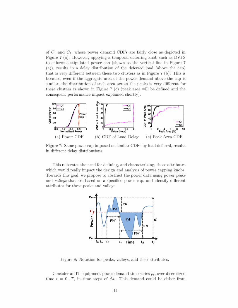
of C1 and C4, whose power demand CDFs are fairly close as depicted inFigure 7 (a). However, applying a temporal deferring knob such as DVFSto enforce a stipulated power cap (shown as the vertical line in Figure 7(a)), results in a delay distribution of the deferred load (above the cap)that is very different between these two clusters as in Figure 7 (b). This isbecause, even if the aggregate area of the power demand above the cap issimilar, the distribution of such area across the peaks is very different forthese clusters as shown in Figure 7 (c) (peak area will be defined and theconsequent performance impact explained shortly).
0.6 0.7 0.8 0.9 10
20
40
60
80
100
Normalized Power
CD
F o
f P
ow
er
C1
C4
PowerCap
0 0.5 1 1.5 20
20
40
60
80
100
Delay (Hour)
CD
F o
f L
oa
d A
bo
ve
Ca
p
C1
C4
0 2 4 6 8 100
20
40
60
80
100
Peak Area (%)
CD
F o
f P
ea
k A
rea
C1
C4
(a) Power CDF (b) CDF of Load Delay (c) Peak Area CDF
Figure 7: Same power cap imposed on similar CDFs by load deferral, resultsin different delay distributions.
This reiterates the need for defining, and characterizing, those attributeswhich would really impact the design and analysis of power capping knobs.Towards this goal, we propose to abstract the power data using power peaksand valleys that are based on a specified power cap, and identify differentattributes for these peaks and valleys.
�����
������ ��
��
��
��
��
����
���
���
��
��
��
��
Figure 8: Notation for peaks, valleys, and their attributes.
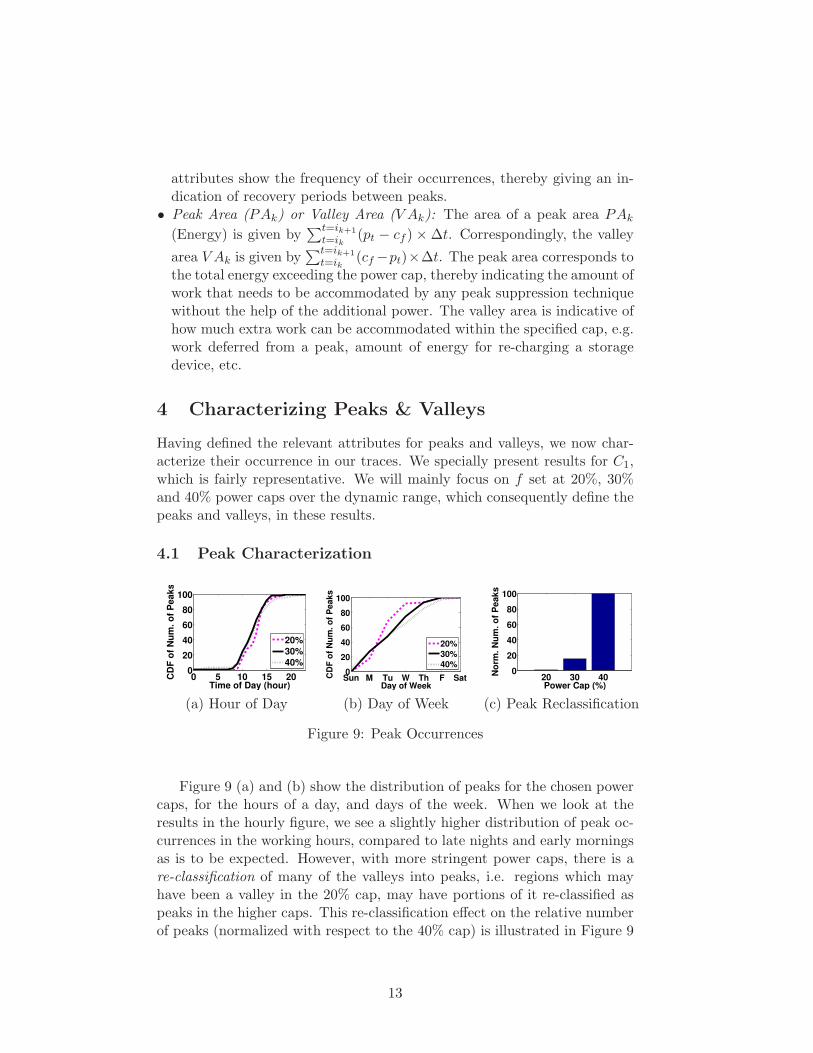
Consider an IT equipment power demand time series pt, over discretizedtime t = 0...T , in time steps of ∆t. This demand could be either from
11

a single server, or a rack, a cluster, or even a datacenter. Let pmin andpmax be the minimum and maximum power demand over all t in this timeseries. The dynamic range of power consumption, denoted d, is given byd = pmax − pmin. For any technique employed to optimize the peak powerconsumption, the scope of options to set the power cap is only within thisdynamic range d. Consequently, we define a power cap cf , in terms of thefraction, f , (percentage) of this dynamic range. The absolute power cap isthen given by cf = (1 − f) × d + pmin. Our experiments in subsequentsections will explore values of f = 20%, 30% and 40%.
Setting a cap of cf to the time series pt gives rise to peaks and valleysin the power draw as illustrated in Figure 8. For instance, the power drawsin the time intervals [t0, ta] and [tb, tc] are example peaks, while the powerdraws in time intervals [ta, tb] and [tc, td] are example valleys in this figure.Formally, we can define a series {i1...ik} of points in time where the powerdemand intersects the horizontal line at a given cf , i.e. ∀t ∈ ik, pt = cf .Note that the power demand in any interval [ik, ik+1] can be categorizedas either a peak or a valley. It is a peak if the power demand within thisinterval exceeds cf , and is a valley otherwise. In addition, we also need toconsider the extreme cases of intervals [t0, i1] and [ik, tT ] where the beginningand end of time series do not intersect with the horizontal line cf . Theseintervals can also be categorized as a peak or a valley depending on whetherthe power demand in those intervals fall above or below cf respectively.
The power demand time series pt, can now be expressed as a sequence ofpeaks and valleys of different intervals defined by their respective [ik, ik+1],with k used to denote the index in the sequence. An interval k, whether apeak or a valley, can be characterized by the following attributes, each ofwhich can have an implication on power capping:
• Peak Height (PHk) or Valley Depth (V Dk): When k is a peak, its height
(Power) can be specified as PHk =maxik≤t≤ik+1
{pt}−cf
d. This is the max-
imum power draw exceeding the defined cap that needs to be providedover the duration of this peak, normalized as a fraction or percentage ofthe dynamic power range d. From a practical viewpoint, the magnitudeof PHk would determine the magnitude of the power capping knob thatis employed to cap this peak, e.g. number of servers that need to beshutdown, the power states in DVFS to be employed, the capacity of anenergy storage device to sustain this peak power need, etc.
Similarly, when k is a valley, its depth can be specified as V Dk =cf−minik≤t≤ik+1
{pt}
d.
This is the lowest power draw during this valley, capturing its ability tore-charge an energy storage device, take on the load deferred from priorpeaks, etc.
• Peak Width (PWk) or Valley Width (V Wk): This is simply the duration(time) of the corresponding peak or valley and is calculated as ik+1 − ik.Valley width corresponds to the inter-peak time and vice-versa. These
12
attributes show the frequency of their occurrences, thereby giving an in-dication of recovery periods between peaks.
• Peak Area (PAk) or Valley Area (V Ak): The area of a peak area PAk
(Energy) is given by∑t=ik+1
t=ik(pt − cf ) × ∆t. Correspondingly, the valley
area V Ak is given by∑t=ik+1
t=ik(cf −pt)×∆t. The peak area corresponds to
the total energy exceeding the power cap, thereby indicating the amount ofwork that needs to be accommodated by any peak suppression techniquewithout the help of the additional power. The valley area is indicative ofhow much extra work can be accommodated within the specified cap, e.g.work deferred from a peak, amount of energy for re-charging a storagedevice, etc.
4 Characterizing Peaks & Valleys
Having defined the relevant attributes for peaks and valleys, we now char-acterize their occurrence in our traces. We specially present results for C1,which is fairly representative. We will mainly focus on f set at 20%, 30%and 40% power caps over the dynamic range, which consequently define thepeaks and valleys, in these results.
4.1 Peak Characterization
0 5 10 15 200
20
40
60
80
100
Time of Day (hour)
CD
F o
f N
um
. o
f P
eaks
20%
30%
40%
Sun M Tu W Th F Sat0
20
40
60
80
100
Day of Week
CD
F o
f N
um
. o
f P
eaks
20%
30%
40%
20 30 400
20
40
60
80
100
No
rm. N
um
. o
f P
eaks
Power Cap (%)
(a) Hour of Day (b) Day of Week (c) Peak Reclassification
Figure 9: Peak Occurrences
Figure 9 (a) and (b) show the distribution of peaks for the chosen powercaps, for the hours of a day, and days of the week. When we look at theresults in the hourly figure, we see a slightly higher distribution of peak oc-currences in the working hours, compared to late nights and early morningsas is to be expected. However, with more stringent power caps, there is are-classification of many of the valleys into peaks, i.e. regions which mayhave been a valley in the 20% cap, may have portions of it re-classified aspeaks in the higher caps. This re-classification effect on the relative numberof peaks (normalized with respect to the 40% cap) is illustrated in Figure 9
13

(c). Such re-classification leads to a more uniform distribution of the num-ber of peaks in the 30% and 40% caps, for the day-of-the-week behavior,with the 20% cap being most influenced by day of the week.
0 10 20 30 400
20
40
60
80
100
Peak Height (%)
CD
F o
f N
um
. o
f P
eaks
20%
30%
40%
Figure 10: Peak Height Distribution
Height Figure 10 shows the CDF of peak heights (PH), across 6 monthduration, for the three power caps. Note that a power cap bounds the max-imum height of a peak, i.e. the right-most point of the CDF. However, asthe figure indicates, a majority of the peaks have small amplitudes. Forexample, with the 20% cap, nearly 90% of the peaks have amplitudes of10% or less, which is less than half the cap magnitude. With more strin-gent caps, while the maximum amplitude can increase, we find that the 30%and 40% caps are still heavily skewed towards the small amplitudes withover 95% of their peaks having amplitudes lower than 10%. This suggeststhat as amplitudes of peaks already selected by the 20% cap get taller inthe 30% and 40% cases, an even larger number of peaks (of smaller ampli-tudes) are being brought in by the re-classification in these stringent caps,thereby slightly shifting their CDF curves to the left. However, the peaksof amplitudes of 20% or higher are non-zero (though visually not apparent),thereby indicating the need for good peak suppression across a wider rangeof amplitudes.
Width Figure 11 shows the CDF of the peak width (PW ) distributionwith the three specified power caps. In the interest of clarity, the x-axis isshown for a zoom-ed in portion of the results. As the caps become morestringent, two factors influence the CDF: (i) more peaks (of smaller widths)get added to the classification, and (ii) existing peaks get wider. Whenmoving from 20% to 30% cap, the former effect is more pronounced, whilewhen moving from 30% to 40%, the rate of addition of new narrow peaksis not sufficient to outweigh the latter widening factor. Regardless of thepower caps, these results show that a vast majority of the peaks are quitenarrow, i.e. nearly 95% of the peaks last only 4 minutes or less. However,there are a few long peaks as well. For instance, the 20%, 30% and 40%
14

0 2 4 6 8 100
20
40
60
80
100
Peak Width (Min)
CD
F o
f N
um
. o
f P
eaks
20%
30%
40%
Figure 11: Peak Width Distribution
caps have a maximum peak width of 50 minutes, 70 minutes, and 4 hours30 minutes respectively, identifying the need to handle a wide span of peakdurations for any peak suppression technique.
Height vs. Width Table 2 shows the distribution of peak heights andwidths under the 40% Cap (results are similar for the other two). In gen-eral, short duration peaks (lasting say 1 minute or shorter, which constitutenearly 80% of the peaks), are also typically shorter in amplitude, comparedto the relatively longer duration peaks. Note that there are peaks lastingover 48 minutes, that do have heights as high as the cap (40%) itself. Eventhough the latter kind occur rarely, their magnitude (both in amplitudeand duration) can be substantial, leading us to investigate the energy needs(corresponding to the work performed) of the different kinds of peaks, as iscaptured by the peak area next.
PHk PWk (Min.)(%) 0-0.5 0.5-1 1-5 5-24 24-48 ≥ 48
0-5 49.29 24.23 8.89 0.13 0 0
5-10 1.62 3.90 7.91 1.02 0 0
10-15 0.13 0.45 0.96 0.51 0.16 0.01
15-20 0 0.07 0.13 0.13 0.06 0.07
20-25 0 0 0.04 0.06 0.01 0.07
25-30 0 0 0.04 0.01 0 0.03
≥ 30 0 0 0 0.03 0 0.03
Table 2: Distribution of Peaks in terms of their Height and Width (as % ofpeaks). f = 40%.
Area The area in a peak (PA) can be a more effective measure of thework that needs to be efficiently handled by any peak suppressing strategy,rather than its height or width alone. Figure 12 (a) shows the distribution
15
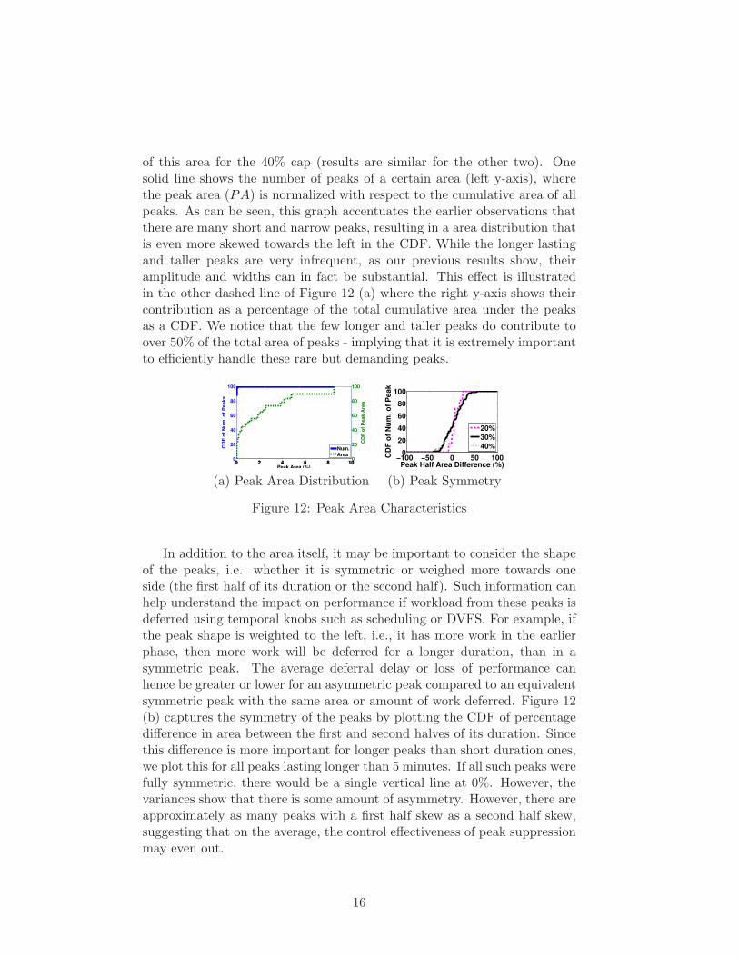
of this area for the 40% cap (results are similar for the other two). Onesolid line shows the number of peaks of a certain area (left y-axis), wherethe peak area (PA) is normalized with respect to the cumulative area of allpeaks. As can be seen, this graph accentuates the earlier observations thatthere are many short and narrow peaks, resulting in a area distribution thatis even more skewed towards the left in the CDF. While the longer lastingand taller peaks are very infrequent, as our previous results show, theiramplitude and widths can in fact be substantial. This effect is illustratedin the other dashed line of Figure 12 (a) where the right y-axis shows theircontribution as a percentage of the total cumulative area under the peaksas a CDF. We notice that the few longer and taller peaks do contribute toover 50% of the total area of peaks - implying that it is extremely importantto efficiently handle these rare but demanding peaks.
0 2 4 6 8 100
20
40
60
80
100
Peak Area (%)
CD
F o
f N
um
. o
f P
ea
ks
0 2 4 6 8 100
20
40
60
80
100
CD
F o
f P
ea
k A
rea
Num.
Area−100 −50 0 50 100
0
20
40
60
80
100
Peak Half Area Difference (%)
CD
F o
f N
um
. o
f P
eak
20%
30%
40%
(a) Peak Area Distribution (b) Peak Symmetry
Figure 12: Peak Area Characteristics
In addition to the area itself, it may be important to consider the shapeof the peaks, i.e. whether it is symmetric or weighed more towards oneside (the first half of its duration or the second half). Such information canhelp understand the impact on performance if workload from these peaks isdeferred using temporal knobs such as scheduling or DVFS. For example, ifthe peak shape is weighted to the left, i.e., it has more work in the earlierphase, then more work will be deferred for a longer duration, than in asymmetric peak. The average deferral delay or loss of performance canhence be greater or lower for an asymmetric peak compared to an equivalentsymmetric peak with the same area or amount of work deferred. Figure 12(b) captures the symmetry of the peaks by plotting the CDF of percentagedifference in area between the first and second halves of its duration. Sincethis difference is more important for longer peaks than short duration ones,we plot this for all peaks lasting longer than 5 minutes. If all such peaks werefully symmetric, there would be a single vertical line at 0%. However, thevariances show that there is some amount of asymmetry. However, there areapproximately as many peaks with a first half skew as a second half skew,suggesting that on the average, the control effectiveness of peak suppressionmay even out.
16
PHk PAk (%)(%) 0-0.01 0.01-0.1 0.1-1 ≥ 1
0-5 80.30 2.24 0 0
5-10 5.98 8.20 0.25 0
10-20 0.19 1.69 0.76 0.07
≥ 20 0 0.08 0.12 0.12
Table 3: Distribution of peaks in terms of their height and area (as % ofpeaks). Area is normalized with respect to the total area under peaks.f = 40%.
Height vs. Area Another important characteristic to understand is theheight vs. area correlations of peaks, since this has a direct bearing onthe choice of technology used in energy storage devices (ESDs) for peaksuppression. Certain ESDs such as ultra-capacitors are more efficient forhandling a large height (power amplitude), while others such as compressedair energy storage are better for large area (energy). Ragone plots in [47]show significant differences in these efficacies using a 2-dimensional (powervs. energy) plot for different ESD technologies, including ultracapacitors,batteries, and compressed air, etc. Table 3 shows the percentage of peakswith different height and area ranges for the 40% power cap. While the bulkof peaks are in the small and narrow bin as already observed, we notice theresults in this table are weighted more along the diagonal. This suggests thatwhile there could be some vagaries, a large number of peaks are probablysuited to a single technology that provides a reasonable trade-off betweenpower vs. energy costs in the Ragone plot (i.e. neither energy biased norpower biased). We will revisit this issue in greater detail in the next section.
4.2 Valley Characterization
0 2 4 6 8 100
20
40
60
80
100
Minute
CD
F o
f p
eaks/v
alleys
Valley
Peak
Figure 13: Valley Width Distribution. f = 30%.
17
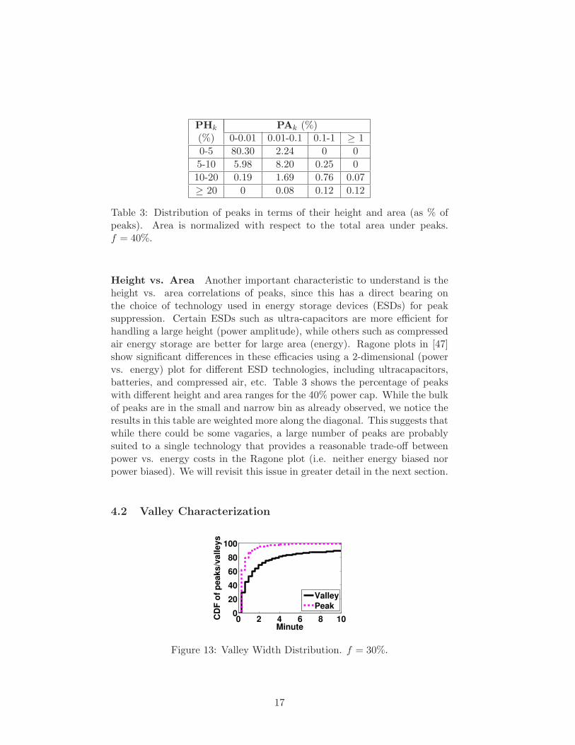
Width Valley width (V W ) measures the inter-peak distance, reflectingthe allowable “quiesce” time from the effects of suppressing the previouspeak (say using scheduling or DVFS), and is also indicative of the durationfor preparing for the next peak (re-charging an ESD, migrating workloads,etc.). Figure 13 shows the CDF of the valley width for the 30% powercap (similar for the other caps), and compares it with the correspondingpeak width distribution. In the interest of clarity, the x-axis is shown for azoom-ed in portion. Valley width is more skewed towards longer durationscompared to the peaks. For instance, 60% of peaks last only up to 30 sec-onds, while 70% of the valleys are of longer duration than 30 seconds. Sincethe valleys are recovery time or preparation periods between peaks, theseresults are suggestive of reasonable slack being available for such recoveryor prepared-ness. However, the magnitude (area) of the valley needs to beclosely examined for more concrete pronouncements as is investigated next.In the interest of space, we merely note that valley depth shows similardistribution as peak height and omit the details for valley depth alone.
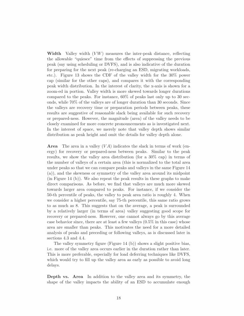
Area The area in a valley (V A) indicates the slack in terms of work (en-ergy) for recovery or prepared-ness between peaks. Similar to the peakresults, we show the valley area distribution (for a 30% cap) in terms ofthe number of valleys of a certain area (this is normalized to the total areaunder peaks so that we can compare peaks and valleys in the same Figure 14(a)), and the skewness or symmetry of the valley area around its midpoint(in Figure 14 (b)). We also repeat the peak results in these graphs to makedirect comparisons. As before, we find that valleys are much more skewedtowards larger area compared to peaks. For instance, if we consider the50-th percentile of peaks, the valley to peak area ratio is roughly 4. Whenwe consider a higher percentile, say 75-th percentile, this same ratio growsto as much as 8. This suggests that on the average, a peak is surroundedby a relatively larger (in terms of area) valley suggesting good scope forrecovery or prepared-ness. However, one cannot always go by this averagecase behavior since, there are at least a few valleys (0.5% in this case) whosearea are smaller than peaks. This motivates the need for a more detailedanalysis of peaks and preceding or following valleys, as is discussed later insections 4.3 and 4.4.
The valley symmetry figure (Figure 14 (b)) shows a slight positive bias,i.e. more of the valley area occurs earlier in the duration rather than later.This is more preferable, especially for load deferring techniques like DVFS,which would try to fill up the valley area as early as possible to avoid longdelays.
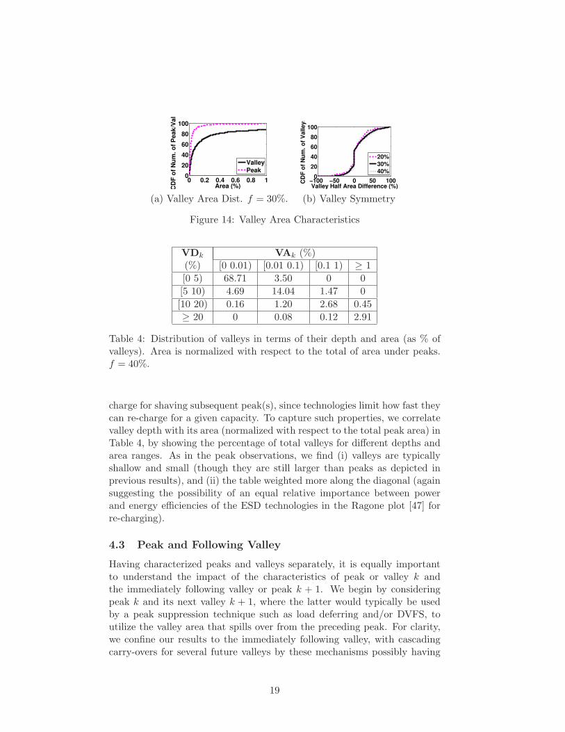
Depth vs. Area In addition to the valley area and its symmetry, theshape of the valley impacts the ability of an ESD to accumulate enough
18
0 0.2 0.4 0.6 0.8 10
20
40
60
80
100
Area (%)CD
F o
f N
um
. o
f P
eak/V
alley
Valley
Peak
−100 −50 0 50 1000
20
40
60
80
100
Valley Half Area Difference (%)
CD
F o
f N
um
. o
f V
alleys
20%
30%
40%
(a) Valley Area Dist. f = 30%. (b) Valley Symmetry
Figure 14: Valley Area Characteristics
VDk VAk (%)(%) [0 0.01) [0.01 0.1) [0.1 1) ≥ 1
[0 5) 68.71 3.50 0 0
[5 10) 4.69 14.04 1.47 0
[10 20) 0.16 1.20 2.68 0.45
≥ 20 0 0.08 0.12 2.91
Table 4: Distribution of valleys in terms of their depth and area (as % ofvalleys). Area is normalized with respect to the total of area under peaks.f = 40%.
charge for shaving subsequent peak(s), since technologies limit how fast theycan re-charge for a given capacity. To capture such properties, we correlatevalley depth with its area (normalized with respect to the total peak area) inTable 4, by showing the percentage of total valleys for different depths andarea ranges. As in the peak observations, we find (i) valleys are typicallyshallow and small (though they are still larger than peaks as depicted inprevious results), and (ii) the table weighted more along the diagonal (againsuggesting the possibility of an equal relative importance between powerand energy efficiencies of the ESD technologies in the Ragone plot [47] forre-charging).
4.3 Peak and Following Valley
Having characterized peaks and valleys separately, it is equally importantto understand the impact of the characteristics of peak or valley k andthe immediately following valley or peak k + 1. We begin by consideringpeak k and its next valley k + 1, where the latter would typically be usedby a peak suppression technique such as load deferring and/or DVFS, toutilize the valley area that spills over from the preceding peak. For clarity,we confine our results to the immediately following valley, with cascadingcarry-overs for several future valleys by these mechanisms possibly having
19

−100 −50 0 50 1000
20
40
60
80
100
(PAk−VA
k+1)/(PA
k+VA
k+1)(%)
CD
F o
f N
um
. o
f P
air
s
20%
30%
40%
Figure 15: Peak and Following Valley
severe performance repercussions. We will, however, discuss such possibleoccurrences and their implications at the end.
There are two main metrics for this consideration - (i) the valley width(V Wk+1) following the peak width (PWk) as depicted in Table 5, and (ii) thevalley area (V Ak+1) following the peak area (PAk) as captured in Figure15. Table 5 shows the percentage of preceding peak and following valleywidths that fall in different duration ranges. It is interesting to view thistable or matrix in upper and lower triangular form. The values in the uppertriangular part indicate the percentage (roughly 46%) of peak-valley pairs,where the subsequent valley is of longer duration than the peak. The valuesin the lower triangular part indicate the possibly “worrisome” percentagewhere the peak is of longer duration than the following valley, i.e. peaks arecoming in closer proximation without ample recovery time for load throttlingor deferring mechanisms. Around 29% of the peak-valley pairs fall in thiscategory.
However, even if the following valley is of shorter duration than thepreceding peak, the deferral or DVFS techniques may still perform well if thevalley has sufficient area (depth) to accommodate the spilled over load. Thisis captured in Figure 15 which shows the CDF of the percentage differencebetween the peak and subsequent valley area. Negative values suggest thatthe valley area dominate over the peaks, while positive values suggest vice-versa. At 20% and 30% caps, over 70% of the valleys have sufficient room totake on any load deferred from the preceding peak. With a more stringentcap of 40%, as many peaks are larger than their corresponding valleys asvice-versa.
The above two sets of results suggest that any load deferral or DVFStechniques should not presume that the immediately following valley willalways have sufficient room to accommodate load spillage from the priorpeak. This is particularly true for the short duration peaks as is evident fromTable 5. Consequently, such peak suppression mechanisms should recognizethe burstiness behavior of these peaks, and employ solutions to addressthem in a grouped or aggregate manner. There are also a few cases where
20

PWk VWk+1 (min)(min) 0-0.5 0.5-1 1-5 5-30 30-60 ≥ 60
0-0.5 13.42 13.23 15.45 5.65 1.00 2.28
0.5-1 11.30 8.83 6.64 1.20 0.20 0.48
1-5 9.63 5.65 1.66 0.13 0.01 0.20
5-30 1.88 0.36 0.12 0.01 0.04 0.21
30-60 0.16 0.03 0 0.03 0.01 0
≥ 60 0.16 0 0.01 0 0 0
Table 5: Peak width vs. following valley width (% of peak-valley pairs).f = 40%.
a longer duration peak is followed by a shorter duration valley, and in suchcases the impact of load deferral techniques will depend not just on thesubsequent valley but also on the subsequent peak(s) (if those are also long,then techniques such as server shutdowns, load migration, etc., may bemandated). This is explored further in section 4.5.
4.4 Peak and the Preceding Valleys
−100 −50 0 50 1000
20
40
60
80
100
(VAk−PA
k+1)/(VA
k+PA
k+1)(%)
CD
F o
f N
um
. o
f P
air
s
20%
30%
40%
−100 −50 0 50 1000
20
40
60
80
100
Σ(VAk−PA
k+1)/Σ(VA
k+PA
k+1)(%)
CD
F
20%
30%
40%
−100 −50 0 50 1000
20
40
60
80
100
Σk
k−10(VA
k−PA
k+1)/Σ
k
k−10(VA
k+PA
k+1(%)
CD
F
20%
30%
40%
(a) Immediate Preced. (b) All valleys till (c) Preceding 10Valley till that peak Valleys
Figure 16: Peak and Preceding Valley(s)
The correlations between a peak and its preceding valleys is important forESD-based peak suppression, which relies on previous valleys to re-chargeits capacity for sourcing power during the current peak. We mainly lookat the area (energy) capacity of the valleys for charging opportunities (inthe interest of space, we merely note that power capacities are typicallyadequate).
Figure 16 (a) captures the area difference of a peak and its precedingvalley. With 20% caps, nearly 80% of the preceding valleys have sufficientenergy charging capacities for the following peak. This percentage decreasesto 60% for the 40% cap. However, note that unlike load deferral and DVFStechniques, ESD based peak suppression does not incur performance penal-
21
PHk PHk+2 (%)(%) 0-5 5-10 10-20 ≥ 20
0-5 72.30 9.02 1.06 0.17
5-10 8.98 4.57 0.87 0.03
10-20 1.12 0.83 0.68 0.07
≥ 20 0.15 0.03 0.09 0.05
Table 6: Distribution of consecutive peak heights (as % of peak-peak pairs).f = 40%
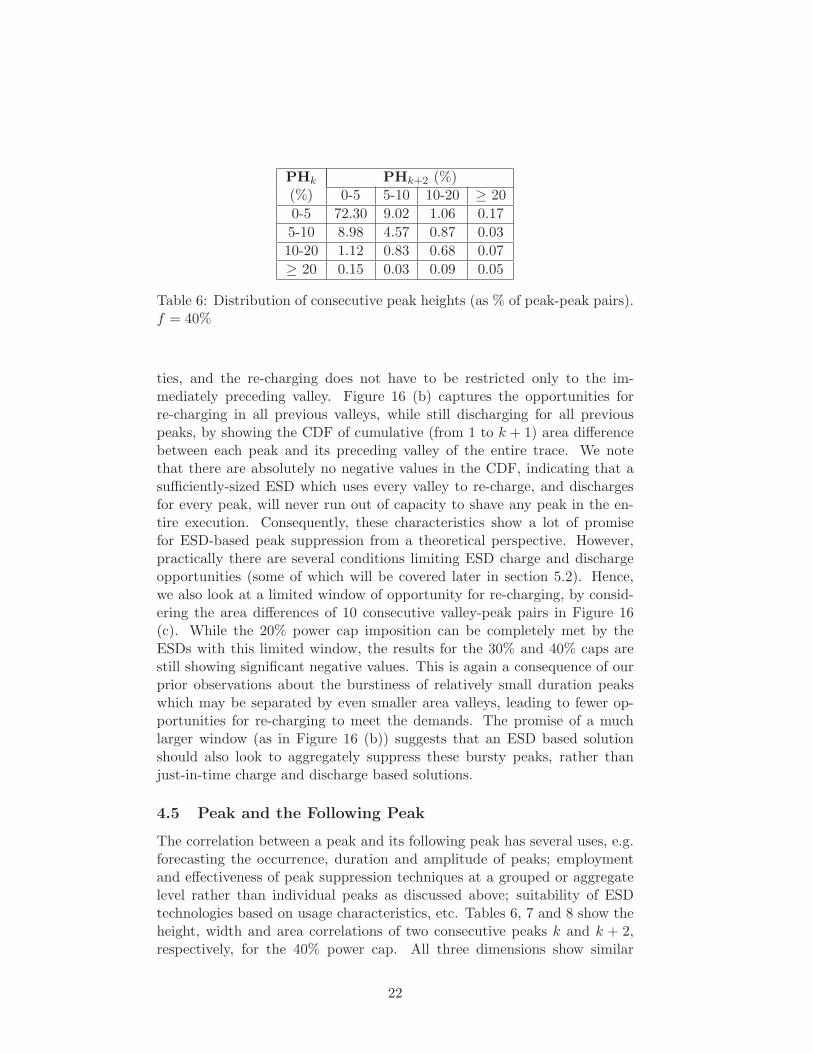
ties, and the re-charging does not have to be restricted only to the im-mediately preceding valley. Figure 16 (b) captures the opportunities forre-charging in all previous valleys, while still discharging for all previouspeaks, by showing the CDF of cumulative (from 1 to k + 1) area differencebetween each peak and its preceding valley of the entire trace. We notethat there are absolutely no negative values in the CDF, indicating that asufficiently-sized ESD which uses every valley to re-charge, and dischargesfor every peak, will never run out of capacity to shave any peak in the en-tire execution. Consequently, these characteristics show a lot of promisefor ESD-based peak suppression from a theoretical perspective. However,practically there are several conditions limiting ESD charge and dischargeopportunities (some of which will be covered later in section 5.2). Hence,we also look at a limited window of opportunity for re-charging, by consid-ering the area differences of 10 consecutive valley-peak pairs in Figure 16(c). While the 20% power cap imposition can be completely met by theESDs with this limited window, the results for the 30% and 40% caps arestill showing significant negative values. This is again a consequence of ourprior observations about the burstiness of relatively small duration peakswhich may be separated by even smaller area valleys, leading to fewer op-portunities for re-charging to meet the demands. The promise of a muchlarger window (as in Figure 16 (b)) suggests that an ESD based solutionshould also look to aggregately suppress these bursty peaks, rather thanjust-in-time charge and discharge based solutions.
4.5 Peak and the Following Peak
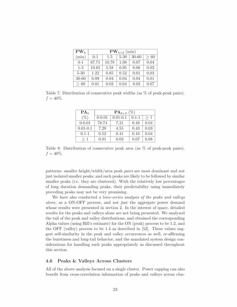
The correlation between a peak and its following peak has several uses, e.g.forecasting the occurrence, duration and amplitude of peaks; employmentand effectiveness of peak suppression techniques at a grouped or aggregatelevel rather than individual peaks as discussed above; suitability of ESDtechnologies based on usage characteristics, etc. Tables 6, 7 and 8 show theheight, width and area correlations of two consecutive peaks k and k + 2,respectively, for the 40% power cap. All three dimensions show similar
22
PWk PWk+2 (min)(min) 0-1 1-5 5-30 30-60 ≥ 60
0-1 67.71 10.78 1.08 0.07 0.04
1-5 10.65 5.58 0.95 0.08 0.03
5-30 1.22 0.85 0.52 0.01 0.03
30-60 0.09 0.04 0.04 0.04 0.01
≥ 60 0.01 0.03 0.04 0.03 0.07
Table 7: Distribution of consecutive peak widths (as % of peak-peak pairs).f = 40%.
PAk PAk+2 (%)(%) 0-0.01 0.01-0.1 0.1-1 ≥ 1
0-0.01 78.74 7.21 0.48 0.04
0.01-0.1 7.20 4.55 0.43 0.03
0.1-1 0.52 0.41 0.16 0.04
≥ 1 0.01 0.03 0.07 0.08
Table 8: Distribution of consecutive peak area (as % of peak-peak pairs).f = 40%.
patterns: smaller height/width/area peak pairs are most dominant and notjust isolated smaller peaks; and such peaks are likely to be followed by similarsmaller peaks (i.e. they are clustered). With the relatively low percentagesof long duration demanding peaks, their predictability using immediatelypreceding peaks may not be very promising.
We have also conducted a time-series analysis of the peaks and valleysalone, as a ON-OFF process, and not just the aggregate power demandwhose results were presented in section 2. In the interest of space, detailedresults for the peaks and valleys alone are not being presented. We analyzedthe tail of the peak and valley distributions, and obtained the correspondingAlpha values (using Hill’s estimate) for the ON (peak) process to be 1.2, andthe OFF (valley) process to be 1.4 as described in [52]. These values sug-gest self-similarity in the peak and valley occurrences as well, re-affirmingthe burstiness and long-tail behavior, and the mandated system design con-siderations for handling such peaks appropriately as discussed throughoutthis section.
4.6 Peaks & Valleys Across Clusters
All of the above analysis focused on a single cluster. Power capping can alsobenefit from cross-correlation information of peaks and valleys across clus-
23

ters, to better multiplex the aggregate demand and even migrate the loadaccordingly. As noted in previous studies [12, 47], power under-provisioningis important at multiple layers of the datacenter power hierarchy, and clus-ter level capping may become necessary in such cases as opposed to justexploiting multiplexing characteristics at the higher (datacenter) level. Wehave conducted cross-cluster correlation analysis, and simply summarize theresults using two metrics, in the interest of space, for clusters C1 and C2,with f = 40% in both and the numbers are similar across other clusters aswell. The first is the probability of a simultaneous peak occurrence in bothclusters which we find to be extremely low, i.e. only 0.1% of the time isthere a simultaneous peak on both clusters. The second measures whethershifting the peak from one cluster to the other leads to a consequent peak onthe latter. We find that this probability is also quite low, with less than 2%of the time that a peak movement to the other cluster results in an exceedingof the cap in the latter. These results suggest the potential of multiplexingwhich was alluded to some extent in the aggregate characteristics of section2. More importantly, re-distribution of load has tremendous potential inpeak suppression, as long as we do not perform such re-distribution too fre-quently for this to become an overhead by itself. We will illustrate how suchspatial differences across clusters, and the temporal analysis of this section,can be used to fine-tune the peak capping knobs in the following section.
5 Exploiting Characteristics
There are several use-cases for exploiting the characteristics quantified inthe previous section. Some of these include (i) the ability to predict theimpact of power capping knobs (which was motivated earlier in Figure 7),(ii) predicting and preparing for the occurrences of future peaks and val-leys, (iii) synthesizing workloads to facilitate research on power optimiza-tions, (iv) developing and fine-tuning power capping knobs based on thepower characteristics, (v) capacity provisioning for the datacenter for bet-ter power-performance trade-offs, among others. We illustrate the utility ofsuch characterization with two case studies. The first exploits the charac-teristics to fine-tune temporal load deferring and spatial migration knobs,leveraging information about peak-valley behaviors. The second uses thecharacteristics to come up with a simple capacity provisioning technique forenergy storage in the datacenter, to suppress peaks.
5.1 Tuning Knobs based on Characteristics
As observed in the previous section, both small peaks (which are numerous)and large peaks (though infrequent but extremely demanding) are equallyimportant for peak shaving. One could use a one-size-fits-all policy to shaveall the peaks, say using temporal load deferring (LD) to the immediate next
24
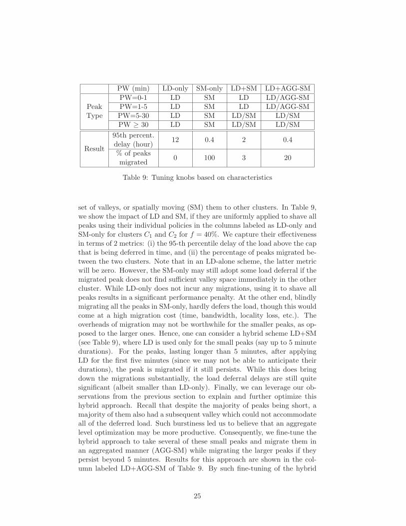
PW (min) LD-only SM-only LD+SM LD+AGG-SM
PW=0-1 LD SM LD LD/AGG-SMPeak PW=1-5 LD SM LD LD/AGG-SMType PW=5-30 LD SM LD/SM LD/SM
PW ≥ 30 LD SM LD/SM LD/SM
Result
95th percent.12 0.4 2 0.4
delay (hour)% of peaks
0 100 3 20migrated
Table 9: Tuning knobs based on characteristics
set of valleys, or spatially moving (SM) them to other clusters. In Table 9,we show the impact of LD and SM, if they are uniformly applied to shave allpeaks using their individual policies in the columns labeled as LD-only andSM-only for clusters C1 and C2 for f = 40%. We capture their effectivenessin terms of 2 metrics: (i) the 95-th percentile delay of the load above the capthat is being deferred in time, and (ii) the percentage of peaks migrated be-tween the two clusters. Note that in an LD-alone scheme, the latter metricwill be zero. However, the SM-only may still adopt some load deferral if themigrated peak does not find sufficient valley space immediately in the othercluster. While LD-only does not incur any migrations, using it to shave allpeaks results in a significant performance penalty. At the other end, blindlymigrating all the peaks in SM-only, hardly defers the load, though this wouldcome at a high migration cost (time, bandwidth, locality loss, etc.). Theoverheads of migration may not be worthwhile for the smaller peaks, as op-posed to the larger ones. Hence, one can consider a hybrid scheme LD+SM(see Table 9), where LD is used only for the small peaks (say up to 5 minutedurations). For the peaks, lasting longer than 5 minutes, after applyingLD for the first five minutes (since we may not be able to anticipate theirdurations), the peak is migrated if it still persists. While this does bringdown the migrations substantially, the load deferral delays are still quitesignificant (albeit smaller than LD-only). Finally, we can leverage our ob-servations from the previous section to explain and further optimize thishybrid approach. Recall that despite the majority of peaks being short, amajority of them also had a subsequent valley which could not accommodateall of the deferred load. Such burstiness led us to believe that an aggregatelevel optimization may be more productive. Consequently, we fine-tune thehybrid approach to take several of these small peaks and migrate them inan aggregated manner (AGG-SM) while migrating the larger peaks if theypersist beyond 5 minutes. Results for this approach are shown in the col-umn labeled LD+AGG-SM of Table 9. By such fine-tuning of the hybrid
25
approach, the migrations have dropped substantially, and the load defer-ral delays are quite comparable to the SM-only approach, thus performingbetter than the LD-only and SM-only approaches individually.
Note that our goal is not to come up with the best peak shaving optionin this study. Rather, our point is to illustrate that our characterization canbe used to fine-tune such decisions.
5.2 ESD Provisioning
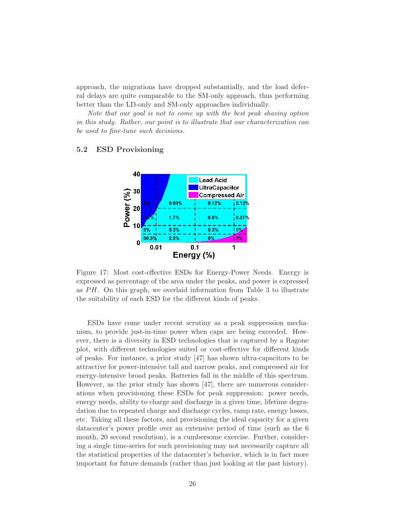
Figure 17: Most cost-effective ESDs for Energy-Power Needs. Energy isexpressed as percentage of the area under the peaks, and power is expressedas PH. On this graph, we overlaid information from Table 3 to illustratethe suitability of each ESD for the different kinds of peaks.
ESDs have come under recent scrutiny as a peak suppression mecha-nism, to provide just-in-time power when caps are being exceeded. How-ever, there is a diversity in ESD technologies that is captured by a Ragoneplot, with different technologies suited or cost-effective for different kindsof peaks. For instance, a prior study [47] has shown ultra-capacitors to beattractive for power-intensive tall and narrow peaks, and compressed air forenergy-intensive broad peaks. Batteries fall in the middle of this spectrum.However, as the prior study has shown [47], there are numerous consider-ations when provisioning these ESDs for peak suppression: power needs,energy needs, ability to charge and discharge in a given time, lifetime degra-dation due to repeated charge and discharge cycles, ramp rate, energy losses,etc. Taking all these factors, and provisioning the ideal capacity for a givendatacenter’s power profile over an extensive period of time (such as the 6month, 20 second resolution), is a cumbersome exercise. Further, consider-ing a single time-series for such provisioning may not necessarily capture allthe statistical properties of the datacenter’s behavior, which is in fact moreimportant for future demands (rather than just looking at the past history).
26

Our characterization results, presented in the previous section, can provideone possibly simple methodology for ESD provisioning, even if it is not theoptimal, as discussed below.
Choosing Technology: Given a peak of height PH and area PA, thecapacity of an ESD and hence its cost (C) to shave this peak can be de-termined by its technology’s power (CP ) and energy (CE) density cost asC = max
(
PH × CP , PA × CE)
. Using this simple model, we compute the(PH, PA) regions over which 3 ESD technologies (Ultra-capacitor, Leadacid battery, and Compressed air energy storage) under consideration arethe most cost-effective as in Figure 17. We can overlay the PH and PA
distributions from Table 3 on this figure, to examine the suitability of eachtechnology to shave a certain number of peaks. We see that a majority(99.8%) of peaks from Table 3 falls in the region where lead-acid battery isthe most cost effective technology. Very few (0.2%) of the peaks fall in theultra-capacitor region, and this constitutes only about 0.1% of the area ofthe peaks. Consequently, we can simply go with the lead-acid battery op-tion, amongst the 3 technology choices based on our characteristics results.
Quantifying Capacity: The shape - height which indicates peak power,and area which indicates energy needs - of the peaks determines the requiredESD capacity for any given technology. We, thus, examine the characteris-tics in Figure 10 and Figure 12 (a). Rather than go for the 100-th percentile,we pick the knees of these curves - 90th percentile of the peaks in terms ofheight, peaks contributing to the 90% of total area under peaks - with theformer indicating the power capacity and the latter representing the requiredenergy capacity. The maximum between these two is what needs to be pro-visioned. However, we also need to ensure that there is sufficient slack in thevalleys to re-charge for this capacity. For this purpose, we examine Figure 16to examine the re-charging opportunities. While the immediately precedingvalley(s) may not have enough slack for such re-charge (Figures 16 (a) and(c)), the results in Figure 16 (b) suggests that greedily re-charging at everyopportunity may provide the slack to re-charge for this capacity to suppressall peaks.
Using these rules-of-thumb as a heuristic for ESD provisioning, in Table10 we show the capacity selected by this heuristic for 2 specific ESD tech-nologies - lead-acid batteries, and ultra-capacitors, showing its effectivenessin shaving the peaks (both number and area). We compare these resultswith an Optimal capacity provisioning algorithm, that is guaranteed to pro-vide the minimal capacity to shave all peaks in the given data. While thelatter does need to extensively run through the time series of power de-mands, to ensure these guarantees (minimal capacity, charge/discharge rateguarantees, account for energy losses, etc.), we find that our simple heuristicapproach shaves over 99% of the peaks, and nearly 90% of the peak area,with a capacity (and corresponding cost), that is less than half of the ca-pacity (for lead-acid batteries) than what the Optimal algorithm specifies.
27

As is evident in Figure 17, lead-acid is an over-whelming favorite as far astechnology is concerned.
Tech. Approach Capacity Cost Peaks shaved Area shaved(% peak (% of (% of total (% of total
area) Opt LA) peaks) peak area)
LA Heuristic 6.0 47 99.97 89.42
LA Opt. 12.1 100 100 100
UC Heuristic 6.0 789 99.97 89.43
UC Opt. 10.8 1494 100 100
Table 10: ESD capacity provisioning for Lead Acid (LA) battery and Ultra-capacitor (UC).
6 Concluding Remarks & Future Work
We have undertaken a detailed characterization of power measurements ofgeo-distributed datacenters of Microsoft corporation at fine temporal andspatial resolutions over a 6 month duration. Aggregate analysis of such rawdata shows (i) statistical multiplexing of power demands that can enablemore aggressive under-provisioning at higher layers of the power hierarchy;(ii) significant evidence of self-similarity in the power demands, togetherwith time-of-day behavior; and (iii) correlations between the IT and cool-ing power, with the latter showing higher variance, and a 2-minute lag be-hind the former. While these aggregate characteristics can be useful bythemselves, there is a need for better abstractions to design, evaluate, andfine-tune peak suppression mechanisms to achieve a desired level of powercapping. Towards this goal, this paper has made the following contributions:Abstractions: We have formally defined peaks and valleys, their importantattributes (height, width, area), and the correlations between peaks andvalleys that need to be studied towards designing and understanding thepotential of any peak suppression mechanism.Characterizing Peaks and Valleys: We have extensively characterized peakand valley attributes individually, and their cross-correlations. Results showthat while there are an overwhelming number of small duration and smallamplitude peaks, we cannot afford to ignore the few large ones that havevery stringent demands. Further, while on the average, valleys do offerenough slack for load deferment or peak preparation, there are bursts ofpeaks which do not have sufficient valleys immediately following or precedingthem. Further, there is significant potential of migrating load to exploitpeaks and valleys across clusters, as long as we can restrict the numberof such migrations to avoid the consequent performance penalties. These
28
suggest aggregated optimizations of peaks and valleys.Exploiting Characteristics: There are numerous use-cases for our character-istics, and we illustrated two specific case-studies in the limited space of thispaper. The first used the characteristics to fine-tune load deferring and mi-gration based on the kinds of peaks, in an aggregated manner. The secondshowed a simple approach to energy storage provisioning that only uses ag-gregate characteristics, rather than an extensive approach considering everypossible eventuality in the entire power demand time series.
There are several more opportunities for future work to leverage the pro-posed characterizations, including further use of predictability of peak andvalley characteristics for fine-tuning peak suppression knobs, synthesizingworkloads with the broad statistical properties that we have identified, an-alytical models to work with the characteristics for quick performance andcapacity provisioning estimates, energy supply side sourcing and manage-ment issues (including renewables and cost) as opposed to just demand-sidecapping.
References
[1] M. F. Arlitt and C. L. Williamson. Web server workload character-ization: the search for invariants. In Proceedings of SIGMETRICS,1996.
[2] A. A. Bhattacharya, D. Culler, A. Kansal, S. Govindan, and S. Sankar.The need for speed and stability in data center power capping. InProceedings of IGCC, 2012.
[3] R. Bianchini and R. Rajamony. Power and Energy Management forServer Systems. Computer, 37(11), 2004.
[4] D. Brooks, V. Tiwari, and M. Martonosi. Wattch: a framework forarchitectural-level power analysis and optimizations. In Proceedings ofISCA, 2000.
[5] G. Chen, W. He, J. Liu, S. Nath, L. Rigas, L. Xiao, and F. Zhao.Energy-aware server provisioning and load dispatching for connection-intensive internet services. In Proceedings of NSDI, 2008.
[6] M. Crovella and A. Bestavros. Self-similarity in world wide web traffic:evidence and possible causes. IEEE/ACM Transanctions on Network-ing, 5(6):835–846, 1997.
[7] J. Davis, S. Rivoire, M. Goldszmidt, and E. K. Ardestani. IncludingVariability in Large-Scale Cluster Power Models. Computer Architec-ture Letters, 2011.
29
[8] N. Deng, C. Stewart, D. Gmach, M. Arlitt, and J. Kelley. Adaptivegreen hosting. In Proceedings of ICAC, 2012.
[9] Duke utility bill tariff. http://www.duke-energy.com/pdfs/
scscheduleopt.pdf.
[10] D. Economou, S. Rivoire, and C. Kozyrakis. Full-system power analysisand modeling for server environments. In Workshop on MOBS, 2006.
[11] N. El-Sayed, I. A. Stefanovici, G. Amvrosiadis, A. A. Hwang, andB. Schroeder. Temperature management in data centers: why some(might) like it hot. In Proceedings of SIGMETRICS, 2012.
[12] X. Fan, W.-D. Weber, and L. A. Barroso. Power Provisioning for aWarehouse-sized Computer. In Proceedings of ISCA, 2007.
[13] W. Felter, K. Rajamani, C. Rusu, and T. Keller. A Performance-Conserving Approach for Reducing Peak Power Consumption in ServerSystems. In Proceedings of ICS, 2005.
[14] M. E. Femal and V. W. Freeh. Safe overprovisioning: Using powerlimits to increase aggregate throughput. In Workshop on PACS, 2004.
[15] A. Gandhi, M. Harchol-Balter, R. Das, and C. Lefurgy. Optimal powerallocation in server farms. In Proceedings of SIGMETRICS, 2009.
[16] A. Gandhi, M. Harchol-Balter, and M. A. Kozuch. The case for sleepstates in servers. In Workshop on HotPower, 2011.
[17] L. Ganesh, J. Liu, S. Nath, G. Reeves, and F. Zhao. Unleash StrandedPower in Data Centers with RackPacker. In Workshop on WEED, 2009.
[18] M. W. Garrett and W. Willinger. Analysis, modeling and generationof self-similar VBR video traffic. In Proceedings of SIGCOMM, 1994.
[19] D. Gmach, J. Rolia, L. Cherkasova, and A. Kemper. Workload anal-ysis and demand prediction of enterprise data center applications. InProceedings of IISWC, 2007.
[20] S. Govindan, J. Choi, B. Urgaonkar, A. Sivasubramaniam, andA.Baldini. Statistical profiling-based techniques for effective power pro-visioning in data centers. In Proceedings of EUROSYS, 2009.
[21] S. Govindan, A. Sivasubramaniam, and B. Urgaonkar. Benefits andLimitations of Tapping into Stored Energy For Datacenters. In Pro-ceedings of ISCA, 2011.
[22] S. Govindan, D. Wang, A. Sivasubramaniam, and B. Urgaonkar. Lever-aging Stored Energy for Handling Power Emergencies in AggressivelyProvisioned Datacenters. In Proceedings of ASPLOS, 2012.
30

[23] A. Gulati, C. Kumar, and I. Ahmad. Modeling workloads and devicesfor IO load balancing in virtualized environments. SIGMETRICS Per-form. Eval. Rev., 37(3), 2010.
[24] J. Hamilton. Internet-scale Service Infrastructure Efficiency, ISCAKeynote 2009.
[25] A. K. Iyengar, M. S. Squillante, and L. Zhang. Analysis and charac-terization of large-scale web server access patterns and performance.World Wide Web, 2(1-2), 1999.
[26] A. Kansal, F. Zhao, J. Liu, N. Kothari, and A. A. Bhattacharya. Virtualmachine power metering and provisioning. In Proceedings of SOCC,2010.
[27] A. Khan, X. Yan, S. Tao, and N. Anerousis. Workload characteriza-tion and prediction in the cloud: A multiple time series approach. InProceedings of NOMS, 2012.
[28] V. Kontorinis, L. E. Zhang, B. Aksanli, J. Sampson, H. Homayoun,E. Pettis, D. M. Tullsen, and T. S. Rosing. Managing Distributed UPSEnergy for Effective Power Capping in Data Centers. In Proceedings ofISCA, 2012.
[29] B. Krishnan, H. Amur, A. Gavrilovska, and K. Schwan. VM powermetering: feasibility and challenges. SIGMETRICS Performance Eval-uation Review, 38(3):56–60, 2010.
[30] K. Le, R. Bianchini, M. Martonosi, and T. Nguyen. Cost- and energy-aware load distribution across data centers. In Workshop on HotPower,2009.
[31] C. Lefurgy, X. Wang, and M. Ware. Server-Level Power Control. InProceedings of ICAC, 2007.
[32] W. E. Leland, M. S. Taqqu, W. Willinger, and D. V. Wilson. On theself-similar nature of ethernet traffic (extended version). IEEE/ACMTrans. Netw., 2(1), 1994.
[33] Z. Liu, M. Lin, A. Wierman, S. H. Low, and L. L. H. Andrew. Greeninggeographical load balancing. In Proceedings of SIGMETRICS, 2011.
[34] K. Ma, X. Li, M. Chen, and X. Wang. Scalable power control for many-core architectures running multi-threaded applications. In Proceedingsof ISCA, 2011.
[35] J. C. McCullough, Y. Agarwal, J. Chandrashekar, S. Kuppuswamy,A. C. Snoeren, and R. K. Gupta. Evaluating the effectiveness of model-based power characterization. In Proceedings of USENIX, 2011.
31

[36] D. Meisner, C. M. Sadler, L. A. Barroso, W. Weber, and T. F. Wenisch.Power management of online data-intensive services. In Proceedings ofISCA, 2011.
[37] S. Pelley, D. Meisner, P. Zandevakili, T. F. Wenisch, and J. Underwood.Power Routing: Dynamic Power Provisioning in the Data Center. InProceedings of ASPLOS, 2010.
[38] R. Raghavendra, P. Ranganathan, V. Talwar, Z. Wang, and X. Zhu.No Power Struggles: Coordinated multi-level power management forthe data center. In Proceedings of ASPLOS, 2008.
[39] P. Ranganathan, P. Leech, D. Irwin, and J. Chase. Ensemble-levelPower Management for Dense Blade Servers. In Proceedings of ISCA,2006.
[40] A. Riska and E. Riedel. Disk drive level workload characterization. InProceedings of USENIX, 2006.
[41] M. Satyanarayanan. A study of file sizes and functional lifetimes. InProceedings of SOSP, 1981.
[42] B. Schroeder, E. Pinheiro, and W.-D. Weber. DRAM errors in the wild:a large-scale field study. In Proceedings of SIGMETRICS, 2009.
[43] K. Shen, A. Shriraman, S. Dwarkadas, and X. Zhang. Power and energycontainers for multicore servers. In Proceedings of SIGMETRICS, 2012.
[44] A. Vasan, A. Sivasubramaniam, V. Shimpi, T. Sivabalan, and R. Sub-biah. Worth their watts? - an empirical study of datacenter servers. InProceedings of HPCA, 2010.
[45] A. Verma, G. Dasgupta, T. K. Nayak, P. De, and R. Kothari. Serverworkload analysis for power minimization using consolidation. In Pro-ceedings of USENIX, 2009.
[46] A. Verma, P. De, V. Mann, T. Nayak, A. Purohit, G. Dasgupta, andR. Kothari. Brownmap: Enforcing power budget in shared data centers.In Proceedings of MIDDLEWARE, 2010.
[47] D. Wang, C. Ren, A. Sivasubramaniam, B. Urgaonkar, and H. Fathy.Energy storage in datacenters: what, where, and how much? In Pro-ceedings of SIGMETRICS, 2012.
[48] X. Wang and M. Chen. Cluster-level feedback power control for per-formance optimization. In Proceedings of HPCA, 2008.
[49] X. Wang, M. Chen, and C. Lefurgy. How much power oversubscriptionis safe and allowed in data centers? In Proceedings of ICAC, 2011.
32
[50] A. Weisel and F. Bellosa. Process cruise control-event-driven clockscaling for dynamic power management. In Proceedings of CASES,2002.
[51] A. Wierman, L. L. H. Andrew, and A. Tang. Power-aware speed scalingin processor sharing systems: Optimality and robustness. Perform.Eval., 69(12):601–622, 2012.
[52] W. Willinger, M. S. Taqqu, R. Sherman, and D. V. Wilson. Self-similarity through high-variability: statistical analysis of ethernet lantraffic at the source level. In Proceedings of SIGCOMM, 1995.
33