ACI MATERIALSJOURNAL TECHNICAL PAPER Title no. 84-M4

Statistical Extrapolation of Shrinkage Data-Part I: Regression

by Z. P. Ba2ant, F. H. Wittmann, J. K. Kim, and F. Alou

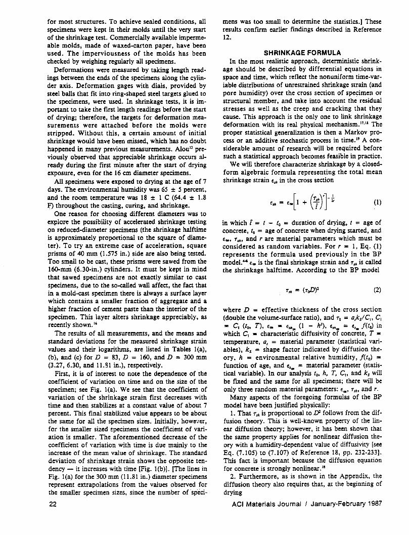
A large series of dala on carefu/ly COnlrolled shrinkage tests of con­crete involving groups of large numbers of identical specimens is re­porttd. The data are used to compare existing shrinkage formulas in ACI, CEB-FIP, and BP models. By far the besl agreement is ob­tained for the BP model. Assuming that only the measured data for a certain initial period are known, predictions are made for long times and are compared with the subsequently observed shrinkage strains. In this manner, various possible statisllca/ regression modeis are ex­amined and compared. Best predictions are obtained when the shrinkage formula is fitted to lest data using nonlinear optimi;,ation, then linear regression in transformed variables is used to obtain the confidence limits for long-time predictions.

It is concluded that good long-time predictions of shrinkage can be obtained on the basis of shrinkage lest results on 80 mm diameter cylinders for a 3-week duration. These predictions involve only the intrinsic uncertainty of the material, on which the uncertainly due to random enVironment, curing history, and differences in concrete composition must be superimposed for practical application.

Keywords: concretes; deformation; diffusion: drying: errors; extrapolation; recreNlOD ••• Iysis: shrinkage: statistical analysis; volume change.

Shrinkage, as well as creep, represents the most un­certain mechanical property of concrete, the statistical scatter of which considerably exceeds that of strength. Yet, in contrast to the design of structures for ultimate loads, the design for shrinkage is not currently based on statistical concepts. The aim of this paper is to estab­lish the statistical properties of shrinkage that could be used in design. This is of interest especially for special structures sensitive to long-time deformations and cracking.

Prediction of shrinkage effects in structures can be made in two phases. The first phase, which is examined here, consists of determining the shrinkage properties of the material, and the second phase consists of the structural analysis based on these properties. The sec­ond phase, which inevitably involves the uncertainty of the method of structural analysis, is not covered here. The uncertainty involved in the first phase has five dis­tinct sources:

1. The uncertainty due to the measurement error. 2. The uncertainty due to random variations of the

environmental relative humidity and temperature.

20

3. The uncertainty due to the random variability of the material properties which results from the process of mixing, casting, and curing of concrete.

4. The uncertainty due to the random nature of shrinkage increments, which is a consequence of the stochastic nature of the microscopic physical mecha­nism of shrinkage.

S. The uncertainty of the shrinkage prediction model per se (i.e., the shrinkage formula), both its form and the values of its parameters.

The first source of uncertainty is not felt by the structure and should, therefore, be minimized by care­ful control of measurements. Proper smoothing of the results can also eliminate much of the random mea~ surement error, although not its systematic part. The second source of uncertainty, which can be most effec­tively treated by spectral analysis of stochastic pro­cesses, has been the subject of other works I·) and will not be studied here. This type of uncertainty is impor­tant for real structures. but it is negligible for tests in a laboratory with good environmental control. There­fore, we strive to model only the third through fifth sources of. uncertainty. These three sources together represent the material, or intrinsic. uncertainties, as opposed to the environmental influences which repre­sent an external, or extrinsic, uncertainty.

The model uncertainty, due to the error of the shrinkage formula, is inevitable since without a mathe­matical model no statistical evaluation is possible. For the formulas used in the current codes. this uncertainty is huge. Statistics involving many thousands of data points from the literature have recently been re­ported,6-6 and it has been found that the confidence limits that are exceeded by the errors with a 10 percent probability are about :t 86 percent of the predicted value for the current ACI 209 model,1,1 and :t 118 per­cent for the current CEB-FIP Model Code. 9 For the re-

Received Sept. 3. 1985, and reviewed under Institute publication polk •••. COPYright @ 1987, Amcncan Concrete Institute. All rights reserved, mcludlftJ the makins of copies unless permiSSion is obtamed from the copyngllt proPV etOfS. Pertinent dlSClluion wiU be published lD thc November-December 19 A CI Mal~rials Journai if received by Aug. I, 1987.

ACI Materials Journal I January-February 1987

z. P. BIII.JuU, FACI, is a profGSOr and dineror, Qnter for Concrete and Geo­materials, Northwestern University. Dr. Bdant is a r~gistered structural engineer, grvu II.S consultant to Argonn~ National lAboratory and several other firms, and is on editorilll boards of five jountllis. He is Chairman of ACI CommillH #6, Fracture Meclulnics, Ilnd 11 memw oj ACI Committee 209, Creep Ilnd Shrinkage in Concrete: 348, Structural Safety: and joint ACI·ASCE Committee 334, Concret~ Shell Design and Construction. He also s~rvu II.S

Clulirman of RILEM CommittH TC69 on creep, of ASCE·EMD CommittH on PropertiG of Materials, and of IA-5MiRT Division H. His works on concrete Ilnd g~omat~ria/s, in~/lI.Stic ~hllvior, fracture and stability hllv~ bun recog· nized by a RILEM medal, ASCE Hu~r Prize and T. Y. Lin Award, IR·lOO A _rd, Guggenheim Fellowship, Ford Foundation Fellowship, and election II.S

Fellow of American Academy of Mechanics.

ACI mem~r F. H. Wlmnllfln is a professor and di~tor of th~ lAboratory for Buildin, Materials, Swiss Federal Institute of TeChnology, Lllusllnne. H~ ~ived th~ RILEM medal for his r_rch on properties of hardened ~ mrnt f1II.St~. H~ :serves II.S chairman of RILEM TC SfJ.FMC, Fracture Mechan· ics of Concr~te, and of RlLEM TC 78·MCA, Mod~1 Cod~ for Autoclaved Aerated Concrete. H~ is on the editorial board of ~ral scientific journals. At present he is presid~nt of the Internlltional Association for Structural Mechan. ics in Reactor Technology and he holds the position of Honorary AdvisOry Professor at Tongji University, Shanghai, China.

ACI mem~r J. K. Kim is Iln lUSistant professor in Civil Engineering at Korea Advanced Institute of Sci~nce and Technology. He obtained his BS Ilnd MS de­gret!S from Seoul National University, and the PhD degree from Northwest~rn University. He is on the edilorilll board of the Journal of the Architectural In· stitute of Korea. His research interests includ~ inelastic ~havior and fracture of concrete and reinforced concrete.

F. Alou receiv~d his diploma in civil engineering at th~ Swiss F~deral Insti· tut~ of T~chnology, lAUSllnn~. At pres~nt he is head of th~ concret~ technol· ogy and materials testing section of the Laboratory for Building Materials, Swiss Fed~ral Institut~ of Technology, LItUSllnn~. For gveral years he direct~d specilll projects in civil engineering in Swit:r.ulllnd Ilnd in Brazil. His research aClivitiG an orirnted toWQrds the relation ~tween the structure of concret~ Ilnd creep and shrinka,~.

cently established shrinkage formulas of the BP model,4-6·lo which is better justified physically but is also more complicated, these confidence limits are found to be ± 27 percent, which is still quite large.

From some limited examples it appears6 that the un­certainty of shrinkage prediction can be drastically re­duced if some short-time measurements of shrinkage of the particular concrete under consideration are made. The question of how to extrapolate such short-time data to obtain long-time shrinkage predictions and their standard deviations will be the principal goal of the analysis that follows.

Part II of this study will deal with the problem of how the long-time predictions can be improved by means of Bayesian reasoning. Another paperll exam­ines the type of probability distributions of strains as well as strain increments, the correlation of short-time and long-time data, and the evolution of statistics with time.

STATISTICAL TeST DATA Abundant as the test data on shrinkage in the litera­

ture may be, scant information exists on the statistical scatter of concrete of a cenain given type. The test data in the literature4

.' yield information on the statistical deviations of various concretes from the mean predic­tion formulas, but they do not suffice for extracting in­formation on the statistical properties of one particular concrete considered apart from the uncertainties due to

AC! Materials Journal I January·February 1987

the randomness of environment and to the measure· ment errors. The only attempts to determine the statis­tical characteristics of one particular concrete seem to have been those of Alou and Wittmann,12 and Rein­hardt, Pat, and Wittmann. 13 A similar attempt for con­crete creep has been made by Cornelissen. lw More ex­tensive data, however, are needed, and therefore a large series of measurements involving sizeable groups of identical specimens has been carried out at Swiss Fed­eral Institute of Technology in Lausanne.

This test series, still in progress, involves 35 cylindri. cal specimens of diameter 160 mm (6.30 in.) and 36 cy­lindrical specimens of diameter 83 mm (3.27 in.). In addition, three cylindrical specimens of 300 mm (11.81 in.) diameter are also measured. The length of all cyl­inders is twice that of their diameter. The mean 28-day strength of standard concrete cylinders is f: = 33.2 MPa (4814 psi) and the modulus of elasticity (according to DIN 1045) at 28 days is 36.3 kN/mm2

(5.26 x 1()6 psi). No admixtures, plasticizers, or air-en­training agents are used. The specific mass of concrete is 2418 kg/m3 (150.96 lb/ftl), and 1 m3 (31.31 ft3) con­tains 350 kg (158.76Ib) of cement, 168 kg (76.20 lb) of water, 608 kg (275.78 lb) of fine sand from 0 to 4 mm (0.1575 in.) size, 399 kg (180.98 lb) of coarse sand from 4 to 8 mm (0.1575 to 0.3150 in.) size, 399 kg (180.98 lb) of fine gravel from 8 to 16 mm (0.3150 to 0.6299 in.) size, and 494 kg (224.07 lb.) of coarse gravel from 16 to 31.5 mm (0.6299 to 1.240 in.) size. The correspond­ing volume fractions are 0.113,0.168,0.226,0.148, 0.148, and 0.184, respectively, plus 0.013 for air. The cement (of type CPN from the plaI).t at Eclepens near Lausanne) is approximately of :ASTM Type I, with fineness defined by surface area 2900-mi;g.(Blaine). All aggregate is from a glacial morraine', o'f!rounded shapes. Mineralogically, all aggregate is composed of 40 to 46 percent calcite, 29 to 32 percent quartz, 8 to 13 percent residue of crystalline rocks of multimineral composition, predominantly quartzitic, and 12 to 18 percent of composite grains, essentially quartzitic.

Contrary to most previous shrinkage studies, it was decided to cure all specimens in a sealed state and keep them sealed until the instant of exposure to the drying environment. This is necessary to achieve a uniform state throughout the cross section of the specimen at the start of drying. When the specimens are cured in water, water diffuses into concrete, causing the mois­ture coritent to become higher near the surface than in the core. The accompanying nonuniform swelling pro­duces significant residual stresses within the cross sec­tion prior to the start of drying. These stresses may even lead to microcracking. When these initial stresses are superimposed on the subsequent stresses due to drying shrinkage, a rather different pattern of micro­cracking results and different creep due to residual stresses is obtained, causing distortion of the shrinkage curve. This makes the theoretical evaluation of shrink­age tests of specimens cured in water difficult and am­biguous. Curing in a sealed state avoids these prob· lems, and it also better simulates practica~ conditions

21

for most structures. To achieve sealed conditions, all specimens were kept in their molds until the very start of the shrinkage test. Commercially available imperme­able molds, made of waxed-carton paper, have been used. The imperviousness of the molds has been checked by weighing regularly all specimens.

Deformations were measured by taking length read­ings between the ends of the specimens along the cylin­der axis. Deformation gages with dials, provided by steel balls that fit into ring-shaped steel targets glued to the specimens, were used. In shrinkage tests, it is im­portant to take the first length readings before the start of drying; therefore, the targets for deformation mea­surements were attached before the molds were stripped. Without this, a certain amount of initial shrinkage would have been missed, which has no doubt happened in many previous measurements. Alou·2 pre­viously observed that appreciable shrinkage occurs al­ready during the first minute after the start of drying exposure, even for the 16 cm diameter specimens.

All specimens were exposed to drying at the age of 7 days. The environmental humidity was 65 ± 5 percent, and the room temperature was 18 ± 1 C (64.4 ± 1.8 F) throughout the casting, curing, and shrinkage.

One reason for choosing different diameters was to explore the possibility of accelerated shrinkage testing on reduced-diameter specimens (the shrinkage halftime is approximately proportional to the square of diame-

. ter). To try an extreme case of acceleration, square prisms of 40 mm (1.575 in.) side are also being tested. Too small to be cast, these prisms were sawed from the 160-mm (6.30-in.) cylinders. It must be kept in mind that sawed specimens are not exactly similar to cast specimens, due to the so-called wall affect, the fact that in a mold-cast specimen there is always a surface layer which contains a smaller fraction of aggregate and a higher fraction of cement paste than the interior of the specimen. This layer alters shrinkage appreciably, as recently shown.·6

The results of all measurements, and the means and standard deviations for the measured shrinkage strain values and their logarithms, are listed in Tables l(a), (b), and (c) for D = 83, D = 160, and D = 300 mm (3.27, 6.30, and 11.31 in.), respectively.

First, it is of interest to note the dependence of the coefficient of variation on time and on the size of the specimen; see Fig. l(a). We see that the coefficient of variation of the shrinkage strain first decreases with time and then stabilizes at a constant value of about 7 percent. This final stabilized value appears to be about the same for all the specimen sizes. Initially, howe'/~r, for the smaller sized !:pecimens the coefficient of vari­ation is smaller. The aforementioned decrease of the coefficient of yariation with time is due mainly to the increase of the mean value of shrinkage. The standard deviation of shrinkage strain shows the opposite ten­dency - it increases with time [Fig. 1(b)]. [The lines in Fig. l(a) for the 300 mm (11.81 in.) diameter specimens represent extrapolations from the values observed for the smaller specimen sizes, since the number of speci-

22

mens was too small to determine the statistics.] These results confirm earlier findings described in Reference 12.

SHRINKAGE FORMULA In the most realistic approach, deterministic shrink­

age should be described by differential equations in space and time, which reflect the nonuniform time-var­iable distributions of unrestrained shrinkage strain (and pore humidity) over the cross section of specimen or structural member, and take into account the residual stresses as well as the creep and cracking that they cause. This approach is the only one to link shrinkage deformation with its real physical mechanism.·7

... The proper statistical generalization is then a Markov pro­cess or an additive stochastic process in time.·9 A con­siderable amount of research will be required before such a statistical approach becomes feasible in practice.

We will therefore characterize shrinkage by a closed­form algebraic formula representing the total mean shrinkage strain Eslr in the cross section

(1)

in which f = t - to = duration of drying, t = age of concrete, to = age of concrete when drying started, and E., "slr, and r are material parameters which must be considered as random variables. For r = 1, Eq. (1) represents the formula used previously in the BP model. ~ E .. is the final shrinkage strain and Tslr is called the shrinkage halftime. According to the BP model

(2)

where D = effective thickness of the cross section (double the volume-surface ratio), and To = a/CsIC., C. = C. (to, T), E.. = Eslr (1 - hl), Eslr = E. J(to) in

.J!I!!. ao. which C. = characteristic diffusivity of concrete, T = temperature, a. = material parameter (statistical vari­ables), ks = shape factor indicated by diffusion the­ory, h = environmental relative humidity, J(to) = function of age, and Es.. = material parameter (statis­tical variable). In our analysis to, h, T, C., and ks will be fixed and the same for all specimens; there will be only three random material parameters: E .. , "slr, and r.

Many aspects of the foregoing formulas of the BP model have been justified physically:

1. That "slr is proportional to D2 follows from the dif­fusion theory. This is well-known property of the lin­ear diffusion theory; however, it has been shown that the same property applies for nonlinear diffusion the­ory with a humidity-dependent value of diffusivity [see Eq. (7.105) to (7.107) of Reference 18, pp. 232-233]. This fact is important because the diffusion equation for concrete is strongly nonlinear.·'

2. Furthermore, as is shown in the Appendix, the diffusion theory also requires that, at the beginning of drying

ACt Materials Journal I January-February 1987

Table 1(a) - Shrinkage strains (in 10-,) measured for individual specimens and their statistics (0 = 83 mm)

Sped- Drying duration i; days men No. 0.01 0.042 0.208 0.375 1 2 3 6 8 14 21 34 52 91 169 258 412 554 1105·

1 12 32 34 40 59 93 119 168 196 260 300 377 456 503 560 655 698 731 746

2 20 25 27 33 49 76 107 149 174 214 252 317 386 436 473 555 597 616 625

3 13 20 26 33 53 86 108 154 178 235 272 336 403 450 491 577 622 653 672

4 15 25 32 39 59 91 114 164 190 250 288 356 431 486 535 625 673 696 714

5 18 27 32 38 56 88 113 163 189 245 283 348 418 468 516 603 648 671 694

6 10 15 22 36 55 91 114 167 194 260 304 375 456 510 570 669 713 748 760

7 23 34 43 53 60 91 113 157 180 250 288 354 426 479 528 614 659 682 701

8 13 23 33 42 67 97 124 178 206 289 332 410 499 564 621 724 778 809 820

9 12 23 29 38 60 97 125 179 206 272 312 386 467 521 581 677 730 757 766

10 13 22 23 32 48 77 99 146 170 225 260 325 394 447 489 572 615 636 652

11 12 22 25 31 47 78 100 143 167 221 256 320 391 448 492 577 624 649 667

12 13 20 22 27 40 70 94 147 172 234 276 344 420 475 527 615 659 684 700

13 15 27 34 43 58 87 110 162 189 246 285 358 432 495 554 647 695 720 740

14 13 23 31 37 49 75 96 135 154 207 241 304 368 417 482 538 579 604 621

15 5 17 28 36 58 91 114 164 191 256 300 377 464 513 597 698 755 785 804

16 6 21 31 39 55 87 108 151 174 228 263 328 397 450 496 575 616 638 648

17 17 27 38 47 66 98 120 165 189 246 285 355 431 490 544 632 679 704 721

18 20 32 39 49 59 94 118 168 196 268 310 388 470 535 599 693 748 774 786·

19 12 23 32 39 55 83 105 147 168 222 256 314 381 431 477 554 594 611 626

20 6 18 27 37 56 89 113 159 184 243 283 354 436 503 567 662 715 741 760

21 15 28 37 49 69 102 124 173 201 265 307 382 469 534 597 688 740 766 782

22 13 25 31 39 54 80 99 137 157 205 235 292 354 409 448 519 560 577 588

23 6 21 28 37 53 83 107 162 189 251 292 360 445 519 577 668 714 740 755

24 10 26 29 38 47 74 97 142 167 221 258 321 397 457 522 600 644 666 683

25 20 33 43 51 65 94 119 172 200 261 301 . 383 473 544 613 712 764 796 806

26 26 29 37 60 65 94 115 160 187 243 281 356 439 503 . 568 665 717 747 756

27 26 37 50 60 76 107 127 169 195 245 279 348 420 478 529 614 662 685 700

28 17 27 39 49 61 87 108 148 173 218 249 311 377 432 483 561 604 626 636

29 23 32 43 53 ·67 99 121 165 192 243 278 349 424 484 539 625 671 695 711

30 21 32 45 56 74 104 125 170 198 252 290 366 447 507 571 663 709 735 752

31 23 32 44 54 70 102 125 172 198 250 287 356 435 500 566 654 702 733 744

32 16 29 42 58 76 109 136 184 212 267 305 383 463 529 595 687 734 775 792

33 28 40 56 66 80 103 131 178 205 256 292 358 431 494 552 639 687 715 732

34 21 37 50 64 83 118 141 186 214 270 306 377 458 523 590 680 722 757 766

35 23 38 51 64 81 111 134 179 206 256 288 352 425 486 540 624 668 690 705

36 7 21 38 50 66 94 116 159 184 232 262 321 393 452 501 579 625 648 662

f .. 16 27 35 45 61 92 115 162 187 245 282 351 427 485 541 629 676 702 716

s .. 6.1 6.3 8.8 10.5 10.4 11.2 11.61 13.1 15.2 19.6 22.1 27.6 33.8 37.8 45.8 52.8 56.1 59.8 59.5

'" 39 24 2S 24 17 12 10 8 8 8 8 8 8 8 8 8 8 9 8 -L E .. 1.16 1.41 1.54 1.641 1.78 1.96 2.06 2.21 2.27 2.39 2.45 2.54 2.63 2.68 2.73 2.80 2.83 2.84 2.85

~ 0.194 0.104 0.107 0.101 0.074 0.053 0.044 0.036 0.036 0.035 0.034 0.035 0.035 0.034 10.037 0.037 0.037 0.038 0.037 ",L 16.71 7.3 7.0 6.2 4.2 2.7 2.1 1.6 1.6 1.5 1.4 1.4 1.3 1.3 1.4 1.3 1.3 1.3 1.3

.... s ... and '" .. mean. standard devIation. and coefficient of variation (in percent) of the group of all specimens; , .... S:-'. and ",- • mean of the logarithms of strains. their standard deviation and their coefficient of variation (in percent).

"Measured just before publication; not included in any calculations.

ACI Materials Journal I January-February 1987 23

Table 1(b) - Shrinkage strains (in 10-,) measured for individual specimens and their statistics (0 ::: 160 mm)

Speci- Drying duration i. days men No. 0.01 0.042 0.146 0.313 0.94 2 3 6 8 14 21 34 52 91 169 258 412

1 10 21 26 32 47 62 76 107 123 164 190 243 298 369 445 537 611

2 6 15 21 28 45 59 71 102 115 227 176 225 276 343 410 489 564

3 5 15 20 23 27 42 55 85 100 141 168 221 277 350 425 515 590

4 5 21 27 38 51 65 75 100 114 148 172 217 253 328 393 469 538

5 11 21 27 37 48 65 77 108 124 165 194 246 301 371 450 539 614

6 6 22 32 43 64 83 97 130 147 190 222 273 333 410 490 588 662

7 4 12 17 23 31 49 64 97 114 157 186 238 295 361 432 521 598

8 7 16 23 29 39 54 65 93 109 148 173 222 274 345 420 507 588

9 4 20 29 37 50 66 80 III 130 174 206 258 320 398 478 572 658

10 15 34 47 56 65 88 104 140 158 203 233 287 347 424 505 594 668

11 2 10 15 18 21 37 51 80 96 134 159 206 234 317 403 488 565

12 13 25 33 34 37 S6 66 98 118 162 194 251 310 393 474 572 654

13 IS 29 38 47 58 76 83 114 132 172 198 254 307 390 461 564 638

14 2 12 20 29 42 58 69 96 113 152 179 232 285 359 435 519 593

IS 6 17 22 27 40 53 65 96 113 1S4 183 235 293 370 454 548 628

16 11 16 20 25 33 48 58 8S 100 141 169 219 270 343 417 SOl 572

17 7 12 18 27 40 S4 64 89 104 141 168 217 331 344 418 502 S75

18 10 23 27 29 36 53 65 99 116 158 189 243 306 387 472 566 648

19 4 9 16 21 27 43 53 78 94 129 153 200 249 320 390 472 544

20 10 36 45 51 60 78 89 119 135 174 201 250 303 375 450 534 609

21 4 10 18 26 32 47 58 87 104 147 178 232 289 370 452 548 625

22 12 29 37 48 56 81 97 134 152 197 227 279 339 417 496 586 660

23 9 18 25 33 42 59 69 97 113 151 180 229 284 360 441 532 615

24 11 20 26 37 50 64 78 109 127 165 194 244 292 365 437 521 594

25 6 22 31 47 62 76 91 123 138 180 209 260 315 392 472 561 637

26 7 21 27 36 48 60 75 107 131 163 194 247 301 379 458 551 631

27 5 12 20 27 38 47 58 85 102 137 164 212 263 333 409 499 575

28 11 27 39 48 56 70 85 113 129 163 186 235 285 356 430 517 589

29 5 12 17 25 36 56 76 114 134 179 212 270 326 409 491 582 658

30 10 20 23 29 42 51 65 92 107 145 172 222 272 344 423 511 588

31 10 18 22 31 40 50 64 93 110 148 174 225 278 352 429 576 587

32 12 26 34 42 53 64 80 III 127 165 192 240 292 365 442 532 613

33 13 25 33 44 58 67 81 107 123 158 184 232 281 354 431 517 590

34 4 16 23 33 45 58 72 102 120 159 186 239 293 370 4S0 538 614

35 4 13 17 27 37 45 59 86 102 137 162 2081 258 330 408 492 568

l .. 8 19 26 34 44 59 72 1021 119 161 186 237 293 3661 443 533 607

s" 3.7 6.7 8.2 9.4 11.2 12.5 13.1 15.0 15.7 20.9 19.0 20.8 25.5 27.1 29.5 34.1 34.9

III 47 35 31 28 25 21 18 15 13 13 10 9 9 7 7 6 6

l; 0.84 1.26 1.40 1.51 1.63 1.77 1.85 2.01 2.07 2.20 2.27 2.371 2.46 2.56 2.65 2.73 2.78

554

657

601

639

571

663

714

643

624

701

718

604

704

682

63S

676

617

620

701

582

647

673

706

659

637

682

679

616

636

720

638

632

652

636

655

610

652

38.9

6

2.81

~ 0.227 0.155 0.131 0.119 0.116 0.090 0.077 0.0621 0.0561 0.054 0.043 0.038 0.0381 0.032 0.0291 0.028 0.025 0.026 IIlL 26.9 12.3 9.4 7.81 7.1 5.11 4.2 3.1 2.71 2.41 1.9 1.6 1.5 1.3 1.1 1.0 0.9 0.9

·Measured just before publication; not included in any calculations.

1105·

667

609

653

580

678

721

667

635

708

727

618

716

681

642

685

625

630

708

589

656

683

718

673

657

702

691

624

648

738

646

646

658

651

661

616

663

39.4

6

2.82

0.026

0.9

24 ACI Materials Journal I January-February 1987

Table 1(c) - Shrinkage strains measured(in 10- 8)for individual specimens and their statistics (0 = 300mm)

Specimen 1" days

no. 0.104 0.22910.89 2 3 6 8 14 21 34 52 91 169 258 I 412 554 1105"

I 18 22 31 40 45 58 65 82 107 131 160 200 278 347 436 498 562

2 18 24 31 38 42 S6 65 85 102 131 156 196 276 338 396 136 522

3 18 22 29 38 38 53 60 80 105 125 151 196 269 336 403 461 520

l" 18 23 30 39 42 56 63 82 105 129 156 197 274 340 412 465 535

l; 1.25 1.36 1.48 1.59 1.62 1.75 1.80 1.92 2.02 2.11 2.19 2.30 2.44 2.53 2.61 2.67 2.73

"Measured Just before pubhcatlon; not included in any calculations.

Indeed, Eq. (1) does asymptotically reduce to this form for very small n Note, however, that the formula Esh = E ... [1 + (TSh / tt ] _q with arbitrary constants p and q would not satisfy this condition, and would, therefore, be inadmissible from the viewpoint of the diffusion theory (the applicability of which is verified by Fig. 2, considered later).

3. Diffusion theory also justifies coefficient ks for the shape of the specimen, the effect of concrete permea­bility C1 through Tsh , and the effect of temperature through permeability C1• Furthermore, the effects of temperature on T,h and on the equivalent age which in­fluences fsh .. result from the activation energy theory.

The aforementioned physical aspects of shrinkage are ignored by the formulas used in contemporary design codes [see Eq. (4) and (5)]. These code formulas are purely empirical.

For comparison we will also consider the formulas from the current recommendations of ACI and of CEB-FIP. The ACI recommendation,·8 is

'j E,h = E"'--A

To + t (4)

in which E.,. and To are material constants specified in the recommendation. We consider E ... and To as random variables.

The CEB-FIP Model Code9 uses the expression

(5)

in which EGO is a material parameter and {3, (t) is a given function which is to be taken from graphs and is, therefore, difficult to randomize. Therefore, we con­sider only one random material parameter Eoo.

REGRESSION The random parameters are involved in our shrink­

age formula [Eq. (1)] nonlinearly. Despite this nonlin­earity, it is quite easy to obtain the mean parameter values which yield the optimal fit of the given test data with Eq. (1). The standard computer library subroutine for nonlinear optimization (according to the Mar­quardt-Levenberg algorithm) may be used for this pur­pose. Even though this algorithm also yields estimates of the standard deviations of the material parameters

ACI Materials Journal/January-February 1987

10

D 160 -- c.v.=23.5-1 0.2X (0) D B3 - c.v.=16.2-10.2X -~ - D 300 -- c.v.=30.6-1 O.2X

--~..!:"-== 0

10 (b) " "

50 " " o B3mm

o 160mm " • 40

" • • "

3D •• " • •

" . zo :. " .

"" •

': !

" " •• ." . " • •

I I "';1 -I 0 2

X=log t (in days)

Fig. I-Statistics oj shrinkage strain as a junction oj time and specimen size

foo, T $h, and r, it is clearer and more instructive to carry out the statistical analysis by regression. We will ex­amine two types of regression.

Nonlinear regression By using a standard computer library optimization

subroutine which minimizes the sum of squared devia­tions from the formula, we first obtain the optimized mean values of the parameters of the shrinkage for­mula [Eq. (1), (4) or (5)]. In Eq. (1) we optimize only two parameters eoo and TSft because the optimization for parameter r does not converge well and different values are obtained for various initial estimates (see Table 2).

25

Therefore, the value of exponent r is fixed in the op­timization. Three possible values r = 0.75, 1, and 1.25 are tried, and the best one is identified at the end. The computer library subroutine also yields estimates of the standard deviations of all optimized parameters. These estimates are approximate, since they are obtained on the basis of a tangentially linearized regression model.

To predict the statistics of shrinkage strains at long times, we choose the sampling approach, for which the recently developed method of latin hypercube sampling20-21 is most efficient. In this method, the prac­tical application of which to a similar problem is devel­oped in detail in Reference 23, the range of each pa-

-3.0 -r----------------...,

0 0=83 mm

0 x 0=160 mm -4.5 Ox

x ~ 0=300 mm e

-1 0 2 3

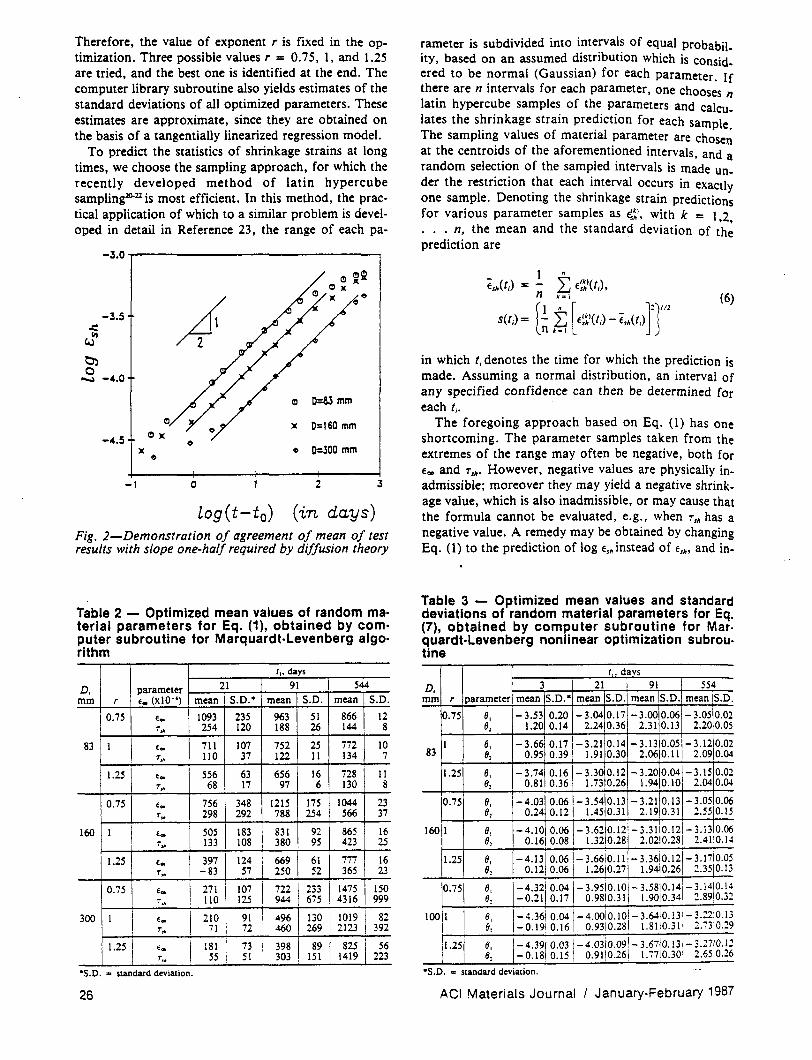
log(t-to) (in days) Fig. 2-Demonstration of agreement of mean of test results with slope one-half required by diffusion theory

Table 2 - Optimized mean values of random mao terial parameters for Eq. (1), obtained by com· puter subroutine for Marquardt·Levenberg algo· rithm

I,. days

D. parameter 21 91 544 mm r E. (x10-') mean S.D.· mean S.D. mean S.D.

0.75 E. 1093 235 963 51 866 12 T", 254 120 188 26 144 8

83 1 E. 711 107 752 25 772 10 T .. 110 37 122 11 134 7

1.25 E. 556 63 656 16 728 11 T .. 68 17 97 6 130 8

0.75 E. 756 348 1215 175 1044 23 T .. 298 292 788 254 566 37

160 1 I f. 505 183 831 92 865 16 T" 133 108 380 95 423 25

1.25 E.

1 397 124 669 61 777 16

T" -83 57 250 52 365 23

0.75 E. I

271 1

107 I 722 I 233

1

1475 !

150 T .. 110 125 944 675 4316 999

300 1 1

210 1 91 I ~I 130 i 1019 I 82 E.

I T" 71 72 269 2123 392

11.25 I E. I 181 1 73 I 398 I 89 825 [ 56

T" 55 51 I 303 , 151 1419 223

·S.O. a standard deviation.

26

rameter is subdivided into intervals of equal probabil_ ity, based on an assumed distribution which is Consid_ ered to be normal (Gaussian) for each parameter. If there are n intervals for each parameter, one chooses n latin hypercube samples of the parameters and calcu­lates the shrinkage strain prediction for each sample The sampling values of material parameter are chose~ at the centroids of the aforementioned intervals, and a random selection of the sampled intervals is made un­der the restriction ~hat each i?terval Occurs in exactly one sample. Denotmg the shnnkage strain predictions for various parameter samples as E.~l, with k = 1,2, . . . n, the mean and the standard deviation of the prediction are

(6)

in which ti denotes the time for which the prediction is made. Assuming a normal distribution, an interval of any specified confidence can then be determined for each ti'

The foregoing approach based on Eq. (1) has one shortcoming. The parameter samples taken from the extremes of the range may often be negative, both for fCD and "sh' However, negative values are physically in­admissible; moreover they may yield a negative shrink­age value, which is also inadmissible, or may cause that the formula cannot be evaluated, e.g., when "sh has a negative value. A remedy may be obtained by changing Eq. (1) to the prediction of log EShinstead of Esh , and in-

Table 3 - Optimized mean values and standard deviations of random material parameters for Eq. (7), obtained by computer subroutine for Mar· quardt·Levenberg nonlinear optimization subrou· tine

~davs

D. 3 21 91 1 554 mm r parameter mean S.D.· mean S.D. mean IS.D. mean S.D.

0.75 8, -3.53 0.20 -3.04 0.17 -3.00 0.06 - 3.0510.02 8, 1.20 0.14 2.24 0.36 2.31 0.13 2.2010.05

1 8, -3.66 0.17 -3.21 0.14 -3.13 0.05 -3.12 0.D2 83 8, 0.95 0.39 1.91 0.30 2.06 0.11 2.09 0.04

1.25 9, -3.74 0.16 -3.300.12 -3.200.04 -3.15 0.02 8, 0.8110.36 1.7310.26 1.9410.10 2.04 0.04

0.75 9, -4.03 0·061-3.5~10.\3 -3.210.13 -3.05 0.06 9, 0.24 0.12 1.4510.31 2.190.31 2.55 0.15

160 1 8, 1-4.10 0.06 - 3.6210.121- 3.3110.121- 3.13!0.06 9, 0.1610.08 1.3210.28 2.0210.281 2.41 0.14

1.25 9, -4.1310.06 -3.6610.11 -3.36jO.121-3.1~10.05 8, 0.12 0.06 1.2610.27 1.9410.26 2.350.13

1°.75\

8, -4.32\ 0.04!-3.9510.101-3.58io.141-3.1410.14 8, -0.21 0.17 0.9810.31 1.9010.34 2.89!0.32

8, 1-4.3610.041-4.0010.101-3.6410.131-3.2210.13 e, -0.19i 0.16 0.9310.281 1.8110.311 2.7310.29

-4.391' 0.031-4.03io.09!.-3.6710.!3i-3.27Io.1~ -0.18 0.15! 0.9110.261 1.7710.301 2.650.26

·S. O. " standard deviation.

ACI Materials Journal January-February 1987

troducing new parameters 81 and 82 which can take any real value. positive or negative. This is achieved by writing Eq. (1) in the form

log EM = 81 - ~ log [1 + C~f2)'] (7)

in which

-u Regrusion Analysis Da83 rnm -..... ---......... --; .

'" . .c: -u '" 0

'" 0

r.J'" , , 0 , 0

0 , ~ .... / .... ------I 0 I /' .... ". ,

'" '" /

~-/

1,.3 doys / / .... /

ti .... ~ ....

CI:l -u .... '---1,"91 doys , ".,.

~ ". ".

~ / ,

ti aU , /

...l.C , ~

I / ,

.~ .... / / / /

..:: I / / I

CI:l I / • Data_ I I ill..,. ..... I

/ o Dataoot_ I

/

... 0.75

/ I

I

I /

I I

/ I

I '"

" '" '" .,-

(8)

-­~~

1,.21 days

1,=554 day.~::::==: ..., ,

/

" "

---15li",'.1ImiI

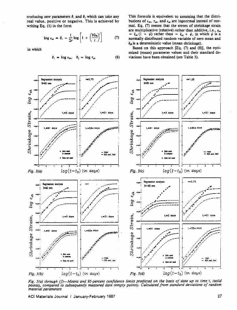
Fig.3(a) log(t-to) (in days)

-u

.c: -u III

r.J

~ ...... 0 ....

RegrlSsion Analysis 0=83 mm

r:sl _------".'

,,/ " 00-"_--,

//// /""'----, ,/ , ".

I I

/,,-------- 1/ //

'" I I / /

/ I /1 /

~- / 1,.3 days / 1,.21 days

.~ .... ~/_/----~--------~ ~/_I--------------~ ~ .....

CIJ -u

---. IS% C'IM. "mit

Fig.3(b) log(t-to) (in days)

This formula is equivalent to assuming that the distri­butions of Eoo. T,ir• and EM are lognormal instead of nor­mal. Eq. (7) means that the errors of shrinkage strain are multiplicative (relative) rather than additive. i.e., f,it

= EM (1 + 1/1) rather than = f,it + 1/1, in which 1/1 is a normally distributed random variable of zero mean and Ei/ris a deterministic value (mean shrinkage).

Based on this approach [Eq. (7) and (8)], the opti­mized (mean) parameter values and their standard de­viations have been obtained (see Table 3).

-u Regrlssion Analysis ... 1.25

D=83 mm -----0" ". .... -.-

00 ,,'" .. 0 , 0

.c: -u ""..,.,.-... ------ / III ".,. 0 I ..... .,,----

r.J '" 0 / , I 0 / , , , I /

~ / I , ..... / / I

0 ------- / ,.. I .... / / / I

'" / / I ..... / I / I

~- I 1,.3 days / 1,=21 days I I

/ / . ... I I

ti .... ~ ....

CI:l -u 1,.91 day. ----

~ " /" ,------~ / .-

-u , /

/ / ...l.C / , ~ "'/ I I

.~ ..... / ' I I /

, , , ~ / I

I ' ,

/ 7 • Data_ CI:l / I • - ..... ..... I illlIIIIyIiI ,/:,.;/ --15X",'.lImft / • I o Dolo 011_

-... -.j..,,-------~. -.j..,,-""!---~-~~ Fig.3(c) log(t-to) (in days)

-u Regression Analysis ... 0.75

~ o ....

aU

Fig.3(d)

0=160 mm

o •

... 0

0

•

log(t-to) (in days)

- mta1I - 15%,"".1imi1

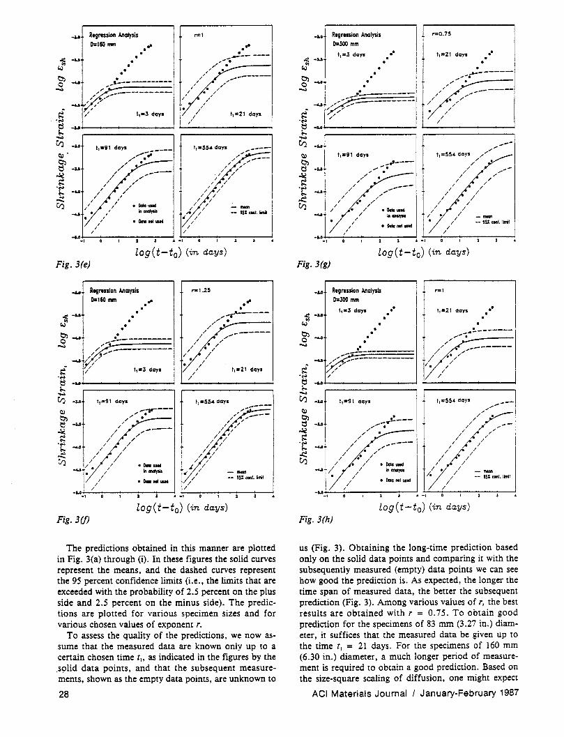
Fig. 3(a) through (f)-Means and 95-percent confidence limits predicted on the basis of data up to time tJ (solid points), compared to subsequently measured data (empty points). Calculated from standard deviations of random material parameters

ACI Materials Journal I January-February 1987 27

-1.1 Regreuion Ano/ysis r=1

0=160 mm . " .. . . . .c ..... . ,.,_..---- ---co ' .

'-l • ,/ . • , . . , /

~ / ------• , ", 0 ..... r=== , ,

-- , / ,

/ . , 6' ,,- , ,

// /"jI''' / , , ..... , ,

~-, ,

" 1,.3 days I 1,.21 day. / , ... , , 0 -u ~ ....

C/J -1.1 1,.91 days _----- 1,.55. day. ------Q). ;,,/ ... ",

, ~ /

/ " . /

0 -1.1 " ,

I

...!C / ,--- ./

~ /

" ,- /

/ / /

.~ , I ..... / / / / /

~ , I /

/ / I / /

C/J / • Data ... , /

I / / / --, inaMlysil ..... , ,. / -- 15% ... t. !mil

, , • / , • Data ...... / / /

/ /

-,,,-,,,,-~----~-~-.... --I:-,-~--!--~-~-'" log(t-to) (in da.ys)

Fig.3(e)

RegAsslon Analysis O:UO mm ." • •

l,a91 day.

I /

/ I

I ..... / . . /

I

/ /

.... -;r--­", . ,'" .~~-­

/

1/ /

/ /

I

/

/ /

" .... /

---• Data UIIcf

inaMlysil

• DoN""' ....

ra1.25

I -u_.,.,~~----~-~-'" ~-~-~-~-~-...

log(t-to) (in da.ys) Fig.3(f)

The predictions obtained in this manner are plotted in Fig. 3(a) through (i). In these figures the solid curves represent the means, and the dashed curves represent the 95 percent confidence limits (Le., the limits that are exceeded with the probability of 2.5 percent on the plus side and 2.5 percent on the minus side). The predic­tions are plotted for various specimen sizes and for various chosen values of exponent r.

To assess the quality of the predictions, we now as­sume that the measured data are known only up to a certain chosen time tit as indicated in the figures by the .sglid data points, and that the subsequent measure­ments, shown as the empty data points, are unknown to

28

..... Regression Analysis 0=300 mm

1,=3 day.

. . · .' .

r=0.75

1,=21 day.

• .' . .

-----------,'. ", ..... _---I , . • . ;/ --------

-4.1 .,.' _- ,/ ~""'---:==-=------- /// . ///'

,/ ,,"" /

.~ /" //

o .... ~--------------- ~_I--_--_------~ ~ .... C/J _ ...

/ /

1,,,,91 days

/ , ,

,

/ /

.. ----,-" . , . ,'"

/

/ .- // /

/

.... , --­,-

• Data .... ,­

• Data""' ..... /

I

/ /

,,,,,---1,=55. day. ",'"

/ /

/

/ I

I /

/

/ /

/

/ /

/

/

/ /

/

",

" / /

/

--",

,­,-

.-!5% ... t.limit

/ .... -.,.,-~'-~-~-~-~.-~,-~-~-------... log(t-to) (in da.ys)

Fig.3(g)

_... Regression Analysis 0:300 mm

~ ..... o --

1,.3 day •

.'

. • • . ·

.' .

-4.1 /~ ,:---------- -;?----" ... / ,

~- " " .... /

,...1

1,.21 day. .0 o .

/

// /

/.

/

/ /

/

_4~------­",,,, ._-----. ,,"

/ /

-----­,-

o .... ~-____ --__ - __ --~ ~------__ --__ --__ __ ~ .......

C/J _ ... 1,.91 day •

/ I

/ -4...1- /1

Fig. 3 (h)

/ /

/

", ",

/

.8 __ -...,..-,,-" .

1,=554 days

log(t-to) (in da.ys)

us (Fig. 3). Obtaining the long-time prediction based only on the solid data points and comparing it with the subsequently measured (empty) data points we can see how good the prediction is. As expected, the longer the time span of measured data, the better the subsequent prediction (Fig. 3). Among various values of r, the best results are obtained with r = 0.75. To obtain good prediction for the specimens of 83 mm (3.27 in.) diam­eter, it suffices that the measured data be given up to the time tl = 21 days. For the specimens of 160 mm (6.30 in.) diameter, a much longer period of measure­ment is required to obtain a good prediction. Based on the size-square scaling of diffusion, one might expect

ACI Materials Journal I January-February 1987

that I, = 4 x 21 days = 84 days would be sufficient. However, as is apparent from Fig. 3(d) through (f) measurements of a duration longer than 91 days are re­quired for the specimens of 160 mm diameter.

Aside from statistical predictions, the measured dia­grams confirm that the trend of shrinkage based on diffusion theory, which requires the initial shrinkage curve to be described by Eq. (3), is correct (Fig. 2). Ac­cording to this equation, the shrinkage curve in a log­log plot should be initially a straight line of slope ex­actly 0.5. All test data agree with this slope extremely well, except for some small deviation during the first few hours of shrinkage (for D == 83 mm) or the first day of shrinkage (for D = 160 mm). This deviation is probably due to the fact that the surface humidity of the cylinder does not become equal to the environmen­tal humidity instantly, as assumed in the determination of the exponent Y2 (see Appendix I), but with a delay due to a finite, rather than infinite, value of the mois­ture transmission coefficient at the surface. The shrinkage curves for the three specimen sizes are plot­ted together in Fig. 2, again making the straight-line slope of Yz conspicuous.

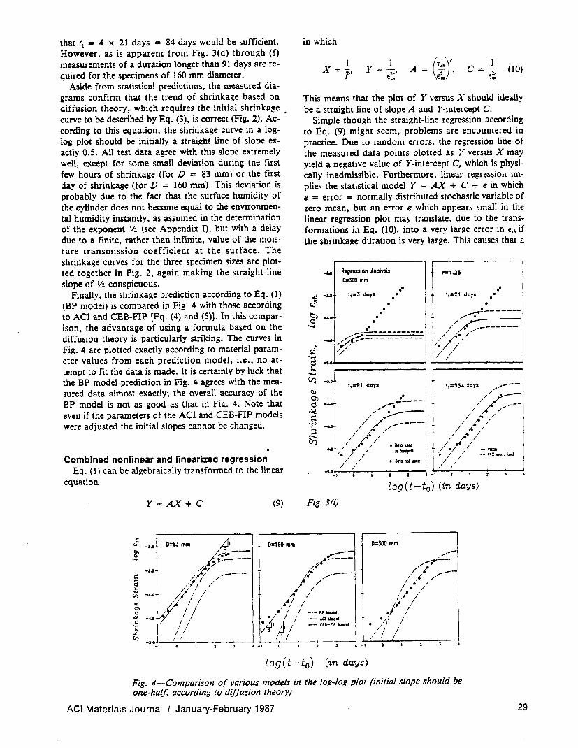
Finally, the shrin~age prediction according to Eq. (1) (BP model) is compared in Fig. 4 with those according to ACI and CEB-FIP {Eq. (4) and (5)]. In this compar­ison, the advantage of using a formula based on the diffusion theory is particularly striking. The curves in Fig. 4 are plotted exactly according to material param­eter values from each prediction model, i.e., no at­tempt to fit the data is made. It is certainly by luck that the BP model prediction in Fig. 4 agrees with the mea­sured data almost exactly; the overall accuracy of the BP model is not as good as that in Fig. 4. Note that even if the parameters of the ACI and CEB-FIP models were adjusted the initial slopes cannot be changed.

Combined nonlinear and linearized regression Eq. (1) can be algebraically transformed to the linear

equation

Y== AX+ C (9)

0=160 mill 'li 0=83 mm '" -1.0

0> .......... - .. -3

e ____

.---/// "" -u

i /,'/ / .-.--. ... "" t:l / /

in which

1 X ==-=,

f

1 C == - (10)

E~

This means that the plot of Y versus X should ideally be a straight line of slope A and Y-intercept C.

Simple though the straight-line regression according to Eq. (9) might seem, problems are encountered in practice. Due to random errors, the regression line of the measured data points plotted as Y versus X may yield a negative value of Y-intercept C, which is physi­cally inadmissible. Furthermore, linear regression im­plies the statistical model Y == AX + C + e in which e == error == normally distributed stochastic variable of zero mean, but an error e which appears small in the linear regression plot may translate, due to the trans­formations in Eq. (l0), into a very large error in Es~ if the shrinkage duration is very large. This causes that a

-. R'grusion Analysis 0=300 mm

o .' .

o o

.0 o

o o

o --.!------

,/'~ _~o ___ _

.- /~ ,,--------~- ~ r----::-----:----::: /:/ /;/ .~ -uJ-.. _______ ~ J...--..:/~ _____ ___<

~ .... rt:l

1,=91 day. 1,=554 day.

-1.1

/ -u / /

/ /

/ ~ /

/ 0

:(/ .... -,

Fig.3(i)

,..---­,,?----

Ii' I.t· /'-'-

J ./

/

/

00 ..-------,,~ 0

'" 0 / /

I -----.,. I .- / 0

/ / /

0 / / I / / / / • DGta .... / /

illOIIGIysiI

1 ' 0

/ / • DGta not .... /

I

- -, log(t-to) (in da.ys)

0=300 mm

,./,,-

-iI"-­""",

/.. _.---/.1 ,/

- mtGn .... 9~: =t\t. limit

/, ... / (;j ..... /, I ,of /

.~/ ! /

I / I • ,/ /. /

1./ ./ .. /, I 0> I t:l A I I "'I --05 ~ / i . ~ I .

.<:! I .I tIj

-5.0 I ,

-,

? I 1---81'.0001 0.' I / __ .aUodo'

~' j, ./ -- ctB-np _,

I I /

;'

--, - -,

log(t-to) (in da.ys)

Ie" / t / ., /

0/, I ,.; ,

/1 / / I i

Fig. 4-Comparison of various models in the log-log plot (initial slope should be one-half, according to diffusion theory)

ACI Materials Journal/January-February 1987 29

-...

C--3.12' ..... 0.021

- ... ,.1-_-•. -. --_"'Z .• ---,-.• --.• :---l .1-_-.. -. --_~Z .• ---,~ .• --.• :---l ---_""! •. ~. --_ .... Z .• ---,'"": .• ----' .• :---l

'000 -... 0= 83 mm 1 1,=21 days 0

s::100 /-.:.::. ,(eo

·S -;-. ..---

0 1.,// ... ~ <:1>- 'I 0-, ~ 0

~ '1:: zoo ~ Cr.I --• -, Fig.5(a)

-1.0

r=l ~ :fY/

/

y 0-0.5 ~ C--3.015

.. ?" '+10-0•072

1 w

'" .2 ..... 0 u

).,

1=-log [I +( r..llJJ

• DatI IIIOd io...,..

• DatI""_

log(t-to}

1,=91 days

.,--

d

,,{..-­ff/

(in days)

C--l.OIO .... aO.O.l

1,=554 days

0-0.5 . C __ l.ll7

," •• 0.102 /'

-I·~ ... O:-~-.~ .• --""!z.~. -_ .... , .• :---...... - ....... 0 -S.O -Z.O -1.0 .0 , .. -".0 -l.D -1.0 -1.0 .0

1=-log 11 +( r.w'WI '000

.I / -.. 1,=554 days ;., 1 0=160 mm 1,=21 days 1,=91 day. I 0

s:: "" /-

~ /1(; .:.::. / • DatI usod

.::; ... /0° 0 ioanalysis /, '7 0 I·

• Dolo not_ I /~ ;,1 ... ~

~ ; <:1>- /;./ ~ !. /--~ A,I / .S zoo ~"// ~jf! ~ 4"./

~ ~ ..... ---' • -~ -I . -, Fig.5(b) log( t-to} (in da.ys)

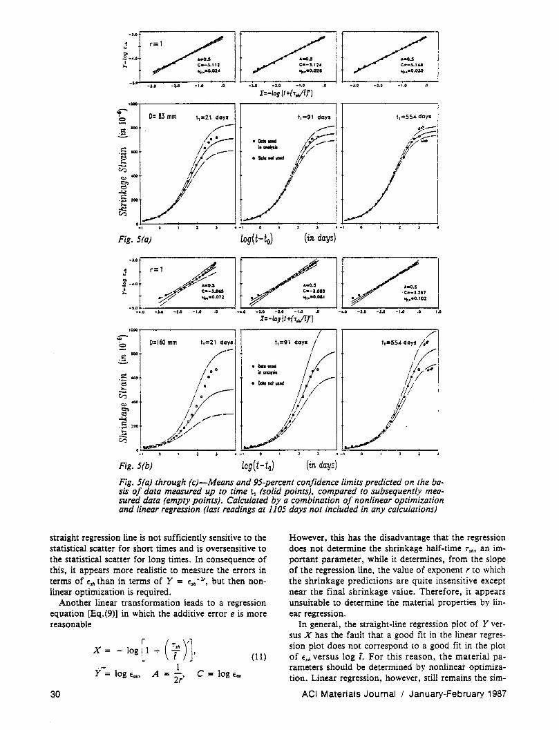
Fig. 5(a) through (c)-Means and 95-percent confidence limits predicted on the ba­sis of data measured up to time tl (solid points), compared to subsequently mea­sured data (empty points). Calculated by a combination of nonlinear optimization and linear regression (last readings at 1105 days not included in any calculations)

straight regression line is not sufficiently sensitive to the statistical scatter for short times and is oversensitive to the statistical scatter for long times. In consequence of this, it appears more realistic to measure the errors in terms of E.h than in terms of Y = E.h -lr, but then non­linear optimization is required.

However, this has the disadvantage that the regression does not determine the shrinkage half-time Trn , an im­portant parameter, while it determines, from the slope of the regression line, the value of exponent r to which the shrinkage predictions are quite insensitive except near the final shrinkage value. Therefore, it appears unsuitable to determine the material properties by lin­ear regression.

Another linear transformation leads to a regression equation [Eq.(9)] in which the additive error e is more reasonable

Y = log E.n,

30

A=-2r'

(11)

C = log E ..

In general, the straight-line regression plot of Y ver­sus X has the fault that a good fit in the linear regres­sion plot does not correspond to a good fit in the plot of Ern versus log i. For this reason, the material pa­rameters should be determined by nonlinear optimiza­tion. Linear regression, however, still remains the sim-

ACI Materials Journal I January-February 1987

-J.O

r=l d 4--

-"'" ...... ~ V •• O.5 -- /' C--2.tl2

/' ~,.-O.I05 -s.O

-".0 -J.O -2.0 -1.0 .0 -".0 -J.O -2.0 -1.0 .0

.·o.~ C--l.I78 ,+.-0.145

..... 0 -.J.O -LO -1.0 .0

X=-log(f+(T.lm .*r-----------------~ r----------------~ r---------------,-~

vr 0=300 mm 8 I.. 1,=21 days

.:; -

-.

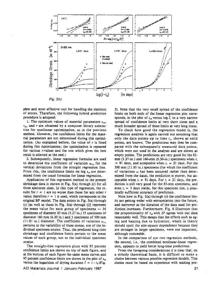
Fig.5(c)

• Dat._ ... naIpiI

• Dat ... tuud

pI est and most effective tool for handling the statistics of errors. Therefore, the following hybrid prediction procedure is adopted:

1. The optimum values of material parameters f oo ,

1',h' and r are obtained by a computer library subrou­tine for nonlinear optimization, as in the previous method. However, the confidence limits for the mate­rial parameters are not determined during this optimi­zation. (As explained before, the value of r is fixed during this optimization; the optimization is repeated for various r-values and the one which gives the best result is selected at the end.)

2. Subsequently, linear regression formulas are used to determine the coefficient of variation WYlx for the vertical deviations from the straight regression line. From this. the confidence limits on log ~sh are deter­mined from the usual formulas for linear regression.

Application of this regression method to the present shrinkage data is shown in Fig. Sea) through (c) for all three specimen sizes. In this type of regression, the re­sults for r = 1 are no worse than those for any other r value; therefore r = 1 is used, which corresponds to the original BP model. The data points in Fig. 5{a) through (c) [as well as those in Fig. 3(a) through (i)] represent the mean value for each group of specimens - 36 specimens of diameter 83 mm (3.27 in.) 35 specimens of diameter 160 mm (6.30 in.) and 3 specimens of 300 mm (11. 81 in.) diameter. The coefficient of variation Wyl.

pertains to the variability of these means, not of the in­dividual specimen strains. Thus, the predicted long-time shrinkage and confidence limits pertain to the mean values of each group, not to the individual specimen strains.

The straight-line regression plots with 95 percent confidence limits are shown on top of each figure, and at the bottom of each figure the same mean curves and 95 percent confidence limits are shown in the plot of fsh

versus the logarithm of drying duration f = t - to (Fig.

ACI Materials Journal I January-February 1987

(in da.ys)

5). Note that the very small spread of the confidence limits on both ends of the linear regression plot corre­sponds, in the plot of €'h versus log f, to a very narrow spread of confidence limits at very short times and a much broader spread of these limits at very long times.

To check how good the regression model is, the regression analysis is again carried out assuming that only the data points up to time t l , shown as solid points, are known. The predictions may then be com­pared with the subsequently measured data points, which were not used in the analysis and are shown as empty points. The predictions are very good for the 83-mm (3.27-in.) and 160-mm (6.30-in.) specimens when tl

= 91 days, and acceptable when tl = 21 days. For the 300 mm (11.81 in.) specimens (for which the coefficient of variations W has been assumed rather than deter­mined from the data). the prediction is poorer, but ac­ceptable when tl = 91 days. For tl = 21 days. the pre­diction is still very good for the 83-mm specimens, and even t, = 3 days yields, for this specimen size, a prac­tically sufficient accuracy of prediction.

Note how in Fig. Sea) through (c) the confidence lim­its are gettmg wider with extrapolation into the future, and narrower as the duration of the data used for pre­diction increases. Furthermore, Fig. 6 illustrates that the proportionality of T.h with IJ2 agrees with our data reasonably well. This means that the effects such as ag­ing and heating due to hydration, which in theory should spoil the size-square dependence because they are stronger in larger specimens, were not important, although noticeable.

In the comparison of our two regression methods, the second, i.e .• the combined nonlinear-linear regres­sion, appears to yield better long-time predictions.

From the foregoing considerations it is clear that. on a strictly theoretical basis, it is difficult to make a choice between various possible regression models. This choice must be based on experience with making pre-

31

- r=l c.=753xl0-' 'To= 1.326x 1 0-2

-1.0 -~ .0 .5 '.G ,-' 2.D

log(Hol

... --.---------~:--.-. ... -.- .

.11

2-' l.D l--' 4.0 4.'

(in days)

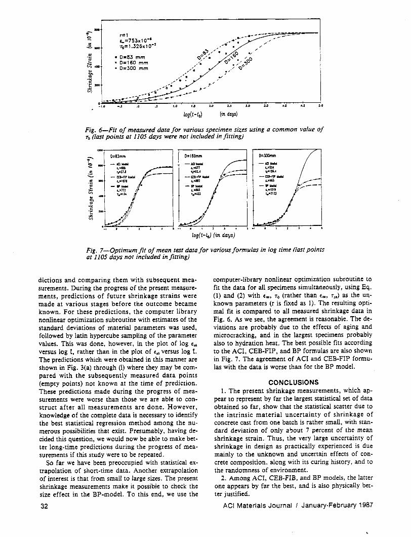
Fig. 6-Fit of measured data for various specimen sizes using a common value of To (last points at 1105 days were not included in fitting)

,-::-- O=83mm O=160mm O=300mm

~ - -oID_ -oID_ --oID_ 1.:6" c.-617 .. ~

s:: 1"Z7.I 1",1.4 ..... 121.( .:::.. - C[8-np_ -t[8-nP_

05 ... c.a l01 • .. _w /,----<:! -11'- -er_ 0/ _-.t; c,.wnz c.alOt'

~ ...... V:l r.zU4 ,,-Z'll co -."

'" .l ... r:: ... or'

~ AI .(.1

<f"

• -, log(Ho) (in days)

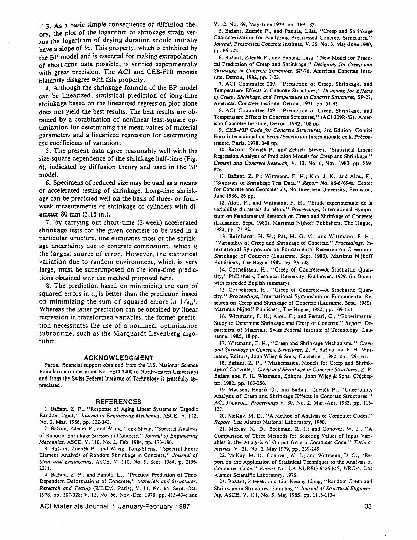
Fig. 7-0ptimum fit of mean test data for various formulas in log time (last points at 1105 days not included in fitting)

dictions and comparing them with subsequent mea­surements. During the progress of the present measure­ments, predictions of future shrinkage strains were made at various stages before the outcome became known. For these predictions, the computer library nonlinear optimization subroutine with estimates of the standard deviations of material parameters was used, followed by latin hypercube sampling of the parameter values. This was done, however, in the plot of log E,. versus log i, rather than in the plot of E,. versus log t The predictions which were obtained in this manner are shown in Fig. 3(a) through (i) where they may be com­pared with the subsequently measured data points (empty points) not known at the time of prediction. These predictions made during the progress of mea­surements were worse than those we are able to con­struct after all measurements are done. However, knowledge of the complete data is necessary to identify the best statistical regression method among the nu­merous possibilities that exist. Presumably, having de­cided this question, we would now be able to make bet­ter long-time predictions during the progress of mea­surements if this study were to be repeated.

So far we have been preoccupied with statistical ex­trapolation of short-time data. Another extrapolation of interest is that from small to large sizes. The present shrinkage measurements make it possible to check the size effect in the BP-model. To this end, we use the

32

computer-library nonlinear optimization subroutine to fit the data for all specimens simultaneously, using Eq. (1) and (2) with EOD , To (rather than EOD , T,.) as the un­known parameters (r is fixed as 1). The resulting opti­mal fit is compared to all measured shrinkage data in Fig. 6. As we see, the agreement is reasonable. The de­viations are probably due to the effects of aging and microcracking, and in the largest specimens probably also to hydration heat. The best possible fits according to the ACI, CEB-FIP, and BP formulas are also shown in Fig. 7. The agreement of ACI and CEB-FIP formu­las with the data is worse than for the BP model.

CONCLUSIONS 1. The present shrinkage measurements, which ap­

pear to represent by far the largest statistical set of data obtained so far, show that the statistical scatter due to the intrinsic material uncertainty of shrinkage of concrete cast from one batch is rather small, with stan­dard deviation of only a 'Jout 7 percent of the mean shrinkage strain. Thus, the very large uncertainty of shrinkage in design as practically experienced is due mainly to the unknown and uncertain effects of con­crete composition, along with its curing history, and to the randomness of environment.

2. Among ACI, CEB-FIB, and BP models, the latter one appears by far the best, and is also physically bet­ter justified.

ACI Materials Journal I January-February 1987

· 3. As a basic simple consequence of diffusion the­ory, the plot of the logarithm of shrinkage strain ver­sus the logarithm of drying duration should initially have a slope of V2. This property, which is exhibited by the BP model and is essential for making extrapolation of short-time data possible, is verified experimentally with great precision. The ACI and CEB-FIB models blatantly disagree with this property.

4. Although the shrinkage formula of the BP model can be linearized, statistical prediction of long-time shrinkage based on the linearized regression plot alone does not yield the best results. The best results are ob­tained by a combination of nonlinear least-square op­timization for determining the mean values of material parameters and a linearized regression for determining the coefficients of variation.

5. The present data agree reasonably well with the size-square dependence of the shrinkage half-time (Fig. 6), indicated by diffusion theory and used in the BP model.

6. Specimens of reduced size may be used as a means of accelerated testing of shrinkage. Long-time shrink­age can be predicted well on the basis of three- or four­week measurements of shrinkage of cylinders with di­ameter 80 mm (3.15 in.).

7. By carrying out short-time (3-week) accelerated shrinkage tests for the given concrete to be used in a particular structure, one eliminates most of the shrink­age uncertainty due to concrete composition, which is the largest source of error. However, the statistical variation due to random environment, which is very large, must be superimposed on the long-time predic­tions obtained with the method proposed here.

8. The prediction based on minimizing the sum of squared errors in Esh is better than the prediction based on minimizing the sum of squared errors in 11 fsh 2•

Whereas the latter prediction can be obtained by linear regression in transformed variables, the former predic­tion necessitates the use of a nonlinear optimization subroutine, such as the Marquardt-Levenberg algo­rithm.

ACKNOWLEDGMENT Partial financial support obtained from the U.S. National Science

Foundation (under grant No. FED 7400 to Northwestern University) and from the Swiss Federal Institute of Tec~nology is gratefully ap­preciated.

REFERENCES I. BaZant. Z. P., "Response of Aging Linear Systems to Ergodic

Random Input," Journal of Engineering MechaniCS, ASCE, V. 112, No.3, Mar. 1986, pp. 322-342.

2. BaZant, Zdenek P., and Wang, Tong-Sheng, "Spectral Analysis of Random Shrinkage Stresses in Concrete,'" Journal of Engineering Mechanics, ASCE, V. 110, No.2, Feb. 1984, pp. 173-186.

3. Bazant, Zdenek P., and Wang, Tong-Sheng, "Spectral Finite Element Analysis of Random Shrinkage in Concrete," Journal of Structural Engineering, ASCE, V. 110, No.9, Sept. 1984, p. 2196-2211.

4. BaZan!, Z. P., and Panula, L., "Practicl'l Prediction of Time­Dependent Deformations of Concrete," Materials and Structures, Research and Testing (RILEM, Paris), V. II, No. 65, Sept.-Oct. 1978, pp. 307-328; V. 11, No. 66, Nov.-Dec. 1978, pp. 415-434; and

ACI Materials Journal I January-February 1987

V. 12, No. 69, May-June 1979, pp. 169-183. 5. BaZant, Zdenek P., and Panula, Liisa, "Creep and Shrinkage

Characterization for Analyzing Prestressed Concrete Structures," Journal. Prestressed Concrete Institute, V. 25, No.3, May-June 1980, pp.86-122.

6. BaZant, Zdenek P., and Panula, Liisa, "New Model for Practi­cal Prediction of Creep and Shrinkage," Designing for Creep and Shrinkage in Concrete Structures. SP-76. American Concrete Insti­tute, Detroit, 1982, pp. 7-23.

7. ACI Committee 209, "Prediction of Creep, Shrinkage, and Temperature Effects in Concrete Structures," Designing for Effects of Creep. Shrinkage. and Temperature in Concrete Structures. SP-27, American Concrete Institute, Detroit, 1971, pp. 51-93.

8. ACI Committee 209, "Prediction of Creep, Shrinkage, and Temperature Effects in Concrete Structures," (ACI 209R-82), Amer­ican Concrete Institute, Detroit, 1982, 108 pp.

9. CEB-FIP Code jor Concrete Structures. 3rd Edition, Comite Euro-International du Beton/Federation Internationale de la Precon­trainte, Paris. 1978, 348 pp.

10. Bdant, Zden~k P., and Zebich, Steven, "Statistical Linear Regression Analysis of Prediction Models for Creep and Shrinkage," Cement and Concrete Research. V. 13, No.6, Nov. 1983, pp. 869-876.

II. BaZant, Z. P.; Wittmann, F. H.; Kim, J. K.; and Alou, F., "Statistics of Shrinkage Test Data," Report No. 86-6/694s, Center for Concrete and Geomaterials, Northwestern University, Evanston, June 1986, 26 pp.

12. Alou, F., and Wittmann, F. H., "Etude experimentale de la variabilite du retrait du beton," Proceedings, International Sympo­sium on Fundamental Research on Creep and Shrinkage of Concrete (Lausanne, Sept. 1980), Martinus Nijhoff Publishers, The Hague, 1982, pp. 75-92.

13. Reinhardt, H. W.; Pat, M. G. M.; and Wittmann, F. H., "Variability of Creep and Shrinkage of Concrete," Proceedings. In­ternational Symposium on Fundamental Research on Creep and Shrinkage of Concrete (Lausanne, Sept. 1980), Martinus Nijhoff Publishers, The Hague, 1982, pp. 95-108.

14. Cornelissen, H., "Creep of Concrete-A Stochastic Quan­tity," PhD thesis, Technical University, Eindhoven, 1979. (in Dutch, with extended English summary)

15. Cornelissen, H., "Creep of Concrete-A Stochastic Quan­tity," Proceedings. International Symposium on Fundamental Re­search on Creep and Shrinkage of Concrete (Lausanne, Sept. 1980), Martinus Nijhoff Publishers, The Hague, 1982, pp. 109-124.

16. Wittmann, F. H.; Alou, F.; and Ferrari, C., "Experimental Study to Determine Shrinkage and Creep of Concrete," Report, De­partment of Materials, Swiss Federal Institute of Technology, Lau­sanne, 1985, 18 pp.

17. Wittmann, F. -H., "Creep and Shrinkage Mechanisms," Creep and Shrinkage in Concrete Structures. Z. P. BaZanl and F. H. Witt­mann, Editors, John Wiley & Sons, Chichester, 1982, pp. 129-161-

18. BaZant, Z. P., "Mathematical Models for Creep and Shrink­age of Concrete," Creep and Shrinkage in Concrete Structures. Z. P. BaZant and F. H. Wittmann, Editors, John Wiley & Sons, Chiches­ter, 1982, pp. 163-256.

19. Madsen, Henrik 0., and Bdant, Zden~k P., "Uncertainty Ana:ysis of Creep and Shrinkage Effects in Concrete Structures," ACI JOURNAL, Proceedings V. 80, No.2, Mar.-Apr. 1983, pp. 116-127.

20. McKay, M. D., "A Method of Analysis of Computer Codes," Report. Los Alamos National Laboratory, 1980.

21. McKay, M. D.; Beckman, R. J.; and Conover, W. J., "A Comparison of Three Methods for Selecting Values of Input Vari­ables in the Analysis of Output from a Computer Code," Techno­metrics, V. 21, No.2, May 1979, pp. 239-245.

22. McKay, M. D.; Conover, W. J.; and Wittmann, D. C., "Re­port on the Application of Statistical Techniques to the Analysis of Computer Code," Report No. LA-NUREG-6526-MS, NRC-4, Los Alamos Scientific Laboratory, 1976.

23. BaZant, Zdenek, and Liu, Kwang-Liang, "Random Creep and Shrinkage in Structures: Sampling," Journal oj Structural Engineer­ing. ASCE, V. Ill, No.5, May 1985, pp. 1113-1134.

33

APPENDIX I - Some consequences of diffusion theory

Let us calculate from nonlinear diffusion theory the initial shape of the shrinkage curve. At the beginning of drying, the drying front moves from the surface into the specimen. For short times, the pen­etration depth of the drying front 0 is small compared to the curva­ture radius of the surface R which means that initially the drying can be treated as a penetration of the drying front from the surface into a halfspace. The pore relative humidity is initially unifonn, h = h., and it is assumed that at the time I. the pore humidity at the surface drops instantly by Ah = h. - ho where h. = environmental relative hu­midity. Neglecting self-desiccation due to hydration and the effect of aging (hydration), the diffusion equation in one dimension may be written as

ah .. k~ (c Oh) 01 ox ax

(12)

in which x = depth coordinate (distance from the surface), C = penneability, and k .. slope of the desorption isothenn. Coefficients c and k arc functions of pore humidity h.

We now assume the pore humidity distributions at various times to be given as

Ah .. 1m, ~ .. x/6(1) (13)

in which 1m is a certain function giving the shape of the humidity profile, and 0(1) is a drying penetration depth at time 1 such that h .. h. for x > 0 (I). The flux of water from the halfspace surface may be expressed as

d r"'" d r' J .. - dr J. F(Ah)dx = -dr J, FVWI d~ 0(1) = -c,6(1) (14)

in which F(Ah) is the specific water content of concrete (kg per m'); function F(.a.h) defines the desorption isotherm. Assuming the hu­midity profile shapes flE) to be the same for all times, the last inte­gral in Eq. (14) is a constant, denoted as c,. The flux of water from the surface may be also expressed as

J = -c[grad hI, .... -c[o(Ah)/ox)zo' = -cf'(O)/o(l) (15)

= - C/O(I)

in which c, .. c!' (0) .. constant if the humidity profile shape re­mains constant. Equating our two expressions for J, we have 260" Co in which c ... 2c,l C, = constant. This is a differential equation for 0, the solution of which is

0(1) = [c.(t-I,»)'" (16)

It remains to check that the humidity profile indeed keeps the same shape, as assumed. To this end, we substitute Eq. (13) into Eq. (12),

which after rearrangements and substitution 60 = c.12 yields the differential equation

(17)

The coefficients of this differential equation are time-independent, as is the boundary condition. Hence the solution fl~) is time-inde­pendent, which proves our assumption.

We know that, as a rather good approximation at the beginning, the shrinkage strain may be considered proportional to the total wa­ter loss W from the specimen. Thus, we may caiculate

34

E .. = k.W = k. r F(Ah)dx= k.o(t) i: FUm)d~ = k,k, 0 (I) (18)

in which the last integral is a constant, denoted as k,. Now, substitut­ing Eq. (16), we finally obtain for the initial period of drying

E .. = [k,,(1 - t.)I~ (19)

in which k. = c. k; k,' = constant. This proves that the initial shape of the plot of log E .. versus log (I - I.) should be a straight line of slope Yl, as is verified by the present tests. This property has been known for the linear diffusion theory, however, for concrete it is important that this property also holds for nonlinear diffusion theory.

APPENDIX" - Some other shrinkage formulas Aside from Eq. (I), other simple formulas exist which exhibit the

square-root type time-dependence [Eq. (4») at early times

- (I -';""'~')' E ... - E. - e (20)

E .. = E. [tanh (fJr (21)

E, • = E~ [; arctan (~)'r (22)

These formulas, however, differ from EQ. (I) in the long-time asymptotic behavior. For i - 00, EQ. (I), (20), (21) and (22) asymp­totically approach the formulas

E I (E.,]' for Eq. (I): - = 1 - - -E. 2r 1 (23)

for Eq. (20): .!.. = 1 -~iIT .. I'II' - re (24) E.

for Eq. (21): .!.. .. 1 _! e·ZlilT,lIf (25) E. r

for EQ. (22): .!.. = 1 (T .. )' (26) 1-- -E. 'II'r I

Now, which asymptotic behavior is more realistic? According to the linear diffusion theory, i.e., for constant diffusivity, the total water loss W from the specimen approaches th~ final state like a decaying exponential. This happens to be true for EQ. (24) and (25) for r .. I. However, in reality the diffusion equation for water in concrete is nonlinear, with the diffusivity strongly decreasing at a decreasing hu­midity. Therefore, the approach to the final state should be slower than that of a decaying exponential, which means that the function (I - E .. I E.) Ie·;' should be an inc:-easing function of time; this is the case for the inverse (decaying) power functic..ns in Eq. (23) and (26). For Eq. (24) and (25) the approach to the final state seems to be too fast. Consequently, among Eq. (I), (20), (21) and (22), a more real­istic asymptotic behavior seems to be exhibited by Eq. (I) and EQ. (22). It should be pointed out, however, that contrary to the initial shrinkage the long-time asymptotic behavior cannot be checked by experimental findings at this moment.

All the fonnulas in Eq. (20), (21), and (22) have been tried, but none offered any better representation of the present data than EQ. (1) used in the BP model. Numerous other formulas for shrinkage have been proposed in the past, but we need not elaborate on them because their initial behavior contradicts the diffusion theory.

ACI Materials Journal I January February 19b7