AcknowledgementsThis tutorial was created for Yang Xu’s Data Science and The Mind course (COGSCI 88, spring, 2016) at UC Berkeley.Thank you to Yang for spending many hours going over the structure and format of this tutorial, as well as VasilisOikonomou and Elva Xinyi Chen for providing helpful comments and revisions.

1

Contents

1 Getting started 41.1 Overview . . . . . . . . . . . . . . . . . . . . . . . . . . . . . . . . . . . . . . . . . . . . . . . . . . . . . . 41.2 Installation . . . . . . . . . . . . . . . . . . . . . . . . . . . . . . . . . . . . . . . . . . . . . . . . . . . . . 51.3 Running Python . . . . . . . . . . . . . . . . . . . . . . . . . . . . . . . . . . . . . . . . . . . . . . . . . . 5

1.3.1 From a Jupyter notebook . . . . . . . . . . . . . . . . . . . . . . . . . . . . . . . . . . . . . . . . . 51.3.2 From the command line . . . . . . . . . . . . . . . . . . . . . . . . . . . . . . . . . . . . . . . . . . 6

1.4 An example . . . . . . . . . . . . . . . . . . . . . . . . . . . . . . . . . . . . . . . . . . . . . . . . . . . . . 6

2 Data Structures 82.1 List . . . . . . . . . . . . . . . . . . . . . . . . . . . . . . . . . . . . . . . . . . . . . . . . . . . . . . . . . 8

2.1.1 Basic operations . . . . . . . . . . . . . . . . . . . . . . . . . . . . . . . . . . . . . . . . . . . . . . 82.1.1.1 Accessing an element in a list . . . . . . . . . . . . . . . . . . . . . . . . . . . . . . . . . . 82.1.1.2 Accessing parts of a list . . . . . . . . . . . . . . . . . . . . . . . . . . . . . . . . . . . . . 92.1.1.3 Iterating over a list . . . . . . . . . . . . . . . . . . . . . . . . . . . . . . . . . . . . . . . 92.1.1.4 Obtaining a random element from a list . . . . . . . . . . . . . . . . . . . . . . . . . . . . 92.1.1.5 Randomizing a list . . . . . . . . . . . . . . . . . . . . . . . . . . . . . . . . . . . . . . . . 92.1.1.6 Reversing indices . . . . . . . . . . . . . . . . . . . . . . . . . . . . . . . . . . . . . . . . . 92.1.1.7 List comprehension . . . . . . . . . . . . . . . . . . . . . . . . . . . . . . . . . . . . . . . 102.1.1.8 Reversing a list . . . . . . . . . . . . . . . . . . . . . . . . . . . . . . . . . . . . . . . . . . 10

2.1.2 Visualization . . . . . . . . . . . . . . . . . . . . . . . . . . . . . . . . . . . . . . . . . . . . . . . . 102.1.2.1 Pie chart . . . . . . . . . . . . . . . . . . . . . . . . . . . . . . . . . . . . . . . . . . . . . 102.1.2.2 Scatter plot . . . . . . . . . . . . . . . . . . . . . . . . . . . . . . . . . . . . . . . . . . . . 112.1.2.3 Bar plot . . . . . . . . . . . . . . . . . . . . . . . . . . . . . . . . . . . . . . . . . . . . . . 11

2.1.3 Further readings . . . . . . . . . . . . . . . . . . . . . . . . . . . . . . . . . . . . . . . . . . . . . . 112.2 Array . . . . . . . . . . . . . . . . . . . . . . . . . . . . . . . . . . . . . . . . . . . . . . . . . . . . . . . . 11

2.2.1 Basic operations . . . . . . . . . . . . . . . . . . . . . . . . . . . . . . . . . . . . . . . . . . . . . . 122.2.1.1 Taking the logarithm . . . . . . . . . . . . . . . . . . . . . . . . . . . . . . . . . . . . . . 122.2.1.2 Taking the absolute value . . . . . . . . . . . . . . . . . . . . . . . . . . . . . . . . . . . . 132.2.1.3 Taking the mean of a single array . . . . . . . . . . . . . . . . . . . . . . . . . . . . . . . 132.2.1.4 Taking the mean of multiple arrays . . . . . . . . . . . . . . . . . . . . . . . . . . . . . . 132.2.1.5 Operating over multiple arrays . . . . . . . . . . . . . . . . . . . . . . . . . . . . . . . . . 142.2.1.6 Converting arrays to lists . . . . . . . . . . . . . . . . . . . . . . . . . . . . . . . . . . . . 142.2.1.7 Converting lists to arrays . . . . . . . . . . . . . . . . . . . . . . . . . . . . . . . . . . . . 14

2.2.2 Visualization . . . . . . . . . . . . . . . . . . . . . . . . . . . . . . . . . . . . . . . . . . . . . . . . 142.2.2.1 Histogram . . . . . . . . . . . . . . . . . . . . . . . . . . . . . . . . . . . . . . . . . . . . 142.2.2.2 Scatter plot . . . . . . . . . . . . . . . . . . . . . . . . . . . . . . . . . . . . . . . . . . . . 152.2.2.3 Log-log Plot . . . . . . . . . . . . . . . . . . . . . . . . . . . . . . . . . . . . . . . . . . . 15

2.2.3 Further readings . . . . . . . . . . . . . . . . . . . . . . . . . . . . . . . . . . . . . . . . . . . . . . 152.3 Dictionary . . . . . . . . . . . . . . . . . . . . . . . . . . . . . . . . . . . . . . . . . . . . . . . . . . . . . . 15

2.3.1 Basic operations . . . . . . . . . . . . . . . . . . . . . . . . . . . . . . . . . . . . . . . . . . . . . . 162.3.1.1 Indexing . . . . . . . . . . . . . . . . . . . . . . . . . . . . . . . . . . . . . . . . . . . . . 162.3.1.2 Hashing . . . . . . . . . . . . . . . . . . . . . . . . . . . . . . . . . . . . . . . . . . . . . . 162.3.1.3 Key-value pairing . . . . . . . . . . . . . . . . . . . . . . . . . . . . . . . . . . . . . . . . 162.3.1.4 Using a dictionary . . . . . . . . . . . . . . . . . . . . . . . . . . . . . . . . . . . . . . . . 172.3.1.5 Sorting values in a dictionary . . . . . . . . . . . . . . . . . . . . . . . . . . . . . . . . . . 17

2.3.2 Further readings . . . . . . . . . . . . . . . . . . . . . . . . . . . . . . . . . . . . . . . . . . . . . . 172.4 Pandas . . . . . . . . . . . . . . . . . . . . . . . . . . . . . . . . . . . . . . . . . . . . . . . . . . . . . . . . 17

2.4.1 Basic operations . . . . . . . . . . . . . . . . . . . . . . . . . . . . . . . . . . . . . . . . . . . . . . 182.4.1.1 Averaging . . . . . . . . . . . . . . . . . . . . . . . . . . . . . . . . . . . . . . . . . . . . . 182.4.1.2 Standard deviation . . . . . . . . . . . . . . . . . . . . . . . . . . . . . . . . . . . . . . . 182.4.1.3 Conversion to arrays . . . . . . . . . . . . . . . . . . . . . . . . . . . . . . . . . . . . . . . 19

2.4.2 Further readings . . . . . . . . . . . . . . . . . . . . . . . . . . . . . . . . . . . . . . . . . . . . . . 19

2

3 Tools 203.1 Statements . . . . . . . . . . . . . . . . . . . . . . . . . . . . . . . . . . . . . . . . . . . . . . . . . . . . . 20

3.1.1 import statement . . . . . . . . . . . . . . . . . . . . . . . . . . . . . . . . . . . . . . . . . . . . . . 203.1.2 for loop . . . . . . . . . . . . . . . . . . . . . . . . . . . . . . . . . . . . . . . . . . . . . . . . . . . 203.1.3 if statement . . . . . . . . . . . . . . . . . . . . . . . . . . . . . . . . . . . . . . . . . . . . . . . . . 203.1.4 while statement . . . . . . . . . . . . . . . . . . . . . . . . . . . . . . . . . . . . . . . . . . . . . . . 21

3.2 Functions . . . . . . . . . . . . . . . . . . . . . . . . . . . . . . . . . . . . . . . . . . . . . . . . . . . . . . 213.2.1 Creating a function . . . . . . . . . . . . . . . . . . . . . . . . . . . . . . . . . . . . . . . . . . . . . 213.2.2 Built-in functions . . . . . . . . . . . . . . . . . . . . . . . . . . . . . . . . . . . . . . . . . . . . . . 22

3.2.2.1 random.choice() . . . . . . . . . . . . . . . . . . . . . . . . . . . . . . . . . . . . . . . . . 223.2.2.2 random.shuffle . . . . . . . . . . . . . . . . . . . . . . . . . . . . . . . . . . . . . . . . . . 223.2.2.3 reversed() . . . . . . . . . . . . . . . . . . . . . . . . . . . . . . . . . . . . . . . . . . . . . 223.2.2.4 print() . . . . . . . . . . . . . . . . . . . . . . . . . . . . . . . . . . . . . . . . . . . . . . 233.2.2.5 sorted() . . . . . . . . . . . . . . . . . . . . . . . . . . . . . . . . . . . . . . . . . . . . . . 233.2.2.6 .append() . . . . . . . . . . . . . . . . . . . . . . . . . . . . . . . . . . . . . . . . . . . . . 243.2.2.7 .capitalize() . . . . . . . . . . . . . . . . . . . . . . . . . . . . . . . . . . . . . . . . . . . . 243.2.2.8 .lower() . . . . . . . . . . . . . . . . . . . . . . . . . . . . . . . . . . . . . . . . . . . . . . 243.2.2.9 .split() . . . . . . . . . . . . . . . . . . . . . . . . . . . . . . . . . . . . . . . . . . . . . . 24

3.3 Numpy and Scipy . . . . . . . . . . . . . . . . . . . . . . . . . . . . . . . . . . . . . . . . . . . . . . . . . . 253.3.1 Functions . . . . . . . . . . . . . . . . . . . . . . . . . . . . . . . . . . . . . . . . . . . . . . . . . . 25

3.3.1.1 absolute() . . . . . . . . . . . . . . . . . . . . . . . . . . . . . . . . . . . . . . . . . . . . . 253.3.1.2 arange() . . . . . . . . . . . . . . . . . . . . . . . . . . . . . . . . . . . . . . . . . . . . . . 253.3.1.3 array() . . . . . . . . . . . . . . . . . . . . . . . . . . . . . . . . . . . . . . . . . . . . . . 253.3.1.4 linspace() . . . . . . . . . . . . . . . . . . . . . . . . . . . . . . . . . . . . . . . . . . . . . 253.3.1.5 log() . . . . . . . . . . . . . . . . . . . . . . . . . . . . . . . . . . . . . . . . . . . . . . . . 253.3.1.6 .mean() . . . . . . . . . . . . . . . . . . . . . . . . . . . . . . . . . . . . . . . . . . . . . . 263.3.1.7 .sum() . . . . . . . . . . . . . . . . . . . . . . . . . . . . . . . . . . . . . . . . . . . . . . . 263.3.1.8 .tolist() . . . . . . . . . . . . . . . . . . . . . . . . . . . . . . . . . . . . . . . . . . . . . . 26

3.3.2 Matplotlib . . . . . . . . . . . . . . . . . . . . . . . . . . . . . . . . . . . . . . . . . . . . . . . . . . 263.3.2.1 bar() . . . . . . . . . . . . . . . . . . . . . . . . . . . . . . . . . . . . . . . . . . . . . . . 263.3.2.2 pie() . . . . . . . . . . . . . . . . . . . . . . . . . . . . . . . . . . . . . . . . . . . . . . . . 263.3.2.3 scatter() . . . . . . . . . . . . . . . . . . . . . . . . . . . . . . . . . . . . . . . . . . . . . 27

3.3.3 Further readings . . . . . . . . . . . . . . . . . . . . . . . . . . . . . . . . . . . . . . . . . . . . . . 27

4 Concluding thoughts 28

3

Chapter 1

Getting startedGetting Started1

1

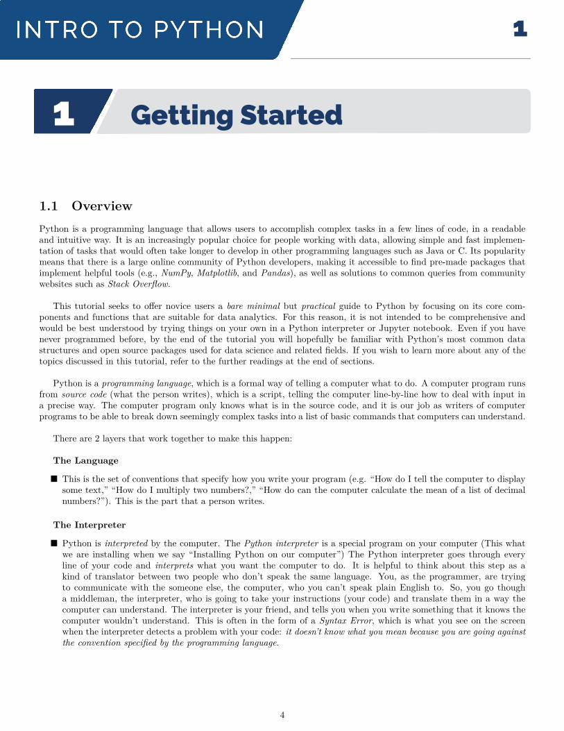
1.1 OverviewPython is a programming language that allows users to accomplish complex tasks in a few lines of code, in a readableand intuitive way. It is an increasingly popular choice for people working with data, allowing simple and fast implemen-tation of tasks that would often take longer to develop in other programming languages such as Java or C. Its popularitymeans that there is a large online community of Python developers, making it accessible to find pre-made packages thatimplement helpful tools (e.g., NumPy, Matplotlib, and Pandas), as well as solutions to common queries from communitywebsites such as Stack Overflow.

This tutorial seeks to offer novice users a bare minimal but practical guide to Python by focusing on its core com-ponents and functions that are suitable for data analytics. For this reason, it is not intended to be comprehensive andwould be best understood by trying things on your own in a Python interpreter or Jupyter notebook. Even if you havenever programmed before, by the end of the tutorial you will hopefully be familiar with Python’s most common datastructures and open source packages used for data science and related fields. If you wish to learn more about any of thetopics discussed in this tutorial, refer to the further readings at the end of sections.

Python is a programming language, which is a formal way of telling a computer what to do. A computer program runsfrom source code (what the person writes), which is a script, telling the computer line-by-line how to deal with input ina precise way. The computer program only knows what is in the source code, and it is our job as writers of computerprograms to be able to break down seemingly complex tasks into a list of basic commands that computers can understand.

There are 2 layers that work together to make this happen:

The Language

■ This is the set of conventions that specify how you write your program (e.g. “How do I tell the computer to displaysome text,” “How do I multiply two numbers?,” “How do can the computer calculate the mean of a list of decimalnumbers?”). This is the part that a person writes.

The Interpreter

■ Python is interpreted by the computer. The Python interpreter is a special program on your computer (This whatwe are installing when we say “Installing Python on our computer”) The Python interpreter goes through everyline of your code and interprets what you want the computer to do. It is helpful to think about this step as akind of translator between two people who don’t speak the same language. You, as the programmer, are tryingto communicate with the someone else, the computer, who you can’t speak plain English to. So, you go thougha middleman, the interpreter, who is going to take your instructions (your code) and translate them in a way thecomputer can understand. The interpreter is your friend, and tells you when you write something that it knows thecomputer wouldn’t understand. This is often in the form of a Syntax Error, which is what you see on the screenwhen the interpreter detects a problem with your code: it doesn’t know what you mean because you are going againstthe convention specified by the programming language.

4

1.2 InstallationJupyter notebooks are a popular way of interfacing with Python. You write code and execute it through the browser ina visual way rather than from a command line.

The simplest way to install Python on your computer for the purposes of the exercises in this book is to use Anaconda,which is a version of Python that includes all of the scientific computing tools you need. It also comes with both Jupyternotebook and the command line version of python, so you can choose which interface you need. Download the packagefrom the official Anaconda distribution website and then follow the instructions that correspond to the operating systemon your computer (e.g., if you have a Windows computer, choose the Windows downloader instead of Mac).

1.3 Running PythonThere are multiple ways of running python. If you’re just getting started, or if you’re using this tutorial book alongside acourse that uses Jupyter, it is best to run it from a Jupyter notebook.

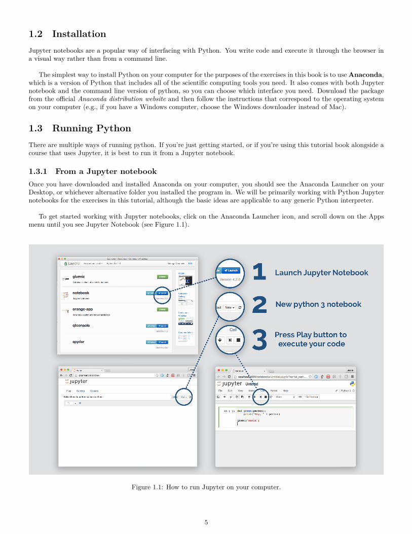
1.3.1 From a Jupyter notebookOnce you have downloaded and installed Anaconda on your computer, you should see the Anaconda Launcher on yourDesktop, or whichever alternative folder you installed the program in. We will be primarily working with Python Jupyternotebooks for the exercises in this tutorial, although the basic ideas are applicable to any generic Python interpreter.

To get started working with Jupyter notebooks, click on the Anaconda Launcher icon, and scroll down on the Appsmenu until you see Jupyter Notebook (see Figure 1.1).

Figure 1.1: How to run Jupyter on your computer.

5

1.3.2 From the command lineIf you do not want to use the graphical interface of the Jupyter Notebook to execute python, or wish to use your ownfavorite text editor (such as Sublime Text or Vim) to write your python files, you can also run python from the commandline.

Figure 1.2: How to run python from the command line.

1.4 An exampleThis section provides a simple example to get you started by printing the content of a variable in python. A variablestores something in memory so you can refer to it over and over again using the name you assign to it. Let’s right awaylook at an example of a variable used in a full Python program.

1 #My f i r s t program . This d isp lays a simple message on the screen .2

3 my_message = ”Greetings , Earth ! ”4

5 print (my_message)

Line-by-line breakdownLine 1: The number (or hashtag) symbol # is how you define a comment in Python. When you start a line in

your code with a number symbol, it lets Python know that it should ignore everything after that symbol. You can writeanything here, and should always leave descriptive comments in your code explaining what you’re doing, otherwise it willbe very difficult for another person to understand your code.

Line 3: Here is where you assign the variable. The syntax for assignment is the equals sign. A variable can be calledanything, under these restrictions:

• A variable name must start with a lowercase or uppercase letter, no numbers or underscores.

6

• A variable may contain any amount of underscores or numbers anywhere in the variable name except the beginning,but no other non-alphabetic symbols. ( like $ , & , * , etc... )

Line 5: We pass the variable name we created into the print() function. Later we will be defining our own functions, butfor now, all we need to know is that you can pass variables into functions, referred to as function arguments in this case.

That’s it! This is your first Python program. We will soon be getting to more complex tasks beyond displaying texton a screen, but this exercise is helpful in making sure we understand the basic terminology and ways to call functionswhich we will use later in this series.

The rest of this document is organized into two main section. Section 2 describes the core set of data structures inPython, and how you might operate and visualize them. Section 3 describes common tools in Python, including state-ments, built-in and external functions that you will come across in Section 2. A recommended way of learning this tutorialis to go through the examples in Section 2 in Python and cross-reference with materials in Section 3.

Enjoy!

7

Chapter 2

Data StructuresData Structures2

2

A data structure is a specialized way of storing information in a program. There is no single best data structure thatworks for every situation. Data structures have different properties that are optimized to fit a specific kind of application,and a structure that works perfectly fine for one situation may be terrible for another. In practice, engineers and datascientists care about runtime, which is the way in which the computation time grows with the size of input. In this tutorialhowever, we won’t be encountering data so large that a less-than-optimal choice in data structure will prevent us fromcompleting the task. Nonetheless, it is crucial to understand the differences between data structures to know which is themost efficient (and often most convenient) choice to implement.

2.1 ListA list in python is exactly what it sounds like: a collection of objects in a particular order, separated by commas. Forexample:

1 animals = [ ’dog ’ , ’ rabbit ’ , ’ duck ’ , ’ goat ’ , ’ bear ’ ]

This creates a list of strings (eg ’dog’) that will stay in the exact same order unless you change it. If you need to accessthe list, you can call a function such as:

1 print ( animals )

and will get back your unchanged list:1 [ ’ dog ’ , ’ rabbit ’ , ’ duck ’ , ’ goat ’ , ’ bear ’ ]

For strings, you can use either single quotes or double quotes; i.e ”dog” and ’dog’ are equivalent. However, ’dog” willgive you an error, because you must start and begin the string declaration with the same kind of quote character.

You can put any kind of object in a list.1 d i g i t s = [3 ,1 ,4 ,1 ,5 ,9 ,2 ,6 ,5 ,3 ,5 ]

is a list of integers. Notice that integers don’t have quotes around them. If you were to put quotes, they would becomestrings, not integers.

You can also put objects of mixed types in a list. For example, try putting the string ’high’ and the integer 5 in thesame list.

2.1.1 Basic operations2.1.1.1 Accessing an element in a list

If you know the index of the element in your list, you can use the following bracket notation to get that element.1 f r u i t s = [ ’banana ’ , ’ orange ’ , ’watermelon ’ , ’ grape ’ , ’ strawberry ’ ]2

3 f i rst_element = f r u i t s [ 0 ]

The number inside the brackets is the index of the item. Remember, python is zero-indexed, which means elements in asequence will start counting at 0 instead of 1. Given this convention, how would you index the last element, “strawberry,”in the above list?

8

2.1.1.2 Accessing parts of a list

If you need to get the elements of a list between certain indices, you can use a variant of the bracket notation usedpreviously.

1 all_numbers = [0 ,1 ,2 ,3 ,4 ,5 ,6 ,7 ,8 ,9 ]2

3 f i r s t_three = all_numbers [ 0 : 3 ]4 print ( f i r s t_three )

This gets the first three numbers in the all_numbers list and puts them in a variable called “first_three.”

2.1.1.3 Iterating over a list

Sometimes you need to go through all the elements in a list in order. For that, you use a for loop, which uses a variableto point to each element in the sequence, starting at the first one.

1 co lo r s = [ ’ red ’ , ’ orange ’ , ’ yellow ’ , ’ green ’ , ’ blue ’ , ’ indigo ’ , ’ v i o l e t ’ ]2

3 f o r co lor in co lo r s :4 print ( co lor )

It doesn’t matter what you call the variable you use to point to the elements. Instead of calling it “color,” we couldhave as well called it “Jeffrey,” and it would have still performed the same task. However, it is good practice to useinformative names for your variables. Note that in order to step through the objects in the list, we have used the for loopwhich allows iteration over a defined sequence - see Section 3.1.2 for more details.

2.1.1.4 Obtaining a random element from a list

1 import random2

3 some_numbers = [1 ,2 ,3 ,4 ,5 ,6 ,7 ]4 n = random . choice (some_numbers)5 print (n)

This uses a function in the built-in package called “random.” There are other useful tools in the random package,which are listed in the online documentation at python.org .

2.1.1.5 Randomizing a list

1 import random2

3 some_numbers = [1 ,2 ,3 ,4 ,5 ,6 ,7 ]4 random . shu f f l e (some_numbers)5 print (some_numbers)

2.1.1.6 Reversing indices

If you specify a negative number as your index, it the python interpreter will count backwards starting from the end ofthe list.

This is useful when you don’t exactly know the length of the list you are operating on, but know that you want elementsup to a fixed number from the end of the list. (e.g. all elements except for the last)

1 food = [ ”apple” , ”beet” , ” carrot ” , ”dinner” ]2

3 #thi s s l i c e operation takes a l l elements from the beginng4 #ending before the l a s t value of the l i s t5 food_section = food [0:−1]6

7 print ( food_section )

9

2.1.1.7 List comprehension

List comprehension provides a compact way of constructing a new list based on an existing list. For example, youcan create a list with new values on the fly by iterating through an existing sequence using the special condensed listcomprehension syntax. This makes code easier for you to write, but beware, list comprehensions may make it harder forsomeone else to read your code.

First let’s take a look at a regular python for loop, applied to square the numbers from an input list, and create a newlist with those values.

1 even_numbers = [2 ,4 ,6 ,8 ,10 ]2

3 #create a new l i s t to store the re su l t ing values .4 even_squares = [ ]5

6 f o r num in even_numbers :7 even_squares . append(num**2)

We can iterate through all the values using the for loop syntax, detailed above. However, we can bypass this syntaxby using a list comprehension.

1 even_numbers = [2 ,4 ,6 ,8 ,10 ]2

3 #square the numbers and put them in a new l i s t4 even_squares = [n**2 for n in even_numbers ]

1 Lowercase_book_title = [ ” a l i c e ” , ” in ” , ”wonderland” ]2

3 cap i ta l i z ed_t i t l e = [word . c ap i t a l i z e () fo r word in Lowercase_book_title ]

A hard to read list comprehension Be careful with putting too many nested operations in a single list compre-hension.

1 even_numbers = ”2 4 6 8 10”2

3 gobbldeygook = [ ”number : ” + st r (( int ( e ) **2 + int (4 * int ( e )*5+2)) ) fo r e in reversed (even_numbers . s p l i t ( ) ) ]

2.1.1.8 Reversing a list

1 all_numbers = [0 ,1 ,2 ,3 ,4 ,5 ,6 ,7 ,8 ,9 ]2

3 reversed_l i s t = [ num for num in reversed ( all_numbers ) ]4 print ( reversed_l i s t )

This one-line solution to reversing a list makes use of the built-in reversed() function and list comprehension.

2.1.2 VisualizationLists are used as input for some of the most common graphs. For example, a scatter plot is just a visualization of twolists: a list of x values and a list of y values. The same goes for most pie charts, bar graphs, and histograms.

2.1.2.1 Pie chart

The most common graphing package is matplotlib. For convenience, all of its functions come built in to pylab, which isalready installed on your jupyter accounts. Once you import all of the functions in the package, you can use the pie()function. Note: If you are using a generic Jupyter notebook, you will need to insert the line “%matplotlib inline” at thetop of your program for any graphics to work properly.

1 from pylab import *2

3 #This i s the data we w i l l be p lott ing4 counts = [6 , 3 , 2 , 2 , 2 , 1 , 1 ]5 categor i e s = [ ’ Cognitive Science ’ , ’Computer Science ’ , ’Data Science ’ , ’ Stats ’ , ’ L ingu i s t i c s ’ , ’Machine

Learning ’ , ’Cool Class ’ ]6

7 #Set up a pie chart with the data using the pie () function8 pie ( counts , l abe l s=categor ies , autopct=’%1.1 f%%’ )

10

9

10 #Add an informative t i t l e11 t i t l e ( ’Reasons For Taking This Course ’ )12

13 #Display the pie chart14 show()

2.1.2.2 Scatter plot

A scatter plot is useful for visualizing lists of numbers, as it can help you notice trends graphically.1 from matplotl ib . pyplot import *2

3 #This i s the data we w i l l be p lott ing4 x = [1 ,2 ,3 , 4 , 5 ]5 y = [2 ,4 ,6 ,8 ,10 ]6

7 #Plot the data8 scat te r (x , y)9

10 t i t l e ( ”X vs Y”)11

12 show()

2.1.2.3 Bar plot

A bar plot is useful when you have a large amount of long labels for data that are all important to see, when a differentgraphing technique might bunch the labels together.

1 import matplotl ib . pyplot as p l t2

3 major_labels = [ ’Computer Science ’ , ’ Cognitive Science ’ , ’ S t a t i s t i c s ’ , ’EECS’ , ’Comparat ive Literature ’ , ’Undecided ’ , ’Economics ’ , ’ Legal Studies ’ , ’Math ’ , ’ Business ’ , ’IEOR’ , ’Po l i t i c a l Economy ’ , ’ Sociology ’ , ’Psychology ’ ]

4 major_counts = [10 ,7 ,1 ,2 ,1 ,3 ,3 ,1 ,2 ,2 ,1 ,1 ,1 ,1 ]5

6 #Graph Breakdown of Majors In The Course7 y_pos = np . arange ( len (major_labels ) )8

9 plt . barh (y_pos , major_counts , a l ign=’ center ’ , alpha=0.4)10 plt . yt icks (y_pos , major_labels )11 plt . x labe l ( ’Amount of Students In Major ’ )12 plt . t i t l e ( ’Breakdown of Majors in Class ’ )13

14 plt . show()

2.1.3 Further readingsFor a more comprehensive reference on lists in python: https://docs.python.org/2/tutorial/datastructures.html

2.2 ArraySimilar to a list, a numpy array is an ordered collection of objects. The biggest difference between how you use a numpyarray and python’s built-in list object is that once you create a numpy array, you cannot change the amount of elementsit contains.

This constraint allows for things under the hood of python to be more efficient, so operations like “sum” and “product”will take less time to calculate. This becomes more apparent when working with large amounts of data.

Numpy is an example of an external package, which is a set of tools written by a third-party that you can use in yourprograms by including an import statement at the top of your program. An array is only one of the many data structuresand functions that come included in the numpy package. See Section 3 for details on

Take this for example:

11

1 import numpy2

3 deposit_history = numpy. array ( [ 3 , −2, 8 , 2 , −2, 29] )4

5 account_balance = deposit_history . sum()6

7 print ( ”Total balance i s : ” )8 print ( account_balance )

Line-by-line breakdown

Line 1: This is the import statement which tells the python interpreter that you want to use tools from the numpypackage.

Line 3: This creates a new numpy array containing the values in the given list, and assigns that array to the variablename deposit_history.

Line 5: This creates a new variable called account_balance, which is assigned the value resulting from summing upall the numbers in deposit_history. The function .sum() is a function that comes with numpy arrays. If you try to call.sum() on a regular python list, this will cause an error.

You should use numpy arrays instead of regular python lists for as many computations as you can, due to the array’sfaster speed and built-in functions.

2.2.1 Basic operationsIf you would like to scale your array by a constant factor, you can multiply it using the python multiplication syntax.

1 import numpy2

3 grade_history = numpy. array ( [ .48 , .42 , .45 , .48 , .39 ] )4

5 better_grades = 2 * grade_history6

7 print ( better_grades )

You can use the same python syntax for all basic operations that you would normally do on numbers.

1 grades_plus_one = grade_history + .012

3 grades_squared = grade_history ** 24

5 lower_grades = grade_history − .256

7 halved_grades = grade_history / 2.0

Notice the division operation on halved_grades. We divided by 2.0 because if we had divided by the integer 2 withoutthe decimal, then python would have rounded down automatically for uneven divisions. Try it for yourself and see thedifference.

2.2.1.1 Taking the logarithm

Numpy has a logarithm function, which you can pass arrays into.1 tree_trunk_heights = numpy. array ( [25 , 26 , 77 , 108 , 15 , 98 ] )2

3 log_of_trunks = numpy. log ( tree_trunk_heights )

Notice we didn’t do tree_trunk_heights.log() This is because the function logarithm is not built into the actual numpyarray itself. It is an external function that is included in numpy, so you use it by passing the array into it rather thancalling it from the array object. This is the case for many of the more complex numpy functions, which you can readabout in the numpy documentation.

12

2.2.1.2 Taking the absolute value

You can take the absolute value of the elements of an array using a numpy function.1 import numpy2

3 distances_travel led = numpy. array ( [−11 , 20 , 99 , 11 , −2, 10 , −23] )4

5 absolute_distances = numpy. absolute ( distances_travel led )

2.2.1.3 Taking the mean of a single array

Sometimes you need to know what the average of an array of numbers is. There is a convenient built-in mean function innumpy arrays that you can use.

1 import numpy2

3 grade_history = numpy. array ( [ .98 , .82 , .65 , .88 , .91 ] )4

5 score_in_class = grade_history .mean()6

7 print ( ”Your grade i s : ” )8 print ( score_in_class )

2.2.1.4 Taking the mean of multiple arrays

Taking the mean between multiple arrays is slightly different. This is because instead of a single number that representsthe average value for a single array, we want a whole array that represents the pairwise average between values of multiplearrays. Instead of using the array’s built in mean() function which returns a single value, we will use numpy’s mean()function. This is how the syntax differs:

1 import numpy as np2 ”””3 we import numpy as np because i t gets tedious to retype ”numpy” every time we need to4 c a l l a function . We could have ca l l ed i t anything we want ( eg import numpy as blablabla )5 but i t i s convention to c a l l i t np as an abbreviation .6 ”””7 my_grade_history = np . array ( [ .98 , .82 , .65 , .88 , .91 ] )8

9 friend_grade_history = np . array ( [ . 8 8 , .98 , .60 , .90 , .72 ] )10

11 ”””12 The arrays must be passed in together in a tuple rather than separate ly13 Also , we say axis=0 because we want the average to be computed column wise , that i s , f o r every element14 rather than row wise ( axis=1) , which would give a s ing l e r e su l t fo r each array15 ”””16 averages_between_us = np .mean( ( my_grade_history , friend_grade_history ) , axis=0 )17

18

19 print ( ”Our combined average on each assignment i s : ” )20 print ( averages_between_us )21

22 student_1 = np . array ( [ .98 , .82 , .65 , .88 , .91 ] )23 student_2 = np . array ( [ .72 , .58 , .80 , .97 , .79 ] )24 student_3 = np . array ( [ .89 , .78 , .65 , .93 , .78 ] )25 student_4 = np . array ( [ .90 , .95 , .70 , 1 .00 , .89 ] )26 student_5 = np . array ( [ .83 , .91 , .69 , .98 , .90 ] )27 student_6 = np . array ( [ .87 , .42 , .81 , .90 , .77 ] )28 student_7 = np . array ( [ .80 , .92 , .72 , .70 , .76 ] )29

30 class_averages = np .mean( ( student_1 , student_2 , student_3 , student_4 , student_5 , student_6 , student_7 ) , axis=0 )

31

32 print ( ”The average fo r each assignment in the c l a s s i s : ” )33 print ( class_averages )

13

2.2.1.5 Operating over multiple arrays

The same way we can use the built in python syntax to do numeric operations over a single array, we can do thoseoperations between multiple arrays .

1 import numpy as np2

3 a = np . array ( [1 , 2 , 3 , 4 ] )4 b = np . array ( [10 , 20 , 30 , 40] )5

6 #multiply the arrays7 print ( b * a )8

9 #divide the arrays10 print ( b / a )11

12 #add the arrays13 print ( b + a )14

15 #subtract the arrays16 print ( b − a )17

18 #exponentiate the arrays19 print (b ** a )

2.2.1.6 Converting arrays to lists

1 import numpy as np2

3 words_per_book = np . array ( [21222 , 8119 , 1999 , 3726 , 1217 , 1192 , 12187 , ] )4

5 words_per_book_list = words_per_book . t o l i s t ( )

2.2.1.7 Converting lists to arrays

1 import numpy as np2

3 words_per_book_list = [21222 , 8119 , 1999 , 3726 , 1217 , 1192 , 12187 , ]4

5 words_per_book_array = np . array (words_per_book_list )

2.2.2 VisualizationArrays can be used as the input to many plotting functions, the same way lists can be. The following sections will showdifferent application of visualization using numpy arrays.

2.2.2.1 Histogram

You can graph a histogram using numpy arrays as well as python lists.1 import matplotl ib . pyplot as p l t2 import numpy as np3

4

5 vegetable_labels = [ ’Radish ’ , ’ Spinach ’ , ’ Carrot ’ , ’ Eggplant ’ , ’Peas ’ , ’ Broccol i ’ , ’ Caul i f lower ’ , ’ Beet ’ ]6 vegetable_counts = np . array ( [1 , 20 , 4 , 21 , 16 , 1 , 10 , 15] )7

8 #Graph breakdown of Favorite Vegetables9 y_pos = np . arange ( len ( vegetable_labels ) )

10

11 plt . barh (y_pos , vegetable_counts , a l ign=’ center ’ , alpha=0.4)12 plt . yt icks (y_pos , vegetable_labels )13 plt . x labe l ( ’Votes fo r Vegetable ’ )14 plt . t i t l e ( ’ Favorite Vegetable Survey ’ )15

16 plt . show()

14

2.2.2.2 Scatter plot

A scatter plot is especially useful when you want to show the relationship between two numeric variables, which correspondto the x and y axes.

1 import matplotl ib . pyplot as p l t2 import numpy as np3

4 ”””5 Each of these var iab le dec larat ions should be on one l ine , but may appear6 cut o f f on d i f f e r en t text ed i to r s . I f you come across th i s in other tu t o r i a l s or in c lass ,7 know that when you input the data yourse l f , to do so in a s ing l e l i n e .8 ”””9 hours_studied = np . array ( [0 ,1 ,2 ,3 ,4 ,0 ,0 ,2 ,0 ,3 ,4 ,5 ,2 ,10 ,2 ,1 ,2 ,0 ,1 ,2 ,3 ,4 ,3 ,1 ,3 ,5 ,1 ,7 ,8 ,10 ,9 ,10 ,1 ,2 ,3 ,0 ] )

10 grade_on_exam = np . array ( [ 0 , . 1 0 , . 1 0 , . 3 , . 4 0 , . 1 0 , . 2 0 , . 2 2 , 0 , . 3 3 , . 5 4 , . 4 5 , . 2 6 , 1 . 0 , . 2 , . 1 , . 2 5 , . 2 0 , . 1 ,11 . 2 3 , . 2 3 , . 4 4 , . 2 3 , . 1 5 , . 3 0 , . 5 5 , . 1 1 , . 7 0 , . 8 9 , 1 . 0 0 , . 9 2 , . 9 3 , . 1 3 , . 2 5 , . 3 1 , . 3 3 ] )12

13 plt . s cat te r ( hours_studied , grade_on_exam)14 plt . x labe l ( ’Hours Studied ’ )15 plt . y labe l ( ’Grade On Exam’ )16 plt . t i t l e ( ’Hours Studied vs Grade On Exam’ )17

18 plt . show()

2.2.2.3 Log-log Plot

A log-log plot visualizes the logarithm of the data instead of the raw numerical data. This helps uncover certain nonlinearrelationships visually.

1 import matplotl ib . pyplot as p l t2 import numpy as np3

4 # Generate some data .5 x = np . l inspace (0 , 2 , 1000)6 y = x**np . e7

8 #This graph w i l l show a nonlinear re la t i onsh ip between the data , which may be hard to inte rpre t v i sua l l y .9 plt . s cat te r (x , y)

10 plt . show()11

12 #This graph w i l l c l e a r l y show a l in ea r re la t i onsh ip between the log of the data .13 plt . log log (x , y)14 plt . show()

2.2.3 Further readingsThe numpy documentation describes more numerical operations and functions on arrays:http://docs.scipy.org/doc/numpy/reference/arrays.ndarray.html

Matplotlib is the library which lets you graph with python. This gallery shows many example plots:http://matplotlib.org/gallery.html

2.3 DictionaryDictionaries (sometimes referred to as hash tables or hash maps) are one of the most powerful data structures in computing.They operate on the fastest possible runtime for insertion and access of values: constant time. For this reason, dictionarieshave profound applications in data science and software engineering. This tutorial will discuss the foundations of howdictionaries are able to accomplish this speed, as well as some of the principles of indexing, and what this means for listsand the other structures we have discussed thus far.

15

2.3.1 Basic operations2.3.1.1 Indexing

Indexing refers to the process of accessing the values of a data structure using an index, which is usually an integerrepresenting a specific location in that structure.

Take this for example:

Figure 2.1: ”animal_weights”, a regular python list

1 animal_weights = [ ( ’dog ’ , 65) , ( ’mouse ’ , 0.042) , ( ’ bird ’ , 0 .66) , ( ’ cat ’ , 8 .2) ]2

3 cat_element = animal_weights [ 3 ]4 print ( cat_element [ 1 ] )

This code creates animal_weights which is a list of tuples, where the first tuple element is the animal’s name and thesecond element of the tuple is the animal’s average weight.

We then access the “cat” element, which by looking at code, we know is at index 3 in the list, and print out its averageweight.

This is the best-case scenario, in which we already know the index where the value we care about it stored. Since wecan just go directly to that index, this takes only 1 computation step to get the information we need.

What if we didn’t know what index the cat element was at?We would have to perform a linear search using a for loop,where we start at the beginning of the list, iterating through every element to check if it is the one where the ”cat” weightis stored:

1 f o r element in animal_weights :2 i f element [ 0 ] == ’ cat ’ :3 print ( element [ 1 ] )

You can see from this for loop, that this is not the most efficient way to store value pairs like this. When the elementwe care about is towards the very end of the list, we have to iterate through all the elements before we get to it. In thisworst case scenario, it takes n computation steps, where n is the length of the list we are searching through.

How can we ensure that we always know the index of every element, regardless of sorting and order added?

2.3.1.2 Hashing

Dictionaries are a kind of data structure that achieve retrieval of value when given a corresponding key in 1 computationstep. This is possible through a mathematical trick called hashing, which we will discuss briefly a high level.

2.3.1.3 Key-value pairing

Dictionaries rely on an internal hash function, which is a mathematical function that, in principle, assigns a unique integerto any key. A key can be almost any python object, though strings are the most common key to use, because they areintuitive to think about in a key - value pairing.

Because we don’t have to ever look up the index for any key, since it is computed on the fly, we can no have the indexto any key in one computational step. It is important to note, the hash function doesn’t just assign a random number;it computes a unique integer that will always be the same for any given key. This is how we are able to guarantee that wecan retrieve the value corresponding to this key. The specifics for exactly how hash functions work are out of the scope ofthis tutorial. We will now continue by showcasing how to use a dictionary, python’s hash-powered data structure.

16

Figure 2.2: How a dictionary works under the hood.

2.3.1.4 Using a dictionary

1 #syntax for de f in ing a new dict ionary2 animal_weights = {}3

4 #adding key−value pa i r s to the dict ionary5 animal_weights [ ”dog” ] = 656 animal_weights [ ”mouse” ] = 0.0427 animal_weights [ ”bird ” ] = 0.668 animal_weights [ ” cat ” ] = 8.29

10 #ret r i ev ing a value given a key11 cat_weight = animal_weights [ ” cat ” ]12

13 print ( cat_weight )

2.3.1.5 Sorting values in a dictionary

Sometimes you want to see the order a dictionary’s values take on after populating the dictionary. Since you can onlyaccess a value by passing in its corresponding key, you have to iterate over the list using a built-in package.

1 import operator2

3 #we sort the dict ionary based on the keys using itemgetter4 sorted_weights = sorted ( animal_weights . items () , key=operator . itemgetter (1) )5

6 #sorted_weights w i l l be a l i s t of tuples sorted by the weight7 print ( sorted_weights )8

9 #I f we want the biggest weights f i r s t , we can reverse the l i s t10 descending_weights = [w for w in reversed ( sorted_weights ) ]11

12 print ( descending_weights )

2.3.2 Further readingsFurther readings on dictionaries can be found at https://docs.python.org/3/tutorial/datastructures.html.

2.4 PandasWhat is pandas? Pandas is a library for data analysis. It provides helpful classes and functions which you can use inyour programs to do work with real world data. It is different from numpy in that it centers on the idea of a Data Frame,which is a data structure that makes it easier to work with labeled row-column formatted data (like a csv file).

To illustrate functions in Pandas, e will be working with real data taken from http://ucpay.globl.org/ . In this mini-example, we have downloaded data and put it in a csv called 2014TopPay.csv . It contains data from four UC campusesdetailing the single top earning employee in each of four department categories in 2014 in the following table.

A pandas data frame is one of the most popular ways to work with csv data in python. To read this csv into yourprogram, first make sure it is in the same directory as your .py file or ipython notebook. Then you can access it using theread_csv function:

17

Table 2.1: 2014TopPay.csvCAMPUS COMPUTER_SCIENCE BUSINESS/ECONOMICS ATHLETICS LAW

BERKELEY 215,410 812,489 1,805,400 546,057LOS_ANGELES 160,282 599,535 3,476,127 458,918

DAVIS 203,519 452,611 237,987 458,918IRVINE 323,692 470,066 334,008 346,398

1 from pandas import read_csv2

3 s a l a r i e s = read_csv ( ’ 2014TopPay . csv ’ )

’salaries’ is now a pandas Data Frame, which you can get a preview of by passing it into the print() function.

2.4.1 Basic operations2.4.1.1 Averaging

Pandas Data Frames come with a built-in function .mean() which you can call directly from the object itself. Since thisexample is a 2 dimensional data structure, there are two different means we could be interested in: column-wise androw-wise.

Column-wise meanTaking the column-wise mean will give us the average top-pay by department.

1 average_by_department = sa l a r i e s .mean( axis=0)2

3 print (average_by_department )

The ’axis’ argument tells the mean function whether you want column-wise or row-wise mean.

Row-wise meanTo take the row-wise mean, we can just change axis to equal 1 instead of 0. In this example, the row wise mean tells

us each university’s average salary for the top earners in the departments we have listed.1 average_by_university = sa l a r i e s .mean( axis=1)2

3 print ( average_by_university )

Notice though, the mean() operation can be crude and misleading, especially in the presence of outliers. For example,if we just looked at the results from the above calculation, we would only see that the mean top-earning value at UCLAwas about 1.5 million, and not see that it was being skewed by a single extreme value while most values were more spreadout on a larger spectrum.

2.4.1.2 Standard deviation

The standard deviation provides us more information beyond what is summarized by the mean alone. It is a measure ofhow spread-out a data set is, and it does so by providing a metric for how far data points are from the average of thatdata. A standard deviation close to 0 means that the data is closely packed together, while a larger standard deviationmeans it is spread out over a bigger range of values.

Similar to the case of averaging, we can take the standard deviation both column-wise and row-wise using the .std()function built-in to pandas data frames.

Column-wise standard deviation1 std_per_department = sa l a r i e s . std (0)2 print ( std_per_department )

Row-wise standard deviation1 std_per_university = sa l a r i e s . std (1)2 print ( std_per_university )

18

Now that we know the row-wise standard deviation is large, we know to be more skeptical about considering UCLA’srow-wise mean as very representative of the whole data set.

2.4.1.3 Conversion to arrays

To convert any part of a Pandas Data Frame to a numpy array, you can use the .as_matrix() function built-in to theData Frame object.

1 athlet ic_array = sa l a r i e s [ ’ATHLETIC’ ] . as_matrix ()

Now you can apply any numpy array function on this new object.

2.4.2 Further readingsDocumentation on pandas can be found at http://pandas.pydata.org/.

19

Chapter 3

Tools Tools3

3

This chapter is a reference of many tools that are central to a data scientist using python on a regular basis. You willfind that even as you learn other programming languages that may call these tools by different names, the core functionsof how they work will carry over, and having a strong grasp on these now will help in countless applications to come.

3.1 StatementsStatements are special keywords in Python that perform various functions such as directing the flow of the program inresponse to different inputs and data. This allows for it to branch out into different cases and to execute some parts ofthe code conditionally. Using these keywords makes your code more general and powerful, dealing with different kinds ofinputs in different ways rather than just being a single sequential script.

3.1.1 import statementThe import statement provides additional functionality to your code, allowing you to use external packages, which arecollections of classes and functions that you don’t have to write yourself. Examples of packages are:

• random - Includes functions that deal with generating random numbers.

• time - Helpful tools for timing your program.

• os - Interact with parts of the computer that wouldn’t otherwise be accessible to a python script, such as shellcommands.

3.1.2 for loopA for statement is most commonly associated with the for loop. You can use for to iterate over a sequence of any iterable

type. A good rule of thumb for telling whether a type is iterable is: If it is a collection of potentially more than oneelement, then it is likely iterable.

Take this example:1 five_numbers = [1 ,2 ,3 , 4 , 5 ]2

3 f o r number in five_numbers :4 print (number)

The list contains a sequence of values over which we can iterate. What the for statement does is assign the variablenumber to each element of the list, one by one as it iterates through the values. On the first iteration, number will beset to the value 1, and we will therefore pass the number 1 to the print function, which will display that value. On thesecond iteration, it will equal 2, and so on.

3.1.3 if statementThe conditional statement if is what allows your program to branch out into different cases given some values of input.The structure for how to use these statements is as follows:

if CONDITIONAL STATEMENT:(TAB) Execute some codeThe TAB (or alternatively 4 spaces) lets python know that everything that is indented is part of the inside of the if

statement. A Conditional Statement is anything that can evaluate to True or False.

20

1 i f True :2 print ( ”Yes , i t ’ s true ! ” )

In this above example we use the python statement True, which indeed always evaluates to True. The if statement ismost useful when dealing with statements that might be True in some cases and False in others.

How do you direct your code if the Conditional Statement is False? Use an else statement. This lets your code branchout to a different chunk. For example:

1 def check (number) :2 i f number%2 == 0:3 print ( ”Number i s Even ! ” )4 e l s e :5 print ( ”Number i s Odd! ” )6

7 check (5)

The above code checks the properties of a number given to the function, and executes a different chunk of code incases where the Conditional Statement (number%2 ==0) is True or False.

3.1.4 while statementThe While statement allows for repeated execution of a particular section of code, as long as certain properties are met.It starts at the top with the conditional statement, and follows this structure:

While CONDITIONAL STATEMENT:(TAB) Execute some code.The conditional statement must always evaluate to either a True or False value. If the conditional statement returns

anything else, the program will error. The most important aspect of writing a while loop is to ensure that it will terminate.If you aren’t properly updating the variable your conditional statement is checking, the statement might always be True,and it will loop forever!

The example code below demonstrates a use of a while loop in combination with a function that returns either a Trueor False value.

1 def is_ok (number) :2 #This function checks certa in propert i e s of a number3 # I f a l l propert i e s are met , i t returns True , otherwise returns False4 i f number !> 5:5 return False6 i f number%7 == 1:7 return False8 i f number > 10000:9 return False

10 return True11

12 number = 613 while is_ok (number) :14 print ( ”The number i s s t i l l ok . ” )15 number = (number * 3) − number/216

17 print ( ”The number i s no longer ok . ” )

The above code uses a function that returns a True or False value. Refer to the Section 3.2 for more information aboutwhat functions.

3.2 FunctionsThis tutorial will use terms dealing with functions.

3.2.1 Creating a functionIn computer science, functions are processes that take in any amount of values and do something with those values. Hereis the syntax for defining a simple function:

1 def greet (name, age ) :2 print ( ”Hello , my name i s ” + name)3 print ( ” I am ” + age + ” years old” )

21

Let’s take a look at the details of what this piece of code means. The ’def’ keyword tells python that you are aboutto define a new function, whose name follows immediately after this keyword. Accordingly, ’greet’ is the name we gaveto it. Function names can contain letters, numbers, and underscores only, but cannot start with a number. If you wantto give your function a name with multiple words, it is convention to separate the words with underscores, as in ”defgreet_my_friends():”. For more style conventions, see the PEP style guide, provided in Further Readings.

After the function name, you write the names of all the arguments your function requires, separated by commas. Thesemust be enclosed in parentheses, with a colon ”:” following immediately after. This tells the python environment thatwhat follows is the body of the function, which is where you write everything the function does, and must be indented by4 spaces. Finally, a function can have a return value, which is the output that the function gives. For example:

1 def square (x) :2 return x * x

In this way, your function can pass a value to other functions. Once you use the ’return’ keyword, your function halts,and returns what results from evaluating the statement that immediately follows. Now you can call your functions bypassing in all of the required arguments with parentheses:

1 greet ( ”Luz” , 19)2

3 #This i s to show that you can do operations on values returned from funct ions you def ine .4 square_plus_two = 2 + square (5)5

6 print ( square_plus_two)

3.2.2 Built-in functionsPython includes many built-in functions without you having to import them from an external package. This section willprovide a brief reference for them.

3.2.2.1 random.choice()

Picks a random choice from a collection of objects, such as a list.1 import random2

3 numbers = [1 ,2 ,3 , 4 , 5 ]4

5 random_number = random . choice (numbers)

3.2.2.2 random.shuffle

Randomizes a list or other ordered sequence object in-place. This means it does not return an object, but rather changesthe original object itself.

1 import random2

3 sorted_numbers = [1 ,2 ,3 , 4 , 5 ]4

5 random . shu f f l e ( sorted_numbers )

3.2.2.3 reversed()

Creates an iterator that contains the reversed version of the iterable passed in. The iterable can be any object with anorder, such as a list or array. Notice, it creates an iterator, not a duplicate object, which means you need to iterate overit to get through all the objects using a for loop or list comprehension.

1 in_order = [1 ,2 , 3 , 4 ]2

3 #thi s i s not a l i s t , i t ’ s an i t e r a to r4 reversed_order = reversed ( in_order )5

6 #extract the objects from the i t e r a to r to get them into a l i s t7 reversed_l i s t = [ object fo r object in reversed_order ]

22

3.2.2.4 print()

The print function takes in an object that can be converted into a string and displays it as output.

For example:1 #displays the s t r ing2 print ( ”Hello there ” )3

4 #displays the integer5 print (25)

Notice that print takes in any type of object, not just a string.

3.2.2.5 sorted()

Sorting is a fundamental concept with many applications in data science, both in research and in industry. This sectionwill cover the underlying intuition and applications of sorting techniques in the python programming language.

If all you need to do is sort a sequence of numbers, and don’t need to keep track of the original order they were in,python has a built-in function that will do it in one line.

For example:1 #l i s t of response times co l l e c t ed for a v i sua l task2 response_times = [2 ,8 ,1 ,7 ,3 ,10 ,7 ,2 ,2 ,4 ,6 ]3

4 #use the sorted () function to sort the l i s t5 sorted_times = sorted ( response_times )6

7 #the sorted function a l so works on numpy arrays8 import numpy as np9 response_array = np . array ( [2 ,8 ,1 ,7 ,3 ,10 ,7 ,2 ,2 ,4 ,6 ] )

10

11 sorted_array = sorted ( response_array )

The above commands sort the sequence in ascending order.

What if we need the biggest numbers in the beginning, in a descending order? We can take advantage of the reversed()function.

1 #l i s t of response times co l l e c t ed for a v i sua l task2 response_times = [2 ,8 ,1 ,7 ,3 ,10 ,7 ,2 ,2 ,4 ,6 ]3

4 sma l l e s t_f i r s t = sorted ( response_times )5 b igges t_f i r s t = [ t fo r t in reversed ( sma l l e s t_f i r s t ) ]

We need the [t for t in ... ] syntax because reversed returns an iterator which we need to go through in a list compre-hension. This common trick saves us time, and we are able to write out the entire command in a single line.

Oftentimes you need to sort a sequence, but want to know the index of any particular element within the original list.

This is where the numpy array shines in comparison to the built-in python list. You can keep track of indices usingthe argsort() function.

1 import numpy as np2 response_times = np . array ( [ 2 ,8 ,1 ,7 ,3 ,10 ,7 ,2 ,2 ,4 , 6 ] )3

4 #This i s a l i s t of ind i ce s that would sort the array5 sorted_indices = np . argsort ( response_times )6

7 sorted_times = response_times [ sorted_indices ]

Here we have two arrays, sorted_indices and sorted_times.

sorted_times is: [ 1, 2, 2, 2, 3, 4, 6, 7, 7, 8, 10]sorted_indices is:[ 2, 0, 7, 8, 4, 9, 10, 3, 6, 1, 5]

The sorted_times array gives us the numbers in their sorted form, smallest to highest. Here we see that 1 is thesmallest response time.

23

The sorted_indices tells us the original index for any given number. Here we see that the smallest number was atindex 2 in the original list.

Using both of these including the original list we still have, we can access all the original elements both in their sortedform and from their original locations.

Sometimes you want to see the order a dictionary’s values take on after populating the dictionary. Since you can onlyaccess a value by passing in its corresponding key, you have to iterate over the list using a built-in package.

1 import operator2

3 #we sort the dict ionary based on the keys using itemgetter4 sorted_weights = sorted ( animal_weights . items () , key=operator . itemgetter (1) )5

6 #sorted_weights w i l l be a l i s t of tuples sorted by the weight7 print ( sorted_weights )8

9 #I f we want the biggest weights f i r s t , we can reverse the l i s t10 descending_weights = [w for w in sorted_weights ]11

12 print ( descending_weights )

3.2.2.6 .append()

You can add objects to a list by calling the .append() function from it.1 f r i ends = [ ”Josh” , ”Jake” , ”Manisha” ]2

3 #add a new fr i end to the l i s t4 f r i ends . append(”Chang” )

3.2.2.7 .capitalize()

Any string can be capitalized using this function. Notice the dot at the beginning of the function name. That is becausethis function does not take in a string, but rather is called directly from the string object itself.

1 #displays the s t r ing2 print ( ” he l l o there ” )3

4 #displays the cap i ta l i z ed vers ion5 print ( ” he l l o there ” . c ap i t a l i z e () )

3.2.2.8 .lower()

Just like the capitalized function, the .lower() function should be called from the string object itself. It returns a completelylowercased version of the string.

1 #displays the s t r ing2 print ( ”HELLO THERE”)3

4 #displays the integer5 print ( ”HELLO THERE” . lower () )

3.2.2.9 .split()

This method is called from a string and splits it into different elements in a list. It takes an optional input string, whichwill be used to split the string. Otherwise, it will split by spaces.

1 #Displays a l i s t with two str ings , ”HELLO” and ”THERE”2 print ( ”HELLO THERE” . s p l i t ( ) )3

4 #Creates an entry for each sentence , s p l i t t i n g by ” .” instead of space .5 print ( ”Hello there f r i end . I l i k e to dance . What about you?” . s p l i t ( ” . ” ) )

24

3.3 Numpy and ScipyWhat is numpy? Numpy is a package for doing operations on data that involves numbers. Numpy provides many usefuldata structures and functions that make computation faster than using a for-loop over a regular python list.

This tutorial will go over some of the most common applications of numpy arrays, with line-by-line explanations ofhow to implement them. For more comprehensive reference, see Further Readings.

What about scipy? Scipy provides any functions and classes useful for scientific computations, such as distancemetrics and matrix capabilities. It extends the use of numpy by implementing more functions for broader use, whileretaining the speed and efficiency of numerical computation that numpy provides.

3.3.1 FunctionsThis tutorial references the use of several numpy and scipy functions. Here we will describe the use of each of the functionsdiscussed in the previous parts of the tutorial.

3.3.1.1 absolute()

Takes the absolute value of an array.1 import numpy as np2

3 a = np . array ( [ 1 , 2 , 3 , 4 ] )4

5 a_abs = np . absolute (a)

3.3.1.2 arange()

Return evenly spaced values within a given interval. This takes in just one argument, the max number, and an optionalmin number, where the sequence begins. If no min number is given, it will use 0 as min.

1 import numpy as np2

3 #numbers up to 504 a = np . arange (50)

3.3.1.3 array()

The array function is what creates a new instance of a numpy array. You can pass in any python list and it can create anew array from those numbers for efficient mathematical computation. The advantage the numpy arrays have over regularpython lists is that they are implemented using C, which can perform faster computations.

1 import numpy as np2

3 a = np . array ( [ 1 , 2 , 3 , 4 ] )

3.3.1.4 linspace()

Returns evenly spaced numbers over a specified interval. Takes in arguments start, stop, and num. Where start is thebeginning number, stop is the ending number and num is the amount of numbers to generate.

1 import numpy as np2

3 a = np . l inspace (0 ,100 ,50)

3.3.1.5 log()

Takes the log of an array. Returns an array where each element is the log of the input array.1 import numpy as np2

3 a = np . array ( [ 1 , 2 , 3 , 4 ] )4

5 a_log = np . log (a)

25

3.3.1.6 .mean()

Take the mean of a numpy array.1 import numpy as np2

3 a = np . array ( [ 1 , 2 , 3 , 4 ] )4

5 average = a .mean()

3.3.1.7 .sum()

Add the contents of a numpy array.1 import numpy as np2

3 a = np . array ( [ 1 , 2 , 3 , 4 ] )4

5 added = a .sum()

3.3.1.8 .tolist()

Convert the numpy array to a regular python list.1 import numpy as np2

3 a = np . array ( [ 1 , 2 , 3 , 4 ] )4

5 python_list_a = a . t o l i s t ( )

3.3.2 MatplotlibMatplotlib is the plotting library for python. Matplotlib.org contains a useful introductory tutorial for plotting, as wellas understanding how their functions work.

3.3.2.1 bar()

Bar plots can be used to visualize how values compare to eachother in terms of magnitude.

At the bare minimum, the bar plot function needs 2 lists as input: the units in the x axis and the units in the y axis.1 import matplotl ib . pyplot as p l t2

3 plt . bar ( [ 1 , 2 , 3 ] , [ 1 , 2 , 3 ] )4

5 plt . show()

The above code satisfies the minimum requirements to create a barplot in matplotlib. To see all the options available,take a look at the tutorial at matplotlib.org.

http://matplotlib.org/examples/api/barchart_demo.html

3.3.2.2 pie()

Pie charts illustrate how different subsections breakdown in a larger whole.1 import matplotl ib . pyplot as p l t2

3 l abe l s = [ ’ Frogs ’ , ’Hogs ’ , ’Dogs ’ , ’ Logs ’ ]4 counts = [15 , 30 , 45 , 10]5

6 plt . pie ( counts , l abe l s=labe l s )7

8 plt . show()

To make a pie chart, the basic needs are 2 lists: 1 for labels and one for counts of each label. The 2 lists correspondto eachother in order; in the above example we have 15 frogs, 30 hogs, and so on. Given the list of counts, the pie chartfunction will calculate the percentages within the pie for you.

26

For extended features of the pie chart, visit matplotlib.org:

http://matplotlib.org/examples/pie_and_polar_charts/pie_demo_features.html

3.3.2.3 scatter()

Scatter plots are useful for visualizing values on a grid.1 import matplotl ib . pyplot as p l t2

3 plt . s cat te r ( [ 1 , 2 , 3 ] , [ 1 , 2 , 3 ] )4

5 plt . show()

The scatter plot has 2 necessary requirements: the list of x coordinates and the list of y coordinates. If you have a listof x,y pairs, you will need to separate them into two lists, where the x and y values at any index of the list correspond toeachother (first x goes with first y, second x goes with second y and so on).

For a fancier plot, see the scatter demo:

http://matplotlib.org/examples/pylab_examples/scatter_demo2.html

3.3.3 Further readings

PEP 8 Style guide written by Guido Van Rossum, the creator of python, goes over conventions for how to style pythoncode to maximize clarity and readability:

Python Style Guide

Matplotlib is the Python plotting library.

Matplotlib Documentation

Scipy is the scientific computing package for Python.

Scipy Documentation

Numpy is the mathematical computing package for Python.

Numpy Documentation

Pandas is useful for working with certain matrices and data formatted as spreadsheets.

Pandas Documentation

27

Chapter 4

Concluding thoughtsConcluding thoughts4

4

This document has provided some bare essentials of Python for data science. Data science is an applied science, andyour understanding and memory of the tools discussed in this text will only grow as you write more and better programsin the real world. You may find yourself having to reference documentation often, and that is okay. Programmers rarelymemorize all of the functions in a specific package or even the names of packages that implement the methods they needfor a particular application. What matters the most is being familiar with the concepts and knowing where to look forhelp. Online resources like Google and Stack Overflow are helpful tools that when paired with the introduction that thesetutorials provided, will empower you to solve your own problems in data science.

28