Graduate Theses, Dissertations, and Problem Reports

2004

Acoustical and flow characteristics of a cough as an index of Acoustical and flow characteristics of a cough as an index of

pulmonary function in the guinea pig pulmonary function in the guinea pig

Joshua W. Day West Virginia University

Follow this and additional works at: https://researchrepository.wvu.edu/etd

Recommended Citation Recommended Citation Day, Joshua W., "Acoustical and flow characteristics of a cough as an index of pulmonary function in the guinea pig" (2004). Graduate Theses, Dissertations, and Problem Reports. 1484. https://researchrepository.wvu.edu/etd/1484

This Thesis is protected by copyright and/or related rights. It has been brought to you by the The Research Repository @ WVU with permission from the rights-holder(s). You are free to use this Thesis in any way that is permitted by the copyright and related rights legislation that applies to your use. For other uses you must obtain permission from the rights-holder(s) directly, unless additional rights are indicated by a Creative Commons license in the record and/ or on the work itself. This Thesis has been accepted for inclusion in WVU Graduate Theses, Dissertations, and Problem Reports collection by an authorized administrator of The Research Repository @ WVU. For more information, please contact researchrepository@mail.wvu.edu.

Acoustical and Flow Characteristics of a Cough as an Index of Pulmonary Function in the Guinea Pig

Joshua W. Day

Thesis Submitted to the College of Engineering and Mineral Resources at West Virginia University in partial fulfillment of the

Requirements for the degree of

Master of Science in

Electrical Engineering

Mark Jerabek, Ph.D., Co-chair Dave Frazer, Ph.D., Co-chair

Wils Cooley, Ph.D.

Department of Computer Science and Electrical Engineering

Morgantown, West Virginia 2004

Keywords: Cough, Guinea pig, Airway Resistance Copyright 2004 Joshua W. Day

ABSTRACT

Acoustical and Flow Characteristics of a Cough as an Index of

Pulmonary Function in the Guinea Pig

Joshua W. Day

Human studies have shown that cough sound and flow analysis may be useful for diagnosing pulmonary abnormalities. The purpose of this study was to evaluate an animal model for cough sound and flow analysis. A system was designed to expose guinea pigs to aerosols of citric acid (0.39M) and record resulting coughs at different stages of chemically induced specific airway resistance (sRAW). sRAW changes were determined by comparing the phase differences in the nasal and thorax flows during breathing cycles using dual chamber plethysmography. Coughs were divided into three categories (low sRAW, n=113; moderate sRAW, n=143; high sRAW, n=93). 124 cough sound parameters were derived from the analysis of the sound pressure waves recorded during the cough. The signal analysis included filter octave analysis, frequency power analysis, and time dependent spectral analysis. Unacceptable coughs were defined as those having 10% or more parameters exceeding two standard deviations from the mean and were eliminated from each group. A principal component analysis was performed on all of the data, and components describing 99% of the variability in the parameters were chosen to train a single neuron feed-forward back propagation neural network with a bipolar sigmoid output transfer function. The classification system was able to correctly discriminate between members of the high and low airway constriction groups with an accuracy of 0.946 and a sensitivity and specificity of 0.893.

Acknowledgements

I would like to thank Dr. David Frazer for his guidance and expertise

throughout my thesis work, and I would like to thank my committee members, Dr.

Wils Cooley and Dr. Mark Jerabek, for their advice and constructive comments along

the way. I would like to thank Jeff Reynolds and the rest of the Developmental

Engineering Research Team of NIOSH for the knowledge and support they provided

over the course of this research. I would also like to thank Amy Frazer and Michelle

Donlin for all their help in carrying out the exposures.

I would like to express my sincere gratitude to the people in my life that have

helped and supported me throughout my entire graduate career. I would like to thank

my wife, Jamie Day, for her patience, understanding, encouragement, and the love

and friendship we share. I would also like to thank my parents, Joe and Joy Day, for

all of their prayers, guidance, and undying support as I pursued my dreams. I would

like to thank my brother, Jeremy Day, for being my canoe partner and fishing buddy

when I needed a break from it all. I would like to thank my wife’s parents, Carlton

and Barbara Jones, for their encouragement and faith in me. I would also like to

thank my friend, Scott Day, for his valued advice and continued support.

Most of all, I would like to give thanks to God for being with me during this

and all of life’s triumphs and difficulties. With Him all things are possible.

iii

Table of Contents

Abstract........................................................................................................................ ii

Acknowledgements .................................................................................................... iii

Table of Contents ....................................................................................................... iv

List of Figures............................................................................................................. vi

List of Tables ............................................................................................................ viii

Chapter 1 - Introduction ............................................................................................ 1

1.1 PROBLEM STATEMENT AND THESIS OBJECTIVE .................................................. 2 1.1.1 Problem Statement ...................................................................................... 2 1.1.2 Thesis Objective .......................................................................................... 3

Chapter 2 – Review of Relevant Literature.............................................................. 4

2.1 THE COUGH REFLEX ........................................................................................... 4 2.2 HUMAN COUGH RESEARCH................................................................................. 5

2.2.1 Sound Generation during Cough................................................................ 5 2.2.2 Cough Sound and Flow Studies .................................................................. 6

2.3 GUINEA PIG COUGH RESEARCH .......................................................................... 8 2.3.1 Occupational Irritants ................................................................................ 9 2.3.2 Citric Acid Cough Studies......................................................................... 10 2.3.3 Methods of Recording Coughs in Guinea Pigs......................................... 12 2.3.4 Cough and Bronchoconstriction ............................................................... 12

Chapter 3 – Materials and Methods........................................................................ 15

3.1 ANIMAL CONSIDERATIONS................................................................................ 15 3.2 SYSTEM HARDWARE ........................................................................................ 16

3.2.1 Citric Acid Exposure Components............................................................ 17 3.2.2 Cough Flow and Sound Measurement Devices ........................................ 19 3.2.3 Data Acquisition System Overview........................................................... 20

3.3 DEVELOPMENT OF LABVIEW DATA ACQUISITION CODE ................................. 23 3.3.1 Pressure to Flow Calibration Software .................................................... 23 3.3.2 Front Panel Design and Operator Interface Description......................... 27 3.3.3 System Testing........................................................................................... 33

3.4 EXPERIMENTAL PROCEDURE ............................................................................. 34

Chapter 4 – Data Processing Methods .................................................................... 37

4.1 SPECIFIC AIRWAY RESISTANCE.......................................................................... 37 4.2 ACOUSTICAL ANALYSIS ..................................................................................... 42

4.2.1 Data Extraction......................................................................................... 42 4.2.2 Energy and Average Power ...................................................................... 44 4.2.3 FFT ........................................................................................................... 45 4.2.4 Power Spectrum........................................................................................ 45

4.2.4.1 Welch’s Method................................................................................. 46

iv

4.2.4.2 Burg’s Method ................................................................................... 48 4.2.4.3 Octave Analyzer................................................................................. 51

4.2.5 Frequency vs. Time analysis ..................................................................... 52 4.2.5.1 Spectrogram ....................................................................................... 52 4.2.5.2 Spectrogram Parameters .................................................................... 53

4.3 COUGH FLOW ANALYSIS.................................................................................... 55 4.4 COUGH CHARACTERISTICS VS. AIRWAY RESISTANCE ........................................ 55

4.4.1 Principal Component Analysis ................................................................. 57 4.4.2 Neural Network......................................................................................... 60

Chapter 5 – Results and Discussion ........................................................................ 63

5.1 ACOUSTICAL EFFECTS OF THE HEAD CHAMBER................................................. 63 5.2 COUGH LENGTH................................................................................................. 65 5.3 ACOUSTICAL ENERGY AND POWER.................................................................... 65 5.4 ACOUSTICAL FREQUENCY CHARACTERISTICS.................................................... 68

5.4.1 Power Spectrum Analysis ......................................................................... 68 5.4.2 Spectrogram Estimate............................................................................... 73

5.5 FLOW ANALYSIS ................................................................................................ 78 5.6 COUGH CHARACTERISTICS VERSUS AIRWAY RESISTANCE................................. 79

Chapter 6 – Conclusions and Future Recommendations...................................... 83

6.1 CONCLUSIONS .................................................................................................... 83 6.2 FUTURE RECOMMENDATIONS ............................................................................ 84

Appendix A – Complete Hardware Specifications ................................................ 86

Appendix B – Airway Resistance Circuit Analysis................................................ 93

References.................................................................................................................. 96

v

List of Figures

Figure 2-1 System Used to Acquire Voluntary Human Cough Sound and Flow measurement 6 Figure 2-2 Guinea Pig Log-dose-response Curves for Citric Acid and Capsaicin 11 Figure 2-3 Human Log-dose-response Curves for Citric Acid and Capsaicin 11 Figure 2-4 Guinea Pig Cough and Bronchoconstriction Dose Dependent Plots 13 Figure 3-1 Block Diagram of Exposure and Cough Recording System 16 Figure 3-2 Diagram of System Used to Measure Nebulizer Aerosol Size Distribution 17 Figure 3-3 Aerosol Generation for the Devilbiss Ultra-Neb 99 Nebulizer 18 Figure 3-4 Digital Photograph of Dual Chamber Plythesmograph 19 Figure 3-5 Electrical System Schematic 21 Figure 3-6 Calibration Software Virtual Instrument 24 Figure 3-7 LabVIEW Code for Calibration Routine 25 Figure 3-8 Calibration System Output 27 Figure 3-9 Exposure and Cough Acquisition Front Panel 28 Figure 3-10 Directory Setup Dialog Box 28 Figure 3-11 Exposure and Cough Acquisition Front Panel Displaying Measured Flow Rates 30 Figure 3-12 LabVIEW Code for Circular Buffers and Frequency Trigger 31 Figure 3-13 Exposure and Cough Acquisition Front Panel Displaying Triggered Cough 33 Figure 4-1 Electrical Flow Model of Guinea Pig in the Dual Chamber Plythesmograph 38 Figure 4-2 Simplified Electrical Flow Model of Guinea Pig in the Dual Chamber

Plythesmograph 39 Figure 4-3 Head Chamber Flow, Thorax Chamber Flow, and Simulated Head

Chamber Flow 41 Figure 4-4 Time Domain Representation of Guinea Pig Cough 43 Figure 4-5 Welch’s Power Spectrum 47 Figure 4-6 Burg’s Power Spectrum 49 Figure 4-7 Comparison between Welch’s Power Spectrum and Burg’s Power Spectrum 50 Figure 4-8 Octave Breakdown Using Welch’s Method 51 Figure 4-9 Guinea Pig Cough Spectrogram 52 Figure 4-10 Average Frequency Vector 53 Figure 4-11 Power Midpoint in Frequency Bands 54 Figure 4-12 Cough Analysis Neural Network 61 Figure 4-13 Bipolar Sigmoid Transfer Function 61 Figure 5-1 Cough Power Spectrum from Sound Absorbent Head Chamber 64 Figure 5-2 Energy vs. Cough Group 66 Figure 5-3 Average Power vs. Cough Group 66 Figure 5-4 Peak Power vs. Group 67 Figure 5-5 Burg’s Average Percent Power Spectrum 69

vi

Figure 5-6 Dominant Frequency using Welch’s Power Spectrum 69 Figure 5-7 Dominant Frequency using Burg’s Power Spectum 70 Figure 5-8 Octave Analysis using Welch’s Power Spectrum 71 Figure 5-9 Octave Analysis using Welch’s Power Spectrum 71 Figure 5-10 Power Spectrum Comparison for a Cough from Group 1 and a Cough

from Group 3 72 Figure 5-11 Octave Comparison for a Cough from Group 1 and a Cough from

Group 3 73 Figure 5-12 Dominant Frequency vs. Time 74 Figure 5-13 Average Frequency Comparison vs. Time 75 Figure 5-14 Group 1 Cough Spectrogram 76 Figure 5-15 Group 3 Cough Spectrogram 76 Figure 5-16 Midpoint Power Comparison 77 Figure 5-17 Cumulative Distribution Plot for Train Dataset 80 Figure 5-18 Cumulative Distribution for Test Dataset 81 Figure 5-19 Group 1 and Group 3 ROC Curve for Test Dataset 82

vii

List of Tables

Table 2-1 Pulmonary Inflammation in Response to Inhalation of Various Gases,

Vapors and Particles 10 Table 3-1 Guinea Pig Exposure Parameters and Stopping Criteria 35 Table 4-1 Cough Group Statistics 56 Table 4-2 Train and Test Dataset Statistics 57 Table 5-1 Cough Length Statistics 65 Table 5-2 Octave Frequency Breakdown 70

viii

Chapter 1 - Introduction

Cough is a natural respiratory defense mechanism and one of the most

common symptoms of respiratory disease [1]. It is often the foremost indicator of

many fatal diseases. The United States alone spends nearly $600 million annually on

over-the-counter cough and prescription medications for cough [30]. In a United

Kingdom primary care report, approximately four and a half million consultations per

year claimed cough to be their main complaint [2]. This ranks cough fifth in the most

common disorders for which patients seek medical advice, constituting a total of 30

million office visits per year in the US [28].

There is a need for quickly and accurately diagnosing potential pulmonary

disease in patients suffering from cough. Many cough studies focus on the

anatomical and physiological mechanisms responsible for cough. Since cough can be

readily observed and measured in a variety of fashions, it would be beneficial to

diagnose possible respiratory illness directly from cough sound and flow

characteristics [3]. Many studies include measuring the number of coughs provoked

by chemical aerosols to gain further insight into what triggers the cough response and

airway constriction. Ongoing cough research conducted at the National Institute for

Occupational Safety and Health (NIOSH) aims to characterize both the acoustical and

flow properties found in the human cough [4-8]. Findings from this research indicate

that it is possible to determine whether humans studied exhibit normal pulmonary

function or suffer from some form of pulmonary disease. The capability of

distinguishing pulmonary disorders using a cough provides a repeatable and reliable

way of diagnosing respiratory illnesses.

1

In a variety of occupations, workers are exposed to many types of aerosol

contaminants that deposit in the respiratory tract. For many occupational pollutants,

the deposition of these aerosols has been studied in considerable detail. However,

experiments are rarely conducted with readily available volunteers to draw immediate

conclusion as to how the aerosols are affecting the respiratory tract during different

levels of exposure. This is due primarily to the health risks associated with such

exposures. It would be beneficial to the ongoing development of this research to use

an animal model to conduct more elaborate, time-dependent, and controlled studies of

the effects of occupational aerosols. Using an animal model to examine resulting

coughs after an exposure to a common occupational aerosol would allow the resulting

changes in pulmonary activity to be contrasted to the characteristics of a pre-exposure

induced cough. By studying how changes in normal pulmonary function due to

inhaled aerosols change cough characteristics, these tests may provide a correlation to

the expected responses of humans and a deeper understanding of the relationship

between cough characteristics and respiratory function.

1.1 Problem Statement and Thesis Objective

1.1.1 Problem Statement

In the past, guinea pigs have been used to evaluate the effectiveness of drugs

in reducing their cough response to chemical agents that induce airway constriction.

Most studies have primarily focused on determining the number of coughs. The

airflow and acoustical characteristics of a guinea pig cough have not been studied in

detail.

2

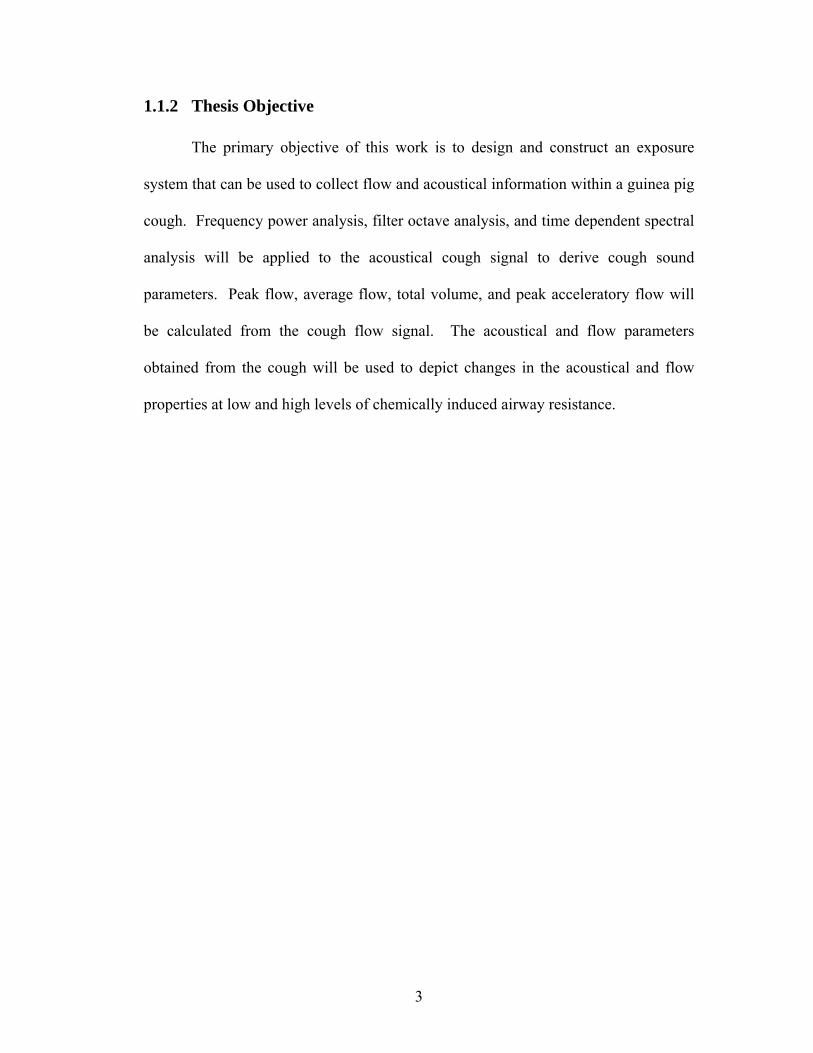
1.1.2 Thesis Objective The primary objective of this work is to design and construct an exposure

system that can be used to collect flow and acoustical information within a guinea pig

cough. Frequency power analysis, filter octave analysis, and time dependent spectral

analysis will be applied to the acoustical cough signal to derive cough sound

parameters. Peak flow, average flow, total volume, and peak acceleratory flow will

be calculated from the cough flow signal. The acoustical and flow parameters

obtained from the cough will be used to depict changes in the acoustical and flow

properties at low and high levels of chemically induced airway resistance.

3

Chapter 2 – Review of Relevant Literature

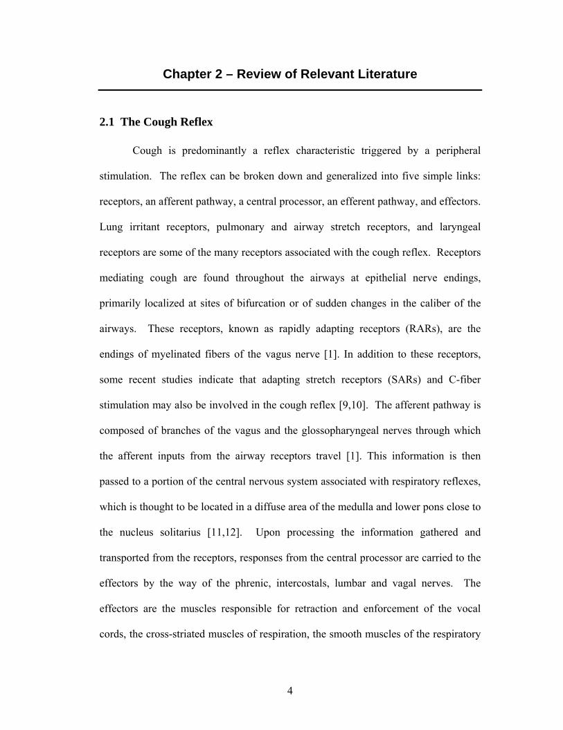
2.1 The Cough Reflex

Cough is predominantly a reflex characteristic triggered by a peripheral

stimulation. The reflex can be broken down and generalized into five simple links:

receptors, an afferent pathway, a central processor, an efferent pathway, and effectors.

Lung irritant receptors, pulmonary and airway stretch receptors, and laryngeal

receptors are some of the many receptors associated with the cough reflex. Receptors

mediating cough are found throughout the airways at epithelial nerve endings,

primarily localized at sites of bifurcation or of sudden changes in the caliber of the

airways. These receptors, known as rapidly adapting receptors (RARs), are the

endings of myelinated fibers of the vagus nerve [1]. In addition to these receptors,

some recent studies indicate that adapting stretch receptors (SARs) and C-fiber

stimulation may also be involved in the cough reflex [9,10]. The afferent pathway is

composed of branches of the vagus and the glossopharyngeal nerves through which

the afferent inputs from the airway receptors travel [1]. This information is then

passed to a portion of the central nervous system associated with respiratory reflexes,

which is thought to be located in a diffuse area of the medulla and lower pons close to

the nucleus solitarius [11,12]. Upon processing the information gathered and

transported from the receptors, responses from the central processor are carried to the

effectors by the way of the phrenic, intercostals, lumbar and vagal nerves. The

effectors are the muscles responsible for retraction and enforcement of the vocal

cords, the cross-striated muscles of respiration, the smooth muscles of the respiratory

4

system and the glands of the respiratory tract [1]. These five links work together to

process information and carry out the cough reflex.

The physical cough maneuver consists of a complex sequence of inspiratory

and expiratory efforts. The first phase is a preliminary inspiration of gas usually

larger than the normal breath [13]. At the end of the inspiration, the glottal adductors

close, the diaphragm relaxes, expiratory muscles contract, and the gas within the

lungs is compressed [14]. As the glottis reopens and an excitation of the

thoracoabdominal expiratory muscles occurs, the compressed air rushes from the

lungs periphery at a maximal flow rate [14,15]. In the final phase, known as the

cessation phase, muscle activity minimizes and airflow decreases to zero [16].

2.2 Human Cough Research

2.2.1 Sound Generation during Cough

Physicians have used pulmonary acoustics of various respiratory maneuvers to

help with the diagnosis of lung disease for many years. Although cough is often

considered to be a complication more so than a diagnostic tool, cough can also be

used in diagnoses [6,16]. It is important to understand the changes in cough sounds

due to lung disease. Cough sound is initiated by the flow of air through the large

airways of the lungs. The sound then travels through the upper respiratory tract,

through the oral cavity producing a broadband frequency signal, and out through the

lips. The sound that is produced provides important information regarding the sound

source and the filtering effects of the airways [8]

5

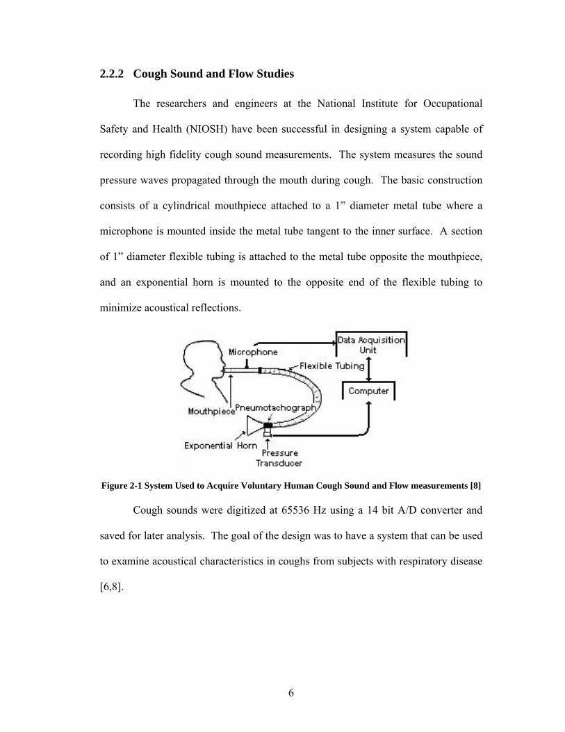
2.2.2 Cough Sound and Flow Studies

The researchers and engineers at the National Institute for Occupational

Safety and Health (NIOSH) have been successful in designing a system capable of

recording high fidelity cough sound measurements. The system measures the sound

pressure waves propagated through the mouth during cough. The basic construction

consists of a cylindrical mouthpiece attached to a 1” diameter metal tube where a

microphone is mounted inside the metal tube tangent to the inner surface. A section

of 1” diameter flexible tubing is attached to the metal tube opposite the mouthpiece,

and an exponential horn is mounted to the opposite end of the flexible tubing to

minimize acoustical reflections.

Figure 2-1 System Used to Acquire Voluntary Human Cough Sound and Flow measurements [8]

Cough sounds were digitized at 65536 Hz using a 14 bit A/D converter and

saved for later analysis. The goal of the design was to have a system that can be used

to examine acoustical characteristics in coughs from subjects with respiratory disease

[6,8].

6

Upon further investigation of the digitized signals obtained from the system in

Figure 2-1, distinct cough parameters were established. In one of the studies, a power

spectrum created from the cough waveforms showed that the cough waveform

exhibits a 1/fß relationship. By using a least square analysis to apply the closest

straight-line approximation of a log-log scale power spectrum, the exponent ß was

approximated to be equal to the slope of the straight line. Results show that there are

differences in ß between genders. This may be in part due to the differences in the

caliber or arrangement of airways between men and women [8]. Another useful

approach for analyzing cough waveforms is to view spectral information with respect

to time. A spectrogram visually displays frequency components by plotting

individual joint time-frequency color intensity blocks on a frequency versus time plot.

Wheezes, continuous or slowly changing tones, are visually evident by horizontal

bands of high intensity frequency components present in the spectrogram. Temporal

locations, frequency levels, and duration of the wheeze can be used to characterize

and diagnose different lung diseases [17].

Other studies focus on acoustic modeling theories to extrapolate information

from the free field measurement of a cough sound. Many of the theories are similar

to those applied in speech processing [5,18]. Van Hirtum et al used an auto-

regressive acoustical model, in which the current sample, ( )ty , is based on a finite

number, , of past samples an

( ) ( )ktyatyan

kkp −−= ∑

=1

ˆ

where is the predicted signal sample. ( )ty pˆ

7

The focus of this research was to determine frequency and bandwidths of

peaks in the spectra for human and animal coughs. Model order determination is

discussed and the ability to depict resonances within the cough is also explained [19].

Similar models, also based on speech processing algorithms, represent the respiratory

tract as a transfer function to model changing airway sizes as time varying diameter

changes in lossless tubes. Findings from this research indicate that it may be possible

to determine whether the cough sound can be used to reconstruct the respiratory tract

areas and distinguish between healthy individuals and those with chronic pulmonary

disease [5].

Cough flow characteristics have also been productive in determining

differences between healthy individuals and those suffering from obstructive lung

disease. Decreased peak flow, average flow, and peak acceleratory flow during

cough are indicators of obstructive lung disease. It has also been shown that men and

women exhibit different flow characteristics due in part to the arrangement and size

of their airways, further supporting the notion that flow characteristics provide insight

to actual construction of the airways [16]. By examining cough flow in conjunction

with acoustical properties, the intensity and duration of the cough can more

accurately be determined [7].

2.3 Guinea Pig Cough Research Cough spectral analysis, cough sound models, and flow characteristics

demonstrate great potential in obtaining distinct cough parameters in humans.

Despite significant progress in human cough research, research is limited by the

ability to conduct human exposures to certain occupational aerosols due to the

8

potential health hazards. For this reason, it is important to find an appropriate animal

substitute that exhibits many of the same responses to a wide variety of aerosols.

Animal studies have been conducted to estimate human pulmonary physiology for

quite some time. For the validity of this research it is important to show human and

guinea pig respiratory correlations. Using an animal with similar pulmonary

responses to humans is the first step in creating an accurate animal cough model.

2.3.1 Occupational Irritants

In many different occupational environments, gasses, vapors, and particles can

act as respiratory irritants [30]. These irritants can be classified as either sensory or

pulmonary irritants. Sensory irritants stimulate the unmyelinated C-fibers of the

trigeminal nerve endings located in the nasal mucosa [31,32]. In contrast, the

pulmonary irritants stimulate the vagal afferents either directly or through

inflammation in the conducting airways and alveoli. In guinea pigs and humans,

pulmonary irritants cause a decrease in tidal volume resulting in an increase in

breathing rate [20]. The effects of occupational irritants in test animals versus

humans reflect correlations between pulmonary inflammation responses and evidence

to the appropriate animal for this model. Table 2-1 is a collection of exposure results

illustrating the amount of pulmonary inflammation to a variety of occupational

irritants.

9

Table 2-1 Pulmonary Inflammation in Response to Inhalation of Various Gases, Vapors and Particles [20]

Agent Exposure Species PMN Cotton Dust 0 guinea pig 0.46±0.04 x 107 cells/gp 35 mg/m3; 2h guinea pig 4.00±1.23 x 107 cells/gp 0 rat 0.08±0.01 x 106 cells/rat 35 mg/m3; 6h rat 4.47±1.00 x 106 cells/rat Burnt hay 0 guinea pig 0.10±0.01 x 107 cells/gp 11 mg/m3; 6h guinea pig 1.50±0.50 x 107 cells/gp Chopped hay 0 guinea pig 0.33±0.03 x 107 cells/gp 6 mg/m3; 6h guinea pig 2.66±0.60 x 107 cells/gp Silage 0 guinea pig 0.20±0.02 x 107 cells/gp 8 mg/m3; 6h guinea pig 4.33±0.66 x 107 cells/gp Leaf/Wood Compost 0 guinea pig 0.42±0.10 x 107 cells/gp 30 mg/m3; 4h guinea pig 5.59±0.84 x 107 cells/gp Endotoxin 0 guinea pig 0.08±0.03 x 107 cells/gp 4x104 EU/m3; 3h guinea pig 3.31±0.69 x 107 cells/gp FMLP 0 guinea pig 0.15±0.01 x 107 cells/gp 1 mg/m3; 4h guinea pig 1.38±0.35 x 107 cells/gp 3-Glucan 0 guinea pig 0.30±0.02 x 107 cells/gp 23 mg/m3; 4h guinea pig 3.72±0.57 x 107 cells/gp Leather conditioner 0 guinea pig 0.17±0.06 x 107 cells/gp 2.5 mg/m3; 4h guinea pig 0.92±0.39 x 107 cells/gp Asphalt fume 0 rat 1.25±0.01 x 106 cells/rat 20 mg/m3; 4h rat 0.79±0.06 x 106 cells/rat Ozone 0 rat 0.40±0.04 x 105 cells/rat 2ppm; 3h rat 3.30±1.10 x 105 cells/rat

In guinea pigs, the polymorphonuclear leukocytes (PMN) obtained by

bronchoalveolar lavage peaks between 12 and 18 hours after the exposure. Similarly,

workers exposed to these aerosols exhibited a similar time course of inflammation

[20].

2.3.2 Citric Acid Cough Studies

Citric acid has been widely used to chemically induce cough in both humans

and other animals [21]. The cough reflex in the rat and mouse are less documented;

only chemical stimulation can induce the cough reflex, and the resulting coughs are

neither reproducible nor stable [1]. In a study conducted by Tartar and Pecova, the

10

sensitivity of the cough reflex in laboratory animals was tested. They found that

citric acid induced cough in 42.9% of unanethesized rats, 61.1% of rabbits, and 100%

of the guinea pigs [22]. While examining the role of partial laryngeal denervation on

the cough reflex in laboratory animals, results indicated that all guinea pigs tested,

50% of the rats, and 50% of rabbits coughed. Multiple studies by others have

produced similar results confirming that guinea pigs have a more sensitive cough

reflex than other laboratory animals [23].

The citric acid cough response in guinea pigs has also been proven similar to

that of humans. In a comparative study of a cough challenge with humans and guinea

pigs, both species exhibited similar dose dependant response curves.

Figure 2-2 Guinea Pig Log-dose-response Curves for Citric Acid and Capsaicin [21]

Figure 2-3 Human Log-dose-response Curves for Citric Acid and Capsaicin [21]

11

In Figures 2-2 and 2-3, the citric acid (-x-) and capsaicin (-●-) dose response

curves are plotted for guinea pigs and humans. The points show mean (±SEM) cough

frequency for each particular dose. The concentration-response relationship is

comparable in both subjects [21].

2.3.3 Methods of Recording Coughs in Guinea Pigs

A variety of methods have been used to record cough in guinea pigs. In most

studies, the intent was not to examine the contents of the cough sound but as a way to

ensure that coughs were being counted accurately. Scientists have mainly focused

their studies on the receptors and afferent pathways responsible for inducing cough

using a variety of cough inducing agents [1,24,33,34]. Counting coughs accurately

with a high certainty is a fundamental component in their research. Visually

observing coughs proved to be subjective and provided controversial information.

Using a microphone either built into the cage or attached to the animal provided a

more concrete basis for counting coughs. Despite these early efforts to quantify the

cough response, visual conformation of cough attempts proved essential to

differentiate coughs from sneezes or growls. Other methods involved measuring

changes in interpleural and tracheal pressure. This approach seemed to provide the

best evaluation of quality and quantity of cough [1].

2.3.4 Cough and Bronchoconstriction In recent studies, a common experimental protocol has been adopted for

guinea pig cough challenges. Forsberg uses this protocol in a study focusing on

cough and bronchoconstriction mediated by capsaicin-sensitive sensory neurons [24].

12

Initially, guinea pigs were placed individually in a Perspex chamber. They were then

exposed to nebulized citric acid, nicotine, and capsaicin for up to 7 minutes in

individual trials. Aerosols were produced by an ultrasonic nebulizer at a rate of

0.5mL/min, and two trained observers watched the animals and listened to amplified

sounds in order to accurately denote coughs. The two observers reported 0.39M citric

acid produced 6±3 and 5.8±3 coughs respectively in the first 3 minutes. The

bronchoconstriction reflex was defined as the development of a slow labored

breathing with exaggerated abdominal movements. The onset of bronchoconstriction

correlated in time with greatly altered breathing patterns, recorded on a Grass

polygraph, and a pronounced wheeze. The two observers reported the onset occurred

after 199±59 seconds and 199±57 seconds respectively. Figure 2-4 denotes the dose-

dependent response curves of citric acid in guinea pigs.

Figure 2-4 Guinea Pig Cough and Bronchoconstriction Dose Dependent Plots [24]

In this study, the onset of bronchoconstriction appeared to be independent of

the cough response. It was noted that during some cough challenges, coughs

13

occurred before bronchoconstriction and in others bronchoconstriction occurred prior

to coughs [24]. Based on these findings, the afferent pathways triggering broncho-

constriction seem to be different than those that trigger cough [25]. These results, and

other similar studies, have shown that citric acid induces cough and increases overall

lung resistance in anaesthetized guinea pigs [26,27].

To summarize, citric acid had similar effects in humans and guinea pigs. Its

provoked response seems to involve many of the same receptors and produce a

similar cough response. Citric acid has been shown to cause bronchoconstriction and

that the onset is unrelated to the cough response. This characteristic makes it possible

to monitor the specific airway resistance created by reflex bronchoconstriction and to

compare changes in the acoustical and flow characteristics at different stages of

bronchoconstriction. Measuring the constrictive effects of citric acid on the airways

while recording cough sounds will give insight into how the airway alterations change

cough characteristics in guinea pigs. Findings in this data may indicate that coughs

occurring after exposures to various occupational irritants can be measured and

characterized in a similar fashion.

14

Chapter 3 – Materials and Methods

The development of an animal model for studying cough sound and flow

measurements must meet several essential requirements. First and foremost, an

appropriate animal must be chosen for the cough challenges. In addition, an exposure

system must be developed to generate cough-inducing aerosols in a controllable

fashion. Following an exposure, the system must also be capable of simultaneously

recording cough sound and cough airflow measurements. Breathing pattern

measurements must also be saved to calculate specific airway resistance at the time of

the cough. It is essential that all data be saved so that synchronized measurements

can be obtained during an experiment.

3.1 Animal Considerations

Based on previous studies, guinea pigs appear to be a suitable choice for an

animal model. They are known to cough in response to irritants such as citric acid

and capsaicin. They provide more consistent and reproducible coughs than rats and

mice, and they have the advantage that they been used in many respiratory studies to

approximate human respiratory system responses. Furthermore, they exhibit a cough

response similar to that of humans.

The following protocol was used prior to exposing animals to conduct a cough

challenge. Male Hartley guinea pigs were allowed to acclimate to their new

environment for one week. After acclimation, they were loaded into the dual

chamber plythesmograph used during the exposures for a minimum of three

consecutive days to further acclimate them to the test environment. Once the smallest

15

guinea pig reached 300 grams, exposures began. This would allow approximately 10-

12 days for testing before the animal grew too large for the plythesmograph.

3.2 System Hardware

The animal cough system is a multifunction apparatus. It is used both to

expose the guinea pig to citric acid aerosols and record all cough sound and flow

measurements after the exposure. A diagram of the complete system is shown in

Figure 3-1.

Figure 3-1 Block Diagram of Exposure and Cough Recording System

16

3.2.1 Citric Acid Exposure Components

Citric acid aerosols were created using a Devilbiss Ultra-Neb 99 nebulizer. In

order to estimate the size and amount of aerosols present during the exposure,

preliminary aerosol diameter and concentration measurements were obtained using a

TSI model 3320 Aerodynamic Particle Sizer (APS) in the configuration shown in

Figure 3-2. The APS measurements are taken from the aerosols present within the

collection flask. The flask had a similar volume to that of the head chamber and was

used to simulate the space present within the head chamber.

Figure 3-2 Diagram of System Used to Measure Nebulizer Aerosol Size Distribution

The APS draws a constant flow of 5L/min through the system. A flow

calibrator (BIOS DryCal DC-Lite) was connected inline between the HEPA filter and

nebulizer to accurately measure the nebulized airflow. By adjusting the valve

between the intersection of the nebulized airflow and dilutant airflow and the lower

HEPA filter, the nebulized airflow could be altered. Figure 3-3 is a plot of the

measurements taken in a 30 second test period with a nebulized airflow of 0.35L/min.

Based on the obtained data, 67% of the citric acid aerosols were less than 2.5um and

95% of the aerosols are less than 10um in size.

17

0

2000

4000

6000

8000

10000

12000

14000

Part

icle

Cou

nt

<0.523 0.723 1.037 1.486 2.129 3.051 4.371 6.264 8.977 12.86 18.43

Aerodynamic Diameter (um)

Particle Count vs. Aeordynamic Diameter

Figure 3-3 Aerosol Generation for the Devilbiss Ultra-Neb 99 Nebulizer

When animals were exposed, the aerosols were delivered to the head chamber

by flowing air through the nebulizer cup using a 0-5L/min Aalborg mass flow

controller. A controllable dilutant air source was provided by a 0-10L/min Aalborg

mass flow controller. Using both mass flow controllers, the aerosol concentration

within the chamber can be increased or decreased rapidly at any time by remotely

adjusting the flow rates using the developed software. Each mass flow controller is

equipped with a 0-5V analog output indicating the flow rate and a 0-5V analog input

used to set the desired flow rate. Flow rates are determined based on a linear

relationship between voltage and flow. Hence, a 0V input results in no flow and 5V

input corresponds to the maximum flow rate for the particular flow controller.

Complete specifications for the mass flow controllers can be found in Appendix A.

Lastly, to insure proper oxygen exchange during all testing procedures, a 0-2.5L/min

Buxco bias flow vacuum pump was connected to the head chamber using 1/16” inner

diameter tygon tubing to pull air into the chamber at a constant rate of 1.2L/min.

18

3.2.2 Cough Flow and Sound Measurement Devices

The dual chamber plythesmograph (Hugo Sachs Elektronik-Harvard

apparatus) was equipped with screen type pneumotachs in both the head and thorax

chambers. See Figure 3-4. The resistances of the screens remain constant so that

airflow is directly proportional to chamber pressure, making it possible to measure

airflow into and out of each chamber. An in-depth description of how the flow

measurement was obtained from the pressure changes can be found in section 3.3.2.

To measure the pressure changes, Setra model 239 differential pressure transducers

are connected to each chamber. The pressure range for each transducer was -0.25 to

+0.25 inches of water. The output voltage ranges from –2.5 to +2.5V and follows a

linear relationship to pressure. See Appendix A for detailed specifications of the

pressure transducers.

PNEUMOTACHS

MIC/PREAMP

PRESSURE TRANSDUCERS

Figure 3-4 Digital Photograph of Dual Chamber Plythesmograph

19

Sound pressure waves were recorded using a Larson Davis audio setup

consisting of: a model 2530 pressure and random incidence ¼” microphone,

PRM910B ¼” preamplifier, and a 2200C dual channel microphone preamp/power

supply. The microphone was located in the head chamber approximately ½” from the

mouth of the guinea pig during the experiment. See Figure 3-4. The frequency

response of the microphone was 4Hz - 80kHz, making it ideal for recording high

frequency data. The microphone was matched with the preamp that was optimized

for use with the precision condenser microphone. The microphone was powered by a

2200C dual channel preamp/power supply which offers attenuation and gain settings

from –40 to +40dB relative to the input signal. The preamp/power supply furnishes a

microphone polarization voltage setting of 28Vdc to properly match the microphone

and conditions where it will be used. Outputs as high as 10Vrms are attainable for

frequencies up to 50kHz, and the unit holds a long-term constant calibration level for

changes in temperature and humidity. Refer to Appendix A for complete

specifications of the audio equipment.

3.2.3 Data Acquisition System Overview

All devices were controlled by one of two Data Acquisition (DAQ) cards. A

schematic of the complete DAQ system is shown in Figure 3-5. The National

instruments (NI) 6036E DAQ card is a low cost multifunction DAQ card. The card

features 2 analog outputs, 16 analog inputs with 16-bit resolution, and a peak

sampling rate of 200 kS/s. Complete channel access is made possible via the NI SC-

2345 signal conditioning box. The NI PCI-4451 DAQ card was selected for all audio

acquisition. The card features 2 16-bit simultaneously sampled analog inputs with

20

sampling rates from 5 to 204.8kS/s, and 2 analog outputs. The appealing feature

about this particular card is that all analog inputs have hardware implemented analog

and digital filters. Input signals pass through the fixed analog filters to remove

frequencies greater than the analog to digital converter’s range. The digitized signal

then passes through digital antialiasing filters that automatically adjust their cutoff

frequency to remove frequency components above half the sampling rate. Complete

specifications for these cards are located in Appendix A.

Figure 3-5 Electrical System Schematic

The NI 6036E DAQ is responsible for all data transfer to and from the

pressure transducers and air flow controllers. See Figure 3-5. Pressure transducer

analog outputs are first sent through a gain and offset adjustment box using a DB-9

connector. The gain and offset adjustment box is used to negate any DC offsets

21

found in the pressure signals. The box is also connected to a 24V battery to provide

the required excitation voltage for the pressure transducers. The airflow controllers

are connected to a junction box that powers both controllers and separates the analog

input and analog output signals. The DC zeroed pressure transducer signals and the

measured mass airflow readings are passed through a 4th order 50Hz low pass

Butterworth filter (SCC LP02) located within the signal condition box. The filter

eliminates any noise readings greater than 50Hz from the signals and prevents

frequencies greater than the cutoff frequency from being aliased as lower frequencies.

The air flow controller analog inputs, used to set desired flow rates, are connected to

analog output channels 0 and 1 of the NI 6036E DAQ card using the feed through

connectors (SCC FT01) located inside the signal conditioning unit.

All sound measurements are recorded using the high fidelity NI PCI-4451

DAQ card. This DAQ card is mated to the BNC 4451 for access to the 2 analog

inputs and 2 analog outputs provided on the card. The microphone/preamplifier

combination is connected to the 2200C power supply using a 5-pin Switchcraft

connector. The 2200C preamp/power supply amplifies the recorded sound pressure

voltage from the microphone by 40dB before outputting the signal. As can be seen in

Figure 3-5, channel 1 analog input is tied to the head chamber pressure signal. Since

analog inputs are read simultaneously, this allows synchronized cough sound and

flow measurements to be taken. Head chamber pressure signals recorded on channel

1 of the PCI-4451 DAQ card can then be correlated to the input from channel 0 of the

NI 6036E DAQ card. Thorax pressure recorded using channel 8 of the NI 6036E

DAQ card can be referenced to the recorded head chamber pressures recorded on

22

channel 0, enabling accurate synchronization of all flow and sound data. Complete

specifications for both DAQ cards are located in Appendix A.

3.3 Development of LabVIEW Data Acquisition Code

National Instrument’s LabVIEW 6i was the chosen software platform to meet

the data acquisition requirements for the above system. LabVIEW is a visual

programming language used to create virtual instruments (VIs) capable of controlling,

monitoring, and saving all inputs and outputs of the system. It is compatible with

both DAQ cards and has a broad range of configurable options. The following

sections will discuss the LabVIEW VIs developed for calibration and data

management.

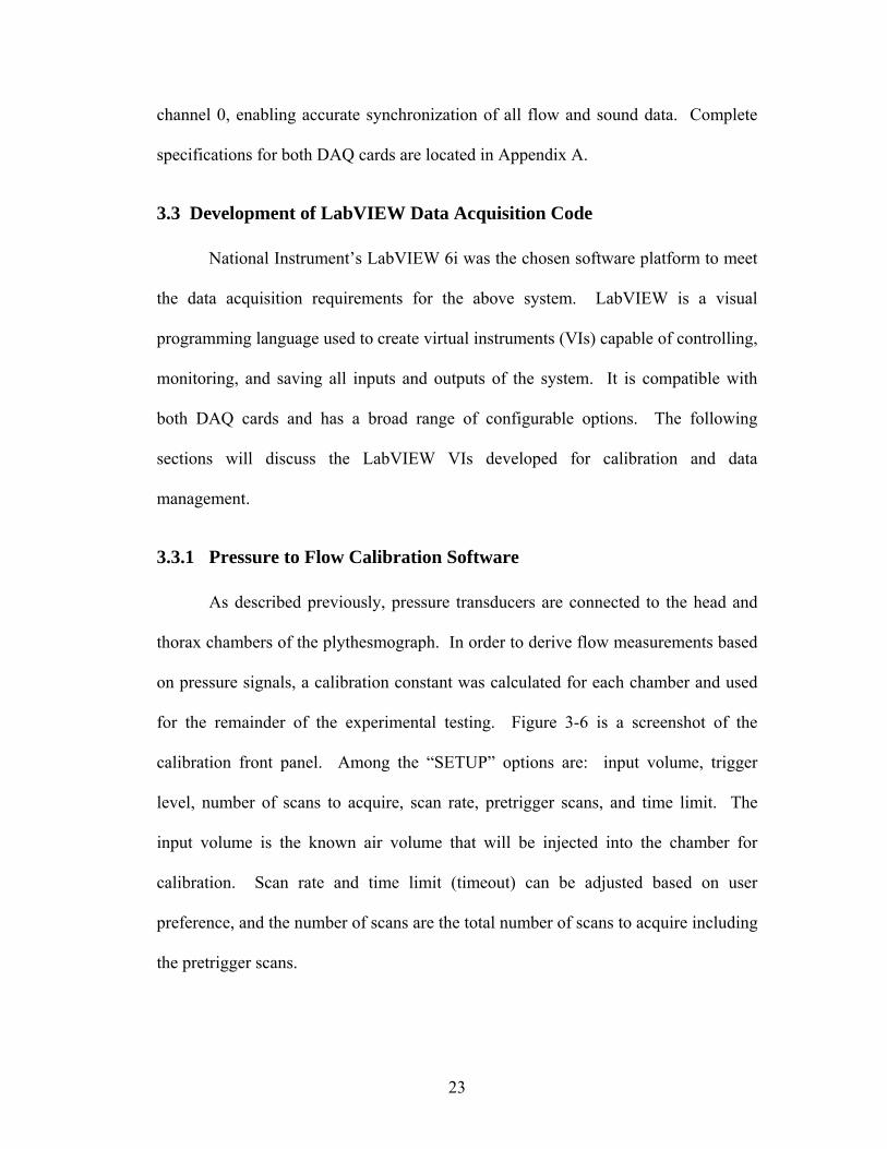
3.3.1 Pressure to Flow Calibration Software As described previously, pressure transducers are connected to the head and

thorax chambers of the plythesmograph. In order to derive flow measurements based

on pressure signals, a calibration constant was calculated for each chamber and used

for the remainder of the experimental testing. Figure 3-6 is a screenshot of the

calibration front panel. Among the “SETUP” options are: input volume, trigger

level, number of scans to acquire, scan rate, pretrigger scans, and time limit. The

input volume is the known air volume that will be injected into the chamber for

calibration. Scan rate and time limit (timeout) can be adjusted based on user

preference, and the number of scans are the total number of scans to acquire including

the pretrigger scans.

23

Figure 3-6 Calibration Software Virtual Instrument

In the present configuration, an air volume of 10mL is injected into the

chamber using a 10mL syringe. The airflow created from the air being added to the

chamber causes the voltage in the corresponding pressure transducer to increase.

When the pressure transducer output voltage exceeds 0.1V, the implemented software

trigger retrieves one second of previous buffered data and an additional four seconds

after the trigger, insuring the entire pressure signal is captured. The captured data is

sent to the conditional box (labeled as True) located in the center of Figure 3-7.

Twenty pretrigger samples are averaged to calculate the DC offset in the signal. The

offset is then subtracted from the original signal before any further calculations are

made.

24

The calibration constant and flow rate can be solved using Ohm’s law by

modeling the pressure, flow, and resistance of the calibration screens as a simple

resistor circuit. Relating Ohm’s Law to Pressure:

))(( screenRFlowPIRV

=∆=∆

(1)

screenRPFlow ∆

= (2)

∫ ∫∆

=screnRPFlow (3)

(4) VolumeFlow =∫

screenR

PVolume ∫ ∆= (5)

Volume

PRscreen

∫ ∆= (6)

screenRCC =1 (7) where CC is the calibration constant

Therefore,

∫ ∆

=P

VolumeCC (8)

As can be seen in upper right portion of Figure 3-7, equation 8 is used to

calculate the calibration constant. In a series of three tests, CC was 50±3 in each

chamber. The input volume is divided by the integrated pressure signal (the output

from the conditional statement). The flow curve is calculated by taking the product

of the pressure change and the derived calibration constant. The volume curve is

calculated by integrating the pressure signal and multiplying it by the calibration

constant. The resulting flow and volume curves after the calibration test are shown in

Figure 3-8.

26

Figure 3-8 Calibration System Output

3.3.2 Front Panel Design and Operator Interface Description The “Gpig Cough and Flow” VI, shown in Figure 3-9, is the next software

component in the data acquisition system. This VI was created to control and

monitor the citric acid exposure devices and the store relevant breathing, cough

sound, and cough flow data obtained during the testing procedure. Before starting the

software, the initial desired dilutant and nebulized airflows are set to zero. The head

and thorax calibration constants, calculated from the calibration VI described earlier,

are entered into the appropriately labeled text boxes located under the filtered cough

plot area. At any time once the VI is started, head and thorax calibration constants

can be recalculated by pressing the corresponding buttons located on the far left.

27

Figure 3-9 Exposure and Cough Acquisition Front Panel

After entering the needed inputs, the program can be started by pressing the

small white arrow below the menu bar. As soon as the program starts, a dialog box is

displayed requesting the user to input the date and guinea pig identification number

used for the current exposure. See Figure 3-10.

Figure 3-10 Directory Setup Dialog Box

28

Date and guinea pig information is used to create a directory structure and

assign filenames for the data acquired during the exposure. Data content within each

of the saved files is saved in a binary format to conserve disk space. Using the

information entered in Figure 3-10, the following files would be created and opened

for writing within the C:\09-13-03\gpig5\ directory.

• flowconc.fc5 – This file contains the raw voltage signals from both pressure transducers from the start of the exposure until the stop button is pressed. A header is written to the file containing the date, time, and length of the exposure. Also included in the header are the calibration constants, sampling rate (4000/S/s), and the text entered in the “FILE COMMENTS” in Figure 3-9.

• sound.base5 – This file contains a sample baseline sound file of the first 20

seconds of the exposure while the dilutant and nebulized airflows are turned off and the animal is in the chamber. In the post processing stage, this file will be used as a reference noise baseline. Header file includes date, time, sampling rate (98304S/s), and “FILE COMMENTS.”

• cough###.dat – These files are 1 second sound files saved during the exposure

when a potential cough occurred. (Cough detection will be explained in greater detail later in this section) The header of these files includes: date, time, sampling rate (98304S/s), elapsed time, and the acquisition backlog. File numbers begin at 1 and are incremented as potential coughs are recorded.

• flow###.dat – These are the corresponding flow files recorded from the head

chamber. They contain the same header information as the sound files and are sampled at the same rate.

After the date and guinea pig information is entered and the user presses the

“DONE” button, the designated filenames are displayed on the front panel. Pressure

signals in the head and thorax chamber are converted to flow rates and updated to the

front panel approximately every 0.15 seconds. See Figure 3-11. Dilutant and

nebulized airflows can be changed at any time during the exposure by typing in the

desired flow rates, or by using one of the two buttons located in the lower left

position of the front panel labeled “FLUSH CHAMBER” and “STOP FLOWS.”

29

Figure 3-11 Exposure and Cough Acquisition Front Panel Displaying Measured Flow Rates

While the thorax and head flow rates are being displayed and recorded in the

flowconc.fc# file, data from both channels of the PCI-4451 DAQ card are being

sampled. As noted earlier, channel 0 corresponds to the microphone signal and

channel 1 is the pressure in the head chamber. Each channel is read using a series of

prepackaged LabVIEW analog functions. Analog input functions were configured to

sample at 98304 S/s and store data into a 196608 sample (2 second) buffer. All data

within the buffer is read and cleared by an analog read executed in the main loop of

the program. The inputs from both channels (labeled as Sampled data in Figure 3-12)

are parsed and recorded in separate circular buffers, each 1 second (98304 samples) in

length.

30

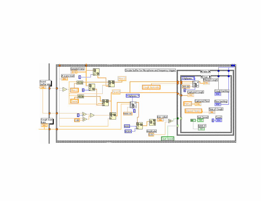
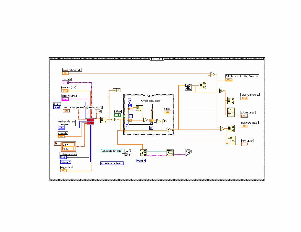
A specialized software trigger was created to examine the sound data to

determine if a cough occurred. The trigger is designed to look at the samples located

in the middle of the sound buffer and determine if frequencies above 5000Hz exceed

an amplitude of 0.01V. In Figure 3-12, the position of the first sample of the data to

be examined is obtained by dividing the buffer in half and subtracting half of the

number of scans read each time through the loop. The last sample in the data is the

position of the first sample plus the number of samples read during a single read

process. This segment of buffer is sent to an 8th order 5kHz high pass Butterworth

filter. The max value of the output from the filter is compared to the desired

amplitude. If the recorded sound exhibits frequency components greater than 5kHz

and data was not stored from the buffer one read cycle earlier, the conditional

statements on the far right are executed. Inside the conditional statements, the entire

unfiltered sound buffer (labeled as Sound) and the corresponding flow buffer (labeled

as Flow2) are saved. The unfiltered data in the cough buffer is then filtered using an

8th order 300Hz high pass Butterworth filter and the resulting cough waveform is

plotted in the front panel as shown in Figure 3-13. The cough and cough flow files

are incremented and the system is ready to record the next cough.

32

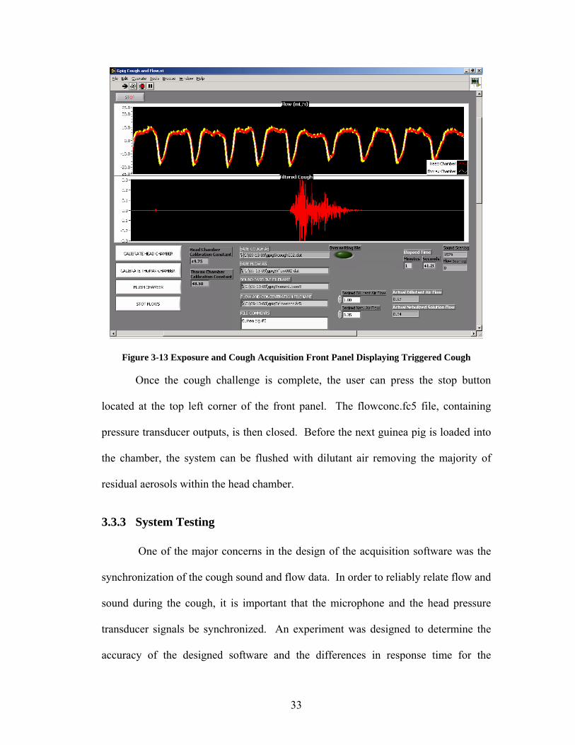
Figure 3-13 Exposure and Cough Acquisition Front Panel Displaying Triggered Cough

Once the cough challenge is complete, the user can press the stop button

located at the top left corner of the front panel. The flowconc.fc5 file, containing

pressure transducer outputs, is then closed. Before the next guinea pig is loaded into

the chamber, the system can be flushed with dilutant air removing the majority of

residual aerosols within the head chamber.

3.3.3 System Testing One of the major concerns in the design of the acquisition software was the

synchronization of the cough sound and flow data. In order to reliably relate flow and

sound during the cough, it is important that the microphone and the head pressure

transducer signals be synchronized. An experiment was designed to determine the

accuracy of the designed software and the differences in response time for the

33

microphone and the head chamber pressure transducer. In order to do this, a small

inflated balloon was placed in the head chamber and pricked. The sound and flow

data were examined to ensure that the sound and flow measurements were in phase.

In a series of three tests, the pressure transducer had an average delayed response of

108 samples resulting in a .0011 second slower response time.

3.4 Experimental Procedure Two groups of six guinea pigs were used for the exposures. Nebulized

airflows and exposure stopping criteria were determined based on preliminary cough

challenges. See Table 3-1. The goal of the preliminary testing was to generate

exposure guidelines for triggering coughs at different levels of bronchoconstriction.

In order to minimize bronchoconstriction and consistently trigger the cough response,

the nebulized airflows were set between 0.3 and 0.35L/m and the exposure was halted

immediately after the first cough effort. By increasing the nebulizer airflow and

delaying measurements until the second cough, the onset of bronchoconstriction was

thought to occur earlier with an increased effect, thus producing coughs with

increased airway resistance. As indicated in Table 3-1, three of the six guinea pigs in

each group were exposed to ozone for three hours at a aerosol concentration of 2ppm

before the third day of the scheduled citric acid exposures. Ozone has been shown to

increase airway resistance up to three hours post exposure and to slightly decrease

airway resistance thereafter [35]. The ozone exposure, in combination with varying

nebulizer airflow settings and stopping criteria, enabled cough data to be collected

with an increased variance in airway resistance.

34

Table 3-1 Guinea Pig Exposure Parameters and Stopping Criteria

Days from Initial Elapsed Time since Nebulized Airflow Exposure Citric Acid Exposure Ozone Exposure (L/min) Stopping Criterion

0 NE 0.3 - 0.35 First Cough Effort (n = 12)

1 NE 0.35 - 0.4 Second Cough Effort or (n = 12) Evident Bronchoconstriction

2 NE 0.3 - 0.35 First Cough Effort (n = 6)

2 ~ 15 min 0.3 - 0.35 First Cough Effort (n = 6) (c = 3 hours @ 2ppm)

3 NE 0.3 - 0.35 First Cough Effort (n = 6)

3 18 hours 0.3 - 0.35 First Cough Effort (n = 6) (c = 3 hours @ 2ppm)

7 NE 0.35 - 0.4 Second Cough Effort or (n = 6) Evident Bronchoconstriction

7 5 days 0.35 - 0.4 Second Cough Effort or (n = 6) (c = 3 hours @ 2ppm) Evident Bronchoconstriction

c = ozone exposure level

n = number of animals studied

NE = not exposed

Before conducting each exposure, all airflows were turned off and a

calibration stopper was placed in the removable cylinder of the plythesmograph to

provide an airtight seal between the head and thorax chamber. DC offsets from the

pressure transducers were zeroed using the gain and adjustment offset box in

conjunction with the test panel in the NI Measurement and Automation software

package. Calibration coefficients for each chamber were determined and any air

leaks in the system were remedied.

Upon successful calibration, a prepared 50mL solution of 0.39M citric acid

was placed into the nebulizer cup, and all test animals were weighed. Guinea pigs

35

were then loaded individually into the removable slotted tube of the plythesmograph

and positioned so that the flexible plastic seals fit snugly around the animal’s neck.

The removable tube and guinea pig were then placed horizontally into the

plythesmograph. For the remainder of the experiment, a constant flow of 1 liter/min

from the Buxco pump was provided to the head chamber. All valves remained

closed, and only the holes with the screens were open. This is the configuration in

which all acoustical and flow measurements were recorded.

Once the animal was relaxed inside the chamber, the data acquisition software

was started. Initial breathing measurements were taken during the first 20 seconds in

the current configuration. After the initial 20 seconds, the system was converted to

begin delivering citric acid aerosols to the head chamber of the plythesmograph. The

nebulizer was turned on, the exhaust valve and the nebulized/dilutant airflow valve

were opened, and the cap was placed in the head chamber opening to prevent citric

acid aerosols from leaking out of the head chamber. The nebulized airflow was set

based on Table 3-1, and the dilutant airflow was held constant at 1L/min throughout

the exposure. The citric acid exposure was stopped based on the criterion in

Table 3-1. Once the stopping criterion was met, the plythesmograph was then

reverted to the measurement phase described earlier with the cap removed from the

head chamber and all valves closed. Cough sound and flow data was recorded for up

to 10 minutes after the exposure. The guinea pig was then removed from the chamber

and the head chamber was flushed with dilutant air at a rate of 10L/min for 30

seconds.

36

Chapter 4 – Data Processing Methods

After acquiring data using LabVIEW and associated hardware, post

processing was performed in Matlab. Although LabVIEW is capable of real time

data processing, all data stored during the data acquisition process was saved in its

raw format for later analysis. The following chapter is an in-depth explanation of the

data extraction process and the methods used to generate the cough parameter

spreadsheet. The results from the data processing algorithms in this chapter will be

presented in Chapter 5.

4.1 Specific Airway Resistance

There are many methods used to estimate airway resistance [39, 41]. Specific

airway resistance (sRaw), a commonly used noninvasive airway resistance estimation

technique, uses dual chamber plythesmography [41]. In this analysis, sRaw (airway

resistance times thoracic gas volume) estimates airway resistance by assuming the

thoracic gas volume of the lungs remains fairly consistent throughout the exposure.

sRaw provides a metric for quantifying the aerosol-induced bronchoconstriction

present during each cough.

An efficient method was developed to estimate sRaw near the time of the

cough by analyzing the pressure changes across the screens in the head and thorax

chamber during guinea pig respiration. Using the recorded pressure changes, the

nasal and thorax flows can be calculated given the flow resistance of the screens in

each chamber. The flows entering and exiting the chambers as a result of the drive in

the thorax can be modeled as an electrical circuit (See Figure 4-1). Pressure (inches

37

of H2O) is analogous to voltage, current represents the flow of gas in mL/s, and

resistors are viewed as the resistance to flow in (inches of H2O)/mL/s.

Figure 4-1 Electrical Flow Model of Guinea Pig in the Dual Chamber Plythesmograph

PT and PH are the thorax and head chamber pressure readings recorded in the

flowconc.fc# file during the exposure. RST and RSH are the resistance of the screens in

each of the chambers, and CT and CH are the capacitance or compliance in

ml/inchH2O due to the volume present within the chambers. The current source D is

the flow created by the driving force of the guinea pig’s thorax. CG is the capacitance

of the thoracic gas volume present in the lungs, and Raw is the resistance of the

airways. By combining the resistance and capacitance in each chamber into a lumped

impedance, the circuit can be rewritten where ZT and ZH represent the combined

impedance of the screens and volume in each of the chambers. See Figure 4-2.

38

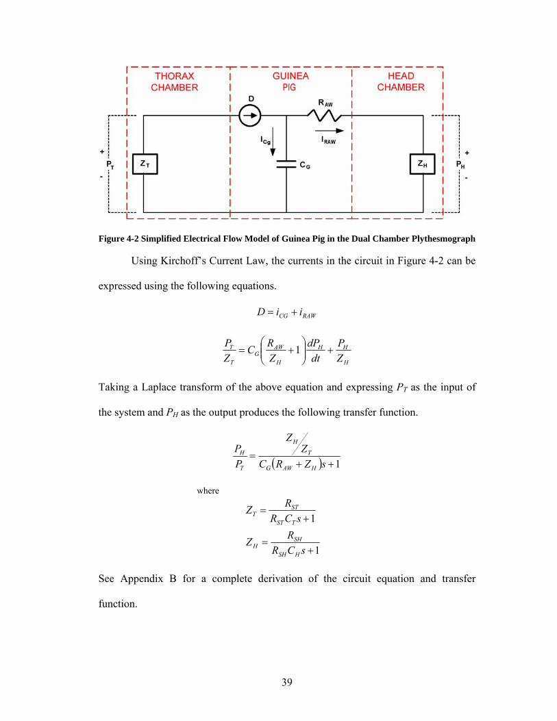
Figure 4-2 Simplified Electrical Flow Model of Guinea Pig in the Dual Chamber Plythesmograph

Using Kirchoff’s Current Law, the currents in the circuit in Figure 4-2 can be

expressed using the following equations.

RAWCG iiD +=

H

HH

H

AWG

T

T

ZP

dtdP

ZRC

ZP

+⎟⎟⎠

⎞⎜⎜⎝

⎛+= 1

Taking a Laplace transform of the above equation and expressing PT as the input of

the system and PH as the output produces the following transfer function.

( ) 1++=

sZRCZ

Z

PP

HAWG

T

H

T

H

where

1

1

+=

+=

sCRRZ

sCRRZ

HSH

SHH

TST

STT

See Appendix B for a complete derivation of the circuit equation and transfer

function.

39

The goal is to quantify how the change in specific airway resistance changes

the spectral components of the cough sound. Since the actual airway resistance is not

as critical to this analysis as is the change in airway resistance, the system transfer

function can be simplified based on the following assumptions. The first assumption

is that ZT and ZH are equal. The capacitance (change in volume/pressure) in each

chamber is assumed to be nearly equal since the chambers have similar volumes and

the pressure changes within the chamber are minimal. The resistance of the screens,

RSH and RST, as defined in Section 3.3.1 is the inverse of the calibration constant CC.

CC was calculated to be 50±3 mL/s·Volt in both chambers. The pressure transducer

voltage resolution is 0.1inchH2O/V. Therefore, the resistance of the screens can be

calculated as R in the following equation.

smLOHinch

sOinchHmL

sVmLCC

R/

002.1.0

501

5011 2

2

⋅=

⋅=

⋅==

By assuming both the capacitance of each chamber and the resistance in each

chamber are equivalent, then ZT ≈ ZH.

The second assumption is that the impedance in the head chamber, ZH is very

small in comparison to the resistance of the airways. Comparing airway resistance

measurements obtained by Pennock et al with the chamber airflow resistance

calculated above supports this assumption. Pennock found guinea pig airway

resistances at different stages of bronchoconstriction to range from 0.2 – 1.77

smLOinchH

/2 using a pleural catheter [41]. Since the resistance of the screen accounts

for <1% of the total resistance, the impedance (RAW + ZH) in the denominator of the

40

transfer function can be approximated as RAW. Following these assumptions, the

transfer function can now be expressed in terms of PT, PH, CG, and RAW.

11

+=

sCRPP

GAWT

H

Since PT and PH are synchronously recorded, CGRAW was determined in

Matlab using the least square fit algorithm by rewriting the transfer function in the

time domain.

)()()( tPdt

tdPCRtP TT

GAWH +⋅=

RAWCG was calculated by finding the coefficient that produced the least squared error

in the time domain expression of the transfer function. To evaluate the fit, the head

chamber flow (PH x CC), thorax chamber flow (PT x CC), and simulated flow from

the above equation was plotted as shown in Figure 4-3.

Figure 4-3 Head Chamber Flow, Thorax Chamber Flow, and Simulated Head Chamber Flow

41

Given that RAWCG = RAW · TGV/PB and sRaw = RAW · TGV, sRaw and can be

calculated from RAWCG by multiplying by the barometric pressure PB. Since the

change in RAWCG is equivalent to the change in sRaw, the correlation between cough

characteristics and airway resistance were made using the time constant between the

nasal and thorax breathing signal, RAWCG.

4.2 Acoustical Analysis

4.2.1 Data Extraction Matlab software was developed to read in all potential coughs saved during

the data acquisition process. Before developing cough statistics for each acquired

potential cough, the saved data was played at 1/6th the sampling rate to discriminate

between coughs, sneezes, growls, or other noises (animal movement, squeals, etc)

that may have inadvertently triggered the acquisition. Growls and noises were easily

distinguished from coughs and sneezes by playing the cough sound at a reduced

sampling rate. In most cases, coughs played at the reduced sampling rate sounded

similar to human coughs and were distinguishable from sneezes. Potential coughs

that could not be distinguished audibly were not included in the dataset. Ideally,

coughs would be correlated with known characteristics of a guinea pig cough to

classify the recorded data. However, there is no previous referenced work accurately

characterizing the acoustical waveforms of the guinea pig cough.

Each cough was saved in an appropriate directory with all other coughs

obtained during the exposure. The final step before analyzing the cough was to find

the beginning and the end of the cough. Figure 4-4 contains a plot of a cough in its

42

raw format and a filtered version obtained from an 8th order high pass 500Hz

butterworth filter.

Figure 4-4 Time Domain Representation of Guinea Pig Cough

Cough start and end points were based on the amplitude of the filtered cough

as indicated by the vertical red lines in the “Filtered Data” plot. The start and stop

times of each cough were saved in appropriately named binary MAT-files and the

cough length was recorded in the cough parameter spreadsheet. In the following

cough sound and flow analysis, the cough files were loaded with the corresponding

start and stop times, and only the data in the designated timeframe was analyzed.

43

4.2.2 Energy and Average Power

Since sound waves travel as waves of compression and rarefaction, sound

measurements are typically calculated based on the sound pressure level (SPL). SPL

is measured on a logarithmic scale in dB because sound pressures of various sounds

tend to cover large ranges [40]. In this analysis, sound energy and power levels were

calculated with standard signal processing equations by using the amplified voltage

signal from the microphone instead of the actual sound pressure level. Energy was

calculated from the time domain respresentation of the microphone voltage signal

using the following equation.

∑=

=N

nnxEnergy

0

2|)(|

The total energy of the signal was then divided by the sampling rate to convert energy

to a time based energy measurement. Average power was calculated using the

following equation [38].

∑=

=N

nnx

NPowerAvg

0

2|)(|1.

where N = the number of samples

x(n) = time domain cough sound

By calculating energy and power based on standard signal processing

equations, energy and power can be compared between coughs on a linear scale. The

primary reason calculations were made this way was to provide proportionally

weighted parameters since all other parameters were calculated on linear scales.

44

4.2.3 FFT

The fast Fourier Transform (FFT) is the mathematical basis of many of the

spectral analysis techniques used to analyze cough sound data. The primary function

of the FFT is to transform sampled data from the time domain to the frequency

domain. The FFT works on the basis that the signal is composed of a number of

sinusoidal components of various frequencies, amplitudes, and initial phases. The

resulting sinusoids are then summed creating a frequency domain signal. To analyze

discrete time signals, a variation of the FFT known as the discrete Fourier Transform

(DFT) is used. The defining equation is as follows:

∑∞

−∞=

−=n

ftjn

netgfG π2)()(

)( fG is the frequency domain representation of the time domain signal [36].

The DFT is the fundamental component in many of the data processing techniques in

the following sections.

)( ntg

4.2.4 Power Spectrum

The power spectrum is used to calculate the power as a function of the

frequency. Typically, a power spectrum analysis is more applicable to stationary

signals. Coughs are better described as non-stationary signals since the frequency

content changes throughout the cough. Although cough sounds are more

characteristic of non-stationary signals, it was assumed that they can be divided into

short quasi-stationary sections and analyzed as stationary signals [36]. In the analysis

of the cough sound, Welch’s method and Burg’s method were used to analyze the

45

cough power spectrum. Welch’s method is one of the more common methods used

for analyzing the frequency power relationship. While examining the power spectra

using Welch’s method, the power in adjacent frequencies appeared to be quite

oscillatory. Burg’s method was used to provide a smoother power spectrum and

capture the major characteristics. Cough parameters were derived using both power

spectrums.

4.2.4.1 Welch’s Method

The first step in Welch's method for estimating the power spectrum is to

divide the time signal into successive blocks. The process of sectioning the time

domain signal into smaller signals is called time windowing. Sliding the window

across the time domain signal and calculating spectral intensity for that window in

essence breaks the cough sound into stationary segments [36]. In the analysis of

cough sound data, a 256 sample Hanning window was used with an overlap of 128

samples or half the window size.

Before calculating the power spectrum from each window, the individual

windowed time domain signals were zero-padded by adding zeros to the time domain

signal. Zero-padding is a technique that is often used to interpolate between

frequency samples of a fixed length DFT and is effective in producing more

frequency samples of the periodically replicated signal spectrum. Since a true

improvement in spectral resolution can only be achieved using a longer time-duration

window, zero padding is a somewhat artificial method for improving frequency

resolution [38].

46

For each zero-padded time domain window, the spectral power using Welch’s

method was calculated by averaging the squared magnitude DFTs using the following

equation:

21

0|)(|1)( m

M

mk xDFT

MfPxx ∑

−

=

=

M denotes the number of windowed time samples and is the time domain signal

within the current segment. is the returned power spectrum estimate for the

complete signal [38]. The power spectrum for a randomly selected cough using

Welch’s method with a DFT length of 2048 samples is shown in Figure 4-5. The

frequency and magnitude corresponding to the highest peak in the cough spectrum

were recorded in the cough parameter spreadsheet as the dominant frequency and

peak power.

mx

)( fPxx

Figure 4-5 Welch’s Power Spectrum

47

4.2.4.2 Burg’s Method The Burg method calculates the spectral density from the frequency response

of an all-pole linear filter specified by the autoregressive (AR) linear prediction

model. The first step in generating the power spectrum using this method is to

calculate the coefficients of the following linear prediction model.

( ) ( )ktyatyn

kkp −−= ∑

=1

ˆ

The current sample , is predicted from a linear combination of a finite number of

past samples ( n ) yielding the predicted signal sample,

( )ty

( )ty pˆ . is the prediction

order, and is a vector of calculated model coefficients [19]. Using the least squares

method, the Burg method calculates the best fit model of the input signal by

minimizing the mean of the forward prediction error

n

a

( )tytyf pn ˆ)( −= and the

backward prediction error ( )ntyntyg pn −−−= ˆ)( where

( ) ( nktyantyn

kkp −+−=− ∑

=1

ˆ )

The resulting coefficients are constrained to satisfy the Levinson Durbin recursion

algorithm [38]. From the derived coefficients, the input data is characterized using a

source based all-pole transfer function, and can be written in the z-domain as

pp

q zazazaezH −

+−− +++

=)1(

23

12 ....1

)(

where e is the variance estimate of the input to the AR model.

The complex frequency response is calculated by evaluating at

and performing a DFT on the numerator and denominator. The numerator is divided

qH )( ωjez =

48

point by point by the denominator yielding the complex frequency response vector of

the prediction filter. The power spectrum is obtained from the product of the

estimated AR model variance and the complex frequency response vector. The

resulting power spectrum is shown in Figure 4-6 for the same cough as in Figure 4-5.

Figure 4-6 Burg’s Power Spectrum

The prediction model order has an important role in the frequency response of

the prediction filter, and is directly related to the number of poles in the filter transfer

function. The peaks in the power spectrum of Figure 4-6 correspond to frequencies

near the poles of the filter. In order to capture the main peaks of the power spectrum

and eliminate the small oscillatory peaks seen using Welch’s method, a 20th order

Burg model was selected. As can be seen in Figure 4-7, a 20th order model produces

a much smoother power spectrum while preserving the major characteristics.

49

Figure 4-7 Comparison between Welch’s Power Spectrum and Burg’s Power Spectrum

In order to use the power spectrum as a parameter or group of parameters for

correlating the cough sound spectrum with airway resistance, the peak power of the

spectrum was recorded in conjunction with a set of estimated power spectrum

parameters. Peak power was obtained from the maximum magnitude of the power

spectrum, and the estimated power spectrum parameters were calculated by dividing

the power spectrum into thirty-two 1500Hz non-overlapping frequency blocks and

averaging the power in each block. The peak power and the estimated power

spectrum parameters were saved in the cough parameter spreadsheet for later

analysis.

50

4.2.4.3 Octave Analyzer

The power spectra of both Welch’s method and Burg’s method were split into

seven octaves beginning at 500Hz. For a standard octave analyzer, the upper cutoff

frequency in each octave is twice the lower cutoff frequency [37]. Figure 4-8

demonstrates how the power spectrum was split into different octaves using Welch’s

power spectrum.

Figure 4-8 Octave Breakdown Using Welch’s Method

The percent power in each octave was calculated by dividing the power in

each octave by the total power in the signal. The octave analysis was performed on

the power spectra generated by both Welch’s and Burg’s power spectrum estimation

methods. All octave percent powers for both spectrums were saved in the cough

parameter spreadsheet.

51

4.2.5 Frequency vs. Time analysis 4.2.5.1 Spectrogram A spectrogram is a time-dependent frequency analysis technique used to

compare the cough spectrum with respect to time. The spectrogram splits the cough

sound into overlapping sections specified by the window size and the number of

samples each window is to overlap adjacent windows. For the cough sounds, a

window size of 128 samples with a 96 sample overlap provided the best overall time

(horizontal) and frequency (vertical) resolution. To calculate the short-term

frequency content of the signal, each window was zero-padded to a length 2048 and

the DFT was performed on each window. The color intensity in the spectrogram is

representative of the frequency power during the cough. See Figure 4-9.

Figure 4-9 Guinea Pig Cough Spectrogram

52

4.2.5.2 Spectrogram Parameters

The Matlab specgram function outputs vectors F and T, and matrix B.

Vectors F and T contain the range of frequencies and midpoint of the time window at

which the DFT is computed. B is a (length of F) x (length of T) matrix composed of

the frequency magnitude or power at F frequencies at T times.

To provide a quantitative feel of how the frequency or pitch changes during

the cough, two methods were developed for characterizing the spectrogram. The first

method calculates a weighted frequency average at different times during the cough.

The output vector T is divided into thirty equally sized time frames. For each

timeframe, F was multiplied by the corresponding frequency magnitudes found in B.

The product of F and B was divided by the total frequency magnitudes in each

respective timeframe; thus producing weighted average frequencies for all

timeframes. The resulting vector is transposed on the spectrogram in Figure 4-10.

Figure 4-10 Average Frequency Vector

53

The next method is similar to the previously described method, except the

weighted averaging is computed along the time axis. Instead of separating the cough

into timeframes, the cough spectrum is broken down into 30 non-overlapping

frequency bands. The product of the frequency power in each frequency band and T

were divided by the respective frequency power obtained from matrix B. The

resulting averages define the time at which the midpoint of the power occurs in each

frequency band during the cough. See Figure 4-11. The horizontal lines are the

frequency band divisions and the vertical lines are the power midpoint for each

frequency band.

Figure 4-11 Power Midpoint in Frequency Bands

54

4.3 Cough Flow Analysis

Peak flow, average flow, peak acceleratory flow, and total expiratory volume

parameters were calculated for all coughs. Flows were calculated by multiplying the

head chamber pressure signal obtained during the cough by the calibration coefficient

recorded in the header of each flow#.dat file. The maximum flow recorded during the

cough was noted as the peak flow. The average flow was calculated by a point-by-

point addition of all the flow values obtained during the cough divided by the total

number of points in the cough length. Peak acceleratory flow (mL/s2) was calculated

by finding the peak value in the derivative of the flow signal. The total expiratory

volume was calculated by integrating the flow signal for the duration of the cough.

4.4 Cough Characteristics vs. Airway resistance

Given the large number of cough parameters derived from the previously

described methods, a fast, reliable approach was needed to quantify the relationship

between the derived cough parameters and the time constant, RAWCG. The primary

goal of the analysis is to determine how accurately coughs occurring at a low airway

resistance can be distinguished from coughs occurring at a high airway resistance.

The approach taken was a two-step process. The first step was to re-express the

cough parameters through principal component analysis (PCA). The resulting cough

parameters were then weighted and summed using a single neuron neural network

thus providing a single output relating the cough sound to airway resistance.

Before processing the cough parameters, coughs were divided into three

groups based on the average of the pre-cough and post-cough RAWCG measurements.

Groups 1, 2, and 3 were categorized of having low, moderate, and high airway

55

resistances respectively. Outliers within each group where determined by calculating

the standard deviation of each parameter within the group. Coughs having 10% or

more parameters exceeding two standard deviations from the mean of the group were

considered poor coughs and removed from the dataset. This resulted in

approximately 9% of the coughs being removed in each group. The resulting group

statistics are in Table 4-1.

Table 4-1 Cough Group Statistics

Group # RC range (s) RC avg ± std (s) # of coughs 1 0.0040 - 0.0060 0.0051±.00053 113 2 0.0060 - 0.0095 0.0073±0.0010 143 3 0.0095 - 0.0154 0.0117±0.0016 93

Group divisions were established to force the airway resistance measurements

of group 3 to be approximately double that of group 1, while maintaining a

considerable number of coughs in both groups. Group 2 contains the coughs in the

transition from the low airway resistance coughs of group 1 to the high airway

resistance coughs of group 3. The following chapter will primarily focus on the

cough characteristics in groups 1 and 3 to discriminate coughs occurring at low and

high airway resistances. To properly insure that the proposed analysis focuses on

changes due to airway resistance and not the differences in cough characteristics of

the guinea pigs in each group, the number of guinea pigs representing coughs in each

group including the number of coughs exhibited by those guinea pigs were counted.

Coughs in groups 1 and 3 were both comprised of coughs from ten guinea pigs. Eight

of the ten guinea pigs exhibited a minimum of 73 coughs in both group 1 and group 3.

56

Each group was then subdivided to form train and test datasets. 75% of the

coughs were used to construct the train dataset and the remaining 25% were used to

form the test dataset. Coughs for each dataset were selected so that the specific

airway resistance measurements for each dataset were statistically equivalent. See

Table 4-2.

Table 4-2 Train and Test Dataset Statistics

Train Dataset Group # RC range (s) RC avg ± std (s) # of coughs

1 0.0040 – 0.0060 0.0051±.00054 85 2 0.0060 – 0.0095 0.0073±0.0094 107 3 0.0095 - 0.0154 0.0117±0.0016 70

Test Dataset Group # RC range (s) RC avg ± std (s) # of coughs

1 0.0040 – 0.0060 0.0051±.00052 28 2 0.0060 – 0.0095 0.0074±0.0010 36 3 0.0095 - 0.0152 0.0116±0.0017 23

The train dataset was used to calculate the principal component vectors and

input weights for the neural net. Using the principal components and weights

obtained from the train dataset, the test data was used to evaluate the accuracy of the

developed analysis technique.

4.4.1 Principal Component Analysis

Principal component analysis (PCA) is a non-parametric mathematical method

for extracting significant information from a complex dataset. The fundamental

concept behind PCA is to define a new basis that best represents the variability in the

initial dataset.

57

Consider X and Y to be m x n matrices related by a linear transformation P.

YPX =

X is composed of m cough parameters for n guinea pig coughs. Y is the new

representation of the initial dataset X, and the rows of P are the principal components

that best express X.

P is defined in a way that minimizes the covariance between cough

parameters and maximizes the variance within each parameter. This in essence

eliminates the redundant information found between parameters and emphasizes the

correlation within each parameter. To insure all parameter variances in X are

considered equally, each cough parameter is divided by its respective mean. The

mean of the resulting parameters in X are subtracted so each parameter has a mean of

zero and an appropriately scaled variance. The variances and covariances of each

parameter in X can be calculated with the following covariance matrix equation.

TX XX

nS

11−

=

The diagonals of contain the variance within each parameter, and the off-

diagonal terms are the covariance between parameters. To minimize the covariance,

would be a diagonal matrix in which the off-diagonal terms would contain zeros.

For this reason, P is defined to transform X such that the covariance matrix of Y is

diagonalized.

XS

XS

TY YY

nS

11−

=

58

Rewriting in terms of X and P yields: YS

TY PXPX

nS ))((

11−

=

TTY PPXX

nS

11−

=

In the above equation, can be diagonalized by solving for P so thatYS TXX is

diagonalized. If A is defined as TXXA = , then A is a symmetric matrix and by

definition it is orthogonally diagonalizable. This asserts that a diagonal matrix D

exists such that A can be expressed as the following,

TEDEA =

where E is an orthogonal matrix containing columns of orthonormal eigenvectors of

A. By setting TEP = , P now contains rows of eigenvectors of A and the following

substitutions can be made.

DPPA T=

TY PAP

nS

11−

=

TTY PDPPP

nS )(

11−

=

)()(1

1 TTY PPDPP

nS

−=

Since P is orthogonal, P-1 = PT .

Dn

SY 11−

=

59

The diagonal of contains the variances of the new parameters and the off-diagonal

covariance terms are now zero. The principal components of X are the rows of P, or

the eigenvectors of

YS

TXX .

Referring back to the original equation where YPX = , Y can be thought of as

a projection of X along P. Since P is orthogonal, the cough parameters in X are

projected along orthogonal eigenvectors in m-dimensinal space minimizing the

covariance in X. The new cough parameters, Y, are essentially the sum of the

orthogonal eigenvectors multiplied by the cough parameters. The degree of variance

explained by each eigenvector corresponds to the diagonal terms of . The percent

variance explained by each principal component can be calculated by dividing the

variance corresponding to the respective principal component along the diagonal of

by the sum of all the diagonal components of .

YS

YS YS

The principal components are ordered so that the first principal component is

the eigenvector in the direction where the variance in X is maximized, and the last

principal component is the eigenvector in the direction with the least variance. The

actual number of principal components used in the transformation is dependent on the

degree of explained variance desired by the user [42].

4.4.2 Neural Network After performing a PCA on the training dataset, the resulting cough

parameters were sent to a single neuron feed-forward back propagation neural

network created using the Matlab Neural Network Toolbox. See Figure 4-12. The

60

back propagation algorithm is an iterative gradient descent algorithm designed to

minimize the mean square error between the actual output and the desired output.

w1 w2

w3

w62

x y

F(x) ∑

b

P3

.

.

.P62

P2

P1

Figure 4-12 Cough Analysis Neural Network

In Figure 4-12, P1 through P62 are the parameter values after PCA for a single cough.

w1 thourgh w62 make up the weight vector w, and b is a bias component added after

the summation of the product of the parameter inputs and input weights. The output y

is obtained from a bipolar sigmoid transfer function F(x) defined as

1)1(

2)( 2 −+

= − xexF

Figure 4-13 Bipolar Sigmoid Transfer Function

61

Coughs in groups 1, 2, and 3 were trained with target inputs d = –1, 0, and 1

respectively. The adaptation of the neuron weights and bias component are made

using the following equations.

)()()()1()()()()()1(

kgkkbkbkpkgkkwkw

αα

−=+−=+

w(k) and b(k) are the present neuron weights and bias, w(k+1) and b(k+1) are the

updated neuron weights and bias component, α(k) is the learning rate, p(k) is the input

to the neuron and the gradient is defined as )()()()( yd

xdxdFkg −= . The updates are

made only after the entire training set has been applied to the network, constituting

one complete epoch. The gradients calculated at each training example are added

together to determine the change in the weights and bias. Neural network training is

complete when one or more of the following criteria are met.

1) 200 training epochs were reached

2) The desired MSE has been met

3) The gradient vector is no longer being minimized

After training the neural network, the weights and bias component of the

neural network were saved. The performance of the trained neural net can be

evaluated by transforming the test dataset, using the principal component vectors

obtained from the training set, and comparing the output of the neural network with

the measured RAWCG for the coughs in the test dataset.

62

Chapter 5 – Results and Discussion

This Chapter contains the results from the processing techniques explained in

the previous chapter. The changes in the 128 derived cough parameter values from

group 1 to group 3 will be used to indicate how the cough changes as the specific

airway resistance increases by a factor of two. The completeness in how well the

cough parameters describe the time and frequency content of the cough will be

evaluated, and the validity of the model will be examined based on the ability to

differentiate between coughs belonging to groups 1 and 3.

5.1 Acoustical Effects of the Head Chamber Upon further observation of the results obtained from the cough power spectra

and spectrograms, there were reasons to believe sound reverberations were present in

the head chamber. The abrupt power changes in adjacent frequencies of the power

spectrum in conjunction with the high-powered horizontal bands of the spectrograms

may indicate that resonant frequencies of the head chamber were causing select

frequencies to be amplified and remain present in the recorded cough sound.

To determine how the head chamber was affecting the cough sound

properties, coughs were collected after insulating the inside of the chamber with

sound absorbent foam. The effectiveness of the sound absorbent foam was evaluated

by playing a 0 – 20kHz white noise signal into the insulated head chamber. The

resulting white noise power spectrum was flat in the specified frequency range. An

exposure was then conducted to record coughs inside the sound absorbent head

chamber in the same fashion as previous cough sounds were obtained. The resulting

63

cough power spectrum, shown in Figure 5-1, was similar to the previously obtained

power spectra. Power oscillations between adjacent frequencies are still evident in

the spectrum, and three predominant power peaks occur near 2kHz, 8kHz, and

17kHz. Similar power spectrum characteristics were found in the previously gathered

cough sounds. Unfortunately, direct comparison between the non-sound absorbent

and sound absorbent head chamber cough spectra could not be made since no two

coughs have identical power spectra.

Figure 5-1 Cough Power Spectrum from Sound Absorbent Head Chamber

64

5.2 Cough Length Cough lengths were fairly consistent between the two groups. See Table 5-1.

Ideally, coughs would only be collected after a full inspiration to determine the

effects of airway resistance on cough length. Unfortunately this stipulation could not

be made since there was no way of forcing the animal to follow a developed cough

maneuver protocol. With this limitation, cough length could not be considered a

significant indicator of airway resistance. The cough length average, standard

deviation, minimum, and maximum cough lengths support this assumption.

Table 5-1 Cough Length Statistics

Cough Length Statistics Group # Avg ± std (s) Min (s) Max (s)

1 0.110 ± 0.023 0.048 0.16 3 0.109 ± 0.048 0.048 0.21

5.3 Acoustical Energy and Power

The following energy and power calculations were strictly based on the

analysis of the electrical signal of the microphone as described in section 4.2.2. On

average, there was a 48% decrease in energy and average power from the coughs in

group 1 to group 3. See Figures 5-2 and 5-3.

65

Energy vs. Group

0

0.05

0.1

0.15

0.2

0.25

0.3

1 3

Group

Ener

gy (m

J)

Figure 5-2 Energy vs. Cough Group

Average Power vs. Group

0

0.5

1

1.5

2

2.5

1 3

Group

Pow

er (m

W)

Figure 5-3 Average Power vs. Cough Group As expected, based on the energy and average power measurements, the peak

power measurements obtained from the power spectrum also indicate a significant

decrease from group 1 to group 3. See Figure 5-4.

66

Peak Power vs. Group

0

20

40

60

80

100

120

1 3

Group

Pow

er (m

W)

Figure 5-4 Peak Power vs. Group

In order to provide a reference to the loudness of the guinea pig cough, the

peak and average sound pressure levels were calculated. The voltage signal from the

microphone was attenuated by 40dB since a 40dB voltage gain was applied by the

2200C preamp/power supply during acquisition. The adjusted voltage signal was

converted to microPascals using the 1.3V/106 uPa sensitivity specification of the

microphone. The peak and average sound pressures were obtained from the signal to

calculate the sound pressure level, using the following equation [40].

⎟⎟⎠

⎞⎜⎜⎝

⎛=

oppSPL log20 dB re p0

p is the sound pressure measurement, and p0 is the reference pressure of 20 uPa. For

coughs in group 1, the peak and average sound pressure levels were 52dB and

11.1dB. For coughs in group 3, the peak and average sound pressure levels were

50.9dB and 7.7dB. As a qualitative sound reference, 50db is equivalent to the sound

level of an average home and 10dB is equivalent to the sound level of a rustling leaf.

67

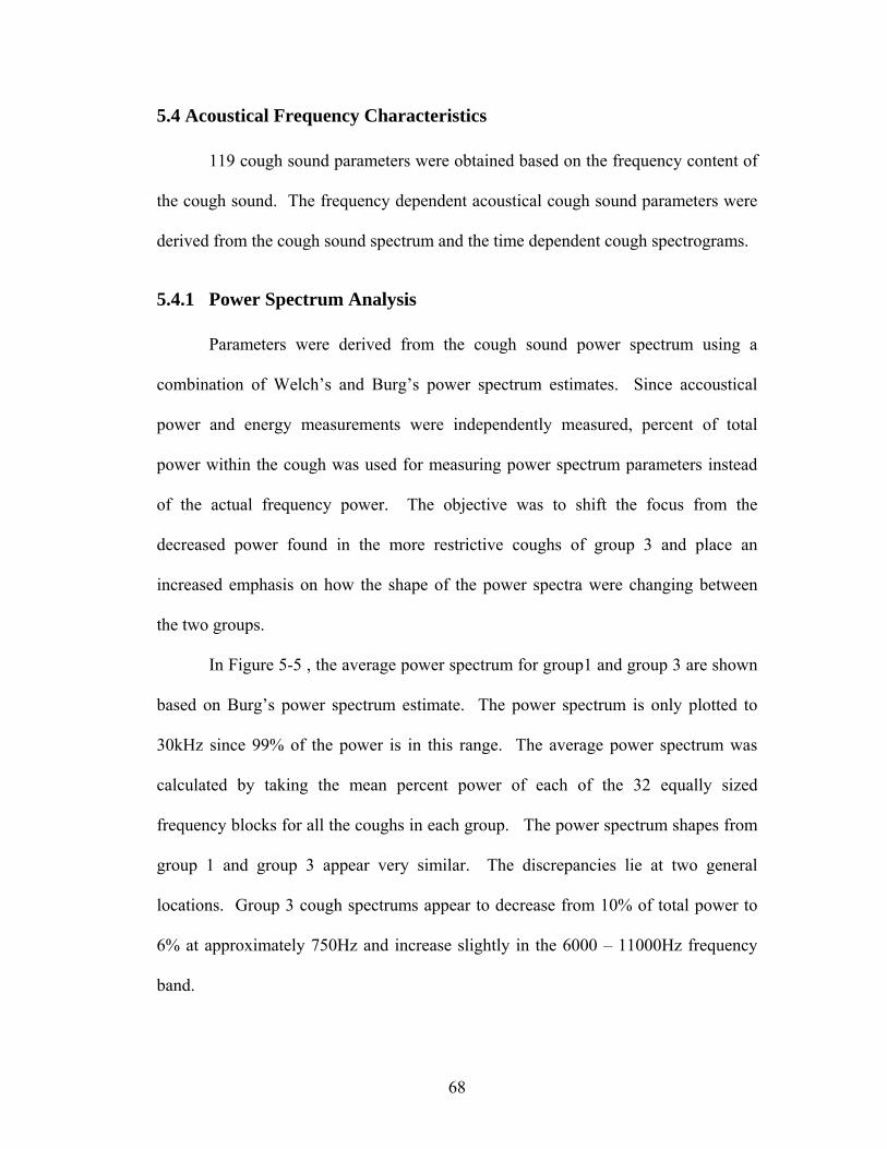
5.4 Acoustical Frequency Characteristics 119 cough sound parameters were obtained based on the frequency content of

the cough sound. The frequency dependent acoustical cough sound parameters were

derived from the cough sound spectrum and the time dependent cough spectrograms.

5.4.1 Power Spectrum Analysis

Parameters were derived from the cough sound power spectrum using a

combination of Welch’s and Burg’s power spectrum estimates. Since accoustical

power and energy measurements were independently measured, percent of total

power within the cough was used for measuring power spectrum parameters instead

of the actual frequency power. The objective was to shift the focus from the

decreased power found in the more restrictive coughs of group 3 and place an

increased emphasis on how the shape of the power spectra were changing between

the two groups.

In Figure 5-5 , the average power spectrum for group1 and group 3 are shown

based on Burg’s power spectrum estimate. The power spectrum is only plotted to

30kHz since 99% of the power is in this range. The average power spectrum was

calculated by taking the mean percent power of each of the 32 equally sized

frequency blocks for all the coughs in each group. The power spectrum shapes from

group 1 and group 3 appear very similar. The discrepancies lie at two general

locations. Group 3 cough spectrums appear to decrease from 10% of total power to

6% at approximately 750Hz and increase slightly in the 6000 – 11000Hz frequency

band.

68

Average Percent Power Spectrums

-5

0

5

10

15

20

25

30

35

40

45

0 3000 6000 9000 12000 15000 18000 21000 24000 27000 30000

Frequency (Hz)

Perc

ent P

ower

Group1 Group 3

Figure 5-5 Burg’s Average Percent Power Spectrum Figure 5-5 suggests that the dominant frequencies are near 2200Hz for both

groups. Dominant frequencies were recorded based on the frequency with the most

power based on Welch’s and Burg’s power spectrum estimates. The dominant

frequencies are shown for each power spectrum in Figures 5-6 and 5-7.

Dominant Frequency vs. Group using Welch's Method

2900

3100

3300

3500

3700

3900

1 3

Group

Freq

uenc

y (H

z)

Figure 5-6 Dominant Frequency using Welch’s Power Spectrum

69

Dominant Frequency vs. Group using Burg's Method

2900

3100

3300

3500

3700

1 3

Group

Freq

uenc

y (H

z)

Figure 5-7 Dominant Frequency using Burg’s Power Spectum

The dominant frequencies appear to be slightly higher than indicated by the

average power spectrum in Figure 5-5. This can be attributed to the fact that 12.5%

of coughs in group 1 and 17% of coughs in group 3 contained dominant frequencies

greater than 3kHz. Upon examining the power spectrums and spectrograms in greater

detail, the coughs having dominant frequencies greater than 3kHz had a pronounced

wheeze in frequency bands greater than 3kHz causing the shift in dominant

frequencies.

Another common acoustical analysis technique is an octave analyzer. Since

an octave analyzer uses a nonlinear frequency scale, the information derived from the

power spectrum could be more diversified. The octave analyzer used for analyzing

the cough sound is defined by Table 5-2.

Table 5-2 Octave Frequency Breakdown

Octave 1 2 3 4 5 6 7 Frequency (kHz) 0.5 – 1 1 – 2 2 – 4 4 – 8 8 – 16 16 – 32 32 - 49 14 cough parameters were obtained from the following octave analysis using Welch’s

and Burg’s power spectrum estimates. The results are shown in Figures 5-8 and 5-9.

70

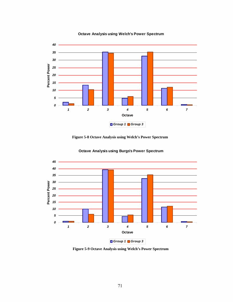
Octave Analysis using Welch's Power Spectrum

0

5

10

15

20

25

30

35

40

1 2 3 4 5 6 7

Octave

Perc

ent P

ower

Group 1 Group 3

Figure 5-8 Octave Analysis using Welch’s Power Spectrum

Octave Analysis using Burgs's Power Spectrum

0

5

10

15

20

25

30

35

40

45

1 2 3 4 5 6 7

Octave

Perc

ent P

ower

Group 1 Group 3

Figure 5-9 Octave Analysis using Welch’s Power Spectrum

71

The results of the octave analysis are similar for both power spectrum

estimation techniques. The percent powers in the first three octaves and the last

octave are slightly lower in group 3. The power from these octaves appear to be

transferred to octaves four through six. This indicates that coughs occurring during

high airway resistances exhibit a higher percentage of power in the 4 – 32kHz

frequency range. This does not suggest that coughs occurring at higher airway

resistances have more power at higher frequencies. To illustrate this point consider

the power spectra and octave analysis of a cough selected from group 1 and a cough

selected and group 3. See Figures 5-10 and 5-11.

Figure 5-10 Power Spectrum Comparison for a Cough from Group 1 and a Cough from Group 3

72

Octave Analysis using Welch's Power Spectrum

0

10

20

30

40

50

60

1 2 3 4 5 6 7

Octave

Perc

ent P

ower

Selected Group 1 Cough Selected Group 3 Cough

Figure 5-11 Octave Comparison for a Cough from Group 1 and a Cough from Group 3

Although the percent power in octaves four through six are higher for the

cough from group 3, the power spectrum indicates that the total power is less in all

octaves. The higher octaves contain a higher percentage of power in the cough from

group 3 due to the decreased power in the lower octaves, particularly octaves two and

three.

5.4.2 Spectrogram Estimate

The parameters derived from the cough sound spectrograms were used to

quantify the frequency changes at different times within the cough. Dominant

frequency, average frequency, and midpoint power in frequency bands represent 70

parameters obtained from the spectrograms. Since the cough lengths varied greatly

within each group, parameters were derived based on time relative to the duration of

the cough. In the dominant frequency plot, the cough was divided into ten time

frames and the frequency containing the maximum power was recorded. The average

73

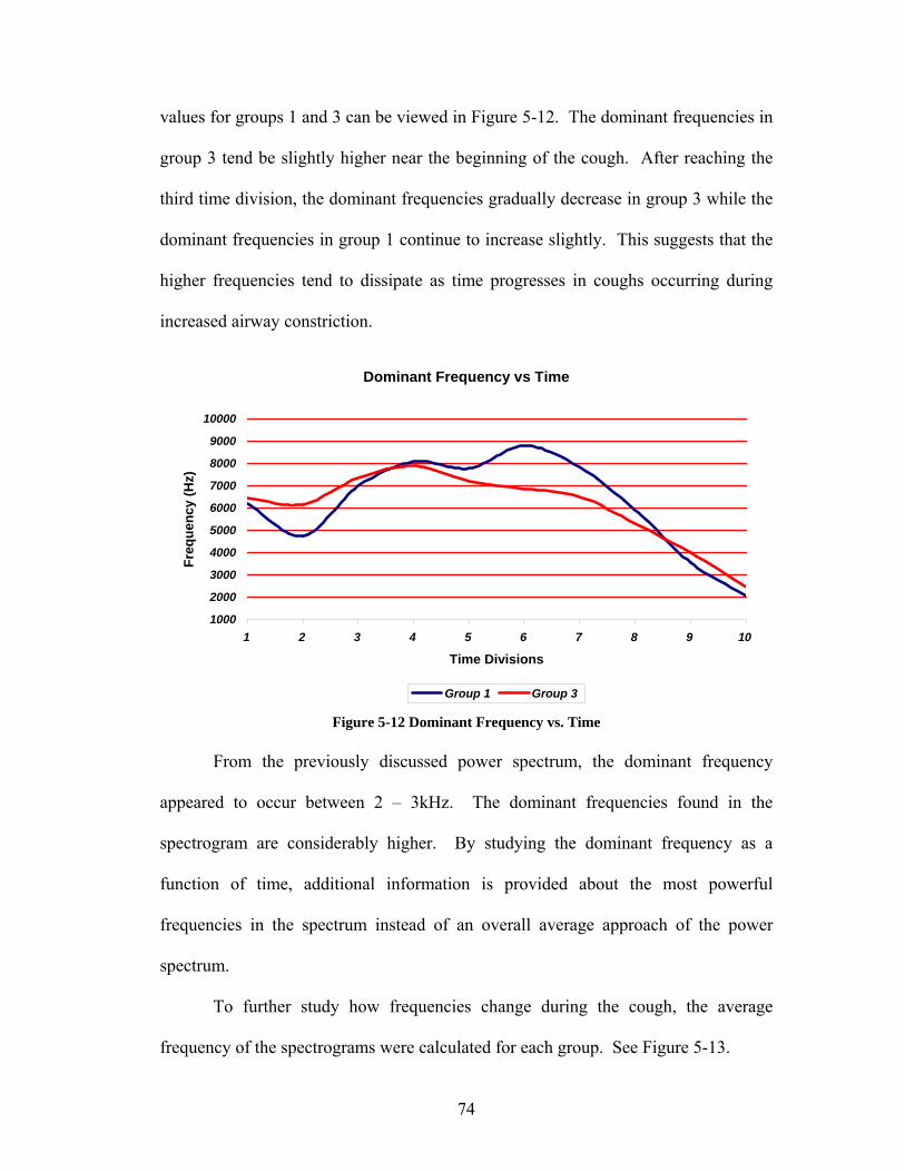
values for groups 1 and 3 can be viewed in Figure 5-12. The dominant frequencies in

group 3 tend be slightly higher near the beginning of the cough. After reaching the

third time division, the dominant frequencies gradually decrease in group 3 while the

dominant frequencies in group 1 continue to increase slightly. This suggests that the

higher frequencies tend to dissipate as time progresses in coughs occurring during

increased airway constriction.

Dominant Frequency vs Time

1000

2000

3000

4000

5000

6000

7000

8000

9000

10000

1 2 3 4 5 6 7 8 9 10

Time Divisions

Freq

uenc

y (H

z)

Group 1 Group 3

Figure 5-12 Dominant Frequency vs. Time

From the previously discussed power spectrum, the dominant frequency

appeared to occur between 2 – 3kHz. The dominant frequencies found in the

spectrogram are considerably higher. By studying the dominant frequency as a

function of time, additional information is provided about the most powerful

frequencies in the spectrum instead of an overall average approach of the power

spectrum.

To further study how frequencies change during the cough, the average

frequency of the spectrograms were calculated for each group. See Figure 5-13.

74

Spectrogram Average Frequency Vector

1050011000115001200012500130001350014000145001500015500

0 5 10 15 20 25 30 35

Time Divisions

Freq

uenc

y (H

z)

Group1 Group 3

Figure 5-13 Average Frequency Comparison vs. Time The average frequency vector shows how the shape of the spectrogram is

changing by splitting the spectrogram horizontally based on the power weighted

frequency averages. Interestingly, the shapes of the spectrograms from both groups

are quite similar. The differences lie in the overall pitch of the coughs. During the

start of the coughs in group 3, the average frequency is slightly higher and drops

immediately after the initial cough sound. After the initial drop, the average

frequencies are lower for coughs in group 3 indicating the power is more compressed

into the lower frequencies of the group 3 coughs. To illustrate this point further,

examine spectrograms in Figures 5-14 and 5-15. After 0.02 seconds the power in the

selected group 3 cough is primarily limited to frequencies below 20kHz while

frequencies up to 30kHz are present throughout the majority of the cough selected

from group 1.

75

Figure 5-14 Group 1 Cough Spectrogram

Figure 5-15 Group 3 Cough Spectrogram

76

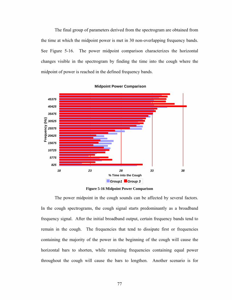
The final group of parameters derived from the spectrogram are obtained from

the time at which the midpoint power is met in 30 non-overlapping frequency bands.

See Figure 5-16. The power midpoint comparison characterizes the horizontal

changes visible in the spectrogram by finding the time into the cough where the

midpoint of power is reached in the defined frequency bands.

Midpoint Power Comparison

18 23 28 33 38

825

5775

10725

15675

20625

25575

30525

35475

40425

45375

Freq

uenc

y (H

z)

% Time into the Cough

Group1 Group 3

Figure 5-16 Midpoint Power Comparison

The power midpoint in the cough sounds can be affected by several factors.

In the cough spectrograms, the cough signal starts predominantly as a broadband

frequency signal. After the initial broadband output, certain frequency bands tend to

remain in the cough. The frequencies that tend to dissipate first or frequencies

containing the majority of the power in the beginning of the cough will cause the

horizontal bars to shorten, while remaining frequencies containing equal power

throughout the cough will cause the bars to lengthen. Another scenario is for

77

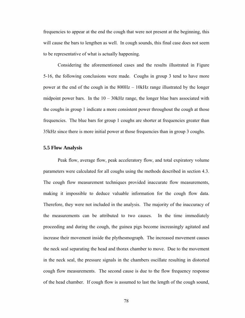
frequencies to appear at the end the cough that were not present at the beginning, this

will cause the bars to lengthen as well. In cough sounds, this final case does not seem

to be representative of what is actually happening.

Considering the aforementioned cases and the results illustrated in Figure

5-16, the following conclusions were made. Coughs in group 3 tend to have more

power at the end of the cough in the 800Hz – 10kHz range illustrated by the longer

midpoint power bars. In the 10 – 30kHz range, the longer blue bars associated with

the coughs in group 1 indicate a more consistent power throughout the cough at those

frequencies. The blue bars for group 1 coughs are shorter at frequencies greater than

35kHz since there is more initial power at those frequencies than in group 3 coughs.

5.5 Flow Analysis

Peak flow, average flow, peak acceleratory flow, and total expiratory volume

parameters were calculated for all coughs using the methods described in section 4.3.

The cough flow measurement techniques provided inaccurate flow measurements,

making it impossible to deduce valuable information for the cough flow data.

Therefore, they were not included in the analysis. The majority of the inaccuracy of

the measurements can be attributed to two causes. In the time immediately

proceeding and during the cough, the guinea pigs become increasingly agitated and

increase their movement inside the plythesmograph. The increased movement causes

the neck seal separating the head and thorax chamber to move. Due to the movement

in the neck seal, the pressure signals in the chambers oscillate resulting in distorted

cough flow measurements. The second cause is due to the flow frequency response

of the head chamber. If cough flow is assumed to last the length of the cough sound,

78

then the duration of expired air exiting the mouth of the guinea pig is very short,

approximately 1/10th of a second. The short duration of increased flow being expired

from the mouth of the guinea pig in conjunction with the capacitance created by the

relatively large volume of the head chamber provided a poor cough flow frequency

response.

5.6 Cough Characteristics versus Airway Resistance From the results of previously described cough sound and flow analysis, 124

cough sound parameters were used in classifying coughs. Cough parameters obtained

from the training dataset were analyzed using principal component analysis (PCA).

The number of principal component vectors to be used in the analysis was based on

the classification accuracy of the neural net. The best results were obtained using the

first 62 principal components. The covariance matrix indicated the selected principal

components accounted for 99.5% of the variability in the dataset. PCA enabled the

cough parameter dimensions to be reduced by half while accounting for over 99% of

the variability in the measurements. To obtain the new cough parameters for training

and test datasets, the original parameters were multiplied by the principal component

vectors.

The new cough parameters from the train dataset were then submitted to the

neural net to appropriately weight the new cough parameters. A neural net was

trained with and without the coughs from group 2. The neural net trained without the

coughs from group 2 provided excellent results for the training set but decreased

accuracy in classifying coughs from groups 1 and 3 in the test set. For this analysis,

79

coughs from group 2 were included in the training to provide the best overall

separation between groups 1 and 3.

Coughs from groups 1, 2, and 3 were trained with target outputs of –1, 0, and

1 respectively. The training results are represented in Figure 5-17 as a cumulative

distribution plot. The cumulative distribution plot tells the probability of having a

cough in any group below a selected neural net output. It also provides a visual index

to how well the neural net separated the coughs.

-1 -0.8 -0.6 -0.4 -0.2 0 0.2 0.4 0.6 0.8 10

0.1

0.2

0.3

0.4

0.5

0.6

0.7

0.8

0.9

1Cumulative Distribution for the Train Dataset

Neuron Output

Prob

abili

ty

Group 1 coughsGroup 2 coughsGroup 3 coughs

Figure 5-17 Cumulative Distribution Plot for Train Dataset

Using the principal component vectors and the neural net weights generated

from the train dataset, the following results were obtained for the test dataset. See

Figure 5-18.

80

-1 -0.8 -0.6 -0.4 -0.2 0 0.2 0.4 0.6 0.8 10

0.1

0.2

0.3

0.4

0.5

0.6

0.7

0.8

0.9

1

Cumulative Distribution for the Test Dataset

Neuron Output

Prob

abili

ty

Group 1 coughsGroup 2 coughsGroup 3 coughs

Figure 5-18 Cumulative Distribution for Test Dataset

The cumulative distributions for the train and test datasets show significant

separation in coughs occurring in groups 1 and 3. The transition group, group 2,

spans the range of the neuron output. This was expected given that group 2

represents coughs occurring between the airway resistance ranges specified by groups

1 and 3.

Since the focus of this analysis is to design a classification system capable of

distinguishing coughs occurring during times of low airway resistance from coughs

occurring during high airway resistances, a Receiver Operating Characteristic (ROC)

curve was created to determine the accuracy and cutoff for separating the two groups.

An ROC analysis provides a more comprehensive evaluation of the neural network

81

output and illustrates the cost/benefit relationship as a result of choosing different

decision making criteria. See Figure 5-19.

0 0.1 0.2 0.3 0.4 0.5 0.6 0.7 0.8 0.9 10

0.2

0.4

0.6

0.8

1

P (False Group 1)

P (T

rue

Gro

up 1

)ROC for Group 1 and Group 3

Figure 5-19 Group 1 and Group 3 ROC Curve for Test Dataset

P(True Group 1) is the probability of accurately classifying a cough into group

1, and P(False Group 1) is the probability of classifying a cough as group 1 when the

cough belongs in group 3. An ROC curve can be described by three parameters. The

first parameter is accuracy or the area under the curve. The area under the curve is

the overall ability of the cough analysis to correctly classify coughs into group 1 and

group 3. The second parameter is sensitivity, which measures the percent of accurate

group 1 classifications. The final parameter, specificity, measures the percent of

accurate group 3 classifications. Sensitivity and specificity are inversely related and

the decision threshold can be adjusted to favor sensitivity or specificity. The

accuracy of the ROC curve is 0.946 with equal sensitivity and specificity at 0.893.

82

Chapter 6 – Conclusions and Future Recommendations

6.1 Conclusions

This thesis has displayed the engineering process involved in this area of

research up to this point; including the primary concept and motivation, through the

equipment selection and calibration, the signal processing of the acquired cough

sounds, to the cough classification algorithm. The goal of designing an exposure

system that can be used to collect acoustical information within a guinea pig cough

and depict changes in the acoustical properties at low and high levels of chemically

induced airway resistance has been accomplished. Flow measurements and analysis

are still unrefined.

A large number of parameters were developed for the acoustical cough

characterization due to the variability in cough length, differences in cough sounds

between guinea pigs, and the lack of initial knowledge as to how the cough sound

would change with respect to airway resistance. Based on the results of the analysis,

the developed cough parameters appear to provide significant information to how the

cough sound changed from low to high levels of chemically induced airway

resistance. Since many cough parameters may reflect similar information about the

cough, principal component analysis provided a way to effectively reduce the

redundancy in the parameters.

The animal cough model shows that changes in the acoustical characteristics

of the guinea pig cough can be used to reflect alterations in pulmonary function.

Accurately characterizing the cough sound and diagnosing guinea pigs with

83

significantly increased airway resistance is the first step in analyzing the effects of

other pulmonary irritants on cough sound.

6.2 Future Recommendations While the present work on this project has provided valuable results, there are

a number of methods considered paramount to the success of future iterations of this

design and process. Numerous other signal processing techniques can be applied to

extract more information from the cough sound and form new cough parameters.

Sound reverberations present in the head chamber need to be addressed from a signal

processing standpoint or through a redesign of the head chamber. From a

comparative perspective, reverberations caused by the head chamber are negligible.

In order to accurately characterize the cough sound, reverberations must be

attenuated.

A more accurate way to measure cough flow is also needed. Reducing the

volume of the head chamber may help with the inadequate flow frequency response,

but animal movement during the cough would also need to be considered. The head

chamber could be modified in a way to restrain head movement during the cough.

Upon addressing the aforementioned issues, additional exposures are needed

to validate the findings supported in this thesis. The use of bronchodilating chemicals

to induce cough would extend the range of airway measurements and further enhance

the study. It would also be interesting to conduct and compare the results from a

similar study based on the coughs from a single animal, providing enough coughs

with varying airway resistances could be gathered.

84

The next phase of research would be to compare cough flow and acoustical

characteristics before and after exposures to common occupational pulmonary

irritants. Changes in guinea pig cough characteristics could then be compared to

known changes found in human cough characteristics. The validity of the animal

cough model could then be examined in more detail.

85

Appendix A – Complete Hardware Specifications

MASS AIRFLOW CONTROLLERS

Use Nebulized Airflow Controller Dilutant Airflow Controller

Part No. GFC1735 G20589C

Flow Range

0 – 5 L/min 0 – 10 L/m

Max Input Pressure

500 psig (34.5 bars) 500 psig (34.5 bars)

Leak Integrity

1 x 10-7 of helium 1 x 10-7 of helium

Setpoint Control

Local or remote Local or remote

Analog out 0-5 Vdc and 4-20 mA 0-5 Vdc and 4-20 mA

Other Specs.

• NIST traceable certification • circuit protection • totalizer option

86

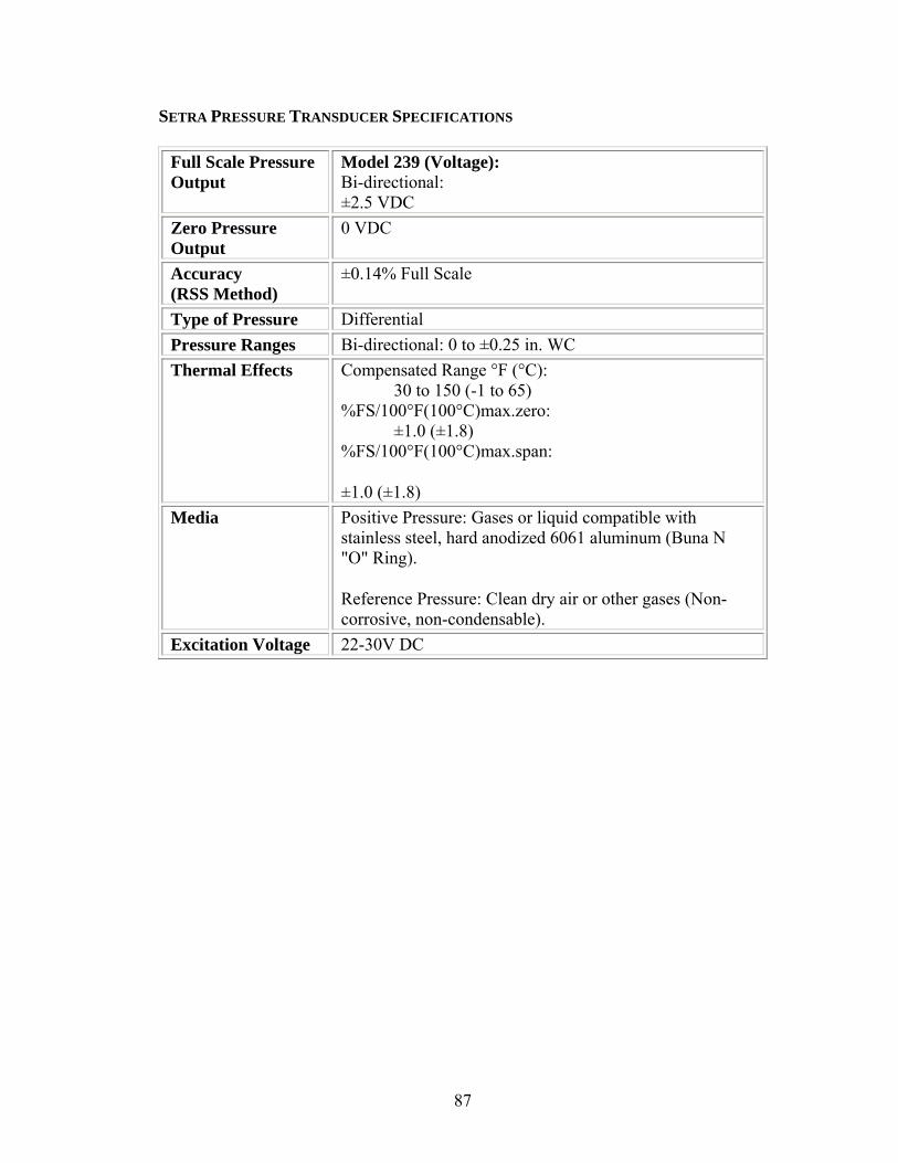
SETRA PRESSURE TRANSDUCER SPECIFICATIONS

Full Scale Pressure Output

Model 239 (Voltage): Bi-directional: ±2.5 VDC

Zero Pressure Output

0 VDC

Accuracy (RSS Method)

±0.14% Full Scale

Type of Pressure Differential Pressure Ranges Bi-directional: 0 to ±0.25 in. WC Thermal Effects Compensated Range °F (°C):

30 to 150 (-1 to 65) %FS/100°F(100°C)max.zero:

±1.0 (±1.8) %FS/100°F(100°C)max.span:

±1.0 (±1.8) Media Positive Pressure: Gases or liquid compatible with

stainless steel, hard anodized 6061 aluminum (Buna N "O" Ring).

Reference Pressure: Clean dry air or other gases (Non-corrosive, non-condensable).

Excitation Voltage 22-30V DC

87

AUDIO SPECIFICATIONS

Microphone

Model Number 2530

Nominal Diameter (inches) 1/4

Directive Characteristics Random incidence & pressure Frequency Response 4 Hz to 80 kHz

mV/Pa 1.3 Nominal Open Circuit Sensitivity

dB rel. 1V/Pa -57.7

Lower Limiting Frequency (Hz) 0.2 to 2 Open Circuit Distortion Limit 3% (dB rel. 20 µPa)

>172

Nominal Cartridge Thermal Noise [dB(A)]

31

Resonant Freq. (kHz) 80 Polarization Voltage (Vdc) 200

Preamplifier

Model PRM910B ICP Preamplifier PRM422 Size 1/4 in Power Dual ± 10 to ± 18 V

Single 20 to 35 V Output Connector 5-pin Switchcraft® Cable 6 ft, Integral cable

88

AUDIO SPECIFICATIONS (CONT.) Power Supply Bandwidth/Response Lower limiting frequency as function of gain setting Gain (dB) -3 dB Point (Hz) -2 dB Point (Hz) 0 0.2 1.0 10 0.4 2.0 20 1.6 81.0 Upper limiting frequency as function of output voltage (flat output) Output Voltage RMS -3 dB Point (Hz) 10.0 50K 5.0 100K 2.0 250K 1.0 500K 0.5 1M Signal Input (each channel) Gain 0 to 40 dB in 10 dB steps

Attenuation 0 to 30 dB in 10 dB steps plus 22-turn vernier attenuator providing 0 to 10.4 dB continuous range.

Bias Voltage 0, 28, 100, 200 Vdc, ±0.5% stability Input Impedance 20 kOhms @ 0 dB attenuation 70 kOhms @ 10 dB attenduation

Crosstalk 80 dB to 20 kHz 60 dB to 200 kHz

Connector Type

Switchcraft miniature XLR 5-pin (part no. TB4M) Cable requires TA5F connector

Overload 10 V rms Signal Output (each channel) Impedance 50 Ohms Output Noise (dB reference 1 µV)

Gain (dB) Flat (dB) (1 Hz - 20 kKz) A-weight (dB) C-Weight (dB)

0 8.3 (2.6 µV) 0 (1 µV) 3.4 (1.5 µV) 40 35.3 (58.2 µV) 32.2 (40.7 µV) 30.9 (35.2 µV)

89

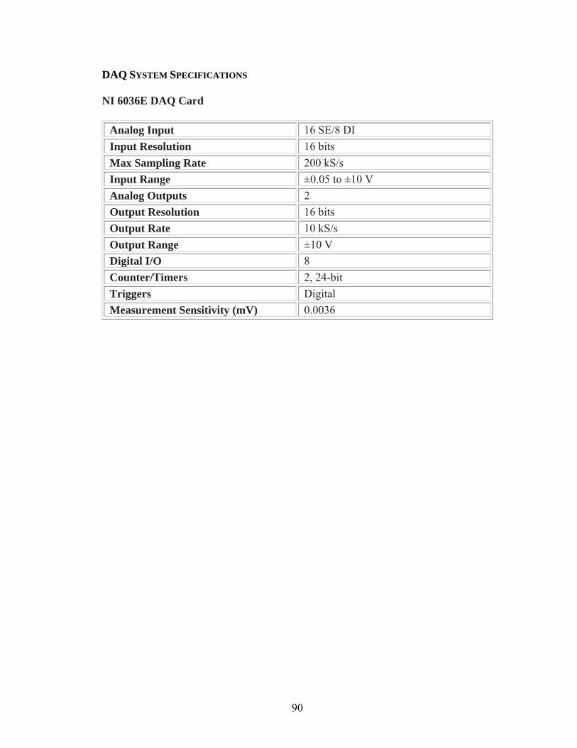
DAQ SYSTEM SPECIFICATIONS NI 6036E DAQ Card

Analog Input 16 SE/8 DI Input Resolution 16 bits Max Sampling Rate 200 kS/s Input Range ±0.05 to ±10 V Analog Outputs 2 Output Resolution 16 bits Output Rate 10 kS/s Output Range ±10 V Digital I/O 8 Counter/Timers 2, 24-bit Triggers Digital Measurement Sensitivity (mV) 0.0036

90

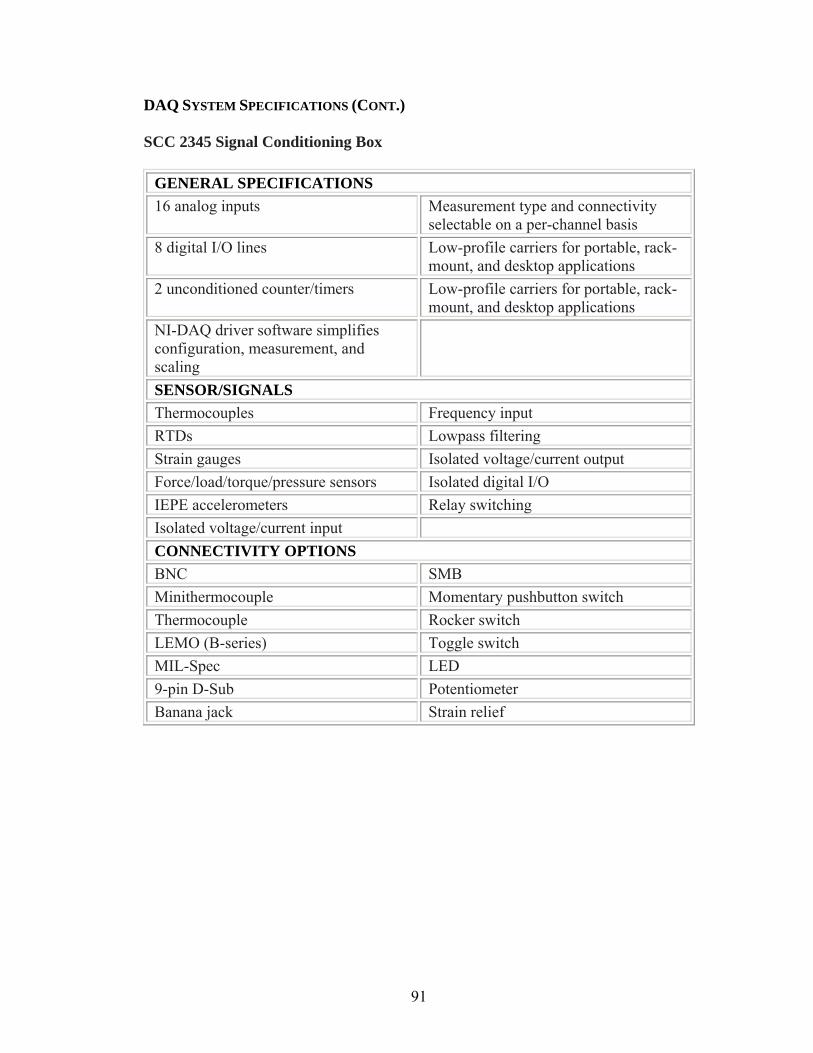
DAQ SYSTEM SPECIFICATIONS (CONT.) SCC 2345 Signal Conditioning Box

GENERAL SPECIFICATIONS 16 analog inputs Measurement type and connectivity

selectable on a per-channel basis 8 digital I/O lines Low-profile carriers for portable, rack-

mount, and desktop applications 2 unconditioned counter/timers Low-profile carriers for portable, rack-

mount, and desktop applications NI-DAQ driver software simplifies configuration, measurement, and scaling

SENSOR/SIGNALS Thermocouples Frequency input RTDs Lowpass filtering Strain gauges Isolated voltage/current output Force/load/torque/pressure sensors Isolated digital I/O IEPE accelerometers Relay switching Isolated voltage/current input CONNECTIVITY OPTIONS BNC SMB Minithermocouple Momentary pushbutton switch Thermocouple Rocker switch LEMO (B-series) Toggle switch MIL-Spec LED 9-pin D-Sub Potentiometer Banana jack Strain relief

91

NI PCI-4451 DAQ Card

GENERAL SPECIFICATIONS Analog Input 2 Input Resolution 16 bits Max Sampling Rate 204.8 kS/s Input Range ±10mV to ±42.4 V Analog Outputs 2 Output Resolution 16 bits Output Rate 51.2 kS/s Output Range ±10mV to 10V Digital I/O 8 Triggering Analog/Digital DYNAMIC CHARACTERISTICS Alias-free Bandwidth DC to 0.464 fs Alias Rejection 80 dB, 0.536 ƒs < ƒin < 63.464 ƒs Spurious-free Dynamic Range 90 dB THD -80 dB; -90 dB for ƒin < 20 kHz IMD -100 dB (CCIF 14 kHz + 15 kHz) Crosstalk (Channel Seperation) -100 dB, DC to 100 kHz

92

Appendix B – Airway Resistance Circuit Analysis

Let PT = u

PH = y

KCL CGRAW iiD += (1)

dtduC

Ru

dtdVC

Rui

RuD T

ST

CTT

STCT

ST

+=+=+= (2)

SH

HSH

CHHRSHCHRAW R

ydtdyC

Ry

dtdVCiii +=+=+= (3)

dt

dVCi CGGCG = (4)

yRiyVV AWRAWRAWCG +=+= (5)

combining equations 3 and 5

yR

ydtdyCRV

SHHAWCG +⎟⎟

⎠

⎞⎜⎜⎝

⎛+= (6)

combining equations 4 and 6

⎟⎟⎠

⎞⎜⎜⎝

⎛+⎟⎟⎠

⎞⎜⎜⎝

⎛+= y

Ry

dtdyCR

dtdCi

SHHAWGCG (7)

substituting equations 2, 3, and 7 into equation 1 yields

93

⎟⎟⎠

⎞⎜⎜⎝

⎛+⎟⎟⎠

⎞⎜⎜⎝

⎛++++=+ y

Ry

dtdyCR

dtdCi

Ry

dtdyC

dtduC

Ru

SHHAWGCG

SHHT

ST

(8)

dtdyC

dtdy

RCR

dtydCCRi

Ry

dtdyC

dtduC

Ru

GSH

GAWHGAWCG

SHHT

ST

+++++=+ 2

2

(9)

Laplace of equation 9

YsCYsR

CRYsCCRiRYYsCUsC

RU

GSH

GAWHGAWCG

SHHT

ST

+++++=+ 2 (10)

YsCsR

CRsCCRiR

sCsCR

U GSH

GAWHGAWCG

SHHT

ST⎟⎟⎠

⎞⎜⎜⎝

⎛+++++=⎟⎟

⎠

⎞⎜⎜⎝

⎛+ 211 (11)

YsCR

sCsCRiR

sCsCR

U GSH

HGAWCGSH

HTST

⎥⎦

⎤⎢⎣

⎡+⎟⎟

⎠

⎞⎜⎜⎝

⎛+++⎟⎟

⎠

⎞⎜⎜⎝

⎛+=⎟⎟

⎠

⎞⎜⎜⎝

⎛+

111 (12)

YsCR

sCRsCRiR

sCRR

sCRU GSH

HSHGAWCG

SH

HSH

ST

TST ⎥⎦

⎤⎢⎣

⎡+⎟⎟

⎠

⎞⎜⎜⎝

⎛ +++⎟⎟

⎠

⎞⎜⎜⎝

⎛ +=⎟⎟

⎠

⎞⎜⎜⎝

⎛ + 111 (13)

TTST

ST ZsCR

R=

+1 (14)

HHSH

SH ZsCR

R=

+1 (15)

The circuit can then be simplified and rewritten as

94

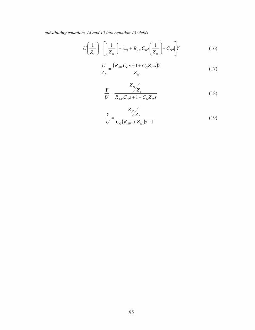
substituting equations 14 and 15 into equation 13 yields

YsCZ

sCRiZZ

U GH

GAWCGHT

⎥⎦

⎤⎢⎣

⎡+⎟⎟

⎠

⎞⎜⎜⎝

⎛++⎟⎟

⎠

⎞⎜⎜⎝

⎛=⎟⎟

⎠

⎞⎜⎜⎝

⎛ 111 (16)

( )H

HGGAW

T ZYsZCsCR

ZU ++

=1 (17)

sZCsCR

ZZ

UY

HGGAW

T

H

++=

1 (18)

( ) 1++=

sZRCZ

Z

UY

HAWG

T

H

(19)

95

References

1. Korpas J., and Tomori Z. Cough and other Respiratory reflexes. In: Herzog E

S ed. Progress in Respiration Research. Basel: Karger, 1979: 15-179 2. Fuller RW. Cough. In: Respiratory Medicine, 2nd edition, Ed. Brewis RAL,

Corrin B, Geddes DM, Gibson GJ. London: WB Saunders Company Limited, 1995: 238-242

3. Goldsmith WT, Friend KA, McKinney WG, Reynolds JS, Frazer DG, Smith

J. An improved system for measuring breath and cough sounds [Abstract]. In: Proceedings of the 24th International Lung Sounds Conference. Marburg, Germany: International Lung Sound Associations, 1999: 35

4. Reynolds JS, McKinney WG, Goldsmith WT, Frazer DG. A system for

reconstruction of cough sounds and components of cough sounds [Abstract]. In: Proceedings of the 24th International Lung Sounds Conference. 1999: 37

5. Friend KA, Goldsmith WT, Reynolds JS, Frazer DG. Acoustic tube

reconstruction for the characterization of cough sounds. In: Proceedings of the First Joint BMES/EMBS Conference. 1999: 1017

6. Goldsmith WT, Reynolds JS, McKinney WG, Friend KA, Shahan D, Frazer

DG. A system for recording high fidelity cough sound measurements. In: He B, Yana K, Cerutti S, eds,. Proceedings of the 3rd International Workshop on Biosignal Interpretationl. 1999: 178-181

7. Goldsmith WT, Reynolds JS, McKinney WG, Friend KA, Stolarik BM,

Frazer DG. Mouth flow estimation during cough sound measurements [Abstract]. In: Proceedings of the 19th Southern Biomedical Engineering Conference. 2000: 78

8. Rosenberry K, Goldsmith WT, Reynolds JS, McKinney W, Frazer DG.

Gender differences in voluntary cough sound spectra demonstrated by an inverse power law analysis [Abstract]. In: Proceedings of the Second Joint BMES/EMBS Conference. IEEE. 2002: 139

9. Colerridge JCG, Coleridge HM. Afferent vagal c-fibre innervation of the

lungs and airways and its functional significance. Rev Physiol Biochem Pharmacol. 1984; 99: 1-110

10. Collier JG, Fuller RW. Capsaicin induced inhalation in man and the effect of

disodium cromoglycate. Br J Pharmacol 1984; 81: 113-117 11. Shannon R, Baekey DM, Morris KF, Lindsey BG. Brainstem respiratory

networks and cough. Pulm Pharmacol 1996; 9: 343-347

96

12. Jordan D. Central nervous mechanisms in cough. Pulm Pharmacol 1972;

22: 634-643 13. van Lunteren E. Daniel R, Deal EC Jr, Haxhiu MA. Role of costal and crural

diaphragm and parasternal intercostals during coughing in cats. J Appl Physiol 1989; 66: 135-141

14. Wallois F, Macron JM. Nasal air puff stimulations and laryngeal, thoracic

and abdominal muscle activities. Respir Physiol 1994; 97: 47-62 15. van Lunteren E, Haxhiu MA, Cherniack NS, Arnold JS. Role of triangularis

sterni during coughing and sneezing in dogs. J Appl Physiol 1988; 65: 2440-2445.

16. Frazer D, Stolarik B, McKinney W, Stone S, Afshari A, Goldsmith T, Barkley

J, Reynolds J, Weber K. Differences in airflow patterns during voluntary coughs that result from obstructive lung disease [Abstract]. Biomed Eng: Recent Developments 2002: 317-318

17. Friend KA, Goldsmith WT, McKinney WG, Watkins SA, Frazer DG,

Salahuddin N, Petsonk EL, Abrons H. Wavelet analysis for the detection of wheeze in cough sounds. In: He B, Yana K, Cerutti S, eds. Proceedings of the 3rd International Workshop on Biosignal Interpretationl. 1999: 326-329

18. Rabiner, L.R. and Schafer R.W. Digital Processing of Speech Signals.

Prentice Hall Inc., Upper Saddle River, New Jersey 1978 19. Van Hirtum, A, Berckmans D, Demuynck K, Van Compernolle D.

Autoregressive acoustical modeling of free field cough sound. IEEE 09/02: 493-495

20. Castranova V, Frazer DG, Manly LK, Dey RD. Pulmonary Alterations

associated with inhalation of occupational and environmental irritants. International Immunopharmacology 2 2002: 163-172

21. Laude EA, Higgins KS, Morice AH. A comparative Study of the Effects of

Citric Acid, Capsaicin and Resiniferatoxin on the Cough Challenge in Guniea pig and Man. Pulmonary Pharmacology. 1993; 6, 171-175

22. Tartar M, Pecova R, Karcolova D. Sensitivity of cough reflex in awake

guine-pigs, rats, and rabbits. Bratisl. Lek. Listy. 1997; 10: 539-543 23. Tartar, Kacolova D, Pecova R, Brozmanova M. The Role of partial laryngeal

denervation on the cough reflex in awake guinea-pigs, rats and rabbits. Pulmonary Pharmacology. 1996; 9: 371-372

97

24. Forsberg K, Karlsson JA, Theodorsson E, Lundberg JM, Persson CGA.

Cough and bronchoconstriction mediated by capsaicin-sensitive sensory neurons in the guinea-pig. Pulmonary Pharmacology. 1988; 1: 33-39

25. Sheppard D, Rizk NW, Boushey HA, Bethel RA. Mechanism of cough and

bronchoconstriction induced by distilled water aerosol. Am Rev Respir Dis. 1983; 127: 691-694

26. Clay TP, Thompson MA. Irritant induced cough as a model of

intrapulmonary airway reactivity. Lung 1985; 163: 183-191 27. Allott CP, Evans DP, Marshall PW. A model of irritant-induced

bronchoconstriction in the spontaneously breathing guinea-pig. Br J Pharmacol 1980; 71: 165-168

28. Braman SS, Corrao WM. Chronic cough. Prim Care 1985; 12: 217-25 29. Corrao WM. Chronic cough: an approach to management. Compr Ther

1986;12:14-19 30 Alarie Y, Nielsen GD, Schaper MM. Animal bioassays for evaluation of

indorr air quality. In: Spengler JD, Samet JM, McCarthy JF, editors. Indoor air quality handbook. New York: McGraw-Hill; 2001 p. 23.1-23.49

31 Finger TE, Jeor VLS, Kinnamon JC, Silver WL. Ultrastructure of substance

P- and CGRP-immunoreactive nerve fibers in the nasal epithelium of rodents. J Comp Neurol 1990; 294:293-305.

32 Grunditz T, Uddman R, Sundler F. Origin and peptide content of nerve fibers

in the nasal mucosa of rats. Anat Embryol 1994; 189: 327-337 33 Karlsson JA, Choudry NB, Zackrisson C, Fuller RW. A comparison of the

effect of inhaled diurectics on airway reflexes in humans and guinea pigs. Journal of Applied Physiology 1992; 72: 434-438

34 Bergen DR, Sampson SR. Characterization of intrapulmonary, rapidly

adapting receptors of guinea pigs. Respiratory Physiology 1982; 47: 83-95 35 Sommer B, Montano LM, Chavez J, Gustin P, Vargas MH. Guinea pig lung

resistance shows circadian rhythmicity not influenced by ozone. Respiration Physiology. 1998; 113: 223-229

36 Randall BR. Frequency Analysis. Denmark: K. Larsen and Son; 1987: 19-49 37 Beranek BL. Acoustics. New York: McGraw-Hill Book Co; 1954: 333-334

98

38 Proakis JG, Dimitrix MG. Digital Signal Processing. New Jersey: Prentice Hall; 1996: 49, 400-403, 917, 925-929

39 Agrawal KP. Specific airway conductance in guinea pigs: normal values and

histamine induced fall. Respiratory Phsyiology. 1981; 43: 23-30 40 Porges G. Applied Acoustics. New York: John Wiley and Sons; 1997: 17-18 41 Pennock BE, Cox CP, Rogers RM, Cain WA, and Wells JH. A non-invasive

technique for measurement of changes in specific airway resistance. Journal of Applied Phsyiology. 1979; 46:399

42 Shlens, Jon. A Tutorial on Principal Component Analysis. 2003. Salk Institute

for Biological Studies. 25 March 2003 <http://www.snl.salk.edu/~shlens/pub/notes/pca.pdf>

99