Embed Size (px)
Citation preview

Acoustical response of shear layers
Citation for published version (APA):Kooijman, G. (2007). Acoustical response of shear layers. Technische Universiteit Eindhoven.https://doi.org/10.6100/IR621958
DOI:10.6100/IR621958
Document status and date:Published: 01/01/2007
Document Version:Publisher’s PDF, also known as Version of Record (includes final page, issue and volume numbers)
Please check the document version of this publication:
• A submitted manuscript is the version of the article upon submission and before peer-review. There can beimportant differences between the submitted version and the official published version of record. Peopleinterested in the research are advised to contact the author for the final version of the publication, or visit theDOI to the publisher's website.• The final author version and the galley proof are versions of the publication after peer review.• The final published version features the final layout of the paper including the volume, issue and pagenumbers.Link to publication
General rightsCopyright and moral rights for the publications made accessible in the public portal are retained by the authors and/or other copyright ownersand it is a condition of accessing publications that users recognise and abide by the legal requirements associated with these rights.
• Users may download and print one copy of any publication from the public portal for the purpose of private study or research. • You may not further distribute the material or use it for any profit-making activity or commercial gain • You may freely distribute the URL identifying the publication in the public portal.
If the publication is distributed under the terms of Article 25fa of the Dutch Copyright Act, indicated by the “Taverne” license above, pleasefollow below link for the End User Agreement:www.tue.nl/taverne
Take down policyIf you believe that this document breaches copyright please contact us at:[email protected] details and we will investigate your claim.
Download date: 08. Feb. 2022
Acoustical Response of Shear Layers
by
Gerben Kooijman

Copyright c©2007 G. KooijmanOmslagontwerp/Cover design: Paul Verspaget & Carin Bruinink Grafische vormgev-ingDruk/Printed by: Universiteitsdrukkerij Technische Universiteit Eindhoven
CIP-DATA LIBRARY TECHNISCHE UNIVERSITEIT EINDHOVEN
Kooijman, Gerben
Acoustical Response of Shear Layers / by Gerben Kooijman. -Eindhoven: Technische Universiteit Eindhoven, 2007. - ProefschriftISBN-10: 90-386-2182-5ISBN-13: 978-90-386-2182-1NUR 924Trefwoorden: aero-akoestiek / geluidsleer / geluidsinteractie / stromingsleerSubject headings: aeroacoustics / shear layers / acoustic impedance / multimodalanalysis

Acoustical Response of Shear Layers
PROEFSCHRIFT
ter verkrijging van de graad van doctor aan deTechnische Universiteit Eindhoven op gezag vande Rector Magnificus, prof.dr.ir. C.J. van Duijn,voor een commissie aangewezen door het Collegevoor Promoties in het openbaar te verdedigen op
woensdag 31 januari 2007 om 16.00 uur
door
Gerben Kooijman
geboren te ’s-Hertogenbosch

Dit proefschrift is goedgekeurd door de promotoren:
prof.dr.ir. M.E.H. van Dongenenprof.dr.ir. A. Hirschberg
Copromotor:dr. Y. Auregan
This research was financially supported by the Dutch Technology Foundation STW,grant ESF.5645

De ultieme droom is promoveren
Gert Kruys, trainer FC Den BoschStadsblad ’s-Hertogenbosch, 20 augustus 2003
aan mijn ouders,
aan Lisa


Contents
1 Introduction 11.1 Aeroacoustics . . . . . . . . . . . . . . . . . . . . . . . . . . . . . . . . 11.2 Technological applications . . . . . . . . . . . . . . . . . . . . . . . . . 21.3 Thesis outline . . . . . . . . . . . . . . . . . . . . . . . . . . . . . . . . 2
2 Modal analysis 52.1 Introduction . . . . . . . . . . . . . . . . . . . . . . . . . . . . . . . . . 52.2 Duct modes for non uniform mean flow . . . . . . . . . . . . . . . . . 62.3 Duct modes for partly non-uniform flow . . . . . . . . . . . . . . . . . 102.4 Duct modes for (partly) uniform mean flow . . . . . . . . . . . . . . . 112.5 Duct modes for partly non-uniform flow with velocity jump . . . . . . 142.6 Classification of the modes . . . . . . . . . . . . . . . . . . . . . . . . . 152.7 Comparison with analytical solutions . . . . . . . . . . . . . . . . . . . 21
2.7.1 Acoustic modes . . . . . . . . . . . . . . . . . . . . . . . . . . . 212.7.2 Unstable hydrodynamic modes . . . . . . . . . . . . . . . . . . 272.7.3 Neutral hydrodynamic modes . . . . . . . . . . . . . . . . . . . 35
2.8 Conclusion . . . . . . . . . . . . . . . . . . . . . . . . . . . . . . . . . 39
3 Area expansion in a duct: modal analysis 413.1 Introduction . . . . . . . . . . . . . . . . . . . . . . . . . . . . . . . . . 413.2 Matching modes . . . . . . . . . . . . . . . . . . . . . . . . . . . . . . 44
3.2.1 Without Kutta condition . . . . . . . . . . . . . . . . . . . . . 443.2.2 With Kutta condition . . . . . . . . . . . . . . . . . . . . . . . 463.2.3 Further thoughts about the Kutta condition . . . . . . . . . . . 48
3.3 Influence of flow configuration . . . . . . . . . . . . . . . . . . . . . . . 503.3.1 Flow profile and Kutta condition . . . . . . . . . . . . . . . . . 503.3.2 Area expansion ratio . . . . . . . . . . . . . . . . . . . . . . . . 52
3.4 Cartesian and cylindrical geometry . . . . . . . . . . . . . . . . . . . . 673.4.1 Scaling of the Helmholtz number . . . . . . . . . . . . . . . . . 673.4.2 Comparison rectangular and cylindrical calculations . . . . . . 69

VIII CONTENTS
3.4.3 Influence of ratio of duct radii . . . . . . . . . . . . . . . . . . . 703.5 Comparison with an alternative model and experimental data . . . . . 723.6 Conclusion . . . . . . . . . . . . . . . . . . . . . . . . . . . . . . . . . 82
4 Effect of grazing flow on orifice impedance: experiments 854.1 Introduction . . . . . . . . . . . . . . . . . . . . . . . . . . . . . . . . . 854.2 Quantities for the acoustical behaviour of an orifice . . . . . . . . . . . 854.3 Previous experimental studies . . . . . . . . . . . . . . . . . . . . . . . 884.4 Impedance tube experiment . . . . . . . . . . . . . . . . . . . . . . . . 92
4.4.1 Setup . . . . . . . . . . . . . . . . . . . . . . . . . . . . . . . . 924.4.2 Impedance measurement . . . . . . . . . . . . . . . . . . . . . . 934.4.3 Accuracy . . . . . . . . . . . . . . . . . . . . . . . . . . . . . . 95
4.5 Orifice geometries . . . . . . . . . . . . . . . . . . . . . . . . . . . . . . 954.6 Mean flow properties . . . . . . . . . . . . . . . . . . . . . . . . . . . . 96
4.6.1 Boundary layer characterization . . . . . . . . . . . . . . . . . 964.6.2 Shear layer profiles . . . . . . . . . . . . . . . . . . . . . . . . . 100
4.7 Results . . . . . . . . . . . . . . . . . . . . . . . . . . . . . . . . . . . . 1074.7.1 Impedance without mean flow . . . . . . . . . . . . . . . . . . . 1074.7.2 Impedance with grazing mean flow . . . . . . . . . . . . . . . . 1094.7.3 Linearity . . . . . . . . . . . . . . . . . . . . . . . . . . . . . . 1114.7.4 Non-dimensional scaled resistance and reactance . . . . . . . . 1124.7.5 Effective Strouhal number . . . . . . . . . . . . . . . . . . . . . 1164.7.6 Influence of edge geometry . . . . . . . . . . . . . . . . . . . . 126
4.8 Conclusion . . . . . . . . . . . . . . . . . . . . . . . . . . . . . . . . . 128
5 Grazing flow over an orifice: modal analysis 1295.1 Introduction . . . . . . . . . . . . . . . . . . . . . . . . . . . . . . . . . 1295.2 Mode matching . . . . . . . . . . . . . . . . . . . . . . . . . . . . . . . 1305.3 Calculation of the impedance . . . . . . . . . . . . . . . . . . . . . . . 1335.4 No mean flow . . . . . . . . . . . . . . . . . . . . . . . . . . . . . . . . 135
5.4.1 Convergence . . . . . . . . . . . . . . . . . . . . . . . . . . . . 1355.4.2 Comparison with potential theory . . . . . . . . . . . . . . . . 138
5.5 Uniform flow . . . . . . . . . . . . . . . . . . . . . . . . . . . . . . . . 1405.5.1 Convergence . . . . . . . . . . . . . . . . . . . . . . . . . . . . 1415.5.2 Behaviour at the edges of the orifice . . . . . . . . . . . . . . . 1415.5.3 Influence of impedance definition . . . . . . . . . . . . . . . . . 1445.5.4 Incompressible limit . . . . . . . . . . . . . . . . . . . . . . . . 1465.5.5 Influence of ratio of duct height and orifice width . . . . . . . . 148
5.6 Non-uniform flow . . . . . . . . . . . . . . . . . . . . . . . . . . . . . . 1515.6.1 Influence of impedance definition . . . . . . . . . . . . . . . . . 1515.6.2 Convergence . . . . . . . . . . . . . . . . . . . . . . . . . . . . 1535.6.3 Influence of boundary layer thickness . . . . . . . . . . . . . . . 156

CONTENTS IX
5.7 Conclusion . . . . . . . . . . . . . . . . . . . . . . . . . . . . . . . . . 158
A Source model for orifice impedance under uniform grazing flow 161
B Hydrodynamic (in)stability of a free shear layer 167B.1 Rayleigh’s equation . . . . . . . . . . . . . . . . . . . . . . . . . . . . . 167B.2 The generalized hyperbolic-tangent shear layer profile . . . . . . . . . 168
C Differential matrices 171
D Continuity conditions mode matching 175
E Modal analysis in 2D cylindrical geometry 177
Bibliography 179
Summary 189
Samenvatting 193
Dankwoord 197
Curriculum vitae 199


Chapter 1
Introduction
1.1 Aeroacoustics
Originally, acoustics was the study of small pressure perturbation waves in air, whichcan be detected by the human ear: sound. An extended definition can be found inPierce [89]: Acoustics is the science of sound, including its production, transmission,and effects. Here, sound is related to a mechanical wave, or oscillating perturbationsof a steady state of a solid, liquid or gaseous medium propagating from a sound sourcethrough the medium. Not only frequencies f of the perturbations audible for a normalperson, 20 Hz ≤ f ≤ 20 kHz, but also lower (infrasound) and higher (ultrasound)frequencies are included.
In this study propagation of audible sound in a gaseous medium, like air, is consid-ered. The pressure fluctuations p′ associated with (audible) sound are small comparedto the atmospheric pressure patm: p′/patm = O(10−10) − O(10−3). This justifies lin-earization of the equations of fluid dynamics, that describe sound propagation.
Aeroacoustics deals with the study of the interaction between sound and flow. Dueto this interaction either absorption or generation of sound by the flow can occur.A first important contribution to this topic was made by Lighthill [63, 64]. Fromthe mass and momentum conservation equations of fluid dynamics he derived a non-homogeneous wave equation for the linear perturbations. The nonhomogeneous term isconsidered as the deviation from a reference acoustical field, which is an extrapolationof the field at the position of the listener, and which satisfies the homogeneous waveequation. This deviation acts as a source of sound. This so-called aeroacoustic analogyis a very general definition and does not provide new information compared to theconservation equations of fluid dynamics. However, the analogy is useful in the sensethat it allows for approximations in the source term.
For low Mach number flows in free space, with a source region small compared to

2 Introduction
the wavelength of the sound, Powell [90] showed that the source term in Lighthill’sanalogy is related to the Coriolis force associated with the vorticity of the flow. Ageneralization of this vortex sound theory to high Mach numbers and to confined flowswas provided by Howe [43]. Instead of using the aeroacoustic analogy, in some casesthe interaction between flow and acoustic field is described by analytical, e.g. [22, 94],or numerical, e.g. [14], solutions of the linearized Euler equations. This approach isconsidered in this thesis.
1.2 Technological applications
Besides the application to musical instruments, in particular wind instruments, espe-cially the production of unwanted sound by machinery is an important incentive forresearch in the field of aeroacoustics. Examples are noise from jet engine inlets andoutlets and combustion engine exhausts as well as flow induced pulsations in venti-lation ducts and gas transport systems. In the latter cases the generation of soundis often associated with flow separation from an edge, for instance at a discontinuityin cross-section of a duct. Vorticity is shed from the edge and is concentrated in theshear layer, which is formed downstream and separates the region of flow from a stag-nant fluid region. In the presence of a resonator, a feedback-loop can occur betweenthe acoustical field and the vortex shedding at the edge, leading to self-sustainedoscillations, called whistling.
In order to suppress noise from jet engines and internal combustion engines, acous-tic lining is used in the walls of jet engine inlets and outlets and exhaust pipes. Theseacoustic liners consist of one or more layers of perforated plates backed with hon-eycomb structure, forming arrays of acoustic Helmholtz resonators [72]. For soundattenuation in industrial duct systems and exhaust pipes also mufflers comprisingexpansions and constrictions in cross section or diaphragms can be used. Due to thepresence of mean flow, shear layers are formed in the wall perforations of liners anddownstream of the expansion or diaphragm in a muffler. The interaction betweenshear layers and the imposed acoustic field , i.e. the acoustical response of the shearlayers, is of particular interest. It can namely result in absorption of the sound, asintended in these applications, but also in amplification of the sound. In this workthe aeroacoustical response of shear layers to an imposed acoustical oscillation, ratherthan the above mentioned phenomenon of whistling, is studied.
1.3 Thesis outline
This thesis deals with the acoustical response of shear layers in two different con-figurations. The first configuration is a sudden area expansion in a two-dimensionalrectangular or cylindrical duct, where a shear layer is formed downstream of the ex-

1.3 Thesis outline 3
pansion. The second one is a rectangular slot in which a shear layer is formed due tograzing mean flow. The study is restricted to the regime of linear perturbations, andcomprises both experimental work and theoretical modelling.
The present theoretical modelling can be considered as a continuation of the the-oretical work of Boij and Nilsson [16, 17] on the area expansion in a rectangular ductand Howe [45, 47] on the aperture with grazing flow respectively. Here, mainly anextension to the influence of the mean flow profile and of the upstream edge conditionis made. Also, for the area expansion, an extension from rectangular to cylindricalgeometry is made. The experimental work presented is a continuation of the work ofGolliard [36]. In the present study the influence of boundary layer and shear layercharacteristics is addressed in more detail. Also, the influence of the orifice edge ge-ometry and the issue of linearity are investigated. Furthermore, the accuracy of themeasurements is increased. More related work found in literature will be discussed ineach chapter separately.
The present theoretical modelling of the shear layer response for these configu-rations is carried out by means of a modal analysis method developed by Auregan[9] et al., see e.g. reference [9]. An extension to a wider range of mean flow profilesand the related imposition of a Kutta condition is made. In the method, the relevantgeometries are divided into several ducts. In each duct the acoustic field is solved asan expansion of eigenmodes, assuming a harmonic wave. By applying continuity ofmomentum and mass flux for the acoustic field at the interfaces between the ductsthe aeroacoustic behaviour is solved.
First, in chapter 2, the method of solving the acoustic field as an expansion ofeigenmodes in a duct carrying mean flow is treated. From the linearized Euler equa-tions for conservation of mass and momentum a generalized eigenvalue problem forthe modes and their wavenumbers is derived for different mean flow configurations.Here, discretization in the transverse direction of the duct is employed. Classificationof the modes, found when solving the generalized eigenvalue problem, will be treated.Furthermore, comparison of results with analytical solutions will be presented forsome specific mean flow configurations.
In chapter 3 the modal analysis method is applied to the area expansion in a duct.The influence of the profile of the shear layer flow and the imposed condition at theedge of the area discontinuity will be studied. Furthermore, results are compared toan alternative theoretical model by Boij and Nilsson [16, 17] for infinitely thin shearlayers in a rectangular duct and to experimental data for a cylindrical pipe obtainedby Ronneberger [100]. In this context also attention will be given to the influence ofthe area expansion ratio and to the comparison between rectangular and cylindricalgeometry.
In chapter 4 an experimental study on the aeroacoustical response of a shearlayer formed in a rectangular orifice due to grazing mean flow is presented. FollowingGolliard [36], the effect of mean flow is given as a change in the acoustical impedance

4 Introduction
of the orifice relative to the impedance in quiescent fluid. This is measured by meansof a multi-microphone impedance tube method. In particular the influence of grazingflow boundary layer characteristics and the orifice edge geometry is investigated.
Chapter 5 deals with the application of the modal analysis to predict the aeroa-coustical response of a shear layer in a rectangular orifice due to grazing mean flow.Results for an infinitely thin shear layer are compared to the prediction by Howe’s [47]analytical model. Furthermore, model results are compared with experiment results.
The work presented in this thesis is performed in parallel with the work of Leroux[62] and Testud [109] at the Laboratoire d’Acoustique de l’Universite du Maine, andthat of Ozdemir [83] at the Engineering Fluid Dynamics group of the University ofTwente. Leroux [62] and Testud [109] studied the acoustical wave propagation inlined ducts with mean flow, respectively the aeroacoustical response of diaphragmsexperimentally as well as theoretically with the modal analysis method. Ozdemir [83]applied a finite element numerical solution of the linearized Euler equations to arectangular slot in a channel.

Chapter 2
Modal analysis
2.1 Introduction
In the present study of the aeroacoustical response of shear layers, geometrical config-urations comprised of several linked ducts will be considered in theoretical modelling.In focussing on the effect of boundary layer and shear layer profile, especially acousticsof ducts containing non-uniform mean flow is of interest. The literature on the topic ofsound propagation in ducts with sheared mean flow is quite extensive. Various meanflow profiles for circular, annular and rectangular ducts are treated. A review is givenby Mohring et al. [71] and Nayfeh et al. [81].
Pridmore-Brown [91] first derived an equation, which now bears his name, forthe transverse modes in a two dimensional duct with parallel shear flow, assumingcomplete separability in all space and time variables. Subsequently, papers concern-ing this problem by e.g. Mungur and Gladwell [75], Mungur and Plumblee [76], Ev-ersman [31], Hersh [39], Savkar [101], Shankar [103, 104, 105], Ko [54, 55], Mikhailand Abdelhamid [70], and Nayfeh et al. [80] followed. Often these studies dealt withattenuation in lined ducts related to jet engine noise. The associated extension tocircular and annular ducts was first made by Mungur and Plumblee [76]. Generally,the Pridmore-Brown equation was solved numerically. Alternative approaches to thenumerical solution were proposed by Ko [56] and Nagel and Brand [79]. The issue ofcompleteness of the modes was dealt with by Swinbanks [107], Nilsson and Brander[82] and Mani [66]. An analysis of many properties of modes and wavenumbers wasmade by Agarwal and Bull [2]. Gogate and Munjal [33] proposed an analytical solu-tion for wave propagation in lined ducts with laminar mean flow, while numericallytackling the boundary condition. Bihhadi and Gervais [13] extended this approach totake into account transverse temperature gradients. Comparison of theory with exper-imental results was done by Tack and Lambert [108] and more recently by Pagneux

6 Modal analysis
and Froelich [84]. Vilenski and Rienstra [111, 112] presented an asymptotic analyticalsolution as well as a numerical solution for high frequencies.
In this chapter a finite difference method to obtain a generalized eigenvalue prob-lem for modes and wavenumbers in a two dimensional duct with hard walls and shearflow will be presented. After treating the general non-uniform parallel flow case, moreparticular (shear layer profile) configurations are considered.
2.2 Duct modes for non uniform mean flow
Consider a two-dimensional rectangular duct infinite in x-direction and with heighth in y-direction, cf. figure 2.1. A non-uniform mean flow U(y) in the x-direction, onlydependent on the y-coordinate, is assumed. In the following the linear pressure andvelocity disturbance in the duct are solved in terms of eigenmodes.
The equations describing the motion of a perfect and isentropic fluid are the Eulerequations for conservation of momentum and mass:
ρD−→vDt
= −−→∇p, (2.1)
1ρ
DρDt
= −−→∇ · −→v , (2.2)
and:c2
DρDt
=DpDt
, (2.3)
with:DDt
=∂
∂t+ −→v · −→∇ .
Here ρ is the mass density, p the pressure, −→v the velocity vector and c the speed ofsound. Linearization with c = c0 + c′, ρ = ρ0 + ρ′, p = p0 + p′, where ρ′ << ρ0, and
�
�
� � � � �
� � �
�
�
� � � � �
� � �
Figure 2.1: Two-dimensional rectangular duct with non-uniform mean flow

2.2 Duct modes for non uniform mean flow 7
−→v = U(y)−→e x + u′−→e x + v′−→e y, with −→e x,−→e y unit vectors in the x- and y-direction,
gives from equation (2.1):
ρ0
( ∂∂t
+ U∂
∂x
)u′ + ρ0
dUdy
v′ = −∂p′
∂x, (2.4)
and
ρ0
( ∂∂t
+ U∂
∂x
)v′ = −∂p
′
∂y. (2.5)
From equation (2.2) we obtain:
1ρ0c20
( ∂∂t
+ U∂
∂x
)p′ = −
(∂u′∂x
+∂v′
∂y
), (2.6)
with use of equation (2.3). Taking ρ0( ∂∂t + U ∂
∂x ) (2.6) and subtracting ∂∂x (2.4) and
∂∂y (2.5) gives:
1c20
( ∂∂t
+ U∂
∂x
)2
p′ −(∂2p′
∂x2+∂2p′
∂y2
)= 2ρ0
dUdy
∂v′
∂x. (2.7)
This corresponds to a convective wave equation for the pressure disturbance with asource term incorporating the shear of the mean flow. Subsequently, we employ thefollowing non-dimensionalization of the relevant quantities:
p∗ =1
ρ0c20p′, (x∗, y∗, h∗) = (
x
h,y
h, 1),
(u∗, v∗) =1c0
(u′, v′), ω∗ =ωh
c0,
M(y) = M0f(y) =1c0U(y), t∗ =
c0t
h,
(2.8)
with M the Mach number and ω the angular frequency of sound. The function f(y)prescribes the profile of the mean flow. M0 is a fixed number, which is generallychosen to give the y-averaged Mach number. Using the above, the dimensionless formof the linearized momentum equation in the y-direction, equation (2.5), and the waveequation for the pressure disturbance, equation (2.7), becomes:
( ∂
∂t∗+M0f
∂
∂x∗
)v∗ = −∂p∗
∂y∗, (2.9)
respectively:
( ∂
∂t∗+M0f
∂
∂x∗
)2
p∗ −( ∂2
∂x2∗+
∂2
∂y2∗
)p∗ = 2M0
dfdy∗
∂v∗∂x∗
, (2.10)
8 Modal analysis
Assuming harmonic waves in the x-direction, the following complex form is taken:
p∗ = P (y∗)exp(−ik∗x∗)exp(iω∗t∗),v∗ = V (y∗)exp(−ik∗x∗)exp(iω∗t∗), (2.11)q∗ = Q(y∗)exp(−ik∗x∗)exp(iω∗t∗),
with i2 = −1. Here, we have introduced the quantity q∗ for later use:
q∗ = i∂p∗∂x∗
. (2.12)
The actual physical pressure and velocity disturbance are given by the real part oftheir complex form given in equation (2.11). The quantity k∗ is the dimensionlesswavenumber according to: k∗ = kh, where k is the wavenumber with dimension.Since ∂
∂t∗≡ iω∗ and ∂
∂x∗≡ −ik∗, we can write equations (2.9) and (2.10) as:
i(ω∗ −M0fk∗)V = − dPdy∗
, (2.13)
(1 −M20 f
2)k2∗P + 2ω∗M0fk∗P − ω2
∗P − d2P
dy2∗= −2iM0
dfdy∗
k∗V, (2.14)
using the forms in equation (2.11). These equations are discretized by takingN equallyspaced points in the y∗-coordinate. The spacing between interior points is ∆h∗ =h∗/N = 1/N , whereas the first and last point is taken half a spacing, i.e. h∗/2N =1/2N , from the duct wall. The discrete form of equations (2.13,2.14) can then bewritten as:
iω∗V − iM0fk∗V = −D1P, (2.15)
(I −M20 f2)k2
∗P + 2ω∗M0fk∗P − (ω2∗I + D2)P = −2iM0fak∗V. (2.16)
Here I is the (N×N) identity matrix. P and V are (N×1) column vectors giving thevalue of P (y) and V (y) at the discrete points. f , f2 and fa are (N ×N) matrices withon their diagonal the values of f(y∗), f2(y∗) and df(y∗)
dy∗respectively at the discrete
points. D1 and D2 are (N × N) matrices giving the first respectively second orderdifferential operator with respect to y∗. These matrices also account for the boundarycondition ∂p∗
∂y∗= 0 at the duct walls. Differential matrices with orders of accuracy
∆h2∗, ∆h4
∗ and ∆h6∗ are given in appendix C. From the definition of q∗, see equa-
tion (2.12), and equation (2.11) it follows that: Q(y) = k∗P (y), or in discrete form:Q = k∗P. Using this, equations (2.15,2.16) can be written in a single matrix equation:

2.2 Duct modes for non uniform mean flow 9
k∗
⎛⎝ I −M2
0 f2 2iM0fa 00 iM0f 00 0 I
⎞⎠⎛⎝ Q
VP
⎞⎠ =
⎛⎝ −2ω∗M0f 0 ω2
∗I + D2
0 iω∗I D1
I 0 0
⎞⎠⎛⎝ Q
VP
⎞⎠ . (2.17)
This equation is a generalized eigenvalue problem. Solving it gives all eigenvectors, i.e.modes, Qe and Pe and Ve, as well as the corresponding eigenvalues, i.e. dimensionlesswavenumbers, ke∗. In total 3N modes are found, which can generally be divided inN acoustic modes propagating (or decaying) in the +x-direction, N acoustic modespropagating (or decaying) in the −x-direction, and N hydrodynamic modes propa-gating in the direction of the mean flow (+x-direction). The total solution for q∗,and the non-dimensional pressure and velocity disturbance p∗ respectively v∗ at thediscrete points is a linear combination of these modes:
q∗(x∗, t∗) =3N∑n=1
CnQe,nexp(−ike,n∗x∗)exp(iω∗t∗),
v∗(x∗, t∗) =3N∑n=1
CnVe,nexp(−ike,n∗x∗)exp(iω∗t∗), (2.18)
p∗(x∗, t∗) =3N∑n=1
CnPe,nexp(−ike,n∗x∗)exp(iω∗t∗),
with n an index for the modes and Cn the coefficient of mode n.An important observation here is that if the eigenvalue problem has a certain
solution k∗, Q, V, P, also k∗∗, Q∗, −V∗, P∗ is a solution, where superscript ∗ denotesthe complex conjugate. This result can readily be verified on basis of the non-discreteequations (2.13,2.14) and the relation Q = k∗P . Solutions are thus found in complexconjugate pairs.
Furthermore, starting from equation (2.7) a differential equation for the pressuredisturbance p′ only, known as the Pridmore-Brown equation [91], could immediatelyhave been derived when using equation (2.5) to eliminate the velocity disturbance v′.Subsequently, with use of equations (2.8) and (2.11) for the non-dimensionalizationand the form of the pressure and velocity disturbance respectively, this would be:
(ω∗ −M0fk∗)((ω∗ −M0fk∗)2 − k2
∗)P + 2M0
dfdy∗
k∗dPdy∗
+(ω∗ −M0fk∗)d2P
dy2∗= 0. (2.19)

10 Modal analysis
Alternatively, this dimensionless equation could also be derived directly by combiningequations (2.13) and (2.14). Clearly, the Pridmore-Brown in the form given by equa-tion (2.19) contains the wavenumber k∗ up to the third order. Besides the parameterQ = k∗P a parameter equal to k∗Q would have to be used instead of V , in orderto solve the eigenmodes and accompanying wavenumbers by a generalized eigenvalueproblem method as above. In this respect using the quantity V can be regarded asjust a matter of choice. However, it is preferable, because V has a direct physicalinterpretation and, moreover, it can directly be used in applying continuity betweendifferent duct regions, as will be seen in the application of the modal analysis tospecific problems further on.
The method to solve modes of the acoustic pressure and velocity disturbance hasnow been discussed for the general case of non-uniform mean flow across the entireduct. The same method can be applied in the case of a uniform flow across the duct,provided that some modifications are made. Furthermore, in studying shear layers,configurations, in which a uniform or non-uniform flow is present in only a part of aduct, whereas the fluid is quiescent in the rest of the duct, are of interest. Also forthese cases the method is applicable in a modified form. The concerning modificationsto the generalized eigenvalue problem involved with these specific flow configurationswill be treated below.
2.3 Duct modes for partly non-uniform flow
In studying the aeroacoustical behaviour of shear layers, the case where non-uniformmean flow is present in only a part of a duct, whereas the fluid is quiescent in therest of the duct will be considered. This configuration is illustrated in figure 2.2. For
� �
�
�
� � � � � � � � � � � � � � � � � � �
� � � � � � � � � � �
� �
� � � � �
� � � � �� � �
� � ��
� �
�
�
� � � � � � � � � � � � � � � � � � �
� � � � � � � � � � �
� �
� � � � �
� � � � �� � �
� �
�
�
� � � � � � � � � � � � � � � � � � �
� � � � � � � � � � �
� �
� � � � �
� � � � �� � �
� � ��
Figure 2.2: Schematic representation of a duct, in which only partly non-uniform meanflow is present for y∗ < yf∗. The mean flow velocity tends to zero for y∗ ↑ yf∗, and isthus continuous. The interface at y∗ = yf∗ is exactly between two interior points.

2.4 Duct modes for (partly) uniform mean flow 11
y∗ < yf∗, at the first Nf discrete points, there is a certain mean flow with Machnumber M(y∗). This mean flow tends to zero as y∗ approaches yf∗. For y∗ > yf∗, atthe last N − Nf points, the mean flow is zero. The mean flow is thus continuous iny∗, whereas in general its derivative with respect to y∗ is not. The interface betweenmean flow and still fluid at y∗ = yf∗ is chosen exactly between two interior points,see figure 2.2.
The fact that the mean flow velocity and its derivative are zero for the N − Nf
discrete points at y∗ > yf∗ has the consequence that an equal number of rows andcolumns in the matrix in the left hand side of the generalized eigenvalue problem,equation (2.17), become zero. The concerning rows correspond to the equations forthe elements of vector V at these discrete points where mean flow is absent. The’zero-columns’ correspond to the same elements of V as they are used as input for theother equations on the rows of equation (2.17). Clearly, for the generalized eigenvalueproblem to remain solvable, these ’zero-rows and -columns’, as well as the correspond-ing ones in the matrix in the right hand side of equation (2.17), have to be omitted.This means that in the generalized eigenvalue problem V is only defined for the (first)Nf points, at which mean flow is present. Note that in principle the values of V atthe discrete points where mean flow is absent can be found by equation (2.15), whichreduces to: iω∗V = −D1P, once the eigenmodes of P are obtained. Since the numberof equations and the number of unknowns (Q, V and P) is reduced to 2N +Nf , com-pared to 3N for the case where non-uniform mean flow is present everywhere in theduct, also less modes are found. Generally, for this configuration N acoustic modespropagating (or decaying) in the +x-direction and N acoustic modes propagating (ordecaying) in the −x-direction are obtained. Since hydrodynamic modes are associatedwith shear of the mean flow, a number Nf of them, equal to the number of discretepoint with flow, are found.
2.4 Duct modes for (partly) uniform mean flow
In case a uniform mean flow is present everywhere in the duct, the vector V is notneeded in the generalized eigenvalue problem, equation (2.17). The reason for thiscase is not as obvious as the reason why a part of V must be omitted in case ofpartly non-uniform flow. For uniform flow across the duct there are namely no rowsor columns in the matrices of the eigenvalue problem which become zero. However, foruniform flow the wavenumber k∗ only appears up to the second power, instead of upto the third power the Pridmore-Brown equation (2.19). Consequently, in formulatingan eigenvalue problem, in which wavenumber k∗ appears as the eigenvalue, the use ofvectors Q and P is sufficient, and the vector V can be omitted:
k∗
((1 −M2
0 )I 00 I
)(QP
)=
( −2ω∗M0I ω2∗I + D2
I 0
)(QP
). (2.20)

12 Modal analysis
Here, M0 is the uniform mean flow Mach number. Note that when mean flow iscompletely absent in the duct, the same formulation of the eigenvalue problem asabove can be used with M0 = 0 substituted. Solving equation (2.20) with N discretepoints in the duct generally gives N acoustic modes propagating/decaying in the+x-direction, and N acoustic modes propagating/decaying in the −x-direction. Nohydrodynamic modes are found, since the mean flow has no shear.
A more special case is that of an infinitely thin shear layer separating a regionwhere uniform mean flow is present and a region where no mean flow is present. Herethe mean flow is not continuous in y∗, and special care has to be taken to ensure thatthe pressure disturbance and the fluid displacement are continuous over the shearlayer. The configuration of an infinitely thin shear layer in a duct is illustrated infigure 2.3. Uniform mean flow is present at the first Nf points for y∗ < yf∗. At thelast N −Nf points for y∗ > yf∗ there is no mean flow. Halfway between point Nf andNf+1, at the transition between uniform mean flow and no mean flow, an additionalpoint is introduced. At this point we considerer the amplitude Pflow respectively Vflow
of the acoustic pressure and velocity in y-direction as ’seen’ from the region with flow,as well as the acoustic pressure and velocity amplitude, Pnoflow respectively Vnoflow,seen from the no flow region . Employing a second order polynomial expansion in y∗
� �
�
�
� � � � � � � � � � � � � � �
� � � � � � � � � � �
� �
� � � � �
� � � � �
� � �
� � ��
� �
�
�
� � � � � � � � � � � � � � �
� � � � � � � � � � �
� �
� � � � �
� � � � �
� � �
� �
�
�
� � � � � � � � � � � � � � �
� � � � � � � � � � �
� �
� � � � �
� �
�
�
� � � � � � � � � � � � � � �
� � � � � � � � � � �
� �
� � � � �
� � � � �
� � �
� � ��
Figure 2.3: Schematic representation of a duct, in which only partly uniform meanflow is present. The interface between the part with uniform flow and the part withquiescent fluid is at y∗ = yf∗, and is exactly between two interior points. An interme-diate point is added here, at which the velocity disturbance in the y∗-direction takenat the flow side (y∗ ↑ yf∗) as well as the no flow side (y∗ ↓ yf∗) are introduced asextra variables.

2.4 Duct modes for (partly) uniform mean flow 13
for P (y∗) around y∗ = yf∗, and using equation (2.13), it can be deduced that:
Pflow =−P(Nf − 1) + 9P(Nf )
8− 3i∆h∗(ω∗ −M0k∗)Vflow
8,
Pnoflow =9P(Nf + 1) − P(Nf + 2)
8+
3i∆h∗ω∗Vnoflow
8. (2.21)
Furthermore, the second derivative accurate to order (∆h∗)2 of the acoustic pressureamplitude at points Nf and Nf + 1 changes into:
d2P
dy2∗|Nf
=P(Nf − 1) − P(Nf )
(∆h∗)2− i(ω∗ −M0k∗)Vflow
∆h∗,
d2P
dy2∗|Nf +1 =
−P(Nf + 1) + P(Nf + 2)(∆h∗)2
+iω∗Vnoflow
∆h∗, (2.22)
given that these points are interior points, i.e. the boundary condition for the pressureat the duct walls is not ’felt’ at these points. Demanding continuity of pressure at theinterface between mean flow and no mean flow yields: Pflow = Pnoflow, and hencefrom equation (2.21):
3i∆h∗M0k∗Vflow = P(Nf − 1) − 9P(Nf ) + 9P(Nf + 1) − P(Nf + 2)+3i∆h∗ω∗Vflow + 3i∆h∗ω∗Vnoflow. (2.23)
Furthermore, the acoustic fluid displacement in complex non dimensional form:
δ∗ = D(y∗) exp(−ik∗x∗) exp(iω∗t∗), (2.24)
is given by the convective derivative of the velocity:
i(ω∗ −M0fk∗)D = V. (2.25)
The additional continuity of displacement required at the interface thus gives:
M0k∗Vnoflow = ω∗Vnoflow − ω∗Vflow. (2.26)
Equations (2.23) and (2.26) can now be incorporated in order to get the eigenvalueproblem for the case of partly uniform flow:
k∗
⎛⎜⎜⎝
I −M20 f2 0 0 0
0 I 0 00 0 3i∆h∗M0 00 0 0 M0
⎞⎟⎟⎠⎛⎜⎜⎝
QP
Vflow
Vnoflow
⎞⎟⎟⎠ =
⎛⎜⎜⎝
−2ω∗M0f ω2∗I + D2 0 0
I 0 0 00 . . . 1,−9, 9, 1 . . . 3i∆h∗ω∗ 3i∆h∗ω∗0 0 −ω∗ ω∗
⎞⎟⎟⎠⎛⎜⎜⎝
QP
Vflow
Vnoflow
⎞⎟⎟⎠ , (2.27)
14 Modal analysis
where rows Nf and Nf + 1 of the second derivative matrix D2, have to be modifiedaccording to equation (2.22). Since this equation is derived for accuracy of order(∆h∗)2, only D2 accurate to order (∆h∗)2 can be used. Furthermore, the profilefunction f here obviously equals 1 for y∗ < yf∗ (first Nf points), and 0 for y∗ > yf∗.
Solving the eigenvalue problem not only returns the eigen modes for vectors Q andP but also corresponding modes for the parameters Vflow and Vnoflow. In addition,since two more equations are added compared to the case of uniform flow (or no flow)everywhere in the duct, two more modes are found. These two modes are related tothe hydrodynamic instability of the infinitely thin shear layer, known as the Kelvin-Helmholtz instability waves. The fact that two extra modes are found enables us toapply a Kutta condition at the intermediate point, in case the uniform flow passes anedge. This will be discussed in the next chapter.
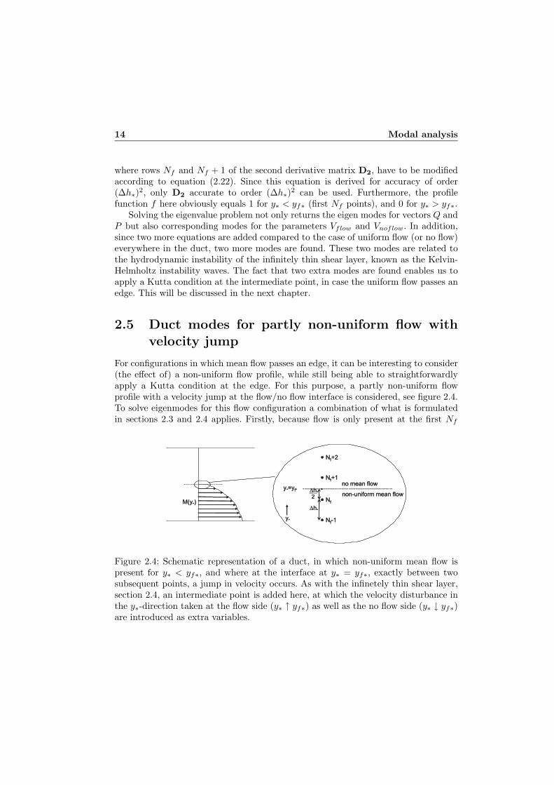
2.5 Duct modes for partly non-uniform flow withvelocity jump
For configurations in which mean flow passes an edge, it can be interesting to consider(the effect of) a non-uniform flow profile, while still being able to straightforwardlyapply a Kutta condition at the edge. For this purpose, a partly non-uniform flowprofile with a velocity jump at the flow/no flow interface is considered, see figure 2.4.To solve eigenmodes for this flow configuration a combination of what is formulatedin sections 2.3 and 2.4 applies. Firstly, because flow is only present at the first Nf
� �
�
�
� � � � � � � � � � � � � � � � � � �
� � � � � � � � � � �
� �
� � � � �
� � � � �� � �
� � ��
� �
�
�
� � � � � � � � � � � � � � � � � � �
� � � � � � � � � � �
� �
� � � � �
� � � � �� � �
� � ��
Figure 2.4: Schematic representation of a duct, in which non-uniform mean flow ispresent for y∗ < yf∗, and where at the interface at y∗ = yf∗, exactly between twosubsequent points, a jump in velocity occurs. As with the infinetely thin shear layer,section 2.4, an intermediate point is added here, at which the velocity disturbance inthe y∗-direction taken at the flow side (y∗ ↑ yf∗) as well as the no flow side (y∗ ↓ yf∗)are introduced as extra variables.

2.6 Classification of the modes 15
discrete points, only the equations with/for V at these points are kept. Secondly, aswith partly uniform flow, section 2.4, an extra point is introduced at the flow/no flowinterface, where the y-dependent part of pressure and velocity disturbance as seenfrom the flow side -Pflow, Vflow- as well as the no flow side -Pnoflow, Vnoflow- areconsidered. Analogous to equation (2.22) the second order derivative of the acousticpressure, accurate to order (∆h∗)2, amplitude at points Nf and Nf + 1 changes into:
d2P
dy2∗|Nf
=P(Nf − 1) − P(Nf )
(∆h∗)2− i(ω∗ −Mintk∗)Vflow
∆h∗,
d2P
dy2∗|Nf +1 =
−P(Nf + 1) + P(Nf + 2)(∆h∗)2
+iω∗Vnoflow
∆h∗, (2.28)
where Mint is the (jump in) Mach number at the interface. Unlike with the configura-tion of partly uniform flow, the first derivative also occurs in the eigenvalue problemfor the first Nf points here, since flow is non-uniform. The first order derivative ofthe acoustic pressure amplitude, accurate to order (∆h∗)2, at point Nf becomes:
dPdy∗
|Nf=
P(Nf ) − P(Nf − 1)2∆h∗
− i(ω∗ −Mintk∗)Vflow
2. (2.29)
Furthermore, adding continuity in pressure and displacement over the flow/no flowinterface in the eigenvalue problem yields the extra equations:
3i∆h∗Mintk∗Vflow = P(Nf − 1) − 9P(Nf ) + 9P(Nf + 1) − P(Nf + 2)+3i∆h∗ω∗Vflow + 3i∆h∗ω∗Vnoflow, (2.30)
andMintk∗Vnoflow = ω∗Vnoflow − ω∗Vflow, (2.31)
analoguous to (2.23) and (2.26). Generally, for this flow configuration N acousticmodes propagating/decaying in the +x-direction, N acoustic modes propagating/ordecaying in the −x-direction, Nf neutral hydrodynamic modes and 2 hydrodynamicinstability modes are found.
2.6 Classification of the modes
In the preceding part of this chapter the method to determine the modes for theacoustic pressure and velocity disturbance in a duct has been discussed for differentmean flow configurations. The existence of different types of modes, namely acousticmodes and hydrodynamic modes, is already mentioned there. Here, this distinctionwill be treated in more detail.

16 Modal analysis
Generally, acoustic modes propagate or decay along the fluid in both directions.The lowest order acoustic modes are the plane waves, which always have real wavenum-ber and therefore propagate. Higher order acoustic modes have a wavenumber withan imaginary part when they are ’cut-off’, such that they decay exponentially. Asalready mentioned in section 2.2 these will be found in complex conjugate pairs, ofwhich one decays in the +x direction and the other one decays in the −x direction.With increasing frequency ever more higher order modes are cut-on, such that theirwavenumbers become real and they will propagate. For a still fluid the wavenumbersof evanescent acoustic modes are purely imaginary, when mean flow is present thewavenumbers can have an additional real part. Hydrodynamic modes are associatedwith vorticity disturbances arising from shear in the mean flow. They are stationarywith respect to the fluid, i.e. they propagate with the (local) mean flow velocity. Hy-drodynamic modes can be either neutral, which means their wavenumber is purelyreal, or unstable, which means the wavenumber has an additional positive imaginarypart such that the mode grows exponentially in the direction of propagation (i.e.in the current exp(i(ωt − kx)) convention). An unstable hydrodynamic mode is alsoaccompanied with its complex conjugated counterpart, which decays exponentially.
Formally, when modes and their wavenumbers are calculated, the direction ofpropagation is not known. This especially becomes a relevant issue when an unstablehydrodynamic mode may be present, since it can be confused with an acoustic modedecaying in the −x direction, as both (can) have a wavenumber with positive realand imaginary part. In order to determine the direction of propagation of modes,two causality criteria are available, viz. the Briggs-Bers formalism [12, 18] and theCrighton-Leppington formalism [21, 49]. In both cases the wavenumbers of the modesare traced while letting the angular frequency ω go from a complex value to itseventual real value. In the Briggs-Bers formalism (ω) is kept constant while (ω)runs from −∞ to 0, whereas in the Crighton-Leppington formalism |ω| is fixed andarg(ω) runs from − 1
2π to 0, see figure 2.5. For the current exp(i(ωt−kx)) convention,if a wavenumber originates in the lower complex plane, the mode is right running, ifit originates in the upper complex plane the mode propagates to the left. This impliesthat if the wavenumber crosses the real axis the mode is unstable.
As an illustration wavenumber tracing is performed for a duct with partly uniformmean flow and a duct with partly non-uniform mean flow. For the first case uniformmean flow is present in the lower half of the duct and the fluid is quiescent in theupper half of the duct, such that the Mach number equals M(y∗) = M0f(y∗) with:
f(y∗) =
⎧⎨⎩
1 y∗ < 0.5,
0 y∗ > 0.5.
For the non-uniform flow case Poiseuille flow is present in the lower half of the duct

2.6 Classification of the modes 17
� � ��
� � � �
� � �
� � �
� � �� � � ��
� � � �� � � �
� � �
� � �
Figure 2.5: Variation of the angular frequency ω in the complex plane to its final realvalue for causality analysis according to Briggs-Bers formalism (B-B) and Crighton-Leppington formalism (C-L).
whereas the fluid is still in the upper half, such that M(y∗) = M0f(y∗) with:
f(y∗) =
⎧⎨⎩
32
(1 − (2y∗)2
)y∗ < 0.5,
0 y∗ > 0.5,
and M0 is here the Mach number averaged over the part with flow. For both casesthe dimensionless angular frequency is set at ω∗ = 0.2, M0 = 0.1 and a number ofN = 10 discrete points is taken. Figure 2.6 shows a plot of the two sample flow profilestogether with the location of the discrete points. The traces of the wavenumbers,divided by k0 = ω/c0, in the complex plane according to both the Briggs-Bers andthe Crighton-Leppington formalism are shown in figures 2.7 and 2.8 for the uniformand the non-uniform flow case respectively. Here, the two different causality criteriagive the same results regarding the direction of propagation of the modes. However,it has to be noted that Rienstra and Peake [96] have shown that for some cases theyactually disagree, and the Briggs-Bers formalism can not be used.
Generally, in this study the global aeroacoustic behaviour of two geometrical con-figurations will be studied at low frequency. This means that higher order modes willbe cut-off, and the aeroacoustical behaviour will be derived from the propagatingplane waves. Technically, for this purpose only a distinction between left running andright-running waves and the identification of the plane waves is needed. The planewaves could be discerned in a straightforward way by the form of the mode itself: they-dependent part of the pressure disturbance, P (y), will be almost constant and they-dependent part of the velocity disturbance in the y direction, V (y), will be nearlyzero. An identification of these modes on basis of their wavenumber can be made

18 Modal analysis
0 0.2 0.4 0.6 0.8 10
0.2
0.4
0.6
0.8
1
f
y*
(a)
0 0.4 0.8 1.2 1.60
0.2
0.4
0.6
0.8
1y
*
f
(b)
Figure 2.6: Sample flow profiles taken for the tracing of wavenumbers in the complexplane. a) partly uniform flow, b) partly non-uniform Poiseuille flow. The markers showthe locations of the N = 10 discrete points.
using the propagation velocity. The phase velocity of a mode is given by:
vp =ω
(k), (2.32)
which implies that:
( kk0
)=c0vp. (2.33)
The (quasi) plane waves propagate with the speed of sound c0 corrected with a Dopplershift due to the mean flow. The plane wave propagating to the left against mean flowwill thus have a velocity of about −c0(1− < M >), and the plane wave propagating tothe right with mean flow will have a velocity of about c0(1+ < M >), where < M > isthe mean flow Mach number averaged over the entire duct. For the sample flow casesabove, with a average Mach number of M0 in the lower half of the duct and zero meanflow in the upper half, the wavenumbers of the plane modes are expected to have avalues of k
k0= ± 1
1±0.5M0, or k
k0= −1.0526 and k
k0= 0.9524 respectively. Indeed, in
figures 2.7 and 2.8 values of kk0
= −1.0485 and kk0
= 0.9490 for the partly uniformflow configuration, and k
k0= −1.0476 and k
k0= 0.9473 for the partly non-uniform
flow configuration are found.As the hydrodynamic modes propagate with the local flow velocity, it is ex-
pected for the partly non-uniform flow configuration, that for these modes (k/k0) >

2.6 Classification of the modes 19
−10 −5 0 5 10 15 20 25 30
−100
−50
0
50
100
ℜ(k/k0)
ℑ(k/k0)
(a) Briggs-Bers formalism
−10 −5 0 5 10 15
−100
−50
0
50
100
ℜ(k/k0)
ℑ(k/k0)
(b) Crighton-Leppington formalism
Figure 2.7: Tracing of the wavenumbers for partly uniform flow (infinitely thin shearlayer) in a duct with w∗ = 0.2, M0 = 0.1, and N = 10 according to the Briggs-Bers formalism and the Crighton-Leppington formalism. The markers indicate theeventual values of the wavenumbers for real angular frequency. A classification is given:∗ marker: +x acoustic propagating, ∇ marker: −x acoustic propagating, + markers:+x acoustic evanescent, × markers: −x acoustic evanescent, � markers: hydrodynamicunstable/evanescent. Notice that in the C-L formalism the trace of the hydrodynamicevanescent mode coincides with part of the trace of the hydrodynamic unstable mode.

20 Modal analysis
−10 0 10 20 30 40
−100
−50
0
50
100
ℜ(k/k0)
ℑ(k/k0)
(a) Briggs-Bers formalism
−15 −10 −5 0 5 10 15 20
−100
−50
0
50
100
ℜ(k/k0)
ℑ(k/k0)
(b) Crighton-Leppington formalism
Figure 2.8: Tracing of the wavenumbers for partly non-uniform Poiseuille flow in aduct with w∗ = 0.2, M0 = 0.1, and N = 10 according to the Briggs-Bers formalismand the Crighton-Leppington formalism. The markers indicate the eventual values ofthe wavenumbers for real angular frequency. A classification is given: ∗ marker: +xacoustic propagating, ∇ marker: −x acoustic propagating, + markers: +x acousticevanescent, × markers: −x acoustic evanescent, ◦ markers: hydrodynamic neutral, �markers: hydrodynamic unstable/evanescent.

2.7 Comparison with analytical solutions 21
1/1.5M0 = 6.6667. Also, since they propagate in the direction of the mean flow, theymust originate in the lower complex wavenumber plane. Three of these modes, whichhave zero imaginary part, are found in figure 2.8. These are the neutral hydrody-namic modes. The neutral hydrodynamic mode with the smallest wavenumber has(k/k0) = 6.6673. Furthermore, one such mode is found, of which the wavenumbertrace has crossed the real axis to settle at a positive imaginary value. This is the hy-drodynamic unstable mode, which is accompanied by its decaying complex conjugatecounterpart. As expected, the total number of hydrodynamic modes found is thusfive: equal to the number of discrete points at which sheared mean flow is present.The rest of the modes are cut-off acoustic modes, all decaying in their direction ofpropagation. Notice that, according to the above, neutral hydrodynamic modes arealways expected at a higher wavenumber than the plane acoustic mode propagatingin +x-direction. A distinction can thus easily be made. This also extends to cut-onpropagating higher order acoustic modes, since these will have smaller wavenumbersthan the plane wave.
For the partly uniform flow configuration, besides the acoustic modes, two hydro-dynamic modes, an unstable one and its complex conjugate, are found. The value of(k/k0) equals 10.0317 for these modes, so that their phase velocity is close to themean flow velocity which has M0 = 0.1. These modes correspond to the well knownKelvin-Helmholtz instability waves, which will be discussed in more detail further on.
2.7 Comparison with analytical solutions
In order to investigate the accuracy of the modes and wavenumbers, obtained by themethod described above, results of calculations, carried out using a Matlab script, willbe compared to analytical solutions. Acoustic modes, hydrodynamic unstable modesand hydrodynamic neutral modes will be treated separately, as analytical solutionsfor these can only be obtained for different specific flow configurations.
2.7.1 Acoustic modes
In case of uniform mean flow in a duct, equation (2.14) reduces to:
(1 −M20 )k2
∗P + 2ω∗M0k∗P − ω2∗P − d2P
dy2∗= 0, (2.34)
which has the solution:
Pe,n(y∗) = cos((n− 1)πy∗),
ke,n∗ =−ω∗M0 ±
√ω2∗ − ((n− 1)π)2
1 −M20
, n ≥ 1, (2.35)
22 Modal analysis
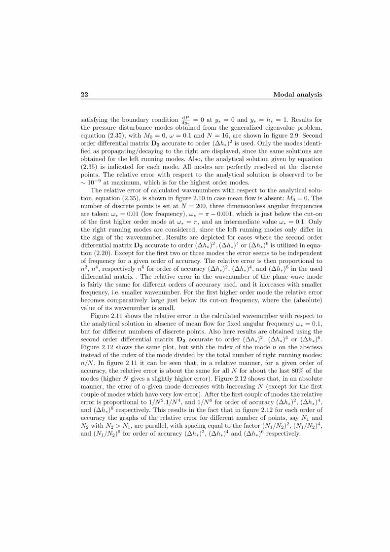
satisfying the boundary condition dPdy∗
= 0 at y∗ = 0 and y∗ = h∗ = 1. Results forthe pressure disturbance modes obtained from the generalized eigenvalue problem,equation (2.35), with M0 = 0, ω = 0.1 and N = 16, are shown in figure 2.9. Secondorder differential matrix D2 accurate to order (∆h∗)2 is used. Only the modes identi-fied as propagating/decaying to the right are displayed, since the same solutions areobtained for the left running modes. Also, the analytical solution given by equation(2.35) is indicated for each mode. All modes are perfectly resolved at the discretepoints. The relative error with respect to the analytical solution is observed to be∼ 10−9 at maximum, which is for the highest order modes.
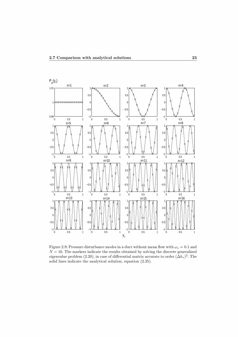
The relative error of calculated wavenumbers with respect to the analytical solu-tion, equation (2.35), is shown in figure 2.10 in case mean flow is absent: M0 = 0. Thenumber of discrete points is set at N = 200, three dimensionless angular frequenciesare taken: ω∗ = 0.01 (low frequency), ω∗ = π − 0.001, which is just below the cut-onof the first higher order mode at ω∗ = π, and an intermediate value ω∗ = 0.1. Onlythe right running modes are considered, since the left running modes only differ inthe sign of the wavenumber. Results are depicted for cases where the second orderdifferential matrix D2 accurate to order (∆h∗)2, (∆h∗)4 or (∆h∗)6 is utilized in equa-tion (2.20). Except for the first two or three modes the error seems to be independentof frequency for a given order of accuracy. The relative error is then proportional ton2, n4, respectively n6 for order of accuracy (∆h∗)2, (∆h∗)4, and (∆h∗)6 in the useddifferential matrix . The relative error in the wavenumber of the plane wave modeis fairly the same for different orders of accuracy used, and it increases with smallerfrequency, i.e. smaller wavenumber. For the first higher order mode the relative errorbecomes comparatively large just below its cut-on frequency, where the (absolute)value of its wavenumber is small.
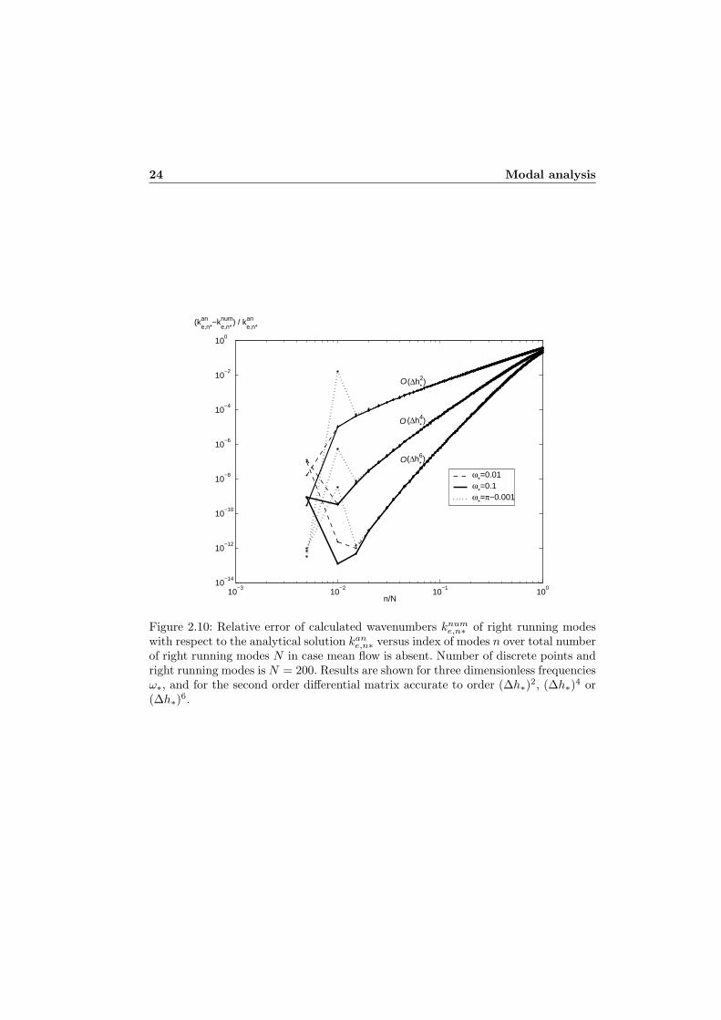
Figure 2.11 shows the relative error in the calculated wavenumber with respect tothe analytical solution in absence of mean flow for fixed angular frequency ω∗ = 0.1,but for different numbers of discrete points. Also here results are obtained using thesecond order differential matrix D2 accurate to order (∆h∗)2, (∆h∗)4 or (∆h∗)6.Figure 2.12 shows the same plot, but with the index of the mode n on the abscissainstead of the index of the mode divided by the total number of right running modes:n/N . In figure 2.11 it can be seen that, in a relative manner, for a given order ofaccuracy, the relative error is about the same for all N for about the last 80% of themodes (higher N gives a slightly higher error). Figure 2.12 shows that, in an absolutemanner, the error of a given mode decreases with increasing N (except for the firstcouple of modes which have very low error). After the first couple of modes the relativeerror is proportional to 1/N2,1/N4, and 1/N6 for order of accuracy (∆h∗)2, (∆h∗)4,and (∆h∗)6 respectively. This results in the fact that in figure 2.12 for each order ofaccuracy the graphs of the relative error for different number of points, say N1 andN2 with N2 > N1, are parallel, with spacing equal to the factor (N1/N2)2, (N1/N2)4,and (N1/N2)6 for order of accuracy (∆h∗)2, (∆h∗)4 and (∆h∗)6 respectively.
2.7 Comparison with analytical solutions 23
0 0.5 10.99
1
1.01
y*
Pe(y
*)
0 0.5 1−1
−0.5
0
0.5
1
0 0.5 1−1
−0.5
0
0.5
1
0 0.5 1−1
−0.5
0
0.5
1
0 0.5 1−1
−0.5
0
0.5
1
0 0.5 1−1
−0.5
0
0.5
1
0 0.5 1−1
−0.5
0
0.5
1
0 0.5 1−1
−0.5
0
0.5
1
0 0.5 1−1
−0.5
0
0.5
1
0 0.5 1−1
−0.5
0
0.5
1
0 0.5 1−1
−0.5
0
0.5
1
0 0.5 1−1
−0.5
0
0.5
1
0 0.5 1−1
−0.5
0
0.5
1
0 0.5 1−1
−0.5
0
0.5
1
0 0.5 1−1
−0.5
0
0.5
1
0 0.5 1−1
−0.5
0
0.5
1
n=1
n=6
n=2 n=3
n=5
n=4
n=8n=7
n=11n=10 n=9 n=12
n=13 n=14 n=15 n=16
Figure 2.9: Pressure disturbance modes in a duct without mean flow with ω∗ = 0.1 andN = 16. The markers indicate the results obtained by solving the discrete generalizedeigenvalue problem (2.20), in case of differential matrix accurate to order (∆h∗)2. Thesolid lines indicate the analytical solution, equation (2.35).
24 Modal analysis
10−3
10−2
10−1
100
10−14
10−12
10−10
10−8
10−6
10−4
10−2
100
n/N
(kane,n*
−knume,n*
) / kane,n*
ω*=0.01
ω*=0.1
ω*=π−0.001
(∆h*2)
(∆h*4)
(∆h*6)
O
O
O
Figure 2.10: Relative error of calculated wavenumbers knume,n∗ of right running modes
with respect to the analytical solution kane,n∗ versus index of modes n over total number
of right running modes N in case mean flow is absent. Number of discrete points andright running modes is N = 200. Results are shown for three dimensionless frequenciesω∗, and for the second order differential matrix accurate to order (∆h∗)2, (∆h∗)4 or(∆h∗)6.

2.7 Comparison with analytical solutions 25
10−3
10−2
10−1
100
10−14
10−12
10−10
10−8
10−6
10−4
10−2
100
n/N
(kane,n*
−knume,n*
) / kane,n*
N=50N=200N=800
(∆h*2)
(∆h*4)
(∆h*6)
O
O
O
Figure 2.11: Relative error of calculated wavenumbers knume,n∗ of right running modes
with respect to the analytical solution kane,n∗ versus index of modes n over total number
of right running modes N in case mean flow is absent. Dimensionless frequency isω∗ = 0.1. Results are shown for three numbers of discrete points N , and for thesecond order differential matrix accurate to order (∆h∗)2, (∆h∗)4 or (∆h∗)6.
26 Modal analysis
100
101
102
103
10−14
10−12
10−10
10−8
10−6
10−4
10−2
100
n
(kane,n*
−knume,n*
) / kane,n*
O(∆h*2)
O(∆h*4)
O(∆h*6)
N=50 N=200 N=800
Figure 2.12: Relative error of calculated wavenumbers knume,n∗ of right running modes
with respect to the analytical solution kane,n∗ in case mean flow is absent. Dimensionless
frequency is ω∗ = 0.1. Plot is identical to figure 2.11, but with index n of the modeson abscissa instead of n/N .
2.7 Comparison with analytical solutions 27
2.7.2 Unstable hydrodynamic modes
Hydrodynamic modes are associated with shear in the mean flow rather than withcompressibility of the medium, as applies for acoustic modes. As mentioned, thesemodes can be stable as well as unstable.
The configuration of two parallel infinite streams of incompressible inviscid fluidswith different velocities and densities was recognized by Helmholtz [38], whereas theaccompanying problem of instability was first posed and solved by Kelvin [51]. It isnow commonly known as the Kelvin-Helmholtz instability for an infinitely thin shearlayer, see also e.g. ref. [11, 29]. The hydrodynamic modes and wavenumbers for aninfinitely thin shear layer in an incompressible fluid with homogeneous density can bereadily solved analytically. Results will be compared to those obtained by the presentmodal analysis method.
For continuous parallel flows Rayleigh [92] first proved that the presence of aninflexion point in the flow profile is a necessary condition for instability. Subsequentlystronger criteria have been derived by others, see for instance Drazin and Reid [29]. Fora generalized hyperbolic-tangent flow profile hydrodynamic modes and wavenumbersare obtained by Michalke [67, 68, 69] by numerically solving the Rayleigh equation,see appendix B. Also comparison of these results with those obtained by the presentmodal analysis method will be made.
Infinitely thin shear layer
When fluid is considered to be incompressible, the Euler equation for conservation ofmass (2.2) changes into: −→∇ · −→v = 0. (2.36)
The incompressible variant of equation (2.14) can subsequently be deduced in thesame way as in section 2.2:
(k2∗ −
d2
dy2∗
)P = −2iM0
dfdy∗
k∗V, (2.37)
while equation (2.13) remains unchanged. In case of a duct with partly uniform meanflow, i.e. an infinitely thin shear layer, for which the flow profile f is given in figure2.6a, the right hand side of (2.37) equals 0 except at the shear layer itself. The solutionfor the pressure mode, beneath- respectively above the shear layer, is then given by:
Phu(y∗) =
⎧⎨⎩
cosh(khu∗y∗) y∗ < 0.5,
cosh(khu∗(y∗ − 1)) y∗ > 0.5.(2.38)
Here the boundary condition dPdy∗
= 0 at the duct walls at y∗ = 0 and y∗ = h∗ = 1,as well as continuity of pressure at y∗ = 0.5 is satisfied. Furthermore, in the same

28 Modal analysis
way as in section 2.4, continuity of displacement δ∗ is imposed over the shear layer.Equations (2.25) and (2.13) give for the y-dependant part of the displacement:
D(y∗) =1
(ω∗ −M0fk∗)2dPdy∗
. (2.39)
After substitution of equation (2.38) in (2.39), continuity of D at y∗ = 0.5 implies forthe wavenumber:
khu∗ =w∗M0
(1 ± i). (2.40)
The solution given by equations (2.38) and (2.40) is well known as the Kelvin-Helmholtz instability waves for a infinitely thin vortex sheet. The solution by modalanalysis is obtained from the generalized eigenvalue problem in the form given byequation (2.27), which is accurate to order (∆h∗)2. In order to approximate the in-compressible limit both the square of the dimensionless angular frequency and theMach number should be small: w2
∗ � 1 and M20 � 1. Figures 2.13, 2.14 and 2.15
show the unstable hydrodynamic pressure mode obtained from modal analysis com-pared to the incompressible analytical solution, equations (2.38,2.40), for ω∗ = 0.1 andM0 = 0.1, for ω∗ = 0.01 and M0 = 0.01, and for ω∗ = 0.1 and M0 = 0.01 respectively.In all cases the number of discrete points is N = 50. The maximum of the absolutevalue of the pressure mode, |Phu|, is scaled to unity. Note that the decaying hydro-dynamic pressure mode only differs from the unstable one by an opposite phase. For
0 0.2 0.4 0.6 0.8 10.975
0.98
0.985
0.99
0.995
1
1.005
|Phu
|
y*
0 0.2 0.4 0.6 0.8 1−0.05
0
0.05
0.1
0.15
0.2
0.25
0.3
arg(Phu
) (rad)
y*
Figure 2.13: Magnitude and phase of the unstable hydrodynamic pressure wave Phu
for an infinitely thin shear layer obtained from modal analysis (× markers) comparedto the incompressible analytical solution (solid line) for ω∗ = 0.1, M0 = 0.1, N = 50.The maximum of |Phu| is scaled to unity.

2.7 Comparison with analytical solutions 29
0 0.2 0.4 0.6 0.8 10.975
0.98
0.985
0.99
0.995
1
1.005
y*
|Phu
|
0 0.2 0.4 0.6 0.8 1−0.05
0
0.05
0.1
0.15
0.2
0.25
0.3
arg(Phu
) (rad)
y*
Figure 2.14: Magnitude and phase of the unstable hydrodynamic pressure wave Phu
for an infinitely thin shear layer obtained from modal analysis (× markers) comparedto the incompressible analytical solution (solid line) for ω∗ = 0.01,M0 = 0.01,N = 50.The maximum of |Phu| is scaled to unity.
0 0.2 0.4 0.6 0.8 10
0.1
0.2
0.3
0.4
0.5
0.6
0.7
0.8
0.9
1
|Phu
|
y*
0 0.2 0.4 0.6 0.8 10
1
2
3
4
5
6
arg(Phu
) (rad)
y*
Figure 2.15: Magnitude and phase of the unstable hydrodynamic pressure wave Phu
for an infinitely thin shear layer obtained from modal analysis (× markers) comparedto the incompressible analytical solution (solid line) for ω∗ = 0.1, M0 = 0.01, N = 50.The maximum of |Phu| is scaled to unity.
30 Modal analysis
ω∗ = 0.1 and M0 = 0.1 clearly a deviation from the incompressible analytical solutioncan be seen, especially for the magnitude of the mode. For ω∗ = 0.01 and M0 = 0.01very good agreement between the result from modal analysis and the analytical so-lution is observed: the relative error is at maximum ∼ 10−5 for both magnitude andphase. When only the Mach number is small: M0 = 0.01, while ω∗ = 0.1, cf. figure2.15, agreement between modal analysis and the incompressible solution is also quitegood with a maximum relative error of ∼ 10−5 for magnitude and phase. When takingω∗ smaller than 0.1 while keeping M0 at 0.1 more significant deviation was seen. Ap-parently, the approximation of the incompressible limit by the modal analysis resultis more sensitive to the Mach number than the dimensionless frequency (Helmholtznumber). This is also seen in figure 2.16, where the deviation in the wavenumberof the hydrodynamic instability, when comparing the modal analysis result and theincompressible analytical solution, is plotted against both Mach number M0 and di-mensionless angular frequency ω∗ for N = 50. For the real part of the wavenumberthe deviation is almost independent of the dimensionless frequency. The deviation ofthe imaginary part however does depend on both Mach number and dimensionlessfrequency. Along the path where ω∗ is kept equal to M0 the deviation in both real andimaginary part is found to increase with the square of ω∗ = M0. For a higher numberof points N no significantly different result as in figure 2.16 was found, indicating thatthe calculation has converged.
Generalized hyperbolic-tangent shear layer profile
The spatial instability of a free shear layer with a more realistic flow profile wasinvestigated by Michalke [67, 68, 69], see also appendix B. He numerically solvedthe (incompressible) Rayleigh equation for a generalized hyperbolic-tangent velocityprofile, equation (B.8), to obtain the wavenumber khu of the hydrodynamic instabilitywave. In the current non-dimensionalization this flow profile is given by:
f(y∗) = 1 − (1 +memφ(m) y∗−0.5θ∗ )−1/m,
φ(m) =∫ 1
0
1 − z
1 − zmdz, (2.41)
with m a profile parameter and θ∗ = θ/h the non-dimensional momentum thicknessof the shear layer. Here, the inflexion point of the profile is set at y∗ = 0.5. Note thatin Michalke’s formulation the y-coordinate extends from −∞ to +∞, as opposed tothe restriction of y to the duct region in modal analysis.
Calculations are performed for profile parameter m = 1 and m = 6, using differen-tial matrices accurate to order O(∆h2
∗). For the momentum thickness three differentvalues are taken: θ∗ = 0.025, θ∗ = 0.05, and θ∗ = 0.1. The profiles for these parametervalues are displayed in figure 2.17. The hydrodynamic instability wavenumbers, non-dimensionalized by the momentum thickness, obtained from modal analysis are shown

2.7 Comparison with analytical solutions 31
10−3
10−2
10−1
100
10−3
10−2
10−1
100
10−7
10−6
10−5
10−4
10−3
10−2
10−1
ω*
M0
num an an
|(ℜ(khunum) −ℜ(k
huan)) / ℜ(k
huan)|
10−3
10−2
10−1
100
10−3
10−2
10−1
100
10−10
10−8
10−6
10−4
10−2
ω*
M0
|(ℑ(khunum) −ℑ(k
huan)) / ℑ(k
huan)|
Figure 2.16: Relative deviation in the real and imaginary part of the wavenumber khu∗of the unstable hydrodynamic wave for an infinitely thin shear layer when comparingthe modal analysis result (superscript num) and the incompressible analytical solutionsuperscript (an). Here N = 50, but virtually the same result was found for higher N .

32 Modal analysis
0 0.2 0.4 0.6 0.8 10
0.1
0.2
0.3
0.4
0.5
0.6
0.7
0.8
0.9
1
f
y*
(a) m=1
0 0.2 0.4 0.6 0.8 10
0.1
0.2
0.3
0.4
0.5
0.6
0.7
0.8
0.9
1
f
y*
(b) m=6
Figure 2.17: Generalized hyperbolic-tangent velocity profile, eq (2.41), in a duct forprofile parameters m = 1 and m = 6, and for non-dimensional momentum thicknessθ∗ = 0.1 (dashed line), θ∗ = 0.05 (solid line), and θ∗ = 0.025 (dotted line).
in figures 2.18 and 2.19 for m = 1 and m = 6 respectively. On the horizontal axesis the Strouhal number based on the momentum thickness ωθ/U0, with U0 = M0c0.The results of Michalke [67] are indicated by the solid lines. The dimensionless an-gular frequency is set at ω∗ = 0.01 in the calculations. Results of calculations withsmaller ω∗ and hence smaller M0 gave no significant difference, assuring sufficientapproximation of the incompressible limit. Furthermore, the spacing between discretepoints is kept constant with respect to θ∗ at ∆h∗/θ∗ = 0.1. This implies N = 100,N = 200, and N = 400 for θ∗ = 0.025, θ∗ = 0.05, and θ∗ = 0.1 respectively. Resultswere found to be converged ’visually’ for these numbers of discrete points in all cases.For both flow profile parameters good agreement between modal analysis results andMichalke’s results are observed for the smallest momentum thickness to duct heightratio: θ∗ = 0.025. For larger θ∗ significant deviation is seen, especially for profile pa-rameter m = 1 case and at low Strouhal numbers. The results thus confirm that inthe incompressible limit the modal analysis result for the wavenumber of the hydro-dynamic instability approaches Michalke’s result for a generalized hyperbolic-tangentshear layer unbounded in the y-direction, if the duct hight compared to momentumthickness is sufficiently large.

2.7 Comparison with analytical solutions 33
0 0.05 0.1 0.15 0.2 0.250
0.1
0.2
0.3
0.4
0.5
ωθ/U0
ℜ(khu
)θ
0 0.05 0.1 0.15 0.2 0.250
0.0025
0.05
0.075
0.1
0.125
ωθ/U0
ℑ(khu
)θ
Figure 2.18: Real and imaginary part of the wavenumber khu of the unstable hydro-dynamic mode versus Strouhal number for the hyperbolic- tangent profile, eq. (2.41),with m = 1. Modal analysis calculation are with ω∗ = 0.01 and dimensionless mo-mentum thickness θ∗ = 0.025 (+), θ∗ = 0.05 (∗) and θ∗ = 0.1 (×). The solid linerepresents a fit of the incompressible result found by Michalke [67]. The spacing be-tween discrete points is kept constant with respect to θ∗ at ∆h∗/θ∗ = 0.1, implyingN = 400, N = 200 and N = 100 respectively.

34 Modal analysis
0 0.05 0.1 0.15 0.2 0.250
0.1
0.2
0.3
0.4
0.5
0.6
0.7
0.8
0.9
ωθ/U0
ℜ(k)θ
0 0.05 0.1 0.15 0.2 0.250
0.05
0.1
0.15
0.2
0.25
ωθ/U0
ℑ(k)θ
Figure 2.19: Real and imaginary part of the wavenumber khu of the unstable hydro-dynamic mode versus Strouhal number for the hyperbolic- tangent profile, eq. (2.41),with m = 6. Modal analysis calculation are with ω∗ = 0.01 and dimensionless mo-mentum thickness θ∗ = 0.025 (+), θ∗ = 0.05 (∗) and θ∗ = 0.1 (×). The solid linerepresents a fit of the incompressible result found by Michalke [67]. The spacing be-tween discrete points is kept constant with respect to θ∗ at ∆h∗/θ∗ = 0.1, implyingN = 400, N = 200 and N = 100 respectively.

2.7 Comparison with analytical solutions 35
2.7.3 Neutral hydrodynamic modes
In the preceding sections, in which acoustic and hydrodynamic unstable modes wereconsidered, the quantity ω∗ −M0fk∗ did not vanish. However, when ω∗ −M0fk∗ = 0at a certain point ys∗, such that k∗ = ω∗/M0f(ys∗) , the Pridmore-Brown equation(2.19) is singular at y∗ = ys∗. Generally, the solution for P in the vicinity of thesingular point is found as a series development by substituting a Taylor expansion ofω∗ −M0fk∗ around y∗ = ys∗ in the Pridmore-Brown equation, see e.g. Lees and Lin[61]. Clearly, since 0 ≤ ys∗ ≤ 1, a continuous hydrodynamic spectrum with purely realwavenumbers ω∗/M0fmax ≤ khs∗ ≤ ω∗/M0fmin is obtained for non-uniform flow. Thiscontinuous set of modes is analyzed by e.g. Swinbanks [107]. In the present discretizedmodal analysis hydrodynamic neutral modes are expected to have wavenumbers withvalue khs∗ = ω∗/M0f(y∗) at the discrete points.
For a duct with a Poiseuille mean flow profile the calculated wavenumbers, usingdifferential matrices accurate to order ∆h2
∗, are compared with the expected valuesat the discrete points. Figure 2.20 shows the calculated values of k0/M0khs, which isequal to the phase velocity of the modes divided by the average main flow velocity U0.The values should coincide with the profile function f , also plotted in the figure, at thediscrete points. Indeed excellent agreement is seen, the relative deviation is in the orderof machine precision (O(10−16)). Note that, as no hydrodynamic instability occurs forsuch profile, all of the hydrodynamic modes found are neutral. The same comparisonis made for a duct with Poiseuille mean flow only in the lower half (see also figure2.6b). Figure 2.21 shows the results for a Mach number at which no hydrodynamicinstability occurs and for a higher Mach number where also hydrodynamic unstablemodes are present. When no hydrodynamic instability is found, the wavenumbers ofthe neutral modes again perfectly agree with the expected values at all discrete points.In case hydrodynamic instability occurs two of the calculated hydrodynamic modesare unstable, leaving two less solved neutral modes. The wavenumber values for theseneutral modes are in agreement with the expected value, but the neutral modes withphase velocity corresponding with the flow velocity at the two discrete points justbefore the mean flow to no mean flow transition are not found.
Also hydrodynamic neutral modes for the hyperbolic-tangent shear layer profile,equation (2.41), with profile parameter m = 1 are considered. For this case the devi-ation in wavenumber turns out to be more significant. Figure 2.22 shows the relativeerror of the calculated wavenumbers of the hydrodynamic neutral modes knum
hs withrespect to the expected analytical value kan
hs versus the discrete points in y∗. The di-mensionless frequency is ω∗ = 0.01 and the momentum thickness to duct height ratiois θ∗ = 0.025. This flow profile is also considered in the previous section and is shownin figure 2.17a. The Strouhal number is chosen ωθ/U0 = 0.3, such that no hydrody-namic instability occurs, see figure 2.18. Calculations are performed using differentialmatrices accurate to order ∆h2
∗ (fig.2.22a), ∆h4∗ (fig.2.22b) and ∆h6
∗ (fig.2.22c) atdifferent number of discrete points N . For the O(∆h4
∗) and O(∆h6∗) calculations con-

36 Modal analysis
0 0.2 0.4 0.6 0.8 1 0
0.5
1
1.5f, k
0/M
0k
hs
y*
Figure 2.20: Calculated values of the hydrodynamic neutral wavenumbers khs for aduct with Poiseuille mean flow plotted as k0/M0khs (× markers) coincide with thevalue of the profile function f at the discrete points (◦ markers). Parameter valuesare ω∗ = 0.1, N = 50, M0 = 0.1
vergence in the wavenumber deviation is -at least visually- established at N = 200.For the O(∆h2
∗) calculations are done up to N = 500, where convergence in thewavenumber deviation was no yet completely observed. The wavenumber deviationagainst position y∗ for the different orders of accuracy, each at the highest numberof points N used, are shown together in figure 2.22d. The largest deviation in thewavenumbers is seen in the region of the actual shear layer, where mean flow velocitychanges most rapidly. However, halfway the duct at the inflexion point, where shearis maximum, a local minimum in the wavenumber deviation is seen. The error in thewavenumber versus position is quite similar for the O(∆h4
∗) and O(∆h6∗) calculations,
whereas the O(∆h2∗) calculation additionally shows relatively large error in the lower
half of the shear layer. Remarkably, the error in the wavenumbers for the O(∆h4∗)
calculation is in general smaller than for the O(∆h6∗) calculation.

2.7 Comparison with analytical solutions 37
0 0.2 0.4 0.6 0.8 1 0
0.5
1
1.5f, k
0/M
0k
hs
y*
(a) no hydrodynamic instability
0 0.2 0.4 0.6 0.8 1 0
0.5
1
1.5f, k
0/M
0k
hs
y*
(b) hydrodynamic instability
Figure 2.21: Calculated values of the hydrodynamic neutral wavenumbers khs for aduct with Poiseuille mean flow only in the lower half plotted as k0/M0khs (× marker)coincide with the value of the profile function f at the discrete points (◦ markers).(a) Average Mach number is M0 = 0.02: no hydrodynamic instability occurs, neutralhydrodynamic modes are solved at all discrete points. (b) M0 = 0.1: hydrodynamicinstability occurs and consequently two less neutral hydrodynamic modes, at the twodiscrete points before the flow/no flow transition, are solved. Other parameters areω∗ = 0.2 and N = 100

38 Modal analysis
0 0.2 0.4 0.6 0.8 1 0
0.005
0.01
0.015
0.02
0.025
0.03
y*
|(khsnum−k
hsan)/k
hsan|
N=300N=400N=500
(a)
0 0.2 0.4 0.6 0.8 1 0
1
2
3
4
5
6
7
8x 10
−3
y*
|(khsnum−k
hsan)/k
hsan|
N=50N=100N=200
(b)
0 0.2 0.4 0.6 0.8 1 0
0.001
0.002
0.003
0.004
0.005
0.006
0.007
0.008
0.009
0.01
y*
|(khsnum−k
hsan)/k
hsan|
N=50N=100N=200
(c)
0 0.2 0.4 0.6 0.8 1 0
0.002
0.004
0.006
0.008
0.01
0.012
0.014
0.016
0.018
y*
|(khsnum−k
hsan)/k
hsan|
O(∆h2)O(∆h4)O(∆h6)
(d)
Figure 2.22: Relative error of the calculated wavenumbers of the hydrodynamic neutralmodes knum
hs with respect to the expected analytical value kanhs versus the discrete
points in y∗ for a hyperbolic-tangent shear layer profile, eq. (2.41), with m = 1.Furthermore ω∗ = 0.01 and θ∗ = 0.025. This flow profile is also given in figure2.17a. Calculations are done at different number of discrete points N for differentialmatrices accurate to order O(∆h2
∗) (a), O(∆h4∗) (b) and O(∆h6
∗) (c). (d) shows resultsfor different orders of accuracy together, each for the highest number N .

2.8 Conclusion 39
2.8 Conclusion
A finite difference method to obtain a discrete generalized eigenvalue problem for thetransverse modes and their accompanying wavenumbers for the linear pressure andvelocity disturbance in a two dimensional rectangular duct with parallel shear flowhas been presented. Application of the method to some particular shear layer profiles,which will be considered in flow configurations further on, is treated in more detail.Causality criteria to discern the direction of propagation of the modes as well as aclassification in acoustic (propagating or evanescent) and hydrodynamic (unstable orneutral) modes are discussed. In absence of mean flow the analytically well knownmodes are resolved perfectly at the discrete points and good convergence of the calcu-lated wavenumber to the analytical values is observed. For an infinitely thin shear layerthe calculated modes and wavenumbers of the hydrodynamic instability approach theincompressible analytical solution well for low Helmholtz and Mach number. Also, inthe incompressible limit, the wavenumbers of the unstable hydrodynamic modes fora generalized hyperbolic-tangent shear layer profile are found to be in good agree-ment with the solution obtained by Michalke [67, 68, 69], where the shear layer is notbounded perpendicular to the flow direction, provided that shear layer momentumthickness to duct height ratio is sufficiently small (about 0.025). The continuum ofneutral hydrodynamic modes with phase velocities corresponding to the mean flow ve-locity is solved at the discrete points. For a duct with (partly) non uniform Poiseuilleflow the calculated wavenumbers perfectly agree with the expected values. However,when hydrodynamic instability occurs, the two neutral hydrodynamic modes withphase velocity corresponding to the mean flow velocity at the discrete points closestto the flow to no flow transition are not resolved anymore ’in favour’ of the two un-stable modes. For the hyperbolic-tangent profile more significant deviation is seen forthe calculated wavenumbers of neutral hydrodynamic modes which correspond to theregion where shear is largest.


Chapter 3
Area expansion in a duct:modal analysis
3.1 Introduction
Perhaps the most simple duct configuration, in which a shear layer is formed, is thatof a sudden area expansion in a two-dimensional duct with mean flow. Technical ap-plications are internal combustion engine exhaust silencers and silencers in industrialduct systems.
Probably the most extensive experimental work on this topic is that of Ron-neberger [100]. He presented results for both magnitude and phase of the reflection-as well as transmission coefficients of the acoustic plane pressure waves at an areaexpansion in a cylindrical duct with anechoic termination.
Early models to describe the acoustical properties of an area expansion in a ductwith flow are that of Ronneberger [97] and Alfredson and Davies [3]. Here, in a low-frequency plane wave approximation, one-dimensional linearized equations for theconservation of mass, momentum and energy are applied to a control volume aroundthe area expansion. Dissipation is accounted for by entropy fluctuations, associatedwith the formation of vortices in the mixing region downstream of the expansion,which is thus included in the control volume. Alfredson and Davies [3] comparedtheoretical prediction and experimental data for the reflection coefficient up to aMach number of 0.15, reasonable agreement was found. Ronneberger [97] comparedpredicted and measured results for the reflection coefficient up to Mach numbers of0.6, but also here only good agreement was obtained for Mach numbers below ∼0.15.Cummings [23] proposed a similar model, in which scattering is assumed to occur inthe control volume, where the flow has not yet expanded, while energy losses due to thevorticity are now accounted for by entropy waves downstream of the control volume.

42 Area expansion in a duct: modal analysis
Comparison with Ronneberger’s experimental results yielded better agreement forthe higher Mach numbers. Furthermore, in a later correspondence [24] he concludedthat entropy fluctuations need not to be taken into account as they are of secondaryimportance and probably are negligible compared to higher order modes and shearflow effects. All of the above mentioned models lack the effects of higher order modesas they are low-frequency (plane wave) approximations.
Lambert and Steinbrueck [59] proposed a low frequency, low Mach number modelon the basis of the statement that the magnitude of the reflection coefficient at anarea expansion is only Mach number dependent, whereas its phase is only frequencydependent. The magnitude is calculated from applying conservation equations to acontrol volume around the area expansion, in which the mean flow has expanded. Thephase is calculated from an equivalent end correction for no mean flow [50]. Davies [26]proposed a similar model where the phase is calculated from either an equivalent endcorrection or by including higher order modes in the matching of the ducts upstreamand downstream of the area expansion. The use of an equivalent end correction forthe phase of the reflection coefficient was extended to higher frequencies by Peat [85],who also compared results of the analytical model with a finite element method. It hasto be noted here, that the, in these models, assumed dependency of magnitude andphase of the reflection coefficient on only Mach number respectively only frequencyis actually in contradiction with (for example) experimental results of Ronneberger[100] and theoretical results of Boij and Nilsson [16] (see also below). Also, in theclosely related problems of reflection at an open pipe with mean flow and scatteringat a diaphragm in a pipe with mean flow the magnitude and phase is found to bedependent on both Mach number and frequency. This was shown experimentally byPeters [87] and Allam and Abom [4] and theoretically by Munt [77, 78], Rienstra [95]and Cargill [19] for the open pipe, and by e.g. Hofmans [42] and Testud [109] for thediaphragm.
Auregan [5, 7] presented a simplified multi-modal model for the aero-acousticbehaviour of a sudden area expansion at low frequency in a cylindrical duct. Theuniform mean flow was considered to remain unexpanded after the area discontinu-ity. The effect of entropy fluctuations due to mixing downstream of the expansion isnot accounted for. The acoustic pressure and radial velocity field downstream of theexpansion was expanded into six modes assuming a prescribed form [106]: a planewave mode and a mode accounting for higher-order effects in either direction of prop-agation, and two hydrodynamic modes. Subsequently, applying continuity of meanacoustic pressure and volume flux and a Kutta condition at the area discontinuitygave the acoustic behaviour. A favourable comparison of the predicted magnitudeof the reflection coefficient with the experimental results of Ronneberger [100] wasshown.
An alternative method was given by Dupere and Dowling [30]. They described theinteraction of the shear layer with the sound field by means of an acoustic analogy,

3.1 Introduction 43
in which the shear layer acts as a source/sink term in the wave equation in thedownstream duct. Note that this is similar to the method of Howe for the acousticalresponse of a shear layer in a wall aperture, extensively described in appendix A. Inthe model of Dupere and Dowling the Mach number is very low and the shear layeris assumed to be thick, such that hydrodynamic instability does not occur.
Recently, Boij and Nilsson [16] presented a model for the scattering at an areadiscontinuity in a rectangular two-dimensional duct carrying uniform mean flow. Alsoin this model the flow is considered to remain unexpanded after the area discontinuity.Higher order acoustic modes and hydrodynamic modes are taken into account, andthe problem is solved with the Wiener-Hopf technique with application of a Kuttacondition at the edge of the area discontinuity. A favourable comparison for the scat-tering coefficients with experimental results of Ronneberger [97, 100] is made. For thispurpose a normalization of the Helmholtz number for both rectangular and cylindri-cal ducts is proposed. In a later paper [17] they addressed the issue of (in)stability ofthe vortex sheet. As the mean flow is assumed to be uniform and continues unalteredafter the expansion, an infinitely thin shear layer forms. As discussed in e.g. section2.4 of this thesis such a vortex sheet is always unstable. However, a real shear layerwith finite thickness becomes stable for sufficiently large Strouhal numbers. This isseen for instance for the hyperbolic-tangent profile discussed in appendix B.2. Boijand Nilsson accounted for this physical effect by suppressing the hydrodynamic insta-bility mode for higher Strouhal numbers. This was done by introducing a graduallyrelaxed Kutta condition at the edge, with empirical coefficients as to give a betterfit with experimental results for the downstream reflection coefficient. They reportedthat the effect of the relaxed Kutta condition on the downstream transmission coef-ficient is negligible. In the same paper they also calculate the absorption of energyat the area expansion, either accounting for the expansion of the flow downstream ofthe area discontinuity or not accounting for it.
In this chapter modal analysis, as described in the preceding chapter, is appliedto solve the aeroacoustical behaviour of a sudden area expansion in a duct. As in themodel of Auregan [5, 7] and Boij and Nilsson [16] the contribution of entropy wavesdue to the expansion of the flow downstream of the area discontinuity is neglectedhere. Besides the possibility of comparison with other models and experiments fromliterature, especially the established convergence of this method for this particular ge-ometry was motivating. First, the related mode matching will be treated for differentflow configurations. Subsequently, the effect of the mean flow profile and applicationof a Kutta condition is investigated. Furthermore, results are compared with thoseobtained by Boij and Nilsson [16, 17] and with experiments by Ronneberger [100].Specifically, in the light of the Helmholtz number scaling proposed by Boij and Nils-son [16] as mentioned above, a comparison between results for a two-dimensionalrectangular and a two-dimensional cylindrical geometry is made.
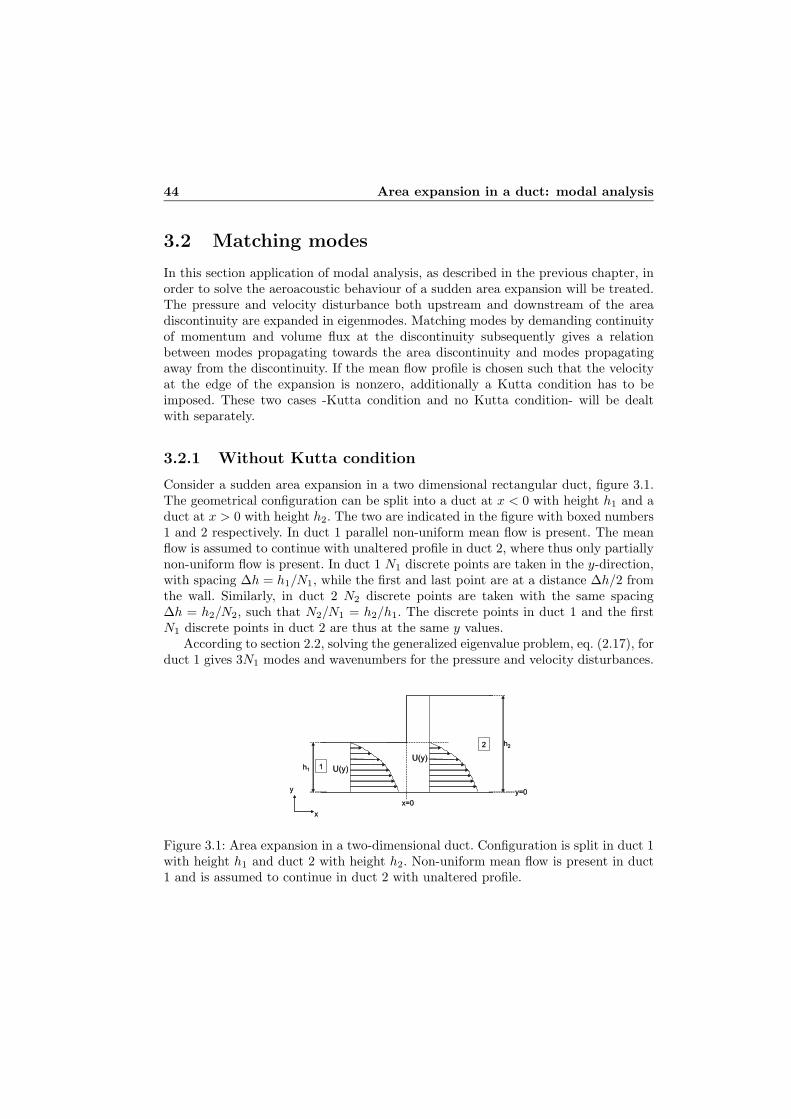
44 Area expansion in a duct: modal analysis
3.2 Matching modes
In this section application of modal analysis, as described in the previous chapter, inorder to solve the aeroacoustic behaviour of a sudden area expansion will be treated.The pressure and velocity disturbance both upstream and downstream of the areadiscontinuity are expanded in eigenmodes. Matching modes by demanding continuityof momentum and volume flux at the discontinuity subsequently gives a relationbetween modes propagating towards the area discontinuity and modes propagatingaway from the discontinuity. If the mean flow profile is chosen such that the velocityat the edge of the expansion is nonzero, additionally a Kutta condition has to beimposed. These two cases -Kutta condition and no Kutta condition- will be dealtwith separately.
3.2.1 Without Kutta condition
Consider a sudden area expansion in a two dimensional rectangular duct, figure 3.1.The geometrical configuration can be split into a duct at x < 0 with height h1 and aduct at x > 0 with height h2. The two are indicated in the figure with boxed numbers1 and 2 respectively. In duct 1 parallel non-uniform mean flow is present. The meanflow is assumed to continue with unaltered profile in duct 2, where thus only partiallynon-uniform flow is present. In duct 1 N1 discrete points are taken in the y-direction,with spacing ∆h = h1/N1, while the first and last point are at a distance ∆h/2 fromthe wall. Similarly, in duct 2 N2 discrete points are taken with the same spacing∆h = h2/N2, such that N2/N1 = h2/h1. The discrete points in duct 1 and the firstN1 discrete points in duct 2 are thus at the same y values.
According to section 2.2, solving the generalized eigenvalue problem, eq. (2.17), forduct 1 gives 3N1 modes and wavenumbers for the pressure and velocity disturbances.
�
�
� � � �� �
� � � �
� �
� � �
�
�
� � ��
�
� � � �� �
� � � �
� �
� � �
�
�
� � �
Figure 3.1: Area expansion in a two-dimensional duct. Configuration is split in duct 1with height h1 and duct 2 with height h2. Non-uniform mean flow is present in duct1 and is assumed to continue in duct 2 with unaltered profile.

3.2 Matching modes 45
Both N1 acoustic and N1 hydrodynamic modes propagating in the +x-direction andN1 acoustic modes propagating in the −x-direction are found. The generalized eigen-value problem for the modes in duct 2 has to be solved according to section 2.3. Anumber of N2 acoustic modes propagating in either direction and N1 hydrodynamicmodes are found here. The modes for the velocity disturbance are only defined at thefirst N1 points, where mean flow is present.
At the interface between the two ducts at x = 0 continuity of mass flux and mo-mentum applies. As derived in appendix D this yields continuity of the dimensionlesspressure and velocity disturbances p∗ and v∗ as well as continuity of the parameter q∗,where q∗ = i∂p∗/∂x∗, cf. equation (2.12). In duct 2 the hard wall at x = 0 for y > h1
yields the condition that the velocity disturbance in the x-direction, normal to thewall, is zero. This implies that q∗ = 0 for y > h1. With the modal expansion form forthe discretized parameters q∗ v∗ and p∗, given by equation (2.18), the above statedconditions at x = 0 applied at the discrete points yield the following set of 2N1 +N2
equations:
Q+1 C+
1 + Q−1 C−
1
0= Q+
2 C+2 + Q−
2 C−2
} N1
} N2 −N1
V+1 C+
1 + V−1 C−
1 = V+2 C+
2 + V2−C−
2 } N1 (3.1)
P+1 C+
1 + P−1 C−
1
× = P+2 C+
2 + P−2 C−
2
} N1
} N2 −N1
Here, the eigenmodes Qe, Ve and Pe are in the columns of matrices Q, V and P.The additional subscripts 1 and 2 refer to duct 1 and 2 respectively. The use ofsuperscripts + and − reflects a distinction between modes propagating to the +x-direction (acoustic and hydrodynamic) and the −x-direction (only acoustic). VectorsC contain the coefficients of the modes. The pressure disturbance in duct 2 for y > h1,thus at the last N2 − N1 points, is not governed by any equation, this is indicatedby the cross in the set of equations above. Equations (3.1) are written in a matrixequation as follows:
⎛⎜⎜⎝−Q−
1
0Q+
2
−V−1 V+
2
−P−1 P+
2 (1 : N1, :)
⎞⎟⎟⎠
︸ ︷︷ ︸S1
(C−
1
C+2
)=
⎛⎜⎜⎝
Q+1
0−Q−
2
V+1 −V2
−
P+1 −P−
2 (1 : N1, :)
⎞⎟⎟⎠
︸ ︷︷ ︸S2
(C+
1
C−2
). (3.2)
As mentioned the pressure disturbance in duct 2 only comes into the equations atthe first N1 points. Therefore, only the first N1 rows of P+
2 and P−2 , containing the

46 Area expansion in a duct: modal analysis
pressure disturbance modes, are considered in the equation above as indicated. Bothmatrices S1 and S2 in (3.2) are square with size (2N1 + N2) × (2N1 + N2). S1 canbe inverted to obtain the scattering matrix: S = S1
−1S2. This matrix relates thecoefficients of all modes propagating away from the area expansion in the duct to thecoefficients of the modes propagating towards the area expansion:(
C−1
C+2
)= S
(C+
1
C−2
). (3.3)
The scattering matrix contains the complete aeroacoustical behaviour of the areaexpansion geometry.
Generally, only the reflection and transmission of the (quasi-)plane acoustic wavesis of interest, since these modes always propagate irrespective of frequency. Reflectionand transmission coefficients of the plane wave pressure disturbance at the duct ex-pansion can be defined in either direction. When sorting the above given eigenmodematrices such that the plane wave modes, both for +x and −x propagating, are inthe first column, they are given by:
R+ =C−
1 (1)C+
1 (1)= S(1, 1), T− =
C−1 (1)
C−2 (1)
= S(1, 2N1 + 1),
T+ =C+
2 (1)C+
1 (1)= S(N1 + 1, 1), R− =
C+2 (1)
C−2 (1)
= S(N1 + 1, 2N1 + 1). (3.4)
It has to be noted here that all calculated plane wave modes have to be equallynormalized first for these relations to be useful. Therefore, in calculations the y-averaged amplitude of the pressure disturbance plane wave modes are set to unity.
3.2.2 With Kutta condition
Consider the same configuration of an area expansion in a two-dimensional duct asin figure 3.1. Only now either uniform flow or non-uniform flow with slip velocity atthe upper wall is present in duct 1, see figure 3.2. The flow profile is again assumedto continue unaltered into duct 2. For the uniform flow case modes in duct 1 and 2are solved according to section 2.4, equations (2.20) and (2.27) respectively. In duct1 N1 acoustic modes propagating in either direction are found. In duct 2 N2 acousticmodes propagating in either direction and 2 hydrodynamic unstable Kelvin-Helmholtzmodes are found. For non-uniform flow with slip modes in duct 1 are solved accordingto section 2.2 equation (2.17). The modes in duct 2 are solved according to section2.5. In duct 1 N1 acoustic and hydrodynamic modes propagating to the right andN1 acoustic modes propagating to the left are found. In duct 2 N2 acoustic modespropagating in either direction and N1 + 2 hydrodynamic modes are found.
In both cases the velocity disturbance in the y-direction at the side with mean flowand the side without mean flow is available as an extra parameter at the flow / no flow

3.2 Matching modes 47
�
�
� � � �� �
� � � �
� �
� � �
�
�
� � ��
�
� � � �� �
� � � �
� �
� � �
�
�
� � �
(a)
�
�
� � � �� �
� � � �
� �
� � �
�
�
� � ��
�
� � � �� �
� � � �
� �
� � �
�
�
� � �
(b)
Figure 3.2: Area expansion in a two dimensional rectangular duct as in figure 3.1. a)Uniform mean flow is present in duct 1 and is assumed to continue in duct 2 withunaltered profile. b) Non-uniform mean flow with a slip velocity at the upper wall ispresent in duct 1, profile is unaltered in duct 2. Procedure of finding modes in duct 2is as discussed in sections 2.4 and 2.5 respectively. The extra variables defined at theflow / no flow interface are utilized to apply a Kutta condition.
interface in duct 2. The amplitude of these variables were denoted Vflow and Vnoflow
respectively. The latter will now be used to apply a Kutta condition at the edge atx = 0, y = h1. The Kutta condition states that the flow leaves the edge tangentially,such that the fluid displacement δ as well as the derivative of the displacement withrespect to x equals zero at the edge:
δ = 0,∂δ
∂x= 0 at x = 0, y = h1. (3.5)
The velocity disturbance equals the convective derivative of the displacement, equa-tion (2.25), such that from (3.5) the condition: Vnoflow = 0, k∗Vnoflow = 0 is obtainedat x = 0. Note that for simplicity this is in a ’single mode’ notation. In effect theseconditions apply for the sum over all the modes. Incorporating the Kutta conditionin the matching of pressure and mass flux between duct 1 and 2 gives for uniformflow, analogous to equation (3.2):
⎛⎜⎜⎜⎜⎝
−Q−1
0Q+
2
−P−1 P+
2 (1 : N1, :)0 V+
nf
0 V+nfk
+2
⎞⎟⎟⎟⎟⎠
︸ ︷︷ ︸S1
(C−
1
C+2
)=
⎛⎜⎜⎜⎜⎝
Q+1
0−Q−
2
P+1 −P−
2 (1 : N1, :)0 −V−
nf
0 −V−nfk
−2
⎞⎟⎟⎟⎟⎠
︸ ︷︷ ︸S2
(C+
1
C−2
). (3.6)

48 Area expansion in a duct: modal analysis
Here, the modes of Vnoflow are in the columns of matrix Vnf . Since Vnoflow is definedat a single point, these modes are just a single value. As for the other matricescontaining modes for pressure disturbance etc. a distinction between +x-propagatingand −x-propagating modes is made denoted by the additional superscripts. Matricesk2 contain the values of the wavenumbers in duct 2 on the diagonal, such that Vnfk2
gives the modes multiplied by their corresponding wavenumber. The indication (1 :N1, :) behind matrices P2 denotes the rows and columns respectively, which are takeninto account. Thus here, only the first N1 rows (of the total of N2 rows) and all ofthe N2 + 2 columns are considered. S1 measures (N1 + N2 + 2) × (N1 + N2 + 2)and S2 measures (N1 + N2 + 2) × (N1 + N2) in the equation above. Since S1 issquare it can (in general) be inverted. Subsequent multiplication with S2 gives the(N1 +N2 + 2)× (N1 +N2) scattering matrix S analoguous to eq.(3.3). The reflectionand transmission coefficients of the plane waves are given by:
R+ = S(1, 1), T− = S(1, N1 + 1),
T+ = S(N1 + 1, 1), R− = S(N1 + 1, N1 + 1). (3.7)
In the same way, for non-uniform flow with slip the following equation is derived:⎛⎜⎜⎜⎜⎜⎜⎝
−Q−1
0Q+
2
−V−1 V+
2
−P−1 P+
2 (1 : N1, :)0 V+
nf
0 V+nfk
+2
⎞⎟⎟⎟⎟⎟⎟⎠
︸ ︷︷ ︸S1
(C−
1
C+2
)=
⎛⎜⎜⎜⎜⎜⎜⎝
Q+1
0−Q−
2
V+1 −V2
−
P+1 −P−
2 (1 : N1, :)0 −V−
nf
0 −V−nfk
−2
⎞⎟⎟⎟⎟⎟⎟⎠
︸ ︷︷ ︸S2
(C+
1
C−2
), (3.8)
Here S1 measures (2N1 + N2 + 2) × (2N1 + N2 + 2) and S2 measures (2N1 + N2 +2) × (2N1 + N2). Also here a (2N1 + N2 + 2) × (2N1 + N2) scattering matrix canbe obtained by: S = S1
−1S2. And the reflection and transmission coefficients of theplane waves are given by:
R+ = S(1, 1), T− = S(1, 2N1 + 1),
T+ = S(N1 + 1, 1), R− = S(N1 + 1, 2N1 + 1). (3.9)
3.2.3 Further thoughts about the Kutta condition
The mode matching at an area expansion in a duct has been discussed for three meanflow configurations: non-uniform flow, where mean flow velocity is zero at the edge ofthe area discontinuity, non-uniform flow with a slip velocity at the edge, and uniformmean flow. In the present analysis viscosity of the fluid is neglected. However, as aconsequence, when the mean flow velocity at the upper wall of duct 1, and thus at
3.2 Matching modes 49
the edge of the area expansion, is nonzero, the flow will ’follow’ the contour of thearea expansion, and flow velocity becomes infinite at the edge (potential flow). Toovercome this unphysical behaviour, the effect of viscosity near the edge is includedby demanding flow separation: the flow leaves the edge tangentially. This is known asthe Kutta condition. In the preceding, the Kutta condition was thus imposed for themean flow, by assuming that the mean flow profile in the duct upstream of the areaexpansion continues unaltered downstream of the expansion.
For the acoustic field the effect of viscosity at the edge can be included in the sameway by applying a Kutta condition, demanding that the acoustic displacement andits derivative with respect to the mean flow direction is zero at the edge. As shownabove, this condition can however only be imposed explicitly for non-uniform meanflow with a slip velocity at the edge and for uniform mean flow.
This means that for the non-uniform flow configuration the effect of viscosity isincluded in the way it affects the boundary layer profile of the mean flow. Here, themean flow also satisfies the no slip condition at the wall due to viscosity. For theacoustic field however, the effect of viscosity is not accounted for. For the uniformmean flow configuration the effect of viscosity is included for the mean flow and theacoustic field only near the edge, where the Kutta condition is applied for both. Forthe configuration of non-uniform mean flow with slip velocity at the wall the effectof viscosity is included in the way it affects the mean flow boundary layer profile.However a mean flow slip velocity at the wall is allowed. This slip velocity enablesus to include the effect of viscosity for the acoustic field near the edge by applying aKutta condition. Also, for the mean flow the Kutta condition at the edge is fulfilled.
When modelling the acoustic behaviour of, in this case, an area expansion in aduct, or any geometry containing an edge, the validity of a Kutta condition actuallydepends on the exact physical configuration, which is modelled. The Kutta conditionnamely cancels the unphysical singularity in the (acoustic) flow field at the edge.However, this singular behaviour is an outcome of the fact that in the model the edgeis sharp. In reality the edge will not be sharp, but is rounded with a certain radius ofcurvature re. The question whether or not to apply the Kutta condition in the modeldepends on the ratio of certain variables in the physical situation. In absence of meanflow, the acoustic Kutta condition holds when the acoustic boundary layer thickness,given by:
δac =
√2νω, (3.10)
with ν the kinematic viscosity, and the amplitude of the acoustic fluid displacement,see e.g. equations (2.24,2.25), are both large compared to the edge’s radius of curvaturere, see e.g. Disselhorst [28].
When mean flow is present, it is expected that also the ratio of the acousticboundary layer thickness and the thickness δ+ of the viscous sublayer of the mean

50 Area expansion in a duct: modal analysis
flow, given by:δ+ =
ν
ufric, (3.11)
is important. Here, ν is the kinematic viscosity (for air: ν = 1.51 10−5 m2s−1), andufric is the friction velocity given by:
ufric =√τwρ0, (3.12)
with τw the shear stress at the wall, and ρ0 the mass density. Peters [87] showed thatfor δac/δ
+ ≥ 10 there is a strong coupling between mean flow and acoustic field. Whena Kutta condition applies for the mean flow, also a Kutta condition for the acousticfield could be expected in this regime.
For the configuration of non-uniform flow with slip velocity, there is an additionalaspect. It can be regarded as an intermediate case between the non-uniform flowconfiguration and the uniform flow configuration, where a slip velocity at the wall isintroduced in order to apply the Kutta condition for the acoustic field, while the effectof viscosity on the mean flow boundary layer profile is still accounted for. The questionarises here which mean flow slip velocity has to be taken, and a physical argumentis needed. The effect of the wall on the acoustic field is confined to a region withina distance of the acoustical boundary layer thickness δac from the wall. A reasonableapproach may therefore be to take the actual mean flow velocity at a distance δac
from the wall as the mean flow slip velocity at the wall in the model.In the following, the influence of the mean flow profile configuration - non-uniform,
non-uniform with slip, or uniform - and the associated application of a Kutta con-dition (or not) for the acoustic field, on the scattering at an area expansion will beinvestigated. This will provide some insight in the effect of applying a Kutta con-dition for the acoustic field in the first place, without discussing the issue of whichconfiguration is physically most relevant.
3.3 Influence of flow configuration
3.3.1 Flow profile and Kutta condition
Consider a non-uniform velocity profile with slip velocity at the upper wall of duct 1,as was shown in figure 3.2b. The mean flow continues unaltered into duct 2, resultingin a partly non-uniform flow with velocity jump at the mean flow to no mean flowinterface. Here, we take the following profile function:
f(y) =
⎧⎨⎩
m+1m (1 − fint)(1 − ( y
h1)m) + fint 0 ≤ y ≤ h1,
0 h1 < y ≤ h2,(3.13)
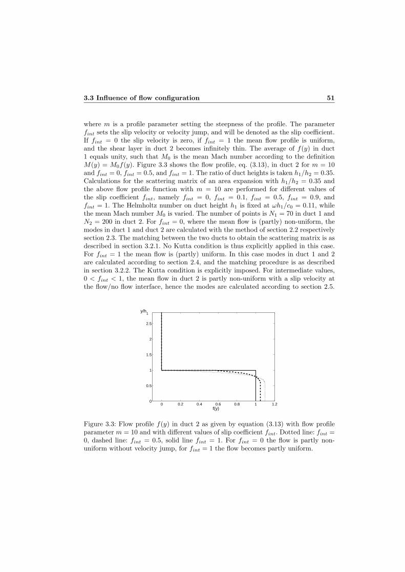
3.3 Influence of flow configuration 51
where m is a profile parameter setting the steepness of the profile. The parameterfint sets the slip velocity or velocity jump, and will be denoted as the slip coefficient.If fint = 0 the slip velocity is zero, if fint = 1 the mean flow profile is uniform,and the shear layer in duct 2 becomes infinitely thin. The average of f(y) in duct1 equals unity, such that M0 is the mean Mach number according to the definitionM(y) = M0f(y). Figure 3.3 shows the flow profile, eq. (3.13), in duct 2 for m = 10and fint = 0, fint = 0.5, and fint = 1. The ratio of duct heights is taken h1/h2 = 0.35.Calculations for the scattering matrix of an area expansion with h1/h2 = 0.35 andthe above flow profile function with m = 10 are performed for different values ofthe slip coefficient fint, namely fint = 0, fint = 0.1, fint = 0.5, fint = 0.9, andfint = 1. The Helmholtz number on duct height h1 is fixed at ωh1/c0 = 0.11, whilethe mean Mach number M0 is varied. The number of points is N1 = 70 in duct 1 andN2 = 200 in duct 2. For fint = 0, where the mean flow is (partly) non-uniform, themodes in duct 1 and duct 2 are calculated with the method of section 2.2 respectivelysection 2.3. The matching between the two ducts to obtain the scattering matrix is asdescribed in section 3.2.1. No Kutta condition is thus explicitly applied in this case.For fint = 1 the mean flow is (partly) uniform. In this case modes in duct 1 and 2are calculated according to section 2.4, and the matching procedure is as describedin section 3.2.2. The Kutta condition is explicitly imposed. For intermediate values,0 < fint < 1, the mean flow in duct 2 is partly non-uniform with a slip velocity atthe flow/no flow interface, hence the modes are calculated according to section 2.5.
0 0.2 0.4 0.6 0.8 1 1.20
0.5
1
1.5
2
2.5
f(y)
y/h1
Figure 3.3: Flow profile f(y) in duct 2 as given by equation (3.13) with flow profileparameter m = 10 and with different values of slip coefficient fint. Dotted line: fint =0, dashed line: fint = 0.5, solid line fint = 1. For fint = 0 the flow is partly non-uniform without velocity jump, for fint = 1 the flow becomes partly uniform.

52 Area expansion in a duct: modal analysis
Modes in duct 1 can be calculated as in section 2.2. Also for this case the Kuttacondition is applied in the matching between the two ducts, cf. section 3.2.2. Resultsfor the plane wave pressure reflection and transmission coefficients as function ofStrouhal number ωh1/U0, with U0 = M0c0, are shown in figures 3.4 through 3.7.The effect of going from a uniform flow profile to a non-uniform profile is here to
increase the magnitude of the reflection and transmission coefficients except for R−,of which the magnitude is decreased. Especially the magnitudes of the reflection andtransmission coefficients change smoothly as the flow profile is gradually changed.Results for fint = 0.1, giving a non-uniform flow with a small slip velocity in theshear layer, are nearly the same as those for fint = 0, where the slip velocity vanishes.This indicates that application of the Kutta condition in the first case does not have asignificant effect on the results compared to the latter case where the Kutta conditionis not imposed. Also for fint = 0.9 results are almost the same as for fint = 1.For fint = 0.9 neutral hydrodynamic modes are obtained, whereas in the fint = 1case, for which mean flow is uniform, they are absent. Therefore, it can be concludedthat any effect of the neutral hydrodynamic modes vanishes as the flow profile isgradually changed from non-uniform to uniform. Furthermore, the imaginary part ofthe wavenumber of the unstable hydrodynamic mode in duct 2 (i.e. the amplificationof the hydrodynamic instability) is shown in figure 3.8. For non-uniform flow withoutvelocity jump in the shear layer, fint = 0, the hydrodynamic instability vanishesabove a certain Strouhal number. This behaviour is typically found for physical shearlayers as discussed in appendix B.2 for the hyperbolic-tangent shear layer. For othervalues of fint hydrodynamic instability always occurs due to the velocity jump inthe shear layer. Consequently, for Strouhal number larger than about 3 the growthrate of the hydrodynamic instability found for fint = 0.1 begins to differ significantlyfrom that found for fint = 0. Nevertheless, the corresponding results for the reflectionand transmission coefficients, figures 3.4 through 3.7, are also practically the samefor these higher Strouhal numbers. The effect of the hydrodynamic instability, andin particular the non-vanishing of it, is thus negligible for high Strouhal numbers.This conclusion was also drawn by Boij and Nilsson [17] and Howe [44]. Moreover,for low and high Strouhal number especially the magnitudes of the reflection andtransmission coefficients converge to the same value for all values of fint, indicatinginsignificance of the mean flow profile in these limits.
3.3.2 Area expansion ratio
A striking feature is the hump in reflection and transmission found around Strouhalnumber equal to 1, cf. figures 3.4 through 3.7. For the values of fint equal to 0.5or less, the phase plots even suggest a sudden jump. This feature may be connectedto the behaviour of the hydrodynamic instability, since in the plot of hydrodynamicinstability growth rate, figure 3.8, also a hump is seen for all values of fint aroundthe same Strouhal number. It turns out that this is caused by the asymmetry in the

3.3 Influence of flow configuration 53
0 1 2 3 4 5 6 70.48
0.5
0.52
0.54
0.56
0.58
0.6
0.62
0.64
0.66
0.68
ω h1/U
0
|R+|
0 1 2 3 4 5 6 73.02
3.04
3.06
3.08
3.1
3.12
3.14
3.16
ω h1/U
0
arg(R+) (rad)
Figure 3.4: Magnitude and phase of the downstream plane wave pressure reflectioncoefficient R+ at an area expansion versus Strouhal number ωh1/U0 with ωh1/c0 =0.11, h1/h2 = 0.35, N1 = 70 and N2 = 200. Mean flow profile is given by eq.(3.13),where m = 10 and fint = 0 (×), fint = 0.1 (∗), fint = 0.5 (∇), fint = 0.9 (+) andfint = 1 (·) respectively. For fint = 0 no Kutta condition is applied in the modematching procedure, for other values of fint a Kutta condition is applied. Quasi-stationary solution without mean flow is: R+ = −0.4815.

54 Area expansion in a duct: modal analysis
0 1 2 3 4 5 6 70.52
0.53
0.54
0.55
0.56
0.57
0.58
0.59
0.6
ω h1/U
0
|T+|
0 1 2 3 4 5 6 7−0.035
−0.03
−0.025
−0.02
−0.015
−0.01
−0.005
0
ω h1/U
0
arg(T+) (rad)
Figure 3.5: Magnitude and phase of the downstream plane wave pressure transmissioncoefficient T+ at an area expansion versus Strouhal number ωh1/U0 with ωh1/c0 =0.11, h1/h2 = 0.35, N1 = 70 and N2 = 200. Mean flow profile is given by eq.(3.13),where m = 10 and fint = 0 (×), fint = 0.1 (∗), fint = 0.5 (∇), fint = 0.9 (+) andfint = 1 (·) respectively. For fint = 0 no Kutta condition is applied in the modematching procedure, for other values of fint a Kutta condition is applied. Quasi-stationary solution without mean flow is: T+ = 0.5185.

3.3 Influence of flow configuration 55
0 1 2 3 4 5 6 70.32
0.34
0.36
0.38
0.4
0.42
0.44
0.46
0.48
ω h1/U
0
|R−|
0 1 2 3 4 5 6 70
0.005
0.01
0.015
0.02
0.025
0.03
0.035
0.04
ω h1/U
0
arg(R−) (rad)
Figure 3.6: Magnitude and phase of the upstream plane wave pressure reflection coef-ficient R− at an area expansion versus Strouhal number ωh1/U0 with ωh1/c0 = 0.11,h1/h2 = 0.35, N1 = 70 and N2 = 200. Mean flow profile is given by eq.(3.13), wherem = 10 and fint = 0 (×), fint = 0.1 (∗), fint = 0.5 (∇), fint = 0.9 (+) and fint = 1(·) respectively. For fint = 0 no Kutta condition is applied in the mode matching pro-cedure, for other values of fint a Kutta condition is applied. Quasi-stationary solutionwithout mean flow is: R− = 0.4815.

56 Area expansion in a duct: modal analysis
0 1 2 3 4 5 6 71.45
1.5
1.55
1.6
1.65
1.7
1.75
1.8
1.85
ω h1/U
0
|T−|
0 1 2 3 4 5 6 7−0.06
−0.05
−0.04
−0.03
−0.02
−0.01
0
ω h1/U
0
arg(T−) (rad)
Figure 3.7: Magnitude and phase of the upstream plane wave pressure transmissioncoefficient T− at an area expansion versus Strouhal number ωh1/U0 with ωh1/c0 =0.11, h1/h2 = 0.35, N1 = 70 and N2 = 200. Mean flow profile is given by eq.(3.13),where m = 10 and fint = 0 (x), fint = 0.1 (∗), fint = 0.5 (∇), fint = 0.9 (+) andfint = 1 (.) respectively. For fint = 0 no Kutta condition is applied in the modematching procedure, for other values of fint a Kutta condition is applied. Quasi-stationary solution without mean flow is: T− = 1.4815.

3.3 Influence of flow configuration 57
0 1 2 3 4 5 6 70
100
200
300
400
500
ω h1/U
0
ℑ(khu
)/k0
Figure 3.8: Imaginary part of the wavenumber khu of the hydrodynamic instability(i.e growth rate) in duct 2 of the area expansion geometry scaled to k0 = ω/c0 versusStrouhal number ωh1/U0 for ωh1/c0 = 0.11. Mean flow profile is given by eq. (3.13),where m = 10 and fint = 0 (×), fint = 0.1 (∗), fint = 0.5 (∇), fint = 0.9 (+) andfint = 1 (·) respectively.
flow profile, i.e. the fact that in duct 2 of the expansion geometry the mean flow to nomean flow transition is not halfway the duct. This will be illustrated below for bothpartly uniform flow and partly non-uniform flow.
uniform flow
Figure 3.9 shows the imaginary part of the wavenumber of the unstable hydrodynamicmode as function of Strouhal number ωh1/U0 for different ratios of h1 and h2, obtainedby modal analysis calculations in case of partly uniform mean flow. As above, alsohere ω∗ = ωh1/c0 = 0.11. The number of points in the part with mean flow is fixedat N1 = 70, the total number of points N2 is thus determined by the ratio h1/h2.Indeed, the dependence of the (imaginary part of the) hydrodynamic wavenumber onthe Strouhal number strongly varies with h1/h2 ratio. For Strouhal numbers largerthan about 2 all results for h1/h2 ≤ 0.5 coincide. The results for h1/h2 = 0.7 onlycoincide with those for other h1/h2 ratios above a Strouhal number of approximately5.5.
The hydrodynamic instability is also calculated for the incompressible case. For

58 Area expansion in a duct: modal analysis
0 0.5 1 1.5 2 2.5 3 3.5 4 4.5 5 5.50
5
10
15
20
25
30
35
40
45
50
ω h1/U
0
ℑ(khu
)/k0
Figure 3.9: Imaginary part of the wavenumber khu of the hydrodynamic instability(i.e growth rate) in duct 2 of the area expansion geometry scaled to k0 = ω/c0 forpartly uniform mean flow as function of Strouhal number ωh1/U0. Modal analysiscalculations with ωh1/c0 = 0.11 and N1 = 70. h1/h2 ratios are h1/h2 = 0.175 (+),h1/h2 = 0.35 (×), h1/h2 = 0.5 (∗), and h1/h2 = 0.7 (∇).
partly uniform flow in a duct, giving an infinitely thin shear layer, the incompressiblesolution for the hydrodynamic instability modes was already given in section 2.7.2,in particular equations (2.38) and (2.40), in case the shear layer is halfway the duct.More generally, if the shear layer is at y = h1, as is considered in this chapter for duct2 downstream of the area expansion with 0 ≤ y ≤ h2 (figure 3.1), the incompressiblesolution is found in the same way:
Phu(y∗) =
⎧⎨⎩
A cosh(khu∗y∗) 0 ≤ y∗ ≤ 1,
B cosh(khu∗(y∗ − h2∗)) 1 ≤ y∗ ≤ h2∗.(3.14)
In this case h1 is used for non-dimensionalisation, thus h2∗ = h2/h1. A and B are coef-ficients determined by the wavenumber khu∗. The wavenumber is found by demandingcontinuity of pressure and displacement at y = h1, giving:
tanh(khu∗)(ω∗ −M0khu∗)2
=tanh(khu∗(1 − h2∗))
w2∗. (3.15)
This equation has to be solved numerically. The results obtained by modal analy-

3.3 Influence of flow configuration 59
0 0.5 1 1.5 2 2.5 30
5
10
15
20
25
30
ω h1/U
0
ℑ(khu
)/k0
Figure 3.10: Imaginary part of the wavenumber of the hydrodynamic instability (i.egrowth rate) in duct 2 of the area expansion geometry scaled to k0 = ω/c0 for partlyuniform mean flow as function of Strouhal number ωh1/U0. Modal analysis calcu-lations with ωh1/c0 = 0.11 and N1 = 70. h1/h2 ratios are h1/h2 = 0.35 (×) andh1/h2 = 0.5 (∗). Comparison with the incompressible solution is made: ◦ markers:h1/h2 = 0.35, solid line: h1/h2 = 0.5.
sis for ratios h1/h2 = 0.35 and h1/h2 = 0.5, cf. figure 3.9, are compared to theincompressible solution, equations (3.15) and (2.40) respectively, in figure 3.10. Theincompressible solutions for the hydrodynamic wavenumber are close to the resultsof the compressible modal analysis. This suggests that the observed behaviour of thehydrodynamic instability really is an effect related to the area expansion ratio h1/h2,regardless the presence of acoustic modes.
The magnitude and phase of the downstream plane wave pressure reflection coef-ficient R+ at the area expansion with uniform flow are shown in figure 3.11 for thedifferent h1/h2 ratios. The observed hump (i.e. local maximum) in the magnitudeand phase of the reflection coefficient for h1/h2 = 0.175 and h1/h2 = 0.35 seems tocoincide with the inflexion point in the plot of hydrodynamic instability growth rateversus Strouhal number, cf. figure 3.9. For the other h1/h2 ratios the dependenceof hydrodynamic instability growth rate as well as reflection coefficient on Strouhalnumber is more smooth.
A more elaborate picture of the influence of the area expansion ratio on the eigen-modes is given in figure 3.12. Here, the wavenumbers of the plane wave acoustic

60 Area expansion in a duct: modal analysis
0 0.5 1 1.5 2 2.5 3 3.5 4 4.5 50.1
0.2
0.3
0.4
0.5
0.6
0.7
0.8
0.9
ω h1/U
0
|R+|
0 0.5 1 1.5 2 2.5 3 3.5 4 4.5 52.9
2.95
3
3.05
3.1
3.15arg(R+) (rad)
ω h1/U
0
Figure 3.11: Magnitude and phase of the downstream plane wave pressure reflectioncoefficient R+ at an area expansion versus Strouhal number ωh1/U0 for (partly)uniform flow. Modal analysis calculation with ωh1/c0 = 0.11 and N1 = 70. Areaexpansion ratios are h1/h2 = 0.175 (+), h1/h2 = 0.35 (×), h1/h2 = 0.5 (∗), andh1/h2 = 0.7 (∇).

3.3 Influence of flow configuration 61
−10 −5 0 5 10 15 20
−60
−40
−20
0
20
40
60
ℜ(k)/k0
ℑ(k)/k0
hydrodynamic unstable
−x acoustic evanescent
+x acoustic evanescent
+x acoustic plane wave −x acoustic plane wave
(a) h1/h2 = 0.35
−10 −5 0 5 10 15 20
−80
−60
−40
−20
0
20
40
60
80
ℑ(k)/k0
ℜ(k)/k0
hydrodynamic unstable
−x acoustic evanescent
+x acoustic plane wave −x acoustic plane wave
+x acoustic evanescent
(b) h1/h2 = 0.5
Figure 3.12: Wavenumbers of the plane wave acoustic modes, the first six higherorder evanescent acoustic modes and the hydrodynamic instability modes for differentStrouhal numbers ωh1/U0 in case of an infinitely thin shear layer. Dimensionlessangular frequency and number of points in duct part with flow are fixed at ωh1/c0 =0.11 respectively N1 = 70. (a) ratio h1/h2 = 0.35, (b) ratio h1/h2 = 0.5. Strouhalnumbers are between 0.25 (× markers) and 2 (+ markers), wavenumbers for Strouhalnumber equal to 1 are indicated by the ∗ markers for all other values by the • markers.Note that for h1/h2 = 0.35 more points are taken in the vicinity of Strouhal= 1.

62 Area expansion in a duct: modal analysis
modes, the first six higher order evanescent acoustic modes in both directions and thehydrodynamic modes are shown for different Strouhal numbers for h1/h2 = 0.35 andh1/h2 = 0.5. Besides the influence of the expansion ratio on the hydrodynamic modes,discussed above, also the acoustic modes are strongly affected by the expansion ratio.Moving from h1/h2 = 0.5 to h1/h2 = 0.35 the imaginary part of the wavenumberof the evanescent acoustic modes decreases, which means they are less damped. Alsofor some evanescent acoustic modes the real part of the wavenumber (related to thethe phase velocity) becomes significant. A clear maximum in the real part of thewavenumber of the first evanescent acoustic mode is seen around a Strouhal numberof 1.
non-uniform flow
Similarly, the jump seen in the reflection and transmission coefficients for non-uniformflow, cf. figures 3.4 through 3.7, is connected to the behaviour of the modes’ wavenum-bers as function of the area expansion ratio. For the flow profile, given by equation(3.13), with fint = 0 (no velocity jump in the shear layer) and m = 10, the wavenum-bers of the modes in downstream duct 2 for several Strouhal numbers ωh1/U0 areshown in figure 3.13 for expansion ratios h1/h2 = 0.35 and h1/h2 = 0.5. For Strouhalnumber around 1 the wavenumbers of the first higher order evanescent acoustic modesand the hydrodynamic instability modes are very close for the h1/h2 = 0.35 case com-pared to the h1/h2 = 0.5 case. At first sight the traces of the wavenumbers as functionof Strouhal number for these modes seem to be well distinguishable for h1/h2 = 0.35.However, for low Strouhal number the wavenumber of the hydrodynamic instabil-ity mode is expected to tend to zero, while for higher Strouhal number at least thereal part of the wavenumber is expected to be large compared to the wavenumberof the first higher order evanescent acoustic mode. This would be in contradictionwith the two supposed traces of the wavenumbers of these modes. Causality analy-sis for the modes, cf. section 2.6, indicates that indeed a ’jump’ occurs between thefirst higher order evanescent acoustic mode and the hydrodynamic unstable modeat a certain Strouhal number. Remarkably, according to the Briggs-Bers formalismthe jump accors between Strouhal number ωh1/U0 = 1.047 and ωh1/U0 = 1.048,whereas the Crighton-Leppington formalism indicates the jump between Strouhalnumber ωh1/U0 = 1.048 and ωh1/U0 = 1.049, see figures 3.14 and 3.15 respectively.The traces entering the pictures from the right originate in the lower complex plane,while the traces entering from the left originate in the upper complex plane. Thisleads to the given classification of the modes. The pressure disturbance P (y) of thetwo modes is shown in figure 3.16 for Strouhal number 1.047. For Strouhal numbers1.048 and 1.049, where the jump from hydrodynamic unstable to acoustic evanescentand vice versa has occured (depending on causality criterium formalism), the modesstay virtually the same. Clearly, the two modes are very similar, and a distinction onbasis of their shape could not readily be made.

3.3 Influence of flow configuration 63
−10 −5 0 5 10 15 20 25
−60
−40
−20
0
20
40
60
ℜ(k)/k0
ℑ(k)/k0
−x acoustic plane wave
+x acoustic plane wave
−x acoustic evanescent
+x acoustic evanescent
hydrodynamic neutral
hydrodynamic unstable/ −x acoustic evanescent
(a) h1/h2 = 0.35
−10 −5 0 5 10 15 20 25
−80
−60
−40
−20
0
20
40
60
80
ℜ(k)/k0
ℑ(k)/k0
+x acoustic plane wave
−x acoustic plane wave
−x acoustic evanescent
hydrodynamic unstable
hydrodynamic neutral
+x acoustic evanescent
(b) h1/h2 = 0.5
Figure 3.13: Wavenumbers of the plane wave acoustic modes, the first six higherorder evanescent acoustic modes, hydrodynamic instability modes and neutral hydro-dynamic modes for different Strouhal numbers ωh1/U0 in case of partly non-uniformflow. Flow profile is as given by equation (3.13) with fint = 0 and m = 10. Dimen-sionless angular frequency and number of points in duct part with flow are fixed atωh1/c0 = 0.11 respectively N1 = 70. (a) ratio h1/h2 = 0.35, (b) ratio h1/h2 = 0.5.Strouhal numbers are between 0.25 (× markers) and 2 (+ markers), wavenumbers forStrouhal number equal to 1 are indicated by the ∗ markers, and for all other valuesby the · markers. Note that for h1/h2 = 0.35 more points are taken in the vicinity ofStrouhal= 1.
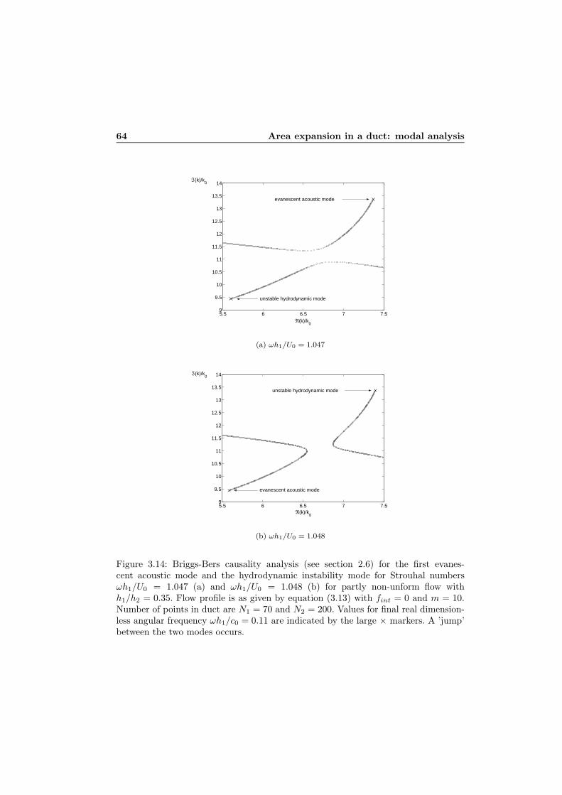
64 Area expansion in a duct: modal analysis
5.5 6 6.5 7 7.59
9.5
10
10.5
11
11.5
12
12.5
13
13.5
14ℑ(k)/k
0
ℜ(k)/k0
unstable hydrodynamic mode
evanescent acoustic mode
(a) ωh1/U0 = 1.047
5.5 6 6.5 7 7.59
9.5
10
10.5
11
11.5
12
12.5
13
13.5
14
unstable hydrodynamic mode
evanescent acoustic mode
ℜ(k)/k0
ℑ(k)/k0
(b) ωh1/U0 = 1.048
Figure 3.14: Briggs-Bers causality analysis (see section 2.6) for the first evanes-cent acoustic mode and the hydrodynamic instability mode for Strouhal numbersωh1/U0 = 1.047 (a) and ωh1/U0 = 1.048 (b) for partly non-unform flow withh1/h2 = 0.35. Flow profile is as given by equation (3.13) with fint = 0 and m = 10.Number of points in duct are N1 = 70 and N2 = 200. Values for final real dimension-less angular frequency ωh1/c0 = 0.11 are indicated by the large × markers. A ’jump’between the two modes occurs.

3.3 Influence of flow configuration 65
5.5 6 6.5 7 7.59
9.5
10
10.5
11
11.5
12
12.5
13
13.5
14
ℜ(k)/k0
ℑ(k)/k0
unstable hydrodynamic mode
evanescent acoustic mode
(a) ωh1/U0 = 1.048
5.5 6 6.5 7 7.59
9.5
10
10.5
11
11.5
12
12.5
13
13.5
14
unstable hydrodynamic mode
evanescent acoustic mode
ℜ(k)/k0
ℑ(k)/k0
(b) ωh1/U0 = 1.049
Figure 3.15: Crighton-Leppington causality analysis (see section 2.6) for the firstevanescent acoustic mode and the hydrodynamic instability mode for Strouhal num-bers ωh1/U0 = 1.048 (a) and ωh1/U0 = 1.049 (b) for partly non-unform flow withh1/h2 = 0.35. Flow profile is as given by equation (3.13) with fint = 0 and m = 10.Number of points in duct are N1 = 70 and N2 = 200. Values for final real dimension-less angular frequency ωh1/c0 = 0.11 are indicated by the large × markers. A ’jump’between the two modes occurs.

66 Area expansion in a duct: modal analysis
0 0.5 1 1.5 2 2.5 3 0.2
0.3
0.4
0.5
0.6
0.7
0.8
0.9
1|P|
y/h1
0 0.5 1 1.5 2 2.5 3 −2
−1.5
−1
−0.5
0
0.5
1
1.5
y/h1
arg(P) (rad)
Figure 3.16: Absolute value and phase for the pressure disturbance P (y) of the twomodes with wavenumber k/k0 ≈ 5.60 + 9.44i (dashed line) and k/k0 = 7.37 + 13.37i(solid line), which jump from hydrodynamic unstable to acoustic evenescent and viceversa. Absolute value and phase at the first discrete point are scaled to unity re-spectively set at zero. Strouhal number is ωh1/U0 = 1.047, dimensionless angularfrequency ωh1/c0 = 0.11. For Strouhal numbers 1.048 and 1.049 the modes are virtu-ally the same. Flow profile is as given by equation (3.13) with fint = 0 and m = 10.Number of points in duct are N1 = 70 and N2 = 200.

3.4 Cartesian and cylindrical geometry 67
The jump between acoustic evanescent and hydrodynamic unstable mode coin-cides with the jump in reflection and transmission coefficients, which occurs at thesame Strouhal number, already seen in figures 3.4 through 3.7. The result for thedownstream reflection coefficient R+ for expansion ratio h1/h2 = 0.35 is again shownin figure 3.17 together with the result for h1/h2 = 0.5. The Crighton-Leppingtoncausality analysis is utilized, giving a jump in both magnitude and phase of the re-flection coefficient between Strouhal number ωh1/U0 = 1.048 and ωh1/U0 = 1.049.Using the Briggs-Bers causality analysis gives the same results, only the jump occursbetween ωh1/U0 = 1.047 and ωh1/U0 = 1.048. For expansion ratio h1/h2 = 0.5 nojump occurs between the first acoustic evanescent and hydrodynamic unstable mode,and consequently no jump in reflection coefficient is observed, although a hump canbe seen in the phase of the reflection coefficient around Strouhal number 1. This wasalso seen for an infinitely thin shear layer at the same expansion ratio, cf. figure 3.11.
3.4 Cartesian and cylindrical geometry
Boij and Nilsson [16, 17] presented a model for scattering at an area expansion in atwo-dimensional rectangular duct. They proposed a scaling between two-dimensionalrectangular and two-dimensional cylindrical geometry, such that comparison withexperimental data of Ronneberger [97, 100], obtained for an expansion in a cylindricalduct, could be made. In this section modal analysis calculations for an area expansionin both two-dimensional rectangular and two-dimensional cylindrical geometry willbe compared, in order to test the proposed scaling.
3.4.1 Scaling of the Helmholtz number
In order to compare their theoretical predictions for an expansion in a two-dimensionalrectangular duct with the experimental data of Ronneberger [97, 100] for an expansionin a cylindrical duct, Boij and Nilsson [16, 17] proposed a scaling of the Helmholtznumber. For low frequencies well below the cut-on of the first higher order acousticmode, only a plane wave is incident on the area expansion. For cylindrical geometrythe incident sound pressure field is thus independent of the angular coordinate, andconsequently higher order modes which are only dependent on the radial coordinate(radial modes) will be excited at the expansion. From this they reasoned that thearea expansion in a cylindrical duct can be considered to be a two-dimensional prob-lem, and hence can be related to their theory for a two-dimensional rectangular duct.Furthermore, they argued that the predominant feature is the onset of higher ordermodes in the large duct downstream of the expansion. For low frequency the wave-length is much larger than the transverse dimension of the duct, such that geometricaldetails will not be resolved by the sound field. The plane wave scattering at the areaexpansion would therefore be reasonably similar for a rectangular and a cylindrical

68 Area expansion in a duct: modal analysis
0 1 2 3 4 5 6 70.3
0.35
0.4
0.45
0.5
0.55
0.6
0.65
0.7
0.75|R+|
ω h1/U
0
0 1 2 3 4 5 6 73.02
3.04
3.06
3.08
3.1
3.12
3.14
arg(R+) (rad)
ω h1/U
0
Figure 3.17: Magnitude and phase of the downstream plane wave pressure reflectioncoefficient R+ at an area expansion against Strouhal number ωh1/U0 for partly non-uniform flow. Flow profile is as given by equation (3.13) with fint = 0 and m = 10.Modal analysis calculation with ωh1/c0 = 0.11 and N1 = 70. Area expansion ratiosare h1/h2 = 0.35 (×) and h1/h2 = 0.5 (∗).
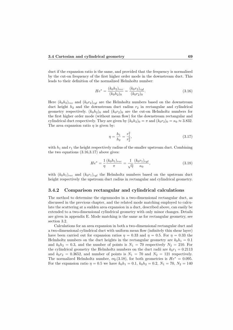
3.4 Cartesian and cylindrical geometry 69
duct if the expansion ratio is the same, and provided that the frequency is normalisedby the cut-on frequency of the first higher order mode in the downstream duct. Thisleads to their definition of the normalized Helmholtz number:
He∗ =(k0h2)rec
(k0h2)0=
(k0r2)cyl
(k0r2)0. (3.16)
Here (k0h2)rec and (k0r2)cyl are the Helmholtz numbers based on the downstreamduct height h2 and the downstream duct radius r2 in rectangular and cylindricalgeometry respectively. (k0h2)0 and (k0r2)0 are the cut-on Helmholtz numbers forthe first higher order mode (without mean flow) for the downstream rectangular andcylindrical duct respectively. They are given by (k0h2)0 = π and (k0r2)0 = κ0 ≈ 3.832.The area expansion ratio η is given by:
η =h1
h2=r21r22, (3.17)
with h1 and r1 the height respectively radius of the smaller upstream duct. Combiningthe two equations (3.16,3.17) above gives:
He∗ =1η
(k0h1)rec
π=
1√η
(k0r1)cyl
κ0, (3.18)
with (k0h1)rec and (k0r1)cyl the Helmholtz numbers based on the upstream ductheight respectively the upstream duct radius in rectangular and cylindrical geometry.
3.4.2 Comparison rectangular and cylindrical calculations
The method to determine the eigenmodes in a two-dimensional rectangular duct, asdiscussed in the previous chapter, and the related mode matching employed to calcu-late the scattering at a sudden area expansion in a duct, described above, can easily beextended to a two-dimensional cylindrical geometry with only minor changes. Detailsare given in appendix E. Mode matching is the same as for rectangular geometry, seesection 3.2.
Calculations for an area expansion in both a two-dimensional rectangular duct anda two-dimensional cylindrical duct with uniform mean flow (infinitely thin shear layer)have been carried out for expansion ratios η = 0.33 and η = 0.5. For η = 0.33 theHelmholtz numbers on the duct heights in the rectangular geometry are k0h1 = 0.1and k0h2 = 0.3, and the number of points is N1 = 70 respectively N2 = 210. Forthe cylindrical geometry the Helmholtz numbers on the duct radii are k0r1 = 0.2113and k0r2 = 0.3652, and number of points is N1 = 70 and N2 = 121 respectively.The normalized Helmholtz number, eq.(3.18), for both geometries is He∗ = 0.095.For the expansion ratio η = 0.5 we have k0h1 = 0.1, k0h2 = 0.2, N1 = 70, N2 = 140

70 Area expansion in a duct: modal analysis
for rectangular geometry and k0r1 = 0.1725, k0r2 = 0.2440, N1 = 70 and N2 = 99for cylindrical geometry. Normalized Helmholtz number is He∗ = 0.064. Figure 3.18shows the absolute values of the reflection and transmission coefficients versus Machnumber M for the two area expansion ratios for both rectangular and cylindricalgeometry. The relative deviation in absolute value of the reflection and transmissioncoefficients between the rectangular and cylindrical calculations is given in figure 3.19for both expansion ratios. The relative deviation is defined as:
∣∣∣ |R+|rec − |R+|cyl
|R+|rec
∣∣∣,etcetera. Generally, for both expansion ratios the results of the rectangular and cylin-drical calculations are reasonably close, cf. figure 3.18. Around Mach numberM = 0.1,corresponding to a Strouhal number ωh1/U0 = 1, a hump in reflection and transmis-sion coefficients is seen, especially for |R+| and |T−|, for the rectangular calculationswith expansion ratio η = 0.33. This feature is an effect of the area expansion ratioh1/h2, as discussed above section 3.3.2. However, in the cylindrical calculations it isnot observed (as strongly). This results in a relatively large deviation, especially for|R+| and |T−|, around Mach number M = 0.1, cf. figure 3.19. Also, for expansionratio η = 0.5 an increased relative deviation is found around Mach number M = 0.1,although it is about 5 times smaller than for η = 0.33. The relative deviation inthe magnitude of the upstream reflection and transmission coefficients, R− and T−,increases with mean flow velocity for higher Mach numbers, whereas for the down-stream reflection and transmission coefficients, R+ and T+ the deviation in magnituderemains relatively small.
3.4.3 Influence of ratio of duct radii
For equal area expansion ratio, η = h1/h2 = r21/r22, results for reflection and trans-
mission coefficients display a deviation when calculated for rectangular or cylindricalgeometry, cf. figure 3.18 and 3.19. Specifically a hump in R+ and T− is seen arounda Strouhal number of 1 for the rectangular geometry. Figure 3.11 indicates that thisfeature only occurs for ratios h1/h2 less than 0.5. In comparing the rectangular andcylindrical geometry calculations, figure 3.18 and 3.19, the lowest value for the ex-pansion ratio is η = 0.33. This yields a ratio of duct heights in rectangular geometryof h1/h2 = 0.33 and a much larger ratio of duct radii in cylindrical geometry ofr1/r2 = 0.57. The behaviour of reflection and transmission coefficients for some otherdifferent ratios of r1/r2 is shown in figure 3.20 in case of uniform mean flow. As forrectangular geometry with ratio of duct heights h1/h2 less than 0.5, cf.figure 3.18, ahump in the magnitude of downstream reflection coefficient R+ and upstream trans-mission coefficient T− is seen around Mach number M = 0.05 for ratio of radii r1/r2less than 0.5. This feature, which is connected to the behaviour of the modes in section

3.4 Cartesian and cylindrical geometry 71
0 0.05 0.1 0.15 0.2 0.25 0.3 0.35 0.4 0.45 0.5
0.35
0.4
0.45
0.5
0.55
0.6
0.65
0.7
0.75
M
|R+|
η=0.33
η=0.5
0 0.05 0.1 0.15 0.2 0.25 0.3 0.35 0.4 0.45 0.50.5
0.55
0.6
0.65
0.7
0.75
M
|T+|
η=0.33
η=0.5
0 0.05 0.1 0.15 0.2 0.25 0.3 0.35 0.4 0.45 0.50.2
0.25
0.3
0.35
0.4
0.45
0.5
M
|R−|
η=0.33
η=0.5
0 0.05 0.1 0.15 0.2 0.25 0.3 0.35 0.4 0.45 0.51.3
1.4
1.5
1.6
1.7
1.8
M
|T−|
η=0.5
η=0.33
Figure 3.18: Absolute values of the reflection and transmission coefficients versus MachnumberM for rectangular geometry (+ markers) and cylindrical geometry (◦ markers)for two area expansion ratios η in case of an infinitely thin shear layer. For η = 0.33:He∗ = 0.095, k0h1 = 0.1, k0h2 = 0.3, k0r1 = 0.2113, k0r2 = 0.3652, N1 = 70, andN2 = 210 respectively N2 = 121 for rectangular and cylindrical geometry. For η = 0.5:He∗ = 0.064, k0h1 = 0.1, k0h2 = 0.2, k0r1 = 0.1725, k0r2 = 0.2440, N1 = 70, andN2 = 140 respectively N2 = 99 for rectangular and cylindrical geometry.

72 Area expansion in a duct: modal analysis
0 0.1 0.2 0.3 0.4 0.50
0.005
0.01
0.015
0.02
0.025
0.03
rela
tive
devi
atio
n
M
(a) η = 0.33
0 0.1 0.2 0.3 0.4 0.50
1
2
3
4
5
6
7
8x 10
−3
M
rela
tive
devi
atio
n
(b) η = 0.5
Figure 3.19: Relative deviation in |R+| (+ markers), |T+| (∗ markers), |R−| (∇ mark-ers) and |T−| (◦ markers) when comparing calculations for rectangular and cylindricalgeometry, cf. figure 3.18, for expansion ratio η = 0.33 (a) and η = 0.5 (b).
3.3.2, thus depends in the same manner on the ratio of duct heights for rectangulargeometry respectively duct radii for cylindrical geometry.
3.5 Comparison with an alternative model and ex-perimental data
Boij and Nilsson [16, 17] presented a model for scattering at an area expansion in atwo-dimensional rectangular duct with uniform mean flow based on the Wiener-Hopftechnique. Results were compared to experimental data of Ronneberger [97, 100] fora cylindrical pipe using the Helmholtz scaling discussed above in section 3.4.1. In theexperiments of Ronneberger the pipe radius upstream of the expansion is r1 = 25mm, the pipe radius downstream of the expansion is r2 = 42.5 mm. This yields anarea expansion ratio of η = 0.35. Measurements are done at various frequencies andMach numbers. Here, we will compare with the experiments, and corresponding modelcalculations of Boij and Nilsson, for which the frequency is f = 500 Hz. This givesa Helmholtz number on the upstream duct radius of k0r1 = 0.227 and a normalizedHelmholtz number He∗ = 0.10. For the rectangular geometry this yields a Helmholtznumber on the upstream duct height of k0h1 = 0.11.
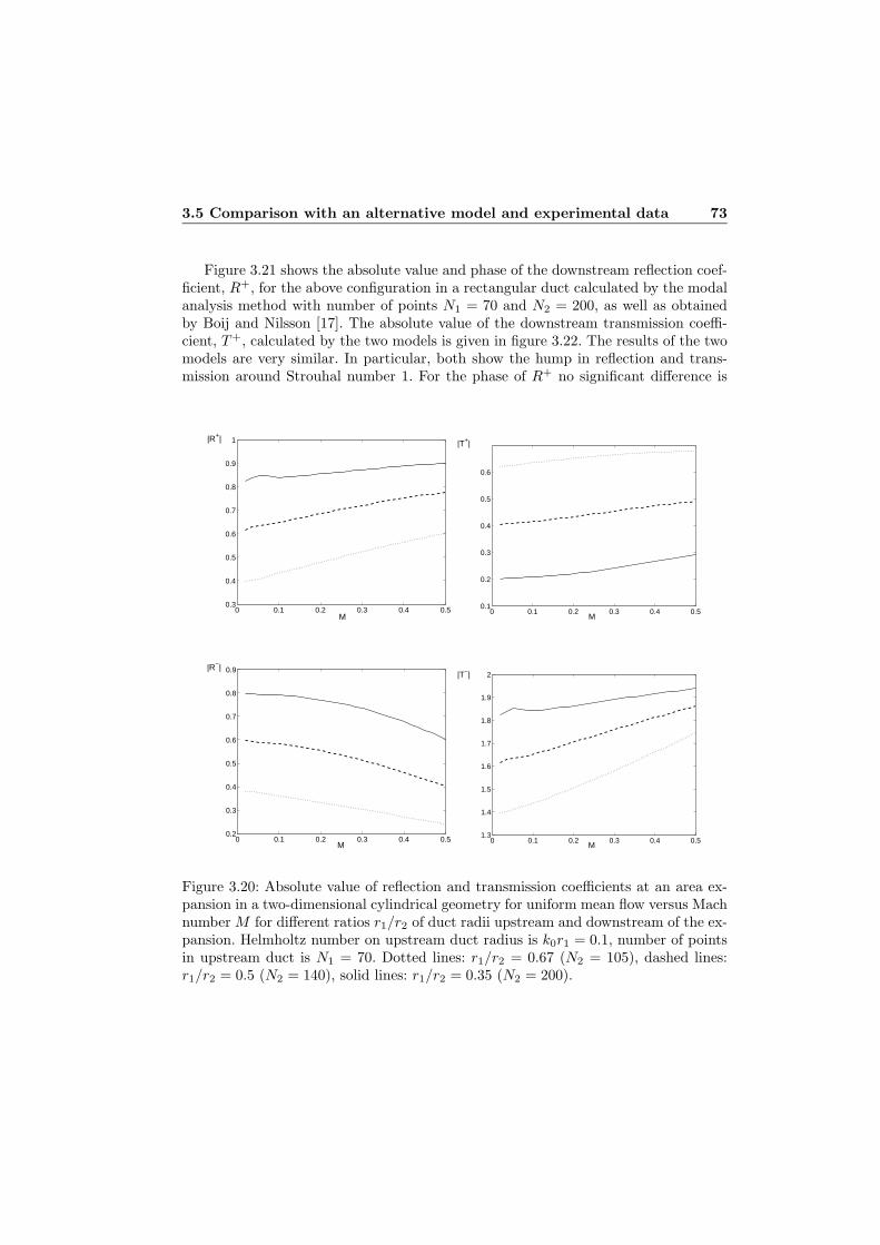
3.5 Comparison with an alternative model and experimental data 73
Figure 3.21 shows the absolute value and phase of the downstream reflection coef-ficient, R+, for the above configuration in a rectangular duct calculated by the modalanalysis method with number of points N1 = 70 and N2 = 200, as well as obtainedby Boij and Nilsson [17]. The absolute value of the downstream transmission coeffi-cient, T+, calculated by the two models is given in figure 3.22. The results of the twomodels are very similar. In particular, both show the hump in reflection and trans-mission around Strouhal number 1. For the phase of R+ no significant difference is
0 0.1 0.2 0.3 0.4 0.50.3
0.4
0.5
0.6
0.7
0.8
0.9
1|R+|
M0 0.1 0.2 0.3 0.4 0.5
0.1
0.2
0.3
0.4
0.5
0.6
|T+|
M
0 0.1 0.2 0.3 0.4 0.50.2
0.3
0.4
0.5
0.6
0.7
0.8
0.9|R−|
M0 0.1 0.2 0.3 0.4 0.5
1.3
1.4
1.5
1.6
1.7
1.8
1.9
2|T−|
M
Figure 3.20: Absolute value of reflection and transmission coefficients at an area ex-pansion in a two-dimensional cylindrical geometry for uniform mean flow versus Machnumber M for different ratios r1/r2 of duct radii upstream and downstream of the ex-pansion. Helmholtz number on upstream duct radius is k0r1 = 0.1, number of pointsin upstream duct is N1 = 70. Dotted lines: r1/r2 = 0.67 (N2 = 105), dashed lines:r1/r2 = 0.5 (N2 = 140), solid lines: r1/r2 = 0.35 (N2 = 200).

74 Area expansion in a duct: modal analysis
0 1 2 3 4 5 6 7
0.5
0.55
0.6
0.65
0.7
|R+|
ω h1/U
0
0 1 2 3 4 5 6 73.03
3.04
3.05
3.06
3.07
3.08
ω h1/U
0
arg(R+) (rad)
Figure 3.21: Magnitude and phase of the downstream reflection coefficient R+ atan area expansion in a two-dimensional rectangular duct with uniform flow versusStrouhal number. Helmholtz number on upstream duct height: k0h1 = 0.11, areaexpansion ratio: η = h1/h2 = 0.35, normalized Helmholtz number: He∗ = 0.10.Solid lines: results of modal analysis method (N1 = 70, N2 = 200). Dotted lines:fit of Boij and Nilsson’s result [16, 17]. Quasi-stationary limit without mean flow is:R+ = −0.4815.

3.5 Comparison with an alternative model and experimental data 75
0 1 2 3 4 5 6 70.5
0.52
0.54
0.56
0.58
0.6
0.62|T+|
ω h1/U
0
Figure 3.22: Absolute value of the downstream transmission coefficient T+ at an areaexpansion in a two-dimensional rectangular duct with uniform flow versus Strouhalnumber. Helmholtz number on upstream duct height: k0h1 = 0.11, area expansionratio: η = h1/h2 = 0.35, normalized Helmholtz number: He∗ = 0.10. Solid lines:results of modal analysis method (N1 = 70, N2 = 200). Dotted lines: fit of Boij andNilsson’s result [17]. Quasi-stationary limit without mean flow is: T+ = 0.5185.
seen between the two models (The difference seen in the graph is due to the error inextracting the data from reference [16]). Nevertheless, a deviation in the results for theabsolute values is seen. Generally, the mode matching method gives a lower absolutevalue for the reflection coefficient and a higher one for the transmission coefficientthan Boij and Nilsson’s model. For the absolute value of the reflection coefficient thedeviation between the two models is fairly constant at about 1%, at least above aStrouhal number of ∼ 0.5. The absolute value of the transmission coefficient displaysa larger deviation, it increases from about 1% for low Strouhal number to about 4%for high Strouhal number.
In comparing model results with experimental data, particularly the effect of intro-ducing a non-uniform mean flow will be investigated. The flow profile in the upstreamtube in Ronneberger’s experiments can be assumed to obey the empirical power lawfor turbulent pipe flow as given by Schlichting [102], such that we have:
f(r) =
⎧⎪⎨⎪⎩
(2m+1)(m+1)2m2
(1 − r
r1
) 1m
0 ≤ y ≤ r1,
0 r1 < y ≤ r2
. (3.19)
76 Area expansion in a duct: modal analysis
The value of the profile function f(r) averaged over the upstream pipe area πr21 equalsunity. the Mach number as function of radius is given by: M(r) = M0f(r), such thatM0 is the area averaged Mach number in the upstream pipe. The profile parameterm varies with Reynolds number Re on the pipe diameter and the average mean flowvelocity:
Re =2r1U0
ν, (3.20)
with U0 = M0c0 and ν the kinematic viscosity. For air at room temperature andatmospheric pressure ν = 1.5·10−5 m2s−1. Values form at different Reynolds numbersare given in table 3.1. For the measurements with mean flow the Mach numbers are inthe range of M0 ≈ 0.018 to M0 ≈ 0.45. The upstream pipe radius is r1 = 2.5 ·10−2 m.This gives values for the Reynolds number in the range Re ≈ 2.1·104 to Re ≈ 5.1·105.Consequently, the profile parameter will be between m ≈ 6.5 for low Mach numberand m ≈ 7.7 for high Mach number. Besides this turbulent profile we consider theprofile given by equation (3.13) for rectangular geometry. For cylindrical geometry itis given by:
f(r) =
⎧⎨⎩
m+2m (1 − ( r
r1)m) 0 ≤ y ≤ r1
0 r1 < y ≤ r2
(3.21)
Also here the average of the profile function over the upstream pipe area equals unity.This profile is close to laminar. Figures 3.23 through 3.26 show the experimental dataof Ronneberger [100] for the downstream and upstream reflection and transmissioncoefficients at the area expansion with the above given configuration. The results areplotted versus the Strouhal number based on the equivalent upstream duct heighth1 in rectangular geometry. On basis of the representation of the data in reference[100], the error in the magnitudes and phases is estimated at ±0.01 and ±0.04 (≈±0.01π) respectively. The figures also show results of mode matching calculationsfor cylindrical geometry with uniform mean flow as well as with the turbulent flowprofile, eq.(3.19), with m = 7, and the flow profile of eq.(3.21) with m = 15. Theselatter two non-uniform profiles are plotted in figure 3.27. The number of points in themode matching calculations is N1 = 118 and N2 = 200. If applicable, also the resultsof Boij and Nilsson are given. The effect of a non-uniform mean flow compared touniform mean flow on the magnitude of the reflection and transmission coefficients inthe mode matching method is opposite for the turbulent pipe flow and the alternative
Table 3.1: Values of profile parameter m for the turbulent pipe flow profile, equation(3.19), as function of Reynolds number Re, given by Schlichting [102].Re 4 · 103 2.3 · 104 1.1 · 105 1.1 · 106 2.0 · 106 3.2 · 106
m 6.0 6.6 7.0 8.8 10 10

3.5 Comparison with an alternative model and experimental data 77
0 1 2 3 4 5 6 70.45
0.5
0.55
0.6
0.65
0.7
0.75|R+|
ω h1/U
0
0 1 2 3 4 5 6 73
3.05
3.1
3.15arg(R+)(rad)
ω h1/U
0
Figure 3.23: Magnitude and phase of downstream reflection coefficient R+ at an areaexpansion. Helmholtz number on upstream duct radius: k0r1 = 0.227, expansion ra-tio: η = 0.35, normalized Helmholtz number: He∗ = 0.10. On the horizontal axis isthe Strouhal number based on the equivalent upstream duct height h1 in rectangulargeometry. ∗ markers: experimental data Ronneberger [100]. Mode matching calcula-tions in cylindrical geometry (N1 = 118, N2 = 200) for: uniform mean flow (solid line),turbulent pipe flow, eq. (3.19), with m = 7 (dashed line), and flow profile eq.(3.21)with m = 15 (dotted line). Solid line with • markers: fit of Boij and Nilsson’s result[16, 17]. Quasi-stationary limit without mean flow is: R+ = −0.4815.

78 Area expansion in a duct: modal analysis
0 1 2 3 4 5 6 70.5
0.51
0.52
0.53
0.54
0.55
0.56
0.57
0.58
0.59
0.6|T+|
ω h1/U
0
0 1 2 3 4 5 6 7−0.04
−0.02
0
0.02
0.04
0.06
0.08
0.1arg(T+)(rad)
ω h1/U
0
Figure 3.24: Magnitude and phase of downstream transmission coefficient T+ at anarea expansion. Helmholtz number on upstream duct radius: k0r1 = 0.227, expan-sion ration: η = 0.35, normalized Helmholtz number: He∗ = 0.10. On the horizontalaxis is the Strouhal number based on the equivalent upstream duct height h1 in rect-angular geometry. ∗ markers: experimental data Ronneberger [100]. Mode matchingcalculations in cylindrical geometry (N1 = 118, N2 = 200) for: uniform mean flow(solid line), turbulent pipe flow, eq. (3.19), with m = 7 (dashed line), and flow profileeq.(3.21) with m = 15 (dotted line). Solid line with • markers: fit of Boij and Nilsson’sresult [17]. Quasi-stationary limit without mean flow is: T+ = 0.5185.

3.5 Comparison with an alternative model and experimental data 79
0 1 2 3 4 5 6 70.25
0.3
0.35
0.4
0.45
0.5|R−|
ω h1/U
0
0 1 2 3 4 5 6 70
0.05
0.1
0.15
0.2
0.25
0.3arg(R−)(rad)
ω h1/U
0
Figure 3.25: Magnitude and phase of upstream reflection coefficient R− at an area ex-pansion. Helmholtz number on upstream duct radius: k0r1 = 0.227, expansion ration:η = 0.35, normalized Helmholtz number: He∗ = 0.10. On the horizontal axis is theStrouhal number based on the equivalent upstream duct height h1 in rectangular ge-ometry. ∗ markers: experimental data Ronneberger [100]. Mode matching calculationsin cylindrical geometry (N1 = 118, N2 = 200) for: uniform mean flow (solid line), tur-bulent pipe flow, eq.(3.19), with m = 7 (dashed line), and flow profile eq.(3.21) withm = 15 (dotted line). Quasi-stationary limit without mean flow is: R− = 0.4815.

80 Area expansion in a duct: modal analysis
0 1 2 3 4 5 6 71.45
1.5
1.55
1.6
1.65
1.7
1.75
1.8
1.85
1.9
ω h1/U
0
|T−|
0 1 2 3 4 5 6 7−0.1
−0.08
−0.06
−0.04
−0.02
0
0.02
0.04arg(T−)(rad)
ω h1/U
0
Figure 3.26: Magnitude and phase of upstream transmission coefficient T− at an areaexpansion. Helmholtz number on upstream duct radius: k0r1 = 0.227, expansion ra-tion: η = 0.35, normalized Helmholtz number: He∗ = 0.10. On the horizontal axis isthe Strouhal number based on the equivalent upstream duct height h1 in rectangulargeometry. ∗ markers: experimental data Ronneberger [100]. Mode matching calcula-tions in cylindrical geometry (N1 = 118, N2 = 200) for: uniform mean flow (solid line),turbulent pipe flow, eq.(3.19), with m = 7 (dashed line), and flow profile eq.(3.21)with m = 15 (dotted line). Quasi-stationary limit without mean flow is: T− = 1.4815.

3.5 Comparison with an alternative model and experimental data 81
0 0.2 0.4 0.6 0.8 1 1.2 1.40
0.2
0.4
0.6
0.8
1.0
1.2
1.4
1.6
1.8
f(r)
r/r1
Figure 3.27: Non-uniform flow profiles as used in the mode matching calculations,figures 3.23 through 3.26. Dashed line: turbulent pipe flow, equation (3.19), withparameter m = 7. Dotted line: flow profile function, equation (3.21), with m = 15.
profile. The magnitudes of R+, T+ and T− decrease when taking the turbulent profilecompared to the uniform flow profile, whereas the magnitude of R− increases. Forthe alternative non-uniform profile this is exactly opposite. Concerning the phase ofthe reflection and transmission coefficients the turbulent profile and the alternativenon-uniform profile qualitatively have the same effect compared to uniform flow forR+ and T−. For the phase of T+ and R− the effect is opposite. The flow profilewhich gives the best fit between mode matching calculations and experimental datavaries for the different reflection and transmission coefficients. For the magnitudeof R+ the alternative non-uniform profile clearly gives a better resemblance withexperimental data compared to the uniform profile, whereas the turbulent profile givesa worse prediction. For the phase of R+ the alternative profile seems to give betterresults for some Strouhal numbers, however the turbulent profile gives the best resultsfor very low Strouhal. The experimental data for the magnitude of the downstreamtransmission coefficient T+ is between the mode matching results for uniform flowand turbulent pipe flow. The alternative profile gives worse resemblance comparedto uniform flow. The same as for T+ is more or less seen for the upstream reflectioncoefficient R−. Although here, clearly, the turbulent profile gives better resemblancewith experiments for the magnitude of R− at Strouhal numbers larger than 1. Thealternative profile gives a worse prediction for both magnitude and phase of R−. Forthe upstream transmission coefficient T− the results for the alternative non-uniform

82 Area expansion in a duct: modal analysis
flow profile are most consistent with experimental data, both for magnitude andphase. The turbulent profile gives a worse prediction at least for the magnitude of T−
compared to the other profiles.In short, for the magnitudes of R+ and T− the calculations with the alternative
non-uniform flow profile give a better prediction than those with uniform flow. Thecalculations with the turbulent flow give a worse prediction. For the magnitudes of T+
and R− the calculations with the turbulent flow profile give a slightly better resem-blance with experiments than those with uniform flow. The alternative non-uniformprofile clearly gives a worse prediction in these cases. For the phase of the reflectionand transmission coefficients the result of the calculations are most consistent withexperiments for large Strouhal number. Here, the results for the different flow pro-files coincide. At low Strouhal numbers the deviation in phase between experimentsand calculations is larger. The alternative non-uniform profile seems to give a betterprediction in this range than the uniform flow profile, except for R−.
3.6 Conclusion
In this chapter scattering at a sudden area expansion in a duct carrying mean (sheared)flow has been modelled with a modal analysis method. Here, the pressure and veloc-ity disturbance field are solved as an expansion of eigenmodes both upstream anddownstream of the area expansion. Mode matching at the area discontinuity, i.e. de-manding continuity of the proper acoustic variables, subsequently gives the scatteringmatrix, which relates all modes.
The influence of the mean flow profile is examined. Uniform flow, giving an in-finitely thin shear layer downstream of the area expansion, non-uniform flow andnon-uniform flow with a slip velocity / velocity jump in the shear layer is considered.In the former and latter case a Kutta condition is explicitly applied at the edge ofthe area discontinuity. It is found that the plane wave scattering coefficients gradu-ally change when the flow profile is gradually changed from uniform to non-uniformthrough a non-uniform profile with slip. The non-uniform flow case, where no Kuttacondition is applied, is thus the limiting case of non-uniform flow with slip velocity,where a Kutta condition is applied, for slip velocity going to zero. The uniform flowcase, where neutral hydrodynamic modes vanish, is the maximum slip velocity limitfor the case of non-uniform flow with slip velocity. For high Strouhal numbers nodifference is seen in the results for the scattering coefficients obtained for differentflow profiles.
The comparison of scattering results for two-dimensional rectangular and two-dimensional cylindrical duct geometry with the same area expansion ratio by meansof a scaling of the Helmholtz number, as proposed in literature [16], is investigated.Generally, the suggested scaling is found to be useful. However, around a Strouhalnumber of about unity, specific behaviour of the scattering coefficients is observed

3.6 Conclusion 83
depending on the ratio of duct heights respectively the ratio of duct radii. Sincefor given area expansion ratio the ratios of duct heights and ratio of duct radii isnot the same, a deviation between calculations for the two geometries can be seen.Furthermore, the mentioned effect is found to be connected to the behaviour of thewavenumbers of the first evanescent acoustic mode and the hydrodynamic instabilitymode. For the incompressible solution, when only hydrodynamic modes are present,this behaviour is also observed. For non-uniform flow the behaviour is, for sufficientlow area expansion ratio, related to an exchange between the first evanescent acousticmode and the hydrodynamic unstable mode around a Strouhal number of 1. Here,the Briggs-Bers and the Crighton-Leppington causality criteria do not exactly agreeat which Strouhal number the exchange occurs.
Results for the plane wave scattering coefficients as calculated by modal analysisare fairly consistent with experimental data from literature [100] for an area expansionin a cylindrical pipe. Taking a turbulent pipe flow profile in the calculations yieldsa better agreement compared to a uniform flow profile for the downstream transmis-sion and the upstream reflection coefficient. However, worse agreement is seen for theupstream transmission and downstream reflection coefficient. On the contrary, com-pared to uniform flow an alternative non-uniform profile, which is close to laminar,gives worse agreement for the downstream transmission and the upstream reflectioncoefficient, whereas prediction for the other coefficients improves.


Chapter 4
Effect of grazing flow onorifice impedance:experiments
4.1 Introduction
In this chapter an experimental study on the influence of grazing mean flow on theacoustical behaviour of an orifice in a wall will be presented. First, quantities to de-fine the acoustical behaviour, and especially the effect of mean grazing flow on it, aretreated. Subsequently, earlier experimental studies found in literature are discussed.A description of the utilized multi-microphone impedance tube set-up, as well as thegeometries of the different orifices used are given. Furthermore, a thorough character-ization of the grazing mean flow properties is presented. Subsequently, experimentalresults are given. Linearity of the acoustical behaviour, as well as the influence ofmean grazing flow properties and orifice geometry is treated.
4.2 Quantities for the acoustical behaviour of anorifice
The acoustical behaviour of an orifice in a wall can be quantitatively expressed inseveral ways. The different definitions will be treated below. Furthermore, quantitiesto describe the effect of grazing flow on the acoustical behaviour of an orifice aregiven.
Consider an aperture with (Fourier transformed) acoustic pressure disturbances p+

86 Effect of grazing flow on orifice impedance: experiments
�
� �
� �
�
� �
� �
Figure 4.1: Orifice with acoustic pressures p+ and p− above respectively beneath.Area averaged acoustic velocity through the orifice is uh.
and p− above respectively beneath, see figure 4.1. Local incompressibility is assumed,the acoustic pressure disturbances are thus spatially uniform over the aperture. Thearea averaged velocity disturbance through the orifice, perpendicular to the wall, isdenoted uh.
Employing an e+iωt convention for harmonic disturbances, the Rayleigh conduc-tivity of the aperture can be written as:
KR = iωρ0uhS0
p− − p+, (4.1)
where S0 is the aperture area. The equation above is the same as the equation given forthe Rayleigh conductivity in appendix A, equation (A.12), except for a different sign.This stems from the fact that, following the treatment of Howe [47], an e−iωt harmonictime dependence is used there. Note that the Rayleigh conductivity calculated in ane−iωt convention is the complex conjugate of the Rayleigh conductivity calculated inan e+iωt convention.
Another quantity to express the acoustic properties of an orifice is the effectivelength leff . The approach here is that the complex flow in the orifice region is rep-resented by an equivalent length of the mass of fluid, with volume S0leff , whicheffectively participates in the acoustic motion. The effective length is found by inte-gration of the linearized Euler equation for momentum in the direction perpendicularto the wall, in which the orifice is placed (see e.g. equation (B.4)):
leff =1
iωρ0
p− − p+
uh=
S0
KR. (4.2)
In case the motion is purely reactive, the effective length is real. If also dissipation ispresent, the effective length will have an imaginary part.
The last -and probably most commonly used- quantity to be discussed here, whichrepresents the acoustical behaviour of an orifice, is the (acoustical) impedance. Non-dimensionalized to the characteristic impedance ρ0c0 of the fluid, it is given by:
Zh ≡ 1ρ0c0
p− − p+
uh= ik0leff = ik0
S0
KR, (4.3)

4.2 Quantities for the acoustical behaviour of an orifice 87
with k0 = ω/c0. The impedance can be decomposed in a resistance r and a reactanceδ:
r = (Zh),
δ =1k0
(Zh). (4.4)
From equation (4.3) it follows that δ = (leff ), so that indeed δ represents theinertia of the fluid in motion in the aperture. Often the wall thickness of the apertureis subtracted from δ to obtain a quantity referred to as the end correction. Writingthe resistance and reactance as function of the Rayleigh conductivity, using equations(4.3) and (4.4), results in:
r = −k0(S0
KR),
δ = (S0
KR). (4.5)
Substituting the Rayleigh conductivity for a rectangular slot with uniform grazingflow U = U+ above and U− beneath the orifice as calculated by Howe, cf. appendixA, more specifically equation (A.13), gives:
r = −k0L
π(2F (Sr, µ) + Ψ),
δ =L
π(2F (Sr, µ) + Ψ),
where function F (Sr, µ) is given by equation (A.14). Furthermore, Sr is the Strouhalnumber Sr = ωL/U , and µ is the ratio U−/U+. Note that also equation (A.10) isused. The quantity Ψ is related to the local approximations of the Green’s function oneither side of the aperture. It is determined by the geometry surrounding the aperture,and hence does not dependent on the mean flow. On basis of this result Golliard [36]proposed to subtract the resistance respectively reactance without flow, such that forfixed µ:
rflow = r − rU=0 = −2k0L
π(F (Sr) − FU=0),
δflow = δ − δU=0 =2Lπ
(F (Sr) − FU=0).
Here, FU=0 is the value of function F in case mean grazing flow velocity is zero.Note that FU=0 differs from the value of F (Sr, µ) obtained for Sr → ∞: FU=0 = 0,F (Sr, µ)|Sr→∞ = −2. Subsequently, dividing rflow and δflow by the Mach number

88 Effect of grazing flow on orifice impedance: experiments
M = U/c0 respectively the slit width L gives the non-dimensional scaled resistanceand reactance due to the flow:
rflow =rflow
M= −2Sr
π(F (Sr) − FU=0),
δflow =δflow
L=
2π(F (Sr) − FU=0).
According to the theory of Howe, these quantities thus solely depend on the Strouhalnumber and are independent of the geometry surrounding the orifice.
Following the derivation above, in terms of the impedance the non-dimensionalscaled resistance and reactance due to the flow are given by:
rflow =1M
((Zh) −(Zh,U=0)),
δflow =1k0L
((Zh) −(Zh,U=0)). (4.6)
The acoustic pressure p+ above the orifice equals the radiation pressure prad. Theeffect of grazing flow on this radiation pressure was argued to be very small for Machnumbers below 0.2 [36]. Therefore in calculating the non-dimensional scaled resistanceand reactance just as well a ’one-sided’ orifice impedance Zh− can be used:
Zh− =1
ρ0c0
p−uh,
rflow =1M
((Zh−) −(Zh−,U=0)), (4.7)
δflow =1k0L
((Zh−) −(Zh−,U=0)).
In the following these quantities will sometimes simply be called resistance and reac-tance for convenience. From context it will be clear that actually the scaled versionsrflow and δflow are meant.
4.3 Previous experimental studies
The effect of grazing flow on the acoustical impedance of orifices has been investigatedexperimentally by numerous authors, see e.g. ref. [25, 27, 34, 35, 36, 40, 52, 57, 58,60, 65, 86, 98, 113].
Most of these studies are related to acoustic liners, which are used for soundabsorption in exhaust systems of combustion engines and at jet engine inlets and out-lets [72]. These liners consist of perforated plates backed with honeycomb structures,forming an array of Helmholtz resonators. Additionally, these arrays can be stacked

4.3 Previous experimental studies 89
in two or three layers to obtain double Degree Of Freedom (DOF) respectively tripleDOF liners.
Most of the investigations therefore concentrate on the working domain of theseliners, i.e. at low Strouhal numbers and thick boundary layers. Results are oftensummarized in empirical laws. Generally, above a certain grazing flow velocity theresistance is found to increase, improving sound absorption, whereas the reactancedecreases.
Goldman and Panton [34], Kooi and Sarin [57], Goldman and Chung [35], Cum-mings [25] and Kirby and Cummings [52] performed experiments with circular orifices(and louvres [52]) at low Strouhal numbers. The thickness of the turbulent boundarylayers they had was several times the orifice diameter. On basis of the results empiricalformulae or scaling variables were given for resistance and reactance. In all cases theinfluence of the boundary layer is translated into a dependence on the friction velocity.In reference [35] it is even stated that outer boundary layer parameters, such as theboundary layer thickness, have no influence on the acoustical properties. Cummings[25] also recognized the influence of the level of boundary layer turbulence.
More recently similar experiments were done by e.g. Dickey and Selamet [27],Malmary and Carbonne [65], and Seong-Hyun Lee and Jeong-Guon Ih [60]. In ref.[27] the use of a single set of empirical expressions for different (types of) perforateswas strongly questioned. Malmary and Carbonne [65] compared their results with theempirical model given by Kirby and Cummings [52]. They found it to be valid upto a Mach number of 0.6, although it originally was derived for Mach numbers upto 0.2. They also showed the discrepancy between different empirical models fromliterature (among which those presented in ref. [25, 52, 57]). It was discussed thatthis discrepancy, besides the fact that some models do not consider boundary layercharacteristics, are due to differences in experimental techniques and geometries used.Seong-Hyun Lee and Jeong-Guon Ih [60] presented an empirical model based on theirexperiments, which was argued to yield a better prediction of orifice impedance thanother models from literature. However, strangely, they did not address the influenceof boundary layer characteristics.
Ronneberger [98] measured the effect of grazing flow on the impedance of circu-lar and oblong orifices. The boundary layer thickness, although not measured, wassmall (in the order of 1 percent of the aperture radius). He proposed an analyticalmodel with ’considerable simplifications’, which however qualitatively predicted hisexperimental results well. Furthermore, he reasoned that boundary layer character-istics must have influence, and he limited the validity of his model to the regimeof small boundary layer thickness compared to orifice dimensions. In a later paper[99] Ronneberger questions his model more, especially in the higher Strouhal numberrange.
Golliard [36] performed experiments with rectangular slots in a 2 microphoneimpedance tube set-up. Measurements were done for different turbulent boundary
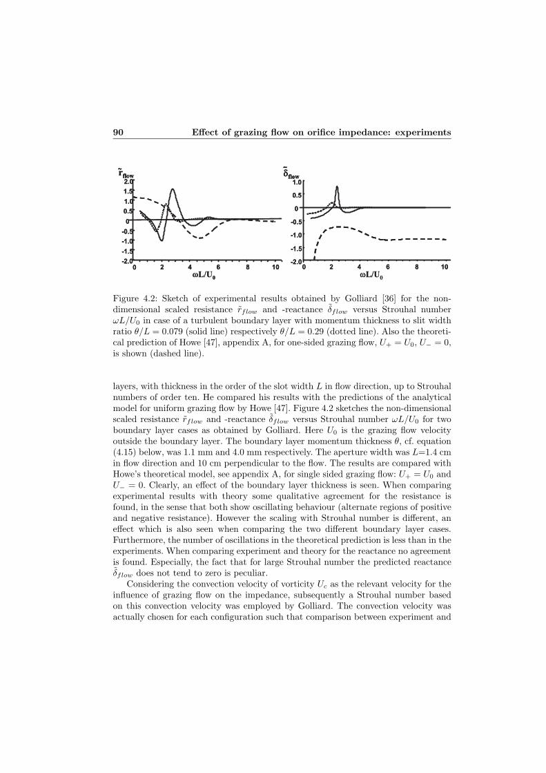
90 Effect of grazing flow on orifice impedance: experiments
�� � � �
�
� � � �
� � � � � �� � �
� �
� � �
� �
�
� �
�
� �
�
�
�� � � �
�
� � � �
� � � � � �� � �
� �
� � �
� �
�
� �
�
�
�� � � �
��� � � �
�
� � � �
� � � � � �� � �
� �
� � �
� �
�
� �
�
� �
�
�
�� � � �
��� � � �
�
� � � �
� � � � � �� � �
� �
� � �
� �
�
� �
�
�
Figure 4.2: Sketch of experimental results obtained by Golliard [36] for the non-dimensional scaled resistance rflow and -reactance δflow versus Strouhal numberωL/U0 in case of a turbulent boundary layer with momentum thickness to slit widthratio θ/L = 0.079 (solid line) respectively θ/L = 0.29 (dotted line). Also the theoreti-cal prediction of Howe [47], appendix A, for one-sided grazing flow, U+ = U0, U− = 0,is shown (dashed line).
layers, with thickness in the order of the slot width L in flow direction, up to Strouhalnumbers of order ten. He compared his results with the predictions of the analyticalmodel for uniform grazing flow by Howe [47]. Figure 4.2 sketches the non-dimensionalscaled resistance rflow and -reactance δflow versus Strouhal number ωL/U0 for twoboundary layer cases as obtained by Golliard. Here U0 is the grazing flow velocityoutside the boundary layer. The boundary layer momentum thickness θ, cf. equation(4.15) below, was 1.1 mm and 4.0 mm respectively. The aperture width was L=1.4 cmin flow direction and 10 cm perpendicular to the flow. The results are compared withHowe’s theoretical model, see appendix A, for single sided grazing flow: U+ = U0 andU− = 0. Clearly, an effect of the boundary layer thickness is seen. When comparingexperimental results with theory some qualitative agreement for the resistance isfound, in the sense that both show oscillating behaviour (alternate regions of positiveand negative resistance). However the scaling with Strouhal number is different, aneffect which is also seen when comparing the two different boundary layer cases.Furthermore, the number of oscillations in the theoretical prediction is less than in theexperiments. When comparing experiment and theory for the reactance no agreementis found. Especially, the fact that for large Strouhal number the predicted reactanceδflow does not tend to zero is peculiar.
Considering the convection velocity of vorticity Uc as the relevant velocity for theinfluence of grazing flow on the impedance, subsequently a Strouhal number basedon this convection velocity was employed by Golliard. The convection velocity wasactually chosen for each configuration such that comparison between experiment and

4.3 Previous experimental studies 91
�� � � �
�
� � � �
� � � � � �
� � �
� �
� � �
� �
�
� �
�
� �
�
� � � � �
�� � � �
�
� � � �
� � � � � �� � �
� �
� � �
� �
�
� �
�
� � � � �
�� � � �
��� � � �
�
� � � �
� � � � � �
� � �
� �
� � �
� �
�
� �
�
� �
�
� � � � �
�� � � �
��� � � �
�
� � � �
� � � � � �� � �
� �
� � �
� �
�
� �
�
� � � � �
Figure 4.3: Sketch of experimental results obtained by Golliard [36] for the non-dimensional scaled resistance rflow and -reactance δflow in case of a turbulent bound-ary layer with momentum thickness to slit width ratio θ/L = 0.079 (solid line) re-spectively θ/L = 0.29 (dotted line). Here the Strouhal number ωL/Uc is based onthe convection velocity of vorticity in the aperture. Also the theoretical prediction ofHowe [47], appendix A, for one-sided grazing flow (dashed line) as well as for a twosided grazing flow with U− = 0.2U+ (dot-dash line) is shown.
theory was best. From this it appeared that the relation: Uc/U0 = 0.4(δtu/L)−0.2
provided a reasonably good fit, where δtu is the turbulent boundary layer thickness,see section 4.6.1 below. The results for the same boundary layer cases as above, cf.figure 4.2, are shown in figure 4.3. The figure also shows the theoretical result for two-sided grazing flow, where U+ = U0 and U− = 0.2U0. Compared to one-sided grazingflow more oscillations are seen, giving a better (qualitative) agreement with experi-ments. Golliard therefore suggests that the velocity beneath the orifice, induced byentrainment, should be taken into account when analysing the behaviour of an orificewith one-sided imposed grazing flow. The experimental results of Golliard were firstconfirmed by the present author by measurements with a single microphone method[58]. Here, the change in orifice impedance due to grazing flow over a rectangular slotin a damped Helmholtz resonator was determined by measuring the transfer of soundfrom a loudspeaker outside the resonator to a microphone placed inside the resonator.These experiments will not be presented in this thesis.
Peat et al. [86] compared measurements on circular orifices both with Howe’stheory in its original form and with a modified form as proposed by Jing et al. [48].Regarding the original formulation of the theory basically the same conclusions weredrawn as in Golliard’s work [36]. The reactance predicted by the modified theorywas argued to yield better (qualitative) agreement with experimental results, whereasresistance prediction became worse. Especially negative resistance, found in some

92 Effect of grazing flow on orifice impedance: experiments
Strouhal ranges, was not predicted anymore. Furthermore, the vorticity convectionvelocity was not considered as the relevant velocity in comparing experiments with themodified theory, as opposed to comparison with the theory in the original formulation.
4.4 Impedance tube experiment
4.4.1 Setup
Acoustic measurements have been performed with an impedance tube in a semi-anechoic room. A multi-microphone layout is chosen in order to have better accu-racy in a relatively wide frequency range compared to a ’standard’ two microphoneimpedance tube set-up ([1, 10, 15, 20]). Figure 4.4 shows a picture of the setup, aschematic layout is given in figure 4.5. The set-up consists of a 70 cm long smoothsteel tube with an inner radius of R=3.5 cm and an outer radius of 5.5 cm. A total of 7microphones (PCB 116A) connected to charge amplifiers (Kistler 5011) are mountedin adapters in the wall of the tube. A signal generator (NI PXI-5411 arbitrary wave-form generator) sends a harmonic signal with angular frequency ω via an amplifier(Toellner TOE 7608) to the loudspeaker. The loudspeaker couples the sound into theimpedance tube at the back end through a piece of porous acoustical damping ma-
� � � ! � � � " � � # � � � � � $ � � % � & �
' � % � � � $ ( � � ! � % � � �
! � ! % � � � )
* � + � � � � + � � � � � % � �
, � � % � � � � �
� � � � + � � � � � � � � � � !
- � � � $ �
� � � ! � � � " � � # � � � � � $ � � % � & �
' � % � � � $ ( � � ! � % � � �
! � ! % � � � )
* � + � � � � + � � � � � % � �
, � � % � � � � �
� � � � + � � � � � � � � � � !
- � � � $ �
Figure 4.4: Picture of the impedance tube set-up

4.4 Impedance tube experiment 93
� � � ! � � � " � �
. � � � � � � �
* � + � � � + � � � � � % � � � )
' � % � � � $ ( � � ! � % � � �
� � $ � � � � � � �
- � � � � � � � � % � � � � �
# � � � � � $ � % � & �
, � � � � � � % � � � � � $ �
' � � � � � + � � � % � � � � �� � � ! � � � " � �
. � � � � � � �
* � + � � � + � � � � � % � � � )
' � % � � � $ ( � � ! � % � � �
� � $ � � � � � � �
- � � � � � � � � % � � � � �
# � � � � � $ � % � & �
, � � � � � � % � � � � � $ �
' � � � � � + � � � % � � � � �
Figure 4.5: Schematic layout of the impedance tube set-up
terial. The damping material serves to prevent unwanted high acoustic amplitudesdue to resonance. A plate with a rectangular slit is attached to the other end ofthe tube. The plate is positioned such that the orifice is centered above the tube.The geometries of the different slits used will be given further on. The plate is alsofixed to the nozzle of an open windtunnel, which generates the grazing flow over theslit. In order to prevent acoustical leaks, o-rings are placed between the microphoneadapters and the tube, as well as between the plate and the tube. The signals of themicrophone’s charge amplifiers as well as the function generator signal are digitallysampled by a dynamic signal acquisition (DSA) card (NI PXI-4472) at 10 kS/s. Boththe DSA card and the signal generator module are driven by an embedded controller(NI PXI-8176). The three units are housed in a NI PXI-1042 8-slot chassis. For asingle measurement microphone signals are recorded over a period of 100 s. Subse-quently, as post-processing lock-in amplification is performed on an integer number ofsignal periods to determine the complex amplitudes of the microphone signals. Fromthis the reflection coefficient at the end plate is calculated as described below.
4.4.2 Impedance measurement
Below the cut-on frequency of the first higher order acoustic mode in the tube (atf=2870 Hz), the acoustic pressure and velocity disturbance, p resp. u, in the tube arecomposed of a plane waves propagating to the right and a plane wave propagating tothe left. The complex amplitudes are given by:
p(x) = p+exp(−ik+x) + p−exp(ik−x), (4.8)
u(x) =1
ρ0c0(p+exp(−ik+x) − p−exp(ik−x)). (4.9)
94 Effect of grazing flow on orifice impedance: experiments
Here p± is the complex amplitude at x = 0 of the pressure wave travelling in positiverespectively negative x-direction, i.e. to the right and to the left in figure 4.5. In caseof no mean flow through the tube the wave number k± is equal in both directions.Accounting for visco-thermal damping of the acoustical waves at the walls of the tubeit is given by [53, 93, 110, 87]:
k± =ω
c0
(1 +
1 − i√2
1Sh
(1 +γ − 1√Pr
) − iSh2
(1 +γ − 1√Pr
− 12γγ − 1Pr
)), (4.10)
in the low frequency approximation, kR � 1, and for high shear numbers, Sh =R√ω/ν � 1. Here ν is the kinematic viscosity, γ the ratio of specific heats at constant
pressure respectively constant volume, and Pr is the Prandtl number. For air at roomtemperature: c0 = 344 ms−1, ν = 1.51 10−5 m2s−1, γ = 1.4, Pr = 0.71. In thecurrent experiments 0.03 < kR < 0.6, and the shear number ranges from Sh � 160for low frequency to Sh � 700 for high frequency. The first correction to ω/c0, whichis proportional to Sh−1, affects both phase velocity and damping of the acousticplane waves. Here, it is a value of about 2 10−3 for low frequency to 4 10−4 forhigh frequency. The second term, proportional to Sh−2, only affects the damping.In the present experiments it is in the order of 10−3 to 7 10−3 of the value of thefirst correction for high and low frequency respectively, and therefore negligible. Theeffect on the damping coefficient of the plane waves due to visco-thermal losses in thebulk, see for instance Pierce [89] and Peters [87], appears to be at least two orders ofmagnitude smaller than that due to the losses at the wall given above. Therefore, itis neglected here.
Equation (4.8) can be written for all positions x1..x7 of the 7 microphones, givingan overdetermined problem for p+ and p−:⎡
⎢⎣p(x1)
...p(x7)
⎤⎥⎦
︸ ︷︷ ︸pm
=
⎡⎢⎣
exp(−ik+x1) exp(ik−x1)...
...exp(−ik+x7) exp(ik−x7)
⎤⎥⎦
︸ ︷︷ ︸Mexp
[p+
p−
]. (4.11)
Here we take x = 0 at the position of the end plate wall at the inside of the tube. Themicrophone positions are: x1 = −20 mm, x2 = −70 mm, x3 = −170 mm, x4 = −310mm, x5 = −365 mm, x6 = −410 mm, x7 = −565 mm. The least squares solution of(4.11) is found by: [
p+
p−
]= (Mexp
T Mexp)−1MexpT · pm, (4.12)
where superscript T indicates the complex conjugate transpose. The impedance Zh−of the orifice, as defined in equation (4.7), is now given by:
Zh− =1
ρ0c0
p(0)uh
=S0
Stube
p+ + p−
p+ − p−, (4.13)

4.5 Orifice geometries 95
using equations (4.8) and (4.9). Here, from conservation of mass, the acoustic velocitythrough the orifice, uh, equals Stube/S0 times the acoustic velocity u(0) in the tube atx = 0. S0 and Stube are the (cross sectional) areas of the orifice and tube respectively.Note that in calculating the impedance by equation (4.13) the effect of visco-thermaldamping on the wavenumber is not included, since it is only a small correction in theorder of 10−3 at maximum. However, in calculating the complex pressure amplitudesp±, cf. equations (4.11,4.12), it is included, since it has a cumulative effect in the wavepropagation.
4.4.3 Accuracy
In order to increase accuracy the microphones are calibrated with respect to a refer-ence microphone. This is done by placing the reference microphone and the micro-phone to be calibrated in a closed end wall at the end of the impedance tube. In thisway the same sound pressure is imposed on the microphones. Any difference in themeasured complex amplitudes of the microphones results in a calibration factor. Thecalibration is done at several frequencies. In the subsequent acoustical measurementsthe reference microphone is placed at the position closest to the end wall. After cali-bration, the reflection coefficient R0 = p−
p+at a closed end wall is measured in order to
assess the accuracy of the set-up. Figure 4.6 shows the deviation of the absolute value|R0| from unity as well as the (deviation of the) phase φ of the reflection coefficientscaled to 2π radians. Both are O(10−3) (for frequencies up to 800 Hz). Note that thisis a systematic error. The reproducibility of the measurement (random error) is ob-served to be O(10−4). From these results the error in the measured non-dimensionalscaled resistance and reactance is estimated to be in the order of 10−2.
4.5 Orifice geometries
Measurements are done with different rectangular orifices. Schematic cross sectionsare given in figure 4.7. All slits are symmetrically positioned in a 1.5 cm thick 20cm × 20 cm aluminum plate. Four slits have width L=1 cm in flow direction andmeasure 5 cm perpendicular to the flow, cf. figure 4.7a through d. The first one has27◦ sharp edges both upstream and downstream. The second one, figure 4.7b, has asingle sharp 27◦ edge and a normal 90◦ edge. By rotating the plate half a turn thesharp or normal edge can be positioned upstream or downstream. The third orificegeometry, figure 4.7c, has a normal 90◦ edge on one side. At the other side a 0.1 mmthin phosphor bronze plate juts out 2 mm into the 12 mm wide slit in the plate,giving a sharp ”0◦” edge. Also here, both edges can be positioned either upstreamor downstream. The last 1 cm wide slit, figure 4.7d, has two normal 90◦ edges. Thedistance of the windtunnel outlet to the upstream edge is Lw =9.5 cm for these fourL = 1 cm orifices. By rotating the plate with the orifice given in figure 4.7d a quarter

96 Effect of grazing flow on orifice impedance: experiments
turn a slit with normal 90◦ edges upstream and downstream is obtained measuringL=5 cm in flow direction and measuring 1 cm perpendicular to the flow, cf. figure4.7e. Distance from windtunnel outlet to upstream edge is Lw=7.5 cm for this case.
4.6 Mean flow properties
4.6.1 Boundary layer characterization
In order to determine the grazing flow conditions at the upstream edge of the aper-ture boundary layer measurements have been performed. For this purpose a 5 µmhot-wire is used (Dantec 55P11 on a Dantec 55H20 support connected to Streamlinecta module 90C10). The hot-wire measurements are done at a sample rate of 4000 S/sfor 10 seconds. Different boundary layers have been realized by varying the main flowvelocity U0 outside the boundary layer and by tripping the flow at the windtunneloutlet. For this purpose a strip of sandpaper and a spoiler are used. Furthermore,measurements are done at distance Lw = 7.5 cm and Lw = 9.5 cm from the wind-tunnel outlet, corresponding to the different positions of the upstream edge of theaperture configurations used, cf. figure 4.7. The characteristics of the boundary layersbased on the hot-wire measurements are listed in table 4.1. Here ReLw
= U0Lw/ν isthe Reynolds number based on the windtunnel outlet to orifice distance Lw, δ99 is the
� / � 0 � � 1
� / � 0 � � 2
� / � 0 � � �
� / � 0 � � �
� � � � 1 � � 3 � � 4 � � � � � � � � � �
� � � � �
� / � 0 � � 5
� / � 0 � � 1
� / � 0 � � 2
� / � 0 � � �
� � � � 1 � � 3 � � 4 � � � � � � � � � �
� � � � �
6 6 7 � � 6 � � � 6� � � � � � �
Figure 4.6: Impedance tube measurements of the reflection coefficient R0 at a closedend wall. Absolute deviation of |R0| from unity and absolute value of the phase φ ofR0 scaled to 2π radians.

4.6 Mean flow properties 97
2 � � � �
� 5 � � �
� � � � � � �
� � � � �
�
� � � � �
� 5 � � �
� � � � � � �
� � � � �
�
� � � � �
� 5 � � �
� � � � � � �
� / � � � �
�
� 5 � � �
� � � � � � ��
� 5 � � �
� � 5 � � � ��
� � � � � � $ � 8 � � 9 � � & � % � � ! � � ! & � � � � � $ � 8 � � 9 � � � � ! % � � � � � � � � � � � ! % � � � �
$ � � � � � $ � 8 � � � � � � ! % � � � � � � � � � � � ! % � � � � � � � � � $ � 8 � : � � � & � % � � ! � � !
� � � � � 5 $ � 8 � : � � � & � % � � ! � � !
2 � � � �
� 5 � � �
� � � � � � �
� � � � �
�
2 � � � �
� 5 � � �
� � � � � � �
� � � � �
�
� � � � �
� 5 � � �
� � � � � � �
� � � � �
�
� � � � �
� 5 � � �
� � � � � � �
� / � � � �
�
� � � � �
� 5 � � �
� � � � � � �
� / � � � �
�
� 5 � � �
� � � � � � ��
� 5 � � �
� � � � � � ��
� 5 � � �
� � 5 � � � ��
� 5 � � �
� � 5 � � � ��
� � � � � � $ � 8 � � 9 � � & � % � � ! � � ! & � � � � � $ � 8 � � 9 � � � � ! % � � � � � � � � � � � ! % � � � �
$ � � � � � $ � 8 � � � � � � ! % � � � � � � � � � � � ! % � � � � � � � � � $ � 8 � : � � � & � % � � ! � � !
� � � � � 5 $ � 8 � : � � � & � % � � ! � � !
Figure 4.7: Schematical cross section of the different rectangular orifices used in ex-periments. Slits a through d measure L = 1 cm in grazing mean flow direction andhave width of 5 cm perpendicular to the flow. They differ in edge geometry. Asym-metrical slits (b and c), can be placed with their sharp edge either downstream (asdrawn) or upstream. Slit e has width L = 5 cm in flow direction and measures 1 cmperpendicular to the flow.

98 Effect of grazing flow on orifice impedance: experiments
boundary layer thickness where U(δ99)/U0=0.99, δ1 is the displacement thickness:
δ1 =∫ ∞
0
(1 − U(y)
U0
)dy, (4.14)
and θ is the momentum thickness of the boundary layer:
θ =∫ ∞
0
U(y)U0
(1 − U(y)
U0
)dy. (4.15)
The boundary layer profiles measured with the hot-wire are shown in figure 4.8. Itcan be seen that the profiles for Lw =7.5 cm are almost similar to the equivalentprofiles at Lw =9.5 cm. The largest difference here is seen for the spoiler-trippedboundary layer. Also the sandpaper tripped boundary layers with U0=16.8 m/s (V)and U0=34.1 m/s (VII) are almost similar.
The measured data for boundary layers I to IV and VIII are fitted with a laminarBlasius profile [102]. A very good fit is obtained for profile I at U0 = 4 m/s. Forincreasing velocities, boundary layers II to IV and VIII, the deviation from a Blasiusprofile becomes larger. The profiles V to VII and IX and X are fitted with a turbulentboundary layer velocity distribution given by the logarithmic law corrected with Coles’law of the wake [41]:
U(y)ufric
=1κ
ln(ufricy
ν) +B +
Πκ
(1 − cos(πy
δtu)), y ≤ δtu,
Π =κ
2U0
ufric− 1
2ln(
ufricδtuν
) − Bκ
2. (4.16)
Table 4.1: Characteristics of the different boundary layers measured.Boundary Lw U0 ReLw
tripping δ99 δ1 θ ufric/U0
layer (cm) (m/s) (mm) (mm) (mm)I 9.5 4.0 2.53 104 - 5.0 1.38 0.55II 9.5 6.0 3.80 104 - 3.8 1.10 0.46III 9.5 8.8 5.57 104 - 3.1 0.90 0.38IV 9.5 16.8 1.06 105 - 2.5 0.67 0.29V 9.5 16.8 1.06 105 sandpaper 7.2 1.16 0.83 0.048VI 9.5 16.8 1.06 105 spoiler 22.4 8.80 3.90 0.0175VII 9.5 34.1 2.16 105 sandpaper 7.3 1.16 0.81 0.044VIII 7.5 16.8 8.40 104 - 2.5 0.64 0.29IX 7.5 16.8 8.40 104 sandpaper 7.2 1.18 0.81 0.048X 7.5 16.8 8.40 104 spoiler 22.3 9.13 3.63 0.0135

4.6 Mean flow properties 99
0 2 4 6 8 100
0.2
0.4
0.6
0.8
1U(y)/U
0
y/θ
I
ReL
w
=2.53 104
0 2 4 6 8 100
0.2
0.4
0.6
0.8
1U(y)/U
0
y/θ
II
ReL
w
=3.80 104
0 2 4 6 8 100
0.2
0.4
0.6
0.8
1U(y)/U
0
y/θ
III
ReL
w
=5.57 104
0 2 4 6 8 100
0.2
0.4
0.6
0.8
1
IV (ReL
w
=1.06 105)
VIII (ReL
w
=8.40 104)
y/θ
U(y)/U0
0 2 4 6 8 100
0.2
0.4
0.6
0.8
1
VVIIIX
U(y)/U0
y/θ
Sandpaper tripped
0 1 2 3 4 5 6 70
0.2
0.4
0.6
0.8
1
VIX
U(y)/U0
y/θ
Spoiler tripped
Figure 4.8: Boundary layer profiles. Measured data are indicated with the markers,the solid lines give the corresponding fit. Profiles of boundary layers I, II, III, IV andVIII are fitted with a laminar Blasius profile [102]. Profiles of boundary layers V,VI, VII, IX and X are fitted with the logarithmic law for a turbulent boundary layercorrected with Coles’ law of the wake [41], eq. (4.16).

100 Effect of grazing flow on orifice impedance: experiments
Here ufric is the friction velocity. Table I gives the friction velocity obtained from thefit for the concerning boundary layers. B=5.1 is a boundary layer constant, κ=0.41 isthe von Karman constant, and δtu is the turbulent boundary layer thickness, whereU(δtu) = U0. Figure 4.8 shows reasonably good agreement between the measuredprofiles and the turbulent profile of equation (4.16).
In order to investigate the turbulence of the boundary layers more, the turbulentintensity Tu is considered. Following e.g. Schlichting [102], we define the turbulenceintensity here as the ratio of the root mean square of the turbulent velocity fluctuationsU ′ =
√U ′2
x + U ′2y perpendicular to the hot-wire and the velocity U0 outside the
boundary layer:
Tu =
√< U ′2 >U0
. (4.17)
Results are shown in figure 4.9. The turbulence intensity of the turbulent fitted bound-ary layers (i.e. numbers V, VI, VII, IX, and X), depicted in the lower two graphs offigure 4.9, is indeed larger than that of the laminar fitted boundary layers. However,especially for boundary layers IV and VIII the turbulence intensity is almost as largeas for the turbulent fitted ones. Although it is still reasonably well fitted with a lam-inar Blasius profile, these boundary layers can be regarded as on the transition fromlaminar to turbulent. For boundary layer flows I to V the mean flow velocity at thepoint where the highest turbulence intensity is measured is shown in figure 4.10 asfunction of time for the first second of the measurement. It is seen that for the laminarfitted boundary layers, no. I to IV, the velocity fluctuations occur more rapidly withincreasing main flow velocity. For the turbulent fitted boundary layer, no. V, veryrapid fluctuations are observed compared to all other boundary layer flows.
Overlooking the results above, the boundary layers I to III will be regarded aslaminar, whereas boundary layers IV and VIII are designated transitional. The sand-paper tripped boundary layers V, VII and IX are turbulent. Due to the pronouncedform of a wake behind an object, see figure 4.8, the spoiler tripped boundary layersVI and X will be designated as turbulent wake.
4.6.2 Shear layer profiles
In studying its acoustical response the flow properties of the shear layer developing inthe orifice are of interest. Therefore, hot-wire measurements of shear layer profiles aredone for the 1 cm orifices with double sharp 27◦ edges and with double 90◦ edges, aswell as for the 5 cm slit, cf. figure 4.7a, d and e respectively. Results for the 1 cm slotwith sharp edges are shown in figure 4.11 for boundary layer flows I to V. Shear layerprofiles at various distances from the upstream edge xs are depicted, viz. xs = 2 mm,xs = 4 mm, xs = 6 mm, and xs = 8 mm. Also, the boundary layer profiles are shown(xs = 0 mm). The y-coordinate on the horizontal axes is scaled to the momentumthickness θ0 of the boundary layer. Shear layer profiles for the 1 cm slot with double

4.6 Mean flow properties 101
0 2 4 6 8 100
0.01
0.02
0.03
0.04
0.05Tu
y/θ
I
ReL
w
=2.53 104
0 2 4 6 8 100
0.01
0.02
0.03
0.04
0.05
0.06
0.07Tu
y/θ
II
ReL
w
=3.80 104
0 2 4 6 8 100
0.02
0.04
0.06
0.08
0.1Tu
y/θ
III
ReL
w
=5.57 104
0 2 4 6 8 100
0.02
0.04
0.06
0.08
0.1
0.12
IV (ReL
w
=1.06 105)
VIII (ReL
w
=8.40 104)
y/θ
Tu
0 2 4 6 8 100
0.02
0.04
0.06
0.08
0.1
0.12
VVIIIX
Tu
y/θ
Sandpaper tripped
0 2 4 6 8 100
0.02
0.04
0.06
0.08
0.1
0.12
0.14
VIX
Tu
y/θ
Spoiler tripped
Figure 4.9: Turbulence intensity Tu of the different boundary layers.

102 Effect of grazing flow on orifice impedance: experiments
0 0.2 0.4 0.6 0.8 12.8
3
3.2U(t) (m/s)
0 0.2 0.4 0.6 0.8 12
4
6
0 0.2 0.4 0.6 0.8 10
5
10
0 0.2 0.4 0.6 0.8 10
10
20
0 0.2 0.4 0.6 0.8 10
10
20
t (s)
I
II
III
IV
V
Figure 4.10: Mean flow velocity as function of time at the point in the boundary layerwhere turbulence intensity is maximum, cf. figure 4.9, for boundary layer flows I toV.
90◦ edges are shown in figure 4.12 at the same distances xs for boundary layer flowsIV and V. For the 5 cm slot shear layer profiles for boundary layer flow VIII and IX(to be compared with boundary layer IV and V for the 1 cm slots) are shown in figure4.13 for various distances xs from the upstream edge.
The shear layer profiles of boundary layer IV and V for the 1 cm slot with sharpedges and the 1 cm slot with normal edges are nearly identical. However, for turbulentboundary layer flow V the measured velocity does not seem to tend to zero at the lowerside of the shear layer in case of the slot with normal edges. Here, the flow velocityremains more or less constant. Most probably this is caused by the fact that thereis a significant entrainment velocity. Comparing the geometries of the two orifices itcould be expected that the flow in the slot with normal edges will differ more from an’ideal’ parallel shear flow, especially near the upstream and downstream edge. In thecase of normal edges the entrainment velocity will have a strong component normalto the main flow. This is illustrated in figure 4.14, giving a sketch of the entrainedflow in the orifice for the two different geometries. The effect is also seen in shear layermeasurements closest to the upstream edge for the 5 cm slot especially with turbulentboundary layer IX.
Analogous to the boundary layer momentum thickness, the shear layer momentum

4.6 Mean flow properties 103
−5 0 5 100
0.2
0.4
0.6
0.8
1
y/θ0
U(y)/U0 I
−5 0 5 100
0.2
0.4
0.6
0.8
1
y/θ0
U(y)/U0 II
−5 0 5 100
0.1
0.2
0.3
0.4
0.5
0.6
0.7
0.8
0.9
1
y/θ0
U(y)/U0 III
−5 0 5 100
0.2
0.4
0.6
0.8
1
y/θ0
U(y)/U0 IV
−5 0 5 100
0.2
0.4
0.6
0.8
1
y/θ0
U(y)/U0 V
Figure 4.11: Shear layer profile measurements at various distances xs from the up-stream edge for the 1 cm slot with double 27◦ edges, cf. figure 4.7a, and boundarylayer flow I to V. ◦ markers: xs = 0 mm (boundary layer profile), + markers: xs = 2mm, ∇ markers: xs = 4 mm, ∗ markers: xs = 6 mm, × markers: xs = 8 mm. They-coordinate is scaled to the boundary layer momentum thickness θ0.

104 Effect of grazing flow on orifice impedance: experiments
−5 0 5 100
0.2
0.4
0.6
0.8
1
y/θ0
U(y)/U0 IV
−5 0 5 100
0.2
0.4
0.6
0.8
1
y/θ0
U(y)/U0 V
Figure 4.12: Shear layer profile measurements at various distances xs from the up-stream edge for the 1 cm slot with double 90◦ edges, cf. figure 4.7d, and boundarylayer flow IV and V. ◦ markers: xs = 0 mm (boundary layer profile), + markers:xs = 2 mm, ∇ markers: xs = 4 mm, ∗ markers: xs = 6 mm, × markers: xs = 8 mm.The y-coordinate is scaled to the boundary layer momentum thickness θ0.
−50 −40 −30 −20 −10 0 10 200
0.2
0.4
0.6
0.8
1
y/θ0
U(y)/U0 VIII
−15 −10 −5 0 5 100
0.2
0.4
0.6
0.8
1
y/θ0
U(y)/U0 IX
Figure 4.13: Shear layer profile measurements at various distances xs from the up-stream edge for the 5 cm slot with double 90◦ edges, cf. figure 4.7e, and boundarylayer flow VIII and IX. ◦ markers: xs = 0 mm (boundary layer profile), + markers:xs = 5 mm, ∇ markers: xs = 10 mm, ∗ markers: xs = 20 mm, × markers: xs = 30mm, � markers: xs = 40 mm for BL VIII or xs = 35 mm for BL IX. The y-coordinateis scaled to the boundary layer momentum thickness θ0.

4.6 Mean flow properties 105
� � � � & �� � � � & �
Figure 4.14: Sketch of the entrained flow in the orifice with normal 90◦ edges (a) andwith 27◦ edges (b). In the former geometry the vertical velocity component near theupstream and downstream edge will be relatively large.
thickness is given by (see also equation B.9):
θ =∫ ∞
−∞
U(y)U0
(1 − U(y)
U0
)dy. (4.18)
The momentum thickness as function of the distance from the upstream edge calcu-lated for the experimental data above is shown in figure 4.15 for the 1 cm slot withsharp edges for boundary layer flows I to V. For all boundary layer flows the data canbe fitted well with a straight line, giving a linear increase of momentum thickness withdistance. For the 5 cm slot momentum thickness as function of distance to upstreamedge is depicted in figure 4.16. For the turbulent boundary layer IX a linear fit ap-plies. As shown in the graph this fit agrees well with that applied to the data for thecorresponding turbulent boundary layer V in case of the 1 cm slot with sharp edges(figure 4.15). For the transitional boundary layer VIII a linear increase in momentumthickness with distance is seen up to xs = 10 mm. The linear fit applied to the data ofthe corresponding transitional boundary layer IV in case of the 1 cm slot with sharpedges, cf. figure 4.15, also applies reasonably well to these points. However, for largerdistances from the upstream edge a stronger increase in momentum thickness is seen.Note that, in calculating the momentum thickness, for those cases in which a nonzerovelocity is measured at the lower side of the shear layer due to the entrained normalvelocity, an estimate of the (parallel) profile there is made. The error in the calculatedvalues for θ/θ0 is estimated at ±5%. Furthermore, due to experimental constraintsthe shear layer profiles for the spoiler tripped turbulent wakes VI and X have notbeen measured.

106 Effect of grazing flow on orifice impedance: experiments
0 2 4 6 8 100.9
1
1.1
1.2
1.3
1.4
1.5
1.6
xs (mm)
I II
III
IV
V
θ/θ0
Figure 4.15: Shear layer momentum thickness θ scaled by the corresponding boundarylayer momentum thickness θ0 against distance xs from the upstream edge for the 1cm slot with double 27◦ edges. + markers: BL I, ∗ markers: BL II, ∇ markers: BLIII, ◦ markers: BL IV, � markers: BL V. A linear fit is applied to each data series.
0 10 20 30 40 50
1
2
3
4
5
6
7
8θ/θ
0
xs (mm)
Figure 4.16: Shear layer momentum thickness θ scaled by the corresponding boundarylayer momentum thickness θ0 versus distance xs from the upstream edge for the 5 cmslot. ◦ markers: BL VIII, ∗ markers: BL IX. Solid line: linear fit of data for BL IX.Dashed and dotted line: linear fit of data for BL IV respectively BL V in case of 1cm slot with sharp edges, cf. figure 4.15.

4.7 Results 107
4.7 Results
4.7.1 Impedance without mean flow
The measured impedance in case mean flow is absent is shown in figure 4.17 forthe various slots with different edge geometry, cf. figure 4.7. The real part of theimpedance, i.e. the resistance r, increases with frequency. Results for the differentorifice geometries are in general quite close. Between 500 Hz and 700 Hz some de-viation is seen for the double 27◦ edge geometry compared to the others. At highfrequency the resistance for the single sharp 0◦ edge geometry is higher than for theother geometries.
For monopole radiation the resistance is proportional to the square of the Helmholtznumber based on the characteristic orifice dimension. As expected, the imaginary partof the impedance increases linearly with frequency, with different slope for the differ-ent edge geometries. The imaginary part of the impedance is namely proportional tothe Helmholtz number with a constant related to the inertia of the fluid motion inthe orifice, see also equation (4.4). Figure 4.18 shows the real part of the impedancescaled to the square of the Helmholtz number k0Re based on the hydraulic radiusRe of the aperture as well as the imaginary part of the impedance divided by theHelmholtz number k0Re. Here, the hydraulic radius of the orifice is the equivalent ra-
dius of a circular orifice with the same area: Re =√
S0π . For the scaled resistance very
large values are seen below k0Re = 0.05 (which corresponds to a frequency of about
0 200 400 600 800 10000
0.02
0.04
0.06
0.08
0.1
0.12
0.14
0.16
0.18
f (Hz)
ℜ(Zh−
)
0 200 400 600 800 10000
0.1
0.2
0.3
0.4
0.5
0.6
0.7
f (Hz)
ℑ(Zh−
)
Figure 4.17: Real part and imaginary part of the aperture impedance Zh− of the slotswith different edge geometries, cf. figure 4.7. × markers: double sharp 27◦ edges, ∗markers: single sharp 27◦ edge, ◦ markers: normal 90◦ edges, ∇ markers: single sharp0◦ edge.

108 Effect of grazing flow on orifice impedance: experiments
0 0.05 0.1 0.15 0.2 0.250
0.5
1
1.5
2
2.5
3
3.5
4ℜ(Z
h−)/(k
0R
e)2
k0R
e0 0.05 0.1 0.15 0.2 0.25
1.2
1.4
1.6
1.8
2
2.2
2.4
2.6ℑ(Z
h−)/(k
0R
e)
k0R
e
Figure 4.18: Real and imaginary part of the aperture impedance Zh−, scaled to theHelmholtz number squared resp. the Helmholtz number, for the slots with differentedge geometries, cf. figure 4.7. × markers: double sharp 27◦ edges, ∗ markers: singlesharp 27◦ edge, ◦ markers: normal 90◦ edges, ∇ markers: single sharp 0◦ edge.
f = 200 Hz). This is most probably due to the limited accuracy of the measurement,as for low frequency the resistance is very small. Between a frequency of f = 200Hz and f = 800 Hz, corresponding to k0Re between 0.05 and 0.2, the value for thescaled resistance is reasonably constant between 0.5 and 1. For higher frequency againlarge values are seen. Possible explanations for this are the decreased measurementaccuracy for especially the absolute value of the reflection coefficient above f = 800Hz, see also figure 4.6, and the effect of higher order radiation.
According to equation (4.4), the imaginary part of the impedance divided byHelmholtz number k0Re equals the ratio of reactance δ to hydraulic radius Re. For allorifice geometries the observed values in figure 4.18 are fairly constant with frequency.Only at higher frequencies some deviation is found. As expected the value of thereactance for the different orifice geometries increases in the following order: doublesharp 27◦ edges, single sharp 27◦ edge, single sharp 0◦ edge, and normal 90◦ edges.For the orifice with normal 90◦ edges the plate thickness (equal to 1.5 cm, or 1.19Re)can simply be subtracted from the reactance δ to obtain an end correction. This endcorrection is then about equal to the hydraulic radius Re.
The accuracy of reflection coefficient measurements, addressed in section 4.4.3above, in relation to the orifice impedance without flow is studied more in figure 4.19.Here, the expected reflection coefficient R in case the orifice impedance is Zh− =0.5(k0R2)2 +i1.8k0Re, representative for the experimental results above, is comparedto the error in the reflection coefficient at a closed wall. The figure shows the value of|1− |R|| and |φ/2π|, with φ the phase of the reflection coefficient, for both the orifice
4.7 Results 109
0 0.05 0.1 0.15 0.2 0.2510
−4
10−3
10−2
10−1
k0R
e
|1−|R||
0 0.05 0.1 0.15 0.2 0.2510
−5
10−4
10−3
10−2
10−1
100
k0R
e
|φ/2π|
Figure 4.19: Magnitude and phase of the reflection coefficient R for an impedanceZh− = 0.5(k0Re)2 + i1.8k0Re (solid lines) compared to the error in R in case of aclosed end wall (solid lines with × markers), cf. figure 4.6.
impedance mentioned above and for the measurements at a closed wall, cf. figure 4.6,as function of Helmholtz number k0Re. It is observed that for low and high frequencythe deviation of the absolute value of the reflection coefficient from unity, expectedfor the mentioned impedance, is of the same order as the error. In between, the erroris about an order in magnitude smaller than the ’measured’ value. The error in thephase of the reflection coefficient is at least an order of magnitude smaller than the’measured’ value. Thus indeed for low and high frequencies a relatively large error inthe measured impedance, especially observed above for the real part, is expected.
4.7.2 Impedance with grazing mean flow
Figure 4.20 shows the measured impedance Zh−, cf. equation (4.7), for the L=1 cmorifice with double sharp 27◦ edges as function of frequency f in case no mean flowis present, and in case of grazing mean flow with turbulent boundary layer V. Thedifference in impedance due to the flow is depicted in figure 4.21. With grazing flow thevalue of the impedance (both real and imaginary part) oscillates around the no flowvalue. At low frequency the flow increases the resistance, here absorption of soundoccurs. For increasing frequency this effect diminishes, and at around f=320 Hz aregion starts where the resistance is decreased by the grazing flow. In this region theresistance with flow becomes negative, this means sound production takes place. Atabout f=590 Hz there is a minimum in the resistance, after which a sharp transitionto a second region of sound absorption is seen. The increase in resistance due to the
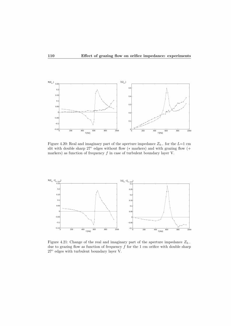
110 Effect of grazing flow on orifice impedance: experiments
0 200 400 600 800 1000−0.15
−0.1
−0.05
0
0.05
0.1
0.15
0.2
0.25ℜ(Z
h−)
f (Hz)0 200 400 600 800 1000
0
0.1
0.2
0.3
0.4
0.5
f (Hz)
ℑ(Zh−
)
Figure 4.20: Real and imaginary part of the aperture impedance Zh− for the L=1 cmslit with double sharp 27◦ edges without flow (∗ markers) and with grazing flow (+markers) as function of frequency f in case of turbulent boundary layer V.
0 200 400 600 800 1000−0.15
−0.1
−0.05
0
0.05
0.1
0.15
0.2
0.25
f (Hz)
ℜ(Zh−
−Zh−,U=0
)
0 200 400 600 800 1000−0.1
−0.05
0
0.05
0.1
0.15
0.2
0.25
0.3
f (Hz)
ℑ(Zh−
−Zh−,U=0
)
Figure 4.21: Change of the real and imaginary part of the aperture impedance Zh−due to grazing flow as function of frequency f for the 1 cm orifice with double sharp27◦ edges with turbulent boundary layer V.

4.7 Results 111
flow in this region is much larger than at low frequencies. The sharp transition in theresistance coincides with a peak in the imaginary part of the impedance. In a regionof about f = 500 Hz to f = 700 Hz around this peak the effect of the flow is toincrease the imaginary part of the impedance, and therefore the reactance, whereasoutside this region the reactance is decreased by the flow. Globally, for this particularboundary layer case the effect of the grazing flow on the impedance is quite largecompared to the value of the impedance without flow.
4.7.3 Linearity
The linearity of the orifice impedance with grazing flow is investigated by measuringat different sound pressure levels. Results for the L=1 cm slot with double sharp27◦ edges with turbulent boundary layer V at several frequencies are plotted in figure4.22. The graphs show the relative change of the real and imaginary part of the orificeimpedance Zh− with respect to a reference value Zh−,ref as function of the amplitudeof the acoustic velocity through the orifice |uh| over the mean flow velocity U0. Thevalue of the impedance at the lowest acoustic velocity amplitude is taken as referenceZh−,ref . Note that the scale |uh|/U0 = 10−4 to |uh|/U0 = 1 in figure 4.22 correspondsto sound pressure levels from about 70 dB up to 150 dB just beneath the orifice.
10−4
10−3
10−2
10−1
100
−2.5
−2
−1.5
−1
−0.5
0
0.5
1
1.5
|uh|/U
0
(ℜ(Zh−
) − ℜ(Zh−,ref
)) / ℜ(Zh−,ref
)
10−4
10−3
10−2
10−1
100
−0.6
−0.5
−0.4
−0.3
−0.2
−0.1
0
0.1
0.2
0.3
|uh|/U
0
(ℑ(Zh−
) − ℑ(Zh−,ref
)) / ℑ(Zh−,ref
)
Figure 4.22: Relative change of the orifice impedance Zh− with respect to a referencevalue Zh−,ref for the 1 cm orifice with double sharp 27◦ edges in case of turbulentboundary layer V as function of the amplitude of the acoustic velocity through theorifice |uh| over the mean flow velocity U0. For Zh−,ref the value at the lowest acousticvelocity amplitude is taken. � markers: f = 48 Hz, × markers: f = 302 Hz, + markers:f = 588 Hz, ∗ markers: f = 609 Hz, ◦ markers: f = 660 Hz, ∇ markers: f = 898 Hz.

112 Effect of grazing flow on orifice impedance: experiments
For the lowest frequency, f=48 Hz, linear behaviour is observed up to a relativeamplitude |uh|/U0 = 0.2 for the real part and up to |uh|/U0 = 5 · 10−2 for the imagi-nary part of the impedance. At f=302 Hz, just before the resistance becomes negative,see figure 4.20, impedance is linear up to a relative amplitude |uh|/U0 of 10−2. Strongnonlinear behaviour is only seen for |uh|/U0 larger than 0.1. For the frequencies f=588Hz and f=660 Hz, at which the resistance has a minimum respectively maximum, cf.figure 4.20, the onset of nonlinear behaviour is at approximately |uh|/U0 = 2 · 10−3.For f=609 Hz, corresponding to the sharp transition from negative to positive resis-tance and the peak in the imaginary part of the impedance, cf. figure 4.20, the onsetof nonlinearity seems to be at even lower amplitude: at about |uh|/U0 = 3 · 10−4.At a frequency of f=898Hz, beyond the strong oscillations in impedance, linearity isobserved up to |uh|/U0 several times 10−3.
Considering the deviations in the impedance from the (linear) reference value ata given amplitude, the effect of nonlinearity increases from f=48 Hz to subsequentlyf=302, f=898 Hz, f=660 Hz, f=588 Hz and f=609 Hz. Nonlinearity thus seems tobe strongest in the region where the oscillations in impedance are observed, here theonset of nonlinear behaviour is at lower amplitudes and the deviation from the linearimpedance is largest.
In following measurements on the linear behaviour of the orifice impedance undergrazing flow the acoustic amplitudes are mostly close to the onset of nonlinearity, inorder to have maximum signal amplitude.
4.7.4 Non-dimensional scaled resistance and reactance
Figures 4.23 and 4.24 show the non-dimensional scaled resistance and reactance, asdefined in equation (4.7), for the L=1 cm orifice with double 27◦ edges for the dif-ferent boundary layer flows. Non-dimensional scaled resistance and reactance for theL=5 cm aperture are depicted in figure 4.25. The results are plotted versus theStrouhal number ωL/U0 based on the orifice width in stream wise direction and themain flow velocity outside the boundary layer. For the L=1 cm orifice similar featuresare seen for all boundary layers. For increasing Strouhal number about 4 regions areobserved. For low Strouhal number resistance is positive, implying sound absorption.For higher Strouhal number a region is found where resistance is negative, imply-ing sound production due to the grazing flow. Subsequently, two more regions ofalternately positive and negative resistance follow. A similar oscillating behaviour isseen for the reactance. For both resistance and reactance the oscillations damp outfor high Strouhal number. The Strouhal numbers of the oscillations in the reactancemore or less coincide with those of the oscillations in the resistance. These specificfeatures in resistance and reactance generally shift to a higher Strouhal number fordecreasing boundary layer thickness. Furthermore, the amplitudes of the oscillationsincrease with decreasing laminar/transitional boundary layer thickness (BL I to IV).For the turbulent boundary layer V larger oscillations in the resistance and reactance

4.7 Results 113
0 1 2 3 4 5−0.4
−0.3
−0.2
−0.1
0
0.1
0.2
0.3
ω L/U0
~rflow
I θ
0/L=0.055
0 1 2 3 4 5−0.5
−0.4
−0.3
−0.2
−0.1
0
0.1
ω L/U0
~δflow
I θ
0/L=0.055
0 1 2 3 4 5−0.6
−0.4
−0.2
0
0.2
0.4
0.6
ω L/U0
~rflow
II θ
0/L=0.046
0 1 2 3 4 5−0.7
−0.6
−0.5
−0.4
−0.3
−0.2
−0.1
0
0.1
0.2
0.3
ω L/U0
~δflow
II θ
0/L=0.046
0 1 2 3 4 5−0.8
−0.6
−0.4
−0.2
0
0.2
0.4
0.6
0.8
1.0
1.2
ω L/U0
~rflow
III θ
0/L=0.038
0 1 2 3 4 5−0.8
−0.6
−0.4
−0.2
0
0.2
0.4
0.6
ω L/U0
~δflow
III θ
0/L=0.038
Figure 4.23: Non-dimensional scaled resistance and reactance due to grazing meanflow for the L=1 cm orifice with double 27◦ edges for boundary layers I, II and III.The boundary layer momentum thickness θ0 scaled to the slit width L is indicatedfor each case.

114 Effect of grazing flow on orifice impedance: experiments
0 1 2 3 4 5−10
−5
0
5
10
15
ω L/U0
~rflow
IV θ
0/L=0.029
0 1 2 3 4 5−2
−1
0
1
2
3
4
5
ω L/U0
~δflow
IV θ
0/L=0.029
0 1 2 3 4 5−10
−8
−6
−4
−2
0
2
4
ω L/U0
~rflow
x: V θ
0/L=0.083, +: VII θ
0/L=0.081
0 1 2 3 4 5−1.5
−1
−0.5
0
0.5
1
1.5
2
2.5
3
ω L/U0
~δflow
x: V θ
0/L=0.083, +: VII θ
0/L=0.081
0 1 2 3 4 5−0.4
−0.3
−0.2
−0.1
0
0.1
0.2
0.3
ω L/U0
~rflow
VI θ
0/L=0.39
0 1 2 3 4 5−0.6
−0.5
−0.4
−0.3
−0.2
−0.1
0
0.1
0.2
0.3
ω L/U0
~δflow
VI θ
0/L=0.39
Figure 4.24: Non-dimensional scaled resistance and reactance due to grazing meanflow for the L=1 cm orifice with double 27◦ edges for boundary layers IV, V, VIand VII. The boundary layer momentum thickness θ0 scaled to the slit width L isindicated for each case.

4.7 Results 115
0 2 4 6 8 10 12 14 16−2.5
−2
−1.5
−1
−0.5
0
0.5
1
1.5
2
ω L/U0
~rflow
VIII θ
0/L=0.0058
0 2 4 6 8 10 12 14 16−0.4
−0.3
−0.2
−0.1
0
0.1
0.2
0.3
0.4
0.5
ω L/U0
~δflow
VIII θ
0/L=0.0058
0 2 4 6 8 10 12 14 16−0.4
−0.2
0
0.2
0.4
0.6
0.8
1
ω L/U0
~rflow
IX θ
0/L=0.0162
0 2 4 6 8 10 12 14 16−0.4
−0.3
−0.2
−0.1
0
0.1
0.2
0.3
ω L/U0
~δflow
IX θ
0/L=0.0162
0 2 4 6 8 10 12 14 16−0.03
−0.02
−0.01
0
0.01
0.02
0.03
0.04
ω L/U0
~rflow
X θ
0/L=0.0726
0 2 4 6 8 10 12 14 16−0.02
−0.01
0
0.01
0.02
0.03
ω L/U0
~δflow
X θ
0/L=0.0726
Figure 4.25: Non-dimensional scaled resistance and reactance due to grazing meanflow for the L=5 cm orifice for boundary layers VIII, IX and X. The boundary layermomentum thickness θ0 scaled to the slit width L is indicated for each case.

116 Effect of grazing flow on orifice impedance: experiments
are observed than for the laminar boundary layers I to III, although the boundarylayer thickness of V is generally larger than those of I to III. For the spoiler trippedturbulent wake VI qualitatively the same features for the resistance and reactance asdiscussed are observed up to a Strouhal number of 1.7. However, for larger Strouhalnumber especially the resistance is not found to damp out to 0 (at least up to thelargest Strouhal number measured). The results for turbulent boundary layer flows Vand VII, which have nearly the same characteristics but different Mach number, arevery close, although the first peak of negative resistance at ωL/U0 � 2 is stronger forBL VII.
For the L=5 cm orifice more oscillations in resistance and reactance are found.Furthermore, for the turbulent wake boundary layer X less clearly defined behaviouris found. In this case the error in the measurements is of the same order as themeasured effect itself. For the transitional boundary layer VIII, the thinnest one,most oscillations are seen. Also the oscillations are at a higher Strouhal number andhave a larger amplitude compared to the turbulent boundary layer IX case. Thisis the same as seen in mutually comparing the correspondent boundary layers IVrespectively V for the L=1 cm orifice. Furthermore, in the results for transitionaland turbulent boundary layers VIII respectively IX the first resonance in resistanceand reactance has a smaller amplitude and seems to be at a slightly higher Strouhalnumber, compared to their corresponding cases for the L=1 cm slot.
4.7.5 Effective Strouhal number
As pointed out by others, e.g. Golliard [36], the impedance of the orifice is closelyconnected to the hydrodynamic instability of the shear layer developing in the orifice.A better way to compare orifice impedance results for different boundary layers wouldtherefore be to consider them as a function of the Strouhal number based on thephase velocity Uc of the hydrodynamic instability wave, i.e. the convection velocity ofvorticity in the aperture, rather than as function of the Strouhal number based on themain flow velocity U0. Golliard [36] used the convection velocity as a fit parameter toget a better agreement with the theoretical prediction of Howe [47], see section 4.3above. Goldman and Panton [34] for instance also discussed the use of an effectiveconvection velocity, although they gave it a more general interpretation.
Here we attempt to use calculations of the convective velocity of hydrodynamicinstability in a shear layer with generalized hyperbolic-tangent form as presentedby Michalke [67, 68], see appendix B.2. As shown there, for given profile, set bythe profile parameter m, the phase velocity Uc of the hydrodynamic instability non-dimensionalized by the mean flow velocity U0 is a function of the Strouhal numberbased on the momentum thickness θ of the shear layer and U0, cf. figure B.3:
Uc
U0= f(
ωθ
U0,m) (4.19)

4.7 Results 117
Since the form of the shear layer changes and the momentum thickness increases withdistance from the upstream edge, no unambiguous convection velocity can be found.An indication of the margin encountered in the scaling can be given by consideringthe boundary layer profile at the upstream edge, and the shear layer profile at thedownstream edge. The values of the momentum thickness for these profiles can beextracted from section 4.6 for the different experimental configurations. Concerningthe form of the shear layers, it is found that generally a reasonably good fit can beobtained between experiments, cf. figures 4.11, 4.12 and 4.13, and the generalizedhyperbolic-tangent profile, equation B.8. This is illustrated in figure 4.26, where themeasured shear layer profiles for the 1 cm orifice with double 27◦ edges and transitionalboundary layer flow IV are fitted with equation B.8. The values of the shear layermomentum thickness used in the fits is close to those calculated from the measuredprofiles, cf. figure 4.15. As shown, the profile parameter m varies between ∞ for theboundary layer to m = 1.5 for the shear layer 8 mm from the upstream edge. Thehyperbolic-tangent profiles are shifted in the y-direction as to give the best fit withexperimental data. For the boundary layer this actually gives a slight offset in thewall position. Note that shifting the fit profiles does not affect the calculated phasevelocity. For the turbulent boundary layer flows, no. V for the 1 cm slots and no. IXfor the 5 cm slot, and for the 5 cm slot with transitional boundary layer flow VIII
−5 0 5 100
0.2
0.4
0.6
0.8
1
y/θ0
U(y)/U0 IV
Figure 4.26: Measured shear layer profiles (markers) for the 1 cm wide orifice withdouble 27◦ edges with transitional boundary layer flow IV, cf. figure 4.11, fitted withthe hyperbolic-tangent profile (corresponding solid lines), equation (B.8), for differentdistances from upstream edge xs. ◦ markers: xs = 0 mm (boundary layer profile),θ = θ0 = 0.29 mm, profile parameter m = ∞. + markers: xs = 2 mm, θ = 0.32 mm,m = 5. ∇ markers: xs = 4 mm, θ = 0.35 mm, m = 3. ∗ markers: xs = 6 mm, θ = 0.39mm, m = 2. × markers: xs = 8 mm, θ = 0.44 mm, m = 1.5.

118 Effect of grazing flow on orifice impedance: experiments
shear layer profiles could be fitted less well with the generalized hyperbolic-tangentprofile than shown in the figure above.
The measured resistance and reactance for the 1 cm orifice with double 27◦ edgesand transitional boundary layer flow IV, cf. figure 4.24, can now be plotted versus theStrouhal number based on the convection velocity, calculated for either the boundarylayer profile or the shear layer profile at the downstream edge. For the boundary layerprofile θ = θ0 = 0.29 mm and m = ∞. The shear layer profile at the downstream edgeis not measured, however the momentum thickness can be estimated at θ = 1.6θ0 =0.46 mm using figure 4.15. The profile parameter is chosen m = 1 on basis of figure4.26. Results are shown in figure 4.27. A significant range in the Strouhal number isobserved. The oscillation in the resistance and corresponding peak in reactance is atωL/Uc ≈ 4 or at ωL/Uc ≈ 6 respectively, when Uc is calculated for the boundarylayer profile at the upstream edge or for the shear layer profile at the downstreamedge.
A scaling of the Strouhal number is done for the experiments with the 1 cmslit with double 27◦ edges for boundary layer flows I to V, depicted in figures 4.23and 4.24. The convective velocity is calculated from Michalke’s results for a shearlayer profile halfway the slot, at xs = 5 mm. The profile parameter is taken m = 2,providing a reasonably good fit with measured shear layer profiles. The momentumthickness at xs = 5 mm is determined from figure 4.15. Results are shown in figure4.28 and 4.29. In the graphs also a vertical dotted line is drawn. This line indicates
0 2 4 6 8 10−10
−5
0
5
10
15~rflow
ω L/Uc
0 2 4 6 8 10−2
−1
0
1
2
3
4
5
ω L/Uc
~δflow
Figure 4.27: Non-dimensional scaled resistance and reactance for the 1 cm orifice withdouble 27◦ edges and transitional boundary layer flow IV versus Strouhal numberbased on the convection velocity Uc of the hydrodynamic instability. × markers: Uc
calculated for the boundary layer: θ = θ0 = 0.29 mm,m = ∞. ∗ markers: Uc calculatedfor the shear layer at downstream edge: θ = 1.6θ0 = 0.46 mm, m = 1.
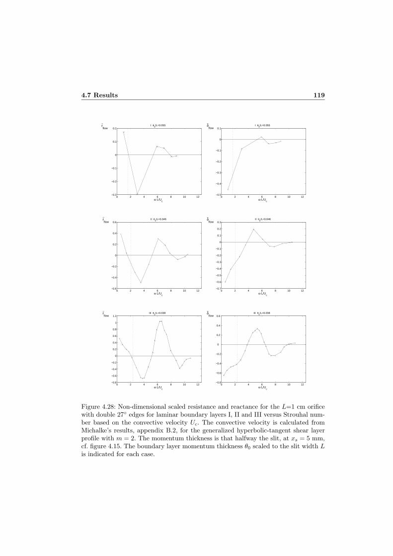
4.7 Results 119
0 2 4 6 8 10 12−0.3
−0.2
−0.1
0
0.1
0.2
ω L/Uc
~rflow
I θ
0/L=0.055
0 2 4 6 8 10 12−0.5
−0.4
−0.3
−0.2
−0.1
0
0.1
ω L/Uc
~δflow
I θ
0/L=0.055
0 2 4 6 8 10 12−0.6
−0.4
−0.2
0
0.2
0.4
0.6
ω L/Uc
~rflow
II θ
0/L=0.046
0 2 4 6 8 10 12−0.7
−0.6
−0.5
−0.4
−0.3
−0.2
−0.1
0
0.1
0.2
0.3
ω L/Uc
~δflow
II θ
0/L=0.046
0 2 4 6 8 10 12−0.8
−0.6
−0.4
−0.2
0
0.2
0.4
0.6
0.8
1
1.2
ω L/Uc
~rflow
III θ
0/L=0.038
0 2 4 6 8 10 12−0.8
−0.6
−0.4
−0.2
0
0.2
0.4
0.6
ω L/Uc
~δflow
III θ
0/L=0.038
Figure 4.28: Non-dimensional scaled resistance and reactance for the L=1 cm orificewith double 27◦ edges for laminar boundary layers I, II and III versus Strouhal num-ber based on the convective velocity Uc. The convective velocity is calculated fromMichalke’s results, appendix B.2, for the generalized hyperbolic-tangent shear layerprofile with m = 2. The momentum thickness is that halfway the slit, at xs = 5 mm,cf. figure 4.15. The boundary layer momentum thickness θ0 scaled to the slit width Lis indicated for each case.

120 Effect of grazing flow on orifice impedance: experiments
0 2 4 6 8 10 12−10
−5
0
5
10
15
ω L/Uc
~rflow
IV θ
0/L=0.029
0 2 4 6 8 10 12−2
−1
0
1
2
3
4
5
ω L/Uc
~δflow
IV θ
0/L=0.029
0 2 4 6 8 10 12−3
−2
−1
0
1
2
3
4
ω L/Uc
~rflow
V θ
0/L=0.083
0 2 4 6 8 10 12−1.5
−1
−0.5
0
0.5
1
1.5
2
2.5
3
ω L/Uc
~δflow
V θ
0/L=0.083
Figure 4.29: Non-dimensional scaled resistance and reactance for the L=1 cm orificewith double 27◦ edges for transitional boundary layer IV and turbulent boundarylayer V against Strouhal number based on the convective velocity Uc. The convec-tive velocity is calculated from Michalke’s results, appendix B.2, for the generalizedhyperbolic-tangent shear layer profile with m = 2. The momentum thickness is thathalfway the slit, at xs = 5 mm, cf. figure 4.15. The boundary layer momentum thick-ness θ0 scaled to the slit width L is indicated for each case.

4.7 Results 121
the Strouhal number ωL/Uc at which ωθ/U0 = 0.07. For values ωθ/U0 ≤ 0.07, andthus Strouhal numbers ωL/Uc less than the value indicated by the line, the convectionvelocity is independent of profile parameter m, cf. figure B.3. Furthermore, note thatonly the range ωθ/U0 < 0.25, for which Uc is given, is considered. For comparisonthe resistance and reactance for the 1 cm slot versus Strouhal number ωL/U0 forboundary layer flows I to V, cf. figures 4.23 and 4.24, are plotted together in figure4.30. The same results plotted versus Strouhal number on the convective velocity, cf.figures 4.28 and 4.29 above, are displayed together in figure 4.31. Here, the resistanceand reactance are scaled to the average of their absolute value for each case. In thesame way, scaling of the results for the L=5 cm aperture with transitional boundarylayer flow VIII and sandpaper tripped turbulent boundary layer flow IX, depicted infigure 4.25, is performed. Also here the hyperbolic-tangent profile parameter is takenm = 2, the momentum thickness is that halfway the slit, at xs = 25 mm, cf. figure4.16. Results are shown in figure 4.32. Again the vertical dotted lines indicate theStrouhal number at which ωθ/U0 = 0.07. The results for the 5 cm slot for boundarylayer flows VIII and IX versus Strouhal number based on the mean flow velocity U0,cf. figure 4.25, are plotted together in figure 4.33. The same results versus Strouhalnumber based on the convective velocity, cf. figure 4.32 above, are plotted togetherin figure 4.34. The resistance and reactance are scaled to the average of the absolutevalue for both cases.
Looking at figures 4.30 and 4.31 for the L=1 cm slot, the characteristic features inthe non-dimensional scaled resistance and reactance are closer at the same Strouhalnumber for the different boundary layers when using Uc instead of U0. Especially theresults for laminar boundary layers I, II and III coincide very well. Also, the results fortransitional boundary layer IV are much closer to those of the other boundary layers,when using the effective Strouhal number. Especially the transition of negative topositive resistance and corresponding peak in reactance, around ωL/Uc = 5, coincidesbetter. In the region where resistance is negative results for transitional boundary layerIV and turbulent boundary layer V become very similar, when using the convectivevelocity. For the L=5 cm slot, figures 4.33 and 4.34 show that using the convectivevelocity is mainly beneficial for the reactance, at least up to ωL/Uc = 13. Comparingthe results for the 1 cm slot and the 5 cm slot versus Strouhal number on the convectivevelocity, the characteristic features seem to be at a slightly lower Strouhal numberfor the 5 cm slot. Furthermore, it was already observed that for the 5 cm slot stilloscillations in resistance and reactance are seen for higher Strouhal numbers, whereresistance and reactance tend to zero for the 1 cm slot. This could be explained bythe fact that the ratio of boundary layer or shear layer momentum thickness θ toslot width L is much smaller for the 5 cm slot compared to the 1 cm slot. Whenassuming that oscillations in the non-dimensional scaled resistance and reactance(that is deviation from a zero value) can only occur when hydrodynamic instabilityoccurs, an estimate of the maximum Strouhal number where oscillations are still

122 Effect of grazing flow on orifice impedance: experiments
0 1 2 3 4 5−4
−2
0
2
4
6~rflow
ω L/U0
<|rflow
|> ~
0 1 2 3 4 5−8
−6
−4
−2
0
2
4
ω L/U0
~δflow
<|δflow
|> ~
Figure 4.30: Non-dimensional scaled resistance and reactance for the L=1 cm orificewith double 27◦ edges for boundary layers I to V against Strouhal number on themean flow velocity U0: data of figures 4.23 and 4.24. The resistance and reactance arescaled to the average of their absolute value. � markers: BL I, ∗ markers: BL II, ∇markers: BL III, ◦ markers bL IV, × markers: BL V.

4.7 Results 123
0 2 4 6 8 10 12 14−4
−2
0
2
4
6~rflow
ω L/Uc
<|rflow
|> ~
0 2 4 6 8 10 12 14−5
−4
−3
−2
−1
0
1
2
3
4
ω L/Uc
~δflow
<|δflow
|> ~
Figure 4.31: Non-dimensional scaled resistance and reactance for the L=1 cm orificewith double 27◦ edges for boundary layers I to V against Strouhal number based onthe convective velocity Uc: data of figures 4.28 and 4.29. The resistance and reactanceare scaled to the average of their absolute value. � markers: BL I, ∗ markers: BL II,∇ markers: BL III, ◦ markers bL IV, × markers: BL V.
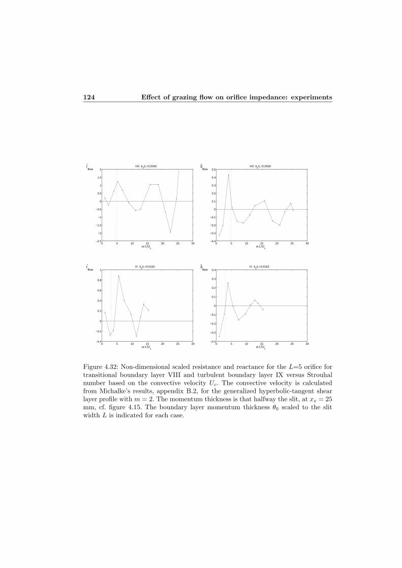
124 Effect of grazing flow on orifice impedance: experiments
0 5 10 15 20 25 30−2.5
−2
−1.5
−1
−0.5
0
0.5
1
1.5
2
ω L/Uc
~rflow
VIII θ
0/L=0.0058
0 5 10 15 20 25 30−0.4
−0.3
−0.2
−0.1
0
0.1
0.2
0.3
0.4
0.5
ω L/Uc
~δflow
VIII θ
0/L=0.0058
0 5 10 15 20 25 30−0.4
−0.2
0
0.2
0.4
0.6
0.8
1
ω L/Uc
~rflow
IX θ
0/L=0.0162
0 5 10 15 20 25 30−0.4
−0.3
−0.2
−0.1
0
0.1
0.2
0.3
0.4
ω L/Uc
~δflow
IX θ
0/L=0.0162
Figure 4.32: Non-dimensional scaled resistance and reactance for the L=5 orifice fortransitional boundary layer VIII and turbulent boundary layer IX versus Strouhalnumber based on the convective velocity Uc. The convective velocity is calculatedfrom Michalke’s results, appendix B.2, for the generalized hyperbolic-tangent shearlayer profile with m = 2. The momentum thickness is that halfway the slit, at xs = 25mm, cf. figure 4.15. The boundary layer momentum thickness θ0 scaled to the slitwidth L is indicated for each case.

4.7 Results 125
0 5 10 15−3
−2
−1
0
1
2
3
4
5
ω L/U0
~rflow
<|rflow
|> ~
0 5 10 15−6
−4
−2
0
2
4
ω L/U0
~δflow
~ <|δflow
|>
Figure 4.33: Non-dimensional scaled resistance and reactance for the L=5 orifice fortransitional boundary layer VIII (+ markers) and turbulent boundary layer IX (∗markers) versus Strouhal number based on the mean flow velocity U0: data of figure4.25. The resistance and reactance are scaled to the average of their absolute value.
0 5 10 15 20 25 30−3
−2
−1
0
1
2
3
4
ω L/Uc
~rflow
<|rflow
|> ~
0 5 10 15 20 25 30−4
−3
−2
−1
0
1
2
3
4
ω L/Uc
~δflow
~ <|δflow
|>
Figure 4.34: Non-dimensional scaled resistance and reactance for the L=5 orifice fortransitional boundary layer VIII (+ markers) and turbulent boundary layer IX (∗markers) versus Strouhal number based on the convective velocity Uc: data of figure4.32. The resistance and reactance are scaled to the average of their absolute value.

126 Effect of grazing flow on orifice impedance: experiments
observed can be made. From appendix B.2, in particular figure B.2, it follows thatfor a shear layer with generalized hyperbolic-tangent profile hydrodynamic instabilityoccurs up to a Strouhal number on the momentum thickness, ωθ/U0, less than about0.25. This value differs only slightly with profile parameter m. Using this, and theconcerning ratios of boundary layer momentum thickness θ0 (which is the minimummomentum thickness) to slit width L, the concerning maximum Strouhal numberωL/U0 is about 4.5, 5.4, 6.6, 8.6 and 3 for the 1 cm slot with boundary layer flows Ito V respectively. For the 5 cm slot the values are indeed much higher, namely 43 and15 for the boundary layer flows VIII respectively IX. The above mentioned numbersare fairly in agreement with what is observed in figures 4.30 and 4.33. It has to benoted that sandpaper tripped turbulent boundary layer flow V with the 1 cm slitseems to be a slight exception here, and for the 5 cm slot with transitional boundarylayer VIII measurements could not be performed at sufficient high Strouhal numberin order to assess where resistance and reactance due to the mean flow attenuate tozero.
4.7.6 Influence of edge geometry
The influence of the edge geometry of the orifice on the resistance and reactancedue to grazing flow is investigated for the L = 1 cm slot with turbulent boundarylayer flow V. The different edge geometries are as shown in figure 4.7. The slotswith asymmetrical edge geometries, fig.4.7b and c, are used both with the sharp edgeupstream and downstream. Results are given in figure 4.35. The edge geometry clearlyaffects the amplitudes of the oscillations in resistance and reactance. Compared to thedouble 90◦ edge geometry, the geometry with the single sharp 0◦ edge upstream givesnearly the same results. Results for the single sharp 27◦ edge upstream are also verysimilar regarding the reactance. For the resistance a more significant difference is seen,mostly in the region around a Strouhal number of 3, where it is positive, the resistanceis larger. Placing the sharp edges downstream has a larger effect, especially for the27◦ edge. The amplitudes of the oscillations in resistance are larger compared to boththe double 90◦ edge geometry and the corresponding geometries with the sharp edgeupstream. For the single sharp 0◦ edge downstream the reactance increases in theregion where it is positive. For the 27◦ edge also a significant effect on the reactanceis seen in the regions where it is negative. For the geometry with sharp 27◦ edges bothupstream and downstream a slightly further increase is seen in the amplitude of theoscillations. In conclusion, mainly the downstream edge geometry affects the orificeimpedance with grazing flow. The oscillations in non-dimensional scaled resistanceand reactance are found to increase when sharp edges are used compared to thenormal 90◦ edge geometry. The strongest effect is seen for the sharp 27◦ edges.

4.7 Results 127
0 0.5 1 1.5 2 2.5 3 3.5 4−3
−2
−1
0
1
2
3
4
ω L/U0
~rflow
0 0.5 1 1.5 2 2.5 3 3.5 4−1
−0.5
0
0.5
1
1.5
2
2.5
3
ω L/U0
~δflow
Figure 4.35: Non-dimensional scaled resistance and reactance for the L=1 orifice withdifferent edge geometries, cf. figure 4.7, in case of boundary layer flow V. × markers:90◦ edges both sides, ∗ markers: single sharp 27◦ edge upstream, + markers: singlesharp 27◦ edge downstream, ◦ markers: sharp 27◦ edges both sides, � markers: singlesharp 0◦ edge upstream, � markers: single sharp 0◦ edge downstream.

128 Effect of grazing flow on orifice impedance: experiments
4.8 Conclusion
The effect of grazing mean flow on the acoustical impedance of a rectangular orificeis investigated experimentally. For this purpose an impedance tube set-up with anaccurate multi-microphone technique is used.
Measurements are done for slots with different width L in the flow direction,viz. 1 cm and 5 cm. Furthermore, different boundary layer flows, both laminar andturbulent, are considered. In this context boundary layer characterization as well asshear layer profile measurements are carried out.
Both resistance and reactance due to the grazing flow display an oscillating be-haviour as function of Strouhal number on the orifice width. By using the phasevelocity Uc of the hydrodynamic instability, these oscillations are more or less foundat the same Strouhal numbers ωL/Uc for all configurations. On basis of the shearlayer profile measurements, this convective velocity is (roughly) calculated using datafor the generalized hyperbolic-tangent profile given in literature.
The presence of hydrodynamic instability, which is for given profile dependent onthe Strouhal number ωθ/U0 based on the shear layer momentum thickness θ and mainflow velocity outside the boundary layer/shear layer U0 , seems to govern the presenceof the oscillations in resistance and reactance. Above a certain Strouhal number thehydrodynamic instability as well as the oscillations vanish. Consequently, the ratio ofslot width to momentum thickness determines the number of oscillations seen.
For boundary layers with similar shape the amplitudes of the oscillations increasewith decreasing boundary layer thickness (for fixed aperture width). Furthermore, theonset of non-linearity seems to be at lower amplitudes within the regions of strongoscillations in impedance.
The influence of the edge geometry has been investigated for the 1 cm wide slot.The amplitudes of the oscillations in resistance and reactance due to the grazing flowwere observed to be larger for sharp edge geometries. Especially, the form of thedownstream edge is important.
Chapter 5
Grazing flow over an orifice:modal analysis
5.1 Introduction
In this chapter the effect of grazing flow on the acoustical properties of an orificein a wall will be modelled using modal analysis. First, the considered geometry andthe accompanying matching procedure to obtain a scattering matrix for this specificproblem will be given. Also the calculation of an orifice impedance from the scatteringmatrix will be treated.
First, as a test, calculations are done for the orifice geometry without any meanflow. Convergence of the model is treated and comparison with potential theory ismade for the scattering at the orifice and the singular behaviour of the acoustic fieldat the orifice’s edges.
Next, model calculations for a uniform grazing flow are presented. Also here, con-vergence of the model is investigated, and the behaviour of the acoustic field near theedges is addressed. Furthermore, results are compared with the theoretical predictionby Howe’ source model [47], appendix A. In particular attention is given here to theinfluence of the geometrical ratios in the orifice configuration.
Finally, the effect of non-uniform grazing flow on orifice impedance is modelled.Convergence is treated and influence of grazing flow boundary layer thickness is in-vestigated. Model results are compared to experimental data from chapter 4.
Also, for the configurations with mean grazing flow, the effect of calculating orificeimpedance from either a pressure difference or a one-sided pressure on the results fornon-dimensional scaled resistance and reactance is discussed.

130 Grazing flow over an orifice: modal analysis
5.2 Mode matching
The considered geometry is given in figure 5.1. Basically, it consists of two paralleltwo-dimensional rectangular ducts infinite in the x-direction with height h1 and h2
respectively. The lower one carries mean flow U(y), while in the upper duct the fluidis quiescent. The orifice is represented by an interconnection with length L betweenthe two ducts. The complete geometry is divided into five ducts indicated by theboxed numbers. The mean flow profile in duct 1 continues unaltered in the orificeregion duct 3, and subsequently in duct 4. The acoustic pressure and velocity in eachduct is determined as an expansion of eigenmodes, calculated according to chapter 2.Matching, i.e applying continuity of the relevant variables, at the interfaces betweenducts 1 and 2 and duct 3 as well as between ducts 4 and 5 and duct 3 gives theacoustical behaviour of the orifice geometry in the form of a scattering matrix.
The mode matching procedure is similar in most aspects to that for the areaexpansion in a duct. For the basics one is referred to section 3.2, where this hasbeen discussed extensively for different mean flow configurations, viz. non-uniformflow, uniform flow and non-uniform flow with slip. Here, only the mode matchingprocedure for non-uniform flow with slip will be dealt with explicitly, as it is the mostextensive one. For this flow configuration it namely contains all aspects of the non-uniform flow configuration as well as the application of the Kutta condition, which isalso relevant for uniform flow. An extension to uniform flow and non-uniform flow iseasily made.
Ducts 1 and 4 in figure 5.1 have height h1 and number of points in y-directionN1, ducts 2 and 5 have height h2 and number of points N2. Consequently, duct 3has height h3 = h1 + h2 with N3 = N1 + N2 points. In duct 1 eigenmodes and
�
�
� � � �
� �
� � �
�
�
� � �
� � �
� ; � �
� �
2
1
5
�
�
� � � �
� �
� � �
�
�
� � �
� � �
� ; � �
� �
2
1
5
Figure 5.1: Considered geometry for modelling the effect of grazing flow on the acousti-cal behaviour of an orifice by modal analysis. The orifice is represented by an intercon-nection between two parallel two-dimensional rectangular ducts infinite in x-direction.The lower duct carries mean grazing flow U(y).

5.2 Mode matching 131
wavenumbers are calculated according to section 2.2. N1 acoustic and N1 neutralhydrodynamic modes propagating (or decaying) in the +x-direction and N1 acousticmodes propagating or decaying in the −x-direction are found. In duct 2 mean flowis absent, the modes are solved according to section 2.4, equation (2.20) with Machnumber M0 = 0. Here, N2 acoustic modes propagating or decaying in either directionare found. Clearly, duct 4 is identical to duct 1, and duct 5 is identical to duct 2,concerning their eigenmodes and wavenumbers. In duct 3 the modes are determinedaccording to section 2.5. This gives N3 acoustic modes and N1 + 2 hydrodynamicmodes propagating in +x-direction and N3 acoustic modes propagating/decaying in−x-direction. Continuity of the non-dimensional pressure and velocity disturbance p∗resp. v∗, and continuity of q∗ = i ∂p∗
∂x∗, cf. appendix D, at the interfaces at x = 0 and
x = L as well as the Kutta condition at the upstream edge gives the following set ofequations:
Q+1 C+
1 + Q−1 C−
1
Q+2 C+
2 + Q−2 C−
2
= Q+3 C+
3 + Q−3 C−
3
} N1
} N2
V+1 C+
1 + V−1 C−
1 = V+3 C+
3 + V−3 C−
3 } N1
P+1 C+
1 + P−1 C−
1
P+2 C+
2 + P−2 C−
2
= P+3 C+
3 + P−3 C−
3
} N1
} N2
Q+1 C+
4 + Q−1 C−
4
Q+2 C+
5 + Q−2 C−
5
= Q+3 C+′
3 + Q−3 C−′
3
} N1
} N2(5.1)
V+1 C+
4 + V−1 C−
4 = V+3 C+′
3 + V−3 C−′
3 } N1
P+1 C+
4 + P−1 C−
4
P+2 C+
5 + P−2 C−
5
= P+3 C+′
3 + P−3 C−′
3
} N1
} N2
V+nfC
+3 + V−
nfC−3 = 0
V+nfk
+3 C+
3 + V−nfk
−3 C−
3 = 0
Here the columns of Q, V and P contain the modes for q∗, v∗ and p∗. A distinction in+x (right) running and −x (left) running modes is made by the additional superscripts+ and − respectively. The subscripts indicate the duct number, cf. figure 5.1. Sincethe matrices containing the modes for duct 4 and 5 are identical to those for duct1 respectively duct 2, they have subscripts 1 and 2. Vnf contains the modes for the

132 Grazing flow over an orifice: modal analysis
velocity disturbance at the no flow side of the interface between mean flow and stillfluid in duct 3. Matrix k3 contains the wavenumbers in duct 3 on the diagonal. Thevectors C contain the coefficients of the modes. The modes in duct 1, 2 and 3 aretaken with respect to x, such that the x-dependence of the acoustic disturbancesis exp(−ikx). The modes in duct 4 and 5 are taken with respect to x′ = x − L,thus acoustic disturbances have exp(−ikx′) as x-dependence. Consequently, in thematching between ducts 3 and ducts 4 and 5 the modes in duct 3 are shifted. Thisis accounted for in the coefficients for the modes in duct 3, and is reflected by theadditional accent in vectors C, cf. equation (5.1). In this context the following relationshold:
C+′3 = E+C+
3 , (5.2)
C−3 = E−C−′
3 .
Here, matrices E+ and E− contain the corresponding values of exp(−ik+3 L) respec-
tively exp(ik−3 L) on the diagonal. Equations (5.1) are written in a single matrix equa-tion: ⎛
⎜⎜⎜⎜⎜⎜⎜⎜⎜⎜⎜⎜⎜⎜⎜⎜⎜⎜⎝
−Q−1 0 0 0 Q+
3 Q−3 E−
0 −Q−2 0 0
−V−1 0 0 0 V+
3 V−3 E−
−P−1 0 0 0 P+
3 P−3 E−
0 −P−2 0 0
0 0 −Q+1 0 Q+
3 E+ Q−3
0 0 0 −Q+2
0 0 −V+1 0 V+
3 E+ V−3
0 0 −P+1 0 P+
3 E+ P−3
0 0 0 −P+2
0 0 0 0 V+nf −V−
nfE−
0 0 0 0 V+nfk
+3 −V−
nfk−3 E−
⎞⎟⎟⎟⎟⎟⎟⎟⎟⎟⎟⎟⎟⎟⎟⎟⎟⎟⎟⎠
︸ ︷︷ ︸S1
⎛⎜⎜⎜⎜⎜⎝
C−1
C−2
C+4
C+5
C+3
C−′3
⎞⎟⎟⎟⎟⎟⎠ =
⎛⎜⎜⎜⎜⎜⎜⎜⎜⎜⎜⎜⎜⎜⎜⎜⎜⎜⎜⎝
Q+1 0 0 0
0 Q+2 0 0
V+1 0 0 0
P+1 0 0 00 P+
2 0 00 0 Q−
1 00 0 0 Q−
2
0 0 V−1 0
0 0 P−1 0
0 0 0 P−2
0 0 0 00 0 0 0
⎞⎟⎟⎟⎟⎟⎟⎟⎟⎟⎟⎟⎟⎟⎟⎟⎟⎟⎟⎠
︸ ︷︷ ︸S2
⎛⎜⎝
C+1
C+2
C−4
C−5
⎞⎟⎠ . (5.3)
5.3 Calculation of the impedance 133
Here, matrix S1 is square with 6N1 + 4N2 + 2 rows and columns. matrix S2 is 6N1 +4N2+2 rows by 3N1+2N2 columns. The scattering matrix S is given by: S = S1
−1S2.It relates the coefficients of the modes propagating/decaying away from the orificeregion duct 3 as well as the coefficients of the modes in duct 3 to the coefficients ofthe modes propagating/decaying towards the orifice region:
⎛⎜⎜⎜⎜⎜⎜⎝
C−1
C−2
C+4
C+5
C+3
C−′3
⎞⎟⎟⎟⎟⎟⎟⎠
= S
⎛⎜⎜⎝
C+1
C+2
C−4
C−5
⎞⎟⎟⎠ . (5.4)
Note that in equation (5.3) the +x propagating / decaying acoustic modes in duct 3are counted from the left side, whereas the −x propagating / decaying acoustic modesare counted from the right side. This is reflected by the use of coefficient vectors C+
3
and C−′3 , and results in the use of the above defined matrices E+ and E−, which
account for the propagation/decaying of the corresponding modes in duct 3. Here, forthe evanescent acoustic modes, both E+ and E− contain exponentially small numbers.By doing so, the occurrence of both very large and very small numbers in rows andcolumns of matrix S1, possibly leading to difficulties in the inversion, is reduced. Ifnamely both the +x and −x propagating / decaying acoustic modes in duct 3 werecounted from, say, the left side, matrices would have to be used, analogous to E+ andE−, which contain exponentially small numbers for the +x decaying acoustic modesand exponentially large numbers for the −x decaying acoustic modes.
5.3 Calculation of the impedance
As in the previous chapter, the acoustical behaviour of the orifice with grazing flowwill be expressed in terms of an impedance. The impedance Zh of an orifice was givenby equation (4.3) for the low frequency limit. For the orifice geometry consideredhere, figure 5.1, the impedance can be calculated from the propagation of the planewaves. Figure 5.2 shows the geometry again, here also the Fourier transformed (thatis with the factor exp(iωt) dropped) plane wave acoustic pressures and velocities (inx-direction) in ducts 1 to 4 at the interface with the orifice region duct 3 are indicated.The plane wave pressure at these interfaces is just the sum of the pressure amplitude ofthe plane wave propagating to the right and the pressure amplitude of the plane wavepropagating to the left: p1 = p+
1 + p−1 etcetera. As an approximation the pressure p−at the no flow side, in this case above the orifice, is given by the average of pressuresp2 and p5. Similarly, the pressure p+ at the mean flow side, beneath the orifice, isgiven by the average of p1 and p4. The area averaged acoustic velocity uh through

134 Grazing flow over an orifice: modal analysis
the orifice is calculated by taking the volume in duct 3 above the orifice as a controlvolume to which continuity of mass is applied. In linearized form:
∂
∂t
∫∫∫V
ρ′dV +∫∫
S
ρ0(−→n · −→v ′)dS = 0, (5.5)
with ρ0 the mean mass density and ρ′ the acoustic density disturbance and v′ theacoustic velocity. With the harmonic time dependence exp(iωt) of the acoustic vari-ables, and with p′ = c20ρ
′, we have:
uh =h2
L(u2 − u5) − i
ωh2
ρ0c20p−. (5.6)
With u2 = (p+2 − p−2 )/ρ0c0 and u5 = (p+
5 − p−5 )/ρ0c0, see for example equation (4.9),and the non-dimensionalization employed with modal analysis, cf. equation (2.8), thisbecomes:
uh∗ =h2∗L∗
((p+
2∗ − p−2∗) − (p+5∗ − p−5∗)
)− iω∗h2∗p−∗. (5.7)
Duct height h1 is used here as characteristic length scale. All the quantities of interestare now expressed in the dimensionless pressures. In the modal analysis the amplitudesof the plane wave modes are normalized to unity. So for p+
1∗ and p−1∗ the coefficientC+
1 (1) respectively C−1 (1) can be used, etcetera. Furthermore, the impedance, given
�
�
� �
� � �
�
�
� � �
� � �
� ; � �
� �
2
1
5� �
� �
� 5
� 5
� �
� �
� 1
� 1
� �
�
�
� �
� � �
�
�
� � �
� � �
� ; � �
� �
2
1
5� �
� �
� 5
� 5
� �
� �
� 1
� 1
� �
Figure 5.2: Orifice geometry in the modal analysis method, also shown in figure 5.1.Here the relevant quantities for calculating the orifice impedance are indicated: p1,2,4,5
are the pressure disturbances due to the plane waves in ducts 1,2,4 and 5 respectivelyat the interface with orifice region duct 3, uh is the (area averaged) acoustic velocitythrough the orifice. uh is calculated from the acoustic velocities due to the plane wavesin duct 2 and 5 (no mean flow side of the orifice) at the interface with duct 3, wherealso the compressibility of the volume above the orifice is accounted for.

5.4 No mean flow 135
in equation (4.3), is expressed in non-dimensional variables:
Zh =p−∗ − p+∗
uh∗. (5.8)
Note that in the calculations of impedance a symmetric plane wave excitation abovethe orifice will be used. This means that plane waves propagating towards the orificeregion are imposed in ducts 2 and 5. In ducts 1 and 4 beneath the orifice, where meanflow is present, an anechoic condition is applied. This means that no modes propagatethere towards the orifice region.
5.4 No mean flow
First, as a test the results of the modal analysis method for the current orifice geometrywill be studied in case no mean flow is present. Convergence in the calculation of theimpedance without mean flow (a quantity which is used later on to calculate the non-dimensional scaled resistance and reactance due to mean flow) as well as convergenceof the modal expansions will first be treated. Subsequently, results of the currentmodel for the scattering at the orifice as well as the singular behaviour of the acousticdisturbances at the edges of the orifice will be compared to what is predicted bypotential theory.
5.4.1 Convergence
Calculation of the orifice impedance without grazing mean flow Zh0, according tosection 5.3, has been done in case dimensionless frequency is ωh1/c0 = 0.01 and ratioof duct heights and slit width is h1 = h2 = L for different numbers of points N1 induct 1. The relative error ∆Zh0 as function of the number of points N1 is shown infigure 5.3. Here, the relative error is defined as the relative difference between thevalue calculated with N1 points and with N1 = Nref points:
∆Zh0,N1 =∣∣∣Zh0,N1 − Zh0,Nref
Zh0,Nref
∣∣∣.In this case for the reference value: Nref = 200. The absolute value of the relativeerror in the orifice impedance approximately decreases as N−1.13
1 up to N1 = 60.Besides the convergence of the calculated orifice impedance, also the convergence
of the modal expansion in the orifice region duct 3, cf. figure 5.1, is of interest. For thesame configuration as above: ωh1/c0 = 0.01, h1 = h2 = L, with number of pointsN1 =N2 = 100, N3 = 200, figure 5.4 shows the absolute value of the coefficients C+
3 (n) ofthe acoustic modes propagating/decaying in the +x-direction (which are counted fromthe upstream edge of the orifice), and the absolute value of the coefficients C−′
3 (n)

136 Grazing flow over an orifice: modal analysis
of the acoustic modes propagating/decaying in the −x-direction (which are countedfrom the downstream edge of the orifice) as function of the index n of the modeson a log-log scale. Note that in order to obtain a useful comparison of the value ofthe coefficients, each corresponding mode (with index n) for the pressure disturbancePe,n is normalized such that:
1N3
i=N3∑i=1
|Pe,n(i)|2 = 1.
For both +x and −x propagating/decaying modes the coefficients approximately de-crease as n−1.7 above n = 1.
100
101
102
10−6
10−5
10−4
10−3
10−2
N1
∆ Zh0,N1
Figure 5.3: Convergence of calculated orifice impedance Zh0 without grazing meanflow. The relative error ∆Zh0,N1 in Zh0 with respect to a reference value is plottedversus number of points N1 in duct 1 on a log-log scale. Number of points usedfor calculation of reference value N1 = Nref = 200. Up to N1 = 60 the relativeerror decreases approximately as N−1.13
1 . Dimensionless frequency ωh1/c0 = 0.01,h1 = h2 = L.

5.4 No mean flow 137
100
101
102
10−20
10−15
10−10
10−5
100
n
|C3+(n)|
n
100
101
102
10−20
10−15
10−10
10−5
100
|C3−’(n)|
n
Figure 5.4: Absolute value of the coefficients C+3 (n) of the acoustic modes propagat-
ing/decaying in the +x-direction (which are counted from the upstream edge of theorifice), and the absolute value of the coefficients C−′
3 (n) of the acoustic modes prop-agating/decaying in the +x-direction (which are counted from the downstream edgeof the orifice) as function of the index n of the modes on a log-log scale in absenceof mean flow. Absolute value of the coefficients decreases as n−1.7. Dimensionless fre-quency ωh1/c0 = 0.01, h1 = h2 = L, number of discrete points N1 = N2 = 100,N3 = 200.

138 Grazing flow over an orifice: modal analysis
5.4.2 Comparison with potential theory
In case grazing mean flow is absent, the acoustic behaviour of the present orificegeometry can also be modelled with potential theory. For this purpose a conformalmapping of the geometry is employed, see for instance Morse and Feshbach [73] andMorse and Ingard [74]. First, the results for the scattering of plane waves at theorifice geometry obtained by the modal analysis method will be compared to what ispredicted by potential theory. Subsequently, the behaviour of the acoustic field closeto the edges of the orifice as obtained by modal analysis is compared to the singularbehaviour found in potential theory.
Scattering
The present orifice geometry is considered with duct heights h1 = h2 and ratio ofslit width to duct height L/h1 = 0.1271. In the modal analysis calculations numberof points is N1 = N2 = 100. In duct 2 and duct 5 plane waves are sent towards theorifice region duct 3, yielding a symmetric excitation. The ducts 1 and 4 beneath theorifice are anechoic, i.e. no acoustic waves here propagate towards the orifice region.Due to the symmetry of the configuration (there is no mean flow) the reflection coeffi-cient of the plane waves is R = C−
2 (1)/C+2 (1) = C+
5 (1)/C−5 (1), and the transmission
coefficient can be defined as T = C−1 (1)/C+
2 (1) = C+4 (1)/C−
5 (1). Results for the re-flection and transmission coefficient obtained by modal analysis are compared withthe results of potential theory in figure 5.5. Good correspondence is observed. Forhigher frequency the deviation between modal analysis results and potential theoryincreases, especially for the phases. This is expected as the potential theory is onlyvalid in the low frequency limit. Note that for the case without mean flow the scat-tering results obtained by the present discretized modal analysis are also comparedto results obtained by an analytical modal analysis model. Excellent agreement wasobserved.
Edge singularity
For non-viscous flow the acoustic velocity at the edges of the orifice goes to infinity. Inpotential theory the acoustic velocity v′ in the vicinity of an edge is proportional toone over the square root of the distance r from the edge: v′ ∝ r−
12 , yielding 1/v′2 ∝ r.
For the present orifice configuration a modal analysis calculation is performed fordimensionless frequency ωh1/c0 = 0.01, h1 = h2 = L, and number of points N1 = 100in case a symmetric excitation with plane waves is imposed (as above). The acousticvelocity in the y-direction, v∗ in dimensionless and discretized form, is obtained fromthe summation of the velocity modes V. These velocity modes are obtained from thesolved pressure modes P according to equation (2.15), where a Mach number equalto zero is substituted. The acoustic velocity at the left interface of orifice region duct3, i.e. at the x position of the left edge of the orifice, is plotted against position y∗, as

5.4 No mean flow 139
0 0.2 0.4 0.6 0.8 10
0.1
0.2
0.3
0.4
0.5
0.6
0.7
0.8
0.9
1|R|,|T|
ω/ωc
0 0.2 0.4 0.6 0.8 1−2
−1.5
−1
−0.5
0
0.5
1
1.5
2arg(R),arg(T) (rad)
ω/ωc
Figure 5.5: Absolute value and phase of the reflection coefficient R (∗ markers), andtransmission coefficient T (+ markers) calculated with modal analysis method com-pared to potential theory (corresponding solid lines). On the horizontal axis is theangular frequency divided by the cut-off angular frequency ωc of the first higherorder mode in duct 1 ( ωch1/c0 = π). Configuration: h1 = h2, L/h1 = 0.1271,N1 = N2 = 100.

140 Grazing flow over an orifice: modal analysis
0.8 0.85 0.9 0.95 1 1.05 1.1 1.15 1.20
0.1
0.2
0.3
0.4
0.5
0.6
0.7
0.8
0.9
11/|v
*|2
y*=y/h
1
Figure 5.6: Singular behaviour of (non-dimensional) acoustic velocity v∗ near the edgeof the orifice at y∗ = y/h1 = 1. In modal analysis calculations proportionality between1/|v∗|2 and the distance from the edge is found, consistent with potential theory.Configuration: dimensionless frequency ωh1/c0 = 0.01, h1 = h2 = L, N1 = 100.
1/|v∗|2 versus y∗ in figure 5.6. Note that the edge is at y∗ = y/h1 = 1. For the rightorifice edge the same result is obtained due to the symmetry of the configuration.Indeed, near the edge proportionality between 1/|v∗|2 and the distance from the edgeis found.
5.5 Uniform flow
For uniform grazing flow results of the modal analysis method can be compared tothose of the model of Howe, appendix A. The difference in geometry surroundingthe orifice, i.e. ducts versus free space respectively, is overcome by using the non-dimensional scaled resistance and reactance due to the mean flow, defined in equation(4.6). As shown these quantities are in fact derived as parameters independent on sur-rounding geometry on basis of Howe’s results for a rectangular slot. Besides comparingthe results of the two models, first the convergence of the modal analysis method, thebehaviour of the solution near the orifice’s edges and the formalism of calculating theimpedance (using pressure difference or one-sided pressure) will be addressed. Fur-

5.5 Uniform flow 141
thermore, attention will be given to the influence of the ratio of the duct heights andslit width in the currently used orifice geometry.
5.5.1 Convergence
The non-dimensional scaled resistance rflow and reactance δflow due to grazing meanflow is calculated as function of the number of discrete points in case the dimensionlessfrequency is ω∗ = ωh1/c0 = 0.01, and the duct heights h1 and h2 and slit width Lare equal: h1 = h2 = L. Figure 5.7 shows a log-log plot of the relative error ∆rflow
and ∆δflow as function of the number of points N1 in duct 1. Here, the relative errorin the non-dimensional scaled resistance is defined as:
∆rflow,N1 =∣∣∣ rflow,N1 − rflow,Nref
rflow,Nref
∣∣∣.with rflow,N1 the calculated value of rflow with N1 points, and rflow,Nref
the valuewith a reference number of points Nref . Here Nref = 200. For the error in the non-dimensional scaled reactance an analogous equation holds. For different Strouhalnumbers about the same convergence rate is seen in rflow and δflow. The relativeerror ∆rflow,N1 and ∆δflow,N1 decrease approximately as N−1.35
1 . Note that for someStrouhal numbers the relative error in rflow is quite large. This is caused by the factthat at these Strouhal numbers the value for rflow is close to zero.
Besides the convergence of the result for the non-dimensional scaled resistance andreactance also the convergence of the modal expansion in the orifice region duct 3, cf.figure 5.1, is investigated. For the same configuration as above, with ωh1/c0 = 0.01,h1 = h2 = L, N1 = N2 = 100, N3 = 200 and Strouhal number ωL/U0 = 3, figure5.8 shows the absolute value of the coefficients Cac+
3 (n) of the acoustic modes prop-agating/decaying in the +x-direction (which are counted from the upstream edge ofthe orifice), and the absolute value of the coefficients C−′
3 (n) of the acoustic modespropagating/decaying in the −x-direction (which are counted from the downstreamedge of the orifice) as function of the index n of the modes on a log-log scale. Notethe additional superscript ac here denoting the +x acoustic modes, since C+
3 alsocontains the coefficients for the +x propagating hydrodynamic modes. In both casesgood convergence is observed, above n = 1 the coefficients approximately decrease asn−3. Note that for the +x propagating/decaying acoustic modes the contribution ofthe modes with an uneven pressure distribution -these modes have even index n- isrelatively large compared to the contribution of the modes with even pressure distri-bution. For the −x propagating/decaying acoustic modes the opposite is observed.
5.5.2 Behaviour at the edges of the orifice
Also for partly uniform flow the acoustic velocity in y-direction at the edges of theorifice can be studied. Especially the behaviour at the downstream edge is interesting

142 Grazing flow over an orifice: modal analysis
101
102
0
5
10
10−4
10−2
100
102
∆ ~rflow,N
1
ω L/U0
N1
101
102
0
5
10
10−10
10−5
100
∆ ~δflow,N
1
ω L/U0
N1
Figure 5.7: Convergence of calculated non-dimensional scaled resistance and reac-tance, rflow resp. δflow, due to grazing uniform flow as function of Strouhal numberωL/U0. The relative error in rflow and δflow with respect to a reference value, i.e.∆rflow,N1 resp. ∆δflow,N1 , is plotted against number of points in duct 1, N1, on a log-log scale. Number of points used for calculation of reference value N1 = Nref = 200.Error decreases approximately as N−1.35
1 . Dimensionless frequency ωh1/c0 = 0.01,h1 = h2 = L.

5.5 Uniform flow 143
100
101
102
10−20
10−15
10−10
10−5
100
n
|C3ac+(n)|
n
100
101
102
10−12
10−10
10−8
10−6
10−4
10−2
100
102
|C3−’(n)|
n
Figure 5.8: Absolute value of the coefficients Cac+3 (n) of the acoustic modes propagat-
ing/decaying in the +x-direction (which are counted from the upstream edge of theorifice), and the absolute value of the coefficients C−′
3 (n) of the acoustic modes prop-agating/decaying in the −x-direction (which are counted from the downstream edgeof the orifice) as function of the index n of the modes on a log-log scale for uniformgrazing flow. The absolute value of the coefficients decreases as n−3 Dimensionlessfrequency ωh1/c0 = 0.01, h1 = h2 = L, number of discrete points N1 = N2 = 100,N3 = 200, Strouhal number ωL/U0 = 3.

144 Grazing flow over an orifice: modal analysis
as no condition is applied here, opposed to the upstream edge, where a Kutta conditionis explicitly applied. The acoustic velocity in the y-direction, v∗ in dimensionless anddiscretized form, is obtained from the summation of the velocity modes V. Thesevelocity modes are obtained from the solved pressure modes P according to equation(2.15), where for the no mean flow part a Mach number equal to zero is substituted.However, due to the discontinuity of the velocity over the infinitely thin shear layer,the values of the mode at the last point with flow, Nf = N1, and the first pointwithout mean flow, Nf + 1 = N1 + 1 are given by:
i(ω∗ −M0k∗)V(Nf ) = − dPdy∗
|Nf,
iω∗V(Nf + 1) = − dPdy∗
|Nf +1, (5.9)
with (see also e.g. eq.(2.29)):
dPdy∗
|Nf=
P(Nf ) − P(Nf − 1)2∆h∗
− i(ω∗ −M0k∗)Vflow
2,
dPdy∗
|Nf +1=P(Nf + 2) − P(Nf + 1)
2∆h∗− iω∗Vnoflow
2. (5.10)
Where Vflow and Vnoflow are the explicitly solved modes for the velocity disturbanceat the flow side respectively the no flow side of the interface between mean flow and nomean flow. For the configuration ωh1/c0 = 0.01, h1 = h2 = L and Strouhal numberωL/U0 = 3, the absolute value of the non-dimensional acoustic velocity disturbancev∗ at the x-position of the upstream edge as well as the x-position of the downstreamedge is plotted against position y∗ = y/h1 in figure 5.9. At the upstream edge, x∗ = 0,y∗ = 1, the acoustic velocity is indeed zero, both at the flow side and the no flow side,due to the imposed Kutta condition. Furthermore, no singular behaviour near theedge is seen. At the x-position of the downstream edge the acoustic velocity increasesrapidly when moving to the edge itself at x∗ = L∗, y∗ = 1, especially in the regionwithout flow. Note that here, at the interface between mean flow and no mean flow, anallowed discontinuity in velocity is seen. The results of the calculations with differentnumbers of discrete points N3 in duct 3 do not readily suggest a singularity at thedownstream edge (i.e. that the velocity tends to infinity). In that case namely a moresignificant difference between the results of the calculations with different numbers ofpoints would be expected close to the edge. In any case the behaviour of the acousticvelocity near the downstream edge differs from the v∗ ∝ r−
12 behaviour without mean
flow.
5.5.3 Influence of impedance definition
Here, the calculated orifice impedance, to be presented as the non-dimensional resis-tance and reactance due to the grazing mean flow, will be treated for uniform grazing

5.5 Uniform flow 145
0 0.5 1 1.5 20
0.5
1
1.5|v
*|
y*=y/h
1
mean flow no mean flow
(a) x∗ = 0, upstream edge
0 0.5 1 1.5 20
5
10
15
20
25
30
35
40|v
*|
y*=y/h
1
mean flow no mean flow
(b) x∗ = L∗, downstream edge
Figure 5.9: Absolute value of the non-dimensional acoustic velocity v∗ at the x-positionof the upstream edge respectively the downstream edge of the orifice. ∗ markers:calculation with N3 = 200 points, ◦ markers: calculation with N3 = 300 points. Thedashed vertical lines indicate the y∗ position of the edge, or the interface betweenmean flow and no mean flow. Configuration: dimensionless frequency ωh1/c0 = 0.01,h1 = h2 = L, Strouhal number ωL/U0 = 3.

146 Grazing flow over an orifice: modal analysis
flow (infinitely thin shear layer). The calculation of the orifice impedance is given insection 5.3. The most obvious way is to calculate the impedance from the pressuredifference over the orifice. In Howe’s model for the orifice impedance under uniformgrazing flow, appendix A, also the pressure difference is considered. Comparison be-tween modal analysis results and Howe’s results can thus readily be made.
However, in the experiments, cf. chapter 4, only the pressure at the no flow sideof the orifice can be measured. Consequently, the impedance is calculated from onlythe pressure at the no flow side. A justification is given there by arguing that theradiation pressure at the grazing flow side of the orifice is nearly independent of theflow. By subtracting the impedance without flow, as is done in calculating the non-dimensional scaled resistance and reactance, the pressure at the flow side of the orificecan therefore be eliminated.
In order to investigate any difference, calculation of the orifice impedance for uni-form grazing flow with the modal analysis method is compared in case the pressuredifference is used and in case the pressure at the no flow side of the orifice is used.Results are presented in figure 5.10. Clearly, a significant difference between the twoformalisms is seen. Especially for large Strouhal number the resistance seems to tendto minus infinity. The inconsistency here may be connected to the fact that the in-finitely thin shear layer is always unstable. The growth rate of the instability in theorifice increases proportionally to the Strouhal number. It is observed that this leadsto an ever increasing amplitude of the acoustic pressure and velocity field with increas-ing Strouhal number (when the amplitude of the pressure waves used as excitationremains constant). For large Strouhal number, the large amplitudes of the fields maylead to the difference between the two formalisms of calculating the impedance, andespecially the diverting behaviour of the resistance. Later on, it is actually seen thatfor non-uniform grazing flow, in which case the instability of the shear layer vanishesabove a certain Strouhal number, no significant difference is present between the twoways of calculating impedance. In the following modal analysis calculations for uni-form grazing flow, which wil be compared to Howe’s model, impedance is calculatedfrom the pressure difference over the orifice.
5.5.4 Incompressible limit
In order to compare with results from Howe’s model, which is an incompressible(low Helmholtz number, low Mach number) approach, also the approach of an in-compressible limit in the modal analysis method has to be ensured. For this purposecalculations are done for different values of the dimensionless frequency, i.e. Helmholtznumber, ω∗ = ωh1/c0. The ratio of the duct heights h1 and h2 and the slit width Lis kept constant at h1 = h2 = L. Furthermore, the number of points in the discretiza-tion of y in duct 1 respectively duct 2 is N1 = 100 and, consequently, N2 = 100.For each dimensionless frequency calculations are done without mean flow and withuniform mean flow in order to obtain the non-dimensional scaled resistance rflow
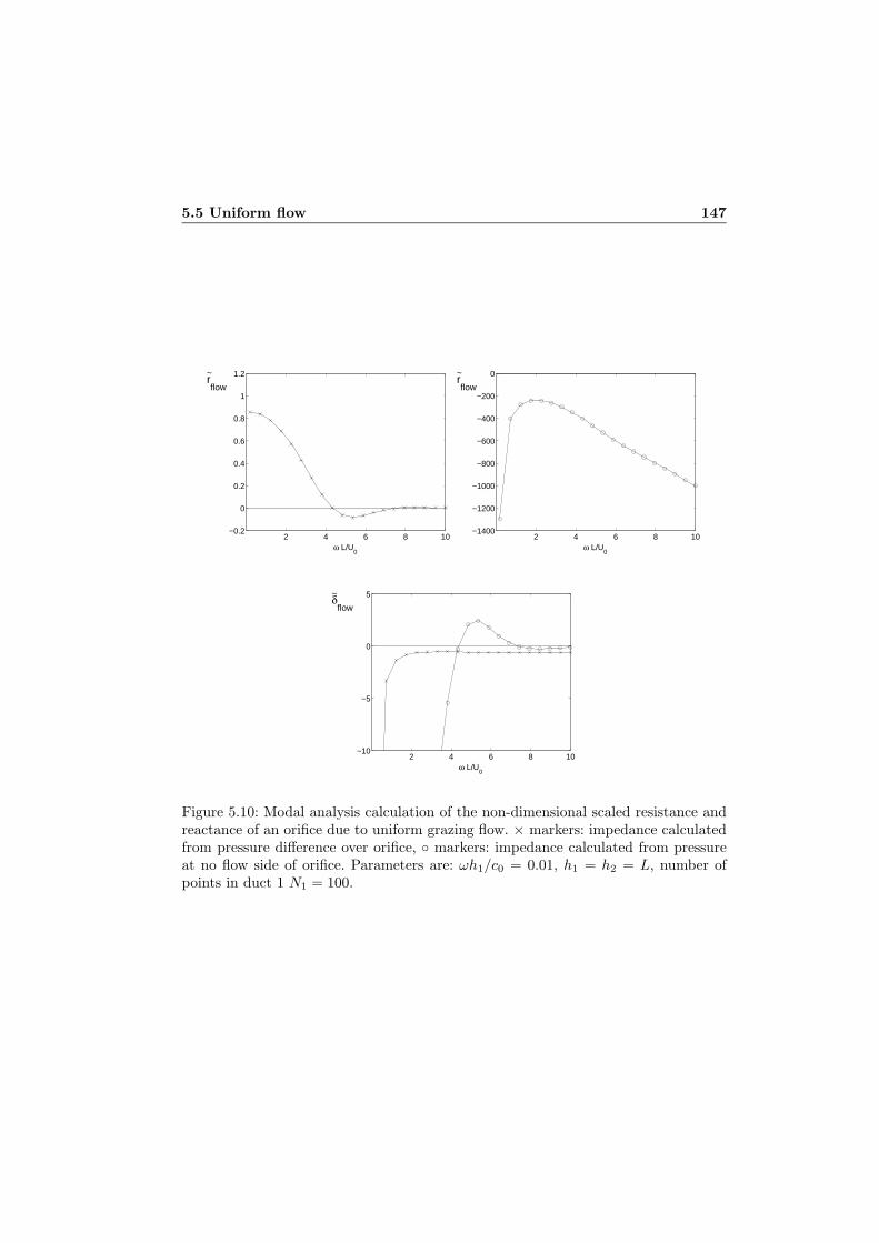
5.5 Uniform flow 147
2 4 6 8 10−0.2
0
0.2
0.4
0.6
0.8
1
1.2
ω L/U0
~rflow
2 4 6 8 10−1400
−1200
−1000
−800
−600
−400
−200
0
ω L/U0
~rflow
2 4 6 8 10−10
−5
0
5
ω L/U0
~δflow
Figure 5.10: Modal analysis calculation of the non-dimensional scaled resistance andreactance of an orifice due to uniform grazing flow. × markers: impedance calculatedfrom pressure difference over orifice, ◦ markers: impedance calculated from pressureat no flow side of orifice. Parameters are: ωh1/c0 = 0.01, h1 = h2 = L, number ofpoints in duct 1 N1 = 100.

148 Grazing flow over an orifice: modal analysis
and reactance δflow due to the flow. Calculations with mean flow at fixed dimension-less frequency are done at various Mach numbers. Results for rflow and δflow versusStrouhal number are shown in figure 5.11. At the lowest dimensionless frequency,ω∗ = 0.001, results seem to be converged fairly well to a low frequency limit. Theresults for resistance and reactance at dimensionless frequencies ω∗ = 0.1, ω∗ = 0.01and ω∗ = 0.001 are very close. Only for Strouhal number less than about 3 a differ-ence is seen between ω∗ = 0.1 and ω∗ = 0.001, which is at maximum about 5 percent.Between ω∗ = 0.01 and ω∗ = 0.001 only a slight difference of 1 percent at maximumis seen below Strouhal 1. Furthermore, the good correspondence of the resistance andreactance against Strouhal number for different frequencies, shows that these param-eters are indeed only a function of the Strouhal number as predicted by Howe’s model(when frequency is low enough and duct height to slit width ratio is fixed).
5.5.5 Influence of ratio of duct height and orifice width
Comparison of the modal analysis results with Howe’s model, appendix A, is madefor different ratios of duct heights h1, h2 to aperture width L in figure 5.12. Here,the dimensionless frequency is fixed. At given Strouhal number a lower dimensionlessfrequency yields a lower Mach number. At very low Mach numbers, which especiallyoccur for large h1/L ratios, problems in the calculations were encountered. Therefore,the dimensionless frequency is set at ω∗ = ωh1/c = 0.01. As discussed above thelow-frequency limit is well approached for this value. For the largest duct height toslit width ratio used, i.e. h1/L = 25, this yields a (still problem free) minimum Machnumber of M = 4 · 10−5 for Strouhal number ωL/U0 = 10. Furthermore, the ratio ofthe duct heights is fixed at unity: h1 = h2. Number of points in duct 1 is N1 = 100.Although the results of modal analysis calculations are qualitatively very similar tothose of Howe’s model, quantitatively they do not agree. Also a clear dependence onthe ratio of duct height to slit width is seen. This means that for the modal analysiscalculations the non-dimensional scaled resistance and reactance due to the flow areactually not independent on the geometry surrounding the orifice.

5.5 Uniform flow 149
0 1 2 3 4 5 6 7 8 9 10−0.1
0
0.1
0.2
0.3
0.4
0.5
0.6
0.7
0.8
0.9~rflow
ω L/U0
0 1 2 3 4 5 6 7 8 9 10
−1.2
−1
−0.8
−0.6
−0.4
−0.2
0
ω L/U0
~δflow
Figure 5.11: Non-dimensional scaled resistance rflow and reactance δflow due to theflow versus Strouhal number ωL/U0 calculated with modal analysis for different di-mensionless frequencies ω∗ = ωh1/c0. ◦ markers: ω∗ = 0.001, ∗ markers: ω∗ = 0.01,∇ markers: ω∗ = 0.1, + markers: ω∗ = 1. Ratio of duct heights and slit width ish1 = h2 = L. Number of points in duct 1 is N1 = 100.

150 Grazing flow over an orifice: modal analysis
0 1 2 3 4 5 6 7 8 9 10−1
−0.5
0
0.5
1
1.5
2
2.5
3
3.5
~rflow
ω L/U0
0 1 2 3 4 5 6 7 8 9 10−6
−5
−4
−3
−2
−1
0~δ
flow
ω L/U0
Figure 5.12: Non-dimensional scaled resistance rflow and reactance δflow due to theflow versus Strouhal number. Modal analysis calculation for different ratios of ductheights to slit width. × markers: h1/L = 1, + markers: h1/L = 5, ∗ markers: h1/L =25. Ratio of duct heights is unity: h1 = h2, dimensionless frequency ω∗ = ωh1/c0 =0.01. Number of points in duct 1 is N1 = 100. Thick solid lines without markers:results of Howe’s model, cf. appendix A.

5.6 Non-uniform flow 151
5.6 Non-uniform flow
In this section modal analysis results for the current orifice geometry with non-uniformgrazing flow are presented. First, the influence of impedance definition (i.e. calculatingit from a pressure difference or a one-sided pressure) and convergence of the methodare addressed. Subsequently, the influence of the boundary layer thickness of thegrazing flow on the acoustical behaviour of the orifice will be investigated. Somecomparison with experimental results from chapter 4 is made.
5.6.1 Influence of impedance definition
As already mentioned in section 5.5 about uniform grazing flow above, the orificeimpedance is most straightforwardly calculated from the pressure difference over theorifice. In experiments, cf. chapter 4, however only the pressure at the no flow sideof the orifice can be measured. Consequently, the impedance is calculated from onlythe pressure at the no flow side. A justification is given there by arguing that theradiation pressure at the grazing flow side of the orifice is nearly independent onthe flow. By subtracting the impedance without flow, as is done in calculating thenon-dimensional scaled resistance and reactance, the pressure at the flow side of theorifice can therefore be eliminated. Here, calculation of the orifice impedance with themodal analysis method for non-uniform grazing flow is compared in case the pressuredifference is used and in case the pressure at the no flow side of the orifice is used.The non-uniform flow profile function employed is given by:
f(y) =
⎧⎨⎩
1 − ( yh1
)m 0 ≤ y ≤ h1,
0 h1 < y ≤ h2,(5.11)
where the main flow velocity is given by U(y) = U0f(y). In this case U0 equals themaximum velocity, it is considered as the velocity outside the boundary layer. Themomentum thickness θ, relative to the orifice width L, for this profile is given by:
θ
L=
( 1m+ 1
− 12m+ 1
)h1
L. (5.12)
Figure 5.13 shows the non-dimensional scaled resistance rflow and reactance δflow
due to the grazing flow, cf. equation (4.6), as function of the Strouhal number ωL/U0,when using the pressure difference and when using the pressure at the no flow side only.The parameters in the calculation are: dimensionless frequency (Helmholtz number onduct height h1) ωh1/c0 = 0.05, duct heights h1 = h2, orifice width L = 0.2h1, numberof points in duct 1 N1 = 100, flow profile parameter m = 64 (θ/L = 0.038). Nearly thesame results are obtained when using pressure difference and pressure at the no flowside only. Note that this was also observed for all other calculations to be presented

152 Grazing flow over an orifice: modal analysis
2 4 6 8 10−3
−2
−1
0
1
2
3
4
ω L/U0
~rflow
stable unstable
0 2 4 6 8 10
−0.5
0
0.5
1
1.5
ω L/U0
~δflow
unstable stable
Figure 5.13: Modal analysis calculation of the non-dimensional scaled resistance andreactance of an orifice due to grazing flow. × markers: impedance calculated frompressure difference over orifice, ◦ markers: impedance calculated from pressure at noflow side of orifice. Parameters are: ωh1/c0 = 0.05, duct heights h1 = h2, orifice widthL = 0.2h1, number of points in duct 1 N1 = 100. Flow profile function is that givenby equation (5.11), with profile parameter m = 64.

5.6 Non-uniform flow 153
below. This result is very different from that obtained for uniform grazing flow. Inthat case namely a significant difference between the two ways of calculating theimpedance is seen. As discussed there, this may partly be connected to the fact thatfor uniform flow the growth rate of the shear layer instability increases proportionallywith the Strouhal number, giving ever increasing amplitudes of the acoustic fieldsfor an increasing Strouhal number. For non-uniform flow the shear layer instabilityvanishes above a certain Strouhal number, such that the amplitudes of the obtainedacoustical fields are limited.
Furthermore, the resistance and reactance calculated here show good resemblancewith experimental data, see chapter 4. In both cases similar oscillating behaviour isseen. In the graphs of figure 5.13 above, the Strouhal number, at which the shear layerbecomes stable, is indicated by the vertical dotted lines. Roughly the oscillations inresistance and reactance vanish at this point.
5.6.2 Convergence
The impedance for the configuration above has also been calculated for a numberof N1 = 50 and N1 = 150 points in duct 1. Corresponding results for the non-dimensional scaled resistance and reactance due to the flow, here derived from theimpedance calculated from the pressure difference over the orifice, are shown in fig-ure 5.14. Qualitatively the (oscillating) behaviour is similar for different numbers ofpoints. An exception is the non-dimensional scaled reactance δflow for N1 = 150.Compared to the calculations with N1 = 50 and N1 = 100 the positive peaks in δflow
radically change to an opposite negative value. The oscillations do not have the sameamplitude and are not at exactly the same Strouhal number for the different numbersof points. Thus the resistance and reactance do not converge for an increasing num-ber of points. For the resistance, however, convergence seems to be reasonably goodbelow a Strouhal number of about 1.5. Also at high Strouhal numbers, where theeffect of flow on impedance vanishes, convergence seems to be less problematic, this isespecially observed for the reactance. The above observed problems with convergenceof the method is also reported by Leroux [62], who applied a similar modal analysismodel in studying the propagation of acoustic waves in ducts with wall impedanceand non-uniform mean flow.
The data displayed in the graphs above is plotted again in figure 5.15, but asfunction of the Strouhal number based on the phase velocity Uc of the hydrodynamicinstability, instead of the velocity U0 outside the boundary layer. This phase veloc-ity of the hydrodynamic instability mode in the orifice region is calculated from itswavenumber according to equation (2.32). As a result the oscillations in resistanceand reactance are now found at virtually the same Strouhal number. Note that cal-culation of the Strouhal number based on the phase velocity of the hydrodynamicinstability mode can only be done when instability is present. At a certain Strouhal

154 Grazing flow over an orifice: modal analysis
0 2 4 6 8 10−5
−4
−3
−2
−1
0
1
2
3
4
ω L/U0
~rflow
0 2 4 6 8 10−3
−2.5
−2
−1.5
−1
−0.5
0
0.5
1
1.5
ω L/U0
~δflow
Figure 5.14: Modal analysis calculation of the non-dimensional scaled resistance andreactance of an orifice due to grazing flow versus Strouhal number ωL/U0 for differentnumbers of points. Impedance is calculated using the pressure difference over theorifice. + markers: N1 = 50, × markers: N1 = 100, ∗ markers: N1 = 150. Parametersare: ωh1/c0 = 0.05, duct heights h1 = h2, orifice width L = 0.2h1. Flow profilefunction is that given by equation (5.11), with profile parameter m = 64.

5.6 Non-uniform flow 155
0 5 10 15 20−5
−4
−3
−2
−1
0
1
2
3
4
ω L/Uc
~rflow
0 5 10 15 20−3
−2.5
−2
−1.5
−1
−0.5
0
0.5
1
1.5
ω L/Uc
~δflow
Figure 5.15: Modal analysis calculation of the non-dimensional scaled resistance andreactance of an orifice due to grazing flow versus Strouhal number ωL/Uc based onthe phase velocity of the hydrodynamic instability for different numbers of points.Impedance is calculated using the pressure difference over the orifice. + markers:N1 = 50, × markers: N1 = 100, ∗ markers: N1 = 150. Parameters are: ωh1/c0 = 0.05,duct heights h1 = h2, orifice width L = 0.2h1. Flow profile function is that given byequation (5.11), with profile parameter m = 64.

156 Grazing flow over an orifice: modal analysis
number in the plot of resistance and reactance, as displayed in figure 5.14, the hydro-dynamic instability vanishes. Therefore, only a part of the data in figure 5.14 reappearsin figure 5.15. Furthermore, comparing with experimental data for rflow and δflow
versus Strouhal number ωL/Uc for the 1 cm wide orifice, as displayed in figure 4.31,yields good agreement. The characteristic oscillations are observed at nearly the sameStrouhal numbers. Note here that the momentum thickness to slit width ratio for themodal analysis calculations is, using equation (5.12), θ/L = 0.038. This correspondsto the boundary layer flow III case in the experiments.
5.6.3 Influence of boundary layer thickness
Besides calculations for the above given configuration with flow profile parameterm = 64, yielding θ/L = 0.038, also calculations with profile parameter m = 53 areperformed. This gives a thicker boundary layer with θ/L = 0.046 (comparable tothe 1 cm slot with boundary layer flow II in experiments). Since no convergence inthe calculation of the impedance is obtained, the number of points taken in the twocases is such that the ratio of the momentum thickness θ and the spacing betweenthe points ∆h is equal. For m = 64 number of points is N1 = 100 as above, form = 53 number of points is N1 = 83. This gives θ/∆h = 0.76 for both cases. Resultsfor the non-dimensional scaled resistance and reactance versus Strouhal number onthe phase velocity of the hydrodynamic instability are plotted in figure 5.16. Theoscillations in resistance and reactance are virtually at the same Strouhal numberωL/Uc for the two cases with different boundary layer thickness. Note that this is notthe case when the Strouhal number ωL/U0 based on the mean flow velocity outside theboundary layer would be used. Furthermore, the amplitudes of the oscillations increasewith decreasing boundary layer thickness corresponding with what is observed inexperiments. Also, the amplitudes are of the same order as in experiments for thesecalculations. Note that for profile parameter m = 53 and m = 64 the ratio of shearlayer momentum thickness to duct height h3 is θ/h3 = 0.0046 and θ/h3 = 0.0038respectively. In chapter 2, section 2.7.2, it was shown for the hyperbolic-tangent shearlayer profile that for θ/h3 < 0.025 the hydrodynamic instability of the shear layercalculated with modal analysis in a duct geometry approached the result obtainedfor a shear layer which is unbounded in transverse direction. Therefore, for the abovecalculations the influence of the duct walls on the calculated hydrodynamic instabilityis supposed to be absent. Comparison with experiments, in which the shear layer isunbounded in the direction perpendicular to the mean flow, is thus justified in thatrespect.

5.6 Non-uniform flow 157
0 5 10 15−3
−2
−1
0
1
2
3
4
ω L/Uc
~rflow
0 5 10 15 20
−0.5
0
0.5
1
1.5
ω L/Uc
~δflow
Figure 5.16: Modal analysis calculation of the non-dimensional scaled resistance andreactance of an orifice due to non-uniform grazing flow versus Strouhal number ωL/Uc
based on the phase velocity of the hydrodynamic instability for different boundarylayer thicknesses. Flow profile function is that given by equation 5.11. + markers:m = 53, θ/L = 0.046, N1 = 83. ∗ markers: m = 64, θ/L = 0.038, N1 = 100. Ratioof momentum thickness to spacing between points equals θ/∆h = 0.76 in both cases.Other parameters are: ωh1/c0 = 0.05, duct heights h1 = h2, orifice width L = 0.2h1.Impedance is calculated using the pressure difference over the orifice.

158 Grazing flow over an orifice: modal analysis
5.7 Conclusion
In this chapter the modal analysis method has been applied to an orifice over whichgrazing mean flow is present. Here, the orifice is modelled as an interconnection be-tween two parallel ducts. The calculation of the orifice impedance for this geometryhas been treated.
Model calculations for the configuration in case mean grazing flow is absent showgood convergence. Furthermore, favourable comparison of results with the low fre-quency limit prediction by potential theory is shown for the scattering at the orificeand the singular behaviour of the acoustic field near the edges of the orifice.
For a uniform grazing mean flow also good numerical convergence of the method isfound. As expected, the behaviour of the acoustic field near the upstream edge is foundto be non-singular due to the application of the Kutta condition. At the downstreamedge the field seems to be non-singular, in any case different (singular) behaviour isfound than for the case in which mean flow is absent. A comparison is made betweenthe modal analysis results and the results of Howe’s incompressible source model,treated in appendix A. In the modal analysis method an incompressible limit is foundfor the non-dimensional scaled resistance and reactance due to the grazing flow, rflow
respectively δflow. As in Howe’s model, in this limit rflow and δflow only depend onthe Strouhal number. Qualitative, but not exact quantitative, agreement is observedbetween rflow and δflow as obtained by modal analysis (in the incompressible limit)and as predicted by Howe’s model. Moreover, the non-dimensional scaled resistanceand reactance due to the grazing flow calculated by modal analysis unexpectedlydepend on the ratio of duct height to slit width. Furthermore, they differ when calcu-lating the impedance either from the pressure difference over the orifice or from thepressure at the no flow side of the orifice only.
For non-uniform grazing flow numerical convergence of the modal analysis methodis not achieved at all Strouhal numbers. Results of calculations are therefore tenta-tively compared to experimental data of chapter 4, for fixed duct height to slit widthratio. It is found that the model’s results for the non-dimensional scaled resistanceand reactance due to the grazing flow are very similar to experimental results. In thecalculations the typical oscillations in resistance and reactance are virtually at thesame Strouhal number, based on the phase velocity of the hydrodynamic instabilityof the shear layer, for different numbers of discrete points. In this respect conver-gence of the method is established. However, generally no convergence is observedfor the amplitudes of these oscillations. An exception to this is the observed conver-gence in non-dimensional scaled resistance below a Strouhal number of about 1.5.Furthermore, in the high Strouhal number limit, where the oscillations vanish, con-vergence is established. The Strouhal numbers at which the oscillations are found inthe model calculations correspond very well to experimentally found values. For dif-ferent boundary layer thickness oscillations in the resistance and reactance are again
5.7 Conclusion 159
at the same Strouhal number, when it is based on the phase velocity of the hydrody-namic instability of the shear layer. When keeping the ratio of momentum thicknessto spacing between discrete points constant, the amplitude of the oscillations increasewith decreasing boundary layer thickness, which is consistent with experimental data.As opposed to the uniform flow case, for non-uniform grazing flow no significant dif-ference is observed for the non-dimensional scaled resistance and reactance due tothe flow when calculating the impedance either from the pressure difference over theorifice or from the pressure at the no flow side of the orifice.


Appendix A
Source model for orificeimpedance under uniformgrazing flow
Howe[45, 47] considered a two-sided grazing main flow U± in the x1-direction withinfinitesimally small boundary layer thickness (large Reynolds number) over an aper-ture in an infinitesimally thin wall, cf. figure A.1. The + and − subscripts refer tothe x2 > 0, respectively x2 < 0 region. In the aperture a shear layer develops, whichseparates the flows above and beneath the wall. Potential flow is assumed, except forthe infinitesimally thin region of the shear layer (vortex sheet), where all vorticity isconsidered to be concentrated. ϕ±(ω) and p±(ω) are the Fourier transformed velocitypotential respectively pressure for uniform linear perturbations taken at sufficientlylarge distance from the wall. Following Howe an e−iωt-convention is taken for theharmonic disturbances here, with ω the angular frequency. The pressure difference(p+ − p−)(ω) induces a flow through the aperture, corresponding to an additionalvelocity potential φ(x, ω), so that the total velocity potential of the perturbation is:
ϕ(x, ω) = ϕ±(ω) + φ(x, ω). (A.1)
Regarding the flow as locally incompressible: M2 = (U±c0
)2 � 1 andHe2 = (kL)2 � 1,with c0 the (mean) sound velocity, k = ω
c0the wavenumber and L the characteristic
size of the aperture, the velocity potential satisfies the Laplace equation:
∇2φ(x, ω) = 0. (A.2)
With the boundary condition for the flow velocity in the x2-direction, i.e. normal tothe wall: v2(x, ω) = 0 at x2 = 0 outside the aperture, the velocity potential is solved

162 Source model for orifice impedance under uniform grazing flow
U-
U+
p- , ϕ-
p+ , ϕ+
x1
x2
2s
U-
U+
p- , ϕ-
p+ , ϕ+
x1
x2
2s
b
x3
U-
U+
p- , ϕ-
p+ , ϕ+
x1
x2
2s
U-
U+
p- , ϕ-
p+ , ϕ+
x1
x2
2s
b
x3
Figure A.1: Two-sided grazing flow over an aperture.
with use of the Green’s function:
G(x,y, ω) =−1
4π|x − y| +−1
4π|x − y′| , y′ = (y1,−y2, y3), (A.3)
to obtain :
ϕ(x, ω) = ϕ±(ω) − sign(x2)2π
·∫ ∞
−∞
v2(y1,±0, y3, ω)|x − y| dy1dy3, y2 = 0, (A.4)
where the flow velocity in normal direction in the aperture v2(x1,±0, x3, ω) is un-known. By using the relations:
p(x, ω) = −ρ0(−iω + U±∂
∂x1)ϕ(x, ω), (A.5)
v2(x1,, 0, x3, ω) = (−iω + U±∂
∂x1)ζ(x1, x3, ω), (A.6)
with ρ0 the mean fluid density, this equation can be rewritten into a relation betweenthe pressure p(x, ω) and the normal displacement of the shear layer in the apertureζ(x1, x3, ω):
p(x, ω) = p±(ω) − ρ0sign(x2)2π
(ω + iU±∂
∂x1)2 ·
∫S
ζ(x1, x3, ω)|x − y| dy1dy3, y2 = 0,
(A.7)where the integration is now restricted to the area S of the aperture. This equationimplies that ζ(x1, x3, ω) is continuous over the vortex sheet (same value at x2 = ±0),which is reasonable in the infinitesimally thin wall case. However, recently Jing et al.[48] and Peat et al. [86] argued continuity of particle velocity rather than displacement

163
over the vortex sheet, whereas Auregan et al. [6, 8] concluded that an intermediateboundary condition between displacement and velocity continuity, depending on theboundary layer conditions, was most realistic to obtain a fit of the experimentalresults.
Finally, by demanding continuity of pressure over the aperture (at x2 = ±0), anequation for the shear layer displacement is found:
[(ω+iU+∂
∂x1)2+(ω+iU−
∂
∂x1)2]· 1
2π
∫S
ζ(x1, x3, ω)dy1dy3√(x′1 − y′1)2 + (x′3 − y′3)2
=p+ − p−ρ0
. (A.8)
After integration with respect to the differential operator on the left hand side wefind: ∫
S
ζ ′(y′1, y′3, ω)dy′1dy
′3√
(x′1 − y′1)2 + (x′3 − y′3)2+ λ1(x′3)e
iσ1x′1 + λ2(x′3)e
iσ2x′1 = 1, (A.9)
where the scaling:
ζ ′ =ρ0ω
2Lζ
π(p+ − p−), x′ =
x
L, y′ =
y
L,
is used to obtain a dimensionless form. Here L is the characteristic size of the aperturein streamwise direction. Furthermore:
σ1 =ωL(1 + i)U+ + iU−
= σ+1 + i1 + iµ
, σ2 =ωL(1 − i)U+ − iU−
= σ+1 − i1 − iµ
, (A.10)
are the dimensionless Kelvin-Helmholtz wave numbers of the instability waves of theshear layer, with σ+ = ωL
U+the Strouhal number based on velocity U+ and L, and
µ the ratio of flow velocities: µ = U−U+
. The terms on the left hand side of equation(A.9) with coefficients λ1 and λ2 represent the instability waves of the vortex sheet.For ω real: σ1 = σ∗
2 , so that one of the waves will grow exponentially in the x1-direction, which yields the instability. Note that equally strong grazing flow at bothsides: U− = U+ or µ = 1, gives σ1 = σ2 = σ+. The two terms in Eq. (A.9) are thenreplaced by: (λ1(x′3) + λ2(x′3)x
′1)e
iσ+x′1 . Since in this case σ+ is real, the motion of
the vortex sheet is stable.Equation (A.9) is (in general numerically) solved for the vortex sheet displacement
by applying the Kutta condition, ζ = ∂ζ∂x1
= 0, at the upstream edge. The shear layerthus leaves the upstream edge tangentially. Note that no condition is applied at thedownstream edge. With ζ found, the volume flux Q through the aperture can becalculated directly by:
Q(ω) =∫ ∞
−∞v2(x1, 0, x3, ω)dx1dx3 =
∫S
−iωζ(x1, x3, ω)dx1dx3, (A.11)

164 Source model for orifice impedance under uniform grazing flow
with use of equation (A.6). The acoustic behaviour of the aperture is then expressedin the Rayleigh conductivity KR defined as:
KR ≡ Q
ϕ+ − ϕ−= iωρ0
Q
p+ − p−. (A.12)
For a rectangular aperture with large aspect ratio, b � 2s, cf. figure A.1, an exactanalytical expression for the Rayleigh conductivity was found:
KR =πb
2(F (σ1, σ2) + Ψ), (A.13)
where σ1,2 are as defined in equation (A.10), and in this case are based on the half-width s of the slot (so L is replaced by s). The function F is given by:
F (σ1, σ2) =−σ1J0(σ2)G(σ1) + σ2J0(σ1)G(σ2)σ1W (σ2)G(σ1) − σ2W (σ1)G(σ2)
,
G(x) = J0(x) − 2W (x), W (x) = ix(J0(x) − iJ1(x)), (A.14)
with J0 and J1 Bessel functions of the first kind of zeroth and first order respectively.Ψ is related to the local approximations of the Green’s functions on either side of theaperture. For instance, for a three-dimensional free space on both sides:
Ψ±3D = ln(4bs
) − 1. (A.15)
Figure A.2 shows a plot of the Rayleigh conductivity of a slot with aspect ratio b2s = 10
for one-sided grazing flow, µ = 0, according to equation (A.13). Here the conductivity:
KR = 2Re(ΓR − i∆R), (A.16)
is scaled to the hydraulic radius of the aperture: Re =√
2sbπ . ΓR and ∆R correspond
to a reactance respectively resistance of the orifice, which according to the presenttheory thus only depend on the Strouhal number, for given aspect ratio and flowvelocity ratio µ. For ∆R > 0, Q is proportional to −(p+ − p−), cf. eqs. (A.12) and(A.16). The power P performed by the pressure load on the aperture flow equalsP = −(p+ − p−) · Q. So for ∆R > 0 the power is positive: P ∝ (p+ − p−)2 > 0.Energy is thus transferred from the pressure field to the aperture flow, which impliessound absorption. It can be seen in figure A.2 that sound absorption takes place forlow Strouhal numbers, ωs
U+< 1.6. For higher Strouhal numbers, 1.6 < ωs
U+< 3.5, ∆R
is negative, here sound production occurs.Grace et al. [37] computed the Rayleigh conductivity, according to the present
theory of Howe [47, 45], for 8 different shapes of wall apertures, such as a square and

165
0 1 2 3 4 5 6−1
−0.5
0
0.5
1
1.5
2
2.5
3
3.5
ωs/U+
KR
/Re
ΓR
∆R
Figure A.2: Scaled Rayleigh conductivity of a slot with aspect ratio b2s = 10 in a
infinitesimally thin wall for one-sided grazing flow, U− = 0, according to the theoryof Howe [47, 45].
a circle. It was found that, especially for one-sided grazing flow, KR is very similar tothat displayed in figure A.2 for all geometries.
Furthermore Howe investigated the influence of wall thickness d on the Rayleighconductivity [47, 46]. For a thin wall approximation, d
L � 1, and for the wavelengthsof disturbances on the vortex sheet large compared to d (σ+ � L
d ), the verticaldisplacement of fluid in the aperture was regarded independent on x2, and thus thesame as the vortex sheet displacement ζ(x1, x3, ω) at the upper and lower end of theaperture at x2 = ± 1
2d. Instead of demanding continuity of pressure over the vortexsheet, as in the infinitesimally thin wall case, now the pressure difference between theupper and lower end of the aperture can be set equal to the inertia −ρ0d
∂2ζ∂t2 = ρ0dω
2ζ.From equation (A.7) the equivalent of equation (A.8) is then deduced for a wall offinite thickness:
dω2ζ(x1, x3, ω) + [(ω + iU+∂
∂x1)2 + (ω + iU−
∂
∂x1)2]
· 12π
∫S
ζ(x1, x3, ω)dy1dy3√(x′1 − y′1)2 + (x′3 − y′3)2
=p+ − p−ρ0
. (A.17)
The Rayleigh conductivity of rectangular orifices was calculated for several thicknessesand for one-sided as well as even two-sided grazing flow [46]. It was argued that theintroduction of a finite wall thickness in all cases modifies the stability of the shearlayer motion (in the two-sided grazing flow case the motion also becomes unstable).

166 Source model for orifice impedance under uniform grazing flow
For one-sided grazing flow the Rayleigh conductivity was found to be very similarto the infinitely thin wall case. Especially the low Strouhal number region of soundabsorption remains nearly unaffected. For walls with d
L > 0.05 the region of soundproduction vanishes. It was however questioned, whether the thin wall approximationstill holds in this case.

Appendix B
Hydrodynamic (in)stability ofa free shear layer
B.1 Rayleigh’s equation
In case viscosity can be neglected the motion of a perfect and isentropic fluid isdescribed by the Euler equations for conservation of momentum and mass:
ρD−→vDt
= −−→∇p (B.1)
,1ρ
DρDt
= −−→∇ · −→v , (B.2)
DDt
=∂
∂t+ −→v · −→∇ .
With ρ the density, p the pressure and −→v the velocity vector. Considering smallperturbations in a two-dimensional flow, where the mean flow velocity U(y) is only afunction of y, linearization of the Euler equations can be employed. With ρ = ρ0 + ρ′,p = p0 + p′, where ρ′ << ρ0, and −→v = U(y)−→e x + u′−→e x + v′−→e y, with −→e x,
−→e y unitvectors in the x- and y-direction, gives, from equation (B.1), the linearized Eulerequations for momentum:
ρ0(∂u′
∂t+ U
∂u′
∂x+
dUdy
v′) = −∂p′
∂x, (B.3)
and:
ρ0(∂v′
∂t+ U
∂v′
∂x) = −∂p
′
∂y. (B.4)

168 Hydrodynamic (in)stability of a free shear layer
Regarding the flow as incompressible the velocity disturbance can be written as func-tion of a disturbance stream function ψ:
u′(x, y, t) =∂ψ(x, y, t)
∂y, v′(x, y, t) = −∂ψ(x, y, t)
∂x. (B.5)
If we take the following complex form for this stream function:
ψ(x, y, t) = φ(y)ei(ωt−kx), (B.6)
and subtract ∂∂y eq.(B.3) from ∂
∂xeq.(B.4), Rayleigh’s stability equation is obtained[93],[29]: (
U(y) − ω
k
)(d2φ(y)dy2
− k2φ(y))− d2U(y)
dy2φ(y) = 0. (B.7)
B.2 Instability for the generalized hyperbolic-tangentshear layer profile
Michalke [67, 68, 69] investigated the spatial instability of a free shear layer. Heconsidered a generalized hyperbolic-tangent velocity profile for the shear layer [68]:
U(y)U0
= 1 − (1 +memf(m) yθ )−1/m,
f(m) =∫ 1
0
1 − z
1 − zmdz, (B.8)
which has an inflexion point at y = 0. Here θ is the momentum thickness of the shearlayer:
θ =∫ ∞
−∞
U(y)U0
(1 − U(y)
U0
)dy. (B.9)
The quantity m is a profile parameter setting the steepness of the no flow (y ≤ 0)to flow (y ≥ 0) transition. This is illustrated by figure B.1, showing the shear layerprofile for different values of m. For m = ∞ the profile becomes:
U(y)U0
={
0 y ≤ 01 − e−0.5 y
θ y ≥ 0m = ∞.
For m = 1 the tanh profile is obtained as extensively studied in [67]:
U(y)U0
= 0.5(1 + tanh(0.5
y
θ)), m = 1. (B.10)
By solving Rayleigh’s equation (B.7), where the angular frequency ω is taken real,φ(y) as well as the corresponding complex wavenumbers k of the hydrodynamic wave

B.2 The generalized hyperbolic-tangent shear layer profile 169
−6 −4 −2 0 2 4 60
0.2
0.4
0.6
0.8
1.0
y/θ
U(y)/U0
m=1
m=2
m=6
m=16
m=∞
m=34
Figure B.1: Generalized hyperbolic-tangent shear layer flow profiles as given by equa-tion (B.8) for different values of m.
is obtained. Note that if some φ(y) with wavenumber k is a solution, also its complexconjugate φ∗(y) with corresponding complex conjugate k∗ is a solution. Figure B.2shows the results for the real and imaginary part of k for different values of the profileparameter as obtained by Michalke. For the m = 1 case the results were experimen-tally confirmed by Freymuth [32] for low frequencies. The real part of k governs thephase velocity Uc of the wave according to: Uc = ω/(k). The phase velocity cal-culated from the data of k is given in figure B.3. The imaginary part of k gives thegrowth rate of the instability. In case the imaginary part of the wavenumber is nonzeroan exponentially growing and an ’opposite’ exponentially decaying hydrodynamic isfound. It can be seen that for about ωθ
U0< 0.07 the value of the wave number k (both
real and imaginary part) is independent of the shear layer profile parameter m.
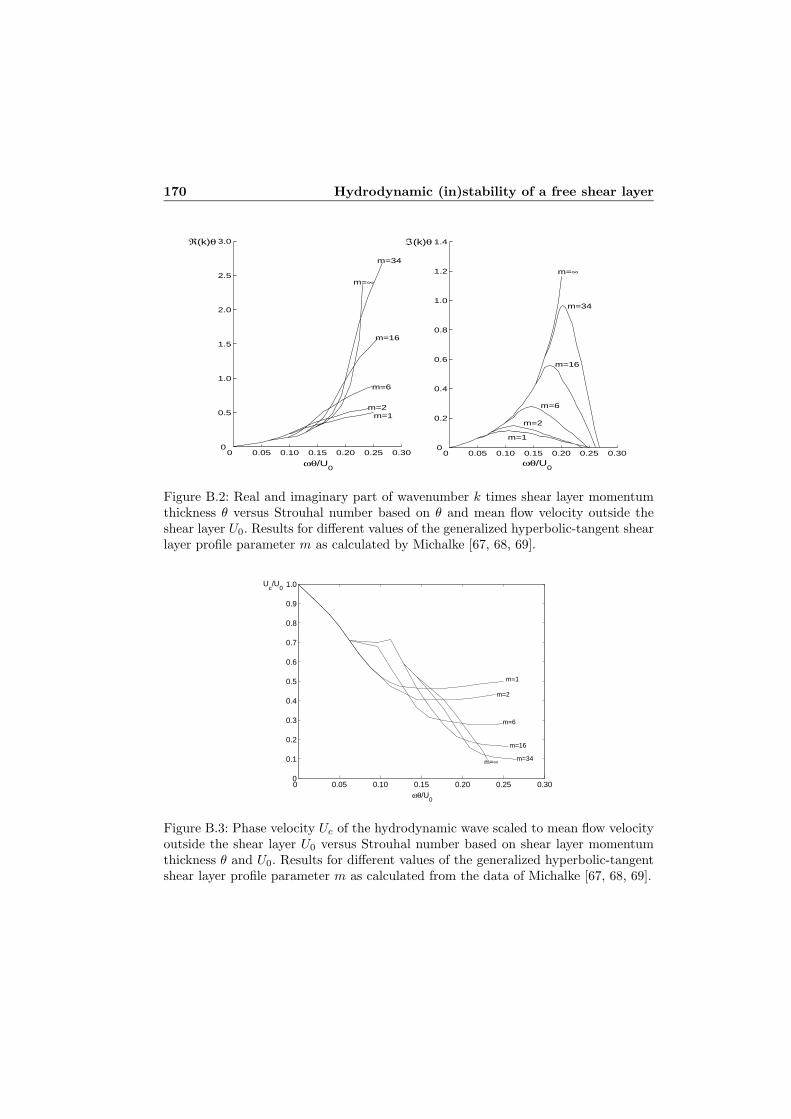
170 Hydrodynamic (in)stability of a free shear layer
0 0.05 0.10 0.15 0.20 0.25 0.300
0.5
1.0
1.5
2.0
2.5
3.0
0 0.05 0.10 0.15 0.20 0.25 0.300
0.2
0.4
0.6
0.8
1.0
1.2
1.4
m=∞
m=34
m=16
m=6
m=2 m=1
ωθ/U0
ℜ(k)θ
m=∞
m=34
m=16
m=6
m=2
m=1
ℑ(k)θ
ωθ/U0
Figure B.2: Real and imaginary part of wavenumber k times shear layer momentumthickness θ versus Strouhal number based on θ and mean flow velocity outside theshear layer U0. Results for different values of the generalized hyperbolic-tangent shearlayer profile parameter m as calculated by Michalke [67, 68, 69].
0 0.05 0.10 0.15 0.20 0.25 0.300
0.1
0.2
0.3
0.4
0.5
0.6
0.7
0.8
0.9
1.0
ωθ/U0
Uc/U
0
m=1
m=2
m=6
m=16
m=34 m=∞
Figure B.3: Phase velocity Uc of the hydrodynamic wave scaled to mean flow velocityoutside the shear layer U0 versus Strouhal number based on shear layer momentumthickness θ and U0. Results for different values of the generalized hyperbolic-tangentshear layer profile parameter m as calculated from the data of Michalke [67, 68, 69].

Appendix C
Differential matrices
Discrete derivatives
Consider a Taylor series expansion of a function f(y) around y = y0:
f(y0 + ∆y) =∞∑
n=0
1n!
dnf(y)dyn
|y=y0(∆y)n. (C.1)
Discretization of y in points with spacing ∆h gives the discrete form:
fn+∆n = fn + f ′n∆n∆h+12f ′′n (∆n∆h)2 +
16f ′′′n (∆n∆h)3 + ... , (C.2)
where the subscripts indicate the index of the discrete point. A prime denotes the firstderivative, double prime the second derivative, and so on. With the equation abovethe first and second derivative of f at discrete point n can be derived for differentorders of accuracy:
f ′n =−fn−1 + fn+1
2∆h+O((∆h)2),
f ′′n =fn−1 − 2fn + fn+1
(∆h)2+O((∆h)2), (C.3)
f ′n =fn−2 − 8fn−1 + 8fn+1 − fn+2
12∆h+O((∆h)4),
f ′′n =−fn−2 + 16fn−1 − 30fn + 16fn+1 − fn+2
12(∆h)2+O((∆h)4), (C.4)

172 Differential matrices
f ′n =−fn−3 + 9fn−2 − 45fn−1 + 45fn+1 − 9fn+2 + fn+3
60∆h+O((∆h)6),
f ′′n =2fn−3 − 27fn−2 + 270fn−1 − 490fn + 270fn+1 − 27fn+2 + 2fn+3
180(∆h)2+O((∆h)6).
(C.5)
Boundary condition
In the modal analysis the domain of y is restricted to a duct with walls at y = 0and y = h. Variables are discretized at N points in the y-direction. The points havespacing ∆h = N/h, while the first and last point are a distance ∆h/2 from the wall,cf. section 2.2. At the walls the first derivative of pressure w.r.t. y equals 0. Thisboundary condition can be incorporated by adding ghost points outside the duct, seefigure C.1. Equations for the first derivative of f(y) at the walls, y = 0 and y = h, asa function of the value of f at the surrounding (ghost) points can be derived, similarto equations (C.3, C.4, C.5). From those equations it is clear that the values of fat the discrete points around the position, where the first derivative is considered,appear asymmetrically. This means that by taking f−1 = f1, f−2 = f2 etcetera, andfN+1 = fN , fN+2 = fN−1 etcetera, the first derivative of f at the walls will be zero.
�
� �
� �
�
�
� �
�
� �
� � ) �� � �
� � �
�
� �
� �
�
�
� �
�
� �
� � ) �� � �
� � �
Figure C.1: Introduction of ghost points at the duct walls when employing discretiza-tion of the y-coordinate in order to incorporate the boundary conditions in the dif-ferential matrices.
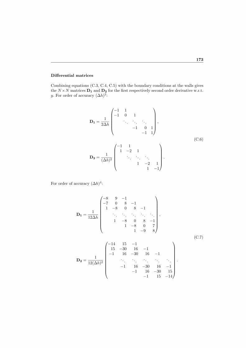
173
Differential matrices
Combining equations (C.3, C.4, C.5) with the boundary conditions at the walls givesthe N×N matrices D1 and D2 for the first respectively second order derivative w.r.t.y. For order of accuracy (∆h)2:
D1 =1
2∆h
⎛⎜⎜⎜⎜⎜⎝
−1 1−1 0 1
. . . . . . . . .−1 0 1
−1 1
⎞⎟⎟⎟⎟⎟⎠ ,
(C.6)
D2 =1
(∆h)2
⎛⎜⎜⎜⎜⎜⎝
−1 11 −2 1
. . . . . . . . .1 −2 1
1 −1
⎞⎟⎟⎟⎟⎟⎠ .
For order of accuracy (∆h)4:
D1 =1
12∆h
⎛⎜⎜⎜⎜⎜⎜⎜⎜⎜⎝
−8 9 −1−7 0 8 −1
1 −8 0 8 −1. . . . . . . . . . . . . . .1 −8 0 8 −1
1 −8 0 71 −9 8
⎞⎟⎟⎟⎟⎟⎟⎟⎟⎟⎠,
(C.7)
D2 =1
12(∆h)2
⎛⎜⎜⎜⎜⎜⎜⎜⎜⎜⎝
−14 15 −115 −30 16 −1−1 16 −30 16 −1
. . . . . . . . . . . . . . .−1 16 −30 16 −1
−1 16 −30 15−1 15 −14
⎞⎟⎟⎟⎟⎟⎟⎟⎟⎟⎠.
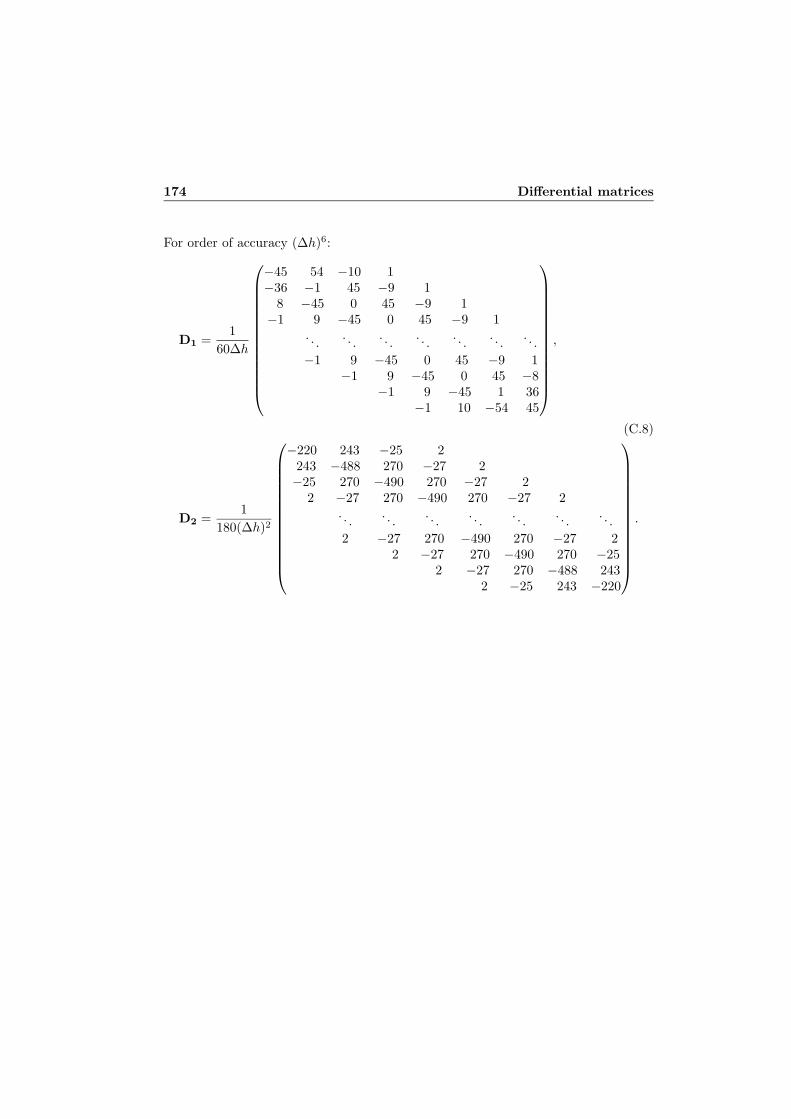
174 Differential matrices
For order of accuracy (∆h)6:
D1 =1
60∆h
⎛⎜⎜⎜⎜⎜⎜⎜⎜⎜⎜⎜⎜⎜⎝
−45 54 −10 1−36 −1 45 −9 1
8 −45 0 45 −9 1−1 9 −45 0 45 −9 1
. . . . . . . . . . . . . . . . . . . . .−1 9 −45 0 45 −9 1
−1 9 −45 0 45 −8−1 9 −45 1 36
−1 10 −54 45
⎞⎟⎟⎟⎟⎟⎟⎟⎟⎟⎟⎟⎟⎟⎠
,
(C.8)
D2 =1
180(∆h)2
⎛⎜⎜⎜⎜⎜⎜⎜⎜⎜⎜⎜⎜⎜⎝
−220 243 −25 2243 −488 270 −27 2−25 270 −490 270 −27 2
2 −27 270 −490 270 −27 2. . . . . . . . . . . . . . . . . . . . .2 −27 270 −490 270 −27 2
2 −27 270 −490 270 −252 −27 270 −488 243
2 −25 243 −220
⎞⎟⎟⎟⎟⎟⎟⎟⎟⎟⎟⎟⎟⎟⎠
.
Appendix D
Continuity conditions modematching
Consider a control volume around the interface between two ducts indicated 1 and 2.The integral equations for conservation of mass and momentum are:
∫∫S
ρ(−→n · −→v )dS = 0, (D.1)
and: ∫∫S
ρ−→v (−→n · −→v )dS +∫∫
S
p−→n dS = 0. (D.2)
Linearization:
p1 = p0 + p′1,ρ1 = ρ0 + ρ′1,−→v 1 = (u0 + u′1)
−→e x + v′1−→e y, (D.3)
p2 = p0 + p′2,ρ2 = ρ0 + ρ′2,−→v 2 = (u0 + u′2)
−→e x + v′2−→e y
gives:ρ0u
′1 + u0ρ
′1 = ρ0u
′2 + u0ρ
′2 (D.4)
for mass conservation, and:
u20ρ
′1 + 2ρ0u0u
′1 + p′1 = u2
0ρ′2 + 2ρ0u0u
′2 + p′2, (D.5)

176 Continuity conditions mode matching
respectively:v′1 = v′2 (D.6)
for momentum conservation in the x- and y-direction. Equation (D.5) can be rewrittenas:
(ρ0u′1 + u0ρ
′1)u0 + ρ0u0u
′1 + p′1 = (ρ0u
′2 + u0ρ
′2)u0 + ρ0u0u
′2 + p′2. (D.7)
Subsequently, subtracting u0 times equation (D.4) and substituting p′ = c20ρ′ gives:
ρ0u0u′1 + c20ρ
′1 = ρ0u0u
′2 + c20ρ
′2. (D.8)
Dividing equation (D.4) by ρ0 and subtraction u0/(ρ0c20) times equation (D.8) yields:
u′1(1 −M20 ) = u′2(1 −M2
0 ), (D.9)
with M0 = u0/c0. Consequently we have:
u′1 = u′2. (D.10)
Substituting this in the linearized conservation equations (D.4,D.5) returns:
ρ′1 = ρ′2, (D.11)
and:p′1 = p′2. (D.12)
The continuity of velocity disturbances u′ and v′ also implies the continuity of thederivative w.r.t. x of the pressure disturbance ∂p′/∂x, using equation (2.4) and thefact that the derivative of the mean flow, dU/dy, is continuous. The above yieldscontinuity of dimensionless parameters p∗, v∗ and u∗, cf. equation (2.8), and from thedefinition given in equation (2.12) continuity of q∗. In the mode matching procedurethe continuity of q∗, v∗ and p∗ is utilized.

Appendix E
Modal analysis in 2Dcylindrical geometry
In Chapter 2 the method of finding eigenmodes and accompanying wavenumbers forthe linear pressure and velocity disturbance in a two-dimensional rectangular ductis presented. Here, the method is extended to a two-dimensional cylindrical duct.We start from the same equations for a perfect and isentropic fluid, given by eqs.(2.1) through (2.3). Quantities are generally now a function of spatial coordinates xand radius r and time t. Any dependence on the angular coordinate is left out ofconsideration. Linearization then gives analogous to equations (2.4) through (2.6):
ρ0
( ∂∂t
+ U∂
∂x
)u′ + ρ0
dUdr
v′ = −∂p′
∂x, (E.1)
ρ0
( ∂∂t
+ U∂
∂x
)v′ = −∂p
′
∂r, (E.2)
1ρ0c20
( ∂∂t
+ U∂
∂x
)p′ = −
(∂u′∂x
+∂v′
∂r+v′
r
). (E.3)
Here u′ and v′ are the velocity disturbance in x- and r-direction respectively. Themean flow U is a function of r only. Note here that in cylindrical coordinates (r, θ, x)the divergence of a vector −→a is given by:
−→∇ · −→a =1r
∂rar
∂r+
1r
∂aθ
∂θ+∂ax
∂x.
Similar to equation (2.7) we can derive from these equations:
1c20
( ∂∂t
+ U∂
∂x
)2
p′ −(∂2p′
∂x2+∂2p′
∂r2+
1r
∂p′
∂r
)= 2ρ0
dUdr
∂v′
∂x. (E.4)

178 Modal analysis in 2D cylindrical geometry
Non-dimensionalization according to:
p∗ =1
ρ0c20p′, (x∗, r∗) = (
x
R,r
R),
(u∗, v∗) =1c0
(u′, v′), ω∗ =ωR
c0,
M(r) = M0f(r) =1c0U(r), t∗ =
c0t
R,
(E.5)
with R the duct radius, gives the non-dimensional form of equations (E.2,E.3):( ∂
∂t∗+M0f
∂
∂x∗
)v∗ = −∂p∗
∂r∗, (E.6)
( ∂
∂t∗+M0f
∂
∂x∗
)2
p∗ −( ∂2
∂x2∗+
∂2
∂r2∗+
1r∗
∂
∂r∗
)p∗ = 2M0
dfdr∗
∂v∗∂x∗
, (E.7)
analogous to equations (2.9) and (2.10). Writing the complex form:
p∗ = P (r∗)exp(−ik∗x∗)exp(iω∗t∗),v∗ = V (r∗)exp(−ik∗x∗)exp(iω∗t∗), (E.8)q∗ = Q(r∗)exp(−ik∗x∗)exp(iω∗t∗),
where q∗ = i∂p∗/∂x∗, leads to:
i(ω∗ −M0fk∗)V = − dPdr∗
, (E.9)
(1 −M20 f
2)k2∗P + 2ω∗M0fk∗P − ω2
∗P − d2P
dr2∗− 1r∗
dPdr∗
= −2iM0dfdr∗
k∗V. (E.10)
Subsequently, by discretization of r∗ the generalized eigenvalue problem analogous toequation (2.17) is found:
k∗
⎛⎝ I −M2
0 f2 2iM0fa 00 iM0f 00 0 I
⎞⎠⎛⎝ Q
VP
⎞⎠ =
⎛⎝ −2ω∗M0f 0 ω2
∗I + D2 + r−1∗ D1
0 iω∗I D1
I 0 0
⎞⎠⎛⎝ Q
VP
⎞⎠ . (E.11)
Here, matrix r−1∗ D1 represents the discretization of 1
r∗dPdr∗
. The matrices D1 and D2
give the first respectively second derivative with respect to r∗. They are identical tothe matrices for the first and second derivative with respect to y∗ used with cartesiancoordinates (Appendix C), since also here the boundary condition at r∗ = 0 andr∗ = R is dP/dr∗ = 0. For more specific flow configurations, the generalized eigenvalueproblem has to be adapted analogous to what is explained in sections 2.3, 2.4 or 2.5.

Bibliography
[1] M. Abom, H. Boden; Error analysis of two-microphone measurements in ductswith flow; J. Acoust. Soc. Am, vol. 83, pp. 2429-2438, 1988.
[2] N.K. Agarwal, M.K. Bull; Acoustic wave propagation in a pipe with fully de-veloped turbulent flow; J. Sound & Vibr., vol. 132(2), pp. 275-298, 1989.
[3] R.J. Alfredson, P.O.A.L. Davies; Performance of exhaust silencer components;J. Sound & Vibr., vol. 15(2), pp. 175-196, 1971.
[4] S. Allam, M. Abom; Investigation of damping and radiation using full planewave decomposition in ducts; J. Sound & Vibr., vol. 292, pp. 519-534, 2006.
[5] Y. Auregan; Comportement aero-acoustique basse-frequence d’une expansion;14eme Congres Francais de Mecanique, no. 451, Toulouse 1999.
[6] Y. Auregan, R. Starobinski, V. Pagneux; Influence of grazing flow and dissipa-tion effects on the acoustic boundary conditions at a lined wall; J. Acoust. Soc.Am, vol. 109(1), pp. 59-64, 2001.
[7] Y. Auregan, A. Debray, R. Starobinski; Low frequency sound propagation in acoaxial cylindrical duct: application to sudden area expansions and to dissipativesilencers; J. Sound & Vibr., vol. 243(3), pp. 461-473, 2001.
[8] Y. Auregan, M. Leroux; Failures in the discrete models for flow duct with per-forations: an experimental investigation; J. Sound & Vibr., vol. 265(1), pp. 109-121, 2003.
[9] Y. Auregan, M. Leroux, V. Pagneux; Measurement of liner impedance withflow by an inverse method; 10th AIAA/CEAS Aeroacoustics conference, AIAA2004-2838, 2004.
[10] P. Banks-Lee, H. Peng; Length error analysis for impedance tube measurements;J. Acoust. Soc. Am, vol. 85(4), pp. 1769-1772, 1989.

180 BIBLIOGRAPHY
[11] G.K. Batchelor; An introduction to fluid dynamics; Cambridge University Press,1970; ISBN 0-521-09817-3.
[12] A. Bers; Space-time evolution of plasma instabilities - absolute and convective.in: Handbook of plasma physics: volume 1 basic plasma physics, edited by A.A.Galeev and R.N. Sudan; North-Holland Publishing Company., 1983; ISBN 0-444-86645-0.
[13] A. Bihhadi, Y. Gervais; Propagation in duct with mean flow and temperaturegradients; Acta Acoustica, vol. 2 pp. 343-357, 1994.
[14] C.P.A. Blom; Discontinuous Galerkin method on tetrahedral elements for aeroa-coustics; PhD thesis, Universiteit Twente, NL, 2003.
[15] H. Boden, M. Abom; Influence of errors on the two-microphone method formeasuring acoustic properties in ducts; J. Acoust. Soc. Am, vol. 79(2), pp. 541-549, 1986.
[16] S. Boij, B. Nilsson; Reflection of sound at area expansions in a flow duct; J.Sound & Vibr., vol. 260(3), pp. 477-498, 2003.
[17] S. Boij, B. Nilsson; Scattering and absorption of sound at flow duct expansions;J. Sound & Vibr., vol. 289(3), pp. 577-594, 2006.
[18] R.J. Briggs; Electron-stream interaction with plasmas; MIT Press, 1964.
[19] A.M. Cargill; Low frequency acoustic radiation from a jet pipe - a second ordertheory; J. Sound & Vibr., vol. 83(3), pp. 339-354, 1982.
[20] W. T. Chu; Further experimental studies on the transfer-function techniquefor impedance tube measurements; J. Acoust. Soc. Am, vol. 83, pp. 2255-2260,1988.
[21] D.G. Crighton, F.G. Leppington; Radiation properties of the semi-infinite vortexsheet: the initial-value problem; J. Fluid. Mech., vol. 64(2), pp. 393-414, 1974.
[22] D.G. Crighton; Basic principles of aerodynamic noise generation; Progress inAerospace Sciences, vol. 16, pp. 31-96, 1975.
[23] A. Cummings; Sound transmission at sudden area expansions in circular ducts,with superimposed mean flow; J. Sound & Vibr., vol. 38, pp. 149-155, 1975.
[24] A. Cummings, H. Haddad; Sudden area changes in flow ducts: Further thoughts;J. Sound & Vibr., vol. 54(4), pp. 611-612, 1977.
[25] A. Cummings; The effect of grazing turbulent pipe-flow on the impedance of anorifice; Acustica, vol. 61, pp. 233-242, 1986.

BIBLIOGRAPHY 181
[26] P.O.A.L. Davies; Practical flow duct acoustics; J. Sound & Vibr., vol. 124(1),pp.91-115, 1988.
[27] N.S. Dickey, A. Selamet; An experimental study of the impedance of perforatedplates with grazing flow; J. Acoust. Soc. Am, vol. 110(5), pp. 2360-2370, 2001.
[28] J.H.M. Disselhorst; Acoustic resonance in open tubes; PhD thesis, UniversiteitTwente, NL, 1978.
[29] P. Drazin and W. Reid; Hydrodynamic stability; Cambridge University Press,1981; ISBN 0-521-22798-4.
[30] I.D.J. Dupere, A.P. Dowling; The absorption of sound near abrupt axisymmetricarea expansions; J. Sound & Vibr., vol. 239(4), pp. 709-730, 2001.
[31] W. Eversman; The effect of boundary layer on the transmission and attenuationof sound in an acoustically treated circular duct; J. Acoust. Soc. Am, vol. 49(5),pp. 1372-1380, 1971.
[32] P. Freymuth; On transition in a separated laminar boundary layer; J. Fluid.Mech., vol. 25(4), pp. 683-704, 1966.
[33] G.R. Gogate, M.L. Munjal; Analytical solution of sound propagation in lined orunlined circular ducts with laminar mean flow; J. Sound & Vibr., vol. 160(3),pp. 465-484, 1993.
[34] A.L. Goldman, R.L. Panton; Measurement of the acoustic impedance of anorifice under a turbulent boundary layer; J. Acoust. Soc. Am, vol. 60(6), pp.1397-1404, 1976.
[35] A. Goldman, C.H. Chung; Impedance of an orifice under a turbulent boundarylayer with pressure gradient; J. Acoust. Soc. Am, vol. 71(3), pp. 573-579, 1982.
[36] J. Golliard; Noise of Helmholtz-resonator like cavities excited by a low Mach-number turbulent flow; PhD thesis, l’Universite de Poitiers, Fr, 2002; ISBN90-6743-964-9.
[37] S.M. Grace, K.P. Horan, M.S. Howe; The influence of shape on the Rayleighconductivity of a wall aperture in the presence of grazing flow; Journal of Fluidsand Structures, vol. 12, pp. 335-351, 1998.
[38] H. von Helmholtz; On discontinuous movement of fluids; Phil. Mag. (4), 36,337-346, 1868.
[39] A.S. Hersh, I. Catton; Effects of shear flow on sound propagation in rectangularducts; J. Acoust. Soc. Am, vol. 50(2), pp. 992-1003, 1971.

182 BIBLIOGRAPHY
[40] A.S. Hersh, B. Walker, M. Bucka; Effect of grazing flow on the acousticimpedance of Helmholtz resonators consisting of single and clustered orifices;AIAA paper 78-1124, 1978.
[41] J.O. Hinze; Turbulence, 2nd edition; McGraw-Hill, 1975; ISBN 0-07-029037-7.
[42] G.C.J. Hofmans; Vortex sound in confined flows; PhD thesis, Technische Uni-versiteit Eindhoven, NL, 1998. ISBN 90-386-0697-4.
[43] M.S. Howe; Contribution to the theory of aerodynamic sound, with applicationto excess jet noise and the theory of the flute; J. Fluid. Mech., vol. 71(4), pp.625-673, 1975.
[44] M.S. Howe; Attenuation of sound in a low Mach number nozzle flow; J. Fluid.Mech., vol. 91, pp. 209-229, 1979.
[45] M.S. Howe; The influence of mean shear on unsteady aperture flow, with appli-cation to acoustical diffraction and self-sustained cavity oscillations; J. Fluid.Mech., vol. 109, pp. 125-146, 1981.
[46] M.S. Howe; Influence of wall thickness on Rayleigh conductivity and flow-induced aperture tones; Journal of Fluids and Structures, vol. 11, pp. 351-366,1997.
[47] M.S. Howe; Acoustics of fluid-structure interactions; Cambridge UniversityPress, 1998; ISBN 0-521-63320-6.
[48] X. Jing, X. Sun, J. Wu, K. Meng; Effect of grazing flow on the acousticimpedance of an orifice; AIAA Journal, vol. 39(8), pp. 1478-1484, 2001.
[49] D.S. Jones, J.D. Morgan; The instability of a vortex sheet on a subsonic streamunder acoustic radiation; Proc. Camb. Phil. Soc. 72, 465-488, 1972.
[50] F.C. Karal; The analogous acoustical impedance for discontinuities and con-strictions of circular cross section; J. Acoust. Soc. Am; vol. 25(2), pp. 327-334,1953.
[51] Lord Kelvin; Hydrokinetic solutions and observations; Phil. Mag. (4), 42, 362-377, 1871.
[52] R. Kirby, A. Cummings; The impedance of perforated plates subjected to graz-ing gas flow and backed by porous media; J. Sound & Vibr., vol. 217(4), pp.619-636, 1998.
[53] G. Kirchhoff; Uber den Einfluß der Warmteleitung in einem Gase auf die Schall-bewegung; Pogg. Ann. 134(6), pp. 177-193.
BIBLIOGRAPHY 183
[54] S.H. Ko; Sound attenuation in acoustically lined circular ducts in the presenceof uniform flow and shear flow; J. Sound & Vibr., vol. 22, pp. 193-210, 1972.
[55] S. H. Ko; Theoretical prediction of sound attenuation in acoustically lined an-nular ducts in the presence of uniform and shear flow; J. Acoust. Soc. Am, vol.54(6), pp. 1592-1606, 1973.
[56] S.H. Ko; New approach to the solution of eigenvalue problems in circular flowducts (a Taylor series method); J. Acoust. Soc. Am; vol. 70(1), pp. 205-212,1981.
[57] J.W. Kooi, S.L. Sarin; An experimental study of the acoustic impedance ofhelmholtz resonator arrays under a turbulent boundary layer; AIAA paper 81-1998, 1981.
[58] G. Kooijman, J. Golliard, A. Hirschberg; Orifice impedance under grazing flowmeasured with a single microphone method; 10th AIAA/CEAS Aeroacousticsconference, AIAA 2004-2846, 2004.
[59] R.F. Lambert, E.A. Steinbrueck; Acoustic synthesis of a flowduct area discon-tinuity; J. Acoust. Soc. Am; vol. 67(1), pp. 59-65, 1980.
[60] Seong-Hyun Lee, Jeong-Guon Ih; Emperical model of the acoustic impedanceof a circular orifice in grazing flow; J. Acoust. Soc. Am, vol. 114(1), pp. 98-113,2003.
[61] L. Lees, C.C. Lin; Investigation of the stability of the laminair boundary layerin a compressible fluid; NACA Tech. Note, No. 1115, 1946.
[62] M. Leroux; Propagation acoustique en conduit traite: influence de l’ecoulementsur la propagation avec impedance de paroi; PhD thesis, l’Universite du Maine,Le Mans, Fr, 2005.
[63] M.J. Lighthill; On sound generated aerodynamically I: General theory; Proceed-ings of the Royal Society of London, Series A, vol. 211, no. 1107 , pp. 564-587,1952.
[64] M.J. Lighthill; On sound generated aerodynamically II: Turbulence as a sourceof sound; Proceedings of the Royal Society of London, Series A, vol. 222, no.1148, pp. 1-32, 1954.
[65] C. Malmary, S. Carbonne; Acoustic impedance measurement with grazing flow;AIAA paper 2001-2193, 2001.
[66] R. Mani; Sound propagation in parallel sheared flow in ducts: the mode estima-tion problem; Proceedings of the Royal Society of London, vol. 371, no. 1746,pp. 393-412, 1980.

184 BIBLIOGRAPHY
[67] A. Michalke; On spatially growing disturbances in an inviscid shear layer; J.Fluid. Mech., vol. 23(3), pp. 521-544, 1965.
[68] A. Michalke; The influence of the vorticity distribution on the inviscid instabilityof a free shear layer; Fluid Dynamics Transactions, vol. 4, pp. 751-760, 1969.
[69] A. Michalke; The instability of free shear layers, a survey on the state of art;Deutsche Luft- und Raumfart, Mitteilung 70-04, 1970.
[70] M.N. Mikhail, A.N. Abdelhamid; Transmission and far-field radiation of soundwaves in and from lines duct containing shear flow; AIAA paper 73-1013, 1973.
[71] W. Mohring, E.A. Muller, F. Obermeier; Problems in flow acoustics; Reviewsof modern physics 55, pp. 707-724, 1983.
[72] R.E. Motsinger, R.E. Kraft; Design and performance of duct acoustic treatment.in: H.H. Hubbard; Aeroacoustics of flight vehicles, theory and practice, vol. 2:noise control; Acoustical Society of America, 1995; ISBN 1-56396-406-6.
[73] P.M. Morse, H. Feshbach; Methods of theoretical physics; McGraw-Hill, 1953;ISBN 0976202123.
[74] P.M. Morse, K.U. Ingard; Theoretical acoustics, Princeton University Press,1968; ISBN 0-691-08425-4.
[75] P. Mungur, G.M.L Gladwell; Acoustic wave propagation in a sheared fluid con-tained in a duct; J. Sound & Vibr., vol. 9(1) pp. 28-48, 1969.
[76] P. Mungur, H. E. Plumblee; Propagation and attenuation of sound in a softwalled annular duct containing a sheared flow; NASA SP-207, pp.305-327, 1969.
[77] R.M. Munt; The interaction of sound with a subsonic jet issuing from a semi-infinite cylindrical pipe; J. Fluid. Mech., vol. 83(4), pp. 609-640, 1977.
[78] R.M. Munt; Acoustic transmission properties of a jet pipe with subsonic flow:1. The cold jet reflection coefficient; J. Sound & Vibr., vol. 142(3), pp. 413-436,1990.
[79] R.T. Nagel, R.S. Brand; Boundary layer effects on sound in a circular duct; J.Sound & Vibr., vol. 85(1), pp. 19-29, 1982.
[80] A.H. Nayfeh, J.E. Kaiser, B.S. Shaker; Effect of mean-velocity profile shapes onsound transmission through two-dimensional ducts; J. Sound & Vibr., vol. 34,pp. 413-423, 1974.
[81] A.H. Nayfeh, J.E. Kaiser, D.P. Telionis; Acoustics of aircraft engine-duct sys-tems; AIAA Journal, vol. 13, pp. 130-153, 1975.

BIBLIOGRAPHY 185
[82] B.E. Nilsson, O. Brander; The propagation of sound in cylindrical ducts withmean flow and bulk-reacting lining; Journal of the Institute of Mathematics andits Applications, vol. 26, pp. 269-298, 1980.
[83] H. Ozdemir; High-order discontinuous Galerkin method on hexahedral elementsfor aeroacoustics; PhD thesis, Universiteit Twente, NL, 2006; ISBN 90-365-2391-5.
[84] V. Pagneux, B. Froelich; Influence of low Mach number shear flow on acousticpropagation in ducts; J. Sound & Vibr., vol. 246(1), pp. 137-155, 2001.
[85] K.S. Peat; The acoustical impedance at discontinuities of ducts in the presenceof a mean flow; J. Sound & Vibr., vol. 127(1), pp. 123-132, 1988.
[86] K.S. Peat, Jeong-Guon Ih and Seong-Hyun Lee; The acoustic impedance of acircular orifice in grazing mean flow: Comparison with theory; J. Acoust. Soc.Am, 114(6), pp. 3076-3086, 2003.
[87] M.C.A.M. Peters; Aeroacoustical sources in internal flows; PhD thesis, Technis-che Universiteit Eindhoven, NL, 1993; ISBN 90-386-0282-0.
[88] M.C.A.M. Peters, A. Hirschberg, A.J. Reijnen, A.P.J. Wijnands; Damping andreflection coefficient measurements for an open pipe at low Mach and lowHelmholtz numbers; J. Fluid. Mech., vol. 256, pp. 499-534, 1993.
[89] A.D. Pierce; Acoustics, an introduction to its physical principles and applica-tions; McGraw-Hill, 1989; ISBN 0-88318-612-8.
[90] A. Powell; Theory of vortex sound; J. Acoust. Soc. Am, vol. 36(1), pp. 177-195,1964.
[91] D.C. Pridmore-Brown; Sound propagation in a fluid flowing through an atten-uating duct; J. Fluid. Mech., vol. 4, pp. 393-406, 1958.
[92] Rayleigh; On the stability, or instability, of certain fluid motions; Proc. LondonMath. Soc. 11, 57-70, 1880.
[93] Rayleigh; The theory of sound, 2nd edition; MacMillan, London, 1929.
[94] S.W. Rienstra; Edge influence on the response of shear layers to acoustic forcing;PhD thesis, Technische Universiteit Eindhoven, NL, 1979.
[95] S.W. Rienstra; A small Strouhal number analysis for acoustic wave-jet flow-pipeinteraction; J. Sound & Vibr., vol. 86(4), pp. 539-556, 1983.
[96] S.W. Rienstra, N. Peake; Modal scattering at an impedance transition in a linedduct flow; AIAA paper 2005-2852, 2005.

186 BIBLIOGRAPHY
[97] D. Ronneberger; Experimentelle Untersuchungen zum akustischen Reflexions-faktor von unstetigen Querschnittsanderungen in einem luftdurchstromtenRohr; Acustica, vol. 19, pp. 222-235, 1967/68.
[98] D. Ronneberger; The acoustical impedance of holes in the wall of flow ducts; J.Sound & Vibr., vol. 24(1), pp. 133-150, 1972.
[99] D. Ronneberger; The dynamics of shearing flow over a cavity - a visual studyrelated to th acoustic impedance of small orifices; J. Sound & Vibr., vol. 71(4),pp. 565-581, 1980.
[100] D. Ronneberger; Theoretische und experimentelle Untersuchung der Schallaus-breitung durch Querschnittssprunge und Lochplatten in Stromungskanalen, Ab-schlußbericht Ro 369/11, 12, 14; Drittes Physikalisches Institut der UniversitatGottingen, 1987.
[101] S.D. Savkar; Propagation of sound in ducts with shear flow; J. Sound & Vibr.,vol. 19(3), pp. 355-372, 1971.
[102] H. Schlichting; Boundary layer theory, 7th edition; Springer, 1979; ISBN 0-07-055334-3.
[103] P.N. Shankar; On acoustic refraction by duct shear layers; J. Fluid. Mech., vol.47(1), pp. 81-91, 1971.
[104] P.N. Shankar; Sound propagation in duct shear layers; J. Sound & Vibr., vol.22(2), pp. 221-232, 1972.
[105] P.N. Shankar; Acoustic refraction and attenuation in cylindrical and annularducts; J. Sound & Vibr., vol. 22(2), pp. 233-246, 1972.
[106] R.N. Starobinski, E.I. Ioudine; On the low frequency sound propagation in alined duct; Journal of Acoustic, Science Academy of CCCP, XVIII, pp. 115-118,1972.
[107] M.A. Swinbanks; The sound field generated by a source distribution in a longduct carrying sheared flow; J. Sound & Vibr., vol. 40, pp. 51-76, 1975.
[108] D.H. Tack, R.F. Lambert; Influence of shear flow on sound attenuation in alined duct; J. Acoust. Soc. Am, vol. 38, pp. 655-666, 1965.
[109] P. Testud; Aero-acoustique des diaphragmes en conduit: sifflement et cavitation;PhD thesis, l’Universite du Maine, Le Mans, Fr, 2006.
[110] H. Tijdeman; On the propagation of sound in cylindrical tubes; J. Sound &Vibr., vol. 39(1), pp. 1-33, 1975.

BIBLIOGRAPHY 187
[111] G.G. Vilenski, S.W. Rienstra; Acoustic modes in ducted shear flow; submittedto J. Fluid Mech., 2006.
[112] G.G. Vilenski, S.W. Rienstra; Numerical study of acoustic modes in ductedshear flow; submitted to J. Sound & Vibr., 2006.
[113] B.E. Walker, A.F. Charwat; Correlation of the effects of grazing flow on theimpedance of Helmholtz resonators; J. Acoust. Soc. Am, vol. 72(2), pp. 550-555, 1982.

Summary
Acoustical Response of Shear Layers
In the present work the linear acoustical response of shear layers is investigated fortwo different geometrical configurations. Both theoretical modelling and experimentsare carried out.
The first studied configuration is a sudden area expansion in a duct with meanflow. Here, a shear layer, separating a region with mean flow from a region wherethe fluid is quiescent, is formed downstream of the area discontinuity. Theoreticalmodelling for this configuration is done by means of a modal analysis method. Thegeometry is split into a duct upstream and a duct downstream of the area expansion.The acoustical field in both ducts is found as an expansion of eigenmodes by solvinga generalized eigenvalue problem, derived from the linearized Euler equations for con-servation of mass and momentum. Here, a discretization in the transverse directionof the duct is employed. By mode matching, a procedure in which continuity of mass-and momentum flux at the interface between the two ducts is applied, the aeroacous-tical behaviour is found in the form of a scattering matrix. This scattering matrixrelates the modes propagating away from the area discontinuity to the modes propa-gating towards the area discontinuity. The influence of the mean flow profile, and inparticular the application of an acoustical Kutta condition at the edge, on the scat-tering at the area expansion is investigated. A relatively small influence is observed,and a smooth transition from the case where a Kutta condition is not imposed tothe case where it is imposed is seen. Scattering results for plane waves have also beencompared to results of an alternative model proposed by Boij and Nilsson, as well asto experimental data of Ronneberger. The alternative model considers an area expan-sion in a rectangular duct and an infinitely thin shear layer. The experimental data ofRonneberger are obtained for an expansion in a cylindrical tube. In this context, thescaling rule, proposed by Boij and Nilsson, for the comparison of results obtained ina rectangular and a cylindrical geometry, is examined. For this purpose both modalanalysis calculations are carried out for rectangular and cylindrical geometry. Thescaling rule appears to be reasonably valid in a wide Strouhal number range. How-

ever, it is found that a deviation can occur around a certain critical Strouhal number.Here, a specific behaviour of the scattering is found, which depends on the ratio ofthe upstream and downstream duct heights or duct radii. Furthermore, comparisonof results of the modal analysis method with those of the alternative model and theexperimental data provided by Ronneberger shows fairly good correspondence. Also,an improved prediction of the experimental results by the modal analysis method isobtained in some cases when accounting for the non-uniform mean flow profile.
The second configuration studied is that of a shear layer formed in a rectangu-lar orifice in a wall due to the presence of mean grazing flow. Experimentally, theacoustical response of such a shear layer in an orifice is investigated by means of amulti-microphone impedance tube set-up. Care was taken to remain in the regimeof linear perturbations. The acoustical behaviour is expressed as a change of orificeimpedance due to the grazing flow. Here, the real and imaginary part of the differ-ence of the non-dimensional impedance with flow and the non-dimensional impedancewithout flow are scaled to the Mach number and the Helmholtz number respectively.The obtained quantities are denoted as the non-dimensional scaled resistance due tothe mean flow, respectively the non-dimensional scaled reactance due to the meanflow. This procedure was originally proposed by Golliard on basis of the theory ofHowe. The influence of the boundary layer characteristics is investigated. For thispurpose boundary layer characterization is performed by means of hot-wire measure-ments. The Strouhal number dependency of the non-dimensional scaled resistanceand reactance due to the flow shows an oscillatory shape. When the Strouhal numberis based on the phase velocity of the hydrodynamic instability in the shear layer,rather than the mean flow velocity, these oscillations coincide for different boundarylayer flows. The phase velocity is deduced from the shear layer profiles, measuredwith a hot-wire, using the spatial instability analysis for parallel flows by Michalke.For laminar boundary layer flows the amplitudes of the oscillations increase with de-creasing boundary layer thickness. Furthermore, the oscillating behaviour appears tovanish around a Strouhal number, at which the shear layer becomes stable. Since theinstability of a shear layer depends on the Strouhal number based on its momentumthickness, the ratio of shear layer momentum thickness and orifice width determinesthe number of observed oscillations in impedance. The influence of the edge geom-etry of the orifice on the impedance with grazing flow is examined. It was foundthat the amplitudes of oscillations in the impedance increase when using sharp edges.Especially the downstream edge of the orifice is important.
Similar to the configuration of an area expansion in a duct, theoretical modellingfor the aeroacoustical response of a shear layer in an orifice is done by means of themodal analysis method. In this case the considered geometry is that of two parallelrectangular ducts, of which one carries mean flow. The orifice is represented by aninterconnection between the two ducts. This geometry is split into five ducts, in eachof which the acoustic field is solved as an expansion of eigenmodes. Mode matching at

the relevant interfaces gives the acoustical behaviour in terms of a scattering matrix,which relates the modes propagating away from the orifice to the modes propagatingtowards the orifice. From the scattering matrix an orifice impedance is calculated.Modal analysis results are compared with those from an analytical model, proposedby Howe, which considers the low Helmholtz number, low Mach number acousticalresponse of an infinitely thin shear layer in an orifice in a thin wall separating un-bounded uniform grazing flows. Qualitatively, good correspondence is seen betweenthe two models. However, an unexpected influence of the geometrical ratios in theduct configuration on the non-dimensional scaled resistance and reactance is presentin case of the modal analysis method. Also, the results both obtained by Howe’s theoryand by the modal analysis method seem to display non-physical behaviour, especiallyin the high Strouhal number limit. For non-uniform grazing flow over an orifice con-vergence of the modal analysis method is a problematic issue. However, a tentativecomparison with experimental results shows that the model at least qualitativelypredicts the behaviour of the impedance with grazing flow fairly well. In particular,the oscillations in Strouhal number dependency of the non-dimensional scaled resis-tance and reactance due to the flow, and the related influence of the boundary layerthickness of the flow, are accurately predicted.


Samenvatting
Akoestische Responsie van Schuiflagen
De lineaire akoestische responsie van schuiflagen is onderzocht voor twee verschil-lende geometrieen. Er is zowel een theoretische modellering als een experimentelestudie verricht.
De eerste geometrie betreft een plotselinge doorsnedeverandering in een kanaalmet hoofdstroming. In dit geval wordt een schuiflaag gevormd stroomafwaarts vande doorsnedeverandering. Deze schuiflaag scheidt een gebied met hoofdstroming vaneen gebied waar het medium stilstaat. De theoretische modellering voor deze configu-ratie betreft een mode analyse methode. De geometrie wordt hierbij opgedeeld in eenkanaal stroomopwaarts en een kanaal stroomafwaarts van de doorsnedeverandering.Na oplossing van een gegeneraliseerd eigenwaardeprobleem, afgeleid van de gelin-eariseerde Euler vergelijkingen voor massa- en impulsbehoud, wordt het akoestischveld in ieder kanaal gevonden als een reeksontwikkeling van eigenmodes. Hierbij iseen discretisatie toegepast in de dwarsrichting van het kanaal. Door mode matching,waarbij continuıteit van massa- en impulsstroom wordt geeisd op het grensvlak van detwee kanalen, wordt het aeroakoestisch gedrag gevonden in de vorm van een verstrooi-ingsmatrix. Deze verstrooiingsmatrix relateert de modes die zich van de doorsnede-verandering vandaan voortplanten aan de modes die zich ernaartoe voortplanten. Deinvloed van het hoofdstroomprofiel, en meer in het bijzonder de toepassing van eenakoestische Kutta voorwaarde aan de rand, op de akoestische verstrooiing aan dedoorsnedeverandering is onderzocht. Het effect is relatief klein, en een geleidelijkeovergang van het geval waarbij de Kutta voorwaarde wordt toegepast naar het gevalwaarin deze niet wordt toegepast is gevonden. Resultaten voor de verstrooiing vanvlakke golven zijn ook vergeleken met de resultaten van een alternatief model gepre-senteerd door Boij en Nilsson, alsmede met experimentele data van Ronneberger. Hetalternatieve model beschouwt een doorsnedeverandering in een rechthoekig kanaal eneen oneindig dunne schuiflaag. De experimentele data van Ronneberger zijn voor eendoorsnedeverandering in een cilindrische pijp. Hiermee samenhangend is de schaal-regel, voorgesteld door Boij en Nilsson, om resultaten voor een rechthoekige geome-

trie te vergelijken met die voor een cilindrische geometrie onderzocht. Hiertoe zijnberekeningen uitgevoerd met het mode analyse model voor zowel rechthoekige alscilindrische geometrie. De schaalregel blijkt redelijk goed toepasbaar in een breed ge-bied van Strouhalgetallen. Een afwijking kan zich echter voordoen rond een bepaaldkritisch Strouhalgetal. Hier wordt dan een specifiek gedrag van de akoestische ver-strooiing gevonden, die afhangt van de verhouding van de hoogtes danwel stralen vanhet stroomopwaartse en het stroomafwaartse kanaal. Verder laat een vergelijking vande resultaten van de mode analyse methode met die van het alternatieve model en metde experimentele data redelijke goede overeenstemming zien. In een aantal gevallenwordt een betere voorspelling van de experimentele resultaten door het mode analysemodel verkregen als de niet-uniformiteit van het hoofdstroomprofiel in beschouwingwordt genomen.
De tweede bestudeerde geometrie is die van een schuiflaag in een rechthoekigopening in een wand, veroorzaakt door een scherende hoofdstroming. De akoestis-che responsie van deze schuiflaagconfiguratie is experimenteel onderzocht met be-hulp van een multi-microfoon methode in een impedantiebuis opstelling. Hierbij iszorgvuldigheid betracht om in het gebied van lineaire verstoringen te blijven. Hetakoestische gedrag is uitgedrukt als een verandering in de akoestische impedantie vande opening ten gevolge van de scherende hoofdstroming. Het reele en imaginaire deelvan het verschil van de dimensieloze impedantie met stroming en de dimensielozeimpedantie zonder stroming worden geschaald met het Machgetal respectievelijk hetHelmholtzgetal. De hiermee verkregen grootheden worden aangeduid als de dimen-sieloze geschaalde weerstand ten gevolge van de stroming respectievelijk de dimen-sieloze geschaalde reactantie ten gevolge van de stroming. Deze procedure is oor-spronkelijk voorgesteld door Golliard op basis van de theorie van Howe. De invloedvan grenslaagkarakteristieken van de scherende hoofdstroming is onderzocht. Hiervooris een grenslaagkarakterisatie uitgevoerd door middel van hittedraadmetingen. DeStrouhal afhankelijkheid van de dimensieloze geschaalde weerstand en -reactantie tengevolge van de stroming vertoont een oscillerende vorm. Als het Strouhalgetal wordtgebaseerd op de fasesnelheid van de hydrodynamische instabiliteit in de schuiflaag, inplaats van de hoofdstroomsnelheid, vallen deze oscillaties samen voor verschillendegrenslaagstromingen. De fasesnelheid is hierbij afgeleid uit de schuiflaagprofielen,gemeten met een hittedraad, gebruikmakend van de ruimtelijke instabiliteitsanalysevoor parallelle stromingen door Michalke. Voor laminaire grenslaagstromingen nemende amplitudes van de oscillaties toe met afnemende grenslaagdikte. Het oscillerendegedrag blijkt verder te verdwijnen bij een bepaald Strouhalgetal, waar de schuiflaagstabiel wordt. Aangezien de instabiliteit van een schuiflaag afhangt van het Strouhal-getal gebaseerd op de impulsverliesdikte, bepaalt de verhouding van impulsverlies-dikte van de schuiflaag en de breedte van de opening het totaal aantal oscillatiesin de impedantie. Verder is de invloed van de randgeometrie van de opening op deimpedantie onderzocht. De amplitudes van de oscillaties in impedantie blijken toe te

nemen indien de randen scherp zijn. Met name de stroomafwaartse rand speelt eenrol.
Theoretische modellering van de aeroakoestische responsie is, analoog aan de con-figuratie van een doorsnedeverandering in een kanaal, gedaan met behulp van demode analyse methode. In dit geval bestaat de beschouwde geometrie uit twee par-allelle rechthoekige kanalen, waarvan in een hoofdstroming aanwezig is. De open-ing wordt voorgesteld door een verbinding tussen de twee kanalen. Deze geometriewordt opgedeeld in vijf kanalen, in elk waarvan het akoestisch veld wordt bepaaldals een reeksontwikkeling van eigenmodes. Mode matching op de grensvlakken geefthet akoestische gedrag als een verstrooiingsmatrix, die de modes die van de openingvandaan propageren koppelt aan de modes die ernaar toe propageren. Op basis vande verstrooiingsmatrix kan een impedantie van de opening worden berekend. Resul-taten van het mode analyse model zijn vergeleken met die van een theoretisch modelvan Howe. Dit model beschouwt de akoestische responsie van een oneindige dunneschuiflaag in een opening in een oneindig dunne wand, die twee ongebonden uniformescherende stromingen scheidt, in de limiet van lage Helmholtzgetallen en lage Machge-tallen. Kwalitatief wordt goede overeenstemming gevonden tussen de twee modellen.In het mode analyse model is echter een onverwachte invloed vastgesteld van de ge-ometrische verhoudingen in de configuratie op de dimensieloze geschaalde weerstanden -reactantie . Tevens lijkt zowel de theorie van Howe als het mode analyse modelonfysische resultaten te geven, met name in de limiet van hoge Strouhalgetallen. Inhet geval van niet-uniforme scherende stroming over een opening is de convergentievan de mode analyse methode problematisch. Desalniettemin laat vergelijking met ex-perimentele resultaten zien dat het model in ieder geval kwalitatief de impedantie metscherende stroming redelijk goed voorspelt. In het bijzonder worden de oscillaties in deStrouhalgetal afhankelijkheid van de dimensieloze geschaalde weerstand en -reactantietengevolge van de stroming, en de samenhangende invloed van de grenslaagdikte vande stroming, nauwkeurig voorspeld.

Dankwoord
Aan het einde van mijn promotiewerk en het einde van dit boekje wil ik graag degelegenheid aangrijpen om een aantal mensen te bedanken. Immers, mijn naam magdan wel als enige op de kaft prijken, de totstandkoming van dit proefschrift zou nietmogelijk zijn geweest zonder deze mensen, die ieder op hun eigen wijze een bijdragehebben geleverd.
Allereerst ben ik veel dank verschuldigd aan mijn eigenlijk eerste promotor Mico.Zijn enthousiasme en betrokkenheid zijn onmisbaar geweest in deze afgelopen vierjaren (’gisteravond zat ik nog eens te denken ..., en ik werd ongerust ... ’). Mico’sconstante stroom ideeen en suggesties waren erg waardevol, tegelijkertijd wist hij mevoldoende vrijheid te geven om het onderzoek zelf in te vullen. Niet in de laatste plaatsben ik hem ook zeer dankbaar voor het stimuleren van bezoeken aan congressen,zomercursussen, en onze ’French connection’ in le Mans (’ik zou gewoon gaan, wehebben budget’).
Rini, mijn officieel eerste promotor, wil ik bedanken voor zijn oprechte interesse,en voor de zorgvuldige manier waarop hij het proefschrift in wording gelezen heeft.Zijn constructieve suggesties waren voor mij van grote waarde.
Une partie importante de cette these est dediee a l’analyse multi-modale. Je suisreconnaissant a mon co-promotor Yves Auregan d’avoir mis cette methode a ma dis-position. Etant donne le niveau deplorable de mon francais et du neerlandais d’Yves,notre communication s’est faite en anglais. Malgre cela je profite de cette occasionpour exprimer, en francais, ma gratitude pour notre agreable collaboration. J’ai gardeun sentiment de grande satisfaction de mes visites au Mans, qui ont ete tres efficaceset produit beaucoup de resultats. L’approche pragmatique d’Yves a ete une grandesource d’inspiration. Je ne veux pas non plus passer sous silence son role comme’Matlab-gourou’. Concernant mes visites au Mans je tiends aussi a remercier VincentPagneux pour ses contributions aux discussions modales et orthogonales. D’autre partje remercie Maud Leroux pour son hospitalite et son aide.
De inzet van technici ten behoeve van het werk beschreven in dit proefschrift is zeerwaardevol geweest. Dankzij de betrokkenheid en het inzicht van Jan Willems, vooralbij het ontwerp van de impedantiebuisopstelling, is het mogelijk geweest om op z’n
Duits (’Grundlich’) te meten. Freek van Uittert wil ik met name bedanken voor zijnwerk aan het nieuwe meetsysteem, en Remi Zorge voor het maken en aanpassen vanluidsprekers en Helmholtz resonatoren. Ook voor het in de afgelopen jaren ontvangenniet werk gerelateerde, al dan niet technische advies ben ik hen zeer dankbaar. Hierbijmogen ook de namen van Ad Holten, Gerald Oerlemans, en Herman Koolmees nietongenoemd blijven.
Een aantal mensen wil ik bedanken voor hun bijdrage in de vorm van weten-schappelijke discussies en/of kennisoverdracht: mijn ’voorganger’ Joachim Golliard,die op zeer vriendelijke wijze behulpzaam is geweest wat betreft het uitleggen vanzijn eigen proefschrift, en daarna interesse is blijven tonen in mijn werk. Sjoerd Rien-stra en Gregory Vilenski voor hun wiskundige toelichtingen op het gebied van modesen causaliteitsproblemen. En Philippe Testud als ’multimodale lotgenoot’. Alhoewelniet opgenomen in dit proefschrift is er ook gepoogd volledig numeriek vergelijk-ingsmateriaal te verkrijgen. De inzet van de volgende mensen moet hierbij genoemdworden: Huseyin Ozdemir, (wederom) Joachim Golliard, en Stefan Belfroid. Verderhebben een aantal studenten nuttige bijdrage geleverd (in chronologische volgorde):Igor Denissen, Vincent Vandalon, en Wouter van der Horst.
Brigitte en Marjan bedank ik voor de feilloze verwerking van de gehele papier-winkel die komt kijken bij promoveren. De afgelopen jaren heb ik het voorrecht gehadom te mogen werken in een bijzonder gezellige groep. De levendige discussies over vanalles en nog wat tijdens de koffie- en theepauzes hebben dan ook geen onbelangrijkerol gespeeld in het plezierig maken van mijn werk. Hiervoor wil ik alle collega’s be-danken. Aparte vermelding hierbij verdient mijn project- en kamergenoot Petra, metwie ik vaak -al dan niet als vervolg op een koffiepauzediscussie- leuke gesprekken hebgehad. Ook haar prettige gezelschap tijdens de zomervakan... euhh -cursussen heb ikerg kunnen waarderen.
Familie en vrienden dank ik hier voor hun interesse, steun, en hun aandeel in debroodnodige afleiding tijdens mijn promotiewerk. (Donkie, samen in 3 weken tijd 5000km door de VS ’cruisen’ met een ’V8-powered fullsize sedan’ is wat mij betreft eenuitstekende manier geweest om een conferentie af te sluiten!). In het bijzonder noemik mijn ouders, die altijd op ongedwongen wijze veel betrokkenheid hebben getoondtijdens mijn school, studie, en promotie, en onaflatend het volste vertrouwen in mijhebben gehad. Hiervoor ben ik hun veel dank verschuldigd.
Tenslotte bedank ik Lisa, haar mee(de)leven tijdens alle ups en downs de afgelopenjaren is erg belangrijk voor mij geweest. Zonder haar liefde en steun was het meallemaal nooit gelukt.

Curriculum vitae
7 november 1978Geboren te ’s-Hertogenbosch
1991-1997Gymnasium, Jeroen Bosch College te ’s-Hertogenbosch
1997-2002Technische Natuurkunde, Technische Universiteit Eindhoven
• Interne stage bij de capaciteitsgroep Fysica en Toepassingen van Ver-snellers
• Externe stage bij ASML, groep Contamination and Temperature Control,te Veldhoven
• Afstudeeronderzoek bij FOM Instituut voor Plasmafysica Rijnhuizen, groepLaserplasma and XUV optics, te Nieuwegein
2002-2007Promotieonderzoek bij de capaciteitsgroep Gasdynamica en Aeroakoestiek, Tech-nische Universiteit Eindhoven

Stellingen behorende bij het proefschrift
Acoustical Response of Shear Layers
door
Gerben Kooijman
31 januari 2007

1. Modellen voor de akoestische responsie van een schuiflaag in eenwandperforatie, waarin de schuiflaag oneindig dun wordt veronder-steld, beschrijven niet het experimenteel vastgestelde limietgedragvan schuiflagen met afnemende dikte.Dit Proefschrift
2. In tegenstelling tot het geval van een wandperforatie is voor een door-snedeverandering in een kanaal met stroming de (in)stabiliteit vande schuiflaag niet van invloed op de akoestische responsie bij hogeStrouhalgetallen.Dit Proefschrift
3. Numeriek niet convergerende modelresultaten kunnen toch opmerke-lijke gelijkenis vertonen met experimentele resultaten.Dit Proefschrift
4. De effectiviteit van een (semi-)anechoısche kamer hangt af van dedetails van de inrichting. In het uitvoeren van aeroakoestische expe-rimenten in een (semi-)anechoısche kamer is het daarom van belangreferentiemetingen uit te voeren.
5. In een college inleiding plasmafysica verdient het de voorkeur om apriori uit te gaan van de mogelijkheid van meervoudig geıoniseerdeplasma’s.
6. Een verhoging van de gasdichtheid in een laser gegenereerd xenonplasma leidt niet noodzakelijkerwijs tot een verhoogde opbrengst vanEUV straling.R. de Bruijn, K. Koshelev, G. Kooijman, E.S. Toma, F. Bijkerk; Jour-nal of Quantitative Spectroscopy & Radiative Transfer, vol. 81, pp.97-105, 2003

7. Subsidie bij de aanschaf van nieuwe auto’s, die in gebruik minder mi-lieubelastend zijn dan oudere auto’s, kan toch leiden tot een groteremilieubelasting.J.L. Sullivan, M.M. Costic, W. Han; SAE Transactions: Journal ofMaterials & Manufacturing, vol. 107, pp. 335-350, 1998
8. Grootschalige toepassing van Concentrated Solar Power (CSA) alsduurzame energiebron is voor het westen, waaronder Europa, geziende wens om in hun energievoorziening onafhankelijk(er) te wordenvan politiek instabiele- of autoritair geregeerde regio’s, geen voor dehand liggende optie.I. Bouwmans; L.J. Carton; G.P.J. Dijkema; R.M. Stikkelman; L.J.de Vries; Concentrated Solar Power als onderdeel van de Europeseenergievoorziening; TU Delft, Faculty of Technology, Policy andManagement, Energy and Industry Group, 2006
9. Ten behoeve van concurrentie dienen meerdere partijen (ongeveer)hetzelfde product aan te bieden. Dat dit tot vervlakking kan leidenblijkt bijvoorbeeld uit het Nederlandse televisieprogramma-aanbod.
10. Het hanteren van betaalde servicenummers leidt tot de paradoxale si-tuatie dat consumenten meer moeten betalen in geval van een slechteredienstverlening.