ACOUSTICS FOR VIOLIN AND GUITAR MAKERS · VIOLIN AND GUITAR MAKERS Erik Jansson ... Position of plucking and excitation strength of string ... on the right hand side and on the left

Dept of Speech, Music and Hearing

ACOUSTICS FOR

VIOLIN AND GUITAR

MAKERS

Erik Jansson

Chapter IX: Sound Examples and Simple Experimental Material

Fourth edition 2002

Jansson: Acoustics for violin and guitar makers 9.2

ACOUSTICS FOR VIOLIN AND GUITAR MAKERS Chapter 9 – Acoustics Supplement SOUND EXAMPLES AND SIMPLE EXPERIMENTAL MATERIAL Part 1: SOUND EXAMPLES 9.1. Sound examples related to the guitar 9.2. Sound examples related to the violin 9.3. Sound example related to the orchestra 9.4. Summary Part 2: SIMPLE EXPERIMENTAL MATERIAL 9.5. Magnet-coil transducers 9.6. Optical transducers 9.7. Computer analysis 9.8. Summary


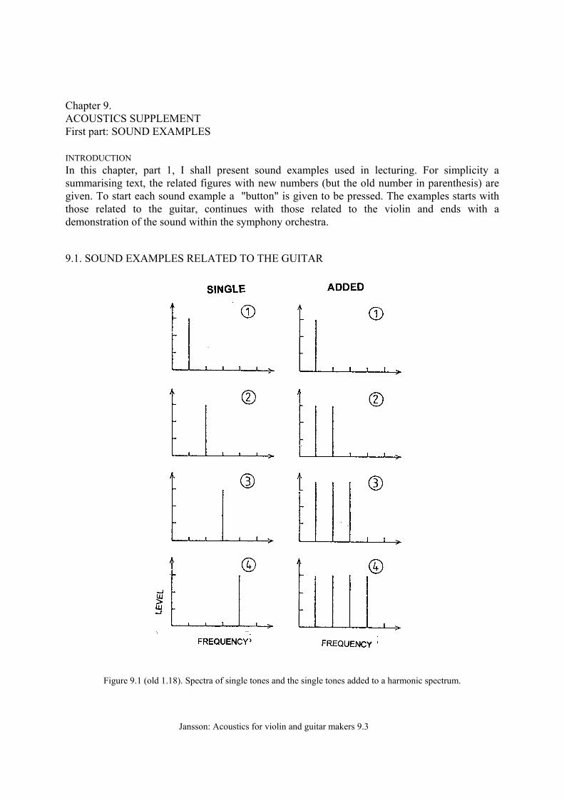
Chapter 9. ACOUSTICS SUPPLEMENT First part: SOUND EXAMPLES INTRODUCTION In this chapter, part 1, I shall present sound examples used in lecturing. For simplicity a summarising text, the related figures with new numbers (but the old number in parenthesis) are given. To start each sound example a "button" is given to be pressed. The examples starts with those related to the guitar, continues with those related to the violin and ends with a demonstration of the sound within the symphony orchestra. 9.1. SOUND EXAMPLES RELATED TO THE GUITAR

Figure 9.1 (old 1.18). Spectra of single tones and the single tones added to a harmonic spectrum.


Sound example 1. Partials and harmonic spectrum: First four single tones (partials), tone 1, 2, 3, and 4 twice. Secondly tone 1, tones 1 + 2, tones 1+2+3, and tones 1+2+3+4 (i.e. the tones (partials) separate and added in harmonic spectra, as musical tones). A simple listening exercise, sound example 1, can be prepared as shown in Fig. 9.1. The single partials 1 through 4 give tones with little character and without roughness. If the partials are added a "tone" is heard, still without much character. In the spectrum of the four partials added one can still separate each of the four partials.

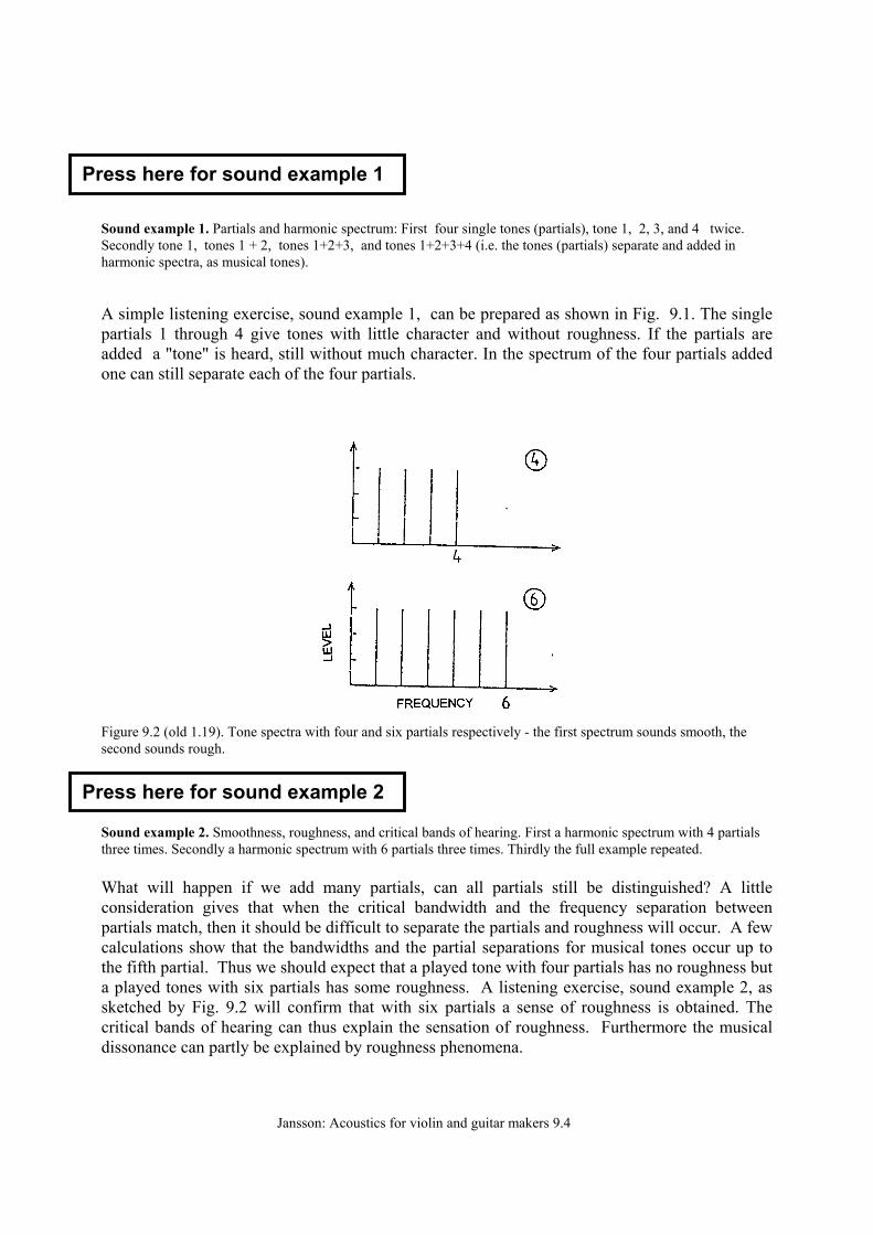
Figure 9.2 (old 1.19). Tone spectra with four and six partials respectively - the first spectrum sounds smooth, the second sounds rough. Sound example 2. Smoothness, roughness, and critical bands of hearing. First a harmonic spectrum with 4 partials three times. Secondly a harmonic spectrum with 6 partials three times. Thirdly the full example repeated. What will happen if we add many partials, can all partials still be distinguished? A little consideration gives that when the critical bandwidth and the frequency separation between partials match, then it should be difficult to separate the partials and roughness will occur. A few calculations show that the bandwidths and the partial separations for musical tones occur up to the fifth partial. Thus we should expect that a played tone with four partials has no roughness but a played tones with six partials has some roughness. A listening exercise, sound example 2, as sketched by Fig. 9.2 will confirm that with six partials a sense of roughness is obtained. The critical bands of hearing can thus explain the sensation of roughness. Furthermore the musical dissonance can partly be explained by roughness phenomena.

Press here for sound example 2



A guitar sound can be synthesised, but not by only synthesising the partial spectrum (of the string). Care must also be taken of the partials of the guitar body, the body sound. The body sound is weak but important - listen to sound example 3.

Sound example 3. Tone spectrum with body sound three times, tone spectrum only three times, body sound only three times, and tone spectrum with body sound three times.

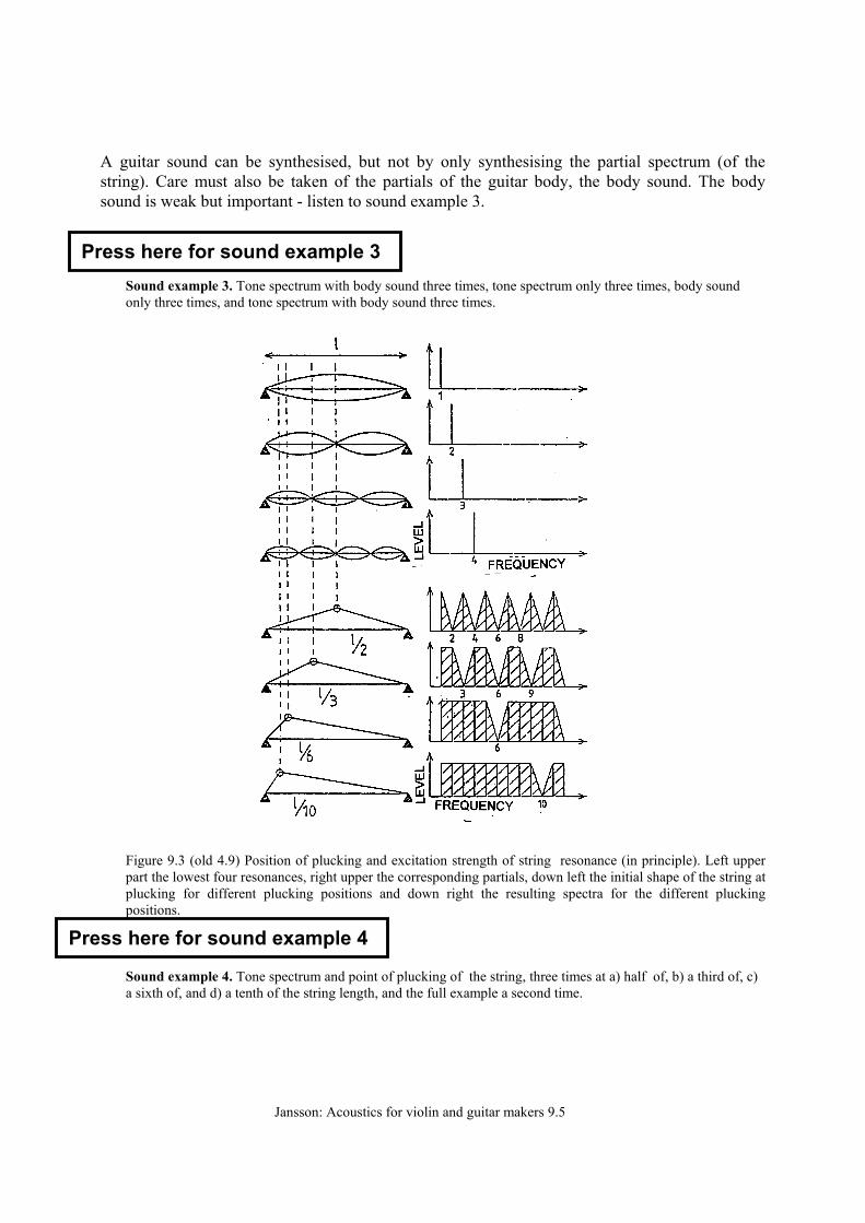
Figure 9.3 (old 4.9) Position of plucking and excitation strength of string resonance (in principle). Left upper part the lowest four resonances, right upper the corresponding partials, down left the initial shape of the string at plucking for different plucking positions and down right the resulting spectra for the different plucking positions. Sound example 4. Tone spectrum and point of plucking of the string, three times at a) half of, b) a third of, c) a sixth of, and d) a tenth of the string length, and the full example a second time.




The relation between position of plucking and the level of string partials have been sketched in fig 9.3 . When plucked in the middle, the string is initially displaced in form of a triangle with two sides alike. For a string resonance to be excited it must not be plucked at one of its nodal points. Thus we can understand that for a plucking in the middle the first partial, the fundamental is set into vibration, but not the second, the third is set into vibration, but not the fourth etc.. Thereby we obtain a spectrum like in the uppermost part of the lower right frame. If we choose to pluck at a third of the string length the third, the sixth etc. partials will be missing. If we pluck at a tenth of the string length the tenth, the twentieth partial, etc. will not be excited.

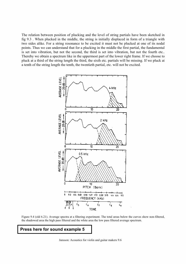
Figure 9.4 (old 6.21). Average spectra at a filtering experiment. The total areas below the curves show non-filtered, the shadowed area the high pass filtered and the white area the low pass filtered average spectrum. Press here for sound example 5


Sound example 5. The guitar and importance of different frequency bands. From Lagrima by Tarrega with the fist part broad band, the second part low-pass filtered, third part broadband, the fourth part high-pass filtered, and finally the fifth part broadband. The filter limit is set at 4 kHz the first time, 2 kHz the second time, and 500 Hz the third time.

The importance of different frequency regions (bands) can be studied with filtering and listening experiments, see Fig. 6.21. The filtering to give only components above 4 kHz demonstrate that there is only plucking sounds here. The sound filtered to give components only below 2 kHz sounds dull and hollow. With the sound filtered to below 500 Hz dull and "revelling" tones with indistinct attacks are heard. The sound filtered to above 500 Hz sounds clear but very thin.

TOO STRONG PARTIALS AT LOW FREQUENCIES GIVE DULL, HOLLOW TONES WITH INDISTINCT ATTACKS. THE HIGH PARTIALS GIVE THE TONE CLARITY, ESPECIALLY AT THE ATTACKS, BUT GIVES A THIN TONE IF THE LOWEST PARTIALS ARE TOO WEAK. THUS A BALANCE OF SEVERAL FACTORS SHOULD GIVE THE BEST INSTRUMENT.

9.2. SOUND EXAMPLES RELATED TO THE VIOLIN

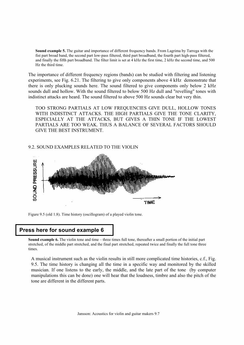
Figure 9.5 (old 1.8). Time history (oscillogram) of a played violin tone. Sound example 6. The violin tone and time – three times full tone, thereafter a small portion of the initial part stretched, of the middle part stretched, and the final part stretched, repeated twice and finally the full tone three times.

A musical instrument such as the violin results in still more complicated time histories, c.f., Fig. 9.5. The time history is changing all the time in a specific way and monitored by the skilled musician. If one listens to the early, the middle, and the late part of the tone (by computer manipulations this can be done) one will hear that the loudness, timbre and also the pitch of the tone are different in the different parts.



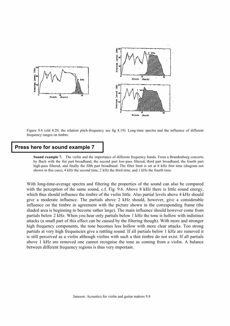
Figure 9.6 (old 8.20, the relation pitch-frequency see fig 8.19). Long-time spectra and the influence of different frequency ranges on timbre.

Sound example 7. The violin and the importance of different frequency bands. From a Brandenburg concerto by Bach with the fist part broadband, the second part low-pass filtered, third part broadband, the fourth part high-pass filtered, and finally the fifth part broadband. The filter limit is set at 8 kHz first time (diagram not shown in this case), 4 kHz the second time, 2 kHz the third time, and 1 kHz the fourth time.

With long-time-average spectra and filtering the properties of the sound can also be compared with the perception of the same sound, c.f. Fig. 9.6. Above 8 kHz there is little sound energy, which thus should influence the timbre of the violin little. Also partial levels above 4 kHz should give a moderate influence. The partials above 2 kHz should, however, give a considerable influence on the timbre in agreement with the picture shown in the corresponding frame (the shaded area is beginning to become rather large). The main influence should however come from partials below 2 kHz. When you hear only partials below 1 kHz the tone is hollow with indistinct attacks (a small part of this effect can be caused by the filtering though). With more and stronger high frequency components, the tone becomes less hollow with more clear attacks. Too strong partials at very high frequencies give a rattling sound. If all partials below 1 kHz are removed it is still perceived as a violin although violins with such a thin timbre do not exist. If all partials above 1 kHz are removed one cannot recognise the tone as coming from a violin. A balance between different frequency regions is thus very important.



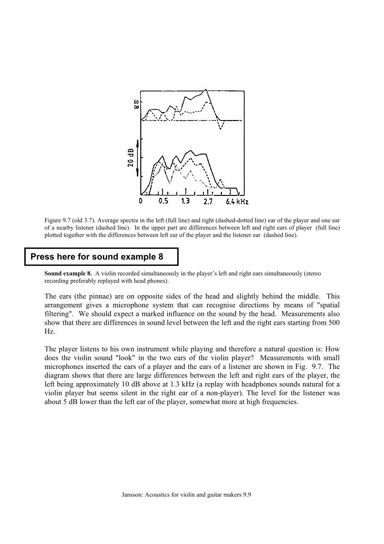
Figure 9.7 (old 3.7). Average spectra in the left (full line) and right (dashed-dotted line) ear of the player and one ear of a nearby listener (dashed line). In the upper part are differences between left and right ears of player (full line) plotted together with the differences between left ear of the player and the listener ear (dashed line). Sound example 8. A violin recorded simultaneously in the player’s left and right ears simultaneously (stereo recording preferably replayed with head phones). The ears (the pinnae) are on opposite sides of the head and slightly behind the middle. This arrangement gives a microphone system that can recognise directions by means of "spatial filtering". We should expect a marked influence on the sound by the head. Measurements also show that there are differences in sound level between the left and the right ears starting from 500 Hz. The player listens to his own instrument while playing and therefore a natural question is: How does the violin sound "look" in the two ears of the violin player? Measurements with small microphones inserted the ears of a player and the ears of a listener are shown in Fig. 9.7. The diagram shows that there are large differences between the left and right ears of the player, the left being approximately 10 dB above at 1.3 kHz (a replay with headphones sounds natural for a violin player but seems silent in the right ear of a non-player). The level for the listener was about 5 dB lower than the left ear of the player, somewhat more at high frequencies.



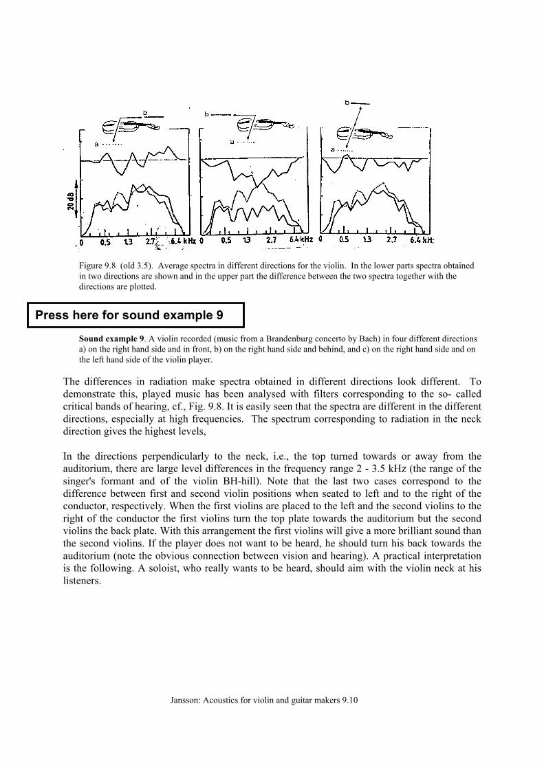
Figure 9.8 (old 3.5). Average spectra in different directions for the violin. In the lower parts spectra obtained in two directions are shown and in the upper part the difference between the two spectra together with the directions are plotted. Sound example 9. A violin recorded (music from a Brandenburg concerto by Bach) in four different directions a) on the right hand side and in front, b) on the right hand side and behind, and c) on the right hand side and on the left hand side of the violin player.

The differences in radiation make spectra obtained in different directions look different. To demonstrate this, played music has been analysed with filters corresponding to the so- called critical bands of hearing, cf., Fig. 9.8. It is easily seen that the spectra are different in the different directions, especially at high frequencies. The spectrum corresponding to radiation in the neck direction gives the highest levels, In the directions perpendicularly to the neck, i.e., the top turned towards or away from the auditorium, there are large level differences in the frequency range 2 - 3.5 kHz (the range of the singer's formant and of the violin BH-hill). Note that the last two cases correspond to the difference between first and second violin positions when seated to left and to the right of the conductor, respectively. When the first violins are placed to the left and the second violins to the right of the conductor the first violins turn the top plate towards the auditorium but the second violins the back plate. With this arrangement the first violins will give a more brilliant sound than the second violins. If the player does not want to be heard, he should turn his back towards the auditorium (note the obvious connection between vision and hearing). A practical interpretation is the following. A soloist, who really wants to be heard, should aim with the violin neck at his listeners.



9.3. SOUND EXAMPLES RELATED TO THE ORCHESTRA

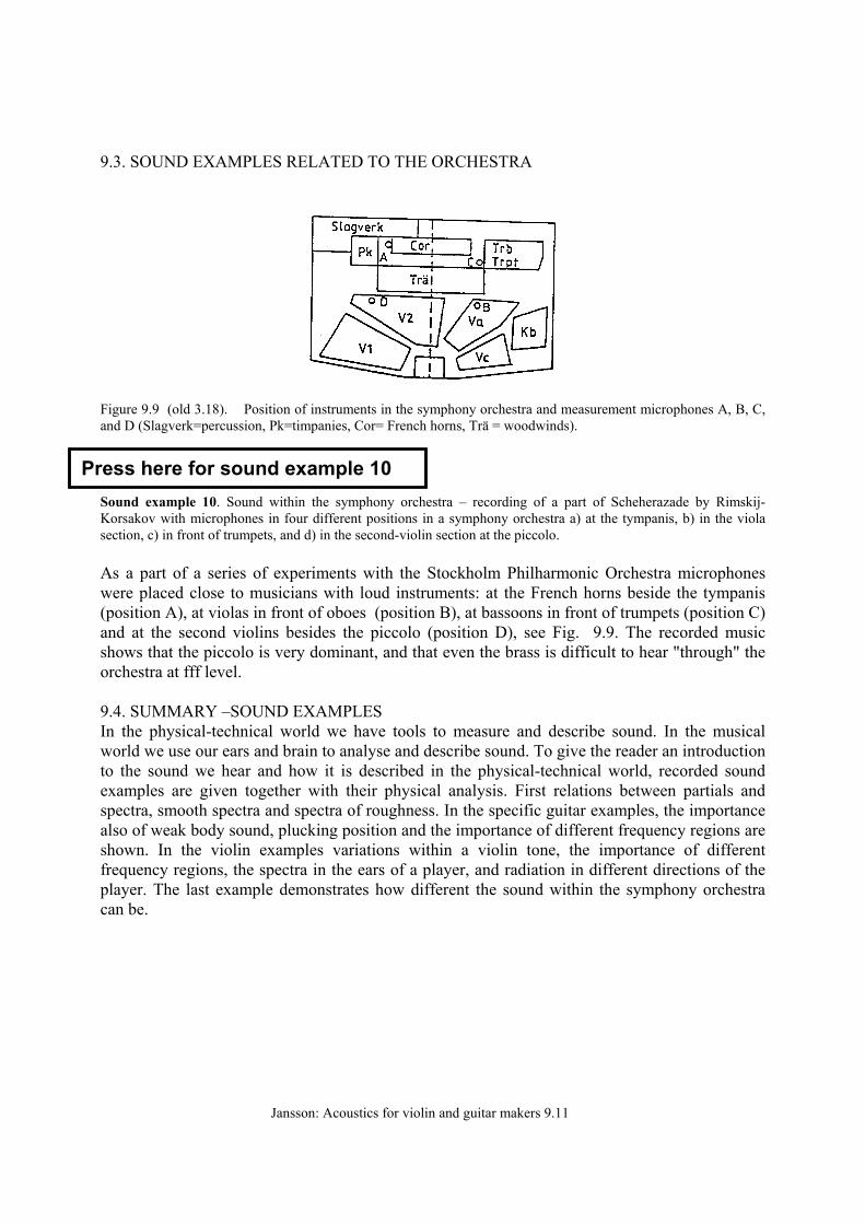
Figure 9.9 (old 3.18). Position of instruments in the symphony orchestra and measurement microphones A, B, C, and D (Slagverk=percussion, Pk=timpanies, Cor= French horns, Trä = woodwinds). Sound example 10. Sound within the symphony orchestra – recording of a part of Scheherazade by Rimskij-Korsakov with microphones in four different positions in a symphony orchestra a) at the tympanis, b) in the viola section, c) in front of trumpets, and d) in the second-violin section at the piccolo. As a part of a series of experiments with the Stockholm Philharmonic Orchestra microphones were placed close to musicians with loud instruments: at the French horns beside the tympanis (position A), at violas in front of oboes (position B), at bassoons in front of trumpets (position C) and at the second violins besides the piccolo (position D), see Fig. 9.9. The recorded music shows that the piccolo is very dominant, and that even the brass is difficult to hear "through" the orchestra at fff level. 9.4. SUMMARY –SOUND EXAMPLES In the physical-technical world we have tools to measure and describe sound. In the musical world we use our ears and brain to analyse and describe sound. To give the reader an introduction to the sound we hear and how it is described in the physical-technical world, recorded sound examples are given together with their physical analysis. First relations between partials and spectra, smooth spectra and spectra of roughness. In the specific guitar examples, the importance also of weak body sound, plucking position and the importance of different frequency regions are shown. In the violin examples variations within a violin tone, the importance of different frequency regions, the spectra in the ears of a player, and radiation in different directions of the player. The last example demonstrates how different the sound within the symphony orchestra can be.



CHAPTER 9. Second part: SIMPLE EXPERIMENTAL MATERIAL

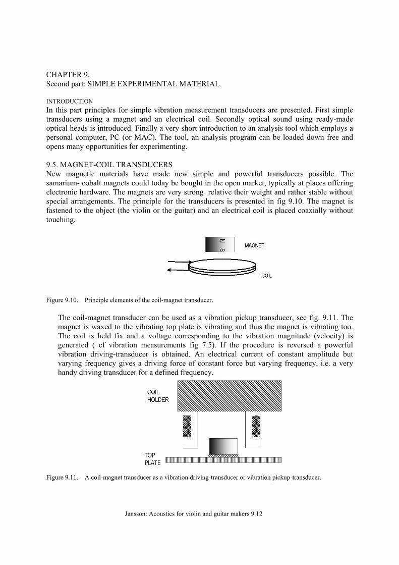
INTRODUCTION In this part principles for simple vibration measurement transducers are presented. First simple transducers using a magnet and an electrical coil. Secondly optical sound using ready-made optical heads is introduced. Finally a very short introduction to an analysis tool which employs a personal computer, PC (or MAC). The tool, an analysis program can be loaded down free and opens many opportunities for experimenting. 9.5. MAGNET-COIL TRANSDUCERS New magnetic materials have made new simple and powerful transducers possible. The samarium- cobalt magnets could today be bought in the open market, typically at places offering electronic hardware. The magnets are very strong relative their weight and rather stable without special arrangements. The principle for the transducers is presented in fig 9.10. The magnet is fastened to the object (the violin or the guitar) and an electrical coil is placed coaxially without touching.

Figure 9.10. Principle elements of the coil-magnet transducer. The coil-magnet transducer can be used as a vibration pickup transducer, see fig. 9.11. The magnet is waxed to the vibrating top plate is vibrating and thus the magnet is vibrating too. The coil is held fix and a voltage corresponding to the vibration magnitude (velocity) is generated ( cf vibration measurements fig 7.5). If the procedure is reversed a powerful vibration driving-transducer is obtained. An electrical current of constant amplitude but varying frequency gives a driving force of constant force but varying frequency, i.e. a very handy driving transducer for a defined frequency.

Figure 9.11. A coil-magnet transducer as a vibration driving-transducer or vibration pickup-transducer.


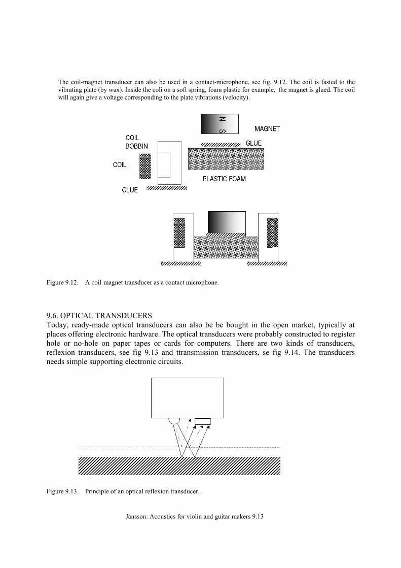
The coil-magnet transducer can also be used in a contact-microphone, see fig. 9.12. The coil is fasted to the vibrating plate (by wax). Inside the coli on a soft spring, foam plastic for example, the magnet is glued. The coil will again give a voltage corresponding to the plate vibrations (velocity).

Figure 9.12. A coil-magnet transducer as a contact microphone.

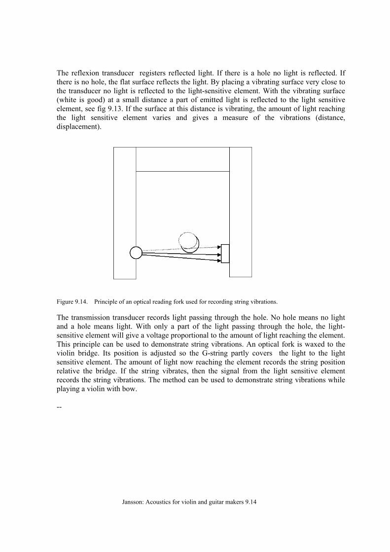
9.6. OPTICAL TRANSDUCERS Today, ready-made optical transducers can also be be bought in the open market, typically at places offering electronic hardware. The optical transducers were probably constructed to register hole or no-hole on paper tapes or cards for computers. There are two kinds of transducers, reflexion transducers, see fig 9.13 and ttransmission transducers, se fig 9.14. The transducers needs simple supporting electronic circuits.

Figure 9.13. Principle of an optical reflexion transducer.


The reflexion transducer registers reflected light. If there is a hole no light is reflected. If there is no hole, the flat surface reflects the light. By placing a vibrating surface very close to the transducer no light is reflected to the light-sensitive element. With the vibrating surface (white is good) at a small distance a part of emitted light is reflected to the light sensitive element, see fig 9.13. If the surface at this distance is vibrating, the amount of light reaching the light sensitive element varies and gives a measure of the vibrations (distance, displacement).

Figure 9.14. Principle of an optical reading fork used for recording string vibrations. The transmission transducer records light passing through the hole. No hole means no light and a hole means light. With only a part of the light passing through the hole, the light-sensitive element will give a voltage proportional to the amount of light reaching the element. This principle can be used to demonstrate string vibrations. An optical fork is waxed to the violin bridge. Its position is adjusted so the G-string partly covers the light to the light sensitive element. The amount of light now reaching the element records the string position relative the bridge. If the string vibrates, then the signal from the light sensitive element records the string vibrations. The method can be used to demonstrate string vibrations while playing a violin with bow. --


9.7. COMPUTER ANALYSIS (PC or Macintosh)

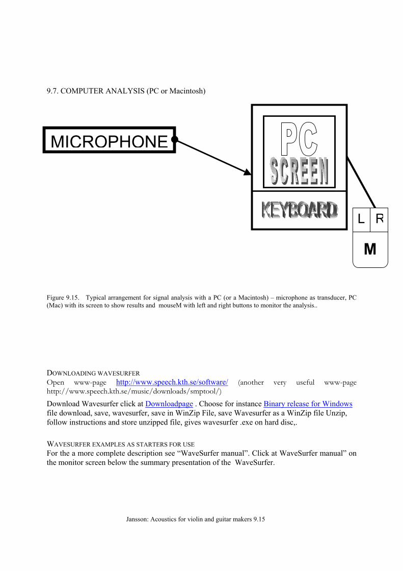
Figure 9.15. Typical arrangement for signal analysis with a PC (or a Macintosh) – microphone as transducer, PC (Mac) with its screen to show results and mouseM with left and right buttons to monitor the analysis.. DOWNLOADING WAVESURFER Open www-page http://www.speech.kth.se/software/ (another very useful www-page http://www.speech.kth.se/music/downloads/smptool/) Download Wavesurfer click at Downloadpage . Choose for instance Binary release for Windows file download, save, wavesurfer, save in WinZip File, save Wavesurfer as a WinZip file Unzip, follow instructions and store unzipped file, gives wavesurfer .exe on hard disc,. WAVESURFER EXAMPLES AS STARTERS FOR USE For the a more complete description see “WaveSurfer manual”. Click at WaveSurfer manual” on the monitor screen below the summary presentation of the WaveSurfer.

MICROPHONE

M

L R


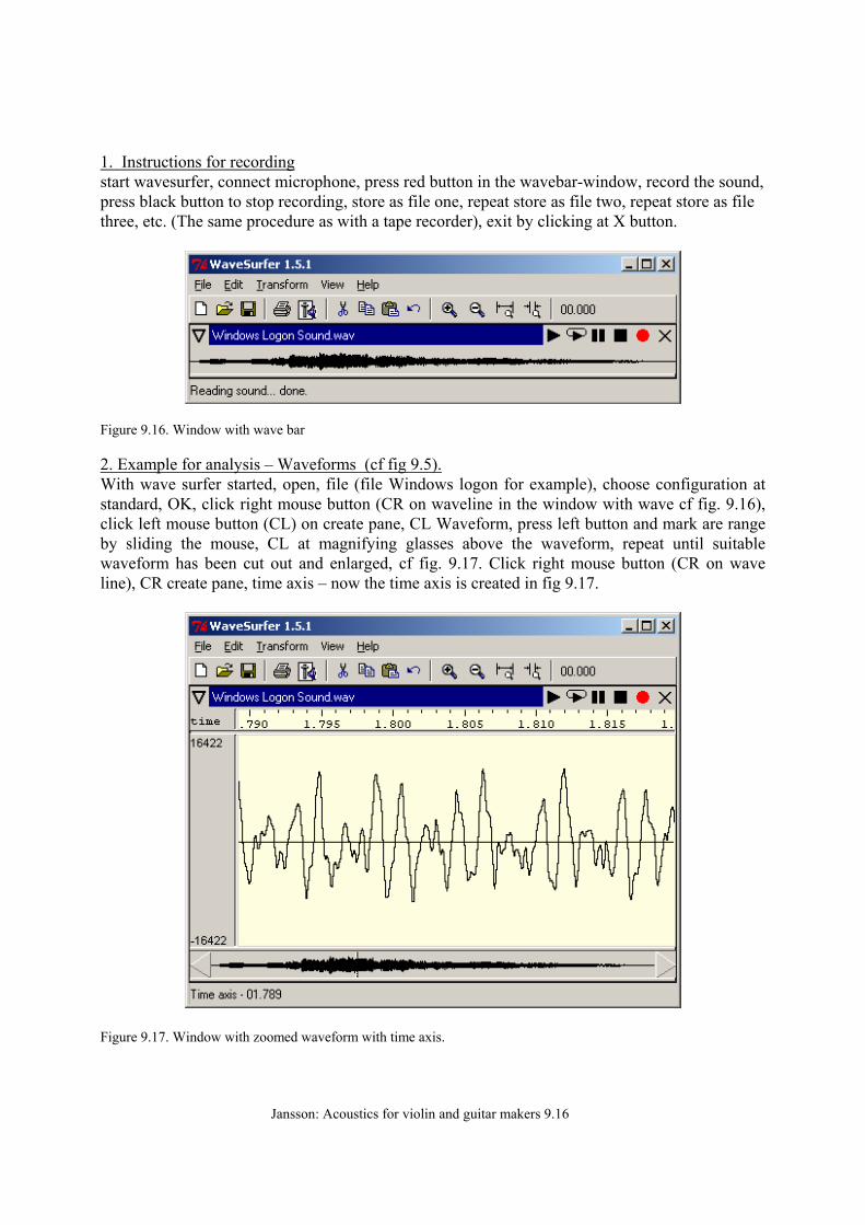
1. Instructions for recording start wavesurfer, connect microphone, press red button in the wavebar-window, record the sound, press black button to stop recording, store as file one, repeat store as file two, repeat store as file three, etc. (The same procedure as with a tape recorder), exit by clicking at X button.

Figure 9.16. Window with wave bar 2. Example for analysis – Waveforms (cf fig 9.5). With wave surfer started, open, file (file Windows logon for example), choose configuration at standard, OK, click right mouse button (CR on waveline in the window with wave cf fig. 9.16), click left mouse button (CL) on create pane, CL Waveform, press left button and mark are range by sliding the mouse, CL at magnifying glasses above the waveform, repeat until suitable waveform has been cut out and enlarged, cf fig. 9.17. Click right mouse button (CR on wave line), CR create pane, time axis – now the time axis is created in fig 9.17.

Figure 9.17. Window with zoomed waveform with time axis.


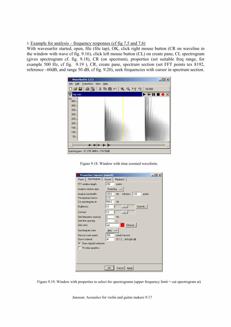
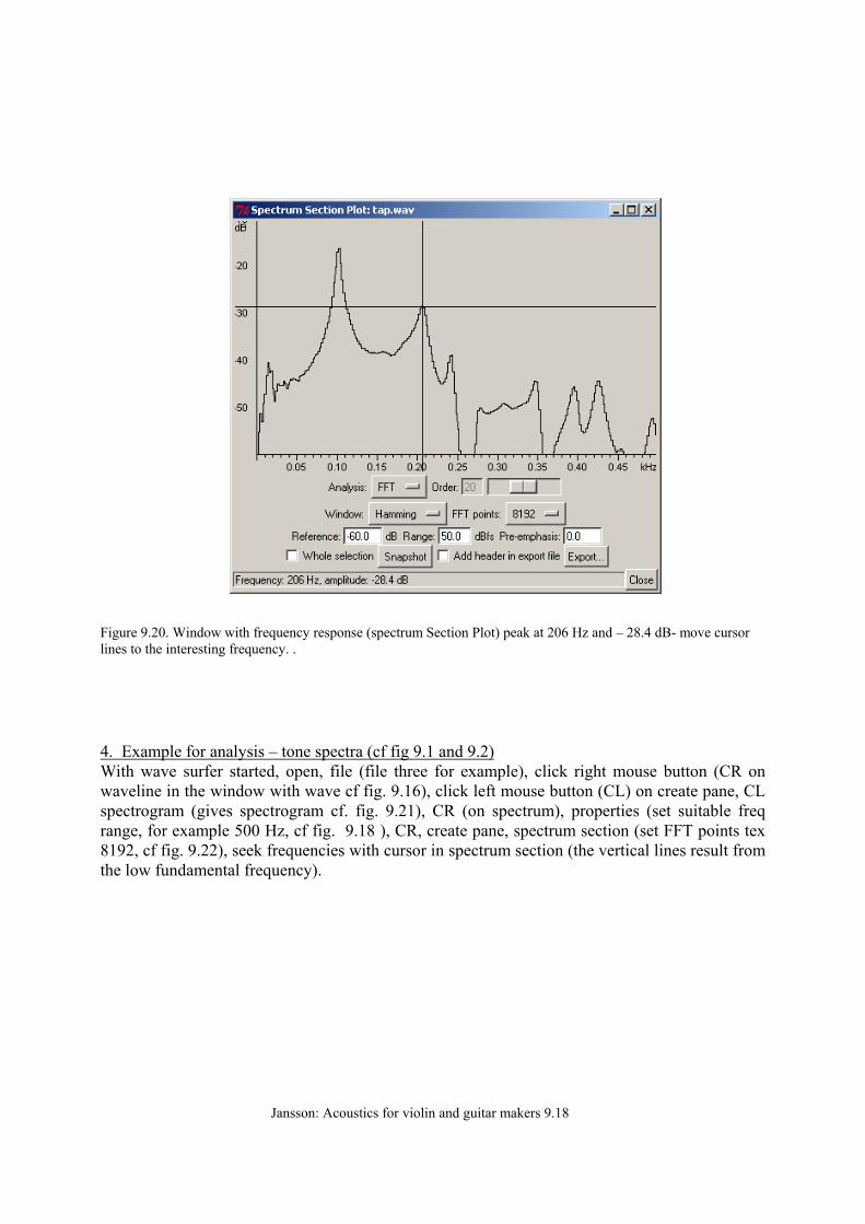
3. Example for analysis – frequency responses (cf fig 7.5 and 7.6) With wavesurfer started, open, file (file tap), OK, click right mouse button (CR on waveline in the window with wave cf fig. 9.16), click left mouse button (CL) on create pane, CL spectrogram (gives spectrogram cf. fig. 9.18), CR (on spectrum), properties (set suitable freq range, for example 500 Hz, cf fig. 9.19 ), CR, create pane, spectrum section (set FFT points tex 8192, reference –60dB, and range 50 dB, cf fig. 9.20), seek frequencies with cursor in spectrum section.

Figure 9.18. Window with time-zoomed waveform.

Figure 9.19. Window with properties to select for spectrograms (upper frequency limit = cut spectrogram at)


Figure 9.20. Window with frequency response (spectrum Section Plot) peak at 206 Hz and – 28.4 dB- move cursor lines to the interesting frequency. .

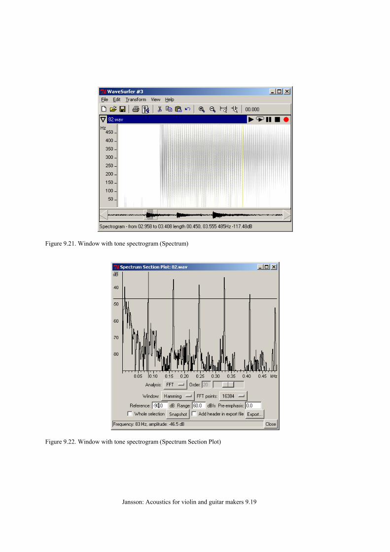
4. Example for analysis – tone spectra (cf fig 9.1 and 9.2) With wave surfer started, open, file (file three for example), click right mouse button (CR on waveline in the window with wave cf fig. 9.16), click left mouse button (CL) on create pane, CL spectrogram (gives spectrogram cf. fig. 9.21), CR (on spectrum), properties (set suitable freq range, for example 500 Hz, cf fig. 9.18 ), CR, create pane, spectrum section (set FFT points tex 8192, cf fig. 9.22), seek frequencies with cursor in spectrum section (the vertical lines result from the low fundamental frequency).


Figure 9.21. Window with tone spectrogram (Spectrum)

Figure 9.22. Window with tone spectrogram (Spectrum Section Plot)


9.8. SUMMARY – SIMPLE EXPERIMENTAL MATERIAL Two simple and powerful vibration measurement transducers have been presented. First the coil-magnet transducer, secondly the optical transducer. The coil-magnet transducers need some coil-windings but are therafter ready to use. Parts for the optical transducers can be bought ready – only some supporting eectronics must be built. The computer program Wavesurfer can loaded down free and can be used on most personal computer systems. The experimenter can develop his own analysis.

Documents

ACOUSTICS FOR VIOLIN AND GUITAR MAKERS · VIOLIN AND GUITAR MAKERS Erik Jansson ... Position of plucking and excitation strength of string ... on the right hand side and on the left