ACROPORA PALMATA - getd.libs.uga.edu

UNDERSTANDING AND PREDICTING CORAL DISEASE ACROSS SCALES: WHITE

POX DISEASE AND THE CRITICALLY-ENDANGERED ELKHORN CORAL, ACROPORA

PALMATA

by

ASHTON PHILLIPS GRIFFIN

(Under the Direction of Andrew W. Park and James W. Porter)

ABSTRACT

Outbreaks of infectious disease events in the marine environment often occur with little warning

and can have severe consequences for their host populations. Infectious disease events in corals

have increased over the last decade, coinciding with the continuing decline of the reef

environment on a global scale. Understanding and predicting future disease events will be a

critical step towards developing a response strategy. This dissertation provides a multi-scale

approach towards understanding white pox disease, a disease that affects the import reef-

building, yet critically endangered, coral, Acropora palmata. I first explore the diversity found

within the surface mucus layer of A. palmata. I accomplish this through by measuring the alpha

diversity from mucus samples collected from healthy, bleached, and diseased colonies. Species

richness was greatest in samples from diseased corals. Seasonality was an important driver in

distinguishing microbial communities. I also developed a statistical framework to identify factors

influencing local disease transmission. Using this framework, I fit models to data collected

during an outbreak of white pox disease and determined spatial diffusion provided the best fit.

Using simulations, I then evaluated how censored surveillance data influenced model

performance. Last, using biological and environmental data obtained over a 20-yr time period, I

constructed a machine learning model that predicted disease occurrence in individual A. palamta

colonies. This approach used a large set of environmental variables to predict disease presence or

absence. Collectively, these results suggest that microbial communities are different between

healthy and diseased, proximity to nearby infected is important for disease transmission, and

disease event can be predicted by colony size, dissolved saturated oxygen, wind speed, and

organic carbon.

INDEX WORDS: White pox disease; Acropora palmata; microbiome; pathogen

transmission; disease prediction



PALMATA

by

ASHTON GRIFFIN

BS, University of Georgia, 2010

A Dissertation Submitted to the Graduate Faculty of The University of Georgia in Partial

Fulfillment of the Requirements for the Degree

DOCTOR OF PHILOSOPHY

ATHENS, GEORGIA

2018

© 2018

Ashton Phillips Griffin

All Rights Reserved



PALMATA

by

ASHTON PHILLIPS GRIFFIN

Major Professors: Andrew W. Park

James Porter

Committee: Craig Osenberg

Deepak Mishra

Marguerite Madden

Electronic Version Approved:

Suzanne Barbour

Dean of the Graduate School

The University of Georgia

May 2018

iv

DEDICATION

For Haylee.

v

ACKNOWLEDGEMENTS

Could not have been done without my committee, Haylee, and numerous mentors across

the years.

vi

TABLE OF CONTENTS

Page

ACKNOWLEDGEMENTS .............................................................................................................v

LIST OF TABLES ........................................................................................................................ vii

LIST OF FIGURES ....................................................................................................................... ix

CHAPTER

1 INTRODUCITON AND LITERATURE REVIEW .....................................................1

2 CHARACTERIZING MICROBIAL COMMUNITIES WITHIN SURFACE MUCUS

FROM HEALTHY, BLEACHED, AND DISEASED ELKHORN CORAL .................7

3 INVESTIGATING THE IMPORTANCE OF LOCAL SPATIAL STRUCTURE

AND COLONY SIZE IN THE TRANSMISSION OF WHITE POX .......................42

4 BIOTIC AND ABIOTIC DRIVERS OF WHITE POX DISEASE IN ELKHORN

CORAL OVER 20 YEARS IN THE FLORIDA KEYS .............................................81

5 CONCLUSIONS........................................................................................................132

REFERENCES ............................................................................................................................138

vii

LIST OF TABLES

Page

Table 2.1: Sample summary and diversity for sample type and season ........................................27

Table 2.2: Output from linear mixed effect model for species richness (Chao1) .........................28

Table 2.3: Output from linear mixed effect model for microbial community (Shannon-Wiener) 29

Table 2.4: Output from linear mixed effect model for species evenness (Pielou’s J) ...................30

Table 2.5: Permanova analysis on PCoA using weighted unifrac with interaction between sample

type and season ..................................................................................................................31

Table 3.1: Description and forms for competing models of disease transmission ........................66

Table 3.2: Model performance from empirical fit .........................................................................68

Table 3.3: Estimated parameters for each model from maximum likelihood estiamtion ..............69

Table 3.4: Model selection from data degradation simulation .....................................................70

Table 4.1: Summary of surveillance for expanded study ............................................................103

Table 4.2: Summary of predictor variables..................................................................................104

Table 4.3: Matching sites between surveillance and SERC ........................................................106

Table 4.4: Boosted regression tree hyperparameters ...................................................................107

Table 4.5: Geogam model index ..................................................................................................108

Table 4.6: Full training output .....................................................................................................109

Table 4.7: Full testing output .......................................................................................................110

Table 4.8: Full interaction values .................................................................................................111

Table 4.9: Simplified training output ...........................................................................................112

viii

Table 4.10: Simplified testing output...........................................................................................113

Table 4.11: Simplified interactions ..............................................................................................114

Table 4.12: Relative influence from the full model .....................................................................115

ix

LIST OF FIGURES

Page

Figure 2.1: Distribution of sequencing depth ................................................................................32

Figure 2.2: Species richness with Chao1 by sample type .............................................................33

Figure 2.3: Species richness with Chao1 by season ......................................................................34

Figure 2.4: Shannon-Wiener index for microbial communities by sample type ...........................35

Figure 2.5: Shannon-Wiener index for microbial communities by season ....................................36

Figure 2.6: Species evenness with Pielou’s J by sample type .......................................................37

Figure 2.7: Species evenness with Pielou’s J by season ................................................................38

Figure 2.8: PCoA plots by season and sample type with ellipsoids ..............................................39

Figure 2.9: Relative abundances of taxonomic families by sample type .......................................40

Figure 2.10: Relative abundances of taxonomic families by season .............................................41

Figure 3.1: Diagram outlining the degradation scenarios used in simulation................................71

Figure 3.2: Tracking individual health status through time ...........................................................73

Figure 3.3: Observed incidence of disease ....................................................................................74

Figure 3.4: Observed disease prevalence .......................................................................................75

Figure 3.5: Relationship between size and disease status from first month of surveillance ..........76

Figure 3.6: Distribution of sizes between infected and uninfected observations ..........................77

Figure 3.7: Results from goodness of fit estimation ......................................................................78

Figure 3.8: Results from simulating white pox disease epidemic .................................................79

Figure 4.1: Map of study area ......................................................................................................118

x

Figure 4.2: Receiver operating curve for the full model ..............................................................119

Figure 4.3: Relative influence for predictor variables form full model .......................................120

Figure 4.4: Partial dependency plots of six most influential variable from full model ...............121

Figure 4.5: Interaction plot for colony size and sea surface temperature from full model ..........122

Figure 4.6: Interaction plot for colony size and dissolved saturated oxygen from full model ...123

Figure 4.7: Interaction plot for colony size and total organic carbon from the full model ..........124

Figure 4.8: Interaction plot for colony size and wind speed from the full model .......................125

Figure 4.9: Receiver operating curve from the simplified model ................................................126

Figure 4.10: Relative influence for predictor variables from the simplified model ....................127

Figure 4.11: Paratial dependency plot from the four variables from the simplified model .........127

Figure 4.12: Interaction plot for colony size and wind speed from the simplified model ..........129

Figure 4.13: Interaction plot between colony size and dissolved saturated oxygen from the

simplified model ..............................................................................................................130

Figure 4.14: AUC values from various geoGAM models ...........................................................131

Figure 4.15: AResults from cross validation of water temperature .............................................132

CHAPTER 1

INTRODUCTION AND LITERATURE REVIEW

Outbreaks of infectious diseases in the marine environment are typically sudden and can have

severe consequences for affected populations. In 1983 a massive die off of the sea urchin

Diadema antillarum was observed throughout the Caribbean 1. A high rate of spread that

traveled predominantly along prevailing currents provided evidence that the underlying driver of

the mortality event was an emerging waterborne pathogen 2. From 2013 to 2015, approximately

20 different species of sea stars (asteroids) washed ashore along the west coast of North America

due to an outbreak of sea star wasting disease 3,4. While outbreaks of sea star wasting disease

have been observed in previous decades, the 2013 – 2015 outbreak was exceptional with respect

to spatial scale and number of populations affected 4. In 1994, a previously unidentified coral

disease affected an important reef building coral, Acropora palmata 5. Subsequently, A. palmata

(a scleractinian coral also known as elkhorn coral) was designated as a threatened species under

the US Endangered Species Act in 2006, in part due to pathogen pressure but also because of

storm damage and ocean acidification6–8. Despite the increased attention given to marine

diseases in recent years, our understanding of mechanisms for transmission, environmental

drivers, and microbial interactions is still quite limited 9.

Over time, quantitative methods have been developed to aid our understanding of disease

ecology10. Classical models of infectious disease dynamics have allowed researchers to evaluate

the rate at which susceptible individuals become infected, the average number of new infections

one infected individual will generate, and the number of immune individuals needed to eradicate

1

pathogens 11. Much of the quantitative methodology in this field was initially developed for

human diseases11. As appropriate data became available, these quantitative methods have been

adapted to wildlife diseases12. In an example relevant to coral disease, gravity models (Chapter

3) were initially developed to help understand the spread of measles at the landscape level and

then later adapted and applied to understand the spread of a fungal pathogen in North American

bat populations 13,14. In plant diseases, models have been well developed to account for

spatiotemporal dynamics, host resistance, pathogen inoculum intensity, and environmental

factors 15–18. By comparison, theoretical modeling of marine diseases remain underdeveloped 9,19.

In recent decades, researchers have documented the ongoing coral reef crisis across the

globe as the ecosystem has continued to decline. Percent live cover of corals in the Caribbean

declined by 80% from 1977 to 2003 7. On the Great Barrier Reef a 50% reduction in live cover

occurred from 1985 to 2012 20. Coral cover in the Indo-Pacific declined by 50% from the 1980s

to 2003 21. Climate change has played an important role as a driver of events associated with the

global decline in coral cover 22–25. Declines in coral cover have been associated with the

occurrence of tropical cyclones 7,20,21. Coral bleaching, a condition where the coral animal loses

its symbiotic algae, is typically caused by thermal stress 26–28. Massive coral bleaching events, in

which entire reef tracts are bleached simultaneously are occurring more frequently due to climate

change 29. Coral diseases have also contributed to the loss of coral cover in recent decades 30–33.

Researchers have begun to establish associations between disease occurrence and environmental

conditions 34,35.

The first reported case of any coral disease was a description of growth anomalies that

were observed on a Hawaiian reef 36. Currently, there are 18 well defined diseases affecting

2

scleractinian coral of which 12 are found in Caribbean coral 32,37,38. From the 18 described

diseases, 9 have established pathogens 39. Recently, researchers proposed the ‘moving target’

hypothesis, which proposes that multiple pathogens (operating either jointly or independently)

can cause the symptoms of a disease 39. Evidence for the moving target hypothesis has been

documented for white pox disease 39. First observed in 1994, white pox disease (also known as

white-patch, or patchy necrosis) affects the Caribbean reef building coral Acropora palmata

5,32,40,41, with studies during subsequent outbreaks of white pox over nearly a decade reporting an

average reduction of 85% in live coral cover 32. Symptoms of white pox are described as

irregularly shaped white patches that appear on the surface of the colony 41,42. Edges between

live tissue and diseased tissue are distinct, with an loss rate of between 2.1 and 7.5 cm2 per day

on average respectively 32,41. The first causative agent to be identified for white pox was the fecal

enterobacterium Serratia marcescens 32. In a recent study, researchers failed to detect the

presence of S. marcescens in any white pox samples 43. In a follow-up study, researchers were

able to detect the presence of S. marcescens in some samples of white pox but not all 39.

However, evidence from Sutherland et al. (2016)39 suggests that historical cases of white pox

(which were positive for S. marcescens) had higher measures of disease severity and mortality

compared to contemporary cases 39. The inability to recover S. marcescens from recent samples

of white pox is consistent with the moving target hypothesis, suggesting that changes in host

genotype and environmental conditions can give rise to shifts in the etiology of disease 39.

Understanding the mechanisms behind the moving target hypothesis requires a deeper

understanding of coral disease biology, prefaced by increasing our understanding of the effect of

coral microbial communities, factors influencing pathogen transmission, and identification of

biotic and abiotic drivers of disease occurrence.

3

Of the microhabitats found in coral, the surface mucus layer is believed to play an

important role in the resistance to, and recovery from, coral disease 44–48. Beneficial microbes

found within the mucus surface layer can provide resistance by secreting antibiotic compounds

into surrounding mucus as observed in microbial samples taken from A. palmata 49, which inhibit

the growth of S. marcescens 50. Quorum sensing and microbial predation are two other possible

mechanisms that microbial communities can utilize to provide resistance to disease 51,52.

However, like many aspects of the coral microbial community, research is still in the early stages

and more work is needed to establish the ubiquity of these mechanisms 48. Our understanding of

coral microbial communities with respect to disease has been advancing rapidly, and new lines

of research identify a need to study how microbial communities vary across multiple scales 47. A

critical step towards this goal would be to better understand how diseases, and potentially

beneficial microbes, develop within and spread between coral colonies.

Despite research on coral disease dating back to the 1970s 37, we have a limited

understanding of the factors that contribute to the transmission of pathogens that cause coral

diseases. Perhaps part of the reason for limited knowledge of transmission lies with our poor

understanding of causative agents 39. However, lack of robust surveillance data due to costs and

incomplete understanding of environmental drivers for each disease contribute to this knowledge

gap 53. Initial efforts have either examined spatial patterns of diseased and non-diseased

individuals 54–56 or adapted a metapopulation model for transmission 57. These approaches have

indicated that local spatial structure is important for the spread of disease within reefs, but few

have tested competing hypotheses of spread 56. Competing multiple hypotheses of disease spread

requires a framework that can be flexible to account for different potential spread mechanisms

and for which typical levels of surveillance data are sufficient to evaluate their differential

4

performance, allowing the framework to identify one or more supported hypotheses. In turn,

mechanistic and statistical models describing transmission and outbreak risk in terms of abiotic

and biotic factors may inform the collection of appropriate surveillance data, for example, by

identifying at-risk colonies or reefs before an outbreak event.

In recent years, coral biologists have begun leveraging available surveillance and

environmental data to investigate the relationships between environmental factors (separate from

host, pathogen and microbiome organisms) and disease occurrence, as well as their potential

interaction with biological factors such as colony live tissue cover. Environmental factors may

promote disease occurrence either directly, by inducing dysbiosis, a strong imbalance in

microbial communities 58,59, or indirectly by affecting host or pathogen health 57. For many

systems, parameters derived from remote measurement of sea surface temperature have

demonstrated an association between outbreaks of disease and elevated temperature 34,35,55,60,61.

Additional environmental factors such as nutrient concentration have been observed to increase

the severity of disease events 62,63. Biological factors such as host size and density have also been

shown to contribute to outbreaks of disease across a range of coral species 34,54,64,65.

Understanding the relationships between climate, water quality, and biotic disease predictors and

how they contribute to disease risk will inform researchers and managers when and where

disease events are likely to occur. Predictions of such disease events would help target

logistically-constrained disease surveillance, implement management techniques, and inform

policy development to reduce the risk of future outbreaks 4. However, before predictive models

can be constructed a sufficient level of banked surveillance work is needed to help train and test

statistical models.

5

The objective of this dissertation is to examine the spatio-temporal dynamics of white

pox disease in A. palmata across multiple scales, to better understand the importance of inter-

individual colony variation in host microbial community, to establish factors influencing

pathogen transmission between colonies within a site, and to determine drivers of disease

occurrence at broader spatial scales encompassing multiple reefs. In Chapter 2, I examine the

microbial diversity taken from surface mucus samples of healthy and unhealthy A. palmata

colonies at three-time points within a year. In Chapter 3, I present and implement a statistical

framework that allows for competing hypotheses regarding transmission between colonies using

surveillance data collected from an outbreak of white pox disease at one site. These competing

hypotheses include effects of infected and uninfected colony size, inter-colony distance and

mechanistic interactions between them. Lastly, Chapter 4 leverages two decades of white pox

disease surveillance data in the Florida Keys to assess how the combination of remotely sensed

environmental data, locally collected water quality data, and colony-level data can be used to

develop a predictive model that accurately determines locations and time points at which coral

are at risk of disease outbreaks. The outcome of this dissertation is a contribution to our

understanding of disease in a critically endangered reef building coral. More broadly, these

findings and methodologies will help elucidate the nature of diseases in the marine environment

and develop statistical approaches to may assist with the investigation of future outbreaks.

6

CHAPTER 2

CHARACTERIZING MICROBIAL COMMUNITIES WITHIN SURFACE MUCUS FROM

HEALTHY, BLEACHED, AND DISEASED ELKHORN CORAL1

1 Griffin AP, Kaul RB, Kemp DW, Wares JP, Porter JW, Park AW. To be submitted to Frontiers in

Marine Science.

7

Abstract

The coral surface mucus layer is a main component in the coral holobiont and studying the

associated microbial communities is anticipated to provide a better understanding of the

occurrence, progression of, and response to disease events. We studied the microbial diversity of

surface mucus samples that were collected from healthy, bleached, and white pox diseased

Acropora palmata colonies across three seasons within a year. Microbial species richness was

greater in samples that were collected from lesions of white pox relative to samples from healthy

corals. We also found that microbial communities varied seasonally, and that this variation was

greater than that observed among corals that were diseased, bleached, or healthy. These findings

suggest that white pox disease can disrupt the microbial community found in the surface mucus

of healthy A. palamta colonies. Furthermore, results also suggest that seasonality is an important

component of the dynamics of microbial diversity of coral.

Introduction

The study of biological diversity seeks to understand the assemblage of species within a given

community. Biodiversity is typically assessed with two general concepts: species richness, which

addresses the number of unique species within a community; and species evenness, which

accounts for the relative abundance of each species in the community. Although specific metrics

of biodiversity are still debated 66, a growing body of literature seeks to understand the many

ways in which biodiversity affects pathogen transmission. For example, the dilution effect

hypothesis posits that disease risk is reduced in communities that have relatively high abundance

of host species that do not contribute greatly to parasite fitness 67. In recent years, due to

advancement of genomic sequencing techniques, microbial ecologists have begun exploring

connections between microbial communities, that exist in or on host individuals, and disease.

8

Dysbiosis, an imbalance in a microbial community, has been associated with inflammatory

bowel disease, Crohn’s disease, and caries (mouth cavities) in humans 68–70. In amphibians, skin

pathogens can lead to disruptions in the skin mucosome microbial communities of affected hosts

71. Furthermore, experimental shifts in temperature lead to functional changes in mucosal

microbial communities resulting in increased prevalence of disease 72. While less researched,

microbial communities in corals are thought to play a significant role in maintaining colony

health 47,73.

The coral holobiont is defined as the cooperative interactions between the colony,

zooxanthellae, and microbial communities that contribute to colony fitness 74. Associated

microbial communities can contribute to coral health in a variety of ways. A large proportion of

a coral’s carbon requirement is provided through a symbiotic relationship with the coral’s

zooxanthellae 75. However, other essential nutrients are typically provided by the microbial

community. For example, cyanobacteria and diazotrophs are thought to provide a significant

amount of nitrogen to the coral via nitrogen fixation 76,77. An experimental study provided

evidence suggesting microbial communities play an important role in promoting colony

resilience to environmental stressors 78. Certain surface mucus layer microbes are believed to

promote disease resistance by producing antibiotic compounds that inhibit the growth of known

coral pathogens 49,79. In recent decades, researchers have sought to characterize the microbial

diversity found within coral, and to determine how environmental stress and disturbance events,

such as disease, can alter the associated microbial communities 45,47,74. The microbial community

found within the surface mucus layer of coral colonies is believed to play a vital role in the

relationship between colony and disease 80.

9

The coral’s surface mucus layer is a polysaccharide protein lipid complex that is secreted

by the coral’s epidermal mucus cells 81,82. Physical and chemical properties of surface mucus

vary between coral species 83 and chemical properties are subject to change during periods of

environmental stress 84. The observed microbial communities within the surface mucus are likely

a result of mucus properties, and microbial communities have been observed to differ under

stressful conditions. However, it is not well understood how disturbances on the colony’s surface

can influence surface mucus microbial communities or how changes in the surface mucus

microbial communities can lead to localized disturbance, including disease lesions, on the

colony’s surface tissue.

Studying the microbial communities found in surface mucus may provide insights into

the nature of coral disease occurrence and colony resilience 39. In some cases previous research

has failed to detect consistent causes of disease, and for many coral diseases the causative agent

for disease is still debated 76,85. The difficulty in detecting single causative agents has led

researchers to hypothesize that the cause for many coral diseases is polymicrobial, meaning that

an assemblage of microbes is required before disease lesions emerge 76. Black band disease,

which affects many coral species, is considered to be caused by a consortium of microbes that

belong to four functional groups, photoautotrophs, sulfate reducers, sulfide oxidizers, and

organoheterotrophs 86. It should be noted that not all coral diseases lack evidence for a causative

agent. For example, Aspergilosis is known to be caused by a common soil fungus, Aspergillus

sydowii 87,88. While in other coral diseases, establishing a causative agent may not always be

definitive. In the case of white pox disease, which affects the Caribbean coral Acropora palmata,

the bacterial species Serratia marcescens was previously determined to be the causative agent

via studies showing it to satisfy Koch’s postulates of disease diagnosis 32. However, recent

10

evidence suggests that S. marcescens may not be the only bacterium that can cause white pox 39.

This implies that causative agent(s) can sometimes be described as a moving target whereby

there exists multiple combinations of groups of bacteria that result in disease 39. Polymicrobial

diseases and the moving target hypothesis highlight the critical need for continued work in

understanding coral-associated microbial communities and the forces that shape them.

Researchers are beginning to understand what forces drive changes in microbial communities

of the surface mucus layer. At the microbial level, antagonistic interactions between microbial

groups can influence the observed microbial community. For example, evidence generated from

in situ experiments has demonstrated that certain groups of bacteria can suppress the growth of

bacterial isolates closely related to coral pathogens by secreting antibiotics into the surrounding

environment 49,89,90. In natural settings, field experimentation has shown that microbial predation

can help stabilize a microbiome inoculated with a disease-inducing bacterium 52. The coral

colony also plays a role in regulating the microbial community by altering physical and chemical

properties of the surface mucus layer 91–93. Chemical products such as antibiotic compounds and

antifouling chemicals can help prevent invasion of transient microbes 94,95. Corals can alter the

volume of surface mucus, which may vary diurnally 96 and in response to stress events 97. Altered

mucus volume may protect against disease by increasing the physical barrier against invading

pathogens or diluting available nutrients to inhibit bacterial population growth 92,98. Surface

mucus layer communities are also subject to changes in environmental conditions. Elevated

temperatures resulting in thermal stress have been shown to induce shifts in the surface mucus

layer communities 59. While no study has directly investigated the impact of nitrification on

microbial diversity, studies have demonstrated that increased nutrients typically result in elevated

prevalence and severity of several coral diseases 62,63. Lastly, interactions between multiple

11

levels (microbe, colony, environment) can result in differences in surface mucus layer microbial

communities, as, for example, has been observed as a result of coral bleaching events99,100. The

equivocal results on causative agents of white pox disease, combined with recent precipitous

population declines in A. palmata coral highlight the need for deeper study of this coral species.

The scelaratinian coral, Acropora palmata, is an important reef building coral species in the

Caribbean region 101,102. However, over several decades, abundance of A. palmata has declined

across the Caribbean, and the species is critically endangered under the IUCN red list of

threatened species 103. An infectious disease known as white pox in has played a significant role

in the decline of A. palmata 32. Initially detected in the Florida keys in the mid-1990s, white pox

disease has been observed across the entire Caribbean 39,104,105. Earlier work identified the fecal

entereobacterium Serratia marsescens as the causative agent of white pox 32. However,

contemporary work detected the presence of S. marsescens infrequently when sampling active

white pox lesions 104,106,107, suggesting the process of infection and disease may be more complex

than originally hypothesized. Furthermore, researchers have observed a reduction in the severity

of disease across decades by noting a decrease in whole colony mortality for infected individuals

in a series of surveillance events 39. Based on other coral disease systems 47,76, it is plausible that

the microbial community may play a role in mediating outcomes of infection. As a consequence,

in recent years, researchers have made a concerted effort to understand the microbial community

associated with A. palmata and how the microbial community contributes to overall coral health

and the occurrence of white pox disease. In a previous study, researchers found that microbial

communities sampled from three different locations on healthy A. palmata were spatially

homogenous across locations and between colonies 108. In sites with white pox disease,

researchers observed elevated abundance of potentially pathogenic Vibrio isolates in white pox

12

infected A. palmata colonies compared with colonies that were observed to be healthy 109. While

this recent work points to the potential for homeostasis in populations of healthy colonies, it

additionally suggests that diseased colonies may have different microbial communities compared

to infected colonies, which may be a precursor to, or consequence of, infection. As such, it

highlights the need to further investigate the relationship between A. palmata, their associated

microbes, and disease occurrence.

Here, we present a study of the microbial diversity associated with the surface mucus layer of

A. palmata. We visited the same site at three different time and observed A. palmata colonies to

be in one of three states: healthy, showing symptoms of white pox disease, or bleached. During

each sampling period, we sampled the surface mucus of multiple colonies, as well as proximal

sea water, and then investigated how microbial communities differ across health states and time.

We found that seasonality was the most important factor in distinguishing microbial

communities. We also present evidence that mucus overlaying white pox disease lesions

typically has higher microbial species richness compared to mucus collected from healthy tissue.

Methods

Sample Collection

All coral mucus samples were collected under permit DRTO-2012-SCI-0014 issued by the

National Parks Service. 55 samples were collected in total (10 water samples, 45 mucus samples)

were sampled from Palmata Patch located in the Dry Tortugas National Park (24° 37.243´ N, 82°

52.042 ´ W). Samples were collected from healthy, bleached, and white pox diseased colonies,

as well as from the water column. A sample of the surface mucus layer of A. palamta was

obtained by gently placing the tip of a sterile 10 ml syringe on the coral surface and slowly

13

withdrawing a standard volume mucus into the syringe, and the colony id was noted. Great care

was taken not to extract either whole coral tissue or any skeletal material. Syringes were placed

on ice and transported back to the laboratory and immediately processed (<2 hours). Syringe

contents were transferred into sterile 15 ml conical tubes, vortexed for 5 – 10 seconds, and 2 ml

of material was subsampled and transferred into sterile 2 ml tubes.

Overview of Sequence Processing

High-throughput sequencing

We employed standard procedures for high-throughput sequencing: library preparation,

cluster generation, and sequencing. In the library preparation stage, DNA samples were

decomposed into fragments. After fragmentation, DNA fragments were repaired, and specific

adapters were attached to the end of the fragments so that the fragments could bind to a flow cell

during cluster generation. Cluster generation followed library preparation. In this step the

prepared DNA fragments were placed into a flow cell with matching adapters (oligomers),

attached to the fragments during library preparation. The prepared fragments were moved into

the flow cell and are then replicated through bridge amplification. After amplification was

complete the reverse strands ( 3’ to 5’ ) were washed away. Sequencing was achieved by coding

the missing strand. Strands were coded with fluoresced nucleotides. After the addition of each

nucleotide the strands were excited, a characteristic light signal was emitted by the bound

nucleotide (sequencing by synthesis) from which software determined which base pair was

added by the wavelength of the fluorescent tag and recorded it for every spot on the chip. This

process was repeated until the full DNA molecule was sequenced. The generated read data were

then aligned to a reference genome, which reconstructs the unfragmented original sequence.

14

Assembled sequences were then assigned to their respective samples using DNA barcodes that

were administered during library preparation.

16s rRNA

The sequence strategy used in this study involves sequencing a single gene that is

common to almost all bacterial types (the 16s gene from ribosomal RNA). This approach is

commonly known as marker gene sequencing. Within the 16s gene, there are regions of the gene

that are highly conserved across bacterial species. Regions selected for sequencing typically

strive to balance variability and conservation between microbial species.

Sequence Processing

The sample libraries of the hypervariable V1/V3 region of 16s rRNA were prepared

using primers 27f and 519 according to Kumar et al. (2011) 110. High-throughput sequencing was

performed using Mr. DNA (Shallowater, TX) using an Illumina MiSeq. Returned sequences

were processed using Qiime software version 1.9.1 111. Sequences that failed to reach a minimal

sequence length set at 200 were removed. Chimeras were removed from the data set using

Usearch61 6.2.544, 32-bit, with green genes database version 13_8 112. An operational

taxonomic units (OTU) table was constructed at 97% similarity in Qiime using open reference

picking with green genes. Mitochondrial and Chloroplast information were then filtered from the

assembled OTU and exported for diversity analysis.

Analysis

The assembled OTU table was exported from Qiime and analyzed in the R statistical

environment 3.4.2.113 Microbial community information from the OTU table was imported and

15

analyzed using Phyloseq package version 2.22.3114. Taxonomic analysis was performed on the

full OTU table. To compare taxonomy between samples, the OTU data was agglomerated to the

family level. Agglomeration is a hierarchical clustering approach that starts at the lowest possible

level (here genus) and merges all grouped individuals 115, then proceeds to the next taxonomic

level. This proceeds until agglomeration reaches a stopping criterion. Here our stopping criterion

was after merging individuals matching at the family taxonomic level. Taxonomic agglomeration

was accomplished via the phyloseq package in R. Once agglomerated, sample counts were then

transformed to provide relative abundances by sample with phyloseq 115. Taxonomic plots were

then constructed with the relative abundance data.

To investigate diversity, we normalized the OTU table by rarefying it based on the

minimal sequencing depth observed across all samples (1270). Rarefying microbial data

randomly subsamples sequences without replacement from samples that have sequencing depth

above the provided threshold. The diversity analysis was then conducted on the rarefied data set.

To measure alpha diversity, we used Chao1 to estimate species richness, Shannon-Wiener

diversity to estimate species richness and evenness, and Pielou’s J to estimate species evenness

116–118. Chao1 and Shannon-Wiener were selected for analysis because these metrics are used

frequently in the coral microbiome literature 47,66,99,108,119,120. To analyze the relationship between

season and condition on diversity metrics, we performed a linear mixed effects model for Chao1

,Shannon-Wiener, and Pielou’s J with colony id as a random effect. Each sea water sample was

provided a unique colony id number. For each diversity indices we fit two models, the first

model examined the influence of season and sample type (eg: bleached) without an interaction.

From the first model output we also performed a Tukey’s honest significance difference test to

determine which pairwise groups were significant from one another. In the second model, we

16

investigate the potential interaction between season and condition. We then used an ANOVA

analysis on the output from both models to evaluate the significance of an interaction between

sample type and season.

To examine the similarity of the taxonomic composition of samples, we generated a

Principal Coordinates Analysis (PCoA) using weighted unifrac as our distance metric. Unifrac

is a distance dissimilarity measure that incorporates information on the phylogenetic relatedness

of OTUs, using the phylogenetic tree generated from Qiime. Weighted unifrac considers the

relative abundances of OTUs shared between samples. The PCoA analysis generates a plot of the

differences between samples, represented as distances that were determined using weighted

unifrac. To analyze which factors best explain similarity and difference between samples we

used a permutated ANOVA (permanova). The permanova was conducted using the adonis

function from the R package vegan (version 2.5.1)121. To determine if repeated sampling from

the same colony was influencing results, we included both nested and stratified permanova

analyses by colony ID (and water sample ID, for water samples). We also tested for interactions

between our main effects (sample type and season).

Chao1

Chao1 is a non-parametric statistic that measures the species richness of a sample 122.

Species richness refers to the number of unique species within a given sample. The fundamental

principle for Chao1 is that species richness can be estimated by using the frequencies (or

abundances) of the rarest species within a sample to estimate the number of undetected species

and thus estimate species richness based on a sample. Chao1 is determined as:

𝑆1 = 𝑆𝑜𝑏𝑠 + 𝑁1

2

2𝑁2(1)

17

where Sobs is the number of species observed within a sample, N1 represents the number of

species that occur only once (singletons), and N2 represents the number of species that occur

exactly twice within a sample (doubletons).

Shannon-Wiener Index

The Shannon – Wiener index, another non-parametric method, measures both the species

richness and species evenness within a sample. The Shannon-Wiener index accounts for the

proportion of a given species relative to the proportion of other species while also considering

the total number of species in a given sample. The Shannon-Wiener Index is:

𝐻′ = − ∑ 𝑝𝑖ln 𝑝𝑖𝑅𝑖=1 (2)

where pi is the proportion of individuals belonging to the ith species within a sample and R is the

total number of species found within the sample.

Pielou’s JPielou’s J is an estimate for species evenness for a provided sample. Estimating

species evenness provides a measure for how equal species abundances are across samples.

Pielou’s J considers the measured Shannon-Wiener index and a theoretical maximum of the

same if every species was equally likely. Pielou’s J is provided in equation 3.

𝐽′ = 𝐻′

𝐻′𝑚𝑎𝑥 (3)

where H' is the measured Shannon-Wiener index and H'max is its theoretical maximum assuming

every species was equally likely: i.e., 𝐻𝑚𝑎𝑥′ = − ∑ (

1

𝑅) ln (

1

𝑅) = ln(𝑅) .𝑅

𝑖=1 J' ranges

from 0 to 1. As J' approaches unity, then the community samples are more even.

18

Results

Taxonomy

A total of 30 phyla, 179 families, and 8559 unique taxa were observed from all samples prior to

rarifying the data set. For sample types, samples taken from coral mucus were typically

dominated by Cyanobacteria, family Synechococcaceae, with a mean relative abundance of 0.41

(se = 0.02). The second most abundant taxa within coral samples were Alphaproteobacteria,

family Pelagibacteraceae, with a mean relative abundance of 0.18 (se = 0.01). For water

samples, Cyanobacteria, family Synechococcaceae, was again the dominant taxa with mean

relative abundance of 0.27 (se = 0.03). Alphaproteobacteria, family Pelagibacteraceae, was the

second most abundant with a mean relative abundance 0.23 (se = 0.03). Seasonally, we observed

Synechococcaceae to be the dominant family in the majority of samples, including water, with a

mean abundance of 0.38 (se = 0.02). In summer and spring samples, we observed

Rhodobacteria, Flavobacteria, and unclassified units more frequently than compared to winter

samples (Figure 2.9). After rarifying to even depth, we observed 28 phyla, 158 families, and

4062 unique taxa.

Sampling Summary

We collected a total of 55 samples across three surveys from June 2011 (spring), September

2011 (summer), and December 2011 (winter) (Table 2.1). The range of sample sequencing depth

across all samples was 1270 – 34214, with mean and median values of 9219.2 and 7840,

respectively. We observed the highest number of sequences from bleached colonies and the

lowest number of sequences from white pox samples (Table 2.1). Seasonally, we found winter

samples contained the highest number of sequences and spring contained the lowest (Table 2.1).

19

All samples were rarified samples to an even depth of 1270, the minimal sequencing depth

observed within the data set (Figure 2.1). It is with the rarefied data set that diversity and

taxonomic analyses were performed (with Chao1, Shannon-Wiener, Pielou’s J).

Coral Samples

Of the 55 samples, 10 were collected from the water and 45 were collected from corals.

Of the 45 coral samples, 26 came from healthy colonies, 11 from bleached colonies, and 8 from

white pox diseased colonies (Table 2.1). Diseased samples were observed to have increased

species richness compared against all other sample types, with the strongest signal detected

between healthy and diseased samples (Figure 2.2). Shannon – Wiener values were found to be

significantly different between sea water and healthy samples (Figure 2.4), with samples from

healthy coral exhibiting lower scores compared to ambient water samples. Species evenness was

found to differ between seawater – healthy and white pox – bleached samples (Figure 2.6).

Healthy coral samples had lower evenness than water samples, and bleached samples had lower

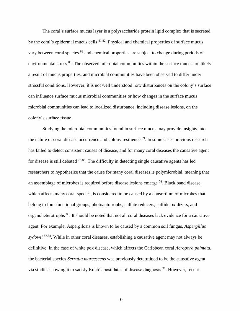
evenness than disease samples. For taxonomic composition, we found that sample type had a

significant interaction with season (R2 = 0.2, p-value = 0.001) (Table 2.5), and we observed that

sample type was most associated with changes in dispersion of microbial communities in the

PCoA space (Figure 2.8). This can be interpreted as low dispersion and high dispersion sample

types having microbial communities in common, but high dispersion samples types (especially

diseased samples) additionally exhibit some unique microbial communities. The analysis of

variance using distance matrices revealed a significant interaction between season and sample

type. Testing for such interactions is commonly advised as a first step, and if detected, then

further tests on main effects is not recommended 121.

20

Seasonal Samples

Of the 55 samples, 17 were collected in the spring, 25 were collected in the summer, and

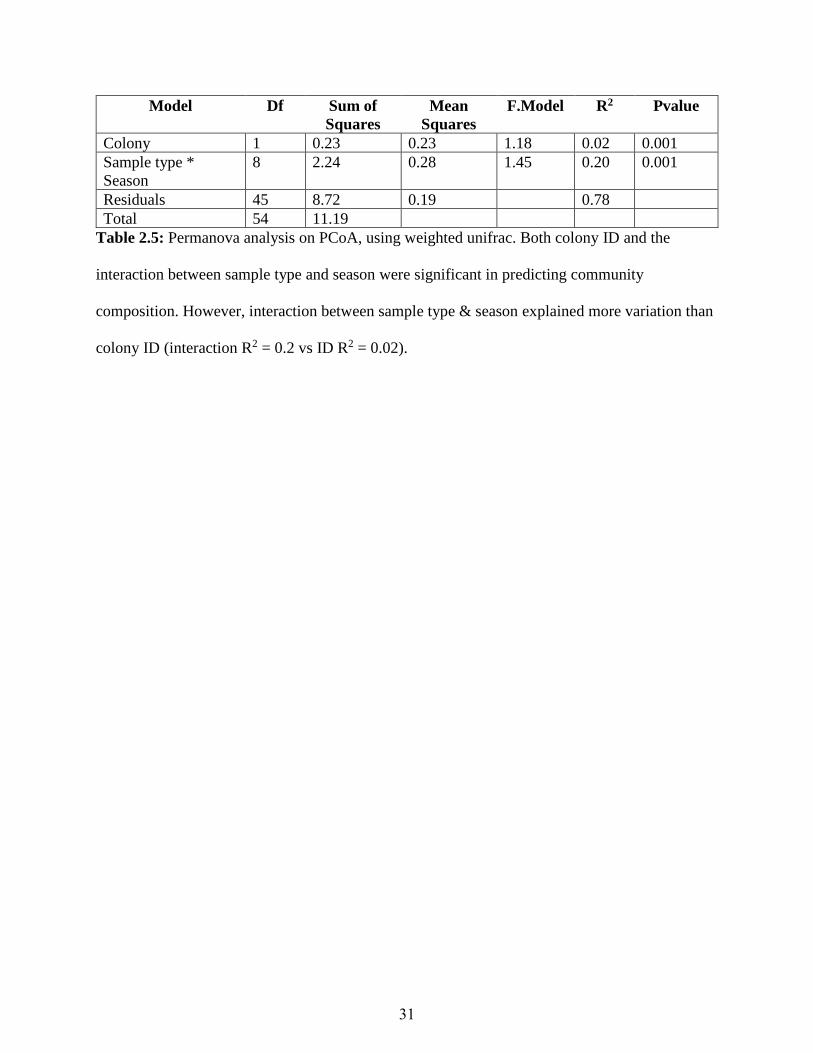
13 were collected in the winter (Table 2.1). Species richness was significantly different between

Spring – Winter and Summer -Winer (Figure 2.3). Shannon – Weiner values were strongly

significantly different between Spring – Winer and Summer – Winter (Figure 2.5). Species

evenness was also statistically significant between Spring – Winter and Summer – Winter

(Figure 2.7). For taxonomic composition, we found that season interacting with sample type to

be significant and provided predictive influence for taxonomic composition (R2 = 0.2, p-value =

0.001, Table 2.5). Season is predominantly associated with changes in centroids of microbial

clusters, but not dispersion (Figure 2.8). This can be interpreted as each season being associated

with relatively distinct microbial communities, but no season has more variation in microbial

community structure than any other season. As noted above, the analysis of variance using

distance matrices revealed a significant interaction between season and sample type and

consequently separate tests on main effects were not performed, as per recommendations of

developers of this technique 121.

Discussion

Increased diversity in disease samples

Samples taken from white pox lesions had a significantly higher microbial species richness

compared to other samples, and in particular samples taken from healthy tissue (Figure 2.2). This

is the first study that demonstrates this relationship for white pox disease. A previous study

involving white pox disease have failed to detect community differences between healthy and

diseased samples 107. However, studies of other coral diseases have also reported increased

21

microbial diversity in diseased samples. For white plague type II, multiple studies have observed

increased surface mucus layer diversity in diseased samples compared to healthy samples 123–125.

Increased diversity in surface mucus layer communities have also been observed across other

coral disease systems such as white plague (different from white plague type II), yellow band,

and black band 124–127. The equivocal nature of results to date across various coral systems invites

further studies, as we have performed, to begin to develop a broader understanding of how and

why microbial communities may differ as a function of disease status. There are various

hypotheses regarding the increased microbiome diversity with disease presence. Plausibly, the

surface mucus layer might be altered, either directly by invasion from the disease agent or

indirectly by environmental stress 123. Alternatively, the disease itself may be somewhat

incidental and rather the physiological function of the coral colony may change due to an

environmental stress event that results in change in surface mucus layer via mucus production

123. These hypotheses describe potential biological mechanisms for the observed trend, with the

caveat that variation in experimental protocols may also explain some differences between

studies 47,128.

Importance of season in difference for coral microbiome.

Seasonality and sample type were found to interact in terms of explaining microbial

community clustering based on community distance metrics. We found that seasonality tends to

generate distinct microbial communities where the variation associated with seasons is roughly

the same, whereas sample type was often associated with a subset of shared microbial

communities and some sample types having few unique communities (e.g., bleached samples)

and some sample types having many unique communities (e.g., disease samples). Temporal

changes in surface mucus layer communities have been observed in previous studies 129–131.

22

However, most studies have focused on relationships between community structure and stressors

that appear over time, such as coral bleaching and disease, rather than the direct influence of

seasonality. For the critically endangered elkhorn coral, there is a pressing need to classify stable

and transient members of the surface mucus layer communities 47, which have been shown to

affect both coral health and survivorship, and to establish how this distinction between these

factors correlate with colony health. Understanding how seasonal factors drive changes in

microbial community structure is an important component to answering this question, as white

pox disease in elkhorn coral has a seasonal signature, with disease common in summer and

occasionally spring, but not winter. Our results provide evidence that seasonality plays an

important role in governing the microbial communities of elkhorn coral populations and that

diseased colonies often exhibit distinct microbial communities, including having higher species

richness, having higher evenness than bleached coral samples (i.e., disease samples tend to not

be dominated by certain taxa) and exhibiting many unique communities compared to any other

sample type determined by community distance metrics.

Coral Bleaching

Bleached coral samples had, on average, the lowest diversity. However, the difference

between bleached and healthy corals was not statistically significant. A recent study examining

surface mucus layer communities in bleached and healthy Porites lobata found the communities

to be strikingly similar across sample types 132. However, in another study, researchers

demonstrated a change in microbial communities associated within coral tissue during bleaching

conditions 99. It is likely that the differences between these two studies can be partly explained

by what portion of the coral the sample was collected from. The surface mucus layer operates as

a protective barrier that interfaces between the coral and seawater. Corals are typically constantly

23

producing surface mucus which would lead to a high rate of turnover in microbial communities

81. Indeed, researchers have observed lower abundance and diversity in surface mucus layer

samples when compared against microbial samples collected from tissue 133. We found that

bleached samples did vary considerably from diseased samples, in terms of richness, evenness

and dispersion in the space measuring community structure distance.

The similarity between bleached samples and healthy samples, and the difference

between bleached samples and diseased samples sets up a scenario where tissue-associated

microbial communities may change disproportionately in terms of diversity and abundance under

stressful conditions compared to surface mucus layer communities, whereas surface mucus layer

communities are likely to more closely resemble surrounding seawater due to constant turnover,

but may change considerably when diseased.

Similarity between coral mucus and sea water

Seminal work related to the diversity of coral-associated microbial communities found that

coral microbial communities were more diverse when compared to surrounding seawater 74,134.

However, these initial studies focused on sampling coral tissue and did not isolate surface mucus.

Studies investigating diversity from mucus samples have found mucus – seawater samples to be

less distinct than tissue – seawater samples 130,135. Multiple studies have investigated the diversity

of surface mucus layer for A. palmata and have provided conflicting evidence regarding diversity

differences between mucus and seawater. One study, examining exclusively healthy coral, found

a distinct separation between surface mucus layer samples and sea water 108. While another study

investigating microbial communities for A. palmata affected by white pox disease failed to detect

significant differences between sea water and mucus samples, but researchers did detect a

difference between mucus and tissue samples 107. One explanation for the reported differences

24

could be due to sampling during healthy, Kemp et al. (2015)108, and stressed, Lesser et al.

(2014)43, conditions as evidenced by the observation of healthy and diseased colonies.

Additionally, contrasting finding may be partly attributable to the methodological differences

between the two studies.

Taxonomy

Members of the Synechococcaceae family were the most abundant taxa we observed across

the majority of our samples (Figures 2.9 and 2.10). Synechococcacea has been found in the

mucus samples for multiple species of coral sampled in the Florida Keys 135. Other studies have

shown that their abundance is typically higher during the summer when waters are warm 136.

Synechococcus species have been recovered from coral mucus samples elsewhere, and

researchers have speculated that Synechococcus could serve as a source of nitrogen for the coral

137,138. We observed Synechococcus to be most abundant in our bleached samples. This

observation, paired with previous speculation, suggests that the coral may be more reliant on its

microbiota for nutrients during periods of stress, because this family is plausibly of elevated

importance in such events. The second most abundant taxa were Pelagibacteraceae (Figures 2.9

and 2.10). The family Pelagibacteraceae has been speculated to be a member of the core

microbiome for multiple Caribbean coral species 139. In our diseased samples we observed an

increase in abundance of Rhodobacteraceae (Figure 2.9). An increase in Rhodobacteraceae has

generally been associated with diseased mucus samples 140.

Conclusion

Our detailed study of the microbial community diversity associated within the surface

mucus layer provides a better understanding of the differences between healthy, bleached, and

diseased colonies of A. palmata. Furthermore, by looking at associated communities through

25

time we have characterized how associated microbial communities vary seasonally47. Here we

present evidence that suggest the previously observed homogenous microbial community of

health populations can be disrupted by disease108. We anticipate that future studies may develop

the spatial and temporal scale of our study to better understand the dynamics of change in

microbial communities within and between reefs, and across a temporal backdrop of climate

change to evaluate the extent to which disease causes disruption to the mucus microbial

community. As our seasonality study was based on one year, longer term studies will be able to

clarify if there are yearly cycles in the microbial community or if the communities are constantly

moving through new states.

26

Table 2.1: Summary of samples, numbers, sequence depth and diversity. Diversity measures are

determined after rarifying the data to the minimal observed OTU within the whole data set

(minimal observed OTU = 1270). Numbers within brackets indicate standard errors.

Sample

Type

Sample

Number

Sequence

Depth

Chao1 Shannon -

Wiener

Pielou’s

Evenness

Sea Water 10 9195.7

(1874.27)

482.61

(32.89)

4.37 (0.12) 0.80 (0.01)

Healthy

Coral

26 9155.04

(1313.95)

482.52

(18.1)

4.28 (0.06) 0.76 (0.01)

Bleached

Coral

11 9534.91

(983.23)

454.63

(35.48)

4.2 (0.09) 0.74 (0.01)

Diseased

Coral

8 9022.875

(1177.91)

632.39

(45.63)

4.33 (0.18) 0.77 (0.02)

Season

Spring 17 7866.471

(876.21)

515.18

(34.05)

4.23 (0.09) 0.75 (0.01)

Summer 25 9422.36

(715.68)

473.04

(24.3)

4.08 (0.05) 0.76 (0.01)

Winter 13 10597.385

(2595.53)

505.75

(24.0)

4.53 (0.06) 0.80 (0.01)

27

Table 2.2: Linear mixed model performance for species richness Chao1 values as a function of

sample type and season ( with and without an interaction term) and with colony ID as random

effect. Models are compared with ANOVA. P-value < 0.05 indicates that the interaction between

sample type and season was not significant. Suggesting that there is no interaction between

sample type and season with respect to Chao1.

Model Df AIC BIC Log

Likelihood

Deviance Chisq Pvalue

No interaction 8 665.89 681.95 -324.94 649.89

With interaction 11 667.75 689.83 -322.87 645.75 4.13 0.25

28

Table 2.3: Linear mixed models for the microbial community Shannon-Wiener diversity index

as a function of sample type and season (with and without an interaction term) and with colony

ID as random effect. Models are compared with ANOVA. P-value < 0.05 indicates that the

interaction between sample type and was not significant. Suggesting that there is no interaction

between sample type and season with respect to Shannon-Wiener.


Likelihood


No interaction 8 27.17 43.23 -5.58 11.17


29

Table 2.4: Linear mixed models for Pielou’s J explained by sample type and season (with and

without an interaction term) and with colony ID as random effect. Models are compared with

ANOVA. Pvalue < 0.05 indicates that the interaction between sample type and was not

significant. Suggesting that there is no interaction between sample type and season with respect

to Pielou’s J.


Likelihood


No interaction 8 187.59 171.53 -101.80 203.59


30

Model Df Sum of

Squares

Mean

Squares

F.Model R2 Pvalue

Colony 1 0.23 0.23 1.18 0.02 0.001

Sample type *

Season

8 2.24 0.28 1.45 0.20 0.001

Residuals 45 8.72 0.19 0.78

Total 54 11.19

Table 2.5: Permanova analysis on PCoA, using weighted unifrac. Both colony ID and the

interaction between sample type and season were significant in predicting community

composition. However, interaction between sample type & season explained more variation than

colony ID (interaction R2 = 0.2 vs ID R2 = 0.02).

31

Figure 2.1: Distribution of sequencing depth for each sample prior to rarefaction. Here,

sequencing depth for the majority of samples is distributed around 8,000 read counts per sample.

Outlier read counts are of values 34,214 and 23,999. The minimum read count was 1270.

32

Figure 2.2: Estimated species richness (Chao1 values) by sample type using rarefied data.

Samples collected from white pox lesions typically exhibited higher species richness compared

to other sample types when compared with Tukey’s honest significance test.

33

Figure 2.3: Estimated species richness (Chao1) by season using rarefied date. Species richness

was observed to be typically higher during the winter. Richness values observed were

statistically different between Spring – Winter and Summer -Winter but not for Spring –

Summer, using Tukey’s honest significance test.

34

Figure 2.4: Shannon-Wiener index values by sample type using rarefied data. Shannon-Wiener

index values were statistically significantly different between sea water and healthy samples,

using Tukey’s honest significance test.

35

Figure 2.5: Shannon-Wiener index values by season using rarefied data. Shannon-Wiener index

values were statistically significantly different between Spring – Winter and Summer -Winter but

not Spring – Summer, using Tukey’s honest significance test.

36

Figure 2.6: Pielou’s J values by sample type using rarefied data. Pielou’s J values were

statistically significantly different between sea water – healthy and white pox – bleached, using

Tukey’s honest significance test.

37

Figure 2.7: Pielou’s J value by season using rarefied data. Pielou’s J values were statistically

significantly different between Spring – Winter and Summer -Winter but not Spring – Summer,

using Tukey’s honest significance test.

38

Figure 2.8: PCoA of all samples identified by (A) season and (B) sample type, with position

determined from rarified data set (rarified to minimum OTU observed in a sample, n=1270).

Distance matrix was determined using UniFrac method.

39

Figure 2.9: Abundance of taxonomic groups of microbes (at the family level) grouped by

sample type, using the non-rarefied data set.

40

Figure 2.10: Abundance of taxonomic groups of microbes (at the family level) grouped by

season, using non-rarefied data.

41

CHAPTER 3

INVESTIGATING THE IMPORTANCE OF LOCAL SPATIAL STRUCTURE AND

COLONY SIZE IN THE TRANSMISSION OF WHITE POX2

2 Griffin AP, Park AW. To be submitted to The American Naturalist.

42

Abstract

For decades, disease outbreaks across Caribbean coral reefs have significantly reduced

populations of important reef building coral. However, despite their frequent occurrence and

demonstrable impact, we still have limited knowledge of coral diseases, especially their local

transmission within a reef. Using surveillance data collected during an outbreak of white pox

disease at Looe Key Reef, FL, we evaluated several plausible hypotheses for local transmission

of disease. Our analyses provide evidence that local spatial structure is important in the

transmission of white pox disease, but incomplete data preclude us from singling out a

transmission mechanism. Accordingly, we developed an additional simulation study to

investigate how various sources of data incompleteness influence our ability to recover the true

transmission model. The statistical framework developed here can be adapted to other systems to

enhance our understanding of coral disease transmission more generally.

Introduction

Over the last several decades, researchers have observed precipitous declines in the abundance,

distribution, and function of coral reef ecosystems 7,20,21,23. Globally, degradation of coral reefs

has been attributed to a variety of factors, including eutrophication (which promotes overgrowth

of coral by algae 141,142) and increased temperature (which leads to coral bleaching 22,24). Some

corals also have experienced high mortality due to pathogens. Indeed, the incidence of disease

has been both more frequent and more severe in recent years 143. For example, the reef-building

coral Acropora palmata was almost extirpated from the Florida Keys National Marine Sanctuary

32. The loss of this important branching coral has contributed to the regional decline of complex

three-dimensional structure, which can significantly hinder a local reef’s ability to recover from

43

disturbance events 7,144,145. In the Caribbean, symptoms of disease have been reported in the

scientific literature since the late 1970s 37. However, despite widespread occurrence, severity,

and high level of incidence, the processes governing how pathogens that cause coral diseases

spread within reefs is poorly understood.

Local spatial structure is known to drive transmission in other sessile organisms 146,147.

For example, by analyzing the spatial point pattern of infected and severely infected sea fan coral

researchers observed that infected sea fans formed clusters at characteristic spatial scales,

supporting the notion of local contagious spread 54. Another study found evidence that a water-

borne transmission model for black band disease, whereby the pathogen is shed into the

environment by infected colonies, performed better at explaining patterns of local disease

transmission than a model that considers direct contact, where new infected corals are located in

close proximity, approximately 2mm, to previously infected corals 56. In a study for white-plague

disease, newly infected colonies were more likely to occur near colonies that were infected in the

previous survey 148.

In addition to local spatial structure, susceptible host size can also contribute to the

probability of a colony becoming infected. Given that marine pathogens frequently must persist

in the environment outsides of hosts, we suspect that individual colony size could influence local

pathogen transmission due to larger colonies serving as bigger targets for the pathogen to come

in contact with. Evidence for colony size has been observed in several coral disease systems. In

sea-fans, Jolles et al. (2003) observed disease prevalence was higher in larger sea fans and that

disease was more clustered in larger sea fans than smaller ones. In Puerto Rico, field surveillance

of yellow band disease was shown to disproportionately affect colonies larger than 50 cm 65. In

A. palmata, colony size was observed to be a significant predictor of incidence of white pox

44

disease 64. Thus, available evidence suggests that both host size and spatial structure help explain

local pathogen transmission among coral colonies, with the caveat that older colonies are

typically larger and may have had more time to acquire infection. This means that some caution

must be exercised when invoking the role of colony size, per se. However, in the white pox

system, the disease typically disappears in the winter, and therefore infection is unlikely to be

disproportionate in older colonies unless age affects an unmeasured physiological trait that

relates to susceptibility.

The classical approach to modeling infectious disease dynamics assumes that the host

population has homogenous mixing 11, whereby contact between individuals is random. This

characterization of random contacts between individuals in models may artificially increase the

speed of spread compared to natural, spatially-structured systems. Adopting a spatial framework

for modeling coral disease dynamics can encompass the observed importance of inter-colony

distance and more realistic patterns of pathogen transmission. One such framework, arguably the

ancestor of the approach used here, is a metapopulation approach, where classically there are

multiple, distinct populations of hosts that are connected by dispersal. In recent decades there has

been considerable progress in the integration of metapopulation dynamics and pathogen

transmission. Example case studies, such as measles virus in humans 149 and distemper virus in

seals 150, incorporate the discrete nature of populations coupled by movement of individuals

between populations. With spatially structured populations, these models can more accurately

describe the transmission dynamics 13 and the probability of long-term pathogen persistence in

affected populations 150. Within coral reefs, we can apply a similar logic where we consider the

reef as a metapopulation composed of discrete colonies. Colonies may be infected or uninfected,

45

and production of infectious propagules on a colony can cause transmission at other colonies. In

this way a colony is treated like a subpopulation in a metapopulation system.

This framework for modeling the spread of infectious disease introduces the notion of the

strength of coupling between two sub-populations. While coupling can be hard to measure

directly, models can incorporate realistic heterogeneity by including, for example, relevant

information on the sub-population sizes along with spatial structure. An example of this was

demonstrated with a measles epidemic in the UK 13, which implemented a ‘gravity’ model. The

term ‘gravity’ comes from the planetary analogy in which the gravitational force between two

planets is related to the product of their masses and inversely related to the distance between

them. Using spatially-resolved demographic and epidemiological data, Xia et al. (2004)13

estimated coupling between sub-populations via the product of the two sub-population sizes

divided by their distance. This was shown to be a statistically superior model compared to

models that made more simplistic assumptions about the degree of coupling between sub-

populations. More recently, this approach has been extended to a generalized gravity model to

explain the spread of the fungal pathogen that causes white-nose syndrome in bat populations

and the spread of Ebola in West Africa 151,152. With these models, populations are represented as

nodes in a network, and a generic function is used to characterize the probability (p) that a

susceptible node i escapes infection from an infected node j in a fixed time interval:

𝑝𝑖𝑗 =1

1 + 𝑒−𝑓 (1)

The function smoothly varies between 0 and 1, and the component f can be a function of

different spatial, demographic or environmental traits. The pattern of nodes switching from

46

uninfected to infected over time as a result of pairwise interactions between nodes may be

described in an exact likelihood expression 152,153. The component f can then be modified to

represent different rules for transmission. Each modified f component is a different model that

represents a hypothesis for pathogen transmission. This approach allows the models to be

competed against one another to determine which model best explains the observed data.

In contrast to well-studied plant and animal populations, the spread of pathogens in coral

populations is relatively under-developed. Given the sessile nature of corals and the evidence

that colony size is important to transmission, we develop and test a set of generalized gravity

models to explain the spatial dynamics for a local outbreak of white pox disease. While our

version is closely related to gravity models described above 152,153, we assume that nodes are

individual colonies, with the distance between pairs of susceptible and infected colonies and the

sizes of the two colonies potentially influencing transmission: i.e., via the function, f, in Eq. 1. In

classic metapopulation gravity models, subpopulation sizes are important as they link locations

by dispersal of individuals. Here, we assume that colony sizes are important because large

infected colonies may produce more infectious propagules than small infected colonies, and

large susceptible colonies may provide larger targets for infectious propagules, compared to

small susceptible colonies.

The spatiotemporal data for white pox disease dynamics lend themselves to integration

with the generalized gravity modeling framework to assess if and how inter-colony distance and

colony size contribute to transmission risk. Accordingly, we construct and analyze seven

different models for white pox disease transmission at the reef scale and determine which models

provide the best fit to the empirical data set. The competing models represent various biological

47

hypothesis, explained below, that express how white pox disease may be transmitted between A.

palmata colonies within a reef.

Methods

Data Collection

Researchers visited Looe Key reef during in 2009 in June, July, August, and September. Looe

Key reef is located at (24° 32′ 51″ N, 81° 24′ 24″ W) inside the Florida Keys National Marine

Sanctuary (FKNMS). The initial month was selected as part of a seasonal survey for disease, and

researchers decided to conduct follow-up surveys after a severe outbreak was detected. Each

month researchers, using SCUBA, documented the health status of individual A. palmata

colonies. Colonies were determined to be either infected or uninfected by the presentation of

characteristic symptoms of white pox disease, consisting of irregularly shaped white blotches

distributed across the coral surface. Surveyed colonies were photographed for reference, and a

scale ball was placed in the field of view to facilitate measurement of colony surface area and

lesion size. Colony size was then measured via photography analysis using imageJ (version 1.47)

to estimate the projected surface area for each colony. Colony position was determined by

measuring the distance and bearing of the colony center from a reference stake. Due to erratic

extreme weather events, some surveys were terminated early, leaving the health status of certain

colonies unknown.

Competing Hypotheses for White Pox Disease Transmission

General Probability Function and Likelihood expression

The general functional form for the probability that a healthy colony escapes infection by

an infected colony in a fixed time interval, equation (1), forms the building block for the

expression for the likelihood of observing a data set. At each time point, t, the set of source

48

(infected) colonies, j, were identified as those infected at the previous time point, t-1, and

uninfected target colonies, i, were grouped into two subsets: ‘i1: becoming infected at time t’ and

‘i0: remaining uninfected at time t’. Consequently, the likelihood of the observed events at time

t is the product of the probability that i0 colonies escaped infection from all j sources multiplied

by the probability that all i1 colonies were infected by at least one j source. These two

probabilities can be further expanded based upon Eq. 1. We let pij be the probability that

colony j fails to infect colony i at time t, with the form of pij given by the transmission models in

Table 1. For convenience, we estimate the probability of escaping infection because it is easier to

determine the probability of escaping all infected colonies rather than considering the probability

of becoming infected from all possible combinations of infected colonies. To accommodate these

properties, the data were coded as surveillance-date records of infection status (infected: y = 1;

uninfected: y = 0) and fitted to minimize the negative log-likelihood of observing the full dataset

across time points:

− ∑ log {∏ {1 − ∏ 𝑝𝑖1𝑗

𝑗

} × ∏ {∏ 𝑝𝑖0𝑗

𝑗

}

𝑖0𝑖1

} (2)𝑡

This approach allows us to determine the likelihood of each candidate model and thus

determine the AICc for each model in describing the outbreak of white pox disease at Looe Key.

We compared 7 different models, which varied in the functional form of the expression f, in

Equation 1. The various functional forms for f are summarized in Table 1 and differed in whether

they included effects of distance, the size of the susceptible colony, and/or the size of the colony

that was the potential source of the disease. We next briefly describe each of these models.

Reduced Null

A reduced null model which simply assumes a fixed probability (q) of infection, per

sampling interval, regardless of prevalence (i.e., a non-contagious process) was calculated as the

49

likelihood of the binomial event in which each infected colony that first remains uninfected for t

time periods contributes q(1-q)t to the overall likelihood and each colony that never gets infected

contributes (1-q)T to the overall likelihood, where T is the total number of time periods in which

infection could occur. This provides a fixed probability of becoming infected. This reduced null

model is included for completeness. However, because it is of a different form to the other

models (considering intrinsic colony infection risk, versus escaping contagious infection from

other colonies) it does not have an equation for f. Relatedly, comparison with other models (via

likelihood and Δ AIC) is provisional because the reduced null model fit is based on a different

amount of data. The maximum likelihood estimate for q is simply the ration of number of times

an infection event occurred to the number of times an infection event could have occurred.

Null Model

The main null model represents a general probability of escaping infection in which all

infected-susceptible colony pairs are considered to be equivalent (and not dependent on their

relative positions or sizes). For this model, f is represented only by the parameter 𝛽0. Because

this null model has a fixed probability of escaping infection (i.e., assuming a contagious

process), it means that when there are many infected colonies the overall probability of escaping

infection is lower than when there are few infected colonies.

Colony Size Model

The colony size model represents the scenario that the size of the uninfected colony

affects its probability of becoming infected. Similar to the null model, the general probability

function is modified to estimate the probability that colony i becomes infected. For this model, f

takes the form of 𝛽0 + 𝛽1 ∗ 𝑆𝑖 where 𝛽0 is the parameter defining a baseline probability of

infection, and 𝛽1represents the additional contribution of a unit increase in uninfected colony

50

size. The sign of 𝛽1 indicates if larger colonies are more (𝛽1>0) or less (𝛽1<0) likely to become

infected.

51

Spatial Diffusion Model

The spatial diffusion model represents the scenario where inter-colony distance (dij)

influences the probability that an uninfected colony escapes infection from infected counterparts.

The phrase ‘diffusion model’ is widely used in the gravity modeling literature and relates to

particles undergoing diffusion such that they are more likely to travel relatively short vs. long

distances in a fixed time interval. For this model, f takes the form of 𝛽0 + 𝛽1 ∗ 𝑑𝑖𝑗. Here 𝛽0 is a

parameter defining a baseline probability of infection, and 𝛽1 represents the additional

contribution of the distance between uninfected colony i and infected colony j.

Generalized Gravity Models

The generalized gravity model approach considers the interaction between the size and

distance of two objects. The interaction between two objects consists of the distance between

them divided by the product of their sizes.

Generalized Gravity Model 1

Generalized gravity model 1 considers the distance between two colonies, infected and

susceptible, and the size of both colonies. Biologically, the size of the infected colony could lead

to more pathogen shedding in the environment while the size of the susceptible colony would

provide a larger target for free-floating pathogens. For this model, f takes the form of 𝛽0 +

𝛽1∗𝑑𝑖𝑗

(𝑆𝑖∗𝑆𝑗)𝛽2. Here 𝛽0 is the parameter defining a baseline probability of infection, 𝛽1 represents the

parameter for the distance between colony i and colony j, and 𝛽2 represents the parameter for the

contribution of the size of both colony i and colony j.


52

Generalized gravity model 2 considers the distance between two colonies and the size of

only the uninfected colony i. Biologically, this would mean that only the size of the susceptible

colony is important in pathogen transmission (a large target). For this model, f takes the form of

𝛽0 +𝛽1∗𝑑𝑖𝑗

𝑆𝑖𝛽2

. Here 𝛽0 is the parameter defining a baseline probability of infection, 𝛽1 represents

the parameter for the distance between colony i and colony j, and 𝛽2 represents the parameter for

the contribution of the size of only colony i.


Generalized gravity model 3 considers the distance between two colonies and the size of

only the infected colony j. Biologically, this would mean that larger colonies would be shedding

more pathogens into the environment, but susceptible colony size is not important for

transmission. For this model, f takes the form of 𝛽0 +𝛽1∗𝑑𝑖𝑗

𝑆𝑗𝛽2

. Here 𝛽0 is the parameter defining a

baseline probability of infection, 𝛽1 represents the parameter for the distance between colony i

and colony j, and 𝛽2 represents the parameter for the contribution of the size of only colony j.

Colony-Size-Independent Model

The last model, colony-size-independent, considers how the distance between colonies

and the size of the colonies independently contribute to the probability that colony i escapes

infection. It is more in the spirit of the language of generalized linear modeling. Biologically,

both size and spatial structure are important for disease transmission. However, there isn’t a

gravity interaction between large and small colonies. For this model, f takes the form of

𝛽0 + 𝛽1 ∗ 𝑑𝑖𝑗 + 𝛽2 ∗ 𝑆𝑖𝑗 Here 𝛽0 is the parameter defining a baseline probability of infection, 𝛽1

53

represents the parameter for the distance between colony i and colony j, and 𝛽2 represents the

parameter for the contribution of the size of both colony i and colony j (in product form).

Using Maximum Likelihood and AICc to evaluate competing models

Estimating Likelihood

A maximum likelihood approach was adopted for parameter estimation. The maximum

likelihood method determines the best combination of parameter values for a specified model

that maximizes the chances of observing the data. For each model, the initial estimation method

used the Nelder-Mead algorithm for optimization (also known as downhill simplex). The Nelder-

Mead method initially covers a wide area of parameter space that heuristically reduces the size of

the simplex with each iteration. A drawback to Nelder-Mead is that is it susceptible to finding a

local minimum and does not necessarily thoroughly explore global parameter space. Conversely,

simulated annealing is a global optimization method that probabilistically jumps around

parameter space. This jumping helps increase the chances of finding a global minimum and

reduces the chances of getting stuck in a local minimum. However, simulated annealing can be

difficult to implement when the parameter space is not discretely defined. The estimation

procedure was an integration of both methods by first optimizing locally with the use of Nelder-

Mead 152, then estimating parameters with simulated annealing using local estimated parameters

from Nelder-Mead as an initial condition 152. Local optimization, Nelder-Mead, was run before

global, simulated annealing, due to the parameter space not being well defined or discrete. The

Broyden–Fletcher–Goldfarb–Shanno, BFGS, algorithm was used for estimating the null model

parameter because the null model only has one parameter being estimated.

Evaluating Model Performance

AICc

54

Akaike information criterion, adjusted for small sample sizes, AICc, was used to evaluate

model performance:

𝐴𝐼𝐶𝑐 = −2𝑙𝑛(𝐿) + 2𝐾 +2𝐾(𝐾 + 1)

(𝑛 − 𝐾 − 1) (4)

Where K represents the number of parameters in the model, L represents the estimated likelihood

for that model, and n is the number of uninfected coral colonies. To compare AICc values with

the best fit model, Δ AICc values were calculated:

∆𝐴𝐼𝐶𝑐 = 𝐴𝐼𝐶𝑐 − min (𝐴𝐼𝐶𝑐) (5)

Models within 2 ΔAICc units were not considered demonstrably different in their relatively

quality.

Censored Colonies

The health status of certain colonies was unknown at certain points during the survey

(Figure 3.1). Permutation sets, containing all possible scenarios of infected / uninfected for

censored colonies, were generated to account for the censorship of colony health status. The

collective set of permutations accounted for all possible combinations of healthy and diseases

censored colonies. The negative log likelihood was determined for each permutation. The

average negative log likelihood can be considered as the sum of estimated negative log

likelihoods divided by the number of permutations. The average negative log likelihood is the

value that is returned from the estimation procedure.

Goodness of Fit

A stochastic simulation was conducted with the best-fit model to evaluate how the best fit

model performs in terms of generating data similar to the observed data. The simulation

incorporated the best-supported model (i.e., the spatial diffusion model: see Results) to simulate

55

an epidemic over three months. Initial conditions for simulation were determined based on a

colony’s observed health status in the first month of surveillance. Status was determined with a

weighted binomial distribution for colonies that were censored during the first month. The

binomial weight was calculated as the observed proportion of infected colonies. After

determining the initial conditions, the model parameters were then used to simulate the next

three observed months of the epidemic. For each month, the model determined the infection

status of each colony, and from this, it calculated the probability of becoming infected for each

healthy colony. A weighted binomial draw was then performed for each healthy colony using its

unique probability of becoming infected. In total, we generated ten initial condition sets due to

the uncertainty in censored colonies and simulated each set ten times, for a total of 100

simulations. When then compared the observed cumulative prevalence from field observations

with the cumulative prevalence from simulations as a measure of goodness of fit.

Simulating White Pox Disease Epidemics

For many marine systems, diseases are often considered caused by opportunistic pathogens

that can emerge with little warning. We experienced these challenges when conducting

surveillance for white pox disease and almost always missed the onset of white pox epidemics.

Missing the initial outbreak period often resulted in many missed opportunities for observing

disease transmission. Given these challenges, we developed a simulation for white pox dynamics

to assess if our approach could recover the model that generated the data. Our experimental

design first establishes how well maximum likelihood detects the generating model.

Furthermore, we wanted to recreate scenarios often encountered with surveillance data from

56

marine diseases. We accomplished this by degrading the generated data in multiple ways (Figure

3.1) and exploring how the degraded data can influence the initial model results.

Rationale

The empirical data fitting exercise ultimately led to some equivocal results. This was

considered to be due to limitations of the data set: 1) approximately 2/3 of the observed colonies

for the first month were infected with disease, giving limited ability to observe new infections; 2)

20% of the colonies were not observed in any month, further limiting the opportunities for

observing transmission; and 3) we only observed one outbreak of disease in one local population.

To assess how our general approach is impacted by these data limitations, we developed a

simulation model that generated a white pox disease outbreak. We then degraded the quality of

simulated data by censoring the infection status of certain colonies. We identified four different

types of censorship we believed might limit model performance, and that reflect issues typically

encountered when working with surveillance data from the marine environment.

Simulation Approach

The developed model simulated a white pox outbreak occurring over several time steps,

using the diffusion model and colony spatial structure (ultimately, two reasonably well-supported

models) and demographic population data (number, size and location of colonies) from the 2009

summer surveillance at Looe Key reef. We ran the model for ten-time steps. We used the

parameters estimated from the observed epidemic as a starting point. We then found our new

parameters by finding a parameter set that typically resulted in an average cumulative prevalence

similar to field surveillance data.

57

Treatments for censoring simulated data

1) Random Censoring.

The first treatment represents a scenario in which a colony was not observed during a survey,

which would mean that its health status is censored. An explanation for why a colony went un-

observed could be because sudden changes in weather conditions resulted in an early termination

of the survey. With the simulated data, a colony and time point were chosen at random, then that

colony’s health status was changed from either healthy or infected to censored. Colonies were

exempted from censoring if they were the only infected colony for a given time point.

2) Colony Censoring

The second treatment represents a scenario in which a colony was never detected at a site but

contributed to transmission. This might occur when a colony was beyond the edge of the site

within a reef, but close enough to influence the probability of other colonies becoming infected.

A colony that was selected for complete censoring had its health status masked in subsequent

analyses (relative to control, in which the analysis was performed without masking).

3) Temporal Censoring

The third treatment represents missed opportunities for observing the spread of disease.

There is limited evidence to suggest how quickly a pathogen may spread during an outbreak

event. This means that researchers may have a mismatch between their frequency of surveillance

and the rate of spread. For this situation, we randomly selected time points during the disease

epidemic and masked them from data analysis (relative to control).

58

4) Initial censoring

Many marine pathogens are considered to be opportunistic and often emerge with little

warning 154. This leads to situations where researchers begin collecting outbreak information

well into the current epidemic. With the supply of susceptible individuals depleted, so are the

opportunities to observe the spread of disease, which could bias results. For this treatment, we

started recording the status of coral colonies after there was 50% disease prevalence in a given

simulation. 50% prevalence would be close to observed prevalence if we assumed all censored

colonies were uninfected.

Results

Disease Surveillance

During the summer of 2009, researchers followed an outbreak of white pox disease at Looe Key

reef, FKNMS, from June through September by visiting the study site each month and observing

the health status of 34 individual colonies (Figure 3.2). However, we occasionally missed a

colony during a survey. In the first month, seven (of 34) colonies were not surveyed. While in

the third month, one colony was again not surveyed, and another was lost due to mortality.

Disease incidence, new cases of disease, were highest in the initial survey with 19 cases of

disease. This diminished in each follow up survey to a minimum value of 3 new cases (Figure

3.3). Cases of white pox disease were observed in every month in this study, including the initial

observation, and the highest prevalence of disease was observed in July (Figure 3.4). Disease

prevalence averaged 72% for the first three months and dropped to 38% in the final month of the

survey. In the initial survey we observed that larger colonies were more frequently infected than

smaller colonies (Figures 3.5 & 3.6). From June to July, we observed 4 colonies became

infected while another 4 colonies became uninfected (Figure 3.2). From July to August, 2

59

colonies became infected while another 2 colonies became uninfected (Figure 3.2). From August

to September, 2 colonies became infected and 12 colonies became uninfected (Figure 3.2).

Through out all four surveys, 2 colonies were never observed to be infected and 5 colonies were

observed to be infected in each survey (Figure 3.2).

Empirical Fit

The spatial diffusion model (which did not include effects of colony size) provided the

best fit, based on AICc (Table 3.2), although the null model was also plausible (i.e.,

ΔAICc=2.78). This indicates that, at the very least, the prevalence at any point in time impacts

the probability of infection, and further, that local spatial structure is likely important for

pathogen transmission, though an extended data set (such as would be generated by catching the

inception of the epidemic) would be required at a reef of this population size to definitively

advance the hypothesis of transmission to near neighbors (i.e., the spatial diffusion model).

Additionally, the results from the reduced null model found that the NLL was 22.2, suggesting a

poor fit.

Goodness of Fit

Using parameter estimates from the best-fit model, we predicted that the pathogen is

expected to spread quickly, going from an initial prevalence of 65% in June to a prevalence of

95% in the next month, and progressing to 100% by September (Figure 3.7). However, the

observed cumulative prevalence is somewhat lower in the real data, although the trend is quite

similar.

Simulation

When simulating spread under the spatial diffusion model, the infection spreads from an

infected individual to nearby uninfected individuals. With the complete simulated data (no

60

censoring / data degradation), we observed that the maximum likelihood approach recovered

diffusion as the true model the majority of the time ( Table 3.4, Figure 3.8). It appears that three

of the data degradation patterns, random, colony, and temporal had limited influence on the

detection of spatial diffusion as the true mechanism ( Table 3.4). However, censoring the onset

of the epidemic did dramatically influence our ability to detect the true model, with no model

generating a superior fit compared to any other (Table 3.4).

Discussion

Intercolony Distance Contributes to Infection Risk

Confronting our models with observational data from an outbreak of white pox disease, we

found evidence that local spatial structure plays a role in transmission (Table 2). This extends the

limited evidence on transmission mechanisms in coral diseases; in a previous study, researchers

found that local spatial structure was also important in the contagious spread of white plague

disease in the Gulf of Eliat Red Sea 148. Evidence for local spatial structure suggests that reefs

may be differentially at risk following an index case, based on their density and colony

configuration. It is likely that as individual colonies are lost over time due to environmental

disruption, such as temperature stress and bleaching, reefs may be at a reduced risk from

contagious pathogens. Conversely, growing reef populations may become more vulnerable to

disease outbreaks as their demography transitions them to a denser status. Being unable to

observe the onset of the epidemic, impacted our ability to rule out alternative hypotheses,

particularly the prevalence-only null model.

Lack of detection of the effect of colony size

We were unable to detect any evidence that colony size contributed to infection risk

(Table 3.2). We anticipated that colony size would be important, as suggested by previous

61

research 64. The relatively poor performance of models containing information about colony

sizes could be due to missing the early onset of the epidemic, limiting the opportunity to observe

which colonies were driving the establishment of white pox disease. In the first month of

observation, an appreciable proportion of the larger colonies were observed to be already

infected (Figures 3.5 & 3.6). A high number of large colonies already infected would limit the

influence for any model that accounted for colony size.

Imperfect Goodness of fit performance

Compared to the observed trend, the goodness of fit simulations tended to over-predict

cumulative prevalence. The rate of infection in the model is determined by the parameter values

that were estimated with maximum likelihood. It is plausible that the estimation was limited by

the low sample size of surveillance data. One assumption in our model that could also explain

the overestimation of spread is that our colonies do not recover once they become infected.

Ignoring recovery allows infected individuals to build up over the course of the epidemic at an

inflated rate and increases the risk of susceptible colonies becoming infected, although recovery

is not common in the white pox disease system except on approaching winter conditions. In the

Looe Key 2009 data used here, recovery appears to occur on several occasions, particularly

toward the end of the epidemic, and accounting for this by correspondingly lowering the

observed prevalence actually leads to much better agreement between model-based and

empirical cumulative prevalence.

What we learned from our simulation approach

From our simulation, we found that many types of colony censoring had a limited

influence on detecting the underlying model (Figure 3.8). However, censoring the onset of the

epidemic did reduce the overall separation between models (Figure 3.8). When we first arrived at

62

our study site in June 2009, we found the outbreak to be well underway (Figure 3.3). The

observed prevalence was greater than 50% in our first survey (Figure 3.4). There were also

several colonies whose health status was unknown (Figure 3.2). The insight from our simulations

would suggest that missing the beginning of the epidemic explains the ensuing difficulty in

separating models, and the colony censoring from the first sampling month had little effect on

identifying the best fit model based on the provided data.

Importance of Coral Surveillance

This study highlights the need for a discussion regarding how to optimize field

surveillance for coral diseases. Our general insights suggest that field surveillance should ideally

include rapid surveys with minimal time lapses between observations 155 as is also advocated for

characterizing the rate of pathogen spread in other wildlife populations 156,157. However, this is

typically not the case with marine pathogens as many infections are believed to be opportunistic

by taking advantage of changing environmental conditions 158. This often leads to scenarios

where researchers and managers are challenged to make rapid decisions with incomplete

information. Having missed the early stages of an epidemic in the field, our simulation results

demonstrate how missing that initial period can influence the ability to detect transmission

mechanisms using statistical modeling. Beyond the key areas we have focused on, other

unexplored issues in coral diseases include understanding how pathogens spread at larger spatial

scales, especially between reefs, and if pathogens are capable of overwintering. Given the

practical constraints, our results suggest that coral disease surveillance be conducted just before

and during when the seasonal risk for disease incidence is high. Increased surveillance around

seasonal windows may be augmented by also identifying if there are seasonally-driven

63

environmental factors that are associated with disease outbreaks 53. This is a topic explored in

Chapter 4.

Considerations for other Gravity Models

Our data indicated that spatial diffusion was the best fit model to the provided data (Table

2). Maher et al. (2012) 151, studying the spread of a fungal pathogen affecting North American

bats, found support for a gravity model that included the number of bat caves as the size term.

The preferred model also included winter length as an environmentally related parameter, which

suggests that including environmental data in gravity models can improve performance once the

environmental predictors are well-characterize. When investigating the 2013 – 2015 Ebola

outbreak in West Africa, researchers found support for a gravity model, with population density

as a size term, to be the best-fit model describing the spread of Ebola across affected core

countries in Africa 152. The Ebola gravity model also included an extra parameter that accounted

for the border crossing security between countries, suggesting that barriers to spatial

transmission, perhaps based on current flow, could ultimately be included in models for the

spread of marine pathogens. In both white nose syndrome in bats and the Ebola outbreak in West

Africa, researchers observed that gravity models which included some form of size term. In our

study, we did not find support for gravity models including colony size but rather a simple

diffusion model, capturing transmission between relatively near neighbors. We may have missed

the time window in which colony size was exhibiting a strong influence on the local spread of

white pox (Figures 7 & 8). Alternatively, simple diffusion (transmission to near neighbors) may

adequately describe pathogen transmission causing white pox disease, but we believe more work

is necessary before ruling out the possibility of such gravity model type transmission in coral

disease systems.

64

Debating the importance of contagious spread for coral disease

Over the last decade, researchers have begun to question the nature of coral disease

transmission and two leading alternative hypotheses have emerged. One hypothesis assumes that

coral diseases spread contagiously from one individual colony to the next with the probability of

becoming infected being higher for nearby susceptible colonies 32. The hypothesis for contagious

spread has been supported by observed spatial clusters of disease54, either through indirect

(waterborne / vector ) or observed direct contact in experimental studies 159–161, and statistical

and theoretical models 57,148. The second hypothesis suggests that coral diseases are a result of

environmental conditions and opportunistic microbial communities and do not spread

contagiously 76. Support for non-contagious spread is primarily generated by the unknown

causative agents for many coral disease systems 162. However, researchers have also failed to

detect spatial clusters of infected colonies 85 and have been unable to induce transmission in

laboratory experiments 163. We examined a reduced null model in our system that assumed a

fixed probability of becoming infected, independent of reef-level prevalence. This simple model

did not provide a good fit to our data compared to models with any kind of contagious spread

(Table 3.2). However, in general, evidence for contagious and non-contagious spread in coral

disease systems highlights the complicated nature of conducting disease research in coral

communities. There is shared agreement in both camps that corals suffer from some form of

disease that results in decreased fitness for afflicted colonies and while etiologies of disease

maybe unresolved, there is agreement in the description for the symptoms of disease. Here, we

have provided a statistical framework that will allow researchers to better investigate the open

question concerning the nature of coral disease spread.

Conclusion

65

We have provided evidence that local spatial structure can be important in the

transmission and maintenance of an ongoing coral disease epidemic. However, our study is not

without limitations, and future studies will benefit from anticipating the challenges involved in

conducting field surveillance for coral diseases. More importantly, we have provided a statistical

framework that will allow researchers to better explore questions related to coral disease

transmission that accounts for the dynamics involving a disease outbreak. Furthermore, our

framework can be further adopted incorporate other potentially relevant factors for coral diseases

such as relevant environmental variables 153.

66

Table 3.1: The functional forms of the f term for equation 1. Parameter dij represents the distance

between uninfected colonies (i) to infected colonies (j). Si indicates the size of an uninfected

colony while Sj indicates the size of an infected colony, and Sij denotes the product of the sizes of

each. Each form (row) represents a different hypothesis for pathogen transmission at a local

scale. *For completeness, a reduced null model is included. Because it is of a different form to

the other models (considering intrinsic colony infection risk, versus escaping contagious

infection from other colonies) it does not have an equation for f. Relatedly, comparison with

other models (via likelihood and Δ AIC) is provisional because the reduced null model fit is

based on a different amount of data.

Model

Description of feature(s) that determine

probability of becoming infected f

Reduced Null Fixed probability applied each time

step

n/a*

Null

Only number of infected colonies 𝛽0

Colony Size

Size of uninfected colony 𝛽0 + 𝛽1 ∗ 𝑆𝑖

Spatial Diffusion

Inter-colony distance between infected

and uninfected colonies 𝛽0 + 𝛽1 ∗ 𝑑𝑖𝑗

Gravity 1 Size of infected and uninfected

colonies, and inter-colony distance 𝛽0 +𝛽1 ∗ 𝑑𝑖𝑗

(𝑆𝑖 ∗ 𝑆𝑗)𝛽2

Gravity 2

Size of uninfected colonies, and inter-

colony distance 𝛽0 +𝛽1 ∗ 𝑑𝑖𝑗

𝑆𝑖𝛽2

Gravity 3 Size of infected colonies, and inter-

colony distance 𝛽0 +𝛽1 ∗ 𝑑𝑖𝑗

𝑆𝑗𝛽2

67

Independent Size of infected and uninfected

colonies, and inter-colony distance –

with size and distance acting

independently

𝛽0 + 𝛽1 ∗ 𝑑𝑖𝑗 + 𝛽2 ∗ 𝑆𝑖𝑗

68

Table 3.2: Model performance values from estimating parameters with maximum likelihood.

Spatial Diffusion is determined to be the best-fit model with the nearest Δ AICc value being > 2

(Null model).

Model NLL AICc Δ AIC

Reduced Null 22.2 46.573 6.742

Null 20.218

42.61 2.77

Colony Size 19.694

43.934 4.1

Spatial Diffusion 17.643

39.832 0

Gravity -Targets

and Area

19.843 46.83 6.99

Gravity Sources

Area

18.754

44.651 4.82

Gravity Targets

Area

20.212

47.567 7.74

Size Space

Independent

20.191

47.525 7.69

69

Table 3.3: Estimated parameters for each model using maximum likelihood. Parameters are

defined for each model in Table 3.1.

Model 𝛽0 𝛽1 𝛽2

Null -3.68 NA NA

Colony Size -0.54 9.38 NA

Spatial Diffusion -1.98 -0.02 NA

Gravity -Targets

and Area -3.94 0.04 -2.09

Gravity Sources

Area -0.79 -0.04 1.59

Gravity Targets

Area -3.59 -11.14 1.26

Size Space

Independent -3.94 0.04 -2.09

70

Table 3.4: Model selection under data degradation scenarios. Number of times (out of 100) that

a model was preferred based on lowest AIC score. The true model was “Space” and was used to

generate the 100 sets of data (10 initial conditions and 10 replications per initial condition) for

which models were competed. Coral colony number, size and configuration was taken from the

Looe Key 2009 data. Several initial conditions were used because the health status of a subset of

colonies was censored at the first surveillance. In each initial condition set, each of these initially

censored colonies (n=7) was set to diseased using a binomial trial with probability taken from the

known prevalence at that time point.

Degradation Space Size Gravity

Complete

Gravity

Sources

Area

Gravity

Targets

Area

Size Space

Independent

Base 100 0 0 0 0 0

Censor 99 0 0 1 0 0

Delay 1 76 5 4 1 13

Random 99 0 0 1 0 0

Temporal 89 9 0 1 0 1

71

Figure 3.1: Schematic outlining the simulation approach and degradation of simulated epidemic

data. (A) ‘No censoring’ represents a full data set from simulated disease epidemic with 4

individual colonies and 5-time steps (not to scale: real data set has many more colonies) (B)

‘Random censoring’ of data leads to randomly selected colony-time combinations being

censored. (C) ‘Colony censoring’ selects a colony at random and censors its diseases status. (D)

72

‘Temporal censoring’ censors selected time points from the epidemic. (E) ‘Initial Censoring’

censors the initial onset of the epidemic.

73

Figure 3.2: Individual colony health status through time for summer surveillance 2009 at Looe

Key reef, y-axis indicates the unique colony ID while the x-axis indicates the month. Blue

indicates that a colony was observed to have an active lesion during the survey. White indicates

that no active lesion was observed on the colony during the survey. Grey indicates that a colony

was not surveyed (censored).

74

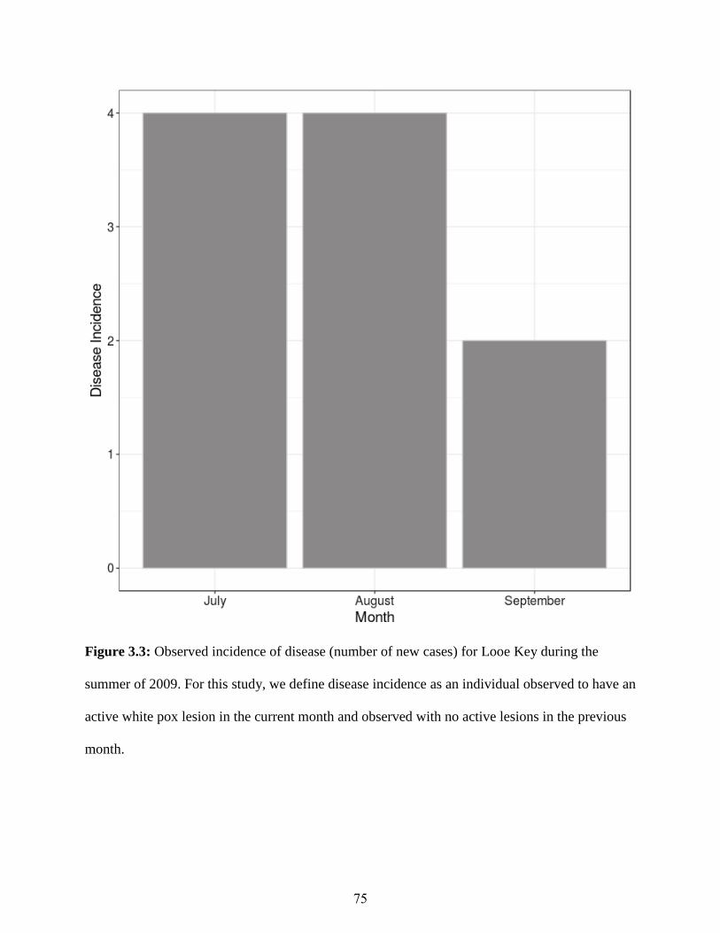
Figure 3.3: Observed incidence of disease (number of new cases) for Looe Key during the

summer of 2009. For this study, we define disease incidence as an individual observed to have an

active white pox lesion in the current month and observed with no active lesions in the previous

month.

75

Figure 3.4: Observed disease prevalence for each month from the survey. Disease prevalence

was determined using the health statuses for the colonies that were observed and did not include

any censored colonies. Disease prevalence is at a consistent level for the first three months

before a significant drop off in September.

76

Figure 3.5: Relationship between colony size and disease status (healthy / diseased) from the

initial month of our survey. Individual colonies observed to have active lesions were marked as

infected while no active lesions would mean that a colony would be healthy. A generalized linear

model with a binomial distribution was used to fit the provided trend line.

77

Figure 3.6: Differences between colony size and health status from the observed data in the

initial month of our survey. Individual colonies observed to have active lesions were marked as

infected while no active lesions would mean that a colony would be healthy. This figure excludes

an infected colony that is sufficiently large enough to be an outlier in terms of size for better

visualizing the general trend (infected, size = 7584 cm2).

78

Figure 3.7: Cumulative prevalence from our goodness of fit (Black lines) and the observed

cumulative disease prevalence (Red line). We see that disease prevalence increases the most

from June to July in both simulated and goodness of fit. However, disease prevalence is

consistently lower in our observed data compared to the simulated data indicating that

parameters estimated contribute to a fast rate of spread.

79

Figure 3.8: Results from simulating white pox disease events using Looe Key spatial structure

and colony size. AIC was used here over AICc due to the increase in sample size from the

simulation. ‘Base’ figure represents general trends from simulations that have not been treated

with data degradation. Random represents random censoring treatment. Colony represents

colony censoring. Temporal represents temporal censoring. Initial represents censoring the initial

80

half of the outbreak. In the last panel, the initial AIC values have been re-scaled simply for easier

relative comparison among competing models. Scaling was performed by dividing each AIC

value by the maximum AIC observed in the ‘initial’ set then multiplying the divided values by

300.

81

CHAPTER 4

BIOTIC AND ABIOTIC DRIVERS OF WHITE POX DISEASE IN ELKHORN CORAL

OVER 20 YEARS IN THE FLORIDA KEYS3

3 Griffin AP, Park AW, Porter JW, Heron S, Eakin CM, Sutherland KP. To be submitted to Applied Ecology

82

Abstract

Methods that increase our ability to predict future disease outbreaks represent important tools to

coral reef conservation biologists and managers when tasked with mitigating threats to coral

population health. Understanding the relationship between disease occurrence and the

environmental conditions that are conducive to disease outbreaks can help to anticipate when

risk of disease events is high, and enable further, targeted strategic disease surveillance. To

assess the role that biotic and abiotic factors play in modulating coral disease risk, we present a

predictive model for white pox disease in Acropora palmata using 20 years of disease

surveillance data from the Florida Keys National Marine Sanctuary and environmental

information collected in situ and via satellite. Populations of A. palmata in the Florida Keys have

been decimated in recent decades in part due to the emergence of white pox disease. The model

incorporates several data sources simultaneously to determine the factors most relevant in

distinguishing colonies and reefs at risk of disease. Overall, we find that individual A. palmata

colony size is the most influential predictor for disease occurrence, with larger colonies being at

higher risk. Additionally, we found that environmental variables measured in situ, such as

dissolved oxygen, were informative predictors of risk, which we use to articulate plausible

mechanisms at play. We also note that variables measured remotely, and related to sea surface

temperature, were less informative than environmental data measured in situ.

Introduction

Coral reefs are declining across the globe. On the Great Barrier Reef, coral cover declined 50%

from 1985 – 2012 20, while the Caribbean region experienced an 80% loss in coral cover from

1977 - 2002 7. From 1968 – 2004, similar trends have been observed in the Indo-Pacific region,

83

with evidence suggesting that declines began much earlier despite pristine water quality and

active management practices 60. As a consequence of declining coral cover, the probability of

extinction has increased globally for nearly every scleractinian coral species 23. Climate change

has been implicated as the primary driver of the loss of coral. Elevated sea surface temperature

induces bleaching events that strip corals of their symbiotic algae. Ocean acidification impacts

the coral growth process of skeletal densification , rendering coral increasingly vulnerable to

damage from storm events, which are occurring with greater frequency 22,24,164,165. Relatively

recently, coral diseases have also been considered to be a significant cause of colony mortality

32,166.

The first documented evidence for coral diseases appeared in the scientific literature in

1965 36. Since then, 45 coral diseases have been described in the primary literature 37. Despite the

growing number of coral diseases, researchers remain unsure about the specific timeline for

when diseases began emerging with increased frequency 167. Since the mid-1990s, researchers

have observed an increase in both the frequency and severity of disease events in corals with

increased reef degradation 25,168–170. In the Caribbean, coral disease is believed to have played a

large role in the decline of coral cover 171. The regional decline of two fast-growing branching

corals, Acropora cervicornis and Acropora palmata was the key factor in the reduction of reef

complexity 144. Declines in the structural complexity of reef systems are typically followed by a

decline in biodiversity, species abundance, and biomass of organisms that rely in the coral reef

for habitat, shelter, or food 172–174.

The increased availability of long-term environmental data (e.g., via satellites) has

enabled researchers to begin investigating the role of environmental factors in both the

occurrence and severity of disease. Given that corals are sessile animals, and experience one

84

local environment through their lifetime, biologists have established a relationship between

disease outbreaks and changes in environmental conditions 169,175,176. There are multiple

hypotheses that aim to mechanistically link environmental drivers and coral health. For example,

elevated sea temperatures can weaken the coral’s ability to mount an effective immune response

to resist infection 177. Another hypothesis speculates that certain environmental changes (e.g.:

temperature, salinity, and irradiance) can facilitate the transition from beneficial microbial

communities to harmful ones that promote disease 76. Researchers have repeatedly demonstrated

a relationship between the occurrence of disease events and specific temperature regimes for

many disease systems 34,61,178,179. Less attention has been given to water quality; however, studies

on this topic have shown that local nutrient conditions can enhance both the severity and

progression of disease lesions 62,63, although in other cases researchers have failed to detect a

relationship between disease and local nutrient concentrations 180.

White pox disease was first reported in the Florida Keys in the mid-1990s 5. Since then,

incidence of white pox has been reported throughout the Caribbean 32,39,41,64,181. White pox

disease is characterized as irregularly shaped white lesions, which occur when infection exposes

parts of the coral skeleton 32. White pox lesions are observed on the surface of the coral colony

and the disease is only known to affect Acropora palmata. A. palmata has an extremely fast

growth rate of 5 to 10 cm per year, and geological evidence suggests A. palmata played an

important role in shaping many modern Caribbean reefs 101. However, the once abundant A.

palmata has experienced a dramatic decline in abundance and live cover since the 1980s (with

declines in live cover between 71% - 100% of pre-1980s levels). This is due in part, to the

emergence of white pox and other coral diseases 32,33.

85

In this study, we present 20 years of white pox surveillance information collected

throughout the Florida Keys National Marine Sanctuary. We also collated site-level

environmental information measured both in situ and remotely via satellite. Using both biotic

and abiotic data, we develop and test a predictive model that evaluates which parameters best

explain white pox disease events. The model is validated using subsets of data not used in its

development, which lends to the model’s potential to predict future events. Furthermore, we

investigate differences in environmental conditions between historic (putatively low disease

incidence) and contemporary episodes (with putatively higher disease incidence) and determine

if environmental changes could account for the hypothesized temporal increase in disease

occurrence 39.

Methods

Eastern Dry Rocks data (1994 – 2004)

For eleven years, researchers monitored the occurrence of white pox disease in a 13.5 m2 grid at

Eastern Dry Rocks reef, located in the lower keys off the coast of Key West (Figure 4.1). The

grid consisted of a 9x4 array of 36 quadrats, each of dimension 0.75m x 0.5m. The corners of the

study grid were demarcated with stainless steel stakes that were geo-referenced. The site was

visited annually each July over the course of 10 years. Photographs of each quadrat were taken

with a Nikon camera, and the resulting slides were scanned at 600 dots per inch for image

analysis. The health status of each colony was determined by considering both field notes and

scanned images, noting signs of active tissue loss or irregularly shaped white lesions. Since the

physical dimensions of the quadrats were known, a scale bar was not needed for determining the

surface area of photographed colonies.

86

Florida Keys (2009 – 2014)

From 2009 to 2014, researchers visited six other sites throughout the Florida Keys (Figure 4.1)

and adjusted the surveying technique to monitor individual colonies as opposed to grid system.

Sites were sampled unevenly during the study period with each site being visited between 1 and

4 times a year (Table 4.1). During each survey researchers used SCUBA to visit individual A.

Palmata colonies and documented their health status. A single survey stake was used as a

reference point to locate the colonies enrolled into the study, using known distance and bearing

while using the survey stake as a reference point. Colonies were determined to be either infected

or uninfected by presentation of characteristic symptoms of disease. For this study, the

observable symptoms of disease were irregularly shaped white lesions distributed across the

surface of a colony. Surveyed colonies were photographed from above to with the photo taken

such that the approximate center of the colony was in the center of the photograph. Additionally,

a scale ball was placed in the field of view to measure the surface area of the colony in cm2 using

the image analysis software ImageJ 182. Colony photographs from each survey were traced to

measure the whole colony projected surface area.

Remotely sensed variables

Climate variables such as sea surface temperature and wind speed were measured

remotely via satellite through the National Oceanic and Atmospheric Administration (NOAA)

pathfinder project. The pathfinder SST data set (v5.3) provides data from 1985 – 2014, and is

measured with NOAA’s Advanced Very High Resolution Radiometer (AVHRR) that is attached

to NOAA’s polar orbiting satellites. The spatial resolution of AVHRR is approximately 4km2 ,

and daily measures were composited weekly at this resolution. Gap filling was achieved

following the methods in Heron et al. (2010) 61. Several temperature-related indices can be

87

derived from measured sea surface temperature data (Table 2, variables 4 – 12). Derived

temperature metrics provide a way to measure stress history over time for a given site (Table

4.2). The derived temperature data (e.g: degree heating weeks) was provided through the Coral

Reef watch program that is affiliated with NOAA. All remotely sensed data were temporally

matched to surveillance data by dates from each data set by determining the minimum pairwise

temporal difference.

Monitoring water quality parameters

Water quality data were acquired from the Southeast Environmental Research Center

(SERC) at Florida International University. From 1995 – present, SERC conducts quarterly

surveys at many sites (n = 112) throughout the Florida Keys National Marine Sanctuary. SERC

generates water quality data both in situ and from the laboratory. Samples were also taken at the

surface and bottom of each site for most water quality parameters. For this study, water quality

information was extracted from the acquired 20-year data set for each site surveyed for disease.

In one case, SERC did not have a monitoring station at our surveillance site (Rock Key). In that

case, we used data from Eastern Dry Rocks, which was 1.75 km from Rock Key (Table 4.3).

Analysis

Overview

Because we are interested in training a model that can predict disease events from several

variables, many of which are likely to be non-independent, we use a generalized boosted

classification tree model (often referred to as a boosted regression tree or BRT) as our main

approach. BRT models are well-suited to data with multiple predictors, and do not require data

transformations, can handle missing data, and can fit complex non-linear relationships including

interaction effects between predictors 183. To further account for reef effects, we included

88

dummy variables for each reef in the BRT analysis. This means that each observation included a

binary predictor (0/1) to reflect membership of a given reef. This allows the BRT to identify

particular reefs, if any, that contribute to the observed spatio-temporal pattern of disease, rather

than simply identifying that ‘reef’ per se is an important effect. The goal of the approach is

therefore to identify abiotic and biotic predictors of disease risk, over and above specific reef

membership or year of study, which is necessary if predictive models are to be used in the future

and on reefs not included in the model training. Because there are approximately 50 predictor

variables, we also developed a simplified version of the BRT that eliminates uninformative

predictors, that facilitates a focus on key predictors and their interaction with each other in

determining disease risk, and that can potentially reduce residual variance. Finally, due to the

fact that data were collected over several years, and climate and water quality data are reported at

the reef level, while biotic data (live coral cover) and the response variable (white pox

positive/negative) are at the colony level, we additionally performed a geographical generalized

additive model, geoGAM 184 to establish that abiotic and biotic predictors are important beyond

their containing year and reef.

We trained a generalized boosted classification tree model to classify observations for

white pox as positive or negative (the latter meaning ‘no disease’) at the colony level using biotic

and abiotic information 183. Prior to model construction, we split our observation data set

randomly into training (80%) and testing (20%) data. Data that is split into the test set is withheld

from the model during the training step. Our observation data set consisted of 1774 data points of

which 483 (27%) were positive for white pox disease. The generalized boosted classification tree

builds a large set of simple trees from the provided training data and evaluates the trained model

against data that has been set aside for cross validation testing. Rather than relying on a single,

89

often weak, model, boosted classification tree methods use boosting to average over the

predictions of many weak models. This ensemble approach often results in greatly enhanced

predictive performance, and is also known to be able to elucidate complex relationships between

predictors and responses 183. Boosted regression trees are typically unaffected by difference in

scales amongst measured predictors 183. Here predictors are measured at two scales, the

individual (colony size) and study site (environmental parameters). We used the ‘gbm.step’

function from the R dismo185 package to build our model. For our analysis, we trained two

distinct models with specified hyper parameters (Table 4.4). The first model is a full model that

considers all the acquired predictors for model construction. After constructing the full model, a

simplified model was constructed from the output of the full model using the function

‘gbm.simplify’ in the R dismo185 package. The simplified model seeks to eliminate relatively

uninformative predictors. The simplified model is constructed by successively dropping the

predictor with the lowest level of relative influence and observing how the dropped predictor

alters model performance. The dropout process is repeated until the performance of the

simplified model deviates from the full model based on a threshold criterion. To detect

interactions between predictors, we used ‘gbm.interactions’ from the R dismo package on the

output of a trained model. The ‘gbm.interactions’ function operates by calculating the model

predictions over a grid of two predictors, setting all other predictors at their means. The model

predictions are then regressed onto the grid in relation to observed data. The mean squared errors

of this model are then multiplied by 1000. This statistic indicates departures of the model

predictions from a linear combination of the predictors, indicating a possible interaction. We

report all interactions that have a value >1.

90

Details for fitting boosted regression trees

The generalized boosted regression tree selects the first predictor and determines a

threshold value of the predictor variable at which to split the observation data into two groups:

diseased and healthy. When determining a threshold for splitting observations, the model

attempts to maximize the classification purity (diseased / healthy) between the two regions which

would minimize the number of misclassified observations. The ideal threshold would separate

the observation data in such a way that one group would be entirely uninfected while another

would contain all infected colonies. Typically, there is some mixture of both classes in each

group generated from the threshold. Predictions for each group (e.g. colonies above and below a

size threshold) are then determined based on the dominant class present in that group and

residuals are measured to determine goodness of fit. The residuals from the first tree are then

extracted and passed on to the next generation of the model. The next tree is then trained on the

residuals of the first tree to provide a better fitting model. This process of fitting a tree to the

residuals of the previous tree is repeated until the model reaches a stopping criterion set by the

user. For each step, the model uses K-fold cross validation to assess the accuracy of the current

tree. K-fold cross validation is similar in spirit to withholding data for testing model performance

after training. The difference is that K-fold splits the provided training data (which here is 80%

of the total data) into a set number of bins, K, where each bin is populated with an equal amount

of data points. Then one bin is selected for hold out and the remaining bins are passed on to

model training. This is repeated a set number of times, K, and model performance is determined

by average performance across all folds. We used a K value of 10 for both full and simplified

models.

91

Hyperparameters for boosted regression trees

Our boosted regression tree has four primary parameters for model tuning: shrinkage, tree

complexity, bag fraction, and number of trees. The shrinkage rate governs the relative

contribution of each tree and is used to reduce the chances of over fitting for the final model.

Learning rate and number of trees are inversely related; meaning that as the shrinkage is lowered,

the number of required trees should increase. Tree Complexity provides information on how

many nodes a tree is allowed to build. Bag fraction determines what fraction of the training data

set is passed to model fitting for each iteration of the model. Number of trees determines how

many trees the model will generate for fitting, typically considered a stopping condition.

Learning rate determines how much weight is given to the output of each tree. Selection of these

model parameters is conducted by maximizing model performance while keeping the total

number of trees relatively low (typically, less than 5000). The model hyper parameters used to

train the BRT for this study are reported in Table 2.

Evaluating model output

Model predictions were evaluated by calculating the area under a curve (AUC) using the

data withheld prior to training the model. AUC is a percentile measure for the area under a

receiver operating characteristic curve, or ROC curve. ROC curves are drawn by varying the

threshold for classification, the probability for classifying a data point into a binomial class and

observing changes in the true positive rate (sensitivity) and false positive rate (1 – specificity).

AUC is a metric used to assess how well the model correctly classifies true positives while

minimizing false positives. A poor value for AUC would 0.5 and would indicate that the

predictive outcome is the same as flipping a coin. While a value of 1 would indicate that the

model is perfect and makes the correct prediction every time.

92

AUC is reported here in three different ways. First, AUC is determined on the training

data that is used to calibrate the model. AUC on the training data used for calibration provides a

measure on how well the model fits the provided data. Second, cross validation AUC (cv-AUC)

is the mean AUC value from k-fold cross validation during model training. The mean AUC from

cross validation (cv-AUC) provides an estimate for how the model is expected to perform on

data withheld during training. Third, test-AUC is determined with the testing data (20% of initial

data) that was withheld from the model prior to model training. The test-AUC verifies the

estimates of cv-AUC. Both cv-AUC and test-AUC also help measure model overfitting during

calibration. Model overfitting occurs when the model estimates too much of the provided

training data and fails to generalize to previously unseen data.

We used partial dependency plots to investigate the relationship between a single target

predictor and the response while accounting for the influence of other predictors. Partial

dependency plots are generated by holding all other predictor variables to their average value and

observing the relationship between model response (specifically, the log odds ratio) and the

target predictor of interest over its range. For completeness, we additionally report information

on deviance explained. Mean total deviance is defined as the deviance generated by the null

model that does not incorporate any predictor information. While the mean residual deviance is

the residual deviance left to be explained after fitting the best model. Cross-validated (CV)

deviance is the deviance from the cross-validation procedure that is generated by fitting the

model to the withheld data.

Evaluating Hierarchical effects

We adopted two approaches to test if hierarchical effects might falsely attribute site and

year effects to the predictors measured at those sites in those years on the outcome of disease in

93

individuals. Our first approach was to generate dummy variables for each site as a predictor to be

included in the boosted regression tree. A dummy variable is a binary variable that allows us to

split the observations into sub groups. We incorporated three categories of dummy variables,

which essentially break out a multifactor column to several binary columns. The first category

determined, for each site, observations that belong to a site. These are marked with a 1 in a new

column for that site, while all other observations are given a 0 in that column. The second

category of dummy variables was month of observation. Again, a new binary predictor variable

was created for each month that was present within our data. Observations that belonged to the

predictor month were marked with a 1 while all others were marked with a 0. The third category

of dummy variables was year of observation. Again, a new binary predictor variable was created

for each year that was present within our data. Observations that belonged to the predictor year

were marked with a 1 while all others were marked with a 0. This allows the BRT to make splits

within the data by site, month, and year to identify if a specific site or month is important for

disease occurrence. The results from full and simplified models presented here included these

dummy variables.

For the second method, we used a geoadditive model (geoGAM) to explicitly test the

influence of space and time. A geoGAM is an improvement of the generalized additive model

(GAM) that adds a smoothing function containing spatial coordinates to the additive predictor,

allowing complex relationships between coordinates and covariates that capture interactions and

spatial dependence 184. The rest of the geoGAM is just a generalized additive model. Like many

parametric approaches, geoGAMs can be constrained by the ratio of data to predictors. In our

case, we were required limit the number of environmental predictors to the top 13 such

predictors identified in the non-simplified BRT in order for the geoGAM models to run. To

94

examine how hierarchical effects, influence our predictive output, we fit a set of geoGAMs that

included, colony size, the top 13 environmental predictors from the BRT, month, year, and

spatial location of colonies (lat-long) (Table 4.5). We then compared model classification

accuracy using the AUC metric.

Cross-validation of AVHRR temperature measurement with independent buoy data

Because the main source of temperature data we used comes from a remotely sensed

technique with resolution that is larger than the size of a reef, we validated the sea surface

temperature data we used (measured with AVHRR) by comparing temperature values at

molasses reef, for which we additionally obtained locally measured water temperature from a

NOAA buoy station provided by the National Data Buoy Center. Temperature values were

compared between 2009 – 2014 which were the years that molasses reef was surveyed for white

pox disease. To compare buoy values with AVHRR, we calculated the mean daily temperature

value for the dates that matched with the AVHRR data set. We then used a linear model to

predict the aggregated buoy data with the measured AVHRR data set.

Results

Summary

Results from both the full and simplified BRT model indicate that colony size and a subset of

environmental factors provide sufficient information for predicting white pox disease occurrence

in A. palmata colonies (full model test-AUC = 0.887, simplified model test-AUC = 0.882). Mean

residual deviance ranged from 0.701 (41%) to 0.708 (40%) for full and simplified models

respectively, suggesting that 40% of the variation remained unexplained by the final models.

AUC values generated by trained models on data withheld for testing purposes provided similar

95

values to those observed from K-fold cross validation (cv) in both the full (cv-AUC = 0.85 &

test-AUC = 0.85) and simplified model (cv-AUC = 0.84 & test-AUC = 0.84). Low variation

between the cv-AUC and test-AUC values suggests that model overfitting was minimal.

In both models, individual colony size was observed to have the strongest influence in

predicting disease events (full model relative influence = 33.8%, simplified model relative

influence = 35.5%, where the percentage score refers to percentage of trees in which splitting

data by colony size occurred), while water quality variables, such as saturated oxygen and total

organic carbon and wind speed, were found to have the largest relative influence among the

environmental predictors.

Full model

The full model was trained using 1419 observations (382 positive for disease) and 48

predictor variables. Full model results indicate that combined biotic and abiotic features were

important in classifying white pox disease events in individual A. palmata colonies (Full model

AUC = 0.91 & cv-AUC = 0.85) (Table 4.6, Figure 4.2). Differences between training AUC

(0.91) and test AUC (0.85) indicate that overfitting for the full model was minimal. However,

both testAUC (0.85) and cv-AUC (0.85) were observed to be similar (Table 4.6, Table 4.7)

which verifies the minimal overfitting observed between training AUC and cv-AUC. Mean

residual deviance (0.716) suggests that there is still some variation left unexplained by the final

full model (Table 4.6).

Individual colony size was observed to be the strongest predictor in classifying disease

presence (relative influence = 34.1%, Figure 4.3). Saturated oxygen (surface), total organic

carbon (bottom), and wind speed all had relative influences above 5% (Figure 4.3). The

relationship between colony size and disease occurrence was positive, indicating that larger

96

colonies are generally at a higher risk of infection. For water quality, disease risk decreases with

increasing dissolved saturated oxygen and inorganic nitrogen but increases with higher levels of

organic carbon (Figure 4.4). With climate predictors, disease risk was high when wind speed was

either low or high, but not intermediate, and there was a small increase with higher sea surface

temperatures (Fig. 4.4). In comparing broad sets of environmental predictors, water quality

variables, such as saturated oxygen and total organic carbon, had more relative influence than

remotely measured abiotic variables, such as water temperature and wind speed (Figure 4.3).

Dummy variables were unimportant in predicting disease, September was highest ranking

dummy variable with a relative influence of 0.27% (Table 4.12).

In evaluating interactions between predictors, we found that colony size exhibited strong

interactions with multiple environmental variables. Sea surface temperature was observed to

have high influence when interacting with colony size (Table 4.8). Generally, disease risk was

high when both colony size and sea surface temperature were also high (Figure 4.5).

Specifically, colony sizes exceeding 7500 cm2 combined with sea surface temperatures greater

than 28° C led to a high probability of disease. Dissolved saturated oxygen and colony size had a

relatively flat surface with fitted values generally between 0.2 and 0.4, but there was a drop-in

disease risk at high levels of dissolved saturated oxygen (Figure 4.6). The risk for disease

predominantly increased with increasing levels of total organic carbon and not as much along the

colony size axis (Figure 4.7). For colony size and wind speed, we observed a bi-modal

distribution of disease risk along the axis for wind speed and increasing disease risk along the

axis for colony size (Figure 4.8).

97

Simplified model

Including a simplified boosting regression model can be useful in cases of relatively

small data sets, because redundant predictors may degrade performance by increasing

variance183. Simplification is achieved in a manner similar to backward selection in standard

regression methods. The simplified model was trained using the full set of 1419 observations

(382 positive for disease) but with ultimately a much-reduced number of predictors (from 54 to

4). Model results indicate that reducing the number of total predictors did not negatively

influence the predictive accuracy of the trained model (Table 4.9, Figure 4.9). The difference

between training AUC (0.90) and cv-AUC (0.84) indicated that overfitting for the simplified

model was minimal (Table 4.9). For simplified testing, cv-AUC and test-AUC reported the same

value of 0.84 (Tables 4.9, Table 4.10). The minimal differences in predictive performance

between full (49 predictors) and simplified predictor (4 predictors) sets confirms that dropping

less influential predictors did not reduce overall model performance and the most important

predictor variables were maintained. Residual deviance was not improved after predictor

reduction (observed 0.701 in the full model, and 0.708 in the simplified model) and indicates that

dropping predictors did not influence the performance of the model.

For predictor importance, colony size was observed to have the highest level of relative

influence (Figure 4.10), as in the full model. The remaining environmental predictors, wind

speed, saturated oxygen, and total organic carbon, all had relative influences greater than 10%

(Figure 4.10). After simplification, wind speed had the largest increase in relative influence by

18.6% (from 6.1% to 24.7%). Relationships between disease risk and predictors were relatively

unchanged between full and simplified models (Figure 4.4, Figure 4.11). Colony size was

repeatedly observed as an important variable for interactions with remaining predictors in the

98

simplified model (Table 4.11). Comparing interactions between the full and simplified model

(Colony Size – Wind Speed and Colony Size – Dissolved Oxygen), we observed that the general

trends remained the same when compared to against their full model (Figure 4.12, Figure 4.13).

geoGam Results

Output from the geoGAM suggests that accounting for location and time have a minimal

influence on predictive output (Figure 4.14). The full model that includes all predictors

establishes the potential predictive output around an AUC value of 0.88, or 88% (Figure 4.14). In

a subset of models in which various combinations of location and time information are dropped,

we see only a very small drop in AUC values, to around 0.84 at worst (models F-xy through F-

xy,mo,yr, Figure 4.14). Conversely, models that only include location and time data (xy.mo.yr

and xy.yr) are the worst performing in terms of AUC, especially the “year and spatial location

model” xy.yr (Figure 4.14).

Comparing measured water temperature via SST from AVHRR with molasses reef

NOAA buoy data suggests that there is minimal error in the larger spatial scale estimates

provided from AVHRR (Figure 4.15). We observed that the once per day measurement of SST

from AVHRR proved to be a good predictor for the daily average water temperature measured

by the NOAA buoy ( p < 0.001, R2 = 0.95, slope = 1.04).

Discussion

Coral reefs provide valuable goods and services such as ecotourism, habitat complexity that

sustains fishing industries, and coastline protection from storm surge 186. Yet, coral cover is

declining due to bleaching and disease events 20 and a reduction in carbonate production 187. The

continuing decline of coral reefs has led to the call for new perspectives regarding the realistic

99

expectations in managing and mitigating coral loss under climate change 188. One novel

approach calls for identifying reefs that have ‘escaped’ the negative consequences of climate

change 189. These outlier reefs may be defined, for example, as those with exceptionally high

biomass following a common stressor event, such as bleaching 189. These resilient coral reefs can

then be further studied to identify features that differentiate coral survivorship when

experiencing the impact of global reef degradation. Here, we propose extending this to coral

diseases by applying our predictive framework to help generate baseline expectations for disease

occurrence at particular locations and times at which environmental conditions are conducive to

risk of disease. This approach can help to tentatively identify potentially resilient reefs from

surveillance where observed disease prevalence is zero or well below that expected based on an

environmentally-predicted baseline. Additionally, because some environmental conditions can be

cautiously extrapolated to near-future predictions (e.g., sea surface temperatures in the coming

decade), the statistical models developed here can also help researchers plan strategic, pre-

emptive field studies by identifying at-risk reefs ahead of time, allowing researchers to acquire,

for example, pre-outbreak microbiome samples or allow them to capture the onset of an

epidemic. Furthermore, while certain events such as bleaching can be geographically widespread

phenomena 190,191 we have demonstrated the potential for coral diseases to occur at a much

smaller spatial scale, where environmental conditions are met, and colonies are sufficiently large

on average.

Our model shows that individual colony size was the most informative predictor for

white pox disease (Figures 3,4,9 & 10). A positive relationship for individual colony size and

disease occurrence also has been reported as an important factor for other disease systems, such

as white plague 192, Porites ulcerative white spot 193, white syndrome 194, Porites growth

100

anomaly 178, Porites tissue loss 178, and Porites trematodiasis 178. For white pox disease, previous

work in St. John, Virgin Islands has also demonstrated the positive relationship between colony

size and disease occurrence 64.

While there is evidence supporting a positive relationship between colony size and white

pox, a mechanistic understanding of the relationship remains elusive. It’s possible that larger

colonies provide a larger physical target for the pathogen. Our models suggest that colony size

interacts with environmental conditions. In our full model all interactions with strengths greater

than 1 included colony size (Table 7). The repeated occurrence of interactions involving colony

size is not surprising given the relative influence of colony size alone for the full and simplified

model. For many environmental variables, we observed an increasing monotonic response

between colony size, environmental factor, and the probability of disease occurrence. A likely

explanation for this could be that larger and much older colonies could be more sensitive to

changes in environmental conditions. However, more work will be needed to investigate detailed

mechanisms between colony size, environmental stress, and disease.

We found evidence that environmental factors associated with both climate and water

quality can influence the probability of disease occurrence, although water quality variables had

a greater relative influence on disease occurrence than did climate factors related to temperature.

Interestingly, dissolved oxygen saturation had the strongest influence of all the environmental

factors in the full model and simplified model, with a negative relationship between increased

oxygen saturation and probability of disease. Anaerobic conditions have been observed in the

microbial communities of black band disease 134. Dissolved oxygen may not have a direct

biological influence on disease occurrence, but rather may serve as a bio-indicator for localized

environmental stress. We also observed that organic carbon and dissolved inorganic nitrogen

101

levels aided in the discrimination of healthy and diseased coral status. Water quality, including

nutrient levels, are believed to play a role in the severity of disease events by enhancing growth

of disease lesions 62. In an experimental study conducted in the Florida Keys, researchers

observed higher prevalence of multiple diseases in areas of a reef that were enriched with

dissolved inorganic nitrogen and soluble reactive phosphorus when compared against areas that

were not enriched 63.

Evidence across multiple studies and locations has established the association between

high temperatures and prevalence of white pox disease 32,64,105,195 and temperature has emerged

as an important factor in the seasonal occurrence of white pox disease 105,162. Elevated water

temperatures contribute to stress in coral colonies that may lead to adverse health events such as

bleaching and disease. 60,154,196,197 In addition, we have demonstrated that sea surface temperature

interacts with colony size to generate an increased risk of disease occurrence (Table 7).

Furthermore, when we investigated interactions between predictors we found that the strongest

interaction was between colony size and sea surface temperature (Table 7), and that disease risk

was highest when colony sizes were large and temperatures were high (Fig. 5). The interaction

between temperature and colony size suggests that larger colonies, and thus older colonies, are

more susceptible to temperature stress resulting in disease.

After simplifying our predictor set, we observed a large increase in the relative influence

of wind speed in the probability of disease occurrence (Figures 10 & 11). Low wind conditions

have been reported during observed outbreaks of other coral diseases 198,199, but few studies have

explicitly examined wind speed and disease occurrence. Research on coral bleaching has shown

an association between the occurrence of bleaching events and periods of low wind 200–202.

Furthermore, periods of elevated sea surface temperature are often associated with periods of

102

lower wind speeds within the Florida Keys 202. It is therefore possible that the onset of white pox

could be associated with periods of lower wind speed with an interaction of elevated sea surface

temperature. With respect to the pathogen, low winds speeds might promote conditions that

favor pathogen settlement on susceptible hosts. While conditions of high wind speed might

agitate the water column and promote pathogen dispersal between colonies.

103

Tab

le 4

.1:

Sum

mar

y o

f dis

ease

surv

eill

ance

fro

m 2

00

8 –

2014 b

y s

ite.

The

surv

eys

occ

urr

ed d

uri

ng t

hre

e se

asons,

win

ter

(wi)

, sp

ring (

sp),

and s

um

mer

(su

). N

um

ber

s re

pre

sent

the

num

ber

of

tim

es a

surv

ey t

ook p

lace

duri

ng a

giv

en s

easo

n.

Our

study

show

s th

at

var

ious

sourc

es o

f

bio

logic

al

var

iati

on

incl

udin

g

colo

ny s

ize,

wat

er q

ual

ity,

tem

per

ature

and w

ind

may

contr

ibute

to

dis

ease

occ

urr

ence

and c

an b

e

use

d t

o m

ake

accu

rate

pre

dic

tions

about

futu

re

dis

ease

even

ts i

n

indiv

idual

A.

pala

mta

colo

nie

s an

d

reef

s. S

om

e

of

our

findin

gs

rein

forc

e

know

n

envir

onm

enta

l ri

sk f

acto

rs

for

cora

l

dis

ease

.

How

ever

, w

e

hav

e sh

ow

n

that

pre

vio

usl

y

unex

plo

red

fact

ors

such

as w

ind s

pee

d

and o

rgan

ic

carb

on c

ould

be

import

ant

for

under

stan

din

g h

ow

loca

l

envir

onm

enta

l fa

ctors

contr

ibute

to

dis

ease

ris

k.

Furt

her

more

,

we

found t

hat

wat

er q

ual

ity

var

iable

s

hav

e a

stro

nger

infl

uen

ce o

n

the

occ

urr

ence

of

dis

ease

at

the

level

of

the

indiv

idual

colo

ny t

han

rem

ote

ly

sense

d

clim

ate.

Met

hodolo

gic

ally

, w

e hav

e

dem

onst

rate

d

how

met

hods

in m

achin

e

lear

nin

g c

an

be

lever

aged

to m

ake

pre

dic

tions

for

dis

ease

even

ts i

n

cora

l re

ef

syst

ems.

2014

Wi

1

1

1

1

1

1

Sp

1

1

1

1

1

1

Wi

1

1

1

1

2013

Su

1

1

1

1

1

1

Sp

1

1

1

1

1

1

Wi

1

1

1

1

1

1

2012

Su

1

1

1

1

1

1

Sp

1

1

1

1

1

1

Wi

1

1

1

1

1

1

2011

Su

1

1

1

1

1

1

Sp

1

1

1

1

1

Wi

2010

Su

1

1

2

2

1

Sp

1

1

Wi

2009

Su

1

1

3

1

1

Sp

1

1

Wi

Ree

f

Car

ysf

ort

Mola

sses

Som

bre

ro

Looe

Key

Wes

tern

Sam

bo

Rock

Key

104

Table 4.2: List of all predictor variables provided to the model. Variables were either provided

by NOAA or SERC. Percent missing was determined by counting the number of empty values

by observation for each environmental variable.

Variable Source Resolution % Missing

1 Disease presence Surveillance Survey 0

2 Coral area Surveillance Survey 0

3 Sea surface temperature (sst) NOAA 7 Days 0

4 Degree heating weeks (dhw) NOAA 7 Days 0

5 Hot spot (hs) NOAA 7 Days 0

6 Cold snap one (magnitude) NOAA 7 Days 0

7 Cold snap two (duration) NOAA 7 Days 0

8 Hot snap one (magnitude) NOAA 7 Days 0

9 Hot snap two (duration) NOAA 7 Days 0.41

11 Winter condition one (wint.cond1) NOAA 7 Days 0

12 Winter condition two (wint.cond2) NOAA 7 Days 0

10 Wind speed (wnd.spd) NOAA 7 Days 0

13 Nitric Oxide - Surface (nox.s) SERC Quarterly 4.56

14 Nitric Oxide – Bottom (nox.b) SERC Quarterly 8.35

15 Nitrate – Surface (NO3.s) SERC Quarterly 11.68

16 Nitrate – Bottom (NO3.b) SERC Quarterly 16.24

17 Nitrite – Surface (NO2.s) SERC Quarterly 5.17

18 Nitrite – Bottom (NO2.b) SERC Quarterly 8.35

19 Ammonium – Surface (NH4.s) SERC Quarterly 4.56

20 Ammonium – Bottom (NH4.b) SERC Quarterly 8.35

21 Total nitrogen – Surface (TN.s) SERC Quarterly 4.56

22 Total nitrogen – Bottom (TN.b) SERC Quarterly 8.35

23 Dissolved inorganic nitrogen –

Surface – (din.s)

SERC Quarterly 4.56

24 Dissolved inorganic nitrogen –

Bottom (din.b)

SERC Quarterly 8.35

25 Total organic nitrogen – Surface

(ton.s)

SERC Quarterly 4.56

26 Total organic nitrogen – Bottom

(ton.b)

SERC Quarterly 8.35

27 Total phosphorous – Surface (tp.s) SERC Quarterly 4.56

28 Total phosphorous – Bottom (tp.b) SERC Quarterly 8.35

29 Soluble reactive phosphorous -

Surface (srp.s)

SERC Quarterly 14.34

105

30 Soluble reactive phosphorous –

Bottom (srp.b)

SERC Quarterly 8.35

31 Chlorophyll A – Surface (chla.s) SERC Quarterly 4.56

32 Total organic carbon – Surface

(toc.s)

SERC Quarterly 4.56

33 Total organic carbon – Bottom

(toc.b)

SERC Quarterly 8.35

34 Silicate – Surface (siO2.s) SERC Quarterly 10.71

35 Silicate – Bottom (siO2.b) SERC Quarterly 14.5

36 Turbidity – Surface (turb.s) SERC Quarterly 4.56

37 Turbiditiy – Bottom (turb.b) SERC Quarterly 7.07

38 Salinity – Surface (sal.s) SERC Quarterly 10.19

39 Salinity – Bottom (sal.b) SERC Quarterly 4.56

40 Temperature – Surface (temp.s) SERC Quarterly 4.56

41 Temperature – Bottom (temp.b) SERC Quarterly 4.56

42 Dissolved oxygen – Surface (do.s) SERC Quarterly 4.56

43 Dissolved oxygen – Bottom (do.b) SERC Quarterly 4.56

44 Light Attenuation (Kd) SERC Quarterly 8.2

45 Nitrogen to phosphorous (tn.tp) SERC Quarterly 4.56

46 Dissolved inorganic nitrogen to

phosphorous (din.tp)

SERC Quarterly 4.56

47 Silicate to nitrogen (Si.din) SERC Quarterly 10.71

48 Dissolved oxygen saturation –

Surface (x.sat.s)

SERC Quarterly 4.56

49 Dissolved oxygen saturation –

Bottom (x.sat.b)

SERC Quarterly 4.56

50 Light Availability (x.Io) SERC Quarterly 8.2

106

Table 4.3: Sites that were sampled in the surveillance study for the presence of white pox

disease and sites that were sampled for water quality. The SERC sites that do not match their

surveillance site were selected based on their nearby proximity to the surveillance site.

Surveillance Site SERC Site

Carysfort Reef Carysfort Reef

Molasses Reef Molasses Reef

Looe Key Looe Key

Sombrero Reef Sombrero Key

Western Sambo Western Sambo

Eastern Dry Rocks Eastern Dry Rocks

Rock Key Eastern Dry Rocks

107

Table 4.4. Hyper parameter values provided to both full and simplified model.

Parameter

Value

Tree complexity 3

Learning Rate 0.01

Bag Fraction 0.7

Total number of trees 1450

108

Table 4.5: Set of geoGAM models used to determine the predictive importance of biotic and

abiotic predictors over and above space and time, per se.

Model Notation

Full Model – contains all predictors types Full (F)

Model without spatial data F – xy

Model without year of observation F - yr

Model without month observation F – mo

Model without month and year F – mo, yr

Model without space and time

information

F – xy, mo, yr

Model only including space and time xy, mo, yr

Model only including space and year xy, yr

109

Table 4.6: Summary of predictive performance metrics of the full model using provided

training data (n = 1419). Full training model performance was evaluated by mean total deviance

mean residual deviance, estimated cross-validation deviance, training data correlation, cross-

validation correlation, AUC training data predictions, and cross-validation AUC. Standard error

of the mean is provided in parentheses.

Output

Value

Number of disease positive 382

Number of disease negative 1037

Mean total deviance 1.191

Mean residual deviance 0.716

Estimated CV deviance 0.833 (0.015)

Training data correlation 0.663

CV correlation 0.572 (0.012)

Training data AUC score 0.90

Cross-Validation AUC score 0.85 (0.006)

110

Table 4.7: The predictive performance of testing data (n = 391) that uses the model constructed

with the full predictor set. The testing data used here was withheld from the model during model

construction. AUC values from model classification of test data and test data correlation values.

Output Value

Number disease positive 82

Number disease negative 273

AUC 0.85

Testing data correlation 0.54

111

Table 4.8: Interaction sizes between pairs of predictors from the full model. To limit table size,

only interaction sizes greater than 1 are reported.

Variable 1 Variable 2 Interaction size

Colony size Sea surface temperature 20.94

Colony size Saturated oxygen - bottom 6.13

Colony size Total organic carbon - bottom 5.06

Colony size Wind speed 2.28

112

Table 4.9: Summary of predictive performance metrics of the simplified model using provided

training data (n = 1419) and parameter values estimated from the full model. Simplified training

model performance was evaluated by mean total deviance, mean residual deviance, estimated

cross-validation deviance, training data correlation, cross-validation correlation, AUC training

data predictions, and cross-validation AUC. Standard error of the mean is provided in

parentheses.

Output Value

Number of disease positive 451

Number of disease negative 1110

Mean total deviance 1.191

Mean residual deviance 0.708

Estimated CV deviance 0.862 (0.019)

Training data correlation 0.671

CV correlation 0.555 (0.015)

Training data AUC score 0.90

Cross-Validated AUC score 0.84 (0.008)

113

Table 4.10: The predictive performance of testing data (n = 355) that uses the model constructed

with the simplified predictor set, the testing data used here was withheld from the model during

model construction. AUC values from model classification of test data and test data correlation

values.

Output

Value

Number disease positive 82

Number disease negative 273

AUC 0.84

Correlation 0.53

114

Table 4.11: Interaction sizes between pairs of predictors from the simplified model. Only

interaction sizes greater than 1 are reported.

Variable 1 Variable 2 Interaction size

Colony size Wind speed 42.85

Colony size Saturated oxygen - surface 36.42

115

Table 4.12: Relative influence values returned from the full model. Variables reported are in

their programming short-hand codes (matching environmental variables can be found in Table

4.2). For reefs: CR (Carys Fort), MR (Molasses Reef), SR (Sombrero Reef), LK (Looe Key

Reef), RK (Rock Key), WS (Western Sambo), ED (Eastern Dry Rocks). Month number

corresponds to the calendar month (e.g., month.12 represents December).

Variable Relative influence

colony.size 34.55195

x.sat.s 14.74742

toc.b 6.846865

Wind.speed 6.124629

din.s 4.328761

sst 3.144855

nh4.s 2.688201

din.tp 2.275078

wint.cond1 2.231741

Kd 2.225944

srp.s 2.116824

tp.s 1.890811

sal.s 1.849282

Si.din 1.393082

turb.s 0.961321

srp.b 0.940762

chla.s 0.896766

turb.b 0.82291

no3.b 0.811636

hs 0.80558

siO2.s 0.741759

din.b 0.709837

tp.b 0.689264

siO2.b 0.524015

x.sat.b 0.454688

nh4.b 0.441403

hot.day1 0.432476

nox.b 0.412477

x.Io 0.401914

no3.s 0.356609

tn.tp 0.262722

116

month9 0.231354

no2.s 0.225133

temp.s 0.168787

wint.cond2 0.167803

tn.b 0.167

no2.b 0.166878

sal.b 0.163268

temp.b 0.162759

nox.s 0.144662

ton.b 0.135355

tn.s 0.134845

month6 0.12602

toc.s 0.120794

reefWS 0.086539

ton.s 0.085167

year1997 0.075233

cold2 0.073282

year1998 0.064714

do.b 0.059081

do.s 0.05819

hot.day2 0.056777

month8 0.050262

month7 0.047111

year2010 0.025552

cold1 0.023555

year2009 0.023179

year2014 0.022789

reefLK 0.019538

year2011 0.013897

month5 0.009804

month2 0.004869

reefMR 0.00423

dhw 0

reefED 0

reefRK 0

reefSR 0

month10 0

month11 0

month12 0

month4 0

year1996 0

117

year1999 0

year2000 0

year2001 0

year2002 0

year2003 0

year2004 0

year2012 0

year2013 0

118

Figure 4.1: Geographic distribution of the reefs present in this study. From 1994 – 2004 we

surveyed Eastern Dry Rocks reef located in the SW region of the Florida Keys. From 2008 –

2014, we expanded our surveillance to include Carys Fort, Molasses Reef, Sombrero Reef, Looe

Key, Western Sambo, Rock Key, Eastern Dry Rocks).

119

Figure 4.2: Receiver operating characteristic (ROC) curve for the full model using the testing

data withheld from model training. The ROC curve visualizes how well the model correctly

classifies test observations by plotting the sensitivity (true positive rate) against the specificity

(true negative rate) with testing data. The AUC score for this ROC curve was 0.85.

120

Figure 4.3: Relative influence of predictor variables used in the full model. Predictors shaded in

black have an influence greater than 5%. Predictors that had less than 1% influence are excluded

from this figure but are available in Table 4.12.

121

Figure 4.4: Partial dependency plots for key predictors. These plots are constructed by holding

other predictors constant at their mean value and interpolating the relationship between predictor

of interest and response. The fitted function represents the log odds ratio, so that if the

probability of infection is p, the y-axis shows ln(p/1-p). Higher values on the y-axis therefore

represent larger probabilities of infection.

122

Figure 4.5: Visualization of the interaction between colony size and sea surface temperature in

which fitted value=probability of infection. The probability of infection was highest in the region

where colony sizes were large and sea surface temperature was high. The interaction between

colony size and sea surface temperature was observed to have the strongest pairwise interaction

among all possible interactions.

123

Figure 4.6: Visualization of the interaction between colony size and dissolved saturated oxygen

in which fitted value=probability of infection. Larger colonies (> 5000 cm) have an elevated

probability of infection when dissolved saturated oxygen levels drop below 100.

124

Figure 4.7: Visualization of the interaction between colony size and total organic carbon in

which fitted value=probability of infection. The probability of infection increases with an

increase in colony size and total organic carbon levels measured at the bottom of the reef.

125

Figure 4.8: Visualizing the interactions between colony size and wind speed in which fitted

value=probability of infection. The probability of infection is highest when colony sizes are large

and wind speed is low. The bi-modal distribution along the wind speed axis is generally

consistent along the colony size axis.

126

Figure 4.9: Receiver operating characteristic (ROC) curve for the full model using the testing

data withheld from model construction. ROC curve visualizes how well the model correctly

classifies test observations by plotting the sensitivity (true positive rate) against the specificity

(true negative rate) with testing data, the AUC score for this ROC curve was 0.885.

127

Figure 4.10: Relative influence of each predictor variable for the simplified model. For this

model, no predictors fell below the 1% threshold, consequently all retained predictor variables

are plotted.

128

Figure 4.11: Partial dependency plots showing the relationship between key predictors and the

response. These plots are constructed by holding other predictors constant at their mean value

and interpolating the relationship between predictor of interest and response. The fitted function

represents the log odds ratio, so that if the probability of infection is p, the y-axis shows ln(p/1-

p). Higher values on the y-axis therefore represent larger probabilities of infection.

129

Figure 4.12: Visualizing the interaction between colony size and wind spend in which fitted

value=probability of infection. Here, we see the probability is high in general for all large

colonies (here greater than 10,000 cm2). The bi-modal distribution along the wind speed axis was

present, but less pronounced than in the full model.

130

Figure 4.13: Visualization of the interaction between colony size and dissolved saturated oxygen

in which fitted value=probability of infection. We observed that the probability of infection

drops when dissolved saturated oxygen levels are high regardless of colony size. Larger colonies

(> 5000 cm2) have an elevated probability of infection when dissolved saturated oxygen levels

drop below 100. The interaction between colony size and dissolved saturated oxygen was similar

between full predictor set (Fig 6) and simplified predictor set.

131

Figure 4.14: AUC values from the geoGAM models to test the influence of hierarchical effects

on model output. F represents the full model that contained colony size, the top 13 BRT-based

environmental predictors, temporal information, and spatial location. F – xy, is the full model

minus spatial predictors, F – yr, is the full model minus year as a predictor. F – mo is the full

model minus month as a predictor. F – mo, yr is the full model minus month and year predictors.

F-xy, mo, yr, contains the full model minus spatial and temporal predictors. The model xy, mo,

yr is a model that only contains space and time as predictors. While xy, yr is a model that

contains only space and year for predictors.

132

Figure 4.15: Relationship between water temperature measured from AVHRR and the NOAA

buoy at Molasses reef ( p < 0.001 & R2 = 0.95, slope = 1.04).

133

CHAPTER 5

CONCLUSIONS

The overarching goal of this dissertation was to better understand and predict the appearance of

white pox disease in Acropora palmata integrating information at multiple scales. With

relatively high growth rates, A. palmata is an important reef building species for the Caribbean

reef community101,102. However, A. palmata is currently listed as critically endangered under the

IUCN red list of threatened species 6. It is therefore vital that we develop a better understanding

of how stress events, including outbreaks of white pox disease, negatively impact colony health

and survival 32,39–41. To understand the complex spatio-temporal patterns of white pox disease

across scales, I examined how associated microbial communities vary across season and between

healthy and diseased surface mucus layer samples (Chapter 2), how local spatial structure is

important for transmission (Chapter 3), and how biological and environmental factors

contributed to the probability of disease in individual colonies and reefs (Chapter 4).

In Chapter 2, I examined the diversity in microbial communities associated within the

surface mucus layer of A. palmata from samples of healthy, diseased, and bleached colonies

collected across three-time points within a year. I found that microbial communities change

across seasons can better explain clustered patterns than collected sample type. We observed that

samples collected from white pox lesions had significantly higher levels of species richness

compared against mucus samples taken from healthy tissue, a trend that has been found in other

coral diseases 126,127,203. Taxonomically, we observed an increase in nitrogen-fixing bacteria

during summer sampling when elevated temperatures resulted in bleached colonies 137. In our

134

diseased samples we observed an increase in bacteria relative abundance that have been

generally associated with diseased mucus samples in other systems 140. My findings from this

chapter suggest that seasonal variation is a strong driver in microbial community dynamics, and

that white pox disease is associate with an increase in microbial species richness. Future efforts

will want to question how the spatial extent of surface mucus disruption caused by disease.

Additionally, researchers will want to understand if observed seasonal shifts in microbial

community can be detected over multiple years.

In Chapter 3, I tested multiple models representing hypotheses for transmission to

determine which aspects of coral size and configuration provided the best fit to data from a

reasonably well-sampled outbreak on one reef, specifically monthly samples at Looe Key that

started when the outbreak was underway. The infection status of several colonies was censored

due to routine challenges in conducting field surveillance in marine waters, and I presented a

methodology to account for such data censorship. One of the main take-home points from this

study is that local spatial structure is likely important for the spread of white pox disease within a

reef; colonies are more likely to become infected if they are close to infected colonies. This

result is tempered by the fact that the limited amount of data impedes a full distinction from a

null model in which prevalence levels alone influence transmission, and goodness-of-fit tests did

not exactly re-create observations. Although this is not uncommon, it suggests that unmeasured

covariates during that event were also likely relevant in determining transmission. To better

understand the limitations realistic data sources have on the ability to accurately infer

transmission mechanisms, I developed a simulation approach that first created infection-through-

time data based on a specified mechanism. I then degraded the data in various ways that

represent likely problems associated with real-world data collection in order to identify which

135

sources of degradation were most problematic. From these simulations I found that missing the

early time phase of the epidemic can especially limit our ability to use statistical modeling to

correctly identify the mechanism at play. This finding presents a challenge shared amongst many

marine disease systems, as outbreaks of disease in the marine environment often occur with little

warning and can be hard to effectively monitor. While this chapter raises issues concerning the

surveillance of marine diseases, the methods presented still provide a framework for evaluating

potential hypotheses regarding transmission of pathogens in the marine environment.

In Chapter 4, I set out to assess how biotic and abiotic factors can inform predictions of

disease occurrence in individual A. palmata colonies and their associated reefs. I accomplished

this by constructing a machine learning model that leverages 20 years of surveillance data along

with independently collected environmental data. Individual colony live tissue cover (measured

as observed surface area from photographic data) was combined with environmental predictors,

categorized into climate and water quality variables to determine which factors alone and in

combination were most informative for establishing the probability of white pox infection.

Climate variables were measured remotely via satellite and water quality variables were

measured in situ. I found that individual colony size was the single most important variable for

predicting disease events. For environmental variables dissolved saturated oxygen, wind speed,

and organic carbon were the next most important variables. The strengths of the main modeling

approach used in this chapter, boosted regression trees (BRTs), include determining variable

importance, considering a large set of predictor variables, and handling missing values in

predictor variables. However, BRTs do not explicitly account for hierarchical effects

(particularly, that containing reef or sampling time may be the true driver, and not the biotic and

abiotic covariates measures at certain places and in certain time points). I presented two

136

techniques that investigated if such effects had any influence on the performance of BRT model.

The results of these studies lead to the conclusion that hierarchical effects minimally impacted

the BRT, and the covariates of interest are informative in predicting white pox disease events.

Our finding regarding the importance of colony size will help inform future research in site

selection for future studies, while identified environmental variables may better inform when to

conduct surveillance.

Taken together, the results presented in Chapters 3 and 4 raise an important issue

regarding the relationship between colony size and white pox disease. On the one hand, size-

based statistical models for local transmission were outcompeted by models that did not take size

into consideration. However, when using a more extensive data set, individual colony size

appears to be an important predictor for disease occurrence in individuals. Results from these

two chapters are contradictory on the importance of colony size, with one failing to support

evidence for size while the other does. Looking beyond the results presented in this dissertation,

we find that other studies have also provided support for colony size being important for white

pox disease55. Given this outside observation, evidence from Chapter 4, and acknowledgement of

the surveillance issues presented in Chapter 3, it is more likely that individual colony size is

important in the occurrence of white pox disease, though it can sometimes be hard to detect in

data. However, it is worth noting that the modeling approach from Chapter 4 does not take into

consideration the proximity of nearby infected colonies, but rather simply includes size as a risk

factor for infection. A size-based statistical model for transmission may be supported provided

that sufficient data, ideally multiple disease events across multiple sites, were available. If, for

example, a gravity model was provided the best fit to data, then the importance of spatial

structure would not be compromised, but rather colony size would be deemed to contribute to

137

transmission potential. Notably, other studies that found support for size-based gravity terms in

wildlife transmission of parasites included additional environmental variables14,152. A promising

line of inquiry for future studies would be to include environmental information, starting with

environmental variables highlighted as important in Chapter 4.

In conclusion, this dissertation provides evidence that microbial communities associated

with A. palmata are dynamic and change due to disease. Additionally, it develops a statistical

framework for evaluating hypotheses for transmission in the marine environment and has

identified important biotic and abiotic variables associated with disease events across several

reefs and many years. Across scales, we have a strengthened our understanding of one specific

disease system and generated new lines of inquiry. By contributing to our understanding of white

pox disease and A. palamata, we now have a more detailed appreciation of the role that disease

plays in driving and maintaining a species at a critically-endangered status and have developed

approaches for investigating a broad array of marine diseases in a multi-scale approach.

138

References

1. Lessios, H. A. Mass Mortality of Diadema Antillarum in the Caribbean: What Have We

Learned? Annu. Rev. Ecol. Syst. 19, 371–393 (1988).

2. Lessios, H. A. The Great Diadema antillarum Die-Off: 30 Years Later. Ann. Rev. Mar.

Sci. 8, 267–283 (2016).

3. Hewson, I. et al. Densovirus associated with sea-star wasting disease and mass mortality.

Proc. Natl. Acad. Sci. U. S. A. 111, 17278–83 (2014).

4. Eisenlord, M. E. et al. Ochre star mortality during the 2014 wasting disease epizootic: role

of population size structure and temperature. Philos. Trans. R. Soc. Lond. B. Biol. Sci.

371, 20150212 (2016).

5. Holden, C. Coral disease hot spot in Florida Keys. Science (80-. ). 274, (1996).

6. National Marine Fisheries Service (2006) Endangered and threatened species: Final

listing determinations for Elkhorn coral and Staghorn coral. (2006). doi:71 FR 38270

7. Gardner, T. A., Côté, I. M., Gill, J. A., Grant, A. & Watkinson, A. R. Long-term region-

wide declines in Caribbean corals. Science 301, 958–60 (2003).

8. Albright, R., Mason, B., Miller, M. & Langdon, C. Ocean acidification compromises

recruitment success of the threatened Caribbean coral Acropora palmata. Proc. Natl.

Acad. Sci. U. S. A. 107, 20400–4 (2010).

9. Lafferty, K. D. & Hofmann, E. E. Marine disease impacts, diagnosis, forecasting,

management and policy. Philos. Trans. R. Soc. Lond. B. Biol. Sci. 371, 20150200 (2016).

10. Kilpatrick, A. M. & Altizer, S. Disease Ecology. Nat. Educ. Knowl. 3, 55 (2010).

11. Anderson, R. M. & May, R. M. Infectious diseases of humans: dynamics and control.

(Oxford University Press, 1992).

139

12. Hudson, P. J., Rizzoli, A. P., Grenfell, B. T., Heesterbeek, J. A. P. & Dobson, A. Ecology

of wildlife diseases. (2002).

13. Xia, Y., Bjørnstad, O. N. & Grenfell, B. T. Measles metapopulation dynamics: a gravity

model for epidemiological coupling and dynamics. Am. Nat. 164, 267–81 (2004).

14. Maher, S. P. et al. Spread of white-nose syndrome on a network regulated by geography

and climate Sean. Nat. Commun. 3, 1306 (2012).

15. Burdon, J. J. & Chilvers, G. A. Host Density as a Factor in Plant Disease Ecology. Annu.

Rev. Phytopathol. 20, 143–166 (1982).

16. Campbell, C. L. & Madden, L. V. Introduction to plant disease epidemiology. Introd. to

plant Dis. Epidemiol. (1990).

17. Hughes, G., McROBERTS, N., MADDEN, L. V. & NELSON, S. C. Validating

mathematical models of plant-disease progress in space and time. Math. Med. Biol. 14,

85–112 (1997).

18. van Maanen, A. & Xu, X.-M. Modelling Plant Disease Epidemics. Eur. J. Plant Pathol.

109, 669–682 (2003).

19. Harvell, C. D. et al. The rising tide of ocean diseases: unsolved problems and research

priorities. Front. Ecol. 2, 375 (2004).

20. De’ath, G., Fabricius, K. E., Sweatman, H. & Puotinen, M. The 27-year decline of coral

cover on the Great Barrier Reef and its causes. Proc. Natl. Acad. Sci. U. S. A. 109, 17995–

9 (2012).

21. Bruno, J. F. & Selig, E. R. Regional Decline of Coral Cover in the Indo-Pacific: Timing,

Extent, and Subregional Comparisons. PLoS One 2, e711 (2007).

22. Hoegh-Guldberg, O. Climate change, coral bleaching and the future of the world’s coral

140

reefs. Mar. Freshw. Res. 50, 839 (1999).

23. Carpenter, K. E. et al. One-third of reef-building corals face elevated extinction risk from

climate change and local impacts. Science 321, 560–3 (2008).

24. Hoegh-Guldberg, O. et al. Coral reefs under rapid climate change and ocean acidification.

Science 318, 1737–42 (2007).

25. Hughes, A. T. P. et al. Climate Change , Human Impacts , and the Resilience of Coral

Reefs. Sci. New Ser. 301, 929–933 (2003).

26. Gates, R. D., Baghdasarian, G. & Muscatine, L. Temperature Stress Causes Host Cell

Detachment in Symbiotic Cnidarians: Implications for Coral Bleaching. Biol. Bull. 182,

324–332 (1992).

27. Warner, M. E., Fitt, W. K. & Schmidt, G. W. Damage to photosystem II in symbiotic

dinoflagellates: a determinant of coral bleaching. Proc. Natl. Acad. Sci. U. S. A. 96, 8007–

12 (1999).

28. Eakin, C. M. et al. Caribbean Corals in Crisis: Record Thermal Stress, Bleaching, and

Mortality in 2005. PLoS One 5, e13969 (2010).

29. Hughes, T. P. et al. Spatial and temporal patterns of mass bleaching of corals in the

Anthropocene. Science 359, 80–83 (2018).

30. Miller, J. et al. Coral disease following massive bleaching in 2005 causes 60% decline in

coral cover on reefs in the US Virgin Islands. Coral Reefs 28, 925–937 (2009).

31. Brandt, M. E. & McManus, J. W. Disease incidence is related to bleaching extent in reef-

building corals. Ecology 90, 2859–2867 (2009).

32. Patterson, K. L. et al. The etiology of white pox, a lethal disease of the Caribbean elkhorn

coral, Acropora palmata. Proc. Natl. Acad. Sci. U. S. A. 99, 8725–30 (2002).

141

33. Aronson, R. B. & Precht, W. F. White-band disease and the changing face of Caribbean

coral reefs. in The Ecology and Etiology of Newly Emerging Marine Diseases 25–38

(Springer Netherlands, 2001). doi:10.1007/978-94-017-3284-0_2

34. Caldwell, J., Heron, S., Eakin, C. & Donahue, M. Satellite SST-Based Coral Disease

Outbreak Predictions for the Hawaiian Archipelago. Remote Sens. 8, 93 (2016).

35. Randall, C. J. & van Woesik, R. Contemporary white-band disease in Caribbean corals

driven by climate change. Nat. Clim. Chang. 5, 375–379 (2015).

36. Squires, D. NEOPLASIA IN A CORAL? Science 148, 503–5 (1965).

37. Woodley, C., Downs, C., Bruckner, A., Porter, J. & Galloway, S. Diseases of Coral. (John

Wiley & Sons, 2015).

38. Weil, E. & Rogers, C. S. Coral Reef Diseases in the Atlantic-Caribbean. 465–491 (2011).

doi:10.1007/978-94-007-0114-4_27

39. Sutherland, K. P. et al. Shifting white pox aetiologies affecting Acropora palmata in the

Florida Keys, 1994–2014. Philos. Trans. R. Soc. B Biol. Sci. 371, 20150205 (2016).

40. Bruckner, A. W. & Bruckner, R. J. Outbreak of coral disease in Puerto Rico. Coral Reefs

16, 260–260 (1997).

41. Rodríguez-Martínez, R., Banaszak, A. & Jordán-Dahlgren, E. Necrotic patches affect

Acropora palmata (Scleractinia: Acroporidae) in the Mexican Caribbean. Dis. Aquat.

Organ. 47, 229–234 (2001).

42. Sutherland, K. P. et al. Human sewage identified as likely source of white pox disease of

the threatened Caribbean elkhorn coral, Acropora palmata. Environ. Microbiol. 12, 1122–

1131 (2010).

43. Lesser, M. P. & Jarett, J. K. Culture-dependent and culture-independent analyses reveal no

142

prokaryotic community shifts or recovery of Serratia marcescens in Acropora palmata

with white pox disease. FEMS Microbiol. Ecol. 88, 457–467 (2014).

44. Reshef, L., Koren, O., Loya, Y., Zilber-Rosenberg, I. & Rosenberg, E. The Coral

Probiotic Hypothesis. Environ. Microbiol. 8, 2068–2073 (2006).

45. Rosenberg, E., Koren, O., Reshef, L., Efrony, R. & Zilber-Rosenberg, I. The role of

microorganisms in coral health, disease and evolution. Nat. Rev. Microbiol. 5, 355–362

(2007).

46. Ainsworth, T. D., Thurber, R. V. & Gates, R. D. The future of coral reefs: a microbial

perspective. Trends Ecol. Evol. 25, 233–240 (2010).

47. McDevitt-Irwin, J. M., Baum, J. K., Garren, M. & Vega Thurber, R. L. Responses of

Coral-Associated Bacterial Communities to Local and Global Stressors. Front. Mar. Sci.

4, 262 (2017).

48. Peixoto, R. S., Rosado, P. M., Leite, D. C. de A., Rosado, A. S. & Bourne, D. G.

Beneficial Microorganisms for Corals (BMC): Proposed Mechanisms for Coral Health

and Resilience. 8, 341 (2017).

49. Ritchie, K. B. Regulation of microbial populations by coral surface mucus and mucus-

associated bacteria. Marine Ecology Progress Series 322, 1–14 (Inter-Research Science

Center, 2006).

50. Alagely, A., Krediet, C. J., Ritchie, K. B. & Teplitski, M. Signaling-mediated cross-talk

modulates swarming and biofilm formation in a coral pathogen Serratia marcescens. ISME

J. 5, 1609–1620 (2011).

51. Certner, R. H. & Vollmer, S. V. Evidence for Autoinduction and Quorum Sensing in

White Band Disease-Causing Microbes on Acropora cervicornis. Sci. Rep. 5, 11134

143

(2015).

52. Welsh, R. M. et al. Alien vs. predator: bacterial challenge alters coral microbiomes unless

controlled by Halobacteriovorax predators. PeerJ 5, e3315 (2017).

53. Maynard, J. et al. Improving marine disease surveillance through sea temperature

monitoring, outlooks and projections. Philos. Trans. R. Soc. Lond. B. Biol. Sci. 371,

20150208 (2016).

54. Jolles, A. E., Sullivan, P., Alker, A. P. & Harvell, C. D. DISEASE TRANSMISSION OF

ASPERGILLOSIS IN SEA FANS: INFERRING PROCESS FROM SPATIAL

PATTERN. Ecology 83, 2373–2378 (2002).

55. Muller, E. M. & van Woesik, R. Genetic Susceptibility, Colony Size, and Water

Temperature Drive White-Pox Disease on the Coral Acropora palmata. PLoS One 9,

e110759 (2014).

56. Zvuloni, A. et al. Spatio-temporal transmission patterns of black-band disease in a coral

community. PLoS One 4, (2009).

57. Sokolow, S. H., Foley, P., Foley, J. E., Hastings, A. & Richardson, L. L. Editor’s choice:

Disease dynamics in marine metapopulations: modelling infectious diseases on coral

reefs. J. Appl. Ecol. 46, 621–631 (2009).

58. Egan, S. & Gardiner, M. Microbial Dysbiosis: Rethinking Disease in Marine Ecosystems.

Front. Microbiol. 7, 991 (2016).

59. Lee, S. T. M., Davy, S. K., Tang, S.-L., Fan, T.-Y. & Kench, P. S. Successive shifts in the

microbial community of the surface mucus layer and tissues of the coral Acropora

muricata under thermal stress. FEMS Microbiol. Ecol. 91, fiv142 (2015).

60. Bruno, J. F. et al. Thermal stress and coral cover as drivers of coral disease outbreaks.

144

PLoS Biol. 5, 1220–1227 (2007).

61. Heron, S. F. et al. Summer Hot Snaps and Winter Conditions: Modelling White Syndrome

Outbreaks on Great Barrier Reef Corals. PLoS One 5, e12210 (2010).

62. Bruno, J. F., Petes, L. E., Drew Harvell, C. & Hettinger, A. Nutrient enrichment can

increase the severity of coral diseases. Ecol. Lett. 6, 1056–1061 (2003).

63. Vega Thurber, R. L. et al. Chronic nutrient enrichment increases prevalence and severity

of coral disease and bleaching. Glob. Chang. Biol. 20, 544–554 (2014).

64. Muller, E. M. E. E. M. et al. Genetic Susceptibility, Colony Size, and Water Temperature

Drive White-Pox Disease on the Coral Acropora palmata. PLoS One 9, e110759 (2014).

65. Bruckner, A. W. & Bruckner, R. J. Consequences of yellow band disease (YBD) on

Montastraea annularis (species complex) populations on remote reefs off Mona Island,

Puerto Rico. Dis. Aquat. Organ. (2006). doi:10.3354/dao069067

66. Morris, E. K. et al. Choosing and using diversity indices: insights for ecological

applications from the German Biodiversity Exploratories. Ecol. Evol. 4, 3514–24 (2014).

67. Schmidt, K. A. & Ostfeld, R. S. Biodiversity and the dilution effect in disease ecology.

Ecology 82, 609–619 (2001).

68. Tamboli, C. P., Neut, C., Desreumaux, P. & Colombel, J. F. Dysbiosis in inflammatory

bowel disease. Gut 53, 1–4 (2004).

69. Joossens, M. et al. Dysbiosis of the faecal microbiota in patients with Crohn’s disease and

their unaffected relatives. Gut 60, 631–7 (2011).

70. Simón-Soro, A. & Mira, A. Solving the etiology of dental caries. Trends Microbiol. 23,

76–82 (2015).

71. Jiménez, R. R. & Sommer, S. The amphibian microbiome: natural range of variation,

145

pathogenic dysbiosis, and role in conservation. Biodivers. Conserv. 26, 763–786 (2017).

72. Woodhams, D. C. et al. Interacting Symbionts and Immunity in the Amphibian Skin

Mucosome Predict Disease Risk and Probiotic Effectiveness. PLoS One 9, e96375 (2014).

73. Peixoto, R. S., Rosado, P. M., Leite, D. C. de A., Rosado, A. S. & Bourne, D. G.

Beneficial Microorganisms for Corals (BMC): Proposed Mechanisms for Coral Health

and Resilience. Front. Microbiol. 8, 341 (2017).

74. Rohwer, F., Seguritan, V., Azam, F. & Knowlton, N. Diversity and distribution of coral-

associated bacteria. Marine Ecology Progress Series 243, 1–10 (2002).

75. Falkowski, P. G., Dubinsky, Z., Muscatine, L. & Porter, J. W. Light and the Bioenergetics

of a Symbiotic Coral. Bioscience 34, 705–709 (1984).

76. Lesser, M. P., Bythell, J. C., Gates, R. D., Johnstone, R. W. & Hoegh-Guldberg, O. Are

infectious diseases really killing corals? Alternative interpretations of the experimental

and ecological data. J. Exp. Mar. Bio. Ecol. 346, 36–44 (2007).

77. Lema, K. A., Willis, B. L. & Bourne, D. G. Corals form characteristic associations with

symbiotic nitrogen-fixing bacteria. Appl. Environ. Microbiol. 78, 3136–44 (2012).

78. Gilbert, J. A., Hill, R., Doblin, M. A. & Ralph, P. J. Microbial consortia increase thermal

tolerance of corals. Mar. Biol. 159, 1763–1771 (2012).

79. Rypien, K. L., Ward, J. R. & Azam, F. Antagonistic interactions among coral-associated

bacteria. Environ. Microbiol. 12, 28–39 (2010).

80. Koren, O. & Rosenberg, E. Bacteria associated with mucus and tissues of the coral

Oculina patagonica in summer and winter. Appl. Environ. Microbiol. 72, 5254–9 (2006).

81. Brown, B. E. & Bythell, J. C. Perspectives on mucus secretion in reef corals. 296, 291–

309 (Inter-Research Science Center, 2005).

146

82. Verdugo, P. Goblet Cells Secretion and Mucogenesis. Annu. Rev. Physiol. 52, 157–176

(1990).

83. Meikle, P., Richards, G. N. & Yellowlees, D. Structural investigations on the mucus from

six species of coral. Mar. Biol. 99, 187–193 (1988).

84. Ritchie, K. B. & Smith, G. W. Carbon-source utilization patterns of coral-associated

marine heterotrophs. Oceanogr. Lit. Rev. 9, 922 (1996).

85. Muller, E. M. & van Woesik, R. Caribbean coral diseases: primary transmission or

secondary infection? Glob. Chang. Biol. 18, 3529–3535 (2012).

86. Richardson, L. L. Black Band Disease. in Coral Health and Disease 325–336 (Springer

Berlin Heidelberg, 2004). doi:10.1007/978-3-662-06414-6_18

87. Geiser, D. M., Taylor, J. W., Ritchie, K. B. & Smith, G. W. Cause of sea fan death in the

West Indies. Nature 394, 137–138 (1998).

88. Kim, K., Harvell, C. D., Kim, P. D., Smith, G. W. & Merkel, S. M. Fungal disease

resistance of Caribbean sea fan corals ( Gorgonia spp.). Mar. Biol. 136, 259–267 (2000).

89. Shnit-Orland, M. & Kushmaro, A. Coral mucus-associated bacteria: a possible first line of

defense. FEMS Microbiol. Ecol. 67, 371–380 (2009).

90. Kvennefors, E. C. E. et al. Regulation of Bacterial Communities Through Antimicrobial

Activity by the Coral Holobiont. Microb. Ecol. 63, 605–618 (2012).

91. Koh, E. G. L. Do Scleractinian Corals Engage in Chemical Warfare Against Microbes? J.

Chem. Ecol. 23, 379–398 (1997).

92. Cooney, R. P. et al. Characterization of the bacterial consortium associated with black

band disease in coral using molecular microbiological techniques. Environ. Microbiol. 4,

401–413 (2002).

147

93. Rohwer, F. & Kelley, S. Culture-Independent Analyses of Coral-Associated Microbes. in

Coral Health and Disease 265–277 (Springer Berlin Heidelberg, 2004). doi:10.1007/978-

3-662-06414-6_14

94. Slattery, M., McClintock, J. B. & Heine, J. N. Chemical defenses in Antarctic soft corals:

evidence for antifouling compounds. J. Exp. Mar. Bio. Ecol. 190, 61–77 (1995).

95. Slattery, M. et al. Ecological roles for water-borne metabolites from Antarctic soft corals.

Marine Ecology Progress Series 161, 133–144 (1997).

96. Crossland, C. J., Barnes, D. J. & Borowitzka, M. A. Diurnal lipid and mucus production in

the staghorn coral Acropora acuminata. Mar. Biol. 60, 81–90 (1980).

97. Neudecker, S. Growth and survival of scleractinian corals exposed to thermal effluents at

Guam. in 4th Int Coral Reef Symp 173–180 (1981).

98. Ritchie, K. B. & Smith, G. W. Microbial Communities of Coral Surface

Mucopolysaccharide Layers. in Coral Health and Disease 259–264 (Springer Berlin

Heidelberg, 2004). doi:10.1007/978-3-662-06414-6_13

99. Bourne, D., Iida, Y., Uthicke, S. & Smith-Keune, C. Changes in coral-associated

microbial communities during a bleaching event. ISME J. 2, 350–363 (2008).

100. Lins-de-Barros, M. M. et al. Microbial Community Compositional Shifts in Bleached

Colonies of the Brazilian Reef-Building Coral Siderastrea stellata. Microb. Ecol. 65, 205–

213 (2013).

101. Pandolfi, J. Coral community dynamics at multiple scales. Coral Reefs 21, 13–23 (2002).

102. Gladfelter, E. H., Monahan, R. K. & Gladfelter, W. B. Growth rates of five reef-building

corals in the northeastern Caribbean. Bull. Mar. Sci. 28, 728–734 (1978).

103. International Union for Conservation of Nature and Natural Resources. The IUCN red list

148

of threatened species. (IUCN Global Species Programme Red List Unit, 2000).

104. Rodríguez-Martínez, R. E., Banaszak, A. T., McField, M. D., Beltrán-Torres, A. U. &

Álvarez-Filip, L. Assessment of Acropora palmata in the Mesoamerican Reef System.

PLoS One 9, e96140 (2014).

105. Rogers, C. S. & Muller, E. M. Bleaching, disease and recovery in the threatened

scleractinian coral Acropora palmata in St. John, US Virgin Islands: 2003–2010. Coral

Reefs 31, 807–819 (2012).

106. Joyner, J. L. et al. Systematic Analysis of White Pox Disease in Acropora palmata of the

Florida Keys and Role of Serratia marcescens. Appl. Environ. Microbiol. 81, 4451–7

(2015).

107. Lesser, M. P. & Jarett, J. K. Culture-dependent and culture-independent analyses reveal no

prokaryotic community shifts or recovery of Serratia marcescens in Acropora palmata

with white pox disease. FEMS Microbiol. Ecol. 88, 457–467 (2014).

108. Kemp, D. W. et al. Spatial Homogeneity of Bacterial Communities Associated with the

Surface Mucus Layer of the Reef-Building Coral Acropora palmata. PLoS One 10,

e0143790 (2015).

109. Kemp, K. M., Westrich, J. R., Alabady, M. S., Edwards, M. L. & Lipp, E. K. Abundance

and Multilocus Sequence Analysis of Vibrio Bacteria Associated with Diseased Elkhorn

Coral (Acropora palmata) of the Florida Keys. Appl. Environ. Microbiol. 84, e01035-17

(2018).

110. Kumar, P. S., Brooker, M. R., Dowd, S. E. & Camerlengo, T. Target Region Selection Is a

Critical Determinant of Community Fingerprints Generated by 16S Pyrosequencing. PLoS

One 6, e20956 (2011).

149

111. Goodrich, J. K. et al. Conducting a Microbiome Study. Cell 158, 250–262 (2014).

112. Edgar, R. C. Search and clustering orders of magnitude faster than BLAST.

Bioinformatics 26, 2460–2461 (2010).

113. Team, R. C. R: A Language and Environment for Statistical Computing. (2018).

114. McMurdie, P. J. & Holmes, S. phyloseq: An R Package for Reproducible Interactive

Analysis and Graphics of Microbiome Census Data. PLoS One 8, e61217 (2013).

115. Callahan, B. J., Sankaran, K., Fukuyama, J. A., McMurdie, P. J. & Holmes, S. P.

Bioconductor workflow for microbiome data analysis: from raw reads to community

analyses. F1000Research 5, 1492 (2016).

116. Chao, A. Nonparametric Estimation of the Number of Classes in a Population.

Scandinavian Journal of Statistics 11, 265–270 (1984).

117. Shannon, C. E. A Mathematical Theory of Communication. Bell Syst. Tech. J. 27, 379–

423 (1948).

118. Pielou, E. Ecological Diversity. (Wiley, 1975).

119. Wang, L. et al. Corals and Their Microbiomes Are Differentially Affected by Exposure to

Elevated Nutrients and a Natural Thermal Anomaly. Front. Mar. Sci. 5, 101 (2018).

120. Sharp, K. H., Sneed, J. M., Ritchie, K. B., Mcdaniel, L. & Paul, V. J. Induction of Larval

Settlement in the Reef Coral Porites astreoides by a Cultivated Marine Roseobacter Strain.

Biol. Bull. 228, 98–107 (2015).

121. Oksanen, J. et al. vegan: Community Ecology Package. (2018).

122. Hong, S.-H., Bunge, J., Jeon, S.-O. & Epstein, S. S. Predicting microbial species richness.


123. Pantos, O. et al. The bacterial ecology of a plague-like disease affecting the Caribbean

150

coral Montastrea annularis. Environ. Microbiol. 5, 370–82 (2003).

124. Closek, C. J. et al. Coral transcriptome and bacterial community profiles reveal distinct

Yellow Band Disease states in Orbicella faveolata. ISME J. 8, 2411–2422 (2014).

125. Roder, C. et al. Bacterial profiling of White Plague Disease in a comparative coral species

framework. ISME J. 8, 31–39 (2014).

126. Cárdenas, A., Rodriguez-R, L. M., Pizarro, V., Cadavid, L. F. & Arévalo-Ferro, C. Shifts

in bacterial communities of two caribbean reef-building coral species affected by white

plague disease. ISME J. 6, 502–512 (2012).

127. Sunagawa, S. et al. Bacterial diversity and White Plague Disease-associated community

changes in the Caribbean coral Montastraea faveolata. ISME J. 3, 512–521 (2009).

128. Sweet, M. J. & Bulling, M. T. On the Importance of the Microbiome and Pathobiome in

Coral Health and Disease. Front. Mar. Sci. 4, 9 (2017).

129. Guppy, R. & Bythell, J. C. Environmental effects on bacterial diversity in the surface

mucus layer of the reef coral Montastraea faveolata. Marine Ecology Progress Series 328,

133–142 (2006).

130. Sweet, M., Croquer, A. & Bythell, J. Temporal and spatial patterns in waterborne bacterial

communities of an island reef system. Aquat. Microb. Ecol. 61, 1–11 (2010).

131. Sharp, K. H., Pratte, Z. A., Kerwin, A. H., Rotjan, R. D. & Stewart, F. J. Season, but not

symbiont state, drives microbiome structure in the temperate coral Astrangia poculata.

Microbiome 5, 120 (2017).

132. Hadaidi, G. et al. Stable mucus-associated bacterial communities in bleached and healthy

corals of Porites lobata from the Arabian Seas. Sci. Rep. 7, 45362 (2017).

133. Gajigan, A. P., Diaz, L. A. & Conaco, C. Resilience of the prokaryotic microbial

151

community of Acropora digitifera to elevated temperature. Microbiologyopen 6, e00478

(2017).

134. Frias-Lopez, J., Zerkle, A. L., Bonheyo, G. T. & Fouke, B. W. Partitioning of bacterial

communities between seawater and healthy, black band diseased, and dead coral surfaces.

Appl. Environ. Microbiol. 68, 2214–28 (2002).

135. Apprill, A., Weber, L. G. & Santoro, A. E. Distinguishing between Microbial Habitats

Unravels Ecological Complexity in Coral Microbiomes. mSystems 1, (2016).

136. Moriarty, D. J. W., Pollard, P. C. & Hunt, W. G. Temporal and spatial variation in

bacterial production in the water column over a coral reef. Mar. Biol. 85, 285–292 (1985).

137. McKew, B. A. et al. Characterization of geographically distinct bacterial communities

associated with coral mucus produced by Acropora spp. and Porites spp. Appl. Environ.

Microbiol. 78, 5229–37 (2012).

138. Shashar, N., Cohen, Y., Loya, Y. & Sar, N. Nitrogen fixation (acetylene reduction) in

stony corals: evidence for coral-bacteria interactions. Marine Ecology Progress Series

111, 259–264

139. Chu, N. D. & Vollmer, S. V. Caribbean corals house shared and host-specific microbial

symbionts over time and space. Environ. Microbiol. Rep. 8, 493–500 (2016).

140. Mouchka, M. E., Hewson, I. & Harvell, C. D. Coral-Associated Bacterial Assemblages:

Current Knowledge and the Potential for Climate-Driven Impacts. Integr. Comp. Biol. 50,

662–674 (2010).

141. Bell, P. R. F. Eutrophication and coral reefs—some examples in the Great Barrier Reef

lagoon. Water Res. 26, 553–568 (1992).

142. Littler, M. M., Littler, D. S. & Brooks, B. L. Harmful algae on tropical coral reefs:

152

Bottom-up eutrophication and top-down herbivory. Harmful Algae 5, 565–585 (2006).

143. Weil, E., Smith, G. & Gil-Agudelo, D. INTRODUCTION Status and progress in coral

reef disease research Ernesto Weil1,*, Garriet Smith2, Diego L. Gil-Agudelo3. Dis.

Aquat. Organ. 69, 1–7 (2006).

144. Alvarez-Filip, L., Dulvy, N. K., Gill, J. A., Côté, I. M. & Watkinson, A. R. Flattening of

Caribbean coral reefs: region-wide declines in architectural complexity. Proceedings.

Biol. Sci. 276, 3019–25 (2009).

145. Syms, C. & Jones, G. P. DISTURBANCE, HABITAT STRUCTURE, AND THE

DYNAMICS OF A CORAL‐REEF FISH COMMUNITY. Ecology 81, 2714–2729

(2000).

146. Real, L. A. & McElhany, P. Spatial Pattern and Process in Plant--Pathogen Interactions.

Ecology 77, 1011–1025 (1996).

147. Park, A. W., Gubbins, S. & Gilligan, C. A. Invasion and persistence of plant parasites in a

spatially structured host population. Oikos 94, 162–174 (2001).

148. Zvuloni, A., Artzy-Randrup, Y., Katriel, G., Loya, Y. & Stone, L. Modeling the Impact of

White-Plague Coral Disease in Climate Change Scenarios. PLoS Comput. Biol. 11, 1–22

(2015).

149. Finkenstädt, B. & Grenfell, B. Empirical determinants of measles metapopulation

dynamics in England and Wales. Proceedings. Biol. Sci. 265, 211–20 (1998).

150. Swinton, Harwood, Grenfell & Gilligan. Persistence thresholds for phocine distemper

virus infection in harbour seal Phoca vitulina metapopulations. J. Anim. Ecol. 67, 54–68

(1998).

151. Maher, S. P. et al. Spread of white-nose syndrome on a network regulated by geography

153

and climate. Nat. Commun. 3, 1306 (2012).

152. Kramer, A. M. et al. Spatial spread of the West Africa Ebola epidemic. R. Soc. Open Sci.

3, 160294 (2016).

153. Maher, S. P. et al. ARTICLE Spread of white-nose syndrome on a network regulated by

geography and climate. (2012). doi:10.1038/ncomms2301

154. Harvell, C. D. et al. Climate warming and disease risks for terrestrial and marine biota.

Science 296, 2158–62 (2002).

155. Thurmond, M. C. Conceptual Foundations for Infectious Disease Surveillance. J. Vet.

Diagnostic Investig. 15, 501–514 (2003).

156. Cook, A. R., Gibson, G. J. & Gilligan, C. A. Optimal Observation Times in Experimental

Epidemic Processes. Biometrics 64, 860–868 (2008).

157. Hénaux, V., Parmley, J., Soos, C. & Samuel, M. D. Estimating transmission of avian

influenza in wild birds from incomplete epizootic data: implications for surveillance and

disease spread. J. Appl. Ecol. 50, 223–231 (2013).

158. Burge, C. A., Kim, C. J. S., Lyles, J. M. & Harvell, C. D. Special Issue Oceans and

Humans Health: The Ecology of Marine Opportunists. Microb. Ecol. 65, 869–879 (2013).

159. Williams, D. E. & Miller, M. W. Coral disease outbreak: Pattern, prevalence and

transmission in Acropora cervicornis. Mar. Ecol. Prog. Ser. 301, 119–128 (2005).

160. Gignoux-Wolfsohn, S. A., Marks, C. J. & Vollmer, S. V. White Band Disease

transmission in the threatened coral, Acropora cervicornis. Sci. Rep. 2, 804 (2012).

161. Clemens, E. & Brandt, M. E. Multiple mechanisms of transmission of the Caribbean coral

disease white plague. Coral Reefs 34, 1179–1188 (2015).

162. Burge, C. A. et al. Complementary approaches to diagnosing marine diseases: a union of

154

the modern and the classic. Philos. Trans. R. Soc. London B Biol. Sci. 371, (2016).

163. Randall, C. J., Jordán-Garza, A. G., Muller, E. M. & van Woesik, R. Does Dark-Spot

Syndrome Experimentally Transmit among Caribbean Corals? PLoS One 11, e0147493

(2016).

164. Mollica, N. R. et al. Ocean acidification affects coral growth by reducing skeletal density.


165. Hughes, T. P., Côté, I. M., Gill, J. A., Grant, A. & Watkinson, A. R. Catastrophes, phase

shifts, and large-scale degradation of a Caribbean coral reef. Science 265, 1547–51 (1994).

166. Hughes, T. P. et al. Climate Change, Human Impacts, and the Resilience of Coral Reefs.

Science (80-. ). 301, 929–933 (2003).

167. Ward, J. R. & Lafferty, K. D. The elusive baseline of marine disease: Are diseases in

ocean ecosystems increasing? PLoS Biol. 2, 542–547 (2004).

168. Pandolfi, J. M. et al. Global trajectories of the long-term decline of coral reef ecosystems.

Science 301, 955–958 (2003).

169. Sutherland, K. P. & Ritchie, K. B. White Pox Disease of the Caribbean Elkhorn Coral,

Acropora palmata. in Coral Health and Disease 289–300 (Springer Berlin Heidelberg,

2004). doi:10.1007/978-3-662-06414-6_16

170. Ward, J. R. & Lafferty, K. D. The Elusive Baseline of Marine Disease: Are Diseases in

Ocean Ecosystems Increasing? PLoS Biol. 2, e120 (2004).

171. Bruno, J. F. Marine biology: The coral disease triangle. Nat. Publ. Gr. 5, (2015).

172. Gratwicke, B. & Speight, M. R. Effects of habitat complexity on Caribbean marine fish

assemblages. Marine Ecology Progress Series 292, 301–310 (2005).

173. Idjadi, J. A. & Edmunds, P. J. Scleractinian corals as facilitators for other invertebrates on

155

a Caribbean reef. Marine Ecology Progress Series 319, 117–127 (2006).

174. Wilson, S. K., Graham, N. A. J. & Polunin, N. V. C. Appraisal of visual assessments of

habitat complexity and benthic composition on coral reefs. Mar. Biol. 151, 1069–1076

(2007).

175. Kuta, K. & Richardson, L. Ecological aspects of black band disease of corals:

relationships between disease incidence and environmental factors. Coral Reefs 21, 393–

398 (2002).

176. Eakin, C. M., Lough, J. M. & Heron, S. F. Climate Variability and Change: Monitoring

Data and Evidence for Increased Coral Bleaching Stress. in 41–67 (Springer, Berlin,

Heidelberg, 2009). doi:10.1007/978-3-540-69775-6_4

177. Palmer, C. V et al. Patterns of coral ecological immunology: variation in the responses of

Caribbean corals to elevated temperature and a pathogen elicitor. J. Exp. Biol. 214, 4240–

9 (2011).

178. Williams, G. J., Aeby, G. S., Cowie, R. O. M. & Davy, S. K. Predictive Modeling of Coral

Disease Distribution within a Reef System. PLoS One 5, e9264 (2010).

179. Maynard, J. A. et al. Predicting outbreaks of a climate-driven coral disease in the Great

Barrier Reef. Coral Reefs 30, 485–495 (2011).

180. Aeby, G. S. et al. Patterns of Coral Disease across the Hawaiian Archipelago: Relating

Disease to Environment. PLoS One 6, e20370 (2011).

181. Carricart-Ganivet, J., Beltrán-Torres, A. & Horta-Puga, G. Distribution and prevalence of

coral diseases in the Veracruz Reef System, Southern Gulf of Mexico. Dis. Aquat. Organ.

95, 181–187 (2011).

182. Schneider, C. A., Rasband, W. S. & Eliceiri, K. W. NIH Image to ImageJ: 25 years of

156

image analysis. Nat. Methods 9, 671–675 (2012).

183. Elith, J., Leathwick, J. R. & Hastie, T. A working guide to boosted regression trees. J.

Anim. Ecol. 77, 802–813 (2008).

184. Nussbaum, M., Walthert, L., Fraefel, M., Greiner, L. & Papritz, A. Mapping of soil

properties at high resolution in Switzerland using boosted geoadditive models. 35194,

191–210 (2017).

185. Hijmans, R. J., Phillips, S., Leathwick, J. & Elith, J. dismo: Species Distribution

Modeling.No Title. (2017).

186. Moberg, F. & Folke, C. Ecological goods and services of coral reef ecosystems. Ecol.

Econ. 29, 215–233 (1999).

187. Perry, C. T. et al. Caribbean-wide decline in carbonate production threatens coral reef

growth. Nat. Commun. 4, 1402 (2013).

188. Anthony, K. R. N. Coral Reefs Under Climate Change and Ocean Acidification:

Challenges and Opportunities for Management and Policy. Annu. Rev. Environ. Resour.

41, 59–81 (2016).

189. Cinner, J. E. et al. Bright spots among the world’s coral reefs. Nature 535, 416–419

(2016).

190. Goreau, T., McClanahan, T., Hayes, R. & Strong, A. Conservation of Coral Reefs after the

1998 Global Bleaching Event. Conserv. Biol. 14, 5–15 (2000).

191. Hughes, T. P. et al. Global warming and recurrent mass bleaching of corals. Nature 543,

373–377 (2017).

192. Nugues, M. M. Impact of a coral disease outbreak on coral communities in St. Lucia:

What and how much has been lost? Marine Ecology Progress Series 229, 61–71 (2002).

157

193. Raymundo, L., Harvell, C. D. & Reynolds, T. L. Porites ulcerative white spot disease:

description, prevalence, and host range of a new coral disease affecting Indo-Pacific reefs.

Dis. Aquat. Organ. 56, 95–104 (2003).

194. Roff, G. et al. The Ecology of ‘Acroporid White Syndrome’, a Coral Disease from the

Southern Great Barrier Reef. PLoS One 6, e26829 (2011).

195. Muller, E. M., Rogers, C. S., Spitzack, A. S. & van Woesik, R. Bleaching increases

likelihood of disease on Acropora palmata (Lamarck) in Hawksnest Bay, St John, US

Virgin Islands. Coral Reefs 27, 191–195 (2008).

196. Mydlarz, L. D., Jones, L. E. & Harvell, C. D. Innate Immunity, Environmental Drivers,

and Disease Ecology of Marine and Freshwater Invertebrates. Annu. Rev. Ecol. Evol. Syst.

37, 251–288 (2006).

197. Mydlarz, L. D., McGinty, E. S. & Harvell, C. D. What are the physiological and

immunological responses of coral to climate warming and disease? J. Exp. Biol. 213, 934–

45 (2010).

198. Onton, K., Page, C. A., Wilson, S. K., Neale, S. & Armstrong, S. Distribution and drivers

of coral disease at Ningaloo reef, Indian Ocean. Marine Ecology Progress Series 433, 75–

84 (2011).

199. Kline, D. I. & Vollmer, S. V. White Band Disease (type I) of Endangered Caribbean

Acroporid Corals is Caused by Pathogenic Bacteria. Sci. Rep. 1, 7 (2011).

200. Glynn, P. W. Coral reef bleaching: ecological perspectives. Coral Reefs 12, 1–17 (1993).

201. Jokiel, P. L. & Brown, E. K. Global warming, regional trends and inshore environmental

conditions influence coral bleaching in Hawaii. Glob. Chang. Biol. 10, 1627–1641 (2004).

202. Barnes, B. B. et al. Prediction of coral bleaching in the Florida Keys using remotely

158

sensed data. Coral Reefs 34, 491–503 (2015).

203. Sekar, R., Mills, D. K., Remily, E. R., Voss, J. D. & Richardson, L. L. Microbial

communities in the surface mucopolysaccharide layer and the black band microbial mat of

black band-diseased Siderastrea siderea. Appl. Environ. Microbiol. 72, 5963–73 (2006).

159

Documents

ACROPORA PALMATA - getd.libs.uga.edu