Embed Size (px)
Citation preview

Using Potential Games toParameterize ERG Models
Carter T. ButtsDepartment of Sociology and
Institute for Mathematical Behavioral Sciences
University of California, [email protected]
This work was supported in part by NSF award CMS-0624257 and ONR award N00014-08-1-1015.
Carter T. Butts – p. 1/20
The Problem of ComplexDependence
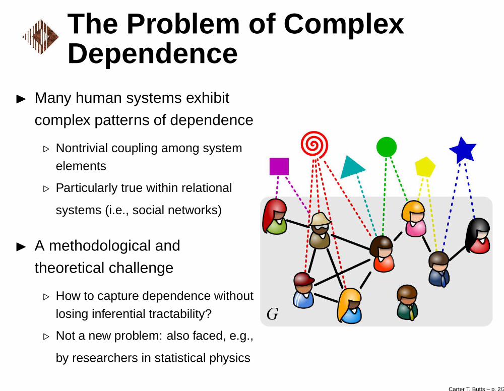
◮ Many human systems exhibit
complex patterns of dependence
⊲ Nontrivial coupling among systemelements
⊲ Particularly true within relational
systems (i.e., social networks)
◮ A methodological and
theoretical challenge
⊲ How to capture dependence withoutlosing inferential tractability?
⊲ Not a new problem: also faced, e.g.,
by researchers in statistical physics
Carter T. Butts – p. 2/20
Challenge: Modeling Realitywithout Sacrificing Data
◮ How do we work with models which have non-trivial dependence?
◮ Can compare behavior of dependent-process models against stylized
facts, but this has limits....
⊲ Not all models lead to clean/simple conditional or marginal relationships⊲ Often impossible to disentangle nonlinearly interacting mechanisms on this basis⊲ Very data inefficient: throws away much of the information content⊲ Often need (very) large data sets to get sufficient power (which may not exist)
⋄ Collection of massive data sets often prohibitively costly⋄ Many systems of interest are size-limited; studying only large systems leads to sampling
bias
◮ Ideally, would like a framework which allows principled
inference/model comparison without sacrificing (much) data
Carter T. Butts – p. 3/20

Our Focus: Stochastic Models for Social(and Other) Networks
◮ General problem: need to model graphs with varying properties
◮ Many ad hoc approaches:
⊲ Conditional uniform graphs (Erdös and Rényi, 1960)⊲ Bernoulli/independent dyad models (Holland and Leinhardt, 1981)⊲ Biased nets (Rapoport, 1949a;b; 1950)⊲ Preferential attachment models (Simon, 1955; Barabási and Albert, 1999)⊲ Geometric random graphs (Hoff et al., 2002)
⊲ Agent-based/behavioral models (Carley (1991); Hummon and Fararo (1995))
◮ A more general scheme: discrete exponential family models (ERGs)
⊲ General, powerful, leverages existing statistical theory (e.g., Barndorff-Nielsen (1978);Brown (1986); Strauss (1986))
⊲ (Fairly) well-developed simulation, inferential methods (e.g., Snijders (2002);
Hunter and Handcock (2006))
◮ Today’s focus – model parameterization
Carter T. Butts – p. 4/20

Basic Notation
◮ Assume G = (V, E) to be the graph formed by edge set E on vertex set V
⊲ Here, we take |V | = N to be fixed, and assume elements of V to be uniquelyidentified
⊲ If E ⊆˘
{v, v′} : v, v′ ∈ V¯
, G is said to be undirected ; G is directed iffE ⊆
˘
(v, v′) : v, v′ ∈ V¯
⊲ {v, v} or (v, v) edges are known as loops; if G is defined per the above andcontains no loops, G is said to be simple
⋄ Note that multiple edges are already banned, unless E is allowed to be a multiset
◮ Other useful bits
⊲ E may be random, in which case G = (V, E) is a random graph
⊲ Adjacency matrix Y ∈ {0, 1}N×N (may also be random); for G random, willusually use notation y for adjacency matrix of realization g of G
⊲ y+ij is used to denote the matrix y with the i, j entry forced to 1; y−
ij is the same
matrix with the i, j entry forced to 0
Carter T. Butts – p. 5/20

Exponential Families forRandom Graphs
◮ For random graph G w/countable support G, pmf is given in ERG form by
Pr(G = g|θ) =exp
(
θTt(g)
)
∑
g′∈Gexp (θT t(g′))
IG(g) (1)
◮ θTt: linear predictor
⊲ t : G → Rm: vector of sufficient statistics
⊲ θ ∈ Rm: vector of parameters
⊲∑
g′∈Gexp
(
θTt(g′)
)
: normalizing factor (aka partition function, Z)
◮ Intuition: ERG places more/less weight on structures with certain features,as determined by t and θ
⊲ Model is complete for pmfs on G, few constraints on t
Carter T. Butts – p. 6/20

Inference with ERGs
◮ Important feature of ERGs isavailability of inferential theory
⊲ Need to discriminate amongcompeting theories
⊲ May need to assess quantitative
variation in effect strengths, etc.
◮ Basic logic
⊲ Derive ERG parameterization fromprior theory
⊲ Assess fit to observed data
⊲ Select model/interpret parameters
⊲ Update theory and/or seek low-orderapproximating models
⊲ Repeat as necessary
Carter T. Butts – p. 7/20

Parameterizing ERGs
◮ The ERG form is a way of representingdistributions on G, not a model in and ofitself!
◮ Critical task: derive model statistics fromprior theory
◮ Several approaches – here we introduce anew one....
Carter T. Butts – p. 8/20

A New Direction: PotentialGames
◮ Most prior parameterization work has used dependence hypotheses⊲ Define the conditions under which one relationship could affect another, and hope that this
is sufficiently reductive
⊲ Complete agnosticism regarding underlying mechanisms – could be social dynamics,
unobserved heterogeneity, or secret closet monsters
◮ A choice-theoretic alternative?⊲ In some cases, reasonable to posit actors with some control over edges (e.g., out-ties)⊲ Existing theory often suggests general form for utility
⊲ Reasonable behavioral models available (e.g., multinomial choice)
◮ The link between choice models and ERGs: potential games⊲ Increasingly wide use in economics, engineering
⊲ Equilibrium behavior provides an alternative way to parameterize ERGs
Carter T. Butts – p. 9/20

Potential Games and NetworkFormation Games
◮ (Exact) Potential games (Monderer and Shapley, 1996)
⊲ Let X by a strategy set, u a vector utility functions, and V a set of players. Then (V, X, u) is
said to be a potential game if ∃ ρ : X 7→ R such that, for all i ∈ V ,
ui
`
x′i, x−i
´
− ui (xi, x−i) = ρ`
x′i, x−i
´
− ρ (xi, x−i) for all x, x′ ∈ X.
◮ Consider a simple family of network formation games (Jackson, 2006) on Y:
⊲ Each i, j element of Y is controlled by a single player k ∈ V with finite utility uk; can chooseyij = 1 or yij = 0 when given an “updating opportunity”
⋄ We will here assume that i controls Yi·, but this is not necessary
⊲ Theorem: Let (i) (V,Y, u) in the above form a game with potential ρ; (ii) players choose
actions via a logistic choice rule; and (iii) updating opportunities arise sequentially such that
every (i, j) is selected with positive probability, and (i, j) is selected independently of the
current state of Y. Then Y forms a Markov chain with equilibrium distribution
Pr(Y = y) ∝ exp(ρ(y)), in the limit of updating opportunities.
◮ One can thus obtain an ERG as the long-run behavior of a strategic process, andparameterize in terms of the hypothetical underlying utility functions
Carter T. Butts – p. 10/20

Proof of Potential GameTheorem
Assume an updating opportunity arises for yij , and assume that player k has control of yij . By thelogistic choice assumption,
Pr“
Y = y+ij
˛
˛Ycij = yc
ij
”
=exp
“
uk
“
y+ij
””
exp“
uk
“
y+ij
””
+ exp“
uk
“
y−ij
”” (2)
=h
1 + exp“
uk
“
y−ij
”
− uk
“
y+ij
””i−1. (3)
Since u,Y form a potential game, ∃ ρ : ρ“
y+ij
”
− ρ“
y−ij
”
= uk
“
y+ij
”
− uk
“
y−ij
”
∀ k, (i, j),ycij .
Therefore, Pr“
Y = y+ij
˛
˛
˛
Ycij = yc
ij
”
=h
1 + exp“
ρ“
y−ij
”
− ρ“
y+ij
””i−1. Now assume that the
updating opportunities for Y occur sequentially such that (i, j) is selected independently of Y, withpositive probability for all (i, j). Given arbitrary starting point Y(0), denote the updated sequence ofmatrices by Y(0),Y(1), . . .. This sequence clearly forms an irreducible and aperiodic Markov chainon Y (so long as ρ is finite); it is known that this chain is a Gibbs sampler on Y with equilibrium
distribution Pr(Y = y) =exp(ρ(y))
P
y′∈Y exp(ρ(y′)), which is an ERG with potential ρ. By the ergodic
theorem, then Y(i) −−−−→i→∞
ERG(ρ(Y)). QED.
Carter T. Butts – p. 11/20

Some Potential GameProperties
◮ Game-theoretic properties
⊲ Local maxima of ρ correspond to Nash equilibria in pure strategies; globalmaxima of ρ correspond to stochastically stable Nash equilibria in pure strategies
⋄ At least one maximum must exist, since ρ is bounded above for any given θ
⊲ Fictitious play property; Nash equilibria compatible with best responses to mean
strategy profile for population (interpreted as a mixed strategy)
◮ Implications for simulation, model behavior
⊲ Multiplying θ by a constant α → ∞ will drive the system to its SSNE
⋄ Likewise, best response dynamics (equivalent to conditional stepwise ascent) always
leads to a NE
⊲ For degenerate models, “frozen” structures represent Nash equilibria in theassociated potential game
⋄ Suggests a social interpretation of degeneracy in at least some cases: either correctly
identifies robust social regimes, or points to incorrect preference structureCarter T. Butts – p. 12/20

Building Potentials:Independent Edge Effects
◮ General procedure
⊲ Identify utility for actor i
⊲ Determine difference in ui for singleedge change
⊲ Find ρ such that utility difference is equal
to utility difference for all ui
◮ Linear combinations of payoffs
⊲ If ui (y) =P
j u(j)i (y),
ρ (y) =P
j ρ(j)i (y)
◮ Edge payoffs (homogeneous)
⊲ ui (y) = θP
j yij
⊲ ui
“
y+ij
”
− ui
“
y−ij
”
= θ
⊲ ρ (y) = θP
i
P
j yij
⊲ Equivalence: p1/Bernoulli density effect
◮ Edge payoffs (inhomogeneous)
⊲ ui (y) = θi
P
j yij
⊲ ui
“
y+ij
”
− ui
“
y−ij
”
= θi
⊲ ρ (y) =P
i θi
P
j yij
⊲ Equivalence: p1 expansiveness effect
◮ Edge covariate payoffs
⊲ ui (y) = θP
j yijxij
⊲ ui
“
y+ij
”
− ui
“
y−ij
”
= θxij
⊲ ρ (y) = θP
i
P
j yijxij
⊲ Equivalence: Edgewise covariate effects
(netlogit)
Carter T. Butts – p. 13/20

Building Potentials:Dependent Edge Effects
◮ Reciprocity payoffs
⊲ ui (y) = θP
j yijyji
⊲ ui
“
y+ij
”
− ui
“
y−ij
”
= θyji
⊲ ρ (y) = θP
i
P
j<i yijyji
⊲ Equivalence: p1 reciprocity effect
◮ 3-Cycle payoffs
⊲ ui (y) = θP
j 6=i
P
k 6=i,j yijyjkyki
⊲ ui
“
y+ij
”
− ui
“
y−ij
”
= θP
k 6=i,j yjkyki
⊲ ρ (y) = θ3
P
i
P
j 6=i
P
k 6=i,j yijyjkyki
⊲ Equivalence: Cyclic triple effect
◮ Transitive completion payoffs
⊲ ui (y) =
θP
j 6=i
P
k 6=i,j
2
4
yijykiykj + yijyikyjk
+yijyikykj
3
5
⊲ ui
“
y+ij
”
− ui
“
y−ij
”
=
θP
k 6=i,j
ˆ
ykiykj + yikyjk + yikykj
˜
⊲ ρ (y) = θP
i
P
j 6=i
P
k 6=i,j yijyikykj
⊲ Equivalence: Transitive triple effect
Carter T. Butts – p. 14/20

Empirical Example: Advice-Seeking AmongManagers
◮ Sample empirical application fromKrackhardt (1987): self-reportedadvice-seeking among 21 managers in ahigh-tech firm
⊲ Additional covariates: friendship, authority
(reporting)
◮ Demonstration: selection of potentialbehavioral mechanisms via ERGs
⊲ Models parameterized using utility components⊲ Model parameters estimated using maximum
likelihood (Geyer-Thompson)
⊲ Model selection via AIC
Carter T. Butts – p. 15/20

Advice-Seeking ERG – ModelComparison
◮ First cut: models with independent dyads:
Deviance Model df AIC Rank
Edges 578.43 1 580.43 7
Edges+Sender 441.12 21 483.12 4
Edges+Covar 548.15 3 554.15 5
Edges+Recip 577.79 2 581.79 8
Edges+Sender+Covar 385.88 23 431.88 2
Edges+Sender+Recip 405.38 22 449.38 3
Edges+Covar+Recip 547.82 4 555.82 6
Edges+Sender+Covar+Recip 378.95 24 426.95 1
◮ Elaboration: models with triadic dependence:
Deviance Model df AIC Rank
Edges+Sender+Covar+Recip 378.95 24 426.95 4
Edges+Sender+Covar+Recip+CycTriple 361.61 25 411.61 2
Edges+Sender+Covar+Recip+TransTriple 368.81 25 418.81 3
Edges+Sender+Covar+Recip+CycTriple+TransTriple 358.73 26 41 0.73 1
◮ Verdict: data supplies evidence for heterogeneous edge formation preferences (w/covariates),with additional effects for reciprocated, cycle-completing, and transitive-completing edges.
Carter T. Butts – p. 16/20

Advice-Seeking ERG – AICSelected Model
Effect θ s.e. Pr(> |Z|) Effect θ s.e. Pr(> |Z|)
Edges −1.022 0.137 0.0000 ∗ ∗ ∗ Sender14 −1.513 0.231 0.0000 ∗ ∗ ∗
Sender2 −2.039 0.637 0.0014 ∗∗ Sender15 16.605 0.336 0.0000 ∗ ∗ ∗
Sender3 0.690 0.466 0.1382 Sender16 −1.472 0.232 0.0000 ∗ ∗ ∗
Sender4 −0.049 0.441 0.9112 Sender17 −2.548 0.197 0.0000 ∗ ∗ ∗
Sender5 0.355 0.495 0.4734 Sender18 1.383 0.214 0.0000 ∗ ∗ ∗
Sender6 −4.654 1.540 0.0025 ∗∗ Sender19 −0.601 0.190 0.0016 ∗∗
Sender7 −0.108 0.375 0.7726 Sender20 0.136 0.161 0.3986
Sender8 −0.449 0.479 0.3486 Sender21 0.105 0.210 0.6157
Sender9 0.393 0.496 0.4281 Reciprocity 0.885 0.081 0.0000 ∗ ∗ ∗
Sender10 0.023 0.555 0.9662 Edgecov (Reporting) 5.178 0.947 0.0000 ∗ ∗ ∗
Sender11 −2.864 0.721 0.0001 ∗ ∗ ∗ Edgecov (Friendship) 1.642 0.132 0.0000 ∗ ∗ ∗
Sender12 −2.736 0.331 0.0000 ∗ ∗ ∗ CycTriple −0.216 0.013 0.0000 ∗ ∗ ∗
Sender13 −0.986 0.194 0.0000 ∗ ∗ ∗ TransTriple 0.090 0.003 0.0000 ∗ ∗ ∗
Null Dev 582.24; Res Dev 358.73 on 394 df
◮ Some observations...
⊲ Arbitrary edges are costly for most actors⊲ Edges to friends and superiors are “cheaper” (or even positive payoff)⊲ Reciprocating edges, edges with transitive completion are cheaper...
⊲ ...but edges which create (in)cycles are more expensive; a sign of hierarchy?
Carter T. Butts – p. 17/20

Model Adequacy Check
0 1 2 3 4 5 6 7 8 9 10 12 14 16 18 20
0.0
0.1
0.2
0.3
0.4
in degree
prop
ortio
n of
nod
es
0 1 2 3 4 5 6 7 8 9 10 12 14 16 18 20
0.00
0.05
0.10
0.15
0.20
0.25
out degree
prop
ortio
n of
nod
es
003 012 102 021U 111D 030T 201 120U 210 300
0.00
0.05
0.10
0.15
triad census
prop
ortio
n of
tria
ds
1 2 3 4 5 6 7 NR
0.0
0.1
0.2
0.3
0.4
0.5
minimum geodesic distance
prop
ortio
n of
dya
ds
Goodness−of−fit diagnostics
Carter T. Butts – p. 18/20

Where Would One Go Next?
◮ Model refinement
⊲ Goodness-of-fit is not unreasonable, but some improvement is clearly possible
⊲ Could refine existing model (e.g., by adding covariates) or propose more
alternatives
◮ Replication on new cases
⊲ Given a smaller set of candidates, would replicate on new organizations
⊲ May lead to further refinement/reformulation
◮ Simplification
⊲ Given a model family that works well, can it be simplified w/out losing too much?
⊲ Seek the smallest model which captures essential properties of optimal model;
general behavior can then be characterized (hopefully)
Carter T. Butts – p. 19/20

Summary
◮ Models for non-trivial networks pose non-trivial problems
⊲ Many ways to describe dependence among elements
⊲ Once one leaves simple cases, not always clear where to begin
◮ Potential games for ERG parameterization
⊲ Allow us to derive random cross-sectional behavior from strategic interaction
⊲ Provide sufficient conditions for ERG parameters to be interpreted in terms ofpreferences
⊲ Allows for testing of competing behavioral models (assuming scope conditions
are met!)
◮ Approach seems promising, but many questions remain
⊲ Can we characterize utilities which lead to identifiable models?
⊲ How can we leverage other properties of potential games?
Carter T. Butts – p. 20/20

1 References
Barabasi, A.-L. and Albert, R. (1999). Emergence of scaling in
random networks. Science, 206:509–512.
Barndorff-Nielsen, O. (1978). Information and Exponential
Families in Statistical Theory. John Wiley and Sons, New
York.
Brown, L. D. (1986). Fundamentals of Statistical Exponential
Families, with Applications in Statistical Decision Theory. In-
stitute of Mathematical Statistics, Hayward, CA.
Carley, K. M. (1991). A theory of group stability. American
Sociological Review, 56(3):331–354.
Erdos, P. and Renyi, A. (1960). On the evolution of random
graphs. Public Mathematical Institute of Hungary Academy
of Sciences, 5:17–61.
Harary, F. (1953). On the notion of balance of a signed graph.
Michigan Mathematical Journal, 3:37–41.
Heider, F. (1958). The Psychology of Interpersonal Relations.
John Wiley and Sons, New York.
20-1

Hoff, P. D., Raftery, A. E., and Handcock, M. S. (2002). Latent
space approaches to social network analysis. Journal of the
American Statistical Association, 97(460):1090–1098.
Holland, P. W. and Leinhardt, S. (1981). An exponential fam-
ily of probability distributions for directed graphs (with dis-
cussion). Journal of the American Statistical Association,
76(373):33–50.
Hummon, N. P. and Fararo, T. J. (1995). Assessing hierarchy
and balance in dynamic network models. Journal of Mathe-
matical Sociology, 20:145–159.
Hunter, D. R. and Handcock, M. S. (2006). Inference in curved
exponential family models for networks. Journal of Compu-
tational and Graphical Statistics, 15:565–583.
Jackson, M. (2006). A survey of models of network formation:
Stability and efficiency. In Demange, G. and Wooders, M.,
editors, Group Formation Economics: Networks, Clubs, and
Coalitions. Cambridge University Press, Cambridge.
Krackhardt, D. (1987). Cognitive social structures. Social Net-
works, 9(2):109–134.
Monderer, D. and Shapley, L. S. (1996). Potential games.
Games and Economic Behavior, 14:124–143.
20-2

Rapoport, A. (1949a). Outline of a probabilistic approach to ani-
mal sociology I. Bulletin of Mathematical Biophysics, 11:183–
196.
Rapoport, A. (1949b). Outline of a probabilistic approach to
animal sociology II. Bulletin of Mathematical Biophysics,
11:273–281.
Rapoport, A. (1950). Outline of a probabilistic approach to ani-
mal sociology III. Bulletin of Mathematical Biophysics, 12:7–
17.
Simon, H. A. (1955). On a class of skew distribution functions.
Biometrika, 42:425–440.
Snijders, T. A. B. (2002). Markov Chain Monte Carlo estima-
tion of exponential random graph models. Journal of Social
Structure, 3(2).
Strauss, D. (1986). On a General Class of Models for Interac-
tion. SIAM Review, 28(4):513–527.
20-3