Embed Size (px)
Citation preview

HAL Id: hal-01004976https://hal.archives-ouvertes.fr/hal-01004976
Submitted on 21 Feb 2017
HAL is a multi-disciplinary open accessarchive for the deposit and dissemination of sci-entific research documents, whether they are pub-lished or not. The documents may come fromteaching and research institutions in France orabroad, or from public or private research centers.
L’archive ouverte pluridisciplinaire HAL, estdestinée au dépôt et à la diffusion de documentsscientifiques de niveau recherche, publiés ou non,émanant des établissements d’enseignement et derecherche français ou étrangers, des laboratoirespublics ou privés.
Distributed under a Creative Commons Attribution| 4.0 International License
Active and passive earth pressure coefficients by akinematical approach
Abdul-Hamid Soubra, B. Macuh
To cite this version:Abdul-Hamid Soubra, B. Macuh. Active and passive earth pressure coefficients by a kinematicalapproach. Proceedings of the ICE - Geotechnical Engineering, Thomas Telford, 2002, 155 (2), pp.119-131. 10.1680/geng.2002.155.2.119. hal-01004976
Active and passive earth pressure coefficients by a kinematicalapproach
A.-H. Soubra and B. Macuh
A simple method is proposed for calculating the active
and passive earth pressure coefficients in the general
case of an inclined wall and a sloping backfill. The
approach used is based on rotational log-spiral failure
mechanisms in the framework of the upper-bound
theorem of limit analysis. It is shown that the energy
balance equation of a rotational log-spiral mechanism is
equivalent to the moment equilibrium equation about
the centre of the log-spiral. Numerical optimisation of
the active and passive earth pressure coefficients is
performed automatically by a spreadsheet optimisation
tool. The implementation of the proposed method is
illustrated using an example. The predictions by the
present method are compared with those given by other
authors.
NOTATION
c cohesion
dl elementary length along the slip surface BC_DD rate of energy dissipation
f1, f2, . . . , f8 intermediate non-dimensional functions
Kª, Kq, Kc earth pressure coefficients due to soil weight,
vertical surcharge loading and cohesion
Kaª, Kaq, Kac active earth pressure coefficients
Kpª, Kpq, Kpc passive earth pressure coefficients
Kaq0, Kpq0 active and passive earth pressure coefficients
due to a surcharge loading normal to the
ground surface
l=r0 and L=r0 intermediate non-dimensional functions
l wall length
L length of AB
Pa, Pp active and passive forces respectively
Pad adhesive force
q vertical surcharge loading
q0 surcharge loading normal to the ground
surface
r0, r1 initial and final radius of the log-spiral slip
surface
V velocity at the velocity discontinuity
W weight of the soil mass ABC_WW rate of work of an external force
Æ inclination of the Rankine earth pressure
slope of the backfill
ª unit weight of the soil
friction angle at the soil–structure interface
Ł0, Ł1 angles defining the log-spiral slip surface
º angle between the soil–wall interface and the
vertical direction
inclination of the Rankine slip surface with
the horizontal direction
normal stress acting on the slip surface
tangential stress acting on the slip surface
angle of internal friction of the soil
angular velocity of failure mechanism
1. INTRODUCTION
The problem of active and passive earth pressures acting
against rigid retaining structures has been extensively studied
in the literature since Coulomb.1
Most of the existing methods
are based on either the limit equilibrium method, the slip line
method or the limit analysis method.
Recently, a variational analysis has been applied to the passive
earth pressure problem by Soubra et al.2
Their approach is
based on a limit equilibrium method, and the solution provides
a log-spiral failure surface. For their failure wedge, the moment
equilibrium equation can be used for the calculation of the
passive earth pressures without specifying the normal stress
distribution along the log-spiral slip surface. It should be
emphasised that their method, employed in this paper, can be
categorised also as an upper-bound in the framework of limit
analysis where a rotational rigid body movement is considered.
This variational limit equilibrium method may be easily
extended to the active earth pressure problem, and the same
conclusions remain valid in this case:
(a) A log-spiral failure surface may be obtained from a
variational maximisation procedure.
(b) The moment equilibrium equation, which is equivalent to
the energy balance equation in the framework of the
upper-bound method of limit analysis, may be used for
computation of the active earth pressures.
The aim of this paper is to show that the upper-bound method
in limit analysis for a rotational log-spiral failure mechanism
gives rapid and good predictions for both active and passive
earth pressures. It is also demonstrated that the present method
can be easily implemented on a PC by defining spreadsheet

functions and by using a powerful spreadsheet optimisation
tool. The analysis is made in the general case of an inclined
wall and a sloping backfill, and considers a frictional and
cohesive (c, ) soil. A uniform surcharge is assumed to act
on the ground surface. Active and passive earth pressure
coefficients due to soil weight, cohesion and surcharge loading
are presented for various governing parameters and compared
with those given by other authors.
2. FAILURE MECHANISMS AND GOVERNING
EQUATIONS
The variational analysis details and the equivalence between
the variational limit equilibrium method and the upper-bound
method in limit analysis for a rotational log-spiral failure
mechanism are given elsewhere.2
However, for clarity, only the
upper-bound technique (that is, the kinematical approach) of
limit analysis is briefly described here.
Two rotational log-spiral failure mechanisms are considered in
the present analysis, one for the active state M1 (Fig. 1(a)) and
the other for the passive state M2 (Fig. 1(b)). For both M1 and
M2 mechanisms, the region ABC rotates as a rigid body about
the as yet undefined centre of rotation O relative to the
material below the logarithmic failure surface BC. Thus the
surface BC is a surface of velocity discontinuity. These failure
mechanisms can be specified completely by two variables
Ł0 and Ł1. It should be emphasised that the earth pressure
coefficient due to soil weight, Kª, is calculated with the
assumption of a cohesionless soil with no surcharge loading.
The computation of the coefficients Kq and Kc due to
surcharge loading and cohesion is based on the assumption of
a weightless soil with c ¼ 0 for Kq and q ¼ 0 for Kc. The
formulation for the coefficients of earth pressure due to soil
weight, surcharge and cohesion follows.
2.1. Rate of work of external forces
As shown in Fig. 1, the external forces acting on the soil
mass in motion consist of the self-weight of the soil, W, the
active or passive earth force (Pa or Pp), the adhesive force,
Pad(¼ cl tan = tan), and the surcharge, qL, acting on the
ground surface. The rate of work for the different external
forces can be calculated as follows.
2.1.1. Rate of work of the soil weight. A direct integration of
the rate of work of the soil weight in the region ABC is very
complicated. An easier alternative is first to find the rate of
work _WWOBC, _WWOAB and _WWOAC due to soil weight in the regions
OBC, OAB and OAC respectively. The rate of work for the
Ω
0
A
C
Br0
r1
Pad
Pa
r
l
L
θ1
θ0
λ > 0
β > 0
τσ
δ
φ
θ
q
r = r0·e–(θ – θ0)tan φ
(a)
W
Fig. 1. Log-spiral failure mechanisms: (a) M1 for active; (b) M2 for passive earth pressure analyses

region ABC is then found by simple algebraic summation,_WWOBC _WWOAB _WWOAC. The steps of computation of the rate of
work due to self-weight of the soil are essentially the same as
those of an inclined slope considered by Chen.3
It is found that
the rate of work due to the soil weight in the region ABC is
_WWsoil ¼ ªr30( f1 f2 f3)1
where f1, f2 and f3 are non-dimensional functions, which are
given in Appendix 1.
2.1.2. Rate of work of the active or passive force and the
adhesive force. The rate of work of the active or passive force
(Pa or Pp) and the adhesive force, Pad, can be expressed as
follows:
_WW(Pa or P p),Pad¼ Pa,p r0 f4 þ cr2
0 f52
where f4 and f5 are non-dimensional functions, which are
given in Appendix 1. It should be mentioned that the active or
passive force is assumed to act at the lower third of the wall
length for the calculation of the coefficients Kaª and Kpª.
However, the computation of Kac, Kpc, Kaq and Kpq is based on
the assumption that the point of application of the active or
passive force is applied at the middle of the wall length. These
hypotheses are in conformity with the classical earth pressure
distributions, and allow direct comparison with existing
solutions.
2.1.3. Rate of work of the surcharge loading. The rate of work
of the surcharge loading q can be expressed as follows:
_WWq ¼ qr20 f63
where f6 is a non-dimensional function, which is given in
Appendix 1.
The total rate of work of the external forces is the summation
of these three contributions—that is, equations (1), (2) and (3):
X[ _WW ]ext ¼ _WWsoil þ _WW(Pa or P p),Pad
þ _WWq4
2.2. Rate of energy dissipation
Since no general plastic deformation of the soil is permitted
to occur, the energy is dissipated solely at the velocity
discontinuity surface BC between the material at rest and the
material in motion. The rate of energy dissipation per unit area
of a velocity discontinuity can be expressed as3
Ω
0
A
C
B
r0
r1
Pad
Pp
r
l W
L
θ1
θ0
λ > 0
β > 0τ
σ
δ
φ
θ
q
r = r0·e(θ – θ0)tan φ
(b)
Fig. 1. (continued )

_DD ¼ cV cos5
where V is the velocity that makes an angle with the
velocity discontinuity. The total rate of energy dissipation
along BC can be expressed as follows:
_DDBC ¼ cr20 f76
where f7 is a non-dimensional function, which is given in
Appendix 1.
2.3. Energy balance equation
By equating the total rate of work of external forces (equation
(4)) to the total rate of energy dissipation (equation (6)), we
have
ªr30( f1 f2 f3)þ Pa,p r0 f4 þ cr2
0 f5 þ qr20 f6 ¼ cr2
0 f77
The energy balance equation of the rotational log-spiral
mechanism (i.e. equation (7)) is identical to the moment
equilibrium equation about the centre of the log-spiral. It
should be emphasised that the log-spiral function has a
particular property, that the resultant of the forces ( dl ) and
(tan dl ) passes through the pole of the spiral. Hence the
moment equilibrium equation of the soil mass in motion about
the centre of the log-spiral is independent of the normal stress
distribution along the slip surface. Based on equation (7), the
active and passive forces can be expressed respectively as
follows:
Pa ¼ Kaªªl2
2þ Kaqql Kaccl8
Pp ¼ Kpªªl2
2þ Kpqqlþ Kpccl9
where Kaª, Kpª, Kaq, Kpq, Kac and Kpc are the earth pressure
coefficients. The coefficients Kª, Kq and Kc represent
respectively the effect of soil weight, vertical surcharge loading
and cohesion, and the subscripts a and p represent the active
and passive cases respectively. These coefficients are given as
follows, using the lower sign for the passive case:
Kaª ¼ K pª ¼2
l
r0
2 ( f1 f2 f3)
f 410
Kaq ¼ K pq ¼1l
r0
f6
f 411
Kac,pc ¼ 1l
r0
f 7 f 5
f 412
For a surcharge loading q0 normal to the ground surface, the
active and passive earth pressure coefficients, Kaq0 and Kpq0,
are given as follows:
Kaq0,pq0 ¼ 1l
r0
f8
f413
where f8 is a non-dimensional function, which is given in
Appendix 1.
3. NUMERICAL RESULTS
The most critical earth pressure coefficients can be obtained by
numerical maximisation of the coefficients Kaª, Kaq and Kaq0
and minimisation of the coefficients Kac, Kpª, Kpq, Kpq0
and Kpc. These optimisations are made with regard to the
parameters Ł0 and Ł1. The procedure can be performed using
the optimisation tool available in most spreadsheet software
packages. In this paper the Solver optimisation tool of
Microsoft Excel has been used. Two computer programs have
been developed using Visual Basic for Applications (VBA) to
define the active and passive earth pressure coefficients as
functions of the two angular parameters Ł0 and Ł1 defined in
Fig. 1.
In the following sections, the passive and active earth pressure
coefficients obtained from the present analysis are presented
and compared with those given by other authors. Then a
demonstration of the implementation of earth pressure
coefficients as user-defined functions in Microsoft Excel Visual
Basic is presented. An illustrative example shows the easy use
of spreadsheets in optimisation problems. The paper ends with
the presentation of two design tables giving some values of the
active and passive earth pressure coefficients for practical use
in geotechnical engineering.
3.1. Passive earth pressure coefficients
There are a great many solutions for the passive earth pressure
problem in the literature based on
(a) the limit equilibrium method4–15
(b) the slip line method16–20
(c) limit analysis theory.2, 21–28
The tendency today in practice is to use the values given by
Kerisel and Absi.29
3.1.1. Comparison with Rankine solution. For the general case
of an inclined wall and a sloping backfill (º= 6¼ 0, = 6¼ 0),
the Rankine passive earth pressure is inclined at an angle Æwith the normal to the wall irrespective of the angle of friction
at the soil–wall interface,30
where
tanÆ ¼ sin(ø þ 2º)sin
1þ sin cos(ø þ 2º)14

and
sinø ¼sin
sin15
The inclination of the slip surface with the horizontal direction
is given as follows:
¼ ø þ
2þ
4
216
and the coefficient Kpª is given by
Kpª ¼cos(º )sinø
cosÆ sin(ø )[1þ sin cos(ø þ 2º)]17
In order to validate the results of the present analysis, one
considers a soil–wall friction angle equal to the Æ value
given by equation (14). The numerical solutions obtained by
the computer program have shown that, in these cases, the
present results are similar to the exact solutions given by
Rankine (that is, equations (16) and (17)); the log-spiral slip
surface degenerates to a planar surface with radii approaching
infinity.
It should be emphasised that the results obtained from the
computer program indicate that the coefficient Kpc is related to
the coefficient Kpq0 by the following relationship (cf. Caquot’s
theorem of corresponding states31
):
Kpc ¼Kpq0
1
costan
18
Also, it should be mentioned that the critical angular
parameters Ł0 and Ł1 obtained from the minimisation of both
Kpq0 and Kpc give exactly the same critical geometry.
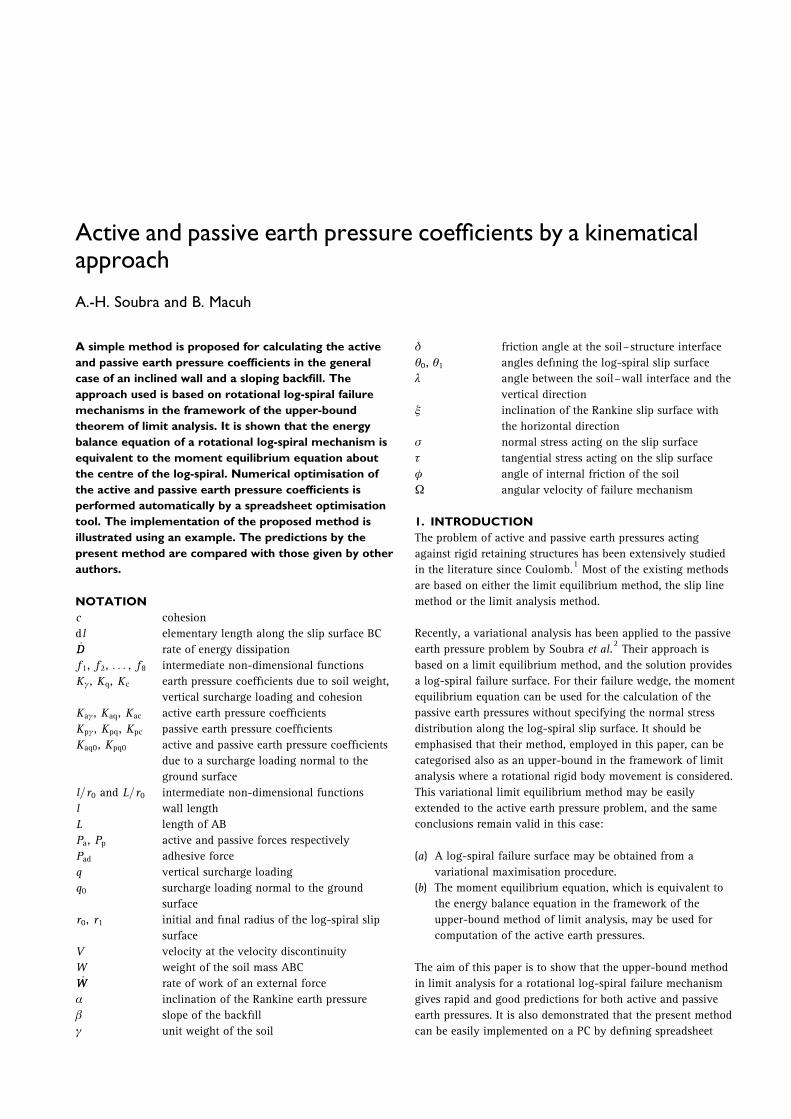
3.1.2. Comparison with Kerisel and Absi. Figures 2 and 3
show the comparison of the present solutions of Kpª and Kpq
with those of Kerisel and Absi29
for the case of a vertical wall
and an inclined backfill, and for the case of an inclined wall
and a horizontal backfill respectively, when ¼ 408.
For the Kpª coefficient, the present results are greater than
those of Kerisel and Absi. However, the maximum difference
does not exceed 13%. For the Kpq coefficient, the present
solutions continue to be greater than those of Kerisel and Absi;
a maximum difference of 22% is obtained for the extreme case
when ¼ 408, = ¼ 1, = ¼ 0 and º ¼ 308.
To conclude, the present solutions of Kpª and Kpq are greater
than the ones given by Kerisel and Absi. However, for practical
configurations ( < 408, 1=3 < = < 2=3, = < 1=3 and
º ¼ 08), the maximum difference does not exceed 5% for Kpª
and 7% for Kpq.
3.1.3. Comparison with the existing upper-bound
solutions. Rigorous upper-bound solutions of the passive earth
pressure problem are proposed in the literature by Chen and
Rosenfarb23
and Soubra.27
Chen and Rosenfarb considered six
translational failure mechanisms and showed that the log-
sandwich mechanism gives the least (that is, the best) upper-
bound solutions. Recently, Soubra27
considered a translational
multiblock failure mechanism and improved significantly the
existing upper-bound solutions given by the log-sandwich
mechanism for the Kpª coefficient, since he obtained smaller
upper bounds. The improvement (that is, the reduction relative
to Chen and Rosenfarb’s upper-bound solution) attains 21%
when ¼ 458, = ¼ 1, = ¼ 1 and º ¼ 158.
The results of Kpª and Kpq given by the present rotational
failure mechanism and those given by Soubra27
using a
translational failure mechanism are presented in Fig. 4 for the
general case of an inclined wall and a sloping backfill when
¼ 458 and = ¼ 1.
For the Kpª coefficient, the present upper-bound solutions
are smaller (that is, better) than those of Soubra.27
The
improvement (that is, the reduction relative to Soubra’s upper-
bound solution) is 27% when ¼ 458, = ¼ 1, = ¼ 1 and
º ¼ 158. For the Kpq coefficient, it should be mentioned that
the values obtained by Soubra27
are identical to those given by
Kerisel and Absi29
and correspond to the exact solutions for a
100
90
80
70
60
50
40
30
20
10
0
Kpγ
50
40
30
20
10
5
15
25
35
45
0
Kpq
Present solutionKérisel and Absi
–40 –30 –20 –10 0 10 20 30 40β
δ/φ = 1
δ/φ = 1/2
δ/φ = 0
Present solutionKérisel and Absi
δ/φ = 1
δ/φ = 1/2
δ/φ = 0
Fig. 2. Comparison of present Kpª and Kpq coefficientswith those of Kerisel and Absi
29(for vertical wall and
inclined backfill)
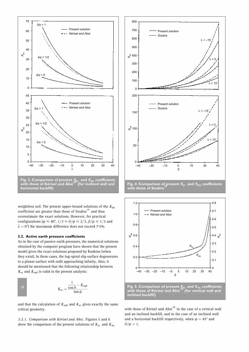
weightless soil. The present upper-bound solutions of the Kpq
coefficient are greater than those of Soubra27
and thus
overestimate the exact solutions. However, for practical
configurations ( < 408, 1=3 < = < 2=3, = < 1=3 and
º ¼ 08) the maximum difference does not exceed 7·5%.
3.2. Active earth pressure coefficients
As in the case of passive earth pressures, the numerical solutions
obtained by the computer program have shown that the present
model gives the exact solutions proposed by Rankine (when
they exist). In these cases, the log-spiral slip surface degenerates
to a planar surface with radii approaching infinity. Also, it
should be mentioned that the following relationship between
Kac and Kaq0 is valid in the present analysis:
Kac ¼1
cos Kaq0
tan19
and that the calculation of Kaq0 and Kac gives exactly the same
critical geometry.
3.2.1. Comparison with Kerisel and Absi. Figures 5 and 6
show the comparison of the present solutions of Kaª and Kaq
with those of Kerisel and Absi29
in the case of a vertical wall
and an inclined backfill, and in the case of an inclined wall
and a horizontal backfill respectively, when ¼ 458 and
= ¼ 1.
70
60
50
40
30
20
10
0
Kpγ
40
30
20
10
5
15
25
35
45
0
Kpq
Present solutionKérisel and Absi
–40 –30 –20 –10 0 10 20 30 40λ
δ/φ = 1
δ/φ = 1/2
δ/φ = 0
Present solutionKérisel and Absiδ/φ = 1
δ/φ = 1/2
δ/φ = 0
Fig. 3. Comparison of present Kpª and Kpq coefficientswith those of Kerisel and Absi
29(for inclined wall and
horizontal backfill)
100
200
300
500
400
600
700
800
0
Kpγ
200
150
50
100
0
Kpq
–45 –30 –15 0 15 30 45β
Present solutionSoubra
λ = –15˚
λ = 15˚
λ = 0
Present solutionSoubra
λ = –15˚
λ = 15˚
λ = 0
Fig. 4. Comparison of present Kpª and Kpq coefficientswith those of Soubra
27
Kaγ
Kaγ
0
0·2
0
0·1
0·2
0·3
0·4
0·5
0·6
0·7
0·8
0·4
0·6
0·8
1·0
1·2
Kaq
Kaq
–45 –35 –25 –15 –5 5 15 25 35 45β
Present solutionKérisel and Absi
Fig. 5. Comparison of present Kaª and Kaq coefficientswith those of Kerisel and Absi
29(for vertical wall and
inclined backfill)

The present results are smaller than those of Kerisel and Absi.
For the Kaª coefficient, the maximum difference does not
exceed 3% when º < 158; however, for º ¼ 208 a significant
difference is observed. After careful examination of the values
proposed by Kerisel and Absi for similar configurations (see for
instance their values for = ¼ 0:66 or 0), it seems that their
Kaª value for ¼ 458, = ¼ 1, ¼ 08 and º ¼ 208 is not
correct. For the Kaq coefficient the underestimation does not
exceed 8%.
The preceding comparisons allow one to conclude that, for
practical configurations ( < 408, = < 1, = > 1=3 and
º ¼ 08), there is good agreement with the currently used results
of Kerisel and Absi for both Kaª and Kaq. The maximum
difference does not exceed 3%.
4. IMPLEMENTATION
OF USER-DEFINED
FUNCTIONS IN VISUAL
BASIC FOR
APPLICATIONS, AND
THE USE OF SOLVER
To implement the functions
defining the passive earth
pressure coefficients and to
run the Solver optimisation
tool of Microsoft Excel, one
has to follow the following
steps (for the active case, use
the appropriate equations
given in Appendix 1):
(a) Create the user-defined
functions shown in
Appendix 2. This is done
in Microsoft Excel 97 by
first clicking Tools/
Macro/Visual Basic Editor
and then clicking Insert/
Module and, in the module sheet, typing ‘Option explicit
. . .’, etc. The functions are simple and self-explanatory.
(b) As shown in Fig. 7, cells C5, C6, C7 and C8 are input data
that define the mechanical and geometrical parameters ,
, º and . Cells C12 and C13 contain values of angular
parameters of the log-spiral slip surface Ł0 and Ł1. Finally,
cell C19 contains the formula to compute the passive earth
pressure coefficient Kpª. Arbitrary values were initially
entered in cells C12 and C13 for Ł0 and Ł1, say 0·5 for Ł0
and 1·5 for Ł1.
(c) Invoke the Solver tool by clicking Tools/Solver. Fig. 8
shows the Solver dialog box. To calculate the Kpª
coefficient, set the C19 cell ‘equal to’ minimum, ‘by
changing’ cells C12 and C13, namely Ł0 and Ł1, ‘subject to’
the constraints that C13 > C12þ 0:0001 (Ł1 . Ł0),
C12 < 3:14 (Ł0 < ), C13 < 3:14 (Ł1 < ),
C13 > 0 (Ł1 > 0) and C19 > 0 (Kpª > 0).
If Solver reports a converged solution, one should accept the
solution and re-invoke Solver, until it reports it has ‘found
a solution’. It should be mentioned that the initial values of Ł0
and Ł1 may influence the ability of the Solver to find a
solution. This need for judicious choice of starting values of Ł0
and Ł1 is not a major inconvenience because different starting
values can be tried with ease using the proposed spreadsheet
approach. The appealing feature of the spreadsheet approach is
that once the spreadsheet is set up as shown in Fig. 7, running
other problems with different geometry and soil properties
merely requires changing the input data (that is, , , and º).
4.1. Illustrative example
Consider the following characteristics: ¼ 408, = ¼ 2=3,
= ¼ 0 and º ¼ 08. Initial values of Ł0 and Ł1 are arbitrarily
chosen, say 0·5 for Ł0 and 1·5 for Ł1. Fig. 7 shows the critical
coefficient Kpª ¼ 12:59 and the corresponding critical slip
surface.
Kaγ
Kaγ
0
0·2
0·3
0·1
0
0·1
0·2
0·3
0·4
0·50·4
Kaq
Kaq
–20 –10 0 2010λ
Present solutionKérisel and Absi
Fig. 6. Comparison of present Kaª and Kaq coefficientswith those of Kerisel and Absi
29(for inclined wall and
horizontal backfill)
Fig. 7. Calculation of passive earth pressure coefficient Kpª using spreadsheet

5. DESIGN TABLES
Tables 1 and 2 present the coefficients Kpª, Kpq, Kpc, Kaª, Kaq
and Kac obtained from the computer programs for practical use
in geotechnical engineering. These values are given for ranging from 208 to 408, for five values of =, for º ¼ 08 and
for four values of =. For practical configurations, the passive
(or active) earth pressure coefficients are given for negative (or
positive) values.
6. CONCLUSIONS
A simple method using spreadsheet software has been proposed
for computing the active and passive earth pressure
coefficients. The method is based on the upper-bound theorem
of limit analysis. The failure mechanism is of the rotational
type. It is bounded by a log-spiral slip surface. The energy
balance equation is shown to be equivalent to the moment
equilibrium equation about the centre of the log-spiral. The
present approach gives rigorous solutions for the active and
passive earth pressures in the framework of the kinematical
approach of limit analysis.
Numerical optimisation is performed automatically by a
spreadsheet optimisation tool. The implementation of the
proposed method has been illustrated using an example. Once
the spreadsheet has been set up, the same template can be used
for analysing other problems merely by changing the input
data. The advantage of this method is its simplicity in use.
Comparison with the currently used solutions of Kerisel and
Absi29
leads to the following conclusions:
(a) For the passive case, the present solutions of Kpª and Kpq
are greater than those given by Kerisel and Absi.29
However, for practical configurations ( < 408, 1=3 < =< 2=3, = < 1=3 and º ¼ 08), the maximum difference
does not exceed 5% for Kpª and 7% for Kpq.
(b) For the active case, the present solutions of Kaª and Kaq
allow one to conclude that for practical configurations
( < 408, = < 1, = > 1=3 and º ¼ 08), there is good
agreement with the currently used results of Kerisel and
Absi. The maximum difference does not exceed 3%.
On the other hand, the present analysis improves the best
upper-bound solutions given in the literature by Soubra27
for
the Kpª coefficient. The improvement (that is, the reduction
relative to Soubra’s upper-bound solution) is 27% when
¼ 458, = ¼ 1, = ¼ 1 and º ¼ 158. For the Kpq
coefficient, the present analysis overestimates the upper-bound
solutions given by Soubra. However, for practical
configurations ( < 408, 1=3 < = < 2=3, = < 1=3 and
º ¼ 08) the maximum difference does not exceed 7·5%.
Numerical results of the active and passive earth pressure
coefficients are given in a tabular form for practical use. The
proposed method, being simple and rigorous, may be an
attractive alternative to other existing solutions, and can be
easily extended to other stability problems in geotechnical
engineering.
APPENDIX 1
The non-dimensional functions f1, f2, . . . , f8 are given as
follows, using the lower sign for the passive case:
f1 ¼
e 3(Ł1Ł0)tan (3 tan sin Ł1 cos Ł1) 3 tan sin Ł0 þ cosŁ0
3(9 tan 2þ 1)
264
37520
f2 ¼ 1
6
L
r02 sin Ł0 2
l
r0sin ºþ L
r0cos
cos (Ł1 ) e(Ł1Ł0) tan
21
f3 ¼ 1
6
l
r0sin Ł0 ºð Þ 2 sin Ł0
l
r0sin º
22
f4 ¼
cos( º) cos Ł0 1
3
l
r0cos º
sin ( º) sin Ł0 1
3
l
r0sin º
for Kº
cos( º) cos Ł0 1
2
l
r0cos º
sin( º) sin Ł0 1
2
l
r0sin º
for Kq, Kq0 and Kc
8>>>>>>>>>>>>>><>>>>>>>>>>>>>>:
23
f5 ¼l
r0
tan
tan sin(º Ł0)24
f6 ¼ L
r0sin Ł0 þ
l
r0sin º 1
2
L
r0cos
25
f7 ¼ 1
2 tan(e2(Ł1Ł0)tan 1)26
Fig. 8. Solver dialog box

K
pª
Kpq
Kpc
=
=
=
=
01=3
1=2
2=3
10
1=3
1=2
2=3
10
1=3
1=2
2=3
1
20
02·0
42·3
92·5
72·7
53·1
32·0
42·3
82·5
42·7
03·0
02·8
63·7
64·1
84·5
95·3
1
1=3
1·7
11·9
42·0
72·2
12·4
91·7
21·9
62·0
92·2
12·4
62·4
33·2
13·5
93·9
44·5
7
1=2
1·5
51·7
31·8
31·9
42·1
61·5
81·7
51·8
51·9
62·1
82·2
42·9
63·3
13·6
44·2
3
2=3
1·3
91·5
11·5
81·6
61·8
31·4
31·5
51·6
21·7
01·8
72·0
72·7
23·0
53·3
63·9
125
02·4
63·0
73·4
13·7
64·5
42·4
63·0
43·3
43·6
54·2
43·1
44·3
64·9
85·5
86·7
4
1=3
1·9
42·3
22·5
42·7
73·3
01·9
62·3
42·5
62·7
93·2
62·5
13·5
04·0
24·5
25·4
7
1=2
1·7
11·9
72·1
32·3
12·7
21·7
52·0
22·1
82·3
72·7
52·2
63·1
33·5
94·0
54·9
1
2=3
1·4
71·6
51·7
51·8
82·1
71·5
41·7
21·8
31·9
62·2
62·0
32·7
83·2
03·6
24·3
930
03·0
04·0
34·6
55·3
46·9
33·0
03·9
84·5
35·1
06·2
83·4
65·1
46·0
56·9
98·8
8
1=3
2·2
02·7
73·1
43·5
64·5
42·2
42·8
23·1
83·5
74·4
42·5
93·8
44·5
45·2
66·7
1
1=2
1·8
72·2
52·5
02·8
03·5
21·9
32·3
32·5
92·8
93·5
82·2
63·2
93·9
14·5
45·8
0
2=3
1·5
51·7
91·9
42·1
32·6
21·6
51·9
02·0
72·2
72·7
61·9
72·8
33·3
53·8
94·9
935
03·6
95·4
46·5
97·9
511·3
03·6
95·3
56·3
47·4
29·8
23·8
46·1
87·5
59·0
512·2
8
1=3
2·5
03·3
53·9
54·6
76·5
32·5
53·4
34·0
24·7
06·3
12·6
64·2
15·1
86·2
38·5
0
1=2
2·0
32·5
72·9
63·4
44·7
02·1
32·7
03·1
03·5
94·7
92·2
33·4
64·2
65·1
37·0
2
2=3
1·6
21·9
32·1
52·4
33·2
21·7
62·1
02·3
42·6
53·4
71·8
92·8
53·4
84·2
05·7
540
04·6
07·6
29·8
112·6
020·0
14·6
07·4
29·2
711·4
016·4
34·2
97·6
29·7
712·2
618·0
2
1=3
2·8
34·1
05·0
96·3
59·9
32·9
14·2
25·2
06·3
99·4
22·7
04·6
66·0
07·5
611·2
1
1=2
2·2
02·9
53·5
34·3
06·5
52·3
43·1
43·7
54·5
56·6
92·1
93·6
24·6
65·8
88·7
5
2=3
1·6
72·0
82·3
82·7
94·0
61·8
72·3
22·6
63·1
24·4
71·7
82·8
43·6
04·5
46·7
7
Tab
le1.P
ass
ive
eart
hp
ress
ure
co
effi
cie
nts
Kpª,
Kp
qan
dK
pc

K
aªK
aqK
ac
=
=
=
=
01=3
1=2
2=3
10
1=3
1=2
2=3
10
1=3
1=2
2=3
1
20
00·4
90
0·4
59
0·4
49
0·4
42
0·4
36
0·4
90
0·4
60
0·4
50
0·4
44
0·4
41
1·4
00
1·5
03
1·5
53
1·6
03
1·7
12
1=3
0·5
37
0·5
07
0·4
97
0·4
90
0·4
85
0·5
41
0·5
11
0·5
01
0·4
94
0·4
91
1·5
11
1·6
09
1·6
58
1·7
08
1·8
19
1=2
0·5
69
0·5
41
0·5
31
0·5
25
0·5
20
0·5
78
0·5
49
0·5
39
0·5
33
0·5
30
1·5
64
1·6
60
1·7
07
1·7
57
1·8
69
2=3
0·6
11
0·5
86
0·5
77
0·5
72
0·5
70
0·6
28
0·6
02
0·5
93
0·5
88
0·5
86
1·6
16
1·7
08
1·7
55
1·8
05
1·9
17
25
00·4
06
0·3
78
0·3
69
0·3
64
0·3
63
0·4
06
0·3
78
0·3
70
0·3
66
0·3
68
1·2
74
1·3
57
1·4
02
1·4
53
1·5
77
1=3
0·4
51
0·4
23
0·4
15
0·4
10
0·4
10
0·4
56
0·4
27
0·4
19
0·4
15
0·4
17
1·3
87
1·4
63
1·5
07
1·5
58
1·6
85
1=2
0·4
82
0·4
55
0·4
47
0·4
43
0·4
44
0·4
93
0·4
66
0·4
58
0·4
54
0·4
56
1·4
38
1·5
12
1·5
55
1·6
06
1·7
34
2=3
0·5
23
0·4
99
0·4
92
0·4
89
0·4
93
0·5
46
0·5
21
0·5
14
0·5
11
0·5
15
1·4
87
1·5
58
1·6
01
1·6
51
1·7
79
30
00·3
33
0·3
09
0·3
03
0·3
00
0·3
04
0·3
33
0·3
10
0·3
04
0·3
02
0·3
09
1·1
55
1·2
23
1·2
67
1·3
20
1·4
66
1=3
0·3
74
0·3
50
0·3
43
0·3
41
0·3
47
0·3
79
0·3
55
0·3
49
0·3
47
0·3
54
1·2
62
1·3
24
1·3
67
1·4
21
1·5
71
1=2
0·4
02
0·3
79
0·3
73
0·3
71
0·3
79
0·4
16
0·3
92
0·3
86
0·3
84
0·3
93
1·3
10
1·3
68
1·4
11
1·4
64
1·6
15
2=3
0·4
41
0·4
20
0·4
15
0·4
14
0·4
25
0·4
69
0·4
46
0·4
42
0·4
41
0·4
53
1·3
53
1·4
08
1·4
50
1·5
03
1·6
56
35
00·2
71
0·2
51
0·2
47
0·2
47
0·2
56
0·2
71
0·2
52
0·2
48
0·2
48
0·2
60
1·0
41
1·0
99
1·1
43
1·2
01
1·3
73
1=3
0·3
06
0·2
86
0·2
82
0·2
82
0·2
93
0·3
12
0·2
92
0·2
88
0·2
88
0·3
02
1·1
40
1·1
91
1·2
35
1·2
93
1·4
71
1=2
0·3
30
0·3
11
0·3
08
0·3
08
0·3
22
0·3
46
0·3
26
0·3
23
0·3
23
0·3
39
1·1
80
1·2
29
1·2
72
1·3
31
1·5
11
2=3
0·3
65
0·3
47
0·3
45
0·3
47
0·3
64
0·3
98
0·3
78
0·3
76
0·3
78
0·3
97
1·2
16
1·2
62
1·3
04
1·3
63
1·5
44
40
00·2
17
0·2
02
0·2
00
0·2
02
0·2
15
0·2
17
0·2
03
0·2
01
0·2
03
0·2
19
0·9
33
0·9
83
1·0
29
1·0
92
1·2
95
1=3
0·2
46
0·2
31
0·2
29
0·2
31
0·2
48
0·2
53
0·2
37
0·2
35
0·2
38
0·2
56
1·0
19
1·0
64
1·1
09
1·1
74
1·3
85
1=2
0·2
67
0·2
52
0·2
50
0·2
53
0·2
72
0·2
84
0·2
68
0·2
66
0·2
69
0·2
91
1·0
52
1·0
95
1·1
40
1·2
04
1·4
18
2=3
0·2
96
0·2
82
0·2
82
0·2
86
0·3
10
0·3
32
0·3
16
0·3
16
0·3
20
0·3
47
1·0
79
1·1
20
1·1
64
1·2
29
1·4
45
Tab
le2.A
cti
ve
eart
hp
ress
ure
co
effi
cie
nts
Kaª,
Kaq
an
dK
ac

f8 ¼L
r0sin( Ł0)þ
l
r0sin(º ) 1
2
L
r0
27
where
L
r0¼
e 3(Ł1Ł0)tan (sinŁ1 cosŁ1 tan º) sin Ł0 þ cos Ł0 tan º
sin tan ºþ cos 28
l
r0¼ e(Ł1Ł0)tan cos(Ł1 )þ cos(Ł0 )
cos( º)29
APPENDIX 2
The user-defined functions for passive earth pressure
coefficients coded in Microsoft Excel Visual Basic are as
follows:
' Program for evaluation of Kpgama, Kpc and Kpq for rotational' mechanism using log-spiral slip surfaceOption Explicit ' All variables must be declared' Definition of the global constantsPublic Const Pi = 3.141592654' VariablesPublic Phi As Double ' internal friction angle of the soilPublic Delta As Double ' angle of friction between soil and wallPublic Lambda As Double ' inclination of the wallPublic Beta As Double ' inclination of the backfillPublic Sl_r0 As Double ' l/r0Public CL_r0 As Double ' L/r0' Unknown variablesPublic Theta0 As Double ' first unknown angle (in radians)Public Theta1 As Double ' second unknown angle (in radians)' Defining the initial valuesSub Define()Phi = Cells(5, 3).Value * Pi / 180# ' Values from the cellsDelta = Cells(6, 3).Value * Pi / 180#Lambda = Cells(7, 3).Value * Pi / 180#Beta = Cells(8, 3).Value * Pi / 180#Theta0 = Cells(12, 3).ValueTheta1 = Cells(13, 3).ValueSl_r0 = (-Exp((Theta1 - Theta0) * Tan(Phi)) * Cos(Theta1 - Beta) _+ Cos(Theta0 - Beta)) / Cos(Beta - Lambda)CL_r0 = (Exp((Theta1 - Theta0) * Tan(Phi)) _* (Sin(Theta1) - Cos(Theta1) * Tan(Lambda)) - _Sin(Theta0) + Cos(Theta0) * Tan(Lambda)) / _(Sin(Beta) * Tan(Lambda) + Cos(Beta))End Sub'***********************************************Function f_1() As DoubleDim C1#, C2#C1 = Exp(3# * (Theta1 - Theta0) * Tan(Phi))C2 = 3# * (9# * (Tan(Phi)) ^ 2 + 1)f_1 = -(C1 * (3# * Tan(Phi) * Sin(Theta1) - Cos(Theta1)) - _3# * Tan(Phi) * Sin(Theta0) + Cos(Theta0)) / C2End Function'***********************************************Function f_2() As DoubleDim C1#, C2#C1 = 2# * Sin(Theta0) - 2# * Sl_r0 * Sin(Lambda) + CL_r0 * Cos(Beta)C2 = CL_r0 * Cos(Theta1 - Beta) * Exp((Theta1 - Theta0) * Tan(Phi))f_2 = -(1# / 6#) * C1 * C2End Function'***********************************************Function f_3() As Doublef_3 = -(1# / 6#) * Sl_r0 * Sin(Theta0 - Lambda) * _(2# * Sin(Theta0) - Sl_r0 * Sin(Lambda))End Function'***********************************************Function f_4_Kpg() As DoubleDim C1#, C2#C1 = Cos(Delta - Lambda) * (Cos(Theta0) - Sl_r0 / 3# * Cos(Lambda))C2 = Sin(Delta - Lambda) * (Sin(Theta0) - Sl_r0 / 3# * Sin(Lambda))f_4_Kpg = C1 - C2End Function

REFERENCES
1. COULOMB C. A. Sur une application des regles de maximis
et minimis a quelques problemes de statique relatifs a
l’architecture. Acad. R. Sci. Mem. Math. Phys., 1773, 7,
343–382.
2. SOUBRA A.-H., KASTNER R. and BENMANSOUR A. Passive
earth pressures in the presence of hydraulic gradients.
Geotechnique, 1999, 49, No. 3, 319–330.
3. CHEN W. F. Limit Analysis and Soil Plasticity. Elsevier,
Amsterdam, 1975.
4. TERZAGHI K. Theoretical Soil Mechanics. Wiley, New York,
1943.
5. JANBU N. Earth pressure and bearing capacity calculations
by generalised procedure of slices. Proceedings of the
Fourth International Conference, International Society of
Soil Mechanics and Foundation Engineering, 1957, 2,
207–213.
6. ROWE P. W. Stress-dilatancy, earth pressures, and slopes.
Journal of the Soil Mechanics and Foundation Division,
ASCE, 1963, 89, No. SM3, 37–61.
7. LEE J. K. and MOORE P. J. Stability Analysis: Application to
Slopes, Rigid and Flexible Retaining Structures. Selected
Topics in Soil Mechanics. Butterworth, London, 1968.
8. PACKSHAW S. Earth Pressure and Earth Resistance: A
Century of Soil Mechanics. Institution of Civil Engineers,
London, 1969.
9. SHIELDS D. H. and TOLUNAY A. Z. Passive pressure
coefficients for sand by the Terzaghi and Peck method.
Canadian Geotechnical Journal, 1972, 9, No. 4, 501–503.
10. SHIELDS D. H. and TOLUNAY A. Z. Passive pressure
coefficients by method of slices. Journal of the
Geotechnical Engineering Division, Proceedings of the
ASCE, 1973, 99, No. SM12, 1043–1053.
11. SPENCER E. Forces on retaining walls using the method of
slices. Civil Engineering, 1975, 18–23.
12. RAHARDJO H. and FREDLUND D. G. General limit equilibrium
method for lateral earth forces. Canadian Geotechnical
Journal, 1984, 21, No. 1, 166–175.
13. BILZ P., FRANKE D. and PIETSCH C. Earth pressure of soils
with friction and cohesion. Proceedings of the Eleventh
International Conference on Soil Mechanics and Foundation
Engineering, San Francisco, 1985, 2, 401–405.
14. KUMAR, J. and SUBBA RAO, K. S. Passive pressure
coefficients, critical failure surface and its kinematic
admissibility. Geotechnique, 1997, 47, 185–192.
15. DUNCAN J. M. and MOKWA R. Passive earth pressures:
theories and tests. Journal of Geotechnical and
Geoenvironmental Engineering, 2001, 127, No. 3, 248–257.
'***********************************************Function f_4_Kpq_Kpc() As DoubleDim C1#, C2#C1 = Cos(Delta - Lambda) * (Cos(Theta0) - Sl_r0 / 2# * Cos(Lambda))C2 = Sin(Delta - Lambda) * (Sin(Theta0) - Sl_r0 / 2# * Sin(Lambda))f_4_Kpq_Kpc = C1 - C2End Function'***********************************************Function Kpg(c12#, c13#) As DoubleDefine ' InitialisationKpg = -(2# / Sl_r0 ^ 2#) * (f_1() - f_2() - f_3()) / f_4_Kpg()End Function'***********************************************Function Kpc(c12#, c13#) As DoubleDim f_5#, f_7#Define ' Initialisation' f_5 and f_7: functions f5 and f7f_5 = Sl_r0 * Tan(Delta) / Tan(Phi) * Sin(Lambda - Theta0)f_7 = 1# / (2# * Tan(Phi)) * (Exp(2# * (Theta1 - Theta0) * _Tan(Phi)) - 1)Kpc = 1 / Sl_r0 * (f_7 - f_5) / f_4_Kpq_Kpc()End Function'***********************************************Function Kpq(c12#, c13#) As DoubleDim f_6#Define ' Initialisation' f_6: function f6f_6 = CL_r0 * (-Sin(Theta0) + Sl_r0 * Sin(Lambda) _- 0.5 * CL_r0 * Cos(Beta))Kpq = -1 / Sl_r0 * f_6 / f_4_Kpq_Kpc()End Function'***********************************************Function Kpq0(c12#, c13#) As DoubleDim f_8#Define ' Initialisation' f_8: function f8f_8 = CL_r0 * (Sin(Beta - Theta0) + Sl_r0 * Sin(Lambda - Beta) _- 0.5 * CL_r0)Kpq0 = -1 / Sl_r0 * f_8 / f_4_Kpq_Kpc()End Function

16. CAQUOT A. and KERISEL J. Tables de poussee et de butee.
Gauthier-Villars, Paris, 1948.
17. SOKOLOVSKI V. V. Statics of Soil Media. Butterworth,
London, 1960.
18. SOKOLOVSKI V. V. Statics of Granular Media. Pergamon,
New York, 1965.
19. GRAHAM J. Calculation of passive pressure in sand.
Canadian Geotechnical Journal, 1971, 8, No. 4, 566–579.
20. HETTIARATCHI R. P. and REECE A. R. Boundary wedges in
two-dimensional passive soil failure. Geotechnique, 1975,
25, No. 2, 197–220.
21. LYSMER J. Limit analysis of plane problems in soil
mechanics. Journal of Soil Mechanics and Foundation
Division, ASCE, 1970, 96, No. SM4, 1311–1334.
22. LEE I. K. and HERINGTON J. R. A theoretical study of the
pressures acting on a rigid wall by a sloping earth on
rockfill. Geotechnique, 1972, 22, No. 1, 1–26.
23. CHEN W. F. and ROSENFARB J. L. Limit analysis solutions of
earth pressure problems. Soils and Foundations, 1973, 13,
No. 4, 45–60.
24. BASUDHAR P. K., VALSANGKAR A. J. and MADHAV M. R.
Optimal lower bound of passive earth pressure using finite
elements and non-linear programming. International
Journal for Numerical and Analytical Methods in
Geomechanics, 1979, 3, No. 4, 367–379.
25. CHEN W. F. and LIU X. L. Limit Analysis in Soil Mechanics.
Elsevier, Amsterdam, 1990.
26. SOUBRA A.-H., KASTNER R. and BENMANSOUR A. Etude de la
butee des terres en presence d’ecoulement. Revue Francaise
de Genie Civil, 1998, 2, No. 6, 691–707 (in French).
27. SOUBRA A.-H. Static and seismic passive earth pressure
coefficients on rigid retaining structures. Canadian
Geotechnical Journal, 2000, 37, No. 2, 463–478.
28. SOUBRA A.-H. and REGENASS P. Three-dimensional passive
earth pressures by kinematical approach. Journal of
Geotechnical and Geoenvironmental Engineering, ASCE,
2000, 126, No. 11, 969–978.
29. KERISEL J. and ABSI E. Tables de poussee et de butee des
terres, 3rd edn. Presses de l’Ecole Nationale des Ponts et
Chaussees, 1990 (in French).
30. COSTET J. and SANGLERAT G. Cours pratique de mecanique
des sols. Plasticite et calcul des tassements, 2nd edn.
Dunod Technique Press, 1975 (in French).
31. CAQUOT A. Equilibre des massifs a frottement interne.
Stabilite des terres pulverulents et coherents. Gauthier-
Villars, Paris, 1934.