Active Learning in Multi-Armed Bandits I

Andras Antosa,∗, Varun Groverb, Csaba Szepesvaria,b,∗

a Computer and Automation Research Institute of the Hungarian Academy of Sciences,Kende u. 13-17, Budapest 1111, Hungary

b Department of Computing Science, University of Alberta, Edmonton T6G 2E8, Canada

Abstract

We consider the problem of actively learning the mean values of distributionsassociated with a finite number of options (arms). The decision maker can selectwhich option to generate the next sample from, the goal being to produce esti-mates with equally good precision for all the options. If sample means are usedto estimate the unknown values then the optimal solution, assuming full knowl-edge of the distributions except their means, is to sample from each distributionproportional to its variance. In this paper we propose an incremental algorithmthat asymptotically achieves the same loss as an optimal rule. We prove thatthe excess loss suffered by this algorithm, apart from logarithmic factors, scalesas n−3/2, which we conjecture to be the optimal rate. The performance of thealgorithm is illustrated on a simple problem.

Key words: active learning, heteroscedastic noise, regression, multi-armedbandit, sequential analysis

1. Introduction

Consider the problem of production quality assurance in a factory equippedwith a number of machines that produce products of different quality. Thequality of production can be monitored by inspecting the products produced:An inspection of a product results in a (random) number which, without theloss of generality (w.l.o.g.), can be assumed to lie between zero and one, onemeaning the best, zero the poorest quality. It is assumed that the mean ofthese measurements characterizes the maintenance state of the machine. Thegoal is to estimate these mean values, up to the same precision. Since theinspection results are random, multiple measurements are necessary for eachof the machines. If the inspection of a product is expensive (as is the casewhen inspection requires the destruction of the products) then inspecting all

IA previous version of this paper appeared at ALT-08 [1].∗Corresponding author.Email addresses: antos@szit.bme.hu (Andras Antos), vgrover@cs.ualberta.ca (Varun

Grover), szepesva@cs.ualberta.ca (Csaba Szepesvari)

Preprint submitted to Theoretical Computer Science February 20, 2009

machines equally often can be wasteful, since the precision of the estimate ofthe quality of any machine will be proportional to the variance of the inspectionoutcomes for that machine and hence, if there is a machine with high varianceoutcomes, one can inspect that machine more often at the price of inspectingmachines with low variance outcomes less frequently, thus equalizing the qualityof the estimates. Based on this observation, one suspects that a good sequentialalgorithm can result in significant cost-savings as compared to inspecting theproducts produced by each machine equally often.

This is an instance of active learning [6], which is also closely related tooptimal experimental design of statistics [9, 5]. In particular, the problem canbe casted as learning a regression function over a finite domain. The problemis also similar to multi-armed bandit problems [11, 3] in that only one option(arm) can be probed at any time. However, the performance criterion is differentfrom that used in bandits where the observed values are treated as rewards andperformance during learning is what matters. Nevertheless, we will see that theexploration-exploitation dilemma which characterizes classical bandit problemswill still play a role here. Because of this connection we call this problem themax-loss value-estimation problem in multi-armed bandits.

The formal description of this problem is as follows: We are interested inestimating the expected values (µk) of some distributions (Dk), each associatedwith an option (or arm). If K is the number of options then 1 ≤ k ≤ K.For any k, the decision maker can draw independent samples Xktt from Dk.The sample Xkt is observed when a sample is requested from option k the tth

time. (These samples correspond to the outcomes of inspections in the previousexample). The samples are drawn sequentially: Given the information collectedup to trial n the decision maker can decide which option to choose next.

The loss minimized by the decision maker is defined as follows: After trialn, let µkn denote the estimate of µk as computed by the decision maker (1 ≤k ≤ K). Assume that the error of predicting µk with µkn is measured with theexpected squared error,

Lkn = E[(µkn − µk)2

].

The overall loss is measured by the worst-case loss over the K options:

Ln = max1≤k≤K

Lkn.

The motivation for considering this loss function is as follows: Let MK denotethe set of probability distributions over 1, 2, . . . ,K. Pick some p ∈ MK .Imagine that after learning, an option will be randomly chosen from p. Thetask of the decision maker is to estimate µk if option k is selected. Assume thatthe decision maker uses µkn to estimate µk. The associated least-squares lossthen becomes E

[∑Kk=1 pk(µkn − µk)2

]. Since during learning p is not known,

taking a pessimistic approach, the loss is minimized for the worst distribution

2

given the estimates, i.e., the goal is to minimize

LWn = maxp∈MK

E

[K∑k=1

pk(µkn − µk)2].

It is not hard to see that LWn = Ln, thus minimizing LWn and Ln are the same.In this paper we will assume that the estimates µkn are produced by com-

puting the sample means of the respective options:

µkn =1Tkn

Tkn∑t=1

Xkt.

Here Tkn denotes the number of times a sample was requested from option k upto trial n.

Consider the non-sequential version of the problem, i.e., the problem ofchoosing T1n, . . . , TKn such that T1n+ . . .+TKn = n so as to minimize the loss.Let us assume for a moment full knowledge of the distributions except theirmeans. In this case there is no value in making the choice of T1n, . . . , TKn datadependent. Due to the independence of samples

Lkn =σ2k

Tkn,

where σ2k = Var [Xk1]. For simplicity assume that σ2

k > 0 holds for all k. Itis not hard to see then that the minimizer of Ln = maxk Lkn is the allocationT ∗knk that makes all the losses Lkn (approximately) equal, hence (apart fromrounding issues)

T ∗kn = nσ2k

Σ2= λkn.

Here Σ2 =∑Kj=1 σ

2j is the sum of the variances and

λk =σ2k

Σ2.

The corresponding loss is

L∗n =Σ2

n.

The optimal allocation is easy to extend to the case when some options havezero variance. Clearly, it is both necessary and sufficient to make a singleobservation on such options. The case when all variances are zero (i.e., Σ2 = 0)is uninteresting, hence we will assume from now on that Σ2 > 0.

We expect a good sequential algorithm A to achieve a loss Ln = Ln(A) closeto the loss L∗n. We will therefore look into the excess loss

Rn(A) = Ln(A)− L∗n.

3

Since Lkn, the loss of option k, can only decrease if we request a new samplefrom Dk, one simple idea is to request the next sample from option k whoseestimated loss, σ2

kn/Tkn, is the largest amongst all estimated losses. Here σ2kn is

an estimate of the variance of the kth option based on the history. The problemwith this approach is that the variance might be underestimated in which casethe option will not be selected for a long time, which prevents refining theestimated variance, ultimately resulting in a large excess loss. Thus we facea problem similar to the exploration-exploitation dilemma in bandit problemswhere a greedy policy might incur a large loss if the payoff of the optimaloption is underestimated. One simple remedy is to make sure that the estimatedvariances converge to their true values. This can be ensured if the algorithmis forced to select all the options indefinitely in the limit, which is often calledthe method of forced selections in the bandit literature. One way to implementthis idea is to introduce phases of increasing length. Then in each phase thealgorithm could choose all options exactly once at the beginning, while in therest of the phase it can sample all the options k proportionally to their respectivevariance estimates computed at the beginning of the phase. The problem thenbecomes to select the appropriate phase lengths to make sure that the proportionof forced selections diminishes at an appropriate rate with an increasing horizonn. (An algorithm along these lines have been described and analyzed by [8]in the context of stratified sampling. We shall discuss this algorithm furtherin Section 6.) While the introduction of phases allows a direct control of theproportion of forced selections, the algorithm is not incremental and is thus lessappealing.

In this paper we propose and study an alternative algorithm that implementsforced selections but remains completely incremental. The idea is to select theoption with the largest estimated loss except if some of the options is seriouslyunder-sampled, in which case the under-sampled option is selected. It turnsout that a good definition for an option being under-sampled is Tkn ≤ c

√n

with some constant c > 0. (The algorithm will be formally stated in the nextsection.) We will show that the excess loss of this algorithm decreases with nas O(n−3/2).1

2. The Algorithm

The formal description of the algorithm, that we call GAFS-MAX (greedyallocation with forced selections for max-norm loss), is as follows:

1 A nonnegative sequence an is said to be O(fn), where fn is a positive valued se-quence, if an ≤ C fn logp(fn) with suitable constants C, p > 0.

4

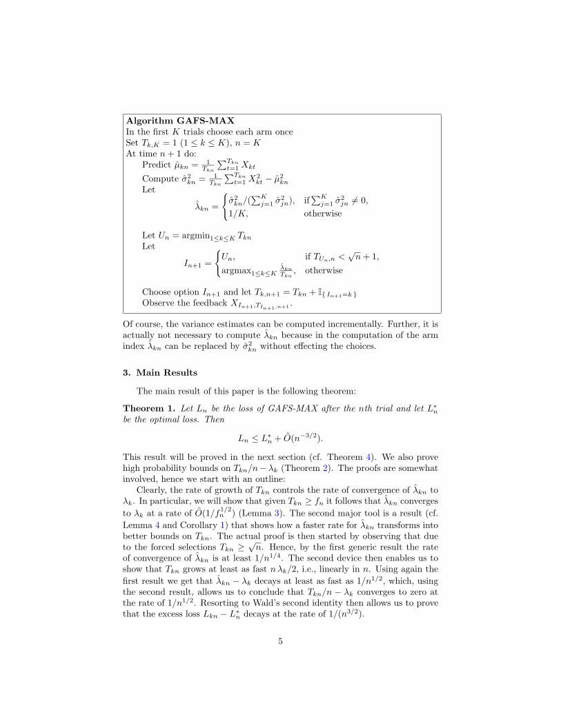
Algorithm GAFS-MAXIn the first K trials choose each arm onceSet Tk,K = 1 (1 ≤ k ≤ K), n = KAt time n+ 1 do:

Predict µkn = 1Tkn

∑Tknt=1 Xkt

Compute σ2kn = 1

Tkn

∑Tknt=1 X

2kt − µ2

kn

Let

λkn =

σ2kn/(

∑Kj=1 σ

2jn), if

∑Kj=1 σ

2jn 6= 0,

1/K, otherwise

Let Un = argmin1≤k≤K TknLet

In+1 =

Un, if TUn,n <

√n+ 1,

argmax1≤k≤KλknTkn

, otherwise

Choose option In+1 and let Tk,n+1 = Tkn + I In+1=k Observe the feedback XIn+1,TIn+1,n+1 .

Of course, the variance estimates can be computed incrementally. Further, it isactually not necessary to compute λkn because in the computation of the armindex λkn can be replaced by σ2

kn without effecting the choices.

3. Main Results

The main result of this paper is the following theorem:

Theorem 1. Let Ln be the loss of GAFS-MAX after the nth trial and let L∗nbe the optimal loss. Then

Ln ≤ L∗n + O(n−3/2).

This result will be proved in the next section (cf. Theorem 4). We also provehigh probability bounds on Tkn/n− λk (Theorem 2). The proofs are somewhatinvolved, hence we start with an outline:

Clearly, the rate of growth of Tkn controls the rate of convergence of λkn toλk. In particular, we will show that given Tkn ≥ fn it follows that λkn convergesto λk at a rate of O(1/f1/2

n ) (Lemma 3). The second major tool is a result (cf.Lemma 4 and Corollary 1) that shows how a faster rate for λkn transforms intobetter bounds on Tkn. The actual proof is then started by observing that dueto the forced selections Tkn ≥

√n. Hence, by the first generic result the rate

of convergence of λkn is at least 1/n1/4. The second device then enables us toshow that Tkn grows at least as fast nλk/2, i.e., linearly in n. Using again thefirst result we get that λkn − λk decays at least as fast as 1/n1/2, which, usingthe second result, allows us to conclude that Tkn/n − λk converges to zero atthe rate of 1/n1/2. Resorting to Wald’s second identity then allows us to provethat the excess loss Lkn − L∗n decays at the rate of 1/(n3/2).

5

The convergence rate statements for λkn and Tkn/n hold with high proba-bility. In particular, they all hold on the same event set Aδ.

4. Proof

The proof is developed through a series of Lemmata. First, we state Hoeffd-ing’s inequality in a form that suits the best our needs:

Lemma 1 (Hoeffding’s inequality, [10]). Let Zt be a sequence of zero-mean,i.i.d. random variables, where a ≤ Zt ≤ b, a < b reals. Then, for any 0 < δ ≤ 1,

P

(1n

n∑t=1

Zt >

√12

(b− a)2

nlog(1/δ)

)≤ δ.

Let us now introduce some notation. First, let

∆(R,n, δ) = R

√log(1/δ)

2n

denote the deviation bound that we can get from Hoeffding’s equality for theconfidence level δ after seeing n samples from a distribution whose supportis included in an interval of length R. Further, let µ(2)

k = E[X2kt

], Rk be

the length of the (connected) range of the random variables Xktt (i.e., Rk =esssupXkt−essinf Xkt), Sk be the length of the (connected) range of the randomvariables X2

ktt, and Bk be the essential supremum of the random variables|Xkt|t. Note that Rk ≤ 2Bk and Sk ≤ B2

k. Let

Aδ =⋂

1≤k≤K,n≥1

∣∣∣∣∣ 1nn∑t=1

X2kt − µ

(2)k

∣∣∣∣∣ ≤ ∆(Sk, n, δn)

∩

⋂1≤k≤K,n≥1

∣∣∣∣∣ 1nn∑t=1

Xkt − µk

∣∣∣∣∣ ≤ ∆(Rk, n, δn)

,

whereδn =

δ

4K(n(n+ 1).

Note that δn is chosen such that∑Kk=1

∑∞n=1 δn = δ/4. Hence, we observe that

by Hoeffding’s inequalityP (Aδ) ≥ 1− δ.

The sets Aδ will play a key role in the proof: Many of the statements will beproved on these set.

Our first result connects a lower bound on Tkn to the rate of convergenceof λkn. Let ak = |µk| + Bk, bk = Sk + akRk (≤ 5B2

k), a′k = 2bk/σ2k, and

`K,δ = log(4K/δ). Note that, by σ2k ≤ (Rk/2)2,

a′k ≥ 8bk/R2k ≥ 8ak/Rk ≥ 8Bk/Rk ≥ 4 (1)

6

and thatlog(δ−1

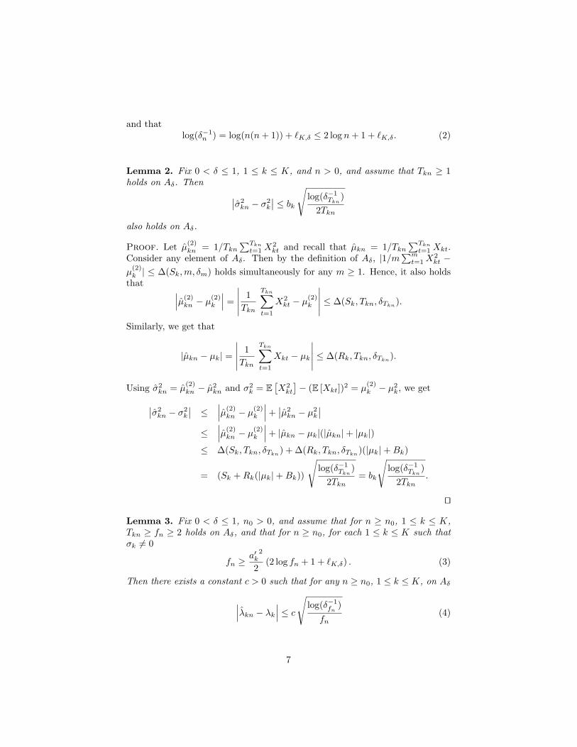
n ) = log(n(n+ 1)) + `K,δ ≤ 2 log n+ 1 + `K,δ. (2)

Lemma 2. Fix 0 < δ ≤ 1, 1 ≤ k ≤ K, and n > 0, and assume that Tkn ≥ 1holds on Aδ. Then ∣∣σ2

kn − σ2k

∣∣ ≤ bk√

log(δ−1Tkn

)2Tkn

also holds on Aδ.

Proof. Let µ(2)kn = 1/Tkn

∑Tknt=1 X

2kt and recall that µkn = 1/Tkn

∑Tknt=1 Xkt.

Consider any element of Aδ. Then by the definition of Aδ, |1/m∑mt=1X

2kt −

µ(2)k | ≤ ∆(Sk,m, δm) holds simultaneously for any m ≥ 1. Hence, it also holds

that ∣∣∣µ(2)kn − µ

(2)k

∣∣∣ =

∣∣∣∣∣ 1Tkn

Tkn∑t=1

X2kt − µ

(2)k

∣∣∣∣∣ ≤ ∆(Sk, Tkn, δTkn).

Similarly, we get that

|µkn − µk| =

∣∣∣∣∣ 1Tkn

Tkn∑t=1

Xkt − µk

∣∣∣∣∣ ≤ ∆(Rk, Tkn, δTkn).

Using σ2kn = µ

(2)kn − µ2

kn and σ2k = E

[X2kt

]− (E [Xkt])2 = µ

(2)k − µ2

k, we get∣∣σ2kn − σ2

k

∣∣ ≤ ∣∣∣µ(2)kn − µ

(2)k

∣∣∣+∣∣µ2kn − µ2

k

∣∣≤

∣∣∣µ(2)kn − µ

(2)k

∣∣∣+ |µkn − µk|(|µkn|+ |µk|)

≤ ∆(Sk, Tkn, δTkn) + ∆(Rk, Tkn, δTkn)(|µk|+Bk)

= (Sk +Rk(|µk|+Bk))

√log(δ−1

Tkn)

2Tkn= bk

√log(δ−1

Tkn)

2Tkn.

ut

Lemma 3. Fix 0 < δ ≤ 1, n0 > 0, and assume that for n ≥ n0, 1 ≤ k ≤ K,Tkn ≥ fn ≥ 2 holds on Aδ, and that for n ≥ n0, for each 1 ≤ k ≤ K such thatσk 6= 0

fn ≥a′k

2

2(2 log fn + 1 + `K,δ) . (3)

Then there exists a constant c > 0 such that for any n ≥ n0, 1 ≤ k ≤ K, on Aδ

∣∣∣λkn − λk∣∣∣ ≤ c√

log(δ−1fn

)fn

(4)

7

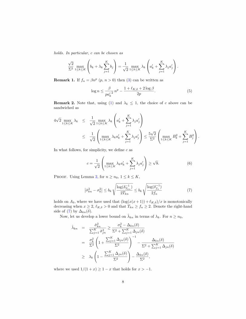
holds. In particular, c can be chosen as

√2

Σ2max

1≤k≤K

bk + λk

K∑j=1

bj

=1√2

max1≤k≤K

λk

a′k +K∑j=1

λja′j

.

Remark 1. If fn = βnp (p, n > 0) then (3) can be written as

log n ≤ β

pa′k2 n

p − 1 + `K,δ + 2 log β2p

. (5)

Remark 2. Note that, using (1) and λk ≤ 1, the choice of c above can besandwiched as

4√

2 max1≤k≤K

λk ≤ 1√2

max1≤k≤K

λk

a′k +K∑j=1

λja′j

≤ 1√

2

max1≤k≤K

λka′k +

K∑j=1

λja′j

≤ 5√

2Σ2

max1≤k≤K

B2k +

K∑j=1

B2j

.

In what follows, for simplicity, we define c as

c =1√2

max1≤k≤K

λka′k +

K∑j=1

λja′j

≥ √8. (6)

Proof. Using Lemma 2, for n ≥ n0, 1 ≤ k ≤ K,

∣∣σ2kn − σ2

k

∣∣ ≤ bk√

log(δ−1Tkn

)2Tkn

≤ bk

√log(δ−1

fn)

2fn(7)

holds on Aδ, where we have used that (log(x(x+ 1)) + `K,δ)/x is monotonicallydecreasing when x ≥ 2, `K,δ > 0 and that Tkn ≥ fn ≥ 2. Denote the right-handside of (7) by ∆kn(δ).

Now, let us develop a lower bound on λkn in terms of λk. For n ≥ n0,

λkn =σ2kn∑K

j=1 σ2jn

≥ σ2k −∆kn(δ)

Σ2 +∑Kj=1 ∆jn(δ)

=σ2k

Σ2

(1 +

∑Kj=1 ∆jn(δ)

Σ2

)−1

− ∆kn(δ)

Σ2 +∑Kj=1 ∆jn(δ)

≥ λk

(1−

∑Kj=1 ∆jn(δ)

Σ2

)− ∆kn(δ)

Σ2,

where we used 1/(1 + x) ≥ 1− x that holds for x > −1.

8

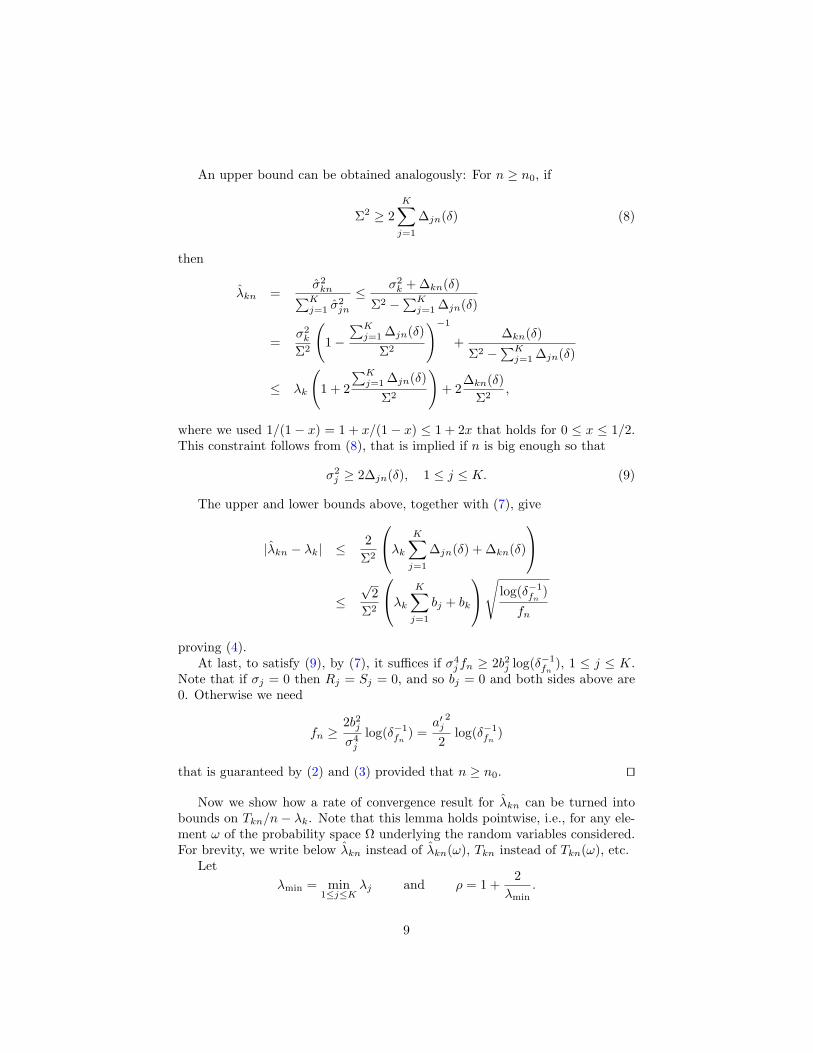
An upper bound can be obtained analogously: For n ≥ n0, if

Σ2 ≥ 2K∑j=1

∆jn(δ) (8)

then

λkn =σ2kn∑K

j=1 σ2jn

≤ σ2k + ∆kn(δ)

Σ2 −∑Kj=1 ∆jn(δ)

=σ2k

Σ2

(1−

∑Kj=1 ∆jn(δ)

Σ2

)−1

+∆kn(δ)

Σ2 −∑Kj=1 ∆jn(δ)

≤ λk

(1 + 2

∑Kj=1 ∆jn(δ)

Σ2

)+ 2

∆kn(δ)Σ2

,

where we used 1/(1− x) = 1 + x/(1− x) ≤ 1 + 2x that holds for 0 ≤ x ≤ 1/2.This constraint follows from (8), that is implied if n is big enough so that

σ2j ≥ 2∆jn(δ), 1 ≤ j ≤ K. (9)

The upper and lower bounds above, together with (7), give

|λkn − λk| ≤2

Σ2

λk K∑j=1

∆jn(δ) + ∆kn(δ)

≤√

2Σ2

λk K∑j=1

bj + bk

√ log(δ−1fn

)fn

proving (4).At last, to satisfy (9), by (7), it suffices if σ4

j fn ≥ 2b2j log(δ−1fn

), 1 ≤ j ≤ K.Note that if σj = 0 then Rj = Sj = 0, and so bj = 0 and both sides above are0. Otherwise we need

fn ≥2b2jσ4j

log(δ−1fn

) =a′j

2

2log(δ−1

fn)

that is guaranteed by (2) and (3) provided that n ≥ n0. ut

Now we show how a rate of convergence result for λkn can be turned intobounds on Tkn/n− λk. Note that this lemma holds pointwise, i.e., for any ele-ment ω of the probability space Ω underlying the random variables considered.For brevity, we write below λkn instead of λkn(ω), Tkn instead of Tkn(ω), etc.

Letλmin = min

1≤j≤Kλj and ρ = 1 +

2λmin

.

9

In what follows, unless otherwise stated, we will assume that λmin > 0. ForK = 1 the results are obvious, so without the loss of generality (w.l.o.g.) we canalso assume that K ≥ 2, in which case λmin ≤ 1/K ≤ 1/2 and 5 ≤ ρ ≤ 2.5/λmin.

Lemma 4. Fix n0 > 0. Assume that gn is such that for n ≥ n0, ngn ismonotone increasing, 5ngn ≥ d

√ne, and

gn ≤ λmin/2, (10)

|λkn − λk| ≤ gn, 1 ≤ k ≤ K (11)

hold. Then the following inequalities hold for n ≥ 1 and 1 ≤ k ≤ K:

−(K − 1) max(n0

n,

1n

+ ρgn

)≤ Tkn

n− λk ≤ max

(n0

n,

1n

+ ρgn

).

Proof. By definition Tk,n+1 = Tkn + I In+1=k . Let Ekn = Tkn − nλk withEk0 = 0. Note that Ekn ≤ n(1− λk) and

K∑k=1

Ekn = 0 (12)

hold for any n ≥ 0. Notice that the desired result can be stated as bounds onEkn. Hence, our goal now is to study Ekn. If bjn is an upper bound for Ejn(1 ≤ j ≤ K) then from (12) we get the lower bound Ekn = −

∑j 6=k Ejn ≥

−∑j 6=k bjn ≥ −(K − 1) maxj bjn. Hence, we target upper bounds on Eknk.

Assume now that n ≥ n0. Note that (10) and (11) imply λk − λkn ≤|λkn − λk| ≤ λk/2, and thus λkn ≥ λk/2 > 0 for each k.

From the definition of Ekn and Tkn we get

Ek,n+1 = Ekn − λk + I In+1=k .

By the definition of the algorithm

I In+1=k ≤ ITkn≤d

√ne or k=argmin1≤j≤K

Tjn

λjn

ff,

Assume now that k is an index where Tjnλjnj takes its minimum, that is,

Tkn

λkn≤ min

j

Tjn

λjn.

Using Tjn = Ejn + nλj and reordering the terms gives

Ekn + nλk ≤ λkn minj

Ejn + nλj

λjn≤ λkn

(minj

Ejn

λjn+ nmax

j

λj

λjn

).

10

By (12), there exists an index j such that Ejn ≤ 0. Since λjn > 0 for any j, itholds that minj

Ejn

λjn≤ 0. Hence,

Ekn + nλk ≤ nλkn maxj

λj

λjn. (13)

Using (11) and (10), we get

λj

λjn≤ λjλj − gn

=1

1− gn/λj.

This is upper bounded by

1 +2gnλj

using 1/(1 − x) ≤ 1 + 2x for 0 ≤ x ≤ 1/2, where the latest constraint followsfrom (10). Using (13), λkn ≤ 1,and (11) again,

Ekn ≤ nλkn maxj

λj

λjn− nλk

≤ n(λkn − λk) +2ngnλmin

≤(

1 +2

λmin

)ngn = ρngn.

Denote the right-hand side by Fn. Hence,

I In+1=k ≤ ITkn≤d√ne or Ekn≤Fn .

We show that Tkn ≤ d√ne implies Ekn ≤ Fn. By the definition of Ekn, from

Tkn ≤ d√ne it follows that Ekn = Tkn−nλk ≤ d

√ne ≤ 5ngn. The bound ρ ≥ 5

implies 5ngn ≤ Fn. Hence, Ekn ≤ Fn follows. Therefore

I In+1=k ≤ IEkn≤Fn .

Now we need the following technical lemma:

Lemma 5. Let 0 ≤ λ ≤ 1. Consider the sequences En, En, In, In (n ≥ 1) whereIn, In ∈ 0, 1, En+1 = En + In − λ, En+1 = En + In − λ, E1 = E1 and assumethat In ≤ In holds whenever En = En. Then En ≤ En holds for n ≥ 1.

Proof. Consider the difference sequence Pn = En − En. The goal is to showthat Pn ≥ 0 holds for any n. It holds that P1 = 0. Since

Pn+1 − Pn = (En+1 − En)− (En+1 − En) = In − In ∈ −1, 0,+1 ,

Pn is always an integer. Hence, it suffices to show that Pn+1 ≥ 0 if Pn = 0.However, this holds because if Pn = 0 then In ≤ In. ut

11

Now, returning to the proof of Lemma 4, define Eknn≥n0 by

Ek,n0 = Ek,n0 ,

Ek,n+1 = Ekn − λk + I Ekn≤Fn , n ≥ n0.

The conditions of Lemma 5 are clearly satisfied from index n0. ConsequentlyEkn ≤ Ekn holds for any n ≥ n0. Further, since Fn is monotone increasing inn,

Ekn ≤ max(Ek,n0 , 1 + Fn) ≤ max(n0(1− λk), 1 + Fn), n ≥ n0,

and so Ekn ≤ max(n0(1 − λk), 1 + Fn) ≤ max(n0, 1 + Fn) for n ≥ 0, finishingthe upper-bound. ut

Corollary 1. Fix 0 < δ ≤ 1, c ≥ 1/5, and n0 ≥ 1. Assume that fn > 0 is suchthat for n ≥ n0, fn is monotone increasing, but fn/n2 is monotone decreasing,1 ≤ fn ≤ n,

fn ≥4c2

λ2min

(2 log fn + 1 + `K,δ), and (14)

|λkn − λk| ≤ c

√log(δ−1

fn)

fn, 1 ≤ k ≤ K (15)

hold. Let Fn(δ) = ρngn(δ), where

gn(δ) = c

√log(δ−1

fn)

fn.

Then the following inequalities hold for n ≥ 0 and 1 ≤ k ≤ K:

−(K − 1) max(n0, 1 + Fn(δ)) ≤ Tkn − nλk ≤ max(n0, 1 + Fn(δ)).

Further, these inequalities remain valid if δfn is replaced by δn in Fn(δ).

Remark 3. If fn = βnp (p,n > 0) then (14) can be written as

log n ≤ βλ2min

8pc2np − 1 + `K,δ + 2 log β

2p. (16)

Proof. Assume that n ≥ n0. Then ngn(δ) is monotone increasing, (2) and(14) imply (10), and (15) implies (11). The bounds on fn, K, and δ imply

5ngn(δ) = 5nc

√log(4Kfn(fn + 1)/δ)

fn≥ 5c

√n log(8fn0(fn0 + 1)),

that is at least√n log(16) >

√2n ≥ d

√ne by the bounds on c and fn0 . Thus

Lemma 4 gives the result. The last statement follows obviously from δ−1fn≤ δ−1

n

(since fn ≤ n). ut

12

Using the previous results we are now in the position to prove a linear lowerbound on Tkn:

Lemma 6. Let 0 < δ ≤ 1 arbitrary. Then there exists an integer N1 such thatfor any n ≥ N1, 1 ≤ k ≤ K, Tkn ≥ nλk/2 holds on Aδ.

In particular,

N1 = max

(2(K − 1)λmin

n′0, D42

[logD4

2 +12(`K,δ + 1 + 7 · 10−9

)]2), (17)

where D2 = 4c(2K − 1)/λ2min, c is defined by (6), and

n′0 = max(K(K + 1), n1, n2),

n1 = max1≤k≤K

a′k4 [4 log a′k + 1 + `K,δ]

2,

n2 = 4(

2cλmin

)4[

4 log

(√8c

λmin

)+ 1 + `K,δ

]2

.

For the proof we need the following technical lemma that gives a bound onthe point when for a > 0 the function at1/2 + b overtakes log t.

Lemma 7. Let a > 0. For any t ≥ (2/a)2[log((2/a)2)− b

]2, at1/2 + b ≥ log t.

The proof of this lemma can be found in Appendix B.

Proof (Lemma 6). Due to the forced selection of the options built into thealgorithm, Tkn ≥

√n holds for n ≥ K(K + 1). The proof of this statement

is somewhat technical and is moved into the Appendix A (Lemma 11). ByLemma 7, for

n ≥ n1 = max1≤k≤K

a′k4 [4 log a′k + 1 + `K,δ]

2,

(5) holds with p = 1/2, β = 1 for each k. Hence, we can apply Lemma 3 andRemark 1 following it with n0 = max(K(K + 1), n1) and fn = n1/2 (≥ 2), andget that ∣∣∣λkn − λk∣∣∣ ≤ c

√log(δ−1

n1/2)n1/2

(18)

on Aδ for n ≥ n0, 1 ≤ k ≤ K, and c ≥√

8 as defined by (6). By Lemma 7again, for

n ≥ n2 = 4(

2cλmin

)4[

4 log

(√8c

λmin

)+ 1 + `K,δ

]2

,

(16) holds with p = 1/2, β = 1. Now, we can apply Corollary 1 and Remark 3following it on Aδ with n′0 = max(n0, n2) = max(K(K + 1), n1, n2) and fn =n1/2 (≥ 1), and get that on Aδ for n ≥ 0, 1 ≤ k ≤ K,

Tkn ≥ nλk − (K − 1) max(n′0, 1 +Hn(δ)),

13

whereHn(δ) = D1n

3/4√

log(δ−1n )

and D1 = cρ. Hence, Tkn ≥ nλk/2 by the time when n ≥ 2n′0(K − 1)/λmin andn ≥ 2(K−1)(1+Hn(δ))/λmin. These two constrains are satisfied when n ≥ N1,where N1 is defined as in equation (17); the first one is obvious, the second onefollows from Proposition 7 in Appendix C. ut

With the help of this result we can get better bounds on Tkn, resulting inour first main result:

Theorem 2. Let 0 < δ ≤ 1 be arbitrary. Then there exists an integer N2 anda positive real number D3 such that for any n ≥ 0, 1 ≤ k ≤ K,

−(K − 1) max(N2, 1 +Gn(δ)) ≤ Tkn − nλk ≤ max(N2, 1 +Gn(δ))

holds on Aδ, where

Gn(δ) = D3

√n log(δ−1

n ).

In particular, D3 = cρ√

2/λmin, c is defined by (6),

N2 = max(N1, n′1, n′2),

where N1 is defined in Lemma 6, and

n′1 = max1≤k≤K

2a′k2

λmin[4 log a′k + 1 + `K,δ] ,

n′2 =(4c)2

λ3min

[4 log

√8c

λmin+ 1 + `K,δ

].

The theorem shows that asymptotically the GAFS-MAX algorithm behavesthe same way as an optimal allocation rule that knows the variances. It alsoshows that the deviation of the proportion of choices of any option from theoptimal value decays as O(1/

√n).

For the proof we need the counterpart of Lemma 7 for linear functions. Theproof is in Appendix B.

Lemma 8. Let a > 0. Then for any t ≥ (2/a)[log(1/a)− b], at+ b ≥ log t.

Proof (Theorem 2). The proof is almost identical to that of Lemma 6. Thedifference is that now we start with a better lower bound on Tkn. In particular,by Lemma 6, Tkn ≥ nλk/2 ≥ nλmin/2 holds on Aδ for n ≥ N1. By Lemma 8,for

n ≥ n′1 = max1≤k≤K

2a′k2

λmin[4 log a′k + 1 + `K,δ] ,

14

(5) holds with p = 1, β = λmin/2 for each k. Hence, we can apply Lemma 3and Remark 1 following it with n′0 = max(N1, n

′1) and fn = nλmin/2 (≥ 2), and

get that ∣∣∣λkn − λk∣∣∣ ≤ c√

2 log(δ−1nλmin/2

)

nλmin(19)

on Aδ for n ≥ n′0, 1 ≤ k ≤ K, and c ≥√

8 as defined by (6). By Lemma 8again, for

n ≥ n′2 =(4c)2

λ3min

[4 log

√8c

λmin+ 1 + `K,δ

],

(16) holds with p = 1, β = λmin/2. Now, we can apply Corollary 1 and Remark 3following it on Aδ with (n0 =)N2 = max(n′0, n

′2) = max(N1, n

′1, n′2) and fn =

nλmin/2 (≥ 1), and get that on Aδ for n ≥ 0, 1 ≤ k ≤ K,

−(K − 1) max(N2, 1 +Gn(δ)) ≤ Tkn − nλk ≤ max(N2, 1 +Gn(δ)),

whereGn(δ) = D3

√n log(δ−1

n )

and D3 = cρ√

2/λmin. ut

This result yields a bound on the expected value of E [Tkn]:

Theorem 3. Let N ′2 = sup0<δ≤1N2/`2K,δ, where N2 is defined in Theorem 2.

Then, N ′2 < ∞ and there exists an index N3 that depends only on N ′2, 1/D3,and logK polynomially, such that for any k and n ≥ N3,

E [Tkn] ≤ nλk +D3

√n(1 + log(4Kn(n+ 1))) + 2. (20)

Proof. Recalling the definition of N2 and that `K,δ ≥ log 8, we can see easilythat N ′2 < ∞. Note that N ′2 does not depend on δ, and N2 ≤ N ′2`

2K,δ ≤

N ′2 log2(δ−1n ) holds for any 0 < δ ≤ 1. Fix 0 < δ ≤ 1. If n ≥ N2

2 /(D23 log(δ−1

n )),then 1 +Gn(δ) ≥ N2, thus it follows from Theorem 2 that for such n,

P(Tkn − nλk − 1

D3n1/2>

√log(δ−1

n ))≤ δ,

where we used P (Aδ) ≥ 1 − δ. Let Z = (Tkn − nλk − 1)/(D3n1/2) and

t =√

log(δ−1n ). The above inequality is equivalent to

P (Z > t) ≤ 4Kn(n+ 1) e−t2.

By the constraint that connects n and δ, this inequality holds for any pair (n, t)that satisfy

n ≥ N ′22 log3(δ−1

n )/D23 = N ′2

2t6/D2

3,

15

that is, for any (n, t) such that

t ≤ (nD23/N

′22)1/6.

Also, since Z ≤ n1/2/D3 is always true, P (Z > t) = 0 holds for t ≥ n1/2/D3.We need the following technical lemma, a variant of which can be found, e.g.,as Exercise 12.1 in [7]:

Lemma 9. Let C > 1, c > 0, 0 < a ≤ b. Assume that the random variableZ satisfies P (Z > t) ≤ C exp(−ct2) for any t ≤ a, and P (Z > t) = 0 for anyt ≥ b. Then

E [Z] ≤√

(1 + logC)/c+ Cb2e−ca2 . (21)

Proof. By the monotonicity of P (Z > t) ≤ 1, for any u > 0,

E[Z2]

=∫ ∞

0

P(Z2 > t

)dt =

∫ u

0

+∫ a2

u

+∫ b2

a2+∫ ∞b2

≤ u+

(∫ a2

u

Ce−ct dt

)+

+∫ b2

a2P (Z > a) dt+ 0

≤ u+C

c

(e−cu − e−ca

2)+

+ (b2 − a2)Ce−ca2.

This gives

E[Z2]≤ min

(1 + logC − Ce−ca2

c, a2

)+(b2−a2)Ce−ca

2≤ 1 + logC

c+Cb2e−ca

2

with the choice u = min((logC)/c, a2). Now,

E [Z] ≤√

E [Z2] ≤√

1 + logCc

+ Cb2e−ca2 . ut

Applying Lemma 9 with a = (nD23/N

′22)1/6, b = n1/2/D3, C = 4Kn(n+ 1),

and c = 1,

E [Z] ≤√

1 + log(4Kn(n+ 1)) + 4Kn2(n+ 1)e−(nD23/N

′22)1/3/D2

3.

Thus

E [Tkn] ≤ 1 + nλk

+√D2

3n(1 + log(4Kn(n+ 1))) + 4Kn3(n+ 1)e−(nD23/N

′22)1/3 .

Equation (20) then follows by straightforward algebra. ut

In order to develop a bound on the loss Lkn we need Wald’s (second) identity:

16

Lemma 10 (Wald’s Identity, Theorem 13.2.14 of [2]). Let Ft be a fil-tration and let Yt be an Ft-adapted sequence of i.i.d. random variables. As-sume that Ft and σ(Ys : s ≥ t+ 1 ) are independent and T is a stoppingtime w.r.t. Ft with a finite expected value: E [T ] < +∞. Consider the partialsums Sn = Y1 + . . .+ Yn, n ≥ 1. If E

[Y 2

1

]< +∞ then

E[(ST − TE [Y1])2

]= Var [Y1] E [T ] . (22)

The following theorem is the main result of the paper:

Theorem 4. Fix k. Then

Ln ≤ L∗n + O(n−3/2).

Proof. Let Skn =∑nt=1Xkt,

Lkn =Sk,Tkn − Tknµk

Tkn,

G′n(δ) = (K − 1) max(N2, 1 +Gn(δ)) and

G′′n = D3

√n(1 + log(4Kn(n+ 1))) + 2.

Note that by Theorem 2,

P (Tkn < nλk −G′n(δ)) ≤ δ (23)

holds for any n ≥ 0 and 0 < δ ≤ 1. Then, for any 0 < δ ≤ 1,

Lkn = E[L2kn

]= E

[L2knITkn≥nλk−G′n(δ)

]+ E

[L2knITkn<nλk−G′n(δ)

]≤

E[(Sk,Tkn − Tknµk)2

](nλk −G′n(δ))2

+R2k P (Tkn < nλk −G′n(δ)) .

Using Lemma 10 and then (20) of Theorem 3 for the first term, for n ≥ N3,

E[(Sk,Tkn − Tknµk)2

]= σ2

kE [Tkn] ≤ σ2k(nλk +G′′n),

and thus

E[(Sk,Tkn − Tknµk)2

](nλk −G′n(δ))2

≤ σ2k(nλk +G′′n)

(nλk −G′n(δ))2

=σ2k

nλk

1(1−G′n(δ)/(nλk))2

+σ2kG′′n

(nλk −G′n(δ))2,

while, by (23), the second term is bounded above by R2kδ.

Now choose δ = n−3/2. Then, recalling the definition of G′n(δ), Gn(δ), δn,`K,δ, and that N2 ≤ N ′2`

2K,δ, we have G′n(n−3/2) = O(

√n log n), thus for n

17

sufficiently large, G′n(n−3/2)/(nλk) ≤ 1/2. Therefore, for such large n, using1/(1− x) ≤ 1 + 2x for 0 ≤ x ≤ 1/2, we get,

Lkn ≤ σ2k

nλk

(1 + 2

G′n(n−3/2)nλk

)2

+σ2kG′′n

(nλk −G′n(n−3/2))2+R2

kn−3/2,

which gives

Lkn ≤σ2k

nλk+ O(n−3/2) =

Σ2

n+ O(n−3/2) = L∗n + O(n−3/2).

Taking the maximum with respect to k yields the desired result. ut

Let us now comment on the case when for some options λk = 0. Such armsare chosen in the optimal allocation exactly once. Algorithm GAFS-MAX willselect such options

√n-times in n-steps since the estimated variance will be zero.

Hence, we will have Tkn ≤ T ∗kn + O(√n). Clearly, the loss for such an option

will be zero. Further, since options with σ2k = 0 are pulled only O(

√n)-times,

they can not significantly influence the number of times the other options arechosen. Hence, the results go through if we replace mink λk with mink:λk 6=0 λk.

5. Illustration

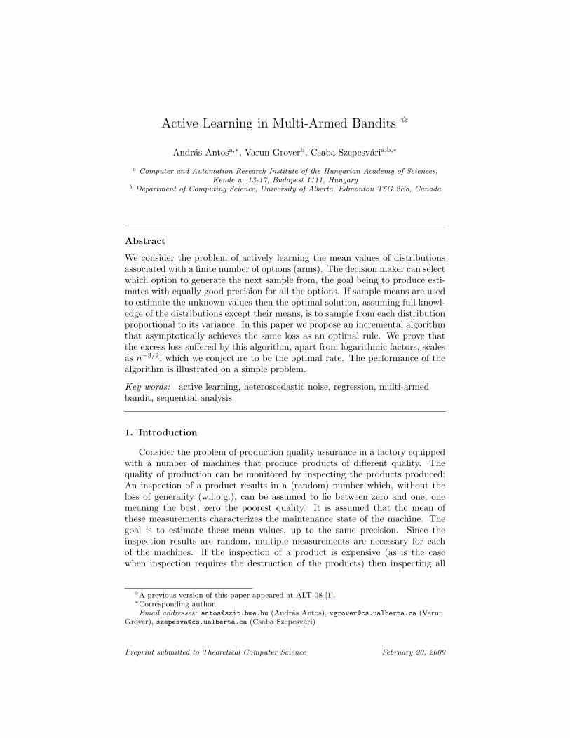
The purpose of this section is to illustrate the theory by means of somecomputer experiments. One particular goal of the experiments was to verify theexcess loss rate obtained in the previous section. Another goal was to comparethe adaptive strategy with a non-adaptive strategy.

5.1. Experimental SetupHere we illustrate the behavior of the algorithm in a simple problem with

K = 2, when the random responses modeled as Bernoulli random variables foreach of the options. In order to estimate the expected squared loss between thetrue mean and the estimated mean we repeat the experiment 100,000 times,then take the average. The error bars shown on the graphs show the standarddeviations of these averages. The algorithms compared are GAFS-MAX (the al-gorithm studied here), GFSP-MAX (the algorithm described in the introductionthat works in phases), and “UNIF”, the uniform allocation rule.

5.2. ResultsIn order for an adaptive algorithm to have any advantage the two options

have to have different variances. For this purpose we chose p1 = 0.8, p2 = 0.9so that λ1 = 0.64 and λ2 = 0.36.

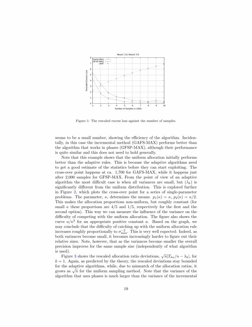
Figure 1 shows the rescaled excess loss, n3/2(Ln − L∗n), for the three algo-rithms. We see that the rescaled excess losses of the adaptive algorithms staybounded, as predicted by the theory, while the rescaled loss of the uniform sam-pling strategy grows as

√n. It is remarkable that the limit of the rescaled loss

18

0

1

2

3

4

5

6

7

8

1 2 3 4 5 6 7 8 9 10

Res

cale

d E

xces

s Lo

ss

Number of Samples (x 1000)

Mean1: 0.8, Mean2: 0.9

GAFS-MAXGFSP-MAX

UNIF

Figure 1: The rescaled excess loss against the number of samples.

seems to be a small number, showing the efficiency of the algorithm. Inciden-tally, in this case the incremental method (GAFS-MAX) performs better thanthe algorithm that works in phases (GFSP-MAX), although their performanceis quite similar and this does not need to hold generally.

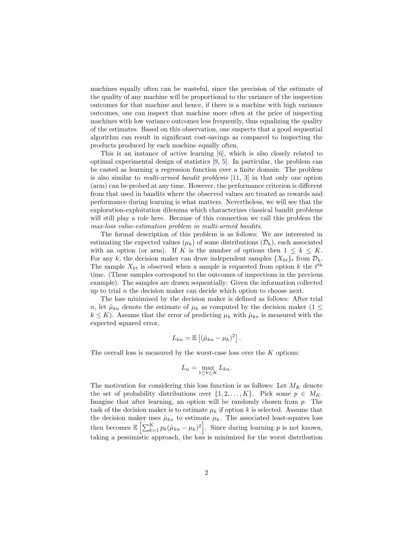
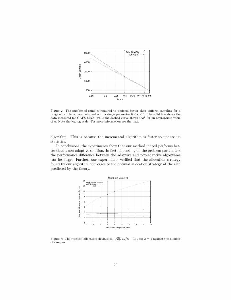
Note that this example shows that the uniform allocation initially performsbetter than the adaptive rules. This is because the adaptive algorithms needto get a good estimate of the statistics before they can start exploiting. Thecross-over point happens at ca. 1,700 for GAFS-MAX, while it happens justafter 2,000 samples for GFSP-MAX. From the point of view of an adaptivealgorithm the most difficult case is when all variances are small, but (λk) issignificantly different from the uniform distribution. This is explored furtherin Figure 2, which plots the cross-over point for a series of single-parameterproblems. The parameter, κ, determines the means: p1(κ) = κ, p2(κ) = κ/2.This makes the allocation proportions non-uniform, but roughly constant (forsmall κ these proportions are 4/5 and 1/5, respectively for the first and thesecond option). This way we can measure the influence of the variance on thedifficulty of competing with the uniform allocation. The figure also shows thecurve a/κ2 for an appropriate positive constant a. Based on the graph, wemay conclude that the difficulty of catching up with the uniform allocation ruleincreases roughly proportionally to σ−2

max. This is very well expected: Indeed, asboth variances become small, it becomes increasingly harder to figure out theirrelative sizes. Note, however, that as the variances become smaller the overallprecision improves for the same sample size (independently of what algorithmis used).

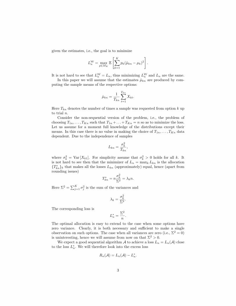
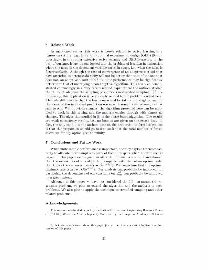
Figure 3 shows the rescaled allocation ratio deviations,√n|Tkn/n− λk|, for

k = 1. Again, as predicted by the theory, the rescaled deviations stay boundedfor the adaptive algorithms, while, due to mismatch of the allocation ratios, itgrows as

√n for the uniform sampling method. Note that the variance of the

algorithm that uses phases is much larger than the variance of the incremental

19

500

1000

2000

4000

8000

0.15 0.2 0.25 0.3 0.35 0.4 0.45 0.5

Cat

ch-u

p tim

e

kappa

GAFS-MAXa/kappa2

Figure 2: The number of samples required to perform better than uniform sampling for arange of problems parameterized with a single parameter 0 < κ < 1. The solid line shows thedata measured for GAFS-MAX, while the dashed curve shows a/κ2 for an appropriate valueof a. Note the log-log scale. For more information see the text.

algorithm. This is because the incremental algorithm is faster to update itsstatistics.

In conclusions, the experiments show that our method indeed performs bet-ter than a non-adaptive solution. In fact, depending on the problem parametersthe performance difference between the adaptive and non-adaptive algorithmscan be large. Further, our experiments verified that the allocation strategyfound by our algorithm converges to the optimal allocation strategy at the ratepredicted by the theory.

-2

0

2

4

6

8

10

12

14

1 2 3 4 5 6 7 8 9 10

Res

cale

d A

lloca

tion

devi

atio

n fo

r k=

1

Number of Samples (x 1000)

Mean1: 0.8, Mean2: 0.9

GAFS-MAXGFSP-MAX

UNIF

Figure 3: The rescaled allocation deviations,√n|Tkn/n − λk|, for k = 1 against the number

of samples.

20

6. Related Work

As mentioned earlier, this work is closely related to active learning in aregression setting (e.g., [4]) and to optimal experimental design (OED) [9]. In-terestingly, in the rather extensive active learning and OED literature, to thebest of our knowledge, no one looked into the problem of learning in a situationwhere the noise in the dependent variable varies in space, i.e., when the noise isheteroscedastic. Although the rate of convergence of an adaptive method thatpays attention to heteroscedasticity will not be better than that of the one thatdoes not, an adaptive algorithm’s finite-time performance may be significantlybetter than that of underlying a non-adaptive algorithm. This has been demon-strated convincingly in a very recent related paper where the authors studiedthe utility of adapting the sampling proportions in stratified sampling [8].2 In-terestingly, this application is very closely related to the problem studied here.The only difference is that the loss is measured by taking the weighted sum ofthe losses of the individual prediction errors with some fix set of weights thatsum to one. With obvious changes, the algorithm presented here can be mod-ified to work in this setting and the analysis carries through with almost nochanges. The algorithm studied in [8] is the phase-based algorithm. The resultsare weak consistency results, i.e., no bounds are given on the excess loss. Infact, the only condition the authors pose on the proportion of forced selectionsis that this proportion should go to zero such that the total number of forcedselections for any option goes to infinity.

7. Conclusions and Future Work

When finite sample performance is important, one may exploit heteroscedas-ticity to allocate more samples to parts of the input space where the variance islarger. In this paper we designed an algorithm for such a situation and showedthat the excess loss of this algorithm compared with that of an optimal rule,that knows the variances, decays as O(n−3/2). We conjecture that the optimalminimax rate is in fact O(n−3/2). Our analysis can probably be improved. Inparticular, the dependence of our constants on λ−1

min can probably be improvedby a great extent.

Although in this paper we have not considered the full non-parametric re-gression problem, we plan to extend the algorithm and the analysis to suchproblems. We also plan to apply the technique to stratified sampling and otherrelated problems.

Acknowledgements

This research was funded in part by the National Science and Engineering Research Coun-

cil (NSERC), iCore, the Alberta Ingenuity Fund, and by the Hungarian Academy of Sciences

2In fact, we have learned about this paper just at the time when we submitted the firstversion of this paper.

21

(Bolyai Fellowship for Andras Antos).

A. Forced selection lemma

Lemma 11. For 1 ≤ k ≤ K, n ≥ K(K + 1)

Tkn ≥√n (24)

holds.

Proof. For a positive integer l, let Cl =

(l − 1)2 + 1, (l − 1)2 + 2, . . . , l2

, apartition of 1, 2, . . . . Observe that if (24) holds for some n = n′ ∈ Cl, then itholds also for any n = n′′ ∈ Cl, n′′ > n′, since Tk,n′′ ≥ Tk,n′ ≥

√n′ > l−1 which

implies Tk,n′′ ≥ l ≥√n′′. Thus, it is enough to prove (24) for n = K(K + 1)

and then for n = l2 + 1, l = K + 1,K + 2, . . ..By a careful analysis of the algorithm, we see that only forced selection steps

happen till n = K(K + 2) in a uniform manner, during which each option isselected K + 2 times. This implies that Tk,K(K+1) = K + 1 >

√K(K + 1)

and that Tk,(K+1)2+1 ≥ Tk,K(K+2) = K + 2 >√

(K + 1)2 + 1, i.e., (24) holdsfor n = K(K + 1) and (K + 1)2 + 1, for all k. Now we use induction for l.Assume that (24) holds for all k, for some n = (l − 1)2 + 1 (l ≥ K + 2), i.e.,Tk,(l−1)2+1 ≥

√(l − 1)2 + 1 > l − 1 implying Tk,(l−1)2+1 ≥ l. Now at times

(l − 1)2 + 2, . . . , l2 + 1 (which total up to |Cl| = 2l − 1(≥ 2K − 3) steps), oneof those arms for which Tk,(l−1)2+1 = l holds is forced to be selected exactlyonce. Hence each such arm is selected at least once in this phase, assuringTk,l2+1 ≥ l + 1 >

√l2 + 1 for all k, i.e., (24) holds for n = l2 + 1. ut

B. Some elementary comparison lemmata

The purpose of this section is to provide upper bounds on the solutions ofequations of the form

log(t) = atp + b, (25)

where a, p, t > 0.Let

`(t) = log t,q(t) = atp + b, andt0 = (pa)−1/p.

Here t0 is the point where ` and q have the same growth rate, i.e., where`′(t0) = q′(t0). Note that for t ≥ t0, q′(t) ≥ `′(t). Hence, if q(t0) > `(t0)then (25) has no solutions on [t0,∞). Now observe that it also holds thatq′(t) ≤ `′(t) when t ≤ t0. Hence, if q(t0) > `(t0) then (25) has no solutionson (0, t0] since ` decreases faster than q as we move from t0 towards zero.Now, consider the case when q(t0) ≤ `(t0). Since for t ≥ t0, q′(t) ≥ `′(t) andq(t)/`(t) t→∞→ ∞, (25) will have exactly one solution in [t0,∞).

These findings are summarized in the next proposition:

22

Proposition 1. Consider t0 = (pa)−1/p, q(t) = atp+b and `(t) = log(t), wherea, p, t > 0. Then q(t0) ≤ `(t0) is a sufficient and necessary condition for theexistence of a solution to q(t) = `(t). Further, when q(t0) ≤ `(t0) then there isexactly one solution on [t0,∞).

Remark 4. Note that q(t0) ≤ `(t0) is equivalent to 1 + bp ≤ − log(pa), whichis thus a sufficient and necessary condition for the existence of a solution toq(t) = `(t).

In the sequel we will derive upper bounds on the solutions of (25) by pickingsome t∗ such that q(t∗) ≥ `(t∗) and q′(t∗) ≥ `′(t∗). In doing so we will firstconsider the homogeneous version of (25),

log u = a′up. (26)

The following proposition gives the link between the solutions of the homoge-neous and inhomogeneous equations.

Proposition 2. Any solution of (25) can be obtained by solving (26) with a′ =aepb and then using t = ebu and vice versa. Further, if u∗ is an upper bound onthe solutions of (26) then t∗ = ebu∗ is an upper bound on the solutions of (25).

Now, let us consider the linear case, i.e., when p = 1.

Proposition 3. Let t∗ = 2/a log(1/a), q(t) = at, `(t) = log t, where a > 0.Then for any positive t satisfying t ≥ t∗, q(t) ≥ `(t) holds.

Proof. We may assume that log(1/a) ≥ 1, or by Remark 4 q(t) = `(t) doesnot have a solution and the statement follows trivially. It suffices to verifythat `(t∗) ≤ q(t∗) and `′(t∗) ≤ q′(t∗). The second inequality follows fromlog(1/a) ≥ 1, the first follows from the inequality log(z2) ≤ z, which holds forany z > 0. ut

Proposition 4. Consider q(t) = at + b, `(t) = log(t), where a > 0. Let t∗ =2/a [−b+ log(1/a)]. Then for any positive t such that t ≥ t∗ it holds that q(t) ≥`(t).

Proof. The statement follows immediately from Propositions 2 and 3. ut

Proposition 5. Consider q(t) = at1/2, `(t) = log t. Let t∗ = (2/a)2 log2 (2/a)2.Then for any positive t such that t ≥ t∗, q(t) ≥ `(t) holds.

Proof. By Remark 4, q(t) = `(t) has a solution iff log(2/a) ≥ 1. Hence, weshall assume w.l.o.g. that this holds. It is easy to show then that `(t∗) ≤ q(t∗)and `′(t) ≤ q′(t) hold for t ≥ t∗. In particular, the first inequality follows fromlog(z2) ≤ z (z > 0), while the second inequality follows from log(2/a) ≥ 1. ut

Proposition 6. Consider q(t) = at1/2 + b, `(t) = log(t), where a > 0. Lett∗ = (2/a)2

[−b+ log (2/a)2

]2. Then for any positive t such that t ≥ t∗ it holdsthat q(t) ≥ `(t).

Proof. The statement follows immediately from Propositions 2 and 5. ut

23

C. Technical calculation for Lemma 6

Proposition 7. n ≥ N1 implies n ≥ 2(K − 1)(1 +Hn(δ))/λmin.

Proof. Recalling that Hn(δ) = D1n3/4√

log(δ−1n ), D1 = cρ, ρ = (1 + 2/λmin),

we would like to have

n ≥ 2(K − 1)(1 +D1n3/4√

log(δ−1n ))/λmin,

or equivalently, (λminn

1/4

2D1(K − 1)− 1D1n3/4

)2

≥ log(δ−1n ). (27)

Introducing D′2 = 4D1(K − 1)/λmin = 4cρ(K − 1)/λmin

D′2 = 4c(2K − 2 +Kλmin − λmin)/λ2min ≤ 4c(2K − 1)/λ2

min = D2.

Using (2), (27) follows from

4√n

D′22+

1D2

1n3/2− 4D1D′2

√n

=(

2n1/4

D′2− 1D1n3/4

)2

≥ 2 log n+ 1 + `K,δ,

that follows from

2√n

D′22− 2D1D′2

√n− 1

2(1 + `K,δ) ≥ log n.

Whenever n ≥ N1 > D42[logD4

2 + (`K,δ + 1)/2]2, then

2D1D′2

√n≤ 2D1D′2D

22[logD4

2 + (`K,δ + 1)/2]

which is, after substituting D1, D2, D′2 and using 1/λmin ≥ K ≥ 2, δ ≤ 1,c ≥√

8, bounded above by

1450(128)2[8 log 6 + 13 log 8 + 1]

≤ 10−8/3

Thus it is enough to have

2√n

D′22− 1

2(1 + 7 · 10−9 + `K,δ) ≥ log n.

This is implied by Lemma 7 and n ≥ D′42[log(D′42) + (`K,δ + 1 + 7 · 10−9)/2]2,

which follows from n ≥ N1 and D2 ≥ D′2. ut

24

References

[1] A. Antos, V. Grover, and Cs. Szepesvari. Active learning in multi-armed bandits.In Proc. of the 19th International Conference on Algorithmic Learning Theory,volume LNCS/LNAI 5254, pages 287–302. Springer-Verlag, 2008.

[2] K.B. Athreya and S.N. Lahiri. Measure Theory and Probability Theory. Springer,2006.

[3] P. Auer, N. Cesa-Bianchi, and P. Fischer. Finite time analysis of the multiarmedbandit problem. Machine Learning, 47(2-3):235–256, 2002.

[4] R. Castro, R. Willett, and R.D. Nowak. Faster rates in regression via activelearning. In Advances in Neural Information Processing Systems 18 (NIPS-05),pages 179–186. MIT Press, 2006.

[5] P. Chaudhuri and P. Mykland. On efficient designing of nonlinear experiments.Statistica Sinica, 5:421–440, 1995.

[6] D. Cohn, Z. Ghahramani, and M. Jordan. Active learning with statistical models.Journal of Artificial Intelligence Research, 4:129–145, 1996.

[7] L. Devroye, L. Gyorfi, and G. Lugosi. A Probabilistic Theory of Pattern Recogni-tion. Applications of Mathematics: Stochastic Modelling and Applied Probability.Springer-Verlag New York, 1996.

[8] P. Etore and B. Jourdain. Adaptive optimal allocation in stratified samplingmethods, 2007. http://www.citebase.org/abstract?id=oai:arXiv.org:0711.4514.

[9] V. V. Fedorov. Theory of Optimal Experiments. Academic Press, 1972.

[10] W. Hoeffding. Probability inequalities for sums of bounded random variables.Journal of the American Statistical Association, 58:13–30, 1963.

[11] T. L. Lai and H. Robbins. Asymptotically efficient adaptive allocation rules.Advances in Applied Mathematics, 6:4–22, 1985.

25