Active Search in Intensionally Specified Structured Spaces

Dino Oglic † ‡

dino.oglic@uni-bonn.de†Institut fur Informatik III

Universitat Bonn, Germany

Roman Garnett ]

garnett@wustl.edu]Dep. of Computer Science & Eng.

Washington University in St. Louis, USA

Thomas Gartner ‡

tg@thomasgaertner.org‡School of Computer Science

The University of Nottingham, UK

Abstract

We consider an active search problem in intensionally speci-fied structured spaces. The ultimate goal in this setting is todiscover structures from structurally different partitions of afixed but unknown target class. An example of such a processis that of computer-aided de novo drug design. In the past 20years several Monte Carlo search heuristics have been devel-oped for this process. Motivated by these hand-crafted searchheuristics, we devise a Metropolis–Hastings sampling schemewhere the acceptance probability is given by a probabilisticsurrogate of the target property, modeled with a max entropyconditional model. The surrogate model is updated in each iter-ation upon the evaluation of a selected structure. The proposedapproach is consistent and the empirical evidence indicatesthat it achieves a large structural variety of discovered targets.

1 IntroductionWe consider an active classification problem in structuredspaces, where the goal is not to learn a hypothesis but todiscover a diverse set of structures exhibiting a target property.A variant of this problem where the only goal is to discovertargets is known as active search (Garnett et al. 2012).

In the applications we consider, the search space is speci-fied only intensionally and its cardinality is at least exponen-tial in the size of its combinatorial objects (e.g., number ofedges in a graph). Thus, the extension of the search spacecan neither be completely stored on a disk nor enumerated infeasible time. The structures we aim to discover are charac-terized by a target property that is a priori not known for anystructure and is expensive to evaluate on each structure. Theevaluation process can be noisy and it is simulated with anoracle. The structures exhibiting the target property are typi-cally rare and we can not assume that they are concentratedin a small region of the search space. We are thus interestedin finding a diverse set of candidates that spans the wholespace and is likely to exhibit the target property.

Taking drug discovery as our main motivating example,several problems have been identified as the cause for thehuge cost associated with attrition (Scannell et al. 2012;Schneider and Schneider 2016), i.e., drug candidates failinglater stages of the development process, and increased use ofalgorithmic support has been proposed as a remedy (Woltosz

Copyright c© 2017, Association for the Advancement of ArtificialIntelligence (www.aaai.org). All rights reserved.

2012). In particular, (i) the chemspace, i.e., the space of po-tentially synthesizable compounds, is huge—estimates areoften larger than 1060; (ii) there are many activity cliffs, i.e.,small changes in structure can have large effects on pharma-ceutical activity, and (iii) existing compound libraries focuson a very restricted area of the chemspace. De novo designapproaches (Schneider and Fechner 2005) aim to overcomethese problems by constructing desired molecular structuresfrom scratch. In the past 20 years, several Monte Carlo searchheuristics have been developed for de novo design of drug-like molecules (Schneider and Fechner 2005). A commonproperty of these search heuristics is the generation of molec-ular structures using Markov chains. Several search heuristicsincorporate an additional scoring step in which the generatedstructures are accepted/rejected with a probability based ona hand-crafted energy-based scoring function. The wholeprocess can be seen as Metropolis sampling from an expert-designed distribution. Throughout the constructive processthis designed distribution is either kept static or manuallyupdated as the process evolves.

Motivated by these hand-crafted search heuristics, we pro-pose a data-driven approach that learns the target class ofdesired structures as it observes the results of new experi-ments. To deal with the intensionally specified search space,we assume that a proposal generator can be constructedwhich is specific to the application domain and has supporton all parts of the space that contain the targets. Similar tothe described Monte Carlo search heuristics, we model thisproposal generator with a Markov chain given by its transi-tion kernel. The transition kernel can be either conditional orindependent and in the latter case the proposal generator isan uninformed sampler. As the target structures are typicallyrare and expensive to evaluate, the cost per discovered struc-ture would be prohibitively high for plain Monte Carlo searchperformed by evaluating each proposed structure. To over-come this, our approach relies on a max-entropy conditionalmodel that acts as a probabilistic surrogate for the oracle eval-uations. This conditional model is updated in each iterationupon the evaluation of a selected structure. As this changesthe distribution of the Metropolis sampler in the followingdiscovery step, we can not assume that the sampled structuresare drawn independently from identical distributions.

We analyze the theoretical properties of this process in Sec-tion 3 where we show its consistency and bound the mixing

Algorithm 1 DE-NOVO-DESIGN

Input: target property y∗ ∈ Y , conditional exponential familymodel p (y | x, θ) with a regularization parameter λ > 0, pro-posal generator G, evaluation oracle O, and budget B ∈ N

Output: list of structures x1, x2, . . . , xB ∈ XB1: θ1 ← 02: for t = 1, 2, . . . , B do3: xt ∼ G4: repeat5: x ∼ G and u ∼ U [0, 1]6: if u < p(y∗ | x, θt)/p(y∗ | xt, θt) then xt ← x end if7: until CHAIN MIXED8: yt ← O(xt) and wt ← 1/p(y∗|xt,θt)

9: θt+1 ← arg minθ − 1t

∑ti=1 wi ln p (yi | xi, θ) + λ ‖θ‖2H

10: end for

time of the Metropolis–Hastings chain with an independentproposal generator. To study the empirical performance insilico, i.e., without conducting lab experiments, we designsynthetic testbeds that share many characteristics with drugdesign (Section 4). In particular, instead of the chemspace,we consider the space of all graphs of a given size and aimat constructing graphs with rare and structurally non-smoothproperties such as having a Hamiltonian cycle or being con-nected and planar. We conclude with a discussion where wecontrast our approach to other related approaches (Section 5).

2 AlgorithmAlgorithm 1 gives a pseudo-code description of our approach.To model the evaluation of the target property, our algorithmtakes as input an oracle which outputs a label for a givenstructure. To reflect the expensiveness of these evaluations,the oracle can be accessed a number of times that is limitedby a budget. Other parameters of the algorithm are the pro-posal generator, target property, and parameters specifyinga set of models from the conditional exponential family. Inthe next section, we demonstrate that for this choice of aconditional model the probabilistic surrogate for the oracleevaluations is a max-entropy model subject to constraints onthe first moments of the sample. Denote the space of candi-date structures X , the space of properties Y, and a Hilbertspace H with inner product 〈·, ·〉. The parameter set Θ ⊆ His usually a compact subset of the Hilbert space and togetherwith the sufficient statistics φ : X × Y → H of y | x specifiesthe set of conditional exponential models as

p (y | x, θ) = exp(〈φ (x, y), θ〉 −A (θ | x)

), (1)

where A (θ | x) = ln∫Y exp (〈φ (x, y), θ〉) and θ ∈ Θ. In prac-

tice, we do not directly specify the parameter set Θ but in-stead simply regularize the importance weighted negativelog-likelihood of the sample by adding the term ‖θ‖2H. To ac-count for this, the algorithm takes as input a hyperparameterwhich controls the regularization.

The constructive process is initialized by setting the pa-rameter vector of the conditional exponential family to zero(line 1). This implies that the first sample is unbiased anduninformed. Then, the algorithm starts iterating until wedeplete the oracle budget B (line 2). In the initial steps ofeach iteration (lines 3–7), the Metropolis–Hastings algorithm(Metropolis et al. 1953) is used to sample from the posterior

p(x | y∗, θt) = p(y∗|x,θt)p0(x)p0(y∗) , where p0 (y∗) is the marginal

probability of y∗ ∈ Y and p0 (x) is the stationary distribu-tion of the proposal generator G defined with a transitionkernel g for which the detailed balance condition holds (An-drieu et al. 2003). Thus, to obtain samples from the posteriorp (x | y∗, θt), the Metropolis–Hastings acceptance criterion is

p(y∗ | x′, θt)p(y∗ | xt, θt)

· p0(x′) · g(x′ → xt)

p0(xt) · g(xt → x′)=p(y∗ | x′, θt)p(y∗ | xt, θt)

, (2)

where x′ is the proposed candidate, xt is the last acceptedstate, θt is the parameter vector of the conditional exponen-tial family model, and g (xt → x′) denotes the probability ofthe transition from state xt to state x′. After the Metropolis–Hastings chain has mixed (line 7), the algorithm outputs itslast accepted state xt as a candidate structure and presents itto an evaluation oracle (line 8). The oracle evaluates it provid-ing feedback yt to the algorithm. The labeled pair (xt, yt) isthen added to the training sample and an importance weightis assigned to it (line 8). The importance weighting is neededfor the consistency of the algorithm because the samples areneither independent nor identically distributed. Finally, theconditional exponential family model is updated by optimiz-ing the weighted negative-log likelihood of the sample (line9). This model is then used by the algorithm to sample acandidate structure in the next iteration. The optimizationproblem in line 9 is convex in θ and the representer theorem(Wahba 1990) guarantees that it is possible to express thesolution θt+1 as a linear combination of sufficient statistics,i.e., θt+1 =

∑ti=1

∑c∈Y αicφ (xi, c) for some αic ∈ R. Hence,

a globally optimal solution can be found and a set of condi-tional exponential family models can be specified using onlya joint input–output kernel and a regularization parameter.

3 Theoretical analysisIn this section, we first show that in Algorithm 1 a max-entropy conditional model is used as a probabilistic surrogatefor the oracle. We then prove that Algorithm 1 is consistentand analyze the mixing time of an independent Metropolis–Hastings chain for sampling from the posterior p (x | y∗, θ).

3.1 Max-entropy probabilistic surrogateIn previous work it was shown that exponential family mod-els are max-entropy models subject to constraints on the firstmoments of the sample (Jaynes 1957). The following proposi-tion is an adaptation of this max-entropy result to conditionalexponential family models. For the sake of completeness, aproof is provided in Appendix A.Proposition 1. Let P denote the set of all conditional distri-butions that have square integrable densities with respect toa base measure defined on the domain of a sufficient statisticφ (x, y) and support on the entire domain of φ (x, y). A max-entropy conditional distribution from P that satisfies a setof constraints on the first moments of the sample can be rep-resented as a conditional exponential model. To specify thisdistribution it is sufficient to find the maximum a posterioriestimator from the conditional exponential family of models.

This proposition guarantees that conditional exponentialfamily models are objectively encoding the information from

the sample into the model. In fact, any other choice of theconditional model makes additional assumptions about thesamples that reduce the entropy and introduces a potentiallyundesirable bias into the process.

3.2 ConsistencyIn this section, we show that Algorithm 1 converges in proba-bility to the best model from a parameter set Θ. For this, weassume that Θ is a compact subset of a Euclidean spaceand that there exist constants R, r > 0 such that ‖θ‖ ≤ Rfor all θ ∈ Θ and ‖φ (x, y)‖ =

√k((x, y) , (x, y)

)≤ r for all

(x, y) ∈ X × Y . In finite dimensional Euclidean spaces closedspheres are compact sets and, in line with our previous as-sumption, we can take Θ to be the sphere of radius R centeredat the origin. In infinite dimensional spaces closed spheresare not compact sets and in this case it is possible to find anapproximate finite dimensional basis of the kernel featurespace using the Cholesky decomposition of the kernel matrix(Fine and Scheinberg 2002) and define Θ as in the finite di-mensional case. We note that this is a standard step for manykernel based approaches in machine learning (Bach 2007).

Given the stationary distribution p0 (x) of the proposalgenerator and the conditional label distribution of the evalu-ation oracle p0 (y | x), the latent data-generating distribu-tion is p0 (x, y) = p0 (y | x) p0 (x). We measure the differ-ence between this data-generating distribution and our condi-tional exponential family model, parameterized with a vec-tor θ, using the Kullback–Leibler divergence (Akaike 1973;White 1982). Eliminating the parameter-free terms from thisdivergence measure, we obtain the loss function of θ,

L (θ) = −∫X×Y

p0 (x, y) ln p (y | x, θ) .

We assume that there exists a unique minimizer of the lossfunction L (θ) in the interior of the parameter set Θ and denotethis minimizer with θ∗. If the optimal parameter vector θ∗ ∈ Θsatisfies Ep0(y|x) [φ (x, y)] = Ep(y|x,θ∗) [φ (x, y)] for all x ∈ X ,it is said that the model is well-specified.

In our case, sample points are obtained from aquery distribution that depends on previous samples, i.e.,xi ∼ q (x | x1, . . . , xi−1), but labels are still obtained from theconditional label distribution yi ∼ p0 (y | xi) independent ofxj (j < i). The main difficulty in proving the consistency ofthe approach in the general case where the queried structuresare neither independent nor identically distributed comesfrom the fact that standard concentration bounds do not holdfor this setting. A workaround frequently encountered in theliterature is to assume that the model is well-specified as inthis case the sampling process is consistent irrespective of thequery distribution. Before proving convergence in the gen-eral case, we first briefly consider the cases of independentsamples and well-specified models.

For the common case in which the training sample is drawnindependently from a distribution q (x), let

θn = arg maxθ∈Θ

1

n

n∑i=1

p0 (xi)

q (xi)ln p (yi | xi, θ) . (3)

The sequence of optimizers θnn∈N converges to the op-timal parameter vector θ∗ (White 1982; Shimodaira 2000).

For q (x) = p0 (x), θn is the maximum likelihood estimateof θ∗ over an i.i.d. sample (xi, yi)ni=1. Moreover, forΘ = θ | ‖θ‖ ≤ R the latter optimization problem is equiv-alent to finding the maximum a posteriori estimator with aGaussian prior on θ (Altun, Smola, and Hofmann 2004).

In the case of a well-specified model, for all x ∈ X , it holdsEp0(y|x) [φ (x, y)] = Ep(y|x,θ∗) [φ (x, y)]. Thus, for all marginaldistributions p0 (x), the gradient of the loss is zero at θ∗, i.e.,∇L(θ∗) =

∫X p0 (x)

∫Y φ (x, y) (p (y | x, θ∗)− p0 (y | x)) = 0.

In other words, if the model is well-specified, the maximumlikelihood estimator is consistent for all query distributions.

We now proceed to the general case for which we donot make the assumption that the model is well-specifiedand again show that the optimizer θt converges to the opti-mal parameter vector θ∗. At iteration t of Algorithm 1 aninstance is selected by sampling from the query distribu-tion q (x | Dt−1) = p (x | y∗, θt), where θt denotes a param-eter vector from Θ which is completely determined by thepreviously seen data Dt−1. Thus, a candidate sampled atiteration t depends on previous samples through the parame-ter vector and the independence between input–output pairswithin the sample is lost. As a result of this, the convergenceof the sequence θtt∈N to θ∗ for the general case of mis-specified model cannot be guaranteed by the previous resultsrelying on the independence assumption (Shimodaira 2000).

To show the consistency in this general case, we firstrewrite the objective which is optimized at iteration t ofAlgorithm 1. For a fixed target property y∗, the parametervector θt+1 is obtained by solving the following problem:

minθ

1

t

t∑i=1

A (θ | xi)− 〈φ (xi, yi), θ〉p (y∗ | xi, θi)

+ λ ‖θ‖2 . (4)

Assuming the parameter set is well behaved (Theorem 2), theobjective in Eq. (4) is convex and can be optimized usingstandard optimization techniques. Before we show that thesequence of optimizers θt converges to the optimal param-eter vector θ∗, let us formally define the empirical loss of aparameter vector θ given the data Dt available at iteration t,

L (θ | Dt) =1

t

t∑i=1

p0 (y∗)(A (θ | xi)− 〈φ (xi, yi), θ〉

)p (y∗ | xi, θi)

.

The following theorem and corollary show that Algorithm 1is consistent in the general case for misspecified models and asample of structures which are neither independent nor iden-tically distributed. The proofs are provided in Appendix A.Theorem 2. Let p (y | x, θ) denote the conditional exponen-tial family distribution parameterized with a vector θ ∈ Θ,where Θ is a compact subset of a d dimensional Euclideanspace Rd. Let p0 (x, y) denote a latent data generating distri-bution such that, for all x ∈ X , the support of the likelihoodfunction p0 (y | x) is contained in the support of p (y | x, θ) forall θ ∈ Θ. Let

∣∣ln p (y | x, θ)∣∣ ≤ h (x, y) for all θ ∈ Θ and some

function h (x, y) : X × Y → R which is Lebesque integrablein the measure p0 (x, y). Then for all 0 < ε, δ < 1 there existsN (ε, δ) ∈ Ω

(1ε2

(d ln 1

ε+ ln 1

δ

))such that for all t ≥ N (ε, δ)

we have P(supθ∈Θ |L (θ)− L (θ | Dt)| ≤ ε

)≥ 1− δ.

Corollary 3. The sequence of estimators θtt≥1 convergesin probability to θ∗ ∈ Θ.

3.3 Mixing time analysisHaving shown the consistency of Algorithm 1, we proceedto bound the mixing time of the Metropolis–Hastings chain.For that, we consider an independent proposal generator Gand provide a simple coupling analysis to bound the worstcase mixing time of an independent Metropolis–Hastingschain for sampling from the posterior p(x | y∗, θt) (Vembu,Gartner, and Boley 2009). This allows us to utilize perfectsampling algorithms such as coupling from the past (Proppand Wilson 1996) to draw samples from the posterior. Weassume |X | parallel and identical chains are started from allpossible states x ∈ X and an identical random bit sequenceis used to simulate all the chains. Thus, whenever two chainsmove to a common state, all the future transitions of the twochains are the same. From that point on it is sufficient to trackonly one of the chains. This is called a coalescence (Huber1998). Propp and Wilson (1996) have shown that if all thechains were started at time −T and have coalesced to a singlechain at step−T with T > T > 0, then samples drawn at time0 are exact samples from the stationary distribution.

For conditional exponential family models p (y | x, θ) > 0,the lower bound can be controlled with the regularizationparameter. Thus, there will always be a path with non-zeroprobability between any two target structures. As it is thecase with other Metropolis algorithms, for difficult problemswhere clusters of targets are far apart in the search space,the mixing will be slower as the model becomes more con-fident. The following proposition (a proof is provided inAppendix A) gives a worst case bound on the mixing timeof an independent Metropolis–Hastings chain for samplingfrom the posterior distribution p(x | y∗, θt).Proposition 4. For all 0 < ε < 1, with probability 1− ε, themixing time τ(ε) of an independent Metropolis–Hastingschain for sampling from the posterior distribution p(x | y∗, θt)is bounded from above by

⌈ln ε/ ln

(1− exp(−4r ‖θt‖

)⌉.

4 ExperimentsHaving provided theoretical justification for our approach inthe previous section, here we evaluate its effectiveness witha series of synthetic experiments that are designed to mimicthe construction of cocktail recipes and graphs with desiredproperties. The main reason for not evaluating the approachon a real-world problem is not the lack of a proposal generatorfor that domain but the lack of a suitable experimental set up(the usual retrospective analysis on labeled data is not suitablefor active search in intensionally specified structured spaces).For instance, to apply the approach to the design of molecules– our main motivating example – an independent proposalgenerator can be used (Goldberg and Jerrum 1997), as well asnumerous samplers outlined in Schneider & Fechner (2005).

In the first set of experiments, we design cocktails of dif-ferent flavors – dry, creamy, and juicy. The recipes are repre-sented as sparse real-valued vectors such that the non-zerovalues in these vectors indicate the proportions of the re-spective ingredients (i.e., the vectors are normalized). In thesecond set of experiments, the goal is to design Hamilto-nian and connected planar graphs, as well as the respectivecomplements of these classes. As we can not expect to be

able to perfectly distinguish each of these classes from itscomplement due to the hardness of complete graph kernels(Gartner, Flach, and Wrobel 2003), we can not expect tolearn to perfectly generate these concepts. The main objec-tive of these experiments is to demonstrate that our approachcan discover a diverse set of target-structures in non-smoothproblems which act as in silico proxies for the drug designtask. In particular, in the construction of Hamiltonian graphsand complements of these, there are numerous Hamiltoniangraphs which become non-Hamiltonian with a removal ofa single edge. Such graphs are structurally very similar andclose in the design space. Thus, these testbeds can mimicwell the activity cliffs specific to drug design where verysimilar structures have different protein binding affinities.

In our empirical evaluation, we compare Algorithm 1 tok-NN active search with 1- and 2-step look-ahead (Garnett etal. 2012) and a greedy method which discovers structures byrepeatedly performing argmax search over samples from aproposal generator using the learned conditional label distri-bution (selected structures are labeled by an oracle and themodel is updated in each iteration). In the first step of thisevaluation, we measure the improvement of each of the con-sidered approaches over plain Monte Carlo search performedwith a proposal generator. We assess the performance of theapproaches with correct-construction curves which show thecumulative number of distinct target structures discovered asa function of the budget expended. To quantify the improve-ment of the approaches over plain Monte Carlo search, wemeasure the lift of the correct-construction curves. In par-ticular, for sampling from the minority class of a proposalgenerator the lift is computed as the ratio between the numberof distinct structures from this class generated by an algo-rithm and the number of such structures observed in a sample(of the same size) from the distribution of the proposal gen-erator. In the second step of our empirical evaluation, weassess the structural diversity between the targets discoveredby an algorithm. We do this by incorporating diversity intothe correct-construction curves. Namely, we take a sample of50 000 structures from the proposal generator and filter outtargets. We consider these as undiscovered targets and com-pute the average distance between an undiscovered structureand a subsample of budget size from this set of structures.With this average distance as radius we circumscribe a spherearound each of the undiscovered targets. Then, instead ofconstruction-curves defined with the number of discoveredtargets, we use the construction-curves defined with the num-ber of the spheres having a target structure within them. Toquantify the effectiveness of the considered algorithms indiscovering structurally diverse targets, we normalize thesesphere based construction-curves with one such curve corre-sponding to an ideal algorithm that only generates targets –the output of this algorithm can be represented with a subsam-ple of budget size from the undiscovered target structures.

Implementation details for all algorithms are provided inAppendix C. We have simulated Algorithm 1 with the uni-form proposal generator over the space of graphs with 7 and10 nodes (Wormald 1987). For the space of cocktails, wehave developed a frequency based sampler from a small setof cocktails collected from www.webtender.com. This

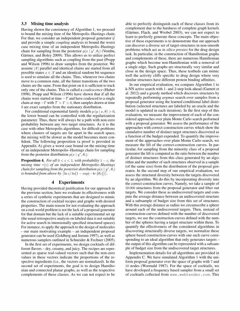
Figure 1: The figure shows the lift of correct-construction curves for considered graph and cocktail concepts. The lift indicateshow much more likely it is to see a target compared to the Monte Carlo search with a proposal generator.

Figure 2: The figure shows the dispersion of discovered targets relative to an algorithm with the identical proposal generator thatoutputs only targets. The reported curves can be seen as the percentage of discovered target class partitions given a budget.

sampler generates cocktail recipes by first sampling the num-ber of ingredients from the Poisson distribution and then itselects the recipe ingredients based on their co-occurrencefrequency in the collected data set. The parameters of thisproposal generator are moment-matched with respect to thecollected cocktail data set. As this proposal generator almostalways samples recipes with 2-10 ingredients, for n possibleingredients the number of different ingredient combinationsis∑10k=2

(nk

)(approximately n10). As the sampler is devel-

oped based on a set of cocktails with 335 ingredients thereare approximately 1024 different combinations of ingredientsin this search space. Thus, this is a huge search space thatcan provide an insight into the properties of the discoveryprocess on large scale problems. To label the cocktails gener-ated by this proposal generator we have trained decision treesfor each of the considered flavor profiles using a labeling ofthese cocktails according to flavor. All the reported resultswere obtained by averaging over 5 runs of the algorithm. TheMetropolis–Hastings sampling was performed with a burn-insample of 50 000 proposals and sampling was done for 50rounds/batches. In each round we take 10 i.i.d. samples byrunning 10 Metropolis–Hastings chains in parallel (note thatsamples from different rounds are dependent). To allow formodels of varying complexity, we have estimated the con-ditional exponential family regularization parameter in eachround using 5-fold stratified cross-validation. As the compet-ing approaches – argmax and k-NN active search (Garnett etal. 2012) – are not designed to search for targets without ana priori provided labeled structures, we have made a minormodification to our problem setting and warm-started eachmethod with a random sample of 5 target and the same num-

ber of non-target structures. For graphs these were chosenuniformly from the search space and for cocktails uniformlyfrom the available sample of cocktails. Note that without thiswarm-start the argmax search estimates the distribution oftarget structures with a single peak around the first discoveredtarget. Moreover, k-NN probabilistic model cannot learn aproperty until it sees more than k labeled structures and it isunlikely to observe a target in k successive samples from aproposal generator.

In Figure 3.3, we show the lift of the correct-constructioncurves for all the considered approaches. We have definedthese correct-construction curves by considering isomorphicgraphs and cocktails with equal sets of ingredients (ignoringportions of each ingredient) as identical structures. The plotsindicate that our approach and k-NN active search are able toemphasize the target class in all the domains for all the con-sidered properties. Moreover, for our approach the magnitudeof this emphasis is increasing over time and it is more likelyto generate a target as the process evolves. In all domainsand for all properties, k-NN active search discovers moretarget structures than our approach. For graph properties,we see that argmax search also discovers more targets thanour approach. For cocktails, argmax search discovers manycocktails with identical sets of ingredients and different por-tions of these (such cocktails are considered identical in thecorrect-construction curves). Thus, if we are only interestedin discovering target structures without considering structuraldiversity between them, our empirical evaluation indicatesthat it is better to use k-NN active search than Algorithm 1.

In Figure 3.3, we show the dispersion of target structuresdiscovered by each of the considered approaches. The plots

indicate that our approach achieves a large structural varietyof discovered targets. In all domains and for all properties, ourapproach outperforms both k-NN active and greedy argmaxsearch. These experiments also indicate that k-NN activesearch explores more than argmax search. In some of theplots, a dip can be observed in the curves for k-NN activeand argmax search. This can be explained by the exploitativenature of these algorithms and the fact that the search is fo-cused to a small region of the space until all the targets fromit are discovered. In contrast to this, our approach discoverstargets from the whole space and can cover a large numberof spheres centered at undiscovered samples with a relativelysmall number of targets. Thus, if we are interested in discov-ering diverse target structures, our results indicate that it isbetter to use Algorithm 1 than k-NN active or argmax search.

5 DiscussionActive search with k-NN probabilistic model (Garnett et al.2012) is a related approach with the problem setting similarto that of de novo design. The key distinction between theinvestigated problem setting and k-NN active search is in therequirement to discover structures from the whole domain.Garnett et al. (2012) assume that an extensional descriptionin the form of a finite subset of the domain is explicitlygiven as input to the algorithm. In this work we require onlyan intensional description of the domain. For instance, forthe domain of graphs on n ∈ N vertices, the intensional de-scription is just that of the number of vertices, while theextensional one consists of a list of all graphs on n vertices.In many cases, considering intensional descriptions is muchmore promising because an algorithm with an extensionaldescription of an exponentially large or uncountable searchspace can only consider small and often arbitrary subsetsof this space. The second key distinction between k-NN ac-tive search and de novo design is in the assessment of theiroutcomes. In particular, both approaches try to find, as soonas possible, as many as possible target structures. However,k-NN active search is designed to only discover members ofa target class and Algorithm 1 is designed to find membersof distinct structural partitions of a target class. This is veryuseful in domains where there are numerous isofunctionalstructures and in which k-NN active search outputs structuresfrom small number of structural partitions of a target class.

Recently, active search has been applied to a problemrelated to our cocktail construction task – interactive ex-ploration of patterns in a cocktail dataset (Paurat, Garnett,and Gartner 2014). The difference between our setting andthat of Paurat et al. (2014) is in the requirement to gener-ate novel and previously unseen cocktails exhibiting a targetproperty rather than searching for patterns in an existing cock-tail dataset. In addition to this, active search has been appliedto real-world problems where the search space is given bya single combinatorial graph, and some subset of its nodesis interesting (Wang, Garnett, and Schneider 2013). This isdifferent from applications we consider here and for whichthe search space is the space of all graphs of a given size.

As the investigated problem setting can be seen as a searchin structured spaces, our approach is, with certain distinctions,closely related to structured output prediction (Tsochantaridis

et al. 2004; Daume III, Langford, and Marcu 2009). In struc-tured output prediction the goal is to find a mapping froman instance space to a ‘structured’ output space. A commonapproach is to find a joint scoring function, from the space ofinput–output pairs to the set of reals, and to predict the outputstructure which maximizes the scoring function for each testinput. Finding a good scoring function can often be cast as aconvex optimization problem with exponentially many con-straints. It can be solved efficiently if the so-called separationand/or decoding sub-problems can be solved efficiently. Onedifference between the investigated setting and structured out-put prediction is in the assumption how input–output pairs arecreated. In particular, structured output prediction assumesthat the provided outputs are optimal for the given inputs. Inmany de novo design problems, it is infeasible to find the bestpossible output for a given input. For de novo drug designthis assumption implies that we would need to know the bestmolecule—from the space of all synthesizable molecules—with respect to different properties, such as binding affinityto specific protein sites. Moreover, as the decoding problemis designed assuming that the input–output pairs are optimalthe greedy argmax approach to solving this problem doesnot incorporate exploration. As a result of this, similar toargmax search these methods generate structures from a verysmall number of structural partitions of the target class. Otherdifferences are in the iterative nature of de novo design andin the hardness of the separation or decoding sub-problemsthat most structured output prediction approaches need tosolve. Another related sub-problem is that of finding preim-ages (Weston, Scholkopf, and Bakir 2004) which is typicallyalso hard in the context of structured domains except forsome special cases such as strings (Giguere et al. 2015).

Related to the proposed approach are also methods forinteractive learning and optimization as well as Bayesianoptimization. Interactive learning and optimization meth-ods implement a two-step iterative process in which anagent interacts with a user until a satisfactory solution is ob-tained. Some well-known interactive learning and optimiza-tion methods tackle problems in information retrieval (Yueand Joachims 2009; Shivaswamy and Joachims 2012) andreinforcement learning (Wilson, Fern, and Tadepalli 2012;Jain et al. 2013). However, these methods are only designedto construct a single output from the domain of real-valuedvectors and can not be directly applied to structured domains.Bayesian optimization (Brochu, Cora, and de Freitas 2010;Shahriari et al. 2015), on the other hand, is an approach to se-quential optimization of an expensive, black-box, real-valuedobjective. Rather than seeking a set of high-quality items,Bayesian optimization focuses on finding the single highest-scoring point in the domain. We, in contrast, consider discretelabels and wish to maximize the number of diverse targetsfound in an intensionally specified structured space. In drugdesign, this emphasis on exploring all parts of the searchspace is known as scaffold-hopping (Schneider and Fechner2005) and it is related to the problem of attrition (Schnei-der and Schneider 2016). Namely, in order to address thisproblem it is not sufficient to search for a molecule with thehighest activity level as it can be toxic or bind to an unde-sired protein in addition to the target protein. If attrition is

to be reduced an algorithm needs to find a number of struc-turally different molecules binding to a target protein. As ourapproach achieves a large structural variety of discoveredtargets, it has a potential to tackle this difficult problem.

AcknowledgmentsWe are grateful for access to the University of Nottingham High Per-formance Computing Facility. Part of this work was also supportedby the German Science Foundation (grant GA 1615/1-1).

ReferencesAkaike, H. 1973. Information theory and an extension of themaximum likelihood principle. In Second International Symposiumon Information Theory. Akademiai Kiado.Aldous, D. 1983. Random walks on finite groups and rapidly mixingMarkov chains. Seminaire de Probabilites XVII.Altun, Y.; Smola, A. J.; and Hofmann, T. 2004. Exponential familiesfor conditional random fields. In Proceedings of the 20th Conferenceon Uncertainty in Artificial Intelligence.Andrieu, C.; de Freitas, N.; Doucet, A.; and Jordan, M. I. 2003. Anintroduction to MCMC for machine learning. Machine Learning.Azuma, K. 1967. Weighted sums of certain dependent randomvariables. Tohoku Mathematical Journal.Bach, F. 2007. Active learning for misspecified generalized linearmodels. In Advances in Neural Information Processing Systems 19.Beygelzimer, A.; Dasgupta, S.; and Langford, J. 2009. Importanceweighted active learning. In Proceedings of the 26th InternationalConference on Machine Learning.Borgwardt, K. M. 2007. Graph kernels. Ph.D. Dissertation, LudwigMaximilians University Munich.Brochu, E.; Cora, V. M.; and de Freitas, N. 2010. A tutorial onBayesian optimization of expensive cost functions, with applicationto active user modeling and hierarchical reinforcement learning.arXiv preprint arXiv:1012.2599.Cameron, P. J. 1998. Introduction to Algebra. Oxford Univ. Press.Carl, B., and Stephani, I. 1990. Entropy, Compactness, and theApproximation of Operators. Cambridge University Press.Daume III, H.; Langford, J.; and Marcu, D. 2009. Search-basedstructured prediction. Machine Learning.Dixon, J. D., and Wilf, H. S. 1983. The random selection ofunlabeled graphs. Journal of Algorithms.Fine, S., and Scheinberg, K. 2002. Efficient SVM training using low-rank kernel representations. Journ. of Machine Learning Research.Garnett, R.; Krishnamurthy, Y.; Xiong, X.; Schneider, J.; and Mann,R. P. 2012. Bayesian optimal active search and surveying. In Pro-ceedings of the 29th International Conference on Machine Learning.Gartner, T.; Flach, P. A.; and Wrobel, S. 2003. On graph kernels:Hardness results and efficient alternatives. In Proceedings of the16th Annual Conference on Computational Learning Theory.Gelfand, I. M., and Fomin, S. V. 1963. Calculus of variations.Prentice-Hall Inc.Giguere, S.; Rolland, A.; Laviolette, F.; and Marchand, M. 2015.Algorithms for the hard pre-image problem of string kernels and thegeneral problem of string prediction. In Proceedings of the 32ndInternational Conference on Machine Learning.Goldberg, L. A., and Jerrum, M. 1997. Randomly samplingmolecules. In Proceedings of the 8th ACM SIAM Symposium onDiscrete Algorithms.

Guruswami, V. 2000. Rapidly mixing Markov chains: A comparisonof techniques (survey). Technical report, MIT.Huber, M. 1998. Exact sampling and approximate counting tech-niques. In Proceedings of the 30th Annual ACM Symposium on theTheory of Computing.Jain, A.; Wojcik, B.; Joachims, T.; and Saxena, A. 2013. Learningtrajectory preferences for manipulators via iterative improvement.In Advances in Neural Information Processing Systems 26.Jaynes, E. T. 1957. Information theory and statistical mechanics.Physical Review.Metropolis, N.; Rosenbluth, A. W.; Rosenbluth, M. N.; Teller, A. H.;and Teller, E. 1953. Equation of state calculations by fast computingmachines. The Journal of Chemical Physics.Paurat, D.; Garnett, R.; and Gartner, T. 2014. Interactive explorationof larger pattern collections: A case study on a cocktail dataset. InProceedings of KDD IDEA.Propp, J. G., and Wilson, D. B. 1996. Exact sampling with coupledMarkov chains and applications to statistical mechanics. In Proc. ofthe 7th International Conference on Random Struct. and Algorithms.Scannell, J. W.; Blanckley, A.; Boldon, H.; and Warrington, B. 2012.Diagnosing the decline in pharmaceutical R&D efficiency. NatureReviews Drug Discovery.Schneider, G., and Fechner, U. 2005. Computer-based de novodesign of drug-like molecules. Nature Reviews Drug Discovery.Schneider, P., and Schneider, G. 2016. De novo design at the edgeof chaos. Journal of Medicinal Chemistry.Shahriari, B.; Swersky, K.; Wang, Z.; Adams, R. P.; and de Freitas,N. 2015. Taking the human out of the loop: A review of Bayesianoptimization. Technical report, Universities of Harvard, Oxford,Toronto, and Google DeepMind.Shimodaira, H. 2000. Improving predictive inference under co-variate shift by weighting the log-likelihood function. Journal ofStatistical Planning and Inference.Shivaswamy, P., and Joachims, T. 2012. Online structured predictionvia coactive learning. In Proceedings of the 29th InternationalConference on Machine Learning.Tsochantaridis, I.; Hofmann, T.; Joachims, T.; and Altun, Y. 2004.SVM learning for interdependent and structured output spaces. InProc. of the 21st International Conference on Machine Learning.Vembu, S.; Gartner, T.; and Boley, M. 2009. Probabilistic structuredpredictors. In Proceedings of the 25th Conference on Uncertaintyin Artificial Intelligence.Wahba, G. 1990. Spline models for observational data. SIAM.Wang, X.; Garnett, R.; and Schneider, J. 2013. Active search ongraphs. In Proceedings of the 19th ACM SIGKDD InternationalConference on Knowledge Discovery and Data Mining.Weston, J.; Scholkopf, B.; and Bakir, G. H. 2004. Learning to findpre-images. In Adv. in Neural Information Processing Systems 16.White, H. 1982. Maximum likelihood estimation of misspecifiedmodels. Econometrica.Wilson, A.; Fern, A.; and Tadepalli, P. 2012. A Bayesian approachfor policy learning from trajectory preference queries. In Advancesin Neural Information Processing Systems 25.Woltosz, W. S. 2012. If we designed airplanes like we designdrugs... Journal of Computer-Aided Molecular Design.Wormald, N. C. 1987. Generating random unlabelled graphs. SIAMJournal on Computing.Yue, Y., and Joachims, T. 2009. Interactively optimizing informationretrieval systems as a dueling bandits problem. In Proceedings ofthe 26th International Conference on Machine Learning.

A ProofsProposition 1. Let P denote the set of all conditional distri-butions that have square integrable densities with respect toa base measure defined on the domain of a sufficient statisticφ (x, y) and support on the entire domain of φ (x, y). A max-entropy conditional distribution from P that satisfies a setof constraints on the first moments of the sample can be rep-resented as a conditional exponential model. To specify thisdistribution it is sufficient to find the maximum a posterioriestimator from the conditional exponential family of models.

Let f, g ∈ P and 〈f, g〉 =∫X×Y f (y | x) g (y | x) be the dot

product defined on this space. For a marginal distributionof structures p (x), the conditional entropy of a distributionp ∈ P is defined as

H (p | p) = −∫Xp (x)

∫Yp (y | x) ln p (y | x) .

Now, let φi denote the ith component of the feature mapφ. From the available sample it is possible to estimatethe empirical value of these component-statistics. In par-ticular, we can denote with αi = 1

n

∑nj=1 φi (xj , yj), where

(xj , yj) ∼ p0 (x, y). Then, a max-entropy distribution from Psatisfying a set of constraints on the first moments of thesample would be a solution of the following optimizationproblem

arg maxp∈P

H (p | p0)

s.t.∫X×Y

φi (x, y) p (y | x) p0 (x) ≤ αi, i ∈ I.

Proof. Gathering all the constraints and forming the La-grangian we get

L (p, λ) = −H (p | p0) +

∫Xλ (x)

(∫Yp (y | x)− 1

)+∫

X×Yλ (x, y) p (y | x) +

∑i∈I

λi

(∫X×Y

φi (x, y) p0 (x) p (y | x)− αi),

where λi ≥ 0 for all i ∈ I, λ (x) ≥ 0 for all x ∈ X , andλ (x, y) ≤ 0 for all x ∈ X and y ∈ Y.

For a functional F (p), the functional gradient ∇F at pis the principal linear term in the change of F after it isperturbed by ε in the direction of q (Gelfand and Fomin 1963,Section 3)

F (p+ εq) = F (p) + ε 〈∇F , q〉+O(ε2) .

Applying this derivation rule to the entropy term, we de-duce ∇pH = −p0 (x) (ln p (y | x) + 1). The functional gradi-ent of the Lagrangian is then given by

∇pL = p0 (x)

(1 + ln p (y | x) +

∑i∈I

λiφi (x, y)

)+

λ (x) + λ (x, y) .

Setting the functional gradient to zero, we obtain a max-entropy distribution satisfying the constraints,

p∗ (y | x) =exp (〈θ∗, φ (x, y)〉)

exp(λ∗(x)+λ∗(x,y)

p0(x)

) ,where φ = vec

(1, φii∈I

)and θ∗ = −vec

(1, λ∗i i∈I

).

As p (y | x) > 0 for all x ∈ X and all y ∈ Y , it follows fromthe complementary slackness that λ∗ (x, y) = 0. Now, takingλ∗ (x) = p0 (x) ln

∫Y exp (〈θ∗, φ (x, y)〉), we see that the max-

entropy conditional distribution is defined as

p∗ (y | x) =exp (〈θ∗, φ (x, y)〉)∫Y exp (〈θ∗, φ (x, y)〉)

.

Let us verify that this is indeed the desired distribution.For any other feasible conditional distribution r ∈ P we have

H (r | p0) = −∫X×Y

p0 (x) r (y | x) ln r (y | x)p∗ (y | x)

p∗ (y | x)≤

− KL (p∗, r)−∫X×Y

p0 (x) r (y | x) ln p∗ (y | x) ≤

−∫X×Y

p0 (x) r (y | x)

(−1− λ∗ (x)

p0 (x)−∑i∈I

λ∗i φi (x, y)

)≤

1 +

∫Xλ∗ (x) +

∑i∈I

λ∗iαi =

−∫X×Y

p0 (x) p∗ (y | x)

(−1− λ∗ (x)

p0 (x)−∑i∈I

λ∗i φi (x, y)

)=

−∫X×Y

p0 (x) p∗ (y | x) ln p∗ (y | x) = H (p∗ | p0) ,

where we have used the complementary slackness to trans-form the equation from line 4 to the one in line 5. In thesecond line, KL denotes the Kullback–Leibler divergence.

As already pointed out, the coefficients θ∗i i∈I are cho-sen to satisfy the moment constraints. Assuming thesecoefficients have been computed for the moment con-straints defined with equalities, the negative entropy ofp∗ (y | x) with respect to the empirical version of p0 (x),pemp0 (x) = 1

n

∑ni=1 1x=xi , is given by

−H (p∗ | pemp0 ) =1

n

n∑i=1

∫Yp∗ (y | xi) ln p∗ (y | xi) =

1

n

n∑i=1

∫Yp∗ (y | xi)

(〈φ (xi, y), θ∗〉 −A (θ∗ | xi)

)=

〈α, θ∗〉 − 1

n

n∑i=1

A (θ∗ | xi) =

1

n

n∑i=1

〈φ (xi, yi), θ∗〉 −A (θ∗ | xi) ,

where A (θ∗ | x) = ln∫Y exp

(〈φ (x, y), θ∗〉

). Thus, to find a

max entropy distribution it is sufficient to solve the followingnon-constrained convex optimization problem

θ∗ = arg maxθ

n∑i=1

〈φ (xi, yi), θ〉 −A (θ | xi) .

Setting the gradient of this objective function to zero, weverify that θ∗ satisfies the set of first moment constraintson the sample. Hence, the conditional exponential familymodel specified with the maximum a posteriori estimate ofthe parameter vector is a max entropy conditional modelsubject to constraints on the first moments of the sample.

Remark 1. We note here that Proposition 1 is just a minoradjustment of the classical result for exponential family mod-els (Jaynes 1957) and as such it should not be judged as acontribution of this paper.

Lemma A.1. For all 0 < ε < 1 and θ1, θ2 ∈ Θ such that‖θ1 − θ2‖ < 2pminε

r+√r2+2Λpminε

, it holds |L (θ1)− L (θ2)| < ε

and |L (θ1 | Dt)− L (θ2 | Dt)| < ε.

Proof. Performing the Taylor expansion of the log-likelihoodaround θ1 we get

ln p (y | x, θ2) ≤ ln p (y | x, θ1) +

Ey∼p(y|x,θ1)

[φ (x, y)> (θ2 − θ1)

]+

Λ

2‖θ2 − θ1‖2 .

Now, applying the Cauchy-Schwartz inequalityto the right hand-side and using the condition‖θ1 − θ2‖ < 2pminεΛ/r+

√r2+2Λpminε the claim follows,

i.e.,

|L (θ1)− L (θ2)| ≤ ‖θ1 − θ2‖(r +

Λ

2‖θ1 − θ2‖

)< ε,

|L (θ1 | Dt)− L (θ2 | Dt)| ≤‖θ1 − θ2‖

(r + Λ

2‖θ1 − θ2‖

)pmin

< ε.

Lemma A.2. Let ν = pminε/(2r+√

4r2+2Λpminε)

and letB1, . . . , BN (Θ,ν) be an ν-cover of the set Θ. Then

P

(supθ∈Θ|L (θ)− L (θ | Dt)| ≤ ε

)>

1−N (Θ, ν) sups=1,...,N (Θ,ν)

P(|L (θs)− L (θs | Dt)| >

ε

2

),

where θs denotes the center of the ball Bs.

Proof. From the assumptions of the lemma it follows thatsupθ∈Θ |L (θ)− L (θ | Dt)| > ε if and only if there exists1 ≤ s ≤ N (Θ, ν) such that supθ∈Bs

|L (θ)− L (θ | Dt)| > ε.Applying the union bound we get

P

(supθ∈Θ|L (θ)− L (θ | Dt)| > ε

)≤

N (Θ,ν)∑s=1

P

(supθ∈Bs

|L (θ)− L (θ | Dt)| > ε

).

(5)

On the other hand, we have

|L (θi)− L (θi | Dt)− L (θ) + L (θ | Dt)| <|L (θi)− L (θ)|+ |L (θi | Dt)− L (θ | Dt)| .

From the last equation and Lemma A.1 for θi center of Biand all θ ∈ Bi we get

|L (θ)− L (θ | Dt)| − |L (θi)− L (θi | Dt)| <ε

2.

As this holds for all 0 < ε < 1 and θ ∈ Bi weget that supθ∈Bi

|L (θ)− L (θ | Dt)| > ε implies|L (θi)− L (θi | Dt)| > ε

2. From here it follows that

P

(supθ∈Bs

|L (θ)− L (θ | Dt)| > ε

)<

P(|L (θs)− L (θs | Dt)| >

ε

2

).

(6)

Combining the results from Eq. (5) and (6) the claim follows.

Proposition A.3. (Carl and Stephani 1990) Let B be a finitedimensional Banach space and let BR be the ball of radiusR centered at the origin. Then, for d = dim(B), it holds

N (BR, ε, ‖·‖) ≤(

4R

ε

)d.

Theorem 2. Let p (y | x, θ) denote the conditional exponen-tial family distribution parameterized with a vector θ ∈ Θ,where Θ is a compact subset of a d dimensional Euclideanspace Rd. Let p0 (x, y) denote a latent data generating distri-bution such that, for all x ∈ X , the support of the likelihoodfunction p0 (y | x) is contained in the support of p (y | x, θ) forall θ ∈ Θ. Let

∣∣ln p (y | x, θ)∣∣ ≤ h (x, y) for all θ ∈ Θ and some

function h (x, y) : X × Y → R which is Lebesque integrablein the measure p0 (x, y). Then for all 0 < ε, δ < 1 there existsN (ε, δ) ∈ Ω

(1ε2

(d ln 1

ε+ ln 1

δ

))such that for all t ≥ N (ε, δ)

we have P(supθ∈Θ |L (θ)− L (θ | Dt)| ≤ ε

)≥ 1− δ.

According to our assumptions, the parameter set Θ is acompact subset of a finite dimensional Euclidean space andp (y | x, θ) is bounded away from zero for all x ∈ X , for ally ∈ Y, and for all θ ∈ Θ. Thus, we can assume that thereexists a constant pmin > 0 such that p (y | x, θ) ≥ pmin. LetΛ = maxθ∈Θ λ1 (θ), where λ1 denotes the largest eigenvalueof the Hessian matrix of the importance-weighted negativelog-likelihood objective function. As the set Θ is compactand the likelihood is a continuous function for all x ∈ X , theeigenvalues of the Hessian matrix are bounded. Therefore,there exists a finite maximizer Λ. From the compactness ofthe set Θ, it also follows there exists a finite ε-cover of this setfor all ε > 0. Before we proceed with the proofs, for the pur-pose of clarity, we review the notation introduced in Section 3.We denote with R > 0 the radius of a ball containing the set Θin its interior, i.e., ∀θ ∈ Θ it holds ‖θ‖ < R. Similarly, r > 0denotes the radius of a ball containing the mapped featuresin its interior, i.e., ∀x ∈ X , y ∈ Y it holds ‖φ (x, y)‖ < r.

Proof. We define all random variables with respect to a prob-ability space (Ω,D,P), where Ω is a state space, D is a σ-algebra of Ω, and P a probability measure of D. The samplingprocess is performed using an external source of randomnesswhich we model with an i.i.d. sequence of random variablesUtt∈N. We fix the filtration Dtt∈N where Dt ⊂ D is theσ-algebra generated by (U1, θ1, x1, y1) , . . . , (Ut, θt, xt, yt).

The input-output pair (xt+1, yt+1) is measurable with respectto the σ-algebra generated by (Dt, Ut+1). In other words,given the history of observations the pair is random only withrespect to Ut+1.

Having defined our random variables, we proceed withthe proof. In a part of the proof we use some of the standardtechniques from the theory of martingales and follow thesame principle as the proof of the importance weighted activelearning (Beygelzimer, Dasgupta, and Langford 2009). In thefirst step, we show that EDt [L (θ | Dt)] = L (θ). In particular,it holds

E [L (θ | Dt)] =1

t

t∑i=1

∫p0 (y∗)

p (y∗ | xi, θi)l (xi, yi, θ)P (Dt) =

1

t

t∑i=1

∫p0 (y∗)

p (y∗ | xi, θi)p (xi | y∗, θi) p0 (yi | xi) l (xi, yi, θ) ·

∫P (Dt−1 | xi, yi, θi)︸ ︷︷ ︸

=1

=1

t

t∑i=1

∫l (xi, yi, θ) p0 (xi, yi) =

L (θ) ,

where ` (x, y, θ) = A (θ | x)− 〈φ (x, y), θ〉.In the second step of the proof, we bound the discrepancy

between the empirical and the expected loss. As there is adependence within the sample, we cannot rely on the con-centration bounds requiring the independence assumption.Therefore, we introduce a sequence for which we prove it isa martingale and then proceed with bounding the discrepancyusing a martingale concentration inequality.

Let Wj , j = 1, . . . , t, be a sequence of random variablessuch that

Wj = −wj ln p (yj | xj , θ)− L (θ) , (7)

where wj =p0(y∗)

p(y∗|xj ,θj). According to the assumptions,

p (y | x, θ) is bounded away from zero for all x ∈ X ,for all y ∈ Y, and for all θ ∈ Θ. Thus, it holdssupθ∈Θ,x∈X ,y∈Y |ln p (y | x, θ)| < − ln pmin. From here it im-plies that |Wj | ≤ − ln pmin

pmin<∞ and E [|Wj |] <∞.

We now show that the sequence Zt =∑tj=0 Wj , with

W0 = 0, is a martingale. In particular,

E [Zt | Zt−1, . . . , Z0] =

Zt−1 + Ext,yt|Dt−1[wtl (xt, yt, θ)]− L (θ) = Zt−1.

On the other hand, it holds |Zt − Zt−1| = |Wt| ≤ − ln pminpmin

.From here using the inequality for martingales byAzuma (1967) we deduce

P(|L (θ | Dt)− L (θ)| > ε

2

)=

P

(|Zt| >

tε

2

)< 2 exp

(− tε2p2

min

8 (ln pmin)2

).

(8)

As this holds for all θ ∈ Θ, applying Lemma A.2 for

ν = pminε

2r+√

4r2+2Λpminεwe get

P

(supθ∈Θ|L (θ)− L (θ | Dt)| > ε

)<

2N

(Θ,

pminε

2r +√

4r2 + 2Λpminε

)exp

(− tε2p2

min

8 (ln pmin)2

).

From the last equation and Proposition A.3 we get

lnδ

2≥ d ln

4R(

2r +√

4r2 + 2Λpminε)

pminε− tε2p2

min

8 (ln pmin)2 =⇒

t

(pmin

ln pmin

)2

ε2 ∈ Ω

(d ln

1

ε+ ln

1

δ

)=⇒

t ∈ Ω

((ln pmin

pmin

)21

ε2

(d ln

1

ε+ ln

1

δ

))

Hence, we have shown that there exists a positive integerN ∈ Ω

(1ε2

(d ln 1

ε+ ln 1

δ

))such that for all 0 < ε, δ < 1, and

all t > N the claim holds.

Corollary 3. The sequence of estimators θtt≥1 convergesin probability to θ∗ ∈ Θ.

Proof. First note that from the compactness of Θ, it followsthat the Hessian of the negative log-likelihood is strictly posi-tive definite and, therefore, there exist unique minimizers ofthe loss functions L (θ) and L (θ | Dt). From Theorem 2, wehave that for sufficiently large twith probability 1− δ it holdsthat L (θ∗ | Dt) ≤ L (θ∗) + ε and L (θt) ≤ L (θt | Dt) + ε.From the strict convexity of the optimization objectiveL (· | Dt) it follows that L (θt | Dt) ≤ L (θ∗ | Dt). Hence, withprobability 1− δ

L (θt)− L (θ∗) ≤ |L (θt)− L (θt | Dt)|+L (θt | Dt)− L (θ∗ | Dt) + |L (θ∗ | Dt)− L (θ∗)| ≤ 2ε.

From here it follows that the sequence of estimators θtt≥0

converges in probability to the optimal parameter θ∗.

Definition A.1. Let M be a finite, ergodic Markov chaindefined on a state space Ω with transition probabilitiesp(x→ x′). A coupling is a joint process (A,B) = (At, Bt)on Ω× Ω such that each of processes A, B, consideredmarginally, is a faithful copy ofM.

Lemma A.4. (Aldous 1983) Let M be a finite, ergodicMarkov chain, and let (At, Bt) be a coupling for M. Sup-pose that P (At(ε) 6= Bt(ε)) ≤ ε, uniformly over the choice ofinitial state (A0, B0). Then the mixing time τ(ε) ofM (start-ing at any state) is bounded from above by t(ε).

Proposition 4. For all 0 < ε < 1, with probability 1− ε, themixing time τ(ε) of an independent Metropolis–Hastingschain for sampling from the posterior distribution p(x | y∗, θt)is bounded from above by

⌈ln ε/ ln

(1− exp(−4r ‖θt‖

)⌉.

Proof. As minx∈X p (y∗ | x, θt) ≤ maxx∈X p (y∗ | x, θt), thelower bound on the Metropolis–Hastings acceptance criterionis never greater than 1. Then, from Eq. (2) and (1) it followsthat, for a finite space Y, the transition probability from astate x to a state x′ satisfies

p(x→ x′) ≥exp(⟨φ(x′, y∗), θt

⟩−A(θt | x′)

)exp(⟨φ(x, y∗), θt

⟩−A(θt | x)

) =

∑y∈Y exp

(〈φ (x′, y∗) + φ (x, y) , θt〉

)∑y∈Y exp

(〈φ (x, y∗) + φ (x′, y) , θt〉

) .Now, we can lower bound the transition probability by

p(x→ x′) ≥|Y| exp

(2 · 〈φ (x↓, y↓) , θt〉

)|Y| exp

(2 · 〈φ (x↑, y↑) , θt〉

) ≥exp(−2 ·

∣∣⟨φ(x↓, y↓)− φ(x↑, y↑), θt⟩∣∣),

where 〈φ (x↓, y↓) , θt〉 and 〈φ (x↑, y↑) , θt〉 are the minimumand maximum values of the dot products appearing in thenumerator and denominator of p(x→ x′), respectively.

Then, using the Cauchy–Schwarz inequality, we derive

p(x→ x′) ≥ exp(−2∥∥φ(x↓, y↓)− φ(x↑, y↑)

∥∥‖θt‖).From our assumptions we have that ‖θ‖ ≤ R and‖φ(x, y)‖ ≤ r. Thus, it holds that

p(x→ x′) ≥ exp(−4r‖θt‖) ≥ exp(−4Rr). (9)

From Eq. (9) it follows that the probability of not coalescingfor T steps is upper bounded by

(1− exp(−4r‖θt‖)

)T . Thenfor t(ε) =

⌈ln ε/ ln

(1− exp(−4r‖θt‖)

)⌉, we have

P (At(ε) 6= Bt(ε)) ≤(1− exp(−4r‖θt‖)

)t(ε)= ε,

and from the coupling lemma (Aldous 1983; Guruswami2000, or see Lemma A.4/Definition A.1) we conclude that achain has mixed after t ≥ t(ε) steps with probability 1− ε.

Figure 3: The figure shows the lift of correct-construction curves for the considered concepts and their complements. The liftindicates that our approach is capable of emphasizing a target property, irrespective of its type – rare or dominant class.

Table 1: We report the fraction of target structures observed within 50 000 samples from the proposal generators. The samplingwas performed 5 times and the reported values are mean and standard deviation of the fractions computed over these runs.

GRAPHS, v = 7 GRAPHS, v = 10 COCKTAILS

HAMILTONIAN CONNECTED PLANAR HAMILTONIAN CONNECTED PLANAR DRY CREAMY JUICY

36.68% (±0.24) 65.01% (±0.20) 77.45% (±0.28) 8.68% (±0.15) 11.27% (±0.14) 16.83% (±0.14) 34.54% (±0.13)

B Additional plots

In this appendix, we present additional findings from oursynthetic experiments.

Emphasis of a target class. In Table 1, we give the distri-bution of the considered target classes and their complements.The table indicates that in our experiments we consider casesin which a target class is both rare and dominant. For graphconcepts, we consider the spaces of unlabelled graphs with 7and 10 vertices. The search space of graphs with 7 verticescontains only 1044 non-isomorphic graphs and it was usedfor sanity checks and tuning of our algorithm. The searchspace of graphs with 10 vertices, on the other hand, contains12 005 168 graphs and on this space for minority class proper-ties we have compared our approach to competing methods.The results of this comparison are presented in Section 4.Here, we present additional results indicating that our ap-proach is able to emphasize a target class property even incases when the property is dominant.

Similar to Section 4, to quantify the improvement ofour approach over the plain Monte Carlo search performedwith a proposal generator we measure the lift of its correct-construction curve. However, for sampling from the majorityclass the lift is defined as the ratio of the number of non-targets in a sample from the proposal generator and the num-ber of such structures generated by our approach. In otherwords, for dominant properties the lift quantifies how muchless likely it is to observe a non-target property when perform-ing the discovery using Algorithm 1 compared to the MonteCarlo search. In Figure 3, we show that Algorithm 1 is ableto emphasize the target classes in all domains, irrespective oftheir types – dominant or rare. Moreover, the magnitude ofthis emphasis is increasing over time and it is more likely todiscover a target as the process evolves.

Designed cocktails. In Table 2, for each of the three cock-tail property classes, we give five example cocktails con-structed by our algorithm at the termination of the experiment.The color of each ingredient indicates relative proportion inthe cocktail; more blue indicates a stronger presence. Theevaluation oracles used in these experiments are described inAppendix C.4. It is possible to compare the constructed cock-tail recipes to the real cocktails by looking up the displayedsets of ingredients at http://bartenderapp.com.

Table 2: Designed cocktailsDRY CREAMY JUICY

midori melon liqueur creme de cacao vodkajagermeister cream orange juicetequila bailey’s irish cream orange soda

gin bailey’s irish cream pineapple juicepowdered sugar green creme de menthe tequilanutmeg coffee blue curacaolemon heavy cream vodka

nutmeg

vodka gin sour mixtriple sec green creme de menthe lemon juicegrenadine creme de cacao tequila

scotch bailey’s irish cream ginjack daniels kahlua sweet and sourkahlua brandy orange juice

jagermeister milk cranberry juicemalibu rum kahlua peach schnapps

sugar

C Implementation detailsIn this appendix, we describe in details our experimental setup including the used proposal generators, kernel functions,and evaluation oracles. We first briefly review the competingapproaches and specifics of their implementations.

C.1 Competing methodsk-NN active search. One limitation of k-NN activesearch (Garnett et al. 2012) is the requirement that a finiteset of structures needs to be provided to the algorithm before-hand. In our experiments, we have simulated this approachwith 50 000 structures sampled from the proposal genera-tor and k-NN probabilistic model with k = 50 (ties are notpossible due to the choice of the hyperparameters).

In order to apply this approach to large sets of structureswith a different probabilistic model an efficient pruning strat-egy needs to be devised. In the original paper, the authorsgive the pruning rules only for k-NN probabilistic models.As it is non-trivial to come up with pruning rules for condi-tional exponential family models, a search with these modelswould be inefficient. For instance, for the investigated caseof Hamiltonian graphs with 10 vertices and an extensionaldescription in the form of a sample with less than 1% ofall structures from this space the active search with 2-steplook-ahead (Garnett et al. 2012) and a budget of 500 oracleevaluations requires more than 50 million parameter fittingsfor the search modeled with a conditional exponential family.

Argmax search. The argmax search works by taking a sam-ple of structures from a proposal generator and then choosinga structure from this sample with the highest conditionalprobability of it being a target. The selected structure is thenevaluated by the oracle and the conditional model is updatedto account for this new observation. This method is designedto compensate for the fact that k-NN active search with 1-steplook-ahead (Garnett et al. 2012) requires a finite sample ofstructures. For graphs, we use the uniform proposal gener-ator in combination with this strategy and this is the mostexploratory proposal generator for this greedy search strategy.The approach is simulated with the conditional exponentialfamily model, kernels and proposal generators identical tothe ones used by our approach.

C.2 Proposal generatorsA proposal generator is used to propose structures from anintensionally given domain. To be able to discover structureswith desired properties, the support of the proposal generatormust contain them. The uniform proposal generator is gener-ally a safe choice, as it guarantees that the entire space willeventually be discovered. In the absence of any other infor-mation about the desired structures, we advocate the uniformproposal generators from a maximum-entropy standpoint.However, when domain-specific knowledge is available, theproposal generator can be modified appropriately. This canbe especially useful when the class of structures with desiredproperties is relatively small compared to the entire searchspace, in which case the uniform proposal generator mightneed many samples to see a positive candidate.

We note here that while our theoretical results hold forproposal generators modeled with conditional Markov chains,we only demonstrate the potential of our approach in thesetting with uninformed samplers as proposal generators.The experiments with domain-specific conditional chains aredeferred to a journal version of the paper.

Sampling sparse vectors. Here, we describe a method forsampling sparse vectors based on a small set of examples.The small set of examples is there to serve as side knowledgefacilitating the design of a proposal generator. We use thismethod in Section 4 to propose cocktail recipes which arerepresented as sparse real-valued vectors.

In the first step, we ensure that the sampled construction isa sparse vector by setting the number of non-zero entries init. This is achieved by sampling the number of non-zero com-ponents from a Poisson distribution whose mean parameterwas obtained by moment-matching from data. This samplingprocess is repeated until we sample a number of non-zerocomponents greater than one.

In the second step, we sample components of the construc-tion and their values. In case we are interested in samplingonly binary vectors, than the value sampling part can beskipped. To choose the components of a construction weneed to make sure that components with high frequencyof appearance in data and combinations of frequently co-occurring components are selected more often. We achievethis by first building a component graph or an ingredient net-work in the case of cocktails with edges between the nodesweighted in accordance with the co-occurrence frequency.In addition to this, we keep a vector with the frequencies ofappearance of each component in the data. Then, the firstnon-zero component of a construction is chosen by samplingproportional to their appearance frequencies. Once the firstcomponent is sampled, we take its neighbors in the com-ponent graph and choose the next component by samplingproportional to the edge weights. Having sampled more thanone component, we create a candidate frequency vector bymerging the neighbor lists of the sampled components andaccumulating the edge weights of components with multipleoccurrences. In the last step of the process we sample thecomponent values. We perform this step by taking samplesfrom a triangular distribution. The mode and the value rangeparameters of these distributions are moment-matched fromdata (each component has a distribution).

We conclude the section with a formal descrip-tion of the sampling process. A construction repre-sented as a sparse vector is proposed with the fol-lowing sequence of steps: (i) m ∼ Poisson(η), (ii)c1 ∼ π (iii) ck ∼ τk =

∑k−1s=1 π

(cs) (2 ≤ k ≤ m), (iv)vk ∼ Triangular (uck , vck , µck ) (1 ≤ k ≤ m), where ckdenotes a non-zero component of the vector being sampled,τk the frequency vector such that the probability of samplinga component j is proportional to τkj , and vk is a valueassigned to the component ck. The parameters η, π, π(cs),uck , vck , and µck are moment-matched from data. In otherwords, given a data set with n sparse d-dimensional vectorswe do the following: (i) η = 1

n

∑ni=1 ni, where ni denotes

the number of non-zero components in the instance xi; (ii)

πj = 1n′∑ni=1 1xij 6=0, where xij denotes the component j

in the vector xi, πj its frequency of appearance in data,and n′ =

∑ni=1 ni; (iii) π(cs)

j = 1n′cs

∑i:xics 6=0 1xij 6=0, where

n′cs =∑i:xics 6=0 (ni − 1), j 6= cs, 1 ≤ j, cs ≤ d, π

(cs)cs = 0;

(iv) uj = max (0, µj − 2 ∗ σj), vj = min (1, µj + 2 ∗ σj), andµj and σj are the mean and the standard deviation of thecomponent j computed over the instances with non-zerovalues at this component. To enable the sampling of sparsevectors with combinations of non-zero components which arenot appearing together in data we do the Laplace smoothingof vectors π(cs) by adding 1/d to each of its components.

Sampling unlabelled graphs with n vertices. As the setof graphs is a complicated, combinatorial object, it can bedifficult to design an efficient uninformed sampler. In general,to sample a random unlabelled graph it is common to use theErdos–Renyi model with p = 1/2. This approach, however,samples some graphs too often and does not provide sufficientdiversity to the constructive process (e.g., the probabilityof sampling an unlabelled path with n vertices is n!

2times

higher than the probability of sampling the complete graphwith the same number of vertices). Instead, one could try tofirst sample the parameter p uniformly at random and then tosample a graph with edge probability p. The last method doesnot generate unlabelled graphs u.a.r., but it can be used toefficiently sample some graph concepts (e.g., acyclic graphs).In this paper we take the safest route and choose to proposegraphs with n vertices using the uniform sampler. We now doa review of this sampler for unlabelled graphs with n vertices.

Let Gn denote the set of all canonically labelled graphswith n vertices. A left action of a group S on a setX is a function µ : S ×X → X with the following twoproperties: (i) (∀x ∈ X)(∀s, t ∈ S) : µ(t, µ(s, x)) = µ(ts, x);(ii) (∀x ∈ X) : µ(e, x) = x (where e is the identity elementof the group S). If no confusion arises we write µ(s, x) = sx.A group action defines the equivalence relation ∼ on a set X,i.e., a ∼ b⇔ sa = b for some s ∈ S and a, b ∈ X. The equiv-alence classes determined by this relation are called orbitsof S in X. The number of orbits can be computed using theFrobenius–Burnside theorem (Cameron 1998).

Theorem C.1 (Frobenius–Burnside). Let X be a finite non-empty set and S be a finite group. If X is an S-set, then thenumber of orbits of S in X is equal to 1

|S|∑s∈S |Fix(s)| ,

where Fix(s) = x ∈ X | sx = x.

To sample unlabelled graphs uniformly at random,Wormald (1987) proposed a rejection sampling method basedon Theorem C.1. The idea is to consider the action of a sym-metric group Sn over the set Gn. Then, the orbits of Sn in theset Gn are non-isomorphic unlabelled graphs and to sampleunlabelled graphs uniformly it suffices to uniformly samplethe orbits (Dixon and Wilf 1983). Moreover, it is possible toshow (Dixon and Wilf 1983; Wormald 1987) that uniform or-bit sampling is equivalent to uniform sampling of an elementfrom the set Γ =

(π, g) | πg = g;π ∈ Sn, g ∈ Gn

.

According to Theorem C.1, an element (π, g) ∈ Γ can besampled u.a.r. by choosing a permutation π with probabil-ity proportional to |Fix(π)| and then choosing g ∈ Fix(π)u.a.r. Dixon & Wilf (1983) propose a more efficient

sampling algorithm by partitioning the symmetric groupinto conjugacy classes [πi] (1 ≤ i ≤ l) and sampling: (i)[πi] ∼ |[πi]||Fix(πi)|/on|Sn|, (ii) g ∈ Fix(πi) u.a.r.; where on de-notes the number of non-isomorphic unlabelled graphs andπi is a class representative for the class [πi]. As it holds|Fix(π)| = |Fix(π′)| and |Fix(π) ∩ [g]| = |Fix(π′) ∩ [g]| forπ, π′ ∈ [πi] then (Wormald 1987)

P([g])

=

l∑i=1

P([g], [πi]

)=

l∑i=1

P([πi])P([g] | [πi]

)=

l∑i=1

∣∣[πi]∣∣∣∣Fix(πi)∣∣

on|Sn|

∣∣Fix(πi) ∩ [g]∣∣∣∣Fix(πi)

∣∣ =1

on.

The problem with the approach is the fact that we needto know the exact number of non-isomorphic graphs withn vertices on to apply the algorithm and this number isnot computable in polynomial time. To overcome this,Wormald (1987) partitions the elements of the group Sn intoclasses [ck] = π ∈ Sn | support(π) = k, 0 ≤ k ≤ n, and up-per bounds

∣∣[ci]∣∣∣∣Fix(πi)∣∣ ≤ Bi. The algorithm then samples

an unlabelled graph u.a.r. as follows: (i) [ci] ∼ Bi/∑j Bj , (ii)πi ∈ [ci] u.a.r., (iii) g ∈ Fix(πi) u.a.r., and (iv) accept the sam-pled graph g with probability B−1

i

∣∣[ci]∣∣∣∣Fix(πi)∣∣; otherwise,

restart. On average, the method generates an unlabelled graphin time polynomial in the number of vertices.

C.3 Kernel functionsIn this section, we describe application-specific kernel func-tions used in Section 4. For these kernel functions, wefollow the standard procedure for tuple kernels and takekernels which factor into the product of domain kernels,k ((x, y) , (x′, y′)) = kX (x, x′)kY(y, y′), where kX and kY arekernel functions over spaces X and Y.

First we describe the property space kernel function kY .In all the cases considered in Section 4 the property spaceY is binary and we use the identity kernel. This is the spacerequiring the simplest feedback and the least effort froman evaluation oracle. In more complex experiments such asdrug design, the evaluation oracle could output a structuredlabel such as binary vector reflecting different aspects of theconstruction – price, binding properties, stability etc. In thesecases, one could take the property space Y to be the powerset of elementary properties and use the intersection kernelkY(yi, yj) = |yi ∩ yj |.

In the remainder of the section we describe the instancespace kernels for the investigated domains. To apply ouralgorithm to the space of graphs we use the random walkkernel (Gartner, Flach, and Wrobel 2003). The kernel per-forms random walks on both graphs and counts the numberof matching walks. It can be computed as

kX (G1, G2) =

|V×|∑i,j=1

∞∑n=0

[λnEn×]ij , (10)

where E× denotes the adjacency matrix of the product graphG1 ×G2 and λn is a sequence of hyperparameters thatneeds to be set such that the sum in (10) converges for any pairof graphs G1 and G2. We apply the kernel with λn = λn to

unlabelled graphs, and for this particular case E× = E1 ⊗ E2.The kernel can be computed efficiently using the fixed-pointmethod (Borgwardt 2007).

To apply our algorithm to the space of sparsereal-valued vectors, we use the Gaussian kernelwith diagonal relevance length scale matrix M , i.e.,kX (x, x′) = exp

(−1/2(x− x′)>M(x− x′)

). For each

coordinate we set the relevance scale as

mjj =2n√

nnz (maxni=1 xij −minni=1 xij),

where n denotes the number of instances, nnz the total num-ber of non-zero entries in the data set, d dimension of theinstances, and 1 ≤ j ≤ d.

C.4 Evaluation oraclesDRY

[1 | jagermeister ≥ 0.225 ? DRY : go to 2][2 | gin ≥ 0.465639 ? DRY : go to 3][3 | jackdaniels ≥ 0.138889 ? DRY : go to 4][4 | 151 proof rum ≥ 0.291666 ? DRY : go to 5][5 | vodka ≥ 0.437037 ? DRY : NOT DRY]

CREAMY[1 | bailey′s irish cream ≥ 0.03324 ? CREAMY : go to 2][2 | creme de cacao ≥ 0.0059365 ? CREAMY : go to 3][3 | milk ≥ 0.21495 ? CREAMY : go to 4][4 | irish cream ≥ 0.006375 ? CREAMY : go to 5][5 | cream ≥ 0.014754 ? CREAMY : NOT CREAMY]

JUICY[1 | orange juice ≥ 0.040152 ? JUICY : go to 2][2 | cranberry juice ≥ 0.084 ? JUICY : go to 3][3 | pineapple juice ≥ 0.183334 ? JUICY : go to 4][4 | sour mix ≥ 0.0625 ? JUICY : go to 5][5 | sweet and sour ≥ 0.274614 ? JUICY : NOT JUICY]