ACTIVE STABILIZATION OF ROTORCRAFT EXTERNAL SLUNG …

The Pennsylvania State University

The Graduate School

ACTIVE STABILIZATION OF ROTORCRAFT EXTERNAL

SLUNG LOADS IN HIGH SPEED FLIGHT USING AN ACTIVE

CARGO HOOK

A Thesis in

Aerospace Engineering

by

Zhouzhou Chen

© 2020 Zhouzhou Chen

Submitted in Partial Fulfillment

of the Requirements

for the Degree of

Master of Science

December 2020

ii

The thesis of Zhouzhou Chen was reviewed and approved by the following:

Joseph F. Horn

Professor of Aerospace Engineering

Thesis Co-Adviser

Jacob Enciu

Assistant Research Professor of Aerospace Engineering

Thesis Co-Adviser

Amy R. Pritchett

Professor of Aerospace Engineering

Head of the Department of Aerospace Engineering

iii

Abstract

For rotorcraft carrying slung loads, the stability is often a concern due to the complex slung

load dynamics when coupled to rotorcraft flying at high airspeeds. This thesis demonstrates active

stabilization of slung loads in high-speed flight by actuating the cargo hook. To show close

reference to future vertical lift configurations, the selected aircraft model is the generic tiltrotor

model developed by the US Army Technology Development Directorate (TDD). The slung load

is the M119 howitzer featured in many airdrop missions and rapid deployments. The dynamic

models of the load were identified using the frequency-response method for system identification.

The load was initially wind-tunnel tested at Tel Aviv University to collect flight data of the load

responses to cargo hook commands for a flight envelope from hover through 200 knots in full-

scale flight conditions. The wind tunnel test showed unstable load behavior at high airspeeds

reflected as Limit Cycle Oscillation (LCO) of the load pendulum motion within a certain speed

range. A set of linear models describing the slung load pendulum dynamics were identified using

system identification software CIFER® at airspeeds where the system was stable. An active cargo

hook (ACH) controller was designed using classical control methods to increase damping of the

load pendulum motions. A nonlinear rotorcraft-load-coupled model was developed in Simulink to

simulate the rotorcraft response due to the coupling effects from the load and to test the

performance of the designed ACH controller. The simulation results verified the controller

performance at increasing damping of the load pendulum motions and showed the effectiveness

iv

of the controller stabilizing the load in high-speed flight conditions. The simulation also showed

good agreement with the closed-loop wind tunnel test results.

v

Table of Contents

List of Figures vii

List of Tables xii

List of Symbols xiii

Acknowledgments xvii

Chapter 1 Introduction 1

1.1Motivation ...................................................................................................................1

1.2Background .................................................................................................................1

1.3 Objectives. .................................................................................................................3

Chapter 2 System Description and Modeling 7

2.1 Introduction ................................................................................................................7

2.2 External Load Model ..................................................................................................8

2.2.1 M119 Model Wind Tunnel Test ...........................................................................9

2.2.2 Identification of Slung Load Linear Models ....................................................... 16

2.3 Tiltrotor Model ......................................................................................................... 23

2.4 Coupled Tiltrotor-Load System. ............................................................................... 26

2.5 Linear Analysis of System Stability .......................................................................... 33

Chapter 3 Controller Design 41

3.1 Introduction .............................................................................................................. 41

3.2 Control Design for the Isolated Load ........................................................................ 42

3.4 Airspeed Scheduled Control Design for High-Speed Flight Conditions ..................... 52

3.5 GTR Stability Augmentation System (SAS) Control Design ..................................... 58

3.6 Control Design Conclusion ....................................................................................... 62

vi

Chapter 4 Simulation Results 63

4.1 Introduction .............................................................................................................. 63

4.2 Comparison with Closed-Loop Wind Tunnel Test .................................................... 64

4.3 GTR-Load Coupled System Simulation Results ........................................................ 70

4.3.1 Simulation at 120 knots ...................................................................................... 70

4.3.2 Simulation at 87 knots........................................................................................ 74

4.3.3 Simulation at hover ............................................................................................ 77

4.3 Simulation Results Conclusions ................................................................................ 79

Chapter 5 Conclusions and Future Work 80

5.1 Conclusions .............................................................................................................. 80

5.2 Future Work ............................................................................................................. 82

Bibliography 83

vii

List of Figures

Figure 1.1. Bell Boeing V-22 Osprey carrying an M119 Howitzer (downloaded from

https://www.alamy.com). .....................................................................................................4

Figure 1.2. Research Flowchart. ..................................................................................................5

Figure 2.1. M119 Howitzer model: (a) Folded configuration (b) Firing configuration (from [11]).9

Figure 2.2. M119 Howitzer model in the wind tunnel (from [14]).............................................. 11

Figure 2.3. Longitudinal and lateral cable angles (from [14]). .................................................... 12

Figure 2.4. Load attitude, cable angles, and hook force of the folded configuration during an

increase of the wind tunnel speed (from [14]). .................................................................... 14

Figure 2.5. Load attitude, cable angles, and hook force of the firing configuration during an

increase of the wind tunnel speed (from [14]). .................................................................... 15

Figure 2.6. (a): Longitudinal frequency sweep and cable angle response at zero wind tunnel speed

(firing configuration) (b): Frequency response of the longitudinal pendulum dynamics with

the fitted transfer function in CIFER. .............................................................................. 19

Figure 2.7. (a): Lateral frequency sweep and cable angle response at zero wind tunnel speed (firing

configuration). (b): Frequency response of the lateral pendulum dynamics with the fitted

transfer function in CIFER. ............................................................................................. 20

Figure 2.8. Generic tiltrotor rendering (from [9]). ...................................................................... 23

Figure 2.9. GTR Stitched model conversion corridor and linear model points. ........................... 26

viii

Figure 2.10. Schematic diagram of the tiltrotor-load coupled system. ........................................ 27

Figure 2.11. Coordinate systems of the tiltrotor-load coupled model. ........................................ 28

Figure 2.12. Bare-airframe low-frequency eigenvalues of the full-order model and 8-state model

(120 knots, 30° nac). .......................................................................................................... 35

Figure 2.13. Airspeed sweep of the bare-airframe low-frequency eigenvalues. .......................... 36

Figure 2.14. Low-frequency eigenvalues of the load-coupled model (120 knots, 30° nacelle angle,

firing configuration). .......................................................................................................... 38

Figure 2.15. Airspeed sweep of load-coupled model low-frequency eigenvalues (firing

configuration). .................................................................................................................... 39

Figure 2.16. Airspeed sweep of load-coupled model low-frequency eigenvalues (folded

configuration). .................................................................................................................... 40

Figure 3.1. Model of the open-loop system with active cargo hook and external slung load……...42

Figure 3.2. Open-loop simulation of lateral pendulum motion step response, (hover, firing

configuration). .................................................................................................................... 44

Figure 3.3. Block diagram of the closed-loop system. ................................................................ 45

Figure 3.4. Root locus plot of the lateral pendulum mode with lead compensation, (hover, firing

configuration). .................................................................................................................... 46

Figure 3.5. Broken-loop Bode diagram of the lateral pendulum mode with lead compensation,

(hover, firing configuration). .............................................................................................. 47

Figure 3.6. Closed-loop simulation of lateral pendulum motion step response with lead

compensation, (hover, firing configuration). ....................................................................... 48

Figure 3.7. Root locus plot of the lateral pendulum mode with lag compensation, (hover, firing

configuration). .................................................................................................................... 50

ix

Figure 3.8. Broken-loop Bode diagram of the lateral pendulum mode with lag compensation,


Figure 3.9. Closed-loop simulation of the lateral pendulum motion step response with lag and lead

compensation, (hover, firing configuration). ....................................................................... 52

Figure 3.10. Closed-loop simulation of the lateral pendulum motion step response with lag

compensation, (multiple airspeeds, firing configuration)..................................................... 53

Figure 3.11. Root locus plot of the longitudinal pendulum mode with lag compensation, (hover,

firing configuration). .......................................................................................................... 54

Figure 3.12. Broken-loop Bode diagram of the longitudinal pendulum mode with lag compensation,


Figure 3.13. Closed-loop simulation of the lateral pendulum motion step response with time delay,


Figure 3.14. Eigenvalues of the load-coupled model (firing configuration) with the SAS controller:

(a) Hover, (b) 120 knots, 30° nacelle angle. ........................................................................ 61

Figure 4.1. (a): Closed-loop system load response to increasing wind-tunnel speed with the ACH

controller (folded configuration) (from [19]). (b): Open-loop system load response to

increasing wind-tunnel speed without the ACH controller (folded configuration) (from [14]).

........................................................................................................................................... 65

Figure 4.2. (a): Closed-loop system load response to increasing wind-tunnel speed with the ACH

controller (firing configuration) (from [14]). (b): Open-loop system load response to

increasing wind-tunnel speed without the ACH controller (firing configuration) (from [14]).

........................................................................................................................................... 66

x

Figure 4.3. Comparison between the closed-loop wind-tunnel test and the simulation results at

14m/s (122 knots full-scale) with longitudinal hook excitation (firing configuration). ........ 68

Figure 4.4. Comparison between the closed-loop wind-tunnel test and the simulation results at

14m/s (122 knots full-scale) with lateral hook excitation (firing configuration). ................. 69

Figure 4.5. Tiltrotor attitude angle response to a 30% lateral doublet input at 120 knots, 30° nacelle

angle. ................................................................................................................................. 71

Figure 4.6. Load cable angle response to a 30% lateral doublet input at 120 knots, 30° nacelle

angle. ................................................................................................................................. 72

Figure 4.7. Cargo hook control action to a 30% lateral doublet input at 120 knots, 30° nacelle angle.

........................................................................................................................................... 73

Figure 4.8. Load cable angle response and cargo hook control action with a gain-reduced controller.

........................................................................................................................................... 73


angle. ................................................................................................................................. 75


angle. ................................................................................................................................. 76


........................................................................................................................................... 76


angle. ................................................................................................................................. 77

Figure 4.13. Load cable angle response to a 30% lateral doublet input at 5 knots, 90° nacelle angle.

........................................................................................................................................... 78

xi


........................................................................................................................................... 78

xii

List of Tables

Table 2.1. Froude scaling. ......................................................................................................... 10

Table 2.2. Frequency sweep test parameters (from [14]). ........................................................... 17

Table 2.3. Identified pendulum models for the firing configuration (from [14]). ........................ 22

Table 2.4. Identified pendulum models for the folded configuration (from [14]). ....................... 22

Table 2.5. Tiltrotor Configuration Data (from [9]). .................................................................... 24

Table 2.6. Eigenvalues of the GTR stitched model (120 knots, 30° nacelle angle). .................... 35

Table 2.7. Eigenvalues of the stitched model and load coupled model (120 knots, 30° nacelle

angle)………………………………………………………………………………………..38

Table 3.1. Controller parameters for the lateral pendulum mode (hover, firing configuration)…...45

Table 3.2. Preliminary ACH controller parameters. ................................................................... 56

Table 3. 3. System stability margins in the firing configuration. ................................................ 56

Table 3.4. System stability margins in the folded configuration. ................................................ 56

xiii

List of Symbols

Variables

𝐴, 𝐵, 𝐶, 𝐷 State matrix, input matrix, output matrix, feedthrough matrix

𝑎 Acceleration magnitude

𝛽0, 𝛽1𝑐 , 𝛽1𝑠 , 𝛽2 Rotor flapping angles

C(s) Compensator transfer function

d Lag compensator frequency

𝛿𝑥 , 𝛿𝑦 Commanded lateral and longitudinal cargo hook actuation

𝛿𝑎 , 𝛿𝑒, 𝛿𝑟 Aileron, Elevator, Rudder inputs

𝛿𝑛𝑎𝑐 Symmetrical nacelle angle

Δ𝜃0, Δ𝜃1𝑐′, Δ𝜃1𝑠

′ Differential collective, phased lateral cyclic, phased

longitudinal cyclic

𝐹 Force magnitude

G(s) Filter transfer function

𝐾 ACH controller gain

𝐾𝑃 , 𝜁𝑝, 𝜔𝑃 Transfer function parameters (gain, damping, and natural

frequency)

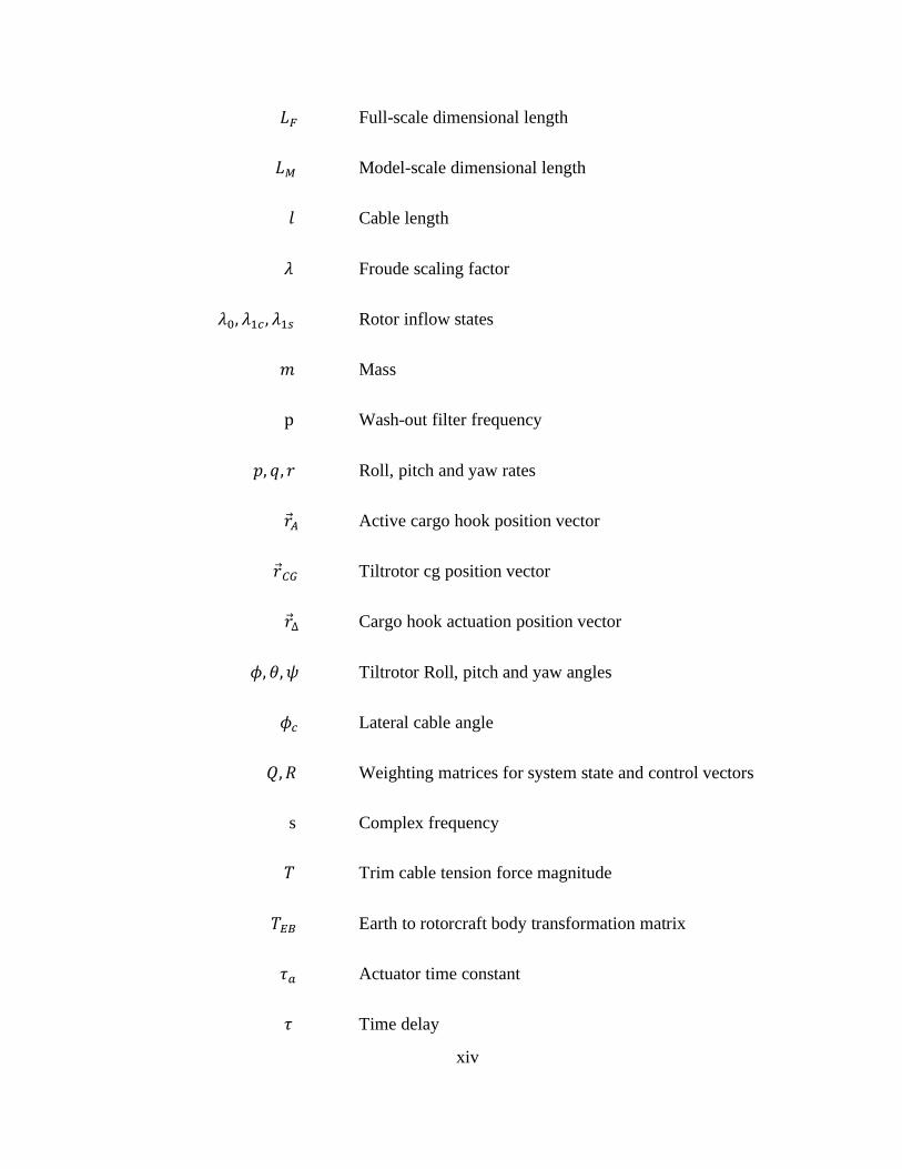
xiv

𝐿𝐹 Full-scale dimensional length

𝐿𝑀 Model-scale dimensional length

𝑙 Cable length

𝜆 Froude scaling factor

𝜆0, 𝜆1𝑐 , 𝜆1𝑠 Rotor inflow states

𝑚 Mass

p Wash-out filter frequency

𝑝, 𝑞, 𝑟 Roll, pitch and yaw rates

𝑟𝐴 Active cargo hook position vector

𝑟𝐶𝐺 Tiltrotor cg position vector

𝑟∆ Cargo hook actuation position vector

𝜙, 𝜃, 𝜓 Tiltrotor Roll, pitch and yaw angles

𝜙𝑐 Lateral cable angle

𝑄, 𝑅 Weighting matrices for system state and control vectors

s Complex frequency

𝑇 Trim cable tension force magnitude

𝑇𝐸𝐵 Earth to rotorcraft body transformation matrix

𝜏𝑎 Actuator time constant

𝜏 Time delay

xv

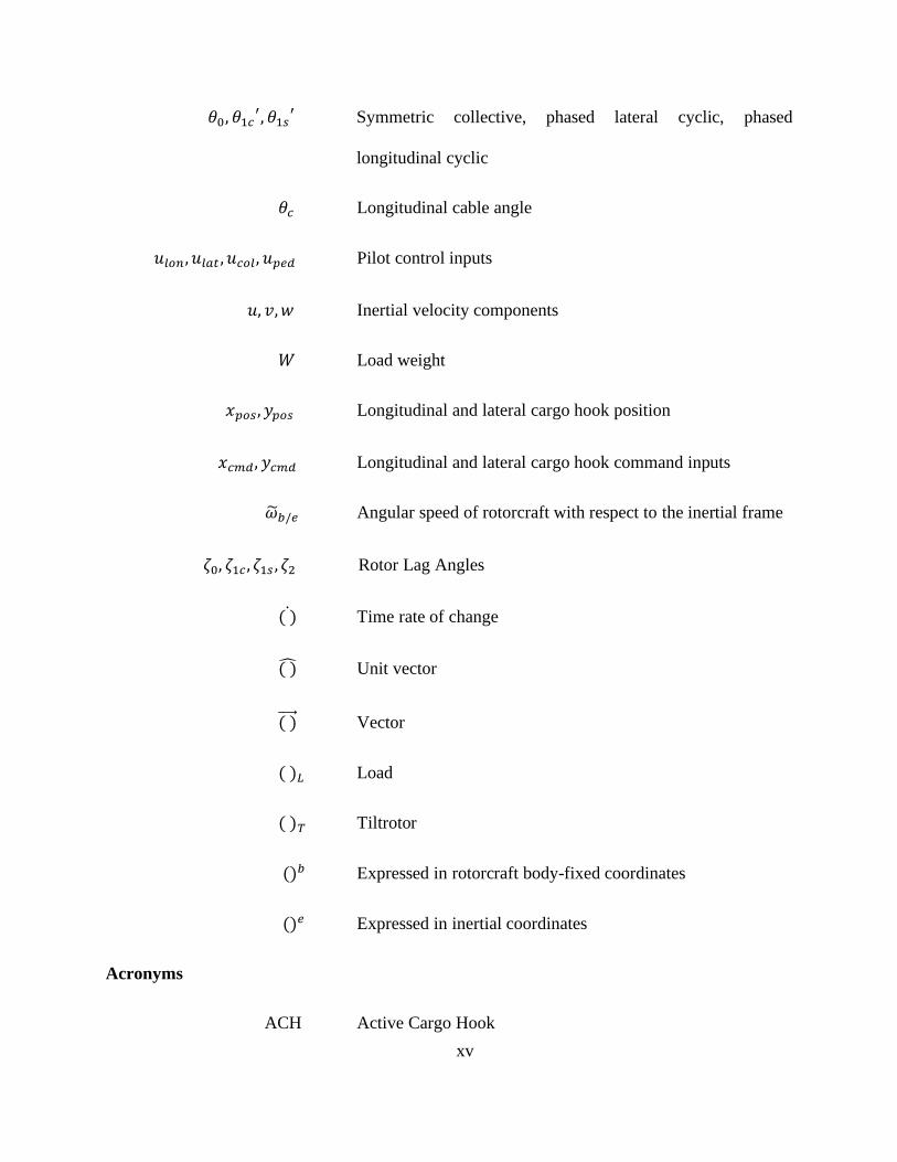
𝜃0, 𝜃1𝑐′, 𝜃1𝑠

′ Symmetric collective, phased lateral cyclic, phased

longitudinal cyclic

𝜃𝑐 Longitudinal cable angle

𝑢𝑙𝑜𝑛 , 𝑢𝑙𝑎𝑡 , 𝑢𝑐𝑜𝑙, 𝑢𝑝𝑒𝑑 Pilot control inputs

𝑢, 𝑣, 𝑤 Inertial velocity components

𝑊 Load weight

𝑥𝑝𝑜𝑠 , 𝑦𝑝𝑜𝑠 Longitudinal and lateral cargo hook position

𝑥𝑐𝑚𝑑, 𝑦𝑐𝑚𝑑 Longitudinal and lateral cargo hook command inputs

��𝑏/𝑒 Angular speed of rotorcraft with respect to the inertial frame

𝜁0, 𝜁1𝑐 , 𝜁1𝑠 , 𝜁2 Rotor Lag Angles

( ) Time rate of change

( ) Unit vector

( ) Vector

( )𝐿 Load

( )𝑇 Tiltrotor

()𝑏 Expressed in rotorcraft body-fixed coordinates

()𝑒 Expressed in inertial coordinates

Acronyms

ACH Active Cargo Hook

xvi

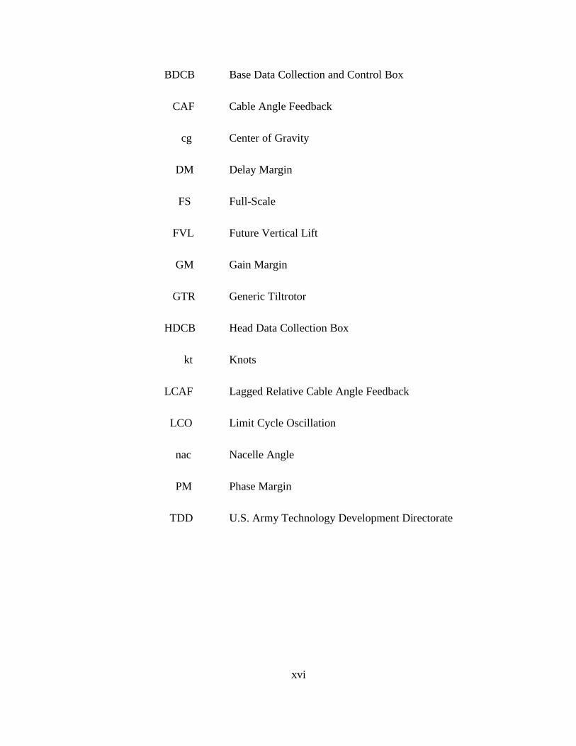
BDCB Base Data Collection and Control Box

CAF Cable Angle Feedback

cg Center of Gravity

DM Delay Margin

FS Full-Scale

FVL Future Vertical Lift

GM Gain Margin

GTR Generic Tiltrotor

HDCB Head Data Collection Box

kt Knots

LCAF Lagged Relative Cable Angle Feedback

LCO Limit Cycle Oscillation

nac Nacelle Angle

PM Phase Margin

TDD U.S. Army Technology Development Directorate

xvii

Acknowledgments

Firstly, I would like to thank Dr. Joseph Horn and Dr. Jacob Enciu for the help and guidance they

have provided me throughout the past two years. I truly appreciate Dr. Horn for giving me this

great opportunity to conduct research in the Vertical Lift Research Center of Excellence (VLRCOE)

and to work on this project. I have gained many knowledge and experience being alongside Dr.

Horn and working under his instructions. I would also want to acknowledge the work and efforts

that Dr. Enciu has contributed to this project. Through countless meetings and discussions, Dr.

Enciu has given me invaluable help on this project and many important advice. It won’t be possible

to achieve the current phase of the project without him.

Secondly, I would like to thank all the researchers including Reuben Raz, Aviv Rosen, Samuel

Nadell, and Luigi Cicolani that have performed the fundamental works for this project. Their

efforts have made it possible for me to focus on my part of the research and having confidence in

the results.

Finally, I want to thank my family for giving me support and care throughout the years. They have

never stopped encouraging me and building my confidence even though we are apart from each

other.

This research was partially funded by the Government under Agreement No. W911W6-17-2-0003.

The U.S. Government is authorized to reproduce and distribute reprints for Government purposes

not withstanding any copyright notation thereon. The views and conclusions contained in this

xviii

document are those of the authors and should not be interpreted as representing the official policies,

either expressed or implied, of the Aviation Development Directorate or the U.S. Government.

1

Chapter 1 Introduction

1.1 Motivation

External slung load carriage has been studied and discussed frequently for various applications

of rotorcraft transport of large loads such as civil construction, military combat, logging, and

firefighting work. For rotorcraft slung load missions, the dynamics of the load and the aircraft are

important attributes for the overall safety and maneuverability of the flight system. In forward

flight, rotorcraft carrying slung loads frequently encounter drastic or unstable load motion that

requires a restriction on the operational envelope of the rotorcraft. The speed of the rotorcraft is

largely limited when carrying a slung load in consideration of the safety of the flight and the

workload on the pilot. With load stabilization, the vehicle can usually fly faster with less demand

from the pilot input. As Future Vertical Lift rotorcrafts are designed to operate at airspeeds over

200 knots including the requirement for high-speed carriage of slung loads, it is important to

develop a methodology to stabilize the load across an operational envelope with a higher speed

limit.

1.2 Background

Past studies have shown load stabilization methods in passive or active manners. For passive

stabilization, methods such as using customized rigging or employing stabilizing add-ons can both

extend the flight envelope of the load. In Ref [1], rigid and fabric fins were installed on the back

of a CONEX box carried by a UH-60 rotorcraft to provide directional stability. Ref [2] used active

rotation with controlled anemometric cups to suppress the load pendulum motions. Both methods

2

can extend the operational limit of the system from 60 knots to over 100 knots. However, while

passive stabilization methods are easy to implement, it usually requires customization for different

types of load. The additional weight and drag caused by the add-ons can degrade the performance

and handling qualities of the rotorcraft.

For active stabilization, the load motion can be stabilized by the motion of the rotorcraft when

providing the correct control algorithm or by an active device designated specifically for the slung

load. In Ref [3], a control system was developed that uses Cable Angle Feedback (CAF) as well

as conventional fuselage feedback to improve load damping and handling qualities for hover/low-

speed operations. This control system was designated for a UH-60 platform and the effectiveness

of the system was demonstrated in a piloted fixed-base simulation. In Ref [4], Krishnamurthi and

Horn introduced lagged cable angle feedback (LCAF), which eliminates noisy cable angle and rate

sensor signals. The designed controller with LCAF was shown effective at reducing load

oscillations at hover/low speed with trade-offs in pilot response. Using active stabilization can also

be applied in the area of precision handling of the load. In Ref [5], an active controller was designed

and integrated with the primary flight control system that allows a UAV helicopter to safely

transport a slung load and to place it precisely on a moving platform such as a truck or a ship.

Another type of technique was developed by the Boeing Company that uses an active

stabilization device called the active cargo hook (ACH). The active cargo hook automatically

varies the hook position where the slung load is attached to and stabilizes the load without the

requirement for pilot intervention. Such technique was flight-tested on an H-6 flying testbed where

the cargo hook was moved longitudinally and laterally based on LCAF [6]. The test results showed

a significant increase in load damping and reduction of pilot workload during low-speed flight. In

Ref [7], the stabilization method of using ACH with LCAF was further investigated across the

3

flight envelope of a UH-60 helicopter with a focus on the higher speed range. Simulations of the

rotorcraft/load coupled system showed that the controller was successful in providing system

stability throughout the target flight speed envelope from hover to 100 knots.

Based on the results mentioned above, a research program for the development of active

stabilization methods of external loads during high-speed flights was recently initiated by the

Combat Capabilities Development Command (CCDC) and U.S. Army Technology Development

(TDD). The project aims to expand the flight envelope of slung-load carriage missions and

investigate the feasibility of using both CAF to the rotorcraft primary flight control system and the

ACH for load stabilization during highspeed flights. The application of ACH will be discussed in

this thesis.

1.3 Objectives.

The objective of this thesis is to present a thorough study of the slung-load system that

incorporates an FVL tiltrotor model and an M119 howitzer load model. The study focuses on the

application of ACH stabilization of the load during highspeed flights and applies both wind-tunnel

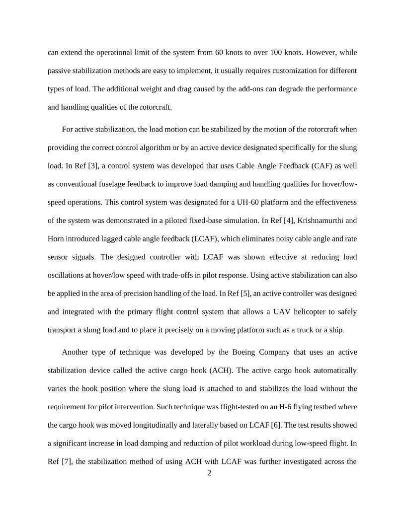
testing and dynamic simulations to investigate the performance of the ACH. Figure 1.1 shows a

V-22 Osprey as an example of the FVL tiltrotor.

4

Figure 1.1. Bell Boeing V-22 Osprey carrying an M119 Howitzer (downloaded from

https://www.alamy.com).

The research contains the joint effort between organizations from Israel and the U.S and is

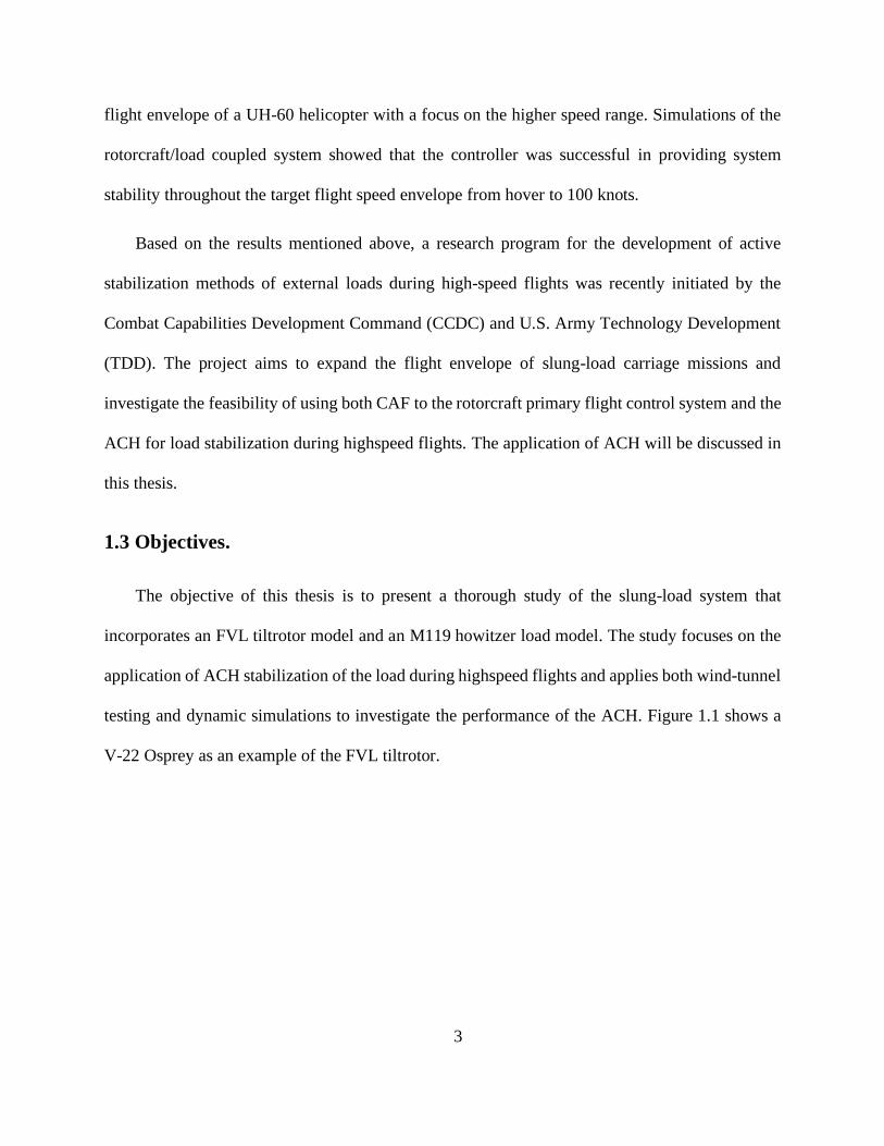
conducted under the Rotorcraft Project Agreement (RPA) between the two. Figure 1.2 shows a

simplified flowchart of the research. The Israeli researchers first performed the open-loop wind

tunnel tests across the flight envelope from zero to 23 m/s (equivalent to 200 knots in full-scale

condition). During the tests, multiple cargo hook inputs were tested to expose the dynamics of the

load throughout a range of speed of interest. Frequency-sweep inputs were utilized to generate

frequency response of the load pendulum dynamics. Researchers at TDD conducted system

identifications based on the results from the wind tunnel tests to provide linear models of the load

pendulum dynamics at different airspeeds.

5

After the initial wind-tunnel tests and system identifications, a preliminary control design

based on the load linear models was conducted. The controller was designed to use CAF as the

inputs and calculate the corresponding hook motion to stabilize the load pendulum motions. The

load was later integrated with the FVL tiltrotor in Simulink to perform simulations of the coupled

load/rotorcraft model as well as to conduct linear analysis accessing the stability of the coupled

system. The performance of the controller was validated from the simulation results and the closed-

loop wind-tunnel tests.

Figure 1.2. Research Flowchart.

The work in this thesis is organized as described in the following. In Chapter 2, the

development of the coupled load/aircraft model is presented. The first part of this chapter

summarizes the fundamental work performed by the other organizations, which includes the open-

6

loop wind-tunnel tests conducted by the Israeli researchers and system identification conducted by

TDD. The second part of the chapter presents the generic tiltrotor model (GTR) developed by TDD.

A detailed description of the coupling procedure of the load and the tiltrotor model is shown after

the introduction of the rotorcraft. At the end of the chapter, the stability analysis of the low-

frequency dynamics of the coupled system is discussed. In Chapter 3, the preliminary controller

design for the isolated load is demonstrated. The design process compares two ACH controllers

using lead and lag compensations to stabilize the load and also shows a detailed analysis of the

performance of the controllers in terms of damping ratio, stability margins, and resulting cargo

hook usage for control action. In Chapter 4, the closed-loop wind tunnel results are compared with

the simulation results. The coupled system was simulated at different airspeeds with the same sets

of command inputs as the closed-loop wind-tunnel experiment to check the accuracy of the

simulation model. The simulation results including responses of the tiltrotor and load and the

actuation of the cargo hook are plotted for better visualization of the system dynamics. Chapter 5

summarizes the studies of the M119 slung load and coupled tiltrotor/load system and suggests the

future work that could be done to improve the performance of the ACH controller.

7

Chapter 2 System Description and Modeling

2.1 Introduction

This section will describe the development of the M119 Howitzer slung load model.

Researchers at Technion University designed and conducted wind-tunnel experiments to a scaled

model of the M119 load. The wind-tunnel experiment featured a newly designed hardware-in-the-

loop (HIL) setup that incorporates a moving cargo hook, multiple sensors for data measurements,

and a computer for data processing. Initial open-loop tests were performed by placing the load

model in an airspeed-increasing wind field. The response of the load motion was recorded along

with the airspeed to evaluate the dynamic stability of the load model across the flight envelope.

Frequency sweep tests were performed after the open-loop tests to identify dynamic load models.

The load was excited by the moving cargo hook at varying frequency and the resulted cable angles

were recorded to generate frequency response of the load pendulum motions to the hook command.

The definition of cable angles will be explained in later sections. The tests were repeated at

different airspeeds where the load was dynamically stable. The linear models of the load pendulum

motions were then identified by TDD through the frequency response at each test speeds.

The aircraft model used in the study was a generic tilt rotor model developed by the TDD

that has a flight envelope from hover to 260 knots. The model was constructed based on 228 linear

models at different flight conditions, which were extracted from a nonlinear flight dynamics model

developed using HeliUM [9]. Model stitching technique was applied during the development of

8

the simulation model that combined a collection of linear state-space models for discrete flight

conditions, with corresponding trim data, into one continuous, full-envelope flight-dynamics

simulation model [10].

At later stages, model coupling was conducted to the slung load model and the tiltrotor

model to analyze the interactions between the different dynamics from the two models and study

the effects of the slung load on the aircraft across the flight envelope.

2.2 External Load Model

The M119 Howitzer is a lightweight 105mm gun used by the United States Army, it is

frequently transported by rotorcraft on the combat field. An M119 howitzer gun weighs 4400 lb

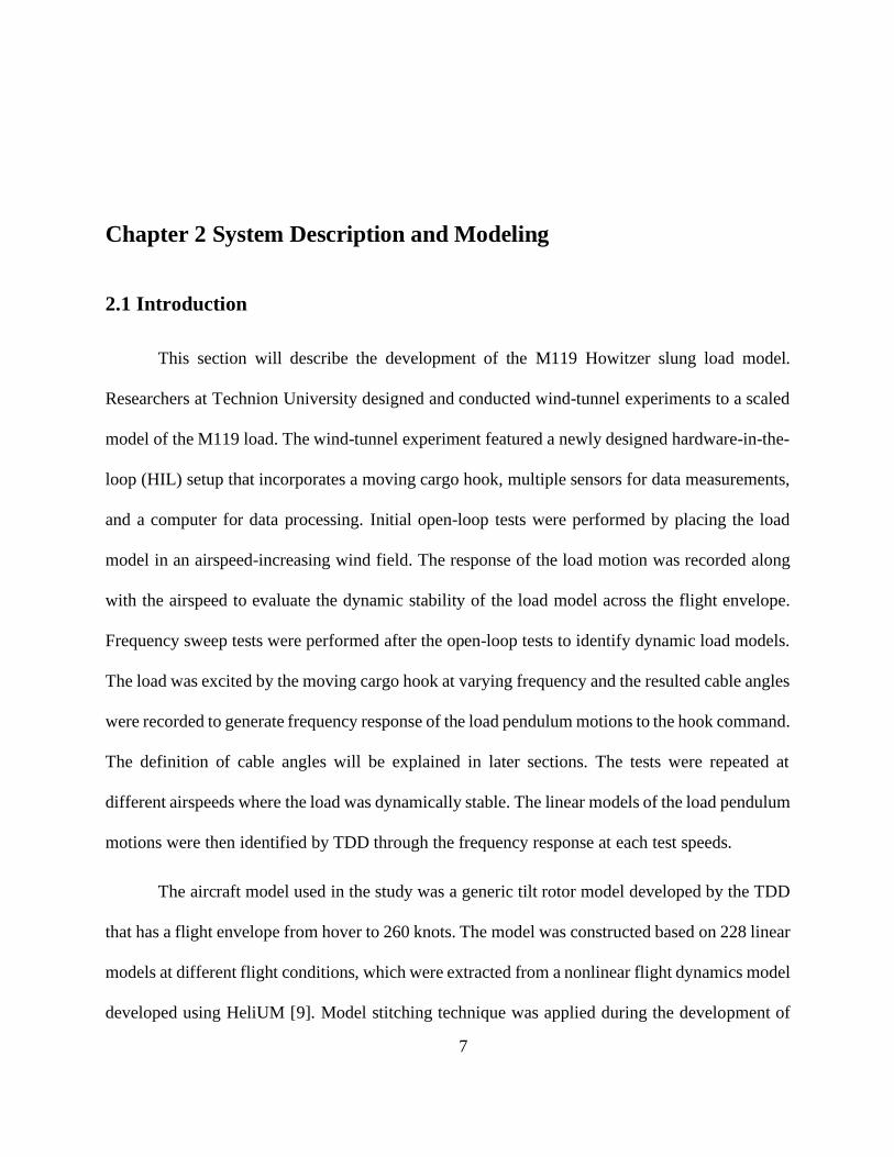
[11] and has two configurations during transportation. Figure 2.1(a) shows the howitzer being

carried in the folded position such that the gun barrel is folded into the firing platform and figure

(b) shows the firing configuration with the barrel fully extended.

(a)

9

(b)

Figure 2.1. M119 Howitzer model: (a) Folded configuration (b) Firing configuration (from

[11]).

2.2.1 M119 Model Wind Tunnel Test

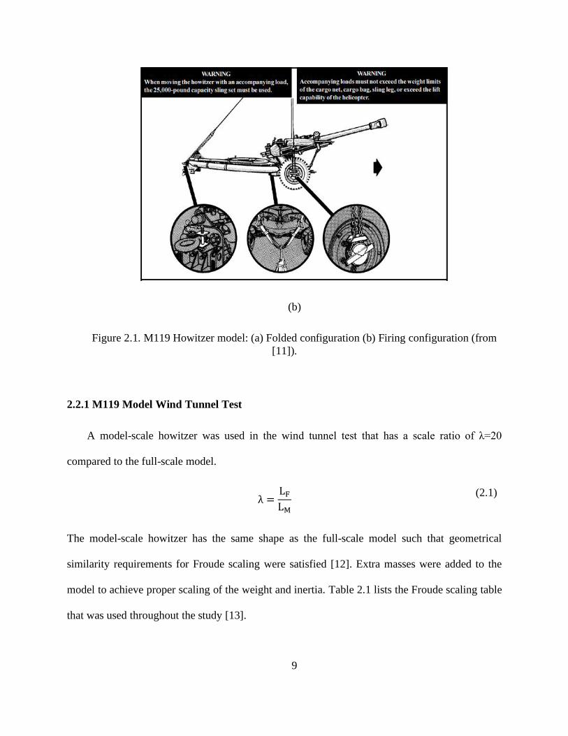
A model-scale howitzer was used in the wind tunnel test that has a scale ratio of λ=20

compared to the full-scale model.

λ =

LF

LM

(2.1)

The model-scale howitzer has the same shape as the full-scale model such that geometrical

similarity requirements for Froude scaling were satisfied [12]. Extra masses were added to the

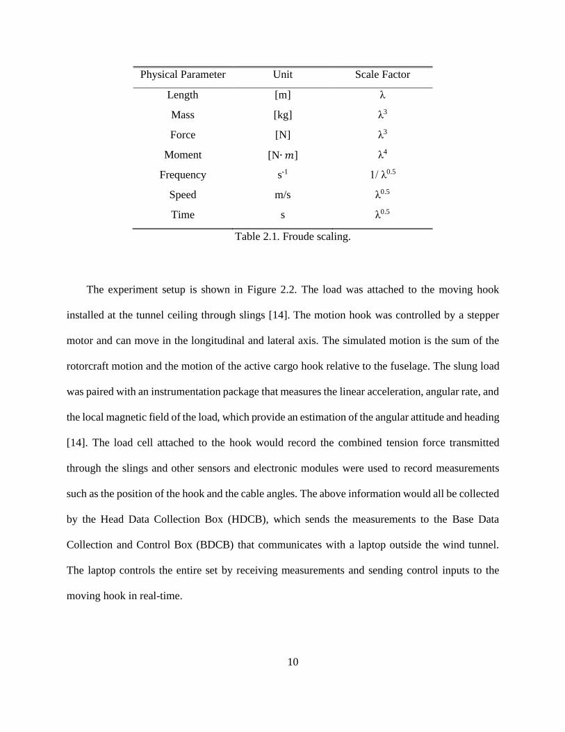
model to achieve proper scaling of the weight and inertia. Table 2.1 lists the Froude scaling table

that was used throughout the study [13].

10

Physical Parameter Unit Scale Factor

Length [m] λ

Mass [kg] λ3

Force [N] λ3

Moment [N∙ 𝑚] λ4

Frequency s-1 1/ λ0.5

Speed m/s λ0.5

Time s λ0.5

Table 2.1. Froude scaling.

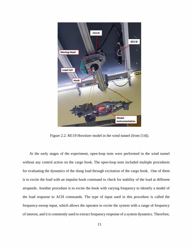
The experiment setup is shown in Figure 2.2. The load was attached to the moving hook

installed at the tunnel ceiling through slings [14]. The motion hook was controlled by a stepper

motor and can move in the longitudinal and lateral axis. The simulated motion is the sum of the

rotorcraft motion and the motion of the active cargo hook relative to the fuselage. The slung load

was paired with an instrumentation package that measures the linear acceleration, angular rate, and

the local magnetic field of the load, which provide an estimation of the angular attitude and heading

[14]. The load cell attached to the hook would record the combined tension force transmitted

through the slings and other sensors and electronic modules were used to record measurements

such as the position of the hook and the cable angles. The above information would all be collected

by the Head Data Collection Box (HDCB), which sends the measurements to the Base Data

Collection and Control Box (BDCB) that communicates with a laptop outside the wind tunnel.

The laptop controls the entire set by receiving measurements and sending control inputs to the

moving hook in real-time.

11

Figure 2.2. M119 Howitzer model in the wind tunnel (from [14]).

At the early stages of the experiment, open-loop tests were performed in the wind tunnel

without any control action on the cargo hook. The open-loop tests included multiple procedures

for evaluating the dynamics of the slung load through excitation of the cargo hook. One of them

is to excite the load with an impulse hook command to check for stability of the load at different

airspeeds. Another procedure is to excite the hook with varying frequency to identify a model of

the load response to ACH commands. The type of input used in this procedure is called the

frequency-sweep input, which allows the operator to excite the system with a range of frequency

of interest, and it is commonly used to extract frequency response of a system dynamics. Therefore,

12

multiple sweeps were performed at different wind tunnel speeds including zero and speeds from 6

m/s (52 kt FS) up to instability of the load with increments of 1 m/s (8.67 kt FS) [14]. At later

stages, closed-loop tests with the designed ACH controller were performed, which are discussed

in Chapter 4.

Figure 2.3. Longitudinal and lateral cable angles (from [14]).

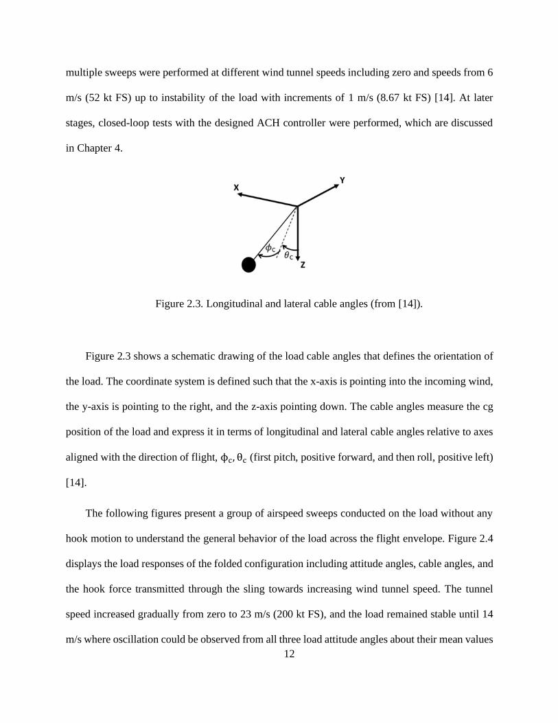
Figure 2.3 shows a schematic drawing of the load cable angles that defines the orientation of

the load. The coordinate system is defined such that the x-axis is pointing into the incoming wind,

the y-axis is pointing to the right, and the z-axis pointing down. The cable angles measure the cg

position of the load and express it in terms of longitudinal and lateral cable angles relative to axes

aligned with the direction of flight, ϕc, θc (first pitch, positive forward, and then roll, positive left)

[14].

The following figures present a group of airspeed sweeps conducted on the load without any

hook motion to understand the general behavior of the load across the flight envelope. Figure 2.4

displays the load responses of the folded configuration including attitude angles, cable angles, and

the hook force transmitted through the sling towards increasing wind tunnel speed. The tunnel

speed increased gradually from zero to 23 m/s (200 kt FS), and the load remained stable until 14

m/s where oscillation could be observed from all three load attitude angles about their mean values

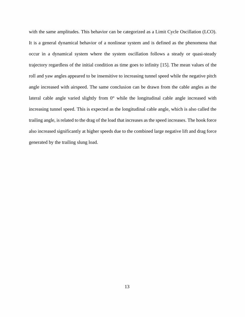
13

with the same amplitudes. This behavior can be categorized as a Limit Cycle Oscillation (LCO).

It is a general dynamical behavior of a nonlinear system and is defined as the phenomena that

occur in a dynamical system where the system oscillation follows a steady or quasi-steady

trajectory regardless of the initial condition as time goes to infinity [15]. The mean values of the

roll and yaw angles appeared to be insensitive to increasing tunnel speed while the negative pitch

angle increased with airspeed. The same conclusion can be drawn from the cable angles as the

lateral cable angle varied slightly from 0° while the longitudinal cable angle increased with

increasing tunnel speed. This is expected as the longitudinal cable angle, which is also called the

trailing angle, is related to the drag of the load that increases as the speed increases. The hook force

also increased significantly at higher speeds due to the combined large negative lift and drag force

generated by the trailing slung load.

14

Figure 2.4. Load attitude, cable angles, and hook force of the folded configuration during an

increase of the wind tunnel speed (from [14]).

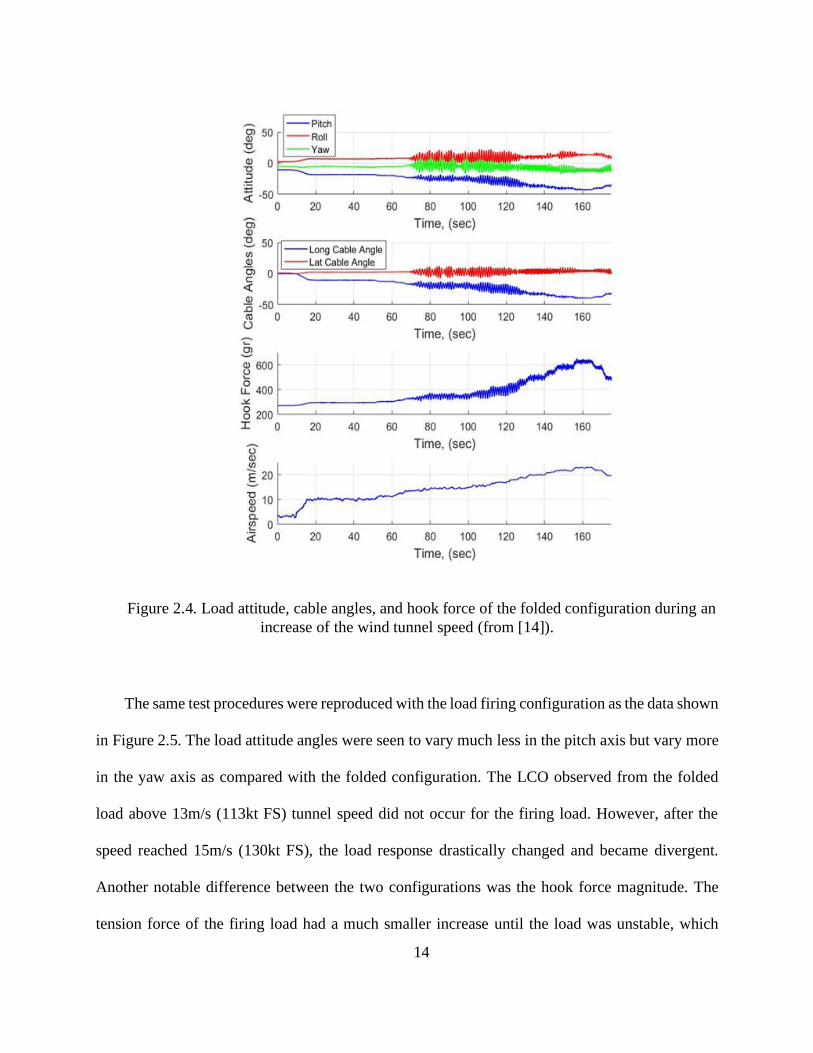
The same test procedures were reproduced with the load firing configuration as the data shown

in Figure 2.5. The load attitude angles were seen to vary much less in the pitch axis but vary more

in the yaw axis as compared with the folded configuration. The LCO observed from the folded

load above 13m/s (113kt FS) tunnel speed did not occur for the firing load. However, after the

speed reached 15m/s (130kt FS), the load response drastically changed and became divergent.

Another notable difference between the two configurations was the hook force magnitude. The

tension force of the firing load had a much smaller increase until the load was unstable, which

15

indicates the combined lift and drag forces from the load was much smaller as compared to the

folded load.

Figure 2.5. Load attitude, cable angles, and hook force of the firing configuration during an

increase of the wind tunnel speed (from [14]).

The airspeed sweep results shown for the two configurations demonstrate the stability issues

of the slung load during high-speed flights. An unstable load will induce oscillations in the

rotorcraft and penalize the handling and ride qualities. Also, large load oscillations can lead to the

load striking the rotorcraft fuselage, causing concern to flight safety.

16

2.2.2 Identification of Slung Load Linear Models

The open-loop tests showed the pendulum dynamics of the load oscillating about its steady-

state positions in stable or unstable fashions. In order to design a controller for active stabilization

of the load, dynamic models of the load response to ACH commands are required. As discussed

in [16], the frequency domain approach to system identification is a well-proven and well-suited

approach for identifying rotorcraft dynamics. By exciting the system with the correct type of input

with good spectral content, the frequency response can accurately characterize the system

dynamics and describe them with linear functions. For the commonly used inputs, frequency-

sweep inputs are the most reliable way to excite the system and provide frequency contents [16].

The term “frequency-sweep” refers to a class of control inputs that has a quasi-sinusoidal shape of

increasing frequency. The range of frequencies is strictly controlled by the operator to extract the

targeted dynamic mode and avoid excitation on other higher-order modes such as the dynamics of

the mechanical linkages. In this case, the hook was driven in either longitudinal or lateral direction

through the range of frequencies of interest to extract the load pendulum dynamics. Between the

speed from 0 to 14m/s (hover to 122 kt FS), frequency sweeps in longitudinal and lateral directions

found that linear models of the load pendulum motions could be identified based on the cable angle

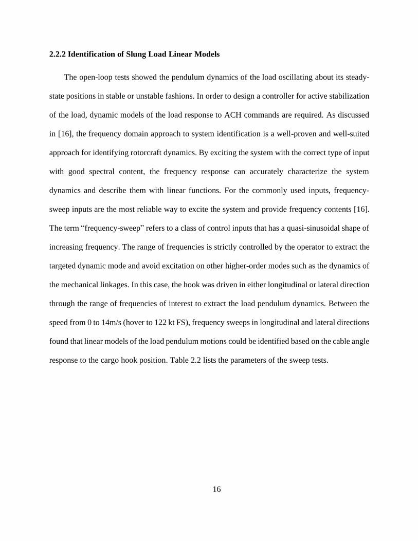
response to the cargo hook position. Table 2.2 lists the parameters of the sweep tests.

17

Parameters Model Scale Full Scale

Pendulum Length 273.6 mm 18.0 ft

Simple Pendulum

Frequency

6.00 rad/s 1.34 rad/s

Sweep Frequency

Range

0.22 to 53.7 rad/s 0.05 to 12 rad/s

Sweep Duration 44.7 sec 200 sec

Desired airspeed

Range

0 to 23 m/s 0 to 200 knots

Hook Position

Limits ±80 mm ±5.25 ft

Hook Rate Limits ±100 mm/s ±6.56 ft/s

Table 2.2. Frequency sweep test parameters (from [14]).

Researchers at TDD used CIFER and its associated utilities to process the data obtained

from the frequency-sweep tests and generated the corresponding frequency responses of the load

pendulum dynamics at each given speeds. The CIFER is an acronym for Comprehensive

Identification from Frequency Responses and it is a software developed by the TDD for system

identification based on the frequency response approach. The software includes core analysis

programs built around a sophisticated database, along with a set of user utilities for dynamics

studies of aeronautical systems [17]. The frequency responses were obtained using the advanced

Fast Fourier Transform (FFT) algorithm and the associated windowing techniques implemented

in CIFER® [16].

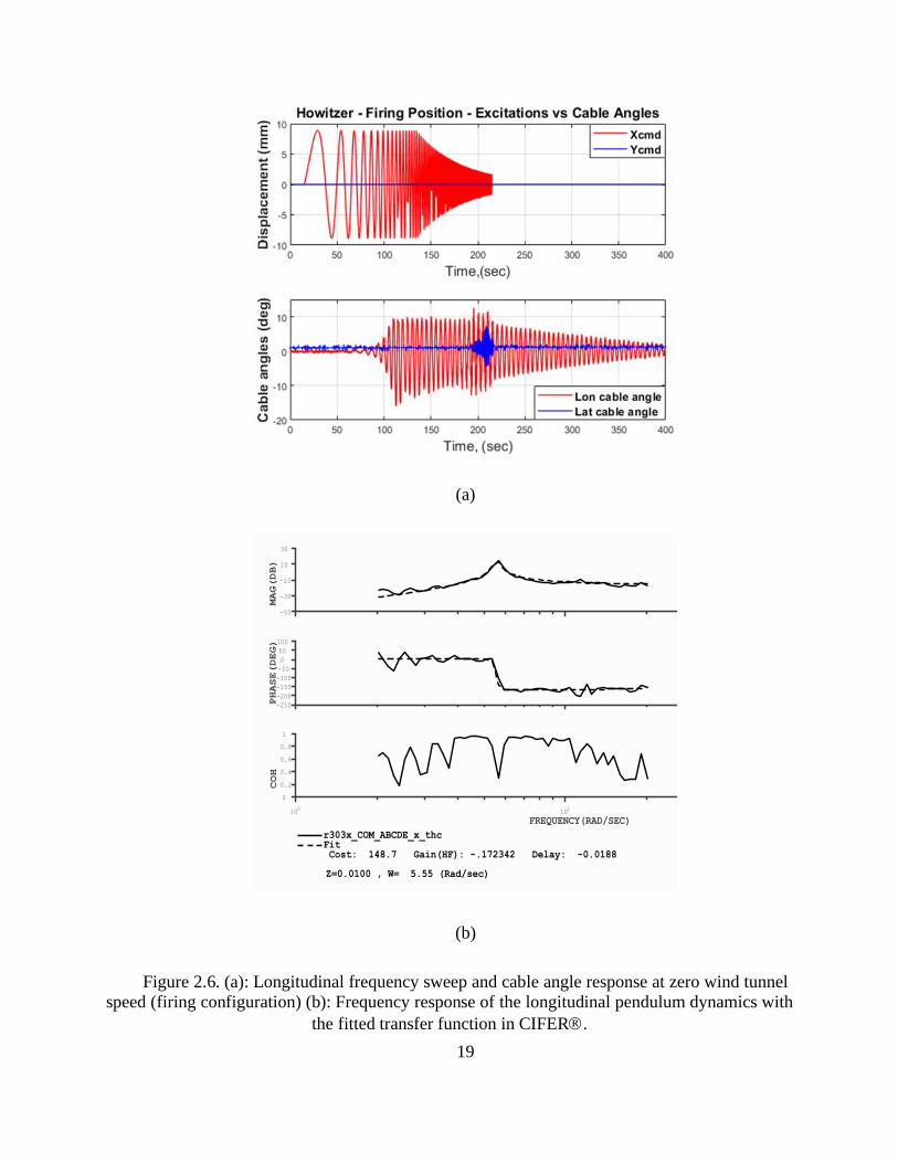
A selected case of the frequency-sweep tests at zero tunnel speed is presented in the following.

Figure 2.6(a) shows the hook being driven longitudinally and the corresponding cable angle

response. The hook input amplitude started at 9 mm (0.6 ft FS) and gradually decreased after 11.4

rad/s to avoid exceeding the hook rate limit. The actuator of the moving hook was found to have

18

good linear input/output response and excellent signal to noise ratio out to 20 rad/s as identified

from its frequency response [14]. The cable angle response showed mainly on-axis (𝜃𝑐/𝑥, 𝜙𝑐/𝑦)

response to the motion of the hook and the off-axis (𝜃𝑐/𝑦, 𝜙𝑐/𝑥) correlation was found to be small

for both longitudinal and lateral pendulum dynamics.

The frequency response of the longitudinal cable angle is shown in Figure 2.6(b) along with

the fitted transfer function represented by the black dash line. The transfer-function modeling is a

function provided by CIFER® that compose parametric models of the system dynamics and

express them in the form of transfer functions. The values of the transfer-function gain, pole

locations, and zero locations are determined numerically to provide the best match (in a least-

squares sense) to the frequency-response data [16]. The correlation between the two curves shows

good accuracy over the range of 2 to 20 rad/s with an identification cost of 148.7. The coherence

provides a key measure of the quality of data from the frequency-response. It indicates whether

the system has been satisfactorily excited across the entire frequency range and shows whether the

system being modeled is well characterized as a linear process in this frequency range [16]. Usually,

a coherence above 0.6 represents good accuracy at the corresponding frequency. The cost function

indicates the level of accuracy of the fitted transfer function. A cost function smaller than 100

generally reflects an acceptable level of accuracy for dynamics modeling [16]. The parameters of

the transfer function are listed at the bottom of figure (b). Symbols Z and W represent the damping

and the natural frequency of a 2nd order linear system along with a delay factor in seconds that

account for unknown delays and higher dynamics in the system.

19

(a)

(b)

Figure 2.6. (a): Longitudinal frequency sweep and cable angle response at zero wind tunnel

speed (firing configuration) (b): Frequency response of the longitudinal pendulum dynamics with

the fitted transfer function in CIFER.

r303x_COM_ABCDE_x_thcFit Cost: 148.7 Gain(HF): -.172342 Delay: -0.0188

Z=0.0100 , W= 5.55 (Rad/sec)

-50

-30

-10

10

30

MAG(DB)

-250

-200

-150

-100

-50

0

50

100

PHASE(DEG)

100

101

FREQUENCY(RAD/SEC)

0

0.2

0.4

0.6

0.8

1

COH

20

(a)

(b)

Figure 2.7. (a): Lateral frequency sweep and cable angle response at zero wind tunnel speed

(firing configuration). (b): Frequency response of the lateral pendulum dynamics with the fitted

transfer function in CIFER.

21

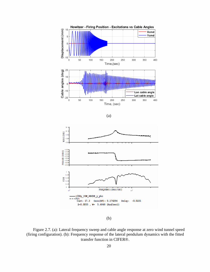
Figure 2.7 shows the same frequency sweep in the lateral direction. The lateral load pendulum

motion showed less off-axis dynamics compared to the longitudinal pendulum motion as the

longitudinal cable angle reacted slightly to the hook excitation. The frequency response also

showed better agreement with the fitted transfer function with a much lower cost of 17.3, which

indicates that the transfer function produced a match that is nearly indistinguishable from the

frequency-response data. For both longitudinal and lateral load pendulum dynamics, the damping

ratios were found to be small and the identified pendulum frequencies were close to the expected

pendulum frequency of 6 rad/s.

𝜃𝑐

𝑥,𝜙𝑐

𝑦 =

𝐾𝑝𝑠2

(𝑠2 + 2𝜁𝑝𝜔𝑝 𝑠 + 𝜔𝑝2)

𝑒−𝑠∗𝜏 (2.2)

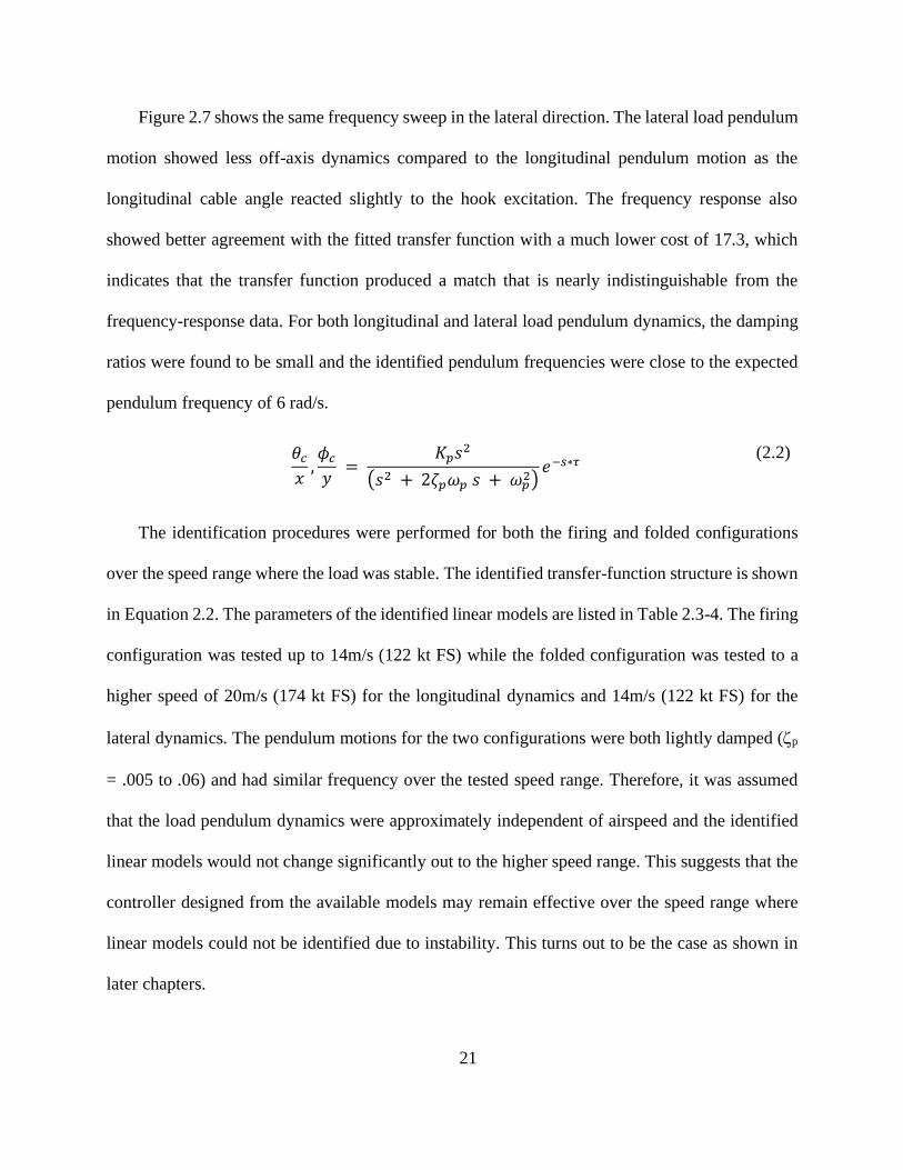
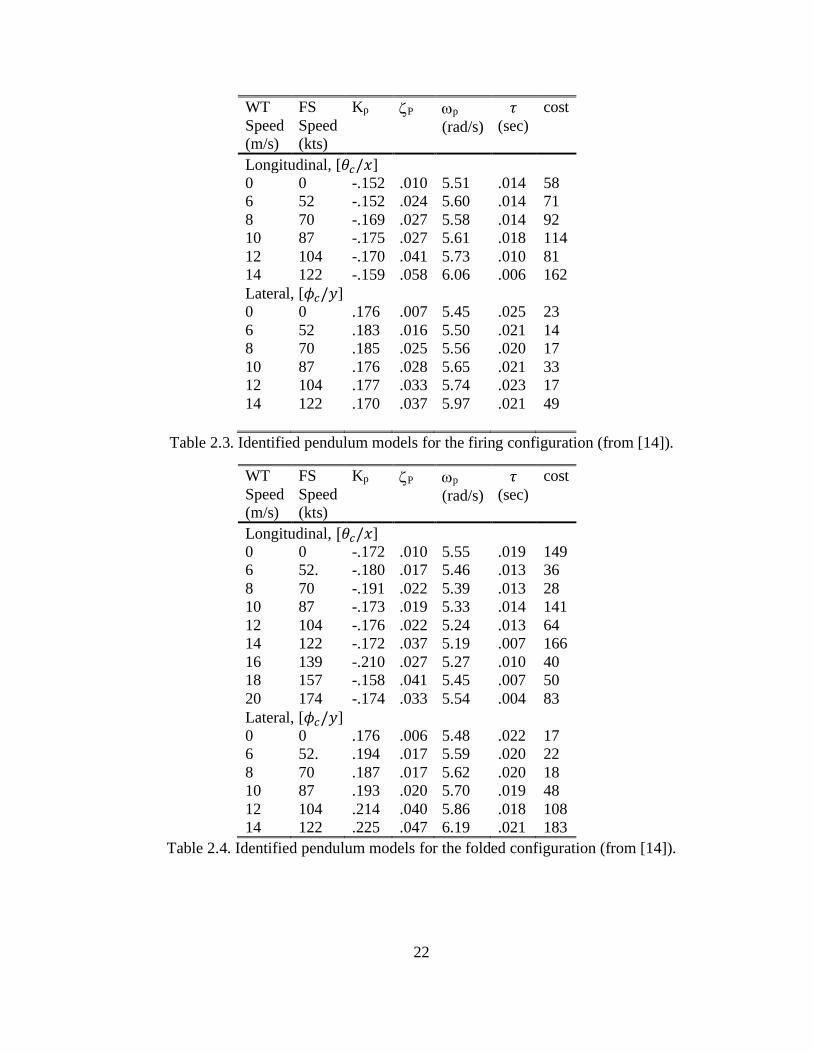
The identification procedures were performed for both the firing and folded configurations

over the speed range where the load was stable. The identified transfer-function structure is shown

in Equation 2.2. The parameters of the identified linear models are listed in Table 2.3-4. The firing

configuration was tested up to 14m/s (122 kt FS) while the folded configuration was tested to a

higher speed of 20m/s (174 kt FS) for the longitudinal dynamics and 14m/s (122 kt FS) for the

lateral dynamics. The pendulum motions for the two configurations were both lightly damped (p

= .005 to .06) and had similar frequency over the tested speed range. Therefore, it was assumed

that the load pendulum dynamics were approximately independent of airspeed and the identified

linear models would not change significantly out to the higher speed range. This suggests that the

controller designed from the available models may remain effective over the speed range where

linear models could not be identified due to instability. This turns out to be the case as shown in

later chapters.

22

WT

Speed

(m/s)

FS

Speed

(kts)

Kp

P p

(rad/s)

𝜏

(sec)

cost

Longitudinal, [𝜃𝑐/𝑥]

0 0 -.152 .010 5.51 .014 58

6 52 -.152 .024 5.60 .014 71

8 70 -.169 .027 5.58 .014 92

10 87 -.175 .027 5.61 .018 114

12 104 -.170 .041 5.73 .010 81

14 122 -.159 .058 6.06 .006 162

Lateral, [𝜙𝑐/𝑦]

0 0 .176 .007 5.45 .025 23

6 52 .183 .016 5.50 .021 14

8 70 .185 .025 5.56 .020 17

10 87 .176 .028 5.65 .021 33

12 104 .177 .033 5.74 .023 17

14 122 .170 .037 5.97 .021 49

Table 2.3. Identified pendulum models for the firing configuration (from [14]).

WT

Speed

(m/s)

FS

Speed

(kts)

Kp

P p

(rad/s)

𝜏

(sec)

cost

Longitudinal, [𝜃𝑐/𝑥]

0 0 -.172 .010 5.55 .019 149

6 52. -.180 .017 5.46 .013 36

8 70 -.191 .022 5.39 .013 28

10 87 -.173 .019 5.33 .014 141

12 104 -.176 .022 5.24 .013 64

14 122 -.172 .037 5.19 .007 166

16 139 -.210 .027 5.27 .010 40

18 157 -.158 .041 5.45 .007 50

20 174 -.174 .033 5.54 .004 83

Lateral, [𝜙𝑐/𝑦]

0 0 .176 .006 5.48 .022 17

6 52. .194 .017 5.59 .020 22

8 70 .187 .017 5.62 .020 18

10 87 .193 .020 5.70 .019 48

12 104 .214 .040 5.86 .018 108

14 122 .225 .047 6.19 .021 183

Table 2.4. Identified pendulum models for the folded configuration (from [14]).

23

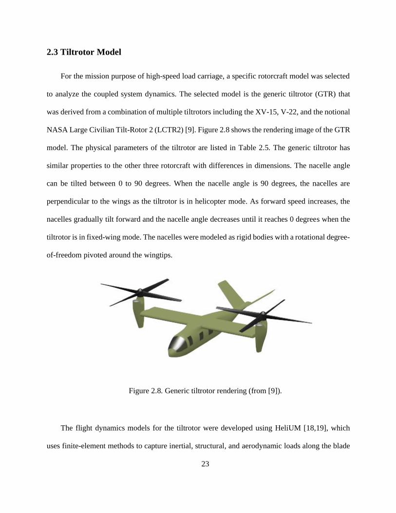
2.3 Tiltrotor Model

For the mission purpose of high-speed load carriage, a specific rotorcraft model was selected

to analyze the coupled system dynamics. The selected model is the generic tiltrotor (GTR) that

was derived from a combination of multiple tiltrotors including the XV-15, V-22, and the notional

NASA Large Civilian Tilt-Rotor 2 (LCTR2) [9]. Figure 2.8 shows the rendering image of the GTR

model. The physical parameters of the tiltrotor are listed in Table 2.5. The generic tiltrotor has

similar properties to the other three rotorcraft with differences in dimensions. The nacelle angle

can be tilted between 0 to 90 degrees. When the nacelle angle is 90 degrees, the nacelles are

perpendicular to the wings as the tiltrotor is in helicopter mode. As forward speed increases, the

nacelles gradually tilt forward and the nacelle angle decreases until it reaches 0 degrees when the

tiltrotor is in fixed-wing mode. The nacelles were modeled as rigid bodies with a rotational degree-

of-freedom pivoted around the wingtips.

Figure 2.8. Generic tiltrotor rendering (from [9]).

The flight dynamics models for the tiltrotor were developed using HeliUM [18,19], which

uses finite-element methods to capture inertial, structural, and aerodynamic loads along the blade

24

segment. The aerodynamics of each component including the blade, wing, and fuselage came from

nonlinear lookup tables, and the rotor air-wakes were modeled using a dynamic inflow model. The

modeling accuracy from HeliUM was validated for various aircraft, the results of all these

validation efforts provide confidence in the modeling fidelity for the generic tiltrotor model [9].

Aircraft Data

Gross Weight 32,100 lbs

Max Continuous Power (SL) 9,400 hp

Maximum Speed (VTAS) 280 kts

Wing Span 45 ft

Wing Sweep 0 deg

Nacelle Range 0 – 90 deg

Rotor Data

Radius 17.8 feet

Number of Blades/Rotor 4

Rotational Speed 40-30 rad/sec

Precone 2.5 deg

Twist -44 deg

Table 2.5. Tiltrotor Configuration Data (from [9]).

To provide a MATLAB simulation model that is capable of faster-than-real-time execution

speeds, linear models, and trim data were extracted from HeliUM and used to develop a stitched

model of the generic tiltrotor. The tiltrotor linear models contain 51 states and 9 control inputs that

are listed as the following.

51 tiltrotor states:

• Fuselage states (𝑢, 𝑣, 𝑤, 𝑝, 𝑞, 𝑟, 𝜙𝑇 , 𝜃𝑇 , 𝜓𝑇)

• Rotor states per rotor (𝜁0, 𝜁1𝑐 , 𝜁1𝑠, 𝜁2, 𝜁0, 𝜁1𝑐 , 𝜁1𝑠 , 𝜁2, ��0, ��1𝑐 , ��1𝑠, ��2, 𝛽0, 𝛽1𝑐 , 𝛽1𝑠, 𝛽2)

• Inflow states per rotor (𝜆0, 𝜆1𝑐 , 𝜆1𝑠)

• Nacelle states per nacelle (nacelle angle and nacelle angular rate)

25

9 control inputs:

• Symmetric phased lateral cyclic (𝜃1𝑐′ )

• Differential collective (∆𝜃0)

• Symmetric phased longitudinal cyclic (𝜃1𝑠′ )

• Symmetric collective (𝜃0)

• Differential phased longitudinal cyclic (Δ𝜃1𝑠′ )

• Aileron (𝛿𝑎)

• Elevator (𝛿𝑒)

• Rudder (𝛿𝑟)

• Symmetric nacelle angle (𝛿𝑛𝑎𝑐)

The rotor states reflect four second-order rotor dynamics for each of the two-blade modes

associated with each rotor. The nacelle states contain two second-order nacelle rotational dynamics

for each nacelle. The stitched model is stitched in total x body axis velocity 𝑢 and symmetric

nacelle angle 𝛿𝑛𝑎𝑐 [9], and it can be trimmed, simulated, and linearized at any flight condition

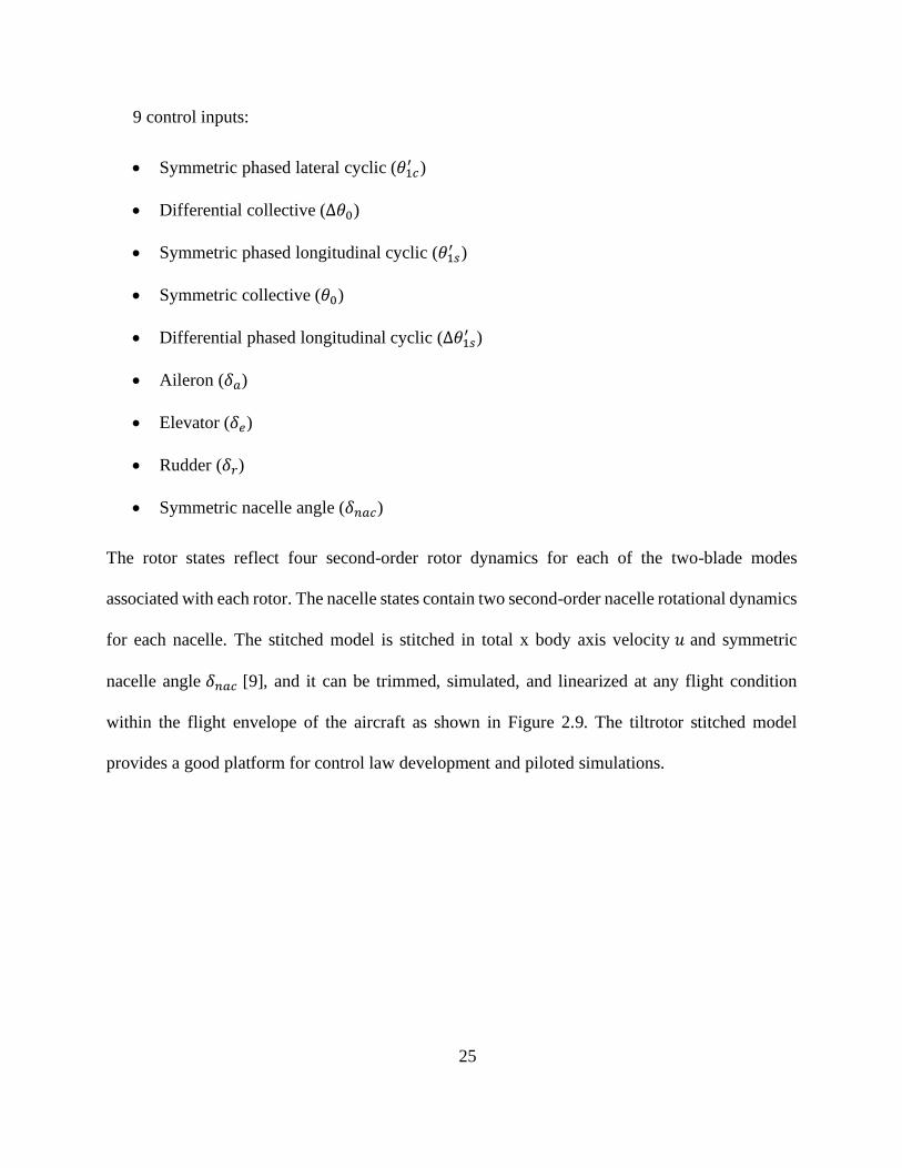
within the flight envelope of the aircraft as shown in Figure 2.9. The tiltrotor stitched model

provides a good platform for control law development and piloted simulations.

26

Figure 2.9. GTR Stitched model conversion corridor and linear model points.

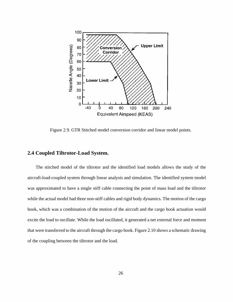
2.4 Coupled Tiltrotor-Load System.

The stitched model of the tiltrotor and the identified load models allows the study of the

aircraft-load-coupled system through linear analysis and simulation. The identified system model

was approximated to have a single stiff cable connecting the point of mass load and the tiltrotor

while the actual model had three non-stiff cables and rigid body dynamics. The motion of the cargo

hook, which was a combination of the motion of the aircraft and the cargo hook actuation would

excite the load to oscillate. While the load oscillated, it generated a net external force and moment

that were transferred to the aircraft through the cargo hook. Figure 2.10 shows a schematic drawing

of the coupling between the tiltrotor and the load.

27

Figure 2.10. Schematic diagram of the tiltrotor-load coupled system.

The control allocation module transforms the pilot inputs into mechanical inputs on the

rotorcraft. The pilot inputs consist of lateral cyclic (𝑢𝑙𝑎𝑡), longitudinal cyclic (𝑢𝑙𝑜𝑛), collective

(𝑢𝑐𝑜𝑙) and pedal (𝑢𝑝𝑒𝑑). The transformation follows the same procedure in Ref. [20], in which it

uses a control allocation structure similar to the XV-15 tiltrotor.

The tiltrotor stitched model contains the trim data and linearized model at the desired flight

condition. The block receives pilot input and outputs system states 𝑋𝑇𝑅 . The next block uses the

state variables to compute the acceleration of the cargo hook in the longitudinal and lateral

directions. The cargo hook accelerations are then transmitted to the linear model of the slung load,

which outputs the load cable angles. Lastly, the Cable Force and Moment block calculate the

external force and moment based on the cable angles and aircraft states, and by feeding back the

force and moment terms, the load is coupled to the aircraft. Previous sections have discussed the

Tiltrotor Stitched Model and the Slung Load Dynamics blocks in the figure, and the following

section will disclose the calculation of the Cargo Hook Velocity and Acceleration and the Cable

Force and Moment blocks.

28

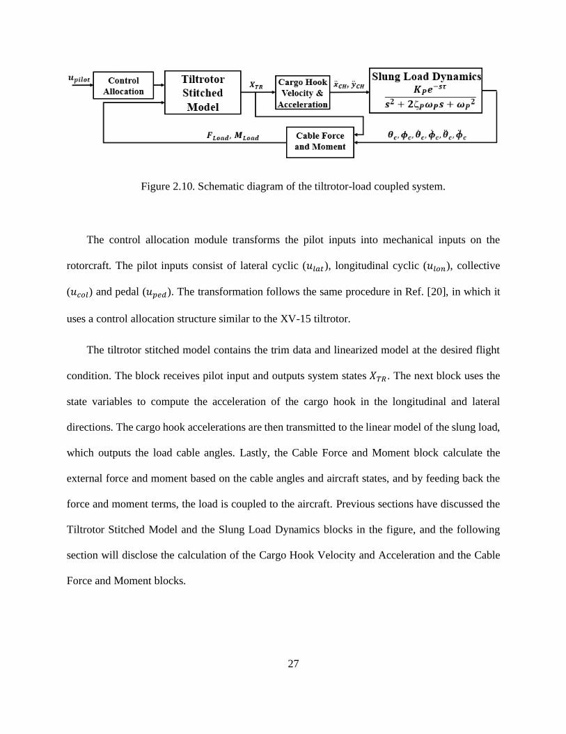
Figure 2.11. Coordinate systems of the tiltrotor-load coupled model.

The computation of the hook velocity and acceleration requires expressing the terms in the

inertial coordinate system. Therefore, the hook velocity and acceleration were first calculated and

expressed in the aircraft body frame and later transformed into the inertial frame. Figure 2.11

shows the inertial coordinate system (𝑥𝐸, 𝑦𝐸 , 𝑧𝐸) and the body coordinate system (𝑥𝑏, 𝑦𝑏 , 𝑧𝑏). The

nominal attachment point of the cargo hook (with no actuation) is indicated by CH and the actual

position of the hook (with actuation) is represented by A. The distance between points CH and A

is expressed by 𝑟∆ that represents the hook actuation away from the attachment point. The vector

𝑟𝐶𝐻 measures the location of the cargo hook attachment point from the center of gravity of the

aircraft. The vector 𝑟𝐴 expresses the location of the cargo hook in the inertial frame, which is the

29

frame of interest to measure the location of the cargo hook. The derivation of the vector 𝑟𝐴 is shown

in the following equations that include transformation and conversion between the two reference

frames and the associated coordinate systems.

𝑟𝐴 =𝑟𝐶𝐺 +𝑟𝐶𝐻 + 𝑟∆ (2.3)

Taking the derivatives of both sides of the equation:

𝑣𝐴𝑒

= 𝑣𝐶𝐺𝑏

+ ��𝐶𝐻

𝑏+ ��𝑏/𝑒 × 𝑟𝐶𝐻

𝑏+ ��∆

𝑏+ ��𝑏/𝑒 × 𝑟∆

𝑏 (2.4)

Vector 𝑟𝐶𝐻 is fixed in the body frame, therefore, ��𝐶𝐻

𝑏= 0. The acceleration of the cargo hook

position A can be derived as the following:

��𝐴𝑒

= ��𝐶𝐺

𝑏+ ��𝑏/𝑒 × 𝑣𝐶𝐺

𝑏+ (��𝑏/𝑒 + ��𝑏/𝑒 × ��𝑏/𝑒) × 𝑟𝐶𝐻

𝑏

+ ��𝑏/𝑒 × (��𝐶𝐻

𝑏+ ��𝑏/𝑒 × 𝑟𝐶𝐻

𝑏) + ��∆

𝑏+ ��𝑏/𝑒 × ��∆

𝑏

+ (��𝑏/𝑒 × ��𝑏/𝑒) × 𝑟∆𝑏

+ ��𝑏/𝑒 × 𝑟∆𝑏

+ ��𝑏/𝑒 × (��∆

𝑏

+ ��𝑏/𝑒 × 𝑟∆𝑏

)

(2.5)

The cross product between a vector with itself is equal to 0. Hence, simplifying the expression and

eliminating the zero terms, the expression of the cargo hook acceleration in the inertial coordinate

is:

��𝐴𝑒

= ��𝐶𝐺

𝑏+ ��𝑏/𝑒 × 𝑣𝐶𝐺

𝑏+ ��𝑏/𝑒 × (𝑟𝐶𝐻

𝑏+ 𝑟∆

𝑏)

+ ��𝑏/𝑒 × [��𝑏/𝑒 × (𝑟𝐶𝐻𝑏

+ 𝑟∆𝑏

)] + ��Δ

𝑏+ 2��𝑏/𝑒 × ��∆

𝑏

(2.6)

While the velocity, acceleration, and rotational speed of the rotorcraft are expressed as the

following:

30

𝑣𝐶𝐺𝑏

= [𝑢, 𝑣, 𝑤], ��𝐶𝐺

𝑏= [��, ��, ��], ��𝑏/𝑒 = [𝑝, 𝑞, 𝑟] (2.7)

The cargo hook actuation, velocity, and acceleration are:

𝑟∆𝑏

= [𝑥𝐶𝐻𝑏, 𝑦𝐶𝐻 𝑏

], ��∆

𝑏= [��𝐶𝐻𝑏

, ��𝐶𝐻 𝑏], ��∆

𝑏= [��𝐶𝐻𝑏

, ��𝐶𝐻𝑏] (2.8)

Notice the [��𝐶𝐻𝑏, ��𝐶𝐻 𝑏

] in Equation 2.8 are different than the terms in Figure 2.10. The former

represents the accelerations of the cargo hook actuation measured in the body frame and the latter

is the accelerations measured in the inertial frame and expressed in body coordinates.

The hook accelerations are then taken as input by the linear load model to compute the load

cable angles. The transfer function block essentially appends 4 extra states, which are derived from

the two second-order load pendulum models, to the GTR stitched model. The cable-angle states

combined with tiltrotor states will compute the external force transferred to the cargo hook that is

generated by the load. The trim cable force measured from the wind tunnel test will account for

both the aerodynamic and inertial forces of the load. It was assumed that dynamic force increments

were only due to the load inertial force computed from the linear acceleration and that the load

aerodynamic force was assumed to be unchanged from the trim value. While coupled with the

rotorcraft, the cable angles need to be expressed relative to the tiltrotor such that the action of the

rotorcraft is taken into account. The identified load transfer function outputs the cable angles as if

they are measured in the inertial frame. However, the desired cable angles should be expressed

relative to the rotorcraft body-fixed frame since the force and moment are computed by the relative

motion between the load and the tiltrotor. The derivations of the relative acceleration and the cable

angles between the load and the rotorcraft are described below.

31

In Figure 2.11, the position vector of the load center of mass can be written as the following

where 𝑙 indicates the length of the hypothetical line between the cargo hook and the load center of

gravity:

𝑙𝑒 = 𝑙 ∙ [𝐶𝜙𝑐𝑆𝜃𝑐

−𝑆𝜙𝑐

𝐶𝜙𝑐𝐶𝜃𝑐

]

(2.9)

C and S represent operations of cos and sin. The velocity vector of the cable can be expressed as:

𝑙𝐸

𝑒

= 𝑙 ∙ [

−��𝑐𝑆𝜙𝑐𝑆𝜃𝑐 + ��𝑐𝐶𝜙𝑐𝐶𝜃𝑐

−��𝑐𝐶𝜙𝑐

−��𝑐𝑆𝜙𝑐𝐶𝜃𝑐 − ��𝑐𝐶𝜙𝑐𝑆𝜃𝑐

]

(2.10)

The subscript E indicates that the derivative is taken in the inertial (Earth) frame. The acceleration

vector of the cable can be expressed as:

𝑙𝐸

𝑒

= 𝑙 ∙ [

−𝜙��𝑆𝜙𝑐𝑆𝜃𝑐 − ��𝑐2

𝐶𝜙𝑐𝑆𝜃𝑐 − ��𝑐��𝑐𝑆𝜙𝑐𝐶𝜃𝑐 + 𝜃��𝐶𝜙𝑐𝐶𝜃𝑐 − ��𝑐��𝑐𝑆𝜙𝑐𝐶𝜃𝑐 − ��𝑐2

𝐶𝜙𝑐𝑆𝜃𝑐

−𝜙��𝑆𝜙𝑐 + ��𝑐2𝐶𝜙𝑐

−𝜙��𝑆𝜙𝑐𝐶𝜃𝑐 − ��𝑐2𝐶𝜙𝑐𝐶𝜃𝑐 + ��𝑐��𝑐𝑆𝜙𝑐𝑆𝜃𝑐 − 𝜃��𝐶𝜙𝑐𝑆𝜃𝑐 + ��𝑐��𝑐𝑆𝜙𝑐𝑆𝜃𝑐 − ��𝑐

2𝐶𝜙𝑐𝐶𝜃𝑐

]

(2.11)

Based on Poisson’s kinematical equations [21], the position, velocity, and acceleration vectors of

the cable could be expressed in the rotorcraft body frame as:

𝑙𝑏 = ��𝐸𝐵𝑙𝑒 (2.12)

𝑙𝐸

𝑏

= ��𝐸𝐵𝑙𝑒 + ��𝐸𝐵𝑙𝑒

𝑒

= −��𝑏/𝑒��𝐸𝐵𝑙𝑒 + ��𝐸𝐵𝑙𝐸

𝑒

(2.13)

𝑙𝐸

𝑏

= ��𝐸𝐵𝑙𝐸

𝑒

+ 2��𝐸𝐵𝑙𝐸

𝑒

+ ��𝐸𝐵𝑙𝐸

𝑒

= (��𝑏/𝑒2 − ��𝑏/𝑒 − 2��𝑏/𝑒)��𝐸𝐵𝑙

𝐸

𝑒

+ ��𝐸𝐵𝑙𝐸

𝑒

(2.14)

32

Where ��𝐸𝐵 is the Inertial to body coordinate transform matrix and is calculated following the order

yaw (𝜓), pitch (𝜃), and roll (𝜙):

��𝐸𝐵 = [𝐶𝜃𝑇𝐶𝜓𝑇 𝐶𝜃𝑇𝑆𝜓𝑇 −𝑆𝜃𝑇

−𝐶𝜙𝑇𝑆𝜓𝑇 + 𝑆𝜙𝑇𝑆𝜃𝑇𝐶𝜓𝑇 𝐶𝜙𝑇𝐶𝜓𝑇 + 𝑆𝜙𝑇𝑆𝜃𝑇𝑆𝜓𝑇 𝑆𝜙𝑇𝐶𝜃𝑇

𝑆𝜙𝑇𝑆𝜓𝑇 + 𝐶𝜙𝑇𝑆𝜃𝑇𝐶𝜓𝑇 −𝑆𝜙𝑇𝐶𝜓𝑇 + 𝐶𝜙𝑇𝑆𝜃𝑇𝑆𝜓𝑇 𝐶𝜙𝑇𝐶𝜃𝑇

]

(2.15)

The rotation angles are described by the tiltrotor attitude angles (𝜓𝑇, 𝜃𝑇, 𝜙𝑇). ��𝑏/𝑒 and ��𝑏/𝑒 are

the angular velocity and acceleration of the tiltrotor relative to the inertial frame expressed in

matrix form:

��𝑏/𝑒 = [0 −𝑟 𝑞𝑟 0 −𝑝

−𝑞 𝑝 0]

(2.16)

��𝑏/𝑒 = [0 −�� 0 −��

−�� 0]

(2.17)

Combing the equations listed above, the relative velocity and acceleration between the load and

the aircraft can be written as the following:

𝑣𝐿

𝑒= 𝑙

𝐸

𝑏

+ ��𝑏/𝑒𝑙𝑏 (2.18)

��𝐿

𝑒= 𝑙

𝐸

𝑏

+ 2��𝑏/𝑒𝑙𝐸

𝑏

+ ��𝑏/𝑒𝑙𝑏 + ��𝑏/𝑒 × (��𝑏/𝑒 × 𝑙𝑏) (2.19)

The relative cable angles are expressed as:

𝜃𝑐 = atan (

𝑙𝑥

𝑙𝑧)

(2.20)

𝜙𝑐 = −asin (

𝑙𝑦

𝑙)

(2.21)

The external force applied to the cargo hook that was generated by the load is described below:

33

��𝐿 = �� + ��𝑎𝑒𝑟𝑜 + ��𝑖𝑛𝑒𝑟𝑡𝑖𝑎𝑙 = �� − 𝑚𝐿��𝐿𝑒

(2.22)

Where vector �� contains the recorded hook force from the wind tunnel test that accounts for the

weight and the aerodynamic force. The term 𝑚𝐿��𝐿𝑒 represents the load inertial force and it has the

opposite direction to the trim cable tension force. The external moment can be calculated based on

the external force and the hook position.

2.5 Linear Analysis of System Stability

The linearized GTR stitched model has 51 states which include rotor dynamics, inflow,

fuselage rigid body dynamics, and the nacelle angle dynamics. For the bare aircraft model, the yaw

angle 𝜓 was completely decoupled from the rest of the states, hence, the yaw attitude was simply

removed from the full order system for linear analysis. The rest of the states were divided into two

categories that represent the fast and slow dynamics of the system. The fast dynamics including

rotor, inflow, and the nacelle angle dynamics, were assumed to reach steady-state much faster than

the fuselage states. The slow dynamics represent the rigid body modes of the rotorcraft that are of

major interest as they have lower frequencies in the range important for handling qualities and are

unstable at low airspeed flight.

For the bare-airframe model, the full-order model is reduced to an 8-state model to decouple

the effects from the rotor states on the fuselage states. The model order reduction process can be

formulated as the following.

𝑋 = [𝑋𝑠𝑙𝑜𝑤 , 𝑋𝑓𝑎𝑠𝑡] (2.23)

𝑋𝑠𝑙𝑜𝑤 = [𝑢, 𝑣, 𝑤, 𝑝, 𝑞, 𝑟, ϕ, 𝜃] (2.24)

34

𝑋𝑓𝑎𝑠𝑡 = [𝑟𝑜𝑡𝑜𝑟 𝑠𝑡𝑎𝑡𝑒𝑠, 𝑖𝑛𝑓𝑙𝑜𝑤 𝑠𝑡𝑎𝑡𝑒𝑠, 𝑛𝑎𝑐𝑒𝑙𝑙𝑒 𝑎𝑛𝑔𝑙𝑒 𝑠𝑡𝑎𝑡𝑒𝑠] (2.25)

�� = [

𝐴11 𝐴12

𝐴21 𝐴22] ∗ [𝑋𝑠𝑙𝑜𝑤 , 𝑋𝑓𝑎𝑠𝑡]𝑇 + [

𝐵1

𝐵2] ∗ 𝑢

(2.26)

��𝑠𝑙𝑜𝑤 = �� ∗ 𝑋𝑠𝑙𝑜𝑤 + �� ∗ 𝑋𝑠𝑙𝑜𝑤 (2.27)

�� = 𝐴11 − 𝐴12𝐴22−1𝐴21, �� = 𝐵1 − 𝐴12𝐴22

−1𝐵2 (2.28)

The reduced model contains only the rigid body modes of the aircraft and they have much

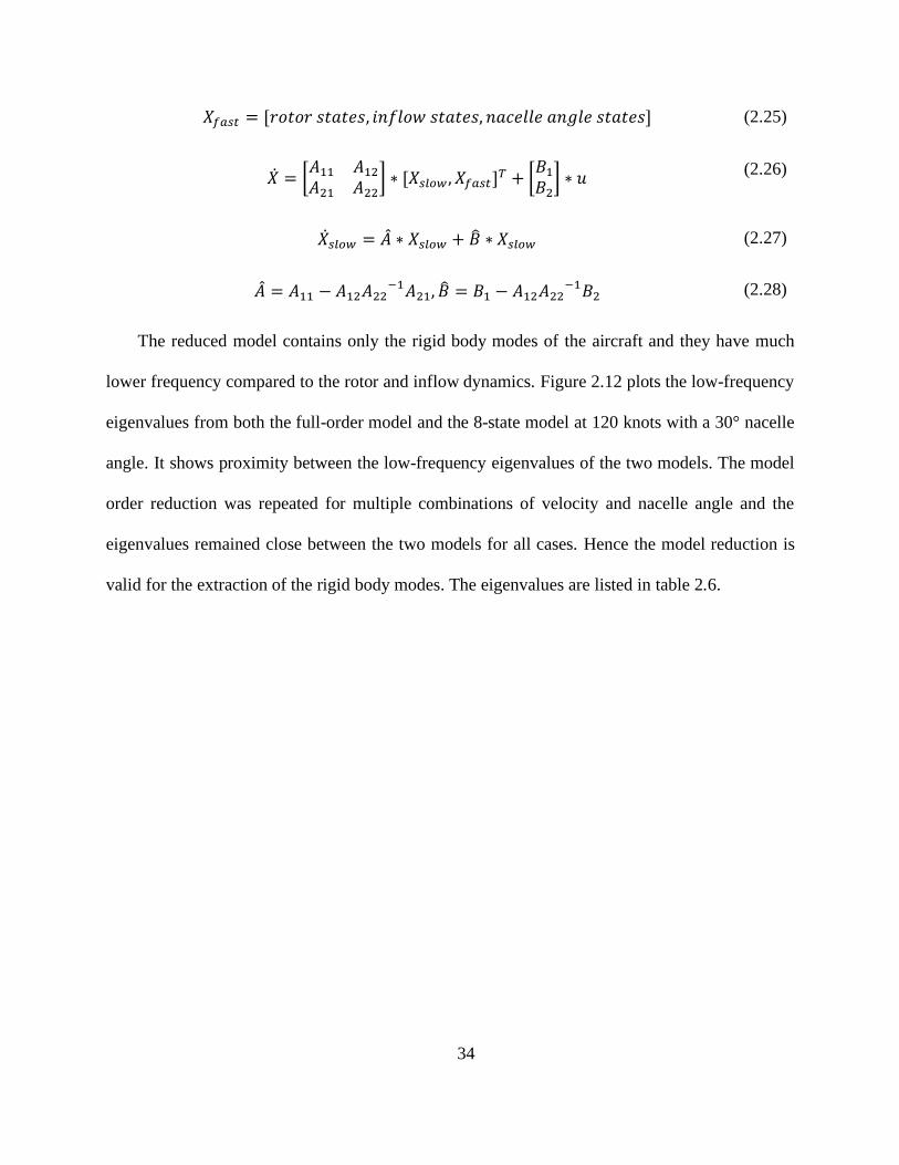
lower frequency compared to the rotor and inflow dynamics. Figure 2.12 plots the low-frequency

eigenvalues from both the full-order model and the 8-state model at 120 knots with a 30° nacelle

angle. It shows proximity between the low-frequency eigenvalues of the two models. The model

order reduction was repeated for multiple combinations of velocity and nacelle angle and the

eigenvalues remained close between the two models for all cases. Hence the model reduction is

valid for the extraction of the rigid body modes. The eigenvalues are listed in table 2.6.

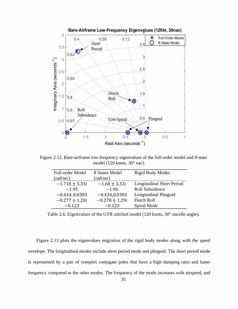
35

Figure 2.12. Bare-airframe low-frequency eigenvalues of the full-order model and 8-state

model (120 knots, 30° nac).

Full-order Model

(rad/sec)

8 States Model

(rad/sec)

Rigid Body Modes

−1.718 ± 3.33𝑖 −1.68 ± 3.32𝑖 Longitudinal Short Period

−1.95 −1.96 Roll Subsidence

−0.434, 0.0383 −0.434,0.0383 Longitudinal Phugoid

−0.277 ± 1.28𝑖 −0.278 ± 1.29𝑖 Dutch Roll

−0.123 −0.123 Spiral Mode

Table 2.6. Eigenvalues of the GTR stitched model (120 knots, 30° nacelle angle).

Figure 2.13 plots the eigenvalues migration of the rigid body modes along with the speed

envelope. The longitudinal modes include short period mode and phugoid. The short period mode

is represented by a pair of complex conjugate poles that have a high damping ratio and faster

frequency compared to the other modes. The frequency of the mode increases with airspeed, and

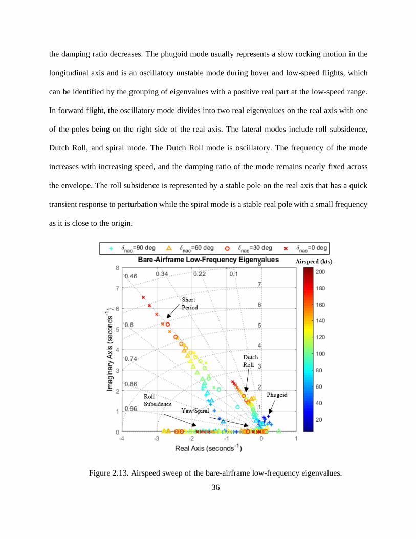
36

the damping ratio decreases. The phugoid mode usually represents a slow rocking motion in the

longitudinal axis and is an oscillatory unstable mode during hover and low-speed flights, which

can be identified by the grouping of eigenvalues with a positive real part at the low-speed range.

In forward flight, the oscillatory mode divides into two real eigenvalues on the real axis with one

of the poles being on the right side of the real axis. The lateral modes include roll subsidence,

Dutch Roll, and spiral mode. The Dutch Roll mode is oscillatory. The frequency of the mode

increases with increasing speed, and the damping ratio of the mode remains nearly fixed across

the envelope. The roll subsidence is represented by a stable pole on the real axis that has a quick

transient response to perturbation while the spiral mode is a stable real pole with a small frequency

as it is close to the origin.

Figure 2.13. Airspeed sweep of the bare-airframe low-frequency eigenvalues.

37

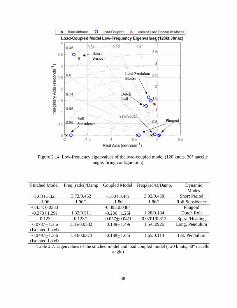
The coupled system contains two extra second-order equations from the load longitudinal and

lateral transfer functions, which results in four extra states to be included by the system as shown

in Equation 2.29. Figure 2.14 shows the eigenvalues of the load-coupled system being plotted

alongside the bare-airframe model. From the plot, it can be seen that the coupling effect between

the load and the rotorcraft at such airspeed is fairly small, as indicated by the proximity between

the poles of the isolated and coupled systems. As listed in table 2.7, the comparison between the

eigenvalues of the same mode before and after coupling the load can draw some insight into how

the system dynamics are changed due to the coupling effect. The longitudinal short period mode

shows a small increase of its damping ratio (from 0.452 to 0.458) and frequency (from 3.72 rad/s

to 3.92 rad/s). The lateral Dutch Roll mode has its damping ratio decreased from 0.211 to 0.184

and frequency from 1.32 rad/s to 1.28 rad/s. The Yaw/Spiral mode becomes an oscillatory mode

after the load is added as the aircraft heading angle is now coupled into the system dynamics. In a

general view, the aircraft is destabilized due to the coupling effect as the damping ratios of the

low-frequency modes are decreased. The damping ratio of the longitudinal pendulum mode

increases by about 60% (from 0.0582 to 0.0926), and the lateral pendulum mode increases by 206%

(from 0.0373 to 0.114). Therefore, the load pendulum motions are stabilized by the rotorcraft from

the extra damping provided by the inertial coupling.

𝑋𝑆𝐿𝑂𝑊 = [𝑢, 𝑣, 𝑤, 𝑝, 𝑞, 𝑟, 𝜑𝑇, 𝜃𝑇 , 𝜓, ��𝑐 , 𝜙𝑐 , ��𝑐 , 𝜃𝑐] (2.29)

38

Figure 2.14. Low-frequency eigenvalues of the load-coupled model (120 knots, 30° nacelle

angle, firing configuration).

Stitched Model Freq.(rad/s)/Damp Coupled Model Freq.(rad/s)/Damp. Dynamic

Modes

-1.68±3.32i 3.72/0.452 -1.80±3.48i 3.92/0.458 Short Period

-1.96 1.96/1 -1.86 1.86/1 Roll Subsidence

-0.434, 0.0383 -0.395,0.0384 Phugoid

-0.278±1.29i 1.32/0.211 -0.236±1.26i 1.28/0.184 Dutch Roll

-0.123 0.123/1 -0.057±0.041i 0.0701/0.813 Spiral/Heading

-0.0787±1.35i

(Isolated Load)

1.35/0.0582 -0.139±1.49i 1.5/0.0926 Long. Pendulum

-0.0497±1.33i

(Isolated Load)

1.33/0.0373 -0.188±1.64i 1.65/0.114 Lat. Pendulum

Table 2.7. Eigenvalues of the stitched model and load coupled model (120 knots, 30° nacelle

angle).

39

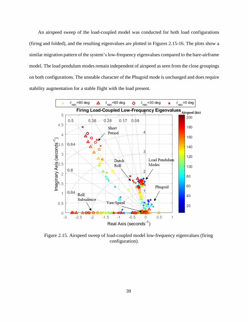
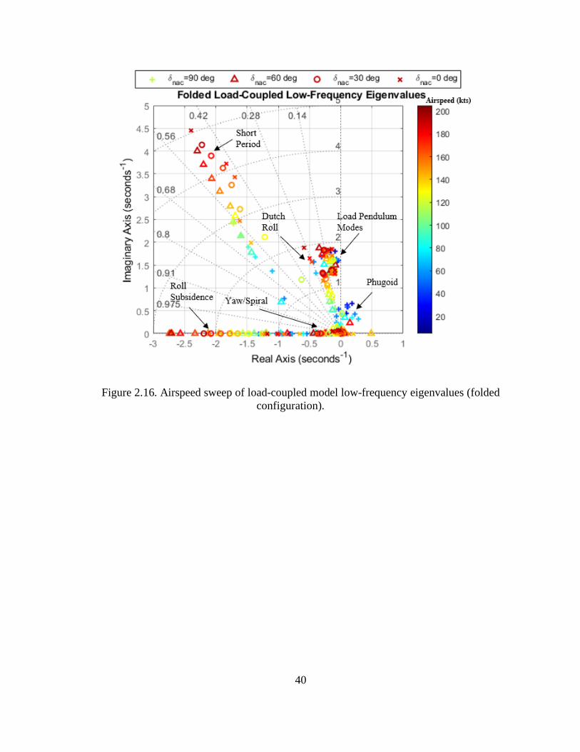
An airspeed sweep of the load-coupled model was conducted for both load configurations

(firing and folded), and the resulting eigenvalues are plotted in Figures 2.15-16. The plots show a

similar migration pattern of the system’s low-frequency eigenvalues compared to the bare-airframe

model. The load pendulum modes remain independent of airspeed as seen from the close groupings

on both configurations. The unstable character of the Phugoid mode is unchanged and does require

stability augmentation for a stable flight with the load present.

Figure 2.15. Airspeed sweep of load-coupled model low-frequency eigenvalues (firing

configuration).

40

Figure 2.16. Airspeed sweep of load-coupled model low-frequency eigenvalues (folded

configuration).

41

Chapter 3 Controller Design

3.1 Introduction

This chapter includes the controller design for active stabilization of the M119 external load

and the design of a SAS controller for the GTR model. The preliminary design of the ACH

controller for the M119 slung load applies classical control design methodology. The design uses

longitudinal and lateral cable angle feedback to damp longitudinal and lateral load pendulum

motions by translation of the active cargo hook. The preliminary design is based on tuning the

controller to achieve maximum load damping while meeting desired stability margins. The ACH

controller is a direct control mechanism that automatically varies the hook position to improve

load damping and system stability without pilot inputs. As described earlier, the idea of using

onboard active actuator control was examined in the past research for hover and low-speed flights

[22, 23], and demonstrated in flight [6]. The current paper focuses primarily on controller

performance during high-speed flights where the potential for load instability exists.

For the tiltrotor, a basic stability augmentation system is required to provide minimum

stability for the aircraft. Although the SAS design is not the focus of the research, it is needed for

the investigation of the effectiveness of the load stabilization. Unstable or barely stable aircraft

will perturb the performance of the ACH controller. The design of the SAS controller uses a linear-

quadratic regulator (LQR) to stabilize the rotorcraft.

42

3.2 Control Design for the Isolated Load

As mentioned previously, the slung load pendulum dynamics were obtained as linear models

identified from open-loop frequency sweep tests in the wind tunnel. Test results showed that the

cable angle response to ACH translation correlated highly with on-axis responses (𝜃𝑐/𝑥, 𝜙𝑐/𝑦)

and off-axis responses were negligible. The identified linear model parameters (𝐾, 𝑃

, 𝜔𝑃 , ∆𝑡) were

scheduled by airspeed due to the dependence of system dynamics on dynamic pressure.

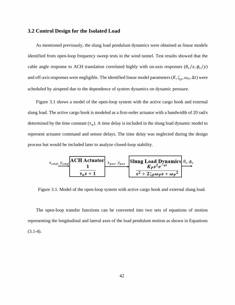
Figure 3.1 shows a model of the open-loop system with the active cargo hook and external

slung load. The active cargo hook is modeled as a first-order actuator with a bandwidth of 20 rad/s

determined by the time constant (𝜏𝑎). A time delay is included in the slung load dynamic model to

represent actuator command and sensor delays. The time delay was neglected during the design

process but would be included later to analyze closed-loop stability.

Figure 3.1. Model of the open-loop system with active cargo hook and external slung load.

The open-loop transfer functions can be converted into two sets of equations of motion

representing the longitudinal and lateral axes of the load pendulum motion as shown in Equations

(3.1-4).

43

𝜃�� + 2𝑃

𝜔𝑃𝜃�� + 𝜔𝑃2𝜃𝑐 = 𝐾𝑃��

(3.1)

𝜏𝑎 ∙ �� + 𝑥 = 𝑥𝑐𝑚𝑑(𝑡 − 𝜏) (3.2)

𝜙�� + 2𝑃

𝜔𝑃𝜙�� + 𝜔𝑃2𝜙𝑐 = 𝐾𝑃�� (3.3)

𝜏𝑎 ∙ �� + 𝑦 = 𝑦𝑐𝑚𝑑(𝑡 − 𝜏) (3.4)

It can be seen that cable angle motion is related to the acceleration of the cargo hook (��, ��) for

each axis. Tables 2.3-4 show that the damping of the load pendulum motion increases with airspeed,

especially for the lateral axis. As indicated earlier, at high airspeeds (greater than 122kt FS for the

firing configuration and 174 kt FS for the folded configuration), the non-linear behavior of the

load such as LCO could not be captured by the linearized models. However, it was assumed that

if the controller was designed for airspeeds where the load was lightly damped, then the same

controller would stabilize the load and prevent it from ever reaching the LCO in the unstable

regions. This was ultimately proven to be true in experiments as discussed in Chapter 4.

The load at the hover condition was selected to demonstrate the controller design approach

since it had the smallest damping ratio of any stable condition. The firing configuration was

selected as the primary configuration for controller design. However, the pendulum dynamics for

the firing and folded configurations are similar. The lateral axis controller design was considered

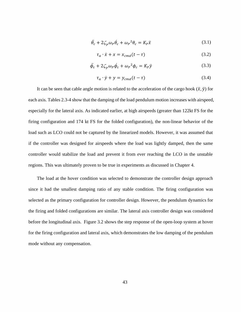
before the longitudinal axis. Figure 3.2 shows the step response of the open-loop system at hover

for the firing configuration and lateral axis, which demonstrates the low damping of the pendulum

mode without any compensation.

44

Figure 3.2. Open-loop simulation of lateral pendulum motion step response, (hover, firing

configuration).

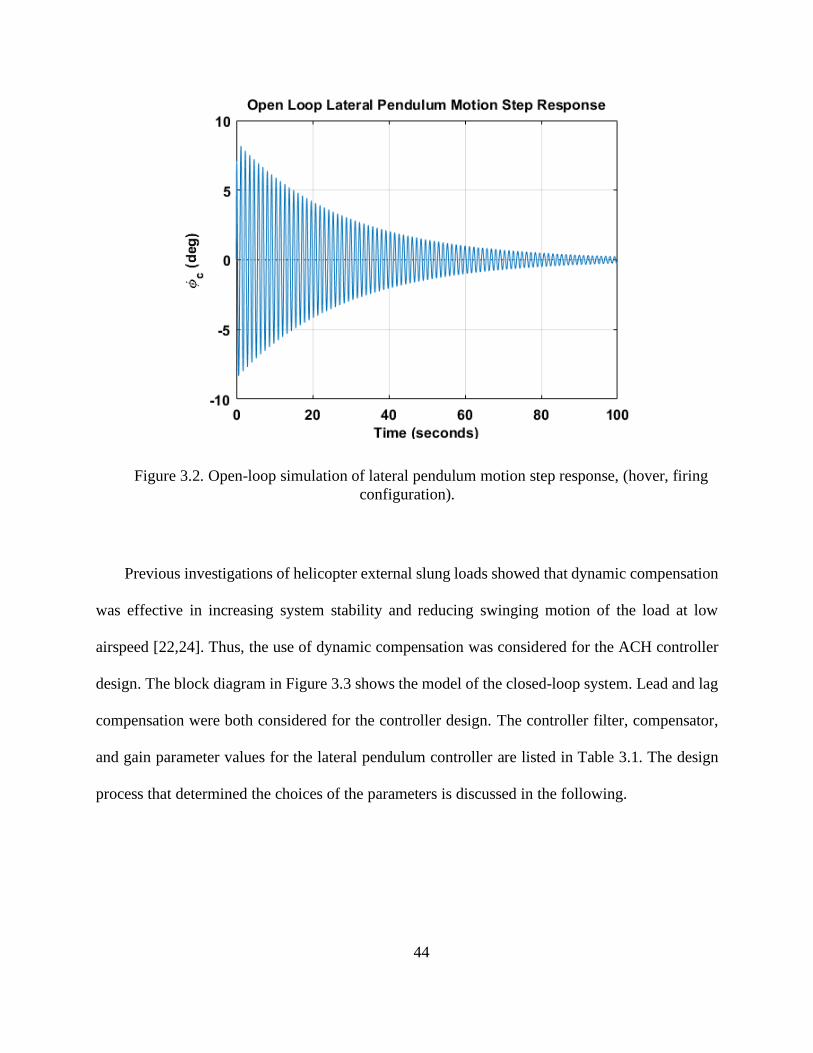
Previous investigations of helicopter external slung loads showed that dynamic compensation

was effective in increasing system stability and reducing swinging motion of the load at low

airspeed [22,24]. Thus, the use of dynamic compensation was considered for the ACH controller

design. The block diagram in Figure 3.3 shows the model of the closed-loop system. Lead and lag

compensation were both considered for the controller design. The controller filter, compensator,

and gain parameter values for the lateral pendulum controller are listed in Table 3.1. The design

process that determined the choices of the parameters is discussed in the following.

45

Figure 3.3. Block diagram of the closed-loop system.

Filter G(s) Compensator C(s) Gain K

Lead Design 1

s + p, p = 7.04

rad

s s −4.12,

mm

deg

Lag Design s

s + p, p = 0.1

rad

s

1

s + d, d = 1.85

rad

s 28.6,

mm

deg

Table 3.1. Controller parameters for the lateral pendulum mode (hover, firing configuration).

Using proportional derivative (PD) feedback has the benefit of improving system damping

and providing a quicker transient response. For the lead design, the controller transfer function is

composed by combining a pure derivative term (𝑠) and low pass filter (1

𝑠+𝑝), which is used to

decrease controller response to high-frequency disturbances to cable angle. The lead design uses

a negative gain value that shifts the phase of the output of the controller by 180 deg so that the

cargo hook motion is opposite in sign to the lateral cable angular rate.

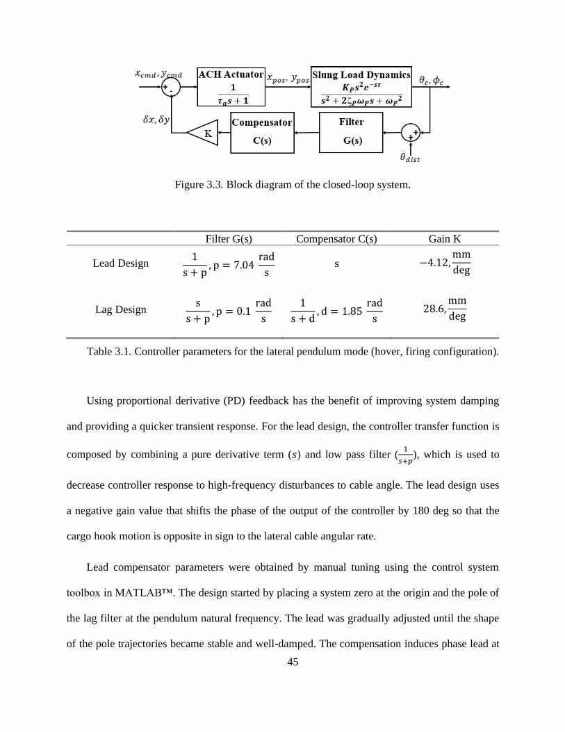
Lead compensator parameters were obtained by manual tuning using the control system

toolbox in MATLAB™. The design started by placing a system zero at the origin and the pole of

the lag filter at the pendulum natural frequency. The lead was gradually adjusted until the shape

of the pole trajectories became stable and well-damped. The compensation induces phase lead at

46

the resonance of the swinging load by driving the cargo hook to move in lead of the load response.

Figure 3.4 shows the root locus plot of the closed-loop system with the lead design. The closed-

loop pole trajectories of the pendulum mode shift toward the left of the s-plane, thus improving

system stability and damping. However, the closed-loop system now has an extra set of poles due

to the mixing of the actuator and the low pass filter that could shift to the unstable region when the

gain is high.

Figure 3.4. Root locus plot of the lateral pendulum mode with lead compensation, (hover,

firing configuration).

The broken loop frequency response in Figure 3.5 shows two sets of phase margins occurring

at two different gain crossover frequencies. The smallest between the two will be selected as the

minimum margin. The delay margin (DM) indicates the tolerance of the system towards time delay

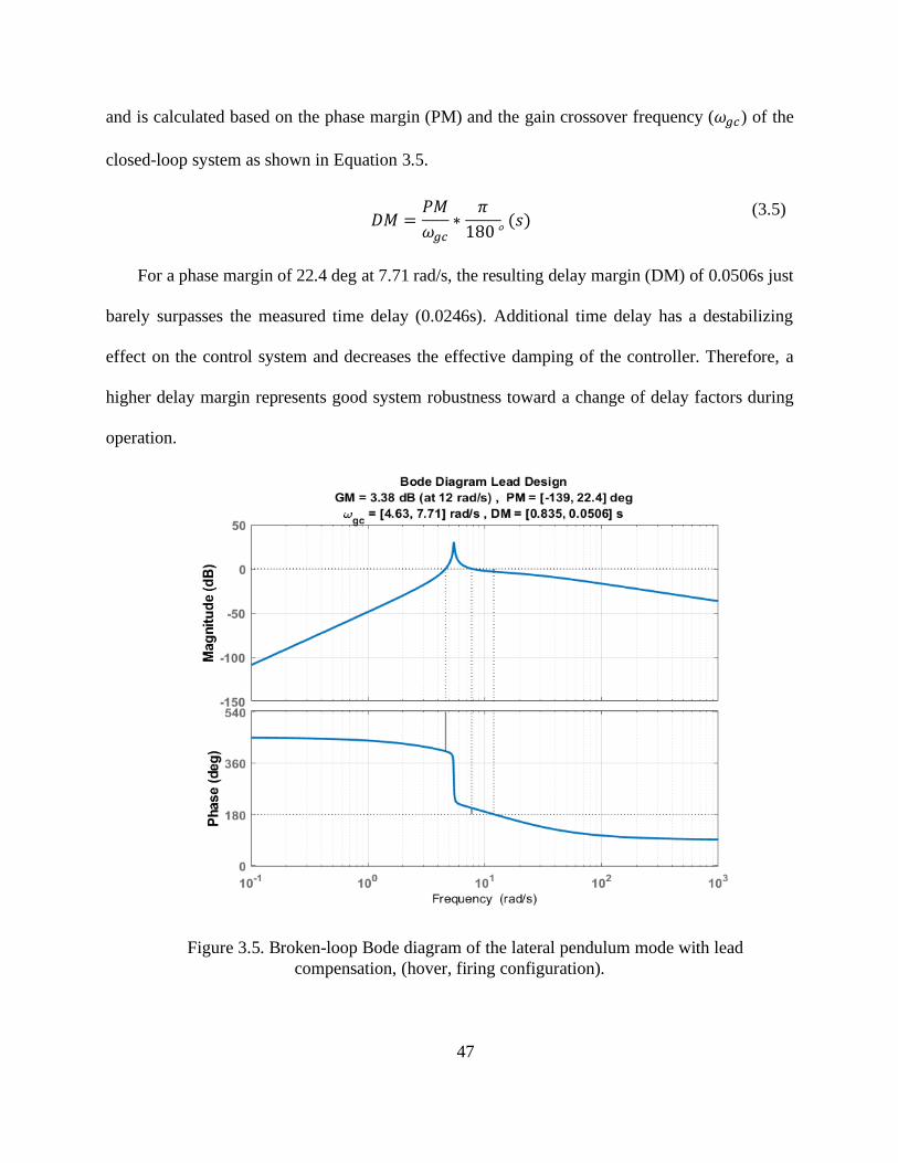
47

and is calculated based on the phase margin (PM) and the gain crossover frequency (𝜔𝑔𝑐) of the

closed-loop system as shown in Equation 3.5.

𝐷𝑀 =

𝑃𝑀

𝜔𝑔𝑐∗

𝜋

180° (𝑠)

(3.5)

For a phase margin of 22.4 deg at 7.71 rad/s, the resulting delay margin (DM) of 0.0506s just

barely surpasses the measured time delay (0.0246s). Additional time delay has a destabilizing

effect on the control system and decreases the effective damping of the controller. Therefore, a

higher delay margin represents good system robustness toward a change of delay factors during

operation.

Figure 3.5. Broken-loop Bode diagram of the lateral pendulum mode with lead

compensation, (hover, firing configuration).

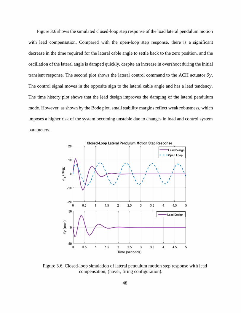
48

Figure 3.6 shows the simulated closed-loop step response of the load lateral pendulum motion

with lead compensation. Compared with the open-loop step response, there is a significant

decrease in the time required for the lateral cable angle to settle back to the zero position, and the

oscillation of the lateral angle is damped quickly, despite an increase in overshoot during the initial

transient response. The second plot shows the lateral control command to the ACH actuator 𝛿𝑦.

The control signal moves in the opposite sign to the lateral cable angle and has a lead tendency.

The time history plot shows that the lead design improves the damping of the lateral pendulum

mode. However, as shown by the Bode plot, small stability margins reflect weak robustness, which

imposes a higher risk of the system becoming unstable due to changes in load and control system

parameters.

Figure 3.6. Closed-loop simulation of lateral pendulum motion step response with lead


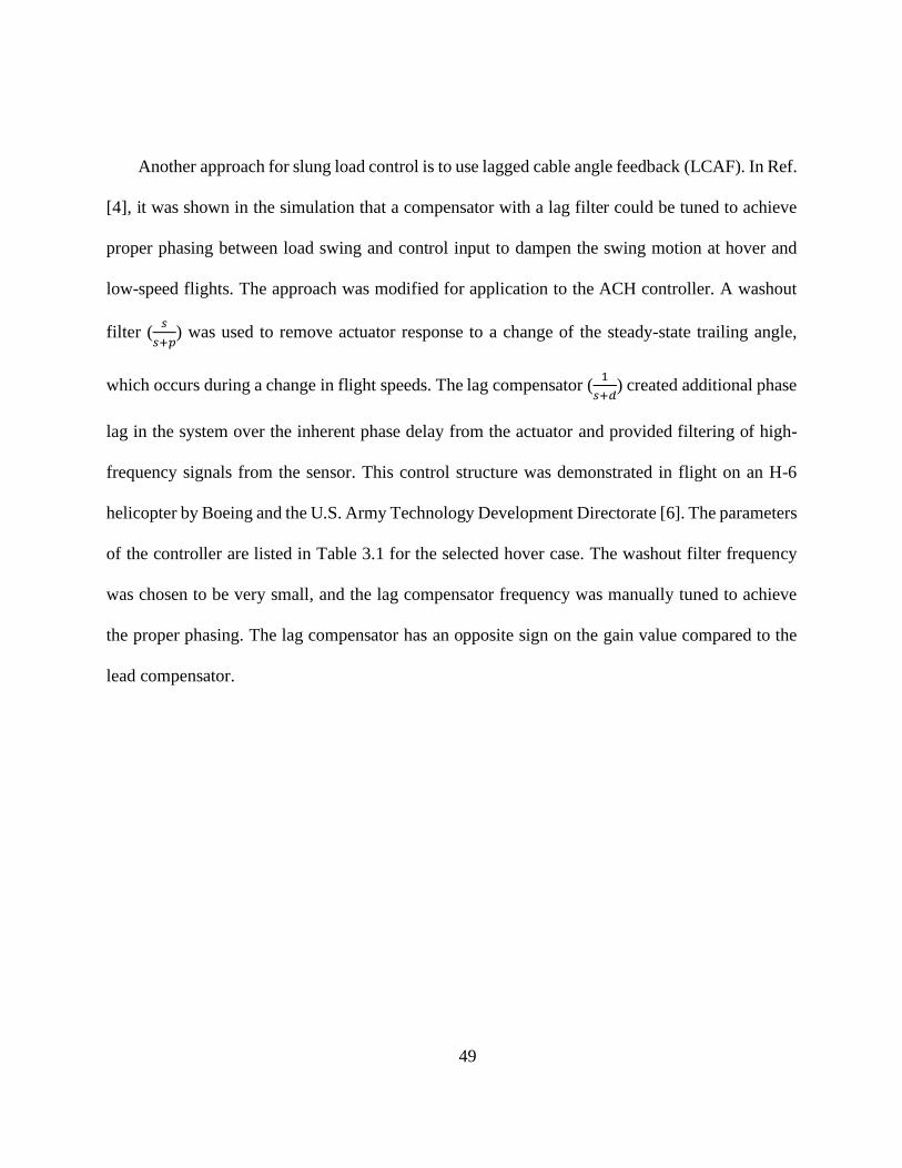
49

Another approach for slung load control is to use lagged cable angle feedback (LCAF). In Ref.

[4], it was shown in the simulation that a compensator with a lag filter could be tuned to achieve

proper phasing between load swing and control input to dampen the swing motion at hover and

low-speed flights. The approach was modified for application to the ACH controller. A washout

filter (𝑠

𝑠+𝑝) was used to remove actuator response to a change of the steady-state trailing angle,

which occurs during a change in flight speeds. The lag compensator (1

𝑠+𝑑) created additional phase

lag in the system over the inherent phase delay from the actuator and provided filtering of high-

frequency signals from the sensor. This control structure was demonstrated in flight on an H-6

helicopter by Boeing and the U.S. Army Technology Development Directorate [6]. The parameters

of the controller are listed in Table 3.1 for the selected hover case. The washout filter frequency

was chosen to be very small, and the lag compensator frequency was manually tuned to achieve

the proper phasing. The lag compensator has an opposite sign on the gain value compared to the

lead compensator.

50

Figure 3.7. Root locus plot of the lateral pendulum mode with lag compensation, (hover,

firing configuration).

The root locus plot for the lag design (Figure 3.7) shows better damping compared to the lead

design and all the closed-loop trajectories are in the stable region. The broken-loop response

(Figure 3.8) shows significant increases in the gain margin and phase margin as compared to the

lead design. The minimum delay margin of 0.1755 s also increases significantly and is well above

the measured time delay of the identified linear model (0.0246 s). The negative phase margin

indicates that the closed-loop system can be unstable if phase lead is added to the system around

the corresponding gain crossover frequency. This is reasonable as the controller is intentionally

adding phase lag to phase the control response to the swinging load.

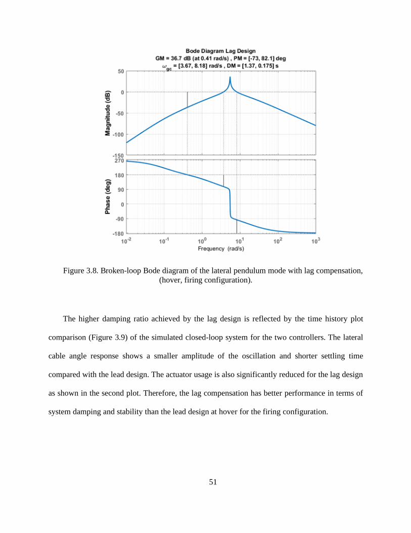
51

Figure 3.8. Broken-loop Bode diagram of the lateral pendulum mode with lag compensation,

(hover, firing configuration).

The higher damping ratio achieved by the lag design is reflected by the time history plot

comparison (Figure 3.9) of the simulated closed-loop system for the two controllers. The lateral

cable angle response shows a smaller amplitude of the oscillation and shorter settling time

compared with the lead design. The actuator usage is also significantly reduced for the lag design

as shown in the second plot. Therefore, the lag compensation has better performance in terms of

system damping and stability than the lead design at hover for the firing configuration.

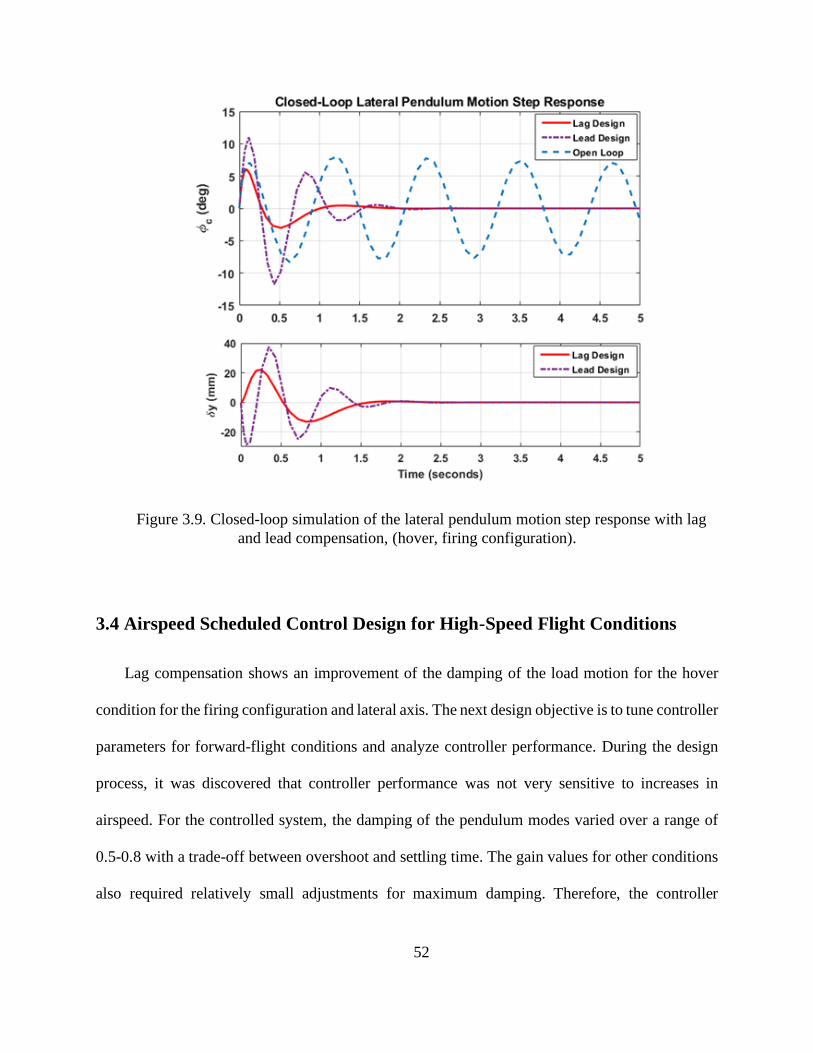
52


and lead compensation, (hover, firing configuration).

3.4 Airspeed Scheduled Control Design for High-Speed Flight Conditions

Lag compensation shows an improvement of the damping of the load motion for the hover

condition for the firing configuration and lateral axis. The next design objective is to tune controller

parameters for forward-flight conditions and analyze controller performance. During the design

process, it was discovered that controller performance was not very sensitive to increases in

airspeed. For the controlled system, the damping of the pendulum modes varied over a range of

0.5-0.8 with a trade-off between overshoot and settling time. The gain values for other conditions

also required relatively small adjustments for maximum damping. Therefore, the controller

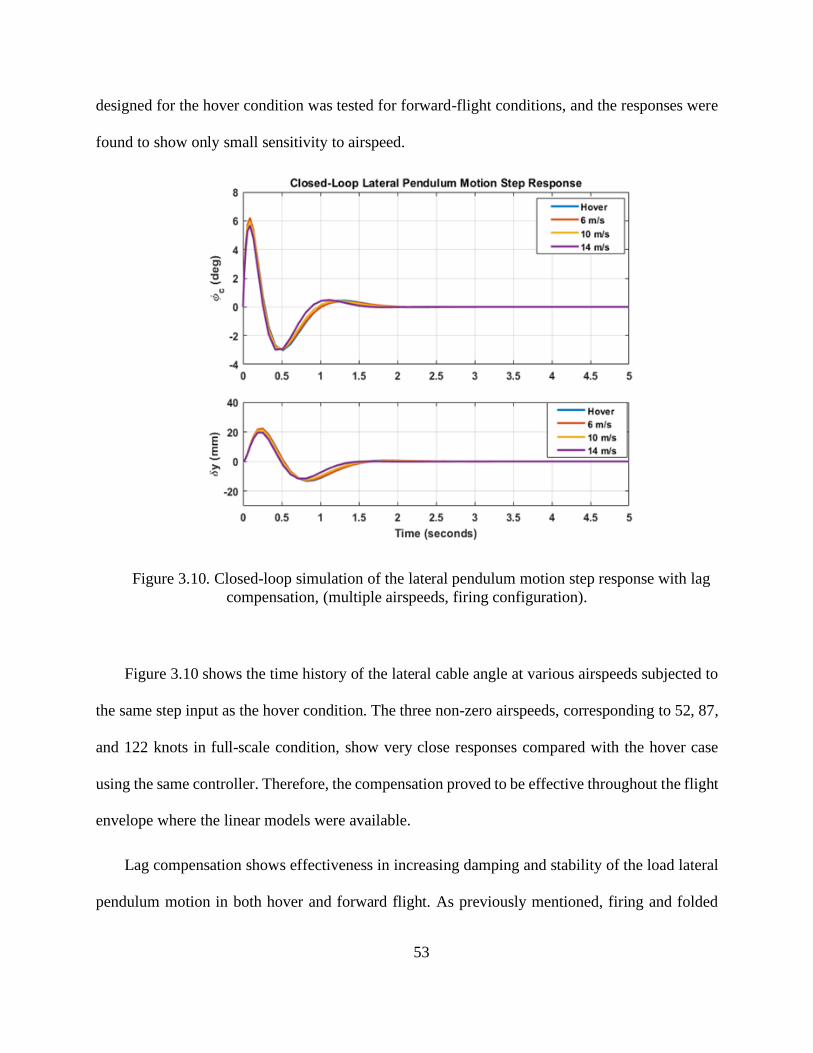
53

designed for the hover condition was tested for forward-flight conditions, and the responses were

found to show only small sensitivity to airspeed.


compensation, (multiple airspeeds, firing configuration).

Figure 3.10 shows the time history of the lateral cable angle at various airspeeds subjected to

the same step input as the hover condition. The three non-zero airspeeds, corresponding to 52, 87,

and 122 knots in full-scale condition, show very close responses compared with the hover case

using the same controller. Therefore, the compensation proved to be effective throughout the flight

envelope where the linear models were available.

Lag compensation shows effectiveness in increasing damping and stability of the load lateral

pendulum motion in both hover and forward flight. As previously mentioned, firing and folded

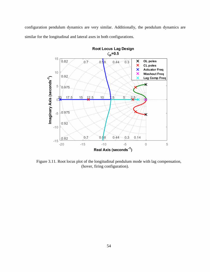
54

configuration pendulum dynamics are very similar. Additionally, the pendulum dynamics are

similar for the longitudinal and lateral axes in both configurations.

Figure 3.11. Root locus plot of the longitudinal pendulum mode with lag compensation,

(hover, firing configuration).

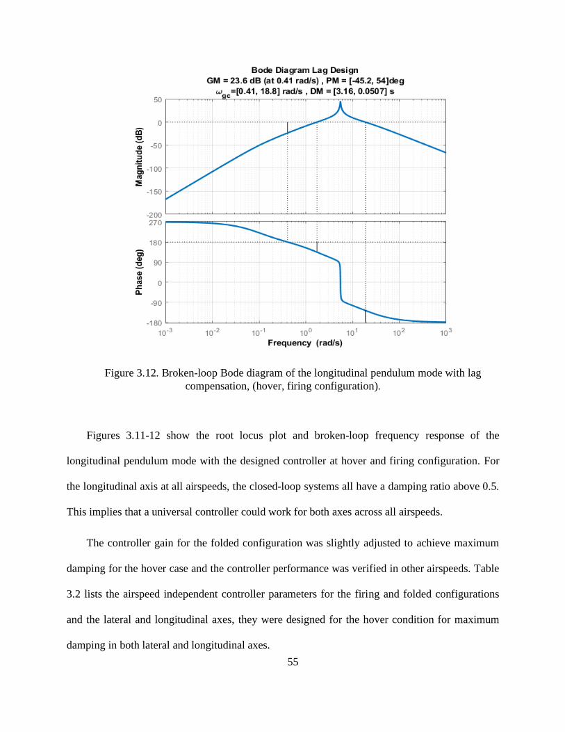
55

Figure 3.12. Broken-loop Bode diagram of the longitudinal pendulum mode with lag


Figures 3.11-12 show the root locus plot and broken-loop frequency response of the

longitudinal pendulum mode with the designed controller at hover and firing configuration. For

the longitudinal axis at all airspeeds, the closed-loop systems all have a damping ratio above 0.5.

This implies that a universal controller could work for both axes across all airspeeds.

The controller gain for the folded configuration was slightly adjusted to achieve maximum

damping for the hover case and the controller performance was verified in other airspeeds. Table

3.2 lists the airspeed independent controller parameters for the firing and folded configurations

and the lateral and longitudinal axes, they were designed for the hover condition for maximum

damping in both lateral and longitudinal axes.

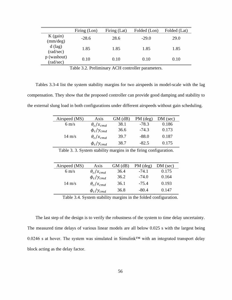
56

Firing (Lon) Firing (Lat) Folded (Lon) Folded (Lat)

K (gain)

(mm/deg) -28.6 28.6 -29.0 29.0

d (lag)

(rad/sec) 1.85 1.85 1.85 1.85

p (washout)

(rad/sec) 0.10 0.10 0.10 0.10

Table 3.2. Preliminary ACH controller parameters.

Tables 3.3-4 list the system stability margins for two airspeeds in model-scale with the lag

compensation. They show that the proposed controller can provide good damping and stability to

the external slung load in both configurations under different airspeeds without gain scheduling.

Airspeed (MS) Axis GM (dB) PM (deg) DM (sec)

6 m/s 𝜃𝑐/𝑥𝑐𝑚𝑑 38.1 -78.3 0.186

𝜙𝑐/𝑦𝑐𝑚𝑑 36.6 -74.3 0.173

14 m/s 𝜃𝑐/𝑥𝑐𝑚𝑑 39.7 -88.0 0.187

𝜙𝑐/𝑦𝑐𝑚𝑑 38.7 -82.5 0.175

Table 3. 3. System stability margins in the firing configuration.

Airspeed (MS) Axis GM (dB) PM (deg) DM (sec)

6 m/s 𝜃𝑐/𝑥𝑐𝑚𝑑 36.4 -74.1 0.175

𝜙𝑐/𝑦𝑐𝑚𝑑 36.2 -74.0 0.164

14 m/s 𝜃𝑐/𝑥𝑐𝑚𝑑 36.1 -75.4 0.193

𝜙𝑐/𝑦𝑐𝑚𝑑 36.8 -80.4 0.147

Table 3.4. System stability margins in the folded configuration.

The last step of the design is to verify the robustness of the system to time delay uncertainty.

The measured time delays of various linear models are all below 0.025 s with the largest being

0.0246 s at hover. The system was simulated in Simulink™ with an integrated transport delay

block acting as the delay factor.

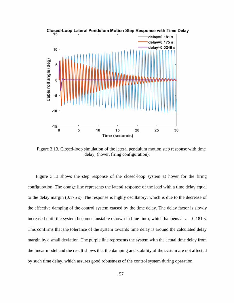
57

Figure 3.13. Closed-loop simulation of the lateral pendulum motion step response with time

delay, (hover, firing configuration).

Figure 3.13 shows the step response of the closed-loop system at hover for the firing

configuration. The orange line represents the lateral response of the load with a time delay equal

to the delay margin (0.175 s). The response is highly oscillatory, which is due to the decrease of

the effective damping of the control system caused by the time delay. The delay factor is slowly

increased until the system becomes unstable (shown in blue line), which happens at 𝜏 = 0.181 s.

This confirms that the tolerance of the system towards time delay is around the calculated delay

margin by a small deviation. The purple line represents the system with the actual time delay from

the linear model and the result shows that the damping and stability of the system are not affected

by such time delay, which assures good robustness of the control system during operation.

58

3.5 GTR Stability Augmentation System (SAS) Control Design

The linear analysis of the GTR model shows an unstable dynamic mode of the system at some

flight conditions. To test the effect of the designed ACH controller on the load-coupled model,

having a stable platform is required so that the performance of the controller would not be affected

by the instability of the aircraft. Considering most modern rotorcraft have onboard flight control

systems such as the AFCS (Automatic Flight Control System), which provides stability and

improves handling qualities of the aircraft, it is necessary to design a controller for the GTR model

for flight simulation.

Ref. [25] showed that using optimal control technique was an effective design for rotorcraft.

It demonstrated the design of an LQR (Linear Quadratic Regulator) on a generic non-linear

helicopter model and showed the success of improving the damping of the rotorcraft rigid body

modes and the advantages of using optimal controller design compared to conventional controllers.

For LQR problems, it requires to specify the weighting factors for the system states and the control

input [25]. The system is usually modeled as a state-space linear system as the following:

�� = 𝐴�� + 𝐵�� (3.6)

�� = 𝐶�� + 𝐷�� (3.7)

A gain matrix K that gives the optimal feedback control vector needs to be determined:

𝑢𝑓𝑏 = −𝐾�� (3.8)

Such that the result of the cost function shown below is minimized [25]:

𝐽 =

1

2∫ [��𝑇𝑄�� + ��𝑇𝑅��]𝑑𝑡

𝑡𝑓

0

(3.9)

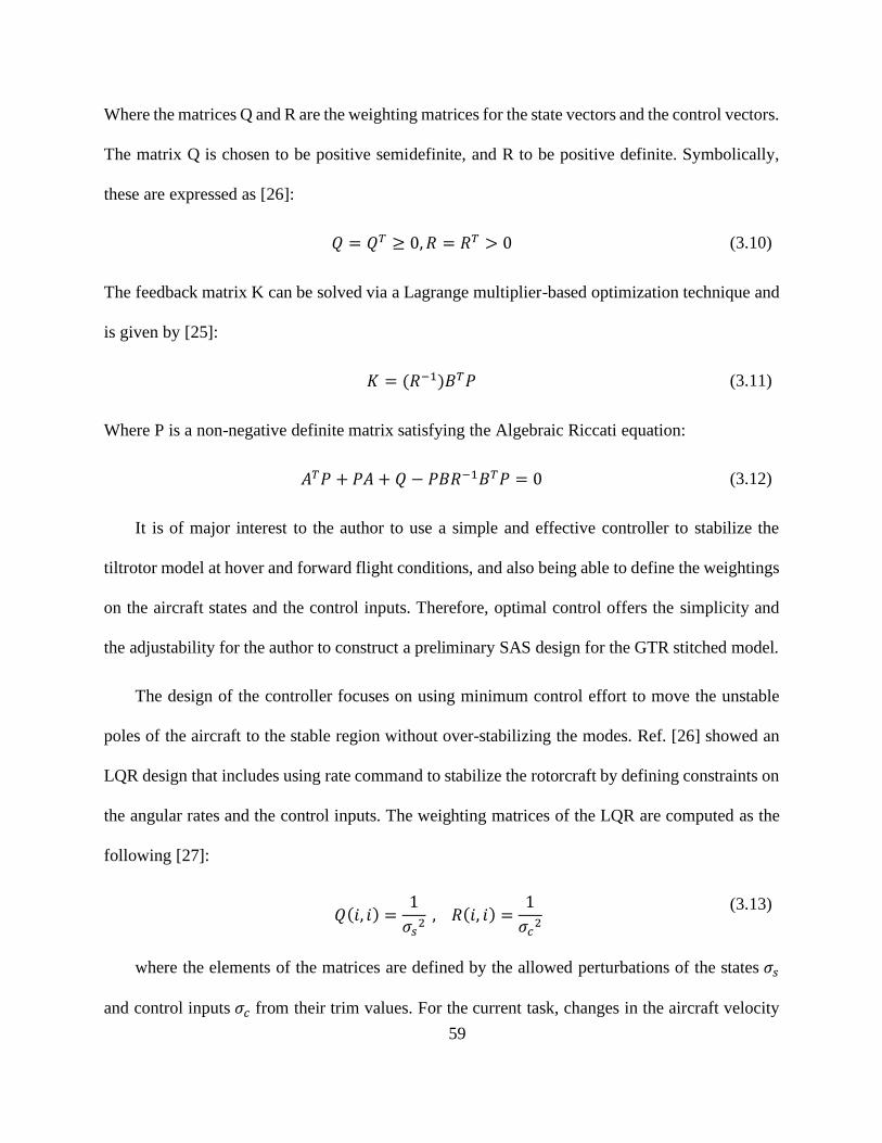
59

Where the matrices Q and R are the weighting matrices for the state vectors and the control vectors.

The matrix Q is chosen to be positive semidefinite, and R to be positive definite. Symbolically,

these are expressed as [26]:

𝑄 = 𝑄𝑇 ≥ 0, 𝑅 = 𝑅𝑇 > 0 (3.10)

The feedback matrix K can be solved via a Lagrange multiplier-based optimization technique and

is given by [25]:

𝐾 = (𝑅−1)𝐵𝑇𝑃 (3.11)

Where P is a non-negative definite matrix satisfying the Algebraic Riccati equation:

𝐴𝑇𝑃 + 𝑃𝐴 + 𝑄 − 𝑃𝐵𝑅−1𝐵𝑇𝑃 = 0 (3.12)

It is of major interest to the author to use a simple and effective controller to stabilize the

tiltrotor model at hover and forward flight conditions, and also being able to define the weightings

on the aircraft states and the control inputs. Therefore, optimal control offers the simplicity and

the adjustability for the author to construct a preliminary SAS design for the GTR stitched model.

The design of the controller focuses on using minimum control effort to move the unstable

poles of the aircraft to the stable region without over-stabilizing the modes. Ref. [26] showed an

LQR design that includes using rate command to stabilize the rotorcraft by defining constraints on

the angular rates and the control inputs. The weighting matrices of the LQR are computed as the

following [27]:

𝑄(𝑖, 𝑖) =

1

𝜎𝑠2

, 𝑅(𝑖, 𝑖) =1

𝜎𝑐2

(3.13)

where the elements of the matrices are defined by the allowed perturbations of the states 𝜎𝑠

and control inputs 𝜎𝑐 from their trim values. For the current task, changes in the aircraft velocity

60

and the attitude angles are not very important as the focus of the controller is to stabilize the aircraft

motion. Using rate command, the Q matrix is defined with constraints on the angular rates (p, q,

r) that have deviations equal to 30 deg/s, and the R matrix is defined with constrains on the 4

control inputs (𝑢𝑙𝑜𝑛,𝑢𝑙𝑎𝑡 , 𝑢𝑐𝑜𝑙, 𝑢𝑝𝑒𝑑 ) that have deviations equal to 10%. The SAS design was

conducted on the GTR bare-airframe model with the integrated control allocation module. The

designed gain matrix K is airspeed-scheduled from hover to 260 knots and is designed for multiple

nacelle angles at specific airspeeds in the conversion corridor. The SAS was integrated into the

load-coupled model.

Figure 3.14 plots the low-frequency eigenvalues of the system at hover and 120 knots forward

flight for firing configuration. At hover, the unstable Phugoid and Dutch Roll modes are stabilized

as the pole locations are moved to the left side of the imaginary axis. The effect of the SAS on the

load pendulum modes is not significant as the poles shift slightly from before. This is expected

since the stabilization of the rotorcraft prevents the energy exchange between the load and the

rotorcraft and the damping of the load motions through the aerodynamic damping provided by the

rotors. At forward flight, the unstable Phugoid mode is moved to the negative real axis, the

damping of the oscillatory modes such as the Short Period and the Dutch Roll modes are slightly

increased, and the other modes remain close to the positions before applying the SAS.

61

(a)

(b)

Figure 3.14. Eigenvalues of the load-coupled model (firing configuration) with the SAS

controller: (a) Hover, (b) 120 knots, 30° nacelle angle.

62

3.6 Control Design Conclusion

This chapter demonstrated the controller design process for the M119 isolated load and the

GTR bare-airframe model. For the M119 load, the design included two concepts (lead and lag

designs) that both used dynamic compensation to stabilize the load pendulum motion. Both designs

are proven to be able to increase the load damping across the tested speed range for both firing and

folded configurations. The lag design was chosen as it provides better stability margins, which

guarantees the close-loop system is more robust under the change of conditions. It was found that

a universal controller was able to increase the damping of the load pendulum motions in both the

longitudinal and lateral axis. The simulation results showed a close response of the load cable

angles across multiple airspeeds from hover to 122 knots while applying the same controller, and

it was expected that the load would be stabilized by such controller at higher airspeed where stable

linear load models were not able to be identified.

A SAS using an LQR controller was designed for the GTR bare-airframe model that provides

basic stability to the aircraft when the load is coupled. The SAS was able to stabilize the low-

frequency phugoid and Dutch-Roll modes by moving the poles of the system to the stable region

without over-stabilizing them. The eigenvalues of the load-coupled model showed that the SAS

has minimum effect on the load pendulum modes, which is important for isolating the control

effect of the SAS and the ACH controller on the load pendulum dynamics.

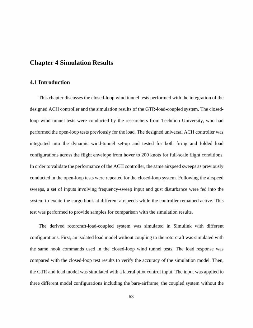
63

Chapter 4 Simulation Results

4.1 Introduction

This chapter discusses the closed-loop wind tunnel tests performed with the integration of the

designed ACH controller and the simulation results of the GTR-load-coupled system. The closed-

loop wind tunnel tests were conducted by the researchers from Technion University, who had

performed the open-loop tests previously for the load. The designed universal ACH controller was

integrated into the dynamic wind-tunnel set-up and tested for both firing and folded load

configurations across the flight envelope from hover to 200 knots for full-scale flight conditions.

In order to validate the performance of the ACH controller, the same airspeed sweeps as previously

conducted in the open-loop tests were repeated for the closed-loop system. Following the airspeed

sweeps, a set of inputs involving frequency-sweep input and gust disturbance were fed into the

system to excite the cargo hook at different airspeeds while the controller remained active. This

test was performed to provide samples for comparison with the simulation results.

The derived rotorcraft-load-coupled system was simulated in Simulink with different

configurations. First, an isolated load model without coupling to the rotorcraft was simulated with

the same hook commands used in the closed-loop wind tunnel tests. The load response was

compared with the closed-loop test results to verify the accuracy of the simulation model. Then,

the GTR and load model was simulated with a lateral pilot control input. The input was applied to

three different model configurations including the bare-airframe, the coupled system without the

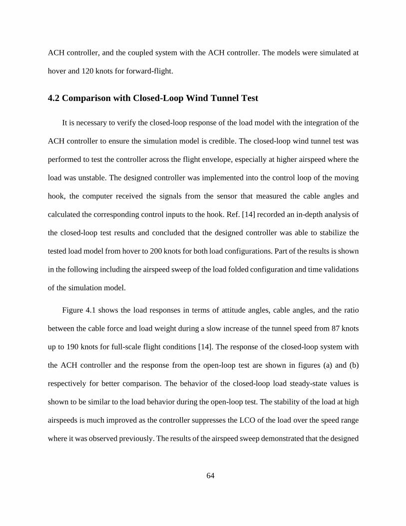
64

ACH controller, and the coupled system with the ACH controller. The models were simulated at

hover and 120 knots for forward-flight.

4.2 Comparison with Closed-Loop Wind Tunnel Test

It is necessary to verify the closed-loop response of the load model with the integration of the

ACH controller to ensure the simulation model is credible. The closed-loop wind tunnel test was

performed to test the controller across the flight envelope, especially at higher airspeed where the

load was unstable. The designed controller was implemented into the control loop of the moving

hook, the computer received the signals from the sensor that measured the cable angles and

calculated the corresponding control inputs to the hook. Ref. [14] recorded an in-depth analysis of

the closed-loop test results and concluded that the designed controller was able to stabilize the

tested load model from hover to 200 knots for both load configurations. Part of the results is shown

in the following including the airspeed sweep of the load folded configuration and time validations

of the simulation model.

Figure 4.1 shows the load responses in terms of attitude angles, cable angles, and the ratio

between the cable force and load weight during a slow increase of the tunnel speed from 87 knots

up to 190 knots for full-scale flight conditions [14]. The response of the closed-loop system with

the ACH controller and the response from the open-loop test are shown in figures (a) and (b)

respectively for better comparison. The behavior of the closed-loop load steady-state values is

shown to be similar to the load behavior during the open-loop test. The stability of the load at high

airspeeds is much improved as the controller suppresses the LCO of the load over the speed range

where it was observed previously. The results of the airspeed sweep demonstrated that the designed

65

controller was able to stabilize the load at a speed range higher than the maximum speed from the

identified linear models.

(a) (b)

Figure 4.1. (a): Closed-loop system load response to increasing wind-tunnel speed with the

ACH controller (folded configuration) (from [19]). (b): Open-loop system load response to

increasing wind-tunnel speed without the ACH controller (folded configuration) (from [14]).

Figure 4.2 shows the load firing configuration undergoing the same airspeed sweep procedure

from 87 knots to 165 knots for full-scale flight conditions. The maximum tunnel speed was lower

than the folded configuration due to the reason that the load longitudinal trailing angel exceeded

42 degrees, which was close to the predetermined safety limit of 45 degree [14]. The controller

tested for the firing configuration was slightly modified in order to test the optimized version of

the ACH controller derived by TDD. The optimization was based on the preliminary designed

66

controller and the parameters of the controller were fine-tuned using the fight control design

software CONDUIT®, which uses a specification-driven optimization approach that enforces all

performance requirements with minimum actuator usage. The optimization procedure was

presented in Ref. [14] and will not be discussed here. Comparing the behavior of the load at firing

configuration with and without the ACH controller, the closed-loop system is shown to be much

more stable as the load responses remain close to their steady-state values at higher airspeeds,

where severe instability above 130 knots was observed during the open-loop tests. The preliminary

controller was also tested with the firing configuration and showed similar behavior as the

optimized controller [14].

Figure 4.2. (a): Closed-loop system load response to increasing wind-tunnel speed with the

ACH controller (firing configuration) (from [14]). (b): Open-loop system load response to

increasing wind-tunnel speed without the ACH controller (firing configuration) (from [14]).

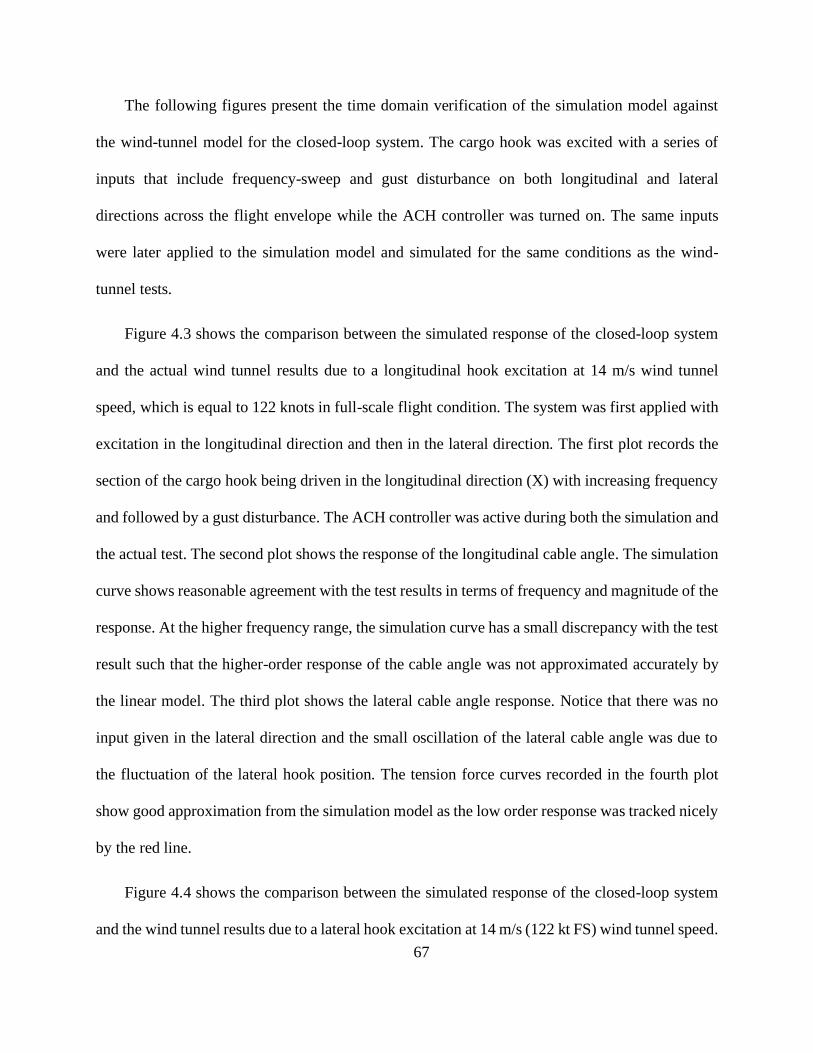
67

The following figures present the time domain verification of the simulation model against

the wind-tunnel model for the closed-loop system. The cargo hook was excited with a series of

inputs that include frequency-sweep and gust disturbance on both longitudinal and lateral

directions across the flight envelope while the ACH controller was turned on. The same inputs

were later applied to the simulation model and simulated for the same conditions as the wind-

tunnel tests.

Figure 4.3 shows the comparison between the simulated response of the closed-loop system

and the actual wind tunnel results due to a longitudinal hook excitation at 14 m/s wind tunnel

speed, which is equal to 122 knots in full-scale flight condition. The system was first applied with

excitation in the longitudinal direction and then in the lateral direction. The first plot records the

section of the cargo hook being driven in the longitudinal direction (X) with increasing frequency

and followed by a gust disturbance. The ACH controller was active during both the simulation and

the actual test. The second plot shows the response of the longitudinal cable angle. The simulation

curve shows reasonable agreement with the test results in terms of frequency and magnitude of the

response. At the higher frequency range, the simulation curve has a small discrepancy with the test

result such that the higher-order response of the cable angle was not approximated accurately by

the linear model. The third plot shows the lateral cable angle response. Notice that there was no

input given in the lateral direction and the small oscillation of the lateral cable angle was due to

the fluctuation of the lateral hook position. The tension force curves recorded in the fourth plot

show good approximation from the simulation model as the low order response was tracked nicely

by the red line.

Figure 4.4 shows the comparison between the simulated response of the closed-loop system

and the wind tunnel results due to a lateral hook excitation at 14 m/s (122 kt FS) wind tunnel speed.

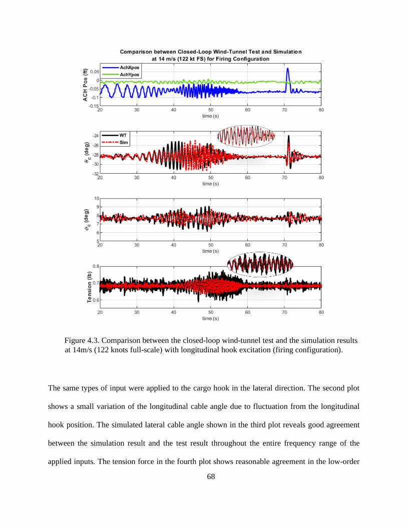
68

Figure 4.3. Comparison between the closed-loop wind-tunnel test and the simulation results

at 14m/s (122 knots full-scale) with longitudinal hook excitation (firing configuration).

The same types of input were applied to the cargo hook in the lateral direction. The second plot

shows a small variation of the longitudinal cable angle due to fluctuation from the longitudinal

hook position. The simulated lateral cable angle shown in the third plot reveals good agreement

between the simulation result and the test result throughout the entire frequency range of the

applied inputs. The tension force in the fourth plot shows reasonable agreement in the low-order

69

force dynamics. The spikes from the black line could represent the elastic modes that are not

captured by the low-order linear model.

Figure 4.4. Comparison between the closed-loop wind-tunnel test and the simulation results

at 14m/s (122 knots full-scale) with lateral hook excitation (firing configuration).

The comparison test was also performed at other airspeeds and the results showed credible

approximation to the simulation model. The comparison between the simulated result and the test

result verified that the simulation model was able to produce an approximate response of the load

70

due to the motion of the cargo hook. The ability of the designed ACH controller to stabilize the

load pendulum motions at high airspeeds was proven by the closed-loop wind tunnel tests as well

as by the simulation results.

4.3 GTR-Load Coupled System Simulation Results

Following the time domain validation of the simulation model, the GTR-load-coupled system

was simulated with a lateral pilot input to observe the behavior of the coupled system with and

without the controller. The models are simulated with three configurations including the bare-

airframe, the load-coupled airframe without the controller, and the load-coupled airframe with the

controller. Results of the simulation are shown for three different airspeeds that include 120 knots,

87 knots, and hover for full-scale fight conditions. The SAS was turned on throughout the entire

simulation process.

4.3.1 Simulation at 120 knots

This section shows the simulation results of the load-coupled system operating at 120 knots

with a nacelle angle of 30 deg. This speed approaches the envelope of high-speed slung load

carriage and it is also the highest airspeed where a linear load model could be identified. The

system was first simulated with a +/-30% lateral stick doublet input that was initiated at 3 seconds

after the start of the simulation. Figure 4.5 shows the response of the aircraft attitude angles for

the three configurations subjected to the same lateral input. The black lines indicate the aircraft

responses when there was no load attached, and it shows that the aircraft was stable under the

excitation from the control input which was expected since the tiltrotor behaves like a fixed-wing

aircraft at such speed and is dynamically stable. The blue lines represent the aircraft response after

the load was attached and show clear oscillation of the aircraft roll and yaw angles. The aircraft

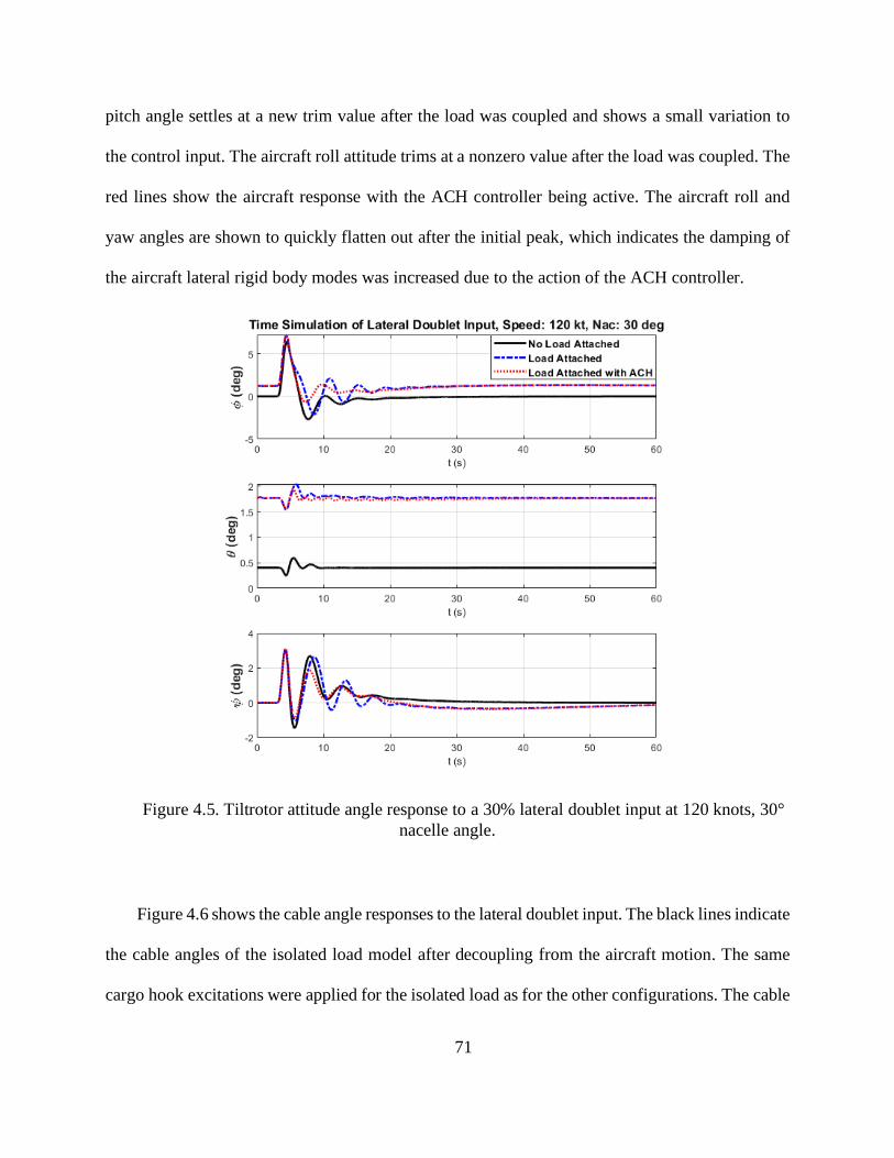
71

pitch angle settles at a new trim value after the load was coupled and shows a small variation to

the control input. The aircraft roll attitude trims at a nonzero value after the load was coupled. The

red lines show the aircraft response with the ACH controller being active. The aircraft roll and

yaw angles are shown to quickly flatten out after the initial peak, which indicates the damping of

the aircraft lateral rigid body modes was increased due to the action of the ACH controller.

Figure 4.5. Tiltrotor attitude angle response to a 30% lateral doublet input at 120 knots, 30°

nacelle angle.

Figure 4.6 shows the cable angle responses to the lateral doublet input. The black lines indicate

the cable angles of the isolated load model after decoupling from the aircraft motion. The same

cargo hook excitations were applied for the isolated load as for the other configurations. The cable

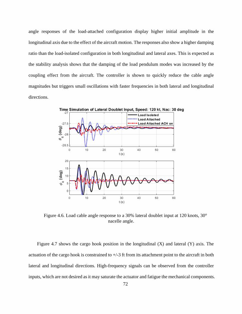
72

angle responses of the load-attached configuration display higher initial amplitude in the

longitudinal axis due to the effect of the aircraft motion. The responses also show a higher damping

ratio than the load-isolated configuration in both longitudinal and lateral axes. This is expected as

the stability analysis shows that the damping of the load pendulum modes was increased by the

coupling effect from the aircraft. The controller is shown to quickly reduce the cable angle

magnitudes but triggers small oscillations with faster frequencies in both lateral and longitudinal

directions.

Figure 4.6. Load cable angle response to a 30% lateral doublet input at 120 knots, 30°

nacelle angle.

Figure 4.7 shows the cargo hook position in the longitudinal (X) and lateral (Y) axis. The

actuation of the cargo hook is constrained to +/-3 ft from its attachment point to the aircraft in both

lateral and longitudinal directions. High-frequency signals can be observed from the controller

inputs, which are not desired as it may saturate the actuator and fatigue the mechanical components.

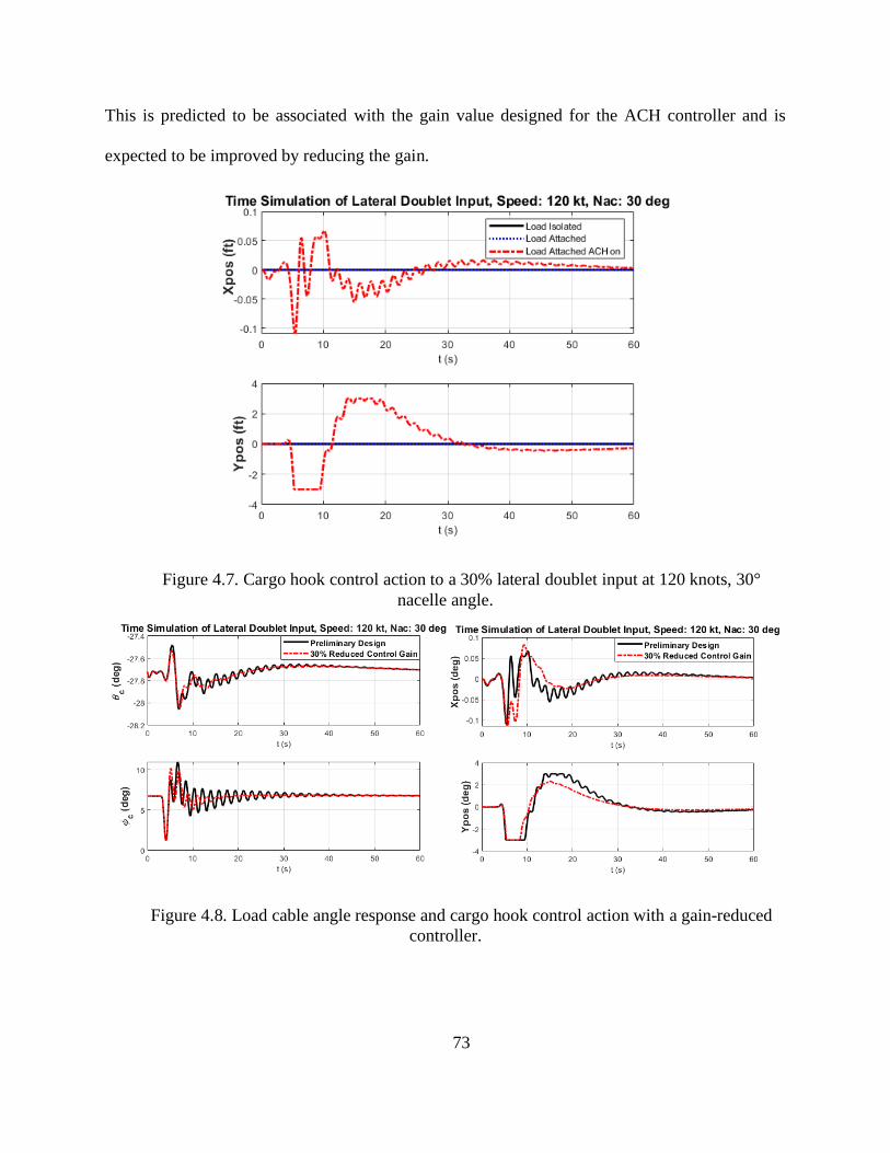
73

This is predicted to be associated with the gain value designed for the ACH controller and is

expected to be improved by reducing the gain.

Figure 4.7. Cargo hook control action to a 30% lateral doublet input at 120 knots, 30°

nacelle angle.

Figure 4.8. Load cable angle response and cargo hook control action with a gain-reduced

controller.

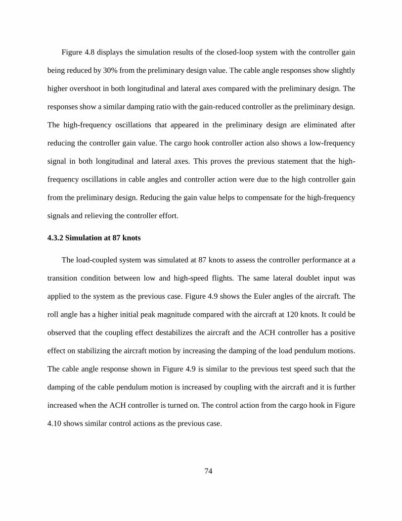
74

Figure 4.8 displays the simulation results of the closed-loop system with the controller gain

being reduced by 30% from the preliminary design value. The cable angle responses show slightly

higher overshoot in both longitudinal and lateral axes compared with the preliminary design. The

responses show a similar damping ratio with the gain-reduced controller as the preliminary design.

The high-frequency oscillations that appeared in the preliminary design are eliminated after

reducing the controller gain value. The cargo hook controller action also shows a low-frequency

signal in both longitudinal and lateral axes. This proves the previous statement that the high-

frequency oscillations in cable angles and controller action were due to the high controller gain

from the preliminary design. Reducing the gain value helps to compensate for the high-frequency

signals and relieving the controller effort.

4.3.2 Simulation at 87 knots

The load-coupled system was simulated at 87 knots to assess the controller performance at a

transition condition between low and high-speed flights. The same lateral doublet input was

applied to the system as the previous case. Figure 4.9 shows the Euler angles of the aircraft. The

roll angle has a higher initial peak magnitude compared with the aircraft at 120 knots. It could be

observed that the coupling effect destabilizes the aircraft and the ACH controller has a positive

effect on stabilizing the aircraft motion by increasing the damping of the load pendulum motions.

The cable angle response shown in Figure 4.9 is similar to the previous test speed such that the

damping of the cable pendulum motion is increased by coupling with the aircraft and it is further

increased when the ACH controller is turned on. The control action from the cargo hook in Figure

4.10 shows similar control actions as the previous case.

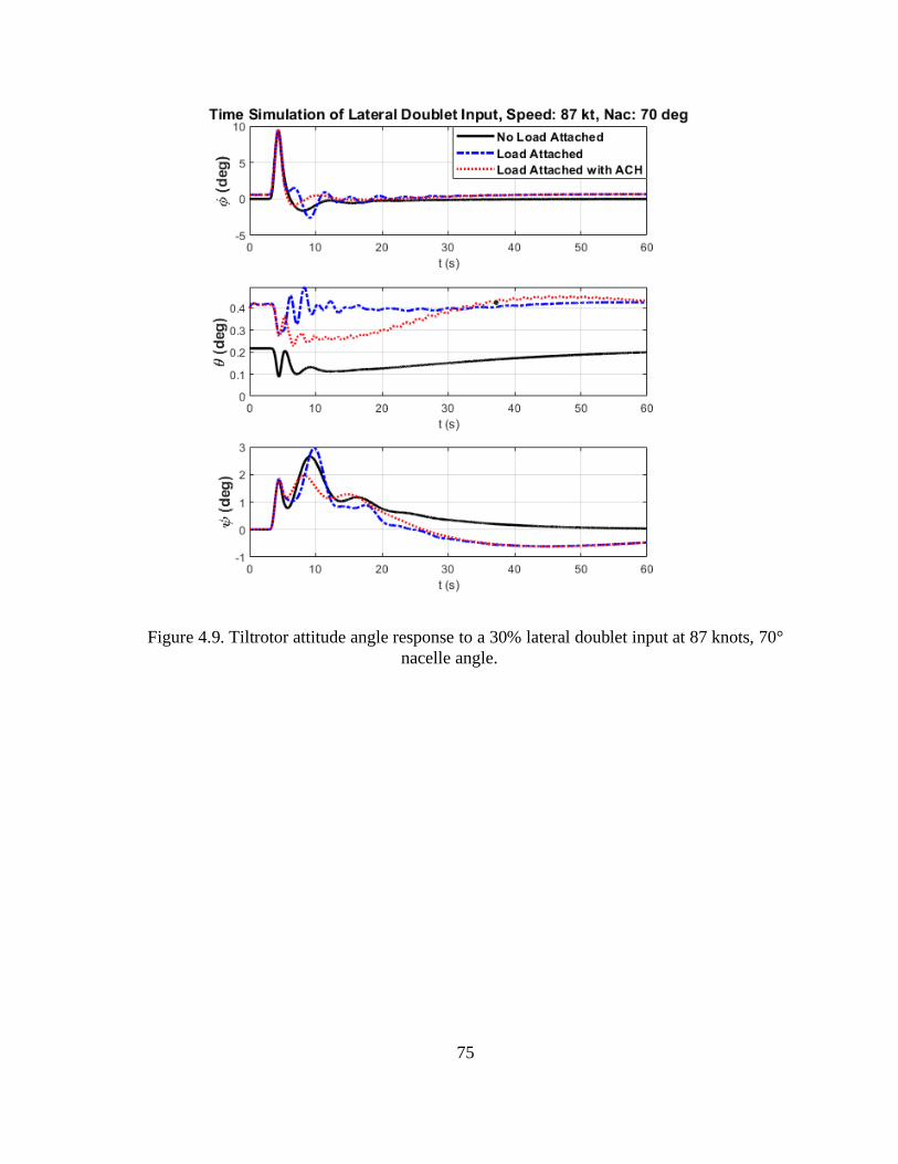
75


nacelle angle.

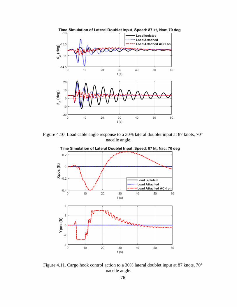
76

Figure 4.10. Load cable angle response to a 30% lateral doublet input at 87 knots, 70°

nacelle angle.

Figure 4.11. Cargo hook control action to a 30% lateral doublet input at 87 knots, 70°

nacelle angle.

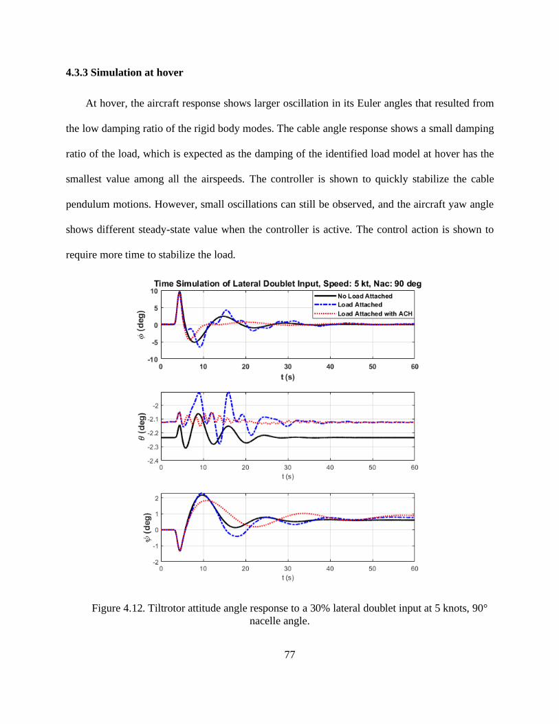
77

4.3.3 Simulation at hover

At hover, the aircraft response shows larger oscillation in its Euler angles that resulted from

the low damping ratio of the rigid body modes. The cable angle response shows a small damping

ratio of the load, which is expected as the damping of the identified load model at hover has the

smallest value among all the airspeeds. The controller is shown to quickly stabilize the cable

pendulum motions. However, small oscillations can still be observed, and the aircraft yaw angle

shows different steady-state value when the controller is active. The control action is shown to

require more time to stabilize the load.


nacelle angle.

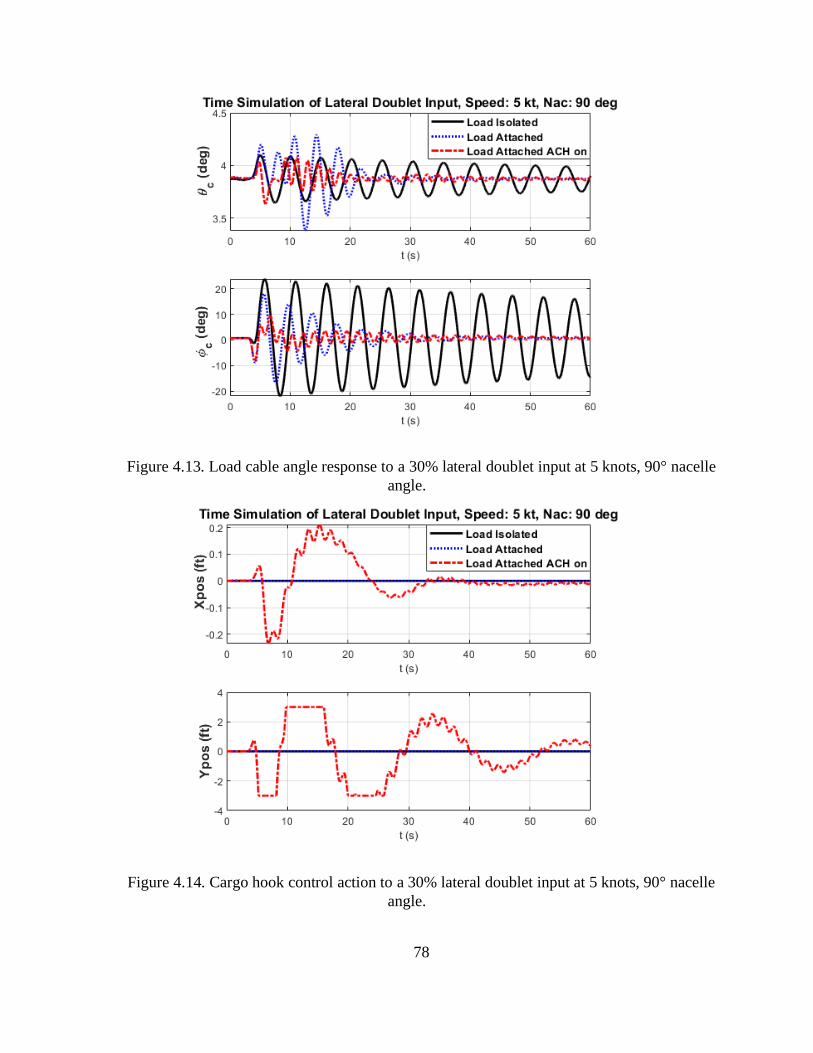
78


angle.

Figure 4.14. Cargo hook control action to a 30% lateral doublet input at 5 knots, 90° nacelle

angle.

79

4.3 Simulation Results Conclusions

The closed-loop wind tunnel test verified the performance of the controller as the load was

stabilized by the designed ACH across the flight envelope. The comparison of the test results with

the simulation results indicated a credible simulation model of estimating the linear dynamics of

the load system. For the GTR-load-coupled system, the ACH controller was then simulated at three

airspeeds with three different configurations. The coupled system appeared to have the highest

damping ratios of its rigid body modes and load pendulum modes when the ACH controller was

turned on. The designed ACH controller showed high-frequency input signals during stabilization

and caused small oscillations on the aircraft attitude angles and the load cable angles. This is

expected to be resolved after reducing the gain value of the controller. The target airspeed for the

system is 260 knots where the linear load model is not available. However, it is expected that the

designed ACH controller will remain effective up to the target speed, although it might require

modifications of control gain values in the future.

80

Chapter 5 Conclusions and Future Work

5.1 Conclusions

The thesis presents the study of using active stabilization method on a rotorcraft slung load

system consist of a generic tiltrotor (GTR) model and an M119 Howitzer. The objective of the

study was to design an ACH controller that can stabilize the load and extend the flight envelope

of the rotorcraft. The preliminary control design was based on the identified load pendulum

dynamics which were obtained from wind-tunnel testing and system identification conducted by

researchers from Technion University and U.S. Army TDD. The study also includes analysis of

the rotorcraft/load coupled system, simulation tests of the system with the integrated controller,

and verifications of the controller performance. The results from the study can be concluded as the

following:

1. Stability analysis of the GTR-load-coupled system shows that the coupling between the

load and the tiltrotor has a destabilizing effect on the rotorcraft rigid body modes and a stabilizing

effect on the load pendulum motions. This result agrees with past research of conventional

rotorcraft configurations. The stability analysis also shows unstable low-frequency eigenvalues of

the coupled system during low airspeeds. A SAS was designed to provide basic stability to the

tiltrotor bare-airframe to eliminate the effects of having an unstable aircraft platform on the overall

performance of the ACH controller. The designed SAS shows the ability to stabilize the tiltrotor

rigid-body modes without a significant impact on the load pendulum modes of the coupled-system.

81

2. Two ACH controllers were designed that both use dynamic compensation for load

stabilization. Both lead and lag designs show the ability to increase the damping of the load

pendulum motions. The lag design was chosen as it provides better stability margins and higher

damping for the closed-loop system. The controller design showed that a universal lag

compensator could be used to increase load damping across the flight envelope. The performance

of the designed controller was verified through closed-loop wind tunnel tests. The test results

showed stable load behavior from zero to 200 knots for full-scale flight conditions.

3. The simulation results of the isolated load model were compared with the closed-loop wind

tunnel tests with the integration of the designed ACH controller. Good agreements between the

simulation results and the test results are shown by the time domain validation of the closed-loop

system. The simulation model shows a good prediction of the load pendulum dynamics and

provides a reasonable approximation of the sling cable force dynamics.

4. From both simulation and wind tunnel results, the ACH controller was proved to be

effective in increasing load damping, minimizing LCO, and stabilizing the load pendulum motions

across the flight envelope from hover through 200 knots for full-scale conditions. The simulation

results also show high-frequency control inputs from the controller that resulted in small

oscillations in the tiltrotor attitude angles and load cable angles. It is shown that the problem was

associated with the high controller gain and can be resolved by reducing the gain value.

82

5.2 Future Work

For the current control design, future efforts should be put towards improving the controller

for real flight applications. One important aspect is the actuator constraints. This is because when

implementing the ACH device on an actual rotorcraft, the hook motion will be limited in both

range and speed depending on the size of the vehicle, which may cause saturation of the actuator

and degrade the performance of the controller. Therefore, studying the effects of the actuator

dynamics can help to understand the trade-offs between hook limitations and load stabilization.

Another important aspect is the handling qualities of the flight vehicle. Since the coupling effect

from the external load is destabilizing towards the rotorcraft, the vehicle’s handling qualities will

suffer degradation, which might lead to the demand for extra pilot workload or failure to satisfy

the requirement for specific carriage mission. This can be investigated by conducting a pilot-in-

the-loop flight simulation of the coupled system on a real-time flight simulator.

Other future research activities could involve developing a more advanced controller for load

stabilization. One example is to use both helicopter motion and ACH to stabilize the load, which

can address the problem of hook saturation due to a small stroke limit. Another example is to

design a MIMO controller which can be used to control both the helicopter and the load for

applications such as payload placement or package delivery using UAV.

83

Bibliography

[1] Raz, R., Rosen, A, Carmeli, A., Lusardi, J., Cicolani, L.S., Robinson, D., "Wind Tunnel and

Flight Evaluation of Passive Stabilization of a Cargo Container Slung Load", Journal of the

American Helicopter Society, Vol. 55, 03201, 2010, pp. 03200-1-18.

[2] Cicolani, L. S., Ivler, C., Ott, C., Raz, R. and Rosen, A., “Rotational Stabilization of Cargo

Container Slung Loads”, Journal of the American Helicopter Society, Vol.60, No.4, 2015,

042006-1-13.

[3] Ivler, C., “Design and Flight Test of a Cable Angle Feedback Control System for Improving

Helicopter Slung Load Operations at Low Speed,”

[4] Krishnamurthi, J., and Horn, J. F., "Helicopter Slung Load Control Using Lagged Cable Angle

Feedback," Journal of the American Helicopter Society, Vol. 60, (2), 2015, pp. 1-12. [5] Kang, K., Prasad, J. V. R., and Johnson E., “Active Control of a UAV Helicopter with a Slung

Load for Precision Airborne Cargo Delivery,” Journal of Unmanned Systems, Vol. 4, (3), 2016,

pp. 213-226. [6] Patterson, B. W., Ivler, C., Hayes, P. M., “External Load Stabilization Control Laws For An

H-6 Helicopter Testbed,” Proceedings of the 70th Annual Forum of the American Helicopter

Society, Montreal, Quebec, Canada, May 20-22, 2014.

[7] Enciu, J., Singh, A., and Horn, J. F.,” Stabilization of External Loads in High Speed Flight

Using an Active Cargo Hook,” 43rd European Rotorcraft Forum, Milan, Italy, September 12-

15, 2017.

[8] Singh, A., Enciu, J. and Horn, J. F., “Slung Load Stabilization Across the Flight Envelope

Using an Active Cargo Hook,” AIAA Scitech 2019 Forum, San Diego, California, 7-11

January 2019.

[9] Berger, T., “Handling Qualities Requirements and Control Design for High-Speed Rotorcraft,”

Ph.D. Thesis, Department of Aerospace Engineering, Pennsylvania State University,

University Park, 2019.

[10] Tobias, E. L. and Tischler, M. B., “A Model Stitching Architecture for Continuous Full Flight-

Envelope Simulation of Fixed-Wing Aircraft and Rotorcraft from Discrete-Point Linear

Models,” U.S. Army AMRDEC Special Report RDMR-AF-16-01, April 2016.

[11] “Multiservice Helicopter Sling Load: Single Point Rigging Procedures”, U. S. Department of

the Army TM 4-48.10, July, 2013.

[12] Wolowicz, H. C., Bowman, S. J. and Gilbert, P. W., “Similitude Requirements and Scaling

Relationships as Applied to Model Testing,” NASA Technical Paper 1435, Aug 1979.

[13] Islam, M., Jahra, F. and Hiscock, S., “Data Analysis Methodologies for Hydrodynamic

Experiments in Waves,” Journal of Naval Arichitecture and Matine Engineering, June 2016.

[14] Raz, R., Rosen, A, Nadell and J. S., Cicolani, L., Horn, F. J., Enciu, J., Chen, Z., Tischler, B.

M., Cheung, K. K., “Hardware-in-the-Loop Dynamic Wind Tunnel Investigation of Slung

84

Loads Dynamics with Application to Active Cargo Hook Stabilization of an M119 Howitzer,”

American Helicopter Society 76th Annual Forum, Oct 2020.

[15] Khalil, K. H., Nonlinear Systems, 3rd ed., Prentice Hall, Inc., 2002, Upper Saddle River, NJ.

[16] Tischler, M. B., Remple, R. K., Aircraft and Rotorcraft System Identification. 2nd ed.,

American Institute of Aeronautics and Astronautics, Inc., 2012, Reston, VA.

[17] “CIFER User’s Guide”, U.S. Army Aviation Development Directorate, Version 7.0.00

(Student).

[18] Juhasz, O., Celi, R., Ivler, C. M., Tischler, M. B., and Berger, T., “Flight Dynamic Simulation

Modeling of Large Flexible Tiltrotor Aircraft,” American Helicopter Society 68th Annual

Forum Proceedings, Fort Worth, TX, May 2012.

[19] Celi, R., “HeliUM 2 Flight Dynamic Simulation Model: Developments, Technical Concepts,

and Applications,” Proceedings of the 71st Annual Forum of the American Helicopter Society,

Virginia Beach, VA, May 2015.

[20] Ferguson, W. S., “A Methematical Model for Real Time Flight Simulation of A Generic Tilt-

Rotor Aircraft,” NASA Contractor Report, September 1988.

[21] Stevens, L. B., Lewis, L. F. and Johnson, N. E., Aircraft Control and Simulation: Dynamics,

Controls Design, and Autunomous Systems, John Wiley and Sons, Inc., 3rd ed., 2016,

Hoboken, NJ.

[22] Dukes, T. A., “Maneuvering Heavy Sling Loads near Hover, Part I: Damping the Pendulous

Motion,” Journal of the American Helicopter Society, Vol. 18,(3), 1973, pp. 2-11.

[23] Garnett, T.S., Jr., Smith, J.H., Lane, R., “Design and Flight Test of the Active Arm External

Load Stabilization System,” Proceedings of the American Helicopter Society 32nd Annual

Forum, Washington D.C., May 10-12, 1976.

[24] Bisgaard, M., la Cour-Harbo, A., and Bendsten J.D., “Swing Damping for Helicopter Slung

Load Systems Using Delayed Feedback,” AIAA Guidance, Navigation, & Control Conference,

Chicago, IL, August 10-13, 2009.

[25] Prasanna Raj, S., “Use of Optimal Control Technique in Design of AFCS Control Laws &

Way Ahead,” Rotary Wing Research & Design Centre, Bengaluru, India.

[26] Sinha, A., Linear Systems-Optimal and Robust Control, Tylor & Francis Group, LLC., 2007,

Boca Raton, FL.

[27] Bink, J. J., Sharf, I., van Gool, P. C. A. and Mulder, A. J., “Design of Stability Augmentation

System for Model Helicopter,” Proceedings of the 54th Annual Forum of the American

Helicopter Society, May 20, 2015.

Documents

ACTIVE STABILIZATION OF ROTORCRAFT EXTERNAL SLUNG …