Active Volume Models for 3D Medical Image Segmentation

Tian Shen1 Hongsheng Li1 Zhen Qian2 Xiaolei Huang1

1 Department of Computer Science & Engineering, Lehigh University, Bethlehem, PA 180152 Piedmont Heart Institute, Piedmont Healthcare, Atlanta, GA 30309

{tis207, h.li}@lehigh.edu, zhen.qian@piedmont.org, xih206@lehigh.edu

Abstract

In this paper, we propose a novel predictive model forobject boundary, which can integrate information from anysources. The model is a dynamic “object” model whosemanifestation includes a deformable surface representingshape, a volumetric interior carrying appearance statis-tics, and an embedded classifier that separates object frombackground based on current feature information. UnlikeSnakes, Level Set, Graph Cut, MRF and CRF approaches,the model is “self-contained” in that it does not model thebackground, but rather focuses on an accurate representa-tion of the foreground object’s attributes. As we will show,however, the model is capable of reasoning about the back-ground statistics thus can detect when is change sufficientto invoke a boundary decision. The shape of the 3D modelis considered as an elastic solid, with a simplex-mesh (i.e.finite element triangulation) surface made of thousands ofvertices. Deformations of the model are derived from a lin-ear system that encodes external forces from the boundaryof a Region of Interest (ROI), which is a binary mask rep-resenting the object region predicted by the current model.Efficient optimization and fast convergence of the model areachieved using the Finite Element Method (FEM). Otheradvantages of the model include the ease of dealing withtopology changes and its ability to incorporate human inter-actions. Segmentation and validation results are presentedfor experiments on noisy 3D medical images.

1. Introduction

Boundary extraction is an important task in image anal-ysis. The main challenge is to retrieve high-level infor-mation from low-level image signals while minimizing theeffect of noise, intensity inhomogeneity, and other factors.Model-based methods have been widely used with consid-erable success. Most noticeable are two types of models:deformable models [10, 14], and statistical shape and ap-pearance model [4, 5].

Kass et al. proposed Snakes [10], which are energy-

minimizing splines with smoothness constraints and influ-enced by image forces. Other parametric deformable mod-els were proposed to incorporate overall shape and motionconstraints [20, 16] and to increase the attraction range ofthe original Snakes by Gradient Vector Flow (GVF) [22].Depending solely on image gradient information, however,these methods may be trapped by noise and spurious edges.Region analysis strategies [24, 9, 7] have been incorporatedin Snake-like models to improve their robustness to noise.

Another class of deformable models is level set basedgeometric models [14, 7]. This approach representscurves and surfaces implicitly as the level set of a higher-dimensional scalar function and the evolution of these im-plicit models is based on the theory of curve evolution, withspeed function specifically designed to incorporate imagegradient information. The integration of region informationin geometric models has been mostly based on solving theframe partition problem as in Geodesic Active Region [17]and Active contours without edges [2]. The level-set mod-els are more computationally expensive and often requireknowing the number of regions and appearance statistics ofeach region a priori, but they are free in topology and do notneed explicit parameterization. So the level-set approachis commonly used in segmenting multiple objects [8] andachieves good result in tubular structure segmentation [21].Coupled surface constraints and dual-front implementationof level set active contours [13] also provide the flexibilityof capturing variable degrees of localness in optimization.

In noisy images, statistical modeling approaches can addconstraints from prior off-line learning. Cootes et al. pro-posed methods for building active shape models [5] and ac-tive appearance models [4], by learning patterns of vari-ability from a training set of annotated images. Integrat-ing high-level knowledge, these models deform in waysconstrained by the training data and are often more ro-bust in image interpretation. Image interpretation by shape-appearance joint prior models can be based on image search[5], or by maximizing posterior likelihood of the modelgiven image information, in a Bayesian framework [23].In medical imaging, shape priors particularly have beenintroduced to cardiac segmentation [11, 25], and to de-

1

formable models for constrained segmentation of bladderand prostate [6]. One limitation of the statistical models isin the laborious training data collection and annotation pro-cess.

In this paper, we propose a novel volumetric deformablemodel which we term the Active Volume Models (AVM).Compared with active contour and active shape/appearancemodels, the AVM is a “self-contained” generative objectmodel that does not require off-line training but generatesuseful priors about the object. It focuses on an accuratemodeling of the foreground object’s attributes and embodiesobject feature statistics learned adaptively as the model de-forms toward object boundary. With additional informationabout the overall image feature statistics, the model also es-timates the background statistics so that a Bayes classifiercan be applied to predicting dynamically the object region(Section 2.3). In its object-region prediction framework, themodel is capable of probabilistically integrating constraintsfrom multiple visual cues.

The AVM model’s shape is represented by a simplexmesh (or finite-element triangulation) and its volumetric in-terior carries the various visual appearance feature statis-tics. An advantage of the AVM formulation is that it al-lows the predicted object-region information to naturallybecome part of a linear system (Section 3.3), the solutionof which gives the deformation of the model to minimizean energy function designed to deform the model towardobject boundary.

Being a parametric model fitting approach, the AVMmodel convergence is fast, typically taking no more than40 iterations. Several factors contribute to this efficiency:(1) AVM focuses on modeling the foreground object andthen reason about the background, instead of modeling thebackground explicitly, (2) the model’s deformations can besolved in a linear system, and (3) multiple external con-straints are combined in a probabilistic framework and to-gether contribute to long-range forces coming directly fromthe predicted object region boundary. In our experimen-tal evaluation on various 3D noisy medical images, AVMdeforms much faster than level set methods such as Activecontours without edges(ACWE) [2]. Even though there arethousands of vertices (or nodes) on the surface of 3D AVM,the model’s deformation speed is still less than 20 secondsper iteration. The converged 3D AVM model is directlya smooth mesh representing the segmented object surface.Therefore it does not need any post-processing step such assurface reconstruction, as required by other methods includ-ing region growing, level set, graph cut and MRF.

The remainder of the paper is organized as follows. InSection 2, we introduce the representation and the bound-ary prediction module of 3D AVM. In Section 3, we presentthe deformation of AVM based on gradient and object re-gion information. In Section 4, experimental results are pre-sented. We conclude the paper and discuss future work in

Section 5.

2. The Active Volume Model

An AVM is a deforming solid that minimizes internaland external energy [19]. The internal constraint ensuresthe model has smooth boundary or surface. The externalconstraints come from image data, prior, and user definedfeatures. In this section, we introduce the representations of3D AVM, and introduce a novel object boundary predictionmodule by AVM.

2.1. Explicit Shape Representation of 3D AVM

The shape of a 2D AVM is defined similarly to activecontours [10], as a spline curve that has associated elasticityand rigidity. In 3D, the surface of a model can be definedby a mapping

Λ = [0, 1] × [0, 1] → R3

(s, r) → v(s, r) = (x(s, r), y(s, r), z(s, r)), (1)

and the model’s internal energy in 3D is defined as aSobolev smoothing term

Eint =∫Λ(α(s)|vs|2 + α(r)|vs|2 + β(s)|vss|2

+β(r)|vrr|2 + β(sr)|vsr|2)dsdr(2)

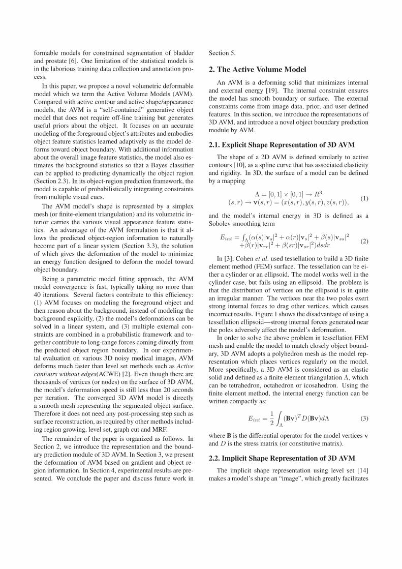
In [3], Cohen et al. used tessellation to build a 3D finiteelement method (FEM) surface. The tessellation can be ei-ther a cylinder or an ellipsoid. The model works well in thecylinder case, but fails using an ellipsoid. The problem isthat the distribution of vertices on the ellipsoid is in quitean irregular manner. The vertices near the two poles exertstrong internal forces to drag other vertices, which causesincorrect results. Figure 1 shows the disadvantage of using atessellation ellipsoid—strong internal forces generated nearthe poles adversely affect the model’s deformation.

In order to solve the above problem in tessellation FEMmesh and enable the model to match closely object bound-ary, 3D AVM adopts a polyhedron mesh as the model rep-resentation which places vertices regularly on the model.More specifically, a 3D AVM is considered as an elasticsolid and defined as a finite element triangulation Λ, whichcan be tetrahedron, octahedron or icosahedron. Using thefinite element method, the internal energy function can bewritten compactly as:

Eint =12

∫Λ

(Bv)T D(Bv)dΛ (3)

where B is the differential operator for the model vertices vand D is the stress matrix (or constitutive matrix).

2.2. Implicit Shape Representation of 3D AVM

The implicit shape representation using level set [14]makes a model’s shape an “image”, which greatly facilitates

(A)

(B)

(1) (2)Figure 1. Comparing heart Left Ventricle segmentation by tessel-lation and by triangulation models. (A) Tessellation model with400×120 vertices. Notice that the two poles exert very strongforce to drag other vertices which causes the incorrect result. (B)Finite Element Triangulation model with 40,962 vertices. (1)&(2)Two different views.

the integration of boundary and region information [9]. For3D AVM, we compute the implicit representation of modelshape to be used in region-based external energy terms. TheEuclidean distance transform is applied to embed implicitlyan evolving model’s surface in a higher dimensional dis-tance function. Let Φ : Ω → R+ be a Lipschitz functionthat refers to the distance transform for the model shape M.By definition Ω is bounded since it refers to the image do-main. The shape defines a partition of domain: the regionthat is enclosed by M, [RM], the background [Ω − RM],and on the model, [∂RM]. Given these definition the fol-lowing equation is considered:

ΦM(x) =

⎧⎨⎩

0, x ∈ ∂RM+ED(x,M) > 0, x ∈ RM−ED(x,M) < 0, x ∈ [Ω −RM]

(4)

where ED(x,M) refers to the minimum Euclidean dis-tance between the image pixel/voxel location x and themodel M.

2.3. AVM Model’s Boundary Prediction Module

Different from most of deformable models, one of thenovel features of AVM is its adaptive object boundary pre-diction scheme. The model alternates between two opera-tions: deform according to the current object boundary pre-diction, and predict according to current appearance statis-tics of the model. Using this on-line prediction mecha-nism, the expected object information updates automati-cally while the model deforms. And long-range externalforces are generated from the predicted object boundary toeffectively deform the model.

External constraints from any sources can be accountedby probabilistic integration. Let us consider that each con-straint corresponds to a probabilistic boundary predictionmodule, and it generates a confidence-rated probability mapto indicate the likelihood of a pixel being: +1 (object class),or -1 (non object class). Suppose we have n independent

external constraints derived from image information, thefeature used in the kth constraint is fk, L(x) denotes thelabel of a pixel x. Our approach to combining the multipleindependent modules is applying the Bayes rule in order toevaluate the final confidence rate:

Pr(L(x)|f1, f2, ..., fn)= (Pr(f1, f2, ..., fn|L(x))Pr(L(x))/(Pr(f1, f2, ..., fn))∝ Pr(f1|L(x))Pr(f2|L(x))...P r(fn|L(x))Pr(L(x))

(5)For each independent module, the probability

Pr(fk|L(x)) is estimated based on the AVM model’scurrent statistics about feature fk as well as the overallfeature statistics in the image. The derivation is as follows.

Pr(fk) = Pr(fk, L(x) = +1) + Pr(fk, L(x) = −1)= Pr(fk|L(x) = +1)Pr(L(x) = +1)

+Pr(fk|L(x) = −1)Pr(L(x) = −1) (6)

Assuming the current AVM model embodies priors learneddynamically about the foreground object, we approximatethe probabilistic distribution of feature fk in the object,Pr(fk|L(x) = +1), by the feature’s distribution in the cur-rent AVM model. The overall distribution of fk in the im-age, Pr(fk), is also known. Both probability density func-tions, Pr(fk|L(x) = +1) and Pr(fk), are estimated usinga nonparametric kernel-based density estimation method[9]. The p.d.fs are differentiable and can represent complexmulti-modal distributions. Therefore, we can now reasonabout the feature distribution in the background

Pr(fk|L(x) = −1) =Pr(fk) − Pr(fk|L(x) = +1)Pr(L(x) = +1)

Pr(L(x) = −1). (7)

The prior independent of image features, Pr(L(x)), inEquations 5 and 7 can be assumed uniform: Pr(L(x) =+1) = 0.5 and Pr(L(x) = −1) = 0.5. Spatially-varyingprior is another choice. For instance, a Gaussian distancemodel can be adopted so that pixels close to the AVM modelhave higher prior probability being part of the object.

Once the posterior probabilities Pr(L(x)|f1, f2, ..., fn)are estimated, we apply the Bayesian decision rule to ob-tain a binary map PB whose foreground represents thepredicted object region. That is, PB(x) = 1 (objectpixel) if Pr(L(x) = +1|f1, f2, ..., fn) ≥ Pr(L(x) =−1|f1, f2, ..., fn), and PB(x) = 0 otherwise. The proba-bility of error for the decision at pixel x is min(Pr(L(x) =+1|f1, f2, ..., fn), P r(L(x) = −1|f1, f2, ..., fn)).

In this paper, we show that by considering two typesof features—pixel intensity i(x) and pixel gradient magni-tude g(x), and assuming a uniform prior for Pr(L(x)), theabove framework generates reasonable estimates of back-ground feature statistics (Equation 7) and consistently givesgood predictions of the object region on a variety of medicalimages.

(A)

(B)

(C)

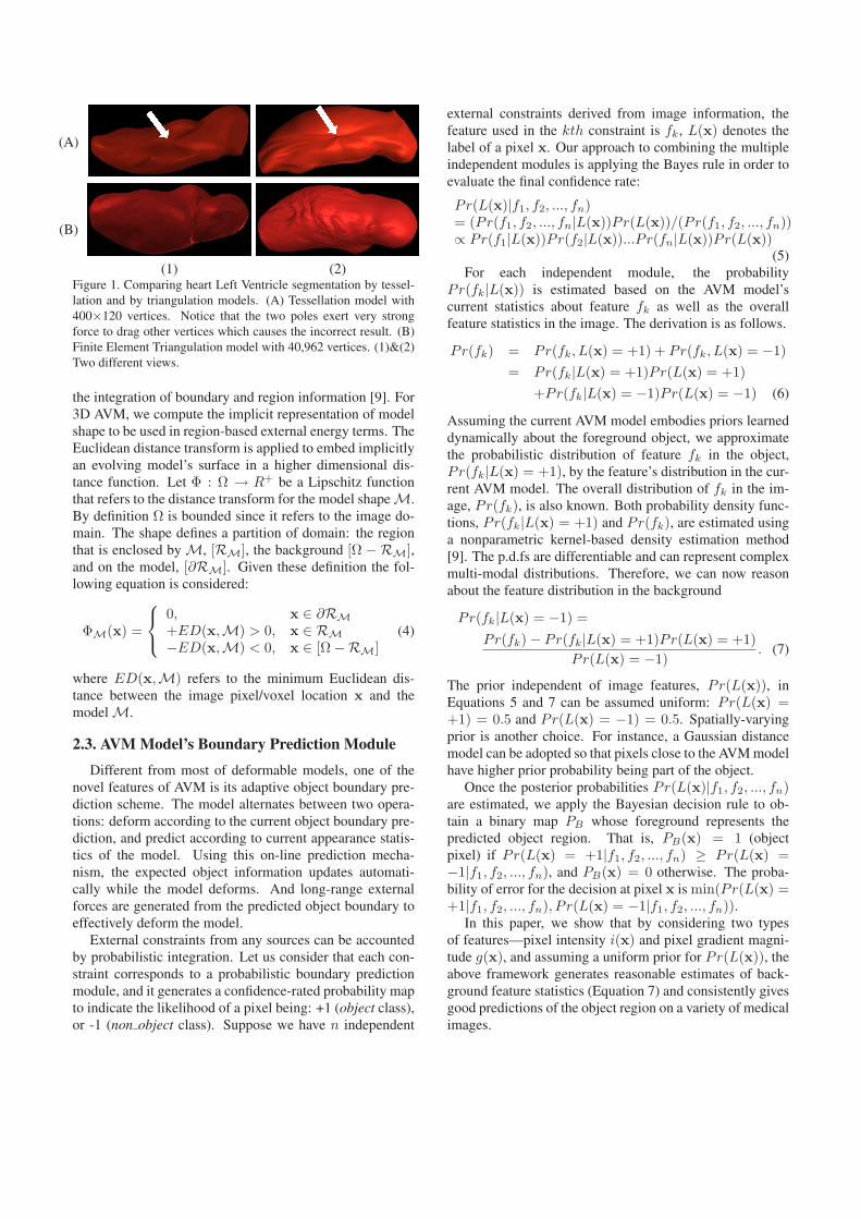
(1) (2) (3) (4)Figure 2. Left Ventricle endocardium segmentation using a 2D ac-tive volume model. (A) The model drawn on the original heartimage. (B) The binary map PB estimated by the boundary pre-diction module. (C) Distance transform of the ROI boundary. (1)Initial model. (2) The model after 8 iterations. (3) The model after18 iterations. (4) Final converged result after 26 iterations.

Given the binary map PB , we apply a connected com-ponent analysis algorithm on PB to retrieve the connectedcomponent that overlaps the current model. This con-nected region is considered as the current Region Of In-terest (ROI) and its boundary represents the predicted ob-ject boundary. Due to noise, there might be small holesthat need to be filled before extracting the boundary of theROI, R. The progressive ROI updating can be clearly seenfrom a 2D AVM example in Figure 2. In the figure, theROI evolves according to the changing object appearancestatistics (estimated by current volumetric model’s statis-tics). And the image forces (Section 3) generated by theROI region energy term deform the model to converge tothe object boundary.

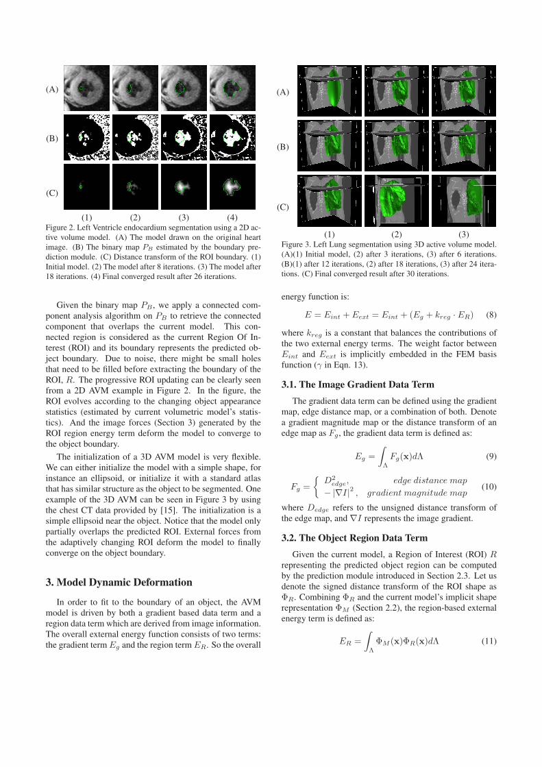
The initialization of a 3D AVM model is very flexible.We can either initialize the model with a simple shape, forinstance an ellipsoid, or initialize it with a standard atlasthat has similar structure as the object to be segmented. Oneexample of the 3D AVM can be seen in Figure 3 by usingthe chest CT data provided by [15]. The initialization is asimple ellipsoid near the object. Notice that the model onlypartially overlaps the predicted ROI. External forces fromthe adaptively changing ROI deform the model to finallyconverge on the object boundary.

3. Model Dynamic Deformation

In order to fit to the boundary of an object, the AVMmodel is driven by both a gradient based data term and aregion data term which are derived from image information.The overall external energy function consists of two terms:the gradient term Eg and the region term ER. So the overall

(A)

(B)

(C)

(1) (2) (3)Figure 3. Left Lung segmentation using 3D active volume model.(A)(1) Initial model, (2) after 3 iterations, (3) after 6 iterations.(B)(1) after 12 iterations, (2) after 18 iterations, (3) after 24 itera-tions. (C) Final converged result after 30 iterations.

energy function is:

E = Eint + Eext = Eint + (Eg + kreg · ER) (8)

where kreg is a constant that balances the contributions ofthe two external energy terms. The weight factor betweenEint and Eext is implicitly embedded in the FEM basisfunction (γ in Eqn. 13).

3.1. The Image Gradient Data Term

The gradient data term can be defined using the gradientmap, edge distance map, or a combination of both. Denotea gradient magnitude map or the distance transform of anedge map as Fg , the gradient data term is defined as:

Eg =∫

Λ

Fg(x)dΛ (9)

Fg ={

D2edge, edge distance map

− |∇I|2 , gradient magnitude map(10)

where Dedge refers to the unsigned distance transform ofthe edge map, and ∇I represents the image gradient.

3.2. The Object Region Data Term

Given the current model, a Region of Interest (ROI) Rrepresenting the predicted object region can be computedby the prediction module introduced in Section 2.3. Let usdenote the signed distance transform of the ROI shape asΦR. Combining ΦR and the current model’s implicit shaperepresentation ΦM (Section 2.2), the region-based externalenergy term is defined as:

ER =∫

Λ

ΦM (x)ΦR(x)dΛ (11)

The multiplicative term provides two-way balloon forcesthat deform the model toward the predicted ROI boundary.This allows flexible model initializations either overlappingthe object or inside the object.

3.3. The Model’s Deformation

Minimization of the 3D AVM energy function can beachieved by solving the following linear system

A3D · V = LV ; (12)

where A3D is the stiffness matrix derived from Equation 3by using the basis function in Equation 13. A3D is symmet-ric and positive definite. V is the vector of vertices on thesurface of AVM. LV is the external force vector correspond-ing to the vertex vector and is obtained from the gradientdata term and region data term. To facilitate the computa-tion, 3D AVM adopts a continuous piecewise linear basisfunction,

φj(vi) = δij ≡{

γ i = j0 i �= j

(13)

where vi is the ith vertex on the finite element triangulationand γ is a positive value to control the smoothness of themodel.

Equation 12 can be solved by using finite differences [3].After initializing the 3D AVM, the final converged resultcan be obtained iteratively based on equation:

(V t − V t−1)/τ + A3D · V t = LV t−1 (14)

where V 0 is the initial AVM vertex vector and τ is the timestep size. Equation 14 can be written in a finite differencesformulation, which yields

M · V t = V t−1 + τLV t−1

M = (I + τA3D) (15)

Using Equation 15, we adopt the following steps todeform the 3D AVM toward matching the desired objectboundary.

1. Initialize the AVM, stiffness matrix A3D, step size τ ,and calculate the gradient magnitude or edge map.

2. Compute ΦM based on the current model; predict R byapplying the Bayesian Decision rule to binarizing theestimated object probability map, and compute ΦR.

3. Deform the model according to Equation 15.

4. Adaptively increase the external force factor in Equa-tion 8, decrease the step size τ in Equation 15 and re-duce γ in Equation 13.

5. Repeat steps 2-4 until convergence.

In Step 4, adaptively changing the weight factors guaran-tees the model can not only reach the desired object bound-ary, but also capture a lot of details on the boundary.

(A)

(B)

(C)

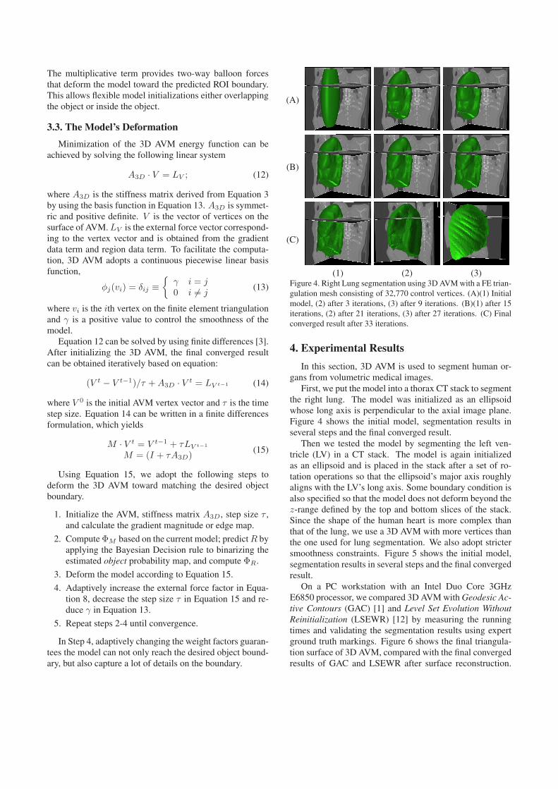
(1) (2) (3)Figure 4. Right Lung segmentation using 3D AVM with a FE trian-gulation mesh consisting of 32,770 control vertices. (A)(1) Initialmodel, (2) after 3 iterations, (3) after 9 iterations. (B)(1) after 15iterations, (2) after 21 iterations, (3) after 27 iterations. (C) Finalconverged result after 33 iterations.

4. Experimental Results

In this section, 3D AVM is used to segment human or-gans from volumetric medical images.

First, we put the model into a thorax CT stack to segmentthe right lung. The model was initialized as an ellipsoidwhose long axis is perpendicular to the axial image plane.Figure 4 shows the initial model, segmentation results inseveral steps and the final converged result.

Then we tested the model by segmenting the left ven-tricle (LV) in a CT stack. The model is again initializedas an ellipsoid and is placed in the stack after a set of ro-tation operations so that the ellipsoid’s major axis roughlyaligns with the LV’s long axis. Some boundary condition isalso specified so that the model does not deform beyond thez-range defined by the top and bottom slices of the stack.Since the shape of the human heart is more complex thanthat of the lung, we use a 3D AVM with more vertices thanthe one used for lung segmentation. We also adopt strictersmoothness constraints. Figure 5 shows the initial model,segmentation results in several steps and the final convergedresult.

On a PC workstation with an Intel Duo Core 3GHzE6850 processor, we compared 3D AVM with Geodesic Ac-tive Contours (GAC) [1] and Level Set Evolution WithoutReinitialization (LSEWR) [12] by measuring the runningtimes and validating the segmentation results using expertground truth markings. Figure 6 shows the final triangula-tion surface of 3D AVM, compared with the final convergedresults of GAC and LSEWR after surface reconstruction.

(A)

(B)

(C)

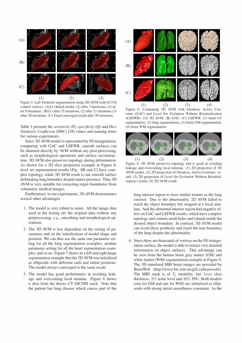
(1) (2) (3)Figure 5. Left Ventricle segmentation using 3D AVM with 65,538control vertices. (A)(1) Initial model, (2) after 3 iterations, (3) af-ter 9 iterations. (B)(1) after 15 iterations, (2) after 21 iterations (3)after 30 iterations. (C) Final converged result after 39 iterations.

Table 1 presents the sensitivity (P), specificity (Q) and DiceSimilarity Coefficient (DSC) [18] values and running timesfor various experiments.

Since 3D AVM model is represented by FE triangulation,comparing with GAC and LSEWR, smooth surfaces canbe obtained directly by AVM without any post-processing,such as morphological operations and surface reconstruc-tion. 3D AVM also preserves topology during deformation.As shown for a 2D slice projection example in Figure 8,level set segmentation results (Fig. 8B and C) have com-plex topology, while 3D AVM result is one smooth surfacedelineating lung boundary despite tumor presence. Thus 3DAVM is very suitable for extracting organ boundaries fromvolumetric medical images.

Furthermore, in our experiments, 3D AVM demonstratesseveral other advantages.

1. The model is very robust to noise. All the image dataused in the testing are the original data without anypreprocessing, e.g., smoothing and morphological op-erations.

2. The 3D AVM is less dependent on the setting of pa-rameters and on the initialization of model shape andposition. We can thus use the same one parameter set-ting for all the lung segmentation examples, anotherparameter setting for all the heart segmentation exam-ples, and so on. Figure 7 shows in a left and right lungssegmentation example that the 3D AVM was initializedas ellipsoids with different radii and initial positions.The model always converged to the same result.

3. The model has good performance in avoiding leak-age and overcoming local minima. Figure 8 showsa slice from the thorax CT DICOM stack. Note thatthe patient has lung disease which causes part of the

(A)

(B)

(C)

(1) (2) (3) (4)Figure 6. Comparing 3D AVM with Geodesic Active Con-tours (GAC) and Level Set Evolution Without Reinitialization(LSEWR). (A) 3D AVM, (B) GAC, (C) LSEWR. (1) heart LVsegmentation, (2) lung segmentation, (3) brain GM segmentation,(4) brain WM segmentation.

(1) (2) (3) (4)Figure 8. 3D AVM preserves topology and is good at avoidingleakage and overcoming local minima. (1) 2D projection of 3DAVM model, (2) 2D projection of Geodesic Active Contours’ re-sult, (3) 2D projection of Level Set Evolution Without Reinitial-ization’s result, (4) 2D AVM result.

lung interior region to have similar texture as the lungexterior. Due to the abnormality, 2D AVM failed toreach the object boundary but stopped at a local min-ima. And the abnormal interior region had negative ef-fect on GAC and LSEWR results, which have complextopology and contain small holes and islands inside thedesired object boundary. In contrast, 3D AVM modelcan avoid these problems and reach the true boundaryof the lung despite the abnormality.

4. Since there are thousands of vertices on the FE triangu-lation surface, the model is able to extract very detailedinformation on object surfaces. This advantage canbe seen from the human brain gray matter (GM) andwhite matter (WM) segmentation example in Figure 9.The 3D simulated MRI brain images are provided byBrainWeb (http://www.bic.mni.mcgill.ca/brainweb/).The MRI stack is of T1 modality, has 1mm slicethickness, 3% noise level and 20% INU. Both models(one for GM and one for WM) are initialized as ellip-soids with strong initial smoothness constraint. As the

Table 1. Quality evaluation and performance comparison3D AVM GAC LSEWR

Organ size (voxels) P Q DSC Time P Q DSC Time P Q DSC TimeLungs (307 × 307 × 187) 93.6 99.8 95.2 1000s 75.7 99.9 85.8 2149s 91.4 99.7 94.6 1840sHeart (256 × 256 × 153) 91.8 99.6 94.3 1044s 78.0 99.8 87.6 1752s 80.1 99.9 88.5 1452sGM (181 × 217 × 180 87.6 98.3 91.5 1620s 75.7 99.0 85.0 2332s 86.4 99.9 89.4 621sWM (181 × 217 × 180) 76.8 96.2 78.3 1833s 66.9 95.5 72.5 2453s 81.1 99.8 89.0 643s

(A)

(B)

(1) (2) (3) (4) (5) (6)Figure 7. 3D AVM has less dependence on model initialization and parameter settings. (A)(1) Initial 3D AVM model, (2) after 3 iterations,(3) after 12 iterations, (4) after 21 iterations, (5) final converged result after 33 iterations, (6) final result viewed from a different viewpoint.(B)(A)(1) A different 3D AVM model initialization on the same image stack, (2) after 3 iterations, (3) after 12 iterations, (4) after 24iterations, (5) final converged result after 36 iterations, (6) final result viewed from a different viewpoint.

models are getting closer to the approximated objectboundary, the models decrease the smoothness con-straint automatically based on the deformation strategydescribed in Section 3.3. Then a lot of details on theobject surfaces appear on the models.

5. Conclusion and Future Work

In this paper, we proposed a novel active volume model,which is a natural extension of parametric deformable mod-els to integrate object appearance and region information.The main contributions include: (1) a clean formulationto integrate online learning and region statistics into ac-tive contours and surfaces, which provides flexible initial-ization and rapid convergence, (2) the finite differencesoptimization framework that enables very fast gradient-and appearance-statistics based model deformations, (3) thecombination of multiple sources of information in a unifiedframework for predicting object region and boundary. Us-ing various experiments on 3D medical images, we demon-strate that the AVM model can perform segmentation effi-ciently and reliably on CT and MRI images. However, dueto the local smoothness of simplex-mesh, it is still hard forthe model to reach details on branch structures (e.g. WM inFigure 9B). In the future, we plan to address this problemby reparameterizing the model near branches since verticesin such areas are sparser than those on the main body.

6. Acknowledgements

The authors would like to thank Prof. Leon Axel(NYU) for providing the heart CT volume data and alsoacknowledge stimulating discussions with Prof. DimitrisMetaxas (Rutgers), Junzhou Huang (Rutgers) and YaoyaoZhu (Lehigh). This work was supported by NSF grant IIS-0812120.

References

[1] V. Caselles, R. Kimmel, and G. Sapiro. Geodesic active con-tours. Internal Journal of Computer Vision, 22, 1997.

[2] T. Chan and L. Vese. Active contours without edges. IEEETrans. on Image Processing, 10:266–277, 2001.

[3] L. Cohen and I. Cohen. Finite-element methods for ac-tive contour models and balloons for 2-D and 3-D images.IEEE Trans. on Pattern Analysis and Machine Intelligence,15:1131–1147, 1993.

[4] T. Cootes, G. Edwards, and C. Taylar. Active appearancemodels. Proc. Of European Conf. on Computer Vision,2:484–498, 1998.

[5] T. Cootes, C. Taylor, D. Cooper, and J. Graham. Active shapemodel - their training and application. Computer Vision andImage Understanding, 61:38–59, 1995.

[6] M. Costa, H. Delingette, S. Novellas, and N. Ayache. Auto-matic segmentation of bladder and prostate using coupled 3Ddeformable models. In MICCAI (1), pages 252–260, 2007.

[7] D. Cremers, M. Rousson, and R. Deriche. A review of statis-tical approaches to level set segmentation: Integrating color,

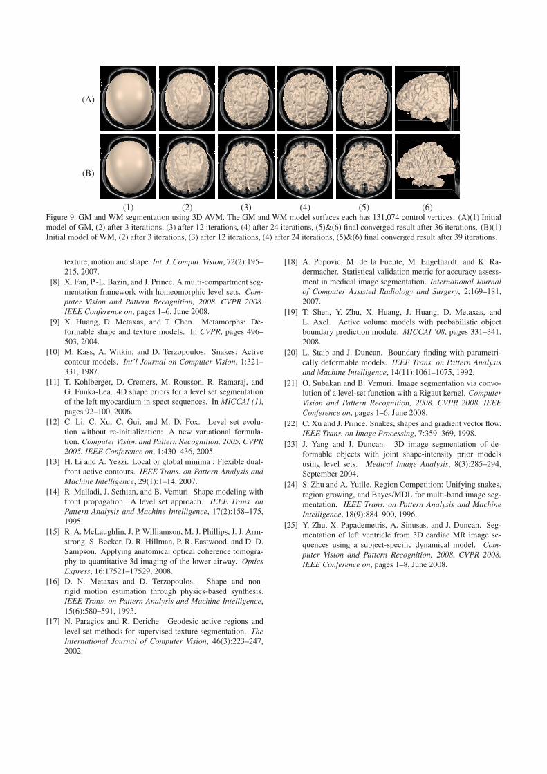
(A)

(B)

(1) (2) (3) (4) (5) (6)Figure 9. GM and WM segmentation using 3D AVM. The GM and WM model surfaces each has 131,074 control vertices. (A)(1) Initialmodel of GM, (2) after 3 iterations, (3) after 12 iterations, (4) after 24 iterations, (5)&(6) final converged result after 36 iterations. (B)(1)Initial model of WM, (2) after 3 iterations, (3) after 12 iterations, (4) after 24 iterations, (5)&(6) final converged result after 39 iterations.

texture, motion and shape. Int. J. Comput. Vision, 72(2):195–215, 2007.

[8] X. Fan, P.-L. Bazin, and J. Prince. A multi-compartment seg-mentation framework with homeomorphic level sets. Com-puter Vision and Pattern Recognition, 2008. CVPR 2008.IEEE Conference on, pages 1–6, June 2008.

[9] X. Huang, D. Metaxas, and T. Chen. Metamorphs: De-formable shape and texture models. In CVPR, pages 496–503, 2004.

[10] M. Kass, A. Witkin, and D. Terzopoulos. Snakes: Activecontour models. Int’l Journal on Computer Vision, 1:321–331, 1987.

[11] T. Kohlberger, D. Cremers, M. Rousson, R. Ramaraj, andG. Funka-Lea. 4D shape priors for a level set segmentationof the left myocardium in spect sequences. In MICCAI (1),pages 92–100, 2006.

[12] C. Li, C. Xu, C. Gui, and M. D. Fox. Level set evolu-tion without re-initialization: A new variational formula-tion. Computer Vision and Pattern Recognition, 2005. CVPR2005. IEEE Conference on, 1:430–436, 2005.

[13] H. Li and A. Yezzi. Local or global minima : Flexible dual-front active contours. IEEE Trans. on Pattern Analysis andMachine Intelligence, 29(1):1–14, 2007.

[14] R. Malladi, J. Sethian, and B. Vemuri. Shape modeling withfront propagation: A level set approach. IEEE Trans. onPattern Analysis and Machine Intelligence, 17(2):158–175,1995.

[15] R. A. McLaughlin, J. P. Williamson, M. J. Phillips, J. J. Arm-strong, S. Becker, D. R. Hillman, P. R. Eastwood, and D. D.Sampson. Applying anatomical optical coherence tomogra-phy to quantitative 3d imaging of the lower airway. OpticsExpress, 16:17521–17529, 2008.

[16] D. N. Metaxas and D. Terzopoulos. Shape and non-rigid motion estimation through physics-based synthesis.IEEE Trans. on Pattern Analysis and Machine Intelligence,15(6):580–591, 1993.

[17] N. Paragios and R. Deriche. Geodesic active regions andlevel set methods for supervised texture segmentation. TheInternational Journal of Computer Vision, 46(3):223–247,2002.

[18] A. Popovic, M. de la Fuente, M. Engelhardt, and K. Ra-dermacher. Statistical validation metric for accuracy assess-ment in medical image segmentation. International Journalof Computer Assisted Radiology and Surgery, 2:169–181,2007.

[19] T. Shen, Y. Zhu, X. Huang, J. Huang, D. Metaxas, andL. Axel. Active volume models with probabilistic objectboundary prediction module. MICCAI ’08, pages 331–341,2008.

[20] L. Staib and J. Duncan. Boundary finding with parametri-cally deformable models. IEEE Trans. on Pattern Analysisand Machine Intelligence, 14(11):1061–1075, 1992.

[21] O. Subakan and B. Vemuri. Image segmentation via convo-lution of a level-set function with a Rigaut kernel. ComputerVision and Pattern Recognition, 2008. CVPR 2008. IEEEConference on, pages 1–6, June 2008.

[22] C. Xu and J. Prince. Snakes, shapes and gradient vector flow.IEEE Trans. on Image Processing, 7:359–369, 1998.

[23] J. Yang and J. Duncan. 3D image segmentation of de-formable objects with joint shape-intensity prior modelsusing level sets. Medical Image Analysis, 8(3):285–294,September 2004.

[24] S. Zhu and A. Yuille. Region Competition: Unifying snakes,region growing, and Bayes/MDL for multi-band image seg-mentation. IEEE Trans. on Pattern Analysis and MachineIntelligence, 18(9):884–900, 1996.

[25] Y. Zhu, X. Papademetris, A. Sinusas, and J. Duncan. Seg-mentation of left ventricle from 3D cardiac MR image se-quences using a subject-specific dynamical model. Com-puter Vision and Pattern Recognition, 2008. CVPR 2008.IEEE Conference on, pages 1–8, June 2008.