ACTIVITY-BASED COSTING FOR

ECONOMIC VALUE ADDED

by

J.S. Jordan, Regina Anctil and Arijit Mukherji

Discussion Paper No. 278, December 1994

Center for Economic Research Department of Economics University of Minnesota Minneapolis, MN 55455

Activity-Based Costing

for

Economic Value Added

by

J.S. Jordan*

Department of Economics and Carlson School of Management,

University of Minnesota.

Regina Anctil**

Haas School of Business,

University of California, Berkeley.

Arijit Mukherji

Carlson School of Management,

University of Minnesota.

December 1994***

* Support from the National Science Foundation is gratefully acknowledged.

** Support from the University of California Regents' Junior Faculty Fellowship is gratefully acknowl­edged.

*** The authors would like to thank workshop participants at Berkeley for their comments.

Abstract

Economic value added (EVA), which is the currently popular term for the traditional

accounting concept of residual income, subtracts from operating income an interest charge

for invested capital. This paper provides both a normative justification for EVA and an

activity-based cost system that supports EVA maximization. We construct a model of

participatory budgeting for a multi-activity firm in which we show that, if investment

decisions are made myopically each period to maximize EVA, the resulting path of plant

and equipment vectors asymptotically approximates the path that maximizes discounted

cash flows. The cost system allocates plant and equipment cost to products using a formula

that includes the interest charge.

1. Introduction

The allocation of fixed cost, especially plant and equipment cost, is one of the most

troublesome problems in all of managerial accounting. If allocated to products, it has

the potential to mislead numerous decisions to which it is economically irrelevant. If it

is not allocated or charged to users in some fashion, management loses an essential tool

for determining the profitability of maintaining or expanding capacity. Two recent trends

in managerial accounting, the widespread adoption of activity-based cost systems and the

increasing popularity of "economic value-added" as a performance measure, have made

the resolution of this traditional dilemma more imperative.

Activity-based costing (ABC) relies on the careful tracing of resource flows within

the firm, but its product cost calculations make no distinction between variable and fixed

resources. Distinctions among resource costs, if any, are made according to the nature of

the demand for resources, rather than the nature of the supply. Thus, ifthe cost driver for

a drill-press is machine hours, for example, then each unit of product will absorb drill-press

depreciation in the same linear fashion that it absorbs material and labor cost. As a result,

the unit cost of a product may overstate the savings that could be realized by producing

fewer units. Firms that replace a simplistic traditional cost system with a more elaborate

and costly ABC system in the hope of identifying and dropping unprofitable products may

make decisions that cause greater reductions in revenue than cost.

Economic value added (EVA), the currently popular name for the traditional ac­

counting concept of residual income, subtracts from operating income an interest charge

for invested capital (Stewart, 1991). When different performance centers share common

plant and equipment, some method must be found to allocate the common capital costs.

More specifically, the cost system needs to allocate plant and equipment costs to products

in a way that embeds the interest charge in the product cost. Otherwise, a performance

center manager will not be able to determine whether any given decision will increase or

decrease EVA.

The present paper constitutes an ambitious two-front attack on the problem of allo-

1

cating plant and equipment cost in a general product cost system. First, we provide a

normative justification for the use of EVA as a performance measure from the viewpoint

of discounted cash flow maximization. Second, we describe an ABC system that includes

specific rules for allocating plant and equipment costs, and show how the resulting costs

support the maximization of EVA.

Before going further, we should clarifY what we mean by "fixed" , or "plant equipment"

cost. Capital goods are distinguished from other inputs by the fact that they are not

consumed by use, but deteriorate over time. A machine that is consumed by use, such as

a printer that has a useful life measured in total pages printed, is conceptually no different

than an inventory of raw materials, and thus does not require a conceptually different

accounting treatment. Inputs that are consumed by the passage of time, independently

of use, require a very different method of cost allocation to avoid distorting the causal

relation between a product and its cost. Such inputs are the focus of this paper. We will

use the term "investment activity" to denote an activity that purchases and installs such

an input, say drill-presses. If the use of the input necessitates maintenance expense, or

the input requires labor to operate, we will suppose that there is another activity that is

responsible for operating the input and incurring those expenses that are caused by its use.

Thus the only expense incurred by an investment activity is the purchase and installation

cost. It is precisely this cost, or its accounting incarnation as depreciation expense, that

is the fixed cost of this paper. In justification of the absence of any distinction between

fixed and variable costs in ABC systems, Cooper (1992, p. B1-10) writes, "Expenses are

not intrinsically either fixed or variable." We take the opposing view that the expenses of

investment activities are intrinsically fixed.

Section 2 gives the formal model of a firm as a collection of productive activities,

extending the model in Jordan (1994) to include investment activities. Section 3 provides

a normative justification for EVA. Since the term residual income (RI) is more common

in the accounting literature, we will refer to RI rather than EVA in the remainder of this

paper. If the firm makes investment decisions each period to maximize RI, the resulting

2

sequence of cash flows will typically fail to ma..ximize present value (PV). However, Anctil

(1993), shows, in a single-good model, that the sequence of investments converges to the

same capital level that is the limit of the PV-maximizing path. Thus residual income

maximization is a myopic period-by-period decision rule that asymptotically approximates

the outcome of the more complex and farsighted present value maximization rule. Section 3

generalizes Anctil's result to the multi-activity setting of the present model. The specific

assumptions needed are discussed at the beginning of Section 3, but one assumption should

be mentioned here. In order for RI maximization to approximate PV maximization, it is

essential that for each capital input, the depreciation rate used in measuring RI is equal

to the rate at which the input deteriorates over time. If the depreciation rate overstates

the "deterioration rate" , for example, then RI overstates the cost of the input, which can

permanently hold investment in the input below the PV-maximizing level.

Section 4 adds investment activity costs to the ABC model constructed by Jordan

(1994). This model is significantly different from others in the small but growing theo­

retical ABC literature, so we should mention its main features. As Noreen (1991) and

Christensen and Demski (1992) have argued, ABC costs are true marginal costs if and

only if the firm has a Leontief, linear fixed-coefficient technology. In this case, as Banker

and Hughes (1994) state, ABC costs provide information that is "economically sufficient"

for the complete description of the production technology. In contrast, we do not assume

linearity, so ABC costs are not an economically sufficient representation of the firm's tech­

nology, and do not equal or reveal the true marginal costs. The imperfection of accounting

information forces the consideration of "second-best" optimality criteria, and also leads us

to ensure that the model is compatible with the use of any additional information that

managers might possess. The ABC costs are used to parameterize performance measures

which activity managers, who know the technology of their own activity but know nothing

about other activities, seek to maximize in a participatory budgeting process. A plan that

maximizes residual income is a budget equilibrium (Proposition 4.15), but there are many

other less desirable budget equilibria as well. However, every budget equilibrium has the

3

"second-best" property that residual income could not be improved by dropping any prod­

uct or out-sourcing any internally produced input (Proposition 4.19 and Remarks 4.20).

Moreover, the activity performance measures are "residual income seeking" in the sense

that if activity managers possess additional information, engage in ad hoc communica­

tion with other managers, or coordinatf' their budget proposals with other managers, their

measured performance will increase if and only if the residual income of the firm increases

(Theorem 4.16). This is the "open architecture" property that allows and encourages the

use of additional information. Section 4.20 contains a specific discussion of the Banker and

Hughes (1994) model and its relation to the present paper.

The asymptotic equivalence of residual income and discounted cash flow maximization

and the result that an RI maximum is a budget. equilibrium rely on the assumption that,

except for fixed costs, the firm's technology is convex. The "second-best" property of

budget equilibria uses the weaker assumption that, except for fixed resources, activities can

be scaled down linearly without violating technological feasibility. Convexity is a pervasive

assumption in managerial accounting theory, but it rules out "step" costs and increasing

returns to scale. In the present paper, speaking very loosely, convexity is limited to long­

run cost and short-run variable cost. Of course. since the calculation of cost is endogenous

to the model, assumptions are stated in terms of technological possibilities.

The specific rule for allocating investment cost is one that we have not seen elsewhere,

so we will devote some discussion to it here. The traditional method of fixed cost allocation

consists of allocating the total cost over some base that corresponds, at least roughly, to

usage of the resource. The cost of a machine, for example, might be allocated over hours

of usage. An unfortunate effect of this procedure is that the budgeted "burden rate", or

cost per hour, depends on the budgeted hours of use. A modification recommended by

Cooper and Kaplan (1992) to remove this effect. is to average the cost over the practical

capacity, and leave the cost of the unused capacity unallocated. While this modification

prevents product managers from being charged for unused resources, it does not go far

enough. In a given period, a capital input is available in a fixed amount at a cost that is

4

not merely fixed but sunk (previously paid or obligated). The maximization of residual

income, or any other economically natural measure of profit, requires that such an input

be utilized up to the point where its marginal contribution is zero, or its practical capacity,

whichever is smaller. The allocation of any of the fixed investment cost could artificially

hold its utilization below capacity. Accordingly, we will calculate a budgeted "burden

rate" based not on the historical cost per unit of practical capacity, but on the unit cost of

budgeted gross investment. If there is no gross investment, which means that the capacity

is being reduced through depreciation, the burden rate is zero, in order to encourage the

full utilization of an economically costless resource.

For example, suppose the investment activity consists of the purchase and installation

of drill-presses, and suppose the firm has chosen a 10% (declining balance) depreciation

rate for this activity. If the capacity available in this period (in hours of machine time)

is k, then the firm estimates that 0.9k will be available next period in the absence

of any purchases and installations this period. In particular, suppose that 10% of the

machines wear out and are scrapped each period. If the usage of machine hours budgeted

for next period, say k', exceeds 0.9k, then some gross investment, say $1, must be

incurred this period. If p is the interest rate at which the firm discounts future cash flows,

then the hourly charge for using a drill-press will be budgeted at (p + 0.1)[1/(k' - 0.9k)]

(plus maintenance, operator labor and other usage related expenses). The second factor,

1/(k' - 0.9k), is the budgeted purchase and installation cost per unit of added capacity.

This is multiplied by 10% because it is depreciated rather than expensed, and also

multiplied by p to add the interest charge used in calculating residual income. If the

usage budgeted for next period is equal to 0.9k or less, then no gross investment is

budgeted and the hourly charge for using a drill-press is budgeted at zero (plus usage

related expenses).

Section 5 discusses the special case of a "stationary state"'. in which the usage of each

capital input is constant over time. and gross investment each period equals depreciation.

In the drill-press example, k = k', so 1/(k' - 0.9k) = 1/0.1k. Since gross investment

5

equals depreciation, I = O.lK, where K is the total book-value of capacity. Hence the

hourly charge for using a drill-press is budgeted at (p + O.l)(K/k), and since budgeted

usage equals k, the budgeted total allocation is (p + 0.1)I<.

Before turning to the formal model, it may be useful to close with two observations on

the scope of the concept of investment activity. First, it will not be assumed that the firm's

technology imposes a fixed ratio between outputs and inputs, which permits considerable

flexibility in defining the units of capital goods. In the drill-press example, a one-year

old drill-press, after depreciation, constitutes 0.9 equivalent units of a new drill-press.

However, with additional maintenence expense, it may produce the same hourly output

as a new machine. In other words, maintenence, or some other input, might serve as a

substitute for the 0.1 equivalent machine units.

Second, fixed resources other than plant and equipment can also be treated as invest­

ment activities. In principle, any resource that, independently of use, is committed for a

length of time exceeding the budget period can be capitalized, and the appropriate interest

and depreciation charges against residual income can be calculated. A natural example is

labor in a firm that has an explicit or implicit long-term committment to its employees.

As a more specific illustration, suppose the firm has a pool of employees engaged in order­

processing. Each employee is paid $25,000 per year in salary, including benefits. When

a new employee is hired, the firm pays $500 to an employment agency and sends the

employee to a software training program that costs the firm $1300 in training expenses,

including the employee's salary during the training program. For simplicity, suppose the

budget period is one-year. If 15% of the order-processing employees leave the firm or

are promoted to other positions each year, then 0.15 is an appropriate depreciation rate

for the employment fee and training expense, making the annual charge against residual

income equal to (p + 0.15) 1,800 in the first year, (p + 0.15) 1, 530 in the second year;

etc. Since the salary is paid contemporaneously with the usage of the resource, the an­

nual interest charge on the capitalized salary expense is simply $25,000. Depreciation,

which in this case is attrition, should not be charged because it reduces the salary liability

6

by the same amount that it reduces the capitalized value. Instead, the "book-value" of

the salary committment can be recalculated each period by counting the employees who

remain. Gross investment corresponds to hiring new employees. Suppose the firm hires

one new employee, who is expected to provide 2,000 hours of order-processing capacity.

Then, by the same method as in the earlier drill-press example, one obtains a budgeted

hourly charge for order-processing equal to [25,000 + (p + 0.15)1, 800J/2, 000.

7

2. The Firm This Section models the firm as a collection of productive activities. As in

Jordan, (1994), the model includes cost activities, which incur cash outflows in order to

produce inputs for other activities, and revenue activities, which use the goods or services

produced by the cost activities in order to produce cash inflows. 1]1 addition, the present

model includes a special class of cost act.ivities, termed investment activities, which incur

cash outflows in order to provide capital goods such as those that typically appear in plant

and equipment accounts. Since the basic activity model is described and illustrated by

examples in Jordan (1994), most of the expository comments in the present paper will be

limited to investment activities.

2.1 Plans: There are n activities. The first m activities are cost activities, of which the

first .e are investment activities. The remaining n - m activities are revenue activities. An

action for an activity is a vector Yi E Rm.+l, with coordinates (YiO, ... , Yim). The first

component, YiO, denotes a cash flow. If i # j, -Yij denotes the amount of the output

of activity j that activity i uses as an input. For a cost activity i, Yii denotes the

amount of output. Each activity i has a p1'Oposed action set pi C Rm+l. The proposed

action sets for the different types of activities are as follows:

i) for i = 1, ... ,.e. pi = {Yi E Rm+l : YiO S; 0, Yii 2: O.

and Yij = 0 for all j other than 0 and i};

ii) for i = .e + 1, , ... ,m, pi = {Yi E Rm +1 : YiO S; 0, Yii 2: 0,

YiO < 0 if Yii > O. and Yi) S; 0 for all j # i}; and

iii) for i = m + 1, ... , n, pi = {'/)., E Rm.+l : 1)'0 > 0 • I • l _ , y" < 0 . lJ _

for all j 2: 1, and Yij < 0 for some j 2: 1 if YiO > O}.

Let P = IIi=l pi. A plan is an n-tuple of proposed actions (Yi)i E P. A sequence of

plansis a sequence {(YD J ~ 1 C P.

8

2.2 Feasible Plans:

Each activity i = e + 1, ... , n has a feasible action set yi C pi. Each investment

activity i = 1, ... , e has an investment outlay function Ii : R! ---+ R+. Each investment

activity 't has a feasible action cor-respondence yi: R+ ---+---+ pi defined by:

A firm f consists of investment outlay functions (Ii):=1 and feasible actions sets

(yi)~=H1' A plan (Yi)~=1 E P is feasible for f given kO E R~ if

i) for each i = 1, ... ,e, 1/· E yi(kO). '. t 'l ,

ii) for each i = I! + 1, ... , n, Yi E yl; and n

iii) for each j = 1, ... ,m" LYij 2: O. i=1

A sequence of plans {(yDJ:1 is feasible for f given kO if for each t, (YDi is feasible

for f given kt-1, where

iv) k t- 1 _ {k(~Ot_l i-I) Yu , ... , Ya.

if

if

t = 1;

t > 1.

and

2.3 Remarks: Capital goods are distinguished from other inputs to by the fact that they

are consumed through depreciation rather than use. For this reason, we will refer to the

output of an investment activity as capacity. For example, the capacity provided by a

building might be measured as floor space, while the capacity of a Xerox machine might

be measured in pages per month.

Since capacity is reduced by depreciation rather than use, the cash outlay needed by

investment activity i to provide yri 1 units of capacity in period t + 1 depends on the

amount of capacity that was provided in period t. For example, the investment outlay

function might take the form

9

where hi > 0 represents the unit cost of pmchasing and installing capacity, and diY!i

measures the amount of capacity lost through depreciation, so that Y~tl - (1 - di)Y!i is

the amount of capacity that must be pm chased and installed in order to provide Yftl,

assuming that y:t1 2: (1 - di)Y!i'

If Yi is a proposed action by activity i, then for any cost activity j =1= i, -Yij is

the amount of the output of activity j that activity i proposes to use as input. We

will often refer to the output of cost activity j as "commodity j". The sum 2:7=1 Yij is

the net supply of commodity j, so the feasibility condition 2.2(iii) states that the total

usage of commodity j cannot exceed the amount produced. For an investment activity

i, every proposed action Yi E pi has Yij = 0 for every cost activity j =1= i. The need for

this restriction is explained in 2.8 below.

The cash flow, YiO, generated by a revenue activity i is not explicitly represented

as revenue from the sale of a good or service. \Vhile the revenue, YiO, and the cost of

the inputs, -Yil, ... , -Yim, used to produce the revenue are economically relevant, the

decomposition of revenue into price and quantity of sales is irrelevant. However, in order

to obtain a unit cost of the commodity sold by revenue activity i, the quantity of sales

must be represented somewhere. For this purpose, one can model the production of the

commodity as a cost activity j, so that -Yij is the quantity of sales.

The firm must specify a discount rate p > 0 in order to evaluate the present value of

a sequence of plans. Since residual income involves a charge for depreciation, the firm must

specify a depreciation policy for each capital good i. \Ve will assume that the declining

balance method is used, with a depreciation rate 8i > O. It should be emphasised that

except for explicit assumptions stated below. fJ i is an accounting depreciation rate applied

to the book-value, J{i, of the capacity ki , and need not bear any relation to the physical

deterioration of capacity reflected by the investment outlay function Ii. In addition, there

is an initial book-value, K?, which may reflect historical pmchase and installation costs.

The following definitions formalize these specifications.

10

2.4 Capital Policy Parameters: The capital policy parameters for a firm consist of a

discount rate p > 0, a depreciation mte Di 2: ° for each i = 1, ... ,f, and an initial

book-value vector KO E ~~.

2.5 Present Value: Given a discount rate p > 0, the present val'ue of a sequence of

plans {(yDi}:l is:

A sequence of plans is present value maximizing for a firm f gwen kO E ~~ if it is

feasible for f given kO and if there is no other sequence of plans that is feasible for f

given kO and has a higher present value.

2.6 Remarks: The definition of present value indicates our timing convention that the

investment outlay occurs in the period before the capacity is available for use. Thus, if

yf E Yi (k~-l) then the cash outlay - Y!o occurs in period t - 1, and the capacity supply

yfi occurs in period t. Of course, if the committed cash outlays span several periods,

then -yfo represents the period t - 1 discounted value of the cash outlay stream. For

all activities i 2: f, the cash and commodity flows specified by a proposed action yf all

occur in period t. This timing convention is also reflected in the following definition of

residual income.

2. '7 Residual Income: Given a discount rate p > 0, a depreciation rate Di for each

i = 1, ... , e, and initial book-value vector KO E ~~, the residual income of a plan is

defined as 11 e I.: YiO - I.:(p + Di)Ki

i=l+li=l

where

Ki = (1 - D;)Kf - YiO for each i = 1, ... ,e.

11

A plan (Yi)i is residual income maximizing /01' a firm f gwen kO E R~ if it is feasible

for f given kO and there is no other plan that is feasible for f given kO and has a

higher residual income. A sequence of plans {(yDJ:l is 1'esidual income maximizing for

f given kO if it is feasible for f given kO and for each t = 1, ... , the plan (YD i is

residual income maximizing for f given k t - 1 , as defined in 2.2(iv), and given the initial

book-value vector K t - 1, where, for each t 2 0 and each i = 1, ... , f,

if

if

t = 0;

t 2 1.

and

2.8 Remarks: It is not possible to define the present value of a plan (yDi without

reference to future plans (yJ+S)i' s = 1, .... In contrast, the residual income of a plan

(yDi requires no forecast of future actions, and no knowledge of future business conditions.

However, the myopic nature ofresidual income depends on our assumption that investment

activities do not use the outputs of any other cost activities. For example, a natural

violation of our assumption would be a construction firm that constructs its own warehouse.

In this case, a decision in period t to construct additional warehouse space for period

t + 1 must be anticipated in period t - 1 in order to provide the equipment needed

in period t. The same problem can arise indirectly if an investment activity uses a cost

activity that uses an investment activity. Our definition of the investment outlay function

Ii implicitly assumes that the capacity to be made available in period t can be decided in

period t - 1. This assumption can be interpreted as an implicit definition of the minimal

budget period for which residual-income is defined. Such an assumption is needed because

residual income maximization is obviously inconsistent with any expenditure that produces

no benefits until after the residual income horizon.

2.9 Other Fixed Costs: Many costs that are typically viewed as fixed are not associ­

ated with committed resources. If lights can be turned off in unused areas of a factory,

for example, then factory lighting is not a committed resource, even though it does not

12

vary directly with production volume. In this case, factory lighting can be treated as a

noninvestment cost activity that, along with the investment activity, "available factory

floor space" , serves as an input to the noninvestment cost activity, "useable factory floor

space". Thus, the inclusion of investment activities in the model of the firm also makes

possible the inclusion of a broad spectrum of noncapital fixed costs that are incurred along

with capital investments in the provision of useable capacity.

3. The asymptotic equivalence of residual income and present value maximiza­

tion

This section provides the normative justification for residual income maximization

(for brevity, the acronym PVM (resp. RIM) will be used for both the noun, present

value maximization (resp. residual income maximization) and the adjective, present value

maximizing (resp. residual income maximizing)). PVM requires infinite foresight, while

RIM looks but one period ahead. As a result, the two objectives typically produce different

investment decisions in every period. Nonetheless, under the assumptions described below,

RIM and PVM paths approach identical long-run limits. This result, which is the main

objective of this section, justifies the interpretation of RIM as a practical approximation

to the PVM ideal.

Residual income involves a charge for accounting depreciation, so we will need to

assume that accounting depreciation is an accurate measure of the physical deterioration

oLcapacity. More precisely, we will assume that for each investment activity i, if kf is

the available capacity in period t, then (1 - l5i ) kf will be costlessly available in period

t + 1. To simplify the analysis, we will ignore the possibility of scrapping capacity and

limit disinvestment to depreciation by imposing, as a feasibility condition, that kt+ 1 2:

(1 - l5i )kf. We will also assume that the purchase and installation of additional capacity,

above (1 -l5i )k;, requires an outlay of hi dollars per unit. The unit cost, hi, which

will be assumed positive, affects the desired capacity, but does not prevent the firm from

13

moving to the desired capacity at once, in which case the main result of this Section holds

trivially. In order to make the result nontrivial, we will include in the investment outlay a

cost of expansion, ei(kf+l - kD, so that the investment outlay function takes the form

J.(kt kt+l) = h· [e+ 1 - (1 - b·)kt] + e(kt+l - e) t t' t t '., t t t t 'l •

The expansion cost function, which was introduced in an optimizing model of business

investment by Eisner and Strotz (1963) (see also Sargent (1979, Chapter VI)), represents

the premium paid to increase capacity by the amount kf+l - kf in a single period, rather

than spreading the increase over the indefinite future. For example, let ei (kf+l - kD =

a·(e+1 - kt)2 for kt+1 > kt where az' is a positive constant. Since we have limited t 'l t t - t'

disinvestment to depreciation, we will assume that ei(k;+l - kD = 0 if kf+l ~ k;,

so that there is no premium for adjusting capacity downward. This specification of the

investment outlay function is stated formally as Assumption I (3.2), and the requirement

that kf+l ~ (1 - bi)kf is imposed in the definitions of RIM (3.10) and PVM (3.16).

Anctil (1994) proves the asymptotic equivalence of PVM and RIM in a two-activity

model with a single capital good. Anctil also assumes that net revenue is a strictly concave

differentiable function of the single capacity level, and that the expansion cost function is

differentiable and strictly convex. Anctil's proof of asymptotic equivalence exploits the one­

dimensional nature of the investment dynamics in her model. In the present multi-activity

model, the number of capital goods is arbitrary, and the net revenue obtainable from any

vector of capacities is not a primitive of the model, but must be derived as the solution of

a constrained ma..'(imization problem involving the feasible sets yi, i = l + 1, ... ,n. Thus

the proof given below is necessarily quite difIerent from Anctil's. The result proved here

is much more general, but is weaker in one important respect. Anctil proves that an RIM

path converges to the long-run steady-state at an exponential rate, assuming that the net

revenue function has a strictly negative second derivative. The more abstract setting of

the present model does not seem conducive to rate of convergence results. This issue is

discussed in more detail at the end of t his section.

14

The proof of asymptotic equivalence is quite lengthy, so it may be useful to begin

with an informal overview. Both PVM and RIM require, within each period, that cost

and revenue activity vectors be chosen to ma.ximize short-run net revenue subject to the

current capacity vector. Accordingly, the first order of business is to obtain a well-behaved

net revenue function, r, that gives the maximum short-run cash flow, r(kt), obtainable

from any capacity vector kt. This is accomplished by Proposition 3.5 and Lemma 3.6.

The assumptions used to prove that r is well-defined and continuous (Assump­

tions 3.2) suffice to carry us almost to the final result. We assume that each activity set

yi is closed (Assumption C), that each yi satisfies the down-scaling assumption of Jor­

dan (1994) (Assumption D), and that no cost activity can produce positive output without

some cash expenditure (Assumption N). The down-scaling assumption, which states that

any activity vector that is technologically feasible remains feasible if it is reduced in scale, is

included here largely because of its pervasive role in later sections of this paper. However,

by including it here, we are able to weaken the boundedness assumption needed to ensure

the existence of a short-run profit maximum. In particular, we assume only that for each

revenue activity, average revenue approaches zero at infinite scale (Assumption B). We also

include in Assumption C the assumption that each expansion cost function is continuous,

which is needed to prove the existence of presf'nt value and residual income maxima.

The next stage of the proof consists of parallel but separate analyses of RIM and

PVM paths. Taking RIM first, we show that there is a well-behaved function Vr with

th.e Lyapunov property that along an RIM path, vr(kt) is monotonically increasing.

The function Vr plays the role of a Lyapunov function in the proof that kt ~ Sr, where

Sr denotes the set of capacity vectors that are steady-states (remain stationary) under

RIM (Proposition 3.15). (Like many conwrgence proofs in economic theory, our proof

roughly follows Lyapunov's Second Method (e.g .. Lefschetz (1977) and Lucas and Stokey

(1989), from which the term Lyapunov junctiun originates.) The analysis of PVM paths

is more intricate because the object of choice is the entire infinite sequence of capacity

15

vectors. Nonetheless, there is a function vp that serves as a Lyapunov function proving

that kt --+ Sp, where Sp is the set of steady-states under PVM (Proposition 3.30).

The final stage consists of the proof that Sr = Sp. It is shown that pvp(·);:::: vr(·)

(Proposition 3.31) and that equality holds on Sp, which helps to prove that Mr C Sp C Sr

(Propositions 3.32 and 3.35), where NIr denotes the set of capacity vectors that maximize

Vr. The final step, showing that Sr C Mr (Proposition 3.37), requires us to assume that

the sets yi are convex and that the marginal expansion cost is zero at zero (Dej(O) = 0).

The need for these two additional assumptions is discussed following Proposition 3.35.

Theorem 3.39 is the formal statement of asymptotic equivalence.

The mathematical tools used below are conventional in the economic theory of opti-

mization (e.g., Debreu (1959, Chapter 1) or Border (1985, Chapters 11 and 12». As in

Debreu (1959), the maximum norm is the most convenient for calculations.

3.1 Definitions: On any Euclidean space RP. the norm II· II : RP --+ R+ that will be

used throughout this paper is the maxim'um nO'/'m, II:rll = max Il:jl. For each x E RP and J

each nonempty set S C RP, define d(;r, S) = illf{llx - yll : YES}.

3.2 Assumptions: The following assumptions are imposed throughout this section.

B (Boundedness): For each revenue activity i = m + 1, ... ,n, and each sequence

{yn::l c yi, if IIYi II --+ 00 then lim sup yfo / IIYi II = o. S--I'X)

C (Continuity): For each activity i = f+ 1. ... ,n, yi is closed, and for each investment

activity i = 1. ... , f, Ii is continuous.

D (Down-scaling): For each activity i = J! + 1, ... , n, Ayi E yi for every yi E yi and

every 0:::; A :::; 1.

N (No free production): For each cost activity i = £ + 1, ... ,m, if Yi E yi and

Yii > 0 then YiO < O. For each revenue activity i = m + 1, ... ,n, if Yi E yi and

YiO > 0, then Yij < 0 for some j = 1 .... ,m.

16

I (Investment outlay specification): For each investment activity i = 1, ... ,.e, bi > 0

and there is a number hi > 0 and an expansion cost function ei : R --+ R+ such that

ei(x) = 0 for all x:::; 0, and for each (ki' kD E R~,

where [.j+ denotes max{[·], O}.

The following lemma establishes the boundedness needed to ensure that solutions exist

to the residual income and present value maximization problems.

3.3 Boundedness Lemma: Let {kS}~l C?R~ and let {(Yn~=f+d:l C IIi=f+l pi

satisfy, for each s,

i)

ii)

iii)

yt E yi for each 'l;

n

e + " yS, > 0 for each J' = 1, ... , I!.; and J ~ tJ-

i=i+l n

2: ytj ~ 0 for each j = .e + 1, ... , m. i=i+l

For each s, let ZS = L:l+l Yfo. If for some cost activity iO, yfoio / max{l, Ilksli} --+ 00,

then ZS --+ -00.

Proof: Suppose that for some iO, Y:'jio) / max{l, IlkSII} --+ 00. The feasibility condition

(ii) implies that, taking a subsequence if necessary, we can choose iO so that, ytoio ~ Iytj I

for all i >.e and all j ~ 1. Reunumbering activities if necessary, suppose that iO = m.

By Assumption B, yfo / y':nm --+ 0 for each i > m. Therefore lim sup ZS / y:nm =

limsup(L::l+l yro) / y~~m :::; limsup.IJ;~~o / !l;~'lll' If 1imsupy~~o / Y:nm < 0, then since

y:nm --+ 00, ZS --+ -00. Suppose by way of contradiction that limsupy:no / y:nm = o.

17

For each s, let y':n = (l/y:nrn)Y:n' By Assumption D, Y'~l E ym for each s. Taking a

subseq uence if necessary, y':n ~ y:n for some y:n E ?Rrn+ 1. By Assumption C, y:n E ym.

However, by the definition of y':n, y:nm = 1 and y:no = 0, which contradicts Assumption

N .•

3.4 Definition: Let r:?R~ ~?R be defined as r(k) = max{I::~=l+l YiO:

i)

ii)

iii)

Yi E yi for each '/.; n

kj + L Yij ~ 0 for each j = 1, ... , f; and i=£+l

n

L Yij ~ 0 for each j = f + 1, ... , m}. i=l+l

3.5 Proposition: Under Assumptions 3.2, T is a well-defined continuous function.

Proof: Let a > 0 and let J(a = {k E ?R~ : Ilkll ::; a}. We will show that r is

well-defined and continuous on J(a. Let Y = ITi=l+l yi, and define the correspondence

I : J(a ~~ y by I(k) = {y E Y:

i)

iii)

n

kj + L Yij 2:: 0 for each j = 1, .... f; i=f+l

11

L Yij ~ 0 for each j = e + 1, ... , m; and i=f+l

n

L YiO ~ a}. i=l+l

By Assumption D, with A = 0, 0 E yi for f'(tch i. so f(k) =1= 0 for all k. Therefore

r(k) = max{I::~=e+l YiO : Y E f(k)} for each k E J(a. By Assumption C, I has a

closed graph. Because of the constraint (iii) in the definition of I, Assumption B and the

18

Boundedness Lemma imply that there is a compact subset ye c Y such that the graph

of I is contained in J(a x ye. Therefore f is upper semi-continuous (Debreu (1959,

p. 17)). In particular, for each k Ega, f(k) is compact, so 1'(k) is well-defined. It

remains to show that f is lower semi-continuous (Debreu (1959, p. 17)). Let {k S }:'l

be a sequence in J(a converging to some k, and let y E f(k). For each s, define

AS = max{A : A $ 1 and AY E l(kS)}, and let yS = ASy. By Assumption D, AS is

well-defined for each s. For each s, AY E f(kS) if and only if AY satisfies (i) above

for kS. Since kS ~ k, AS ~ 1, so yS ~ y. Thus I is lower semi-continuous; therefore

r is continuous on J(a by the Berge Maximum Theorem (Debreu (1959)). Since a is

arbitrary, the result follows. •

3.6 Lemma: For any sequence {kS}:'l C ~~ with Ilksll ~ 00, r(kS) / Ilksll ~ O.

Proof: Assumption D with A = 0 implies that r(k) ~ 0 for all k E ~~. If

limsupr(kS) < 00 the result is immediate, so suppose that, taking a subsequence if

necessary, r(kS) ~ 00. For each s, let (yi)7=f+l achieve the maximum that defines

r(kS). Assumption B, together with the feasibility constraint (iii) in the definition of

r(kS) (Definition 3.4), implies that for some cost activity i, r(k S) / yti ~ O. The

Boundedness Lemma implies that lim sup yti / II kS II < 00, so r (kS) / II kS II ~ o. •

We now turn to the analysis of RIM. Residual income is simply net revenue minus a

charge for capital. The capital charge is based on the book-value of capital, which involves

past prices of capital goods. The Lyapunov function V7' mentioned above is obtained

by valuing previously acquired capital at tIlt" current prices hj rather than past prices.

The valuation of previously acquired capital at current prices is necessary to ensure that

the ma..ximized value of residual income is increasing along an Rn/! path. Otherwise, since

initial book values are arbitrary, the depreciation of previously acquired capital can have

an arbitrary effect on residual income. Proposition 3.8 shows that, since the revaluation

pertains only to previously acquired capital. it does not affect the RIM capacity vectors.

1!J

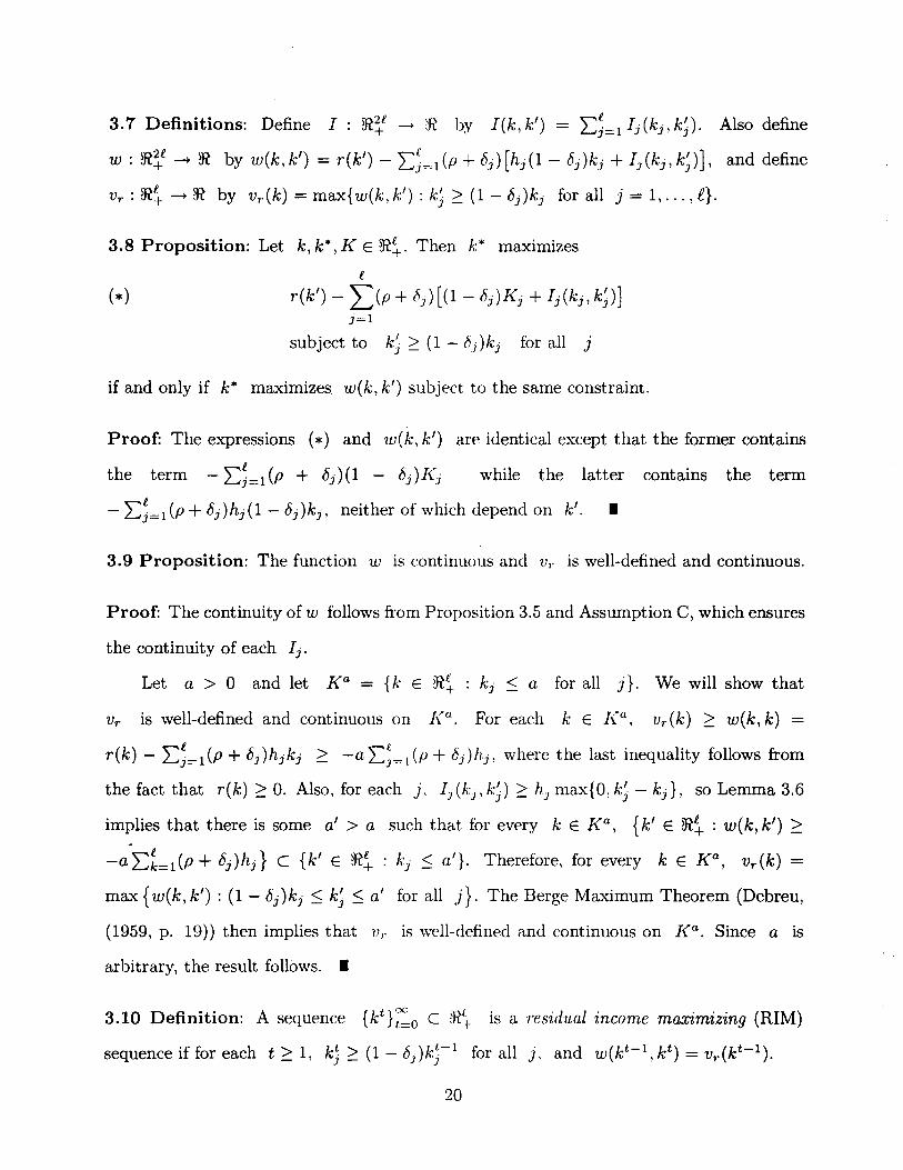
3.7 Definitions: Define I: ~~i ~ R by I(k,k') = L~=IIj(kj,kj). Also define

w : R!i ~ R by w(k, k') = r(k') - L~=1 (p + bj) [hj (1 - bj)kj + Ij(kj , kj)], and define

Vr : R~ ~ ~ by v7·(k) = max{w(k, k') : kj ~ (1 - bj)kj for all j = 1, ... , fl.

3.8 Proposition: Let k, k*, K E R~. Then k* maximizes

l

r(k') - I)p + 8j ) [(1 - bj)Kj + Ij(kj , kj)] j=1

subject to kj ~ (1 - Il j )kj for all j

if and only if k* maximizes w(k, k') subject to the same constraint.

Proof: The expressions (*) and w( k, k') are identical except that the former contains

the term - L~=l (p + bj)(1 - bj )Kj while the latter contains the term

- L~=l (p + bj)hj (1 - bj)kj , neither of which depend on k'. •

3.9 Proposition: The function w is continuous and VI' is well-defined and continuous.

Proof: The continuity of w follows from Proposition 3.5 and Assumption C, which ensures

the continuity of each I j .

Let a > 0 and let Ka = {k E ~~ : kj :::; a for all j}. We will show that

Vr is well-defined and continuous on KD. For each k E Ka, ur(k) ~ w(k, k) =

r(k) - L~=l(P + bj)hjkj ~ -aL~=I(p + I5j )hj , where the last inequality follows from

the fact that r(k) ~ O. Also, for each j, Ij(kj,kj) ~ hj max{O,kj - kj }, so Lemma 3.6

implies that there is some a' > a such that for every k E Ka, {k' E ~~ : w(k, k') ~

-a L~=l (p + bj)hj } C {k' E ~~ : kj :::; a'}. Therefore, for every k E Ka, vr(k) =

max {w(k,k') : (1- bj)kj :::; kj :::; a' for all j}. The Berge Maximum Theorem (Debreu,

(1959, p. 19)) then implies that v,. is well-defined and continuous on Ka. Since a is

arbitrary, the result follows. •

3.10 Definition: A sequence {kt}:o C !R~ is a 'residual income maximizing (RIM)

sequence if for each t ~ 1, kj ~ (1 - I5 j )kr 1 for all j, and w(kt- 1 , kt) = vr(kt- 1 ).

20

3.11 Lemma: For every k E ~~ and every k' E ~~ satisfying kj ~ (1 - 6j )kj for

each j, w(k,k'):S; r(k') - L.~=1(p+6j)hjkj = w(k',k').

Proof: For each j, ej(kj-kj)~O, so Ij(kj,kj)~hjmax{O,kj-kj}. The result now

follows from the definition of w. •

The following proposition establishes the Lyapunov property of vr .

3.12 Proposition: If {kt}~o is an RIM sequence then for each t, Vr(kt+l) ~ vr(kt).

inequality follows from the definition of Vr , the second from Lemma 3.11, and the final

equality from the definition of an RIM sequence. •

3.13 Lemma: For every real number a. the set {k E ~~ : v1·(k) ~ a} is compact.

Proof: That the set is closed follows from tlw continuity of Vr (Proposition 3.9). Lem­

mas 3.11 and 3.6 imply that the set is bounded. •

3.14 Definitions: Let Sr = {k E ~~ : vr(k) = w(k, k)}.

3.15 Proposition: If {kt}~o is an RHvl sequence then d(kt, Sr) - O.

Proof: By Lemma 3.13 and Proposition 3.12, the sequence {kt}~o is bounded. Therefore

it suffices to show that if k* is a cluster point of the sequence then k* E Sr. Choosing

a subsequence {kS}:o' if necessary, we can assume that kS - k*. By Lemma 3.11, for

each s,

By the continuity of Vr and w (Proposition 3.9), w(k S, kS

) - w(k*, k*) and vr(kS)_

vr(k*). By Lemma 3.13, there is some real number v* such that vr(ks- 1) - v* and

vr(kS) - v*. Hence by (1), v* = w(k*, k*) =vr(k*), which proves that k* E Sr. •

21

Proposition 3.15 states that all RHvl paths converge to the set of RIM-stationary

capacity vectors, which completes our analysis of RIM dynamics. We now turn to the

parallel, but unfortunately somewhat more intricate analysis of PVM dynamics. We first

define the Lyapunov function vp mentioned above by subtracting the value of previously

acquired capital, at current prices, from the net present value of current and future cash

flows. As in the case of residual income maximization, this transformation eliminates the

valuation effect of a large initial endowment which is not profitable to maintain.

PVM requires choosing the entire sequence of capital vectors at once, which makes

the existence and good behavior of maxima dependent on ruling out unbounded sequences.

We will take the approach of imposing an artificial upper bound, a, on the size of the

capital vector that can be chosen for any period, and showing that the bound can be made

large enough to make the set of artificially constrained PVM paths identical to the set

of true PVM paths.

3.16 Definitions: For each kO E 1R~, define vp(kO) = max { 2::'1 (1 + p)-t [r(kt) -

I(kt kt+1)] - l(kO k 1) - ~e h -(1 - 8 -)kO . kt+1 > (1 - 8 -)k~ for each t > 1 and each , , L.....J=1 J J 'J' 'J - J J -

j}. For each a> 0, define Ka = {k E 1R~ : kj ~ a for all j}, and for each kO E Ka,

define v;(kO) by imposing the additional constraint that kt E Ka for all t 2: 1 on the

maximum that defines vp(kO). A sequence {k'}:o c 1R~ is a present value maximizing

(PVM) sequence if the sequence {kt } ~ 1 solves the constrained maximization problem

that defines vp(kO). Given a > 0, if IIkoll ~ a and {kt}:l solves the constrained

maximization problem that defines v~ (kO) , then {kt } :0 is called a P VlvF sequence.

3.17 Proposition: For each kO E 1R~, a sequence {k*t}:1 maximizes

00

I: (1 + p)-t [r(kt) - [(e. /;;1+1)] - l(kO, /;;1)

t=1

subjectto k~2:(1-8j)/;;tl foraH t2:1 andall J

if and only if the sequence achieves the constrained maximum that defines vp(kO). More-

22

over, if a> 0 and IIkll ~ a, then {k*t}:l maximizes (*) subject to kj ~ (1-h j )k}-1

for all t ~ 1 and all j and the additional constraint that kt E f{a for all t ~ 1 if and

only if the sequence achieves the constrained maximum that defines v;(kO).

Proof: The maxim and in the definitions of vp(kO) and v;(kO) differs from (*) only by

including the term - E~=1 hj (1 - hj)kJ, which is independent of kt for all t ~ 1. •

3.18 Lemma: For each a > 0 and each PVMa sequence {kt}:o, the sequence

{kt+S}:o is also a PVMa sequence for every positive integer s.

Proof: This follows directly from Proposition 3.17. •

3.19 Proposition: For each a > 0, the function v; f{a ----; R is well-defined and

continuous.

Proof: By Proposition 3.5, r is continuous, and Assumption C ensures that each I j is

continuous. Therefore the function (k, k') t---;. r(k) - I(k, k') is a continuous function on

the compact set f{a x f{a. The result now follows from the fact that (1 + p) > 1 and

the Berge Maximum Theorem (Debreu (1959, p. 19)). •

3.20 Lemma: For each a > O. let Ta =r(a, ... , a). Then for each a > 0 and each

k E f{a, f

v;(k) ~ Ta / p - L h.i(1- hj)kj . j=1

P~oof: Since r is nondecreasing, r( k) ~ ra for all k E f{a. The result now follows

directly from the definition of v;(k). •

We want to establish the Lyapunov property of v;. In order to do this we define a

function v;_ and show that its value at k t+1 always falls between v;(kt) and V;(kt+l)

along the PVM path. The function v;_ is the same as v~ except that it restricts the firm

to remain at its initial capacity level for one period rather than moving to k1 on the PVM

23

path. The effect of this restriction is that each step along that path occurs one period

later. The proof of the Lyapunov property follows from the fact that if the firm were to

have kl on the PVM path initially, then staying at kl an extra period is better (weakly)

than going from kO to kl, but not as profitable as being allowed to move to the PVM k 2 •

3.21 Definition: For each a > 0 and each k E Ka, define v;_ (k) = 2::1 (1 + p)-t

[r(kt-l)-J(kt-l,kt)]-2:~=lhjkj, for any PVMa sequence {kt}:'o with kO=k.

3.22 Lemma: Let a> 0 and let {k'}:'o be a PVMa sequence. Then for each t

Proof: By Lemma 3.18, it suffices to prove the result for t = O. Since 2:~=1 hjk; ~

2:~=1 hj (1 - 8j )kJ + J(kO, kl), it follows from the definitions of v; and v;_ that

v;(kO) ~ v;_ (k1). By Lemma 3.18. the sequence {k t+1 }:'l achieves the constrained

ma..ximum that defines V;(kl). However, v~_ (kl) is obtained by evaluating the maximand

in the definition of v;(kl) at the sequence {kt}:'l' so v;_(kl) ~ V;(kl). •

3.23 Lemma: Let aD > O. Then there is some a* > aD such that for every k E Kao,

v;(k) ~ v;· (k) for every a > a*.

Proof: If not, there is an increasing sequence {as}: 1 with a 1 > aD and as -

00, and a sequence {kS}:'l C Kao with the property that v;s(kS) > v;·-l(kS) for

each s. It follows from the definition of v;~ that for each s, there is a PVMa.+l

sequence {kst}:,o with kSO = kS and for some t s, Ilkst-il > as - 1. By Lemma 3.22,

v;s (ksts) 2: v;s (kS) 2: v;o (kS). Since v;:o is continuous and Kao is compact, it follows

that lim inf v;s (kst.) 2: lim inf v;o (kS) > -oC'. However. Lemmas 3.20 and 3.6 imply that S--r(X) s--rcx:

v;· (ksts) _ -00, a contradiction. •

24

3.24 Lemma For each a > 0 and each k E ga,

e v;_ (k) = (1 + p)-lv;(k) + (1 + p)-lr(k) + (1 + p)-I:L hj (l - 8j )kj

j=1 e

- :Lhjkj j=1

In particular, va _ : ga ---+ ~ is a well-defined continuous function. p

Proof: The first assertion follows directly from the definitions of v~ and v;_. The second

follows from the first and the continuity of v~ and r.

3.25 Lemma Let aD > 0 and let a* be given by Lemma 3.23. Then for every k E gaO,

v;* (k) = vp(k).

Proof: Suppose by way of contradiction that there is some k E gaO with v;* (k) =1= vp(k),

including the possibility that vp(k) is undefined. By Lemma 3.23, v;· (k) = v;Ck) for

all a > a*, so there must be an unbounded sequence {kt} ~J) C ~~ with kO = k,

k~+1 ~ (1 - 8j )k; for all t ~ 1 and each j; and

00

v;· (k) < :L (1 + p) -t [r (kt) - I (kt , e+ 1)] - I (kO , k 1 )

t=1 i

- :L hj (1- bj)kJ. j=1

Then for T sufficiently large,

T

v;· (k) <:L (1 + p)-t[r(l/) - I(kt,e+ 1)] - I(ko, k1) t=1

25

Then <Xl

L (1 + p)-t[dkft) - I(k't, e+ 1)]

t=l

T <Xl

=L(1+p)-t[r(kt )-I(kt ,kt+1)] + L (1+p)-t r (k't)

t=l t=T+1

T

2 L (1 + p)-t [r(e) - I(kt , kt+1)]. t=l

Then for a = max{llktll : t S; T}, this implies that v;(k) > vf (k), which contradicts

the choice of a*.

3.26 Proposition: The function vp: ~~ ---> ~ is well-defined and continuous.

Proof: This follows directly from Lemma 3.25 and Proposition 3.19. •

Lemma 3.25 above shows that PVM can be achieved with bounded sequences. The

following Proposition states that only bounded sequences are PVM.

3.27 Proposition: Every PVM sequence is bounded.

Proof: Let {kt}:o be a PVM sequence. Lemma 3.25 implies that for each t there

is some at 2 Ilktll with vp(kt) = v;t(kt). In particular, each at can be chosen so that

there is a PVMat sequence {kst}:u with kOt = kt and sup{llkstll: s 2 O} > at-l.

Then for each t, Lemmas 3.20 and 3.22 imply that

(2).

Suppose by way of contradiction that the sequence {kt }:o is unbounded. Then (2)

and Lemma 3.6 imply that lim inf(lll~t (kt) = -00. However, Lemma 3.22 implies that t-.oc'

v;t (kt) 2 vp(kO) for all t, a contradiction. •

3.28 Definition: Let Sp = {k E ~~: tIl<" constant sequence kt - k for all t

is a PVM sequence}.

26

Proof: For any PVM sequence {kt}:,o' the definition of vp and Lemma 3.18 imply

that

i

(3) vp(kO) = (1 + p)-lvp(kl) + (1 + p)-lr(kl) + (1 + p)-l L hj (1 - bj)kJ j=1

e - I(ko k 1) - ~ h ·(1 - t5 ')kq

, ~ J J J'

j=1

By the definition of Sp, kO E Sp if and only if the constant sequence kt = kO for all t

is a PVM sequence, which by (3) is equivalent to

i

vp(ko) = (1 + p)-lvp(ko) + (1 + p)-lr(ko) + (1 + p)-1 L hj (1 - bj)kJ j=1

i

- L:hjkJ, j=1

which further reduces to

e (1 + p)vp(ko) = vp(ko) + r(ko) - L:(p + bj)hjkJ. •

j=1

3.30 Proposition: Let {kt}:'o be a PV!vl sequence. Then d(kt, Sp) --+ O.

P!,oof: By Proposition 3.27, the sequence is bounded, so it suffices to show that any cluster

point k* lies in Sp. Let aO > sup{lIktll : t 2: O}, and using Lemma 3.25, let a > aO

such that vp(k) = v;(k) for all k E R-ao. Choosing a subsequence {kt s}:1 if necessary,

we can assume that kts --+ k* and that kt, -1 --+ k' for some k' EgaD. By Lemma 3.22,

v;(kt .-1 ) ~ v;_(kt.) ~ v;(kt .) for all s. By Lemma 3.22 and Proposition 3.19, the

sequence {v;(kt)}:'o converges monotonically to some real number v*, so by the

continuity of v~ and v;_, v;_(k*) = u;~(k*) = v*. Since v;_(k*) = v~(k*), Lemma3.24

27

implies that

l

v;(k*) = (1 + p)-l v;(k*) + (1 + p)-lr(k*) + (1 + p)-1 L hj (l - bj)kj j=1

l

- Lhjkj, j=1

which reduces to v;(k*) = [r(k*) - L:~=1 (p+ t5j )hjkj] / p. By the choice of a, v;(k*) =

vp(k*), so the result follows from Proposition 3.29. •

Proposition 3.30 states that all PVIVI paths converge to the set of PVM-stationary

capital vectors, which completes our analysis of PVM dynamics. It only remains to show

that the limit set for PVM and RIlVI are identical.

3.31 Proposition: For each k E R~, pVp(k) ~ vl·(k).

Proof: Let k E R~, and let k' E R~ such that vr(k) = w(k, k'). Then by the definition

of w,

l'

4) vr(k) = r(k') - L(p + bj ) [hi (l - t5j )ki + lj(kj , kj)]. j=1

By the definition of vp ,

vp(k) 2: L (1 + p)-t [r(k') - l(k', k')] t=1

I'

- L [h j (l - bj)kj + lj(kj' kj)] j=l

I'

= (1/ p) [r(k') - L t5j hj kj] j=1

e - L [h j (l - bj)kj + lj(kj, kj)] .

.1=1

28

c vp(k) 2(1/p) {r(k') - Lbj [h j (1- bj)kj + Ij(kj,kj)]}

j=1

l

- L [h j (1- bj)kj + Ij(kj,kj)]. j=1

The result now follows from (4). •

3.32 Proposition: Sp C Sr.

Proof: Let k ESp. By Proposition 3.31. vp(k) 2 vr(k)/ p. By the definition of Vr ,

vr(k) 2 w(k, k) = r(k) - "£~=1 (p + bj )hjkj . However, since k ESp, Proposition 3.29

implies that vp(k) = w(k,k)/p, so we have

vp(k) 2 vr(k)/ p 2 w(k, k)/ p = vp(k).

Hence, vr(k) = w(k, k), so k E Sr. •

3.33 Lemma: Let k E ~~ and let a> Ilkll such that v;(k) = vp(k). Then k E Sp if

and only if v;(k) = v;_ (k).

Proof: This follows directly from Lemma 3.24 and Proposition 3.29. •

3.34 Definition: Let Mr = {k E ~~ : k maximizes vr}.

3.35 Proposition: Mr C Sp.

Proof: Let k EM", and let a > IIkll such that v;(k) = vp(k). By Lemma 3.33, it suffices

to prove that v;_ (k) = v; (k). By the definitions of v; and v;_, v;_ (k) :s v;(k). Suppose

by way of contradiction that v;(k) > v;~_ (k). Then it follows directly from Lemma 3.24

that

I'.

5) vp(k) > (1/ p) [r(k) - L(p + bj)hjkj ]. .1=1

Since k E M r , the right hand side of (5) is equal to (1/ p)vr(k), so

6)

By following a PVM sequence from k we can, by Lemma 3.25,3.22 and Proposition 3.30

find some k' E Sp with vp(k') 2: vp(k). Since Sp C Sr (Proposition 3.32), Propo­

sition 3.29 implies that vp(k') = (I/ p)vr(k'). Hence (6) implies that vr(k') > vr(k),

which is contrary to the fact that k E Ai". •

Propositions 3.32 and 3.35 imply that any limit point of a PVM path is a long­

run equilibrium for both residual income and present value maximization. However, there

remains the possibility that RIM may remain stationary at capacity vectors that are

not PVM. There are two reasons for this. First, we have not assumed that Dej(O) = 0,

so the marginal cost of expansion at a stationary point can be positive. Residual income

charges depreciation on the entire book-value of investment, including the expansion cost,

so a positive marginal expansion cost induces a positive marginal depreciation charge that

is not a true cost of investment. Because of this artificial impediment to investment, Sr

may include Sp as a proper subset.

Second, we have made no convexity assumpt.ions. The myopic nature of RIM makes

it more local than PVM. If the net revenue function is not concave, PVM might result

in a path to a distant but much more desirable capital vector, while RIM would remain

stationary if every initial investment large enough to produce an immediate increase in net

revenue has prohibitive adjustment costs. The following two assumptions are necessary to

ensure that PVM and RIM have the same stationary sets, and thus the same limit sets.

3.36 Additional Assumptions:

Assumption K (Convexity): For each i E t: + 1, ... ,n, the set yi is convex.

Assumption Z (Zero marginal expansion cost): The function ei is differentiable

at 0 for each i = 1, ... ,.e. In particular, Dei (0) = 0 for each i = 1, ... ,.e.

30

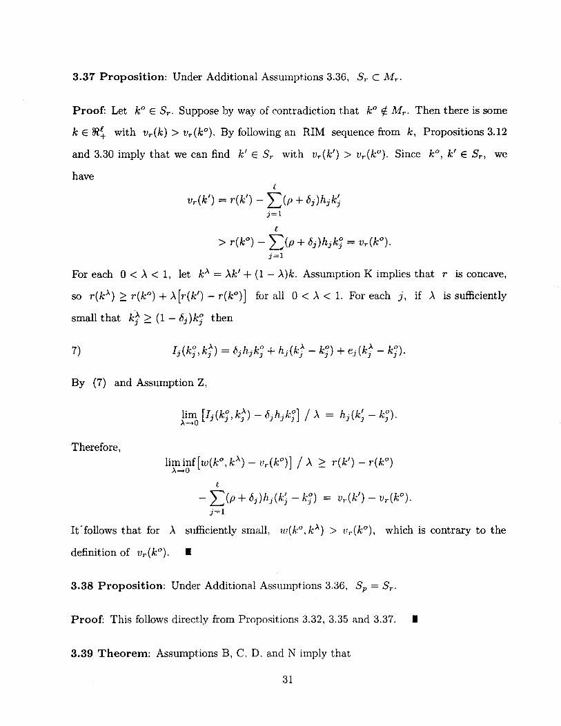
3.37 Proposition: Under Additional Assumptions 3.36, S1' c M 1·.

Proof: Let kO E Sr. Suppose by way of contradiction that kO tt. Mr. Then there is some

k E ~~ with vr(k) > vr(kO). By following an RIM sequence from k, Propositions 3.12

and 3.30 imply that we can find k' E Sr with vr(k') > vr(kO). Since kO, k' E STl we

have c

vr(k') = r(k') - I)p + bj)hjkj j=1

e > r(kO) - ''l)p + bj)hjkj = vr(kO).

j=1

For each 0 < A < 1, let kA = Ak' + (1 - A)k. Assumption K implies that r is concave,

so r(e·) ~ r(kO) + A[r(k') - 1'(kO)] for all 0 < A < 1. For each j, if A is sufficiently

small that k; ~ (1 - bj)kj then

7) [ ·(k·O kA) - ~·/l·ko+h·('··A kO)+e·(k·A k'O) J j' j - UJ OJ j J 1\') - j J j - j .

By (7) and Assumption Z,

Therefore,

t

- 2:(p + bj)hj(kj - k.i) = v,.(k') - vr(kO). j=1

It-follows that for A sufficiently small, w(kO,k A) > v,.(k°), which is contrary to the

definition of vr(kO). •

3.38 Proposition: Under Additional Assumptions 3.36, Sp = Sr.

Proof: This follows directly from Propositions 3.32, 3.35 and 3.37. •

3.39 Theorem: Assumptions B, C, D, and N imply that

31

a) for every residual income ma.ximizing sequence {kt}:o' d(kt, Sr) ----? 0; and

b) for every present value maximizing sequence {kt}:o' d(kt, Sp) ----? O.

Under the additional assumptions K and Z,

c) Sr = Sp.

In the absence of strict convexity assumptions, the common limit set need not be a

singleton. Under the assumption that the second derivative of the net revenue function is

strictly negative, Anctil (1994) shows that an RIM path converges to the unique stationary

capital level at an exponential rate. The multidimensional analog of Anctil's assumption

would be negative definiteness of D2r, which might be ensured by imposing smoothness

and curvature assumptions on the sets yi. It would also be necessary to assume that

the expansion cost functions are smooth and convex. The smoothness and curvature

assumptions would have to include boundaries in order to avoid the implausible assumption

that every activity requires the use of every internal commodity. In fact, the model should

allow the possibility that some activities are inactive at the stationary capital vector. In

any case, the assumptions needed to ensure the existence and negative definiteness of D2r

will be cumbersome at best in any model that, like the present model, strives for generality

in the class of allowable activity networks.

4. Activity-Based Costing and Residual Income Maximization

- We now turn to the design of a cost accounting system to support residual income

maximization. In contrast to the previous section, we focus on the choice of a single­

period plan, taking the previous capacity vector as given. The accounting system has

two principal elements. First, there are rules for computing the unit cost of the output of

each cost activity, including investment activities. Second, there are performance measures

that tell managers how to use the unit costs in selecting proposed actions. The specific

accounting system we will construct. termed the ABC mechanism, is an extension of the

32

ABC mechanism constructed by Jordan (1994). The ABC mechanism is a special case

of a general class of mechanisms called b'lLdget mechanisms. Several examples and a more

extensive discussion of budget mechanisms are given in Jordan (1994).

4.1 Definitions: Fix an initial capacity vector (kn~=l' an initial book-value vector

(J{f)~=1 E ~~, and capital policy parameters (p, (8i ):=1) E ~++ x (0, l)f. A firm, j, is

then specified by the remaining characteristics (Ii):=l and (yi):l+l' For an investment

activity i, in the interest of notational simplicity we will sometimes write yi to mean

the set yi (kf) defined in 2.2 above.

4.2 Budget Mechanisms: For each activity i, let Ai be a set, with generic element ai,

and let A = II~l Ai. For each i, let Q;: IIjii(Aj x pj) __ Ai, let /3i: Ai x pi __ pi,

and let 7ri: Ai x pi -- R. The function OJ is a reporting function, /3i is a budget

function, and 7ri is a performance rneaS'lLrement function. A budget mechanism is an

n-tuple (Ai, ai, /3i, 7ri)i such that the reporting functions satisfy:

Assumption A: For each plan (Yi)i E P such that for each j = 1, ... ,m, Yjj > 0 and

L:~=1 Yij ~ 0, there is at most one (ai) i E A that satisfies ai = ai (( aj, Yj) j#J for all

i = 1, ... ,no

4.3 Budget Equilibrium: Given a budget mechanism (Ai, ai, /3i , 7rd i , a budget equi­

librium for a firm f = ((Ii):=l' (yi)~~l+l) is an n-tuple (a;'Y;)i satisfying, for each

i = 1, ... ,n

i)

ii)

iii) Y; ma."'{imizes 7ri (a; .. ) on /3i (a; , pi) n yi.

4.4 Remarks: Assumption A embodies the restriction that the reports ai contain ac­

counting information only. Since the reports are determined by the proposed actions alone,

33

they are precluded from conveying information about marginal costs, marginal revenues, or

opportunity costs except to the extent that such information can be inferred from proposed

actions.

A budget equilibrium is formally a static concept, but it can be interpreted as an

outcome of a participatory budgeting process. Central management sends a report ai to

manager i, containing information about actions proposed by other managers. Manager

i then proposes an action Yi, which is modified by central management to fJi(ai, Yi).

Manager i, knowing ai and the budget function fJi, anticipates this modification

by proposing an action Yi such that f3i (a;. !Ji) E yi. so the action is feasible, and

Yi maximizes the performance measure 7r i ( Hi. /1.i (ai, . ) ) among such proposals. Central

management, in response to such proposals, sends new reports as dictated by the reporting

functions Qi, activity managers send new proposals in response to the new reports, and

so on. A budget equilibrium is a fi"{ed-point of this process.

One could model a budget process explicitly as an iterative or continuous-time ad-

justment process of this sort, but such a model would be artificially restrictive. In actual

participatory budgeting, there can be communication, perhaps informal or ad hoc, among

managers as well as between managers and central management, so manager i may obtain

information beyond the limits of the report ai, and may even coordinate proposals with

some other managers. We now define properties of budget mechanisms motivated by the

need to make the model robust to additional information and coordination.

4.5 Definitions: Let F denote it set of firms, that is. a set of n-tuples f =

((Ii)~=l' (yi)~=t'+l)' A budget mechanism (Ai, Qi, /3 i , 7ri)i is RI-compatible on F if for

each f E F, and each plan (Y;)i which is residual income maximizing for f given kO,

there is some (a;)i E A such that (a;, yni is a budget equilibrium for f.

For each plan (Yi) i E P, let 7r 0 ( (Yi ) J denote the residual income,

n f

7rO((Yi)i) = L !Jio-L(p+Di)[-YiO-(1-8dK f]. i=I'+I;=1

34

Given a budget mechanism (Ai, ai, tJi. 7rd i , define £(F) = {(ai, Yd i : (ai, Yi)i is a budget

equilibrium for some f E F}. The budget mechanism is RI-seeking on F if for each

(ai,Yi)i and (aLYDi E £(F), 7rO((Yi)i) ~ 7ro((yDJ if and only if 7ri(ai,Yi) ~ 7ri(a~.yD

for all i = 1, ... , n.

4.6 Remarks: RI-compatibility means that if a residual income maximizing plan were

somehow proposed, it would be accepted as the outcome of the budgeting process. Un­

fortunately, the informational limitations of the accounting reports (ai)i cause many

other plans to be equilibria as well. If the budget mechanism is RI-seeking, managers

who acquire additional information or who coordinate their proposals with others in order

to improve their measured performance will also raise the firm's residual income. The

RI-seeking property is an "open architecture" property that makes the budget mechanism

compatible with additional information and communication flows.

The concepts RI-compatible and RI-seeking are defined with reference to a set of

firms, F, in order to formalize an information constraint on the budget mechanism. The

size of the set F represents the extent of central management's ignorance of the char­

acteristics f = ((Ii):=l' (yi)~=Hl)' If central management knows these characteristics,

then F should be taken to be a one-point set {fl. In this case, the design of a budget

mechanism that supports residual income maximization is trivial. Let (y*i)i be a residual

income maximizing plan, and for each i. let tJi be the constant function !3i(') = y;. If. the set F is large, however, the inability to tailor the budget mechanisms to specific

elements in F will typically force an RI -compatible budget mechanism to admit many

budget equilibria that do not maximize residual income. The maximization condition 4.3

(iii) implicitly assumes that Yi is known by manager t, but we assume that these

characteristics are not known by other managers or by central management beyond the

knowledge that f E F.

The initial capacity vector, kO, the initial book-value, J{o, and the capital policy

35

parameters, (p, (bi)~=l) are fixed over F and thus assumed to be known by central

management, and may be used as parameters in the budget mechanism, as in the ABC

mechanism defined below.

4.7 The ABC Mechanism: Let Bi = {bi E ~1n: for some x E~, (x,bi ) E pi},

for i = 1, ... , n. Let C i = {Ci E ~nL : Cii = O} for i = 1, ... ,m, and C i = ~Tn for

i = m + 1, ... ,n. Define the report space Ai = ~ X Bi X C i , and A = II?=l Ai.

For each i = 1, ... ,n, the reporting function ai = IIj#i(Aj x pj) ~ Ai is given by

n e aiO - 2: YjO - 2: (p + bj )Kj, where

j=f+1 j=1 j#i j,ti

K j = (1 - bj)Kj - :tho for each j = L ... ,e;

if k = i;

min{O, - L:~:l Vjd if k =1= i and i > f; and Jr'

o otherwise.

(p + b ·)y·o J .1 if j::; £. j =1= i, and Yjj > (1 - bj)kj;

Cij - YjO + L:~=l Ckj Yjk

Yjj

o otherwise.

if £ < j :::; m, j =1= i, and Yjj > 0; and

The budget functions Pi: Ai X pi ~ pi are given by (1; ( (aiO, bi , Ci), Yi) = yf, where

yfo =YiO; and

yfj = max{ bij , Vi) }, j = 1, ... , m.

The performance functions 1fi: Ai x Pi ~ R are given by

36

and

i = .e + 1, ... , n,

where (x)+ denotes max{x, a}.

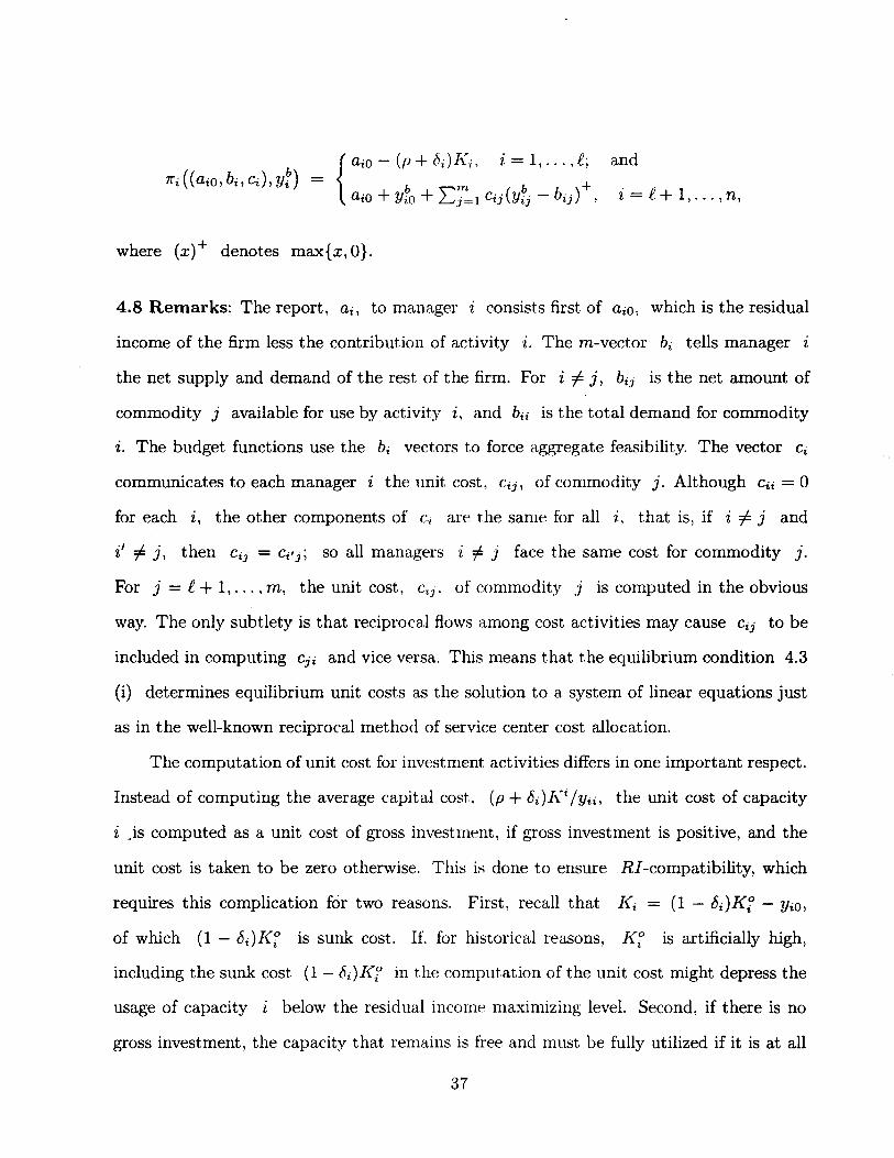
4.8 Remarks: The report, ai, to manager i consists first of aiD, which is the residual

income of the firm less the contribution of activity i. The m-vector bi tells manager i

the net supply and demand of the rest of the firm. For i i- j, bij is the net amount of

commodity j available for use by activity i, and bii is the total demand for commodity

i. The budget functions use the bi vectors to force aggregate feasibility. The vector Ci

communicates to each manager i the unit cost, Cij, of commodity j. Although Cii = a

for each i, the other components of Ci are the same for all i, that is, if i i- j and

if i- j, then Cij = Ci' j; so all managers i i- j face the same cost for commodity j.

For j = .e + 1, .... m, the unit cost, Cij. of commodity j is computed in the obvious

way. The only subtlety is that reciprocal flows among cost activities may cause Cij to be

included in computing Cji and vice versa. This means that the equilibrium condition 4.3

(i) determines equilibrium unit costs as the solution to a system of linear equations just

as in the well-known reciprocal method of service center cost allocation.

The computation of unit cost for investment activities differs in one important respect.

Instead of computing the average capital cost. (p + bi)I<i /Yii, the unit cost of capacity

i .is computed as a unit cost of gross investment, if gross investment is positive, and the

unit cost is taken to be zero otherwise. This is done to ensure RI -compatibility, which

requires this complication for two reasons. First, recall that I( = (1 - bdI<i - YiO,

of which (1 - bi)I<i is sunk cost. If. for historical reasons, I<i is artificially high,

including the sunk cost (1 - bi)I<i in the computation of the unit cost might depress the

usage of capacity i below the residual inCOlIH-' maximizing level. Second, if there is no

gross investment, the capacity that remains is free and must be fully utilized if it is at all

37

productive. Therefore activities that use capacity i must not be quoted a positive unit

cost when capacity i is freely available. For these two reasons, the unit cost of capacity i

is computed as the unit cost of gross investment. Unfortunately, this computation presents

a new difficulty because the denominator is problematic. The depreciation rate 8i is a

capital policy parameter chosen by central management. Ideally, as in Assumption I (3.2),

8i is also the rate of physical deterioration of capacity, but this ideal is rarely met in

practice. If 8i is too small, the denominator Yii - (1 - 8i )kf will be too small, again

raising the possibility that an overstated unit cost could depress capacity usage. For this

reason, in proving that the ABC mechanism is RI-compatible (Proposition 4.15) we will

need to assume that 8i is sufficiently large that Ii (ki, (1- 8i )kf) = 0 so that (1- 8dki

would be freely available.

Contrary to what one might expect, the performance measures 7ri do not use the

unit costs to compute a separate net income for each activity. Instead, the unit cost Cij

enters 7ri as a bonus for using less of commodity j than the available amount, yfj. This

provides exactly the same incentive to economize as would charging activity i the amount

Cij IYij 1 for the usage IYij I. In addition. it avoids a potential conflict of interest among

managers. Suppose managers i and j discover that residual income would increase

if some capacity that i was proposing to use was instead diverted to j. If i and j

have separate income statements, the result might be a reduction in i's net income and

an increase, by a greater amount, in j's net income. In this case, the budget mechanism

might fail to be RI -seeking.

The following proposition records the fact that the ABC mechanism satisfies As­

sumption A, and thus the definition of a budget mechanism.

4.9 Proposition: The ABC mechanism is a budget mechanism (4.2).

Proof: Let (Yi)i E P with Yii > 0 for all i = L .... m. and L~=l Yij 2: 0 for

each j = 1, ... , m. It is clear that for each i. aiO and bi are uniquely determined by

38

the reporting functions. Also, for each i, the unit cost Cij of each investment activity

j = 1, ... ,.e is uniquely determined. If one replaces YiO by YiO + L~=l CijYij for each

cost activity i = .e + 1, ... , m, then the unique determination of the unit cost Cij for

each i and each j = f + 1, ... , m follows exactly as in the proof of Proposition 5.3 in

Jordan (1994). •

4.10 Remarks: The following Proposition derives an equivalent but more transparent

statement of the ABC equilibrium conditions.

4.11 Proposition: Let (a;'Y;)i E rr~~l(Ai x Pi) satisfy a; = Qi((a;'Y;)ii:j) for all

i = 1, ... , n. Then (a;, yn is an ABC equilibrium given an initial capacity vector kO

if and only if

i)

ii) there is a vector p* satisfying pj = C;j

for each i, j = L ... , TTl and i =1= j,

and for each i = 1, ... ,e,

p; = 0 otherwise,

and for each i = e + 1 ..... m, m

Y;o + L pj y7j = 0: and j=l

p; = 0 if and only if Y~i = 0; and

3U

iii) for each i = 1, .... e. y; maximizes

and Vii + L Y;' i 2: 0; and i'#i

for each i = .e + 1, ... ,TI, y; maximizes m

ViO + Lpj Yij

j=l ji'i

subject to Yi E yi and

Vij + LV;'j 2: 0 for all j = 1, ... , m. i'#i

Proof: Feasibility is equivalent to the equilibrium condition Pi (ai, yn = Yi for all z

(4.3 (ii)) together with the requirement in 4.3 (iii) that /3 i (ai. yn E yi for all z.

Condition (ii) follows from the assumption that ai = O'i ((a;, yj) #J for all i, which

is equilibrium condition 4.3 (i). Condition (iii) is equivalent to equilibrium condition

4.3 (iii). •

4.12 Remarks: In 4.11 (ii), pi is the unit cost of commodity i. The notation pi is

used because, as 4.11 (iii) indicates. pi provides the same incentive effect as a transfer

price. However, the constraints in 4.11 (iii) are much more restrictive than the decision

set typically found in transfer price mechanisms. Each cost manager i must choose Vii

large enough to meet demand, and no manager i can use more than the available quantity

of any commodity j. For this reason, there are many ABC equilibria at volume levels

far below residual income maximization. In particular. the zero plan. Yi = 0 for all i, is

always an ABC equilibrium. Since C;; = () f()r t'very cost activity j. cost managers have

no incentive to exceed demand. Thus any iw"rt'ase in volullle H'quires some coordination

among managers, which makes the RI-seeking property indispensable.

40

We now proceed to prove that the ABC mechanisms is Rl-seeking. In addition

to some of the assumptions used in Section 3, we will need a version of downscaling for

investment activities. In addition, we will make a simplifying assumption that all cost

activities are active at a residual inCOlllf' maximum. When this assumption is not satisfied,

the proofs can be revised by dropping the inactive activities.

4.13 Assumptions:

AA (Active activities): If (yi)i is a residual income maximizing plan given kO then

yti > 0 for all i = 1, ... , m.

ID (Investment downscaling): For each i = 1, ... ,£, li(k?,O) = 0 and if x, x' ~ 0

satisfy li(k?,x) =0 and li(k?,x') >0 then ;z;'>:r and for each 0:::;>':::;1,

4.14 Remarks: Assumption ID implies that for each investment activity i, there is some

Xi ~ 0, possibly infinite, such that I;(k?,x) = 0 for all :r:::; Xi, and li(k?,') is strictly

increasing on the interval [Xi, 00). Thus kf - ;l:i is, implicitly, the amount of physical

depreciation, although we will not need to make the natural assumption that Xi:::; k?

As mentioned above, in order to prove that an RIM is an ABC equilibrium we rely

on some of the results of Jordan (1994). These results show that, given any allocation, a

proposed reduction in any input usage or output by any cost or revenue activity, leads to

determinable (perhaps zero) reductions in input use by all cost activities.

4.15 Proposition: Assume D. N (3.2), K (3.36), AA and ID. Let (Yi)i maximize residual

income given kO. Then there is a unique (an i E IIi Ai that satisfies a; = (}i (( aj , Y;) j:fJ for all i. If I i (k?,(1-8i )k?) = 0 for all i = 1, ... ,£, then (a;'Y;)i is an ABC

equilibrium given kO.

Proof: To prove the first assertion, for each i let a;o, b;, and C;j for j = 1, ... , e be given

by the definition of the reporting functions (}i (4.2). To obtain C;j for j = e + 1, ... ,m,

41

replace yio with yio+ EJ=1 cij Yij for each 'i = .e+ 1, ... ,m. Since (Yi)i is residual income

maximizing, Assumptions Nand D imply that E~=Hl Yij = 0 for all j = l + 1, ... , m,

and that there are no redundant activities (Jordan (1994, A.2)), so the required unit costs

exist by Lemma A.6 of Jordan (1994).

We now show that conditions (i) - (iii) of Proposition 4.11 are satisfied. The fact

that (Yi)i is residual income maximizing implies 4.11 (i) and that part of 4.11 (iii)

pertaining to investment activities. Proposition 4.9 implies 4.11 (ii), since yii > 0 for all

i = 1, ... ,m by Assumption AA. Hence, it suffices to show that for each i = m + 1, ... , n,

Yi solves the problem

Tn

maximize YiO + L P; Yij j=1

subject to Yi E yi

and Yij + L yT'j ;::: n, j = 1 .... , m. i'#i

By Assumption ID, Yio = 0 for each i ""n * 1, ... ,.e such that L."i'=l Yi'i > O. Hence,

without loss of generality, we can assume that for each i = 1, ... ,.e, Yii = - Ei'#i Yi'i'

Let i;::: m + 1, and let Yi satisfy the constraints in (*). By Assumption K, for each

0:::; A :::; 1, AYi + (1- A)Y; also satisfies the constraints in (*). Let Y; = AYi + (1 - A)y;

for some 0 < A :::; 1. First. suppose that i > m. Then by Jordan (1994, Lemma A.l1),

there exist numbers Aj, j = 1, ... , m satisfying

8) m

I)1 - Aj )Yij' = y~, - Uti' for all j' = 1. ... ,m. j=1

Therefore, by Assumption D, the plan

yi-l' V;, Yi+1"'" y~) is feasible. by 4.11 (ii) and (8), we have

m 111

9) Y;o - Y;o + L pi (yt - ;t/,) = L (yjo - YjO) j=1 j=(+1

42

l

+ I)p + bj ) [Yjo/(vij - (1 - bj)kj] (yij - yij)' j=l

Choosing A sufficiently small will make vt sufficiently near Yi and each Aj sufficiently

near 1 that for each j = 1, ... , £ with Y]j > (l-bj )kj we also have Y]j 2: yij > (l-bj )kj.

Then for each j = 1, ... ,£, Assumption ID and the fact t.hat Ij(kj,(I-bj )kj) =0 imply

that

10) l·(k'! y' .. ) < Y~o - (y~. - y'. ')Y~o/(v*' - (1 - b ·)kO) J J' JJ - J JJ JJ J JJ J J'

Consider the plan (yj') j obtained by replacing yjo by lj (kj , yj j) for each j = 1, ... , £

in the plan (yi) j" Then (10) implies that (vi') j is feasible, and together with (9),

that if Y;o - Yio + E';l Pj(Y& - Y;i) > 0 then the residual income from the plan (yi')j

exceeds the residual income from (y*k)j. Since vt = AYi + (1 - A)Yi, this contradiction

implies that YiO + E';l pj Yij :::; YiO + E~l~l pjv.'ij . This proves 4.11 (iii) for i 2: m + 1.

The case £ + 1 :::; i :::; m is nearly identical except that one uses Lemma A.13 of Jordan

(1994) instead of A.12 and obtains

8') m

L(1 - Aj)yjj' = Ai Y&' - yij" j' = 1, ... , l j=l j#i

instead of (8), and uses Ai Y; instead of v~ in the comparison plan (yi) j . •

4.16 Theorem: Let F* denote the set of firms satisfying Assumptions D, N, K, AA, and

ID, and for which li(ki, (1- bi)ki) = 0 for all i = 1, ... ,I!.. Then the ABC mechanism

is RI -seeking on F*.

Proof: Proposition 4.15 establishes that the ABC mechanism is Rl-compatible on F*.

Let (ai, yni be an ABC equilibrium for some firm in F*. Then Assumption Nand

D, together with 4.11 (iii) imply t.hat Y;j = bij for all i and all j = £ + 1, ... , n.

Assumption ID and 4.11 (iii) imply that for each j = 1, ... , I!. and each i, either

Y~· = b*· or c:J' = O. Therefore tJ tJ •

{ aio + (p + 8i )y7o

7ri(ai, yn = aio + uio otherwise.

43

if i :::; I!; and

4.17 Remarks: The downscaling assumptions, D and ID, are indispensable to the Rl­

compatibility of the ABC mechanism. More generally, the feasibility of down-scaling

is the kernel of linearity that is essential to the usefulness of activity-based costs. For

example, suppose that activity-based unit costs Pj, j = 1, ... ,m indicate that revenue

activity i, operating at the action :t)i. is unprofitable. That is, YiO + 2:7=1 Pj Yij < O. The implication is that the residual income of the firm would increase if revenue activity

i were dropped or at least down-scaled. Dropping activity i will actually save the cost

2:j:l Pj IYij I if each cost activity j can be down-scaled in response to the reduced demand

for commodity j. Otherwise actual cost savings may be less than the revenue, YiO, that

is lost by dropping activity i.

An investment activity j cannot be down-scaled beyond the capacity that would

remain in the absence of gross investment. say (1- dj )kj, where elj is the rate of physical

depreciation. Assumption ID implies that Pj. the unit cost of gross investment, represents

a lower bound on the savings that could be achieved by scaling capacity down to any level

between Yjj and (1 - dj)kj. The additional assumption that lj(kj, (1 - bj)kj) = 0

implies that bj 2: dj (book depreciation does not understate physical depreciation), and

that Pj is a lower bound on the potential cost reduction from cutting back to any level

between Yjj and (1 - bj)kj.

_ The convexity assumption, K, is needed in Proposition 4.14 to ensure that if manager

'/, can increase measured performance by moving from vi to some other feasible action

Yi, then any move from Y; in the direction of Yi is also feasible, as well as performance

improving. Small moves preserve the inequality Vjj > (1- bj )kj for investment activities,

so that the performance improvement indicated by the unit costs pj implies an actual

improvement in residual income. Hence. at it l'("sidual income maximum, the unit costs pj

are sufficiently accurate to avoid signalling fals(-' opportunities for improvement.

44

Unfortunately, the signals provided by the ABC mechanism are sufficiently coarse

to avoid signalling many real opport unities for improvement as well. However, there is a

"second best" optimality criterion that is satisfied by every ABC equilibrium. A plan that

cannot be improved by down-scaling any activity or activities was termed a semi-linear

optimum in Jordan (1994, 3.3), whert' it was shown that, in the absence of fixed costs,

every ABC equilibrium is a semi-linear optimum. It will be shown below that, despite

the presence of fixed costs, an analogous result holds in the present model.

The definition of semi-linear optimality with respect to residual income (RISLO),

which is stated formally below, requires some care. The ABC costs give activity managers

the illusion that if capacity usage is reduced, capacity costs will be reduced proportionately.

Accordingly, RISLO is based on a definition of downscaling that incorporates this illusion.

In particular, the definition permits capacity downscaling, with capacity valued at its

ABC cost, rather than historical cost. That is. capacity is valued the unit cost of gross

investment, or zero in the absence of gross inv~stment. Proposition 4.19 states that every

ABC equilibrium is an RISLO. Thus, even though potential cost savings over stated

by including illusory reductions in the interest and depreciation charges for capital, the

residual income of an ABC equilibrium cannot be increased by downscaling.

4.18 Definition: Given a plan (yi)i' define J{* E?R~ as

{

-yjoyjj

J{; - yjj - (1 - 8j )kj

o otherwise, for all j = 1 .... , .l.

if and

The plan (y;)i constitutes a semi-linear optimum with respect to residual income (RISLO)

if the problem

45

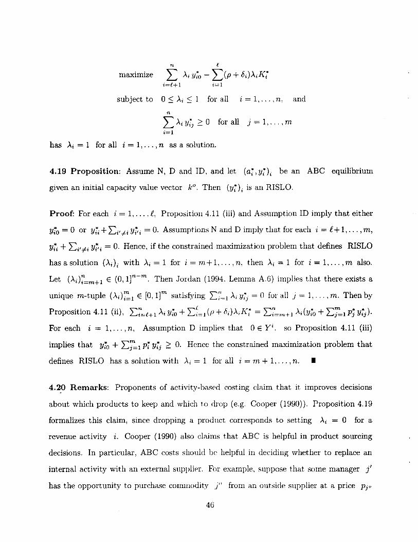
n I'.

maximize L: Ai yio - L:(p + 8i )AJ<t i=I'.+1 i=1

subject to 0:::; Ai :::; 1 for all i = 1, ... , n, and

n

L: Ai Yij ~ a for all j = 1, ... , m i=1

has Ai = 1 for all i = 1, ... ,n as a solution.

4.19 Proposition: Assume N, D and ID, and let (ai, yni be an ABC equilibrium

given an initial capacity value vector kO. Then (yni is an RISLO.

Proof: For each i = 1, ... , C, Proposition 4.11 (iii) and Assumption ID imply that either

yio = a or Yii + 2:i'#i y;'i = O. Assumptions Nand D imply that for each i = f+ 1, ... , m,

yii + 2:i'#i yi'i = O. Hence, if the constrained maximization problem that defines RISLO

has a solution (Ai), with Ai = 1 for i = m+ L ... , n, then Ai = 1 for i = 1, ... ,m also.

Let (Ad7=m+1 E (O,lr-m. Then Jordan (1994. Lemma A.6) implies that there exists a

unique m-tuple (Ai)::1 E [O,IJm satisfying 2:;'=1 Ai Yij = () for all j = 1, ... ,m. Then by

Proposition 4.11 (ii), 2:7=f+l Ai y·io + 2::=1 (p + 8i )AJ'(i = 2:~=m+l Ai (Yio + 2:;:1 pj yij )·

For each i = 1, ... , n, Assumption D implies that a E yi, so Proposition 4.11 (iii)

implies that yio + 2:7=1 pi Yij ~ O. Hence the constrained maximization problem that

defines RISLO has a solution with Ai = 1 for all i = m + 1, ... , n. •

4.2.0 Remarks: Proponents of activity-based costing claim that it improves decisions

about which products to keep and which to drop (e.g. Cooper (1990)). Proposition 4.19

formalizes this claim, since dropping a product corresponds to setting Ai = a for a

revenue activity i. Cooper (1990) also claims that ABC is helpful in product sourcing

decisions. In particular, ABC costs should be helpful in deciding whether to replace an

internal activity with an external supplier. For example, suppose that some manager j'

has the opportunity to purchase commodity j" from an outside supplier at a price PjO

46

per unit. If the ABC unit cost of activity jO, Pjo, exceeds PjO, then Propostion 4.11 (iii)

implies that manager j' will switch to the outside supplier. Formally, manager j' will

change his or her proposed activity vector from Y;' to

Proposition 4.21(i), below, states that the ABC unit cost, Pjo, accurately represents the

cost savings that would be achieved by downscaling activity yo, subject to the same

qualification about capacity downscaling as in Proposition 4.19. Assertion (ii) records the

fact that at an ABC equilibrium, only unattractive outsourcing opportunities can remain

untaken.

4.21 Proposition: Let (a;, yi)i be an ABC equilibrium, and for each i = 1, ... , m ,

let pi be given by Proposition 4.11(ii) and assume that Yio < 0. For some jO ~ m, let

PjO ~ 0, and for some j' >.e with yjl jO < 0, let

For each i =1= j', let Yi = Yi. For each i = 1, ... , m, let ° ~ Ai ~ 1 be the

unique coefficient such that for all j = 1 .... , m, 2::1: 1 AiYij + 2:~m+1 Yij = 0. Let

z = 2:7:l+1 AiYio + 2:~m+1 YiO - 2::=1 (p + l5i )AJ<i, where I<t is given by Definition

4.18, i = 1, ... , e. Let z* = 2:::£+1 Yio - 2:1=1 (p + l5i )Iq. Then

i) z - z* = (pjo - pjo)IYjljOI; and

ii) _ if Yj' E yjl then PjO ~ pjo.

Proof: Assertion (i) follows directly from Jordan (1994, Lemma A.11) if j' > m, and from

Jordan (1994, Lemma A.13) if j' ~ Tn. Assf'rtion (ii) follows directly from Proposition

4.11 (iii). •

4.22 Remarks: The outsourcing result is subject to a subtle but substantive limitation

in the presence of reciprocal relationships among cost activities. Suppose that activity j'

47

is a cost activity. Then, in the notation of the Proposition, it can happen that Ajl < 1.

This means that the downscaling of the outsourced activity, jO, has indirectly lessened

the demand for commodity j'. In particular, the amount of commodity f that will be

purchased externally is not IY;, jO 1 but the lesser quantity Ai' Iy;' jO I. Thus the definition

of z embodies the assumption that the external price PjO per unit of commodity f is

unaffected by downscaling the quantity purchased.

Thus the ABC mechanism provides good support for weeding out unprofitable prod­

ucts and outsourcing inputs that can be obtained externally at lower cost. Of course,

in evaluating these decisions, only tll<" implicaJions of downscaling the existing plan are

considered. If some cost activity has sharply decreasing returns to scale, a reduction in

the scale of output would result in more than proportional cost reduction. Such nonlinear

opportunities are not revealed by ABC unit costs.

4.23 Relation to recent literature: An important recent addition to the theoretical

literature on the activity-based costing of fixed resources is given by Banker and Hughes

(1994). Banker and Hughes formulate a two-period model in which the firm chooses

fixed levels of certain inputs in the first period, and produces to meet demand in the

second period. The production technology is Leontief up to capacity levels set by the fixed

inputs, beyond which costs increase at a constant but higher marginal cost. The demand

curve facing each of the firm's products is linear, so revenue functions are quadratic. The

prqd uction technology is known by a production manager. and the demand functions are

known by a marketing manager. These aspects of the Banker and Hughes model can

be included in the activity model of the present paper as a special case (Banker and

Hughes point out that their demand linearity assumption can be dropped, but their use of

first-order conditions would presumably still require the concavity of revenue functions).

However, the focal feature of their mudd is the assumption that each demand curve is

perturbed by an additive stochastic shock that. is not observed until after the fixed inputs

48

are in place and the product prices have been set. They assume that the demand and

cost parameters are such that the firm will always find it profitable to meet the entire

realized demand. Nonetheless, they obtain the surprising result that if the fixed inputs

are chosen to maximize ex ante expected profit, then the ABC costs generated by the

Leontief technology in the region below the fixed-input capacit.ies represent "economically

sufficient" information about the production technology for the marketing manager to

choose the expected-profit maximizing product prices.

The Banker and Hughes result suggests the possibility that the nonstochastic model of

the present paper might be extended t.o allow the firm's characteristics to include random

disturbance terms, and to replace the residual income performance measure with expected

residual income. Unfortunately, Banker and Hughes note that the production manager's

choice of the expected-profit maximizing fixed-input levels requires the knowledge of the

probability distribution of the demand shocks. Work currently underway by Jordan and

Dingbo Xu indicates that even in a two-activit.y, two-period model, expected-profit maxi­

mization can require an infinite amount of communication between managers.

Accounting Horizons has published a series of papers for educators and practitioners

on activity-based costing, some of which explicitly address the treatment of fixed costs.

Malcom (1991) and Mak and Roush (1994) recommend that the costs of individual activ­

ities be decomposed into variable and fixed (lVIalcom uses the term "sticky") components,

which Kaplan (1994) regards as a potentially useful refinement. The present paper, in

cO.ntrast, posits a sufficiently fine-grained act.ivity model that fixed and variable costs are

separated into different activities. In particular, the acquisition of each fixed resource is

a separate investment activity. Activities that use fixed resources are treated as though

their costs were entirely variable, although our downscaling assumption (Assumption D)

is much weaker than the proportionalit.y assumption that accompanies most analyses of

variable cost. Indeed, a major goal of this paper is to show that activity-based costs can

be useful even when the proportionality assumption is violated.

49

Cooper and Kaplan (1992) and Kaplan (1994) recommend a specific calculation of the

unit cost of a fixed resource. Their examples involve only contemporaneous expenses, so

their cost calculations do not involve interest charges. More importantly, they recommend

that the budgeted unit cost of a fixed-resolU'Ce be computed by dividing the total budgeted

cost of the resource by its "practical capacity" (e.g., Kaplan (1994, p. 106)). In the notation

of the present model (including the interest charge), this would yield:

CK)

taking (1 - bj)kj as a measure of practical capacity in the absence of gross investment.

The unit capacity cost in the present model (see 4.11 (ii)) is:

AJM) {

-(p+bj)yjo

yjj - (1 - bj)kj

o otherwise.

if and

The major distinction between the two formulae lies in the treatment of excess capacity

(Yij ~ (1- bj )kj). In this case, the capacity expense, (p+ bj )Kj , which is charged against

residual income, is a purely sunk cost, and the economic cost of capacity is zero. Nonethe-

less, (CK) is positive in this case. If the formula (CK) were used in the ABC mechanism,

Proposition 4.15 and Theorem 4.16 would no longer hold. A residual income maximum

could fail to be an ABC equilibrium because activity managers could be discouraged from

fully utilizing an economically cost less reSOlUTe. Any cost system that allocates the cost

of fixed resources risks overstating the potential cost savings from dropping products or

outsourcing activities. As mentioned in Section 4.17, the ABC mechanism of the present

paper is no exception. The capacity cost given by (AJ:~vI) keeps the overstatment of cost

savings below the point of discouraging the optilIlal use of the resource.

4.24 Example: The relation between ABC equilibrium and residual income maximiza-

tion can be illustrated by a simple quadratic example. Suppose the firm consists of a single

50

investment activity and a single reVt-~nue act.ivity. Where there is no risk of confusion, we

will suppress the activity subscripts. The investment function J is given by

which satisfies Assumptions C, I, Z and ID. Hence the set of feasible actions for the

investment activity is given by

For the revenue activity, the feasible action set is given by

where , is a positive parameter that will be varied to create different versions of the

example. Hence y2 satisfies Assumpt.ions B C, D. Nand K. As long as kO > 0,

Assumption AA is satisfied, so the finn satisfies all of tlw assnmptions of Sections 3

and 4. A plan (!JIO, Yn; !J20, !J2d is feasible for the firm given an initial capacity kO if

(YlO, Yn) E yI(kO), (Y20, Y2d E y2 and Yn + Y21 ~ 0.

Given an initial book-value ]{O, a plan (YIO, Yn; Y20, Y2d results in the new book

value

K = (1 - 8)J{O - YIO,

and the residual income

RJ = Y20 - (p + 8)K.

-Since ,> 0, the choice of a residual income maximizing plan reduces to a single variable

problem, because an RI maximizing plan must satisfy Yn + Y21 = 0, YIO = -J(kO, Y11)

and Y20 = ,( -JJ2d - (U21)2, provided that. h:o is not so large that excess capacity is

optimal (i. e., (1 - (5)h:o ::; ",//2). Let k denote thp common value of Yll and -Y21'

Viewing RI as revenue minus cost, \ve can express the marginalr'evenue as

A1R(k) = "( - 2k,

51

and the marginal cost as

{

(p + b) [120 + lO(k - kG)] A-1C(k) = (p + 15)120

°

if k > kG; if (1 - b)kO < k :::; kG; ifk< (l-b)ko.

In this example, Proposition 3.35 implies that the stationary capacity, kS can be obtained

as the unique solution to the equations kO = kS and A1 R(kS) = A1C(kS), which yield

kS = ,- (p + b) 120. 2

Given an initial capacity kG, the residual income maximizing capacity satisfies

k = sup{k : A-1R(k) 2: MC(k)},

which can be expressed more explicitly by distinguishing three cases depending on the size

of the initial capacity relative to the stationary optimum:

if kO < kS;

if (1 - b)kO :::; kS :::; kG; if kS < (1 - b)kO :::; ,/2.

In the first case, the firm is growing toward k S; in the second case, the firm has reached

the stationary optimum; and in the third case, the firm is contracting toward kS via

depreciation while continuing t.o produce at full capacity.

The ABC mechanism in this example can be described as follows. Given a proposed

plan (iho,Yll;iho,ihd, manager 1 receives the report (alO,bll,cll) = (:ii20,-Y21,0),

which parameterizes the budget function ,Bd(alO,bll,cll), (YlO,Yll» = (yro,yrl) as

and the performance function

where J( = (l-b)J(o -yro. :Manager 1 is constrained to choose a proposal (YlO, Yll) that

satisfies the feasibility requirement that (urn.!A t> E 1"1 (kO). As a result, Manager 1 will

52

respond by simply meeting Manager 2's proposed capacity demand (Yll = -Y21) and

reporting the minimal investment cost needed to achieve that capacity (YlO = - I(kO, Yll)).

Manager 2 receives the report (a20, b21 , C21), given by a20 = -(p + b)K, b21 = -Yll

and

{

(p + b)ylO

_ oYU - (1 - b)ko

otherwise.

if Yu - (1 - b)kO 2 0; and

and the performance function

Manager 2 must choose (Y2o, Y21) so that (y~o, y~ 1) E y2. As a result, Manager

2 will respond by choosing -Y21 - max{k : k :s; -b21 and MR(k) 2 C2t}, and

reporting Y20 = '(-Y2d - (Y2d 2. Hence, any proposed plan Ciho,Yll;Y20,Y2d that

satisfies Yll = -Y21, YlO = -I(ko,Yll), Y20 = ,(-fhl) - (fj2d 2 and MR(-Y2d 2 C21

is an ABC equilibrium. Let k* denote that common value of Yll and -Y21. Then

the key equilibrium condition, AI R(k*) 2 C21, reduces to

ABC) if kO < k*; if (1 - b)kO < k* :s; kO; if k* :s; (1 - b)ko.

Any k* that satisfies (ABC) is an ABC equilibrium level of capacity usage.

The inequality (ABC) allows a wide range of equilibria. Since the budget functions

do not allow Manager 2 to increase capacity unilaterally above the level proposed by

Manager 1, the mechanism can get stuck at low output levels. However, in this case,

M R( k*) is well above the reported capacity cost C21, so one might expect Manager 2,

in the interest of increasing 7r2, to commnnicate directly with Manager 1 and attempt to

53

elicit an increase in Yu. Since the ABC mechanism is RI-seeking (Theorem 4.16), such

an attempt can succeed. There are also ABC equilibria with capacity levels above the

residual income maximum k. The investment function J(ko,.) is strictly convex above

kO, reflecting expansion costs, so the average cost of gross investment in this region is less

than the marginal cost. Therefore there can be ABC equilibria satisfying MC(k*) >

MR(k*)? C21. AlthoughManager 1 knows AIC(k*), thereport (alQ,bu,cu) contains

no revenue information, so neither manager has any information suggesting that k* is

too large. This problem can be mitigated by extending the budget mechanism to report

average revenue, iho/k*, to Manager L and allowing Manager 1 to reduce capacity

below -Y21 subject to a performance penalty equal to average revenue times the amount

of the shortfall. This will prevent AIC(k*) from exceeding average revenue. However, if

revenue is a strictly concave function of k*, as in the present example, average revenue

exceeds marginal revenue, so there will continue to be a range of ABC equilibria with

MC(k*) > AIR(k*), that is, k* > A:. Such an extension of the ABC mechanism is

constructed in Jordan(1994, Section 6) in a single-period model without fixed costs.

Suppose that Cn is calculated Hot as the unit cost of gross investment, but as the

unit cost of practical capacity, as suggested by Cooper and Kaplan (1992) and Kaplan

(1994). The formula 4.23 (CK), applied to the present example, yields

, (p + 8)J< c21 = ,

'T1Ia;r{Yll' (1 - 8)ko}

and the equilibrium condition becomes AIR(k') 2: (p+8)K/max{k', (1 - 8)kO}. Assume

that KO = 120ko, i. e .. that the initial book value is not distorted by previous expansion

costs. Then the equilibrium condition can be written

ABC') M R(k') > {(p + 8)[120 + S( k' ;/,0)2 J

- (p+8)120 if kO < k'; if k' :::; kO.

Comparing the equilibrium conditions (ABC) and (ABC') indicates that c~l is lower

than C21 if the firm is expanding, higher if tlw firm is contracting, and the same if capacity

is stationary. In general, C21 approximates .HC as \vell or better than C~l'

54

The comparison of equilibria is illustrated in the following two numerical cases. In

both cases we retain the assumption that ](0 = 120ko, and also set b = 0.4 and

p = 0.1. First, let, = 150, and kO = 100. These values specify a contractionary

case, with kS = 45 < 60 = (1 - b)ko. The residual income maximum is k = 60, with

M R(60) = 30. The residual income IlHL"'(imum is the largest ABC equilibrium, but since

C~l = 120, the largest ABC' equilibrium is the stationary optimum, kS• Thus if the

unit cost of practical capacity is used in place of C21, which is zero in this case, then 15

units of cost less capacity will remain unused.

To specify an expansionary case, set ,= 300 and kO = 50. Then k S = 120 > 30 =

(1 - b)kO, and the residual income maximum is k = 70. In this case, MR(k) = 160 >

C21 = 85 > C~l ~ 74, so the residual income maximum is supported as an equilibrium by

both costing methods. The largest ABC equilibrium is k* ~ 88.4, at which M R(k*) =

C21 ~ 123 > C~l ~ 102. It follows h:om the inequality that (ABC') permits larger

equilibrium capacities with correspondingly lower residual income. The largest ABC'

equilibrium is k' ~ 94.1, at which A1R(k') = C~l ~ 112 < C21 ~ 136. Again, C21

provides the better approximation to marginal cost.

4.25 Asset Sales: The ABC mechanism directs cost activity managers to meet the

demand for their output at the minimum cost. As illustrated by the previous example,

the manager of an investment activity receives no revenue information, and has no means

to. compare the cost of providing capacity with the revenue generated by its use. Only

revenue activity managers are in a position to make such comparisons. As a result, the

sale of capital goods by investment managers is outside the scope of the present model.

Of course, such sales as arise incidentally in the course of replacing old equipment with

new create no conceptual or formal difficulties. Any revenue realized in the sale of an

old drill-press is subtracted from the cost of the new drill-press in calculating YiO, in

accordance with the conventional accounting treatment of similar asset exchanges.

55

The sale of assets for the purpose of earning revenue, as opposed to minimizing re­

placement cost, conflicts with our sign convention that YiO:::; O. The sign convention

and the more explicit restriction in Section 3 that capacity can decrease only through

depreciation are imposed largely for simplification. The opportunity to sell an asset, if

anticipated at the time the asset is acquired, reduces the extent to which its cost is fixed

and can affect its capitalization. We have avoided such complications in order to focus on

fixed costs. It is likely that only a minor modification of the model would be required to

encompass the unanticipated sale of unused capacity. However, the sale of capacity that

would otherwise be used requires an opportunity cost calculation that is not supported by

the ABC mechanism.

The asset that seems least suited to our model of investment activities is land. Since

land does not depreciate, gross investment occurs only when new land is acquired. Hence,

under the ABC mechanism, the unit cost of land is positive only when new acquisitions

are budgeted. The zero depreciation rate also excludes land u'om the dynamic analysis

in Section 3. If the firm's initial land holdings exceed their stationary optimal level, the

stationary optimum cannot be achieved in a model without asset sales.

The ABC mechanism is refined in .Jordan (1994, Section 6) by using budgeted

revenues to construct a measure of opportunity cost. The refinement, called the ABOC

mechanism, improves performance by enabling managers to reject many of the suboptimal

ABC equilibria. However, the cost calculations are considerably more intricate and,

n~dless to say, unconventional. An extension of the ABOC mechanism to the present

model could provide capacity costs in the absence of gross investment that are positive

but not disfunctional, and might provide at least limited support for the disposal of assets

that can be sold for greater revenue than is generated by their use.

5. Stationary Equilibria

A stationary ABC equilibrium (aT, y7); is an equilibrium with the additional

56

property that kf = Yii for each investment activity i, so the plan remains constant

over time. Stationary equilibria deserve special attention for two reasons. First, Section 3

showed that a sequence of residual income maximizing plans is asymptotically stationary.

Second, the capital valuation equation, Kf = (1 - D;)K~-l - yfo, drives Kf to the

stationary book-value, Kt = -Yiol Di, if Di > 0 and Y;o = Yio for all t. This implies

that the average cost of gross investment is equal to the average book-value of capacity, so

the ABC unit cost pi is given by pi = (p + bi)Ki 1y.7;. This fact, which is recorded as

Proposition 5.2, is independent of any relation between the depreciation rate bi and the

physical depreciation of capacity.

Proposition 5.3 states that, under the hypothesis of Proposition 4.15, a stationary plan

that maximizes residual income is also a stationary ABC equilibrium. Proposition 5.5

states that a stationary equilibrium, together with the corresponding stationary book value

vector, constitutes a semi-linear optimum.

5.1 Definitions: An n-tuple (ai, yn; is a sta.tiona.'ry ABC equilib'Num if (ai, yi)i is

an ABC equilibrium for the initial capacity vector (Y.7J:=1' A plan (yi)i is a stationary

residual income maximize?' if it maximizes residual income given the initial capacity vector

(yii):=l'

5.2 Proposition: Let (ai, yi)i be a stationary ABC equilibrium. For each investment

activity i = 1, ... , e let pi be given by 4.11 (ii), and let

Kt { -yiolb i

- 0 otherwise,

if and

Then pi yii = (p + bi)Ki for each i = 1, .. , . t.

Proof: The result follows from 4.11 (ii) and the definition of Kt, together with the

fact that kf = yii' •

5.3 Proposition: Assume D. N. K, AA, and Dr. Lt-'t. (Y.;)i be a stationary residual

57

income maximizer. If, for each i = 1, ... , e, Ii (Yii' (1- bdYii) = 0, then there is a unique

(ani E ITi=l Ai such that (ai, yi)i is a stationary ABC equilibrium.

Proof: This follows immediately from Proposition 4.15 and Definition 5.1. •

5.4 Definition: A plan (yi)i is a long-Tun semi-linear optimum (LRSLO) if (yi)i is an

RISLO for the initial capacity vector kO = (viI' ... , Yel)'

5.5 Proposition: Assume N, D, and ID, and let (ai, yi)i be a stationary ABC equi­

librium. Then (yi)i is an LRSLO.

Proof: This follows directly from Proposition 4.19 and Definition 5.4. •

6. Conclusion

This paper provides an integrated model of activity-based costing and performance

measurement in an information ally decentralized participatory budgeting process. Fixed

costs are included by incorporating investment decisions in the budgeting process. The

objective of the budgeting process each period is the maximization of residual income (eco­

nomic value added). Residual income maximization is rigorously justified as an asymptotic

approximation to discounted cash flow maximization, extending an earlier result of Anctil

(1994).

The ABC costs support residual income maximization in the sense that a residual

income ma .. 'Cimum is an equilibrium of the budget process. However, since the model

permits nonlinear production technologies, ABC costs are not generally equal to the true

marginal costs, so there are also budget equilibria that are not residual income maxima.

For this reason, the ABC budget mechanism is shown to have two additional properties.

First, the mechanism has the "open-architecture" property that if activity managers use

additional information or collude in the budgeting process to increase their measured

performance, then they will also increase the firm's residual income. Second, although

58

the budget mechanism does not enforce residual income maximization, it has the "second­

best" property of enforcing the dropping of unprofitable products, in the following sense.

Suppose that dropping a particular product would result in a revenue loss that is less

than the cost savings that would be obtained by linearly downscaling the expenses and

activities formerly needed by that product to the maximum extent consistent with meeting

the needs of the remaining products. Then that product will not be produced in a budget

equilibrium. In the same sense, the budget mechanism also enforces the outsourcing of

activities that can be more cheaply obt.ained externally. Of course, the ABC costs are

not sufficiently accurate to reveal opportunities for super-linear cost savings. These results

extend analogous results obtained by Jordan (1994) in a single-period model that excludes

fixed costs.

The principal remaining limitation of the model is that it is entirely nonstochastic.

Uncertainty in the sense of ignorance is plausibly represented by our assumption that an

activity manager has no direct knowledge of the characteristics of other activities. The open

architecture property ensures that additional knowledge, if acquired, will be used in the

interest of the firm. However, uncertainty in the sense of known probability distributions

governing market or technological characteristics is excluded from the model. Even in a

two-period model with stochastic activity characteristics, the complexity of expected profit

maximization makes a theory of accounting support problematic. It appears unlikely that

a model along the present lines could be attempted unless a practical heuristic can be

found to play the same role for expected profit maximization that residual income plays

for present value maximization.

59

References

Anctil, R., (1993), "Capital Budgeting Using Residual Income Maximization", Review of

Accounting Studies, forthcoming.

Banker, RD., and J.S. Hughes, (1994), "Product Costing and Pricing", Accounting Review,

69, No 3, pp. 479-494.

Christensen, J. and J. Demski, (1992), "The Classical Foundations of 'Modern' Costing",

mimeo.

Cooper, R (1990), "Cost Classification in Unit-Based and Activity-Based Manufacturing

Cost Systems", Journal of Cost Management for the Manufacturing Industry, Fall,

pp. 4-13.

Cooper, R. (1992), "Activity-Based Costing for Improved Product Costing", in Handbook

of Cost Management, 1993 Edition, B. Brinker (ed.), Warren Gorham Lamont.

Cooper, R, and R Kaplan (1992), ·'Activity-Based Systems: :Measuring the Cost of

Resource Usage", Accounting HO'l'izons, 6, No 3, pp. 1-13.

Eisner, R. and R Strotz, (1963), "Determinants of Business Investment," in Impacts of

Monetary Policy, Commission on Money and Credit, Prentice-Hall, Engelwood,

N.J.

Jordan, J.S., (1994), "Management Accounting in Activity Networks", mimeo.

Kaplan, R, (1994), "Flexible Budgeting in an Activity-Based Costing Framework," Ac­

counting Horizons, 8, No 2, pp. 104-109.

Lefshetz, S., (1977), Diffe1'ential Equations: Geometric Theory, Dover Publications Inc.,

New York.

Mak, Y.T. and M. L. Roush, "Flexible Budgeting and Variance Analysis in an Activity­

Based Costing Environment," Accounting Horizons, 8, No 2, pp. 93-103.

Malcom, R.E. (1991), "Overhead Control Implications of Activity Costing," Accounting

Horizons, 5, No 4, pp. 69-78.

Noreen, E., (1991), "Conditions under which Activity-Based Cost Systems Provide Rele­

vant Costs", Journal of Mangement Accounting Research, Fall, pp. 159-168.

60

Sargent, T. (1979), Macroeconomic Theo'ry, Academic Press, New York.

Stewart, G.B., (1991), The Quest for Val'ue, Harper Business, New York.

Stokey, N.L., and R.E. Lucas, Jr (1989), Recursive Methods in Economic Dynamics, Har­

vard University Press, Cambridge, Mass.

61