ACTIVITY COEFFICIENTS AND PLATE EFFICIENCIES IN DISTILLATION OF

MULTICOMPONENT AQUEOUS SOLUTIONS

PROEFSCHRIFT

TER VERKRIJGING VAN DE GRAAD VAN DOCTOR IN DE LANDBOUWWETENSCHAPPEN

OP GEZAG VAN DE RECTOR MAGNIFICUS, IR. F. HELLINGA, HOOGLERAAR IN DE CULTUURTECHNIEK, TE VERDEDIGEN TEGEN BEDENKINGEN

VAN EEN COMMISSIE UIT DE SENAAT DER LANDBOUWHOGESCHOOL TE WAGENINGEN

OP 18 JUNI 1969 TE 16.00 UUR

DOOR

S.BRUIN

H.VEENMAN&ZONEN N.V.-WAGENINGEN 1969

/r/i — lot/Of-^9

• IBLIOTHEEK. DEIt

lANDEOUWHOGESCHOOfc WAGENINGEN.

Aan mijn ouders

,j/J0?2O!, W)

S T E L L I N G E N

I Het is opmerkelijk dat de concentratie afhankelijkheid van activiteits-

coefficienten voor binaire systemen nauwkeuriger wordt voorspeld met de door ORYE gemodificeerde WILSON vergelijkingen wanneer slechts het enthalpische gedeelte wordt gebruikt.

WILSON, J. Am. Chem.Soc. 84,127-133,1964; ORYE, Ph-D dissertation, University of California, Berkely, 1965; Dit proefschrift.

II Tegen de verklaring voor het separatie effect in een isotherme Clusius-Dickel

kolom, welke LUIKOV C.S. geven zijn ernstige bezwaren in te brengen.

LUIKOV, Int. J. Heat and Mass Transfer 3,167-174,1961; LUIKOV and MIKHAILOV, Theory of Energy and Mass Transfer, Pergamon Press, 1965.

Ill Toepassen van WKB-approximatie, als voorgesteld door SELLARS, is niet nood-

zakelijk voor het verkrijgen van een eenvoudige benaderingsformule voor de ho-gere eigenwaarden in het klassieke Graetz-Nusseltprobleem voor vlakke platen.

SELLARS, KLEIN, TRIBUS, J. Heat Transfer 78, 441^*48, 1956; ABRAMOWITZ, STEGUN, Handbook of Mathematical Functions, Dover, 1964; INCE, Ordinary Differential equations, Chapt. 7,11, Dover, 1956.

IV De vergelijkingen van NIKOLAEV C.S. voor radiale, tangentiale en meridionale

snelheidsprofielen voor stroming van vloeistoffilms over een roterend conisch oppervlak, kunnen door eenvoudiger vergelijkingen worden vervangen, die even nauwkeurig zijn.

NIKOLAEV C.S., Int. Chem. Eng. 7(4), 595-598,1967.

V Tegen de analytische oplossing van het gekoppelde stelsel differentiaal-

vergelijkingen voor gecombineerd stof- en warmtetransport tijdens contact drogen van een laag vochtig materiaal zoals gegeven door MAKOVOZOV zijn bezwaren in te brengen.

MAKOVOZOV, Zh. Tekn. Fyz. 25,2511-2525,1955; BRUIN, Int. J. Heat and Mass Transfer 12,45-59,1969.

S. BRUIN Wageningen, 18 juni 1969.

VI Bij aromaconcentratie door rectificatie is het, in tegenstelling tot de bewering

van ROGER en TURKOT, gewoonlijk irrelevant of, volgens het [x,y] diagram, al dan niet heterogene minimum azeotropen gevormd kunnen worden.

ROGER, TURKOT, Food Technology 19,69-72,1965.

VII De'crowding coefficients', zoals gedefinieerd door De Wit voor het beschrij-

ven van concurrentie tussen twee plantensoorten die simultaan werden uitge-zaaid op een veld, zijn formeel niet analoog met de activiteitscoefficienten in de thermodynamica van mengsels. Daarentegen kan men de 'crowding coefficients' in verband brengen met het 'surface excess' bij monomoleculaire adsorptie aan een grensvlak van gas- en vloeistofphase.

DE Wrr, On Competition, Versl. Landbouwk. Onderz. 668,1960; GUGGENHEIM, Thermodynamics, 5th Ed., North Holl. Publ. Cy, 1967.

VIII De methode van VAN WUK voor het bepalen van de temperatuurverefTe-

ningscoefficient, waarbij temperatuur-registrogrammen worden omgezet in Laplace getransformeerden, verdient meer aandacht.

VAN WIJK, BRUIJN, PhysicaiO, 1097-1108,1964.

IX In het studieprogramma voor de A-richting van de richting Levensmiddelen

technologie aan de Landbouwhogeschool dient het vak fysische transport-verschijnselen te worden opgenomen.

X De juistheid van de opmerking van DROGE d a t ' . . . der Grad der Mathema-

tisierung dieser Wissenschaft (namelijk Publizistik) noch nicht genug fortge-schritten ist...' wordt gestaafd door de onjuistheid van drie door hem gegeven vergelijkingen welke de terugkoppelingen van responsie en signaal tussen een informatiezender en-acceptor pogen te beschrijven.

DROGE, Foundations of Language, 4,154-181,1968.

VOORWOORD

Van de gelegenheid, zich voordoende bij het verschijnen van dit proefschrift, maak ik gaarne gebruik om een ieder die aan de tot stand koming ervan heeft medegewerkt te danken.

Overziet men achteraf de kronkelige paden waarlangs het onderzoek zich heeft bewogen, dan dringt zich onwillekeurig de gedachte op, in hoeverre wetenschappelijk onderzoek rechtlijnig tot een van te voren gesteld doel geleid kan worden.

Ongetwijfeld, Hooggeleerde Leniger en Hooggeleerde Thijssen, is het in de eerste plaats aan u beiden te danken dat dit onderzoek is ondernomen en voorts, dat het aanvankelijk gestelde doel tenslotte met een minimum aan omwegen werd bereikt.

Rectificatie van gedachten door een reflux van hoogwaardige evenwichtig gecondenseerde kennis van het destillatieproces mocht ik van u, Hooggeleerde Thijssen, ontvangen.

Een voortdurende stimulans tot voortzetting en afronding van het onder­zoek ontving ik van u, Hooggeleerde Leniger.

Levendige discussies over zaken al dan niet in verband staande met dit onderzoek mocht ik voeren met de heren Dr. Ir. A. K. Muntjewerf, Ir.W.A. Beverloo en Ir.H.Beltman.

Student-assistenten leverden een belangrijke bijdrage tot het experimentele werk: de heren Ir. A. G. Wientjes, H.Hemmes, Ir. J. Hendrison, W.van Nieu-wenhuyzen en G.H.Bleumink zeg ik hiervoor gaarne dank. De heer H.van Doom verleende eveneens assistentie bij een aantal proeven.

De werkplaats van de afdeling Technologie onder leiding van de heer H. Tap verzorgde de constructie der benodigde apparatuur. De heer H.Groeneveld toonde zich steeds bereid benodigde materialen voor de proeven te verstrekken. De Heer C. Rijpma verzorgde op uiterst vakkundige wijze graphische voor-stellingen en tekeningen.

Van de afdeling Wiskunde van de Landbouwhogeschool werd door de heren Dr. Ir. M. A. J. van Montfort, A. J. Koster, H. E. Labaar en T. A. Reesinck steun verleend bij het programmeren van berekenmachines. De bemiddeling van de heer van Monfort in het beschikbaar stellen van een snellere berekenmachine wordt dankbaar gememoreerd.

Tenslotte past een woord van dank aan Mejuffrouw M.J.J.I.Beelen van de onderafdeling Wiskunde van de Technische Hogeschool Eindhoven voor het vakkundig omzetten van FORTRAN programma's in een voor de ELX-8 machine aanvaardbare syntaxis.

Het onderzoek werd mogelijk gemaakt door financiele steun van het Land-bouw Export Bureau Fonds.

Eindhoven, 30 november 1968.

5

Deze dissertatie verschijnt tevens als publicatie 48 van de stichting 'Fonds Landbouw Export Bureau 1916/1918' te Wageningen.

TABLE OF CONTENTS

page

1. SUMMARY, SAMENVATTING 9

2. INTRODUCTION 12

3. THERMODYNAMICS OF VAPOUR LIQUID EQUILIBRIA 19

3.1. Summary of fundamental relations 19 3.2. Thermodynamic excess functions 21 3.3. Empirical expressions for the excess Gibbs free energy of mixing 23 3.4. Correlations relating activity coefficients to molecular structure 26 3.5. Conditions for limited miscibility 27 3.6. The Gibbs energy relation from a lattice model of a multicomponent solution . . 29 3.7. Comparison of the derived activity coefficient equations 45

4. CALCULATIONAL PROCEDURES FOR MULTICOMPONENT DISTILLATIONS 50 4.1. Plate to plate calculations 50 4.2. Results of distillation calculations (Thiele-Geddes method) 55 4.3. Plate efficiencies in multicomponent distillation calculations 65 4.3.1. Introduction 65 4.3.2. Mass balances 67 4.3.3. Prediction of multicomponent Murphree plate efficiencies from binary data . . . 69 4.3.4. Simplified calculation of {Eoe} for aroma distillations 73 4.4. Distillation calculations with efficiencies included 77

5. EXPERIMENTAL PART 84 5.1. Methods for determination of vapour liquid equilibria 84 5.1.1. The'direct'method 84 5.1.2. The'indirect'dynamic method of Burnett 85 5.1.3. A modified'indirect'dynamic method and its limitations 86 5.1.4. The 'static' method 89 5.2. Description of the ultimate experimental apparatus 89 5.2.1. The gas chromatograph 89 5.2.2. Standardisation of the relative retention volumes 90 5.2.3. Calibration of the elution curves 93 5.2.4. The vapour liquid equilibration apparatus 98 5.3. Experimental results 100 5.3.1. Introduction 100 5.3.2. Measurements on binary systems 102 5.3.3. Measurements on multicomponent systems 106

6. DISCUSSION AND CONCLUSIONS 119

7. APPENDICES 122 2.A. Classification of flavour components and composition of flavours for some fruit

juices 122 3.A. Estimating /(-parameters from infinite dilution activity coefficients for the Enthalpic

/1-equations 124 4.A. Computer programme for multicomponent distillation assuming ideal plates

(MCDTG) 126 4.B. The number of transfer units in multicomponent distillation 140 4.C. Computer programme for multicomponent distillation with plate efficiencies

included (MCDTG-EFF) 144

5.A. Design of bubble columns 160 5.B. Calibration curve calculations (CALCUR) 166 S.C. Data on vapour pressure, critical properties and molar volumes 172

8. NOMENCLATURE 176

9. REFERENCES 183

1. SUMMARY

The thermodynamics of vapour liquid equilibria and the calculation of distillation processes of volatile flavours are studied. Various methods of reducing experimental data of equilibria of binary systems to two meaningful parameters are discussed. These parameters are building blocks in a thermo­dynamic model of multicomponent solutions. Recently ORYE [17] has de­veloped a modified Wilson equation for the excess Gibbs free energy of mixing in a multicomponent solution. In the present study three equations are deduced, using a lattice model of'a liquid solution, all of which are applicable to systems showing partial miscibility. One of these equations appeared to be identical to the modified Wilson equation as proposed by Orye. The Enthalpic /1-equation turns out to be of high accuracy for a number of binary systems investigated.

An apparatus, employing a gas chromatographic technique, was developed for measuring activity coefficients of volatile organic components in water. At infinite dilution of the volatiles the activity coefficients can be measured simultaneously in a multicomponent system. The apparatus was tested for a number of n-alcoholes and ketones and found to meet the required accuracy. Activity coefficients of some aldehydes and esters were measured with the apparatus.

A multicomponent distillation calculational procedure (MCDTG-EFF computer programme) especially suited to aroma distillations was developed. This programme takes into account the efficiencies of the individual components. In the calculational scheme the following assumptions are made: 1. The liquid on each plate is at bubble temperature; 2. The number of gas phase- and liquid phase transfer units on a plate can be

obtained from an empirical correlation; 3. Complete mixing of the liquid phase occurs on each plate; 4. The efficiencies are specified for all components in the reboiler; 5. The Van Laar multicomponent equation relating activity coefficients to

composition is applicable; 6. The liquid phase does not separate into two liquid layers.

Comparison of calculated results obtained with this programme with the results of a calculation based on ideal plates (MCDTG computer programme) shows large deviations.

The validity of assumption 5 was checked by experimental determination of activity coefficients in multicomponent mixtures, showing resemblance to complex food flavours.

A calculational scheme to determine multicomponent plate efficiencies from binary data, using a matrix formulation, is proposed. The theory degenerates consistently to the formulations one can deduce for as well binary systems as for dilute multicomponent solutions.

Computer programmes (FORTRAN) are given together with a detailed description and block schemes.

SAMENVATTING

De thermodynamica van damp vloeistof evenwichten en de berekenings-methoden voor aromadestillaties vormen de onderwerpen van dit onderzoek. Verschillende methoden om experimented bepaalde binaire damp vloeistof evenwichten tot een tweetal karakteristieke parameters te reduceren worden besproken. ORYE [17] modificeerde de Wilson vergelijkingen voor de rest Gibbs vrije energie in een multicomponent systeem. In het onderhavige onder­zoek werden onafhankelijk, vanuit een kristallijn model van een vloeistof mengsel, drie vergelijkingen afgeleid die in principe geschikt zijn voor systemen waarin partiele mengbaarheid optreedt. Bovendien bezitten deze vergelijkingen een 'ingebouwde' temperatuur afhankelijkheid. Een van deze vergelijkingen blijkt identiek te zijn aan de gemodificeerde Wilson vergelijking, voorgesteld door Orye. Een andere, de 'Enthalpische /1-vergelijking', blijkt zeer nauw-keurige resultaten te geven voor een aantal onderzochte binaire systemen.

Een proefopstelling, berustend op een gaschromatographische methode, werd ontwikkeld voor het meten van activiteits coefficienten van vluchtige organische stoffen in water. In verdunde multicomponent systemen kunnen de activiteits coefficienten van alle organische componenten tegelijkertijd gemeten worden, mits het scheidend vermogen van de gaschromatographische kolom groot genoeg is. De proefopstelling werd getoetst met behulp van een aantal n-alcoholen en ketonen, waarbij de nauwkeurigheid van de resultaten be-vredigend was. De activiteits coefficienten van een aantal aldehyden en esters in water werden eveneens gemeten.

Een berekeningswijze voor multicomponent destillaties (MCDTG-EFF-pro-gramma), in het bijzonder geschikt voor aroma destillaties, werd ontwikkeld. In dit programma wordt rekening gehouden met het feit dat elke component zijn eigen schotelrendement heeft. Op elke schotel zal dit rendement een andere waarde hebben. In de berekeningsmethode worden de volgende veronderstel-lingen gemaakt: 1. Op elke schotel is de vloeistof op de, bij de heersende totaal druk behorende,

thermodynamische evenwichtstemperatuur; 2. Het aantal overdrachtstrappen in gas- en vloeistof fase op een schotel wordt

gegeven door een empirische correlatie; 3. De vloeistoffase op een schotel is volledig gemengd; 4. In de kookpot worden de rendementen voor elke component gespecificeerd; 5. De multicomponent Van Laar vergelijking voor het verband tussen activi­

teits coefficient en vloeistof samenstelling is toepasbaar; 6. De vloeistoffase is homogeen. Berekeningen met bovengenoemd computer programma werden vergeleken met de resultaten van een berekening waarbij de schotels 'ideaaF werden ver-ondersteld. Grote verschillen blijken op te treden tussen de twee berekenings-wijzen.

De geldigheid van veronderstelling 5 werd experimented getoetst aan meng-

10

sels die een vage overeenstemming vertonen met aroma's van vloeibare voe-dingsmiddelen.

Een rekenmethode om schotelrendementen voor de afzonderlijke compo-nenten in een multicomponent destillatie te berekenen uit binaire gegevens werd ontwikkeld. De methode bouwt voort op een beschouwing van DIENER [20] voor temaire systemen. De theorie kan in de limiet gevallen van een binair systeem en een zeer verdund multicomponent systeem vereenvoudigd worden.

Programmateksten in FORTRAN voor berekenmachines worden gegeven, samen met een gedetailleerde beschrijving en blokkenschema's.

11

2. INTRODUCTION

Concentration of food liquids has since long been proved to be of economic advantage. Savings in storage- and transportation costs and improvement of microbiological stability of the product form the main reasons for application of the process.

Concentration can in principle be achieved in various ways. Potential processes should meet the following requirements. First the process must be selective in the sense that only water is withdrawn, while, secondly, minimum losses in quality due to chemical- and/or thermal instability should occur during the process.

In view of the thermal instability of food liquids in general and the high volatilities of most of the flavour components, the evaporation process seems to be the least attractive. Recently a number of new processes: crystallisation, clathration, pervaporation, and reverse osmosis have been developed. These processes all feature a highly selective removal of water and also are favourable in view of the thermal instability of food liquids. However, clathration and pervaporation show a relatively high energy consumption and/or capital investment and are of very restricted importance as yet. Reverse osmosis has a low energy consumption compared to the other processes [1 ].

In the food industry nearly all flavours are recovered bij an evaporation/ distillation process. In spite of thermal instability of the liquid to be pro­cessed, evaporation can be applied without influencing the quality perceptibly, provided that average residence time in the evaporator and distillation column, as well as residence time distribution are cut down to a minimum. A combi­nation of evaporation and distillation for retaining flavours results in an economically favourable process as compared with the other processes mentioned above. Moreover, from a microbiological point of view, a heat treatment of the food liquids is necessary in those cases where the water activity (a w — y „x w) in the concentrated product is not so low as to ensure microbiological stability (a value of aw < 0,6 being required). Finally a thermal treatment may be required in order to inactivate enzymes.

In the present study the evaporation/distillation process is studied and especially attention is focused to distillation.

Only in 1944 was an industrially successful process for the recovery of volatile flavours from vapours developed by MILLEVILLE and ESKEW [2]. They showed that in an evaporation/distillation process the flavour of apple juice could be recovered economically. Later their process was further developed and improved (e.q. CLAFFEY [3]), and today the process has found general appli­cation in the manufacture of e.g. apple juice, pineapple juice, Concord grape juice and instant coffee.

Notwithstanding the high potentials of the evaporation/distillation process serious losses of flavour components are frequently thought to be inherent to the process. It is very likely that in many cases the loss of flavour can be attri-

12

LeQenda

(!) = 2 = 3 = £ -5 = 6 = 7 = 8 = 9 = 10 = 11 = 12 = 13 =

¥)-15 = 16 = 17 = 18 = (19) =

Feed tank Preheater Evaporator Separator (vapour/liquid ) Orifice Stripped juice cooler Distillation column Reboiler Overflow control Condenser Reflux splitter Vent gas line Reflux heater Essence Heater Vent gas scrubber Vent Cooler Stripped juice

FIG.2.1. Sketch of an industrial recovery unit.

buted to a maldesign of the distillation column [4]. This state of affairs formed the motivation to undertake the present research.

As an introduction first some general aspects of the process will be discussed. In FIG. 2.1. a frequently encountered type of industrial recovery unit is sketched. The first step in the process is a flash evaporation of a part of the preheated juice (15-40% say) in some type of evaporator (3). The vapour is separated from the liquid (4) and is fed to a distillation column (7). The concentrated flavours are obtained as the distillate (14). The 'stripped' juice (19) is ready for further concentration.

The vapour liquid equilibrium in the evaporator, hypothetically operating at thermodynamic equilibrium, is extremely complicated. The liquid phase contains anorganic compounds, including electrolytes, and organic compounds of widely varying volatility (sugars and pectines on the one hand and com­pounds like methane and ethanal on the other hand). Moreover the liquid phase may consist of a heterogeneous system (e.g. an emulsion or a suspen­sion). The emulsion droplets and solid particles all have their specific ad­sorption- and solubility characteristics and strongly influence the equilibrium relationships between juice and vapour. The volatility of a component in the food liquid relative to the volatility of water in that mixture, is expressed by the relative volatility a(w (the bar indicates that the quantity is valid for the actual

13

juice). The relationship between the relative volatility of component i and activity coefficients of that component and of water reads:

it ZL =37 ^ r (2-D

where yfand y t denote the activity coefficients in the liquid phase of com­ponent i and of water respectively. Especially the activity coefficients of the very volatile components depend strongly on composition. As far is known to the author no experimental data are available for these activity coefficients in fruit juices. Qualitative trends for some juices are given by NAWAR [5] and WIENTJES [6]. For instant coffee, data are given by THIJSSEN and RULKENS [7]. It should be stressed that quantification of data is necessary to provide infor­mation needed for a more rational approach to design of flash evaporators.

When the activity coefficients of the most important components have been determined or estimated, a multicomponent flash distillation calculation (see HOLLAND [8, page 22]) can in principle be done. However in some cases the fruit juice will contain more than 90 % water. In this case the juice can be treated as a combination of non-interacting binary systems and the RALEiGH-relation may be used to calculate the retention of flavour components after the evapora­tion process.

In reality the evaporator will not operate at thermodynamic equilibrium. Especially the very volatile flavour components will have a large liquid phase transfer resistance resulting in lower vapour phase concentrations than those corresponding to thermodynamic equilibrium. Information about the efficiency of the evaporator will be needed to determine the retention of aroma components in the stripped juice. The composition of the vapours leaving the evaporator, which are fed to the distillation colum, also follows from the flash calculation. The next step is rectification of the vapours from the evaporator in a distillation column. Composition and molar flow rate of the feed follow from the flash calculation, in which a's and efficiencies are included, over the evaporator. For the design of a distillation column data on vapour liquid equilibria of a mixture consisting of the components present in the feed are necessary. In other words activity coefficients must be known as a function of composition for all components of the mixture. For a relatively small number of components such values can be calculated from data in literature.

Once data on vapour liquid equilibria are known and information on the plate efficiencies for all components is available, the number of trays needed for a specific separation can be determined.

The most simple design calculational procedure would be to determine the number of plates needed to separate the least volatile component having an a; w > 1 sufficiently from water. This calculational procedure, which neglects interactions between the components, can be applied succesfully in cases where all components are present in very low concentrations in the feed, and when none of the concentrations in the distillate exceeds (say) 2.1CT3 mole fraction.

14

A simple Mc CABE-THIELE, diagram will be sufficient in this case. Frequently, however, the condition mentioned above will not be met, in which case a multicomponent distillation calculational procedure becomes adequate. A high speed computer can perform such calculations in less than 20 seconds (say).

For the design of a plant for the recovery of volatile flavours the following information is required: 1. In the first place the composition of a flavour must be known. Moreover one

should know which of the components are of main importance for the specific flavour of a product. This is the most important, but, at the same time most uncertain point in the whole design. A flavour contains an enormous number of components (200 components say) of widely varying molecular structure and physical properties (boiling point, solubility characteristics, volatility). With the identification of these compounds more and more in­formation is being acquired. Gas chromatography and even mass spectrometry have proved to be indispensable means, because most components are present at extremely low concentration (p.p.m. or even p.p.b. range). Current know­ledge about the occurrence of flavour components in fruits and vegetables is condensed in some fairly recent papers and reports: WEURMAN [9]; NURSTEN

and WILLIAMS [10]; DUPAIGNE [11]; GIERSCHNER and BAUMANN [12]. In

APPENDIX 2.A some examples are given. Yet only in a few cases has it been possible to determine which of the compounds are of main importance for the flavour of a product. A classic example is methylanthranilate in Concord grapes. This so called 'flavour impact compound' for grape juice has been stu­died thoroughly by ROGER and TURKOT [loc. cit.]. Although some remote feeling seems to exist among experts that in many more cases flavour impact compounds are responsible for the typical flavour, one cannot expect the occurrence of these compounds to be a general rule.

2. Once it has been determined which components are important, the con­centrations of these compounds in the juice should be estimated. Moreover

information should be collected on the concentrations of other compounds mainly to find out whether one or more of these are present in relatively high concentrations. In alcoholic beverages the situation is quite clear for instance. 3. Data on the vapour liquid equilibria should be collected either from literature

or by experiment. Two types of equilibrium data are required: the activity coefficients yf and y £ for the evaporator design and also data on activity coefficients in solutions not containing electrolytes, sugars, pectines etc. for the distillation column design. Literature only provides data on activity coefficients of a number of components in pure water or pure components mutually. The design of the distillation column is therefore more easily to perform than the design of the flash evaporator. 4. The capacity of the plant (moles of raw material to be processed per sec) must

be known. The percentage of the feed to be flash evaporated must be deter­mined. This percentage is dependent on the relative volatilities of the flavour components in the juice (a; w) and the efficiency of the evaporator on the one

15

hand, and the maximum allowed aroma retention on the other hand. Common practice is to evaporate 10-40% of the feed to the flash evaporator. The ratio of distillate to the feed of the distillation column and the reflux ratio or reboil ratio in the column follow from the maximum allowed steam consumption. Finally the thermal condition of the feed to the column must be specified. 5. Additional information is needed to estimate the efficiency of the plates in

the column arid of the reboiler. The efficiency will be different for each com­ponent of the mixture. The number of gas phase and liquid phase transfer units corresponding to a plate must be known for each component. Literature provides correlations relating these quantities to the geometry of plates and operating conditions of the column: PERRY [13, 18]. The efficiencies of the components in the reboiler are not readily calculated but can be measured com­paratively easily. It should be stressed that efficiencies must be included in design calculations, especially for the dilute systems of highly volatile com­ponents encountered in volatile flavour recovery (see section 4.3.). 6. When sufficient information on 1-5 is available a calculation of the distilla­

tion is possible, provided a maximal admissable loss in the waste product from the reboiler is set for each of the important components. The number of plates needed for separation can be determined from either a Mc Cabe-Thiele dia­gram (using pseudo-equilibrium curves) or a multicomponent distillation calculation. The optimum geometry of the plates (yielding the highest possible efficiencies for the components) can be determined. The whole distillation process can be subjected to an overall optimisation procedure to arrive at the best column design and optimum values of process variables. In most cases such a procedure will lead to a compromise which balances optimum capital in­vestment and operation costs against savings in storage and transportation costs and estimated revenues to be gained by a better quality of the product.

From the above it follows that, assuming compostition of the flavours from the juice or extract to be known, the most important need is a vapour liquid equilibrium description (for the whole concentration range) of the multi-component mixture that is fed to the column (see 3). Moreover there is a need for calculation schemes of multicomponent distillations, particularly suited to volatile flavour recovery plant design.

In the present study both problems were tackled. A description of the grouping of the material in the text will now be given.

1. Multicomponent vapour liquid equilibria. Multicomponent vapour liquid equilibria are very cumbersome to measure,

therefore data should be collected in such a way that experimental work is limited to a minimum. The number of possible combinations of components is, even in the restricted field of flavours, extremely large. It will be clear that experimental data for all these combinations will never be available. Reduction of experimental data to a few parameters which are typical for specific com­ponents is therefore needed.

16

The goal of thermodynamics of vapour liquid equilibria of mixtures, discussed in section 3, is to predict the properties of a mixture from the properties of the constituents with a minimum of information. Progress made in this field has made it possible to calculate properties of a mixture of n components from experimental data on all the binary systems that can be constructed of the n components, a total of %n{n-l) and pure component properties. The vapour liquid equilibrium data for each binary system are reduced to two parameters, which are used in the description of multicomponent vapour liquid equilibrium. These parameters are closely related to activity coefficients at infinite dilution. The question now arises as to whether these parameters could be calculated from other physical properties of a binary mixture than vapour liquid equilibrium data. The mutual solubility of a component with another is such a property, however the estimates of the parameters in such a way are very rough (CARLSON and COLBURN, [14]). Measurement of the mutual solubility is more difficult to perform for components that have very low mutual solubitities than measurement of the vapour liquid equilibrium itself. The conclusion is that measurement of vapour liquid equilibria of binary systems is in most cases necessary.

One of the main objects of the present study was to develop a gas chromato­graphic method to measure activity coefficients in highly dilute watery solu­tions. Values of activity coefficients at infinite dilution equal the parameters in a VAN LAAR or a MARGULES equation for the composition dependence of the activity coefficients. In section 4 the development of the experimental apparatus is discussed. The apparatus can be used for either a separate or a simultaneous measurement of infinite dilution activity coefficients of components in water. The experimental results for binary systems are discussed in section 5.3.2. Infinite dilution activity coefficients for a number of alcoholes and ketones were measured. As a check of a VAN LAAR type of multicomponent activity coefficient/compo­sition equation also some measurements on multicomponent systems were performed. This 'multicomponent VAN LAAR-equation' predicts multicom­ponent activity coefficients from binary parameters only. Its ability to predict activity coefficients in concentration regions of interest in flavour recovery problems was investigated by comparison with experimental observed values. In section 5.3.3. the results of the measurements are summarised.

In section 3 the thermodynamic model itself is studied. The relations ex­pressing thermodynamic equilibrium of a mixture most effectively, are equations relating the activity coefficients of the liquid phase (yf-, i = l,n) to the temperature, pressure and, chiefly, to the composition of the mixture. The composition dependence of activity coefficients is basically governed by the Gibbs-Duhem differential equation. A large number of solutions to this equation has been given, some of which are discussed in section 3.3.

The best known and most frequently used solution to the Gibbs-Duhem equation is, perhaps, the VAN LAAR equation. This equation is useful for binary systems, but somewhat less satisfactory for multicomponent systems.

17

Recently other equations, the WILSON equations, were proposed, which give much better results for binary as well as multicomponent systems. The tem­perature dependence of the activity coefficients is, to some extent, built into these equations, making them particularly useful for application to separation processes. However, the Wilson equations are not suitable for systems showing limited miscibility, consequently they are useless for the multicomponent systems encountered in flavour recovery. In section 3.6. other activity coeffi­cient/composition relations are developed, using results from statistical thermodynamics (i.e. a multicomponent BRAGGS-WILLIAMS lattice model as developed by GUGGENHEIM [16], [15]) as a starting point. Equations have been deduced with a built-in temperature dependence, suitable for multicomponent systems showing partial miscibility. These considerations result in three types of equations: T-equations, A -equations and Enthalpic /4-equations. The /1-equations have been derived in a quite different way by ORYE [17 ]. In section 3.7. the above mentioned equations were tested for eight binary systems (six of which show partial miscibility) of alcohols, esters ketones and furfural in water. The results are felt to be of general importance in vapour liquid equili­brium descriptions of partially miscible systems.

2. Multicomponent distillation calculation schemes. In the second part of this study column design problems when the inter­

actions between the components are no longer negligible, are considered. First a programme (MCDTG) which calculates ideal plates is developed, which follows the THIELE-GEDDES calculational procedure. Activity coefficients are used to calculate absorption- and stripping factors on each plate. In every type of plate to plate calculations (THIELE-GEDDES or LEWIS-MATHESON methods) bubble temperature calculations have to be made. Given the liquid phase com­position estimates and the operating pressure on a plate, the vapour compo­sition must be calculated. Recently PRAUSNITZ CS. [18] developed excellent computer programmes for such calculations. In the present study compara­tively simple procedures for bubble temperature calculations were used (developed by CAPATO, [19]), which are faster but assume ideal gas phase. The two methods are compared in section 4.4.2.

In an analysis a matrix formulation to calculate multicomponent overall gas phase efficiencies for a w-component system from data on binary systems is developed, section 4.3.3. and APPENDIX 4B. The method is similar in some respects to the one DIENER [20] developed for ternary systems, however a different way of calculating the slope of the equilibrium curve is given. The formulation reduces consistently to the formulation one can give for very dilute systems and binary systems. Using the formulation of multicomponent efficiencies for dilute systems the MCDTG-programme was modified to include efficiency calculations for each component (MCDTG-EFF-programme). For some systems the results of the two programmes are compared, see section 4.4.

18

3. THERMODYNAMICS OF VAPOUR LIQUID EQUILIBRIA

3.1. SUMMARY OF FUNDAMENTAL RELATIONS

For ready reference some of the fundamental relations of vapour liquid equilibrium of non-electrolyte solutions will be given.

For a liquid mixture in equilibrium at temperature T and pressure P with its vapour, the Gibbs function (free enthalpy) is at a minimum. Necessary and sufficient conditions for this equilibrium are; VAN NESS [21, p. 117]:

GY = Gh ( i = l , R) Tv =TL (3.1) Pv = PL

Gi is the partial molar Gibbs free energy of constituent i (chemical potential, thermodynamic potential), the superscript V refers to the vapour phase, L to the liquid phase. To relate the thermodynamic potential to physical reality, the Lewis and Randall fugacity is useful (/), which has the dimension of pressure units.

For the vapour phase:

6r - Gr = RT In te) (/=1, n) (3.2)

and for the liquid phase:

G\-G\ = R r in ( j f j ( I = 1 , I I ) (3.3)

In equation (3.2) and (3.3)/f and/^ refer to a standard state of pure vapour i and pure liquid / at the temperature and pressure of the system. Combination of (3.1.) - (3.3.) yields, VAN NESS [loc. cat., p. 118]:

]r=ft{i=\,n) (3.4)

The activity coefficients in vapour and liquid phase at the pressure of the system are given by the relations:

fr=/rvry, o=i,«), (35)

ff=ftlt^ («•=!.«)•

The fugacity coefficient of a pure component i (cp °) and of a component i in a mixture (cp,) are defined by:

19

<p'

A

P

fi P

with the interrelation:

( i - = l , n ) ,

(3.6) ( I=1 , I I ) ,

lny, = l n ^ - l n 9 ? ( i=l ,») . (3.7)

Combination of (3.4), (3.5), (3.6) and (3.7) gives for the liquid phase activity coefficients:

Adjusting the liquid phase activity coefficient to a (constant) reference pres­sure (Pr) (3.8) can be rewritten in the form*):

In tf = I n ( ^ ) + In ft - In j \ - j " ^L d /> ; (i = 1, n). (3-9)

From the normalization condition yt -*• 1 at xt -*• 1 the adjusted reference liquid phase fugacity (Jf) follows as the fugacity of pure liquid i at the tem­perature of the solution and at the reference pressure (JPr). Choosing P" = 0 as reference pressure (3.9) finally becomes:

The superscript '0' means that the activity coefficient is corrected to zero pressure. Equation (3.10) should only be used for components that are con­densable at the temperature and pressure [T,P]. In (3.10) cpf is the fugacity coefficient for pure saturated vapour at Tand P\ (F\ = saturation pressure). The fugacity coefficient cpj' is given by:

The compressibility factor z can be expanded using the virial equation of state truncated after the terms containing the second virial coefficients Bi}

(volume explicit):

z=riiy'y>B" + l (3-i2)

* The adjustment of y\ to one constant pressure is advantageous as the Gibbs-Duhem equation at the temperature (7) and reference pressure <f") can then be used, see PRAUSNITZ [18, p.9].

20

Equation (3.11) can now be written in the more tractable form:

l n f l ^ l y, B 0 - l n z (3.13)

The equations (3.9-3.13) were developed by PRAUSNITZ C.S. [18]. The virial coefficients Bu can be determined from a very accurate correlation given by PITZER AND CURL [22], improved by O'CONELL and PRAUSNIZ [23] for inclusion of polar molecules.

The cross virial coefficients BiS (i =j= f) can also be found from these corre­lations, using mixing rules for critical pressure, temperature and acentric factors.

The equations (3.12) and (3.13) provide, together with the correlations for B and the mixing rules, a calculation scheme for <pf; FORTRAN computer programmes are available in literature, PRAUSNITZ C.S. [18]. Even at moderate pressures (1-2 atm) the non-ideality corrections for the vapour phase are 5-10% depending on the critical properties of components.

In equation (3.10) the two integrals and (p* still have to be evaluated. Again Prausnitz gives equations and correlations^ for (p°, while the integral can be evaluated easily if one assumes that P/"and P^are equal (the solution is assumed to be remote from its critical conditions) and not dependent on pressure in the ranges 0 -»• P, or 0 -> P°t whichever is larger.

Finally the working equation for the liquid phase activity coefficient is obtained:

In y? = l n ( ^ ) + ln(^) - I f C-*?); ('= l.») (3-14)

This equation will be used in the present study as the basic relation for the activity coefficients in the liquid phase adjusted to zero pressure.

3.2. THERMODYNAMIC EXCESS FUNCTIONS

The difference between a thermodynamic function of mixing for an actual system and the value corresponding to an ideal solution at the same Tand P, is called the thermodynamic excess function (denoted by a subscript e). The most useful of these functions for expressing the non-ideality, is the (molar) excess Gibbs free energy (AeG) introduced by SCATCHARD [24]:

A , C = A . C - A i J C = A . C - R r i xi\nxi (3.15)

Introduction of activity coefficients in (3.15) gives for a liquid solution:

A G » j ^ = I ^ l n y f (3.16)

From which the individual activity coefficients follow:

21

"*-[£("*?)] ; ( / = 1,«) (3.17) T,P, nj j # i

To arrive at (3.17) the isobaric, isothermal Gibbs-Duhem equation is used. Therefore some caution must be taken with application of (3.17) as it requires both temperature and pressure to be constant at a variation of composition by a change of nt. Strictly speaking eqn. 3.17 can therefore not be an phase equi­librium relation because the phase rule shows that in vapour/liquid systems one cannot have at variable composition both temperature and pressure kept con­stant and have the equilibrium between the two phases still being maintained, IBL AND DODGE [25 ]; VAN NESS [21 ]. The exact Gibbs-Duhem equation:

E y (HL - n°L} 2« v vL

£ x i d l n y f + 1 * l l ^ ' r 3 ' > dT-L^lL dP = o, (3.18)

should be taken at either constant pressure or at constant temperature for isobaric or isothermal equilibrium respectively. The enthalpy (H°) of pure / is taken at a constant reference pressure and at the temperature of the solution.

At constant temperature (3.18) reads:

S^dlnyf- 1 , * 'J7 dP =o, [Tconstant]. (3.18a) i R i

Introduction of the adjusted activity coefficients of section 3.1. gives:

I* , d In yf° + Z x, d J ^ , d P - S ^ - d P = o, [Jconstant]. (3.18b)

When V\ is sufficient independent of pressure in the interval o -> P, this equation reduces to:

? xt d In rf° = o, [T constant]. (3.18c)

When the corrected activity coefficients are used for all components of the mixture, the various activity coefficients along an isotherm are related exactly to one another by the relation (3.18c). This equation is of the same form as the isobaric-isothermal Gibbs-Duhem relation for which a number of integrated forms have been derived such as the Van Laar or Margules equations.

The relation (3.17) can be used for the corrected activity coefficients without violation of the phase rule.

Rewriting the right hand side of (3.17) in mole fractions gives the following relation:

"The superscript o will be omitted for simplicity in the further notation.

22

From (3.19) it can be seen that, if the excess Gibbs free energy is known as a function of the mole fractions xt (i = 1, n), the activity coefficients are related to the mole fractions at the same time. Then the main problem in calculating vapour liquid equilibria is solved. In the next section a summary of some of the most important relations is given.

3.3. EMPIRICAL EXPRESSIONS FOR THE EXCESS GIBBS FREE ENERGY OF MIXING

Three of the most important types of equations relating the excess Gibbs free energy to the mole fractions in a mixture are the '^-equations' of WOHL [26], the equations of REDLICH and KISTER [27] and the WILSON EQUATIONS [28, 29].

The excess Gibbs free energy is related to the excess enthalpy and excess entropy of mixing by the relation:

AeG _ AeH AeS RT ~ RT R

(3.20)

One can make the assumption that TAJS< < AeH; this leads to the concept of regular solutions, HILDEBRAND [30, p. 47]. The excess enthalpy of mixing can be written as a polynomial expansion in the mole fraction. Some theoretical background is given by the so called 'zeroth approximation' developed by GUGGENHEIM [31, 32, 33] for the excess total energy of mixing; however, his formula is strictly valid only when the deviations from ideality are slight. As shown in various refere references [8, 26] the equation of Van Laar, Margules and Schatchard-Hamer can all be derived from substitutions in the equations of Wohl. The equation of Wohl is given in his original article for binary and ternary systems only; it was however extended by HOUGEN C.S. to multicom-ponent systems, albeit formally. The equation reads:

-j£f- - - j ^ - = (£*#.) E s <t>(t>j a v + 2 2 1 <t>ft>ft>k a y k

+ I Z J I ^ ^ , f l , „ + I j k 1 J

+ (3.21)

The ay, aiJk, are constants, the <?'s are constants and a measure for the molar volume of component i, the 0, are defined by («, is the number of moles of component i):

Z njgj (3.22)

The whole equation has been extended to five suffix constants (aiJkl^) for binary systems, four suffix constants for ternary systems. BROWN and SMILEY [34] extended a four suffix constant equation to multicomponent systems.

23

The three suffix ^-equation of Wohl after application of the operation described in (3.19) yields for a binary system:

In rf = 0 1 [Al2 + 2 ^ 2 1 ^ - ^ 1 2 ) ^ 1 ] , (3-23)

\nyL2=<j>2

1[A21 + 2L12 ^-A2\<j>2]. (3.24)

From which the classical Margules equations follow if qjq2 is unity (which means that the molecules / and 2 are of about the same size)

In rf = x22 [A12 + 2 (A2l - A12) x j , (3.25)

lny§ = x12 [A21 + 2(Al2-A2l)x2]. (3.26)

Substitution of ql/q2 = A/B gives the Van Laar equations in the CARLSON and COLBURN form [14]:

l n ? t = Aa?> , . (3.27)

h+£>]*' I n y S - r ^ " ^ n . (3.28)

b+i>] SCATCHARD and HAMER [35] proposed to substitute qi/q2 = Pf/Pi m equations (3.23) and (3.24) yielding:

In rf = 4>l [A12 + 2 (<21 -*| - a u ^ ] , (3.29)

lnvi = ^ [^21 + 2 ^ 1 2 - ^ - ^ 2 1 ) 0 2 ] . (3-30)

All these equations (3.23)-(3.30) are in essence two-parameter equations for binary systems. As can be expected two parameter equations will become more and more inaccurate when applied to solutions of increasing numbers of components.

A Van Laar type equation suitable for multicomponent systems can be derived from (3.21) and reads:

In yLt = i <t>j Av- ihfaA*- 2 A}k ^ </>,- <j>h (Au = o,i=l,n), (3.31)

J, k + i

Where:

cj,j = - \ - . (3.32)

1 An

24

REDLICH and KISTER [27] proposed a different equation for multicomponent mixtures:

^ G i r m ~i

S x, XjXk\B + I Q (x,-- x t ) + . . . . 0* L ijk J

(3.33)

+

The £ symbol is used to indicate a cyclic permutation over the symbols i, j and k. An advantage of equation (3.33) is that it offers a natural classi­fication by means of terms of decreasing importance. An important disadvantage is that in principle data on ternary etc. systems will be required to obtain equations for the activity coefficients in multicomponent systems. If one wishes to adhere to a two parameter equation, only the first summation must be taken into account. REDLICH ET AL. [27], recommend using only the first summation for multicomponent systems, in which case accuracy is only moderate. Experience however: WILSON [29]; NAGEL AND SINN [36, 37], has shown that another two parameter equation gives more accurate results (the Wilson equation). This equation will now be discussed briefly. An alternate starting point to develop an expression for the excess Gibbs free energy is, to assume that TAeS. y>AeH, which leads to the concept of athermal mixtures of largely different sizes or mixtures of molecules which (moreover) differ in their interaction energies: WILSON [28, 29]; PRAUSNITZ [18]; ORYE AND PRAUSNITZ [38]. In these derivations the Flory-Huggins equation:

A e G = I x ( l n f e , (3.34) RT 7 ' \x,

with

$ = *A,*'' (3.35) * Z Pjxj'

j

is used as a starting point; however the $f were redefined by Wilson as 'local' volume fractions £,-, in which the probability of finding a molecule of a different kind in the vicinity of a molecule of a certain kind is introduced, using an interaction energy and a Boltzmann factor. The£„are thence given by:

_ x, Vjapi-Xu/RT] , *' = ZXjV)exp[-yRT] • ( 136>

j

Introducing A., defined by: * A remarkable point is that the sum of the local volume fractions is not unity (Lit / 1). Therefore the {, formally can not be substituted for the 4>t in equation 3.34.

25

Aj = W exp • [ - (Ay - ku) IKT], (3.37) ' i

and substitution of (3.36) in (3.34) using the Atj definition gives (identifying £f with <*>;):

AeG KT

2 xt In/ Z Xj AX (3.38)

from which the Wilson equation for the activity coefficient was derived using

In yi = 1 - In 1.x,AJ - Z *' ** . (3.39)

A very attractive point in these equations is the built- in temperature de­pendence, which at least has approximate theoretical significance. Further it is a two parameter equation which makes it particularly useful for extension of binary system data to multicomponent systems. It has proved to be an excellent equation for such purposes: PRAUSNITZ C.S., [loc. cit.]; NAGEL and SINN. [loc. cit. ].

A disadvantage is that equation (3,39) is not valid for systems showing partial miscibility: WILSON [29]; PRAUSNITZ [18]. In section 3.6. this point is discussed extensively. It suffices here to say that this disadvantage can be circumvented by some adaptations: ORYE, [38].

3.4. CORRELATIONS RELATING ACTIVITY COEFFICIENTS TO MOLECULAR STRUCTURE

PIERROTTI, DEAL and DERR [39] succesfully tried to find correlations between the structure of two types of molecules present in a mixture and the activity coefficients of both components, when present at infinite dilution. Such corre­lations are extremely useful, once the activity coefficients at infinite dilution are known, their values the whole range of concentrations can be calculated from a two parameter equation relating activity coefficients to composition.

The correlations of Pierrotti, Deal and Derr are of the following general type:

In yf- = Aia +B2r^ + ^ + ^ + Dl (nx-«2)

2. (3.40) «2 "l «2

A, B, C, D and F are temperature dependent constants which are specific for each binary mixture, «i and «2 are the number of carbon atoms in radicals J?t

and R2 respectively (the molecules are thought to be of the type R^XX, R2X2

with Xt and X2 functional groups). The first four terms of equation (3.40) can be traced back to an equation originally proposed by Langmuir (see DEAL and DERR [40], for an interesting discussion); the last term has theoretical sig-

26

nificance through the work of BR0NSTED and KOEFOED. WILSON and DEAL [41 ] treated a solution as a mixture of 'groups' and developed a means of estimating activity coefficients. The logarithm of the activity coefficients is considered to be built up from two contributions,, first a contribution of the size of the mole­cule, calculated from a simplified Flory-Huggins type of equation (yf L) and a second contribution taking into account 'group' interactions (yfL); the latter consists mainly of the heat of mixing effect.

The formulae Wilson and Deal proposed are:

logyf = log-yf1 + logyf, where:

logyfL = ZEOogfc-logxZ),

log yfL = log *

£"*** - 0.4343 1 - £/ii xk

k

(3.41)

The Xk represent the contribution of a group of type A: in a solution referred to a standard state environment (]Q; vk is the frequency with which the group k occurs in the solution.

This principle was refined somewhat by SCHELLER [42], who used a less simplified Flory-Huggins equation, using molar volumes instead of the number of non-hydrogen atoms in a chain of atoms to estimate molecular sizes. HELPINSTILL and VAN WINKLE [43] proposed, quite recently, an equation for infinite dilution activity coefficients for interactions between polar molecules:

l n ^ = S f [(ffl -a*f + ( f f" - f f " ) 2 - 2 a 1 2 ] + In ( j | ) + 1- -pi- (3-42)

Tables are given for the molar volumes, at and <ju for a number of components (at different temperatures) like ethanol, propanol, 1-butanol, acetone, some esters and ketones; atj is a parameter which has to be determined from activity coefficient data at infinite dilution.

3.5. CONDITIONS FOR LIMITED MISCIBILITY

The thermodynamic theory of phase stability relates the expression for the excess Gibbs free energy of a non-ideal liquid mixture to the temperature at which phase separation occurs. At temperatures on one side of the critical mixing temperature the two liquids are miscible in all proportions; at tempera­tures on the other side the miscibility is limited. If a perturbation (<5«j) consisting of a heterogeneity in the composition of a multicomponent mixture appears and the production of entropy accompanying the transition of the system to the perturbed state is negative, the system is stable with respect to diffusion. The system will return to its initial state spontaneously. For the Gibbs function this

27

amounts to the following necessary condition of stability PRIGOGINE AND

DEFAY, [44, page 225]:

Z, E, i ^ r 1 ) r.,.„fc*„ Snt8nt>0. (3.43)

If equation (3.43) is to be satisfied, it is necessary and sufficient that all principal cofactors of the symmetric matrix with elements d AmG,/d«,- are positive [45, page 372]. This implies that all diagonal elements are positive, whereas the off-diagonal elements must satisfy the conditions:

IdGA IddA 'd«' ' T.P.J \dnil T>PJ

( *L ) (SGA \d"i' T.r.u1 \8nJ T,PJ

•-[(f) ,..-]>-

> 0(i = l,n-l;j=i+ l,n),..

(3.43a)

For a binary system the determinant of the symmetric matrix is identically zero, thus there remains:

/8G, T, P, n, > 0 . (3.44)

Equation (3.44) can be written in a slightly different way introducing the excess Gibbs free energy and defining xt = x:

\82AeGl L dx2

]T,P + Rr

x(l-x) > 0 , (K x ^ 1 . (3.45)

If the temperature is equal to the temperature of critical mixing 82 AmG/dx2

is zero and moreover d3 AmG/dx3 = o, therefore:

A:

B:

d2 AeG dx2

a3 AeG dx T~ —

•LTcm

x(l-x) '

x2 (l-xf (2x-l)

(3.46 A, B)

Using a relation for the excess Gibbs free energy in equation (3.46A) and (3.46B) results in conditions for critical mixing. The simple case when the excess Gibbs free energy is a symmetric parabolic function (regular solutions) is well known GUGGENHEIM, [46, page 196]; PRIGOGINE and DEFAY [44, page 246]. PRAUSNITZ AND SHAIN [47] used the Redlich-Kister equation and calculated the influence of the values of three parameters (A{2, A\2, A\2 in equation 3.33) on the phenomenon of limited miscibility. High values of A\2 favour limited

28

miscibility. COPP AND EVERETT [48] showed that when In 72°° is greater than 2.7 limited miscibility may be expected in aqueous solutions of non-electrolytes. WILSON [29], ORYE and PRAUSNITZ [38] showed that the Wilson equation (equation 3.39)cannot account for partial miscibility. A system will be close to separation when the Afj are close to zero, but in the limit when Atj is equal to zero, the Gibbs free energy of mixing becomes identically zero over the whole composition range. Wilson circumvented this inadequacy of the equation by the introduction of a third parameter. ORYE [38] has developed an equation similar to Wilson's which can be applied to systems with limited miscibility while no additional parameters are introduced. In the next section similar equations will be derived from a lattice solution model; one of the equations gives better results than the modified Wilson equation.

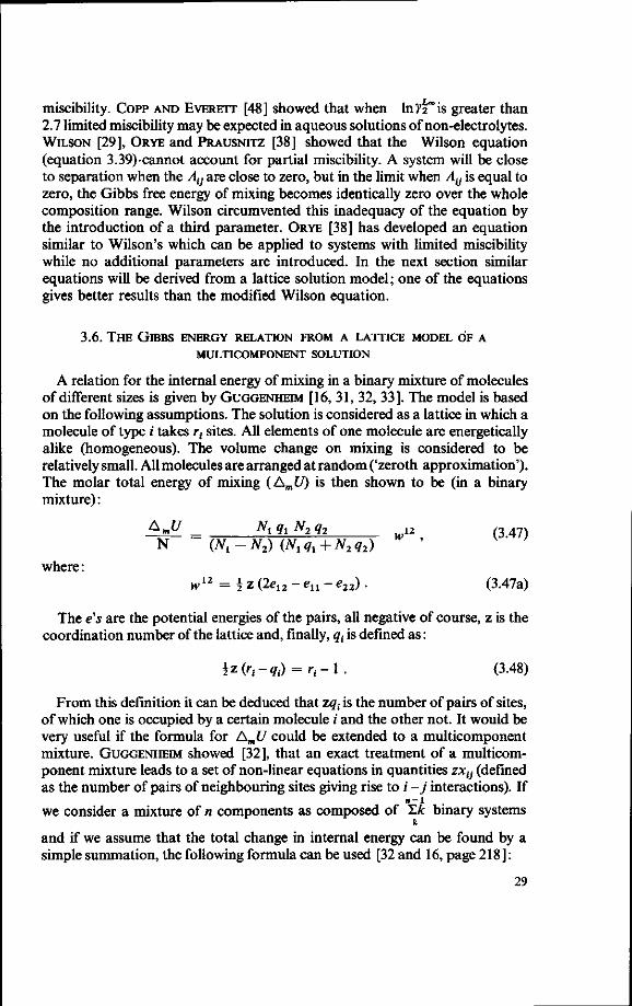
3.6. THE GIBBS ENERGY RELATION FROM A LATTICE MODEL OF A

MULTICOMPONENT SOLUTION

A relation for the internal energy of mixing in a binary mixture of molecules of different sizes is given by GUGGENHEIM [16, 31, 32, 33]. The model is based on the following assumptions. The solution is considered as a lattice in which a molecule of type / takes rt sites. All elements of one molecule are energetically alike (homogeneous). The volume change on mixing is considered to be relatively small. All molecules are arranged at random ('zeroth approximation'). The molar total energy of mixing (Am£7) is then shown to be (in a binary mixture):

where:

The e's are the potential energies of the pairs, all negative of course, z is the coordination number of the lattice and, finally, qt is defined as:

i z ( r , - 9 ( ) = r J - l . (3.48)

From this definition it can be deduced that zqt is the number of pairs of sites, of which one is occupied by a certain molecule / and the other not. It would be very useful if the formula for AmU could be extended to a multicomponent mixture. GUGGENHEIM showed [32], that an exact treatment of a multicom­ponent mixture leads to a set of non-linear equations in quantities zxl} (defined as the number of pairs of neighbouring sites giving rise to i -j interactions). If

n - l

we consider a mixture of n components as composed of l.k binary systems k

and if we assume that the total change in internal energy can be found by a simple summation, the following formula can be used [32 and 16, page 218]:

29

Amty N

Nt qt N2 q2

(Nt+NJ (Niqi + N2q2)

w12 = $ z (2e12 - en - e22).

w12, (3.47)

(3.47a)

A ^ £ NiqiNjqj (3 49) N Z*Nk (Z Nk qk)

W ' ' k k

where £ denotes summation over all distinct pairs of types of molecules. This

formula is known as the zeroth approximation, GUGGENHEIM [23]. If the re­lation between qt and rf is introduced in the expression for A m U one obtains

/

I (3.50)

As GUGGENHEIM has pointed out [16, p. 216], an immediate consequence of the assumption that the molecules are distributed at random, is that the entropy of mixing is independent of the energy of interchange between the molecules and therefore is the same as found in athermal mixtures. HILDEBRAND [30, p. 134] notes that the very existence of differences in the ii,jj and ij inter­actions must lead to preferential formation of pairs of some of these kinds. Guggenheim also treated this influence in his so called 'first approximation', which leads to the above mentioned set of non-linear equations in Xiy

As our objective is to develop equations for the excess Gibbs free energy containing two parameters to be determined experimentally, we will content ourselves with the zeroth approximation. Moreover the errors due to over­simplification of models are always one order of magnitude smaller in the Gibbs free energy than in the entropy and enthalpy, HILDEBRAND [30, p. 135 ].

GUGGENHEIM [16, p. 197] gives a formula for the entropy of mixing in a multicomponent mixture of molecules of different sizes, much like the formula originally obtained by HUGGINS [49]:

EM AmS -?H#) + ±zqjNjlnfe

L r, JVi ^

TqiMi (3.51)

Combination of formula (3.50) and (3.51) gives for the Gibbs free energy of mixing (assuming that AmFis zero):

=Zxdn (pX /

kT +

+ ?*HK]-

lH)»"+HI(--̂ +N k H)?*^ z *

HH" Nk/('LNk) + -i:NkrkK'ZNk) k Z k k

(l--)ri-LrkNkKJ:Nk) + -ri \ Z/ k k Z

(3.52)

30

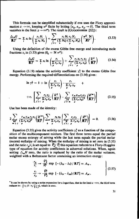
This formula can be simplified substantially if one uses the Flory approxi­mation z ->oo, keeping W1 finite by letting {eti, eti, e^-^-O). The third term vanishes in the limit z -> oo*). The result is (GUGGENHEIM [32]):

A^.= y 1 / riNi \ y nNtrjNj /w". N \ (3.53)

Using the definition of the excess Gibbs free energy and introducing mole fractions x{ in (3.53) gives (fly = N w°):

AeG _ Xim ( « \ + Z'/^i ( |^) (3-54)

ZrpXp I j (Zrp^p) \ R 7 7 \ P / i+i P

Equation (3.19) relates the activity coefficient y*{ to the excess Gibbs free energy. Performing the required-differentiations on (3.54) gives:

In yf = 1 + In

+n

\XrpxpJ I r ,

V XrPxp\*T} V (Z

+

XmfjXj /&

LJ + i P . *rPxPy

j + m p (£) (3.55)

Use has been made of the identity:

2if i'r'Xf'W)^T^TP V^TpTplRr) =0- (3J6)

" + JP * P I. fc=M P /

Equation (3.55) gives the activity coefficients yf as a function of the compo­sition of the multicomponent mixture. The first three terms equal the partial molar excess entropy of mixing while the last term equals the partial molar (excess) enthalpy of mixing. When the enthalpy of mixing is set zero in (3.55) and the ratio rp/rt is set equal to P /̂ (̂ this equation reduces to a Flory-Huggins type of equation for activity coefficients in athermal solutions. When, again setting AmH zero, the ratio is replaced by the ratio of the molar volumes, weighted with a Boltzmann factor containing an interaction energy:

• £- -> - p exp [- (Alp - kt() I RT] = Aip ,

n If — -»> - r a exp [- {Xip - XPP) I RT] = Api,

•B ' P

(3.57)

* It can be shown by using a series expansion for a logarithm, that in the limit z -xx>, the third term reduces to: £x, (\-r,/1 rx), which is zero.

31

the Wilson equation is obtained. For a binary system, when the excess entropy of mixing is set to zero (regular solutions), the classical Van Laar equations can be derived from (3.55) on introduction of parameters:

I ip — fn ' R T '

rPl = r, ̂ ,

when it is assumed that wp = up{. In this case the ratio between rp and r, is replaced by:

(3.59) /j> _ I ip

Which parameters (Ai} - or ry - type) should be chosen and which part of equation (3.55) (the entropy or enthalpy part) deleted, is mainly a question of the best representation of thermodynamically consistent experimental vapour liquid equilibrium data for as large a number of systems as possible.

The Wilson equation has been investigated very thoroughly in recent literature, PRAUSNITZ [18], NAGEL AND SINN [36], WILSON [28]; the Van Laar equation is one of the most commonly used equations. Other choices that have not been studied are the following:

(i) The total equation (3.55) with T-parameters; (ii) The total equation (3.55) with yl-parameters;*) (iii) The entropy part of (3.55) with T-parameters; (iv) The enthalpy part of (3.55) with A -parameters.

All these equations only need binary data for extension to multicomponent systems and feature a built-in temperature dependence of the activity coef­ficients. Some of them are also suitable for systems showing limited miscibility; this last property being especially attractive in non-electrolyte systems with water as a component. It will now be proved that the combination (iii) will not yield an equation able to predict phase separation in a binary system, after which the other equations will be discussed consecutively. Introduction of the T-parameters in the entropy part of (3.55) gives for the activity coefficient lnyf in a binary system:

In yh = 1 - In Ixi + -=¥- x2\ 1 , A 2 "

Xl + -=— X2 1 21

(3.60)

For the partial molar Gibbs free energy one can deduce:

* However the same relations resulting from this choice have been derived (in 1965) by R. V. OR YE [17] in a different way.

32

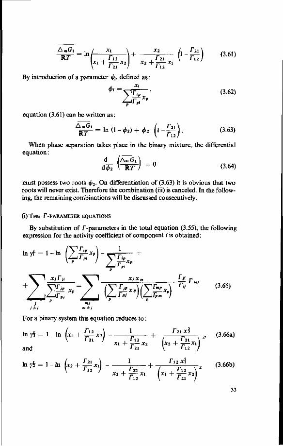
AmGi . / xi \ , xi ^/ -rM+^H'- fe) <»» Ul + 7;— -X2 / x2 + j ; — Xl \ i 21 / i 12

By introduction of a parameter (j>h defined as: 1 Xi

(3.62) / .r **

equation (3.61) can be written as:

l n ( l - 0 2 ) + </>2 ( l - ^ ) . (3-63) AmGi RT

When phase separation takes place in the binary mixture, the differential equation:

d /A .G i \ d ^ \ ~ R T 7 = ° (3-64)

must possess two roots (j)2. On differentiation of (3.63) it is obvious that two roots will never exist. Therefore the combination (iii) is canceled. In the follow­ing, the remaining combinations will be discussed consecutively.

(i) THE /"-PARAMETER EQUATIONS

By substitution of /"-parameters in the total equation (3.55), the following expression for the activity coefficient of component / is obtained:

In yf = 1 - In (Y^-x,) - = - i +

p

2 Xj fjj X 1 XjXm ^ T

j mj J+ i m+ j

For a binary system this equation reduces to:

1 , r 2 i xi In y\ = 1 - In L + ^x2) ^ — + Xl + jP "

and 1 2 X2 + jr^-Xl)

(3.66a)

In -fy = 1 - In (x2 + ^xi) L + . r "_ X l x 2 (3.66b)

*2 + -=— Xl i 12

33

The temperature dependence of /"-parameters is given by (3.58), from which other parameters (e) can be deduced according to:

Sip

Rf , rpt Epi

Kf (3.67)

Theoretically the e-parameters should be more constant with variation of temperature than the /"-parameters.

It will now be proved that for a binary system the equations are applicable to systems showing partial miscibility. For component / the partial molar Gibbs free energy (on introduction of the /"-parameters into (3.53)) can be written as:

AmGi KT

In Xl

KM + rtX2) i+

Xl

,r21 X2 + -p— Xl

I 12

( - f e ) +

+ xi r2i xi xi r2i

(3.68)

Introducing 'volume fractions' 0f as in (3.62) equation (3,68) can be written

as: AmG: KT

'-=ln (I-<i>i)-42(1- ^)+ r2l<f>i (3.69)

In FIG. 3.1 the partial molar Gibbs free energy of component 1 in the binary mixture is plotted against the volume fraction 4>i. At temperatures above the critical solubility, the curve will show monotonic behaviour, satisfying con­dition (3.44), at temperatures below the critical solubility the curve has a maxi­mum and a minimum, shown at A and B respectively. The two coexisting phases are shown as C and D'. The condition for critical mixing is that A and B coin­cide. Differentiating (3.69) with respect to 0 2 gives:

d d<£2 M = - T ^ ( ' - £ ) + ̂ r - (' 70)

The points A and B are characterised by:

d d<^2

rAmGi"|

L **" J 4>* = 0.

C,D

From (3.70) one can see this to be equivalent to:

T~4>2 in l + 1 - %)*> + 1 = 0 . (3.71)

The solution of which is:

34

FIG. 3.1. Partial molar Gibbs free energy as a function of the volume fraction $ in a binary mixture.

*,'• •"-r"^.:r"rr")[-±(-* (4r 1 2 r 2 i ) 2

r i2 (2 r i 2 r 2 1 + r 2 i - r 1 2 ) 2 I1] (3.72)

The condition of critical mixing is that the two roots coincide, giving:

2 = (VT2T- yTf^)2 (3 7 3) r21 =

Formula (3.73) can be rewritten for the critical mixing temperature Tc using (3.46):

2 s12 i /r21 Rrc,

1 (3.74) 12

Formula (3.74) was given in slightly different forms by GUGGENHEIM [16] and FLORY [50] (by the latter for the case r2 = 1).

If component 2 is present at infinite dilution in component 1 (the solvent), the following expression for the limiting values of the activity coefficient of component 2 can be deduced from (3.66b):

35

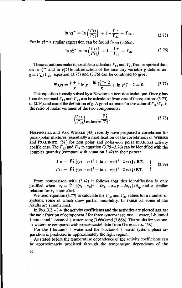
tarf- = in(£) + i -£ + r i a . (375)

For In yf ~ a similar expression can be found from (3.66a):

l n y t - = l n ( ^ i ) + l - ^ i + r 2 i . 0-76)

These equations make it possible to calculate T12 and T21 from empirical data on In yf"" and In y^TOn introduction of the auxiliary variable g defined as: g == rl2/r21, equation (3.75) and (3.76) can be combined to give:

Tig) s £ ± i l n g - l n y ^ ' 2 + In y V - 2 = 0. (3.77)

This equation is easily solved by a Newtonian iteration technique. Once g has been determined T12 and r 2 1 can be calculated from one of the equations (3.75) or (3.76) and use of the definition of g. A good estimate for the value of rn/r21 is the ratio of molar volumes of the two components:

m = £ £ (3-78) estimate KT

HELPINSTILL and VAN WINKLE [43] recently have proposed a correlation for polar-polar mixtures (essentially a modification of the correlations of WEIMER

and PRAUSNITZ [51] for non polar and polar-non polar mixtures) activity coefficients. The f12 and T2Y in equation (3.75-3.76) can be identified with the complex quantity (compare with equation 3.42) in their paper:

T 2 1= P5[(<r,-(72)2+(ffn-ff22)2-2ffi2]/Rr, )

r2l= ^H(ffl-ff2)2 + (ff11-ff22)2-2(7l2]/Rr. )

From comparison with (3.42) it follows that this identification is only justified when r t = 9[ {(o^ -cr2)2 + (<ru -a22)

2 -2a12}/uip and a similar relation for r2 is satisfied.

We used equation (3.77) to calculate the T12 and T21 values for a number of systems, some of which show partial miscibility. In TABLE 3.1 some of the results are summarised.

In FIG. 3.2.-3.4. the activity coefficients and the activities are plotted against the mole fraction of component 1 for three systems: acetone + water, 1 -butanol + water and 1-octanol + water using (3.66a) and (3.66b). The results for acetone -> water are compared with experimental data from OTHMER C.S. [58].

For the 1-butanol + water and the 1-octanol + water system, phase se­paration is predicted in approximately the right region.

As stated before the temperature dependence of the activity coefficients can be approximately predicted through the temperature dependence of the

36

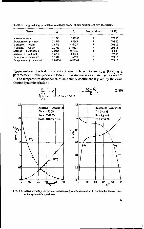
TABLE 3.1. rl2 and r2 , parameters calculated from infinite dilution activity coefficients.

System ra r2l No Iterations T(K)

acetone + water 2-heptanone + water 1-butanol + water 1-octanol + water acetone + heptanon-2 acetone + 1-octanol 1-butanol + 1-octanol 2-heptanone + 1-octanol

1.5745 2.1590 1.6545 2.2763 2.0025 3.6702 3.5548 1.80256

2.52285 9.8669 4.6425

11.6137 0.7036 0.8224 1.6639 0.83549

8 7 7 7 6 6 6 6

373.15 298.15 298.15 298.15 350.0 373.15 373.15 373.15

/^-parameters. To test this ability it was preferred to use etj ~ RTTy as a parameters. For the systems in TABLE 3.1 a-values were calculated, see TABLE 3.2.

The temperature dependence of an activity coefficient is given by the exact thermodynamic relation:

i\M $

m-Hi (3.80)

3.0

25

£ 2 0

1.5

1.0

06

\ In Y,

Acetone (1).Water (2) r« = 1.57-45 TJI = 2.52285

Data: (

X^

Dthmei

/ I n

s ^

• c.s.

»i

1.2

1.0

Q8

Q6

04

Q2

/ '

Acetone(1)-Water<2) T= 373.15 Ii2 = 1.5745 m = 2. 5228

v*

0.2 0.4 06 0.8 10 Q2 0.4 06 08 IfJ

FIG. 3.2. Activity coefficients ($) and activities (m) as a function of mole fraction for the acetone-water system (r-equations).

37

TABLE 3.2. The energy parameters etl and e21 for some systems.

System Hi cal/mole

«21

cal/mole

acetone + water 2-heptanone + water 1-butanol + water 1-octanol + water acetone + 2-heptanone acetone + 1-octanol 1-butanol + 1-octanol 2-heptanone + 1-octanol

1167.56 1279.19 980.29

1348.65 1392.76 2721.53 2635.96 1336.64

1870.75 5846.01 2750.63 6880.91 498.34 609.79

1233.88 619.54

where H? is the enthalpy of component i in the standard state. Differentiating (3.65) in .this way one obtains:

4) In yh

P.xj • 2 2? i P

**•R Z_J(2^

m, j P m+j

XjXm

R !LX\ / V £SjeF\ R

50

£ 4 0

30

Z0

1.0

\ tn

1.Butanol(1)-Wat«r(2)

n i = 1.6545

ri i = 4.6425

A

lnvL

10

08

06

04

02

; \ f \

i

}

1 .

T

\ \ " • * •

Butan

= 298

1 s

1

ol(1)-W

•K

V X

*

ater(2)

/

\

\

02 04 06 08 10 0 02 04 06 08 10 X, =0.025 ! , , O.S«0 X,

FIG. 3.3. Activity coefficients (-ft) and activities (at) as a function of mole fraction for the 1-butanol-water system (/"-equations).

38

120

1Q0

>• ao

c

?-60

4.U

20

°C

\

System

1-OctanoK1)+Water(2) _ /

\ l " Y i

) Q 2 0

1 12 = Z.Z763

Tj, = 11.6137 T = 298°K

4 0

. In

6 0 ^

v i ~

8 1. D

4

2

10'

i 6

(0 4

«o 2

10°

6

2

10"'

6

2

iff2

c

f\

\

sy stem 1-0ctanot(1)+Water(2>

\ « l

*>*' —

V

) 02 0.

—--!

i 0

\ N

.,—

6

^. "

OB 1.G

-*• Xl Xl

FIG. 3.4. Activity coefficients (•fi) and activities (at) as a function of mole fraction for the 1-octanol-water system (T-equations).

For a binary system this differential becomes (in the limit xx ->• 0) for the activity coefficient of component 2:

dlny*-;

'(kr)

[ffl-H^oo (3.82)

P, x

When e12 (in other words - [//J -.rY1]°°) is positive, heat is taken up on mixing the pure constituents 1 and 2, the value of the activity coefficient then falls with rising temperature. Equation (3.82) can only be integrated directly when the parameter £ is constant for different temperatures. The molar heat of solution of components in infinite dilution has been determined experimentally for a number of alcohols in water. It turns out that [//J - Hi ] "/R is roughly a linear function of (±), see FIG. 3.5 for experimental data on methanol-water. A fit of isobaric vapour liquid equilibrium data on the system methanol (1) + water (2) [UCHIDA and KATO, 52] to the total pressure of the system, gives the following results for the T-equations:

39

0.6021 2.0429

442.194 cal/gmol (for T 765.917 cal/gmol

rl2

e12 = 442.194 cal/gmol (for T .= 369.55 K) £ 21

RMS - error = 0.3616% (in total pressure)

From these fitting data a value for - [H\ - Ht ] °° /R of + 388 °K is calculated, which seems to be unreasonable (see FIG. 3.5); the temperature dependence is by no means approximated. The T-equations turn out to be useful for systems snowing partial miscibility, the built-in temperature dependence however is very poor.

+800

FIG. 3.5. Partial molar heat of mixing at infinite dilution as a function of reciprocal temperature for the methanol-water system compared with predictions of f- and 4-equations.

40

(ii) THE /1-PARAMETER EQUATIONS.

Introduction of the /1-parameters (Wilson parameters) is possible when the energy utj is related to these parameters. This is possible from comparison of the definition of these parameters with equation (3.47a). For fiy it can be written:

Utj = N wi} = i z (2 en N - ea N - ejj N) (3.83)

From the Wilson equations it is clear that Xtj, XH and kn are proportional to the interaction energies ey, eit and en. Hence:

I z N e y - Xu (3.84) therefore: g^ Ifa-fa-Xg

RT~ RT (3-85)

The right hand side of (3.85) is easily shown to be given by the logarithm of the product (yly • A}i). It would therefore be tempting to replace r-utJ by:

n uu = - n R J In (yt„ ̂ ) (3.86)

This equation is far from exact, because the differences in interaction energies between ij, ii and yy-pairs, we anticipate, in essence lead to other equations for the enthalpy of mixing than those used. Accepting (3.86) leads to the equation for the excess Gibbs free energy obtained from (3.54):

%r = -£Xi{ZAijXj) - r ,Z(i**s , ) -fr <*"*«>• « J l " (3.87)

The physical meaning of r{ is that it represents the number of sites in a quasi-cristalline lattice model, which will be occupied by the molecules of type i. If one considers a molecule i in an environment of a mixture of molecules / and

j , the structure of the lattice should be a function of the relative amounts of/' and j molecules. In other words one can expect that the average distance between two sites is a function of the composition of the liquid; a molecule /' surrounded by moleculesy which are half as big would occupy two sites, but when the con­centration of molecules /' increases to pure /' a transition to an r, value of unity would be logical. Postulating that the 'dimension' of a molecule / is directly proportional to the molar volume (Vf), an approximate expression for ri would be the ratio between the molar volume of the molecule /' divided by a 'mean' molar volume (V%) of the solution:

ri~7\- z VlPxP ~V^T- ' TA~TP '

(3'88)

P Z-i~V*iXp p

The 'mean' molar volume is constructed by weighting the molar volumes of all the constituents with their mole fractions. The definition of rt predicts in a

41

dilute binary system of i inj a value for rt close to the ratio of molar volumes {9\lVj), while for a more concentrated solution the value approaches unity.

The last transition in (3.88) is logical in view of the definition of the Wilson parameters (3.37) and the argument that the interaction energies between the molecules may influence the lattice dimensions too. By introduction (3.88) into (3.87) one obtains:

^ - - Ss-In (£.!•• x l X I XiXjlnjAjjAjj) ( 3 8 9 )

J + i P P

An expression for the activity coefficients could be derived straight from (3.55) using also (3.88) to eliminate the remaining rt, however the undesirable situation would then arise that the activity coefficient equation does not match with the excess Gibbs free energy equation (3.89) as prescribed by equation (3.19). Therefore a better expression can be derived by application of the operation (3.18) to the Gibbs free energy relation (3.89).

The result is:

l n t f= 1-In (L , ! «* , ) -> \*UA "A + V T X„Ami "1

Z-j|(£/lmpXp)J (3.90) xj In (Atj Aji) V^ X]Xm\n(AijAji) V xjlnjAijAji) y

jLi(.?LAipxP){?.AipxP) « Z J , I

[J.Aipxp) CLAjPxP) "f ' Z_J (X,AjpxP) CZAmpXp) P P m,j p p

m * j + i

where:

^ M 1 - ! ^ - ! ^ } (391) \ p p '

4 m S l - - 4 j ! — - A" . (3.92) Li sijp Xp 2d A. mp Xp

P

The last summation in (3.90) only arises in multicomponent systems. For a binary system the activity coefficient of component / is:

h y { = (In yfi x2\n(A12A2i) H ^ l ™ Wibon {xi + An X2) (X2 + A2lXl)

{ 1 + Xl (l - _ i -£%—)\ (3.93a) ( \ X1+/I12JC2 X2 + A2lXl)\ '

and for component 2:

In yS = (In yi) ^ In (/t12^2i) 7 K y ' w i l *>» (Xl + ill 2 x2) (X2 + A21X1)

li + x»(i - 1 £r—)\ (193b)

[ \ X2 + /I21X1 Xi + A12X2J) 42

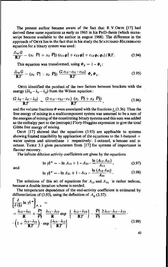
The present author became aware of the fact that R.V.ORYE [17] had derived these same equations as early as 1965 in his PHD-thesis (which manu­script became available to the author in august 1968). The difference in the approach of ORYE lies in the fact that in his study the SCATCHARD-HILDEBRAND equation for a binary system was used:

A m G = (Xl V\ + X2 9h) (C110? + C22&1 + C1201 $2 ) /R7 \ (3.94) RT

This equation was transformed, using # 2 = 1 - 01:

^ = (*! n+X2 n ( 2 c i 2R

c ^ " C 2 2 ) *i*2. (395)

ORYE identified the product of the two factors between brackets with the energy (2Xtj - kti - Aj7) from the Wilson equation:

(2Xij-Xu-Xjj) (2C12-C22-Cu) (Xl ?\ + x2 PS") (3.96) RT RT

and the volume fractions $ were associated with the fractions £. (3.36). Then the free energy of mixing in a multicomponent system was assumed to be a sum of the energies of mixing of the constituting binary systems and this sum was added as the enthalpy part to the (entropic) Flory-Huggins expression to give the total Gibbs free energy of mixing.

ORYE [17] showed that the equations (3.93) are applicable to systems showing limited miscibility by application of the equations to the 1-butanol + water system and nitroethane + respectively: 1-octanol, n-hexane and n-octane. TABLE 3.3 gives parameters from [17] for systems of importance in flavour recovery.

The infinite dilution activity coefficients are given by the equations

In yk~ = - In Al2 + 1 - Atl - ln^/A^ , (3.97) , Al2

lnyr = - l n^ 1 + l - ^ - l n ( y l ! 2 / l 2 l ) . 0-98)

The solutions of this set of equations for A12 and A21 is rather tedious, because a double iteration scheme is needed.

The temperature dependence of the end-activity coefficient is estimated by differentiation of (3.93), using the definition of AtJ (3.37):

[4*"*i--An V\ A12-A22 I A12-A22) V\ 2Ai2-An-A22 , - , f A12-A22) V\

(3.99) R Vh R

( , . Ai2-An\ fAi2—An]

1 + -R r - j e x p ( -R3- - ) 43

TABLE 3.3. Parameters for the A-equations for some systems, Orye [17].

Nc

1

2

3

4 5

6

7

8

9

10

(. System (1) + (2)

acetone + methanol (100 °C)

methanol + water (100 °C)

acetone + water (100°C)

acetone + methanol methanol + water

(1 atm) (1 atm)

acetone + water (1 atm)

acetone + methylisobu-tyl ketone (1 atm)

methylacetate + methanol (50 ° Q

acetone + methylacetate (50 °C)

water + Rmtanol (1.009 atm)

ft Vi (cm3/mole)

•

82.995

44.874

82.995

42.109 78.470

77.652

84.345

81.361

76.826

19.014

44.874

18.844

18.844

18.408 42.067

18.338

138.022

41.247

81.361

99.380

Xn— An (cal/mole)

-696.

-112.71

-533.42

-226.79 -291.33

-484.86

610.57

-335.80

245.66

1077.38

A12-22 (cal/mole)

813.07

344.50

1102.29

464.69 460.14

1026.97

-543.62

629.66

-188.99

-404.58

Rotation of the index 1 -*• 2 -*• 1 gives an analogous expression for the temperature dependence of In y\°°. In FIG. 3.5 some lines are drawn, calculated with these equations for the alcohol methanol in water. Although the numerical values predicted for the heat of mixing at infinite dilution are wrong, the trends in the curves are approximately correct. For moderate temperature differences the temperature dependence of the activity coefficients in the example can therefore be predicted with more accuracy than any other 'two parameter' equation could do.

(iv) ENTHALPIC /1-PARAMETER EQUATIONS

When the entropy part of (3.55) is deleted (regular solutions concept) the equations for the activity coefficients are the same as derived in the preceeding section except that the 'Wilson part' of the equations is absent:

In A = _ V xj In (AjjAji) y XjXmln(AmjAjm)nlmji

my' Zj(S/l ip^)(Z^Pxp)l^J "•" AJ {XAjfXjiZAmfX,) '

I P P mj p m+i, + i (3.100)

with n°u and n\im again given by (3.91) and (3.92). These equations predict for a binary system in which one of the components is present at infinite dilution:

Xnyk = MT~ ' < 1 ^ 2 " " 1 ) - (3.101)

44

These equations are easily solved with a Newtonian iteration scheme, the value for A 21 is the root of the equation:

'»fe£] -«" (A21) = 2 In (/I21) + /I21 In y i " + In ^ p = 0. (3.102)

The fact that the set (3.99) is solved easily is a distinct advantage of these equations over the /1-equations, as the activity coefficients at infinite dilution are often known (see section 3.4), or can be estimated from correlations. In APPENDIX 3.A a FORTRAN-programme (ENTLAM) developed to calculate /1-values from end coefficients is given. In TABLE 3.4 some results are given for methanol, ethanol and 1-butanol.

TABLE 3.4. Estimated yi-parameters for Enthalpic /1-equations from activity coefficients at infinite dilution (ENTLAM-programme).

System Parameters Temp. . iterations

methanol/water (1.0 arm) ethanol/water (1.0 atm) 1-butanol/water (1.0 atm)

The dependence of infinite dilution activity coefficients on the temperature is for the Enthalpic /1-equations:

A* 0.5990 0.4832 0.3049

*u 0.9944 0.9280 1.0054

^i2~^n

-257.553 -364.712 -344.979

*12 *22

638.017 952.309

1220.001

(°K) 369.55 368.65 372.65

6 6 6

Mr1"*!: 2A12-A11-A22 _Pt / | . A12—Aii

R 9h \ RT

exp { ^ } . (3.103)

For methanol-water the results of this equation are also plotted in FIG. 3.5, the picture is approximately the same as for the /l-equations The Enthalpic /1-equations are, in fact somewhat closer to the actual numerical values than the /1-equations.

In the next section the equation will be discussed more extensively.

3.7. COMPARISON OF THE DERIVED ACTIVITY COEFFICIENT EQUATIONS

The equations derived in section (3.6) were tested for a number of binary systems, all of which contained water as one of the components. Moreover all systems selected were isobaric to test the built-in temperature dependence most effectively.

The fitting procedure used was that proposed by PRAUSNITZ ET AL. [18]. The total pressure of the system is fitted to the specified pressure of the system by adjusting the two parameters in the activity coefficient equation (HVYFT-

45

programme). *). Prausnitz c.s. used the SHARE-programme EZNOLSQ [18], a non-linear multiple-regression subroutine which adjusts the parameters of a function being fitted to data in such a manner as to yield a least squares fit. This programme was not available, therefore a 'steepest descent' programme was used in this study.

The outlines of the method used were given by MARQUARDT (1959) [53]. A FORTRAN-programme was written for the special case of two fitting parameters. The programme builds up a surface in the three dimensional space formed by the sum of squares of deviations axis ('S') and the two parameter axes (Pt, P2). Two components of the gradient vector to the surface at a certain location in the space were determined and the parameters P1 and P2 were adjusted following the direction of the projection of the gradient vector on the (Pu P2)-plane. The step size is fixed initially but is corrected by the programme following the metric of the surface. Protection against overshoot of the minimum location was built in. The programme is very insensitive for the initial guess of the values of the parameters. It required five calculations of 'Z'-values in a grid (. : .)for the estimation of the direction of the gradient vector projections, while in quadratic models at least seven points are needed. The criterion to finish the calculations was that the absolute value of the relative difference between two successive estimates of the sum of squares of percent deviations had to become

TABLE 3.5. Literature data for the systems selected to test activity coefficient/composition equa­tions.

(all isobaric at 1.0 atm.) methanol - water UCHIDA & KATO [52 ](1934) ethanol - water CAREY & LEWIS, NOYES & WARFLE [54,55] (1932) 1-butanol - water STOCKHARDT & HULL [56] (1931) s-butanol - water ALSYBEEVA & BELOUSOV [47] (1964) acetone - water OTHMER c.s. [58] (1952) butanone - water OTHMER, CHUDGAR & LEVY [58] (1952) methylacetate - water MARSHALL N. [59] (1906) furfural - water Int. Crit. Tables [60] (1928)

smaller than 10"5:

-n+ 1 ^ Mr5.

A somewhat better resolution for very accurate results is obtained from a criterion, based on differences between the parameter values (this criterion was used by PRAUSNITZ), however a relative large amount of extra computer time will then be needed. For the purpose of comparing the abilities of the different equations the accuracy of the method used seemed to be satisfactory.

The time needed for calculation of one system varied rather strongly among

* The programme is available in ref. [18], slight modifications were applied, only to make the programme suitable to an other minimising procedure.

46

TABLE 3.6. Fitting results for Wilson-equations for some systems.

System

methanol/water 1.0 atm.

ethanol/water 1.0 atm.

acetone/water 1.0 atm.

Parameters ^12-^.11

(cal/mole)

198.1125

380.3149

469.020

Al2—A22

(cal/mole)

472.3676

910.6148

1489.07

Molar volumes

vt (cm3/mole)

42.109

63.977

81.420

(cm3/mole)

18.792

18.779

18.675

T (°K)

369.55

368.65

361.00

Error in p total*)

0.3612

1.1578

2.6999

*) See table 3-10 foot note

TABLE 3.7. Fitting results of T-equations for some systems.

System

methanol/water 1.0 atm.

ethanol/water 1.0 atm.

1-butanol/water 1.0 atm.

s-butanol/water 1.0 atm.

acetone/water 1.0 atm.

butanone/water 1.0 atm.

methylacetate/ water 1.0 atm.

furfural/water 1.0 atm.

r,2

0.6021

0.9875

1.5696

1.5093

1.4392

1.8041

1.6971

1.7366

Parameters

r2l

1.0429

1.9225

4.6182

4.2917

2.5208

3.7793

3.1399

5.4891

£12

(cal/mole)

442.194

723.459

1162.336

1093.13

1032.47

1282.593

1214.279

1282.7625

«21

(cal/mole)

765.917

1408.405

3419.983

3108.21

1808.37

2686.815

2246.5855

4054.6301

T fK)

369.55

368.65

372.65

364.45

361.00

361.00

360.05

371.710

Error in p total*)

(%)

0.3616

0.6503

4.0834

1.7815

5.2401

5.5858

6.3476

24.1892

*) See table 3-10 foot note

TABLE 3.8 Fitting results for Van Laar equations for some systems

System

methanol/water 1.0 atm. ethanol/water 1.0 atm. 1-butanol/water 1.0 atm. s-butanol/water 1.0 atm. acetone/water 1.0 atm. butanone/water 1.0 atm. methylacetate/water, 1.0 atm. furfural/water 1.0 atm.

*) See table 3-10 foot note

Parameters

A,2

0.8649 1.6601 3.8772 3.5447 2.3880 3.5045 3.0565 4.6895

A21

0.5210 0.8643 1.1759 1.1387 1.4555 1.6525 1.8050 1.1008

Error in p total*)

<%)

0.3521 0.7246 3.3491 1.4795 4.4151 5.1996 5.5212

27.5862

47

TABLE 3.9. Fitting results for Enthalpic A-equations for some systems.

System Parameters

(cal/mole) (cal/mole) (cm3/mole) (cm3/mole)

Molar volumes ~PF r

CK)

Error in /> total*)

(%)

methanol/water 1.0 atm.

ethanol/water 1.0 atm.

1-butanol/water 1.0 atm.

s-butanol/water 1.0 atm

actone/water 1.0 atm.

butanone/water 1.0 atm.

methylacetate/ water 1.0 atm.

furfural/water 1.0 atm.

-208.7681

-325.7964

-357.8748

-279.327

-436.468

-396.248

-419.1093

-202.367

571.3078

897.1059

1229.9084

1098.612

1185.436

1307.900

1290.6923

1158.676

44.548

63.977

98.366

85.668

81.420

89.533

87.373

82.899

18.792

18.779

18.837

18.721

18.675

18 633

K.663

18.823

369.55

368.65

372.65

364.45

361.00

361.00

329.63

371.71

0.3473

0.6506

4.1245

1.6216

3.2695

4.1933

3.4580

23.0276

See table 3-10 foot note

TABLE 3.10. Fitting results for A-equations for some systems.

System

methanol/water 1.0 atm.

ethanol/water 1.0 atm.

1-butanol/water 1.0 atm.

s-butanol/water 1.0 atm.

acetone/water 1.0 atm.

butanone/water 1.0 atm.

methylacetate/ water 1.0 atm.

furfural/water 1.0 atm.

Parameters A12-A11

(cal/mole)

-211.440

-348.018

-369.779

-279.327

^79.035

-435.140

-419.1093

-231.3797

A12—A22

(cal/mole)

450.860

747.2929

1043.374

921.84

1023.049

1122.348

1290.692

970.618

Molar volumes Vk

(cm3/mole)

44.548

63.977

98.366

85.688

81.420

89.533

87.373

82.899

n (cm3/mole)

18.791

18.779

18.837

18.721

18.675

18.633

18.633

18.823

T CK)

369.55

368.65

372.65

364.45

361.00

357.75

329.63

371.71

Error in p total*)

<%)

0.3479

0.7323

4.4161

1.7331

4.0037

4.9331

4.4630

23.2258

*) The error is defined as

AP \ 1 (PcaU.t-Pexp.l.

i = 1 r„u, i

V (AP)

•, with N the number of measurements and AP: tf-2

1002

48

different types of equations, but was of course also dependent on the efficiency of the initial guess of the values of (P,) and (P2) and the number of measure­ments. On the average about 1.5 hours computer time of a IBM 1130 digital computer was needed for one system. The complete /1-equation and the Wilson equations however required about 2 hours in general.

The systems selected are given in TABLE 3.5. The results of the calculations are summmarised in TABLE 3.6-3.10. General

trends are that the F-equations give a poor result when compared with the Van Laar equations. A remarkable result is that the Enthalpic /4-equation shows a lower error for six out of the eight systems than the Van Laar equations. Therefore the use of the Enthalpic /4-equations is recommended for calculations on systems where phase separation occurs. Moreover an easy estimate of the parameters can be obtained from infinite dilution activity coefficient data (section 3.6) for this equation, while the smaller amount of computer time needed for calculations with the HVYFTW-programme is also notable. The Wilson equation gives better results than the other equations for acetone water. For methanol-water and ethanol-water the results are less accurate than the Van Laar equations.

49

4. CALCULATIONAL PROCEDURES FOR MULTICOMPONENT DISTILLATIONS

4.1. PLATE TO PLATE CALCULATIONS

Multicomponent distillation has been, and still is, an item which invoked many research projects in the petro-chemical industries and the computational procedures were largely developed in this industry. It is beyond the scope of this study to present an extensive review of all the different techniques used for the calculations.

The calculation method used in the present study is the THIELE-GEDDES procedure [61, 8 J"). In this procedure the temperature of each plate is selected as an independent variable. First a trial temperature distribution over the plates is introduced and in successive trial and error calculations the temperatures are corrected until the material balances are satisfied.

As pointed out in section 1 already, the distillation columns used for volatile aroma recovery are 'conventional' columns. For the model calculations it was assumed that a single feed is introduced and two streams are withdrawn: viz.

;the top and the bottom products. It is assumed that a total condensor is used, hence all the vapor leaving the top plate is condensed completely to the liquid state. A part of this liquid is withdrawn, as distillate, the rest is returned as reflux. The molar flow rate of the distillate is denoted by D. The plates are numbered consecutively from the top to the bottom of the column. The reboiler is given the number N+ 1, the bottom plate the number N, the feed plate number/, the condenser the number zero. In FIG. 4.1 the notation is explained further.

For a conventional column the material balances and equilibrium relations (yt — KtXi) are expressed in the following set of equations:

-FT—— = Ae,t + 1 (condenser balance), i=\,n; (4.1) UXDi

+ 1, i=\,n; (4.3) Y/Xn = » (Vf-iXr-Li\ DXDI * U V Dxm J

"(w^) + u '-'•""): (44)

^ S r I = s ' ' ( f e ) + '• /+ '<7<*. ' - i .»; (4.5)

WxWi

* In essence a simplified method is used, in which enthalpy balances are omitted. T h e bar indicates that introduction of a stream is accounted for. The symbol q is used to indicate the thermal condition of the stream to the feed plate in the usual way: Vt — L + D-(\-q)F and Lf.1=L + qF.

50

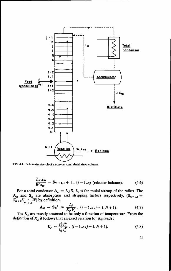
Feed (condition q)

j=1 2 3 4 5 6

i

<

F

xFi

f - 2 f - 1

t * 1 f + 2

N-6 N-5 N-4 N-3 N-2 N-1

N

N + 1

Total condenser

I Accumulator

I i

i I

1 1 —

D.XDi

Distillate

•*• Residue

FIG. 4.1. Schematic sketch of a conventional distillation column.

Wxwl SN +i,,- + 1, ( /=! ,«) (reboiler balance). (4.6)

For a total condenser Aci = LJD, L„ is the molal streani of the reflux. The An and Sjf are absorption and stripping factors respectively, (Sjy+1(i = VN+lK I W) by definition.

-i _ Lj N+l,i

Aji = &ji — Kji V, , (i=l,n;j=l,N+l). (4.7) — j* • j

The Kfi are mostly assumed to be only a function of temperature. From the definition of A}, it follows that an exact relation for Kjt reads:

ybfl Kji = $W> (i=l,n;j=l,N+l). ''ijJij

(4.8)

51

The use of relation (4.8) in an actual distillation programme is perfectly possible with the calculation schemes of PRAUSNITZ C.S., [18], however the incorporation of this scheme will not always be feasible because of the re­latively large amount of computer time needed for such calculations and the fact that these calculations form the most frequently repeated part of the computations in successive iterative solution of the material balance equa­tions. A rather modest error will be introduced if one replaces (4.8) by:

Kj, = ?¥±,i=l,n,j=l,N+l*), (4.9) i tot

which means that vapour is assumed to be a perfect gas mixture. From this equation it follows that K}i is a function of temperature and composition of the liquid on a plate. The activity coefficient yfj can of course be calculated using one of the equations reviewed in section 3.3 or section 3.6. Even this means a considerable extra consumption of computer time. In the distillation of the very dilute solutions commonly encountered in fruit juice essence recovery, it would be possible to use a more simple expression for KJt at a certain tempera­ture when the activity coefficient y$ remains constant over the concentration ranges present in the distillation column. Thus (4.9) could be replaced by:

Kjl = y-^± i + w; Kfw = | i ; j= l,N+ 1 (4.10) rtot "tot

The index w denotes water as a component. In the calculations Van Laar equations were used in conjunction with equation (4.9), to check whether further simplifications (equation 4.10) could be justified for practical situations (section 4.2).

Another assumption in the computations is that of constant molal overflow, which seems to be justified for dilute solutions, in which no impressive enthalpy content changes will occur.

In the Thiele-Geddes method the assumed initial temperature profile was taken linear, between the boiling point of the least volatile and that of the most volatile component. Starting at the condenser equations (4.1)-(4.4) are used down to the feed plate; starting at the reboiler (4.6) - (4.4) are used up to the feed plate. A complication in the calculations is the fact that enormous differ­ences in volatilities between components are anticipated. Therefore com­ponents may leave the column either only in the distillate ('separated light' components), or in the waste product ('separated heavy' components). For both types of components, which must be detected first in the calculations by use of (4.1)-(4.6), the balance equations (4.1) - (4.6) need modifications which will be discussed. Such components can be detected by means of the value of the ratio (Wxwl/DxDi), if this ratio becomes very small for a certain component i on some plate it is called separated light component, when the ratio becomes very large the component i is called a separated heavy component.

* However, see section 4.2, possibly an improvement can be achieved by use of (4.20) replacing (4.9). The activity coefficients in this chapter are not adjusted to zero pressure.

i

52

HOLLAND [8, p. 154 etc.] suggests a computational procedure for such com­ponents. In the calculations from the top plate downward and from the reboiler upward separated heavies and lights are detected respectively. For these separated components the computations with (4.1) - (4.6) are discarded. Concentrations of heavy separated components in the top section are computed using a mass balance around the bottom of the column and some plate in the top section:

Lj-i Xj-i,t „ (LjXj{\ . FXFi , . . . r . . . /A i%\

Wxwi = Sji [WxVj +1-fVx^'l<J<f-hl=l'n- ( 4 H )

And, in an analogeous way, the calculations for a separated light component in the bottom section are performed using a balance around condenser and some plate in the bottom section:

£^-=A (Vj-> yj~1-i) +1 - ^ ; / + 1 *j<N+ 1, i= \,n. (4.12) DXDI j-vi\ D xm ) DxDt

Once a composition distribution is computed, the convential calculational procedure is to estimate a better composition distribution in vapour and liquid phase from the fractions calculated with the plate-to-plate procedure. These corrected mole fractions are then used to estimate a new temperature profile using either a bubble temperature or a dew temperature calculation for each plate.

A more rapid convergence is however achieved with the so-called S-method of convergence, HOLLAND [8, p. 82 etc. ]. In this method xDi and xWi are cor­rected before plate compositions are calculated, in such a way that the cor­rected set of xDi's and xw/s satisfies the conditions:

i(DxDi) co, (4.13) i = 1

FXFI = {DxDi)co + (Wxwi)co; i = \,n. (4.14)

( )„ indicates the corrected value of a variable, ( )ca will denote the calculated value. This correction is expressed in a factor defined by:

fc).= H^L (415)

The value of 9 is found as the solution of the '^-equation' which is obtained by combining (4.15) and (4.14):

ii

* M = X , . Fn

XFwxm-D=°- <4i6> iTi 1 + 3

DXDI

The root 9 can be found as a positive number satisfying (4.16) and by use of Newton's iteration technique. Once (xWi)co are calculated:

53

(DXDOCO = / u / . ; i=l=H,L, 1 + 5 &

\ DXDi/co

(Wxwi)co = 9 { ^ m \ • {DxmU; i+ H,L, \ JJ Xm J ca

Wxm = FXFI

DXDI = FXFI

i=H, i = L.

(4.17)

The compositions in vapour and liquid phase can be computed using the following formulae:

(^A (DXDi)co yji = ^ \OXDtU . {.+ H)^ ( 4 _ l g A )

2 (***) i= l \DXDilc

( Lxjj \ \WxWiJa

(DXDi)co

(WxWi)Cl

i= i \Wxm),

; ( i f L ) . (4.18B)

Wxmh Wi lea

The numerator of (4.18 A) is indeterminate for a separated heavy component, therefore the following formula must be used for such a component:

yji = — , {Vyjl)ca Ai = H). (4.18C)

9 S ( ^ ) (DXDi)co

Similarly for a separated light component:

Xji = _ ^ i ^ f ? . ( / = L) . ( 4 . 1 8 D )

fr{ \ Wxm)c (lVxm)c,

Equations (4.18A) - (4.18D) result in corrected mole fractions on each plate in the vapour and liquid phase. However these compositions do not add up to unity until the right temperature profile is attained. A better approximation to the actual temperature distribution is obtained by a bubble temperature or a dew temperature calculation. A bubble point temperature calculation is in general to be preferred. The (positive) value for T} that satisfies:

0 (7}) ^ S Kj,(Tj; xn, i= l ,n) */, - 1 = 0 ; ( / = hN+ 1) , (4.19) i = 1

54

is the bubble temperature on plate j associated with the corrected mole fractions. 7} is determined for each plate and all the calculations are repeated until convergence is obtained, which means that all uncorrected vapour- and liquid phase mole fractions on each tray add up to unity.

4.2. RESULTS OF DISTILLATION CALCULATIONS (THIELE-GEDDES)

The calculation scheme presented in the preceeding section was programmed (APPENDIX 4.A), this scheme will be indicated with: MCDTG. The programme was developed for three purposes:

(i) To obtain information about concentration distributions and activity coefficient distributions in typical flavour distillation circumstances.

(ii) To provide data on the effects of variations in fundamental process variables as reflux ratio, moles of feed/moles of distillate ratio, number of plates, feed plate location and thermal condition of the feed when in each case all other parameters are kept constant.

(iii) To be used as a reference for a second distillation programme (MCDTG-

EFF) in which the Murphree plate efficiencies are included in the calculations. The aspects (i) and (ii) will be discussed in this section, the third in section 4.4. Two mixtures were selected for the calculations. The first was a 5 component

mixture (I) of ethylacetate, ethanol, 1-butanol, methylanthranilate and water (the sequence of the components was conventionally the direction of in­creasing critical temperature, see APPENDIX 5.C). This mixture has a vague resemblance to Concord grape juice, at least in the 'distribution' of physical properties amongst the components. The second mixture (II) consisted of methanol, 2-heptanone, 1-octanol and water. First the results with mixture (I) will be discussed. The feed composition of the mixture is given in TABLE 4.1.

TABLE 4.1. Composition of feed, mixture I.

Component (0

1. methylacetate 2. ethanol 3. 1-butanol 4. methylanthranilate (ortho) 5. water

XF,

0.1635 x 10 "6

0.4340 x 10 "* 0.7291 x 10 - ' 0.2370 x 10 "6

0.9999562

The location of the freed tray was varied keeping other process variables stant. The specification of the constant factors is given in TABLE 4.2.

TABLE 4.2. Specification of distillation calculations, mixture I.

F D q R (L/V) N P

= 2.600 (moles per = 0.008 (moles per = 0 (saturated = 0.997 = 10 (total number = 1.0

sec) sec) vapour feed)

og plates) (ata)

55

The reboilratio(V/F) is 2.56% in this case. Binary interaction parameters were obtained from data in literature, such

as: PDD-correlations, GARNER, ELLIS and PEARCE [62] (ethylacetate/water), ROGER and TURKOT [4] (methylanthranilate/water). Vapour pressures were calculated using equation (4C-1) in APPENDIX 5.C. with the appropriate con­stants (for ethanol, 1-butanol and water see PRAUSNITZ C.S. [18]).

In FIG 4.2 the composition distributions for methylanthranilate over the column are given for various locations of the feed plate. One sees that for a column of 10 plates the optimum location of the feed tray is the seventh. When more than seven plates are used in the top section a 'pinch' appears. The con­centration of methylanthranilate in the overhead stream is 0.5311 x 10" 4 and in the bottoms 0.7116 x 10"7. Thus a recovery of 68.9% of the methylanthrani­late is achieved. When the feed plate is the seventh plate of the column, the distribution of compositions (xJ(, yJt), the activity coefficients (y^) and equi­librium constants are those given in TABLE 4.3.a.

1

• u - 2 01 .o E 2 3 «

/

/ //

/

l\

I I I

F

II

= r

2,

3,

/,

-6

>7

Legenda : Mixture I

Methylanthranilate distri­bution Variable teed plate

l O ( :au on l 1 - * • s 11

10" 10" 10" xmtth.anth. (Xj,£)

FIG. 4.2. Composition distribution of methylanthranilate over a distillation column, feed plate location variable (MCDTG-programme).

56

TABLE 4.3a Distribution of mole fractions, equilibrium constants an d activit y coefficients (mixture i).

Plate Comp. <, (/) ( 0 *•» ** " ' Vj'

1 2 3 4 5

1 2 3 4 5

1 2 3 4 5

1 2 3 4 5

1 2 3 4 5

1 2 3 4 5

1 2 3 4 5

0.938886 x 10* 0.102303 x 10* 0.238492 x 10* 3.27930 0.988053

0.958143 x 10* 0.104050 x 10* 0.244654 x 10* 3.42543 0.998791

0.960217 x 10* 0.104238 x 10* 0.245311 x 10* 3.44230 0.99860

0.960473 x 10* 0.104260 x 10* 0.245390 x 10* 3.44230 0.999953

0.960513 x 10* 0.104264 x 10* 0.245402 x 10* 3.44252 0.999962

0.960523 x 10* 0.104265 x 10* 0.245405 x 10* 3.44257 0.999966

0.960525 x 10* 0.104265 x 10* 0.245407 x 10* 3.44258 0.999966

0.5657 x 10"* 0.1278 x 10'* 0.9750 x 10-* 0.1645 x 10-* 0.9987

0.7549 x 10-8

0.1262 x 10-3

0.4258 x 10-7

0.4837 x 10-* 0.9998

0.1737 x 10-8

0.1584 X lO"4

0.4574 X 10~8

0.1448 X 10-5

0.9999

0.1677 x 10-8

0.5278 x 10-* 0.3028 x 10-8

0.4666 x 10-* 0.9999

0.1676 x 10"* 0.4267 x 10-* 0.2965 x 10-8

0.1821 x 10-* 0.9999

0.1676 x 10-8

0.4171 x 10-* 0.2963 x 10-8

0.9978 x 10-7

0.9999

0.1676 x 10-" 0.4162 x 10-5

0.2963 X 10-8

0.7592 x 10-7

0.9999

0.5311 x 10-* 0.1307 0.2325 x 10-* 0.5396 x 10"* 0.9867

0.7233 x 10-* 0.13131 x 10-* 0.1041 x 10"5

0.1656 x 10-* 0.9986

0.1668 x 10-* 0.1651 x 10"3

0.1122x10"* 0.4984 x 10"5

0.9998

0.1610 x 10-* 0.5502 x 10-* 0.7432 x lO"7

0.1606 x lO"5

0.9999

0.1610 x 10-* 0.4449 x lO"4

0.7278 x lO"7

0.6271 x 10-* 0.9999

0.1610 x 10"* 0.4349 x 10-* 0.7272 x 10-7

0.3435 x 10-* 0.9999

0.1610x10-* 0.4339 x lO"4

0.7271 X 10-7 0.2613 x 10~* 0.9999

0.4797 x 10* 4.677 0.4784 x 10* 0.8052 x 103

1.000

0.4797 x 10* 4.677 0.4784 x 10* 0.8052 x 10* 1.000

0.4797 x 10* 4.677 0.4784 x 10* 0.8052 x 10* 1.000

0.4797 x 10* 4.677 0.4784 x 10* 0.8052 x 10* 1.000

0.4797 x 10* 4.677 0.4784 x 10* 0.8052 x 10* 1.000

0.4797 X 10* 4.677 0.4784 x 10* 0.8052 x 103

1.000

0.4797 x 10* 4.677 0.8052 x 10* 0.8052 x 103

1.000

For this particular situation the activity coefficients are constant in four significant figures. Moreover the temperature is essentially constant over the whole column, resulting in Kj,'& which are also essentially constant over the column. Therefore here we have an example of a distillation which could equally well be calculated using a McCabe Thiele procedure.

57

Z 2

J3

I 3 c

•2 L

/ /

> /

/ / 1

•

X

•

y

'

0.434 x10" i •

> /

•

s

r_ x . ,=io

'

-3

•

s

S S

A

Legenda: Mixture 1

Methylanthranilate distri­bution Variable ethanol concentra­tion in feed < xF 2 )

10" 10" 10" 10"*

Xm«th.mnth. (Xj «)

Fig. 4.3. Composition distribution of methylanthranilate over a distillation column, with variable concentration of ethanol in the feed (xF,2), mixture I (MCDTG-programme).

As a contrast a distillation with exactly the same specifications (TABLE 4.1) but with a different composition of the feed was calculated. The ethanol concen­tration of the feed was increased from 0.4340 x 10"4, to 0.1000 x 10"2. The activity coefficients of all components in binaries with ethanol must now be specified to yield accurate results. For the binaries methylacetate/ethanol, ethanol/1-butanol and ethanol/water values could be calculated from literature data. Unfortunately there are no data available for ethanol/methylanthranilate nor correlations applicable. Therefore, quite arbitrary, it was specified that for

L

this system In y£ ~ 2.00 and In y\ ~ £ - • In f2 = (64.37 x 2) / 129.4 = 0.995. V\

The results of the distillation calculation are given in FIG. 4.3, where the composition distribution of methylanthranilate over the column is given, com­pared with the distribution obtained in the preceeding example. In TABLE

58

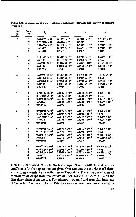
TABLE 4.3b. Distribution of mole fractions, equilibrium constants and activity coefficients (mixture I).

Plate

W 1

2

3

4

5

6

7

Comp. (0

1 2 3 4 5

1 2 3 4 5

1 2 3 4 5

1 2 3 4 5

1 2 3 4 5

1 2 3 4 S

1 2 3 4 5

**

0.485877 x 102

0.612908 x 101

0.106234 x 102

0.776195 0.734818

0.881583 X 102

9.71738 0.220317 X 102

2.86482 0.954967

0.950757 X 102

0.103400 x 102

0.242276 x 102

3.36934 0.994540

0.958139 x 102

0.104055 x 102

0.244641 x 102

3.42473 0.998650

0.958921 x 102

0.104121 x 102

0.244889 x 102

3.43036 0.999043

0.959016 X 102

0.104129 x 102

0.244919 x 102

3.43098 0.999082

0.959032 X 102

0.104129 x 102

0.244923 x 102

3.43107 0.999076

X)i

0.1093 x 10-5

0.4916 x 10-1

0.2188 x 10-5

0.5969 x 10"* 0.9507

0.1417 x lO"7

0.5137 x lO"2

0.1022 x 10"6

0.2082 X lO"4

0.9948

0.1824 x lO"8

0.5827 x lO"3

0.7085 x lO"8

0.6203 x lO"5

0.9994

0.1682 x lO"8

0.1427 x 10-3

0.3140 x lO"8

0.1846 x 10-5

0.9998

0.1679 x 10-8

0.1004 x 10-3

0.2976 x 10-8

0.5771 x 10"6

0.9998

0.1679 X lO"8

0.9642 X lOr* 0.2969 x lO"8

0.2082 X 10-6

0.9999

0.1678 X lO"8

0.9604 x 10-1

0.2969 x lO"8

0.1010 x 10-6

0.9999

yn

0.5310 x 10-* 0.3012 0.2325 x \Q-* 0.4633 x 10"4

0.6985

0.1249 x 10-5

0.4991 x 10"1

0.2252 x lO"5

0.5965 x lO"4

0.9500

0.1734 X lO"6

0.6025 x lO"2

0.1716 x lO"6

0.2090 x lO"4

0.9939

0.1611 x 10-6

0.1484 x lO"2

0.7682 x 10-7

0.6323 x lO"5

0.9985

0.1610 x lO"6

0.1046 xlO"2

0.7289 x lO"7

0.1980 x 10-!

0.9989

0.1610 x 10-* 0.1004 x 10-2

0.7272 x 10-7

0.7144 x 10-6

0.9989

0.1610 x 10-« 0.1000'x 10"2

0.7272 X lO"7

0.3466 X 10"« 0.9989

rk

0.3112X102

3.725 0.2947 x 102

0.2975 x 103

1.005

0.4567 X 102

4.559 0.4523 x 102

0.7143 X 108

1.0000

0.4770 X 102

4.664 0.4753 x 102

0.7944 x 103

1.0000

0.4791 x 102

4.674 0.4777 x 102

0.8029 x 103* 1.0000

0.4794 x 102

4.676 0.4780 x 102

0.8038 x 103

1.0000

0.4794 x 102

4.676 0.4781 x 102

0.8039 x 103

1.0000

0.4794 x 102

4.676 0.4781 x 102

0.8039 x 107

1.0000

4.3 b the distribution of mole fractions, equilibrium constants and activity coefficients for the top section are given. One sees that the activity coefficients are no longer constant as was the case in TABLE 4.3a. The activity coefficient of methylacetate drops from the infinite dilution value of 47.94 to 31.12 on the first three plates from the top. For ethanol, 1-butanol and methylanthranilate the same trend is evident. In the .^-factors an even more pronounced variation

59

fr 2 £ 3

n E 5

6

F

8

9 / r

'M .999 * - i —

199

/ 1 '

1 '\

R = ( J.997 i i

nooic L + -

Legends: Mixture I Influence of reflux ratio on Methyl anthranitate distribution Feed: x, = 0.1635 x 10-6

x, = 0.434 x 10"* x3 « 0.7291x10-7 Xt, : 0.237 xlO

10" 10" 10" 10" 10" 10" 10" 10'

FIG. 4.4. Influence of internal reflux ratio (R) on the composition distribution of methylanthrani-late, mixture I (MCDTG-programme).

appears, because the bubble temperatures of the three top plates are lower than in the preceeding example. The Abactor of methylanthranilate drops beneath unity on the top plate, which is the reason for the maximum in the composition distribution curve. The influence of the reflux ratio will be illustrated with the same mixture. In FIG. 4.4. results for the methylanthranilate distribution over the column are given, when the feed composition in TABLE 4.1 is distilled. The specifications were the same as given in TABLE 4.2, except for the reflux ratio wich was varied from 0.997 to 0.9995. The reboil ratio resulting from the last choice is 515.38%, which of course hardly represent economical operational conditions. However the influence of the reflux ratio increase on the com­position distribution of methylanthranilate is quite evident. A recovery of 99.5% of the methylanthranilate is achieved when R = 0.9995, but at the expense of a high steam consumption.

Finally the influence of the thermal condition of the feed when all other variables are kept constant (TABLE 4.2) was considered. To this end two distillations were calculated, with q = 0.5 and q = 1.0. The reboil ratio in the case q = 0.5 was 52.56% and when q = 1.0 this ratio is 102.56%. Again how­ever, the steam consumption is not constant as the reboil ratio varies strongly. The stripping action of the bottom section is increased by increasing q, this may be seen from FIG. 4.5, where the concentration distribution of methylanthrani­late is plotted against the plate number. The last situation, with q = 1, was dis­cussed by ROGER and TURKOT. The distribution calculated by MCDTG is in con­currence with their results. The higher steam consumption, tantamount to the choice q = 1 with constant other parameters, could be reduced by using the

60

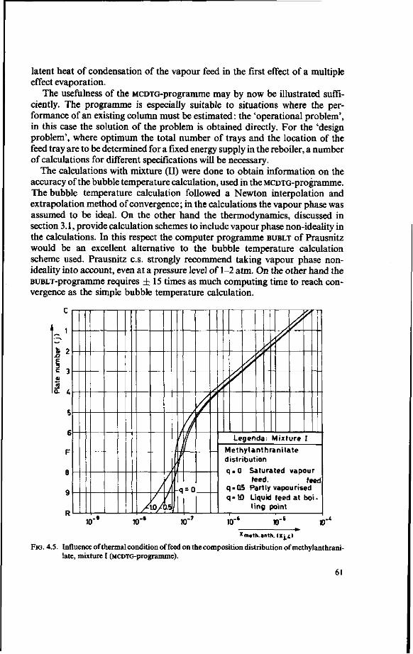
latent heat of condensation of the vapour feed in the first effect of a multiple effect evaporation.

The usefulness of the MCDTG-programme may by now be illustrated suffi­ciently. The programme is especially suitable to situations where the per­formance of an existing column must be estimated: the 'operational problem', in this case the solution of the problem is obtained directly. For the 'design problem', where optimum the total number of trays and the location of the feed tray are to be determined for a fixed energy supply in the reboiler, a number of calculations for different specifications will be necessary.

The calculations with mixture (II) were done to obtain information on the accuracy of the bubble temperature calculation, used in the MCDTG-programme. The bubble temperature calculation followed a Newton interpolation and extrapolation method of convergence; in the calculations the vapour phase was assumed to be ideal. On the other hand the thermodynamics, discussed in section 3.1, provide calculation schemes to include vapour phase non-ideality in the calculations. In this respect the computer programme BUBLT of Prausnitz would be an excellent alternative to the bubble temperature calculation scheme used. Prausnitz c.s. strongly recommend taking vapour phase non-ideality into account, even at a pressure level of 1-2 atm. On the other hand the BUBLT-programme requires ± 15 times as much computing time to reach con­vergence as the simple bubble temperature calculation.

k £2 E § a

/

/

\a/

;

J -

).5

^

t q = 0

Legenda. Mixture I

Methylanthranilale distribution q.O Saturated vapour

teed. feed q-05 Partly vapourised q-1£

— i —

) L li

qi "«

id 1 P

feed oint

at 5oi-

10 . 9 10" 10" 10" 10" »-

xm«th.anth. (Xj 4)

FIG. 4.5. Influence of thermal condition of feed on the composition distribution of methylanthrani-late, mixture I (MCDTG-programme).

61

The two methods were compared in the following way. First, for mixture II, a distillation was calculated with the MCDTG-programme using the specification given in TABLE 4.4.

TABLE 4.4. Specification of distillation calculation, mixture II.

F D 1 R(L/V) Rext N f P

= = = = = = = =

100. 5. 0. 0.

499. 8. 5.

(moles/ (moles/

1.0 (atm)

sec) sec)

Composition of feed. 1. methanol 0.25x10"' 2.2-heptanone 1.0x10"' 3. 1-octanol l .OxlO"4

4. water 0.974998

Then the BUBLT-programme was used to calculate bubble temperatures and vapour phase compositions from liquid compositions on each plate. The results are condensed in TABLE 4.5 and in the FIGURES 4.6-4.8.

From the table it is clear that, for 1-octanol especially, there are significant deviations between the two procedures. The error in a calculation from plate to plate is amplified strongly: an error of about 10% may result from five successive calculations, which are accurate to 2% and of 30% when the error per computation is 7.5%. In FIG. 4.7 the fugacity coefficients <p\ are plotted as a function of the tray number. The coefficients are almost constant, but, con­siderably lower than unity. One could therefore suggest using a constant value

u~.

375

370

36S

360

355

350,

/

V i

A =

O =

^'

Thie me( BUE

e Ge MCD LT p

ddes TG) rogr

Prog

amm

ram-

e —

1.000

0950

0.900

Water

Methanol

| 1 2-Heptan one

1- Octanol

Plate number(j) Plate number(j)

Fig. 4.6. Bubble temperature as a function of plate number (BUBLT-programme).

FIG. 4.7. Fugacity coefficients (<j>0 as a func tion of plate number (BUBLT-programme).

62

1

Water

Methanol

<; -2400

- 2500

-2600

-2700

-*BUUJ

>

>

I 2-Heptanone

-4000

-4100

-4200

•4300

•4400

4S00

1-0cta no I

8

Rate number! j )

FIG. 4.8. The second virial coefficient (Bu) as a function of plate number (BUBLT-programme).

for 9^ throughout the column, which is calculated after the first iteration cycle. The formula* for KJt becomes then (compare equation 4.8):

which means that for components with a low value for (pf the vapour phase mole fraction is underestimated when this phase is assumed to be ideal. The

63

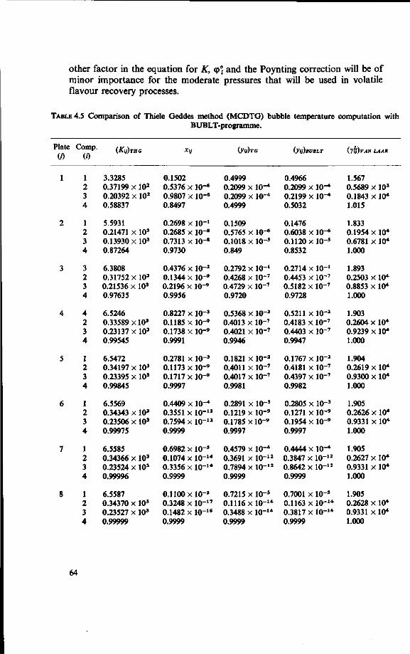
other factor in the equation for K, (p° and the Poynting correction will be of minor importance for the moderate pressures that will be used in volatile flavour recovery processes.

TABLE 4.5 Comparison of Thiele Geddes method (MCDTG) bubble temperature computation with BUBLT-programme.

Plate (/)

1

2

3

4

5

6

7

8

Comp. (0

1 2 3 4

1 2 3 4

3 2 3 4

4 2 3 4

1 2 3 4

1 2 3 4

1 2 3 4

1 2 3 4

(ATy)rHC

3.3285 0.37199 x 102

0.20392 x 102

0.58837

5.5931 0.21471 x 103

0.13930 x 103

0.87264

6.3808 0.31752 x 103

0.21536 x 103

0.97635

6.5246 0.33589 x 103

0.23137 x 103

0.99545

6.5472 0.34197 x 103

0.23395 x 103

0.99845

6.5569 0.34343 x 103

0.23506 x 103

0.99975

6.5585 0.34366 x 103

0.23524 x 103

0.99996

6.5587 0.34370 x 103

0.23527 x 103

0.99999

Xi]

0.1502 0.5376 X 10-6

0.9807 X 10"6

0.8497

0.2698 x 10"1

0.2685 X 10-" 0.7313 X 10-" 0.9730

0.4376 X lO"2

0.1344 X10-9

0.2196 X lO"9

0.9956

0.8227 X 10"3

0.1185 X lO"9

0.1738 X 10-9

0.9991

0.2781 X lO"3

0.1173 x 10-9

0.1717 X 10-9

0.9997

0.4409 x 10-* 0.3551 x lO"12

0.7594 x lO"12

0.9999

0.6982 X lO"5

0.1074 X lO"14

0.3356 x 10-14

0.9999

0.1100 x 10"5

0.3248 x 10-17

0.1482 x lO"16

0.9999

(yu)TG

0.4999 0.2099 X 10"4

0.2099 X lO"4

0.4999

0.1509 0.5765 x lO"6

0.1018 x lO"5

0.849

0.2792 x 10"1

0.4268 x 10~7

0.4729 x lO"7

0.9720

0.5368 x 10-2

0.4013 x lO"7

0.4021 x lO"7

0.9946

0.1821 x lO"2

0.4011 xlO-7

0.4017 x lO"7

0.9981

0.2891 x 10"3

0.1219 x 10-9

0.1785 x 10-9

0.9997

0.4579 x 10"4

0.3691 x 10~12

0.7894 x 10~12

0.9999

0.7215 x 10-' 0.1116 XlO"14

0.3488 x lO"14

0.9999

(yij)BVBLT

0.4966 0.2099 x 10-4

0.2199 x 10"4

0.5032

0.1476 0.6038 x 10-« 0.1120x10-' 0.8532

0.2714 x 10-1

0.4453 x lO"7

0.5182 x lO"7

0.9728

0.5211 XlO"2

0.4183 x lO"7

0.4403 x lO"7

0.9947

0.1767 x 10"2

0.4181 x lO"7

0.4397 x lO"7

0.9982

0.2805 x lO"3

0.1271 x 10~9

0.1954 x 10-9

0.9997

0.4444 x 10"4

0.3847 X 10-12

0.8642 x 10-12

0.9999

0.7001 x 10"5

0.1163 xlO"14

0.3817 x lO"14

0.9999

{yll)vAH LAAR

1.567 0.5689 x 103

0.1843 x 104

1.015

1.833 0.1954 x 104

0.6781 X 104

1.000

1.893 0.2503 x 104

0.8853 x 104

1.000

1.903 0.2604 x 104

0.9239 x 104

1.000

1.904 0.2619 X 104

0.9300 x 104

1.000

1.905 0.2626 x 104

0.9331 x 104

1.000

1.905 0.2627 x 104

0.9331 x 104

1.000

1.905 0.2628 x 104

0.9331 x 104

1.000

64

4.3. PLATE EFFICIENCIES IN MULTICOMPONENT DISTILLATIONS

4.3.1. Introduction The efficiency of transfer of a component i at a certain location (dOJ on a

plate in a distillation column (j) is commonly expressed as theMurphree point efficiency:

En,a = n-yi+i.i ( 4 2 1 )

In this equation yj, denotes the time smoothed (") vapour phase mole fraction of component i leaving plate j on a surface element dOa. The yjf denotes the time smoothed vapour phase mole fraction on plate j in thermo­dynamic equilibrium [at the pressure P,otj of plate j] with the time smoothed bulk liquid composition in a volume element A,- dOa, where A, is the liquid height at the same location AOa:

n = jJHTj;xli=l. n-l) Ft (T». ^ = ^ . ^ ^ ^

with

X/i — j— I •*# d A . (4.23)

The temperature T] is the bubble temperature of the liquid mixture with composition: xj j ; i = l,n.

The efficiency of an entire plate, most commonly defined as the Murphree plate efficiency or simply the 'Murphree efficiency' is expressed by an analo­gous equation:

, = <?*>-<?*»•'> . (4.24) \y%]-<yj + i,t>

In this equation <y}i> is the surface averaged (< >) , time smoothed (") vapour phase mole fraction of component i emerging from plate j :

<yjt> = J— JT JJrdO. . (4.25) Utot.j

Om j is the total surface of plate y available for phase contact. The [)$] is the vapour phase concentration of component / in thermodynamic equilibrium with the average composition of the liquid leaving plate j : [xJt], i= l,n; the pressure being Pm, j The [xjt] are defined by the 'cup mixing' relation:

[xji] = ~ ^ • <xjt v d>0d *), (4.26)

65

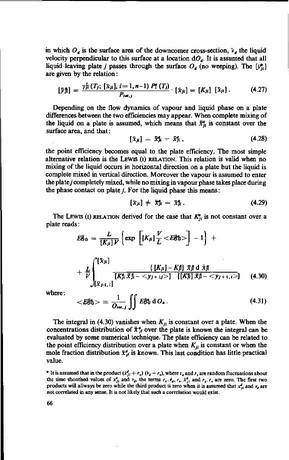
in which Od is the surface area of the downcomer cross-section, vd the liquid velocity perpendicular to this surface at a location dOd. It is assumed that all liquid leaving plate j passes through the surface Od (no weeping). The [>*(] are given by the relation:

m] = ykmnxMit-hn-DFtm. fe] = [Kji] {-Xjt] ( 4 27 ) "tot,)

Depending on the flow dynamics of vapour and liquid phase on a plate differences between the two efficiencies may appear. When complete mixing of the liquid on a plate is assumed, which means that x^t is constant over the surface area, and that:

[*;.] = S* = xj,, (4.28)

the point efficiency becomes equal to the plate efficiency. The most simple alternative relation is the LEWIS (I) RELATION. This relation is valid when no mixing of the liquid occurs in horizontal direction on a plate but the liquid is complete mixed in vertical direction. Moreover the vapour is assumed to enter the plate./ completely mixed, while no mixing in vapour phase takes place during the phase contact on plate/ For the liquid phase this means:

[xn] f 5* = S*. (4.29)

The LEWIS (I) RELATION derived for the case that AJ( is not constant over a plate reads:

L_ [Kji] V

MG = TE^TT? (exp [[*,<] £ <E&b>\ - 11 +

^ V

where:

Vxji] {[Kji] - Kfi X]l d Xjl

[K]iX]i-<yj + u>] l[X&]xfi-<yj + i.i>] (4.30) J[Xj-l,i]

<EWb> == -J— f f Ei&dOa . (4.31) V tot.j J J

The integral in (4.30) vanishes when KJt is constant over a plate. When the concentrations distribution of x't over the plate is known the integral can be evaluated by some numerical technique. The plate efficiency can be related to the point efficiency distribution over a plate when KJt is constant or when the mole fraction distribution x"i is known. This last condition has little practical value.

* It is assumed that in the product (JCjf + rx) (vd + rv), where r, and rv are random fluctuations about the time shoothed values of Xj, and vd, the terms rx.vd, rw.x'n and rx.rv are zero. The first two products will allways be zero while the third product is zero when it is assumed that x4^ and vd are not correlated in any sense. It is not likely that such a correlation would exist.

66

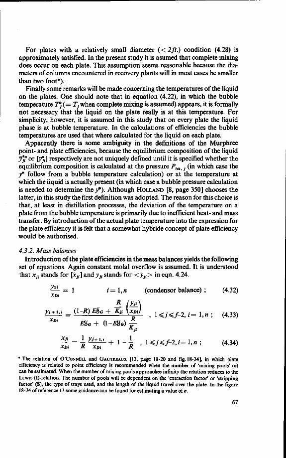
For plates with a relatively small diameter (< 2ft.) condition (4.28) is approximately satisfied. In the present study it is asumed that complete mixing does occur on each plate. This assumption seems reasonable because the dia­meters of columns encountered in recovery plants will in most cases be smaller than two foot*).

Finally some remarks will be made concerning the temperatures of the liquid on the plates. One should note that in equation (4.22), in which the bubble temperature Ttt

](=TJ when complete mixing is assumed) appears, it is formally not necessary that the liquid on the plate really is at this temperature. For simplicity, however, it is assumed in this study that on every plate the liquid phase is at bubble temperature. In the calculations of efficiencies the bubble temperatures are used that where calculated for the liquid on each plate.

Apparently there is some ambiguity in the definitions of the Murphree point- and plate efficiencies, because the equilibrium composition of the liquid y*" or [p*f] respectively are not uniquely defined until it is specified whether the equilibrium composition is calculated at the pressure Ptot<i (in which case the y* follow from a bubble temperature calculation) or at the temperature at which the liquid is actually present (in which case a bubble pressure calculation is needed to determine the y*). Although HOLLAND [8, page 350] chooses the latter, in this study the first definition was adopted. The reason for this choice is that, at least in distillation processes, the deviation of the temperature on a plate from the bubble temperature is primarily due to inefficient heat- and mass transfer. By introduction of the actual plate temperature into the expression for the plate efficiency it is felt that a somewhat hybride concept of plate efficiency would be authorised.

4.3.2. Mass balances Introduction of the plate efficiencies in the mass balances yields the following

set of equations. Again constant molal overflow is assumed. It is understood that Xji stands for [Xjt] and yJt stands for <yJt> in eqn. 4.24.

^ - = 1 i=\,n (condensor balance) ; (4.32)

A (yjL\ XDi

yj+i

XDi mG+ (I-EUG)^ (4.33)

•The relation of O'CONNELL and GAUTREAUX [13, page 18-20 and fig. 18-34], in which plate efficiency is related to point efficiency is recommended when the number of 'mixing pools' (n) can be estimated. When the number of mixing pools approaches infinity the relation reduces to the LEWIS (I)-relation. The number of pools will be dependent on the 'extraction factor' or 'stripping factor' (S), the type of trays used, and the length of the liquid travel over the plate. In the figure 18-34 of reference 13 some guidance can be found for estimating a value of n.

67

* (»-i.t\

^ = A*-' + (i-AV') it ' ' = 7 ' " ' ( f e e d t r a y ) ; ( 4 3 5 )

*zli! = I #L + 1 - I . , / = l,» , (feed tray). (4.36)

For the stripping section the balance equations read:

j N + l . i

XWi

n XWi

= E%ol,i KN-nj , i=\,n, (reboilerbalance); (4.37)

- = B— h/?- l) H (l-Eoa), i=l,n,f^j ^ N; (4.38)

^ = I ^ + ! " W ' / = !«" • ' < ' < * ( 4 3 9 )

JC^rj • " xWi **•

Starting at the condensor equations (4.32) to (4.36) are used to calculate the vapour and liquid composition ratios down to the (f-1) 'th tray as well as the vapour composition ratio on the feed tray. Commencing at the reboiler, vapour and liquid composition ratios up to the feed tray are calculated using equations (4.37)-(4.39).

When separated components are anticipated, as one is forced to do in flavour distillations, a different set of equations is obligatory. Introduction of the definition of the Murphree efficiencies into equations (4.11) and (4.12) gives the following equations for separated heavy and separated light components respectively:

XW\

l- = K»m0*\i-gL+ryj^ +(I-EU mid, i L \_ WxWi W xwi J xwt

U;</-1 (4-40)

yi + ui = l . r R (yA ,D( FxFi\\ Xm \i+JL(l_i]\ \KjiMc \x>>i/ V \ DxJ]

,l+f<j£N+l. (4.41)

The first equation is used for a separated heavy component in the top section, the second for a separated light component in the bottom section. The liquid phase mole fractions are given by the following equations.

For separated heavy components in the rectification section:

^ = f (l-£l) + I »L , f = 1,1, , 1 <j*f-l; (4.42) xwi L \ Wxwi) R xWi

68

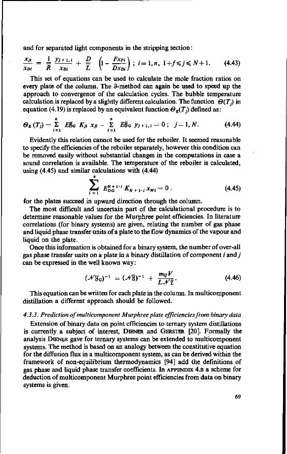
and for separated light components in the stripping section:

XJI _ _j_ yj + i,i , D / , FXFI

Xpi R XDi + I ( i - ^ ) : ' - L - . i + / ^<^+ i . (4.43)

This set of equations can be used to calculate the mole fraction ratios on every plate of the column. The S-method can again be used to speed up the approach to convergence of the calculation cycles. The bubble temperature calculation is replaced by a slightly different calculation. The function ©(Tj) in equation (4.19) is replaced by an equivalent function @E(Tj) defined as:

0E(Tj)=2 EtiaKjiXji- E E%G yj + i,t = 0 ; j=l,N. (4.44) i = l i = l

Evidently this relation cannot be used for the reboiler. It seemed reasonable to specify the efficiencies of the reboiler separately, however this condition can be removed easily without substantial changes in the computations in case a sound correlation is available. The temperature of the reboiler is calculated, using (4.45) and similar calculations with (4.44)

R

Z EU1,iKN + 1,ixwi=0. (4.45) i = i

for the plates succeed in upward direction through the column. The most difficult and uncertain part of the calculational procedure is to

determine reasonable values for the Murphree point efficiencies. In literature correlations (for binary systems) are given, relating the number of gas phase and liquid phase transfer units of a plate to the flow dynamics of the vapour and liquid on the plate.

Once this information is obtained for a binary system, the number of over-all gas phase transfer units on a plate in a binary distillation of component i and j can be expressed in the well known way:

(WoY1 =(MTX + j ^ . (4.46)

This equation can be written for each plate in the column. In multicomponent distillation a different approach should be followed.

4.3.3. Prediction of multicomponent Murphree plate efficiencies from binary data Extension of binary data on point efficiencies to ternary system distillations

is currently a subject of interest, DIENER and GERSTER [20]. Formally the analysis DIENER gave for ternary systems can be extended to multicomponent systems. The method is based on an analogy between the constitutive equation for the diffusion flux in a multicomponent system, as can be derived within the framework of non-equilibrium thermodynamics [94] add the definitions of gas phase and liquid phase transfer coefficients. In APPENDIX 4.B a scheme for deduction of multicomponent Murphree point efficiencies from data on binary systems is given.

69

Equation (4.46) is thus replaced by the matrix equation:

[NOG]-1 = [NG] " 1 + [S] • [NL]~l ; [S] = £ [m] . (4.47)

in which [N0G], [NG], [NL] and [S] are (n-1) dimensional matrices for a sys­tem of n components. The components of these matrices can be evaluated from data on binary systems.

DIENER and GERSTER [loc. cit] showed that for a mixture of acetone, methanol and water the average deviation between measured and predicted efficiencies was about 8 efficiency %. Moreover it was found that, when the liquid phase resistence was less than 50%, the difference between a binary prediction method (no interactions between diffusion driving forces, tanta­mount to equation (4.46)) and the ternary method was of the order of 10%, from which it was concluded that for gas phase controlling systems the binary method predictions may be a reasonable approximation. However, in dis­tillations of systems of very volatile components, [m] will have large compo­nents and therefore the liquid phase resistance tends to become dominating. This is an indication that in these distillations the multicomponent efficiency calculation scheme in APPENDIX 4B might be profitable. On the other hand the liquid compositions encountered in flavour recovery mostly are dilute solutions of organic components in water. In this section a procedure to calculate [N0G] will be discussed. In the next section a simplified scheme for aroma distillations is proposed. The quantity m in (4.46) represents the slope of the 'equilibrium curve' one could draw by comparison of the vapour phase mole fraction in equilibrium with the bulk of the liquid phase to that in equilibrium with the liquid surface concentrations:

m = < ^ > - ^ r > . (4-48) [X i] - <XiS>

<y$> is the time smoothed (") and surface averaged (< >) equilibrium mole fraction with respect to a liquid with a composition equal to the bulk con­centration, <yf"> is the vapour phase mole fraction at the interface, in equi­librium with < jcj>*). When the difference between the bulk liquid phase com­position and the interface composition is limited to two of the components, one of which is considered to be the solvent, mt is the slope of the function y( = Kt

{pa, i= 1,«-1). Xi. In multicomponent distillation, however, the concentrations of all con­

stituents are changing, travelling from the bulk of the liquid to the interface, as all constituents are transferred. Using a vector notation, a diagonal matrix [m] is defined for each plate with components my = <5y m, as given below (the vector {Ax} has elements Ax t which are differences between bulk phase and interface compositions):

* For simplicity it is assumed that interfacial resistance is negligible; this is not quite correct as situations may arise where surface active species concentrate at the interface.

70

ma = 8* ^ Kk ({x + Ax}) (xk + Axk) - Ait ({x}) xk

where {x+ Ax} = {x} + {Ax}, with:

w (4.50)

K({x + Ax}) is a non-linear function1 of the vectors {x} and {Ax} Rewriting the expression gives:

m i t = Sik xk *«»+A«})-*({z}) + Kk ( { x + A x } ) . ( 4 .51)

This relation can be simplified when the curve yt = KjXt is very nearly straight on the interval between two successive trays (xy-^j J.1)(see section 4.3.3.).

When the differences between bulk liquid composition and interfacial com­position ({Ax}) are not too large, the total differential d A({x}) can be used in (4.51) yielding at constant T and P.

mik = ^Kk({x + Ax}) + xk (j^ [Kk({x})]jT +

/ = 1,1 + k T,P,xs,s + l,k J

+ Xk

or, in vector notation:

[m] = [K] + m + [DK] • [X]

(4.52)

(4.53)

[ X] is a matrix with elements Xy = dyXj, [K] has elements Ky = <50- ({x + + Ax}). The matrix [DK] is (n-l) dimensional with elements Dy.

n - l

(4.54) T,P,x ; 5 + i, /

n - l

This matrix vanishes for a binary system. The partial differentials occurring in (4.54) can be calculated straightforwardly from equation (4.9) and (3.31), e.g.:

/^({x})\ = P ?^ /ainyjA \ dxi ) T P x l+ (. P \ dxt / T, p,xhi + t

P ^ Z ^.m(l-^>,) y [0-Awfl-fr) _ Ail<t>i<t>n> \ +

y -4./< ^—J { V Aji . y> v4j, m = 1 ^ - j — * i ' m = 1 I *-> —7- Xj AmiLd

j Ay \ j Aij A, •*J\

71

-XX*>% \-7 = 1 * = 1 fAji

j,k+i V

Aij Uk

p p

</>j<t>i (4.55)

The complete expression for m* would become quite formidable indeed if all the partial differentials in [DK] were evaluated.

The {Ax} vector has a relation to [Ni], the average flux vector on a plate across the gas-liquid interface is (compare with 4B-10 in APPENDIX 4.B):

L {<J">} = [Id.] • {Ax} As

{Axe} (4.56)

The vector {Axci} has elements (xj-i,i-xj,i) for component i on plate 7 the index V stands for 'column'. Equation (4.56) yields:

{Ax} = [N i ] " 1 . {Axe}. (4.57)

Using this result the interactions matrix [DK] can be formulated as *):

[D*] [dx . [{Ax} {Ax}"1] =

§ ] • [{ [NL]-1 • {Axc}| W ] - 1 . {Ax,,} j " 1 . (4.58)

Recapitulating the theory of this section, one can say that in principle it is possible to calculate the matrix [NOG] for each plate in a distillation of multi-component mixtures. The procedure is, using (4.53) as a starting point, first to calculate the elements of the matrix [m ] from the activity coefficients, compo­sition of liquid phase and the mole fractions in the downcomers to and from the plate under consideration (complete mixing is assumed). This calculation is very involved; which is reflected by formula (4.55) combined with the equation (4.58) for the interactions matrix [DK].

The matrix [m], which is diagonal, is used in calculating [NOG] from equation (4.47). Use of this equation requires the matrices [Nt] and [NG] to be known. In principle these matrices can be evaluated from binary data on numbers of transfer units in gas and liquid phase. To this end correlations could be used e.g. the ones proposed by the Distillation Committee of the A.I.CH.E. Research Committee. For bubble cap columns the following correlations were recommended for binary systems (component / and j); PERRY [13; 18-19]:

jry 0.776 + 0.116 W„ - 0.290 Fn + 0.0217 L„ (4.59)

* The 'dyadic' product between two vectors {a} and {b} : [{a} {b} ] is a matrix with elements

72

JTH =(0.26 Fn + 0.15) (1.65 x 1 0 4 ^ ' ) T c L, (4.60) where: u

Zc = 1.65 + 0.19 Wn - 0.65 Fn + 0.020 L„ .

In these correlations Wn is the weir height (in.), the F-factor is defined as the superficial vapour velocity times the square root of the vapour density (ft./sec. (superficial) ^/lb./cu.ft.), L„ is the liquid flow rate per foot weir length (gal/min), ZL is the length of the liquid travel over the tray (ft.). ®1 is the liquid phase diffusivity (sq.ft./hr.). Limits of applicability of (4.59) and (4.60) were suggested to be:

Sc'J ~ 0.6 1.0 <F„ < 2.3 5.0 < Ln < 25.0 1 < W, < 5 1.3 < traylength < 3.8

The correlations assume complete mixing on the plates and zero entrainment level. Moreover the operating pressure of the column is limited by 0.5 < P< 6 atmospheres. Equation (4.60) is based on the penetration theory as k'l is assumed to be proportional to (@i) i.

The Jft and Jf% data might serve as a basis for calculations of elements of the matrices [ N L ] and [ NG] , using the 'compounding' rules of APPENDIX 4.B.

Data on the liquid and gas phase diffusion coefficients will mostly have to be determined from correlations as WILKE [63], WILKE AND CHANG [64] and WILKE AND LEE [65] for liquid and gas phase respectively. In the calculation of [ N L ] the binary diffusion coefficients 3>li are calculated by first determining STOKES-EINSTEIN factors from the WILKE AND CHANG correlations [64] and combining these factors using a non-ideality correction and an interpolation to the relative concentrations of the i andy components in the multicomponent mixture using the WILKE formula [cf.Perry, 13, p. 40-21]. For a multicom­ponent mixture of (say) 10 constituents the calculation of the matrices [ N L ] and [ N G ] thus becomes a formidable task. In the type of distillation where the liquid mixture essentially consists of a number of components in a dilute solution with the n-th component (designated n the solvent), the calculations can be simplified considerably. In the next section these simplifications will be discussed more elaborately.

4.3.4. Simplified calculation of {EOG}for aroma distillations The calculation scheme to calculate the efficiencies vector {EOG} from the

[NOG] matrix as given in APPENDK 4.B can be simplified considerably when the multicomponent mixture consists essentially of a solvent (designated with index n) and (n-l)constituents present at fair dilution.

In the first place the calculation of the matrix [G ] from the matrizant exp ( - [NOG] ) can be simplified. Secondly the determination of the elements NBG

from binary data becomes very simple. These two simplifications will be

73

discussed first in this section. Finally the most far reaching simplifications will be discussed which arise when the equilibrium curve is assumed linear over a range of concentrations as can occur on two successive trays in the column and when [NL] and [Nc] are given by:

[ N , ] = N U U ] . [NG] = NG [ U ] ,

which means that all constituents of the mixture have the same number of gas phase and liquid phase transfer units on each tray.

The requirement that the multicomponent diffusion coefficient (D*!) should reduce to the binary diffusion coefficient {Q)u) in a mixture when it becomes dilute in components /(/ =/= /', n) is expressed by:

( + i,n k + i

If we assume that the thickness of the stagnant boundary layer in the gas phase is about the same for each component, the second term on the R.H.S. of (4.62) approaches zero. This assumption seems to be acceptable, thus the flux equation is simplified to*):

{J"} = -c [D-]-{Vy}, (4.63)

where [D~ ] is a (n-7) dimensional matrix with components DS = dikf&h,. When (4.63) is valid, the following equation can be written by analogy:

{Jm} = [KOG] • { Ay} d / = ^ {d y} . (4.64) As

In this equation [KOG] is a (n-1) dimensional matrix with elements (KOG)I* = 5i(t(Koc)toi. Defining the [NOG] matrix by:

[KQG A,

. V J [NOG] - p p j • (4-65)

The solution of the differential equation (4.64) upon integration between 1 = 0 and 1=1 becomes assuming V and As being constant in the interval

{Ay}0= exp (- [NOG]) • {Ay}f. (4.66)

The matrizant exp (-[NOG]) can now be transformed easily, using Sylvesters theorem, to a matrix [G] because [NOG] is diagonal.

The eigenvalues of [NOG] are simply the diagonal elements. The adjoint matrix [A] of the characteristic matrix of [NOG] is now also diagonal with elements:

* Tacitly it is assumed that the gas phase is ideal.

74

• - I

Ay = Sij J J ty - N${G) . (4.67)

1 = 1 l+i

The differential (d A/d^) of equation (3c. 14) is given by:

dA = y d^ ,= 1

n w- Na«) i = i

(4.68)

Using these results in the Sylvester theorem assuming that all eigenvalues are distinct, the matrix [G] becomes simply a diagonal matrix with elements GtJ = Sifixp (-N8G). The Murphree efficiencies {EOG} are given by the vector:

{EOG} = {1} - [G] • {1} , (4.69)

or, omitting the vector notation:

EOG = 1 - exp (- N&G) ; ( i = l , » - l ) . (4.70)

For each plate this relation can be written for (n-1) components, the effi­ciency of the «-th component is not freely adjustable but can be calculated from the others.

The overall gas phase efficiencies needed in (4.70) thus are the diagonal elements of the matrix [NOG], defined in equation (4.47).

A further consequence of (4.62) is that the matrices [No] and [N t ] become diagonal in the limit. The result of these limiting forms is in essence that (4.47) degenerates to equation (4.46) with water as component 7 which can be written for all components i (i = l,n~l) and for each tray. The calculation of NG and Ni is to be done in the same way as indicated in the preceeding section, now only (n-1) of such calculations are needed as compared with (n-1)2. The concentration effect in the WILKE equation can be deleted, taking the diffusivity at infinite dilution from the WILKE-CHANG correlation as representative.

As anticipated in section 4.3.2. the matrix [m] can be calculated in a more convenient way when the equilibrium curve y(xt) = Ktxt is very nearly straight on the interval between two successive trays in the column. Mathematically this implies:

Kk ({x + Ax}) (xk + Axk) - Kk ({x» JH ~. Axk (4.71)

_ &({*+ Axc,}) (xk+ Axdk)-Kk({x})xk. — Axdk

Here { Axct} is defined as in equation (4.56). Using this approximation one can deduce for [m]:

[m]=[K,, ]+ p l ^ l . [X ] , (4.72)

75

[Kci] has elements Kciy = Sy Kj ({x + Axci}).

The matrix -r—- has elements: LAXc/J

di * ,({x+ Ax,,})-*;({x}) ( 4 ? 3 )

The elements of this matrix are easily calculated in the distillation calculation from the current estimates of the equilibrium constants and the composition distribution over the trays during the iteration cycles.

Finally the gas phase and liquid phase number of transfer units, equivalent to one tray will be regarded as equal for all components, the confluent form of Sylvesters Theorem (APPENDIX 4B) now must be used. Although this approxi­mation may seem to lack an acceptable base, one should keep in mind that the main factor causing differences in £J>G values for different constituents of the mixture is the occurrence of large differences in [m]-elements for different components, while differences in the Njj and IM'ii values for different com­ponents might lay within the accuracy limits of the correlation used. This statement may be substantiated by the following example. For instance when the correlation (4.59-60) is used, differences in Nj! and Ni£ for different com­ponents are caused mainly by differences in the diffusion coefficients. Extreme differences in diffusion coefficients give a factor of 1.5 say, which would result for N& or NZ in a factor 1.22. Taking an average diffusion coefficient in the Njj and Nj| correlation would result in a difference of ± 11°/0. A representative ratio of AT-values is for instance the ratio between 2-heptanone and methanol

which is about I ' 1=52. Bearing these arguments in mind in the computer

programme this final simplification was applied; it can however be removed easily when one has more accurate correlations at ones disposal to replace equations (4.59-60).

Summarising the assumptions made in the calculation scheme of POG' (i) The distillation contains a solution which is dilute in (n -1) components; (ii) The values for JTL and JYG are predicted with sufficient accuracy by the

correlations (4.59) and (4.60). Average diffusion coefficients are used; (iii) The equilibrium curve is essentially straight over a concentration interval

covering mole fractions in liquid phase on two successive trays in the column.

Formally all these assumptions can be relaxed as shown before, however the computations will become more and more involved and at the same time de­crease in feasibility.

The results of this section can be summarised as follows. For a multicom-ponent distillation a calculational procedure is proposed for estimation of efficiencies for each component from column dynamics and physical pro­perties of the components. Three levels of sophistication of calculations can be distinguished, the most simple of which is made acceptable for the special case

76

of dilute solutions of components with a very high relative volatility with respect to the solvent.

In the next section some sample calculations will be given to illustrate the scheme.

4.4. DISTILLATION CALCULATIONS WITH EFFICIENCIES INCLUDED

The calculation scheme described in section 4.3. was programmed; the programme is indicated by: MCDTG-EFF. The organisation of the programme is discussed in APPENDLX 4.c.

The correlations (4.59) and (4.60) were used in the programme. They can be replaced easily by other correlations of course. Three types of calculations will be discussed. Two calculations were performed with mixture II of section 4.2.: methanol, 2-heptanone, 1-octanol and water. The specifications of the calcu­lations are the same as given in TABLE 4.2. In addition data on the gas and liquid dynamics and dimensions of the column are specified (TABLE 4.6).

TABLE 4.6. Specification of column for distillation calculations with efficiencies included.

w. Fn

Ln

®L

zL Scg

= 2.0 = 0.8 = 40.0 = 0.36 x 1 0 " = 2.0 = 0.6

weir height [inch] F-factor (ft/sec (superficial) , / lb/cu. ft]*) [gal/min. (average liq. flow width, ft)]*) [sq. ft/hr] length of liquid travel [ft] Schmidt number gas phase [- ]

* Strictly speaking F„ and Ln are not constant over the whole column, although constant molal overflow is assumed. Corrections can easily be built in the computer programme.

Use of this specification results in 2.405 gas phase transfer units and 1.192 liquid phase transfer units for each bubble cap tray. The results of the two calculations which differred only in the methanol concentration in the feed, are given in FIG. 4.9 and 4.10, where the concentration distributions of the components are sketched and compared with the results from the equivalent ideal-tray calculations. In TABLE 4.7 composition distributions for mixture II are compared with the MCDTG programme.

The 'pinched in' regions for heptanone and octanol, that appeared in the ideal tray calculations disappear when efficiencies are included in the calcu­lations. The mole fractions of methanol, heptanone and octanol in the bottoms increased from 0.1100 x 10"5 to 0.7962 x 10"3, 0.3248 x 10"17 to 0.9640 x 10 1 0 and from 0.1482 x 10~16 x 0.1461 x 10"9.

The distribution of Murphree point efficiencies along the column is very instructive; in FIG. 4.11-12 the distributions for the calculations with x F,methanoi = 0.25 x 10"1 and 10"6 are given. The constituent with the highest AT-value (2-heptanone) always appears to have the lowest point efficiency because the effect of the liquid phase resistance is very high. The least volatile constituent (water) has an efficiency of 90.97% which is constant all over the

77

FIG. 4.9. Distillation calculation of mixture II (secion 4.2.) with MCDTG-EFF programme compared with MCDTG programme.

C. 1

c 2 3 n

CL

..ideal" reboiler efficiencies reboiler

, . • • . • ' ' •

-,' '*•'

/ > • "

sT'f 1 1 y

i j

. m '

^t~

:" : ' ' '

10* 11 11

10*

-, •

\ 1 \ l

'""

/j

i s

.102

.10^

.."'

/

s s 4 •

/.

—*2 •

— X V

/

/

>*''

102

102

/

r^

'""

,' s

s

i A

- - ' - • ' '

•

/ / X |

/ !

i ft 7 Cor

" X 1 « x2 .

V

'/

f

, ^

"i U / f

v

Legenda Mixture I I :

-}MCDTG-EFF -- MCDTG nposition of

feed: 0.25.10''

1. D.10 -6

10" 10" 10 ,-S 10" 10" 10" 10" Xii

FIG. 4.10. Distillation calculation of mixture II (section 4.2.) with MCDTG-EFF programme com­pared with MCDTG programme.

78

II

k.

a

1

° • 3 ? S 5 I 3 U S c i c

r

II

c IS

V

II

8

V

1 3

\ eg n

"5> c _o c •0 a « I

\

3 c

~ * • " *

U

3 C

• 10

a.

> V, S c u '3

s • ta.

(3 O O.

8 J3

t

a o c o 3

•c

a <N

•<t

o u.

2 s K

s <<-. O

a u at o §

• ^

j d

CO

T3

.s

3

U

£

^ se

O

II

J=

s u.

X

9 0 .

Wat

er ( i

= 4 )

J II

o X

o c

7

(M II

f t O

>T

S o c 10

o. 0)

'l

I I

o c 10

2

"„ fc £ o 5

u 8 E '3 "•" a £, .2 *3 « 6 2 ° 3 s * 11

O 8 e &^

a-a

3 § « .•2 -3 w .2 u ° Q-S II

s s § 3 6

9 0 -

79

TABLE 4.7. Comparison of MCDTG programme with MCDTG-EFF programme

MCDTG plate

( / • )

1

2

3

-programme component

(0

1 2 3 4

1 2 3 4

1 2 3 4

* j .

3.3285 x 10° 0.37199 x 10* 0.20392 x 10* 0.58837

5.59315 0.21471 x 103

0.13930 x 103

0.87364

6.38088 0.31752 x 103

0.21535 x 103

0.97635

MCDTG-EFF-programme

1

2

3

1 2 3 4

1 2 3 4

1 2 3 4

3.21163 0.17801 x 10* 9.82645 0.65199

4.75675 0.77356 x 10* 0.46892 x 10* 0.84364

5.62641 0.15940 x 103

0.10217 x 103

0.92993

Xji

0.1502 0.5376 x 10"6

0.9807 x lO"6

0.8497

0.2698 x lO"1

0.2685 x 10~8

0.7313 x 10-8

0.9730 x 10

0.4376 x 10"* 0.1344 x 10~9

0.2196 x lO"9

0.9956

0.2461 0.6939 x 10-5

0.7323 x 10-* 0.7538

0.2216 0.2379 x lO"5

0.2518 xlO"5

0.8783

0.6254 x 10-1

0.8854 x 10-6

0.9320 x lO"6

0.9374

y»

0.4990 0.2000 x 10"* 0.2000 x 1 0 ^ 0.4999

0.1509 0.5765 x lO"6

0.1018 x 10"' 0.8490

0.2792 x 10-1

0.4268 x 10"7

0.4729 x lO"7

0.9720

0.4848 0.1999 x 10"* 0.1999 x 1 0 ^ 0.5150

0.2466 0.6965 x 10-5

0.7349 x 10~5

0.7533

0.1223 0.2414 x lO"5

0.2553 x 10"5

0.8776

i-ft)

1.567 0.5689 x 10s

0.1843 x 10* 1.0150

1.8330 0.1954 x 10* 0.6781 x 10* 1.0000

1.8930 0.2503 X 10* 0.8853 x 10* 1.0000

1.4120 0.2470 x 103

0.7901 x 103

1.0420

1.6218 0.7444 x 103

0.2437 x 10* 1.0100

0.1747 X 101

0.1342 x 10* 0.4536 x 10* 1.0020

column because the resistance to mass transfer is mainly in the gas phase. The efficiencies of the organic components are the highest in the top of the column (where the /w-values for the respective components take their lowest values). In the bottom section all the efficiencies are almost constant, but at their lowest values.

In FIG. 4.13 the mole fraction distribution of methylanthranilate over the column is given compared with the analogeous calculation with the MCDTG-programme. It is clear from this FIG. 4.13 that efficiencies must be included in distillation calculations for flavour recovery units as ideal plate calculations lead to an underdesign of a column. In FIG. 4.14 the efficiency distribution for mixture I is given in this distillation.

The efficiency distribution in the top section has the same pattern as was the case in the calculations with mixture I. However, the reflux ratio in the bottom

80

1*

u .-. 1 b. 01

1 2 c 01

5 3

U

5

6

F

8

9

R

i

/

/ / / / i

1

/ / /

/ /

/

/

/

/ s /

J 1

• •

•

s

/ / / s

s

Legends-. Mixture

Methyl anthranilate distri­

bution (xF4= 0.237x10"*)

MCDTG - programme( )

MCC )T6 - EFF. programme — -)

10" 10" 10_ io-' Xmtlh.anth. ' x j ,« )

FIG. 4.13. Concentration distribution of methylanthranilate for a distillation calculation with MCDTG-EFF programme, compared with MCDTG programme.

section is much lower. Therefore the efficiencies in the bottom section are much higher, despite the larger liquid phase resistance in this section.

The conclusions of this section are: (i) The inclusion of efficiencies in the calculations in the way proposed in

section 4.3 is possible and gives acceptable results. The only weak point is that the correlations for Jf% and Jft need not to be the best ones for these calcu­lations. It is important to develop reliable correlations for Jf^ and Jfi for the tray types used frequently in volatile flavour recovery columns;

(ii) The calculations with ideal trays give wrong concentration distributions over the column when the gas- and liquid phase numbers of transfer units are not high. For very volatile components especially the effect of the liquid phase resistance becomes very high, resulting in the largest deviations for these components;

(iii) Because the concentration gradients over the column are less pronounced

81

1.0

US

08

07

0.6

05

(U

uu

02

0.1

0

1.BuUnol(i=3>

ithylacc >tate(i =

\

) \ \

Water(i = 5>

- i - D u i s n g i i " M i l l - 31

Ethy(<

anthra

cetate (

nitated

*10)(i=1) 11 1 1

Ethanol(i = 2 )

y

_ -

9 8 1

Plate number ( j ) FIG. 4.14. Murphree efficiency distributions for mixture I (section 4.2) as calculated by MCDTG-EFF

programme.

as those calculated with the MCDTG-programme, deviation of the activity coefficients from their infinite dilution values is no longer limited to the top plates of the column but is extended to a larger region. Moreover the activity coefficients of the liquid mixture on the first plate can show larger deviations than calculated with the ideal tray programme (MCDTG) because the liquid is more concentrated in organic components. This situation is illustrated by TABLE 4.7 where A-values, activity coefficients and mole fractions for the first three plates are compared for the two calculations with mixture II (x vjmeoumoi = 10"6). Therefore the need to include concentration dependence of activity coefficients in a particular problem will be even more pronounced than what would be concluded from calculations with the MCDTG-programme.

(iv) There are two opposite effects of the volatility of a component on the degree of separation for a component. The favourable effect is that the stripping factor (Sji) becomes larger when a component is more volatile. A moderating effect on the degree of separation results from the decrease of the point ef-

82

ficiency with the increase of the volatility (caused by the decrease of the overall number of transfer units). For plates with a large diameter, where the plate efficiency is no longer equal' to the point efficiency this effect, however, is partly compensated by the increase of the ratio between plate efficiency and point efficiency with an increase of m.

The result of these counteractions is that even when the volatility of a com­ponent is very large, the component must be taken into account in the design of a flavour recovery plant as its ease of separation is only partly warranted by its volatility. This statement is, to some extent, in contrast with the remarks of ROGER AND TURKOT, [4].

83

5. E X P E R I M E N T A L PART

5.1. METHODS FOR DETERMINATION OF VAPOUR LIQUID EQUILIBRIA

The measurements of vapour liquid equilibria (VLE) in general does not need the measurement of the vapour composition. Thermodynamically a vapour/ liquid system is already completely specified if the composition of the liquid phase, the temperature and the total pressure are known by measurement [21, 46, 18]. The vapour phase composition can be calculated from rigourous thermodynamic relationships [VAN NESS, 21 ] such as described in section 3. However if one component is present at extremely low concentrations, the method requires extremely accurate measurements of composition, tempera­ture and pressure. For totally miscible systems this phenomenon is hardly a stumbling block because the behaviour of the system at very low concen­trations of either component can be accurately predicted from that at higher concentrations. If the system is partially miscible this is possible to a lesser extent, as it requires extension of the measured quantities in a two phase system to a region where only one liquid phase is present. There is some uncertainty as to whether it is allowed to extrapolate Van Laar curves for activity coefficients from a miscible to an immiscible region: GARNER and ELLIS, [62]; GILLILAND

and ROBINSON, [66]. A deviation from the Van Laar equations of the experi­mental data on systems approaching immiscibility has been observed; this could be due to entropy effects occurring on mixing. One cannot expect the excess entropy of mixing to be zero in partially miscible systems; this condition (A eS = 0) was used in the derivation of the Van Laar equations. If one is forced to measure activity coefficients in dilute solutions, a gas chromato­graphic method can be useful. The most attractive point is that the con­centrations of each component in the vapour phase can be measured simul­taneously, making the method especially useful for measurements on multi-component systems.

In literature measurements of activity coefficients of dilute solutions by gas chromatographic methods are reported. Essentially three methods can be distinguished, a 'direct' method and two 'indirect' methods, a stationary 'indirect' method and a dynamic 'indirect' method. A short description of the methods with subsequent evaluation will be given in the next sections.

5.1.1. The 'direct' method

In this method one of the components is used as stationary liquid phase of the gas chromatographic column. A small sample (in the order of 0.1-10.0 nl) of the second component is injected on the column. Measurement of the retention volume allows, after some corrections, for the calculation of the activity coefficient of the injected component present at infinite dilution in a binary mixture with the other component (the stationary phase). Details are given in several references: KwANTES and RIJNDERS [67]; DESTY and GOLDUP [68];

84

HOFSTEE, KWANTES and RUNDERS [69]; KEULEMANS [70]; EVERETT and STODDART [71, 72].

The activity coefficient at infinite dilution can be calculated from [see EVERETT and STODDART, 71 ]:

In rf" = In ( H - ̂ _ « . ( 5 l l _ g ) + <g= (2 *12 - *2 2 - KD. (5.1)

Index 7 indicates the volatile liquid and 2 the carrier gas. In deriving this equation it is assumed that Henry's law is obeyed and that equilibrium is maintained between vapour and liquid. Correction for deviations from these assumptions can be made if the retention volume (V°R) used in (5.1) is the retention volume extrapolated to zero flowrate and zero sample size. The two last terms at R.H.S. of (5.1.) are corrections for the gas phase imperfection and in essence require the second virial coefficients of the pure carrier gas and of the component as well as a cross term in the virial coefficient expansion to be known.

In literature the method was used for measurement of e.g. the activity coefficients of acetone, butanone-2, methanol and 1-butanol in water at temperatures of 40° and 60°C. Although this method seems attractive, it cannot be used to measure the influence of the liquid phase concentration on the activity coefficients, one of our main points of interest. However for measuring infinite dilution coefficients in binary systems the method has proved to be quite useful.

5.1.2. The 'indirect' dynamic method of Burnett

BURNETT [73] described a method of measuring partition coefficients in dilute solutions by gas chromatographic analysis of the vapour. He used a small saturation cell containing the liquid mixture to be investigated. Hydrogen gas was bubbled through, and the volume passed at any time during the experiment could be measured. At regular intervals samples were taken from the vapour-gas mixture emerging from the cell. Determination of the partition coefficient followed from a mass balance over the cell. One can derive the following rather general formula, assuming that the gas is not soluble in the solution and that complete phase equilibrium is attained:

dxi dxi +

[, + x'{wr>)](1-") . L {,+'i(w,)}(l-*)* -^i-nJvk- _ (52)

Here aty is the relative volatility between component i andy, W is the partial molar volume of component /, Vn the partial molar volume of the entraining

85

gas, Mi and M) molecular weights of solute and solvent respectively, <j> is the volumetric flowrate emerging from the cell, W{t) is the weight of solution in the cell at time /.

If the vapour is assumed to be an ideal gas, the first integral vanishes. When the solutions are very dilute and/or the molecul weights (Mi) and (Mj) do not differ substantially, in the second term the denominator part between braces is very nearly unity. When the rate of change of W(i) is constant (fi) one can simplify to:

From the result of the vapour analysis giving the corresponding solute concentration (xi), and measurement of /? by weighing the sample at regular intervals, the relative volatility a« can be determined from the slope of a double logarithmic plot of (5.3). If the solution is sufficiently dilute, so that the activity coefficient of the solvent is unity, and when the fugacities of the pure sub­stances are known, the activity coefficient of the solute can be calculated from:

BURNETT expressed his results in a partition coefficient, defined as mass of solute par unit volume of solvent divided by mass of solute per unit volume of the gas phase. This quantity can be transformed to an activity coefficient. His results (among other aqueous solutions of methanol, ethanol, 1-propanol, 1-butanol) are not in agreement with other data at the same temperature in literature. There is some doubt as to whether the small saturation cell BURNETT uses (liquid height 2 cm) is dimensioned properly for reaching a negligible deviation from the vapour liquid equilibrium. The arguments he uses to confirm that saturation was achieved are not very convincing (see APPENDIX 5.A).

5.1.3. A modified 'indirect' method and its limitations

The method of BURNETT was modified to ensure complete saturation of the hydrogen gas. A better approach of equilibrium can be achieved by increasing the height of the liquid in the saturation cell. This means that the amount of liquid solution under investigation must be increased. As a consequence the decrease of the peak on the chromatogram with time is diminished con­siderably, which means that the formula (5.3) becomes less useful.

Both L.H.S. and R.H.S. of approach zero. This implies that the activity coefficients and the relative volatility must be calculated directly from the peak area.

It will be shown (APPENDIX 5.A) that a column height of approximately 50 cm will be sufficient for the equilibration of a solution and 20 cm for a pure liquid (where the only resistance to mass transfer is in the gas phase).

In the beginning this dynamic method was used in the present research, and

86

it gave acceptable results when solutions of 1-butanol were used to test the apparatus. However when 1-decanol solutions were analysed a serious short­coming of this method was discovered. In FIG 5.1 the results for the activity coefficients of decanol as determined with this indirect dynamic method are given. An increase in the activity coefficients for smaller concentrations was calculated in .a concentration region where such an increase is physically impossible. The explanation of the phenomenon was found in considering the adsorption characteristics of chain molecules like decanol at a gas liquid interface. It is well known in surface chemistry that alcohol molecules in an aqueous solution tend to concentrate at gas-liquid interfaces because this is energetically favourable [46]. If we follow a gas bubble traveling through an alcohol solution, the bubble surface will be concentrated with alcohol mole­cules, with their polar group in the water phase and the chain of C-atoms in the gas phase. When the bubble reaches the gas-liquid interface it will, though not necessarily instantaneously, collapse. When moreover the surface excess is very high the, suddenly diminished, gas-liquid interface results in a local over-concentration of the alcohol. The redistribution of molecules of the solute, necessary when a change in interfacial area takes place, is governed by dif­fusion. In this case it is a back diffusion to the bulk of the liquid, which is a slow process (Q>Y3 ~ 10"9m2/sec). From a recent paper [BAKKER, VAN BUYTENEN andBEEK,74] a rough idea can be formed of the times needed for such a process. The dimensionless surface excess is given for a flat interface of a stagnant liquid as a function of time:

10'

8

6

10' 8

6

10'

1

X J i

- . 4

•

1 1

i\ in 1

• • "" "~

nV y\- i n '

IU

Legsnda

Comparison off bubble column method with static method.

1 . Decanol Pentanone - 3

Xi

10"7 2 4 6 8 10-" 2 4 6 8 10"* 2 4 6 FIG. S.l. Measurements on 1-decanol and pentanone-3, static vs. dynamic method.

87

n- m. 1 - exp rt-n

where the surface excess riJ is given by: a da,; „

R r dc,

m erfc

T": C.Ly

(5.5)

(5.6)

For 1-heptanol: L = 3 x I0'6m, for l-hexanol7 x 10"7m and for ethanol 7 x 10"8 m. The characteristic times needed to reach a ratio (r0-r[f ])/(r0~r<» ) = 0.90 is respectively 0.3 sec, 15 msec and 1.5 ftsec. When the component is partially miscible with the solvent and the characteristic time is appreciable, circumstances are favourable for phase separation in cases where the surface excess after the surface reduction (r0'

J) considerably exceeds the solubility limits. Phase separation was in fact observed during measurements on 1-decanol-water solutions.

A well stirred, perfectly homogeneous solution of decanol in water far below the solubility limit of decanol in water STEPHEN and STEPHEN [75] showed small drops of a decanol-rich phase floating at the liquid surface after some time, when nitrogen gas was entrained. Moreover, tiny spatters of the bubble skins were collected in the dropcatcher (see FIG 5.2); these spatters consisted of a two phase liquid in the 1-decanol/water experiments.

Leaenda. 1 = Glass sinter plate

(20.4011) 2 - Drop catcher (a pad

of glass fibers)

3 = Goose neck

FIG. 5.2. Saturation cell, detail sketch.

This separation phenomenon gives the explanation of the measured beha­viour of the activity coefficient as a function of the concentration, because the measured partial vapour pressure is influenced strongly by the presence of separated drops of almost pure decanol. From FIG. 5.1 one can see that the slope of the lnyf-curve on a double logarithmic plot has a slope of approxi­mately in which means that the (apparent) vapour pressure is almost constant, irrespective of the concentration of the solution. In the plot measurements with pentanone-3 in water are also given, showing the same tendency, albeit less pronounced as could be expected. It was concluded from these phenomena that a dynamic method as described, is only accurate when the solutions have moderate values of the activity coefficients (< 50 say). Therefore in Burnett's measurements with C1-C4 alcohol solutions this phenomenon was of no influence.

5.1.4. The 'static'' method In view of the difficulties encountered with the application of the method

described in section 5.1.3, it was decided to use a static method: a way of pre­venting the concentrating effect due to entrainment. Another method of pre­venting the concentration effect would be to stir the liquid vigorously. However then still spatters of the bubble skins may collect in the drop-catcher inevitably necessary in the entrainment cell. The use of a static method also circumvents this source of error.

In a static method a quantity of liquid is stirred isothermally in a container with a considerable gas space. Initially this space is filled with nitrogen gas, then the container is allowed to equilibrate at atmospheric pressure. When the gas is saturated with vapour it is led through a sampling chamber by pushing it out of the container with a liquid mixture of the same composition and temperature. In the next section this method will be described more extensively.

5.2. DESCRIPTION OF THE ULTIMATE EXPERIMENTAL APPARATUS

5.2.1. The gas chromatograph Vapour samples were analysed with a Becker gas chromatograph, provided

with a flame-ionisation detector. The columns used were aluminium tubes (length 3 m) with an internal diameter of 0.4 cm. Two types of stationary phase were used: LAC-2-R-446 (Schuchardt GMBH, Munchen) and PEGS 728 (Carlo Erba). Both types of stationary phase were applied (10%) on 60-80 mesh Chromosorb-W solid support by standard methods. Both columns were present in the oven of the chromatograph, switching from one to the other was possible. In most experiments however the 'Ly4C'-column was used. The operation conditions of the chromatograph were: nitrogen carrier gas 20 cm3/ min., hydrogen gas flowrate 17 cm3/min, air flowrate 140 cm3/min. The temperature of the column was adapted to the physical properties of the components to be analysed.

Samples were introduced on the column, using a sample valve (Carlo Erba,

89

Flowmeter

Gas-chromatogra

Sample supply Flowmeter Sample supply

Gas-chromatograph

Carrier gas Carrier gas

Situation 1

FIG. 5.3. Schematic sketch of the sample loop (Carlo Erba).

Situation 2

6 way valve). In earlier experiments syringe sampling was used, however this method of sampling causes a relatively large random error as compared with the sample valve method [73]. The latter method is also considerably less laborious. The construction of the valve is sketched in FIG. 5.3. and 5.4. In situation 1 the carrier gas is led through a spiralised stainless steel tube with a volume of 3.6 cm3 before it enters the column, while the stream of vapour to be analysed flows out to the surroundings. In situation 2, the carrier gas flows directly to the column and the vapour flows through the stainless steel sampling tube. If one assumes the sample loop to be a perfect mixer*) with a volume of 3.6 cm3, a flow of 2 cm3/sec of vapour passing through, the time needed to attain a concentration of 99.9% of the final (equilibrium) concentration is 12.6 seconds. It was decided to choose an 'exposure time' of 30 seconds throughout the experiments. The possible influence of adsorption at the wall of the sample loop is discussed briefly in section 5.2.3. The sample loop was heated to 100 °C to reduce adsorption as much as possible.

The peak area were measured with a Disc Integrator which is accurate to ± 2.0% when the appropriate corrections are applied.

5.2.2. Standardisation of the relative retention volumes It has become customary in quantitative analysis of vapour samples with a gas

chromatograph to use an internal standardisation of the relative retention volu­mes. A constant amount of a reference substance is added to each sample by some device. The peak surfaces are normalised with respect to the peak surface areas of the reference substance. In literature several methods are suggested to provide a constant reference [MEIGH and CURRAH, 77; WEURMAN, 78]. In the *In reality the situation will be intermediate to a perfect mixer and a tube with Poisseuille flow, DANCKWBRTS, [76].

90

Silicone oil heating (100*0

1 ! ih jti

Sample tube

Thermo-couple

Heating jacket

Sample out i i Sample in

/ . , , s / s /

ii—"-"!-!—-—h * ' * ' ' ' ' *

' ; ; ; ; ; / / - i

Carrier gas out' ' Carrier gas in

FIG. 5.4. Sample loop + housing.

present study a method was used which allowed a sample of the internal standard to be drawn at the very moment of sampling.

In FIG. 5.5 the apparatus is sketched. A vapour stream with a constant concentration of iso-propanol was prepared by the following procedure. Nitrogen was entrained through a saturator flask (6) containing purest grade commercial iso-propanol ( MERCK P.A.).

The flow of vapour was measured by a precision flowrator (Q4). In a mixing chamber (8a) the vapour stream was diluted with a (measured) constant flow of nitrogen gas (Qi). The saturator was kept at a constant temperature of-14.9 ±0.02°C by means of a laboratory size cryostate (5). The temperature was chosen so low to circumvent problems associated with the mixing of two streams of very different flowrates. Moreover it was preferred to use a volatile substance as a reference because of its short retention time and consequent

91

small chance of interference between standard peak and the other peaks in the chromatogram. The height of the liquid level in the saturator (see FIG. 5.2) was ± 20 cm; calculations with the theory of APPENDIX 5.A. show that deviations from complete saturation are negligible in this case.

5.2.3. Calibration of the elution curves In order to allow for quantitative measurements the ratio between the area

of a peak and the area of the standard peak has to be correlated to the con­centration of the component in the vapour sample. Calibration curves were prepared for each component by preparing known concentrations in vapour phase and measurement of the peak area ratio (ki). The calibration curves are always straight lines over a concentration range of several decades, which is in concurrence with literature about the subject Mc. WILLIAM [79], WEURMAN [78], MAHEDEVANand STENROOS [81], BURNETT [73], KEPNER c.s. [80].

In FIG. 5.5 the apparatus is sketched. The experimental procedure was as follows. By suitable adjustment of the precision needle valves (4a) and (4b), a concentration was set. Flow (Q3) was entrained through a saturation cell exactly like that used for the internal standard.

Gaschromatograph

U.9°C

i"fPRCl

^JJ^ FIG. 5.S. Schematic flow sheets of the standardisation circuits for relative retention volumes and

elution curves.

92

The liquids used were all purest grade commercially available products, no further purification was attempted. Flow (Q2) and (^3) were mixed (8b), at the point of mixing the pressure was measured with a mercury manometer (9). From the mixer the vapour was led to the sample valve; an air vent (11) was mounted in this tube to be able to reduce the excess-pressure in the system when very low concentrations were prepared. The resultant flow downstream the air-vent was again measured by a flowrator (10), downstream of which the internal standard vapour stream was added (8c). All the tubes were heated to 100°C with Isotape, to minimize adsorption and to prevent condensation of vapour. Adsorption effects can be expected to influence the measurements of the samples somewhat. During the 30 seconds of exposure the wall of the sample tube will adsorb some amount of substance. When the carrier gas flow passes through the sample loop the same amount will desorb and cause an extra tailing of the elution curves on the chromatogram and thus influence the measurement of the peak area. This effect is however partly eliminated by the fact that every sample is exposed for the same length of time and therefore in all samples approximately the same error in peak area is made and thus is cancelled by using the calibration curve to relate peak areas to concentration. The only non-compensated effect is the adsorption competition between different components present in a vapour sample of a solution. This effect is difficult to estimate. Experience has taught us however, that the measurements are not affected except within the overall accuracy of the vapour liquid equi­librium measurements.

The concentration in the vapour sample was calculated in the following way. The mole fraction of the saturated vapour (j;) generated in the bubble column immediately before mixing with pure nitrogen at (8b) in FIG. 5.5, is given by equation (3.9):

CP1 y\ = fx xt exp

_Kf d/> RT RT (5.7)

If it is assumed that the activity coefficient of the component i in the liquid phase yf (which contains pure J contaminated with dissolved nitrogen) is unity and that the mole fraction xi is also unity, this equation takes a more simple form.

The mixture of component / and nitrogen will be remote from its critical conditions, therefore Pf and Vk are not very different. Thus equation (5.7) can be simplified to:

yt

cpfff exp JP? RT

d P (5.8)

Assuming finally that the molar liquid volume (Pf) of component i is in­sensitive to changes in the pressure in the order of 1.4 atmosphere the integral can be simplified further.

93

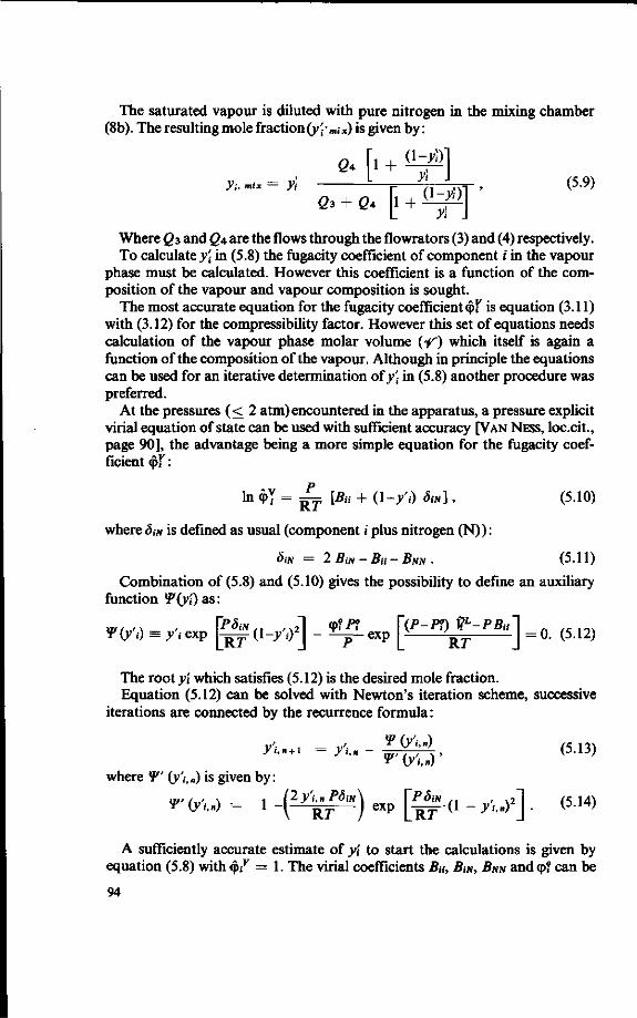
The saturated vapour is diluted with pure nitrogen in the mixing chamber (8b). The resulting mole fraction (yj'm,x) is given by:

Q< [i + <m

Where Q3 and Q* are the flows through the flowrators (3) and (4) respectively. To calculate y\ in (5.8) the fugacity coefficient of component i in the vapour

phase must be calculated. However this coefficient is a function of the com­position of the vapour and vapour composition is sought.

The most accurate equation for the fugacity coefficient q>Y is equation (3.11) with (3.12) for the compressibility factor. However this set of equations needs calculation of the vapour phase molar volume (f) which itself is again a function of the composition of the vapour. Although in principle the equations can be used for an iterative determination of y\ in (5.8) another procedure was preferred.

At the pressures (< 2 atm)encountered in the apparatus, a pressure explicit virial equation of state can be used with sufficient accuracy [VAN NESS, loc.cit., page 90], the advantage being a more simple equation for the fugacity coef­ficient <j>r:

In q>T = ^ [Bu + (1- / , ) 8m], (5.10)

where SIN is defined as usual (component i plus nitrogen (N)):

dm = 2BiN-Bu-BNN. (5.11)

Combination of (5.8) and (5.10) gives the possibility to define an auxiliary function ¥(yt) as:

V(y,) = yt exp J - ^ - (l-y ,)2J - ~ - exp ^ ^ J = 0. (5.12)

The root y\ which satisfies (5.12) is the desired mole fraction. Equation (5.12) can be solved with Newton's iteration scheme, successive

iterations are connected by the recurrence formula:

y'-+1 =yi--wwj>> (5-,3)

where ¥' (y'i,*) is given by:

*" (y>.n) = 1 - ( ^ ^ ) exp [ ^ ( 1 - y'unf] . (5-14)

A sufficiently accurate estimate of y\ to start the calculations is given by equation (5.8) with §? = 1. The virial coefficients Bu, BIN, BNN and q>? can be

94

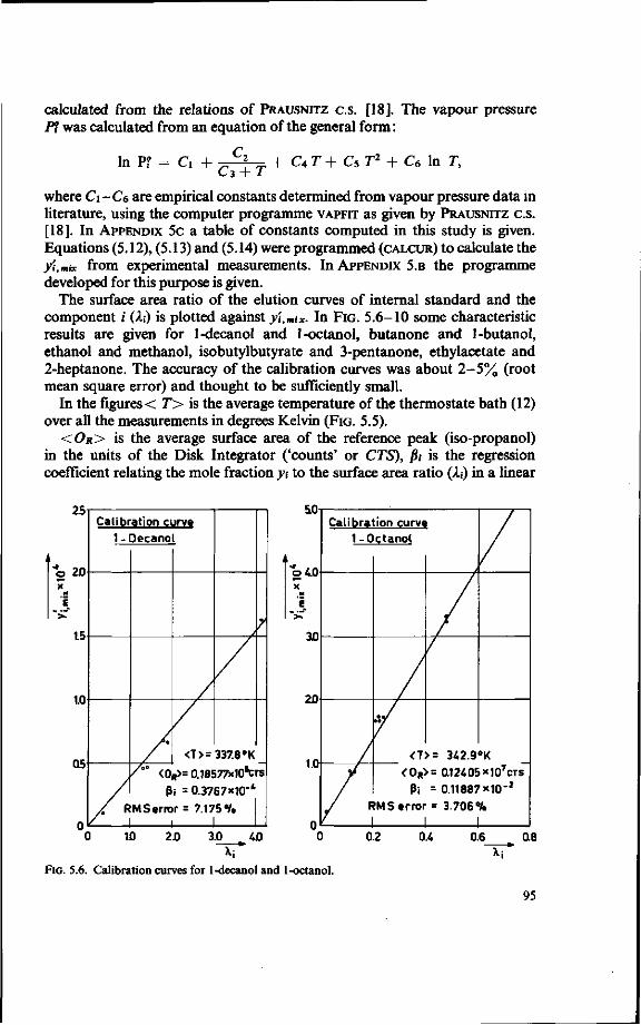
calculated from the relations of PRAUSNITZ C.S. [18]. The vapour pressure P? was calculated from an equation of the general form:

In Pf = d + T T - ^ + CA. T + Cs T2 + C6 In T,

where Ci-Cs are empirical constants determined from vapour pressure data in literature, using the computer programme VAPFIT as given by PRAUSNITZ C.S.

[18]. In APPENDIX 5C a table of constants computed in this study is given. Equations (5.12), (5.13) and (5.14) were programmed (CALCUR) to calculate the y'i.mix from experimental measurements. In APPENDIX 5.B the programme developed for this purpose is given.

The surface area ratio of the elution curves of internal standard and the component i (Xi) is plotted against y'i,miX. In FIG. 5.6-10 some characteristic results are given for 1-decanol and 1-octanol, butanone and 1-butanol, ethanol and methanol, isobutylbutyrate and 3-pentanone, ethylacetate and 2-heptanone. The accuracy of the calibration curves was about 2 - 5 % (root mean square error) and thought to be sufficiently small.

In the figures < T> is the average temperature of the thermostate bath (12) over all the measurements in degrees Kelvin (FIG. 5.5).

<OR> is the average surface area of the reference peak (iso-propanol) in the units of the Disk Integrator ('counts' or CTS), /?,• is the regression coefficient relating the mole fraction yt to the surface area ratio (A,) in a linear

25

2J0

1.5

1.0

05

Calibration curve 1 -

/ R

Decano

A 0

/ <0 p

MSerrc 1

I

<T> =

R>= 0.185 i = 0.37 r = 7.17

337.8 °K

77x10^

67x10"*

5%

rs

10 2.0 3.0 40

FIG. 5.6. Calibration curves for 1-decanol and 1-octanol.

95

1.20

7 100

FIG. 5.7. Calibration curves for 1-butanol and butanone.

1.00 1.00r

FIG. 5.8. Calibration curves for ethanol and methanol.

96

<0R> = O39955xi0*cis

3i =0.30912x10"*

RMS error = 4.0351 °/o

30

FIG. 5.9. Calibration curves for isobutylbutyrate and 3-pentanone.

Calibration curve 2-Heptanone

FIG. 5.10. Calibration curves for ethylacetate and 2-heptanone.

97

equation yi = /Mi. The root mean square error (RMS-error) is defined as the square root from the quotient of the sum of squares of deviations between experimental vs. calculated yi and the number of measurements minus one.

The largest error appears in the calibration curve of 1-decanol; partly this can be explained from the lack of vapour pressure data of this compound at ambient temperature.

5.2.4. The vapour liquid equilibration apparatus

The cylindrical vessel (length 60 cm, diameter 14 cm) used as an equili­bration chamber is sketched in FIG. 5.11. The vessel (1) is provided with a water mantle (2) and a stirrer at the bottom (3). A smaller tank (4), fitting closely inside the vessel, was inserted and sealed at the top by means of an 0-ring. The volume of this tank is about 2000 cm3 smaller than half the volume of the vessel. At its bottom the tank was supplied with a tube (5) reaching almost to the bottom of the vessel. A lid, sealed (6) with an 0-ring, closed the apparatus air tight. A thermocouple (7) and a mercury manometer (8) were used to measure temperature and pressure inside the vessel. The vessel was connected with the nitrogen supply (9) and the sample loop (10), both tubes were supplied with Becker needle valves (11). At the bottom of the vessel a drain pipe with a valve (12) was mounted. At (13) the vessel could be connected with a vacuum pump.

(13) vacuum

-®

<2>

^Ks) <§>

Liquid tevel when up­per compartiment is filled.

<£> Thermostate

FIG. 5.11. Schematic sketch of the vapour-liquid equilibration apparatus for static measurements.

98

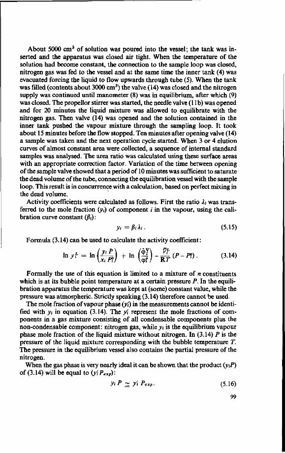
About 5000 cm3 of solution was poured into the vessel; the tank was in­serted and the apparatus was closed air tight. When the temperature of the solution had become constant, the connection to the sample loop was closed, nitrogen gas was fed to the vessel and at the same time the inner tank (4) was evacuated forcing the liquid to flow upwards through tube (5). When the tank was filled (contents about 3000 cm3) the valve (14) was closed and the nitrogen supply was continued until manometer (8) was in equilibrium, after which (9) was closed. The propellor stirrer was started, the needle valve (1 lb) was opened and for 20 minutes the liquid mixture was allowed to equilibrate with the nitrogen gas. Then valve (14) was opened and the solution contained in the inner tank pushed the vapour mixture through the sampling loop. It took about 15 minutes before the flow stopped. Ten minutes after opening valve (14) a sample was taken and the next operation cycle started. When 3 or 4 elution curves of almost constant area were collected, a sequence of internal standard samples was analysed. The area ratio was calculated using these surface areas with an appropriate correction factor. Variation of the time between opening of the sample valve showed that a period of 10 minutes was sufficient to saturate the dead volume of the tube, connecting the equilibration vessel with the sample loop. This result is in concurrence with a calculation, based on perfect mixing in the dead volume.

Activity coefficients were calculated as follows. First the ratio ki was trans­ferred to the mole fraction (yi) of component i in the vapour, using the cali­bration curve constant (fit):

yi=fiikt. (5.15)

Formula (3.14) can be used to calculate the activity coefficient:

*>f-*(£*)+ *$)-&"-">• (314)

Formally the use of this equation is limited to a mixture of n constituents which is at its bubble point temperature at a certain pressure P. In the equili­bration apparatus the temperature was kept at (some) constant value, while the pressure was atmospheric. Strictly speaking (3.14) therefore cannot be used.

The mole fraction of vapour phase (yi) in the measurements cannot be identi­fied with yi in equation (3.14). The yi represent the mole fractions of com­ponents in a gas mixture consisting of all condensable components plus the non-condensable component: nitrogen gas, while yi is the equilibrium vapour phase mole fraction of the liquid mixture without nitrogen. In (3.14) P is the pressure of the liquid mixture corresponding with the bubble temperature T. The pressure in the equilibrium vessel also contains the partial pressure of the nitrogen.

When the gas phase is very nearly ideal it can be shown that the product (yiP) of (3.14) will be equal to (yiPeXp)'-

ytP^y'tPexp. (5.16)

99

A consequence of this assumption also is that the second term of the RHS in equation (3.14) vanishes. If one imagines a system of n constituents at the pressure P (bubble pressure) to be compressed isothermally to a pressure Pexp, leaving the composition unchanged, changes in the values of activity coefficients ( Alnyf, i = l,n) are given by:

As before the assumption that the mixture is remote from its critical con­ditions warrants neglection of differences between V\ and V\, the latter moreover being independent of pressure.

Now (3.14) can be written, by combination with (5.16) and (5.17), in the following form:

This formula was used as a working equation to evaluate In yf from experi­ments. The temperature was measured with the thermocouple (7) in fig. 5.11. The pressure was atmospheric pressure corrected with the readings of mano­meter (8). The liquid mole fraction xi was determined from the Antoine type of equation given by PRAUSNITZ [18], see APPENDIX 5.C.

The molar volume Pf1 was calculated from data on densities at different temperatures using a power series:

Vh= CVi + CV2 T + C'v3 T2 . (5.19)

In APPENDIX 5.c a table with data used in (5.19) is given, the programme INPUT (PRAUSNITZ C.S. [18]) indicates the way Cm, Cy2, and C^3 can be calculated from these data.

5.3. EXPERIMENTAL RESULTS

5.3.1. Introduction

Two series of experiments were carried out. The first series was intended to test the equilibrium apparatus on reproducibility and accuracy. Binary systems were used; the activity coefficients were measured at different con­centrations.

In a second series of experiments multicomponent systems were analysed. In this series the concentration of one of the organic components was increased, while the concentrations of the other components were kept at a low level. The object of these measurements was to determine at which concentration ratios deviation in the activity coefficient values appeared, as compared with those at infinite dilution. Quantitative data in this field are of importance for the design of distillation columns while practically no experimental data are

100

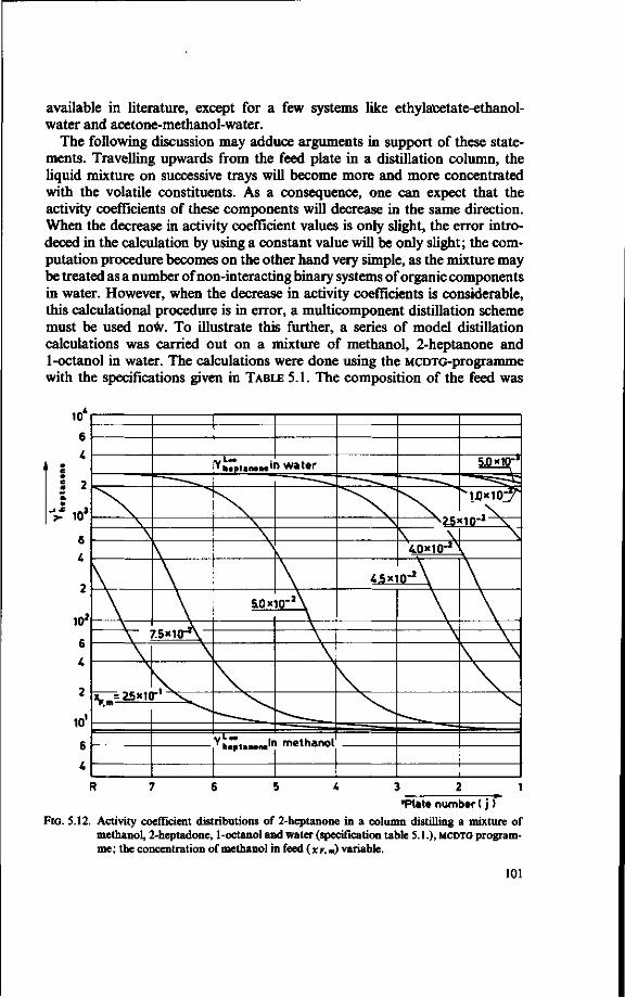
available in literature, except for a few systems like ethylatetate-ethanol-water and acetone-methanol-water.

The following discussion may adduce arguments in support of these state­ments. Travelling upwards from the feed plate in a distillation column, the liquid mixture on successive trays will become more and more concentrated with the volatile constituents. As a consequence, one can expect that the activity coefficients of these components will decrease in the same direction. When the decrease in activity coefficient values is only slight, the error intro-deced in the calculation by using a constant value will be only slight; the com­putation procedure becomes on the other hand very simple, as the mixture may be treated as a number of non-interacting binary systems of organic components in water. However, when the decrease in activity coefficients is considerable, this calculational procedure is in error, a multicomponent distillation scheme must be used now. To illustrate this further, a series of model distillation calculations was carried out on a mixture of methanol, 2-heptanone and 1-octanol in water. The calculations were done using the MCDTG-programme with the specifications given in TABLE 5.1. The composition of the feed was

10*

6

i

5 2

J> 10»

6 i

10J

6

4

10'

6

4

" "^^^

\ 7 . 5 *10 - \

V.nr 2 5*" r x .

virPui»nc'n water

5.0*10_ 2 \

Y i " . In methanol

— - ~ » _ ^

5.0*10-*

\ \ , ^uoxio-?"

^ Z 5 * 1 0 - a X \ \

40*10"^

45x10-* \

1 <Plat« number t j )

FIG. 5.12. Activity coefficient distributions of 2-heptanone in a column distilling a mixture of methanol, 2-heptadone, 1-octanol and water (specification table 5.1.), MCDTG program­me; the concentration of methanol in feed (xr.«) variable.

101

varied in the following way. Leaving the 2-heptanone and 1-octanol concen­tration constant, at a very low level of 0.1 x 10"5 mole fraction, the con­centration of methanol in the feed (xF.m) was increased from 0.1 x 10~5 ->-0.250 in 15 successive steps. In FIG. 5.12 the activity coefficients calculated by SUBROUTINE ACT used in MCDTG are plotted against the index of the plates starting at the reboiler.

It is clearly demonstrated that for a feed concentration of methanol smaller than 0.1 x 10"2 the activity coefficient for 2-heptanone is constant over the whole column while for higher concentrations, or, what amounts to the same in this respect, a longer rectifying section, the deviations become appreciable. The composition ratios between methanol and 2-heptanone are such, that it is not likely that azeotrope formation will interfere with the calculations.

TABLE 5.1. Specification of the distillation example.

F = 100 . moles/sec Activity coeff. equation: VAN LAAR D = 5. moles/sec R = 0.994 (L/V) Rex,= 165.67 (LID) q = 0. (saturated vapour feed) Number of plates = 8 Feed plate location = 4 Pressure =1 .0 (a tm)

In this specific example the multicomponent distillation scheme becomes mandatory at methanol-concentrations of more than 0.1%. When a higher concentration factor (F/D) is specified or when the rectifying section is longer this percentage becomes even lower. In the next two sections the measurements on binary systems (5.3.2) and multicomponent systems (5.3.3) will be discussed.

5.3.2. Measurements on binary systems

The apparatus was tested by measurements of activity coefficients in two homologeous series: normal aliphatic alcoholes and 2-ketones.

Measurements included methanol, ethanol, 1-butanol, 1-hexanol, 1-octanol, 1-decanol, acetone, butanone-2, pentanone-2, pentanone-3, and heptanone-2, all components in water at different concentrations and some systems also at different temperatures.

The calculation of yk from experiments was discussed in section (5.2.4). In FIG. 5.13-5.19 some of the results are given in graphs relating yf to xt. In every figure comparison of the measured values for the acitivty coefficients with values calculated from the solubility limits is made.

The solubility data were obtained from STEPHEN AND STEPHEN [75], LANDOLT-BORNSTEIN [82] and INTERNATIONAL CRITICAL TABLES [60]. The van

Laar constants were calculated from the formulae of CARLSON AND COLBURN,

[14]. Although the temperatures at which measurements were made do not

always match, the conclusion is that solubility data give only a rough estimate

102

10' 8 6

10' 8

6

1

_Solubi

i ,

i t y ( 565

-

'K J—1 r— •

~^ » —*a> r^Z

— -

1 - Butanol + water Legenda

A Data Perry [13] datm.) A Pierotti, Deal, Derr. [39] 4- Burnett [73l(300*K) o Present study (300°K>

Xj *

10" 6 8 10 -4 6 8 W 2 A 6 8

FIG. S.13. Activity coefficient of 1-butanol in a dilute aqueous solution as a function of concen­tration.

• u 8

6

^

2

in2

8

6

U

2

in'

«fr |

- 4 -I

. . 1 1 j) 11

Prom sotuhilitv 7-Haxarml O m ° K ) -<

- i — >•

| 3tfc

" 1

' 0

A

A .

-Hexanol + Water Legenda

Measurements(318°K) Measurements (337°K)

X|

\0~ 6 8 10" 6 8 10' 6 8

FIG. 5.14. Acitivity coefficient of 1-hexanol in a dilute aqueous solution at two temperatures as a function of concentration.

103

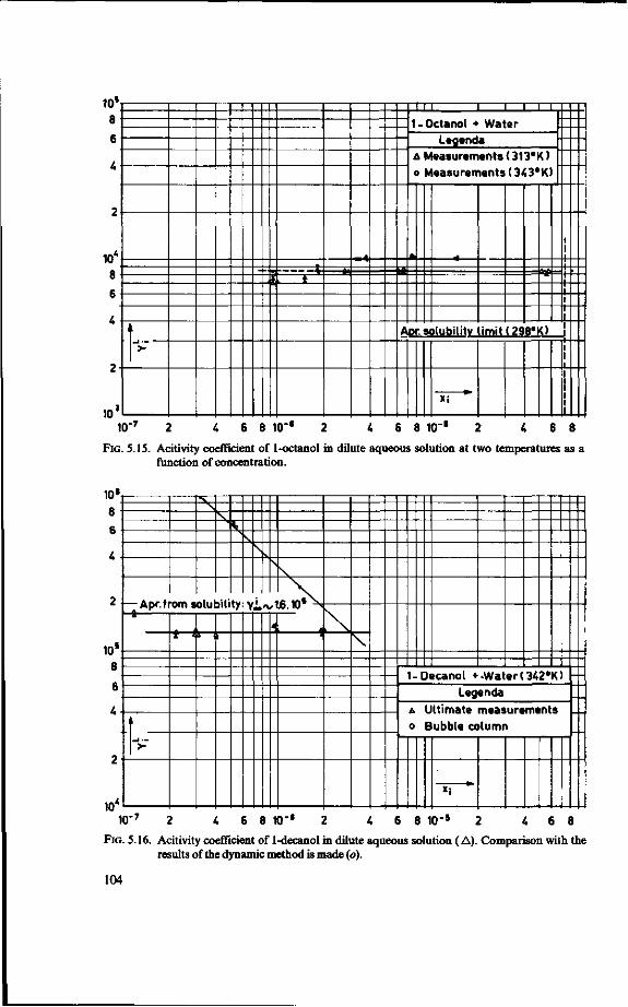
10s

8

6

10*

8

6

10

1

1 I

--._ fc

:t r*i — &

- 1 1

£

0

A

B -

M i 1 i i 1

-Octanol + Water legenda

Measurements (313°K) Measurements (343°K)

** — <-

Aor. solubility limit (298°K) !

Xi 1

10" 4 6 8 10** 4 6 8 irr* 6 8

FIG. S.15. Acitivity coefficient of 1-octanol in dilute aqueous solution at two temperatures as a function of concentration.

10»

8

6

10* 8

6

4

10*

9.

A

_ i . . .

£ * 1 ,

Lege n da

A Ultimate measurements o Bubble column

"i '

10" 6 8 10"6 ! 4 6 8 10"» 2 4 6 8

FIG. 5.16. Acitivity coefficient of 1-decanol in dilute aqueous solution (A). Comparison with the results of the dynamic method is made (o).

104

10!

10' 8

6

Y!"~= 29.392 (363°K) solubility data

>r .-

> '

1

>-

" * -

1

™ » ..£ t o

Butanone + Water Legenda

A Measurements(316*K) o Measurements (295"K)

«•• '

KT 4 6 8 10"* 4 6 8 10"' 6 8

FIG. S.17. Activity coefficients of butanone in dilute aqueous solution at two temperatures i function of concentration.

10J

8 6

10' 8 6

10'

y\~= 1.111 10J f

A

roi n so

r —*-

lubility (30 3"K)

+ -1 • " ~ ^ S a " J ,___.

Pentanone-3 + Water Legenda

•y- Bubble column (305°K) A Static method (293aK) o Static method (316°K)

— i —

^ X|

| I

10 I -7 6 8 10" 6 8 10" 6 8

FIG. 5.18. Activity coefficients of pentanone-3 in dilute aqueous solution (A, o). Comparison is made with results of the dynamic method (^) .

105

IU 8 6

2

io3

A

6

2

m2

jti H 4fL.

Y|-~= 1.481.10' from solubility (303°K)

. - Heptanone- 2 + Water Legenda

A Measurements (326.6*K1

X | "

10" 6 8 10" 6 8 10" 6 8

FIG. 5.19. Activity coefficients of heptanone-2 in dilute aqueous solution as a function of concen­tration.

of the Van Laar parameters. A list of calculated values is given in TABLE 5.2. The influence of the mole fraction xt on the activity coefficients is very slight in the concentration range xt < 10"3, which is, of course, to be expected from thermodynamical reasoning. The accuracy of the measurements is reasonable, although in evaluating the accuracy from the graphs one should note the logarithmic scales on abscissa and ordinate.

It is rather interesting to compare activity coefficients of the two homologeous series (n-alcoholes and 2-ketones) with the PIEROTTI-DEAL-DERR correlations for these series (FIG. 5.20 and 5.21). The results for the n-alcoholes especially are very close to the predicted activity coefficients from the correlations. Again comparison is hampered somewhat by the virtual absence of experimental data on the partial molar heat of mixing (compare equation 3.80) of the higher homologues in water.

It was concluded that the apparatus gives reproducible results. In the course of the investigations also esters (ethylacetate, isobutylbutyrate) and aldehydes (octanal, decanal) were used, however only in multicomponent systems. The values for lnyf at infinite dilution were in agreement with the respective PIEROTTI-DEAL-DERR correlations.

5.3.3. Measurements on multicomponent mixtures

The main object of the experimental part of the present study was to obtain information about mutual interactions of constituents in a multicomponent

106

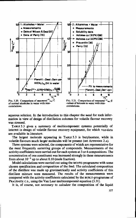
50|-1 - Alcoholes « Water -A Measurements e- Data of Wilson & Deal [A1]/ • Data of Perry [13]

Pierotti - Deal - Derr core

H(CH2)n,OH in water

«»logYh,=-a755+a683ni • •2# f i

-I 1 1- 1! 8 10

au

40 1

£ "" in

0

-2-A(kanones • W. | o Measurements • Solubility data + Hofsteecs(313*K)[69]

o- Hofsteec.s(333°K)[69] a Prausnitz [18] A Perry [13]

i 11

¥ i i

// t V

/...

/ / ! r ' I

— Fit to measurements Pierotti-Deal-Derr corr.

.1 1 1... 1 .

n.-FIG. 5.20. Comparison of measured 10i»»yi of normal alcoholes in water with PDD-correlations.

8 10

FIG. 5.21. Comparison of measured 10i„, -ft -values of ketones in water with PDD-correlations.

aqueous solution. In the introduction to this chapter the need for such infor­mation in view of design of distillation columns for volatile flavour recovery was stressed.

TABLE 5.3 gives a summary of multicomponent systems potentially of interest in design of volatile flavour recovery equipment, for which VLE-data are available in literature.

The largest molecule appearing in TABLE 5.3 is butylacetate, while in volatile flavours much larger molecules will be present (see APPENDIX 2.A).

Three systems were selected, the components of which are representative for the most frequently occurring groups of compounds. Measurements of the activity coefficients were carried out for each system at 3 or 4 compositions. The concentration of one constituent was increased strongly in these measurements from about 10"3 up to about 0.10 (mole fraction).

Model calculations were carried out using the MCDTG programme with some chosen specification and composition of the feed. The calculated composition of the distillate was made up gravimetrically and activity coefficients of this distillate mixture were measured. The results of the measurements were compared with the activity coefficients calculated by the BUBLT-programme of PRAUSNITZ C.S., using the Van Laar multicomponent equation (3.31).

It is, of course, not necessary to calculate the composition of the liquid

107

TABLE 5.2. Van Laar constants from solubility data [Stephen & Stephen, 75], (programme: SOLFIT)

Component in water:

Van Laar constants:

T

303. 363. 293. 303. 333. 373. 293. 303. 303. 303. 313. 365. 293. 303. 293. 303. 273. 288. 293. 313. 323.

^ 1 2

(Inyf")

3.1401 3.3807 4.6001 4.7103 5.0282 4.8045 5.7352 5.8523 7.3008 3.9731 4.0329 3.8855 5.7505 5.8965 4.6134 4.8200 3.9803 4.1942 4.2865 4.3477 4.4734

An Onyi")

1.7647 1.4277 2.9633 2.7614 2.1359 1.6859 2.4602 2.3685 2.5877 1.0741 1.0369 0.8057 1.5409 1.5035 1.2773 1.2724 2.6169 2.3741 2.2399 2.2111 2.0373

butanone

pentanone-3

hexanone-2

heptanone-2 1-butanol

2-hexanol

3-methyl 3-pentanol

ethylacetate

TABLE 5.3. Multicomponent systems containing water and volatile organic compounds [HALA C.S., 83] for which literature data are available.

System Reference

GRISWOLD, BUFORD (1949), [85]

PICK, FRIED, HALA, VILIM (1955), [86]

CARLSON, SMITH, MORELL (1954), [87]*)

BOGNAUGURI, CARPANI, DALL'ORTO (1956), [88]

GRISWOLD, CHU, WINDSAUR (1949), [89]

CARLSON, SMITH, MORELL (1954), [87]

SAMANDAR, NANDI (1948), [90]

JANECKE(1950), [91]

GRISWOLD, DIMVIDDIE (1942), [92]

CARLSON, SMITH, MORELL (1954), [87]

idem

* The data of CARLSON only give relative volatility ratios between the components.

108

water + acetic acid + ethylacetate water + acetone + butanone water + acetone + methanol water + 1-butylacetate + 1-butanol water + 2-butanol + ethanol water + ethanol + acetic acid water + ethanol + ethylacetate water + ethanol + 1-propanol water + ethanol + sucrose water + methanol + isobutanol water + methanol + ethanol water + ethanol + sec-butanol + 1-propanol water + ethanol + 1-propanol + isopropanol

mixture to obtain an impression of the usefulness of the Van Laar multicom-ponent equation. It is however illustrative to choose a composition that could possibly occur in the top of a column, where the largest deviations in activity coefficients from the infinite dilution values appear.

The systems selected are given in TABLE 5.4.

TABLE 5.4. Multicomponent systems used for measurements.

Mixture Components

I methanol, 2-heptanone, 1-octanol, water II ethanol, 1-octanol, 1-decanol, water

III acetone, 1-butanol, isobutylbutyrate, 1-octanol, water

Most measurements were carried out with system I. Four compositions were first calculated with the MCDTG programme and checked experimentally. In addition a number of measurements with mixture I, in which only the methanol concentration was varied, was executed.

The results of the measurements are reduced to tables (TABLE 5.5.1,5.5.II and 5.5.III) and one graph, FIG. 5.22, summarizing the measurements on system I when only the methanol concentration was changed. In the calculations with the BUBLT programme data on critical temperatures, pressures and volumes, acentric factors (co), acentric factors of homomorphs (<wH), dipoles Qi), association factors (>;), constants for a vapour pressure-temperature equation and temperature dependence of the liquid molar volumes were used. Such data can be found in PRAUSNITZ [18], O'CONNELL and PRAUSNITZ [23], for some components and in APPENDIX 5.C for other components.

Data on the Van Laar binary constants were obtained from the experiments on binary systems (section 5.3.2) and literature which was as complete as possible. However no data were available for the binary systems 1-octanol + 1-decanol, acetone + isobutylbutyrate, acetone + octanal, 1-butanol + octanal and isobutylbutyrate + octanal. Except for the systems acetone + isobutylbutyrate and acetone + octanal in mixture III this lack of data is not important because the mole fractions of the components in the multicomponent mixture are both very low. In system III however, the acetone concentration is substantial in some measurements, resulting in large deviations between measured and calculated activity coefficients. The interaction parameters were most frequently obtained from Pierotti-Deal-Derr correlations and from Wilson-Deal formulae (section 3.4).

The results for mixture I show that the calculated yf are fairly accurate ( ~ 5%) at the two most diluted compositions. When the mole fraction of ethanol exceeds 0.017 accuracy decreases, the 2-heptanone activity coefficient especially being badly predicted. This phenomenon can be partly explained through inaccuracy of the interaction parameters for the methanol - 2-heptanone mixture as used in the bubble temperature calculations. Mostly the activity coefficient for methanol ($) me is somewhat lower than the calculated

109

- a

o

I i M

1

s

f

j

1 J I

:

* i -

i

E

•fa

/

i

! >

t

<

*n '

l

1 | L 4*

*

f l

Jl

c c c »—« a I

i CM

«a

i<i

o <

o

^ / / ? /

1 1 I., <

n O

>» > u

•o

• 3

. E o u

o c

: K

- s o o

O

coef

fici

ents

wit

h e

xper

imen

tal

valu

es. A

t P

- 1.0

atm

. V

an

Laa

r eq

uat

ion

s.

o =

Met

han

ol

A =

2-H

ep

tan

on

e

D

= i

- Oct

ano

l

o

JK

i

c

o

o c

o

„

"' 1 \

W i cb

> £ r

E — K -—

J

i

0

J

3 2

;

)

" o

FIG. 5.22. Acitivity coefficients of methanol, methylpentylketone, 1-octanol and water in a mixture as a function of methanol concentrations. Comparison of experimental values with results from BUBLT-programme.

110

value. This deviation may be due to the well-known fact that a methanol peak in a gaschromatogram has a pronounced tendency to 'tail', which can result in too low values for the peak area. Concentrations of methanol higher than 0.123 mole fraction could not be achieved with the experimental apparatus as it was used.

Even at this concentration level the tailing of the methanol peak became so excessive that the 1-octanol and 1-decanol peaks were no longer separated from the methanol peak.

The vapour phase molar volume {'Vmtx) of the mixture increases as the bubble temperature (7») increases, the second virial coefficient of the mixture (Bmix) becomes more negative when 7» decreases. The fugacity coefficients (<pD for the four compositions in TABLE 5.5.1 are given in TABLE 5.6.

TABLE 5.5.1. Measurements of the system methanol + 2-heptanone + 1-octanol + water(r=323.0°K)

Xi

7V») CK)

fmix

(cm3/mole) (cm3/mole) (T^L***) (rf)-?)

1 2 3 4

1 2 3 4

1 2 3 4

1 2 3 4

0.1539 x 10~2

0.3110 xlO"6

0.1687 x 10"' 0.9984

0.3109 x 10-2

0.6157 X 10-' 0.9054 x 10-' 0.9968

0.1689 x 10-1

0 7850 x 10"' 0.1186x10-' 0.9831

0.1229 0.1112x10^ 0.1002 X 10"* 0.8771

372.89

372.65

370.70

360.27

30087.0

30063.0

29869.3

28826.0

-502.4

-506.4

-539.3

-718.1

1.901 2.583 x 103

9.159 x 103

1.000

1.896 2.538 x 103

8.988 x 103

1.000

1.860 2.180 x 103

7.63 x 103

1.000

1.618 7.346 x 102

2.402 x 103

1.010

1.82 2.45 X 103

8.69 X 103

-

1.99 2.46 x 103

8.47 x 103

-

1.70 1.95 x 103

6.7 xlO3

-

1.50 5.77 x 102

2.33 x 103

-

4.25 5.07 5.12

-

4.96 3.07 5.76

-

9.14 10.55 12.19

-

7.30 21.4 2.99 _

*) The (-fi) me are averages of 3 measurements. **) Calculated for P = 1.0 atm.

***) Interaction Parameters:

System

1-2 1-3 1-4 2-3 2-4 3-4

lnrf"

1.336 1.229 0.6447 0.603 7.874 9.141

lnyi"

2.140 4.193 0.5756 1.414 1.421 1.451

Data from:

P75.D-correlations Wilson-Deal formulae Perry, Hdla PDD-correlations Binary meas., PDD-con. Binary meas., PDD-con.

Ill

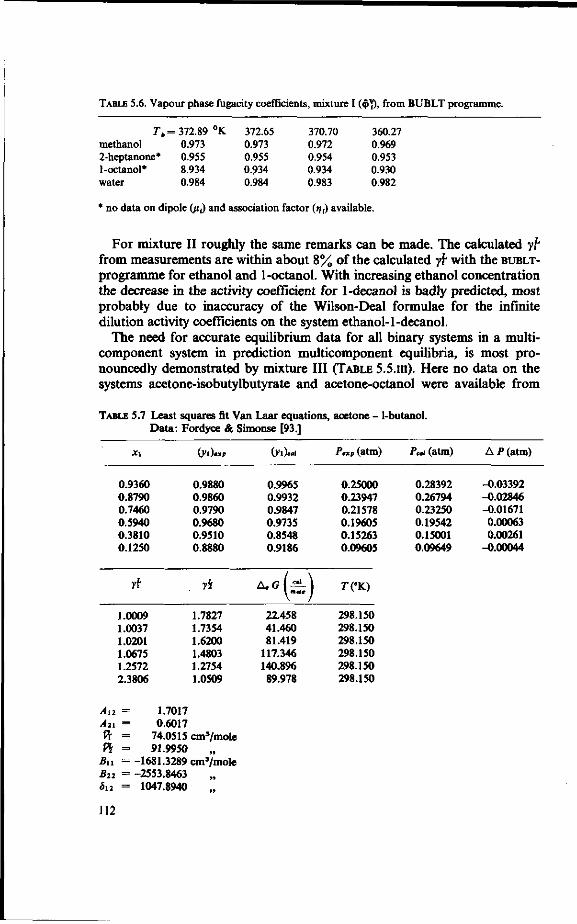
TABLE 5.6. Vapour phase fugacity coefficients, mixture I ($Y), from BUBLT programme.

Tb = methanol 2-heptanone* 1-octanol* water

= 372.89 °K 0.973 0.955 8.934 0.984

372.65 0.973 0.955 0.934 0.984

370.70 0.972 0.954 0.934 0.983

360.27 0.969 0.953 0.930 0.982

* no data on dipole (jit) and association factor (f/() available.

For mixture II roughly the same remarks can be made. The calculated yh from measurements are within about 8% of the calculated yf with the BUBLT-

programme for ethanol and 1-octanol. With increasing ethanol concentration the decrease in the activity coefficient for 1-decanol is badly predicted, most probably due to inaccuracy of the Wilson-Deal formulae for the infinite dilution activity coefficients on the system ethanol-1-decanol.

The need for accurate equilibrium data for all binary systems in a multi-component system in prediction multicomponent equilibria, is most pro­nouncedly demonstrated by mixture III (TABLE 5.5.III). Here no data on the systems acetone-isobutylbutyrate and acetone-octanol were available from

TABLE 5.7 Least squares fit Van Laar equations, acetone - 1-butanol. Data: Fordyce & Simonse [93.]

Xl (yi)e. CFi)" »(atm) Pcai (atm) A P (atm)

0.9360 0.8790 0.7460 0.5940 0.3810 0.1250

0.9880 0.9860 0.9790 0.9680 0.9510 0.8880

0.9965 0.9932 0.9847 0.9735 0.8548 0.9186

0.25000 0.23947 0.21578 0.19605 0.15263 0.09605

0.28392 0.26794 0.23250 0.19542 0.15001 0.09649

-0.03392 -0.02846 -0.01671 0.00063 0.00261

-0.00044

yt yi AeG \ more I r(°K)

1.0009 1.7827 1.0037 1.7354 1.0201 1.6200 1.0675 1.4803 1.2572 1.2754 2.3806 1.0509

Ai2 = 1.7017 An = 0.6017 % = 74.0515 cm3/mole Pi = 91.9950

Bn = -1681.3289 cm'/mole B22 = -2553.8463 «5u = 1047.8940

22.458 41.460 81.419

117.346 140.896 89.978

298.150 298.150 298.150 298.150 298.150 298.150

112

TABLE 5.5.II. Measurements of the system ethanol + 1-octanol -f 1-decanol + water (T= 338.0 °K)

i

1 2 3 4

1 2 3 4

1 2 3 4

Xi

0.3049 x 10-' 0.5350 x 10-7

0.2834 x 10-7

0.9996

0.7645 x 10-2

0.8374 x 10"' 0.3692 x 10-' 0.9920

0.4188 x 10-1

0.5193 x 10-' 0.4623 x 10-' 0.9581

7V") (•K)

373.05

371.24

365.70

"if »i* (Cm3/mole)

30102.9

29912.0

29355.0

B . mix

(cm'/mole)

-499.8

-540.5

-638.4

(yiW*)

4.369 9.262 x 10' 1.308 x 10' 1.000

4.224 7.781 x 103

1.051 x 10' 1.000

3.656 3.634 x 10' 4.043 x 10* 1.003

(tf)~*)

4.3 8.6 xlO' 1.2 xlO'

4.2 8.0 xllO* 1.16

3.95 3.83 x 10* 3.1 xlO*

| A |

1.58 7.15 8.26

0.57 4.24

10.56

8.04 5.39

23.32

*) The (•/:)** are averages of 3 measurements. ***) Calculated for P = 1.00 atm. ***) Interaction Parameters:

System

1-2 1-3 1-4 2-3 2-4 3-4

Inyi"

1.200 1.630 1.476

-9.141

11.79

In yi"

1.280 1.740 0.967

-1.451 1.450

Data from:

Wilson-Deal formulae Wilson-Deal formulae Perry., FDD correlations no data Binary meas., PDD-corr. Binary meas., PDD-corr.

literature while there are no PDD-correlations for these systems as yet. For an ethanol mole fraction of 0.054 the lack of these data results in a totally wrong value for y[ (third group of data in TABLE 5.5.ni).

When, however, data are available (as was the case in the acetone - 1-butanol system, see TABLE 5.7) the multicomponent activity coefficients equation gives fairly good results, taking into account the accuracy of the data for the acetone - 1-butanol system. It must however be stressed that VLE-data for the binary systems not containing water should preferably be measured with the conventional experimental methods (isoteniscopes, equilibrium stills etc.) as there is no need to measure the equilibria in the dilute regions.

As said before the compositions of the mixtures I, II and III in the TABLES 5.5.1—5.5.IH were calculated using the MCDTG programme. In all the calculations a concentration factor (F/D) of 20 was used. In all the FIG. 5.23-5.25 the con­centration distributions of each component along the distillation column are given for the three mixtures with the highest concentrations of organic com-

113

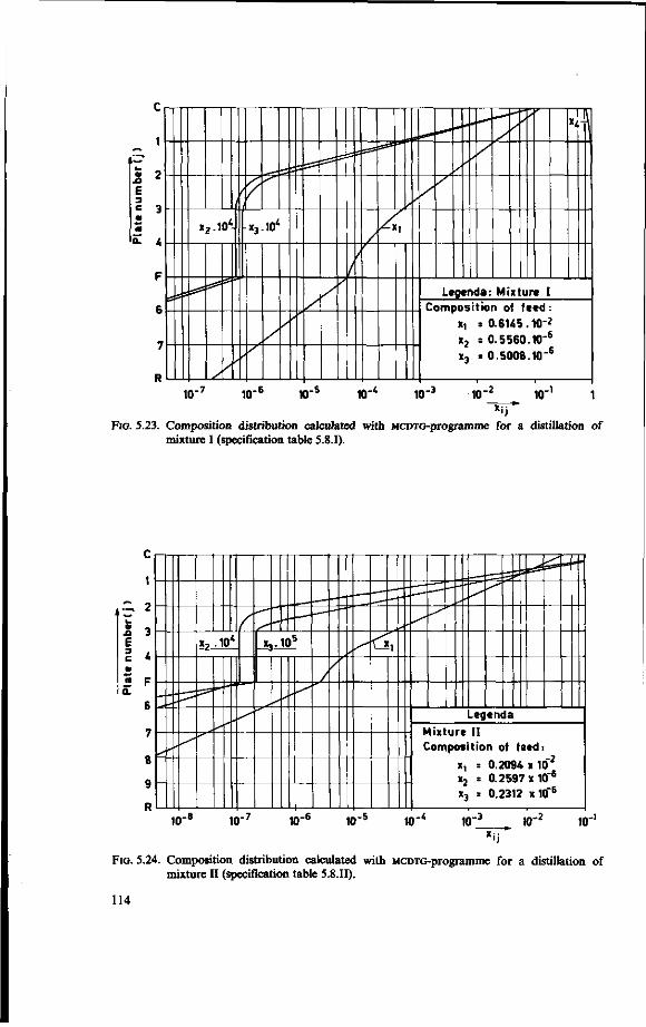
c

1

i * £ 3 <= 3 • a

CL i

*2.10*- x3.10<

/

/ x .

";1

Legend a: Mixture I C

x, = 0.6U5.10"2

x, = 0.5560.10"6

X 3 = 0.5008.10"

1 |

5

10 -7 10" 10 -5 10" 10 -3 10' 10"

FIG. 5.23. Composition distribution calculated with MCDTG-programme for a distillation of mixture I (specification table 5.8.1).

•s 2

1 3 E I 4 2. F a.

6

7

8

9

x2.10 t Xj.lO5

l_

<*y

Legenda f, C fixture I I Composition of feed:

x, = 0.2094 x10~2

x, = 0.2597 xlO"6

> 3 s 0.; !31i » x1 S"6

10 -8 10 -7 10" 10 -5 10' 10" 10 -2 10'

FIG. 5.24. Composition distribution calculated with MCDTG-programme for a distillation of mixture II (specification table 5.8.II).

114

ponents. In TABLE 5.8.i-5.8.m the specifications are given as well as the Kjt, yjt, xji and yft values for the first and second plate (/' = 1,2).

The following important conclusion can be drawn from these figures and tables. Due to the high Kji values differences between the concentrations in the distillate are very large for the organic components. As a consequence activity coefficients on the first plate (yL

a,i = l,n) are those of a solution substantially more diluted than the distillate.

From comparison of e.g. TABLE 5.5.III and 5.8.in it follows that activity coefficients on the first plate in TABLE 5.8.III are comparable with those for the composition on the second plate in TABLE 5.5.m.

TABLE 5.5.IU. Measurements of the system acetone + 1-butanol + isobutylbutyrate + octanol + water ( 7 = 338.0 °K).

Tf*) r „„ "mix I A | i Xi (»K) (cm3/mole) (cm3/mole) ( t fV**) (rf)-.*) <%)

1 0.1060 XlO"3 372.69 30060.3 -512.2 2 0.6730x10-* 3 0.2412X10"5

4 0 .1111x10-* 5 0.9998

1 0.2001 x 10~2 370.16 29795.0 -567.9 2 0.2615x10-* 3 0.1079x10-* 4 0.1063 5 0.9978

1 0.5390X10"1 347.37 27575.7 -897.9 2 0.4094 x lO" 2

3 0.3043 XlO- 5

4 0.4122x10-* 5 0.419

*) The (yh)„e are averages of 3 measurements. **) Calculated for P = 1.00 atm.

***) Interaction Parameters:

10.88 47.80 2.064 x 10* 1.262 1.000

10.73 46.20 1.913 x 10* 1.180x10* 1.000

6.620 22.34 (2.264 X 103) (1.727 X 103) 1.012

9.67 45.2 2.12 X 10* 1.24 X 10*

-

9.23 42.01 1.6 x 10* 0.9 x 10*

-

6.82 20.54 9.8 xlO3

8.5 xlO2

-

11.52 5.49 1.57 2.75

-

4.55 9.07

16.36 23.7

-

3.02 8.06

---

System

1-2 1-3 1-4 1-5 2-3 2-4 2-5 3-4 3-5 4-5

lnyT

1.7010 --

2.392 1.007

-3.868

-9.947 9.545

In yh~

0.6017 --

1.479 0.179

-0.056 1.2664

-1.133 1.325

Data from:

Fordyce & Simonse (see table 5.7) no data no data Perry, binary meas., PDD-COTT. .PZ)D-correlations no datum, PZ)Z)-correlation binary meas., PDD-correlation no data P^D-correlation PvDD-cofrelation

115

O)

c 01

« 3 0.

X , . 1 < > 3 IK

J

_l

o5

/'l

1 -*c_ '2 -X)

-

Legenda

Mixture I I I Composition of feed '•

x, = 0.2695 x 1(T2

x , = 0 . 2 0 i 7 x in" 3

'3 = «4 =

0.15215 0.2061

xlO"6

xKf*

10- io- 10-6 10" 10" 10" 10 -2 io-

FIG. 5.25. Composition distribution calculated with MCDTG-programme for a distillation of mixture HI (specification table 5.8.III).

TABLE 5.8.I. Equilibrium constant and composition distribution on first two plates (Mixture I, MCDTG-programme).

Plate Comp. « (0 Kjt Xjl yji*) yft

1 2 3 4

1 2 3 4

5.77330 0.236327 X 103

0.154986 X 103

0.896196

6.42197 0.323468 X 103

0.219870 X 103

0.981801

0.2128 x 10-' 0.4705 x 10"' 0.6462 x 10-' 0.9787

0.3346 X 10-* 0.2139 x 10-» 0.3844 x 10-9

0.9966

0.1229 0.1112x10"* 0.1001 x 10"* 0.8770

0.2149 x 10-' 0.6920 X 10"' 0.8453 X 10"' 0.9785

1.848 0.2079 X 10* 0.7246 X 10* 1.000

1.986 0.2532 X 10* 0.8963 X 10* 1.000

*) The compositions yu (i= \,n) are equal to the concentrations in the distillate (*DI).

Specification of distillation Composition of feed Comp. (/) Xri

Moles of feed (F) Moles of distillate (Z>) Quality of feed (G) Reflux ratio (L/V) External reflux (L/D) Feed plate location No. of components No. of plates Column pressure (PI)

= 100.0 (moles/sec) = 5.0 (moles/sec) = 0.0 = 0.998 = 499.0 = 5 = 4 = 8 = 1 (atm)

1 2 3 4

0.6145 X lO"2

0.5560 X 10"« 0.5008 X lO"6

0.993854

116

TABLE 5.8.U. Equilibrium constant and composition distribution on first two plates (mixture II, MCDTG-programme).

Plate Comp. (/) ' (0

1 1 2 3 4

2 1 2 3 4

*) The compositions yu

K*

9.18515 0.199206 x 103

0.893876 x 103

0.962518

9.66893 0.230812 X 103

0.106063 X 10* 0.995899

JtJI

0.4559 x 10"2

0.2607 x 10-7

0.5173 x lO"8

0.9954

0.4735 X lO"3

0.1241 X lO"9

0.7054 xlO"11

0.9995

yj<*)

0.4188 x 10"1

0.5194 x lO"5

0.4624 x 10-* 0,9581

0.4578 X lO"2

0.2865 x 10~7

0.7482 x 10-" 0.9954

yh

4.286 0.8379 x 10* 0.1154 XlO6

1.000

4.366 0.9226 x 10* 0.1302 x 10s

1.000

(i = l,n) are equal to the concentrations in the distillate (xn).

Specification of distillation

Moles of feed (F) Moles of distillate (£>) Quality of feed (G) Reflux ratio (L/K) External reflux (L/D) Feed plate location No. of components No. of plates Column pressure (PI)

= 100.0 (moles/sec) = 5.0 (moles/sec) = 1.0 = 0.9995 = 1999.0 = 5 = 4 = 10 = 1 (atm)

Composition of feed Comp. (i) Xn

1 0.2094 x lO"2

3 0.2597 X 10"* 3 0.3212 x 10"« 4 0.9979

For the last mentioned composition fair agreement between calculated and measured activity coefficients was reported above. Similar remarks can be made for the two other distillations, as the reader may infer.

Thus, the composition of the distillate may be such that for calculation of activity coefficients the interactions are by no means negligible, while for the composition on the first plate this neglection is perfectly possible.

However when the Murphree efficiencies are included in the calculations the situation becomes less favourable, because the differences between the XDI and jcii now become smaller.

Summarising the results of the measurements on multicomponent systems one can say that:

(i) The apparatus can be used for simultaneous measurements of infinite dilution activity coefficients of organic components in water;

(ii) The mutual interactions of the organic components in an aqueous solution must always be taken into account when very accurate VLE-calculations are to be made from binary data. When the sum of concentrations of the organic components is less than about 0.02 mole fraction the interactions are negligible in approximate calculations;

117

TABLE 5.8.III. Equilibrium constant and composition distribution on first two plates (mixture III, MCDTG-programme).

Plate (/)

1

2

Comp. (0

1 2 3 4

1 2 3 4 5

Kj<

0.377828 x 10* 0.224428 x 10* 0.297407 x 10' 0.943505

0.400532 x 10* 0.244751 x 10* 0.337509 x 10* 0.152638 x 10' 0.998408

Xji

0.1426 X 10"* 0.1824 X 10"' 0.3248 x 10-7

0.9983

0.3627 x 10~* 0.7533 x 10"' 0.7538 x lO"12

0.2262 x lO"9

0.9999

yji*)

0.5390 X lO"1

0.4094 x 10"* 0.4122 X 10"' 0.9419

0.1452 x 10"* 0.1843 x 10"' 0.2544 x lO"8

0.3453 x 10-7

0.9983

yh

0.1073 X 10* 0.4670 X 10* 0.1196 X 10' 1.000

0.1092x10* 0.4781 X 10* 0.2084 X 10' 0.1273 X 10' 1.000

1 2 3 4 5

0.2695 x 10-* 0.2047 X 10"' 0.15215 x 10-« 0.2061 x 10-6

0.9971

*) The compositions yu(i=l, n) are equal to the concentrations in the distillate (xDi).

Specification of distillation Composition of feed Comp. (i) XFI

Moles of feed (F) = 100.0 (moles/sec) Moles of distillate (D) = 5.0 (moles/sec) Quality of feed (C) 1.0 Reflux ratio (L/K) = 0.9995 External reflux (LID) = 1999.0 Feed plate location = 5 No. of components = 5 No. of plates = 8 Column Pressure (PI) = 1 (atm)

(iii) To the end of distillation calculations the condition mentioned under (ii) can be relaxed in many cases where the components have large Kjt factors because these result in steep concentration gradients in the column. As a rule of thumb it can be stated that when the condition: n - l

Z XD' ~ ( 1 ~Jr'G) yii < 0.02-0.05 (water is n'th component). (5-15) Ku EbG ~

i =1

is met, interactions between organic components can be deleted from the cal­culations without a serious loss of accuracy.

118

6. DISCUSSION AND CONCLUSIONS

In the theoretical part of the study activity coefficients are put forward as the most effective tools to describe the vapour liquid equilibrium relationships needed in design of flavour recovery units. It is remarkable that in literature on volatile flavour recovery problems hardly ever this concept is introduced, while at the same time it is almost impossible to find a paper on vapour liquid equilibria in chemical engineering literature in which the term is not used. As has long been recognized by thermodynamicists, the concept is very useful indeed for description of deviations from ideality and its use should be pro­moted in design of flavour recovery plants. Especially the reduction of vapour liquid equilibrium measurements in two-parameter equations like Van Laar or Enthalpic yl-equations is most effective.

The conclusion on use and measurement of activity coefficients can be summarised as follows:

(i) The framework of thermodynamics of liquid mixtures provides utterly efficient tools to organize vapour liquid equilibrium measurements and to reduce experimental data to a few meaningful parameters. The activity coef­ficients at infinite dilution are related in a simple way to these parameters. Measurements should be limited to binary systems and these experimental data reduced to two parameters per system. For multicomponent VLE de­scription a thermodynamic model should be used, which synthetises the complete behaviour of the systems from a suitable set of parameter pairs. In such a 'scaling up' procedure (an expression due to Prausnitz in this connection) the multicomponent system vapour liquid equilibrium is estimated with reason­able accuracy, limiting experimental work to a minimum.

(ii) Thermodynamic properties of binary systems can be compounded to properties of a multicomponent system. There is a question as to which thermodynamic model is the most effective for the 'scaling up' procedure, needed in prediction of multicomponent VLE. A lattice model of a multicom­ponent solution is discussed. In a general equation for the excess Gibbs free energy function in lattice model parameters (r, z), different definitions of binary system parameters (A, T) lead to different activity coefficient/compsition equations. Moreover either the enthalpy part or the entropy part can be deleted from the excess Gibbs free energy function, which again yields different activity coefficient/composition equations.

From such a lattice model of liquid solutions, a number of two parameter equations for activity coefficients were deduced: the well known Van Laar and Wilson equations and three other equations, the T-equations, yl-equations and Enthalpic .4-equations. For systems showing limited miscibility the Wilson equations cannot be used. In general the T-equations were shown to be inferior to the other equations. The /1-equations give results of comparable accuracy to the Van Laar equations for a number of binary systems. The Enthalpic A-equations in general give better results than the Van Laar equations. An

119

advantage of the Enthalpic yl-equations over the complete /[-equations is their simplicity and, secondly, the comparative ease with which the parameters are estimated from experimental data on infinite dilution activity coefficients.

(iii) Measurement of vapour liquid equilibrium in the miscible region of systems showing a large region of partial miscibility requires special tech­niques. Due to the deviations from ideality in the liquid phase both, liquid phase and gas phase equilibrium composition have to be determined. Such measurements can be done efficiently using a gas chromatographic technique. The method can be used to measure activity coefficients at infinite dilution in water simultaneously for a number of components. Concentration dependence of activity coefficients also can be determined with the apparatus, while, last but not least, measurement of activity coefficients in juices in situ is possible. For aqueous solutions of normal alifatic alcoholes and ketones the proper function­ing of the apparatus was checked.

(iv) The interactions between organic components in an aqueous multi-component solution result in composition dependence of the activity coef­ficients of each constituent. The interactions vanish in the limit when all organic components approach infinite dilution. Data on binary VLE of all organic components in water thus form the minimum information needed, which is sufficient when the sum of concentrations of all organic components is low. In concentration regions where the sum of the organic component mole fractions is (say) some mole percent or more, the interactions are no longer negligible. For three mixtures changes in activity coefficients of the organic components were measured when the concentration of one component was increased (the variable concentration component). Activity coefficients calculated with a multicomponent system Van Laar equation (eqn. 3.31) did match with measured values provided that sufficient data on binary VLE of the variable concentration component with other organic components are available in addition to the data already mentioned.

Once the vapour liquid equilibrium relationschips of a mixture have been established, a distillation column for that mixture can in principle be designed. In the field of volatile flavour recovery ROGER and TURKOT [loc.cit.] were the first to calculate a column with a simple McCabe-Thiele procedure. In the present study design problems of flavour recovery columns were considered and the results can be summarised as follows:

(i) Flavour recovery distillations in essence are multicomponent distillations. Multicomponent distillations can be performed very rapidly with a digital computer. We developed computer programmes (MCDTG and MCDTG-EFF) which are particularly suited to flavour design calculations, as the activity coefficients are included in the equilibrium relation employed in the programme and care is taken for appearance of separated light and heavy components, ^-factors are calculated from the following input data: operating pressure, a set of $n(n-l) binary parameter pairs for the (Van Laar) activity coefficient/ composition equation and finally n sets of 4 constants in a vapour pressure/

120

temperature relation (for 33 components frequently appearing in flavours such constants are calculated in this study). The set of ±n(n-l) binary parameter pairs does not necessarily have to be complete: in the limit when the compo­sition of the distillate is very dilute only n parameter pairs are needed. When the activity coefficient equation is suitably adjusted (ACTINF(MARK)) the number of parameters is futher reduced to n, which is the absolute minimum of infor­mation needed for a particular problem. Some examples are given, (section 4.2 and 4.4), where interactions are negligible; other examples show that inter­actions must be included in calculations. As a rule of thumb, equation 5.15 could be used to make a decision which of the two procedures must be followed in a particular situation.

A typical calculation of a mixture of seven components on a column of ten plates will require less than about .2 minutes on a very large computer, e.g. an IBM 7094. A smaller computer, e.g. an ELX8 needs appr. 0.8 minutes for such a calculation. Block diagrams and FORTRAN listings are given together with a description to make the programmes as easily accessible as possible. In sample calculations the programmes give reliable results.

(ii) Plate efficiencies always have to be taken into account in design of a multicomponent distillation column. This statement was confirmed by the results of calculations for some examples. Especially the distillation of low concentration mixtures reveals this need. The efficiencies are strongly de­pendent on the slope of the equilibrium curve: [m ]. For a binary system:

E%G = 1- exp \-Ujr%-*+ ^k {jf%-i\ (6.1)

A high value for my results in a low efficiency. In flavour distillations very high values for [m] must be anticipated, making calculations of efficiencies practically obligatory.

Theoretically the efficiencies in a multicomponent system have a rather complex relationship to the gas phase and liquid phase transfer resistances, reflux ratio, and the slope of the equilibrium curve, which, in turn is awkwardly related to the thermodynamic properties of the mixture and the column operating variables.

In an analysis a fairly general calculation procedure fo the efficiencies is given. The feasibility of using the complete calculation scheme unfortunately is poor, but it provided guiding lines along which simplifications were established. The assumptions needed in the endeavour to simplify calculations seem to be warranted in many cases.

121

7. A P P E N D I C E S

APPENDIX 2A

Classification of flavour components and composition of flavours for some fruit juices.

In the paper of GIERSCHNER and BAUMANN [12] the components appearing in flavours of apples, pears, cherries, peaches, strawberries, raspberries, black currents, oranges, lemons, grape fruits, lime juice and pineapples range from methane (in oranges) to 4(2,5,6,6-tretramethyl-2-cyclohexen-l-yl)-3-buten-2-on (in strawberries). This may illustrate the diversity and complexity of the flavour components.

Suitable classification of flavour constituents thus becomes a problem on itself, as the criteria giving the most effective classification are not clearly defined, GIERSCHNER and BAUMANN [loc. cit. ].

For the purpose of design of flavour recovery units the classification ROGER and TURKOT [4] give (in which boiling points and water-solubility properties are used as criteria) is useful.

However a better classification of the components probably is just to arrange them in the direction of an increasing relative volatility at infinite dilution with respect to water (tzZ) and/or activity coefficients at infinite dilution in water (yf Z).

The effects of the extent of non-ideality on VLE of a binary mixture of the flavour component in water is expressed in the activity coefficient (compare with solubility criterion of Roger and Turkot). The effect of vapour pressure (compare with boiling point criterion of Roger and Turkot) together with the activity coefficient is reflected in the value of the relative volatility. Thus it appears that the classification of Roger and Turkot can be replaced by using an w. The advantage of the use of the on »is that the classification no longer con­tains 'groups' but only individual components; thus the classification features sharper 'resolution abilities'. One could make a classification as follows:

aZ

I. a," < 1

II. a," > 1

l»rf =

—

0 < In ytz < 2.7

Type of components

strongly polar components (amino-acids, carboxilic acids, etc.)

components are miscible with water in all proportions, positive deviations from ideality (methanol, propanone, ethanone etc.)

III. a-~ > 1 In y,1- > 2.7 components are partially miscible with water, deviations from ideality are strongly positive (butanol, ethylacetate, butanone, methyl-anthranilate etc.)

122

Most of the aroma-components will belong to group III. These components are recovered over the top although their boiling point may be lower than that of a water because the activity coefficients are very high (molecules are very dislike to water molecules, resulting in large deviations from ideality). A large subgroup of group III is the group of heterogeneous azeotrope formers. When the distillate is a one phase mixture, however, this property is not important as the operating line for the top section crosses the diagonal in an (y, x)-diagram left from the miscibility limit. The statement of ROGER and TURKOT that... 'these compounds are probably the most difficult to rectify'... and: 'that these compounds are recovered in the overhead product of a distillation column because they form heterogeneous minimum boiling azeotropes which boil below 100°C at normal conditions...' is not quite correct as the azeotropic composition needs not to be reached to obtain these components in the over­head product.

All components with atZ > 1 can, in principle, be recovered overhead, the higher <Xi w the easier separation will be achieved (less plates are needed).

Now some quantitative data will be given of volatile flavour compositions, taken from DUPAIGNE [11 ].

For pineapple juice the composition of the flavour is given to be (HAAGEN

' ' TABLE 2A. 1. Flavour composition of pineapple juice.

component

ethylacetate acetaldehyde ethanol methylisocaproate methylisovalerate methylvalerate methylcaprylate ethylacrylate ethylcaproate ethylcaproate

es (DIMICK and CORSE):

concentration in winter

2.91 0.62

1.4 0.6 0.49 0.75

TABLE 2A.2. Flavour composition of strawberries.

component

ethanol esters 2-hexenal acetaldehyde methanol acetone 1-caproic acid 1-valeric acid 1-butyric acid acetic acid

concentration in

45.5 9.4 7.2 4.9 4.7 2.7 1.5 0.8 0.5 0.1

mg/kg summer

119.6 1.35

60.5

0.39

0.77 0.77 0.77

p.p.m.

123

WEBB and KEPNER found the following components in Muscat grapes:

TABLE 2A.3. Flavour composition of Muscat grapes.

Component

ethanol methanol 1-butanol 3-methylbutanol 1-hexanol 3 cis-hexanol acetaldehyde hexanal methylethylketone (butanone)

Concentration in mg/kg

methylpropylketone (2-pentanone) 2-hexenal methylacetate ethylcaproate

111. 3.7 0.03 0.01 0.49 0.26 0.85 0.03 0.01 0.01 0.05 0.08 0.04

ROGER and TURKOT [4] estimate the concentration of methylanthranilate in Concord grape juice as 2.37 x 10" 7 mole fraction. An other 'flavour impact' compound appears to be n-butylphtalate in Zinfandel grape juice (HAAGEN

SMIT).

APPENDIX 3.A.

Estimating A-parameters from infinite dilution activity coefficients for the enthalpic A-equations.

In this appendix a FORTRAN programme is given which calculates the ^-para­meters for the enthalpic ^-equations from data on infinite dilution activity coefficients (ENTLAM).

Nomenclature:

ENTLAM Programme title FLAM2 Current estimates of /I21 parameter FL1 Infinite dilution activity coefficient of component 1 In yj'") FL2 Infinite dilution activity coefficient of component 2 In y\ ") V11 Molar volume in liquid phase, component 1 VL2 Molar volume in liquid phase, component 2 T Temperature (°K) PSI Function W defined by equation (3.102) DERIV Derivate of V: W XL12 Final estimate of A12 X L21 Final estimate of A 21 VRAT Ratio of molar volumes ( l£7 ^ ) C21 Interaction energy (A12-A22) C12 Interaction energy (A12 - Au)

124

The programme starts with the reading of a title card followed by a card containing the two infinite dilution activity coefficients, the molar volumes of both components and the temperatures in degrees Kelvin at which these data are valid.

The function *P(A2l) = 0 is then solved using the Newton method. A sui­table initial value for An = 0.5. When convergence is reached the final esti­mates of An, An, W and the number of iterations are printed.

The programme then calculates (A12-A,,)-and (A12-A22) after which it prepares to accept new data for another system.

Read: INPUT FL1,FL2,VL1.VL2.T

FLAM2(1)=0.5

i = 2

i = i + t

Compute:

FLAMli)=FLAM(i-1)--J, Print:

C21.C12.T, VL1.VL2.

Compute: XL12.XL21

Compute: C21.C12

FIG. 3.A-1. Block diagram of the ENTLAM-programme.

125

C PROGRAMME TO OBTAIN ENTHALPIC LAMBDA-PARAMETERS FROM END ACTIVITY C COEFFICIENT DATA C C

DIMENSION FLAM2U00) 9 READ 8

PRINT 8 READ 1. FLl.FL2»VLl»VL2tT H » LOG(FL2/FLl> FLAM2<1)= 0.5 DO <t I« 2<102 PSI« 2 . * L O G ( F L A M 2 U - l ) ) + F L A M 2 I I - 1 X F L 2 • H DERIV « 2 . /FLAM2CI -1 ) + FL2 FLAM2( I )« F L A M 2 I I - H - PS I /DERIV IF(ABS(PSI> - 1.0E-07) 3,3.4

3 XL12 « FLAM2(I»*FL2/FL1 XL21 » FLAM2II) PRINT 5»XL12»XL21»PSI.I 60 TO 6

4 CONTINUE 6 VRAT « VL2/VL1

C21 = (LOG(l./VRAT) - LOG!XL21))*1.98719»T C12 » (LOG«VRAT)-LOG(XH2))*1.98719»T PRINT 7t C12, C21.T . VL1. VL2 GO TO 9

1 FORMATI5F12.6) 5 F0RMAT|3E14.8tI4> 7 F0RMAK2E14.8 , 3F12 .6 ) 8 FORMAT(80H

1 END

APPENDIX 4.A.

Computer programme for multicomponent distillation assuming ideal plates (MCDTG).

A FORTRAN programme is given which calculates a multicomponent distil­lation following the Thiele Geddes calculational procedure*). The programme was made suitable for an IBM-1620 digital computer with a 4QK memory, by dividing it in sub-programmes linked with CALL LiNK-statements. If a computer with a larger storage capacity is used these linkages can of course easily be removed in which case the coMMON-area can be reduced substiantally.

Nomenclature: CACTCO Binary interaction parameter (Ay) CPSAT Constants in vapour pressure equation (Ci-C*) PSAT Pure-component saturation pressure (P?) GAMMA Activity coefficient in liquid phase (yf) T Temperature (°K) PK Equilibrium constant (Ku) ZF Mole fraction in feed (ZFi) GAM Activity coefficient in first iteration cycle (y\) * Some parts of the programme are equal to an EPL-programme of CAPATO [19].

126

XXD YXD XXW YXW XD XW X Y SUMX SUMY F D Q R FT CN TNC PI NC NTC NFT THETA FUNCT DERIV CHECK DELTA EL ELBAR VBAR RBAR MARK

W NH, NL

YHXW

XHXW

YLXD

XLXD

Liquid mole fraction ratio (xJxDi), top section Vapour phase mole fraction ratio (yJxDi), top section Liquid mole fraction ratio {xjxw^, bottom section Vapour phase mole fraction ratio (yt/xWi), bottom section Mole fraction in distillate (xDi) Mole fraction in waste (xWi) Mole fraction in liquid phase (xtj) Mole fraction in vapour phase (ytf) Sum of mole fractions, liquid phase Sum of mole fractions, vapour phase Molar flowrate of feed (moles/sec) Molar flowrate of distillate (moles/sec) Thermal condition of feed Internal reflux ratio in top section (L/V) Location of feed tray Number of components Total number of trays (+ reboiler) Column pressure (P) Fixed point variable, number of components Fixed point variable, total number of trays Fixed point variable, location feed tray Convergence parameter (3-method) Function !P(3), equation (4.16) Derivative ¥" (S) Flag to indicate convergency decision Variable used in convergency decisions Liquid flowrate in top section (L), moles/sec Liquid flowrate in bottom section (L), moles/sec Vapour flowrate in bottom section (V), mole/sec Reflux ratio in bottom section (/?) Flag to communicate to activity coefficient-calculating-SUBROUTINE the first iteration Flowrate of waste product, moles/sec Vectors indicating occurrence of separated light and heavy components respectively Vapour phase mole fraction ratio for a heavy component

\x~wi)

Liquid mole fraction ratio for a heavy component \Xy

Vapour phase mole fraction ratio for a light component

Liquid mole fraction ratio for a light component lx\ \

127

REXT External reflux ratio (L/D) B Reboil ratio (V/F) RMIN Minimal value for R to maintain positive flowrates BPMV Estimate of temperature of first tray BPLV Estimate of reboiler temperature NFL Flag indicating first iteration cycle ZEE Volume fraction in Van Laar equations

In a block diagram (fig. 4. B-l) the flow through the programme is indicated. The programme starts with the reading of a title card and two cards containing the specification and estimates of top plate- and reboiler temperatures. Then for each component a card containing cpsAT-values is read. The programme continues with reading the composition of the feed (one card for each com­ponent) and reading the binary interaction parameters n(n-l)/2 cards for a system of n components).

The programme continues when VBAR remains non-negative, if not the job is abandoned and the programme prepares to start another job. A message is printed to communicate the falsity of the specifications.

When intermediate results are wanted after each iteration cycle, the pro­gramme switch 2 must be set. When separated heavy and light components are detected the vectors NL and NH are printed at the same time.

A message is also printed when the next sub-programme is called and when the calculations are completed.

The programme needs a SUBROUTINE ACT (MARK) in which activity coeffi­cients are calculated. Any equation can be used in this subroutine; in this study the Van Laar equations were used. In essence ACT (MARK) is a modification of the subroutine ACTCO given by PRAUSNITZ CS. [18].

Also given are a subroutine which uses infinite dilution activity coefficients and one which uses only the activity coefficients of the components in the water phase (resp: ACTINF and ACTINF 1).

These subroutines are also called under the name ACT (MARK) by the main programme.

In fig. 4A-1 a block diagram of the MCDTG-programme is given, in fig. 4A-2 three block diagrams of SUBROUTINE ACT (MARK) are given: the complete version with the multicomponent Van Laar equation, the ACTINF version in which binary Van Laar equations are used and finally the ACTINF 1 version.

128

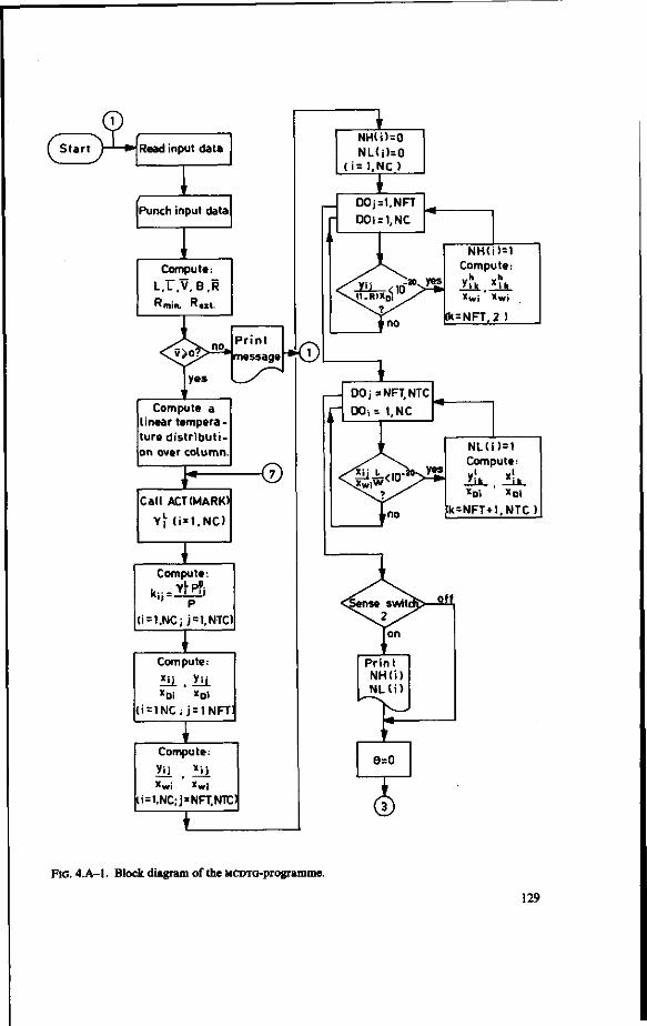
Read input data

Punch input data

Compute; L.r .V. B.R

Rmin. R«it.

Compute a linear tempera­ture distributi­on over column.

Call ACT (MARK)

Y-- (i = 1.NC)

Compute: k . . -YtPTj

" P" (i=1.NC; j = l.NTC)

Compute:

* i i Y i j

(i = lNC; j = 1NFT:

Compute-

*u X w j X

li = t.NC;j = NFT.NTC)

NH(i)=0 NL(j)=0

( i = l , N C )

<D

DOj=1,NFT H DOi = 1,NC

NH(i)=l Compute:

DOj=NFT,NTC

DO,= t,NC

NL(i) = 1

:k-NFT+1,NTC )

FIG. 4.A-1. Block diagram of the MCDTG-programme.

129

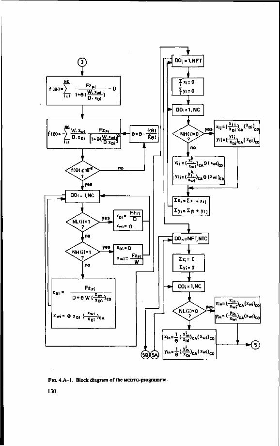
1 NC

i+e(

I D.xDi

f(e>= -W-x« FZ|=

Z_D.xDi [ l + e { ^

DO. r 1 NC

FzFi

D*ew(^r)co >Di

| w i = e « o i ( - ^ - ) c

^ | DOj = 1.NFT

;;

H DOi=1,NC

X i ' = ( ^ C A 6 ( » w i ^

Ix-, = Ixi + X, j

DO„ = NFTNTC

I X J = 0

£y;=o

DOi = 1.NC

X i " = ( ~x^ c * ( X w i ) c o

9 *Dl i-KD

FIG. 4. A- l . Block diagram of the MCDTG-programme.

130

(5B) (5A) 1 I X i = I X i +Xj„

I y i =Zy i + yill

Check = 0

j = '

A=(Ixj)j-1

j = j + 1

j = 1

I ter= 1

a M

Call ACT (MARK)

Yij<i=1,NC)

Compute: Y*- P°.

kn = I lLLLL ' P <i = J.NC )

NC A=rkjjX,-1

i = 1

T(j) = T(j)+10

Punch temp, and comp. distribution

FIG. 4.A-1. Block diagram of the MCDTG-programme.

131

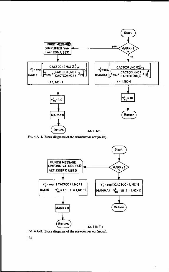
PRINT MESSAGE' SYMPLIFIED Van Laar.EQN.USED

Y;=exp.

(GAM) l ' « CACTCO ti.NC)ZFwC

, CACTCO(i.NC) -, 1 J

NC CACTCO(NC.i) F'J

i =1. NC-1

Y N C = 1 0

MARK= 0

I

Y-=exp.

(GAMMA)

CACTCOUNOXMC;;

[XMC,i

(Return) ACTINF

FIG. 4.A-2. Block diagrams of the SUBROUTINE ACT(MARK).

CACTCO(i.NC) y . 1* CACTCO(NC,

i-1.NC-1

i ) X " J

Y ^ l . 0

f Return J

PUNCH MESSAGE LIMITING VALUES FOR ACT. COEFF. USED

Y^rexp. [ CACTCO (i. NC) 1

(GAM) Y[;c=1.0 (i = 1,NC-D

Y- = exp [ CACTCO ( i , N O ]

CGAMMA) Yj;c=1.0 (i = 1.NC-1)

MARK=0

(Return ) V y ACTINF1

FIG. 4.A-2. Block diagrams of the SUBROUTINE ACT(MARK).

132

PUNCH MESSAGE. Van LaarEQN.USED

Compute: ZEE(i)=ZF(i)

i = 1.NC

'̂ CACTCXKn.i) n -̂CACTCO(i.n)' "'

i= t.NC

Compute:

Yj-=f{ZEE(i).CACTCO<y)}

[GAM) i =1.NC

MARK=0 Compute:

Yi = t ZEE(i),CACTCO(ij)

tGAMMA) i = 1.NC

(= Return J

Return

COMPLETE SUBROUTINE ACT (MARK)

FIG. 4.A-2. Block diagrams of the SUBROUTINE ACT(MARK).

133

> > V X -J u »- o. a. •-• z z i o i o a

U>sl • Z • *« * — m

» U T + ^ » N > » > O «

X I I I I I i z z z z z z

: H o * O O f <

c z u z z -»- < t -z I a

a. u. *o $ « j

o - j a m

^3C H 0. -1 (0

M

-J

a

* z H Z

a a»- a.

9 • -J

( K U U l t m -< t - z a * x

— * - l U J — & r+ l - ^ t • 1 - II Ul

• <->-• *"•»/»-» z — Q. • «4

a j < + - z x t-»o o a -) a. u

i O «

« * z tO — H iH »- _J

u. a o < z a UL u

a -i z o — X X X

8 8!

z

o

< -J -J

t -(A

a

H -

z UJ z 5 9, 1 3 o t -_i

X

Q£ O U.

a g X J -Ui X

</) UJ

a a U l 13

UJ - 1 UJ

X

•-

X

< a o o Of

a. o z i - m Q£t-

< »/> t - •-• to a

,-o X J X

— rf> m rx

m * >-

7-.S5 a A a (/) ~ , H X * < . _ l — X » >- ift

? ; - = O x <n x • > ^ X

— * • D <o— eo O

«-*» — » < * X if» « w e o x ^ - i -0 . - X - X

— x — - a « X i f t > *

— trt co m — 1 - ^ — .MU, < • X • ISl tf> SO X « • o . ~ X - -U O > X i A • X » • -H

— v — *» a. a> * <o co eo

»«f> J X X — -« Z X .0.

G e o — « — t—— to co m Lt Q — — -« < X X o — L J X Z X 1 -

O H * U J x » x a > • n x o » X • i/> _l 3« X ^ > U ) X >- * J • I • t - >- O X S U. to t - • X z * • -x X » •* o X

* <J. z x x O f - » D > -X z n o » > * O * -J * »-» Z X z

O Z U i O • X • Q i f l l X — • • z • H O D •

X • - o x < t - • * O K t f l Z * X « ! / ) *

U. U. » * J Nj • > UJ U_ • a — LU z ^ x a:-si * 0 . _ l UJ * X » x a ac oc

t - * » UJ <

< z u — • X H - Z * -J X * D < • < Z U. i_ t -13 U • _J O • » < UJ •

• - 1 - t - Q Z < U. U) » Q. u» • r x * 0 . Q£ • - U EC

t - O n l D < * • - u a I/J Q u. • *

— a » z x x CO u u. » • < — * • N _J(0 UJ o > - • - > > U I U Z U . I L • M h 3 Z » K

um • x < z z z z z z < * - - I 0 J O U X 1 - U. _ l •- X U. * U J

I / I V I I A I / I I A O Z S Z I / ) • z z z z z z Q < / ) * — -1

I o

•^ eo

<** — F^>-

< UJ H I u i UJ UJ u i x • j o u i a z z z z x x z x ^ x x *

H O * U. t/) *H o o o o a o u x » x

^ ft* rt •* u o

or u.

0 .

> _ j a OQ

> »- x U. Q. • to

ce • * * j

o z * H-o « • z

U. KJ

( O M r t i - t ^* H O o u

^ -< Z h I I - Z l - U . L* Z O O U H « Z - . < < H C K 3 K Ui 111 U l - U . a a o c K Z z z

-*

-) -» X

1—

< V) a. •-«

u u Z — 1

- I o u • o z X -<

— a < -H

M — O

^« — ̂ . ^ — \J X X — — 1 QC z — — « U. | U. * U. U. • rsl • o * r+r*ti*t •# — • a a U * • H + r H , S . + x c o t o u j u r n - J J

• O <J« — is) 3 -H.UJU/ O O r t W h i f l Z - O n H

o t - < — u * a n ( O Q Z Z m - z a H <

< - • o: z - n x d o u j u r g o u a : O N O U . _ J U J _ I

u, — * u .

— * a — 1 e- o

a >n t • —t •

— ,0 — l or m —

< •* V o a» * o

> r- • * \ « 1

u. or ^ J - s . < • • U J Q : as — *H o

< J O I O U I 1 1 1

> n •

t- z X — t -UJ X u.

u. o o c c o-oc: a j z

« < N O 4 l A 3 H 0 t 4 )

X X x x x x x x x a a - ^ z z w a u L> u o u u u < B < — M « en m u , x x

z z z z z z z z z 3 3 3 3 3 D 3 D 3

Q a : z i O Q a ; a u . u ) u i s i u j a i i i > ( D i i C " a : a : a . a. o. a . a a. o. o. a .

u u u u u

134

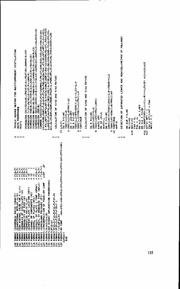
c a v < o * 0 - 1 3 • i/) X J * I •- O X

* O X

co >- m X • a

£ Z D -

* ^ X — - * Z " -> CO *

- o -* ( U ) Z

( f l - O O l H * l X Q£ *J « LO

» < 3 * 13 X • S » X t

• * oca; UJ <

a. i — t • o u • J O • — - - - f UJ •

- Q Z

i c ^ i n j 3 - — H- O «

U(E < UJ < I CO a (JOT X

U - » - « » U U . • • <

! I O U U Z U. U. U k - X Z X M t - 3 Z • X z

X < o _l CO -<

o o o o o o H M M H H H I I I . * U I U»i/>t / )u)*/) i / )ZDZ»/> • Z Z Z Z Z Z O < / > • — _l UJ UJ UJ UJ UJ UJ x » J O U I X X X X X X Z V X X • * * * • • _ n H H O • U . I / > ^ ' O O O Q Q Q U X • *

U » r z— -* U I

« • • - > -> 13

< u o u • - -

• O X X < - I Q >- X C

O O. Z 3 X X O 3 V X *J

t * Z lL C X O H t >• V S

M

O O CD D n

•o — —

^ Q 1 — H H X - • n >- • - —-H

o o u. z IS IH N N *0

^ * < _• — 0 - I X X X O O U . U . X X Q Z Z U . U . Q Q — Z U - Z

CO

%o

< c o

- * • *

WW W WW W 1*̂ WW I •-4H iH d H i-tlTI 1^ tf\ PH IH r"l O U.U.U.U.U.U.— — •— U-U-li-^t

> _l z a a. to

c a. z - • .— z »u— £

u u i i - a . i i

J O J 4 z — - *u

< en-j J << J Z Z — a — O U J 2 £ D t - - < tUX z KUJ X I X N N N

I -UJ O Z U 1 U . O - J O - . — 0. OILH UJ X

o<»- o X < V

o > -I t-xa.u.

j < u . b J Q 3 U I U O i q a i L z X X I X X N N N N N rt W W (O W

- l a ; i*-- , — — 3 o u i» - o */> t- < CO vO z < _l tu UJ O _i a. oca: — a. i t - '

U. U. •- ( U . O O Z V 1 D IO • • 30 . -• H K J S

O m i O O O z u y t j u X X X I I N N N N O > <*\ W m W ^*

UJ Z

xm • x •

mm —i • • u

(MO X

N O If*

U.U. <M

<o mm u. X • • • o o

N N O • u

<<<<<<<<<<<<< <<< <«*<<•*.

135

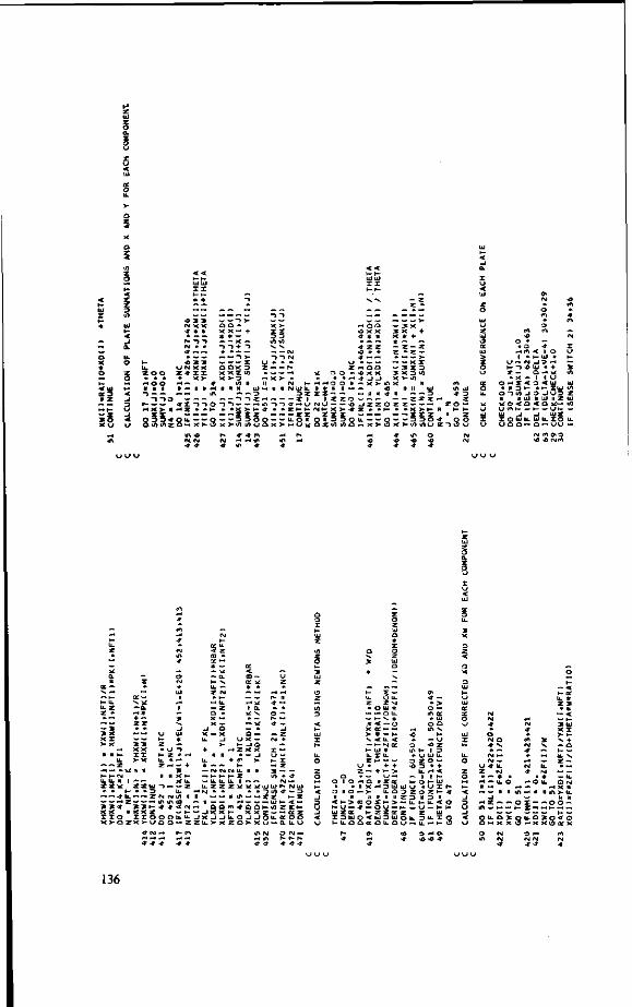
*0 3 3 <M X X •* * * -t O Q — 3 X

0 X X 3 X * * * X * +

; §

t o o

•o 3 3 U N X X z * x i • x >•

s o x : e x i t . e > - 3

3 r-— ~ * z ~> "> o ~> ">•-•» x > n

i to in —

: » » K » » x v t - - * '

I N IN U

» _ _ — — x z -aa — s z 3 0 X X 3 X 3 O t _i _t x >• in » X >• m x n

< o 3 5 * g n — o -\j O 0 m z Q - x > - o J

» Z t~ i - r«l h- x - z z z s . O it o » 5

z o > — «o . >- * ;

I « H - Z Z Z —

I Z Z O Z Z ~ — ~ : » « i - » » x > - 1 - »

O — — 3 3 O •* . X >- O X >- */> tf»u Z '

m <0

• - ~i J>

z — • X —

O ~» I < • II D t -

o ->*/> _i • M U * l o < a UJ J

l o u u .

J 3 H — UJ • + X a ^ ^ i/t i I u

O < Ui UJ * » - X U J «>

3 J U 3 Z

a

* Q£ — ^ *•«

t - u. U. Z Z •

— 3 3 X x i V X

n • t -U .

— z

t - i - rg ix. u. n Z Z X

— z

£K — • v i * — a . • H *

+ — z z

3 3 X X X X V X

•U N II

Z Z U I I - • * 3

u 1 -z

1 -u. z

It

~> . - . - . . * U. ~ - . Z <M

3 3 * X X n o

z — — — l l h

• x x z tf\ •9

u z

H

(M m

*

o (M

+ UJ

1

3

_i U i

• -» 3 X

+

X u.

U. ui (0

< X X O O O u. X > - O Z X > - U O O *-•

z

II

OJ

u.

— a. t - v. u. — z ~

— u. — z o • X — X —

-1 o X — X U, _l

>-+ « B u.

* « — —. <M f *

~ . | _ » _ — u. u. u. z z

-« rs| * • II —> >—

-« Q O — J X X

+

m — a: ^

* * <- ̂ t a . *L * v

— * a ~> u x — t - _J o Z X X • — - I

f l >-

(N U. II II h -U , z

(CI 1 -

z

^ »l * lUJ

• »

o r̂

* X L*

3

«/) • » 3 i f l

m ~ - . z

* o 5 h X X 2

z

to J X J J U O J J O U . Z Z U. V X Z O >- X i j

• * • * • * • * • *

N. <[ U_ < — (— (M (K 1 - UJ * U. X u. Z ^ - —

U * + + Z — + ^ >

Q • — U -H O 1 O -H O • Z CK

• • n x H ^ I U U O H O — >- U . O D II II It II II tl z

< t - > f f l O £ H > « t - u — • * — o<-» — • -LUZCK > - Z Z { £ Z I 3 U J O < U J D U I o * - U . O O H : O I L O U

f- ^ (0 • * »H *

• *

• — »_» o -o z m t- 1 3 • U U J l L

3 Z O — "O 3 • +

U. r-( < — I I I -t - O t - U J U • U X Z O Z 1 -3 1 1 3 1 u. »- u. < — V — t-

Z UJ U. 3 U - X - • U. »- 1 -

3 * * O* i 0 < 0 4

r*-• »

O

s

I

u. o

z o

< - J 3 u - 1

< u

<M O • * V

n* * -(M —

U •* l i-Z (si

• — * • ^ — u. O II >-t • i — n it

- J

^ z O I L O 3 O * * X X

O fM m CM

-*

<«> 3 pg V

•* — ra u. 4- isl

• * — o u.

tft — H It

O X I - z — —

"s. + -» O 1 u. •»* z ~

— u. a NJ

•^ X * if» >- u.

II II o o -

Q U. O 3 0 < O O — x x o ec x

3 ^* (M (M J- • *

cn <N

*

136

j a s t >-1- o » jy * x

— >-H- < I »:

- a z m x *4 X -- • a c

— m — 1 • - — r - O -< CO * X u

CL I - X « * < X » a

— O X — -•o • x m >

* _ l • X - >- O X

• •* O X J Z X I - - D >-! S W • - O * -J

Z X z UJ O • a <yi x

o x UJ •- a u 3

< u.

a. or

a> iiift _i x

w or 111 UJ a a. o z UJ UJ o I -UJ UJ _l _l CM

UJ at-

1- co a

Z Z Z Z LU UJ UJUJ

• * — a , * - - O U U . 3 00 ~ • * - — U J O >-

: X IM»- D

: z z < * ) O O U X

O iflZ 3 z z o </) UJ UJZ • * * § > : Q Q U X

• * LU < J t - H l c u — * - Z * J . o «c • ! l L h l -J ' J O - « UJ *

t- a z ui * a 1 * *

i^-'O or • UJ <

«\X (D N- u or u. *- • z Xor • • < (M _l (D h- > > U. U. • z » a :

1 <

3 UJ CD U - • O 0 : a:

< t -•x. z> m a 9: £ X O UJ U

w u. — 13 N. O — J (NJ *

m < I O 10

Z l * X • X — < . ,-tUJ — O I » • t- « UJ •

U O •- — < -

J Q U X X * U. */) -4

• a. » — o H

0 4 J O * . 3 — • • o u t • r»- o t/» x

I - I I I + X t f l x < o < o r - — D i c

UJ 3 i - « ( - U J O : r - j m i o o x c*» t u i* Difl J O J M i l D - - m - • D — Z m 3 P z 11 ui 1 K i M h i n t i - n<-i i / } ->i- z -• < O < Q • ~* H — • OUJ— H — B O ~ ?

: + — z x z _i _i UJ X N - i o « x i ~ i z — ) — i ( 0 0 3 0 U J U . U J U . t - U . D O — O - I Z D O — o o o r

X - I or _i o o < z ILUUI

u u u ^

0 0 n .-tf-1 I

0 0 0 a H 1 _• ^ r - « - ) - •

X X u> X X x r - •£ u. u w m u u w t M o i z 3 3 0 a a 5

3 3 3 0 0 H a. a a o 0 —

0

T

< O O U J I M I M O U H

U I - U K U W U - U z T 0 : 0 3 D D U . 3

0 CHJ a. Q. a. *- a.

w> 1 -Z U I X UJ

< 1/1

N . "V

(fl -Z N. o>-• - X < 3 x<n X X 3 m 10

X UI <o h- • < X - J 0. X

3 0 (A Z X < m Z X O r-

t- UJ D or 01 3

or < 1- or

z x 0 < — 0 1 - I 3 if* 21 — X or 0

<JI >~ — X a - » —

-* Z X • O IN O

1- * UJ - • X * i/> X X O - t (*> 0 . • X X <f O rg • U H O

O ^ u Z X < - t *

X H- X « z r- # < • ̂ • - 1 - •

— ^) z 0 v i u a z u i H — a. • O Z UJ O X 4 L I O *

UJ UJ t -* I 3 -1

< or x UJ ^

a ** x • UJ UJ 1 - (— X <

<-< Q. X UJX X f*i • 3 0 *

« - H u -o • or 1 •

V

M

n ^ a

V1UJ Z t -O UJ

t- 0. < X a o UJ u t-— ui

Z u. 0

4 I Q O < N O M

h -

UJ_J x UJ or < UJ _l

h- 3 * (*i CO D • 3 LU -

• * U I t-X u D J

fMX < X Z < i f t j l l f f - J J ) I U * a • •* 0. * "v x m-v I m

M l (M fM -

a>

* UJ

n

< ̂ LU X • -X N

< < << < < < < < < x x x z x x x x x x o rororXQTororororaro o 5 0 0 0 0 0 0 o o z U.U.U.U.U.U.U.U. U.U.UJ

O O O O O O O ^ l f M f M

137

o — * o N U • t -

a \ j *><

U U U X l

> o o u • z o o o o w —CD 3 3 Z 3 O

• K m « n g u n i < r- o w l

o Z O Z Z -

it z UJ a. 1 Q W O U O O V ) ( O O v

) O U ) U N U O l f l O Q «

t - m ^ u » - ) - x » : z z -i ) < o u. u, UJ z

Z CC 111

*•« r» pg M e o ^ ^ <*\

O U . U

CLU1U. O I L

Z U U J

lOUJK-— H-VJ

o z <

o — . x • a * -» >

t a x E > -h- o » y> • X

cSfe 2

* « X U. » ** X z 4 — X •

£ * u> X ' J * X - > - o X

~ » < J -

Z co > IJ

iD X rf» >

» • M -to X z z x • 3 >-

X i f l * O - - J

S5Z-

< < D * X i 0 ~ oo X Q. X — X

» * X Ul • u a at of

U )UI

« o

» ** • < z u -

0 < U J U J Z Z 0 — o

D O . 1 z

U1U.O - J O U * Ul ~ ec - x i -« X ~ - l Z K O ; 3 - »- z t - K < \J O Z Q £ < L <

<< Ul Ut J z z w - « « x I - t - <

3 3 0 > O«J

K K K <

S( C U 3 < Z

tf> I/HJ-*

U) * CO X

o> * m _j — Q. iH Z o * • * u — so — H- tf\ — <D U •-• Q — < - X X O H X z

z z z z o o o o

z z z z o S S o

I1:

X < o -

— o. ec

X v t o • —Q. •

- «<->U,

- UiO >-

o u i u z X N H - 3

( J O z z < • -O 0 * - » X t-—«- z u u ) V ) Z 3 1 Z XQ v> -UJUJZ • -

z z z > > - « s • u a o u x

3 « • U. I - h-• J Q

< U I • t - o z ui * a X * • t - W 0T • UJ <

n X d

u. •> •

N - I C O

*- > > U_ U. * z * or • X <

Ul ( -X - u I - > 3

— h Ul t -*-\J < < < a u -

< u or

DC I ^ < H •

© —

* •

I O M O N

• z z a t-I • Ul z i 3 • •

- z o o o

• ao u -* «M N N +

z o o

tl z — Ul f -

w < — a: U.U. u» Ul UJ

\J o

H-UJ

Ul u

UL 3 §

O O O \J —

- • K z u z o o o b M O M O u o o M i a

3 O O O i n m -* CM <-* o * ^ •* * m

O W l .

N I L

o o r- o « N • H-fM

I U I O 3

- Z « k. c « or

§si§§s;

UJ Ul — 00 3 3 Z O z z — . I « « x • - « . _ » -

^ • »- H> — h - ) £ 3 Q, Z - Z Z X Z K k Z -

n . c o o o < o < u i o *n H Q U U U U X K U 3

\J\J U U U

138

3t * ifl - 1 2

>- • J » X » t - > O X

D

• X -1

: • • x z • 4 0 X UJ > z t i -- • D>- U : x 10 * — » O • _ ! U. t z x z u.

< t - * •

: UJ z • o UJ

mco ~ • — m —

— * ^ * * t -* \ x »co < H i 00 —tO

• x - t n CO * X < • — — X o — V«f» X • <0

— 13 I <

a x

*> Q —UIZ « X « rs| » a. J U * * • x o K a:

»- • • UJ <

. U ^t—• H l t K < Z U. 1 - 1 -

< I -I - J O I D <

i -I O 3

x > o n u • » X — •>

— — > . * - . —* 40 CO * GO CO * —~ —— • 0£3t_J m « «o < x z -*0. — X * • - » o -U——OHUl < O I X «• < L

X Z X h- O f.

c o z z z z z : i OTUJIiJ UJ UJ UJ L - o izz i n :

< • J Q UJ • Q Z C

a. or i - <->oe

k •> <M _ J < D 4- <n .-< u

J X U. U. • — • _< Z b -- 3 Z »Q£ .-t

. M « 0 » I L I - t n * - < i f l Q Q O O Q O U X

O I r-t X 1 * — - ) Q 1 - « . H l u l l « - « - > • J O u n O v j • * «J J « « 1 — Z - " N — z « - — Z -or i- — u * z — — z J < X < « O - I Z o: • o < < «£ U X W X -< * 3 <M X X 3 • * r o c H Z Z K I - H x x i - o • * i t D o u o < < < w u o < < w r / - . a - u - z a o o x t t z o o o o c i u

o •-« o o o o o •-• o *M

z uj < — > -x. < a z uj — _ to u. — O

J? - * «

O 0. — I- >- u < «/> < J » Ul - - I/) • ->- r- z w> z ~ ~ UJ I Q - • Z

U O i_ « z Z U. lit u. u. Z ' J O o o a. u a:

x «> o l/l Otf\

X Z >- I - O • • « / > • X

Q M > U J X • X tL >-* -> X o »

1 • U 1 J S x ^ * < o x >- • J * X • I- V O X * U. I/} t- » X Z • • X

— X • • * O X

— * t_» 3 < a z u X X • c X x ~ . < * Q. C

4 — » _ f s | • > * eo < • Q -> — ifl i i x a • z a . a J I I E < - • X C

O UJ U. I- Q

< UJ a _i »-

O 3 <

I U U I - J « UJ < I-X u

I/)

• — * < Z l. • « » £ » • ; •» — — x * ; - * 'U. t - < Z b " J < O U -3 » ( / ) • > « - — Q . i - , _ ». s m u < u- u C ^ • i^ • 3

- » — a oc ^ J < o : m o

^3 — • -I- X

UJ 3 — -I O X UJ a:

X 3 I

B — m i - » * r t j O r t U O >" •• < Q X X — < U X li

x z x t - u h - ^ a UJ U l f l • z z z z z z < • • -- ^ O O O O O U X I -f_ M « « M « I i

Z O Z Z Z Z Z O t O ' M O C t u t i l b J b J u J X * -

i - m x x x x x x v > U 3 * - — — « — O » l < V ) O O O O Q U X

* ^ - * u.

- _ I < X < •

t » - Z Q : H 'i <̂ u. o O o

O II '

E X Q : t < < J O X

* a, H H - t — x U - < M U I ^ z o * » U • M —

I _ , I -> KJ — - > *

<J • < -» * U > Z - • VJ * — z

z « z

i K i o • « < < i r " - <M X X X 3

- ^ o '

u u u u 139

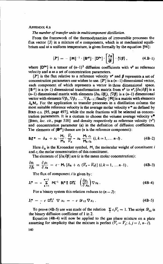
APPENDIX 4.B

The number of transfer units in multicomponent distillation. From the framework of the thermodynamics of irreversible processes the

flux vector {J} in a mixture of n components, which is at mechanical equili­brium and at a uniform temperature, is given formally by the equation [94]:

{J«} = _ [M] -1 • [B"»] • [D»«] • T 0 l • M*} , (4-B-l)

where [D1™] is a tensor of (n-1)2 diffusion coefficients with v* as reference velocity and a as a set of concentration parameters.

{J"} is the flux relative to a reference velocity v" and fi represents a set of concentration parameters one wishes to use. {J°} is a (n-1) dimensional vector, each component of which represents a vector in three dimensional space. [B"*] is a (n-1) dimensional transformation matrix from v* to V,[da/dfi] is a (n-1) dimensional matrix with elements (dot; /3/J,), {Vj8} is a (n-1) dimensional vector with elements V/?i, V/J2 ... .V/J.,-1; finally [ M] is a matrix with elements SikMt. For the application to transfer processes in a distillation column the most suitable reference velocity is the average molar velocity vm as defined by BIRD c.s. [95, page 497], while the mole fractions will be selected as concen­tration parameters. It is a custum to choose the volume average velocity v" [BIRD, loc. cit., page 518] and density respectively as reference velocity (vfc) and concentration parameter (a) in the definition of diffusion coefficients. The elements of [Bab] thence are (n is the reference component):

BJF" = dik + xi • -£' • - £ - xk -JJ-^ (1, k= 1,... »-0 . (4B-2)

Here d^ is the Kronecker symbol, M, the molecular weight of constituent i and Cj the molar concentration of this constituent.

The elements of [da/dp] are (c is the mean molar concentration):

| | = | ^ - = c • Mi {8ik + a (V„- Vk)} (i,k=l,... n-1). (4B-3)

The flux of component 1 is given by:

ir = - V Mr1 Brs oti f|^-)v*». (4B-4) t = l \OXk/

For a binary system this relation reduces to (n = 2):

Jf = - c D11" V x . = - c 3>i2Vxi . (4B-5) To prove (4B-5) use was made of the relation 'LciVi= 1. The script 3>l2 is

the binary diffusion coefficient of 1 in 2. Equation (4B-4) will now be applied to the gas phase mixture on a plate

assuming for simplicity that the mixture is perfect (K, = V}; i,j= 1, n-1).

140

The matrix [Bm" ] now reduces the diagonal unit matrix [ U], while [dp/dx] also becomes diagonal:

[ B - ] = [ U ] , (4B-6)

• c[M]. m Equation (4B-4) can now be written as (yk indicating the gas phase mole

fraction): ir = - c 2 D'k Vyu. (4B-7)

i t = 1

The definition of the overall gas phase mass transfer coefficient following the convention of BIRD C.S. [loc. cit., page 639] reads for a binary system of species 1 and 2:

J In i_ = n ko*loc Ajl = — Jill , , . _ _. I phase phase (4B-8) boundary boundary

n is a unit vector normal to the phase boundary pointing inward to the liquid phase and Aj^ is the concentration difference between bulk gas phase (time smoothed and surface averaged) and the equilibrium composition of the gas phase ( < j \ > *)• Neglecting the dependence of the mass transfer coefficient on the mass transfer rate and averaging over the time smoothed total interfacial area in the liquid layer on one plate the dot (•) on kog- ,oc. and the subscript 'loc' will be omitted in the notation. From a mass balance on a differential dimen-sionless height of liquid (d/) the equation (4B-9) follows:

VJi" • Ji" = <JiM> = koo(<yt> -<Pi>) d / = -£ dyi. (4B-9) As

Comparison of (4B-9) and (4B-5) and (4B-4) suggests the following definition of multicomponent overall gas phase transfer coefficients [cf. DIENER and GERSTER]. {<J">} = [ M ] - 1 [ B " - ] [ K J G ] - g l { A y } d / = ^ { d y } . (4B-10)

This equation yields the following set of differential equations:

^ { A y } = - [NOG] {Ay}, ( 4 B _ U )

where the matrix [NOG] is defined by:

[NOG] = 4?" [Ml""1 " [B"" 1' \*-<>G] • ffl • (4B-12) V

Integration of this set is possible with the PEANO-BAKER method, considering the elements of [NOG]to be constants. The boundary conditions are {Ay} = = {Ay}e for / = 0, and {Ay} = {Ay}0 for / = /.

141

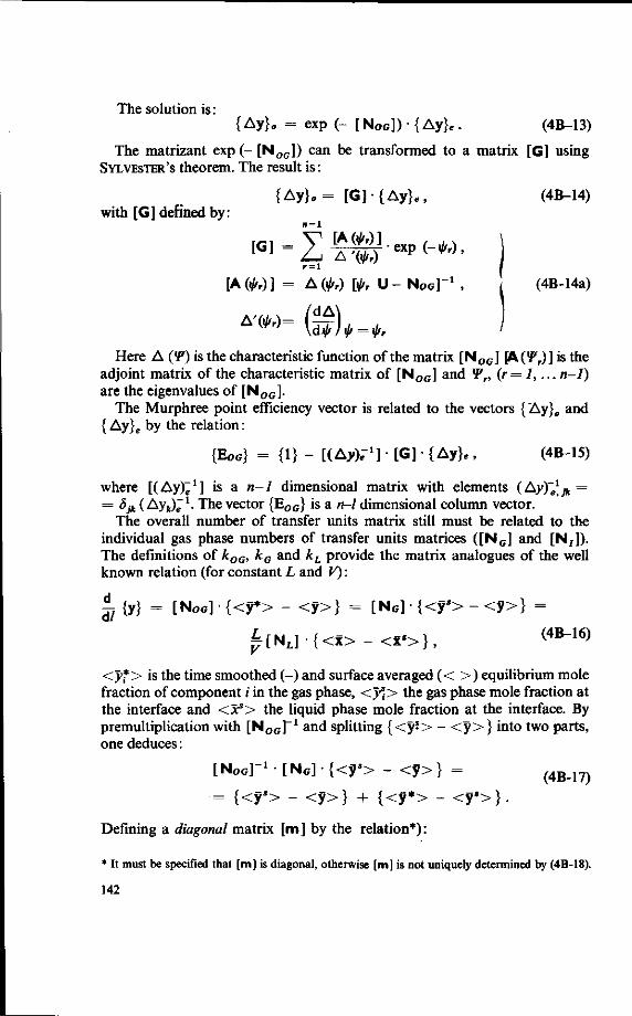
The solution is: {Ay}„ = exp (- [NOG]) • {Ay}e . (4B-13)

The matrizant exp (- [Noc]) can be transformed to a matrix [G] using SYLVESTER'S theorem. The result is:

{Ay}0 = [G ]{Ay} e , (4B-14) with [G] defined by:

[ G ] = 2 A '(*,) CXp ( *'>' r = l

[A(*,)l = AfcM [i/,r U - NOG] - 1 , j (4B-14a)

Here A (f) is the characteristic function of the matrix [NOG] [ACFr)] is the adjoint matrix of the characteristic matrix of [NOG] and Yr, (r = l,... n-1) are the eigenvalues of [NOG].

The Murphree point efficiency vector is related to the vectors {Ay}0 and {Ay}e by the relation:

{EOG} = {1} - [(A?),-1] • [G] • {Ay}e , (4B-15)

where [(Ay)"1] is a n-1 dimensional matrix with elements (Ay)'*jk = = djk(Ay^i~l. The vector {EOG} is a n-l dimensional column vector.

The overall number of transfer units matrix still must be related to the individual gas phase numbers of transfer units matrices ([NG] and [N7]). The definitions of kOG, kG and kL provide the matrix analogues of the well known relation (for constant L and V):

j t {y} = [NOG] • {<?*> - < y>} = [No] • { < r > - < y>} =

^ [ N J { < x > - <!«>}, (4B-16)

<y*> is the time smoothed (-) and surface averaged (< >) equilibrium mole fraction of component / in the gas phase, <ys

i> the gas phase mole fraction at the interface and <xs> the liquid phase mole fraction at the interface. By premultiplication with [Nog]-1 and splitting {<y J> - < y>} into two parts, one deduces:

[ NOG]"1 • [ NG] • {<y s> - < y> } = ( 4 B . 1 ? )

= {<ys> - <y>} + {<y*> - <ys>}-

Defining a diagonal matrix [m] by the relation*):

* It must be specified that [m] is diagonal, otherwise [m] is not uniquely determined by (4B-18).

142

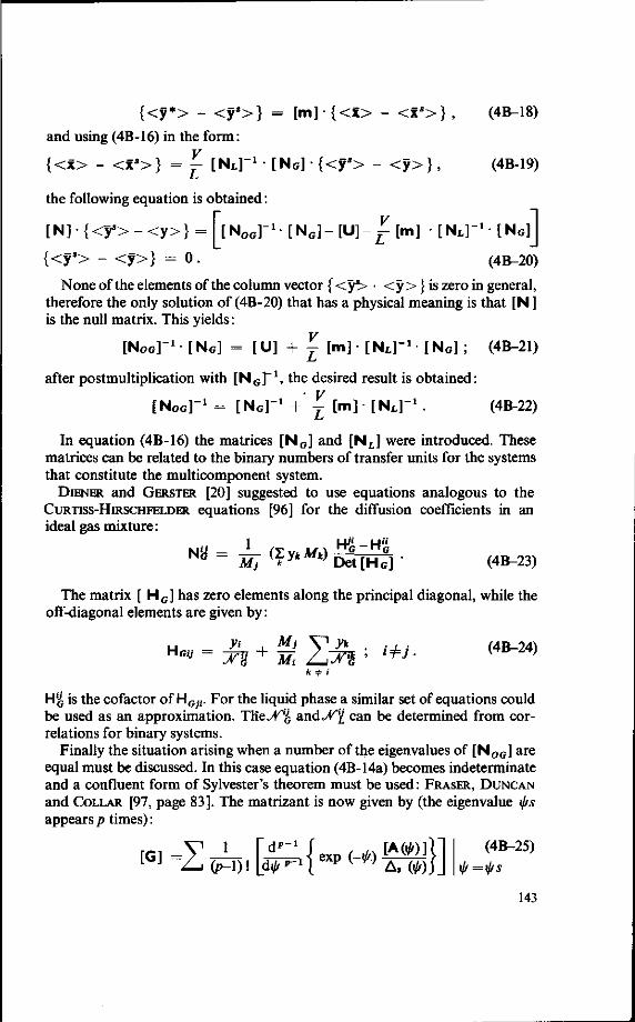
{<y*> - < y s >} = [ m ] { < x > - < x s > } , (4B-18)

and using (4B-16) in the form:

{<x> - < x s >} =j- [ULrl{^o]{<r> ~ < y > } , (4B-19)

the following equation is obtained:

[N] {<y s >-<y>} = [ [NO G ] -1 [NG ] - [U]-^[m] -[NLp-INclJ

( < y J > - < y > } = 0 . (4B-20)

None of the elements of the column vector { <y> • < y>} is zero in general, therefore the only solution of (4B-20) that has a physical meaning is that [N ] is the null matrix. This yields:

[Nool^-INc] = [U] + j - [ m J - I N J - ' - I N o ] ; (4B-21)

after postmultiplication with [NG]"', the desired result is obtained:

[NOG]- 1 = [Nc]"1 + -£ [m] • [ N L ] " 1 . (4B-22)

In equation (4B-16) the matrices [NG] and [N t] were introduced. These matrices can be related to the binary numbers of transfer units for the systems that constitute the multicomponent system.

DIENER and GERSTER [20] suggested to use equations analogous to the CURTISS-HIRSCHFELDER equations [96] for the diffusion coefficients in an ideal gas mixture:

N « = i ( ? ^ M ^ s l [ R f t - (4B-23)

The matrix [ HG] has zero elements along the principal diagonal, while the off-diagonal elements are given by:

" - - & + M 2 ^ ' '«• <4B-24)

k + i

H'G is the cofactor of HGji. For the liquid phase a similar set of equations could be used as an approximation. THcv^g and^T^ can be determined from cor­relations for binary systems.

Finally the situation arising when a number of the eigenvalues of [NOG] are equal must be discussed. In this case equation (4B-14a) becomes indeterminate and a confluent form of Sylvester's theorem must be used: FRASER, DUNCAN and COLLAR [97, page 83]. The matrizant is now given by (the eigenvalue \j/s appears p times):

y _ L U'-1 JexP(^) [A(»)]jl I (4B-25)

143

where A s ( ^ ) = 7 7 (iff- ty „), the summation is taken over all distinct values i// s; As( if/) = 1 when a// eigenvalues are equal.

As an example this most degenerate situation will be evaluated, which arises when the matrix [NOG] is given by:

[N 0 G ] = [U] MG. (4B-26) Now [A (i/0] becomes:

[A(tfO] = {iji - JTOGT'2 [ U ] . (4B-27)

The matrizant thus is given by:

[G] = L (-*) [ U] - exp*1' (-*) (*- r̂OG) [ U] +

+ CTP<32)!("^)(^-^>o)2[U] + .... + (g^exp<»-2»(-^)(^-^bGr2

']*-t U] |.,f = ^ = exp (- ^ 0 G ) [ U ] . (4B-28)

This result could not be obtained from the Sylvester theorem as stated in (4B-14a) one should note.

APPENDIX 4.C.

Computer programme for multicomponent distillation with plate efficiencies included (MCDTG-EFF).

This appendix contains a description of the MCDTG-EFF programme without giving a block diagram. The logic of the programme is very close to the MCDTG

programme, therefore a FORTRAN listing with a more detailed description than that given for MCDTG is felt to be sufficient. The nomenclature contains only new variables introduced in MCDTG-EFF as compared with MCDTG. The pro­gramme is made suitable for an ELX-8 digital computer with a FORTRAN com­piler. The CALL LINK mechanism is replaced by a SUBROUTINE structure. A typical distillation calculation of 5 components and 10 plates requires 0.8 minutes computing time.

Nomenclature:

WW Height of weir [in.] FF F-factor (eqn. 4.59-60) in

[ft./sec (superficial) yj lb./cu. ft. ] H L Liquid flow rate per foot of weir

length [gal./min. (average liquid flow width), ft.] DL Mean value for liquid phase diffusivity [sq. ft./hr. ] Z L Length of liquid travel over tray [ft. ]

144

SCG Average Schmidt number of gas phase (Scg) FNG Number of gas phase transfer units (JVG), equal for all com­

ponents FNL Number of liquid phase transfer units (^ , ) , equal for all

components ZC Auxiliary variable in correlation for JfL, (eqn. 4.60) ACTC Subroutine calculating the activity coefficients MARKT Flag indicating wether temperature dependence is included

in activity coefficient equation EOG Murphree efficiency TC Bubble temperature of distillate PKO A-factor for distillate DK Difference in K-values of a component on two successive

trays (A Ki}) DX Liquid mole fraction difference for a component between two

successive trays (Ax^) FM Slope of equilibrium curve (/n,) FNOG Overall number of transfer units based on gas phase.

The programme starts with reading a title card followed by a card containing input data on the bubble plate design specifications (weir height, liquid flow rate per width of flow, length of liquid travel over the tray, /-"-factor), liquid phase diffusivity and Schmidt number of gas phase. A set of efficiencies of the reboiler is read next to these data. The rest of the input is exactly equal as described in APPENDIX 3.B for the MCDTG-programme, VBAR is checked as usual and now JVL and JVG are calculated using the correlations discussed in the text (Engineering units are used). When VBAR remains positive a linear temperature distribution is calculated from the estimates BPMV, and BPLV. ^-factors are calculated and the first iteration is started. Up to the third iteration cycle the programme calculates as if the trays were ideal. Then, at the third iteration cycle, £OG-values are included in the calculations. From statement 1001 up to 1250(DIST1A) the AT-factors for the distillate are calculated. For this purpose in the first two iteration cycles bubble tempera­tures for the distillate composition were already performed. From the distillate composition, its set of ^-values, and the composition of the liquid on the first plate with the appropriate set of ^-values, components of [m] are estimated, using equation (4.72).

Then equations (4.32-4.39) are used to calculate the YXD, XXD, YXW and XXW ratio's over the column. The £OG-values are continuously calculated from AT-values and liquid phase mole fractions. The Fog-values of water(NC'th component) are based in the assumption that for this component the liquid phase transfer resistance is zero. Each £OG-value is checked as to maintain positive flow rates.

Next the separated light and heavy components are detected, using equations (4.40-4.41) when such components are detected.

145

The programme continues with calculating 3; once a solution is obtained corrected mole fractions are calculated and mole fractions on each plate (S) are summed and checked to be unity, when the criterion | Z -1 | < 70"4 is not satisfied a new temperature distribution is estimated from bubble temperature calculations using equation (4.44) and (4.45).

The activity coefficient calculations again use VAN LAAR multicomponent equations. Provisions were built in to use equations with temperature depen­dence included (by giving the flag MARKT a value different from zero).

When bubble temperature calculations are completed the programme starts a next iteration cycle with calculating new A-factors for the distillate.

c: miELK sBXJes MEmD rot MnCTCtMUiuurr rasmuoicm, s n s ra c iES ; c: Bcuaao cnoauwc; C: nisrsA; C: MCDBB - BT; C: ;

I CACICO(8>8),CFS0(8,6)<F80(8)<aUMt(8,l;); i SD(8>i;),xxD(8<i;)>xxn(e,i;),BW(8,i;);

DDBEiai IH(8),lL(8),YHIl((e,15),ralW(8,15),IIJCD(8,15); IXD(8),IlK8),X(8,15),T(8,15),sao(l5),Smr(l5),ILID(8,15); I T(l6),I*<8,15),2*(8),au«8);

mDHHXCn ZEE(8) ,EOO(8,15),F*D(8); CdtOI C*3TCO,CJSAT,PSAT,<U»««,T,rc,CT,{^XIL,riD,XM,IM,m,M,X,Y,SWI,SWr,F,^^ K,»rc,»rT,x,J,i,»ci,Fxi,Hm,»T2,WT3,THBTA,FiMrr,i)Httv,ittrio,iHog*,s^ ISm,ITBI,Zffl,SS,Iffi,3tK3»CI,IO,3IflPB,BIJin,EL)QiW,VBm,RB«H,Pli,nr,I,)l«a,WI,l,«,m,II,YHM,XH^ a n a nDjnumG , M R B ,Tc,ntD,saEOF; READ 151 j FCRMMF (80BOOOOOOOOOOOOOOOOOOOOOOOOOOOOOOOOOOQOOOOOOOOOOOOOOOOOOOOOOOOOOOOOOOOOOOOOOOOOOO<x}j

PRUT lsi j REM) 102,W,JT,HL,EL,Zl,3CO; READ 101,F,D,«,B,fT; READ 101,Cm,BC,EBK,B?LV,PI; •&CI;

KEU) l60,(EDS(I,IIC),I-t,K)i ID 1 K-1.K;

146

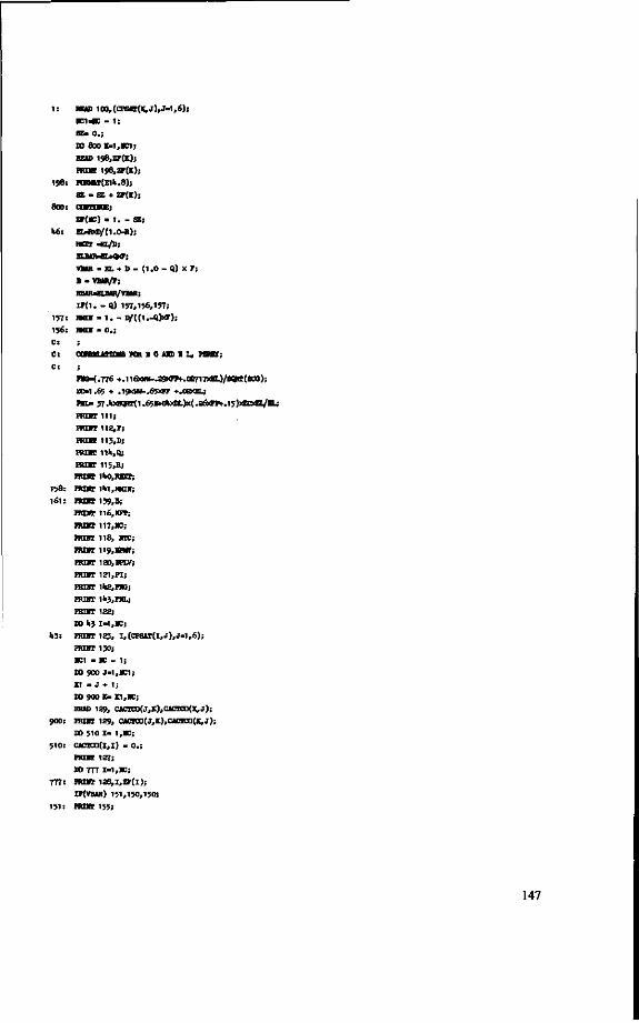
t : B I D 100,(CPSAT(K,J),J-1,6);

K 1 4 E - 1;

SZ- 0 . ;

ID 8 0 0 X > 1 , K 1 ;

READ 198,ZT(K);

m m i98 ,2y (K) ;

198: mMa(E i>> .8 ) i ffi - ffl + ZT(K);

ZF(K) • t . - S ;

M : EL*XD/(1.0-B);

REH ^L/D;

EUAR-ELXOT

VIAK - EL • D - (1 . 0 - Q) X F;

B - VBAR/F;

RBAR-ELBW/ra«R;

I » ( l . - 9 ) 157.156,157;

157: s u n - 1 . - D / ( ( I . - Q ) » ) ;

156: R O T • 0 . ;

C: ;

Ct CCHIELATXDJB KR M a AID M X» PERRT;

C: ;

raa-(.776 +.n6xWW-.29XIT+.0?71TxHL)/Sl»tr(SCO);

ZC-1 .65 + .19XW-.65XFF •.02XHL;

B B > 37.lu«BT(1.65E«*xia.)x(.26xrF+.15))«CXZL/HL;

F 8 m 111;

ram 112.F;

ram 113,1);

ram n u . d ;

ram i i ; , R ;

H t m lb0,REXT;

158: ram 1 k 1 , m i l ;

161 : ram I39,B;

ram 1l6,HFT;

ram i i 7 , K ;

ram 118, KEC;

ram ii9,aw; ram 120,BH.V;

ram 121, P I ;

ram i t e , m ;

railfr lb3,Fl)L;

ram 122;

DO !>3 1 - 1 , K ;

* 3 : ram 123, I , (CTSAT(I ,J ) ,J -1 ,6 ) ;

ram 130;

K 1 - HC - 1 ;

10 900 J-1,DC1;

XI m J + 1;

CO 900 K- K1 ,K;

SEAS 129, CACICO(jr,X),CACTDD(lC,J)i

900: ram 129, CACTC0(J,K),CACIC0(K,J);

DO 510 I - 1 , K ;

510: CABTCO(I,I) - 0 . ;

ram 127;

DD 777 1 *1 ,K;

777: ram I 2 8 , I , Z F ( I ) ;

U(VBAR) 151,150,150;

151: ram 155;

147

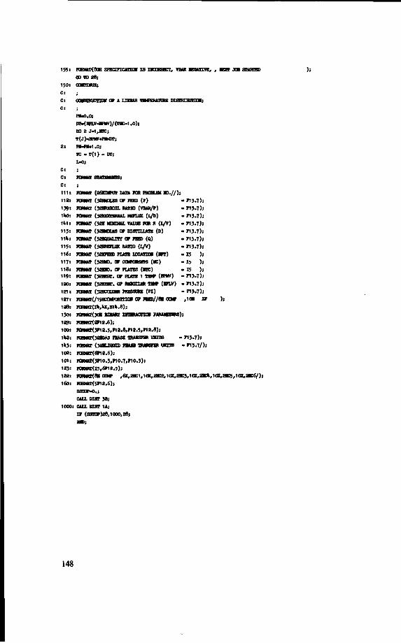
150:

C:

C:

FORMAT(8OH sracincAnai i s

00 TO 28;

CUBl'lEUE;

HC0RRECT, VBAR XBQATIVE, # REX? JOB STARTED

OUBtUKUCTIOE OF A LIVEAR TEMPERATURE SISTRXBUnOE;

C!

Ct

C:

t i l t

112:

139:

1U0:

l M :

113:

l U i

115:

116:

117:

118:

119:

120:

121:

127:

128:

130:

129:

100:

1*2:

1*3i 102:

101:

123:

122:

160:

HMl.Ot

OT-(BPLV-BfW)/(T»C-1 .0);

SO 2 Jal,RC; T(J)«EPMV*PK>OT;

PMH-1.0; IC - T(1) - DI; L-0;

FORMAT SXATEMCRS;

FORMAT (a6Hiiow DATA nit PROBLEM H O . / / ) ;

FORMAT (32BHLES OF FEED (F) - F13.7); FORMAT (32HREB0IL RATIO (VBAR/F) - FI3.7);

FORMAT (32EBOHOAL REPLUX (L/D) - F I 3 . 7 ) ;

FORMAT (52H H D O U VALUE FOR R (L/V) - F13 .7 ) ;

FORMAT (32DOLES OF DISTILLATE (D) - F13 .7 ) ;

FORMAT (32BJJAUTY OF FEED (4 ) - F I 3 . 7 ) ;

FORMAT (32HREFLUX RATIO (L/V) . F13 .7 ) ;

FORMAT (32BFEED PLATE LOCATIOJI (OT) - 15 )

FORMAT (32HK). OF COMfOTERTS (EC) - 15 )

FORMAT (32HH0. OF PLATES (RC) - 15 )

FORMAT (32HEST. OF PLATE 1 TEMP (BPMV) - F13 .7)

FORMAT (32HEST. OF REBKLER TEMP (BPLV) - F13.7);

FORMAT (32BCDUMI PRESSURE (PI) - F13.7)

F0RMAT(/l9HCOK?O3m0« OF FEED//8H COM? ,10H ZF ) ;

F0BMAT(Ik,tX,E1k.8);

F0RMAT(30H BUUSt UTERACTIOR PARAMETERS);

FORMAT(2F12.6);

F0RH«T(3F12.5»F12.8,F12.5,F12.8);

P0RMAT(32BMS PRASE TRAISFER UHTS - F I 3 . 7 ) ;

FORMAT (3ZHLigUH) PHASE TRAISFER UHTS - F 1 3 . 7 / ) ;

F0RMAT(6F12.6);

FORMAT(3F10.3,F10.T>F10.3);

FORMW(I5>6F12.5);

FORMAT(8B COMP ,6X,2BCl,iaX,2BC2,iaX,2BC3»iaX,2HCk,iaX,2B£5>10X,2BE6/);

FORMAT(5F12.6);

CALL DI3T 3B;

: CALL DIST 1A;

IF (S3IOP)28,1OO0,28;

148

C: 'inning QKUJEtt K U D FOR MULXX COMUUU' mwFTTTOTTm , EFFI&HKIES;

C: CAX£ULAHm OF K-VALUES FOR FIRST ITERATa* CYCLE;

C: MST3B;

C: ICDIO - EFT;

C: ;

s u m u w i m m a r » ;

DIHEHSIOK CACTC0(8,8),CPSAT(8,6),PSAT(8),<1AI»IA(8,15);

naasna xn>(8, I 5 ) , Y X D ( 8 , 1 5 ) ,xxw(8,15 ) , Y X V ( 8 , 15 ) ;

DIMEHSIOH KH(8),»L(8),YHXV(8,15),XHXV(8,15),ILXD(8,15);

EIwaiSI (Bia) (8 ) ,XV(8) / X(8 ,15) ,T(8 ,15) ,a jK(15) ,SU«f ( l5 ) ,XIXD(e ,15) j

DIMEMSIOd T(l6) ,PK(8,15) ,ZT(8) ,0»M(8);

DDfflBSICB Z£E(8) ,EOO(8,t5),IW>(8);

C O M B CACico,cps«T,PSAT,OAm,T,PX,ZF,OAM,xxD,YXi>,xxw,Yxw,XD,xw,x,Y,suMK,s^

• c , » r c , » T , r , j , i , i c i , r e L 1 i r n , m T 2 , H ! T 3 , r H E n * , n n i c T , i H i i v , R j m i i , D a o i , » ^

lJEm,:rira,Zffi,SS,Iffi,^SUK>,TO,SI^E,T»,K1,EL,ELBAR,VBAR,RBAR,P1l,OT,L,M^

C O M O I rao,raL,Eoo , WHET ,Tc,FK0,sanx>;

C: CALCULATIOH OF K KB EACH CCMFCRKT;

MUX - 1;

CALL ACTC;

10 U J.1,«TC;

n j J I " l ,«C;

PSAT(l)^OT(Cr£M(l,l)4CPSAT(I,2)/(CPSAT(I,3)«(J))<<S>SAT(I,^^

31 HC(I,j)-OAM(l)XPSAT(I)/PI;

U: amnEi «FL- 1;

ram 888;

888: FORMAT (6BDIST1A);

END;

C : THLELE QECDE8 ME29DD FOR MULTXCOMPOHEHT IXI9FILLATX0H, EFFICIETC1ES;

C : MUM PROGRAMS ,CALCULATIBO KILE FKACTia i RATIO S THROUCTXIT;

C : COLIMI;

C: Diaru; C : K D T G - EFF;

C : ;

SUEROUTIHB DiaT 1A;

I CACTCO(8,8),CPSAT(8,6),PSAT(8),GA>«(A(e,15);

I XXD(8,15),YXD(8,15),XXW(8,15),YX»(8,15);

I RH(8),»L(8),YHXVI(8,t5),XHXW(8,15),YLXJ><e,15);

IXD(8),XW(8),X(8,15),Y(8,15),SUKX(15),SU*(15),XLXD(8,15);

DDEBSIOK T(l6) ,FK(8,15),ZF(8),aAM(8);

DIMEKSKH ZEE(8) ,E0O(8,i;) ,FKO(8);

COJMIN CU«aa],raSAT,PSAT,OAI»IA,T,FK,ZF,aAK,XXD,YXD,XXW,YXV,XD,W^^^

BC,ltTC,lOT,lC,J,I,llC1,FXl*»m,llFT2,IFT3,TBElA,FlllCT,I]HOT,R^

DEU»,ITHI,ZEE,S3,DB,StK31JM3,ro,SL0PE,TJI,in,EL,EIJAR,VBAR,RaiR,P>,OT,L,MAHC)KRL,H,^

C O M * na,ra.,ma , M U S T ,TC ,FKD,SSTOF;

C: ;

C: CALCULATIOH OF X/XD ADD Y/XD RATIOS;

C: ;

Muaoo; 13! Lr f / t l ;

I P ( L - I ) 1000,1000,1001;

1001! 1011(10 K-1,NC;

ss - 0.; C0H20 1-1,IK;

IF(CACT00(K,I)) ll»50,lWlO,lli30;

11)30: SS-SS +Y( l , 1 ) >CACTC0(I,K)/CACTC0(K,I);

149

00 TO 1U20;

lUlO: SS- SS • Y ( I , 1 ) ;

1U20: COKTHIUE;

ZEB(K)-Y(K,1)/SS;

l i n o : cawrcnuE;

D01250 M-i , lC;

SS > 0 . ;

SB - 0 . ;

DD1260 I - l .BE;

SS - SS + CACTCO(M,l)XZEE(l);

ir(CACTCO(l,M)) 1225,1215,1225;

1215: 101270 K-1,1K;

1270: DB - DB + CJCTCO(I,X) X ZEE(l)xZEE(K);

00 ID 1260;

122S: 10 1280 K -1 ,K;

I?(K-M) 1228,1280,1228;

1228: DB - DB + CACTC0(M,I)/CACTC0(I,M)>CACTC0 (I,X)xZEE(l)xZEE(X);

1280: CtwnmjE;

1260: ctwnmjE;

OAN(H) . EXP(SS - DB);

1250: OOmaUE;

DO 1003 I-1.1K;

PSAT(I) - BCP(CPS«T(l,l)<CT>SAT(I,2)/(CPS*r(I,})-f!K;)<«PSAT(I<'>)XTC + CPSAT(I,5)XTCXX2 + CPSAT(I,6)xU£Q(TC) ) ;

1003: PKD(l) . 0«M(I) X PS*T(I)/PI;

DO 1222 I - 1,HC;

DK. PKD( l ) - fK( l , l ) ;

DX- Y ( I , l ) - X ( I , 1 ) ;

FH - FK(I,1)+ X (X,1)XDK/I1X;

IF(FM) 11*00,11*01,1U01;

11*00: FM » 0 .00;

11*01: FSOC- 1 ,/ftC * FK/(F10>K);

FHOO • 1./F80G;

E00(I,1) - 1. - EXP(-nDO);

1222: CaKTIHUE;

E0Q(]K,1) - 1. - EXP(-FJG);

1000: DO ; 1-1,HC;

YXD(I,1)-1,0;

5: XXD(I,l)-1.0/FK(I,l);

DO 7 J^.IFT;

DO 6 I-1,«C;

IF(L-2) 300,300,301;

301: DK-FK(I,J-1) - FK(I,J);

DX - X(I,J-1)- X(I,J);

I F ( j - 2 ) 3500,3500,3603;

3603: IF(DX) 3500,3501,3500;

3501: EDO(l , j ) -EOG(l ,J-t) ;

GO TO 312;

3500: COVTmUE;

FM- PK(I,J) + X(I,J)XDK/DX;

IF (FH) ll*02,lU0},ll*03;

11*02: FM - 0.00;

1>*03: FBOB- 1./FB0 * FM/(nUX>);

FBOO- 1./FKX);

HXt(l,J). 1. - BXP(-nOO);

BOO(«C,J) • 1. - EXP(-FHG);

312: D O - EOO(I,J-1) + (1 .-E00(I,J-1))>«/HI(I,J-l );

IF(Dal) 1306,1306,1330;

150

1306: B0O(I,J-1) . ( -Bxo.99995/(HC(I ,J- l ) - H) ) ;

00 TO 312;

HCD(I,J) - ( ( 1 . -B )XE00( I , J - l ) +R«niD( l ,J -1) /HC(l ,J -1) ) / IJE»;

IF(YXD(I ,J ) / ( l . -B) - 1 . ) 306,306,330;

306: BER - *XD(I ,J - l ) + (B-l . ) x ( l . -HJJ ( I , J - 1 ) ) ;

IF(IBI) 3oB,330,330;

306: BXKl .J -1 ) - ( 1 . + 5 .K-08)x(1 . - *XD(I,J-1 ) / ( 1 .-H) ) ;

00 TO 312;

3301 X X D ( I , J - l M X » ( I , J ) / * • 1 . - 1 . / F ;

00 TO 6;

300: raE(i,j)«B<(x]a>(i,j-i)-i.o)+i.oj

XXD(I ,J ) -B0) ( I , J ) /PK^,J ) ;

6 : C0HTHUE;

7 : COVTISUE;

C: ;

c: CALCULATION OF X/XV AND Y/XV RATIOS;

C: ;

10 8 1-1 ,MC;

x x v ( i , n c ) - i . o ;

m i ( i , i i T c ) d K ( i , n c ) x m o ( i , R C ) ;

STC1 m WX - 1;

XX¥(I,KTC1) - IXH(l,mX:)/RB«B + 1 . -1./RBAR;

8 : UUMl'lMUE;

X-KC-DT;

DO 10 J-1.K;

1WJTC-J;

DO 9 1-1,HC;

IF(L-2) 30U,5Ol>,3O5;

305: DC- HC(I,R-1) - PK(I ,») ;

DC - X(I ,H-1) - x ( l , H ) ;

ir ( M i e n ) 3602,3600,3600;

3602: rr (nx) 3600,3601,3600;

3601: EOG(l,K)-EQG(l,Ih-l);

00 TO 315;

3600: c o snauE;

B*- FK(I,») *X(I,J)XH£/nX;

iF(nt) i iw*, iUo5,iiw35;

lUOU: FM - 0 .00;

H 0 5 : m o o . l . / r a o + FH/(RBARXFIIL);

PICO- 1./F1I0O;

EOO(I,H)- I.-EXP(-FIIOO);

EOS(K,I) - 1 . - EXP(-nB);

313: »W( l , l ) - eD0( l ,» )xHt( l ,» )x (D(W(l ,H- l ) /RBAR+1. - l . /Ra iR) + TBUl.tM ) x ( l . -B0O( I , » ) ) ;

IF (OW( l , » ) ) 313 ,313,913;

313 : m K i » i ) -YXV(X,l)/(YXV(I,l)-FK(l,l-1)x(YXV(X,I)<lKBIW - 1 . ) / RB«)xo.99995;

00 TO 315;

913 : XX»(I,«-1) • YXW(I,K)/KBAR + 1 . - 1 ./SBUt;

915: 00 TO 9 ;

30k: XX¥(I,»)-((BCV(I,»H ) - l .0)/RBAR>+l . 0 ;

YX¥(l,»)rfOtV(l,»)xHC(l,H);

9 : C0MTXM0E;

10: coxmiUE;

Wrf-D;

HUMP 777;

777! FOBM«T(6BDianB);

CALL DIST IB;

BETUBM;

151

C: THIEIJ3 GEDDES MUl'HUU FOR MULFICOMPOHEffT DISTIIIATION, EFFICIENCIES;

C: MAIN PROGRAM;

C: SUB FRO0RAM1E FOR DBTECTIOH OF SEPARATED LIGHT- AMD HEAVY;

C: DI3T1B;

C: 1CDTO EPP;

C: ;

SUBROUTINE DIST IB;

DIHEHSIOB CACTCO(8,8),CPSAT(6,6),PSAT(8),OA)tlA(8,15);

DiME»sra» x xD(B , i 5 ) , » a ) ( 8 , i 5 ) , »nr ( 8 , i 5 ) , ! n tw ( e , i 5 ) ;

DDeHSKK »H(8),1IL(8),YH)CW(8,15),XHXW(8,15),YU0)(8,15);

DDGKSiai XD(8),XW(8),X(8,15),Y(8,15),3UMX(15),SUKI(15),X1XB(8,!5);

DMHSIOH T(l6) ,PK(8,!5) ,ZK(8) ,aAH(8);

DDffi»SICn ZEE(8) ,EOO(8,1;),FKD(8);

CQKBI CACTCO,CPSAT,PSAT,C«l«l,T,PK,ZF,GAigX]a>,raD,XXW,£CV,XD,XW,X,Y,SUhK,SUW^

HC,1R!C,HPT,K,J,I,K1,F)a,lim,KFT2,llFT3,THEU,FUNCT,DERIV,RATI0,I>EII^

DEm,ITER,ZEE,SS,DB,SM,SlM>,TO,SIJ0PE,TH,K1,EI,EiaAR,VBAR,RBAR,FH,DT,L,ll^

OOMJI FW3,m.,E0Q , MARKT ,TC,FKO,SST0F;

C : ;

C: DETECTION OF SEPARATED LIOHTS AID KEAVIES, (METHOD OP HOLLAED);

C; ;

DO 618 1 - 1 , HC;

KL(l)-0;

618: HH(l)-0;

PXE - 0 . ;

PXL • 0 . ;

C: ;

C: SEPARATED HEAVIES;

C: ;

DO 1112 J - 1,HPT;

DO U12 I -1,110;

Ul6: i r (ABS(YXD( l , j ) / ( l . -R) ) - l .E*20) It12,>t10,l>10;

1*101 KFT1- HPT - 1 ;

FXH - ZP(I)XP • FXH;

HH(I) - 1;

IF(L-2) 320 ,320,321;

3201 XHXV(I,HFT1) - 10CV(l,NFT)/R;

YHXV(I,HPCT) -XHX»(I,HFT1)XPK(I,HPT1);

00 TO 9Sk;

321: YHXW(I,«PT1)-(1.-B00(I,»PT1))X YXW(I,HPT) + HM(I,HFT1 )>«C(I,11FT1 )XOCll(I,HFr)/R;

XHXK(I,HFT1) - YXW(I,HIT)/R;

92l>s DO UlU K-2,roT1;

H - KTT - K;

LP(L-2) 322,322,323;

322: XHXV(I,HHrHXH(l,KM)/R;

XHXU(I,H) • XHXW(I,H)XPK(I,H);

00 TO >>1l>;

323: *HXV(I,1|)- FK(I,H)XEOB(I,H)XaaW(l,H+l)/R + (l.-BOO(I,H))xSrH)ai(I,H + l ) ;

XHXW(I,H)- YHXW(I,H+1 )/R;

Ui>>: CONTIIIUE;

M 2 : COirrlllUE;

C: ;

C: SEPARATED 1IGRTS;

C: ;

M l : DO U52 J - HFT.KTC;

152

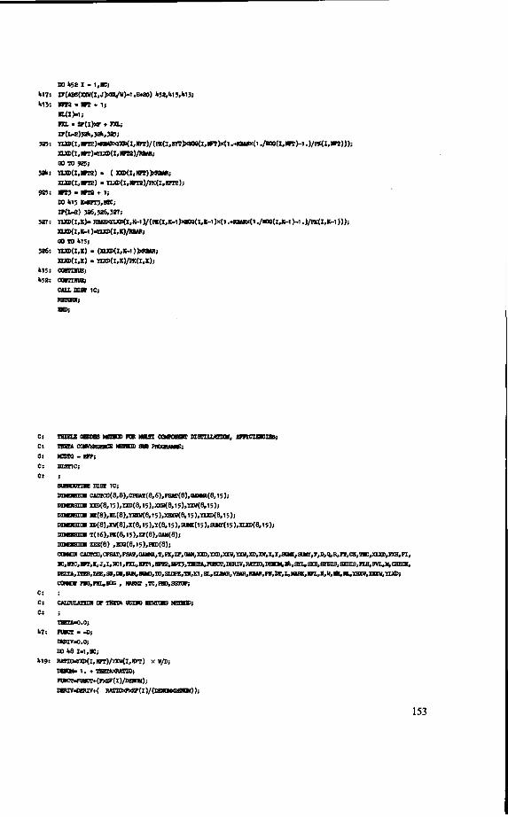
ID li52 I - 1,RC;

H 7 : XF(ABS(XXW(I,J)XEL/vM.Etao) U52,IH3,k'3;

M 3 : WT2 • R t l i

«L ( I ) - 1 ;

FXL • Zr{l)XF • R L ;

I » ( I ^ a ) 3 * , 3 * , 3 2 5 !

525: YIJOl(I,lirre)rfffl«!>COT)(I,»ri)/(EK(I,»FT)xHB(l,KraMl.-*B*Bx(l V!TO(I ,1IFTH.) /PK(I ,«PT)) ) ;

XDtD(l,10T)-YLXD(l,lffT2)/RBAR;

00 TO 925;

yk: Y u s d . a n s ) - ( xH>(i,ia»r))>4Ui»R;

XUCD(I,DT2) - nJOl(l,«FT2)/HC(l,l(PT2);

925: » T 3 - «FT2 + 1;

10 Ul5 IHDT3,1IIC;

IF(L-2) 326,526,327;

327: Y1XD(I,K)- RB*l«ILXD(l , l ! - l ) / (PK(l ,K-l)><EOO(l , l [ - l )x( l .»Ra*R)<(l . /aX)( l ,K-l ) - ' . ) /PK(l ,K-l) ) ) ;

XLXD(I,IW )-YLXD(I,lC)/RBAR;

00 TO k l5 ;

326: YLXD(I,K) • (XUO>(I,K-l))>«BARi

X L X D ( I , K ) . u s > ( i , K ) / n e ( i < i ) j

U15: CORmniE;

U52: c a m m j E ;

CALL m a r i c ;

BETUnij

c : THIKIK OBIDES ttsaui FOR HULTE coHFOsofr HianLuunaH, EFFICIENCIES;

C: TBETA CONVERGENCE MhUSUU SUB HOGRAMME;

C: MCBTQ - EFF;

C: CZST1C;

C: ;

SUBROUTHE m a r i c ;

DIMMSIOH CACTCO(8,8),CP3AT(8,6),PS*r(8),QA>»«(8,15);

DIMEHSIOS XXD(8,l5),m>(8,15),XXW(8,]5),BCV(8,15);

DIMElISiail HE(8),KL(8),mCU(8,i;),iailCV(8,13),YLXD(8,i;);

DIKEMSiaB XD(8),XW(8),X(8,15),Y(8,15)>aJMX(l5),S«t((l5),XLXI)(8,15);

I T(l6),FK(8,15),ZF(8),OAM(8);

I ZEE(8) ,HB(8 , I 5 ) ,P«D(8 ) ;

c tMOi CACTrc,CTSAT,psAT,aAM«,T,ra,z7,GAM,xro,ra,]ow,Yro,ro^

llC,HlC,HFT>K,J,I,lK1,FXI„XFri,]IFI2,liFT3,T8ETA,FUIICT,J)ERIV,]U^

I]EIU,ITER,ZEE,SS,ra,SUttSUK],TO,SU]ra,TII,K1,EL,EUAR,VBAR,RMR,PN,m^

COUCH ™o,ra.,EOo , MAHKT ,TC,PKD,SSHJP;

C: ;

C: CALCULATION OF THETA USING NEWTONS METHOD;

C: ;

THETApO.O;

l>7: FWCT • -D;

DERIV-0.0;

HO W I-1,NC;

H 9 : RATnwna>(l,RFT)/lOtV(I,HFT) X V/D;

DEHDHa T. + THEXAXRATIO;

FWCTri>WNCT+(FXZF(I)/DE«0>();

DERrVOB<IV+( RATICKF5<ZF(l)/(DE»CH<DEJO<));

153

U8: COHTIHUE;

IF (FUMCT) 60 , 50 , 61 ;

60 : FUaCM.O-rUICT;

6 1 : IF (FlmCT-1 .OE-6) 50 ,50 ,k9i

l>9: THETA*lXETA+(FlJ*Cr/DH!IV);

00 TO U7;

C: ;

C: CA1CULATI0B OF THE CORRECTED XD Aid XW FOR EACH COWCHQrT;

C: ;

50 : DO 51 1 - 1 , IE;

IF (10.(1)) 1122,1130,1122;

1(22: XD(I) « FXZF(l)/D;

XV(I) . 0 . ;

00 TO 51 ;

>>20: IF(«H(I)) U21,lt2},lt21;

k21: XD(I) • 0 . ;

XW(I) • FXZF(I)/V;

00 TO 5 1 ;

U23: RAno-Ka>(i,!OT)/rav(i ,KFT);

XD(I)*<ZF(I)/(D«KETAXWXRATIO);

x w ( i ) 4 u n a o a > ( i ) x TOETA;

5 1 : CORTDRJE;

0 : ;

c : CAicaunoH OF P L U S sauKmma A ID x AID Y FOR EACH cawararr ;

c : ;

IF(I^2) 3bO,3llO,3lH;

3k1: Bt - HFT - 1;

00 TO }h2;

3U0: n t - HPT;

3U2: s o 17 J - ' , « » ;

SUMt(J)O.0;

SUMY(J)*>.0;

Xt - 0;

DO lit 1 - 1 , K ;

fc25: IF(HH(I)) k26,li2T,U26;

kS6: X ( I , J ) - XHXV(I,J)xXW(l)>aKEtA;

Y ( I , J ) - YBXW(l,J))OCW(l)XtHBIA;

00 TO 51U;

127: Y ( I , J ) - YXD(I,J)XXD(I);

X ( I , J ) - XXD<I,J)>aS(l);

5 lU: SIKC(J)-SUME(J>riC(l,J);

1b: 3UC(J) • SUMT(J) • Y ( l , J ) ;

b53i CORHUE;

DO k;i 1-1,IK;

X ( I , J ) - X ( I , J ) /SMC(J ) ;

lt51: Y ( I , J ) . Y ( I , J ) / 6U« ( (J ) ;

I F ( * ) 22 ,17 ,22 ;

17: CQR7I1IUE;

IF(I^2) 350,350,352;

352: H- HTC-HFT +1;

00 TO 351;

350: K - n c - a r r ;

351: DO 22 »W,K;

x-ns-toi; S U K ( I ) - 0 . 0 ;

SMt(H)*>.0;

154

10 M o 1-1,«C;

i r ( IL( l ) ) l i6 l , l t6 l t , l t6 l )

i>6t i x( i ,»)^ciJCD(i,»))ca)(i)/THEm;

Y ( i , i ) - i i x i ) ( i , « ) ) on> ( i ) / r aEt» ;

00 TO W5;

fcAl X( I , I ) -DM(I ,» )>00( ( I ) ;

Y ( I , K ) - o w ( i , > ) ) o c w ( i ) ;

V65l SUCC(H). SUHK(H) + X(I ,K);

SUKffll) - SOff(H) • 1 ( 1 , 1 ) ;

M o :

* - 1;

J - I ;

00 ID k53;

CUVflRUE;

CALL m a r I D ;

REXURH;

THIELE QEIAKS MBX9DD FOR MUUFIC0MKJKJ9U1 DL9FILLATI0K, EFFICIENCIES;

CHECKS FOR COKVEROEKCE, GUZHfF SUB PfVXKttKMB;

MdnO - EFF;

mar iD;

: m a r I D ;

MKSKSiai CACTCO(8,8),CPS»T(8,6),PS»T(e),<M)»«(8,15);

DDHBIOK !03)(8,15) ,JTO(8,t5) ,XXy(8,15) ,ntW(8, l5)j

DIMBBIOK llH(8),IIL(8),YHtU(8,15),XHXV(8,15),YlXD(8,15);

DD€HSIOHXD(8),XV(8),X(8,15),*(8,15),SHC(15),S0W(15),XL}CD(8,15);

DDfE)ISIO» T(l6),HC(8,15),ZF(8),OAM(8);

DDEHSIOH ZEE(8) ,E0O(8,15),PK0(8);

COMBS CACTC0,<X>SAT,PSAT,aAIMA,T,FK,9,GiUl)CXD,XXD,)C{V,XXV,XI>,X1^X,Y,S^

IK,im:,lOT,K,J,I,lC1,PXL,IFT1,«TT2,lOT3,THffl*,yUK7r,MKIV,RATI0,DatW,lfc,Sa.,SX^^

mm,ITE«,ZEB,SS,Bl^SUH,SUMD,T0,SIiTPE,TH,lC1,EL,EiaAR,VBAR,RB»R,^^

CGMOM FKG,FXL,BOG , MARKF ,7C,PKD,SST0P;

C: i

C: CHECK FOR COHVEBOESCE OK EACH PLATE;

Ci ;

CHECKMO.O;

TO j o J-1,»TC;

I*LTA-SUMX(J)-1 . 0 ;

IF (DELIA) 62 ,30 ,63 ;

621 DELTAO.C-DELTA;

63 : IF (DELTA-U.0E-1>) 30 ,30 ,29;

2 9 ; CEBCK-CHECK+1.0;

155

50: CONTINUE;

36: IF (CHECK) 3k,3k,32;

C: OUTPUT;

3k: IF(L-2) 32,32,63k;

6311: FRiirr 103;

PRINT I Ok;

no 35 J - I , N T C ;

35: PRINT i 0 5 , J , T ( j ) , s m x ( j ) , s m f ( j ) ;

PRINT 106;

PRINT 107;

DO 27 J-1,NTC;

CO 26 1-1,IK;

666: PRINT 1 0 8 , J , I , P K ( I , J ) , X ( I , J ) , Y ( I , J ) , aAMMA(I,J),EOG(l,j);

26: CONTINUE;

27: PRINT 125;

PRINT 126, THETA;

PRINT 109,L;

U2: IF (CHECK) 37 ,37 ,32;

37: PRINT 110;

RETURN;

32 : CONTINUE;

PRINT 777;

777: F0HKAT(6HDIST2A);

CALL 0I3T 2A; C: ;

C: FORMAT STATEMENTS;

C: ;

103: FORMAT (//k5HTEMPERATURE DISTRIBUTION AND PLATE SUMMATIONS//);

10k: FORMAT (5HPLATE.11X 11BTEMPERATURE,7X 5HSUM X (S( 5HEUMY/);

105: FORMAT ( I3 ,F2k .7 ,E1k.8 ,Etk .8 ) ;

106: FORMAT (//U9HEQULLIBRIUM CONSTANT AND COMPOSITION DISTRIBUTION//);

107: FORMAT (5HPLATE,2X 9BJOMP0NE»T,TX 1HK.12X 1EX,12X 1HT,8X ;B0AHMA,8X 5H EOO / ) ;

106: FORMAT (I3,6X I3,E12.6,3X,E10.k,3X,E10.k,3X,E10.k,3X,E10.k);

109: FORMAT (/22HNUKBER OF ITERATIONS - 1 3 / / ) ;

110: FORMAT (22HCALCULATI0NS COMPLETED//);

125: FORMAT ( / ) ;

126: FORMAT (/22HTBETA -E lk . 8 ) ;

RETURN;

END;

156

C: THIELE GEDDES METHOD FUR MULTICaMPONENT DISTILLATION, EFFICIENCIES;

C: BUBBLE TEMPERATURE CALCULATIONS FOR EACH TRAY;

C: DIST2A;

C: MCDTG - EFF;

C: ;

SUBROUTINE DIST 2A;

DIMENSION CACTCO(8,8),CPSAT(8,6),PSAT(8),QAMKA(8,15);

DIMENSION XXD(6,15),YXD(8,15),XB((8,15),YXW(8,15);

DIMENSION NH(8),«L(8),YBXW(8,15),XHXH(8,15),YLXD(8,15);

DIMENSION XD(8),Xll(8),X(8,l5),Y(8,l5),SUMlC(15),SUM)r(15),]aro(8,l5);

DIMENSION T(16),FK(8,15),ZF(8),GAM(8);

DIMENSION ZEE(8) ,EOG(8,15),PKD(8);

COMMON CiraOT,CPSAT,PSAT,GAMM,T,PK,2ff,GAM,XXD,YTO,XXW,YXW,XD,XW,X,Y,SUMX,SUM^

!K,mC,KFr,K,J,I ,!K1,FXL,NIT!,NFT2,Nre3,™™,™CT,DEmV,MTIO,DEl^

DELTA, ITER,ZEE,SS,DB, SUM, SUM0,TO,SLOPE,TN,K1,EL, EXBAR,VBAR,RBAR,PN,DT,L, MARK, N ^

C0HC3K FNG,FNL,EOG , MARKT ,TC,PKD,SSTaP;

C: ;

c t CONSTRUCTION OF A NEW TEMPERATURE DISTRIBUTION;

C: USING THE BUBBLE POINT COMPUTATIONAL PROCEDURE;

C: ;

32 : DO 58 KK . l.NTC;

J • NIC + 1 - KK;

PP - 0 . ;

ITER - 1 ;

CALL ACTC;

53 : SUM-O.O;

IF (PP) 6 3 , l 6k , 63 ;

6 3 : DO 15* I-1,NC;

TC - T (J ) ;

PSAT(I)-EXP(CPSAT(I,l) • CPSAT(I,2)/(CPSAT(I,3)*TC) • CPSAT(I,lt)x TC + CPSAT(l, 5 )XTCXX2 + CPSAT(l,6)xALOG(TC));

PKD(l)-GAM(I)XPSAT(I)/PI;

15UI SUM • SUM* PKD(I) X Y ( l , l ) i

DELTA - SUM- 1 . ;

00 TO l i l t ;

16U: SUM1 - 0 .0;

IF(MARKT) 111,110,111;

111: CALL ACTC;

110: CONTINUE;

DO 5<l I-1,NC;

103: PSAT(I)rfOT(CPSAT(l,l)«PSAT(l,2)/(CPSAT(I,3)+T(j))4CFSAT(I,M>«(J)^SAT(^^^

FK(I,j)*aHHA(I,.J)xPSAT(l)/PI;

5k: CONTINUE;

IF(L-2) 112,112,113;

113: IF(J-NTC) 116,212,116;

116: DO 100 I - 1,NC;

EV • E00(I ,J ) -f ( 1 . -EOO(I ,J) )XI(I ,J*1) / (PK(I ,J)XX(I ,J) ) ;

SUM • SUM + EVXPK(I,J)XX(I,J);

100: CONTINUE;

DELTA - SUM - 1.;

00 TO 11U;

212: DO 215 1-1,NC;

215: SUM-SUMtPK(I,j)XX(l,j)xEOG(I,J);

DELTA-SUM-1.;

OOTO 11U;

112: DO 115 I - 1,NC;

SUM - SUM • PK(I,J)XX(I,J);

115: CONTINUE;

157

Ilk! 6U:

65! 55!

56i

57!

58:

62:

61 !

777!

ran* . SUM- i . i IF(MIIA) 611,58,65; DELTA-O.O-BEIXA;

I F ( D E L T A - I . O E - 5 ) 58 ,58 ,55

m ^ m - i i IF (ITER) 57,56,56; SUO-6IM; TO-T(J);

T(J)JT(J)+10.0; 00 10 53; SLBPE-(SU»-SU*»/(T(J)-TO)

TR-( (1.0-SUK)/SmPE)-tT(.j);

SUMMUK;

H > « ( J ) ;

T(JM»; X 10 53; umrruWE; IF(FP) 61,62,61; P P - I . ;

J.16; T(J) -TC; GO TO 55; PRIMP 777;

FORMAT(6HDISTIA);

7781

SUBROUFXME ACTC;

Cs SUHROUFIHE FOR THIELE- GB&EB DISTILLATION PROGRAM,;

C: CACTCO 13 A MATRIX OF BINARY INTERACTION COEFFICIENTS 10 BE USB);

c : a A VAN IAAR MULTICONPONENT Acnvrnr COEFFICIENT ESJUOION;

C: ;

Ci ;

C: MUX IS A FLU) TO IHDICATE TIE FIXST ITERATION;

C: WEN MARK IS ORE, THE ACTIVITY COEFFICIENTS THROUUBOUr THE;

Ct CQUMI ARE COMPUTED USDIQ THE COMPOSITION OF THE FEED;

C: MNtKT IS A FLU TO IHDICATE WETHER A TEMPERATURE DEPENDENCY;

C: IS INCLUDED I I THE MULTICOMPOHENT ACTIVm COEFFICIEaT B9UXI0N;

C : ;

DDOSIOH CACTCO(8,8),CF9AT(8,6),FSAT(8),(UMMA(8,15);

DIMENSION XXD(8,15),YXD(8,15),XOI(8,15),YXW(8,15);

DIMENSION IH(8),IL(8),'1[HXW(8,15),XHW(8,15),YLXD(8,15);

IX»(8) ,XV(8) ,X(8,15) ,Y(8,15) ,SIMC(l5) ,Sl»B(t5) ,XLXD(8,15);

I T(l6),FX(8,15),ZF(8),OAM(8);

I ZEE(8) ,HX)(8>15) ,FID(8);

COMB CACTC0,CF8AT,PSAT><MMNA,T,FI^ZF,0AM,XXD,YXD,XXV,YX«,XD,XV,X,Y,SU«,SU*Y,F>^^

K,ITC,Nn,KW,I,NC1,FXL,NFTl,10TC,NFT3,TIEIA,FUaCT,l>ERIV,RATI0,I>ENO^

D E U ^ TIER, ZEE, SS.IIB, SUM, S»C,T0,SLaPE,TN,K1,EI,ELB«R,VH»H,RBAR,ra,OT^

COMMOI FNG,FHL,EOO , MARKT ,TC,FKD,SSTOP;

MARKT-O;

IF(MUOC - 1 ) lK»,}O0,IU»;

300: PRmr 301;

3011 F0RMAT(/10X,2UH VAH LAAR EOLATIONS USED/);

IS ItIO X.1,NC;

SS - 0 . ;

158

i t y »

1*0!

U20!

<I10!

303!

2151

270!

2251

228:

280:

260:

250:

500:

DO U20 1-1 ,BC;

I?(OACT0O(K,I))li30,l!ltO,ll3O;

SSrfS + ZF(I) X CACTCD(l,K)/CACTCO(K,I);

00 TO *20;

SS-SS • ZT(I);

CONTINUE;

ZEE(K) - ZT(K)/SS;

CUHTIMUE;

10 250 >W,IC;

S3 - 0 . ;

KB - 0 . ;

10 260 I-l.MC;

SS - SS + CACTCO(M,I)XZEE(l);

IF(CACrCO(l,M)) 225,215,225;

10 270 K -1 ,K;

KB - SB + CACTCO(I,K)XZEE(I)xZEE(K);

00 TO 260;

10 280 E - 1 ,10;

IP (K-M) 228,280,228;

KB - DB • CACTCO(H,I)/CACTCO(I,M)xC*CTCO (I,lC)xZEE(l)xZEE(K)

OUM'IBUE;

CONmUE;

OAM(H) - EXP(SS-DB);

UUn'iWE;

Mtnc-o;

C: OHCUXB THE AUl'JLVl'rr CUEPPICTEHTS OH EACH PLATE;

C: USXHO TBE CORRECTED MILE PRACZXOBS 0? TBE LAST XTERATIOH;

C: ;

1>00: 10 210 K-1,HC;

SS - 0 . ;

DO 220 I-1.RC;

ir(CACTCO(]C, I ) )230, 2*0, 230;

230: SS-SS + X ( I ,J ) X CACTC0(I,K)/CACIC0(K,I);

00 TO 220;

2k0! SS-SS + X ( I , J ) ;

220: C0HT1HUE;

ZEE(K)«(X,J)/SS;

210: OOHTXHUE;

DO 350 )fr1,BC;

SS - 0.;

KB - 0.;

DO 360 1-1, HC;

SS . SS • CACTCOfal) X ZEE(I);

IP(C*CTCO(l,H)) 325,315,325;

315! DO 370 K-1,BC;

370: DB - DB + CACTCO(I,K)XZEE(l)XZEE(K);

00 TO 360;

325: DO 380 K-1,HC;

IT(K-M) 328,380,328;

3 2 8 : KB - OB + CACTC0(M,I ) /CACTC0(I ,M)>CACT00 ( I , X ) X Z £ E ( I ) X Z E E ( K ) ;

380: COHTHUE;

3601 COHTIHUE;

0AIMA(M,J) - EXP(SS-DB);

350: COHnHUE;

RETURH;

159

APPENDIX 5. A.

Design of bubble columns.

In the experimental apparatus, as described in Chapter 5 , bubble columns were used to obtain calibration curves and internal standardization. To make sure that complete saturation was achieved, design calculations were made.

In principle a bubble column can be designed when the ascending velocity and the diameter distribution of the bubbles are known, at least when the transfer coefficients in the liquid around a bubble (kt) and inside the bubble (kg) are known. In order to calculate reliable values for k, and kg, the gas flow-rate through the column was kept so low that the bubbles ascended chain-like or separately.

VAN KREVELEN and HOFTIJZER [98] correlated bubble diameters and ascen­ding velocities of air in water, using the Reynolds number and an 'expansion' dimensionless number (Ex). The following formula could be used for the laminar region (Re< 10) of chain like rising bubbles:

*"" = 3-22 t i ^ ) * ( ^ and for the turbulent region:

In these formulae n is viscosity, Q is the flowrate, g acceleration of gravity and Ap the difference in density between liquid and entrained gas. In FIG. 5.A. 1. these relations are sketched, for water and isopropanol at 20°C. Given the flowrate, the bubble diameter is easily calculated.

Once the diameter has been determined, the ascending velocity can be estimated from the results of GARNER and HAMMERTON [99], VAN KREVELEN

and HOFTIJZER [98] and SIEMENS and BORCHERS [100]. In F IG . 5 .A -2 a plot of asymptotic ascending velocity (v„) vs. diameter is given.

The mass transfer in a bubble column can be divided into three stages. First there is transfer during formation and release of the bubbles from the glass sinter plate (see FIG. 5.2).The second stage is the transfer during the ascent and the final stage is transfer during the residence in the foam forming at the liquid surface.

The transfer in the first stage has been subject to a considerable amount of study; the transfer efficiency is approximately proportional to the square root of the Fourier number. HEERTJES C.S. [101] suggested the correlation:

Efa = 10.3 ( f £ ) * (5A-3)

More recently a formula was proposed, HEERTJES and DE NIE [102], which requires the volume and surface of the rest-bubble to be known. In fact 5.A-3 was derived for a liquid/liquid system, one should be cautious in extrapolating

160

10°

E

10-

10"

—" Wat

jTOg* not.

L322[^r

i i ^ —

^ d = [72aV |_n2gAp

A . Iso-propanol Measurements

0.20

io- io-Q (cm 5sec- 1 )

FIG. 5.A-1. Diameter of bubbles as a function of the flowrate (Q) of gas through a sinter plate.

10"

._. Garner & Hammer ton Van Krevelen & Hoftijzer

Correlation y»=( -ar - ) M

d(cm) FIG. 5.A-2. Ascending velocity (V») as a function of bubble diameter, data of GARNER and

HAMMERTON [99], VAN KREVELEN and HOFTIJZER [88].

161

to a liquid/gas system. The time of formation (T) is approximately 0.02-0.024 sec as can be deduced from results of COPPOCK and MEIKLEJOHN [103].

Transfer during the ascent of a single bubble has been studied by numerous workers. SIDEMAN [104] gives an extensive compilation of the correlations for internal and external transfer coefficients for spherical bubbles or drops.

An important criterion in the selection of a correlation is the occurrence of internal circulation of the bubbles. A very approximate criterion for the transition of the Stokes flow pattern (rigid sphere) to the Hadamard flow pattern is the criterion of BOND and NEWTON [105].

For organic liquids this criterion predicts that down to a diameter of approxi­mately 0.2 cm internal circulation can occur. It has however been observed that small amounts of surface active substance have a strong influence on the internal circulation. DAVIS and ACRIVOS [106] derived an approximate solution to the flow pattern, culminating in a formula for the drag coefficient as a function of a surface tension group.

Owing to the liquid motion along the bubble surface, the front part of the bubble is subject to tension and the rear part is compressed. For this reason the concentration of the capillary substance adsorbed at the interface does not take the value corresponding to thermodynamic equilibrium, but a lower value at the front side and a higher value at the rear side. Thus there will be a distri­bution of surfactant over the bubble surface in such a way that the surface tension gradient balances the tangential shear stress over the surface. To use the formula of DAVIS and ACRIVOS the minimum and the maximum value of the surface tension along the surface must be known. These values however, are not easily estimated (especially the minimum value) rendering the formula less useful. On the other hand the formula predicts a sharp transition from the Stokes-to the Hadamard-region.

In the experimental apparatus the bubble size was 0.2-0.3 cm (from photo­graphic measurements). In the columns used for calibration curves and internal standardization,circulation bubbles were assumed. In the preliminary apparatus for measurements of solutions (surface activity was expected to some extent) rigid spherical bubbles were postulated in the calculations.

For non-circulation bubbles the surface- and time averaged Sherwood number in the gasphase is given by (assuming a constant surface concentration):

<S~hg> = _ | h [ ! - » ( * > ] , (5.AHI) 5 to

with the well known exact expression for $ (Fo):

<t>(Fo) = 1 - A J] X exp (- n2 n2 Fo) . (5.A-5)

* rzi n

VERMEULEN [107] showed that (5. A-5) can be replaced by:

<t> (Fo) = [1 - exp (- n2Fo) ]* . (5.A-6)

162

The liquid phase transfer coefficient can be estimated from the correlation of RANZ and MARSHALL [108]:

<Sh,> = 2 + 0.6 (Re,)* (Sc,)\ ^ > , 7 (5.A-7) ;} For bubbles with internal circulation the situation is much more complicated.

An asymptotic solution for the similar problem in liquid/liquid extraction was derived in 1949 by KRONIG and BRINK [109]. The assumption is made that the circulation time of the motion inside the bubble is short with respect to a characteristic diffusion time*. To distinguish whether this condition is met, the following relation is useful:

0.0093 g Apd3

> Ong + 2m) V1 + s/T •imi (5.A-8)

Here t, is a curvilinear coordinate (see FIG. 5.A.3) and K(f/) is the complete elliptic integral of the first kind of the argument r\. The integral is tabulated in ABRAMOWITZ and STEGUN [110, page 608]. In FIG.5.A-4 the R.H.S. of (5.A-8 ) is given as a function of £,. For air bubbles of 0.3 cm in liquids at room temperature the condition 5. A-8 is met, as can be seen from the following table:

Compound (m2/sec) Hi

(kg/msec) L.H.s.

(5.A-8)

acetone methanol

0.109 x 1<T4

0.132 x 10"* 0.34 x i r 3

0.62 x 10-3 54.7 24.7

FIG. 5.A-3. Curvilinear coordinates jj and J in which the convective diffusion equation is expressed for circulating sperical bubbles.

£1-0.00* J

* The characteristic time of diffusion is defined as the time needed to decrease the difference in average concentration with a factor e.

& . • - -

r,:-u2s —

163

A

[UA

1

^ 2 . 4

+

FIG. 5.A-4. The function of equation 5. A-8 as a function of coordinate.

Q25 0.5 Q75 1.0 I

KRONIG and BRINK showed that the R.H.S. of 5. A-8 approaches + oo as -\\rtt, in the limit <i;->-0 thus for acetone £>exp(-109.4), and for methanol £, > exp (-49.4). From figs 5.A-3 and 5.A-4 it follows that the layer at the surface of the sphere where the assumption regarding the circulation time is not valid, is extremely thin. The Kronig and Brink equation can therefore be used; for relatively short times the solution can be approximated closely using, CALDERBANK [111]:

A <I>KB (Fo) = [1 - exp (- 2.25 n2 FB) ] ' (5.A-9)

Using 5.A-9 <Shg> can be found from (5.A-4). For the liquid phase transfer coefficient the HIGHBIE approximation [112]

can be made because the velocity gradient in the contineous liquid phase at the surface of the bubble is very small. For the Sherwood number follows:

<Shi> ^ - (Pi) *(T + ?*•)* 2L 1 1 2 8 tf*>* (5.A-10) V71 \ A*i/

The transfer in the foam is very difficult to calculate. ZUIDERWEG and HARMENS [113] found that on an OLDERSHAW sieve tray, systems showing a definite tendency to foam could have an efficiency increase from 50% to 90%. However for low concentrations the foaming effect disappeared. In the present study either pure liquids or very dilute solutions (mole fractions < 10" 3) were used.

The efficiency (Murphree point efficiency) EOG can be calculated using the classical two-film theory:

EOG = 1 - exp (- Not

NOG = | <Sh„g> Fo ,

<Shog>~1 = <Shg>~

m_ dy* PMe

dx zpiRT '

i),

-' + (=£) <*>-'. (5.A-11)

164

Values for m (the slope of the equilibrium curve) are easily calculated from infinite dilution activity coefficients, for 1-butanol a value of 0.339 x 10" 2 is calculated.

For a butanol/water solution the following table was calculated:

Z)(=2R) (m)

0.008 0.004 0.003 0.002 0.001

For the

Foo (m sec"1)

0.240 0.240 0.240 0.208 0.100

liquid p

Re

(-)

19.16 9.58 7.18 2.07 0.99

tiase a diffi

NOG

(-)

0.679 1.903 2.738 4.262

20.4

H = = 0.15

EOG

(-)

0.493 0.851 0.935 0.986 0.999

m

jsion coefficient of 0.6

NOG

(-)

1.358 3.806 5.576 8.524

40.

H

x lO ' 9

EOG

(-)

0.743 0.939 0.996 0.999 1.00

= 0.30 m

m2sec~1 was assumed a viscosity of 1.0019 x 10" 3 kg m'1 sec-1 and a density of unity gives a Schmidt number (Sct) of 1670. In this table a rather low gas phase diffusion coefficient was taken: 0.2 x 10~5 m2sec~1.

For the internal standardization and calibration curve columns there is no liquid phase resistance (iVL-> - ) , the overall gas phase number of transfer units is not needed now as the efficiency now follows straight from ^^ (Fo). For a column of 0.15 m length one obtains:

D (m)

0.008 0.004 0.003 0.002

J6o (m/sec)

0.240 0.240 0.240 0.208

Fo

(-)

0.078 0.313 0.555 1.44

£ OI?

(")

0.720 0.970 0.991 0.999

FKB

(")

0.9072 0.9995 0.9999 1.0000

The apparatus of BURNETT [73] has a liquid height of 2 cm, yielding a Fourier number of 0.04 for bubbles of 2 mm, thence <Shg> = 8.25 and <Sht> = = 12.25 yielding E0G = 0.250. Admittedly the efficiency can be increased when the transfer during formation is included {E^ 0.022). The total efficiency is then given by*):

(1 - Eoa.t) = (1-3-) (1 - EOG) . (5.A-12)

A total efficiency ofEOG , = 0.27 can be estimated. The transfer in the foam will not be very large as the solutions are very diluted.

Taking a margin for the fact that the frequency distribution of the bubble diameters was not known and allowing variations in flowrates (from 0.2 x 10"6

to 1.0 x 10-6 m3 sec-1), the column for aqueous solutions was taken 50 cm and the internal standard and calibration curve columns 20 cm.

* Assuming that foam and bulk liquid have the same equilibrium concentration in vapour phase.

165

APPENDIX 5.B.

Calibration curve calculations (CALCUR).

This programme calculates calibration curves from measurements in the way indicated in section 5.2.3. The second virial coefficients of the gas mixture consisting of component i and nitrogen: Bu, BNN and the cross coefficient BlN

are calculated using the correlation of O'CONNELL and PRAUSNITZ [18, SUB­ROUTINE VIRIAL]. For the pure component virial coefficients B« and BUN:

Pcr.i Bu

Rr„ = fa (7V) + com fa (Tr) +J33(fiR, Tr) + r\i fa (7V), (5.B-1)

with Tr the reduced temperature (T/TcrJ) and nR the reduced dipole moment (105- n* • P„,i/T%r,i)> /*•• is the dipole in Debeye units. The critical pressure is in atmospheres and Tcri is in degrees Kelvin. The functions/?0 (Tr) and/?! (rr) are polynomesin l/Tr. The function fi3 (JIR, 7V)is a combination of polynomes in InfiR, while/f4 (Tr) is given by

fa (Tr) = exp [6.6(0.7 - 7V)]. (5.B-2)

The cross-virial coefficient BiN is estimated by the same relationship with mixing rules for the parameters. For the critical temperature of the mixture one can put:

Ttm = (Ttr,i-Ttr,K)i. (5.B-3)

This formula is correct for molecules of equal sizes, but predicts a somewhat too high value for TciN when the critical volumes of the two components differ widely. Eqn.(5.B-3) follows from the London theory of dispersion forces; when V„t/VcrN> 3.0 an error of about 15% may result. The acentric factor of the mixture is the arithmetic mean value of cot and coN(= 0.04) or com and coN. The critical pressure is replaced by the expression recommended by PRAUSNITZ [18]:

Per,* = 4 TciN r ^ ^ + Pcr" * H / (&.« + M * . (5.B-4)

In the expression for /iR, the factor nf is replaced by the product Qit • fiN); however, because nN = 0 , the function ^3 is deleted in the calculation of

The fugacity coefficient of the pure component i (cp?) is calculated from the formulae (compare SUBROUTINE RSTATE in ref. [18]):

In <p? = (In <p?)' + o),(ln <pf)" when 0.56 < Tr < 1.0 , (5.B-5)

and In <pf = R ^ when Tr < 0.56. (5.B-6)

The (In q>?)' and (In cp")" are functions of the reduced temperature.

166

The calibration curves of the flowrators were fitted with a power series:

Q = A! + A2F+ A3F2 + A*F3 + AsF* + A6F* , (5.B-7)

where Q is the flowrate in cm3/sec and F the flow rator reading. The constants At-A6 were obtained from a Choleski subroutine*).For flowrator (3) and (4) in fig. 5.5 six constants were used, the other were fitted with A^-A5. The accuracy of the fitting curve through experimental points is:

Flowrator RMS-error (°/0)

1 2 3 4 5

Nomenclature. CALCUR

CALIBR PHF PHIF P2VPF

A,G,C,D,E N TR TS PBAR PDELT SURFS SURFR JJJ KK F1-F5 TCRIT PCRIT VCRIT OMEGA OMEGAH DIPOLE ETA FIDENT T1-T3, V1 V3

0.975 1.568 2.320 2.420 1.568

Programme to determine calibration curves from measure­ments Sub-programme giving the output of CALCUR Arithmetic expression for (In <pf)' [5.B-5] Arithmetic expression for (In <p°)" [5.B-6] Correlation function for polar contribution to second virial coefficients (PRAUSNITZ)

Constant for eqn. 5.B-7 Number of measurements Temperature reference (°C), TR

Temperature bubble column (°C), Ts

Barometric pressure (atm) Measurement of pressure in mixing chamber ( AP, fig. 5.5) Surface area peak of component (cts), Oin

Surface area reference peak (cts), Orn

Attenuation factor for SURFS Attenuation factor for SURFR Flowrator readings (units of flowrators) Critical temperature (°A), T„. Critical pressure (atm), P„ Critical volume (cm3/mole;, V„. Acentric factor (co) Acentric factor homomorph (caH) Dipole moment (Debeye units, n() Association constant (vapour phase), t\ Identification (alphanumeric) Temperature-Molar Volume sets

' Standard SUBROUTINE of Agricultural University's Computer Centre, Wageningen.

167

CVLIQ Constants for temperature dependence of molar volumes (Cri.2, 3)

YDMIX initial estimate of v'f> mix assuming ideal vapour phase RATI01 Dilution factor 1 RATI 0 2 Dilution factor 2 VLIQ Liquid molar volume ( 1?L) SECVIR Reduced second virial coefficient (Pcri BJRTcri) RD Reduced dipole moment (10stf Pcri/T?ri) TRR Reduced temperature (TJTcri) D12 5iN in formula (5.11) PHIS Fugacity coefficient of saturated vapour (<pj") YIT Current estimate of y\ mix in iterations circuit PHI Fugacity coefficient (<p,) YMIX Mixing vapour phase mole fraction (y'{ mix) B MIX Second virial coeff. of mixture (cm 3/mole) VMIX Vapour phase molar volume (cm3/mole) FLAM Relative peak surface (Af) ALFA Linear regression coefficient.

The programme starts with reading the constants A for all the flow rators. Then it reads a title card, a card containing the number of measurements (N) and 2N cards containing measured data. The firstN cards contain the tempera­ture of the internal standard liquid, temperature of the bubble column con­taining the liquid to be measured, barometric pressure (atm), surface area of the components peak in the gas chromatogram and surface area of the internal standard peak, followed by the attenuations of the DC-amplifier of the gas-chromatograph at which the peaks were recorded. The next N cards contain 5 flow rator readings each. Finally cards are read containing data on physical properties of the component and of nitrogen: two cards with Tcr, Pcr, Vcr,a>, coH, fi (Debeye), r\ and an identification of four alphanumeric positions. The first card is for the component and the second for nitrogen. Finally a card with temperature-molar volume data for the component is read followed by a card containing the constants for the vapour pressure vs. temperature re­lation.

The programme first computes the constants for the molar volume equation (eqn.5.19) and then enters a large DO-loop in which for each data set the vapour phase mole fraction is calculated. The correlations described above are used to compute Bti, BNN, BiN and (p?, while $, y'mix, B mix and V mix are computed in an iteration loop (4 iterations are needed in general to obtain convergence with the Newton-Raphson scheme used).

Then Xin is calculated from peak area data using the equation:

Xm=jOi„/(I, kOrpIN), (5.B-8) P = i

Oin is the peak area of component 1 in the n 'th measurement, Orp the surface

168

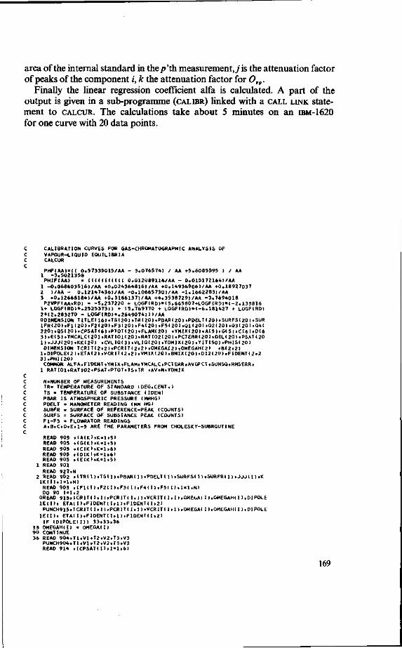
area of the internal standard in the/>'th measurement^' is the attenuation factor of peaks of the component /', k the attenuation factor for 0Tp.

Finally the linear regression coefficient alfa is calculated. A part of the output is given in a sub-programme (CALIBR) linked with a CALL LINK state­ment to CALCUR. The calculations take about 5 minutes on an IBM-1620 for one curve with 20 data points.

C CALIBRATION CURVES FOR GAS-CHROMATOGRAPHIC ANALYSIS OF C VAPOUR-LIQUID EQUILIBRIA C CALCUR C

PHF(AA>=(< 0.57335015/AA - 3.076574) / AA +5.6085595 ) / AA 1 -3.5021358 PHIFIAA) = <<((((<(<(( 0.012089114/AA - 0.015172164)/AA

1 -0.068603516)/AA +0.024364816)/AA +0.14936906)/AA +0.18927037 2 l/AA - 0.12147436)/AA -0.106657301/AA -1.16622831/AA 3 +0.12666184)/AA +0.3166137)/AA +4.3538729)/AA -3.7694018

P2VPF!AA,RDI » -5.237220 + LOGF!RD>»(5.665807+LOGFIRD)*(-2.133816 1+ LOGF(RO)*.2525373)) + (5.769770 + L0GFIRD)*(-6.181427 + LOGF(RD) 2»<2.283270 - LOGF(RO)*.2649074)I)/AA 0DIMENSION TITLEI16).TSI2OI.TR(20I.PBAR(20I.PDELT!2O),SURFS(2O)»SUR 1FR(20),F1(20>.F2(20).F3<20)»F4(20).F5<20I,Q1(20) .Q2( 20) tQ3l 20 I .Q4( 2 2 0 | i Q 5 ( 2 0 ) > C P S A T I 6 ) > P T O T ( 2 0 ) i F L A M ( 2 0 ) . Y M I X ! 2 0 1 • A ( 5 ) i G ( 5 ) > C ( 6 I » D ( 6 3 ) . E ( 5 I . Y M C A L C ( 2 0 ) , R A T I O H 2 0 > . R A T I O 2 ( 2 O ) . P C T E R R ! 2 0 ) . D E L ( 2 0 ) . P S A T ! 2 0 1 > . J J J ( 2 0 ) . K K ( 2 0 ) , C V L I Q ( 3 ) . V L I Q ( 2 0 ) . Y D M I X I 2 0 ) . Y I T ( 5 0 I , P H I S ( 2 0 1

DIMENSION T C R I T ( 2 . 2 ) . P C R I T ( 2 . 2 ) , 0 M E G A J 2 I.OMEGAH!2> , 8 ( 2 , 2 ) l . D I P O L E < 2 ) , E T A ( 2 ) , V C R I T ( 2 > 2 ) > V M I X ( 2 0 ) , B M I X ( 2 0 > > D 1 2 ( 2 0 ) , F I D E N T ( 2 > 2 3 I . P H K 2 0 )

COMMON ALFA.F IOENT , YMIX .FLAM, YMCALOPCTERR.AVGPCT.SUMSO.RMSERR. 1 R A T I 0 1 . R A T I 0 2 , P S A T . P T O T . T S > T R .AV.N .YOMIX

C C N-NUMBER OF MEASUREMENTS C TR- TEMPERATURE OF STANDARD (DEG.CENT.) C TS - TEMPERATURE OF SUBSTANCE (IDEM) C PBAR IS ATMOSPHERIC PRESSURE (MMHG) C PDELT « MANOMETER READING I MM HG) C SURFR . SURFACE OF REFERENCE-PEAK (COUNTS) C SURFS = SURFACE OF SUBSTANCE PEAK (COUNTS) C F1-F5 = FLOWRATOR READINGS

C A.B.C.D.E.1-5 ARE THE PARAMETERS FROM CHOLESKY-SUBROUTINE C

READ 905 «(A(K),K=1>5> READ 905 ,(G<K),K»1>5> READ 905 ,IC(K)»K=1.6I READ 905 ,IDCK>»K=1«6) READ 905 •(E(K>>K-1>5)

1 READ 901 READ 927.N

2 READ 902 . ( T R ! I > , T S I I ) . P B A R I I I , P D E L T ( I ) , S U R F S ( I ) » S U R F R ( I ) . J J J ( I ) , K l K ( I ) . I ' l i N )

READ 903 . ( F 1 ( I ) , F 2 ( I I , F 3 ( I I , F 4 ( I > , F 5 ( I ) , I * 1 . N ) DO 90 1 = 1 . 2

OREAD 9 1 5 . T C R 1 K I . I I . P C R I T I I , I I , V C R I T ! I . I ),OMEGA! I I .OMEGAHI D . D I P O L E I E ( I ) . E T A I I ) . F I D E N T ( I . 1 ) . F I D E N T ! I , 2 I

PUNCH915iTCRIT( I . I ) » P C R I T I I . I I . V C R I K I . I ) .OMEGA! I I .OMEGAHI I l .D IPOLE I E ( I ) . ETAI I ) . F IDENT ( I . 1 ) . F I D E N K I . 2 I

I F ( D I P O L E I I M 3 3 , 3 3 . 3 6 33 OMEGAH(I) = OMEGA!I I 9 0 CONTINUE

36 READ 904,11,VI,T2.V2.T3.V3 PUNCH904.T1.VI.T2.V2 ,T3»V3 READ 914 .(CPSATII 1,1 = 1,6)

169

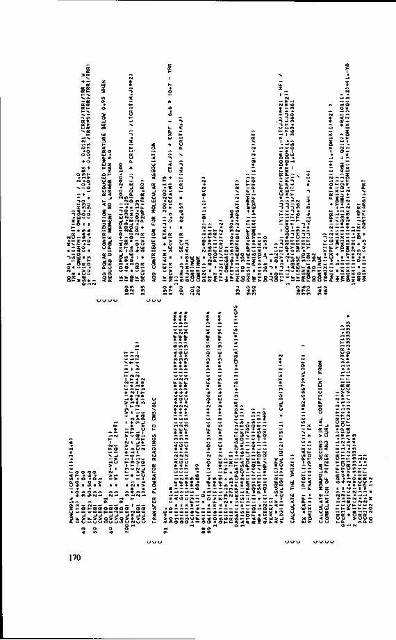
— lA a e « ( X *

o r*-• o

o o

+ o

«n + 00

o e s r -• H ^

AI » o o •

V — o

— + — + - > o " W O X m m

- < • • - > o o o • U J — » .

55, , 1-— + m * 0E • * • *

(SHJ ~ .* • • t - x »-»o

X ' • -- l o

II — < — + - . IS

- n o UJ n m

- i o a e o o n — — * (SI > 0

ae » w — o a e UJ O H * »0 * —

O —(Si

< a: o UJ • a . •* z UJ Z 1- <

X a •-UJ U Q£

a i s u i oe a <

-J

< a 0e z O t -— z t - UJ

3 ¥ o 5 Of t - UJ

§<* u a. ae a < -J o O u i a . u

Qg O UJ < ae

t_

ae u a .

o o *

o -» o — IS| UI • _l o o o a. N « i -

ma — • • T O -

a ae

ae ae

m *-m ~ . - t i i . • a — o x o > UJ (St —

_J • UJ o O J

O (SI N O .

a . o o o + «• (SIQ. o — • - o — Of * XOJ — t - * UJ 1 o si u O m • a . o - o

O o — — K

O cviae

— > o u • UJ * tO

1 V

o ae 0 £ ~

— > \j i L t a . O u . u t « « Q »

O tf> O r g *4 ^

4J LI L» KJ

— to

•n m ^

o

< U O 40 40

< ae

< - i 3 4J UI -J

i ae o u .

z o t -3 CO

ae »-z o u a a <

-> < UJ

tft + r-• X

o — o < (SI 1-• UJ

o — o * CM

lA

— O

-» — 1

< h- Of UI —

> + >J UI

— 40 X — H

< t- CC UJ —

— > u U. UI — 40

a

>. -> X

ae <j

*-* i^ m o

«M

« * ae

> — w -> UI • tO X

• CO UI UI M

-> X

X I

3 3 Z

Z O

— co m u

o «A in r» ^ *••

U W u

o o (M

o rst

Z

I—

§

(SI

(SI

CO 1

m i

(SI

CO

* (SI

n

(SI

u a (M o (S|

— (SI

— 1 - (S| to ae — H- *«. 1 -

* - -. t- ~ at <0 — u m »- H> O O v • h* —

(SIO. —

« — • y> n H-

H- 0£ K ae 0 . H>

K« ae N»

H-

< O iO •* o. <*l *

O <sj <«4 • m <M

O CO m — c\ u .

— — 0 . A I * X

(M

ISI

CO

*

— »-N- O h- t -— 0 . U, I

X u . a . a . • X X UJ + *

1- X

£5 a >•

— * u. — a. — x —

X

X — in uio ui 40 a < • * lA It — t S O — m — X UJ 1 — — a. X » - - O -O K- vO 1- tO II

* u. x o x u. -* — o-o a x

3 4*1

<•» o o •* lA i»* m

> H

>-

o lA

(SI

H

~)

r-l — O - * 1 * a ui a a • a a -H

* 1- t i - ae a : a . — . a . "» — u. -> u . a -a . X h K U J -Ui * >• * — N. — — — (SI -> ~t — «o

->"!-)« — — -> • H- f- — «0 — — t- K->- > *-• r-

— * > 9 i -r O — m

• *

•

- j

I

•* <D

* UI

T • • R

o - > x ->-> — * — L» "> i - t - 1 -

- - > a - " « — — o > > X — h- * — i 0

^.OJ — • —

H-H-

> >-O I N

-H >- IN u . u j r - » «o ui i o n I i o to t*4— «4

- as z * - > * - » « < U I m

s y - < o

— -1 — to Z X I -• O K - — T O *- — U. U. T O > •-• —

K O Q

a. u. o o « o * l * t -m r*>m

D Z

Z o

™>

> H

X

X o 4J >

4)

« (SI «0 (0

>-1

*

(SI

O

* t— ae a .

+

ae 0 ,

* (St

(SI t-l

a — * + -

x — X X

* — - = i — — > • - m * - 3 • X — (si — - v +

SIS >- * * | - (SI

.-1 — m - m * >». O (si

- * * «— * (si X — —

CO

u. 0. X UI n

X o .

< - X —

352 *?S + >-M H

• X X

X X X

CO

*

ae a . «v

IS » - o e ae < a — * u . — t-— or — o X t O

X + 03

•A + •

O (SI lA —

* * (SI • H

o —

X K O —

ae x x > co r < >

* * * * * *

<OKJ * + +

* * * * • *

I O O C

• o » c

I - (SI (SI I I - * (S»

(SI — * * ! -* • - (* * ( s i I I -— * (SI * r-« * * — > <-• * m I I - (SI

l«4 H-> I — — - * or

tsi — • -( * m _i

l — H-(Sl I _ l *

f - W X 3 I I - I —

(«4 — (SI_J

^ x 1- o

lA (Si ^ (si *•« Ci

— (h os

K O O O O O O O

* • H-

N

o o

— — — — — — Ifl •-» (M (*4 * tA — H-U. U .U. U. U. lO * * * • * * I - -— * — — — + o • » • * • * • * - » — •"

v v v w v {T| O < i S U O ui — - • + + + + + t - _J (sirsi(si ( s i ( M < — > * * * * * j> * — — 4J * * * * * o . - > — — a

- . _ „ u — — — I + H - I H — — — — — — *

H « i f l * m — h - o o i - — • * U . U . U . U, U. (M — sO + < — — * * * * * — U .1^ — iflffl to « — — — — i - O - s . — Q . O i -w n n « (n < o — — i + * _ — — W « ^ J _ J . _ — „ < o t - » o u i o . * — a — - • *M + + + + + u — — + — — — — — — — — — + - O f - — l - ( M 3 (SI(SI(M (SI ( S | n — — _l — O O "-H V w — « — « H h UI — I - — * _ l < o u o ui — at — < o <-i a . x u . > * * * o» * * - i - > - i f l a o - i * » -» — —— o — —i / j < a + — *s. I — • • H H H » _ — » _ + W) u — >. — * ~i — _ — — « » _ a + — — — - — ** ~-i r g*MA a> * t f \ « + i A U ( M - - - » ae — U . U . U . * * U, * U. H - t K - l - - U . O + + + » o o + * 4 « A « u . * < 4 A < m ae —

z « . n M . A ( 0 - - - n m a - D O i f l O 3 - l • * < , * , - « . - , » ^ — — • r - x — a n a . " i o >

. - < * - — — — — O — — — OfSIUJ — — — — + 4 J • < 0 4 j m — o * u i h - i i t o i i — + — — • — U. — H U. ( S J H — I — * - — — — > —

M H H * — II * « tt — * — ^ • f M — < — . o — - - - •* — — - — — — — — w o ^ o s * ; —

O ^ — — — <OU. — — « • - < - • — 1 - i A f - H — I * • o || w w — w W V V W H U V < H Q ) _ H I - i «* > O " ' N W U U , 4 - * O 4 M 0 K l f l l - K < l l < W > J < o o o o + " o o 4 0 i - » - Q . 4 a . a e x a e u . < >

*4 ^ t O P4

OS 00 OS

ae oe u u — > > — * —

KJ a; f~ t~ vJ —

a: oe — 3 > u o a z z o <

Q£ H- - u a c « '

o •-t - < a i o — H u. — a »-x — UJ X 1 —

* i UJ > -

I - * > o e o * o • -t0 •* (si

< < J _l 3 . UI <J ae

i g U LI

o aeoe (si * 4J4J • * » - a . -« — H H (SI —— «

w .Hoe . - - u t » - » - a •

asae + v u 1 - 0 .

u aeoe > u u o

t - o . 5

170

oe 3 KJ J

< KJ

i U.

X

< ae

8 Of a i

3 a I -

ae CQ

-J

< \J

Hi x < z o z _l -J

3 < O »-»

ae ~ < © 3 * — IM IM i f lOO— • • • * * - (M —-— < *» — O O ^ i A O h-oj N — a *M z — — u • — - . bj ifl C*> . - I f l N O U.O— o ~ * - • Of » IAN I N U . 3 a — • »/> OI3 _j * 03 — • CM • u •» » O — — — O O N o <sjm * tft v (MO — — „ - . oi — » < 0 » - N H >- — • »M «-• — a J O — — > - 1 • U N O Q : » < — o — « M « — <a o 0. i-*— U Q I U I M • O X •- <M Z — — • " U - O X o - x a x • ~ fMO>- • • - — Z — N * — i *M a a — o a — • <*» —<M >- < — (DlLO — * 0 O O. • N ( M " U l N • o o x —

- O I M raO x r y ~ _J< O — X ~ * U . CC •-• fM > aeu. • • J • * t- • — — > rg — » —o o * — CM " O N N - t * » O CM — — «*t "• M <M — i- ~4 — ae — — w o o O <J • -w i i - - - a •» »- » a i- J * o; • — • < > — u — o — ae O IM > <o M^> • » * * — CMH- o — — CM U J U . 4 N O ) - . _j » u> — CM •-. <. t - —0. u — a: H-H O U J t f U U J 1- IM * < if • - *

w — (J * — Z ^ O Z — Z <M-

a ae Ul

$ ae

i z 3 10

t -U

ft > < 0£ X ae — >

SSI t j >- - . a. • eg • z »

V * CM -J > — < < l -*-» * z X Ul >- ae a

X * U -« Ul . _Jt- — U. • -t • h- •

X O CM

X O L »->- • z • K UJ •- < a So. It o - * « (M< U. OIL • M _ |

< K < U. < »

— z N

ae ae Ul t -u a.

u - j

< u X

>-

5 -1 u. ae • ae — lu •-* to — z x ae Z K > u -a « > — < x * — o X f >

a x >- D

— «> J K O f i N O H

O l i . N > O 0 - O < * O O O ** .-• M • - • N » l l i N - H O C I/> ««n — w o _i - -z o Z O O « n - > z o —O — I I

O* Q> Q>

I X I UICM « - - ) u a . t x i - u u u u u z — — UJ - ) X ~ a •-•aeo » * • * o O H N - - Q - -

z < z z z z z -Oot 3 3 3 3 3 u o. o. a. a. a

^ 4-

to ae Z UJ O rt K ae < — i

e ui —

» < < • t 3 — ' t — O > • » — -» «) Ui • e * k « o »

CM t r ia

• X I X

S uae o o

O *H *4 ^t

• N O S U I C •U. 3 » J r> X • w»a£ • A O ul < * • r a. t ae •# r-

ae >H «\ ui ui ui • ae t - -* "V <

- U 3 - a. H-i- o

l < < ifl » X X _

„gg5 » U. U. Ul

r- o O "^

o o » - — z 4-ae a < * o z a e * - i — < •<

a o u i I O •-• — F4 « * ! U lS i ^H p-< r - z

SI ^ u. u. u. UUI

o - <

» o o

• II • • • o - —o o o n > _ • | | | | H t -

I x x >» tn a

_J<M u. * « * — — X < X Z X -> < D Z _l *0 >- U. N. + + X

z x X > z » > X x • «

^ Z Z 3 ^ ~ H D D «rt « -

— ifl «/> - • -H II H l

O X X o _ fM >- X < <*> *

SZ X U t. 5 3 J 0 3 tnt/i < a >

7 ae • u u

io

- l - Q . X 3 i . U + <v Ul rt a. i - H- — c + u u u. < 3 a. o. i-I U I O O O : - X > > o - 3 < < tO - V) « It It ae H * - • - ae K O U U K I J IO Q. a. ui - Z O >3 U7 u 3 > > z x *o < < ae

> 33 o -< ^ (M fM (*1

: 1 1 1 ^ u u \J E ZZ Z 5 3 3 3 L a. a. a

— r o

it CO

o o

» u. c> *

• • *

• CO f- U. rg • • * ^ * «M (M

• ul col­li, u » < m a: • < M l U. U

eo u3

a> ae u. •< • a

tn z • <n

to m U, N.

< O u u.

< < > Z X

g a e a e a e a e o e e e o e ^ c e a e -o o o o o oo • o o U.U-U.U.U.U-U.U,ZU.U. iMCi'4 ,>n4'>rira-co ^ o 0 0 3 O " ' ' - l ( M f M CMC*

171

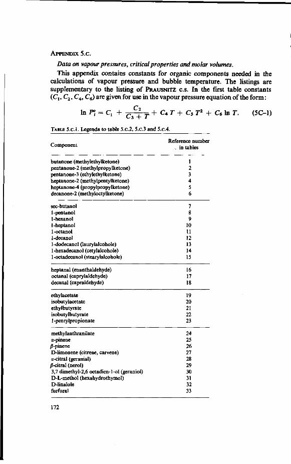
APPENDIX 5.C.

Data on vapour pressures, critical properties and molar volumes. This appendix contains constants for organic components needed in the

calculations of vapour pressure and bubble temperature. The listings are supplementary to the listing of PRAUSNITZ C.S. In the first table constants (Ci, C2, C4, C6) are given for use in the vapour pressure equation of the form:

In rt = Q + c ~ p r + CA T + Cs T* + Ce m T- (5C_1)

TABLE 5.C.I. Legenda to table 5.C.2, 5.C.3 and 5.C.4.

Reference number Component , in tables

butanone (methylethylketone) 1 pentanone-2 (methylpropylketone) 2 pentanone-3 (ethylethylketone) 3 heptanone-2 (methylpentylketone) 4 heptanone-4 (propylpropylketone) 5 decanone-2 (methyloctylketone) 6

sec-butanol 7 1-pentanol 8 1-hexanol 9 1-heptanol 10 1-octanol 11 1-decanol 12 1-dodecanol (laurylalcohole) 13 1-hexadecanol (cetylalcohole) 14 1-octadecanol (stearylalcohole) 15

heptanal (enanthaldehyde) 16 octanal (caprylaldehyde) 17 decanal (capraldehyde) 18

ethylacetate isobutylacetate ethylbutyrate isobutylbutyrate 1 -pentylpropionate

methylanthranilate a-pinene )5-pinene D-limonene (citrene, carvene) a-citral (geranial) /J-citral (nerol) 3,7 dimethyl-2,6 octadien-1-ol (geraniol) D-L-methol (hexahydrothymol) D-linalole furfural

19 20 21 22 23

24 25 26 27 28 29 30 31 32 33

172

Vapour pressure data were obtained from the Handbook of Physics and Chemistry [114], Int. Crit. Tables [60], LANDOLT-BORNSTEIN [82] and TIMMER-MANS [115]. For each component the root mean square error of the fit is given (square root of the sum of squares of deviations divided through the number of data points) as well as the temperature range covered by the data points. The constants C3 and C5 are zero for all components.

In table 5. C. 3 critical temperatures, pressures and volumes are given as well as the acentric factor (ajj) of the molecules. The data are obtained from the correlations of LYDERSEN, as they are given in SHERWOOD and REED [116]. The listing is supplementary to the listing of PRAUSNITZ c.s. [18] and O'CON-NELL and PRAUSNITZ [23].

Finally in table 5. C.4 the temperature dependence of the molar volumes of

TABLE 5.C.2. Constants for the vapour pressure equation (5.C-1)

C o m p .

1 2 3 4 5 6 7 8 9

10 11 12 13 14 15 16 17 18 19 20 21 22 23 24 25 26 27 28 29 30 31 32 33

c,

141.051969 12.7417699 45.7865513

-204.17261 82.5278676

140.940071 -132.634967

27.4251367 143.700334 525.6111437 155.712241

1529.580946 123.84396 63.152754

-123.650712 -468.632771 -491.287402

122.473049 49.494292

144.24451 130.0910853 325.9741041

-196.926603 43.1102602

140.017796 94.845778

109.970871 149.435678 136.200297 381.218470 221.425468 231.783775 258.662549

c2

-7887.08027 -^322.8782 -7137.573

559.962 -9635.2964

-10861.3616 -2673.582703 -8331.0318

-11420.7717 -25772.4003 -14250.125375 -59799.947567 -12123.333012

-9799.643476 -3767.335197

4701.439673 5545.775946

-10731.49258 -5973.734921 -8742.560874 -8653.5904

-14553.8626 -147.5386

-8333.503 -8981.390823 -7973.701856 -8595.494387

-11892.514532 -11211.724431 -20321.788695 -14228.696636 -13740.584075 -13819.8793

c«

0.030032334 -0.011204813 -0.001250264 -0.0495128

6.005946986 0.022056654

-0.054434259 -0.017258005

0.017881029 0.087490862 0.0070474366 0.29457558 0.016424604 0.005691507

-0.024586811 -0.6162398298 -0.115792429

0.018090903 0.000202266 0.02959099 0.022732364 0.075781861

-0.063562744 0.001382651 0.028308242 0.015672874 0.019478717 0.022389823 0.022063891 0.067558416 0.03809975 0.04243513 0.051867526

c.

-22.041 1.3952

^t.439 37.0

-10.26 -20.8939

27.0392 -0.011

-20.59 -83.10 -20.91

-250.6 -17.493

-7.9057 22.5392 87.00 87.00

-17.63 -5.55

-22.36 -19.592 -53.541

37.00 -4.5169

-21.6458 -13.7019 -16.301 -22.0258 -20.080 -60.2518 -34.0499 -36.1598 -41.06

Error Temp.range (RMS°lo) CA)

0.327 0.476 0.338 1.231 1.797 0.848 1.058 1.073 1.198 1.509 1.349 5.086 0.024 0.910 0.720 1.891 0.547 0.164 0.978 0.299 0.281 3.483 2.943 1.376 0.169 0.512 0.127 0.717 0.635 0.772 0.183 1.142 0.512

224-353 261-376 260-375 292-424 328-416 317^184 260-372 286-410 297-431 315-448 327-468 342-504 364-532 395-617 423-622 285-428 346-441 325-482 229-383 251-391 254-394 277-430 281^142 35(M85 272-428 277-431 287-448 334-501 334-499 342-503 329-485 313-471 291^134

173

components is given. Data were obtained from the same references as used for the vapour pressure data. Only in a few cases was more than one datum available. The molar volume is estimated from a quadratic expression when three data are available, a linear when two data are available and is kept constant when only one datum is available.

TABLE 5.C.3. Critical properties and acentric factors (Lydersen correlations) (VAPFiT-programme).

Comp.

1 2 3 4 5 6 7 8 9

10 11 12 13 14 15 16 17 18 19 20 21 22 23 24 25 26 27 28 29 30 31 32 33

T„('K)

536.91 559.91 550.91 596.0 594.65 655.49 534.65 573.95 592.07 606.69 622.70 655.10 681.37 760.04 760.04 605.58 613.47 657.99 523.25 561.15 523.25 561.15 621.95 766.54 627.78 632.62 662.94 568.21 566.43 680.71 652.09 629.87 656.87

P„(atm)

41.95 27.650 36.89 29.07 28.77 22.03 45.17 37.41 33.29 31.23 26.52 22.20 19.21 17.78 15.74 27.66 25.13 25.28 37.80 31.00 37.8 31.00 25.27 35.76 31.46 31.38 38.38 31.59 31.59 23.65 25.55 28.19 48.59

f„(cm3/mole)

277.72 455.31 314.64 412.86 429.78 558.12 233.59 295.06 336.31 357.29 429.01 515.79 616.23 723.89 768.32 454.50 472.68 507.43 297.61 376.33 297.61 376.33 517.16 426.81 428.01 431.191 365.89 196.12 192.48 552.74 478.61 411.33 289.82

(0

0.3320 0.2090 0.4280 0.5699 0.4699 0.6265 0.6311 0.7078 0.7569 0.8358 0.8542 0.9743 0.9902 1.0578 1.2136 0.4740 0.6880 0.6676 0.3624 0.4705 0.3624 0.4705 0.4366 0.5830 0.3701 0.3710 0.4106 1.9765 2.0022 0.7120 0.7808 0.8331 0.3717

174

TABLE 5.C.4. Molar volumes at different temperatures.

Comp.

1 2 3 4 5 6 7 8 9

10 11 12 13 14 15 16 17 18 19 20 21 22 23 24 25 26 27 28 29 30 31 32 33

T,{°K)

293.15 288.15 273.15 288.15 293.15 288.15 298.15 298.15 291.15 293.15 293.15 293.15 297.15 323.15 332.15 293.15 293.15 288.15 273.15 293.15 293.15 293.15 288.15 292.15 293.15 293.15 294.15 293.15 292.15 288.15 288.15 293.15 293.15

ff, (cm3/mole)

89.533 106.019 103.031 137.956 139.686 188.811 85.687

108.692 125.589 141.379 157.472 191.010 224.250 296.538 332.939 134.420 156.156 188.277 95.32

132.799 132.225 165.378 164.593 129.417 158.75 157.430 162.151 171.080 171.430 174.677 172.865 177.287 82.899

T2

— -

303.15 293.15

-295.15

------------

323.15 --

286.15 -----------

PL ril

_ -

107.045 139.055

-189.878

------------

102.026 --

165.056

-----------

T3

_ -

326.30 303.15

-303.15

------------

373.15 --------------

pL U3

_ -

109.747 139.962

-191.556

------------

110.524 -----_ ---_ _ _ _ -

175

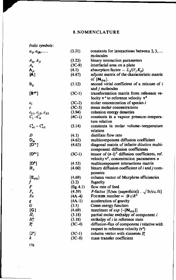
8. NOMENCLATURE

Italic symbols: aij< aijki

-^Ij' ~ t f A, A/. G*]

»U

[Bflt]

Cf

c c l l > c12> c 2 2

Q - Q

^Bl ~ Q ) 3

£) D* [D-]

[D**]

[D»] »«

{E0G} / F Fn Fo g G [G] Ht

HJ J?

{J«} k

(3.21)

(3.23) (3C-9) (4.1) (4.67)

(3.12)

(3C-1)

(3C-2) (3C-3) (3.94) (4C-1)

(5.14)

(4.1) (4.62) (4.63)

(3C-1)

(4.53) (4.60)

(4.69) (3.2) (fig.4.1) (4.59) (4A-4) (4A-1) (3.1) (4.69) (3.18) (3.18) (3C-4)

(3C-1) (3C-8)

constants for interactions between 2,3,... molecules binary interaction parameters interfacial area on a plate absorption factor = LJKVJKJD adjoint matrix of the characteristic matrix of [N o c ] . second virial coefficient of a mixture of i and j molecules transformation matrix from reference ve­locity v * to reference velocity v6

molar concentration of species i mean molar concentrations cohesion energy densities constants in a vapour pressure-tempera­ture relation constants in molar volume-temperature relation distillate flow rate multicomponent diffusion coefficient diagonal matrix of infinite dilution multi-component diffusion coefficients tensor of (n-l)2 diffusion coefficients, ref. velocity v6, concentration parameters a multicomponent interactions matrix binary diffusion coefficient of i andy com­ponents column vector of Murphree efficiencies fugacity flow rate of feed F-factor [ft/sec (superficial) . ^/lb/cu.ft] FOURIER number = 2 tjR2

acceleration of gravity GIBBS energy function matrizant of exp {-[N0G]} partial molar enthalpy of component i enthalpy of i in reference state diffusion-flux of component i relative with respect to reference velocity (v") column vector with elements J" mass transfer coefficient

176

equilibrium constant of component i on platej matrix of fc£ values matrix of k$G values multicomponent liquid phase transfer co­efficient multicomponent overall transfer coeffi­cient [cfref.20]. dimensionless parameter indicating liquid height on tray liquid phase flow rate in distillation column liquid flow rate [gal/min (average liquid flow width, ft)] characteristic length = (1/RT) da ij/dc^ slope of equilibrium curve y = mx diagonal matrix of m ̂ -values molecular weight of component i diagonal molecular weights matrix number of moles of component i unit vector perpendicular to interface total number of moles Avogadro number number of molecules of type i element of the matrix [ NOG]. overall number of transfer units when taken equal for all components number of liquid phase transfer units number of gas phase transfer units overall number of transfer units number of gas phase transfer units in bi­nary distillation of mixture i-j number of liquid phase transfer units in binary distillation of mixture i-j overall number of transfer units in binary distillation of mixture i-j reference peak surface surface element of contact area on a plate pressure Pic let number: v./?/® variable indicating thermal condition of feed to distillation column

qt (3.47) ratio of number of sites adjacent to a mole­cule of type i and the coordination number of the lattice.

Q1-Q4 (5.9) flow rates in experimental equipment (see

177

**

[ k j [k0G] *2

koG

I

L

A,

LW m [m] Mt

[M] "t

n N N Ni N& NOG

[ N J [NG] [NOG] <n •n nG

Or

dOa

p P6 q

(4.8)

(4.56) (3C-10) (-)

(-)

(3C-9)

(4.4) (4.59)

(5.5) (4A-11) (3C-18) (5.2) (3C-1) (3.11) (3C-8) (3.17) (3.47) (3.47) (4.67) (3C-26)

(4.47) (4.47) (4.47) (4.46)

(4.46)

(4.46)

(4.B-2) (4.25) (2.1) (4A-10) (-)

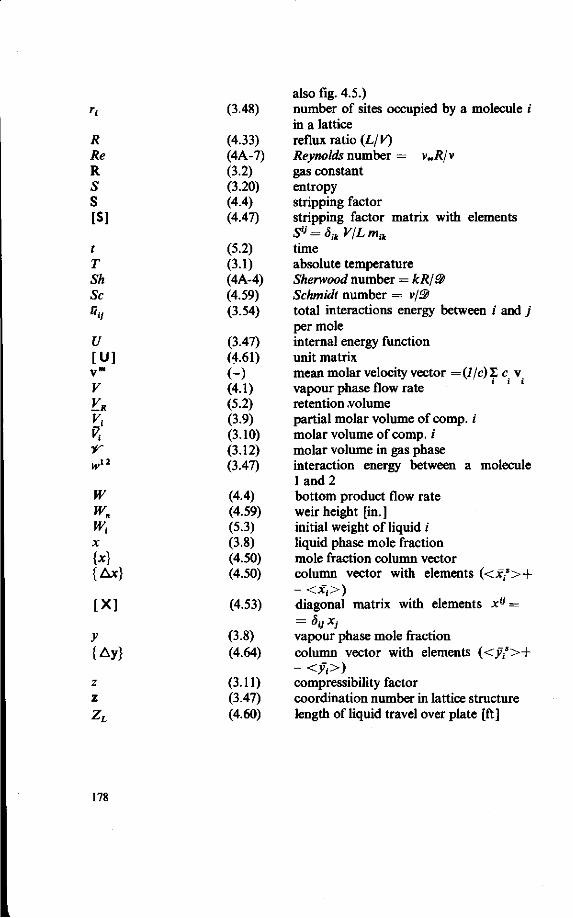
R Re R S S [S]

t T Sh Sc

%

U [U] y m

v KR

vi w12

w wn wt x W {Ax}

[ X ]

y {Ay}

z z

(3.48)

(4.33) (4A-7) (3.2) (3.20) (4.4) (4.47)

(5.2) (3.1) (4A-4) (4.59) (3.54)

(3.47) (4.61) (-) (4.1) (5.2) (3.9) (3.10) (3.12) (3.47)

(4.4) (4.59) (5.3) (3.8) (4.50) (4.50)

(4.53)

(3.8) (4.64)

(3.11) (3.47) (4.60)

also fig. 4.5.) number of sites occupied by a molecule i in a lattice reflux ratio (L/V) Reynolds number = v»/?/v gas constant entropy stripping factor stripping factor matrix with elements S« = * t tK/Lm t t

time absolute temperature Sherwood number = kR\9> Schmidt number = v/& total interactions energy between i and j per mole internal energy function unit matrix mean molar velocity vector =(7/c)S c v vapour phase flow rate retention .volume partial molar volume of comp. i molar volume of comp. i molar volume in gas phase interaction energy between a molecule land 2 bottom product flow rate weir height [in.] initial weight of liquid i liquid phase mole fraction mole fraction column vector column vector with elements (<xl

s>+ ~ <*i>) diagonal matrix with elements x,J = = dijxj

vapour phase mole fraction column vector with elements (<y'>+ - <y~i>) compressibility factor coordination number in lattice structure length of liquid travel over plate [ft]

178

Greek symbols:

aiw (2.1)

Pi

f«

rl0, ri, r

l (o

8

0(7}) OE(TJ)

K

A,

h

V-i

«5

P

T

(5.15) (2.1)

(3.58)

(5.5) (5.11)

(3.67) (5.A-8)

(-) (5.2)

(4.19) (4.44)

(5.2) (5.15)

(3.36)

(3.37) (5.A-1) (-) (3.41)

(3.36) (5.A-8)

(3.91)

(3.92)

(5.A-1) (3.42)

(5.A-3) (3.6)

relative volatility of component / with respect to water regression coefficient relating yt to k{

activity coefficient of component i in the liquid phase Interaction parameter for a binary system of/andj surface excess parameter related to second virial coeffi­cients parameters related to Ty parameters curvilinear coordinate for circulation flow in bubbles or drops association factor of a component i convergence parameter for distillation computer programmes bubble temperature function for plate j function for determination of 7} when efficiencies are included integration dummy variable ratio between peak surfaces in gas chro-matograms ..interaction energy" parameter between molecules i and./ Wilson parameters viscosity dipole moment of molecule type i relative frequention of contribution Xk t o

activity coefficient at infinite dilution „local" volume fraction of component i curvilinear coordinate for circulation flow in bubbles or drops complex expression in /1-parameter equations for activity coefficients complex expression for multicomponent systems appearing in /1-equations mass density parameters in correlation for infinite dilution coefficients proposed by Helpin-still and Van Winkle contact time vapour phase fugacity coefficient of com­ponent i in a mixture

179

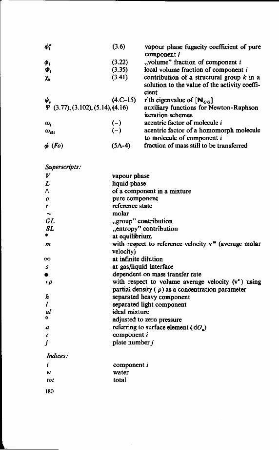
<t>!

Xk

*r (4-C-15) «P (3.77), (3.102), (5.14), (4.16)

CO,

CO Hi

<f>(Fo)

(3.6) vapour phase fugacity coefficient of pure component /

(3.22) „volume" fraction of component i (3.35) local volume fraction of component i (3.41) contribution of a structural group A: in a

solution to the value of the activity coeffi­cient r'th eigenvalue of [NOG] auxiliary functions for Newton-Raphson iteration schemes

(-) acentric factor of molecule i (-) acentric factor of a homomorph molecule

to molecule of component i (5A-4) fraction of mass still to be transferred

Superscripts: V L A 0

r f>*

GL SL * m

oo s • •P

h I id 0

a i J

Indices:

i w tot

vapour phase liquid phase of a component in a mixture pure component reference state molar „group" contribution „entropy" contribution at equilibrium with respect to reference velocity vm (average molar velocity) at infinite dilution at gas/liquid interface dependent on mass transfer rate with respect to volume average velocity (v") using partial density ( p) as a concentration parameter separated heavy component separated light component ideal mixture adjusted to zero pressure referring to surface element (dOa) component i plate number j

component i water total

180

/ feed plate location ca calculated co corrected F in feed W in waste product from reboiler D in distillate j plate number or component j H separated heavy components L separated light components exp experimental ext external mix after mixing cm critical mixing

at infinite dilution c condensor OG overall gas phase cl difference between successive plates b bubble loc local s interfacial e vapour entering plate o vapour leaving plate lam laminar turb turbulent /, L liquid phase g, G gas phase r reduced cr critical

Mathematical and thermodynamical operators: A a finite difference Det {A], I A | determinant of the square matrix [A] Gj partial molar property (G) of component i, G must

represent any extensive quantity of a system A G excess function of G e AJJJG change in G-function on mixing

8^ Kronecker delta {a} • {b} dot-product of the vectors {a} and {b} {a} {b} „dyadic" product of the vectors {a} and {b} *) V Nabla operator A characteristic function of a matrix

* The analogy between the product {a} {b} as used in the text and the true dyadic product of two vectors in three dimensional space is only formal.

181

erfc (x) complementary error function of argument x <xt> surface averaged value of xt : A~l f (xt dA

_ _ i f ' + i l

xt time smoothed value of xt : At J xtdt, no con­fusion with the partial molar property notation should arise because xt is an intensive property

[Xi] volume averaged value of liquid mole fraction leaving a plate: c^LT'CC xfvd„ dOd

where Od is the area of a cross section of the down-comer

[U] unit matrix {1} unit column vector

182

PREFERENCES

1. THIJSSEN H. A. C , Middelberg L.R.W.A., Report I.I.F.-I.I.R., Commission 6B, Delft, 30th Aug-1 Sept (1966).

2. MILLEVILLE H. P. and ESKEW R. K., USDA, Bur. Agr. and Ind. Chem. AIC-63 (1944, suppl. 1945).

3. CLAFFEY J. B., ESKEW R. K., EISENHARDT N. H., Aceto N.C., USDA, ARS-73-19 (1958). 4. ROGER N. F., TURKOT V. V., Food Technology 19, 69-72, Jan (1965). 5. NAWAR W. W., Food Technology 20, 115-117, Febr. (1966). 6. WIENTJES A. G., Jnl. of Food Sri. 33 (1), 1-2, (1967). 7. THIJSSEN H. A. C , RULKENS W. H., De Ingenieur 80 (47), Ch45-56, (1968). 8. HOLLAND C. D., Multicomponent Distillation, Prentice Hall, Englewood Cliffs N.J.

(1964). 9. WEURMAN C , Report R16-78, CIVO, Zeist, The Netherlands, April 1968.

10. NURSTEN H. E., WILLIAMS A.A., Chemistry and Industry, 486-497, March 1967. 11. DUPAIGNE P., Fruits 14 (3), 127-141, (1958). 12. GIERSCHNER K., BAUMANN G., in Solms J., Neukom H., Aroma- und Geschmackstoffe

in Lebensmitteln; 4-5 april 1967 course E.T.H., Forster Verlag Zurich, Switzerland, (1967).

13. PERRY J. H. ed., Chemical Engineers' Handbook, 4th Ed., Mc Graw Hill, (1963). 14. CARLSON H. C , COLBURN A. P., Ind. Eng. Chem. 34, 581-589 (1942). 15. HILL T. L., An introduction to Statistical Thermodynamics, Adisson-Wesley, Reading

(Mas) (1960). 16. GUGGENHEIM E. A., Mixtures, Clarendon Press, London (1952). 17. ORYE R. V., Ph-D Thesis in Chem. Eng., Chemical Engineering Dept., University of

California, Berkeley (1965). 18. PRAUSNITZ J. M., ECKERT C. A., ORYE R. V., O'CONNELL J. P., Computer calculations

for multicomponent Vapour Liquid Equilibria, Prentice Hall, Englewood Cliffs, N.J. (1967).

19. CAPATO A. J., Chem. Eng. Dept., Columbia University, IBM 1620 Program Library No. 9.3.012.

20. DIENER D. A., Gerster J. A., Ind. Eng. Chem. Fundamentals 7 (3), 339-345, (1968). 21. VAN NESS H. C , Classical Thermodynamics of non-electrolyte solutions, Pergamon

Press, Oxford, (1964). 22. PITZER K. S., CURL R. F., J. Am. Chem. Soc. 79,2369-2370, (1957). 23. O'CONNELL J. P., PRAUSNITZ J. M., Ind. Eng. Chem. 6 (2), 245-250, (1967). 24. SCATCHARD G., Trans. Far. Soc. 33, 160-166 (1937). 25. IBL W. V., DODGE B. F., Chem. Eng. Sri., 2,120-126, (1953). 26. WOHL K., Trans. Am. Inst. Chem. Engrs. 42, 215-249 (1946). 27. REDLICH O., KISTER A. T., Ind. Eng. Chem. 40, 345-348, (1948). 28. WILSON G. M., J. Am. Chem. Soc. 84,127-133, (1964). 29. WILSON G. M., Scatchard G., J. Am. Chem. Soc. 84,133-137, (1964). 30. HILDEBRAND J. H., SCOTT R. L., Solubility of non-electrolytes, 3rd Ed., Dover Publ.,

New York, (1946). 31. GUGGENHEIM E. A., Proc. Roy. Soc. A, 183, 203-212, (1944). 32. GUGGENHEIM E. A., Proc. Roy. Soc. A, 183,213-227, (1944). 33. GUGGENHEIM E. A., Fowler R., Statistical Thermodynamics, Cambridge Univ. Press,

(1939). 34. BROWN G. M., SMILEY H. M., Am. Inst. Chem. Eng., J. 12 (3), 609-610, (1966). 35. SCATCHARD G., HAMER W. J., J. Am. Chem. Soc. 57,1085, (1935). 36. NAGEL O., SINN R., Chem. Ing. Techn. 39 (11), 671-676, 275-282, (1967). 37. NAGEL O., SINN R., Chem. Ing. Techn. 38 (10), 265, (1966). 38. ORYE R. V., PRAUSNITZ J. M., Ind. Eng. Chem. 57 (5), 19-26, (1956).

183

J

39. PIEROTTI G. J., DEAL C. H., DERR E. L., Ind. Eng. Chem. 51, (1), 95-102, (1959). 40. DEAL C. H., DERR E. L., Ind. Eng. Chem. 60 (4), 28-38 (1968). 41. WILSON G. M., DEAL C. H., Ind. Eng. Chem. Fund. 1, (1), 20-23, (1962). 42. SCHELLER W. A., Ind. Eng. Chem. Fund., 4, 459-462, (1965). 43. HELPINSTILL J. G., VAN WINKLE M., Ind. Eng. Chem., Proc. Des. and Dev. 7 (2), 213-

220, (1968). 44. PRIGOGINE I., DEFAY R., Chemical Thermodynamics (translated by D. H. Everett),

Longmans and Green, London, 3rd Ed., (1965). 45. KORN G. A., KORN T. M., Mathematical Handbook 13.5.6, page 372, Mc.Graw Hill,

New York, (1961). 46. GUGGENHEIM E. A., Thermodynamics, North Holland Publ. 5th rev. Ed., (1967). 47. PRAUSNITZ J. M., SHAIN S. A., chem. Eng. Sci. 18, 244-246 (1963). 48. COPP J. L., EVERETT D. H., Disc. Far. Soc. 15, 268, (1953). 49. HUGGINS M., Ann. New York Ac. Sc. XLHI, Art. 1, 1-32 (1942). 50. FLORY P. J., J. Chem. Phys. 10, 51-61, (1942). 51. WEIMER R. F., PRAUSNITZ J. M., Hydrocarbon Process. Petrol. Refiner, 44, 237, (1965) 52. UCHIDA S., KATO H. J. (see Perry, 13), J. Soc. Chem, Ind. (Japan) 37, 525, (1934). 53. MARQUARDT D. W., Chem. Eng. Progress., 55 (6), 65-70, (1959). 54. CAREY J. S., LEWIS W. K., Ind Eng. Chem. 24,882-883 (1932). 55. NOYES, WARFLE., J. Am. Chem. Soc. 23,463 (1901). 56. STOCKHARDT J. S., HULL C. M., Ind Eng. Chem. 23, 1438-1440, (1931). 57. ALTSEEBEEVA A. I., BELOUSOV V. P., OVTRAKHT N.V., MORACHEVSKII A. G., Russ.,

Inl. Phys. Chem. 38 (5), 676-678, (1964). 58. OTHMER D. F., CHUDGAR M. M., LEVY S. L., Ind. Eng. Chem. 44 (8) 1872-1878, (1952). 59. MARSHALL N., J. Chem. Soc. 89, 1350, (1906). 60. International Critical Tables, Mc Graw-Hill, New York, (1928). 61. THIELE E. W., GEDDES R. L., Ind. Eng. Chem. 25 (3), 289-295, (1933). 62. GARNER F. H., ELLIS S. R. M., PEARCE C. J., Chem. Eng. Sci. 3, 48-54 (1954). 63. WILKE C. R., Chem. Eng. Progress, 45, 218-224, (1949). 64. WILKE G R., CHANG D., Am. Inst. Chem. Engrs. J., 1 (2), 264-270, (1955). 65. WILKE C. R., LEE C. Y., Ind. Eng. Chem., 47, 1253, (1955). 66. GILLILAND E. R., ROBINSON C. S., Elements of Fractional Distillation, Mc.Graw Hill

4th Ed., New York,.(1950). 67. KwANTES A., RIJNDERS G. W. A., Gas Chromatography, Butterworths, (1958). 68. DESTY D. H., GOLDUP A. Gas Chromatography, R. P. W. Scott (ed.), Butterworths,

(1960), p. 162. 69. HOFSTEE T.,KwANTES A., RIJNDERS G. W. A., Int. Symp. on Distillation (Inst, of Petro­

leum) (1960). 70. KEULEMANS A. I. M., Gas Chromatography (ed. Veryer), Reinhold, chapt. 7 (1957). 71. EVERETT D. H., STODDART C. T. H., Trans. Farad. Soc., 57, 746-754 (1961). 72. EVERETT D. H., Trans. Farad. Soc., 61,1637-1645 (1965). 73. BURNETT M. G., Anal. Chem. 35 (11), 1567-1570, (1963). 74. BARKER C. A. P., VAN BUYTENEN P. M., BEEK W. J., Chem. Eng. Sci. 21, 1039-1046,

(1966). 75. STEPHEN H., STEPHEN T., Solubilities of In-Organic and Organic compounds, Pergamon

Press, New York, (1963). 76. DANCKWERTS P. V., Chem. Eng. Sci., 2, 1-12 (1953). 77. MEIGH D. F., CURRAH I. E., J. Sci. Fd. Agric, 17, 428-433, (1966). 78. WEURMAN C , Food Technology, 15, 231, (1961). 79. MCWILLIAM I. G., J. Chromatog. 9,110-117, (1960). 80. KEPNER R. E., MAARSE H., STRATING J., Anal. Chem., 36 (1), 77-82, (1964). 81. MAHADEVAN V., STENROOS L., Anal. Chem., 39 (13), 1652-1654, (1967). 82. LANDOLT-BORNSTEIN, Physicochemische Tabellen, 6° Auflage, (1955). 83. HALA E., PICK J., FRIED V., VILIM O., Vapour Liquid Equilibrium (translated by G.

Standart), Pergamon Press, (1958).

184

84. GARNER F. H., ELUS S. R. M., PEARCE C. J., Chem. Eng. Sci., 4, 273 (1955). 85. GRISWOLD J., BUFORD C. B., Ind. Eng. Chem., 41, 2347, (1949). 86. PICK J., FRIED V., HALA E., VIIJM O., Chem. Lysty, 47,1750, (1953). 87. CARLSON C. S., SMITH P. V., MORELL C. E., Ind. Eng. Chem., 46 (2), 350-365, (1954). 88. BONAUOURI E., CARPANI Z., DALL'ORTO D., Chim. e Industr., 38, 768, (1956). 89. GRISWOLD J., CHU P. L., WINDSAUR W. O., Ind. Eng. Chem., 41 (10), 2352-2358, (1949). 90. SAMADAR S. P., NANDI S. K., Trans. Indian Inst. Chem. Engrs., 26,1218, (1934). 91. JANECKE E., Z. Phys. Chem., 194, 207, (1950). 92. GRISWOLD J., DIMVIDDIE J. A., Ind. Eng. Chem., 34, 1188, (1942). 93. FORDYCE C. R., SIMONSE D. R., Ind. Eng. Chem. 41 (1), 104-106, (1949). 94. DE GROOT S. R., MAZUR P., Non-equilibrium Thermodynamics, North Holland Publ.,

(1962). 95. BIRD R. B., STEWART W. E., LIGHTFOOT E. N., Transport Phenomena, Wiley, New

York, (1965). 96. HIRSCHFELDER J. O., CURTISS C. F., BIRD R. B., Molecular Theory of Gases and Liquids,

page 718, Wiley, New York, (1954). 97. FRASER R. A., DUNCAN W. J., COLLAR A. R., Elementary Matrices, Cambridge Univ.

Press, (1965). 98. VAN KREVELEN D. W., HOFTUZER P. J., Chem. Eng. Progress, 46 (1), 29-35, (1950). 99. GARNER F. H., HAMMERTON D., Chem. Eng. Sci., 3 (1), (1954).

100. SIEMENS W., BORCHERS E., Chem. Eng. Sci., 12 (2), 77-87, (1960). 101. HEERTJES P. M. c.s., Chem. Eng. Sci., 3, 122 (1954). 102. HEERTJES P. M., DE NIE L. H., Chem. Eng. Sci. 21, 755-768, (1966). 103. COPPOCK P. D., MEIKLEJOHN G. T., Trans. Inst. Chem. Engrs. (London) 29, 75, (1951). 104. SIDEMAN P., in: Advances in Chemical Engineering, Academic Press (1966). 105. BOND N. W., NEWTON D. A., Phil. Mag. 75, 794, (1928). 106. DAVIS R. E., ACRIVOS A., Chem. Eng. Sci. 21, 681-685, (1966). 107. VERMEULEN TH., Ind. Eng. Chem. 45, 1664, (1953). 108. RANZ W. E., MARSHALL W. R., Chem. Eng. Progress 48, 141-146,173-180, (1952). 109. KRONIG R., BRINK J. C , Appl. Sci. Res. A2, 142-154, (1950). 110. ABRAMOWITZ M., STEGUN, IRENE A., Handbook of Mathematical Functions, Dover,

(1965). 111. CALDERBANK P. H., KORCHINSKI I. J. O., Chem. Eng. Sci. 6, 65, (1956). 112. HIGHBIE R., Trans. Am. Inst. Chem. Engrs., 31, 365-389, (1935). 113. ZUIDERWEG F. J., HARMENS A., Chem. Eng. Sci. 9, 89-103, (1958). 114. WEAST R. C , SELBY S. M., HODGMAN C. D., Handbook of Physics and Chemistry, 45th

Ed., Chem. Rubber Co., Cleveland (Oh.), (1964). 115. TIMMERMANS J., Physico Chemical Constants of Pure Organic Compounds, Elsevier,

A'dam, (1950). 116. REID R. C , SHERWOOD T. K., Properties of Gases and Liquids, McGraw-Hill, New

York, (1958).

185