ACTUARIAL RESEARCH CLEARING HOUSE 1991 VOL. 1

OPTION BOUNDS IN DISCRETE TIME WITH TRANSACTION COSTS

by

Phelim P. Boyle*

and

Ton Vorst**

July 1990

Revised August 1990

* Professor of Finance and Actuarial Science, School of Accountancy, University of Waterloo, Waterloo, Ontario, Canada N2L 3G1

** Professor of Mathematical Economics, Econometric Institute, Erasmus University Rotterdam, P.O. Box 1738, DR 3000 Rotterdam, The Netherlands

The authors are grateful to Antoon Pelsser, Jeroen de Munnik, Lijiang Fang, and Ruth Comale for research assistance, and to Philippe Artzer, Giovanni Barone-Adesi, Fischer Black, John E. Gilster Jr., D. C. Heath, and Eric Reiner for helpful suggestions. PPB acknowledges research support from Erasmus University Rotterdam, the J. Page R. Wadsworth Chair at the University of Waterloo, and the Natural Scitnces and Engineering Research Council of Canada.

3 6 5

OPTION BOUNDS IN DISCRETE TIME WITH TRANSACTION COSTS

by

Phelim P. Boyle

and

Ton Vorst

ABSTRACT

Option bounds are obtained in a discrete-time framework with transaction costs. The model

represents an extension of ,,~e Cox-Ross-Rubinstein binomial option pricing model to cover the

case of proportional transaction costs. The method proceeds by constructing the appropriate

replicating portfolio at each trading interval. Numerical values of these bounds are presented for

a range of parameter values.

366

OPTION BOUNDS IN DISCRETE TIME WITH TRANSACTION COSTS

1. INTRODUCTION

The classic Black-Scholes option pricing model rests on perfect market assumptions. A

replicating portfolio can be constructed consisting of a long position in the risky asset and a short

position in bonds which is equal in value to the price of a call option. As time passes, the

weights of this portfolio are rebalanced so that it replicates the pay-off of the option contract at

maturity. Under perfect market assumptions this rebalancing is costless, but if we introduce

transaction costs this is no longer the case. It is of interest to explore the implications for option

pricing and option replication of the introduction of tr.ansaction costs. Our paper explores this

issue in a discrete-time setting.

The first paper to relax the assumption of no transaction costs in the context of option pricing

was by Gilster and Lee [1984]. These authors also incorporated differential borrowing and

lending rates in their analysis. Their basic model was developed using a continuous time

framework but to circumvent the problem of infinite transaction costs they used discrete time

rebalancing in their hedge construction.

Leland [1985] also examined this problem in a continuous-time framework. He obtained a

367

modified Black-Scholes formula and develops an alternative replicating strategy to incorporate

the impact of transaction costs. The Black-Scholes formula is modified by increasing the

variance by a factor which depends on the magnitude of the uansaction costs. Under his

alternative replicating strategy the pay-off on the portfolio at option expiration approximates the

maturity value of the call option. Leland notes the difficulty of incorporating transaction costs

in a continuous-time framework and he uses periodic portfolio revisions for his numerical

simulations.

An alternative and more convenient approach is to embed the problem in a true discrete-time

framework. Merton [1990] uses this approach to explore the impact of transaction costs on

option prices in a two-period binomial model. He assumes that the upper bounds for the option

value is equal to the value of a replicating ponfc ,~ which has the same value at expiration as

the option. The portfolio revisions at the intermediate trading date allow for transaction costs.

Menon uses this approach to determine the production cost to a financial intermediar3' of

manufacturing a call option and _-xamines the relationship between the bid-ask spreads in the

option market to the size of the transaction costs in the market for the underlying asset.

Our approach is similar to Merton [1990] but we extend the analysis to an arbitrary number of

periods whereas Merton's model just involved two periods. We employ the discrete time

framework of Cox, Ross, and Rubinstein [1979] and obtain upper and lower bounds for the

European call price in this framework. The upper bound is obtained by finding the cost of

replicating a long position in the option by a dynamic hedging strategy. Proportional transaction

3 6 8

costs are incurred at each revision date upon either the purchase or the sale of shares of the risky

asset. The lower bound is obtained, in a similar way, by finding the cost of replicating a short

position in the option. If there were no transaction costs the (absolute) value of these two

portfolios would be equal. The impact of transaction costs is to drive a wedge between these two

values: the higher the transaction costs the wider the wedge.

These bounds stem from no-arbitrage arguments. If an investor can create a long synthetic call

more cheaply than she can purchase a comparable call in the market, an arbitrage opportunity

exists. Hence, the current value of the replicating portfolio (for the long call) provides an upper

bound for the call price. In the same way, the (absolute) value of the replicating portfolio that

precisely duplicates the maturity payoff to a short call position provides a lower bound for the

call price.

We begin with a single period model and indicate how to obtain the upper bound in this case.

This one period model is then extended to several periods and we develop a recursive procedure

to obtain the replicating portfolio for the upper bound. The procedure for obtaining the lower

bound is similar but not identical. The zero-transaction costs option values lie between the lower

bound and the upper bound, as we would expect. Furthermore, as the transaction costs tend to

zero, the bounds converge to the Cox-Ross-Rubinstein option prices. We are able to derive a

compact, closed-form expression for the option upper bound when the number of trading intervals

is large. In this case, the option upper bound can be approximated by the ordinary Black-Scholes

formula with an adjusted variance. Our variance adjustment is similar to, but larger than, that

369

derived by Leland [1985] in his paper on transaction costs.

Shen [1990] also employs a discrete-time framework to examine the impact of transaction costs

on option prices and obtains upper and lower bounds. His conclusions are similar to ours but

there are distinct differences between the two approaches. Our approach differs from Shen's in

that we derive a Black-Scholes-type approximation for the value of the replicating portfolio with

transaction costs. In addition, we focus on some technical differences between the construction

of the upper and lower bounds. On the other hand, Shen covers several issues that we do not

address. These include a discussion of two types of settlements (cash or stock), option pricing

by a risk averse dealer, and optimization of the number of trading dates in a fixed time interval.

Hence, the two papers complement one another.

Other authors have recently explored the impact of transaction costs on option prices in different

settings. Hodges and Neuberger [1989] assume a continuous-time framework and derive bounds

on option prices by assuming a particular utility function for the intermediary (or individual)

creating the hedge. Figlewski [1989] uses simulation techniques to examine the impact of

transaction costs on option prices and concludes that

"transaction costs for the standard arbitrage trade, induce arbitrage bounds around

the theoretical option values that are substantially wider than the bid-ask spreads

observed in practice."

Biais and Hi]lion [1990] derive a model for the bid-ask spread in option prices using a market

micro-structure approach.

370

The layout of the present paper is as follows. In Section 2 we derive the upper bound for the

one-period case and indicate how to extend the approach to many periods. In Section 3 we

derive an analytical expression for the option upper bound in the presence of transaction costs.

Section 4 develops some convenient approximations and derives a closed form Black-Scholes-

type expression for the upper bound. In Section 5 we demonstrate how the lower bound for the

option price can be derived. We explore the numerical properties of these bounds in Section 6.

Section 7 concludes the paper.

2. O P T I O N R E P L I C A T I O N IN D I S C R E T E T I M E W I T H T R A N S A C T I O N C O S T S

In this section we use no-arbitrage a x aments to establish the cost of creating a long European

call option by dynamic hedging when there are transaction costs. This furnishes an upper bound

for the call price. In the two-period case our model reduces to that obtained by Merton [ I990]

when allowance is made for differences in notation and convention? We use the multiplicative

binomial lattice employed by Cox, Ross, and Rubinstein [1979] for the asset price

~Our notation differs from Merton's and we make different assumptions concerning the transaction costs incurred at the outset and in the final period.

371

Su

Su 2

S Sud

Sd

Sd2

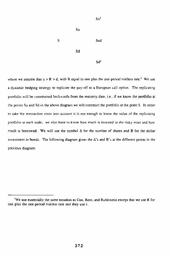
where we assume that u > R > d, with R equal to one plus the one-period riskless rate? We use

a dynamic hedging strategy to replicate the pay-off to a European call option. The replicating

portfolio will be constructed backwards from the maturity date, i.e., if we know the portfolio at

the points Su and Sd in the above diagram we will construct the portfolio at the point S. In order

to take the transaction costs into account it is not enough to know the value of the replicating

portfolio at each node; we also have to know how much is invested in the risky asset and how

much is borrowed. We will use the symbol A for the number of shares and B for the dollar

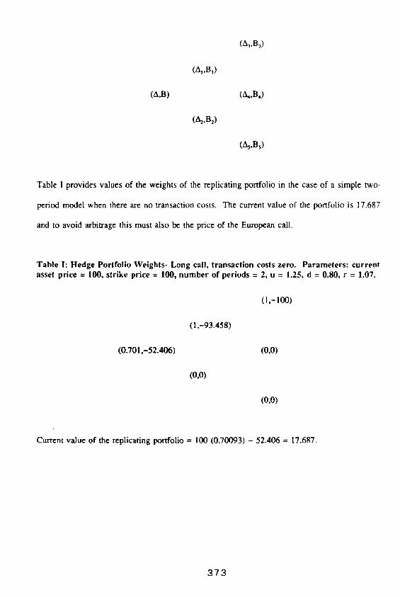
investment in bonds. The following diagram gives the A's and B's at the different points in the

previous diagram:

2We use essentially the same notation as Cox, Ross, and Rubinstein except that we use R for one plus the one-period riskless rate and they use r.

372

(AI,BI)

(~,B~)

(A,B) (A,,B,)

(A2,B2)

(As,B~)

Table I provides values of the weights of the replicating portfolio in the case of a simple two-

period model when there are no transaction costs. The current value of the portfolio is 17.687

and to avoid arbitrage this must also be the price of the European call.

Table I: Hedge Portfolio Weights- Long call, transaction costs zero. Parameters: current asset price = 100, strike price = 100, number of periods = 2 , u = 1 . 2 5 , d = 0 . 8 0 , r = 1 . 0 7 .

(I,-93.458)

(0.701,-52.406) (0,0)

(0,0)

( l , - l O 0 )

(0,0)

Current value of the replicating polxfolio = I00 (0.70093) - 52.406 = 17.687.

373

To introduce transaction costs, assume that proportional transaction costs are incurred when

shares of the risky asset are t raded? Let k be the transaction costs measured as a fraction of the

amount traded. We must select A and B so that the portfolio (A~,B~) can be bought if the up-

state Su occurs and (A2,B2) can be bought if the down-state Sd occurs. This leads to the

fol lowing two equations:

ASu + BR - A1Su + B I ÷ klA - AIISu (1)

ASd + BR - A2Sd + B 2 + klA - AalSd. ~2)

Equation (1) indicates that the value of the portfolio in the up-state is exactly enough to buy the

appropriate replicating portfolio corresponding to this state and to cover the transaction costs

incurred in the rebalancing. Equation (2) has a similar-interpretation for the down-state. Since

we don ' t know whether the risky asset has to be bought or sold, but in both cases transaction

costs have to be paid, we use the absolute value of A - A~ and A - A 2. Equations (1) and (2)

are two nonl inear equations in A and B, and it is not obvious whether a solution exists, and, if

a solution exists, whether it is unique. However, in the appendix we prove the fol lowing result.

3Proportional transaction costs on bonds can also be incorporated. However, the model becomes much more complicated without providing new insights.

3 7 4

T h e o r e m 1. In the construction of a synthetic long European call option by dynamic hedging,

equations (1) and (2) have a unique solution (A,B). Furthermore, for this solution the following

inequality holds

A 2 -< A -< A l . (3 )

This theorem enables us to rewrite equations (1) and (2) in the following form

ASu + BR - AISu + B t + k(A 1 - A)Su (4)

or equiva]ently,

ASd + BR - ~ S d + B2 + k(A - A2)Sd,

AS5 + BR - A,S5 ÷ B,

(5)

(6)

where

ASd + BR - AzSd + B2, (7)

- u ( l + k) and d - d ( l - k). (8)

3 7 5

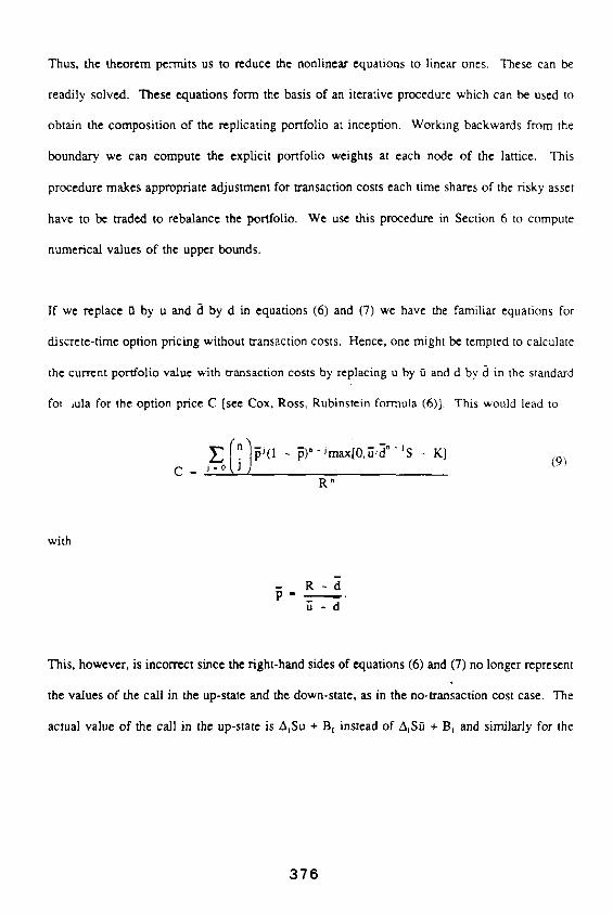
Thus, the theorem permits us to reduce the nonlinear equations to linear ones. These can be

readily solved. These equations form the basis of an iterative procedure which can be used to

obtain the composition of the replicating portfolio at inception. Working backwards from the

boundary we can compute the explicit portfolio weights at each node of the lattice. This

procedure makes appropriate adjustment for transaction costs each time shares of the risky asset

have to be traded to rebalance the portfolio. We use this procedure in Section 6 to compute

numerical values of the upper bounds.

If we replace ia by u and d by d in equations (6) and (7) we have the familiar equations for

discrete-time option pricing without transaction costs. Hence, one might be tempted to calculate

the current portfolio value with transaction costs by replacing u by fi and d by a in the standard

fol ,ula for the option price C [see Cox, Ross, Rubinstein formula (6)]. This would lead to

C ° R*

(9)

with

This, however, is incorrect since the right-hand sides of equations (6) and (7) no longer represent

the values of the call in the up-state and the down-state, as in the no-transaction cost case. The

actual value of the call in the up-state is AISu + B t instead of AtS~ + B 1 and similarly for the

376

down-state.

Our equations (4) and (5) provide the basis for the recursive approach to determine the portfolio

weights at intermediate trading dates in the presence of transaction costs. Apart from notational

differences, they correspond to equation (14.2c) in Merton [1990]. We assume that the institution

(or intermediary) creating the replicating portfolio does not have to buy the initial amount of the

risky asset (A). Hence, we just take account of the additional transaction costs necessary to

maintain the replicating portfolio. In our numerical examples we assume that the replicating

portfolio at option expiration for an in-the-money call option consigts of one unit of the risky

asset and a short position in riskless bonds equal to the exercise price. Our conventions

correspond to those employed by Leland [1985] rather than those used by Merton [1990]."

We can rework our earlier two-period example to illustrate the impact of transaction costs. Table

II provides the portfolio weights required to create a long (synthetic) call option when k = 0.01.

Note that the holdings of the risky asset are higher in Table 11 than in Table I. The current value

of the replicating portfolio of 18.307 represents the upper bound.

'Merton assumes that the entity constructing the replicating portfolio pays the necessary transaction costs to establish the initial asset position and also that the asset holdings in the replicating portfolio are liquidated at expiration.

377

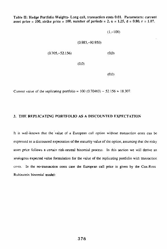
Table II: Hedge Portfolio Weights- Long call, transaction costs 0.01. Parameters: current asset price = 100, s t r i k e p r i c e = 100, n u m b e r o f periods -- 2, u = 1.25, d = 0 .80, r = 1.07.

(0.983,-90.950)

(0.705,-52.156) (0,0)

(0,0)

(1,-100)

(0,0)

Current value of the replicating portfolio = I00 (0.70463) - 52.156 = 18.307.

3. THE REPLICATING PORTFOLIO AS A DISCOUNTED EXPECTATION

It is well-known that the value of a European call option without transaction costs can be

expressed as a discounted expectation of the maturity value of the option, assuming that the risky

asset price follows a certain risk-neutral binomial process. In this section we will derive an

analogous expected value formulation for the value of the replicating portfolio with transaction

costs. In the no-u'ansaction costs case the European call price is given by the Cox-Ross-

Rubinstein binomial model:

3 7 8

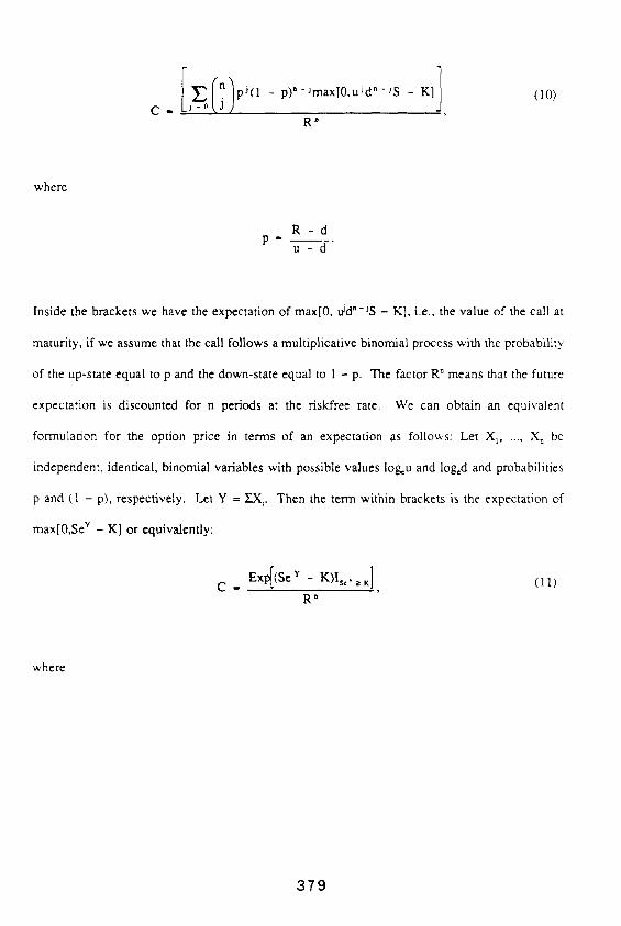
C -

p) '~-Jmax[0,uJd"-)S - K]]

R"

(10)

where

p - ~ _ . R - d

u - d

Inside the brackets we have the expectation of max[0, u)d"-)S - K], i.e., the value of the call at

maturity, if we assume that the call follows a multiplicative binomial process with the probability

of the up-state equal to p and the down-state equal to 1 - p. The factor R" means that the future

expectation is discounted for n periods at the riskfree rate. We can obtain an equivalent

formulation for the option price in terms of an expectation as follows: Let X~ . . . . . X, be

independent, identical, binomial variables with possible values log~u and log,d and probabilities

p and (1 - p), respectively. Let Y = .Y.X,. Then the term within brackets is the expectation of

max[0,Se "~ - K] or equivalently:

C - Exp[(SeV- K)Is"~K] ( l l ) R o

where

379

ISe) >K

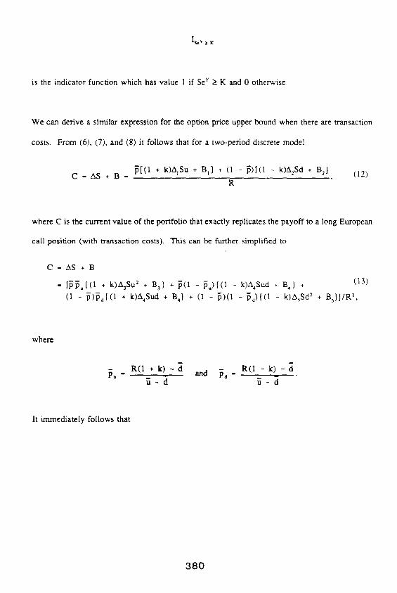
is the indicator function which has value 1 if Se v >_ K and 0 otherwise.

We can derive a similar expression for the option price upper bound when there are transaction

costs. From (6), (7), and (8) it follows that for a two-period discrete model

C - AS + B - ~ [ ( I + k)A)Su + Bz] + (I - ~ ) [ ( I - k)A~Sd + B2] (12)

R

where C is the current value of the portfolio that exactly replicates the payoff to a long European

call posiuon (with transaction costs). This can be further simplified to

C-AS +B

= [~.{(i + k)~Su 2 + B 3} + ~(I - ~.)1(I - k)A, Sud + B,) + (13)

( 1 - p ) p d { ( 1 + k)A4Sud + B,} + (1 - 5 ) (1 - ~d){(1 - k)AsSd2 + Bs}] /R 2,

w h e r e

R(! + k ) -

~ - d and ~ , =

R ( I - k ) -

~ - ~

It immediately follows that

380

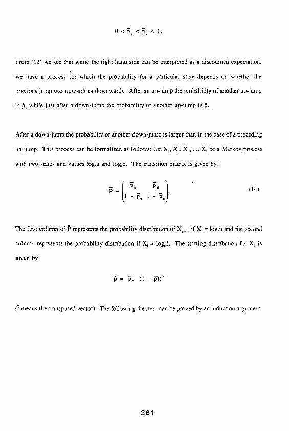
0<~,<~< 1.

From (13) we see that while the right-hand side can be interpreted as a discounted expectation,

we have a process for which the probability for a particular state depends on whether the

previous jump was upwards or downwards. After an up-jump the probability of another up-jump

is ~ while just after a down-jump the probability of another up-jump is 13~.

After a down-jump the probability of another down-jump is larger than in the case of a preceding

up-jump. This process can be formalized as follows: Let X~, X> X 3 ..... X~ be a Markov process

with two states and values log~u and log,& The transition matrix is given by:

(14~

The first column of P represents the probability distribution of Xj .~ ~ if Xj = logeu and the second

column represents the probability distribution if Xj = log, d. The starting distribution for X, is

given by

- ~ , ( l - ~ ) ~

(: means the transposed vector). The following theorem can be proved by an induction argument.

381

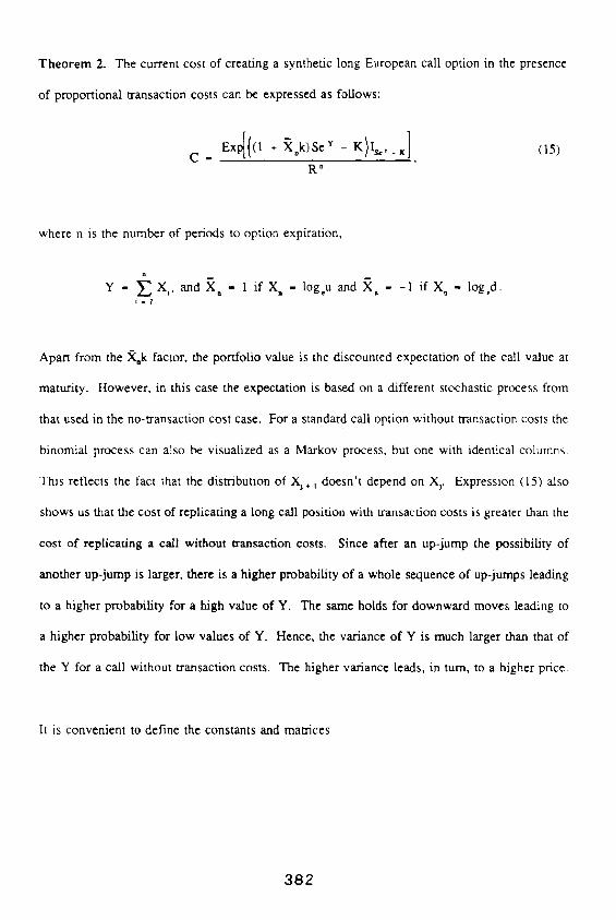
Theorem 2. The current cost of creating a synthetic long European call option in the presence

of proportional transaction costs can be expressed as follows:

C - Exp[((1 + X k)Se v - K ) I s , , _ x ] (15)

R °

where n is the number of periods to option expiration,

Y - ~ X,, and X, - 1 if X, - log u and X - -1 if X, - log d. l - |

Apart from the ~ factor, the portfolio value is the discounted expectation of the call value at

maturity. However, in this case the expectation is based on a different stochastic process from

that used in the no-transaction cost case. For a standard call option without transaction costs the

binomial process can also be visualized as a Markov process, but one with identical columns.

This reflects the fact that the distribution of Xj . t doesn't depend on Xj. Expression (15) also

shows us that the cost of replicating a long call position with transaction costs is greater than the

cost of replicating a call without transaction costs. Since after an up-jump the possibility of

another up-jump is larger, there is a higher probability of a whole sequence of up-jumps leading

to a higher probability for a high value of Y. The same holds for downward moves leading to

a higher probability for low values of Y. Hence, the variance of Y is much larger than that of

the Y for a call without transaction costs. The higher variance leads, in turn, to a higher price.

It is convenient to define the constants and matrices

382

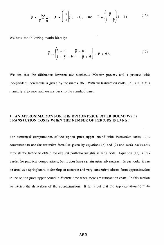
I'l 0 - Rk A - (1, - I ) , and P - (1, 1). ~ - a ' -~ 1 -~

(16)

We have the following matrix identity:

~ - e 1 " 1 - ~ + 8 P + O A .

(17)

We see that the difference between our stochastic Markov process and a process with

independent increments is given by the matrix OA. With no transaction costs, i.e., k = O, this

matrix is also zero and we are back to the standard case.

4 . AN APPROXIMATION FOR THE OPTION PRICE UPPER BOUND WITH TRANSACTION COSTS WHEN THE NUMBER OF PERIODS IS LARGE

For numerical computations of the option price upper bound with transaction costs, it is

convenient to use the recursive formulae given by equations (6) and (7) and work backwards

through the lattice to obtain the explicit portfolio weights at each node. Equation (15) is less

useful for practical computations, but it does have certain other advantages. In particular it can

be used as a springboard to develop an accurate and very convenient closed-form approximation

to the option price upper bound in discrete time when there are transaction costs. In this section

we sketch the derivation of the approximation. It turns out that the approximation formula

383

corresponds to the Black-Scholes formula with an adjusted variance.

To develop this value for large n, we f'n'st have to define a binomial tree. We will use the

standard binomial tree as in Cox and Rubinstein [1985] with parameters s u, d, and R given by

u - e a':b, d - e -*'~', R - e r~ (18)

where h = T/n, o is the volatility of the risky asset, and r is the riskless continuous interest rate.

We assume that the t ime to maturity of the option, T, is exactly one year.

In deriving the approximation formula it is necessary to make some approximations. However,

we will show in the next section that the approximation formula is very, accurate for the

parameter values that are likely to be of interest.

If we consider the Markov process described in the previous section, we have the following

result.

L e m m a 1. The variance of the random variable Y of Theorem 2 has the following behaviour

for large n and small k

~Clearly the parameters u, d, and R depend on n. We suppress this dependence for convenience.

384

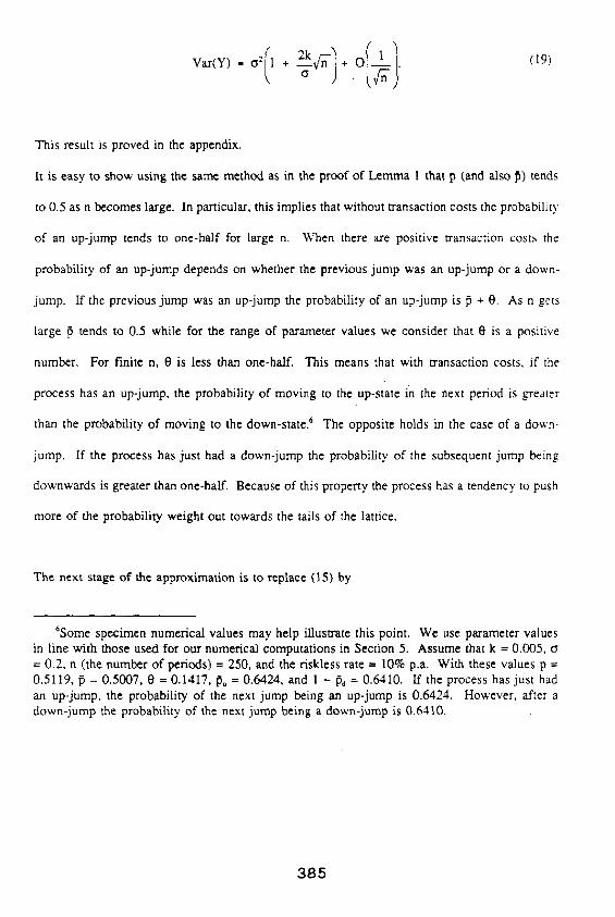
V a t ( Y ) - a : 1 + --~-v/-n "- +. "~'n " (19)

This result is proved in the appendix.

It is easy to show using the same method as in the proof of Lemma 1 that p (and also ~) tends

to 0.5 as n becomes large. In particular, this implies that without transaction costs the probability

of an up-jump tends to one-half for large n. When there are positive transaction costs the

probability of an up-jump depends on whether the previous jump was an up-jump or a down-

jump. If the previous jump was an up-jump the probability of an up-jump is } * 0. As n gets

large ~ tends to 0.5 while for the range of parameter values we consider that O is a positive

number. For finite n, 0 is less than one-half. This means that with transaction costs, if the

process has an up-jump, the probability of moving to the up-state in the next period is greater

than the probability of moving to the down-state. 6 The opposite holds in the case of a down-

jump. If the process has just had a down-jump the probability of the subsequent jump being

downwards is greater than one-half. Because of this property the process has a tendency to push

more of the probability weight out towards the tails of the lattice.

The next stage of the approximation is to replace (15) by

6Some specimen numerical values may help illustrate this point. We use parameter values in line with those used for our numerical computations in Section 5. Assume that k = 0.005, = 0.2, n (the number of periods) = 250, and the riskless rate = 10% p.a. With these values p = 0.5119, ~ = 0.5007, 0 = 0.1417, Pu = 0.6424, and 1 - Pd = 0.6410. If the process has just had an up-jump, the probability of the next jump being an up-jump is 0.6424. However, after a down-jump the probability of the next jump being a down-jump is 0.6410.

385

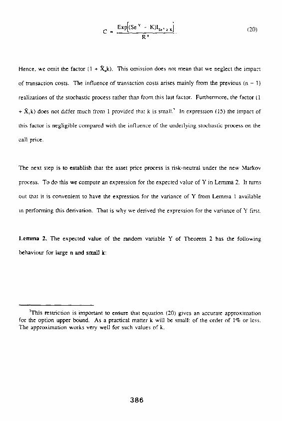
C - Exp[(SeV- K)ls"~K] (20)

R"

Hence, we omit the factor (1 + )~k). This omission does not mean that we neglect the impact

of transaction costs. The influence of transaction costs arises mainly from the previous (n - i)

realizations of the stochastic process rather than from this last factor. Furthermore, the factor (1

+ X,k) does not differ much from 1 provided that k is small. ~ In expression (15) the impact of

this factor is negligible compared with the influence of the underlying stochastic process on the

call price.

The next step is to establish that the asset price process is risk-neutral under the new Markov

process. To do this we compute an expression for the expected value of Y in Lemma 2. It turns

out that it is convenient to have the expression for the variance of Y from Lemma 1 available

in performing this derivation. That is why we derived the expression for the variance of Y first.

Lemma 2. The expected value of the random variable Y of Theorem 2 has the following

behaviour for large n and small k:

"This restriction is !mportant to ensure that equation (20) gives an accurate approximation for the option upper bound. As a practical matter k will be small: of the order of 1% or less. The approximation works very well for such values of k.

386

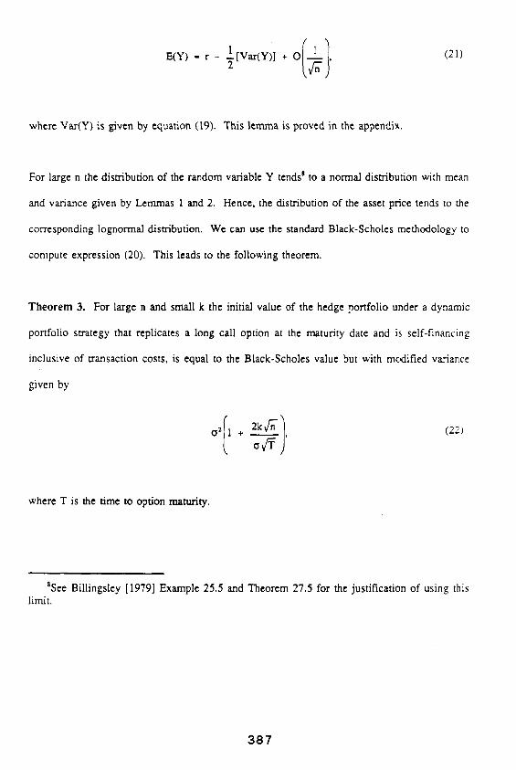
E(Y) - r - l [ v a r ( Y ) ] + O I , (21)

where Var(Y) is given by equation (19). This lemma is proved in the appendix.

For large n the distribution of the random variable Y tends B to a normal distribution with mean

and variance given by Lerrtmas 1 and 2. Hence, the distribution of the asset price tends to the

corresponding lognormal distribution. We can use the standard Black-Scholes methodology to

compute expression (20). This leads to the following theorem.

Theorem 3. For large n and small k the initial value of the hedge portfolio under a dynamic

portfolio strategy that replicates a long call option at the maturity date and is self-financing

inclusive of transaction costs, is equal to the Black-Scholes value but with modified variance

given by

o:f)' (22)

where T is the time to option maturity.

~See Billingsley [1979] Example 25.5 and Theorem 27.5 for the justification of using this limit.

387

Theorem 3 provides a very convenient method to compute the upper bound. As noted above we

will illustrate the accuracy of the approximation formula in Section 6. We can compare our

formula with that of Leland. In Leland's approach the dynamic portfolio strategy is not self-

financing since he uses a continuous model with discrete revision times. Leland also derives a

Black-Scholes-type formula with modified variance. The two expressions for the variance are

very similar, but where Leland has a factor of ",/(2/~) we have unity. Since ",/(2/~) = 0.8, our

model leads to higher option values than Leland's. This is to be expected since our discrete

model involves no residual hedging errors.

In the analysis thus far we have concentrated on dynamic hedging strategies that exactly replicate

the payoff to a long position in a European call option. The current value of the replicating

pc folio represents the cost of creating a synthetic option with the same terminal value to an

economic agent facing proportional transaction costs k. As such, it provides an upper bound for

the option price. We now examine the lower bound.

5. LOWER BOUNDS FOR THE OPTION PRICE

In this section we explore the derivation of a lower bound for the option price in a discrete-time

model when there are proportional transaction costs. 9 To obtain the lower bound we compute

the cost of creating a self-financing replicating portfolio which has exactly the same value at

9 We are grateful to Fischer Black for suggesting we examine this issue.

388

expiration as a short position in a European call. The dynamic hedging slrategy takes account

of the transaction costs incurred at each trading date. The intuition corresponds closely with that

behind the derivation of the upper bound, However, there are some important technical

differences.

First consider a one-period model. Note that if we are replicating a short position in a call option

the replicating portfolio at expiration will consist of a short position in the asset plus a long

position in the risky asset (or else zero shares of each security). If the call is in the money at

expiration the value the replicating portfolio at expiration will be negative. The replicating

portfolio at the start of the period also involves a short position in the risky security.

We assume the same notation as in Section 2 and derive some arbitrage bounds that will be

useful in the sequel. Assume an investor purchases one share of the risky asset at the start of

the period and sells it at the end of the period. The initial amount required is S(l+k) and if the

up-state occurs the net proceeds upon sale arc Su(1-k). If the initial amount were invested in

the riskless asset the proceeds would be SR(I+k). Since the maximum return from the risky

strategy must exceed the risk]ess return we have

u(1 - k) > R(1 * k). (23)

In the same way if we consider the short sale of the risky asset we obtain:

389

R(1 + k) > d( l + k). (24)

From these two equations we note that

u(1 - k) > d(1 + k). (25)

Now the recursive equations for the replicating portfolio which has a payoff equal to the short

position in the call option are exactly the same equations as (1) and (2). One difference is that

the sign of the holdings in the risky asset is now negative (or zero) on the boundary.

Corresponding to Theorem 1 we have

T h e o r e m 4. In the const, .ction of a synthetic short call position by dynamic hedging there is

a unique solution to equations (1) and (2) provided that equation (25) is satisfied,

The proof is given in the Appendix. It is insmacdve to compare this result with Theorem 1 for

the long call position. There are some important differences. First, note that we require equation

(25) to hold for Theorem 4 to be valid. No such requirement was needed to prove Theorem 1.

Hence, we would expect Theorem 1 to be valid for a wider range of parameter values than the

present theorem. We will f'md this to be the case in Section 6. Second, in the present case the

number of shares of the risky asset at successive nodes on the expiration boundary satisfy

390

Aj. 1 > A j,

where Aj is the number of shares at node j and ~ . I is the number of shares at the node (j + 1)

just below it. The asset price at node j is higher than the asset price at node (.j + 1). It is not

necessarily the case that the number of shares to be held one period earlier at the node from

which both j and (j + I) can be accessed lies in the interval [z~,Aj,. i]. This contrasts with the

situation in Theorem 1 where the number of shares held at a given node always lay in the

interval spanned by the number of shares held at the two adjacent nodes one period later.

However, we can still compute the numerical values of the risky asset and bond holdings at each

node to replicate the maturity payoff to a short call option. This is again accomplished by

solving equations (1) and (2) recursivley. There are two changes with the earlier case. First, the

boundary, values will be exactly the negative of those for the long call position. Second, we have

to be more careful at each step of the iteration to ensure we have obtained the correct holdings

of the risky asset at each node in the correct region. We know from Theorem 4 that there is a

unique solution but we cannot guarantee that it is in the region spanned by the holdings at the

two adjacent next-period nodes. It is easy adapt our numerical algorithm to ensure that we have

the correct solution in the appropriate region.

As noted earlier the current value of the replicating portfolio that generates the synthetic short

call position provides (the negative of) a lower bound for the call option price. We provide some

numerical estimates of the lower bounds obtained in this way in the next section. We also know

391

that the value of a European call cannot be less than the difference between the current asset

price and the present value of the strike price (or zero if this expression is negative). We can

use this lower bound for those parameter values for which the approach suggested here breaks

down.

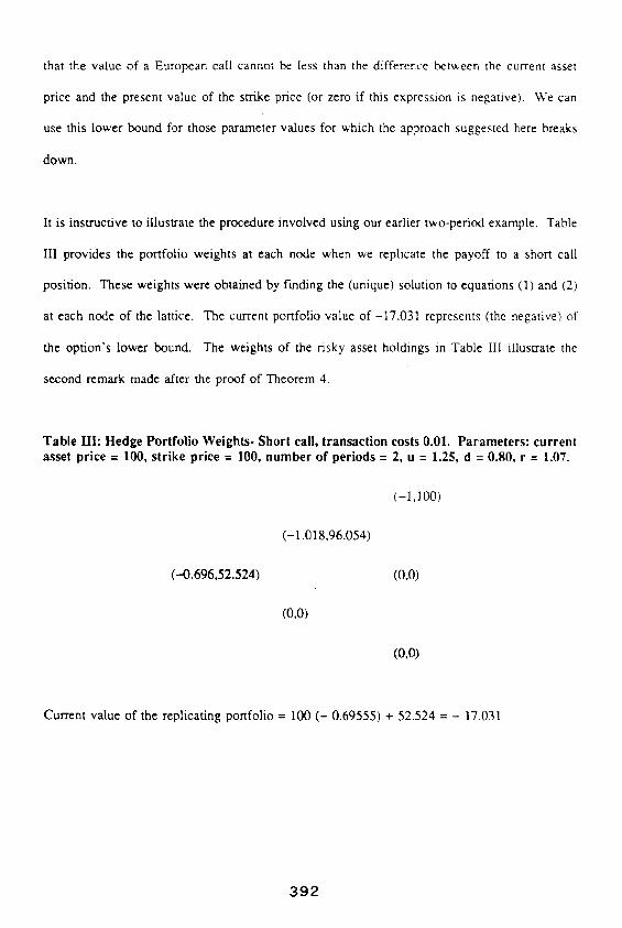
It is instructive to illustrate the procedure involved using our earlier two-period example. Table

III provides the portfolio weights at each node when we replicate the payoff to a short call

position. These weights were obtained by f-mding the (unique) solution to equations (1) and (2)

at each node of the lattice. The current portfolio value of - I7 .031 represents (the negative) of

the option's lower bound. The weights of the risky asset holdings in Table III illustrate the

second remark made after the proof of Theorem 4.

Table HI: H e d g e Port fo l io Weights - Short call, transact ion costs 0.01. Parameters : current asset price = 100, s tr ike price = 100, n u m b e r of periods = 2, u = 1.25, d = 0.80, r = 1.07.

(-1.018,96.054)

(--0.696,52.524) (0,0)

(0,0)

(-1,100)

(0,0)

Current value of the replicating portfolio = 100 ( - 0.69555) + 52.524 = - 17.031

392

In the case of the upper bound we were able to develop a compact expression for the long call

and ultimately a Black-Scholes-t)pe approximation to its value. In the present case the nature

of the result in Theorem 4 suggests that we cannot write down an algebraic expression for the

value of the lower bound corresponding to equation (15). The problem arises because the

number of shares of the risky asset, t~, sometimes lies within the interval [At,~.z] and sometimes

outside this interval. The portfolio weights in Table III illustrate this behaviour. In the topmost

mangle, -1.018 lies outside the interval [-1,0], whereas the asset portfolio weights for the other

nodes lie within their appropriate intervals.

If we could assume that A alway~ lay within the interval [At,th] then equations (1) and (2) for

the lower bound would be structurally the same as equations (6) and (7) for the upper bound

except that -: replaces k. Were this the case, we could develop the analogue of (15) by

replacing k with -k. This in turn would justify a Black-Seholes-type approximation for the lower

bound with the variance given by equation (22) with -k replacing k. This procedure of replacing

k by -k and using the corresponding formula for the upper bound produces answers that are

often quite close ~° to the accurate lower bounds even though the procedure lacks a rigorous

justification.

~0 We investigated the accuracy of the lower bound results obtained by this procedure by comparing them with the accurate values obtained from solving (1) and (2) recursivley. The agreement was generally very good. To conserve space we do not report the detailed results here.

393

6. N U M E R I C A L C A L C U L A T I O N S

In this section we compute option price bounds for a range of parameter values. It In addition

to il lustrating the comparat ive statics, n These computat ions form a basis for comparison with

the approximation we introduced earlier. For all our simulations we take the current price of the

risky asset to be 1(30, the time to option expiry one year, and the (effective) t~ interest rate to

be 10% p.a. For our base case assumptions the standard deviation of the return on the risky asset

is 20% p.a. We examine the impact on the option bounds of variations in the strike price and

of variations in the transaction costs. The zero transaction cost case corresponds to the Cox-

Ross-Rubinstein case and is used as a benchmark.

Our approach is to present the results for the upper bound case first. " able IV provides the

option upper bounds for a range of transaction cost and strike price assumptions. The first panel,

corresponding to k = 0, contains the zero-transaction cost benchmark prices. The impact of

transaction costs on the upper bound is most transparent if we subtract these reference prices

from the option upper bounds. These differences are tabulated in Table IVa. As we would

expect the influence of the transaction costs increases with the frequency of trading and also with

the magni tude of the costs. As the swike price increases, the size of the upper bound spread

" O u r parameter values correspond to those assumed by Leland.

t: Many of the comparat ive statics for the upper bound case were also observ Leland(1985).

~3 This means that one dollar invested for one year at the riskless rate accumulates to $1.10.

394

increases, reaches a maximum, and then decreases. The upper bound spread is highest when the

current asset price is equal to the discounted strike price. This corresponds to the case when the

option's time value is highest. In a discrete-time model we can see the intuition behind this

result. Consider a call which is very deep in the money so that there is no chance TM it will

mature out of the money. The dynamic replicating portfolio in this case is certain to consist of

a long position in the underlying asset and a short position in the discounted strike price. If this

portfolio is maintained throughout the lattice there will be no transactions required. At the other

extreme, consider an option which is so far out of the money that there is zero chance that it will

end up in the money. In this case the option value at expiration will be zero so that the hedge

portfolio is degenerate consisting of no risky asset and no bonds. To maintain such a portfolio

throughout the lattice costs nothing and so transaction costs have no impact on the call 's price

(of zero). As the strike price move away from either of these extremes the ~mportance of

transaction costs increases, reaching a maximum when the option's time value attains its

maximum.

Tables V and Va examine the impact of the asset return variance on the call price upper bound

when there are transaction costs. We know from the benchmark case that as the variance

increases, the option price increases. Table Va shows that the upper bound spread generated by

the inclusion of transaction costs also increases with the asset return variance.

~*This can occur in a true discrete-time binomial model. In the standard continuous-time model with lognormal asset returns there is always some chance that the call will not end up in the money.

395

In Table VI we compare the option price upper bounds produced by our exact discrete-time

model with those of Leland for corresponding parameter values. In our model where the trading

strategy is self-financing, the transaction costs exceed those of Leland's model, is As the

magnitude of the transaction costs increases, the difference between the prices generated by the

two models increases.

In Table VII we compare the upper bounds generated by our exact discrete model to the

continuous-time approximation given in Theorem 3. We see that the approximation formula is

very accurate and that the accuracy increases as the number of trading intervals increases. RecaU

that our maintained assumption is that the true asset return process follows a multiplicative

binomial process as in Cox-Ross-Rubinstein. This table shows the Black-Scholes-type formula

from Theorem 3 yields very close approximations to the true upper bounds.

The comparative statics for the lower bound case are very similar to those for the upper bound

case. Table VIII provides lower bound values for the same set of parameters as Table IV. The

lower bound spread increases with the frequency of trading and also with the size of the

transaction costs. However, for certain parameter combinations the necessary conditions for the

validity of Theorem 4 are violated and we cannot use our recursive procedure to compute the

lower bound. These combinations are denoted with an asterisk in Table VIII. They correspond

~SRecall that Leland used a discrete set of revision intervals to approximate a continuous-time model and that even if the stock follows the assumed (continuous) process there will be a hedging error at option maturity. A similar hedging error arises in the no-transaction cost case if the true stock return process has a continuous (lognormal) distribution and we approximate it by a multiplicative binomial process. The first panel of Table VII illustrates this point.

396

to situations where both k and n have higher values. For each of these combinations the

inequality in equation (25) is violated. In these cases we have used the theoreticaP ~ lower

bound values.

The final table, Table IX, presents combined information on the magnitude of the spread between

the upper and lower bounds as a percentage of the no-transaction costs benchmark price. An

example will illustrate how the figures in this table were obtained. Suppose that the strike price

equals 100, the number of revisions is 52, and the transaction cost parameter k = 0.00125. For

these parameter values the upper bound is 13.256 (from the second panel of Table IV) and the

lower bound is 12.637 (from Table VIII). The benchmark option price in this case (k = 0) is

12.953. Hence, the lower bound-upper bound interval measured in terms of differences from the

benchmark price is [---0.316,0.303]. We can express this range in terms of percen' ge deviations

from the benchmark price as [-2.44,2.34]. This is the format we use in Table IX. Table IX

illustrates that these deviations are not quite symmetrical. These (percentage) spreads increase

with increases in the strike price even though the dollar amount of the spreads increases and then

decreases as the strike price increases.

~¢'The theoretical bound is the maximum of zero and the difference between the current asset price and the present value of the strike price.

397

7. CONCLUSIONS

This paper derived a procedure for computing option price bounds in a discrete-time model when

there are proportional transaction costs. The upper bound corresponds to the current value of a

portfolio which exactly replicates the payoff to a long call. The corresponding lower bound can

be established by finding the cost of replicating a short call position. We explored the numerical

values of these bounds and concluded that the impact of transaction costs can be substantial

especially if the number of revision times is large.

While our analysis just dealt with European call options it can be extended to cover European

put options. We could derive the corresponding recursive equations for the put case and develop

an algorithm for the multi-period case. It is lore convenient to derive the put values from put-

call parity.

We also demonstrated that the upper bound can be expressed as a discounted expectation under

a new Markov process. This lead to an approximation for the upper bound in terms of a

modified Black-Scholes formula. This modification involves increasing the variance as described

in Theorem 3. The accuracy of the approximation increase with the number of trading intervals.

We noted some interesting asymmetries between the properties of the upper bound and the lower

bound.

Our approach assumes that the frequency of transactions is specified exogenously. To derive the

3 9 8

bounds we have assumed within our discrete-time model that the replication is exact and that

there will be no hedging errors at maturity. To ensure this, trading occurs at each trading date.

Risk-averse economic agents will be willing to tolerate less than perfect hedging for a reduction

in transaction costs. This leads to the possibility of determining the transaction frequency

endogenously and some progress in this direction has been made in recent papers. ~

tTFor example, Hodges and Neuberger [1989] and Shen [1990] consider this problem in an option context while Dumas and Luciano [1989] examine optimal portfolio revision policies in the presence of transaction costs.

3 9 9

REFERENCES

Biais, B. and P. Hillion [1990], "Option Transaction Prices in Imperfect Markets," Paper presented at the Groupe HEC/AFFI Conference in Jouay en Josas, France, June 1990.

Billingsley, P. 11979], Probability and Measure, John Wiley and Sons Inc., New York.

Cox, J.C. and M. Rubinstein [1985], Options Markets, Prentice-Hall Inc., Englewood Cliffs, New Jersey.

Cox, J.C., S.A. Ross, and M. Rubinstein [1979], "'Option Pricing." A Simplified Approach," Journal of Financial Economics 7, 229-263.

Dumas, B. and E. Luciano [1989], "An Exact Solution to the Portfolio Choice Problem and Transaction Costs," Working Paper, The Wharton School of the University of Pennsylvania, USA 19104.

Figlewski, S. [1989], "Options Arbitrage in Imperfect Markets," Journal of Finance 44, 1289- 1311.

Gilster, J.E. Jr. and W. Lee [19841, "The Effect of Transaction Costs and Different Borrowing and Lending Rates on the Option Pricing Model. A Note," Journal of Finance, 43, 1215- 1221.

Hodges, S.D. and A. Neuberger [1989], "'Optimal Replication of Contingent Claims Under Transaction Costs," Financial Options Research Centre Preprint 89f7, School of Industrial and Business Studies, University of Warwick, Coventry, England CV4 7AL.

Leland, H.E. [1985], "Option Pricing and Replication with Transaction Costs," Journal of Finance, 40, 1283-1301.

Merton, R.C. [1990], Continuous Time Finance Basil Blackwell Ltd., Oxford, (see Chapter 14, Section 14.2).

Shen, Q. [ 1990], "Bid-Ask Prices for Call Option with Transaction Costs Part I. Discrete Time Case," Working Paper, Finance Department, The Wharton School, University of Pennsylvania, Pennsylvania, USA 19104.

4 0 0

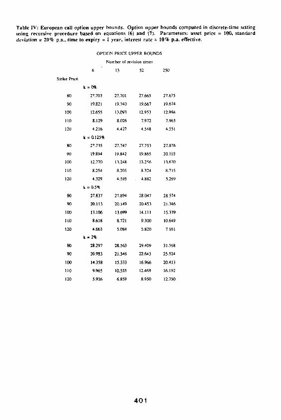
Tab le IV: E u r o p e a n call option u p p e r bounds. Opt ion uppe r bounds c o m p u t e d in d iscre te - t ime setting using recurs ive p r o c e d u r e based on equat ions (6) a nd (7). P a r a m e t e r s : asset pr ice = 100, s t a n d a r d deviat ion = 20% p.a., t ime to expi ry = 1 year , interest r a te = 10% p.a. effective.

Strike Price

OPTION PRICE UPPER BOUNDS

Number of revision times

13 52 250

k = 0 %

80 27.703 27.701 27.665 27.675

90 19.821 19.740 19.667 19.674

100 12.655 13.093 12.953 12.984

110 8.129 8.026 7.972 7.965

120 4.216 4.427 4.548 4.551

k = 0.125%

80 27.735 27.747 27.753 27.876

90 19.894 19.842 19.865 20.103

1(30 12.770 13.248 13.256 13.630

110 8.254 8.205 8.324 8.715

120 4.329 4.595 4.882 5.269

k = 0.5%

80 27.837 27.894 28.047 28.574

90 20.113 20.149 20.453 21.346

100 13.106 13.699 14.111 15.339

I10 8.618 8.721 9.3O0 10.649

120 4.663 5.084 5.820 7.161

k = 2 %

80 2K297 28.563 29.409 31.568

90 20.983 21.346 22.643 25.524

100 14.358 15.333 16.966 20.413

110 9.965 10.555 12.469 16.192

120 5.926 6.859 8.950 12.750

401

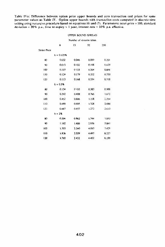
Tab le IVa: Di f fe rence be tween option price uppe r bounds and zero t r ansac t ion cost pr ices for same p a r a m e l e r va lues as T ab l e IV. Opt ion u p p e r bounds with t ransac t ion costs c o m p u t e d in discrete- t ime set l ing using recurs ive p r o c e d u r e based on equa t ions (6) and (7). P a r a m e t e r s : asset price = 100, s t anda rd devia t ion = 20% p.a., t ime to expi ry = 1 year , in teres t r a te = 10% p.a. effective.

Strike Price

LrPPER BOUND SPREAD

Number of revLsion lames

6 13 52 250

k = 0.1259~

80 0.032 0.046 0.089 0.201

90 0.073 O. 102 O. 198 0.429

100 0. I 15 0.155 0,30,t 0.646

110 0,124 0.179 0,352 0,750

120 0,113 0.168 0.334 0.718

k = 0.5%

80 0.134 0.193 0.383 0.900

90 0,292 0.408 0.786 1.672

100 0.452 0.606 1.158 2.354

110 0.489 0,695 1.328 2.684

120 0,4,:1.7 0,657 1,272 2,610

k = 2 %

80 0.594 0.862 1.744 3.893

90 1.162 1.606 2.976 5849

100 1.703 2.240 4.013 7.429

1 I0 1.836 2,529 4.497 8.227

120 1,710 2.432 4.402 8.199

4 0 2

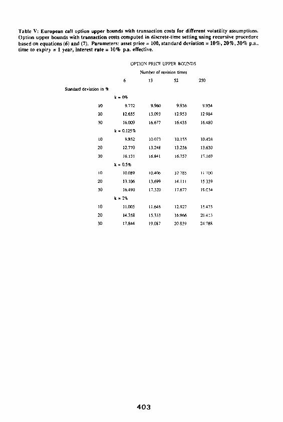
Table V: European call option upper bounds with transaction costs for different volatility assumptions. Option upper bounds with transaction costs computed in discrete-time setting using recursive procedure based on equations (6) and (7). Parameters: asset price = 100, s tandard deviation = 10%, 20%, 30% p.a., time to expiry = 1 year, interest rate = 10% p.a. effective.

Standaxd deviation in %

OF'TION PRICE UPPER BOUNDS

Number of revision times

6 13 52 250

k=0%

I0 9.772 9.960 9.936 9.954

20 12.655 13.093 12.953 12.984

30 16.009 16.677 16.435 16.480

k = 0.125%

10 9.852 10.073 10.155 10.424

20 12.770 13.248 13.256 13.630

30 16.131 16.841 16.757 17.169

k = 0.5%

I0 10.089 10.406 I0.785 I 1 7(30

20 13.106 13.699 14.111 15.339

30 16.490 17.320 17.677 19.034

k = 2%

10 11.005 11.646 12.927 15.475

20 14.358 15.333 16.966 20.413

30 17.844 19.087 20.839 24.788

4 0 3

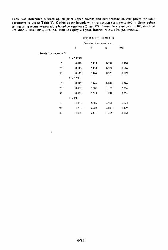
T a b l e Va: D i f f e r ence be tween op t ion p r i c e u p p e r b o u n d s a n d z e r o - t r a n s a c t i o n cost p r i ces for s ame p a r a m e t e r va lues as T a b l e V. O p t i o n u p p e r b o u n d s wi th t r a n s a c t i o n cos ts c o m p u t e d in d i sc re te - t ime se t t ing u s i n g r e c u r s i v e p r o c e d u r e b a s e d on e q u a t i o n s (6) a n d (7). P a r a m e t e r s : asset p r i ce = !00 , s t a n d a r d dev ia t ion = I 0 % , 2 0 % , 3 0 % p.a . , t ime to e x p i r y = 1 y e a r , in te res t r a t e = 1 0 % p .a . effective.

Sm,~dard devotion in %

UPPER BOUND SPREADS

Number of revtsion tames

6 13 52 250

k = 0.125%

10 0.079 0.113 0.218 0.470

20 0.115 0.155 0.304 0.646

30 0.122 0.164 0.323 0.689

k = 0.5%

10 0.317 0.446 0.849 1.746

20 0.452 0.606 1.158 2.354

30 0.481 0.643 1.242 2.554

k = 2 %

10 1.233 1.685 2.991 5.522

20 1.703 2.240 4.013 7.429

30 1.83,5 2.411 4.405 8.308

4 0 4

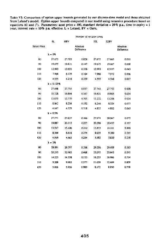
T a b l e VI: C o m p a r i s o n o f op t ion u p p e r b o u n d s g e n e r a t e d by o u r d i s c r e t e . t i m e mode l a n d those o b t a i n e d f r o m L e l a n d ' s mode l . O p t i o n u p p e r b o u n d s c o m p u t e d in o u r mode l u s ing r e c u r s i v e p r o c e d u r e based on e q u a t i o n s (6) a n d (7). P a r a m e t e r s : asset p r i ce = 100, s t a n d a r d dev ia t ion = 2 0 % p.a, , t i m e to e x p i r y = 1

year, interest rate = 10% p.a. effective. L = Leland, BV = Ours.

Strike Price

6L 6BV

k =0%

80 27.675 27.703

90 19.675 19.821

100 12.993 12.655

110 7.966 8.129

120 4.555 4.216

k = 0.125%

80 27.698 27.735

90 19.728 19.894

100 13.075 12.770

110 8.062 8.254

120 4.647 4.329

k = 0.5%

80 27.771 27.837

90 19.887 20.113

100 13.317 13.106

110 8.344 8.618

120 4.916 4.663

k = 2%

80 28.091 28.297

90 20.515 20.983

100 14.225 14.358

110 9.388 9.965

120 5.926 5.926

Number of ~v~ion ames

52L 52BV

Absolu~ Absolu~ Diff~cncc Difference

0.028 27.675 27.665 0.010

0.147 19.675 19.667 0.008

0.338 12.993 12.953 0.040

0.16,:1 7.966 7.972 0.006

0.339 4.555 4.548 0.007

0.037 27.745 27.753 0.008

0.167 19.831 19.865 0.034

0.305 13.232 13.256 0.024

0.192 8.246 8.324 0.077

0,318 4.822 4.882 0.060

0,066 27.974 28.047 0.073

0,227 20,296 20.453 O. 157

0.210 13.915 14.111 0,196

0.274 9.035 9.300 0.265

0.254 5.582 5.820 0.238

0.206 29.026 29.409 0.383

0.468 22.052 22.643 0.592

0.133 16.253 16.966 0.714

0.577 I 1.659 12.469 0.809

0.000 8.172 8.950 0.7'78

405

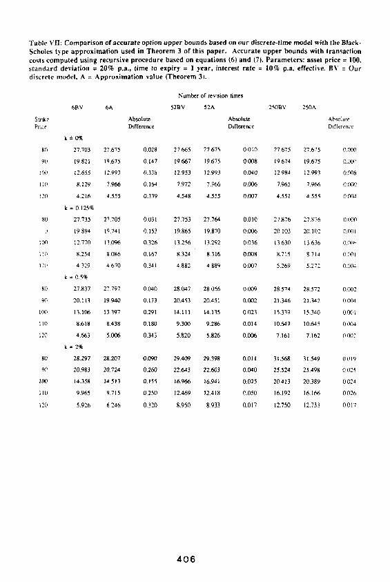
Table VII: Comparison of accurate option upper bounds based on our discrete-tlme model with the Black- Scholes type approximation used in Theorem 3 of this paper. Accurate upper bounds with transaction costs computed using recursive procedure based on equations (6) and (7). Parameters: asset price = 100, standard deviation = 20% p.a., time to expiry = 1 year, interest rate = 10% p.a. effective. BV = Our discrete model, A = Approximation value (Theorem 3).

Number of revision times

6BV 6A 52BV 52A 250BV 250A

Smke Absolute Absolute Absolute Price Difference Difference Difference

k~ -0%

80 27.703 27.675 0.028 27.665 27.675 0.010 27,675 27.675 0000

90 19.821 19.675 0.147 19.667 19.675 0.008 19,674 19.675 0.0()0

100 12.655 12.993 0.338 12.953 12.993 0.040 12984 12.993 0.008

110 8.129 7,966 0.164 7.972 7,966 O.0(k5 7,965 7.966 0000

120 4.216 4.555 0,339 4.548 4.555 0.007 4,551 4.555 0004

k = 0.125%

80 27.735 27.705 0.031 27.753 27,764 0.010 27.876 27.876 0.000

19.894 19.741 0.153 19.865 19.870 0.006 20,103 20.102 0001

i00 12.770 13.096 0.326 13.256 13.292 0.036 13.630 13.636 0 ~ e ,

110 8254 8.086 0.167 8.324 8.316 0.008 8.715 8714 0.001

120 4.329 4.670 0.341 4.882 4.889 0.007 5,269 5.272 O(X~

k = 0.5%

80 27.837 27.797 0.040 28.047 28,056 0.009 28,574 28.572 0002

90 20.113 19.940 0.173 20.453 20.451 0.002 21,346 21.342 O.(Y)4

I(X~ 13.106 13.397 0.291 14.111 14.135 0.023 15,339 15.340 0.00I

110 8,618 8.438 0.180 9.300 9.286 0.014 10,649 10.645 0004

120 4.663 5.006 0.343 5,820 5.826 0.006 7.161 7.162 0002

k = 2 %

80 28.297 28.207 0.090 29.409 29.398 0.011 31,568 31.549 0.019

90 20.983 20.724 0.260 22.643 22.603 0.040 25,524 25.498 0.025

100 14.358 14513 0.155 16.966 16.941 0.025 20,413 20,389 0.024

I10 9.965 9.715 0.250 12.469 12.418 0.050 16.192 16.166 0.026

120 5,926 6246 0.320 8.950 8,933 0.017 12,750 12.733 0017

4 0 6

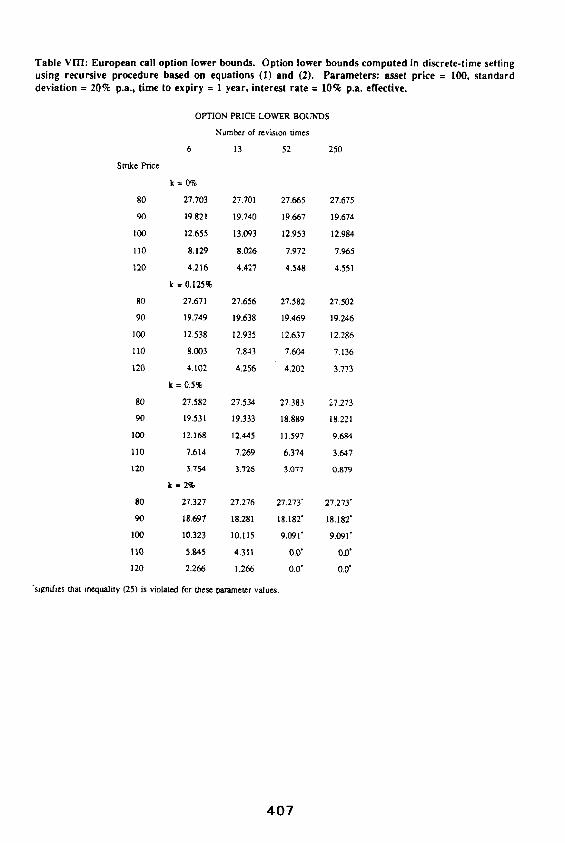
T a b l e VIII : E u r o p e a n call op t ion lower b o u n d s . O p t i o n lower b o u n d s c o m p u t e d in d i sc re t e - t ime set l ing us ing r e c u r s i v e p r o c e d u r e b a s e d on e q u a t i o n s ( I ) a n d (2). P a r a m e t e r s : asset p r i ce = I00 , s t a n d a r d dev ia t ion = 2 0 % p,a, , t ime to exp i ry = I y e a r , in te res t r a t e = 10% p,a, effect ive.

Strike Price

OPT/ON PRICE LOWER BOUNDS

Number of l'~vision times

13 52 250

k = 0%

80 27.703 27.701 27.665 27.675

90 19.821 19.740 19.667 19.674

1<30 12.655 13.093 12.953 12.984

110 8.129 8.026 7.972 7.965

120 4.216 4.427 4.548 4.551

k = 0.125%

80 27.671 27.656 27.582 27.502

90 19.749 19.638 19.469 19.246

100 12,538 12.935 12.637 12.286

110 8.003 7.843 7.604 7.136

120 4.102 4.256 4.202 3.773

k = 0.5%

80 27.582 27.534 27.383 27.273

90 19.531 19.333 18.889 18.221

100 12.168 12.445 11.597 9.684

110 7.614 7,269 6,374 3.647

120 3.75.4 3.726 3.077 0,879

k = 2 %

80 27.327 27,276 27.273" 27,273"

90 18.697 18.281 18.182" 18.182"

100 10.323 10.115 9.091" 9.091"

I 10 5.845 4.311 0.0" 0.0"

120 2.266 1.266 0.0" 0.0"

"signifies that inequality (25) is violawxl for these parameter values.

407

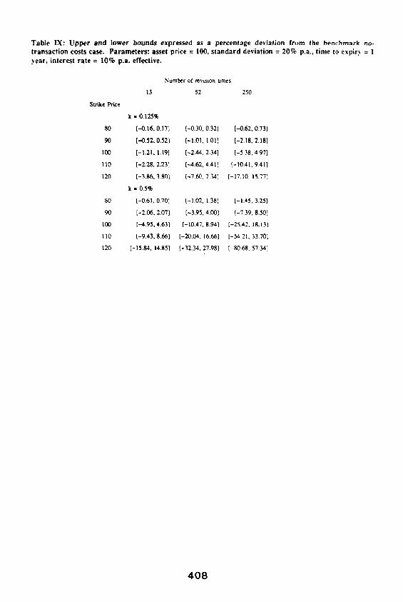
T a b l e IX: U p p e r a n d lower b o u n d s exp re s sed as a p e r c e n t a g e dev i a t i on from the b e n c h m a r k no- t r a n s a c t i o n cos t s case. P a r a m e t e r s : asse t p r i ce = 100, s t a n d a r d dev ia t ion = 2 0 % p.a. , t ime to expir.~ = 1 y e a r , in te res t r a t e = 1 0 % p .a . effect ive.

Number of revision umes

13 52 250

Strike Price

k = 0.125%

80 [-0.16, 0.17] [-0.30, 0.32] [-0.62, 0.73]

90 [-0.52, 0.52] [-1.01,101] [-2.18, 2.18]

1(30 [-1.21, 1 .191 [-2.44, 2.34] [-5.38, 4.97]

110 [-2.28, 2.23] [--4.62, 4.41] [-10.41, 9.41]

120 [-3.86, 3.80] [-7.60, 7.341 [-17.10, 15.77]

k - 0.5%

80 [-0.61, 0.70] [-1.02, 1.38] [-1.45, 3.25]

90 [-2.06, 2.07] [-3.95, 4.00] [-7.39, 8.50]

leo [--4.95, 4.63] [-10.47.8.94] [-25.42, 18.13]

110 [-9.43, 8.66] [-20.04. 16.66] [-54.21, 33.70]

120 [-15.84, 14.85] [-32.34, 27.981 [-80.68, 57.34]

4 0 8

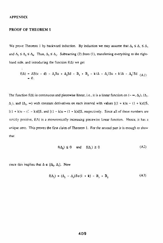
A P P E N D I X

P R O O F O F T H E O R E M 1

We prove Theorem 1 by backward induction. By induction we may assume that A4 < A~ < z~ 3

and A 5 _< A 2 _< A 4. Thus, A 2 _< Av Subtracting (2) from (1), transferring everything to the right-

hand side, and introducing the function f(A) we get

f(A) - AS(u - d) - A,Su + AzSd - B, + B z - klA - A, ISu + klA - A:[Sd (A1)

-- 0 .

The function f(A) is continuous and piecewise linear, i.e., it is a linear function, on ( - ,,,,, A,z), (A:,

A~), and (A~, ~o) with constant derivatives on each interval with values [(1 + k)u - (1 + k)d]S,

[(1 + k)u - (1 - k)d]S, and [(1 - k)u - (1 - k)d]S, respectively. Since all of these numbers are

strictly positive, f(A) is a monotonically increasing piecewise linear function. Hence, it has a

unique zero. This proves the first claim of Theorem 1. For the second part it is enough to show

that

f(A 2) < 0 and f(A,) > 0 (A2)

since this implies that A ~ [A 2, At]. Now

f ( ~ ) - (a~ - A , ) S u ( 1 + k) - B, + B 2 (A3)

409

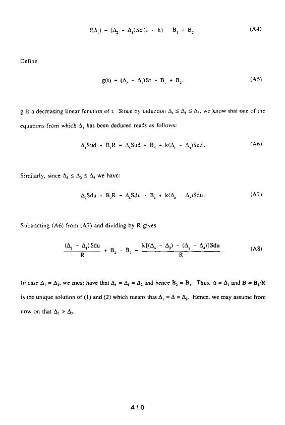
f(Aa) - (A 2 - A1)Sd( I - k) - B t + B: . (A4)

De f ine

g(t) - (A 2 - AI)St - B z + B: . (A5)

g is a d e c r e a s i n g l inear func t ion o f t. S ince by induc t ion A4 -< A~ _< '~3, w e k n o w that one o f the

e q u a t i o n s f rom wh ich A~ has been d e d u c e d reads as fo l lows:

A1Sud + BIR - A4Sud + B 4 + k(A I - A , )Sud . (A6)

Simi lar ly , s ince A~ < A 2 _< A, we have:

A~Sdu + BzR - A4Sdu + B 4 + k(A, - A2)Sdu. (A7)

Sub t rac t ing (A6) f rom (A7) and d iv id ing by R g i ve s

( A 2 - A , ) S d u k [ ( A , - A2) - (A , - A , , ) ]Sdu + B= - Bs - (A8)

R R

In case A t = A2, we m u s t h a v e that A, = A t = A: and h e n c e B: = B v T h u s , A = A~ and B = Bt /R

is the u n i q u e so lu t ion o f (1) and (2) w h i c h m e a n s that A~ = A = A 2. Hence , w e m a y a s s u m e f rom

n o w on that A s > A 2.

4 1 0

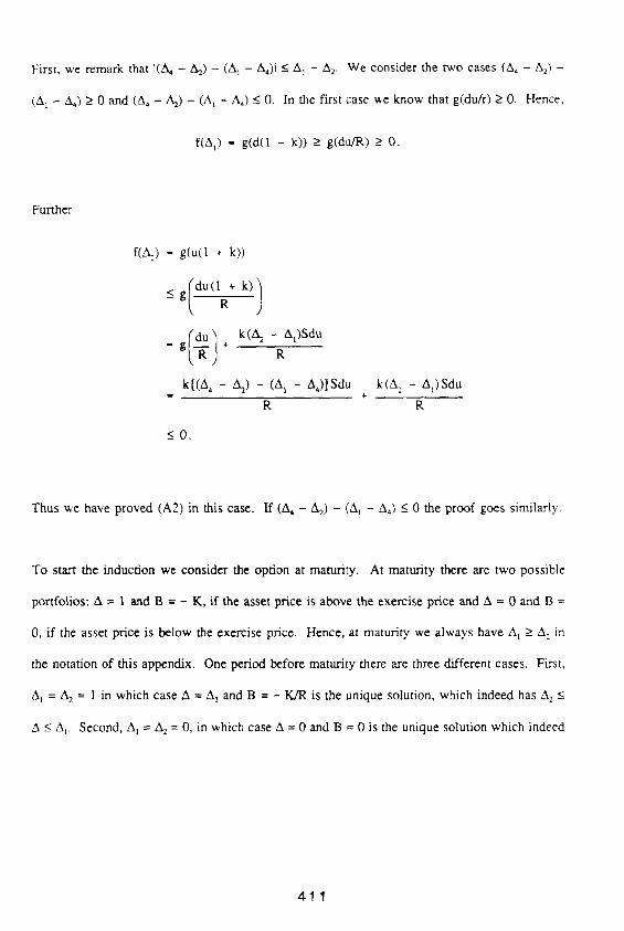
First , we remark that 1(,5, - ~ ) - (A~ - A4)I _< A~ - A 2. We cons ider the two cases (A, - A 2) -

(A1 - A4) >- 0 and (A,~ - A z) - (A~ - A,,) _< 0. In the first case we know that g(du/r) > 0. Hence ,

f(A,) - g(d(1 - k)) -> g(du/R) _> 0.

Fur ther

f ( @ - g(u(1 + k))

< g / d u ( 1 ÷ R" k))

( _ ~ ) k ( , - A,)Sdu

= g + R

k[ (~° - A~) - (A, - A , ) lSdu

R

-<0 .

kfA: - A~)Sdu +

R

T h u s we have p roved (A2) in this case. If (A4 - A2) - (A~ - A4) < 0 the p roo f goes s imilar ly .

To start the induc t ion we cons ide r the opt ion at matur i ty . At matur i ty there are two poss ib le

por t fo l ios : A = 1 and B = - K, if the asset pr ice is a b o v e the exerc i se pr ice and A = 0 and B =

0, if the asset pr ice is be low the exerc i se price. Hence , at matur i ty we a lways have A~ _> A 2 in

the no ta t ion o f this appendix . One per iod before matur i ty there are three d i f fe rent cases. First,

A~ = A 2 = 1 in which case A = A~ and B = - K/R is the unique solut ion, wh ich indeed has ,5 2 <

A .<_ A~. Second , A] = A~ = 0, in which case A = 0 and B = 0 is the unique solut ion which indeed

41"T

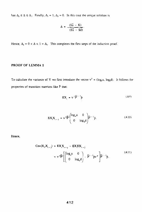
h a s A 2 - < A < - A 1. Finally, A t = 1, A 2 = 0 . In this case the unique solution is

A - (S~ - K)

( S t - Sd)

Hence , A 2 = 0 < ,5 < 1 = A t. This comple t e s the first steps o f the induct ion proof.

P R O O F O F L E M M A 1

To calculate the var iance o f Y we first in t roduce the vec tor v r = (log, u, log,d). It fo l lows for

proper t ies o f t ransi t ion mat r ices like f ' that:

EX, - v r P i - ~ (A9~

°

° = V "r~J cU

EXiX' "J log,,d P" (AIO)

Hence ,

C o v ( X e X i . j) - EXiX i . j - EXlEX i . j

In p.

(A11)

412

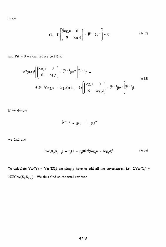
Since

r o,.u ° (A12)

and PA = 0 we can reduce ( A l l ) to

ICo: o 1_ vT(OA) j u log,d P "

0)_ log d

~ L - I ~ V T

(AI3)

p

If we denote

~ i - I f ) . ( p , , 1 - p i ) T

we find that

Cov(X~,X~.j) - p~(1 - p)0J2J(log u - log d) 2 (A14)

To calculate Vat(Y) = Var(~X~) we simply have to add all the covariances, i.e., ZVar(X,) +

2EZCov(X,,X i + j). We thus find as the total variance

4 1 3

( log u - l o g , d ) : p,(1 - p ) (20) j - 1 - L , - t .~

I~ IE ] ( l o g , u - l o g , d ) : pi(1 - p,) 2 ,1 - (20) . . . . I _

, 1 7 ~

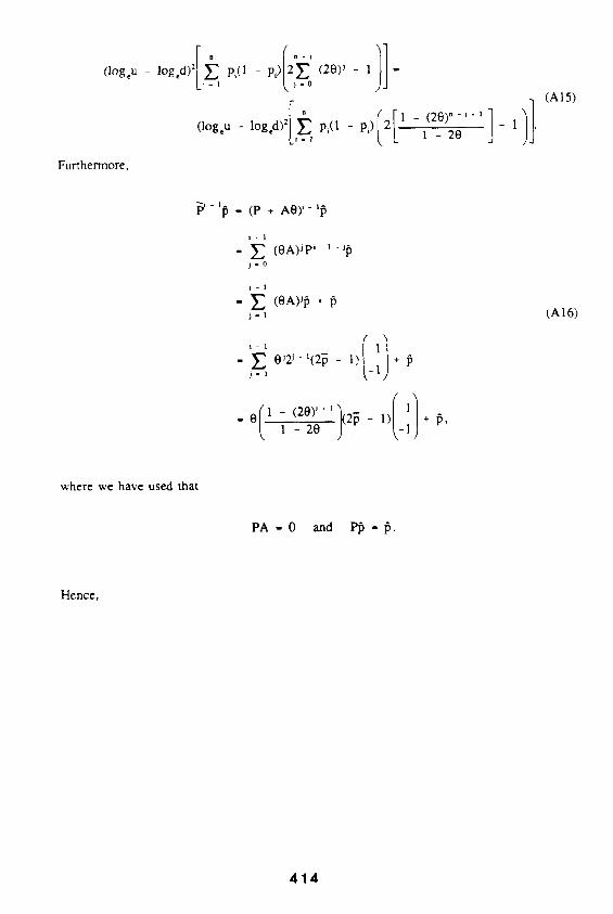
F u r t h e r m o r e ,

'/1. (A15)

(P + A O ) ' - i ~

i - 1

( 0 A ) J P ' - ' - it3 j ° 0

i - !

j o l

0~2 j " ~(2~ - I ) * ) o l

't ¸ (,

(A16)

w h e r e w e h a v e u s e d that

P A - 0 and PIb - ~ .

H e n c e ,

4 1 4

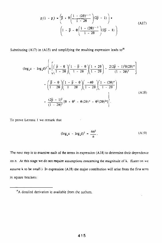
P,(l - P,) -

(A171

Substituting (A17) in (A15) and simplifying the resulting expression leads to”

(A181

To prove Lemma 1 we remark that

(logcu - log,d)* - y. (AI91

The next step is to examine each of the terms in expression (A 18) to determine their dependence

on n. At this stage we do not require assumptions concerning the magnitude of k. (Later on we

assume k to be small.) In expression (A18) the major contribution will arise from the first term

in square brackets:

“A detailed derivation is available from the authors.

415

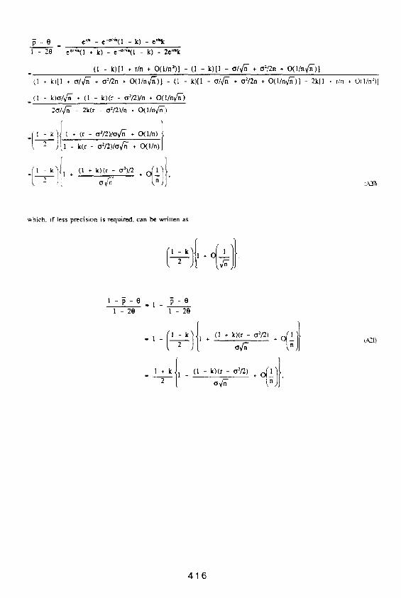
g - o 1 - 2 0

e '~' - ¢ ~ r ~ ( l - k ) - e ' t ' k

e " ~ ' ( 1 + k ) - e - " ' ~ ' ( l - k) - 2e '~ 'k

( l - k ) [ 1 * r/n ÷ O ( l / n * ) ] - (1 - k ) [ 1 - o / ~ h - , o = / 2 n ÷ O ( 1 / n f ~ ) l

t l + k ) [1 , o . / f n - + ~2 /2n , O ( 1 / n v " n " ) l - (1 - k ) [ l - er/,/-fi- + a :P2n , O ( 1 / n v ~ - ) ] - 2 k [ l ÷ r/n ,- O ( I / n : ) ]

. ( I - k)(Ylv/~ - + ( t - k ) ( r - ( r2/2) In + O ( I / n V ~ - )

2 o / ¢ ~ - - 2 k ( r - o2 /2 ) /n + O ( I / n ¢ ~ - )

1 - k ( r - c2/2) l~ fn ÷ O ( 1 / n )

w h i c h , i f l e s s p r e c i s i o n is r e q u i r e d , c a n b e w r i t t e n a s

÷

I - ~ - O 1 - 2 0

l _~ -e 1 - 2 e

, ~ +

(A21)

4 1 6

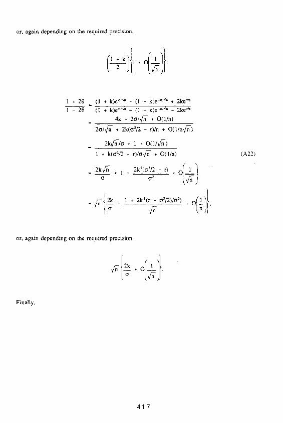
or, again depending on the required precision,

1 + 2 0

1 - 20

(1 + k)e °l~* - (1 - k)e -°j~n + 2ke '~

(1 + k)e °j~° - (1 - k)e -°1~* - 2ke '~

4k + 2cs/V~- + O(1/n)

2g/ fn ' - + 2k(~2/2 - r)/n + O(l/nv/-n -)

2kv/-n-/o + 1 + 0(1/7~-)

1 + k(~2/2 - r)/(wt-n + O(1/n)

2k¢~- 1 2k2(cz/2 - r) a + - a 2 + 0 / ~ n n / 1

(A22)

or, again depending on the required precision,

+ O 1

Finally,

4 1 7

o ,11~2o_,1 1 - 2 0 4 1 - 2 0

1 1 + 2 0 2 0

1 - 2 0 1 - 2 0 1 - 2 0

O 1

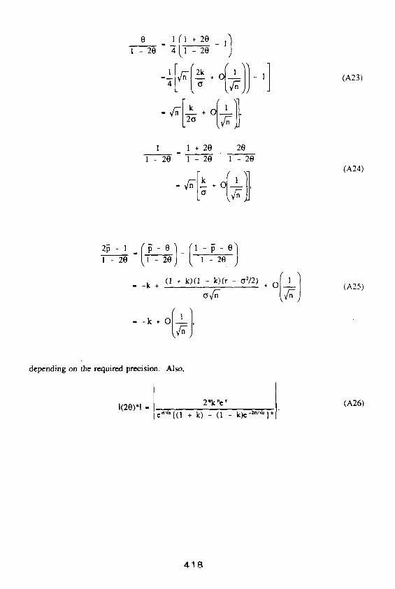
(A23)

(A24)

1 - 2 0

- - k + ( l + k)(1 - k)(r - o212)

, 1 (A25)

depending on the required precision. Also,

!

2*k *c ' I 1(20) '1- e~v.{( 1 + k) - (1 - k)e-~/~*} .1"

(A26)

4 1 8

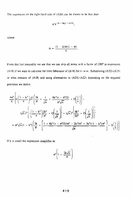
The expression on the right-hand side of (A26) can be shown to be less than

e re-[e - I05.(I * e ) l ~ a

where

( 1 - k ) c r ( 1 - ~) a -

From this last inequality we see that we can skip all terms with a factor of (20)* in expression

(A18) if we want to calculate the limit behaviour of (A18) for n ----> ,~. Substituting (A20)-(A25)

in what remains of (A18) and using alternatives in (A20)-(A22) depending on the required

precision we derive

2 { n i l - k2"~-n I2k + 1 6k=(r - 02/2) + O(1"~ 4~ ~, 4 ) ~,o "~--n + a2v~- t n ] j ÷

( c--''zl ~ 1 - k2"~2k2 ~-~-n 1 } f 43~ko~ ~'~'n 1}} q n ) [ - I.-----~--- ~..-~- + + ( vr~ )2 + 1

- o ' v ~ - ( l - kZ)[-~-+ [1 + 6k2(r-c2,2)/o 2 -2k2/o: + 3 k ' , ( l ~ - k~,o 2

If k is small the expression simplifies to

4 1 9

This completes the proof of Lemma 1.

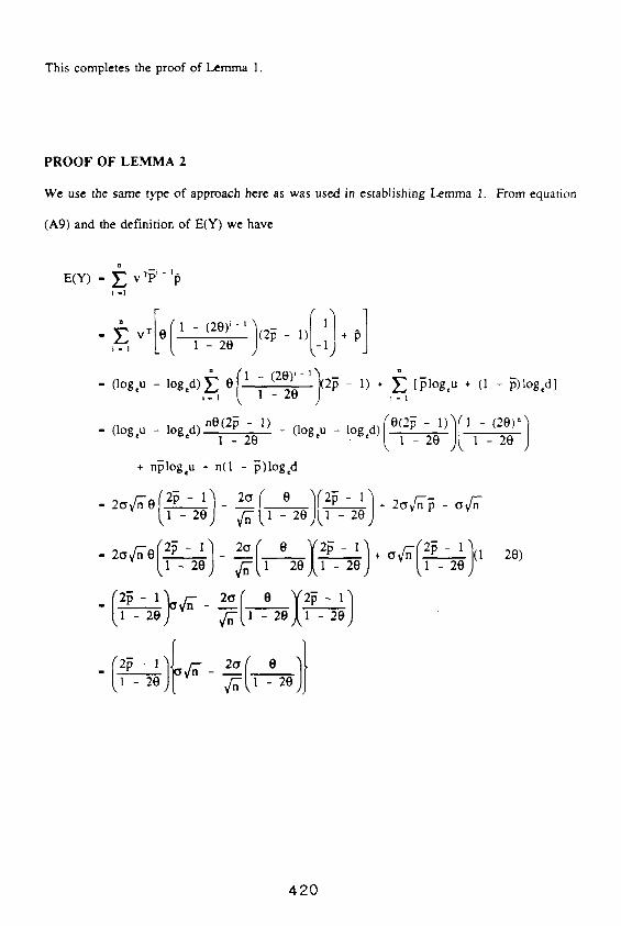
P R O O F O F L E M M A 2

We use the same type of approach here as was used in establishing Lemma 1. From equation

(A9) and the definition of E(Y) we have

E(Y) - L v ' r # i - l ~ i - |

I I ' l l - v T 0 1 - ( 2 0 7 - ' ( 2 ~ - 1) + , . , i - ~ -1

- (log u - log d ) ~ l e .1 - (2e) ' -1 7 - ' ~ 2p - 1) + [ p l o g u + (1 - ~ ) l o g d ] - i - 1

1 - 2 8 - 1 - 2 0 )

+ n~log u + n(1 - ~ ) log ,d

c,-~oj ~-t,-~ojt,-~oj < ' ~ I ~ ) ' - ~ . r ~ - ' b , r ; - ~ r o ¥ ~ _ , ]

t.1 - 2 0 7 vn ~ t i - 20Jr.1 - 201

, / ; t 1 - 2 e ) j

420

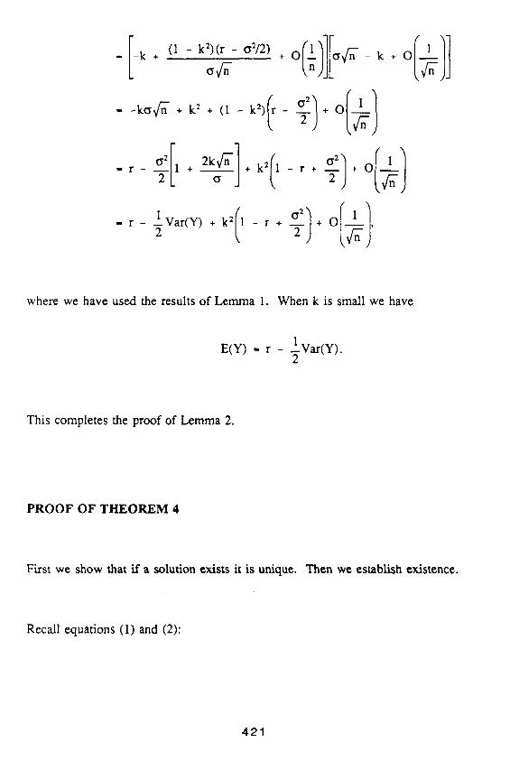
E- ( I]E o o/ l] - k (1 - k2)(r - o'2/2) + 0 ~ - k +

-~[1 2k~/'n'-] k211 -~1 I~n-nl - r - + + - r + + O 1

- r - 1 V a t ( Y ) + kZll - r + -~1+ O(.~n-n;,

where we have used the results of Lemma 1. When k is small we have

1 E(Y) .. r - _" Vat(Y).

2

This completes the proof of Lemma 2.

P R O O F O F T H E O R E M 4

First we show that if a solution exists it is unique. Then we establish existence.

Recall equations (1) and (2):

421

A S u + B R - AISu + B 1 + k lA - A l l S u ( I )

A S d + B R - A2Sd ÷ B 2 + k l A - A.21Sd. ( '2)

S u b t r a c t i n g (2) f r o m (1) a n d t r a n s f e r r i n g e v e r y t h i n g to the r i g h t - h a n d s ide ,

f (A) - A S ( u - d) - A t S u + A2Sd - B 1 + B 2 - k l A - A l l S u + k l A - A.21Sd

- 0 .

T h e r e are t w o p o s s i b l e c a s e s : A t < ,52 a n d A 1 > A:.

W h e n A t _< A 2, f (A) is a l i n e a r f u n c t i o n on (---,=,,At), (A1,,5,2), a n d (A:,oo), w i t h c o n s t a n t d e r i v a t i v e s

o n e a c h i n t e r v a l w i t h v a l u e s

(1 + k ) S ( u - d ) , [(1 - k ) u - (1 + k ) d ] S , a n d 1 - k ) ( u - d ) S ,

r e s p e c t i v e l y . I f ( l - k )u > (1 + k)d , all o f t h e s e d e r i v a t i v e s a re p o s i t i v e , a n d f fA) is an i n c r e a s i n g

f u n c t i o n .

W h e n A t > A2, f (A) is a l i n e a r f u n c t i o n on (--00,A2), (A2,AI), a n d (At,*"), w i t h c o n s t a n t d e r i v a t i v e s

on e a c h i n t e r v a l w i t h v a l u e s

(1 + k ) S ( u - d ) , [(I + k ) u - (1 - k ) d ] S , a n d (1 - k ) ( u - d ) S ,

4 2 2

respectively. All of these derivatives are positive, and therefore, f(A) is an increasing function.

Thus, f(A) is a monotonically increasing function. Hence, if f(A) has a zero, it has a unique zero,

i.e., the system has a unique solution.

We now prove that a solution to equations (1) and (2) always exists.

Select Ao~ such that

031 - B2) ÷ (1 + k)S(Alu - A~d) Aol < and Ao, _< min{A,,A=}.

(1 ÷ k)S(u - d)

Select A0z such that

031 - B:) ~- (1 - k)S(Alu - A2d) A°2 > (1 - k)S(u - d) and A0~ _> max {A z, A2}.

It is easy to show that f(Ao~)< 0 and f(Ao2) > 0. Since f(A) is a continuous function, there exists

a A, (Ao~ < A < Ao2), such that f(A) = 0. This completes the proof of Theorem 4.

4 2 3

424