AD A124 017 STUDIES OF HEAT TRANSFER IN COMPLEX INTERNAL FLOWS(U) 1/2MINNESOTA UNIV MINNEAPOLIS DEPT Of MECHANICALENGINEERING E M SPARROW JAN 83 NOO014-79-C-0621

LIFEED F/G 13/1 NL

mohhhhEohhohEEmIIEEE-IIIIIIEmhhllllllhlll*EEEEEEEEEE///lllllllllllllEIIIIIIIIIIIIhlIIIIIIIIIIIIImlllllllllllIIo

1.02.2

uflu.~lu

-~ ,,

III.25 11 1. 4 11I1.6

miCRocoPY RESOLUTION TEST CHART

NAINLBREUO'TNDRS16-

bo

I STUDIES OF HEUT TRANSFER IN COFLE INTERNAL FLOWS

E. M. Sparrow

I

Third Suumary Report

Contract N00014-79-C-0621

Office of Naval Research

I

I January, 1983

I

I Department of Mechanical Engineering

S,-,University of Minnesota DT ICS..Minneapolis, Minnesota 55455 ELECTE

C-Z)S FES I D

SDISTRIBUTION STATEMENT A 01 07Approved fotpublic resel 8.1 Distuibution JUlimitd8 1. 8

LCU ITY CLASSIFICATION OF THIS PAGE (When D ei En eed) R

REPORT DOCUMENTATION PAGE EFORE COMPLETING R

I REPORT NUMBER G VT ACCESSION NO. 3. NCIPIENT'S CATALOG NUMBER

NOOO14-79-C-O621-19A. jAA,- 4/, 74 TITLE (and S,.bli(1) 5. TYPE OF NREPORT A PERIOD COVERED

STUDIES OF HEAT TRANSFER IN COMPLEX Summaty ReportDec.15,1981 to Dec.15,1982INTERNAL FLOWS G. PERFORMING ORG. REPORT NUMBER

7 AUTHOR(e) 6. CONTRACT OR GRANT NUMBER(.)

E. M. Sparrow N00014-79-C-0621

PERFORMING ORGANIZATION NAME AND ADDRESS I0. PROGRAM ELEMENT. PROJECT. TASK

AREA 6 WORK UNIT NUMBERS

Department of Mechanical Engineering

University of Minnesota, Minneapolis, MN. 55455 Work Unit NR097-437

II . CONTROLLING OFFICE NAME AND ADDRESS 12. REPORT DATE

Office of Naval Research January, 1983800 North Quincy Street I3 NUMBER OF PAGES

Arlington, Virginia 22217 10214 MONITORING AGENCY NAME G AODRESS(II dillerent from Controlling Office) IS. SECURITY CLASS. (of thls report)

Unclassified

ISe. DECL ASSIFICATION/DOWNGRADINGSCHEDULE

lb DISTRIBUTION STATEMENT (of tli Report)

Approved for public release; distribution unlimited

17 DISTRIBUTION STATEMENT (of the obltrect entered In Block 20, II dilerent from Report)

I4 SUPPLEMENTARY NOTES

19 KEY WORDS (Continue on reveres aide It necesmy end IdentIty by block number)

heat exchangers, flow maldistribution, heat transfer coefficient, pressuredrop, tube bank, plenum chamber, swirl

7/

MO. STRACT (Conlinue an reveree side It necesaey and Identify by block number)

Experiments have been performed to determine the heat transfer andpressure drop response of heat exchange devices subject to highly complexfluid flows. Three research problems were undertaken and completed, each

dealing with a different aspect of heat exchanger performance. In onecase, per-tube transfer coefficients were measured in a tube bank in thepresence of an abrupt upstream enlargement of the flow cross section.

DD 1',AR, 1473 EOTION OF 1 NOV 65 IS OBSOLETE UnclassifiedS.'N 0102-LF-04.6601

SECURITY CLASSIFICATION OF THIS PAGE (Men Date Enter"O)T

SECURITY CLASSIFICATION OF THIS PAGE (When Da Enterd)

-it iEnhancement of the heat transfer was found to occur as a result of theV

flow disturbances caused by the enlargement. In the second researchproblem, the effect on heat transfer of the competition between tubeswhich draw air from a common plenum was investigated. This competitionresulted in a skewing of the flow entering the tubes. Significanteffects of the skewing occurred when the tubes were relatively closetogether (pitch 'v 1.5 tube diameters), but for larger spacings theheat transfer coefficients were virtually identical to those for asingle tube.> " I (,

>In the last of the problems, the effects of flow maldistribution

caused by partial blockage of the inlet of a flat rectangular duct wereinvestigated. Large spanwise nonuniformities of the local heat transfercoefficient were induced by the maldistributed flow. The spanwise-average heat transfer coefficients in the downstream portion of the ductwere found to be enhanced due to the flow maldistribution, whereas atmore upstream locations a reduction of the coefficients occurred.

Accession ForNTIS GRA&I

DTIC TAB 0Unannounced 0Justification

Distribut ion/

Availability CodesAvail and/or -----

Dist Special

UnclassifiedSECURITY CLASSIFICATION OF THIS PAGE(lhm O9*0 Enter*4

INTRODUCTION TO THE REPORT

The heat exchange devices that are employed in power producing systems are

subject to highly complex fluid flows whose effect on performance is generally

unknown. In this regard, information available in the literature is not readily

applicable since, for the most part, it is based on studies of relatively simple

flows and of elementary geometrical configurations. Even when more complex

devices are studied, only overall data are collected, so that the causes of

observed effects have not been identified.

As an example of the encountered flow complexities, attention may be called

to the possible maldistribution of the flow delivered to the heat exchanger

inlet, a case in point being Navy shipboard heat recovery which utilizes hot

gases exhausted from gas turbines. The maldistribution may result from changes

in cross section (e.g., sudden enlargement), partial blockages due to valves

and other control devices, changes in direction due to bends and elbows, and

branching and merging of flow passages. Frequently, more than one of these

features occur in a single system. The maldistribution may be accompanied by flow

separation, recirculation, and swirl.

Departures from ideal inlet conditions may also occur when parallel flow

passages draw fluid from a common plenum and, in the process, compete with each

other. Skewing of the flow entering the respective passages will occur unless

the plenum is very large, and the skewing will be accentuated if there is any

imbalance among the flow rates in the individual passages.

It is interesting to note that the turbulence and mixing inherent in

highly complex flows might serve to enhance the overall heat transfer performance.

Such an outcome, if true, would be an unexpected dividend, but it would have to

be weighed along with the inevitable pressure drop penalty. Whether or not there

- ----

2

is a net enhancement or degradation of heat exchanger performance depends on

the conditions under which the system is to be operated. For example, in certain

instances, the pressure drop in the heat exchanger may not be a critical factor,

as would occur if there were relatively large pressure drops in other portions

of the piping circuit. On the other hand, if significant reductions in flow

rate are required in response to the larger maldistribution-related pressure drop,

then the performance of the heat exchanger may be degraded.

The foregoing discussion serves to motivate and focus the research that is

described in this report. The underlying thrust of the work is to deal with

problems related to the realities of actual heat exchange devices, where the

fluid flow configuration is sufficiently complex that available information is

inapplicable. The report describes three research problems on which work was

performed and completed during the current reporting period. These problems are

1. Heat transfer in a tube bank in the presence of upstream

cross-sectional enlargement

2. In-tube heat transfer for skewed inlet flow caused by competition

among tubes fed by the same plenum

3. Maldistributed-inlet-flow effects on turbulent heat transfer

and pressure drop in a flat rectangular duct

Journal articles have been prepared for each of these problems. The manuscripts

for these articles have been brought together here to form the report for the

year's research activities.

:1

HEAT TRANSFER IN A TUBE BANK IN THE PRESENCE

OF UPSTREAM CROSS-SECTIONAL ENLARGEMENT

ABSTRACT

Per-tube heat transfer coefficients were determined in a tube bank in the

presence of an abrupt upstream enlargement of the flow cross section. The enlarge-

ment occurred either at the inlet face of the tube bank or at the upstream end of

a duct which delivered the flow to the inlet. Three different magnitudes of en-

largement were investigated along with three lengths of the delivery duct. Axial

pressure distributions were measured both in the tube bank and in the delivery duct,

and flow visualization was performed to observe the fluid motions in the tube bank.

It was found that the enlargement can give rise to appreciable increases in the

tube-bank heat transfer coefficients compared with those for the no-enlargement

case. The enlargement also causes an additional pressure drop which depends on the

magnitude of the enlargement and, to a lesser extent, on the distance between the

enlargement and the tube bank.

NOMENCLATURE

Amin minimum free flow area between tubes

D tube diameter

diffusion coefficient

f friction factor

K per-tube mass transfer coefficient

m rate of mass transfer per unit area

Nu0.7 Nusselt number corresponding to Pr = 0.7

Pr Prandtl number

ii

p pressure

Patm ambient pressure

APuncr enlargement-related incremental pressure drop

Re Reynolds number pVD/hi

S side of square duct

Sc Schmidt number

Sh per-tube Sherwood number, KD/X

SL longitudinal pitch

ST transverse pitch

V maximum velocity, 4/pAmin

w mass flow rate

X axial coordinate

I viscosity

V kinematic viscosity

p air density

Pnw naphthalene vapor density at tube surface

Pnb naphthalene vapor density in bulk flow

------------------ :J"-

I

INTRODUCTION

In tube-bank crosaflow heat exchangers, the crossflow fluid may be delivered

to the bank via a duct whose cross section differs from the inlet-face cross section

of the bank. Frequently, the area of the inlet face is substantially larger than

the cross-sectional area of the duct, necessitating an enlargement either at or

upstream of the inlet. Cross-sectional enlargements generally give rise to separa-

tion and accompanying flow disturbances, except for gradually tapered enlargements

which are rarely encountered in heat exchanger practice because of space limitations.

Most commonly, the enlargement is accomplished either abruptly or by means of a

rapid taper. Depending on the distance upstream of the tube bank inlet at which

the enlargement occurs, the highly disturbed flow which it spawns may have a sig-

nificant effect on the heat transfer and pressure drop characteristics of the bank.

The objective of the experiments to be reported here is to determine the heat

transfer and pressure drop response of a tube bank to an abrupt enlargement of the

flow cross section which occurs either upstream of or at the bank inlet. Measure-

ments were made of the per-tube heat transfer coefficient at each tube in each

successive row, starting at the first row and proceeding downstream until fully de-

veloped conditions were encountered. Pressure drops were also measured on a row-by-

row basis. To supplement the heat transfer and pressure drop data, flow visualiza-

tions were performed within the tube bank to observe the paths followed by the

disturbances generated by the upstream cross-sectional enlargement.

The experiments encompassed a total of nine different ducting arrangements.

These included three lengths of the duct which delivers the flow to the tube bank

inlet face and three enlargements of the flow cross section. The enlargement occurs

at the upstream end of the delivery duct, so that the chosen ducting arrangements

position the enlargement at various distances from the tube bank inlet face. To

provide a basis for assessing the effect of the enlargement, the aforementioned ex-

periments included the case of no enlargement. For each of the ducting arrangements,

-------

2

measurements were made for two Reynolds numbers which spanned an order of magnitude.

The heat transfer results will be presented in a format designed to provide

an immediate indication of the effect of the enlargement. At each tube in the

bank, the heat transfer coefficient in the presence of enlargement is ratioed with

that for the no-enlargement case, with all other geometrical and flow parameters

being held fixed. If this ratio exceeds one, then the enlargement is enhancing,

while values of the ratio below one indicate degradation. The ratios which pertain

to the respective tubes are inscribed on a plan-view layout of the bank, thereby

facilitating the identification of which portion of the bank is affected by the

enlargement.

The measured pressure distributions yielded fully developed friction factors in

the tube bank and incremental pressure losses associated with the presence of the

enlargement. The flow visualization work was carried out using the oil-lampblack

technique, and zepestaiLative photographs of the flow traces are included in the

paper.

The flow nonuniformity induced by an abrupt enlargement situated either at or

upstream of the inlet face of a tube bank can be regarded as a maldistribution. In

the heat exchanger literature, there is a keen awareness of the potential importance

of maldistributed inlet flows on the performance of the exchanger, as witnessed

Dy several papers in a just-published symposium volume {}. However, a careful

literature search did not reveal any published quantitative information on the

effect of upstream cross-sectional enlargement on the heat transfer and pressure

drop in a crossflow tube bank.

3

THE EXPERIMENTS

As noted earlier, the work included three types of experiments--heat transfer,

pressure drop, and flow visualization. Both from the standpoint of higher accuracy

and of experimental simplicity, mass transfer experiments offer several advantages

compared with direct heat transfer experiments. In the present study, the naph-

thalene sublimation technique was employed to determine mass transfer coefficients

which can be transformed to heat transfer coefficients by means of the analogy be-

tween the two processes.

The description of the experimental apparatus is facilitated by reference to

Fig. 1. The diagram at the upper part of the figure shows the inlet face of the

tube bank. As seen there, the cross section of the duct in which the tube bank is

housed is a square of side S. The lower part of the figure is a plan view looking

downward into the apparatus (as if the upper wall were removed). This diagram

shows a portion of the tube bank and the entirety of the delivery duct which con-

veys fluid to the inlet face of the bank. The delivery duct is, in effect, an up-

strea. !xtension of the duct which houses the tube bank. It is straight and of

square cross section with side S.

The different lengths of the delivery duct employed during the experiments can

be identified in Fig. 1. For the longest duct, the length is about 4.5S, while the

length of the intermediate duct is about 2.5S. The shortest duct is of zero length.

The delivery duct--tube bank system was operated in the suction mode. Air

was drawn from the laboratory room into the upstream end of the delivery duct or,

for the delivery duct of zero length, directly into the inlet face of the tube bank.

The air passed through the delivery duct and the tube bank, through a square-to-

circular transition section, and then through an air-handling system consisting of

flowmeters (calibrated rotameters), control valves, and blowers. The blowers were

situated outside the laboratory so that their discharge, which was heated by com-

pression and also contained naphthalene vapor, would not be recycled through the

4

experimental apparatus.

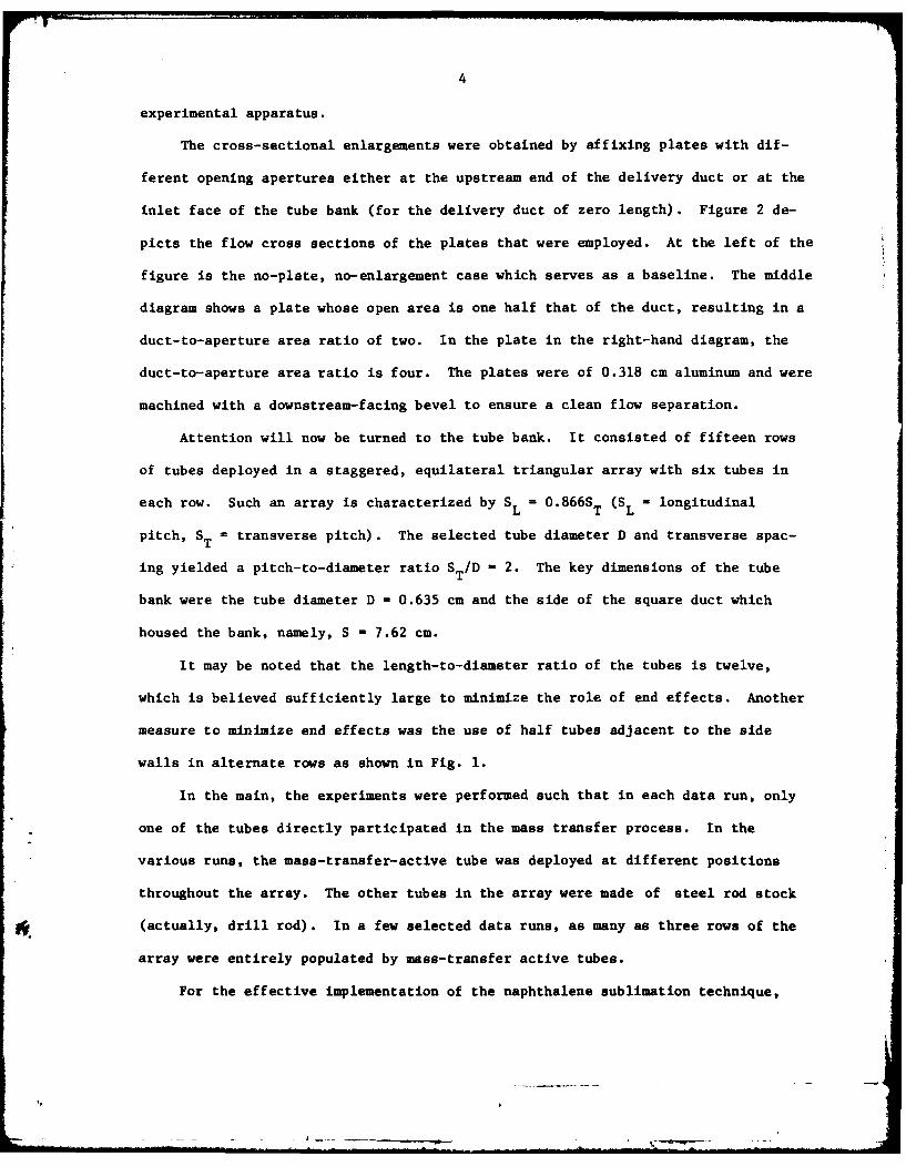
The cross-sectional enlargements were obtained by affixing plates with dif-

ferent opening apertures either at the upstream end of the delivery duct or at the

inlet face of the tube bank (for the delivery duct of zero length). Figure 2 de-

picts the flow cross sections of the plates that were employed. At the left of the

figure is the no-plate, no-enlargement case which serves as a baseline. The middle

diagram shows a plate whose open area is one half that of the duct, resulting in a

duct-to-aperture area ratio of two. In the plate in the right-hand diagram, the

duct-to-aperture area ratio is four. The plates were of 0.318 cm aluminum and were

machined with a downstream-facing bevel to ensure a clean flow separation.

Attention will now be turned to the tube bank. It consisted of fifteen rows

of tubes deployed in a staggered, equilateral triangular array with six tubes in

each row. Such an array is characterized by SL = 0.86 6ST (SL = longitudinal

pitch, ST = transverse pitch). The selected tube diameter D and transverse spac-

ing yielded a pitch-to-diameter ratio S T/D - 2. The key dimensions of the tube

bank were the tube diameter D = 0.635 cm and the side of the square duct which

housed the bank, namely, S - 7.62 cm.

It may be noted that the length-to-diameter ratio of the tubes is twelve,

which is believed sufficiently large to minimize the role of end effects. Another

measure to minimize end effects was the use of half tubes adjacent to the side

walls in alternate rows as shown in Fig. 1.

In the main, the experiments were performed such that in each data run, only

one of the tubes directly participated in the mass transfer process. In the

various runs, the mass-transfer-active tube was deployed at different positions

throughout the array. The other tubes in the array were made of steel rod stock

(actually, drill rod). In a few selected data runs, as many as three rows of the

array were entirely populated by mass-transfer active tubes.

For the effective implementation of the naphthalene sublimation technique,

.. .. .... .... . I .. .. .. . . ...

5

it is necessary that there be rapid access to the test section for the installation

or remvoal of the mass-transfer-active tubes. This is because sublimation, while

much diminished, continues to occu.r even when there is no airflow in the test sec-

tion. The required access was achieved by making the upper wall of the test section

removable, with quick-acting clamps being used to lock the wall in place during

the data runs.

The mass-transfer-active tubes consisted of a naphthalene coating over a

cylindrical metal substrate. The surface of the substrate had been roughened by a

screw-threading operation to provide better adhesion of the naphthalene. With re-

gard to the coating process, it consisted of two distinct stages. In the first

stage, the substrate was dipped repeatedly into a pool of molten naphthalene, which

produced a somewhat rough, overly thick coating. The desired final dimensions and

surface finish were obtained by machining the napthalene surface on a lathe. The

finished dimensions of the naphthalene-coated tubes were identical to those of the

steel rods which comprised the other tubes of the array.

Each mass transfer data run consisted of two distinct parts: the equilibra-

tion period and the data run proper. During the equilibration perirod, the mass-

transfer-active tube, situated in the test section and suitably covered to prevent

sublimation, attained temperature equality with the airflow. The mass of the tube

was measured prior to the data run proper. During the run, the tube was exposed

to the airflow for a period of time which limited the change of thickness of the

naphthalene coating to less than 0.0025 cm. At the termination of the run, the

mass was measured again. After this second mass measurement, a mock data run was

performed to determine the amount of sublimation that might have occurred during

the installation, removal, and handling of the tube--after which the mass was once

again measured. All mass measurements were performed with a Sartorius ultra-

precision electronic balance capable of discriminating 10 g. The air temperature

was read with an ASTM-certified thermometer with 0.10F scale divisions.

6

Pressure drop measurements were made in data runs separate from the mass

transfer runs. For this purpose, an axial array of pressure taps had been installed

along the upper wall of the delivery duct and the test section, midway between the

side walls. In the test section, the first tap was situated midway between the

second and third rows, and subsequent taps were separated by twice the longitudinal

pitch. Eight taps were installed in the delivery duct at axial stations which will

be evident from the pressure drop data to be presented later. The pressure distri-

butions were read with a Baratron capacitance-type pressure meter capable of re-

solving 10 - 4 mm Hg.

As noted earlier, flow visualization was carried out using the oil-lampblack

technique. According to this method, a mixture of oil and lampblack powder of

suitable fluidity is applied to the surface which bounds the airflow whose charac-

teristics are to be determined. When the airflow is initiated, the mixture may

move along the surface, following the paths of the fluid particles. In regions of

low velocity (e.g., stagnation, separation), the mixture does not move, thereby

indicating the presence of such regions. The attainment of the proper fluidity to

achieve a true rendering of the flow pattern is a trial and error process. The oil-

lampblack method is not very effective on vertical, inclined, or downfacing surfaces

because the mixture tends to sag.

In the present study, the oil-lampblack mixture was applied to the lower wall

of the test section, which had been coated with white contact paper to provide

high contrast. The mixture was found to respond to the highest Reynolds numbers in

the investigated range (^-8400), but the forces imposed by low Reynolds number

flows did not move the mixture. Because of this, all of the final visualization

runs were performed at a Reynolds number of about 8400.

.. . ..

7

FLOW VISUALIZATION RISULTS

The greatest contrast between the tube bank flow patterns which correspond to

different enlargements occurs when the enlargement takes place at the inlet face of

the tube bank. The oil-lampblack visualization patterns will, therefore, be pre-

sented for that case (i.e., for the delivery duct of zeto length). Photographs

of the visualization patterns corresponding to no enlargement, two-fold enlarge-

ment, and four-fold enlargement are respectively presented in Figs. 3, 4, and 5.

In each figure, the inlet of the tube bank corresponds to the lower edge of the

photograph, and the mainflow direction is from the lower edge to the upper edge.

An overview of these figures indicates that while the flow in the tube bank

is spanwise periodic and without large-scale transverse motions when there is no

enlargement (Fig. 3), these features no longer prevail in the presence of enlarge-

ment, especially in the forwardmost rows (Figs. 4 and 5). This is to be expected

since the blockage caused by the enlargement plate (middle and right-hand diagrams

of Fig. 2) causes the flow to be concentrated in the central portion of the inlet

cross section and, thereby, to enter the tube bank as a jet. As a consequence,

the entering flow does not impinge directly on the sidewall-adjacent tubes of the

forwardmost rows. The resulting lower velocities in those regions are unable to

move the oil-lampblack mixture so that the initial black coating remains, as seen

in the sidewall-adjacent regions in Fig. 5 and to a lesser extent in Fig. 4.

The lateral spreading of the entering jet is clearly in evidence in Fig. 4

and even moreso in Fig. 5, as manifested by the tongue-like streaks which are

threaded between the tubes in the first several rows. It appears that for the two-

fold enlargement (Fig. 4), the flow pattern beyond the fifth row tends to coincide

with that for the no-enlargement case. On the other hand, the effects of the four-

fold enlargement continue to be felt farther downstream (Fig. 5). For example,

in the eighth row, a tongue of fluid is seen issuing from the side wall toward

I the center of the array. These lateral flows occur because the overly rapid

I

... . .... .. - ... a ' -I . . . .

8

transverse spreading of the jet gives rise to an excess of fluid near the side walls,

and corrective motions must occur before fully developed conditions can prevail.

From a close inspection of Figs. 4 and 5, it may be conjectured that the

highest heat transfer coefficients in the presence of enlargement occur in the

middle of the third row. This conjecture is based on what appears to be an intense

scrubbing of the duct wall in that neighborhood by the fluid. In Fig. 3 (case of zero

enlargement), the flow pattern about the first row is highly distinct from that of

the downstream rows, as is to be expected. The second row displays small differences

from the others, but for the third row and beyond the flow pattern appears to have

a fixed shape.

HEAT (MASS) TRANSFER RESULTS

The data reduction for the mass transfer work will now be briefly described,

followed by the presentation and discussion of the results. In view of the analogy

between the two processes, the phrases mass transfer and heat transfer will be used

interchangeably during the discussion.

Data reduction. The measured per-tube change of mass during a data run, when

divided by the duration of the run and the surface area of the tube, yielded the

quantity I. In turn, when in is divided by the concentration difference for mass

transfer, (pnw - Pnb), the per-tube mass transfer coefficient follows as

K - ii/(pnw - Pnb) ()

In equation (1), P is the density of the naphthalene vapor at the surface

of the tube. It was evaluated from the Sogin vapor pressure--temperature relation{2} in conjunction with the perfect gas law. The quantity Pnb is the density of

the naphthalene vapor in the fluid approaching the particular tube under considera-

tion. As noted earlier, most of the data runs were made with only one mass-transfer

active tube in the array, and for that case pnb - 0. In those cases where mass

transfer occurred upstream of the monitored tube, then pnb M/Q, where M is the

9

sum of the mass transfer rates at all the upstream tubes and Q is the volume flow

rate.

In dimensionless terms, the mass transfer coefficient can be represented by

the Sherwood number

Sh - KD/J0- (KD/v)Sc (2)

where, in the second form, the diffusion coefficient has been replaced by the

kinematic viscosity via the Schmidt number. Note that the tube diameter D has been

used as the characteristic length.

The Reynolds number will be defined in terms of the maximum velocity V and

the tube diameter D, where pV - Y/Amin (5 is the mass flow and A is the mini-

mum free flow area between the tubes). Therefore,

Re = pVD/i (3)

The Sherwood number results obtained here correspond to a Schmidt number

Sc 2.5, while for heat exchanger applications, the Nusselt number for a Prandtl

number Pr = 0.7 (airflow) is needed. According to Zukauskas (31, for flow through

0.36 0.36a tube bank Nu '\ Pr0 , and by analogy Sh 1- Sc 0

. Therefore,

Nu =0.632Sh (4)0.7 32. 5

With the use of equation (4), the present Sherwood number results can be employed

for airflow heat transfer in tube banks.

Heat (mass) transfer without enlargement. To provide a basis for evaluat-

ing the effect of upstream cross-sectional enlargement, the experimental results

for the no-enlargement case will be presented first. These experiments were per-

formed with a delivery duct of zero length as well as for delivery duct lengths

equal to 2.5S and 4.5S (see Fig. 1).

The corresponding row-by-row variations of the Sherwood number are plotted

in Fig. 6, respectively for Re - 850 in the lower part of the figure and for

Re - 8400 in the upper part of the figure. To obtain the plotted values of the

Sherwood number, mass transfer measurements were made at the middle three tubes

I

10

in the odd rows and at the middle two tubes in the even rows, and the average was

taken to be the representative value for the row. The data are interconnected by

lines to provide continuity. Different ordinate scales are used for the upper and

lower parts of the figure, and both scales are highly expanded. To emphasize this,

vertical distances corresponding to a five percent interval in the Sherwood number

are shown in the figure.

The figure shows the expected increase of the Sherwood number in the initial

rows, as the turbulence spawned by the tubes enhances the mass transfer. At larger

downstream distances, a periodic flow pattern which repeats itself in each succes-

sive row is established, so that the Sherwood number becomes a constant.

Whereas the aforementioned behavior is wholly expected, the overshoot which

appears in the respective Sherwood number distributions (and which was confirmed by

numerous repetitive data runs) is quite unexpected. This overshoot amounts to

2 - 4 percent of the respective fully developed value and is, therefore, not of

major practical importance. It appears to be somewhat more strongly manifested

when the delivery duct is present.

The presence of the delivery duct and its length have a modest effect

(< five percent) on the Sherwood numbers in both the development and fully de-

veloped regions. Without a delivery duct, the flow tends to separate at the sharp-

edged inlet face of the tube bundle. With the delivery duct in place, the flow

presented to the tube bank is either a partially or fully developed channel flow.

Figure 6 shows that the Sherwood numbers corresponding to the longest delivery duct

are the lowest among the three cases. In the development region, the highest

Sherwood numbers correspond to the medium-length delivery duct, while in the

fully developed region the highest values are for the no-delivery-duct case.

*. The trends discussed in the foregoing paragraphs are common to both of the

investigated Reynolds numbers. The thermal development of the flow is achieved

somewhat more rapidly at the higher Reynolds number than at the lower Reynolds

* - -T

11

number, with fully developed conditions being attained after four to five rows.

The fully developed Sherwood numbers will now be compared with the widely

quoted tube bank heat transfer correlation of Zukauskas {3}. For this purpose,

for each Reynolds number, the fully developed Sherwood numbers for the three

delivery-duct configurations were averaged, yielding Sh = 29.3 and 117.1, respectively

for Re = 850 and 8400. The corresponding Sherwood numbers from the Zukauskas correla-

tion are 28.7 and 113.3. The deviations are in the 2 - 3 percent range, which can

be regarded as very good agreement.

The results which have been presented in the preceding portion of this section

were obtained from experiments in which mass transfer occurred at only one tube in

the array. Attention will now be turned to results of experiments in which there

were many mass-transfer-active tubes in the array. For these experiments, all of

the whole tubes in rows four, five, and six--a total of seventeen tubes--were naph-

thalene coated. The wall-adjacent half tubes in the fifth row could not be coated,

but this limitation did not affect the Sherwood numbers, which were purposefully

evaluated at the tubes in the middle of the sixth row. The tubes in the other rows

were metallic. Although it would have been desirable to have populated additional

rows with mass-transfer-active tubes, it was not possible to execute the experiment

with any more than the seventeen active tubes that were employed.

For both Re = 850 and 8400, four data runs were carried out with the multi-

active-tube arrangement. The Sherwood numbers for each Reynolds number were

averaged and then compared with the corresponding values obtained from the ex-

periments performed with a single mass-transfer-active tube. For Re = 8400, the

Sherwood numbers for the two cases were virtually identical, while for Re - 850,

the Sherwood number for the multi-active case was 2.8 percent above that for the

single-active case. This finding lends support to the use of results from single-

active-tube experiments for predicting the performance of fully active arrays.

Heat (mass) transfer with enlargement. The per-tube heat (mass) transfer

- -o-

12

results in the presence of upstream cross-sectional enlargement are presented in

Figs. 7 - 10. These figures convey a great deal of information and, before dis-

cussing the substance of the results, it is appropriate to describe the format,

which is common to all of the figures.

Each figure corresponds to a given enlargement and a given Reynolds number.

Figures 7 and 8 are both for a four-fold enlargement and, respectively, for

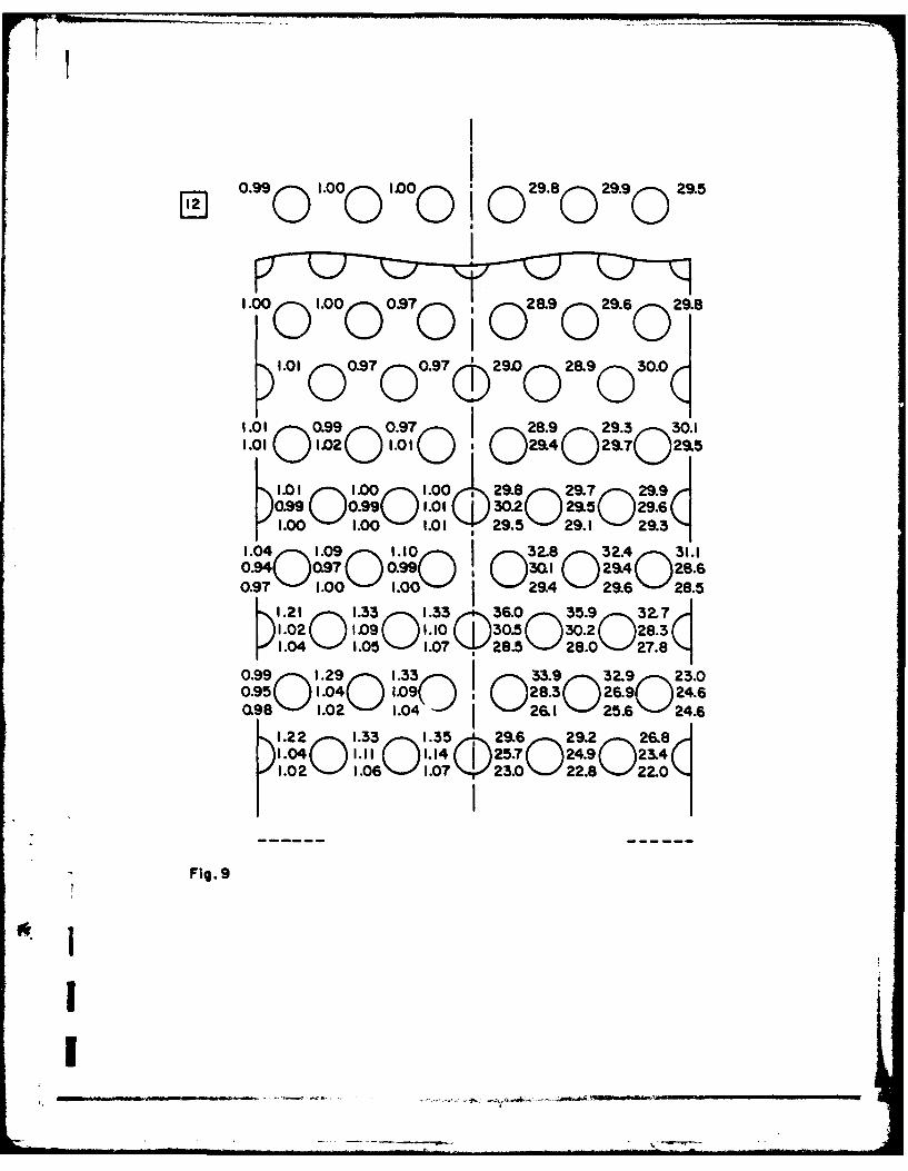
Re - 850 and 8400. Similarly, Figs. 9 and 10 are both for a two-fold enlargement,

with Re = 850 and 8400 respectively. An indication of the extent of the enlarge-

ment is shown by the dashed lines at the bottom of each figure. The direction of

the mainflow is from the bottom to the top of the figure. To facilitate the dis-

cussion of the format, attention may be focused on any one among Figs. 7 - 10, say,

Fig. 7.

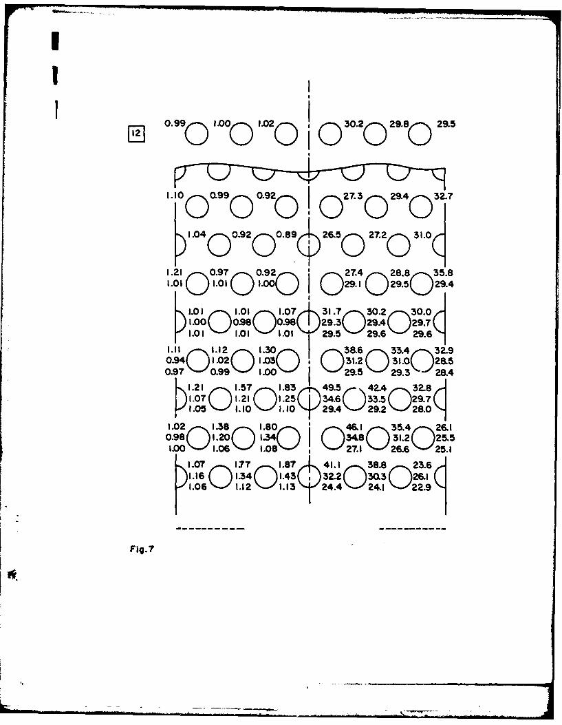
Figure 7 is a plan view of the array, and numbers are inscribed adjacent to

each tube. There are, in fact, two sets of numerical results that are presented,

one set being a Sherwood number ratio and the other set being the Sherwood number

itself. The values of the Sherwood number ratio are inscribed in the left-hand

half of the array while the Sherwood numbers are inscribed in the right-hand half.

The two halves of the array may be thought of as being separated by a symmetry

line which runs parallel to the two sidewalls, midway between them. Because the

area enlargement plates were centered in the cross section (Fig. 2), symmetry

prevailed both with and without enlargement. Any slight data scatter at symmetric

tube locations was averaged out, and the thus-obtained average values are reported.

The Sherwood number ratios that appear in the left-hand half of the figure

will now be explained. Adjacent to each tube, three numbers are generally in-

scribed (at downstream rows, only one or two numbers may appear). The uppermost

of the three numbers pertains to the case where the enlargement occurs at the

inlet face of the tube bundle (i.e., no delivery duct). Similarly, the middle and

j lowermost numbers correspond, respectively, to the cases where the enlargement

I

13

occurs at the upstream end of the intermediate and longest delivery ducts

(Fig. 1).

Each number represents the ratio

Sh (with enlargement) (5)Sh (without enlargement)

where both the numerator and denominator of (5) correspond to the same tube position,

the same delivery duct length, and the same Reynolds number. The Sh values for

the denominator are those of Fig. 6. Note that for the trio of numbers inscribed

adjacent to a particular tube location, the denominators are not quite equal.

The Sherwood number ratios are listed to the left of the tube location to which

they pertain. The listing of the ratios is continued in the downstream direction

until they are more or less equal to unity and then is terminated. The attainment

of this condition is more rapid when the delivery duct is in place, and this explains

the early termination of the listings for those cases.

The format of the Sherwood number listing in the right half of the figure

will now be illuminated. The numbers that appear to the right of each tube loca-

tion are the Sherwood numbers for that location. For each set of numbers, the

upper, middle, and lower entries correspond respectively to enlargement at the tube

bundle inlet face and at the upstream end of the intermediate and longest delivery

ducts. The row-by-row listing for each delivery duct is continued downstream until

a fully developed value is obtained, at which point the listing is terminated.

The reason for presenting both Sherwood number ratios and Sherwood numbers

is that each conveys a different type of information. The Sherwood number ratios

provide a direct measure of whether enlargement enhances or degrades the per-tube

Sherwood number, with ratios larger than one indicating enhancement and ratios below

4one indicating degradation. However, the largest ratios do not correspond to the

d.I

14

largest Sherwood numbers nor do the smallest ratios correspond to the smallest

Sherwood numbers. It is for this reason that the actual Sherwood numbers are also

listed.

The discussion will now be directed to the trends in the Sherwood number ratio.

From an overview of Figs. 7 - 10, it is seen that the ratios in excess of one far

outweigh the ratios that are less than one. Even among the ratios whose values are

less than one, most are only a few percent below, and only two values are less

than 0.9 (0.86 and 0.89, respectively). Therefore, the presence of the enlarge-

ment enhances the tube bundle heat transfer. Furthermore, the larger the enlarge-

ment ratio, the greater is the enhancement, as can be seen by comparing Figs. 7 and

8 with Figs. 9 and 10. The extent of the enhancement is also strongly influenced

by the location of the enlargement, with greater enhancements being encountered when

the enlargement occurs closer to the bundle inlet.

On the other hand, the closer the enlargement to the bundle inlet and the

greater the enlargemet ratio, the larger is the overall nonuniformity of the Sherwood

number ratio in a given row. These intra-row nonuniformities result because the

fluid flow entering the tube bundle is concentrated in the central region of the

inlet cross section. Therefore, in the initial rows of the bundle, lower values

of the Sherwood number ratio are encountered adjacent to the side walls. These

nonuniformities disappear with increasing downstream distance.

However, in the extreme case when the largest enlargement ratio occurs at the

bundle inlet face, a secondary intra-row nonuniformity appears downstream, whereby

the highest Sherwood number ratio in the row occurs adjacent to the side walls

(Figs. 7 and 8). This behavior is consistent with the findings of the flow

visualization studies, where it was noted that overly rapid transverse spreading

I of the flow In the initial rows gives rise to an excess of fluid adjacent to the

side walls in the later rows. The secondary intra-row nonuniformity dies away at

3 sufficient downstream distances.

W

15

The greatest enhancements occur in the first row of the tube bundle. The

extent of the enhancement encountered there increases somewhat with the Reynolds

number and markedly with the enlargement ratio and with closer proximity of the

enlargement to the bundle inlet. It is also interesting to observe that for the

greatest enlargement ratio and closest proximity, concerns about a possible "dead-

water," degraded-Sherwood-number zone directly behind the enlargement step did not

materialize. In Fig. 8, first-row enhancements that exceed a factor of two are in

evidence, and enhancements almost as large occur in the first three rows in both

Figs. 7 and 8.

Significant effects of the enlargement (ten percent or greater) persist to the

eighth row for the four-fold enlargement positioned at the inlet face of the bundle

(Figs. 7 and 8). This deep penetration into the bundle is associated with the just-

discussed secondary fluid flow nonuniformity. For the inlet-positioned two-fold

enlargement, ten percent effects are felt through the fourth row (Figs. 9 and 10).

When the enlargement occurs at the upstream end of the delivery duct, its

effect does not penetrate as far into the bundle as when the enlargement occurs

at the bundle inlet. For example, in the case of the longest delivery duct and a

four-fold enlargement, the effect persists to the third row for Re = 850 (Fig. 7)

and only to the second row for Re = 8400 (Fig. 8). Even shorter penetrations are

in evidence for the two-fold enlargements (Figs. 9 and 10).

The row-by-row progression of the Sherwood number ratios toward a downstream

value of unity is not necessarily monotonic. This is because both the numerator

and denominator Sherwood numbers which comprise the ratio may vary nonmonotonically

from row to row. In particular, in connection with the denominator values,

there is an overshoot which was identified in connection with Fig. 6. The non-

monotonic behavior of the numerator will be discussed shortly.

Attention will now be turned to the Sherwood number values listed in the

right-hand half of Figs. 7 - 10. To identify the main trends, it is useful to

I16

focus on a given enlargement ratio and enlargement positioning and to follow the

Sherwood number from row to row. For the four-fold enlargement at the closest

position, the Sherwood number increases from the first to the third rows, at which

point it attains a maximum and then drops off very sharply, followed by a more gradual

decline. Farther downstream, localized increases occur adjacent to the side walls

as a result of the previously mentioned secondary fluid flow nonuniformity.

For the same enlargement ratio but with the enlargement at the intermediate

position, the maximum is now shared by the second and third rows and is also less

lofty. With the enlargement at the position farthest upstream of the bundle inlet,

the Sherwood number varies monotonically from row to row for Re = 850 but displays

a slight maximum for Re = 8400. The localized Sherwood number increases in the

downstream part of the bundle, which were observed for the close-positioned enlarge-

ment, do not occur when the enlargement is positioned upstream of the bundle inlet.

For the two-fold enlargement and Re = 850 (Fig. 9), an unambiguous maximum

occurs (in the third row) only at the closest positioning of the enlargement.

When Re = 8400 (Fig. 10), maxima (also in the third row) are in evidence for the

first two enlargement positions, but to a lesser extent as the position moves up-

stream of the inlet.

It is relevant to note that the flow visualization photographs, Figs. 4 and

5, foretold the presence of the third-row maxima.

By examining the trio of Sherwood numbers adjacent to each tube location, the

effect of the delivery duct length can be identified. The variations among the

numerical values which constitute a given trio are, of course, greatest in the

initial rows. These variations are impressively large in the presence of the

four-fold enlargement but are more moderate for the two-fold enlargement.

I

I,

- - - - - -~ --

17

PRESSURE DROP RESULTS

As was noted earlier, taps had been installed along the upper wall of the

delivery duct and the test section to enable the measurement of the axial pressure

distributions. For each case (i.e., given delivery duct length, enlargement ratio,

and Reynolds number), the measurements yielded the distribution of (patm - p), where

p is the local pressure at any tap location and patm is the ambient pressure in the

laboratory from which the air was drawn. To obtain a dimensionless representa-

tion, it is appropriate to normalize the aforementioned pressure difference by a

representative velocity head pV2 which is a constant for each case. For this pur-

pose, pV2 was evaluated as

PV 2 min 2 (6)

where , and Amin are defined in the text just prior to equation (3), and p is the

average density in the test section (evaluated at the seventh row).

Figures showing the axial distributions of (patm - P)/ pV2 are available for

each delivery duct length. However, to conserve space, only the figure for the

longest delivery duct need be presented here. As will be shown shortly, this figure

can be used to describe the characteristics of the pressure distributions for the

other delivery ducts.

The pressure distributions are presented in Fig. 11. The data shown there,

all for the longest delivery duct, are parameterized by the enlargement ratio

(1, 2, 4) and by the Reynolds number (850, 8400). On the abscissa, X = 0 cor-

responds to the inlet face of the tube bundle. Axial stations to the left of X - 0

are situated in the delivery duct. For those stations, the abscissa variable is

X/S (S = side of square delivery duct). The tube bundle is situated to the right

of X - 0, and here the row number is used as the abscissa variable (the markers

4for the row numbers are positioned at the centers of the tubes). Owing to the fact

that (patm - p) appears on the ordinate, an increasing trend in the data indicates

Iatm___ _

18

a dropping pressure, while a decreasing trend in the data indicates a pressure rise.

Attention is first turned to the pressure distributions in the tube bundle.

As noted earlier, the first tap is situated midway between the second and third

rows, and subsequent taps are spaced two rows apart. It is seen that for each case,

the data fall on a straight line, which suggests that fully developed conditions

prevail at the third and all subsequent rows. This development is slightly more

rapid than that for the development of the tube-bundle Sherwood number distributions

in the presence of the longest delivery duct. This finding is consistent with the

fact that the pressure distribution develops more rapidly than the velocity field.

The slopes of the three lines for Re - 850 are nearly the same, and similarly for

the three lines for Re = 8400. This characteristic will be employed shortly in the

determination of quantitative pressure-related parameters.

Next, turning to the delivery duct, it may be noted that the flow separation

which takes place at the upstream end of the duct has a marked effect on the pres-

sure distribution, especially at larger enlargement ratios. For the four-fold

enlargement, the pressure drop (shown as a rise in the figure) between the first

and second stations is due to the acceleration of the fluid as it pinches together

downstream of the enlargement plate (i.e., vena contracta effect). Subsequently,

there is a pressure rise (a decrease in the figure) associated with the velocity de-

crease which accompanies the expansion of the fluid into the enlarged cross section.

The pressure rise continues to occur up to the last pressure tap in the delivery

duct, indicating that the expansion has not been completed at that station.

For the two-fold enlargement, the aforementioned vena contracta effect is no

longer in evidence, and the first several taps display a rising pressure. Near

the downstream end of the delivery duct, the pressure appears to be independent

of X. Since the friction-related pressure drop is too small to be seen in the

scale of the figure, the apparent pressure uniformity indicates that the inertia-

related effects spawned by the enlargement have died away, although it is improbable

19

that the flow is fully developed.

Even in the absence of an enlargement plate at the upstream end of the delivery

duct, there is a small zone of separation due to the sharp-edged nature of the

inlet. The pressure recovery downstream of the separated region is reflected by the

first and second data points for the zero-enlargement case. The subsequent data

points are essentially at uniform pressure, reflecting the virtually imperceptible

friction-induced pressure drop. Although not completely fully developed, the flow

arriving at the inlet face of the tube bundle should have experienced substantial

development.

In the intermediate-length delivery duct, the measured pressure distribution

for each case is essentially identical to the first four data points in the cor-

responding delivery-duct pressure distribution of Fig. 11. Furthermore, the tube-

bundle pressure distributions are very similar to those of Fig. 11. For the case

of no delivery duct, the measured tube-bundle pressure distributions are also

similar to the distributions of Fig. 11, except that the data from the first tap

do not lie on the straight lines which pass through the data from the other taps.

The presence of the enlargement gives rise to an additional pressure drop

relative to the no-enlargement case. For the longest delivery duct, the enlargement-

induced incremental pressure drops APincr can be read from Fig. 11 as the vertical

distances between the straight lines appearing in the right-hand portion of the

figure. For example, for Re = 850 and a four-fold enlargement, Ap incr/ PV2 is read

between the uppermost and lowermost straight lines that pass through the circle

data symbols. Values read in this way from Fig. 11 and from similar figures for

the intermediate- and no-delivery-duct cases are listed in Table 1.

The table shows that the incremental pressure drop ranges from 7.5 - 12 velocity

heads for the four-fold enlargement and from 1.3 - 2.5 heads for the two-fold en-

largement. There is no appreciable difference between the results for the longest

20

and intermediate delivery ducts, but there is a significant increase in the pressure

loss when the enlargement occurs at the inlet face of the tube bundle (i.e., no

delivery duct). The table also shows that the smaller the Reynolds number, the

larger is the value of Apincr/ PV2

Fully developed friction factors in the tube bundle can be determined from

least-squares straight lines fitted through the pressure distributions. If

(- dp/dN) represents the pressure drop per row, then the friction factor was evalu-

ated from

f = (- dp/dN)/ pV2 (7)

For a given Reynolds number, the fully developed friction factor was found to be

only slightly affected by the delivery duct or by the enlargement. These variations

were averaged out, yielding f = 0.56 and 0.36, respectively for Re = 850 and 8400.

CONCLUDING REMARKS

The results presented here have shown that the presence of an abrupt cross-

sectional enlargement upstream of a tube bank can give rise to appreciable increases

in the heat transfer coefficient compared with the no-enlargement case. Thus, the

use of heat transfer information from the literature (presumably for no enlargement)

to design a tube bank with upstream enlargement is conservative. On the other hand,

the enlargement causes an additional pressure loss as listed in Table 1, and

these losses should be included in the fluid flow design calculations.

ACKNOWLEDGMENT

The research reported here was performed under the auspices of the Office of

Naval Research.

I!

21

REFERENCES

1. S. Kakac, R. K. Shah, and A. E. Bergles, Low Reynolds Number Flow Heat

Exchangers, Hemisphere, Washington, D.C. (1982).

2. H. H. Sogin, Sublimation from discs to air streams flowing normal to their

surfaces, Trans. ASME 80, 61-71 (1958).

3. A. A. Zukauskas, Heat transfer froi tubes in crossflow. In Advances in Heat

Transfer, Vol. 8, Academic Press, New York (1972).

Table 1

Incremental Pressure Drop Ap incr V Due to Enlargement

Delivery Duct

Re Area Ratio Longest Middle None

850 2 1.4 1.5 2.5

850 4 8.4 8.9 11.9

8400 2 1.3 1.3 1.8

8400 4 7.6 7.5 9.2

--- - -

FIGURE CAPTIONS

Fig. 1 Diagrams of the experimental apparatus

Fig. 2 Enlargement configurations

Fig. 3 Flow visualization pattern when there is no enlargement and no

delivery duct

Fig. 4 Flow visualization pattern in the presence of two-fold enlargement

at the tube-bank inlet

Fig. 5 Flow visualization pattern in the presence of four-fold enlargement

at the tube-bank inlet

Fig. 6 Sherwood number distributions for the no-enlargement case

Fig. 7 Sherwood numbers and Sherwood number ratios for a four-fold

enlargement and Re = 850

Fig. 8 Sherwood numbers and Sherwood number ratios for a four-fold

enlargement and Re = 8400

Fig. 9 Sherwood numbers and Sherwood number ratios for a two-fold

enlargement and Re = 850

Fig. 10 Sherwood numbers and Sherwood number ratios for a two-fold

enlargement and Re = 8400

Fig. 11 Pressure distributions in the longest delivery duct and in the

tube bank

... -I I- v

00000C(n 000000

00000c

IL I)

~~LO

-L)

0TU')

L

0 ~II

CfC

0w

T C#4

Fig. 3

I1

St

Fig. 4

- -

Fig.5

130Re:

120 8400 1

110 T

100

SI) 5%

70 26DELIVERY DUCT

22- a LONGEST

202 4 6 8ROW NUMBER

Fig. 6

I

0,990 ,*00Q 102oD Go 30.2oj 298oc2%

1.10 (D099C)0.92(7 0727.3(7)29.4()32.7

p .04(Z).92(D0.89(~ 26.50C 27.2(7 3l.0q1.21 09 0.92 27* 4 .. ~ 2 8 ,8 35.81.01 1010 10 ! 1090-.ooy U29.IU2.5) 29.4

II

1 501 '- 1.01 1.07 317,.~30.2 30.0A1.00 0.J0*.; 8 (I) 29.3 Q 29A )29.71.01 1.01 1.01( 29.50 29.6 29.6

1 12 130 38.60 33.40 32.90.4 102 1.03 31.2 31.0 28.5

0.970 0 1.0 .9 29.5 29.3 28.4S1.21 o-l .570. .83 ,-..49.5o - 4 . .1.07 .21 1.)i25(I34.6 33.5 (29.7 (1.05 "-1.10 1. 10 29.4 29.2 "~28.0

l4680 35.40 26.1

0: ° °° °" 1°2 Ii3.2 2.

1.0OOJ,).0 6 0 1.0 ) 27 1 26.6 ' 9 25.1) .o 0 177 1.87 ,41.1 38.8 23.6

1.16 -134 .43 ( 3 2 .2 2.1.06 9 0 .12 1.13 4' 24.40 24.10 22.

Fig.7--------------- - 44 -- -

I

H 00"0 O''°O99 o0"6 0 ''°o1

2 0.990 °0*96 ° 0 I 5 0 "" 011

1.|0 0.94 0.90 i 1 0 l|

0.-0o.92 .920 10 109 li 15,.,, o.,o ,.o 0 "030,1.0.92[ 0).92 10 0108 0,71,81.00 1.010 1.00 118 119 118

0.93 "99c0 0 1 120 O0.99 1.00 1.00 1 "I 115 116 114

1.090 1.01 I.18 123 102

)0.97 1.01 .o) 14( 119 0111.03 1.03 1.00 " 130 11

1.07 1 13 1758 0 17 2 1270.8600.991 10 21000.98 1.00 .0 0 1 1 1

1.09 o A4 1.81 213 -. 169 01270.97 1.14 (J1.18 143 (J139 118

1.01 1.0301.0661230 120 120

".00 )1.29 1.48U 147 127 98.71.04 1.13 1.160 0110 01070 98.7

S1.43 - 2.03 ,-- 2.13 158 ,- 150 ,.--. 106 "1.40( 1.69) 1.84(')140 1 ) 129 ),07 tI1.24 1.30 1.34-r 98.0 94.7 9041

FIg. 8

II

0.990 ~ ~ 1.C) 2oo u9.8(0 29.9(0 29.5

1.00o .00 097 28.9 29.6 298

p 1.01 (1).97(1).97 ( 29X)~o 2&9 (j)30.01.010 L0.990 0.97, 0 28.9_29.3 30.1

1.01 .00O 1.00Q' 29. 29.7 29.9

0.9 L 0.990 1,o,1 302( 29.50 29.611.00 1.00 .01 29.5 29.1 29.3

1.04 109 110 O 32.8 324 3110.94Q )0.97 )0.99 ) 301 [29.4 )28.60.97 1.00 1.00"- 0 .2940 29.6 28.5

.21 1.33 ,'. 1.33 36.0 35.9 ,"- 32.71020 109) 1.10 ( 30.5 (30.2 )28.31.04 1.05 1.07 C 28.5 ' 28.0 27.8

0.99-.29 I *,33 33.9 32.9 2300.95 )°1.04 ) .9 ) 28.3 ( 26.9() 24.6098 V 1.02"- 1.04 "- ' 2.1 "25.6 24.6

,.22 1.33 ,-.., 35 0 29. 292 26.8 .

X 102 .06 ' 1.07 23.00 22.8 0 22.0(

---- --------~-

Fig. 9

f

1.010 0.99 1.000.98 0 0.998 1161.00 " 1.01 1.000 116 116 115

ko.99 0.99 , o.02 ,20. ,© ,,i)0.99( 1.00( 1.00() 118 () 117) 1160 '.98 0.99 0.99 1-' 14 "-' 114 I13

1.00 0.*97 1.00 ,-1I 9 0 115 0 118N~l098 1.00 a99 11I7 118 1160.980 1.000 0.99 0 I14 II15 II13

S0.96 1.00 1.01 19 18 131.02 1.03 ) 1.05 124 L 122 121

1.00 1060o11 132 125 I110.94 (0.98 (..? Q 2 9, HQ 40.95 '0.95 16 114 113 113

1.II 1.25, 1.29 ( 152 o 147o 131, 0.96 ().02() 1.05 128 ) 124 1170.99 1.01 '1.00 -116 118 116

1.01 , 1.310 136 ~ 1~~3 1 N 126 97.*51.01 I.13 ()I'I9 ) 118( )1:21 99.60.98 ' 1.03 1.08- 102 -96.8 92.4

1.360 1.45 1.46 108 I10 100h, 1.10 1 ,.35 0 13 99 92.01210 -'1.12 9921.2.1.102 1.20 87.6 83.3 -' 79.9(

Fig. 10

n 9I I q"!

N~ -N -

03

z 4 ~

00

-0

z cj. N -

00 0 d4cac

OD 04 04 a

0 4 al a x<

0 4 a a

0 40

00 N 4 0 3

~Ad4-/(d Wu4Dd)

IN-TUBE HEAT TRANSFER FOR SKEWED INLET FLOW CAUSED BY

COMPETITION AMONG TUBES FED BY THE SAME PLENUM

ABSTRACT

Measurements were made of the axial and circumferential distributions of the

heat transfer coefficient in a tube in which the entering airflow is highly skewed.

The skewness was caused by competition between the test section tube and a paral-

lel tube which draws air from the same plenum chamber. For each of several fixed

Reynolds numbers in the test section tube, the flow imbalance between the competing

tubes was varied parametrically (up to a factor of eighteen), as was the center-to-

center separation distance between the tubes (separation - 1.5, 3, and 4.5 times the

tube diameter). Measurements were also made of the pressure drop, and a visualiza-

tion technique was employed to examine the pattern of fluid flow. Practically sig-

nificant effects of the flow imbalance on the axial distribution of the heat

transfer coefficient were encountered only at the smallest of the investigated inter-

tube spacings. Even for that case, the effects were moderate; for example, the im-

balance-related changes for an imbalance ratio of two did not exceed seven percent.

The experiments involved naphthalene sublimation, and a new technique was developed

for coating the inside surface of a tube with naphthalene.

NOMENCLATURE

A mass transfer surface area

D tube inner diameter

P" diffusion coefficient

f friction factor

- - -. "----

ii

K mass transfer coefficient, equation (1)

K incremental pressure loss coefficientP

Lmod axial length of naphthalene surface per module

AM mass sublimed during data run

Q volumetric flow rate

p pressure at X

p. pressure in plenum

Re Reynolds number, 41i/pnD

ReI Reynolds number of test section tube

Re2 Reynolds number of competing tube

S center-to-center separation

Sc Schmidt number

Sh Sherwood number, KD/F

Sh fully developed Sherwood number for single tubefd ,O

V mean velocity

w airflow rate

X axial coordinate

a angular coordinate

V viscosity

v kinematic viscosity

p density

Pnb naphthalene vapor density in bulk

Onw naphthalene vapor density at wall

T duration of run

Subscripts

1 test section tube

2 competing tube

INTRODUCTION

It is a common occurrence in heat exchange devices that a number of tubes draw

fluid from the same header or plenum so that, in effect, the tubes are competing

among themselves for the available fluid. This occurs, for example, in a shell and

tube heat exchanger where the tube inlets, built into a tube sheet, face upstream

into a plenum chamber from which all tubes draw their fluid. The presence of the

assemblage of tubes and the inherent competition among them plays a decisive role

in shaping the velocity distribution in the fluid entering any given tube. Indeed,

even in the simplest configurations, the tube inlet velocity will differ signifi-

cantly from the classical cases (e.g., either uniform or fully developed profiles)

which are used in both experimental and analytical studies of in-tube heat transfer.

As a case in point, consider a very large plenum supplied with fluid at its

upstream end and bounded at its downstream end by a tube sheet in which the tubes are

arranged on equilateral triangular centers. If the rate of fluid flow drawn into

-each tube is the same, then, owing to symmetry, each inlet is fed by a stream tube

of hexagonal cross section which extends from the face of the tube sheet back into

the plenum. Thus, the velocity profile at inlet corresponds to that for an abrupt

contraction from the hexagonal stream tube to the circular inlet aperture in the tube

sheet and is, clearly, more complex than those of the standard pipe-flow literature.

The next stage of inlet profile complexity--that which is the focus of the

present investigation--is the presence of a high degree of skewness in the profile.

The skewness may result from a number of factors. One of these factors, the one in-

volved in the present experiments, is differences in the rate of fluid flow pass-

ing through the various tubes of the assemblage which draw from the plenum. Thus,

for example, a tube inlet situated next to one which draws a relatively high rate of

*. flow from the plenum will experience an entering velocity distribution that is

skewed in the direction of the high-inflow tube. Furthermore, the extent of the

skewness of the inlet velocity distribution will be accentuated as the degree of the

-- - -- -

2

tube-to-tube flow imbalance increases.

Skewed inlet profiles may also result from the geometry of the plenum or from

the manner in which fluid is supplied to the plenum. In a narrow plenum, the fluid

particles must move on highly curved trajectories in order to reach the various

inlet apertures in the tube sheet. Similarly, fluid supplied to the plenum via a

port in the side of the plenum will also move along trajectories that are highly

curved.

In the presence of a skewed inlet velocity distribution, the separation of the

flow (which occurs at any sharp-edged inlet) will also be skewed, as will the

subsequent reattachment. Moreover, the non-axisymmetric turning of the flow as it

enters the tube should also give rise to a secondary (i.e., circumferential) flow

superposed on the mainflow. These features are not encountered in conventional,

axisymmetric, single-tube flows from which heat transfer results are customarily

obtained for subsequent use in heat exchanger design.

The focus of this investigation is the determination of turbulent pipe-flow

heat transfer coefficients in the presence of skewed inlet velocity distributions.

The approach taken here is to look at the generic problem rather than to be con-

cerned with the large number of specific physical situations where skewness occurs.

To this end, an experimental setup was employed which enabled the skewness to be

varied in a syste-atic manner and which was capable of yielding skewnesses even more

exaggerated than those encountered in normal practice. As indicated earlier, the

inlet-profile skewness studied here is associated with tube-to-tube flow imbalance,

but the results should have qualitative significance for skewness in general.

A schematic view of the experimental arrangement is shown in the upper diagram

of Fig. 1. As seen there, two parallel tubes are set into a large circular plate

(hereafter called the baffle plate) and draw from the open space upstream of the

plate. Each tube was equipped with a downstream-positioned blower, control valve,

and flowmeter (not shown), so that the rate of airflow passing through each could

3

3

be controlled independently.

The experiments were conducted at several fixed Reynolds numbers (i.e., flow

rates) in the test section tube 1 covering the range from 5000 to 44,000. At each

fixed Re1 , the Reynolds number Re2 of the second tube was varied from zero to as

large a value of Re2/Re1 as was permitted by the capabilities of the apparatus (up to

Re2/Re, = 18). The variation of Re2/ReI at a fixed value of ReI served to vary the

degree of skewness of the velocity distribution at the inlet of tube 1. Correspon-

dingly, the measured Nusselt numbers for tube 1 revealed the response of a fixed-

Reynolds-number pipe flow to the degree of flow imbalance and inlet-profile skewness.

Another parameter varied during the course of the investigation was the proximity

of the tubes. If S denotes the center-to-center separation distance and D is the

internal diameter of the tubes, then the proximity may be defined by the O/D ratio.

The investigated values of S/D included 1.5, 3, and 4.5.

Two types of heat transfer coefficients were measured. For each data run,

circumferential-average coefficients were obtained at 21 to 24 axial stations along

the length of the test section tube. For selected runs and at a specific axial sta-

tion, circumferential variations of the coefficient were also measured.

In actuality, the heat transfer coefficients were determined indirectly via

the analogy between heat and mass transfer, with the experiments themselves being

performed with the naphthalene sublimation technique. In this regard, a new pro-

cedure was developed for applying on the inside of a tube a naphthalene coating of

precise dimensions and having a hydrodynamically smooth surface finish.

Two types of fluid flow measurements were made to supplement the heat transfer

experiments. The oil-lampblack flow visualization method was employed to examine

the pattern of fluid flow adjacent to the tube wall, especially in the region where

the separated flow reattaches to the wall. Axial pressure distributions were also

measured to identify the effect of the skewed inlet velocity on the pressure drop.

To the knowledge of the authors, the work described here is the first research

4

involving multiple-tube competing flows. A variety of inlet conditions for single

tubes has been investigated, as reported in {1 - 3).

EXPERIMENTAL APPARATUS

As noted earlier, the experiments were conducted utilizing a pair of parallel

tubes whose upstream ends mated with a large baffle plate and which drew air com-

petitively from the space upstream of the baffle. Whereas the two tubes experienced

strong hydrodynamic interactions, no mass transfer interactions can occur (note

that extraneous, difficult-to-control, thermal interactions would have occurred had

heat transfer experiments been performed). Therefore, only one of the two tubes

(i.e., tube 1) need participate in the mass transfer process, while the other tube

(tube 2) functions only as a fluid flow device. Correspondingly, tube 1 was inter-

nally coated with naphthalene and tube 2 was metallic (aluminum), without naphthalene.

Both tubes had approximately the same internal diameter.

Each of the tubes was part of an independent flow circuit which, along the path

of the airflow, included the tube itself, a flowmeter (one of three calibrated

rotameters), a control valve, and a blower. The blowers were situated in a service

corridor outside the laboratory room, which enabled their discharge, heated by blower

compression and laden with naphthalene vapor, to be vented away from the laboratory.

As a result of this arrangement, the air in the laboratory was free of naphthalene

vapor and at a nearly uniform temperature (about 20 C), maintained by a control

system.

In what follows, the mass transfer test sections will be described first, fol-

lowed by the other apparatus components and the instrumentation.

Mass transfer test sections. Two distinct mass transfer test sections were

employed during the experiments--one to determine the axial distribution of the

mass transfer coefficient and the other for the circumferential distribution. The

axial distribution was, by far, the major focus of the work, and the test section

used in its determination will be described first and in greater detail, with that

.. ....... . . " '+ . I .. . . . - -,- ,, r = : [ ; . .

5

for the circumferential distribution to follow.

The test section used for the axial distribution was of modular design, and a

typical module, flanked by portions of the adjacent upstream and downstream modules,

is pictured schematically in the lower diagram of Fig. 1. As seen there, the

module consists of an outer metallic shell and an inner annular layer of solid naph-

thalene that was implanted by a casting process to be described shortly. The metal-

lic shell is a segment of aluminum tube (i.d. = 4.064 cm, o.d.= 4.826 cm). At one

end of the segment, an internal recess, 0.508 cm long, was formed by cutting away

half the wall thickness. A similar recess was cut into the external surface at the

other end of the module. As can be seen in the diagram, the test section was as-

sembled by mating the internal recess of one module with the external recess of the

adjacent module, with pressure-sensitive tape used to seal the joint against leaks.

The internal diameter D of the cast naphthalene layer was 3.272 cm, while

the axial length Lmod of the naphthalene that was exposed to the airflow varied with

the selected module. For the modules of the type pictured in Fig. 1, three dif-

ferent lengths L were employed, respectively, L /D = 0.388, 0.766, and 1.553.mod mod .3,0.6,ad15.

In the assembly of the test section, the shortest modules were positioned nearest

the inlet, followed by the intermediate modules and then the longest modules. The

specific positions of the respective modules will be apparent from the forthcoming

presentation of results.

The most-upstream module was, necessarily, somewhat different from the others.

The external surface of the metallic wall of the module was machined so that it fit

snugly in an aperture in the baffle plate, and the upstream faces of the module and

the baffle plate were aligned flush. Moreover, the module design was such that its

upstream face was metallic, so that naphthalene sublimation occurred only along the

bore of the module. The L /D ratio for this module was 0.466.mod

All told, as many as twenty-four modules were assembled to form the test

section. Fixtures and supports were provided to ensure the straightness of the

---

6

assembled test section tube.

The technique which was developed for forming a naphthalene coating on the

inside surface of a circular tube will now be described. As a first step, the

naphthalene coating from the preceding data run was removed from each module by

melting and evaporation. Then, a mold was assembled as shown in Fig. 2. The com-

ponents of the mold included the metallic wall of the module, end caps which mated

with the recesses at the respective ends of the metallic wall, and a shaft (diameter -

3.272 cm) which passed through apertures in the end caps and served as the center-

body of the mold. The surface of the shaft had been polished to a mirror-like finish

with a succession of lapping compounds.

Molten naphthalene was poured into the annular cavity between the metallic wall

and the centerbody through an aperture in the wall. Once the naphthalene had

solidified, the shaft and end caps were removed. The resulting surface quality of the

cast naphthalene was comparable to that of the polished shaft. As a final step, the

pouring aperture was sealed with tape to prevent extraneous sublimation. In certain

modules (a total of four), thermocouples were cast into the naphthalene layer, flush

with its interior surface.

Attention is now turned to the test section used for the measurement of the

circumferential distribution of the heat transfer coefficient. In this regard, it

may be noted that the scope of this phase of the investigation was more limited than

that aimed at determining the axial distribution. In particular, the circumferential

measurements were confined to the axial zone 0.472 < X/D < 0.848, which corresponds

to the axial range of the second module of the primary test section that was described

earlier. This is the range in which the maximum heat transfer coefficients were en-

countered,and it was for this reason that it was chosen as the site for the circum-

ferential studies.

In essence, the test section was an aluminum tube with a circular patch of

naphthalene built into its wall. The tube was fabricated from solid aluminum rod

7

stock whose external surface was first turned down to the desired outside diameter

(to fit snugly into the aperture in the baffle plate). Then, a hole, 1.232 cm in

diameter, was drilled radially into the rod at a distance of 2.159 cm from one end.

Finally, the rod was bored axially, resulting in a circular tube with an inner

diameter of 3.272 cm (exactly equal to the i.d. of the test section described earlier).

The naphthalene patch was cast in place by employing the polished shaft that was

used in the casting process for the modules. The shaft was inserted into the bore

of the just-described fabricated tube, thereby blocking off the base of the radial

hole. Molten naphthalene was poured into the open end of the radial hole, into

which a thermocouple was also implanted. After solidification was completed, the

polished shaft was removed, leavinga patch of naphthalene which now formed part of

the surface which bounded the bore of the tube.

The circumferential position of the patch was varied by rotation of the tube,

thereby enabling the detection of the circumferential variation of the transfer

coefficient.

The patch was the only naphthalene surface in its test section that was exposed

to the airflow. Therefore, the measured circumferential variations of the transfer

coefficient reflect circumferential nonuniformities of the velocity field but are

not influenced by upstream mass transfer events. Since the role of the velocity is

expected to be dominant, the measured coefficients should give a true accounting

of the circumferential variations.

Other apparatus components and instrumentation. As already noted, the second

of the two parallel tubes served a hydrodynamic function in that it controlled the

skewness of the velocity distribution at the inlet of the test section tube. The

second tube was of seamless aluminum, with internal and external diameters of

3.239 cm and 4.227 cm, respectively, and a length of 88.9 cm. The tube fit snugly

into an aperture in the baffle plate, and the upstream face of the tube wall was

flush with the upstream face of the baffle. Fourteen taps deployed along the length

8

of the tube were used to make the pressure drop measurements to be described later.

The baffle was also of aluminum, 91.44 cm in diameter and 1.23 cm thick. An

aperture was bored through the plate at its center to accommodate the test section

tube. In addition, four other apertures were machined into the baffle, to be used

one at a time to accommodate the second tube. The three apertures not in use were

closed by aluminum disks, with the joints filled with body putty. The entire upstream

face of the plate was sanded with 600-grit wet or dry paper, with special attention

given to ensure a hydrodynamically smooth surface adjacent to the sealed apertures.

The apertures were deployed along a radial line, with the respective centers at

1.5D, 3D, 4.5D, and 6D from the center of the test section tube (D - internal diameter

of test section tube).

With regard to instrumentation, the four thermocouples implanted in the test

section have already been mentioned. A fifth thermocouple measured the inlet air

temperature. All thermocouples were precalibrated and were read with a programmable,

1 pV datalogger. Airflow rates were measured with calibrated rotameters.

Perhaps the most critical measurement was the determination of the masses of

the individual modules. The amount of naphthalene sublimed during a data run was

determined by differencing the masses of the respective modules measured before and

after the run. For this purpose, a Sartorius ultra-precision, electronic analytical

balance was employed. This balance has a resolving power of 10- 5 g and a capacity

of 166 g. Typical changes of mass during a run were in the 0.05 g range.

Pressure measurements were made with a Baratron capacitance-type, solid-state

pressure meter able to detect 10- 3 mm Hg.

. .

9

FLOW VISUALIZATION

Flow visualization studies were undertaken to gain insights into the effects

of the skewed inlet velocity on the pattern of fluid flow in the initial portion of

the test section tube. These studies were performed utilizing the oil-lampblack

technique. With this technique, a mixture of oil and lampblack powder is brushed

on the surface which bounds the airflow. Ideally, under the action of the forces

exerted by the flow, the mixture will move along the surface, following the paths of

the fluid particles which pass adjacent to the surface. In regions of low velocity

(e.g., stagnation zones, reattachment zones), the mixture will remain stationary,

so that such regions show themselves as black, streak-free zones on the surface.

The technique works best at high Reynolds numbers owing to the relatively high

stresses that exist. At low Reynolds numbers, experience with a variety of flows

has demonstrated that very little can be seen, even if a mixture of high fluidity is

used (low viscosity oil and low particle loading). Furthermore, for vertical or

downfacing surfaces, relatively stiff mixtures have to be utilized to prevent sagging

and runoff, and such stiff mixtures preclude successful visualizations at low Reynolds

numbers. Since the test section tube was horizontal in the present experiments, the

employed mixture had to be stiff enough to avoid sagging along a considerable por-

tion of the tube circumference. These realities restricted the visualization work

to the high Reynolds number range (> 35,000).

To obtain a record of the visualized flow pattern, the inside surface of the

test section tube was covered at its upstream end with white, plasticized contact

paper. Once the oil-lampblack visualization pattern had been formed, the contact

paper was carefully separated from the tube wall and laid flat on a sheet of card-

board for photography.

A photograph of a typical visualization pattern, shown in the aforementioned

laid-out format, is presented in the upper portion of Fig. 3. This photograph

corresponds to a test-section Reynolds number Re, 70,000, to the modest flow

I

10

imbalance Re 2/Re, f 1.26,and to the dimensionless center-to-center separation

distance S/D = 1.5. The right- and left-hand edges of the photo are parallel to the

tube axis, and these edges are in contact with each other during the visualization

experiment. The lower edge corresponds to the inlet edge of the test section, while

the upper edge corresponds to an axial station that is about 2 D from the inlet.

To aid in the interpretation of the pattern, a diagram has been included in the

lower part of Fig. 3 to define angular positions in the test section tube. The dia-

gram shows the inlets of the test section tube and the competing tube. The origin

of the angle 6 is at the point of closest proximity of the two tubes. In terms of 6,

the right- and left-hand edges of the photograph correspond to 6 = 1800.

Prior to the start of the visualization experiment, the entire surface of the

contact paper was covered by a uniformly black film of the oil-lampblack mixture,

so what is seen in the photograph represents a substantial rearrangement. Four dis-

tinct zones are in evidence. There is a relatively straight black band adjacent to

the lower edge (i.e., the tube inlet) and a curved black band somewhat downstream.

Zones contairing streak lines are situated between the two bands and downstream of

the second band.

The visualization pattern indicates that the flow separates at the sharp-edged

inlet of the tube and reattaches to the tube wall along the wavy black band. The

angular variation of the reattachment is a direct consequence of the skewed inlet

velocity resulting from the flow imbalance. In view of the modest imbalance

(Re2 /Re, - 1.26), the extent of the circumferential variation is remarkable. The

0most forward point of the reattachment is at 6 0 , i.e., at the position of nearest

proximity of the tubes, while the most downstream reattachment occurs at 6 = 1800,

(i.e., on the side of the test section away from the competing tube). These results

are consistent with the skewing of the test-section inlet flow in the direction of

the competing tube.

The streak lines upstream of reattachment indicate a wall-adjacent backflow--a

.. ... *

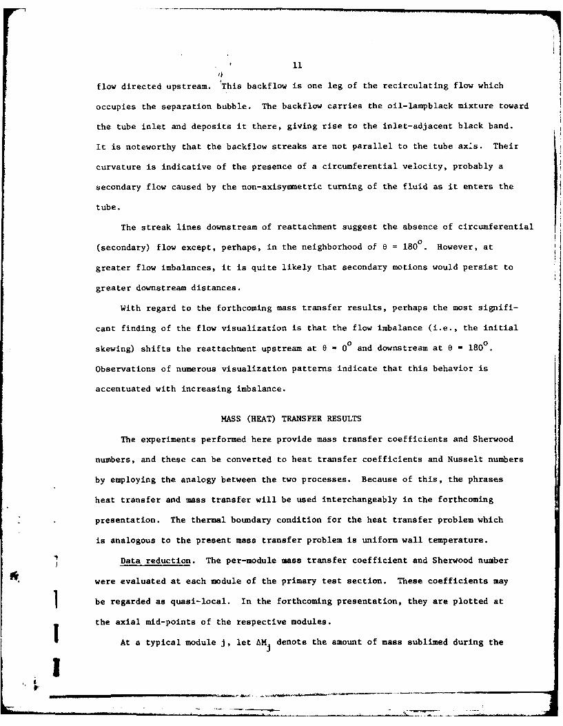
flow directed upstream. This backflow is one leg of the recirculating flow which

occupies the separation bubble. The backflow carries the oil-lampblack mixture toward

the tube inlet and deposits it there, giving rise to the inlet-adjacent black band.

It is noteworthy that the backflow streaks are not parallel to the tube axis. Their

curvature is indicative of the presence of a circumferential velocity, probably a

secondary flow caused by the non-axisymmetric turning of the fluid as it enters the

tube.

The streak lines downstream of reattachment suggest the absence of circumferential

(secondary) flow except, perhaps, in the neighborhood of 8 = 1800. However, at

greater flow imbalances, it is quite likely that secondary motions would persist to

greater downstream distances.

With regard to the forthcoming mass transfer results, perhaps the most signifi-

cant finding of the flow visualization is that the flow imbalance (i.e., the initial

skewing) shifts the reattachment upstream at 6 = 00 and downstream at 6 = 1800.

Observations of numerous visualization patterns indicate that this behavior is

accentuated with increasing imbalance.

MASS (HEAT) TRANSFER RESULTS

The experiments performed here provide mass transfer coefficients and Sherwood

numbers, and these can be converted to heat transfer coefficients and Nusselt numbers

by employing the analogy between the two processes. Because of this, the phrases

heat transfer and mass transfer will be used interchangeably in the forthcoming

presentation. The thermal boundary condition for the heat transfer problem which

is analogous to the present mass transfer problem is uniform wall temperature.

Data reduction. The per-module mass transfer coefficient and Sherwood number

were evaluated at each module of the primary test section. These coefficients may

be regarded as quasi-local. In the forthcoming presentation, they are plotted at

the axial mid-points of the respective modules.

At a typical module J, let AM denote the amount of mass sublimed during the

!ji

12

run time T and A denote the mass transfer surface area. Also, pnw,j and pnb,J

respectively represent the naphthalene vapor den3ities at the wall and in the bulk.

With these, the per-module mass transfer coefficient and Sherwood number are

Kj = (AM /TA )/(Pnw,j - Pnb,j) (1)

Sh = K D/JI (2)

where S is the diffusion coefficient.

Turning to the specifics of the evaluation of K, it may be noted that both AM

and T are measured quantities and A is known from the geometry of the system. The

vapor density pnw at the wall was found from successive application of the Sogin

vapor pressure--temperature relation {4} and the perfect gas law. The measured wall

temperatures were uniform along the test section, so that pnw was the same at all

modules for a given data run.

To find the bulk vapor density pnb at module J, it may first be noted that the

increase in pnb between the inlet and outlet sections of any module m is

(Apnb) m = (AMm /T)/Q (3)

where Q is the volumetric flow rate passing through the module. Then, it follows

thatj-1

nbj nbo + I (APnb)m + h(Apnb) (4)m'nbJ nb~noj (4

The quantity p nb,o is the naphthalene bulk density at the inlet of the test section

tube, which is zero for the present experiments. Also, Q is virtually constant

along the test section (typical variation ft 0.04 percent).

For the Sherwood number evaluation, it is convenient to eliminate the diffusion

coefficient by using the definition of the Schmidt number Sc, which gives

Shj - (K D/v)Sc (5)

For naphthalene diffusion in air, Sc = 2.5 {4. The kinematic viscosity v was

evaluated as that for pure air--consistent with the minute concentrations of the

naphthalene vapor.

.1i'-

. . . . . . .Ii, ,l I i .. .

13

The evaluation of K and Sh for the circuaferentially orientable test section

follows the same pattern as that for each module. The area A that appears in equa-

tion (1) now represents the surface area of the naphthalene patch, while pnb = 0 since

no mass transfer occurs upstream of the patch.

The Sherwood number results will be parameterized by the Reynolds numbers Re

defined in the conventional manner as

Re - 4*/IjwD (6)

in which 4 is the mass flow rate of the air.

Axial distributions of the transfer coefficient. As a prelude to the presen-

tation of the axial distributions, the measured fully developed Sherwood numbers for

single-tube operation will be compared with the literature. For these experiments,

the second-tube's aperture in the baffle plate was sealed. Comparisons were made

over the range from Re - 5000 to 88,000 with the Petukhov-Popov equation (equations

(8 - 23) and (8 - 24) of (5)) and its low Reynolds number extension due to Gnielinski

(6). Agreement to five percent or better was encountered over the entire range,

lending strong support to the present experimental technique.

Axial distributions of the Sherwood number along the test section tube are pre-

sented in Figs. 4 and 5. These results correspond to two-tube operation (with the

single tube as a special case) and to the smallest of the investigated center-to-

center separation distances, S/D - 1.5. Figure 4 conveys results for two fixed

values of the test section Reynolds number, Re1 - 5000 and 9000, while Fig. 5 pre-

sents the corresponding information for Re1 = 22,000 and 44,000.

At each fixed value of Rel, data are plotted for various flow imbalance ratios

Re2 /Re1 = 0 (single-tube operation), 2, 4, ... . Since the maximum attainable value

of Re2 was approximately 88,000, the largest imbalance ratio,' ,18, was achieved at

the smallest Re1 (- 5000). As Re1 increased, the range of the imbalance ratio de-

creased, so that at Re, U 44,000, the largest imbalance ratio was about two. Cor-

respondingly, the successive graphs, starting with Re, - 5000 and proceeding toward

[" ,

14

larger Rel, include fewer data points.

The local Sherwood numbers for all operating conditions at a fixed value of

ReI have been normalized by the measured fully developed Sherwood number correspond-

ing to single tube operation at that Re1 . This quantity is designated as ShV fd,0'

and the ordinates of the graphs are Sh/Shfd,O.

An overall view of Figs. 4 and 5 indicates a common pattern for all the Sherwood

number distributions. Starting with a moderate value adjacent to the tube inlet, the

Sherwood number increases sharply to a maximum, whereupon it decreases, rapidly at

first, and more gradually thereafter, finally approaching the fully developed value.

For all cases, the maximum occurs at the second module, which is centered at

X/D = 0.660.

The aforementioned distribution is characteristic of tube flow with a sharp-

edged inlet, which gives rise to inlet-adjacent separation. The reattachment of the

flow at the tube wall is responsible for the sharp peak in the transfer coefficient,

and the subsequent dropoff of the coefficient is a consequence of the post-reattach-

ment redevelopment of the flow. It is interesting to note that despite the common

occurrence of the sharp-edged inlet, analytical predictions for this configuration

have not appeared in the literature.

In assessing the effects of flow imbalance (i.e., the skewing of the inlet

flow), it is useful to regard the single-tube data (i.e., Re2/Re, f 0, open circles)

as a reference. Relative to that reference, an overview of Figs. 4 and 5 shows

that the imbalance can cause substantial changes in the Sherwood number. However,

a closer inspection reveals that if very large imbalances such as Re 2/Re = 10

and 18 are excluded, then the effects of the imbalance are moderate. For instance,

for Re 2/Re, - 2 and Re, W 9000, there is no axial station at which the imbalance-

related change in Sh exceeds five percent, while for Re1 - 22,000 and 44,000, five

percent (or slightly greater) changes occur at only a few discrete points. Even for

Re1 = 5000 and Re2/Re1 = 2, the largest imbalance-related change is seven percent.

15

In this regard, it may be noted that a factor-of-two flow imbalance is by no means

small when viewed from the standpoint of practice.

Large flow imbalances (Re2/Re1 . 10 and 18) significantly affect the Sherwood

number distribution, both in the immediate neighborhood of the inlet and downstream

of the sharp dropoff which follows reattachment. For example, at Re, - 5000,

deviations of ten percent between the large-imbalance distributions and that for

the single tube persist to X/D - 12. However, with increasing Re1 , the effect

of the imbalance appears to lessen, as suggested by a comparison of the Re 2/Re, = 10

distributions for Re1 . 5000 and 9000.

Another interesting characteristic of the results is that the presence of the

imbalance does not have a universally enhancing or degrading effect on the Sherwood

number. At the first measurement station, the imbalanced flows yield larger Sherwood

numbers than that for the single tube, while the opposite relationship is in evi-

dence at the second and third stations. Thereafter, there is even less regularity

in that the existence of enhancement or degradation at a specific X/D depends on

the magnitude of Re2/Re1 . For the larger Re2/Re1 (10 and 18), enhancement occurs

with regularity in the region downstream of the rapid decrease of the Sherwood

number that follows reattachment.

Certain of the trends noted in the preceding paragraph can be rationalized by

taking cognizance of the shifting of the reattachment line which accompanies an

increase in the flow imbalance ratio, as indicated by the visualization study.

Another factor which may explain the downstream enhancement in evidence at large

values of the ratio is the presence of a secondary flow (i.e., a swirl) induced when

the fluid turns to enter the tube (in a manner similar to a pipe bend).

The data of Figs. 4 and 5 have been brought together in an alternate presen-

tation in Fig. 6 in order to address the question of whether the imbalance-related

effects can be correlated solely as a function of the imbalance ratio Re2/Re1.

5 The figure contains three graphs, respectively for Re2/Re1 W 2, 4, and 10 (lower to

Hill I II-II--------.--, - -.-- ---.-- --- : - - . .

16

upper), and in each graph Sh/Shfd,O data are plotted for various Reynolds numbers.It is evident from the figure that Sh/Shfd,O depends on Re1 as well as on Re2/Re1 .

Overall, at a fixed Re2/Re1, there is a tendency for Sh/Shfd,O to increase with

Rel, which is consistent with the expectation that lower Reynolds number flows are

more sensitive to disturbing influences.

Thus far, the presentation of results has been focused on the closest of the

investigated center-to-center distances, i.e., S/D - 1.5. Attention is now turned

to the effect of increases in S/D. Since the lowest Reynolds number case, Re, f 5000,

is the most sensitive to the flow imbalance, it will be considered first.

In Fig. 7, Sh/Shfd,O distributions for Re1 M 5000 are plotted for S/D = 3

and 4.5, respectively in the lower and upper graphs. If Fig. 4 is kept in mind,

then Fig. 7 indicates a great decrease in the effects of the flow imbalance with in-

creasing S/D. At SID = 3, there is no detectable effect of the Re 2/Re, - 10 flow

imbalance, and even for Re 2/Re, M 18 the deviations of the Sherwood numbers from

the single-tube values are, for the most part, negligible. If the spacing is

increased to S/D = 4.5, then the results for Re 2/Re, = 18 are coincident with those

for Re2/Re1 = 0.

The S/D effect is addressed for larger values of Re1 in Fig. 8, where results

for Re1 = 9000 and 22,000 are plotted for S/D = 3. Here again, the data for the

Re 2/Re1 > 0 cases are indistinguishable from those for Re 2/Re, - 0.

Figures 7 and 8 indicate that even enormous flow imbalances are not felt when

the tubes are moderately far apart. By the same token, if the tubes were to be

positioned much closer together than the S/D - 1.5 separation investigated here,

there could well be a large magnification of the effects of the flow imbalance.

Circumferential distributions of the transfer coefficient. The circumferential

distributions of the Sherwood number, measured by a naphthalene surface patch

centered at X/D = 0.660, are plotted in Fig. 9. The figure consists of four graphs,

respectively for Re1 - 5000, 9000, 22,000, and 44,000. In each graph, data for

.

17

Sh/Sh fd, are plotted as a function of the circumferential position 6, where 6 is

defined in the diagram below the photograph of Fig. 3. The data are parameterizedby the flow imbalance ratio Re 2/Re., with the single tube (Re2/Re, = 0) included

for reference purposes. All the data are for S/D - 1.5.

In appraising the results, it is helpful to recall that 6 = 0 corresponds to

the position of closest proximity of the two tubes, while 6 = 1800 is the position

farthest from the competing tube. It may be noted that uncertainty bars have been

affixed to various of the data points. These bars reflect the range of the data from

multiple repeated runs; in those cases where there are no bars, the repeated runs

gave virtually identical resul-s.

As seen in the figure, the Sherwood number, starting from its value at 6 = 00,

increases to a maximum, whereafter it declines and attains a minimum at 6 = 1800.

Owing to symmetry, the pattern repeats for 1800 < 6 < 3600. Since the number of

circumferential measurement sites was limited, the actual maxima of the respective

distributions may not be quite coincident with the plotted maxima. It is believed,

however, that the true minimum occurs at 6 - 1800.

At high values of the flow imbalance ratio Re 2/Re., the maximum and minimum

of the circumferential distribution are widely separated. As Re 2/ReI decreases, the

extrema tend to come together, and when Re2/Re, - 0, the distribution is circumfer-

entially uniform (within the scatter of the data).

The development of the circumferential variation with increasing Re 2/Re can

be traced to the related shifting of the flow reattachment--in the upstream direction

at 6 = 00 and in the downstream direction at 6 - 1800. Thus, for sufficiently large

Re2/Rel, the reattachment at 6 = 00 lies upstream of the patch location, while for

e - 180 the reattachment occurs downstream of the patch. At these angles, the patch

*. is respectively situated in the (post-reattachment) redevelopment region and in the

(pre-reattachment) separated region. The curved reattachment line (Fig. 3) passes

through the patch site at angular position somewhere between 6 - 00 and 1800,

18

causing the maximum in the distribution curve.

PRESSURE DROP RESULTS

For the pressure drop measurements, the tap-equipped metallic tube was posi-

tioned in the baffle aperture otherwise occupied by the mass transfer test section.

Another metallic tube was employed to establish the flow imbalance.

In all cases, the linearity of the pressure distributionwas established for

X/D > 10. In the linear region, the local pressure p(X) can be related to the

pressure p, in the upstream plenum via the expression

2(p. - p(X))/PV (X/D)f + K (7)p

where f is the friction factor. The quantity K is the incremental pressure lossP

coefficient. It takes account of the losses associated both with the entry of the

flow into the tube and with the hydrodynamic development which occurs within the

tube.

Values of K were determined for both single-tube and imbalanced two-tube opera-p

tion. For the single tube, the measured K values were 1.66, 1.58, 1.53, 1.52, andp

1.52, respectively for Re - 5, 9, 22, 44, and 88 thousand. Flow imbalance was

found to increase Kp but to a remarkably small extent. For example, for Re2 /Re, W 4,

Re, a 22,000, and S/D - 1.5; the K value was only 3.7 percent larger than that

for the single tube. The maximum imbalance effect on K among all of the investi-P

gated cases was about ten percent.

CONCLUDING REMARKS

The present work appears to be the first investigation of turbulent tube-

flow heat transfer and pressure drop in the presence of inlet flow skewness caused

by competition between tubes for fluid drawn from a common plenum. In the execution

i. of the experiments, the test section Reynolds number was fixed at one of several

preassigned values, while the flow imbalance was varied parametrically. The effect

of the center-to-center distance S between the two competing tubes was also

19

investigated, with S/D being varied from 1.5 to 3 to 4.5.

The heat transfer results were determined indirectly by mass transfer measure-

ments utilizing the naphthalene sublimation technique. In this regard, a new

coating procedure was developed which enabled naphthalene to be cast on the inside

of a circular tube. The pattern of fluid flow in the test section tube, just down-

stream of the inlet, was visualized with the oil-lampblack technique. Axial pres-

sure distributions were measured to determine the additional losses due to the

flow imbalance.

Practically significant effects of the flow imbalance on the axial distribu-

tion of the Sherwood number were encountered only at the smallest of the investi-

gated intertube spacings, i.e., S/D - 1.5. Even for that case, the effects were

moderate except at very large imbalances. For example, for a flow imbalance ratio

of two, which is by no means small from the standpoint of practice, the largest

imbalance-related changes did not exceed seven percent.

The pressure drop information was presented in terms of a coefficient which

reflects the losses associated with the entry of the flow into the tube and with its

hydrodynamic development. For all the investigated cases, the imbalance-related

changes in the loss coefficient were less than ten percent.

ACKNOWLEDGMENT

The research reported here was performed under the auspices of the Office

of Naval Research.

REFERENCES

1. Boelter, L.M.K., Young, G., and Iversen, H.W., "An Investigation of Aircraft

Heaters, XXVII--Distribution of Heat Transfer Rate in the Entrance Section of

a Circular Tube," NACA Technical Note, No. 1451, 1948.

2. Mills, A. F., "Experimental Investigation of Turbulent Heat Transfer in the

Entrance Region of a Circular Conduit," Journal of Mechanical Engineering

Science, Vol. 4, 1962, pp. 63-77.

titI

p

20

3. Lau, S. C., Sparrow, E. M., and Ramsey, J. W., "Effect of Plenum Length and

Diameter on Turbulent Heat Transfer in a Downstream Tube and on Plenum-

Related Pressure Losses," ASME Journal of Heat Transfer, Vol. 103, 1981,

pp. 415-422.

4. Sogin, H. H., "Sublimation from Disks to Air Streams Flowing Normal to Their

Surfaces," Trans. ASME, Vol. 80, 1958, pp. 61-71.

5. Karlekar, B. V. and Desmond, R. H., Heat Transfer, second edition, West

Publishing, St. Paul, Minnesota, 1982.

6. Gnielinski, V., "New Equations for Heat and Mass Transfer in Turbulent

Pipe and Channel Flow," International Chemical Engineering, Vol. 16, 1976,

pp. 359-368.

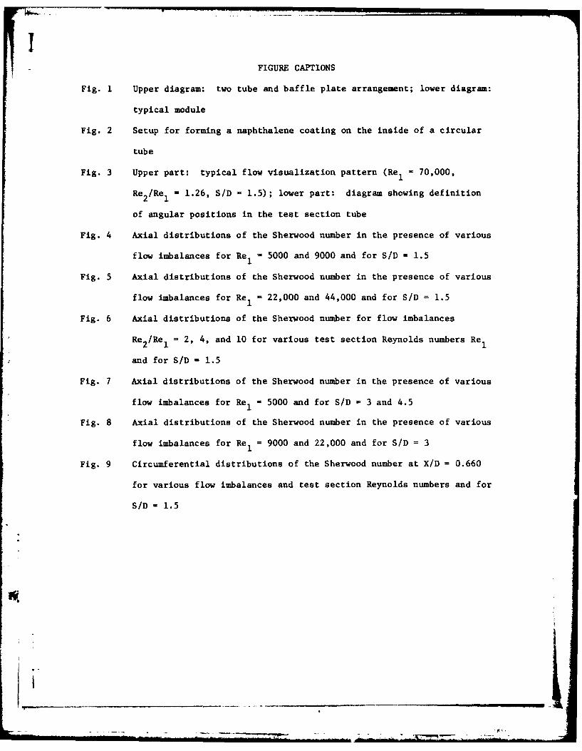
FIGURE CAPTIONS

Fig. 1 Upper diagram: two tube and baffle plate arrangement; lower diagram:

typical module

Fig. 2 Setup for forming a naphthalene coating on the inside of a circular

tube

Fig. 3 Upper part: typical flow visualization pattern (ReI - 70,000,

Re 2/Re, = 1.26, S/D - 1.5); lower part: diagram showing definition

of angular positions in the test section tube

Fig. 4 Axial distributions of the Sherwood number in the presence of various

flow imbalances for Re, - 5000 and 9000 and for S/D = 1.5

Fig. 5 Axial distributions of the Sherwood number in the presence of various

flow imbalances for Re1 = 22,000 and 44,000 and for S/D = 1.5

Fig. 6 Axial distributions of the Sherwood number for flow imbalances

Re 2/Re, = 2, 4, and 10 for various test section Reynolds numbers Re1

and for S/D - 1.5

Fig. 7 Axial distributions of the Sherwood number in the presence of various

flow imbalances for Re1 M 5000 and for S/D = 3 and 4.5

Fig. 8 Axial distributions of the Sherwood number in the presence of various

flow imbalances for Re1 = 9000 and 22,000 and for S/D = 3

Fig. 9 Circumferential distributions of the Sherwood number at X/D = 0.660

for various flow imbalances and test section Reynolds numbers and for

S/D - 1.5

10

012

METALLIC WALL

N APHTHALENE

I Fig. I

..............

a-

D-1-cr 0

a.LLJ

-JL

a.4>

0 CL.Li L0 -

~J oz

00z o 180 0*

I TEST SECTIONj TUBE

Fi.I

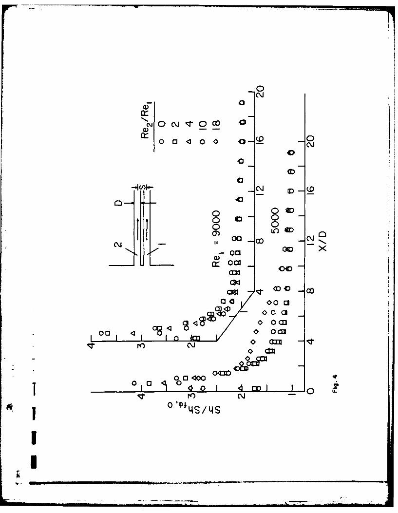
(ITt O 0

N

0 0

o LoO

oaj 01 xocaa

cr- ~ 04D

00 cu0

000

0~~ CLI/L4

0I 00004I 0l

0 a 0000

0) _C 0~

a)(

ID a0 0o

0 0 C

00

cb I

o 'p;I I 0Ij 4 I _

a0

00400000

OT00 00 N0

0D 0

0 43

01

_I -j --. --

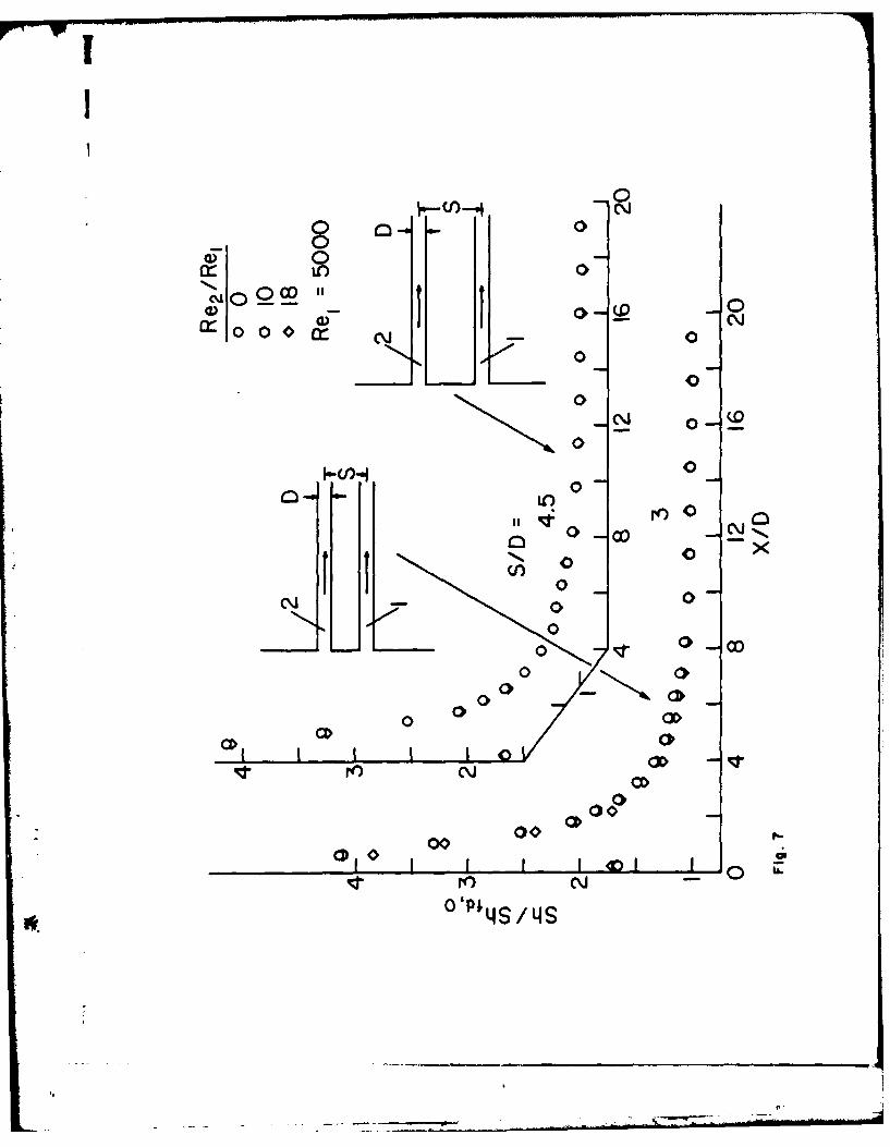
000

0-

C~C

0 o (

0-0

C~j 0

.00

0 a

0 - C00

0'

000

00C I I I I ~

Nl -~

cli -0

00

0~ 0 0

0 0DC~j 0

oC0U 0

Q) 0cr 00 0

0 N 0

N 0Q N 0

0 OD

0000 a

C~j 0

00

CbC

0,P1

-i 0 0 0

(D

o 0~0

o CD

0 0 B0 0zc

0 0

0)LL000t.

0II-

0

} A-

ILI0

LL.

MALDISTRIBUTED-INLET-FLOW EFFECTS ON TURBULENT HEAT TRANSFER

AND PRESSURE DROP IN A FLAT RECTANGULAR DUCT

ABSTRACT

The effects of flow maldistribution caused by partial blockage of the inlet of

a flat rectangular duct were studied experimentally. Local heat transfer coeffici-

ents were measured on the principal walls of the duct for two blockages and for

Reynolds numbers spanning the range between 6000 and 30,000. Measurements were also

made of the pressure distribution along the duct, and the fluid flow pattern was

visualized by the oil-lampblack technique. Large spanwise nonuniformities of the

local heat transfer coefficient were induced by the maidistributed flow. These non-

uniformities persisted to far downstream locations, especially in the presence of

severe inlet-flow maldistributions. Spanwise-average heat transfer coefficients,

evaluated from the local data, were found to be enhanced in the downstream portion

of the duct due to the flow maldistribution. However, at more upstream locations,

where the entering flow reattached to the duct wall follow.ing its separation at

the sharp-edged inlet, the average coefficients were reduced by the presence of the

maldistribution.

NaMENCLATURE

A area of unblocked inlet

Ab blocked area of inlet

A open inlet area with blockage in place

naphthalene-air diffusion coefficient

Dh hydraulic diameter

H duct height, Fig. 1

K local mass transfer coefficient, equation (8)xy

ii

K spanwise-average mass transfer coefficient, equation (10)m

M mass transfer rate per unit length

mass transfer rate per unit area

P duct perimeter

p pressure

p. pressure upstream of inlet

Q volume flow rate, */P

Re Reynolds number, 44/UP

Sc Schmidt number

Shxy local Sherwood number, KxyDh

Sh spanwise-average Sherwood number, KxDh/x

Vi velocity based on inlet cross section, equation (11)

W duct width, Fig. 1

net flow rate in forward direction

x axial coordinate

y transverse coordinate

6 sublimation depth

air viscosity

v air kinematic viscosity

P mean air density

p. air density upstream of inlet

0nb bulk density of naphthalene vapor

Pnw density of naphthalene vapor at wall

Ps density of solid naphthalene

T duration of data run

INTRODUCT ION

Typically, in pipe- or duct-flow experiments, efforts are made to obtain inlet

velocity distributions which either are uniform or are congruous with respect to the

symmetry lines of the cross section. In practice, however, the flow supplied to

the inlet cross section of a tube or duct may be highly maldistributed. This may

occur when the flow is delivered to the duct via a piping system which contains

bends, changes of cross section, valves, blockages, or combinations of these per-

turbing features.

Maldistributed flows may not only be nonuniformly and unsymmetrically dis-

tributed over the inlet cross section, but the maldistribution may set up pockets

of recirculating flow (i.e., backflow) in the duct. In the presence of a maldis-

tributed inlet flow, circumferential variations of the heat transfer coefficient are

virtually a certainty, giving rise to possible hot or cold spots on the duct walls.

In addition, the magnitude of the circumferential-average heat transfer coefficient

may be significantly affected.

In the case of the circular tube, the heat transfer ramifications of a maldis-

tributed inlet flow have been investigated experimentally for a variety of causal

factors (e.g., bends, unsymmetrical blockages, and mixing), and {i - 3} are repre-

sentative of the available literature. On the other hand, the impact of an initial

flow maldistribution on the heat transfer characteristics of rectangular ducts

appears not to have been investigated heretofore. It is the purpose of this paper

to report on an experimental investigation of turbulent heat transfer in a flat

rectangular duct in the presence of an inlet-section flow maldistribution.

The experiments were performed with a high aspect-ratio duct (aspect ratio -

18.3) with a view toward approximating a parallel-plate channel. In planning the

experimental program, it was decided to work with a severe maldistribution. To this

end, the duct inlet configuration illustrated in Fig. 1 was adopted. The figure

is a head-on view looking at the duct inlet from an upstream vantage point. As

2

seen there, the upstream portion of the duct is set into a large baffle plate

such that the exposed end faces of the duct walls are flush with the upstream face

of the baffle. Owing to the presence of the baffle plate and with the system operat-

ing in the suction mode, the entire space upstream of the baffle serves as a plenum

from which flow is drawn into the duct inlet. The duct cross section dimensions

are W and H, width and height, respectively, with W/H - 18.3.

The flow maldistribution was induced by positioning a thin-plate blockage

element as shown schematically in Fig. 1. The presence of the blockage causes the

flow entering the duct to pack to one side of the inlet cross section. Owing to the

inability of the entering flow to turn sharply and fill the space downstream of the

blockage, a low-velocity recirculation zone is set up. On the other hand, the flow

passing through the unconstricted portion of the inlet section streams in a jet-

like manner through the duct, spreading in response to wall friction and momentum

exchange with the recirculation zone.

Experiments were performed for two blockage ratios, respectively 1/4 and 1/2

of the total cross section of the duct. The unblocked case, which can be regarded

as a baseline case against which the maldistribution-affected results may be com-

pared, was investigated earlier {4). For each blockage ratio, experiments were

carried out for four Reynolds numbers spanning the range from 6000 to 30,000.

In addition to the degree of maldistribution (blockage ratio) and the Reynolds

number, the thermal boundary conditions were also varied during the course of the

experiments. In one set of experiments, the two principal walls of the duct

were maintained at the same uniform temperature, while in a second set one of the

principal walls was isothermal and the other principal wall was adiabatic. In all

of the experiments, the side walls were adiabatic.

Local heat transfer coefficients were measured at thirteen points across

the span (i.e., the width) of the duct at each of twenty-one axial measuring sta-

tions. These measurements permitted the evaluation of spanwise-average heat

t,, ~

3

transfer coefficients at the twenty-one axial stations, and it is these spanwise-

average results that will be compared with those for the non-maldistributed flow.

In addition to the heat transfer measurements, two types of fluid-flow-related

results were obtained and will be presented. One of these is the axial pressure

distributions in the presence of inlet-section blockage. The other is the pat-

tern of fluid flow that is created in the duct due to the blockage. The oil-lamp-

black technique was used for the flow visualization.

THE EXPERIMENTS

Test section. As shown in Fig. 1, the test section was made up of two princi-

pal walls which formed the upper and lower bounding surfaces of the flow cross sec-

tion and of two side walls which served as spacers to separate the principal walls.

These walls defined a flow cross section of width W = 8.13 cm (3.20 in.) and height

H = 0.445 cm (0.175 in.), with a resulting hydraulic diameter Dh = 0.842 cm

(0.332 in.). The wall thicknesses shown in the figure are to scale with respect

to H and W. In the streamwise direction, the active length of the test section was

equal to about 2 2Dh.

Instead of heat transfer experiments, the experiments that were actually per-

formed involved mass transfer. According to the analogy between the two processes

(to be discussed later), the measured mass transfer coefficients can be readily

converted to heat transfer coefficients. For the mass transfer studies, eitherone or

both of the principal walls (depending on the desired boundary conditions) were

recessed so as to accommodate a layer of naphthalene which was implanted by a

casting process. On each plate that participated in the mass transfer process,

the spanwise width of the exposed naphthalene surface was precisely equal to the

duct cross-section width W. The streamwise length of the naphthalene surface

was already noted in the preceding paragraph.

Two test setups were employed. In one, one of the principal walls housed a

naphthalene layer which bounded the flow while the other wall was an aluminum plate

4

whose flow-facing surface had been carefully polished. In the other setup, the

flow was bounded by naphthalene surfaces in both walls. According to the heat--

mass transfer analogy, a naphthalene surface corresponds to an isothermal surface

in the counterpart heat transfer experiment, while a metallic surface corresponds

to an adiabatic surface. Thus, the setup where the surfaces of both principal

walls were of naphthalene corresponded to a symmetrically heated channel, while

the setup with only one naphthalene surface corresponded to unsymmetric heating.

The two principal walls which housed the naphthalene were each made from a

solid block of aluminum. Each block was milled all the way through, removing most

of the metal and leaving only an open frame-like structure and internal ribs which

bridged between the frame to give it strength. Naphthalene was cast into the

hollowed-out space such that the naphthalene surface exposed to the airflow was co-

planar with its surrounding metal frame.

The aforementioned machining was performed so that the naphthalene surface

could extend as close as possible to the duct inlet. Correspondingly, the frame

at the upstream end of the test section was narrowed to 0.050 cm (0.020 in.),which

corresponds to a streamwise length = 0.06D . This length of surface did not par-

ticipate in the mass transfer process.

For each data run, a fresh naphthalene layer was cast into each of the mass-

transfer-participating walls, and all portions of the casting except the surface

which interfaces with the airflow were carefully taped to prevent extraneous

sublimation. Upon completion of the casting procedure, the participating walls

were placed in an airtight container and left overnight in the laboratory in order

to attain thermal equilibrium with the room air.

For the determination of the axial pressure distribution in the duct, eight

pressure taps were installed along the spanwise centerline of the aluminum plate

which served as the non-participating principal wall for the unsymuetric mass trans-

fer experiments. The locations of the taps will be evident from the pressure

5

distribution results to be presented later.

Other apparatus components and instrumentation. For the identification of

other components, it is convenient to follow the path of the airflow through the

apparatus. Air drawn from the temperature-controlled laboratory room entered the

test-section duct via the partially blocked inlet. After traversing the axial

length of the duct, the air encountered an abrupt enlargement (area ratio ". 9.5)

as it discharged into a long transition section whose function was to bridge between

the flat rectangular cross section of the test section and the circular piping of

the downstream air-handling system. The external cross-sectional dimensions of

the transition section and the test section were made identical to tacilitate

sealing their interface against leaks.

The piping system leading from the transition section conveyed the air to a

flowmeter (a calibrated rotameter), a control valve, and then to a blower situated

in a service corridor adjacent to the laboratory. The naphthalene-laden blower

exhaust was vented outside the building.

The baffle which framed the inlet of the duct was a 66 cm (26 in.) square

aluminum plate. The 66 x 66 cm face dimensions of the baffle were chosen to be very

large compared with the 8.13 x 0.445 cm dimensions of the duct cross section. Thus,

the fluid flow perceives the duct inlet as an aperture in an infinite wall.

The partial blockage of the inlet was accomplished by affixing a 0.0254-cm

(0.010-in.) thick stainless-steel plate to the face of the baffle by means of

pressure-sensitive tape. The choice of a thin plate was made to ensure a sharply

defined flow separation; the plate was sufficiently thick so as not to deform

under the forces exerted by the airflow. A dial-gage-equipped caliper was used to

ensure the precise positioning of the plate for the desired blockageE

The instrumentation used in the experiments will now be described. The local

mass (heat) transfer coefficients were determined from measurements of the contour

of the naphthalene surface made both before and after each data run. For the

II"-' ... ,. -I I 1i : : i l l

6

contour measurements, the naphthalene test surface, housed in its metal frame,

was positioned, via pins and clamps, on the bed of a coordinate table. The table

permitted controlled, precisely measurable travel in two perpendicular horizontal

directions, and this enabled a sensor tip, similar to that of a dial gage, to be

traversed over the naphthalene surface. The vertical movements of the tip were

converted to electrical signals which were read and printed out by a digital volt--5

meter. The final digit of the printout corresponded to 10 inches.

The outputs of the test-section pressure taps were conveyed by plastic tubing

to a selector switch, the output of which was fed to the terminals of a Baratron

solid-state, capacitance-type pressure meter capable of discriminating 10- 4 mm Hg.

The Baratron output was read with a digital voltmeter.

The temperature of the air entering the test section was measured by an

ASTM-certified 0.10F thermometer. In a slected number of data runs ( 1 10),

a calibrated copper-constantan thermocouple was cast into the naphthalene so that

the thermocouple junction lay in the surface exposed to the airflow. In no case

did the run-average value of the thermometer readings differ by more than 0.10C

(0.20F) from the run-average value of the embedded thermocouple readings. This

difference introduces an uncertainty of no more than one percent in the mass

transfer results.

Flow visualization. As was noted in the Introduction, the flow visualization

was performed using the oil-lampblack technique. According to this technique,

a suitable mixture of oil and lampblack is applied to a surface, which is then

exposed to the airflow whose characteristics are to be studied. Ideally, under the

action of the forces exerted by the fluid, the mixture will move along the surface,

following the paths of the fluid particles that pass adjacent to the surface.

Lampblack is a fine black powder which mixes readily with oil. The fluidity

of the mixture can be regulated by the selection of the viscosity of the oil and

by the proportions of the oil and the lampblack powder. The fluidity has a profound

II

7

effect on the extent of the resolution that can be achieved with the oil-lampblack

technique. A stiff mixture will not respond to low velocities while a very fluid

mixture will be blown away by a high velocity stream so that, in either of these

cases, little information is obtained.

In the present instance, owing to the complexity of the flow, mixtures of differ-

ent fluidities had to be used for different parts of the duct surface in order to

cope with the extremes of high and low velocity. To enhance the visualization, the

mixture was applied to the surface in a variety of patterns. These patterns included

a sequence of dots, one or more parallel lines, or a complete coating of a specific

portion of the surface.

The mixture was applied only to the lower principal wall of the duct, since

sagging and dripping would have occurred had the mixture been applied to the upper

principal wall. For all the visualization runs, the lower wall was covered with

white, plasticized contact paper in order to provide the highest possible contrast

for the black streak lines induced on the surface by the flow. Furthermore, to

permit direct observation of the movement of the oil-lampblack mixture during the

visualization runs, a specially fabricated plexiglass plate was used as the upper

wall of the duct.

Visualization runs were performed for the same range of Reynolds numbers as

that for the mass transfer runs. With the blockage in place, there were pockets

of very low velocity flow. In those regions, the most fluid mixture responded

very sluggishly even at the highest Reynolds number. Therefore, in order to obtain

the clearest possible flow patterns for the blockage cases, all of the detailed

visualization runs were made at the highest Reynolds number, namely, about 30,000.

For the presentation of the observed flow patterns, ink tracings of the streak

*. lines were made by overlaying tracing paper atop the white contact paper used to

coat the duct wall.

1

8

DATA REDUCTION

Two types of mass transfer coefficients were evaluated from the experimental

measurements and will be presented in the next section of the paper. One of these

is the local coefficient K at a position x,y on the principal walls of the duct,xy

where x is the axial coordinate (in the flow direction) and y is the spanwise co-

ordinate (across the width W). The other is the spanwise-average coefficient Kx

at an axial station x. The dimensionless counterparts of these coefficients are

the Sherwood numbers Shxy and Sh x, defined as

Sh -K D/, Sh = D/()xy xy h x x h

and it is these Sherwood numbers that will be employed in the presentation of the

results. In turn, these Sherwood numbers are the analogues of the Nusselt numbers

Nu and Nu,xy x Nu x h D/k, Nu hD/k (2)

xy xy h x x h

For duct flows, it is standard to employ the difference between the wall and

bulk temperatures (concentrations) as 'he basis of the heat (mass) transfer coef-

ficient. In conventional situations where the flow is in the forward direction at

all points of the cross section. (i.e., no recirculation or backflow), the evalua-

tion of the bulk temperature (concentration) in terms of the flow rate 'r and the

heat (mass) added to the flowing fluid is straightforward. For instance, for mass

transfer, if M(x) denotes the mass of naphthalene vapor added to the airflow per

unit time and per unit axial length at x and if Q = /P is the volume flow rate of

the air (P = air density), then

dP nb = M(.)dx/Q (3)

represents the increase in the bulk density (i.e., concentration) of the naphtha-

lene vapor in an axial length dx.

When there is a backflow in a portion of the cross section, as in the present

instance, equation (3),or its heat transfer counterpart, can continue to serve

9

as the definition of the bulk concentration (or temperature) provided that Q is

associated with the net flow rate 4 in the forward direction. In the steady state,

the net forward flow Y, is a constant from cross section to cross section despite

possible differences in the extent of the backflow. Furthermore, with p evaluated

at the axial-mean pressure in the test section, the extreme variation of Q along

the test section was about one percent in the present experiments. Thus, Q will be

regarded as independent of x. With this, equation (3) may be integrated from x - 0

to x = x to yield the bulk concentration of the naphthalene vapor

x=(X) f R(x)dx/Q (4)

0

where the condition pnb = 0 at x = 0 has been employed.

The determination of Pnb(x) from equation (4) requires 4(x) as input.

The surface contour measurements made before and after a data run, when differenced,

yielded the distribution of local sublimation depths 6(x,y) on each participating

wall. With these, the local rates of mass transfer i(x,y) per unit time and unit

surface area follow as

k(x,y) = pS6(x,y)/t (5)

in which ps is the density of solid naphthalene and T is the duration of the data

run. If 1 denotes the upper principal wall and 2 denotes the lower principal wall,

thenW W

it(X) = f (x,y)dy, W(x) f 2(xy)dy (6)1 0l 2 0

and

k(x) I M1(x) + M2(x) (7)

When both walls particpated in the mass transfer process, the contributions of

N1 and 2 to A were within a few percent of each other, while when only one wall

participated, either M1 or M - 0 depending on the test configuration employed.

With the foregoing as background, the evaluation of the mass transfer coef-

ficients will now be described. For the local coefficient Kxy

rA

10

Kxy = ih(x,y)/(p - p (X)) (8)xy nw nb

For one participating wall, i(x,y) was taken directly from equation (5), while in

the case of two participating walls

ih(x,y) = (i(X,y) + ti2 (x,y)) (9)

There were occasional differences between ri and m2 in the five percent range,1 2

but for the most part agreement was in the 2 - 3 percent range. For the spanwise-

average coefficient

Kx = {M(x)/nWl/(pnw - 0nb(x)) (10)

where M(x) is from equation (7), and n = 1 when one wall participates in the mass

transfer process and n - 2 when both walls participate.

The bulk vapor density pb that appears in equations (8) and (10) has been

thoroughly discussed, but pnw' the naphthalene density at the wall, remains to

be evaluated. For this purpose, the naphthalene vapor pressure at the wall was

first computed from the Sogin vapor pressure--temperature relationship {51 and,

with this, 0nb was obtained from the perfect gas law.

The mass transfer coefficients from (8) and (10) were introduced into the

Sherwood number definitions of equation (1). The diffusion coefficient

appearing there was evaluated from the identity = v/Sc, where Sc is the Schmidt

number for naphthalene diffusion in air ( 2.5 {5}), and v is the kinematic

viscosity of air.

Attention will now be turned to the pressure distribution measurements. For

the unblocked inlet, the axial pressure distributions were linear, and the cor-

responding friction factors were in excellent agreement with conventional re-

lationships. These results fulfilled expectations and need not be reported further.

The pressure distributions corresponding to the maldistributed inlet flow

were dominated by inertial effects. Therefore, a pressure loss coeffficient,

rather than a friction factor, is more suitable for their presentation. Also, it

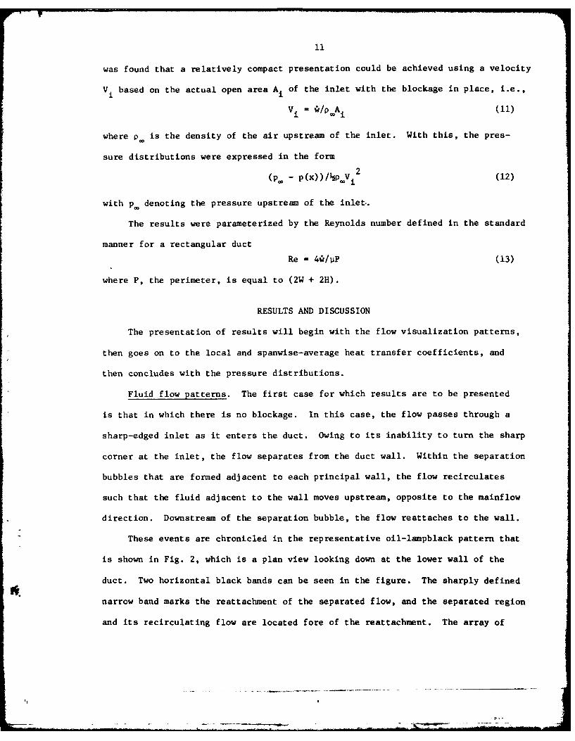
11

was found that a relatively compact presentation could be achieved using a velocity

V based on the actual open area Ai of the inlet with the blockage in place, i.e.,

Si Wv i = */pA i (

where p. is the density of the air upstream of the inlet. With this, the pres-

sure distributions were expressed in the form

2(p. - P(x))/ NPVi (12)

with p. denoting the pressure upstream of the inlet..

The results were parameterized by the Reynolds number defined in the standard

manner for a rectangular duct

Re = 4*/pP (13)

where P, the perimeter, is equal to (2W + 2H).

RESULTS AND DISCUSSION

The presentation of results will begin with the flow visualization patterns,

then goes on to the local and spanwise-average heat transfer coefficients, and

then concludes with the pressure distributions.

Fluid flow patterns. The first case for which results are to be presented

is that in which there is no blockage. In this case, the flow passes through a

sharp-edged inlet as it enters the duct. Owing to its inability to turn the sharp

corner at the inlet, the flow separates from the duct wall. Within the separation

bubbles that are formed adjacent to each principal wall, the flow recirculates

such that the fluid adjacent to the wall moves upstream, opposite to the mainflow

direction. Downstream of the separation bubble, the flow reattaches to the wall.

These events are chronicled in the representative oil-lampblack pattern that

is shown in Fig. 2, which is a plan view looking down at the lower wall of the

duct. Two horizontal black bands can be seen in the figure. The sharply defined

narrow band marks the reattachment of the separated flow, and the separated region

and its recirculating flow are located fore of the reattachment. The array of

12

short vertical lines that populate the separated region are lines of backf low

(i.e., opposite to the mainflow direction). The backflow lines terminate in a

broad black band situated immediately adjacent to the duct inlet. This black

band is the result of an accumulation of the oil-lampblack mixture that was pushed

toward the inlet by the backflow.

It is noteworthy that the reattachment line is, for the most part, straight

and parallel to the duct inlet--indicating that the separation is two-dimensional

over most of the duct width. However, near the inlet and adjacent to the side

walls, there is clear evidence of three-dimensional motions.

Attention may now be directed to Fig. 3, which shows, respectively at the

left and at the right, the flow visualization patterns corresponding to the k and

blocked inlets. In both cases, the blockage is situated at the left side of the

duct inlet. The flow which passes through the unblocked portion of the inlet

creates an inlet-adjacent visualization pattern identical to that already discussed

in connection with Fig. 2, and no further elaboration is needed. The novel features

of Fig. 3 relate, therefore, to the presence of the blockage.

Behind the blockage and over a substantial distance downstream of it, the

velocities are very low and a well-defined recirculation loop is not in evidence.

Rather, the expected recirculating eddy with its clearly defined eye is situated

farther downstream. In the case of the blockage, the eddy appears to have

closed well ahead of the downstream end of the duct and a fully forward flow,

albeit not necessarily fully developed, appears to have been established. For

the blockage case, the eye of the eddy is positioned forward of the exit section,

but the entire eddy has not closed. In neither case is there a tendency for the

entering flow to spread rapidly into the space behind the blockage.

The ramifications of these fluid flow events will be evident during the pre-

sentation of the heat transfer and pressure drop results.

Heat (mass) transfer results. In view of the analogy between the two

13

processes, the phrases heat transfer and mass transfer will be used interchangeably

during the forthcoming presentation. Attention will first be focused on the local

mass (heat) transfer coefficients. Journal space limitations permit only a repre-

sentative sample of the total collection of local-coefficient results to be presented

here, but the full complement of results is available in (6}.

Figure 4 conveys distributions of the local Sherwood r'mber for the case of

the !4 blockage with mass transfer at both principal walls. The figure consists

of eight graphs, each of which corresponds to a specific axial station starting

with the first measurement station x/Dh - 0.22 and ending with the last measurement

station x/Dh = 20.91. These eight stations were selected from among the twenty-one

measurement stations at which data were collected.

In each graph, the local Sherwood number Sh is plotted as a function of thexy

dimensionless spanwise coordinate y/W. The graphs are arranged in two columns.

Atop each column, a line has been drawn to indicate the range of y/W that is

spanned by the inlet-section blockage. Data are plotted for Re = 6000 and 30,000,

which are, respectively, the lowest and highest Reynolds numbers investigated.

Lines have been faired through the data to provide continuity.

Inspection of Fig. 4 reveals that marked spanwise variations in the heat

transfer coefficient are engendered by the maldistributed inlet flow and that re-

siduals of the variations persist even to the downstream end of the duct. The

flow which streams through the unblocked portion of the inlet creates, at

axial stations corresponding to small and intermediate x/Dh , a heat-transfer-

coefficient plateau whose level is very much higher than that of the coefficients in

the low-velocity region behind the blockage. Indeed, the behind-the-blockage

coefficiet.ts are a small fraction of the coefficients encountered in any other

1. portion of the duct.

Detectable increases in the level of the low coefficients begin to appear

at x/Dh 2, and these increases continue at larger x/Dh as the mainflow tends to

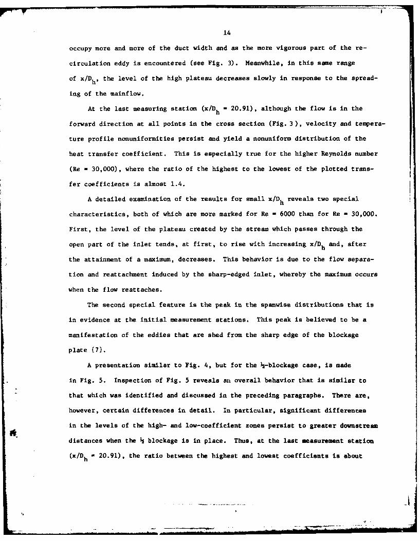
14

occupy more and more of the duct width and as the more vigorous part of the re-

circulation eddy is encountered (see Fig. 3). Meanwhile, in this same range

of x/Dh, the level of the high plateau decreases slowly in response to the spread-

ing of the mainflow.

At the last measuring station (x/Dh = 20.91), although the flow is in the

forward direction at all points in the cross section (Fig. 3), velocity and tempera-

ture profile nonuniformities persist and yield a nonuniform distribution of the

heat transfer coefficient. This is especially true for the higher Reynolds number

(Re = 30,000), where the ratio of the highest to the lowest of the plotted trans-

fer coefficients is almost 1.4.

A detailed examination of the results for small x/Dh reveals two special

characteristics, both of which are more marked for Re - 6000 than for Re - 30,000.

First, the level of the plateau created by the stream which passes through the

open part of the inlet tends, at first, to rise with increasing x/Dh and, after

the attainment of a maximum, decreases. This behavior is due to the flow separa-

tion and reattachment induced by the sharp-edged inlet, whereby the maximum occurs

when the flow reattaches.

The second special feature is the peak in the spanwise distributions that is

in evidence at the initial measurement stations. This peak is believed to be a

manifestation of the eddies that are shed from the sharp edge of the blockage

plate (7}.

A presentation similar to Fig. 4, but for the -blockage case, is made

in Fig. 5. Inspection of Fig. 5 reveals an overall behavior that is similar to

that which was identified and discussed in the preceding paragraphs. There are,

however, certain differences in detail. In particular, significant differences

in the levels of the high- and low-coefficient zones persist to greater downstream

distances when the blockage is in place. Thus, at the last measurement station

(x/Dh 20.91), the ratio between the highest and lowest coefficients is about

15

a factor of two in Fig. 5 compared with about 1.4 in Fig. 4. This significant

spanwise variation of the heat transfer coefficient reflects the nonuniformity

in the fluid flow pattern that is in evidence in the right-hand diagram of Fig. 3.

Also, at certain axial stations, in the low portion of the spanwise distribution,

there is a tendency for the coefficients to tip up near the side wall. This be-

havior may be attributed to the existence of higher recirculation velocities ad-

jacent to the side wall than in the eye of the recirculation eddy.

The highly nonuniform local heat transfer coefficients displayed in Figs. 4

and 5 suggest that hot or cold spots will exist for certain types of heating con-

ditions (e.g., uniform heat flux) due to the maldistributed entering flow.

Attention will now be turned to the spanwise-average mass (heat) transfer

coefficients. This information is conveyed in Figs. 6 - 9, respectively for

Re = 6000, 10,000, 21,000 and 30,000 and for mass transfer at both principal walls.

In each figure, Sh is plotted as a function of the dimensionless axial coordinateK

x/D To provide better resolution in the region just downstream of the inlet,

the abscissa scale has been enlarged in the region 0 < x/Dh < 1. Three sets of

data are plotted in each figure corresponding to the blockage ratios 0 (no blockage),

, and . Curves have been faired through the data for continuity.

All of the axial distributions of the Sherwood number presented in Figs. 6 - 9

share a common shape. Starting at the first measurement station, the transfer

coefficients rise sharply to a maximum and then drop off, rapidly at first and

then more and more gradually. In the far downstream region, the coefficients for

the no-blockage case tend to a fully developed value, while those for the

blockage cases continue to vary slowly.

As was noted earlier, the rise of the transfer coefficient just downstream

of the inlet and the attainment of a maximum is related to the reattachment of the

separated entering flow. The subsequent dropoff is the result of the hydrodynamic

and thermal development processes operating on the reattached flow. There is an

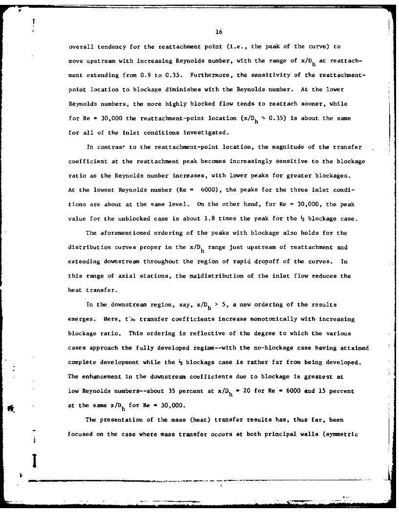
V

16

overall tendency for the reattachment point (i.e., the peak of the curve) to

move upstream with increasing Reynolds number, with the range of x/Dh at reattach-

ment extending from 0.9 to 0.35. Furthermore, the sensitivity of the reattachment-

point location to blockage diminishes with the Reynolds number. At the lower

Reynolds numbers, the more highly blocked flow tends to reattach sooner, while

for Re = 30,000 the reattachment-point location (x/Dh '\ 0.35) is about the same

for all of the inlet conditions investigated.

In contras* to the reattachment-point location, the magnitude of the transfer

coefficient at the reattachment peak becomes increasingly sensitive to the blockage

ratio as the Reynolds number increases, with lower peaks for greater blockages.

At the lowest Reynolds number (Re = 6000), the peaks for the three inlet condi-

tions are about at the same level. On the other hand, for Re = 30,000, the peak

value for the unblocked case is about 1.8 times the peak for the blockage case.

The aforementioned ordering of the peaks with blockage also holds for the

distribution curves proper in the x/Dh range just upstream of reattachment and

extending downstream throughout the region of rapid dropoff of the curves. In

this range of axial stations, the maldistribution of the inlet flow reduces the

heat transfer.

In the downstream region, say, x/Dh > 5, a new ordering of the results

emerges. Here, t'it transfer coefficients increase monotonically with increasing

blockage ratio. This ordering is reflective of the degree to which the various

cases approach the fully developed regime--with the no-blockage case baving attained

complete development while the blockage case is rather far from being developed.

The enhancement in the downstream coefficients due to blockage is greatest at

low Reynolds numbers--about 35 percent at x/Dh = 20 for Re = 6000 and 15 percenthi

at the same x/Dh for Re = 30,000.

The presentation of the mass (heat) transfer results has, thus far, been

focused on the case where mass transfer occurs at both principal walls (symmetrici

17

heat transfer). The results for the case in which only one of the walls actively

participates are essentially coincident (within data scatter) with those already

presented for x/D values up to about five and, in some instances, beyond. This

is as it should be, reflecting the independence of the transfer processes at the

two principal walls until the respective boundary layers have met. Thereafter,

the coefficients for the unsymmetric-transfer case tend to lie below those for

symmetric transfer. In the absence of blockage, the deviations are about seven

percent. For the blockage cases, the deviations are less regular, ranging from

two to ten percent depending on the blockage ratio and Reynolds number. This

irregularity is probably reflective of the non fully developed nature of the flow

and temperature fields.

Pressure distributions. As noted earlier, the pressure drop results cor-

responding to the unblocked inlet are in accord with the literature and need not

be presented here, so that attention will be focused solely on the blockage-

related pressure distributions. These results, expressed in terms oi the pressure

loss coeffficient of equation (12), are plotted as a function of x/Dh in Fig. 10.

The figure consists of four tiers of graphs, one for each of the investigated

Reynolds numbers. In interpreting the results, it should be noted that decreasing

values of p(x) give rise to increasing values of the loss coefficient, while in-

creasing p(x) (i.e., a pressure recovery) causes the loss coefficient to decrease.

From Fig. 10, it is seen that all the pressure distributions for the

blockage share a common pattern, while those for the blockage share a seemingly

different ccmmon pattern. For the blockage, a slight friction-related pressure

drop in the x/Dh range from five to ten is followed by a pressure recovery which

results from the spreading of the mainflow (see Fig. 3). Near the downstream

end of the duct, the pressure recovery is completed and friction-related pressure

drop is about to take over.

The pressure distribution for the blockage case is actually a shifted and

- -------- "-

18

amplified version of that for the blockage case. The small initial pressure

drop for the k blockage is shifted downstream and enlarged (by inertial losses)

for the blockage, and a similar shift occurs for the region of pressure recovery.

The duct is not sufficiently long to enable the pressure recovery to be completed

for the blockage case.

CONCLUDING REMARKS

The analogy between heat and mass transfer has been firmly established on

theoretical grounds for laminar flow and for turbulent flows where the eddy dif-

fusivities for heat and mass are equal {81. Recent empirical confirmation of the

analogy for flows with separated regions has been provided by naphthalene sublima-

tion experiments at Minnesota with cylinders and spheres in crossflow. An even

more convincing demonstration that the analogy is viable in separated flows was

made in naphthalene simulation experiments of a tube bank in crossflow.

In accordance with the analogy, the Sherwood number results presented in

Figs. 4 - 9 and in {6) can be regarded as Nusselt numbers corresponding to a

Prandtl number of 2.5 (equal to the Schmidt number for naphthalene sublimation in

air). These Nusselt number results can then be employed for other Prandtl numbers

using the conventional Prm power-law scaling, where m may be selected between

1/3 and 0.4.

The results presented here have demonstrated that spanwise nonuniformities

in the local heat transfer coefficient induced by flow maldistribution at the

inlet can persist to far downstream locations. The downstream persistence of

the spanwise nonuniformities was found to be greater with a more extreme inlet-

flou maldistribution. Higher spanwise-average heat transfer coefficients were

encountered in the downstream region of the duct due to the flow maldistribution.

However, at more upstream locations, where the entering flow reattaches to the

duct wall following its separation at the sharp-edged inlet, the spanwise-average

coefficients for the maldistributed flows are lower.

19

ACKNOWLEDGMENT

This research was performed under the auspices of the Power Program of the

Offirz of Naval Research.

REFERENC ES

1. Mills, A. F., "Experimental Investigation of Turbulent Heat Transfer

in the Entrance Region of a Circular Conduit," Journal of Mechanical Engineering

Science, Vol. 4, 1962, pp. 62-70.

2. Koram, K. K. and Sparrow, E. M., "Turbulent Heat Transfer Downstream

of an Unsymmetric Blockage in a Tube," Journal of Heat Transfer, Vol. 100,

1978, pp. 588-594.

3. Sparrow, E. M. and Kemink, R. G., "The Effect of a Mixing Tee on Turbulent

Heat Transfer in a Tube," International Journal of Heat and Mass Transfer, Vol. 22,

1979, pp. 909-917.

4. Sparrow, E. M. and Cur, N., "Turbulent Heat Transfer in a Symmetrically

or Asymmetrically Heated Flat Rectangular Duct with Flow Separation at Inlet,"

Journal of Heat Transfer, Vol. 104, 1982, pp. 82-89.

5. Sogin, H. H., "Sublimation from Disks to Air Streams Flowing Normal

to their Surfaces," Trans. ASME, Vol. 80, 1958, pp. 61-71.

6. Cur, N., "Local Turbulent Heat Transfer Coefficients in a Symmetrically

or Asymmetrically Heated Flat Rectangular Duct with Either Uniform or Nonuniform

Inlet Velocity," Ph.D. Thesis, Department of Mechanical Engineering, University

of Minnesota, Minneapolis, Minnesota, 1982.

7. Beavers, G. S. and Wilson, T. A., "Vortex Growth in Jets," Journal of

Fluid Mechanics, Vol. 44, 1970, pp. 97-112.

8. Eckert, E.R.G., "Analogies to Heat Transfer," in Measurement Techniques

*. in Heat Transfer, edited by E.R.G. Eckert and R. J. Goldstein, Hemisphere

Publishing, Washington, D.C., 1976.

!II

- - --%-

FIGURE CAPTIONS

Fig. 1 Duct inlet configuration

Fig. 2 Flow visualization pattern corresponding to a blockage-free

inlet (Re = 21,000)

Fig. 3 Flow visualization patterns corresponding to the and inlet

blockages, left- and right-hand diagrams, respectively

Fig. 4 Spanwise and axial distributions of the local Sherwood number

for the ; blocked inlet

Fig. 5 Spanwise and axial distributions of the local Sherwood number

for the blocked inlet

Fig. 6 Axial distributions of the spanwise-average Sherwood number,

Re = 6000

Fig. 7 Axial distributions of the spanwise-average Sherwood number,

Re = 10,000

Fig. 8 Axial distributions of the spanwise-average Sherwood number,

Re = 21,UO0

Fig. 9 Axial distributions of the ....ise-average Sherwood number,

Re = 30,000

Fig. 10 Pressure distributions corresponding to the A and inlet

blockages

cn

3: La0w 400-

AD-A724 017 STUDIES OF HEAT TRANSFER IN C0OMPLEX INTERNAL FLOWS(U)MINNESOTA UNIV MINNEAPOLIS DEPT OF MECHANICALENGINE ERING E M SPARROW JAN 83 NOOO14-79-C 0621

NChSIFE h S I O G3 N

*mooEd)

l1low

* MICROCOPY RESOLUTION TEST CHART

NATIONAL BURE AU OF STANDARDS-1963-A

Fig.' 2

Fig.3

BxLOCKAGE B2LOCKAGE

400- ~ 0.22 -0

4 0 0

200

30, 00010200 Re= 22

400 ~ -000

100 200

200- 0.45 6.00 100

0h~ 0 L " 3---301-

400-0820

00

4007 200

y/W /

FIG. 4

BOCKAGE BOCKAGE

Rem400- x/Dh= 2.8200

0.22 30,000200-60 100

I 0

030 0400- 0

0.45 60

20:- 100

4004 20000C3C]C--C-i

0 0400- 0

0.8 120

200- 0

0 00

0Y/W 10y/W

it FIG. 5

CNN

44o0 NL 0

4 O O IUIt

Ii~

'IO

o CC

0 0

o i0

00

0 Ip

I'3

mao

IUgI

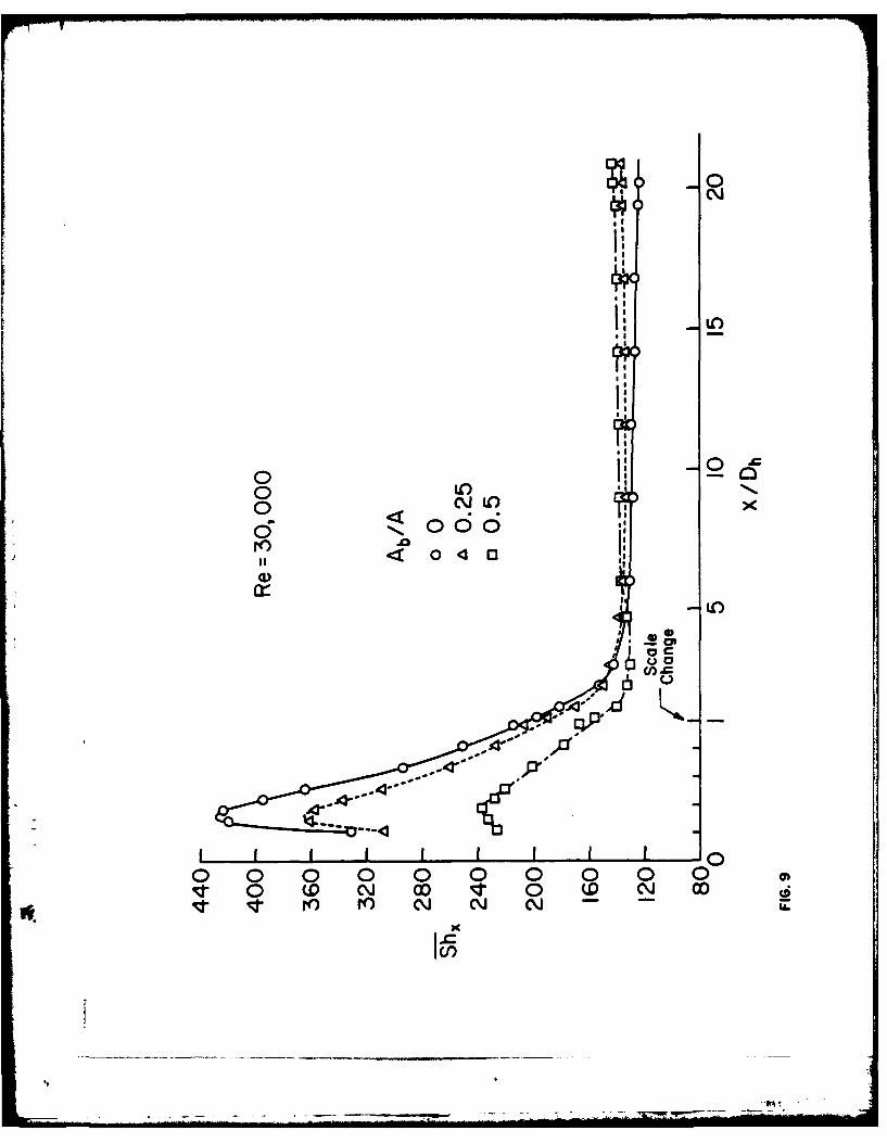
00

0 4 4

.11

0 wj IN O io o Il) Cj Cj I

0c')

LOo 0 00o 0 0 oo LC(I) 0 0 0

oOR (P

2

'Acd (z/I)

()( -- 00d i i nu

DISTRIBUTION LIST

HEAT TRANSFER

One copy exceptas noted

Mr. M. Keith Ellingsworth 5Power ProgramOffice of Naval Research800 N. Quincy StreetArlington, VA 22203

Defense Documentation Center 12Building 5, Cameron StationAlexandria, VA 22314

Technical Information Division 6Naval Research Laboratory4555 Overlook Avenue SWWashington, DC 20375

Professor Paul MartoDepartment of Mechanical EngineeringUS Naval Post Graduate SchoolMonterey, CA 93940

Professor Bruce RankinNaval Systems EngineeringUS Naval AcademyAnnapolis, MD 21402

Office of Naval Research Eastern/Central Regional Office

Bldg 114, Section D666 Summer StreetBoston, Massachusetts 02210

Office of Naval Research Branch Office536 South Clark StreetChicago, Ill. 60605

Office of Naval ResearchWestern Regional Office1030 East Green StreetPasadena, CA 91106

. Mr. Charles Miller, Code 05R13Crystal Plaza i6Naval Sea Systems CommandWashinton, DC 20362

I,U, S

Heat Exchanger Branch, Code 5223National Center #3Naval Sea Systems CommandWashington, DC 20362

Mr. Ed Ruggiero, NAVSEA 08National Center #2Washington, DC 20362

Dr. Earl Quandt Jr., Code 272David Taylor Ship R&D CenterAnnapolis, MD 21402

Mr. Wayne Adamson, Code 2722David Taylor Ship R&D CenterAnnapolis, MD 21402

Dr. Win AungHeat Transfer ProgramNational Science FoundationWashington, DC 20550

Mr. Michael PerlsweigDepartment of EnergyMail Station E-178Washington, DC 20545

Dr. W.H. jheilbahrChief, Energy Conservation BranchDept. of Energy, Idaho Operations Office550 Second StreetIdaho Falls, Idaho 83401

Professor Ephriam M. SparrowDepartment of Mechanical EngineeringUniversity of MinnesotaMinneapolis, Minnesota 55455

Professor J.A.C. HumphreyDepartment of Mechanical EngineeringUniversity of California, BerkeleyBerkeley, California 94720

Professor Brian LaunderThermodynamics and Fluid Mechanics DivisionUniversity of ManchesterInstitute of Science & TechnologyP088 Sackville StreetManchester M6OQD England

Professor Shi-Chune YaoDepartment of Mechanical EngineeringCarnegie-Mellon UniversityPittsburgh, PA 15213

Professor Charles B. WatkinsChairman, Mechanical Engineering DepartmentHoward UniversityWashington, DC 20059

Professor Adrian BejanDepartment of Mechanical EngineeringUniversity of ColoradoBoulder, Colorado 80309

Professor Donald M. McEligotDepartment of Aerospace and Mechanical EngineeringEngineering Experiment StationUniversity of Arizona 85721

Professor Paul A. LibbyDepartment of Applied Mechanics and Engineering SciencesUniversity of California San DiegoPost Office Box 109La Jolla, CA 92037

Professor C. Forbes Dewey Jr.Fluid Mechanics LaboratoryMassachusetts Institute of TechnologyCambridge, Massachusetts 02139

Professor William G. CharacklisDept. of Civil Engineering and Engineering MechanicsMontana State UniversityBozeman, Montana 59717

Professor Ralph WebbDepartment of Mechanical EngineeringPennsylvania State University208 Mechanical Engineering Bldg.University Park, PA 16802

Professor Warren RohsenowMechanical Engineering DepartmentMassachusetts Institute of Technology77 Massachusetts AvenueCambridge, Massachusetts 02139

Professor A. Louis LondonMechanical Engineering DepartmentBldg. 500, Room 501BStanford UniversityStanford, CA 94305

Professor James G. KnudsenAssociate Dean, School of EngineeringOregon State University219 Covell HallCorvallis, Oregon 97331

Professor Arthur E. BerglesMechanical Engineering DepartmentIowa State UniversityAmes, Iowa 50011

Professor Kenneth J. BellSchool of Chemical EngineeringOklahoma State UniversityStillwater, Oklahoma 74074

Dr. James LorenzComponent Technology DivisionArgonne National Laboratory9700 South Cass AvenueArgonne, Illinois 60439

Dr. David M. EissenbergOak Ridge National LaboratoryP.O. Box Y, Bldg. 9204-1, MS-OOak Ridge, Tennessee 37830

Dr. Jerry TaborakTechnical DirectorHeat Transfer Research Institute1000 South Fremont AvenueAlhambra, CA 91802

Dr. Simion KuoChief, Energy SystemsEnergy Research LaboratoryUnited Technology Research CenterEast Hartford, Connecticut 06108

Mr. Jack YampolskyGeneral Atomic CompanyP.O. Box 81608San Diego, CA 92138

Mr. Ted CarnavosNoranda Metal Industries, Inc.Prospect DriveNewtown, Connecticut 06470

Dr. Ramesh K. ShahHarrison Radiator DivisionGeneral Motors CorporationLockport, New York 14094

Dr. Ravi K. SakhujaManager, Advanced ProgramsThermo Electron Corporation101 First AvenueWaltham, Massachusetts 02154

Mr. Doug MarronEngine R&D Branch, Code 5231NC #4Naval Sea Systems CommandWashington, D.C. 20362(Tel 202-692-6874)

Mr. Richard S. CarltonDirector, Engines Division, Code 523NC #4Naval Sea Systems CommandWashington, D.C. 20362(Tel. 202-692-6868)

Mr. Richard F. WyvillEngine Design Branch, Code 5232NC #4Naval Sea Systems CommandWashington, D.C. 20362(Tel 202-692-6931)

Mr. Walter RitzCode 033CNaval Ships Systems Engineering StationPhiladelphia, Pennsylvania 19112(Tel. 215-755-3841)

Dr. Simion KuoUnited Tech. Res. CenterSilver LaneEast Hartford, Conn. 06108(Tel. 203-727-7258)

Mr. T.M. HerderBldg. 464-G2General Electric Co.1100 Western Ave.Lynn, Massachusettes 01910(Tel. 617-594-3360)

Mr. Ed StrainAiResearch of ArizonaDept. 76, Mail Stop 301-2P.O. Box 5217Phoenix, Arizona 85010(Tel 602-267-2797)

Mr. Norm MclntireSolar Turbines International2200 Pacific Hwy.

U. San Diego, CA 92101(Tel. 714-238-6527)

I_ : . : = . - . i .. , ' - - . .-

Mr. Robert W. PerkinsTurbotec Products, Inc.533 Downey DriveNew Britain, Connecticut 06051

Dr. Keith E. StarnerYork Division, Borg-Warner Corp.P.O. Box 1592York, PA 17405

Mr. Peter WishartC-E Power SystemsCombustion Engineering, Inc.Windsor, Connecticut 06095

Mr. Henry W. BraumManager, Condenser Engineering DepartmentDelavalFront StreetFlorence, New Jersey 08518

Dr. Thomas RabasSteam Turbine-Generator Technical Operations DivisionWestinghouse Electric CorporationLester BranchP.O. Box 9175 N2Philadelphia, PA 19113

ItI

I.1