US Army Corpsof Engineers 0Construction Engineering TECHNICAL REPORT M-354Research Laboratory July 1984

AD-A14 685

THE EFFECT OF FLUIDS ON WAVEGUIDES BELOW CUTOFFPENETRATIONS AS RELATED TO ELECTROMAGNETICSHIELDING EFFECTIVENESS

byMichael K. McInemeyScott RayRay McCormackSteve CastilloRaj Mittra

Q..

LAJ

Approved for public release; distribution unlimited.

8 4 08 '* u6O

The contents of this report are not to be used for advertising, publication, otpromotional purposes. Citation of trade names does not constitute anofficial indorsement or approval of the use of such commercial products.The findings of this report are not to be construed as an official Department Sof the Army position, unless so designated by other authorized documents.

DESTROY THIS REPORT WHEN IT IS NO I ONGER NEEDEDDO NOT RETURN IT TO THE ORIGIN,4 TOR

_

UNCLASSIFIEDSECURITY CLASSIFICATION OF THIS PAGE (When Data Entered)

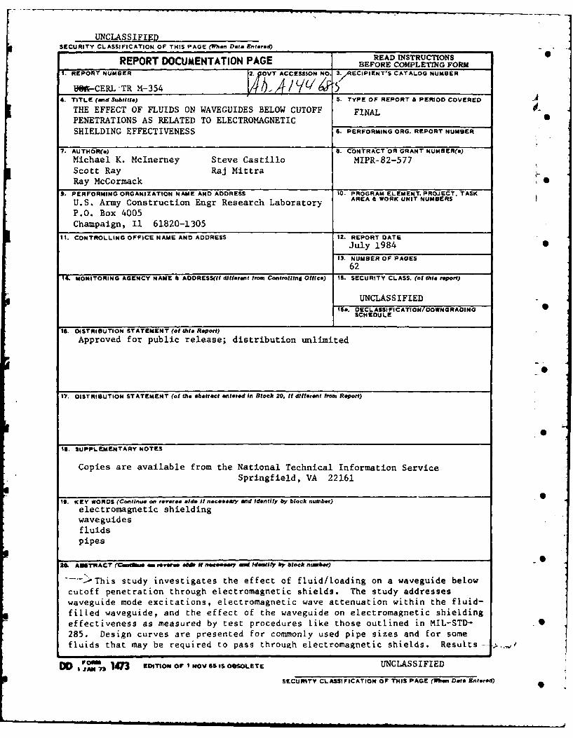
REPORT DOCUMENTATION PAGE READ INSTRUCTIONS 0BEFORE COMPLETING FORM

tREPORT NUMBER 12. POVT ACCESSION NO. 3. ECIPIENT'S CATALOG NUMBER

VOIV-CERL TR M-354 w / (/~4. TITLE (and Subtitle) 5. TYPE OF REPORT & PERIOD COVERED 4

THE EFFECT OF FLUIDS ON WAVEGUIDES BELOW CUTOFF FINAL -PENETRATIONS AS RELATED TO ELECTROMAGNETIC SSHIELDING EFFECTIVENESS 6. PERFORMING ORG. REPORT NUMBER

7. AUTHOR(,) S. CONTRACT OR GRANT NUMBER( )

Michael K. Mclnerney Steve Castillo MIPR-82-577

Scott Ray Raj MittraRay McCormack

S. PERFORMING ORGANIZATION NAME AND ADDRESS 10. PROGRAM ELEMENT, PROJECT, TASK

U.S. Army Construction Engr Research Laboratory AREA & WORK UNIT NUMBERS

P.O. Box 4005Champaign, Ii 61820-1305

II. CONTROLLING OFFICE NAME AND ADDRESS 12. REPORT DATE

July 1984 0

13. NUMBER OF PAGES

6214. MONITORING AGENCY NAME & AOORESS(II different from Controlling Office) 15. SECURITY CLASS. (of this report)

UNCLASSIFIEDISa. DECLASSIFICATON/DOWNGRAOING

SCHEDULE

16. DISTRIBUTION STATEMENT (of thle Report)

Approved for public release; distribution unlimited

17. DISTRIBUTION STATEMENT (of the abaract entered In Block 20, It different from Report)

Is. SUPPLEMENTARY NOTES

Copies are available from the National Technical Information ServiceSpringfield, VA 22161

I. KEY WORDS (Continue, on revese, ide if necesar,.ynd identify by biock mabor)electromagnetic shieldingwaveguidesfluidspipes

24L AwRAC? (CmAe~o tu imvmwv slif neeffe Am Idhifiy by block rntebe)

"--This study investigates the effect of fluid/loading on a waveguide below

cutoff penetration through electromagnetic shields. The study addresseswaveguide mode excitations, electromagnetic wave attenuation within the fluid-filled waveguide, and the effect of the waveguide on electromagnetic shieldingeffectiveness as measured by test procedures like those outlined in MIL-STD- -0285. Design curves are presented for commonly used pipe sizes and for somefluids that may be required to pass through electromagnetic shields. Results ?

D 1473 EDITION OF I MOV 6S IS OBSOLETE UNCLASSIFIED

SECURITY CLASSIFICATION OF THIS PAGE (When Ote Entered)

UNCLASSIFIEDIECURITY CLASSIFICATION OF THIS PAOS(Wha, Dae Enie*r

BLOCK 20. (Cont'd)

rS

-- X--show expected changes in cutoff frequency due to variation in dielectricconstant and response variations due to changes in loss tangent withfrequency.;

S

S

p

UNCLASSIFIED

SECURITY CLASSIFICATION OF THIS PAGE(Woen Data Ente.d)

FOREWORD

This investigation was performed for the Defense Nuclear Agency, EMP

Effects Division, Washington, DC, under contract no. MIPR 82-577. The DNAproject officer was LTC R. Blair Williams. 0

The study was done by the Engineering and Materials (EM) Division, U.S.Army Construction Engineering Research Laboratory (CERL). Other CERLpersonnel directly involved in the study were Roy Axford and John Clements.

Dr. Robert Quattrone is Chief of EM. COL Paul J. Theuer is Commander and 0Director of CERL, and Dr. L. R. Shaffer is Technical Director.

30

-0

6S

. . . . . . . . . . . . . . . .. . . . . . . . . . I| 11 - 2 I ll l . . . . . . . . .. . . . . . . . l n l I n . . . .

7' S

CONTENTS

Page

DD FORM 1473 1

FOREWORD 3

LIST OF TABLES AND FIGURES 5

1 INTRODUCTION..........................................................9Background aObjectiveApproachMode of Technology Transfer

2 THEORY AND PROCEDURE .................................................. 12Introduction

Circular Waveguide TheoryModes Excited in a Circular WaveguideComputer Model of a Circular WaveguideExperimental VerificationShielding Tests for Circular Waveguides p

3 RESULTS ............................................................... 19Effect of Material Parameters on AttenuationDesign Curves

4 CONCLUSIONS... . .............. 27

APPENDIX A: Wave Propagation in Circular Metallic Waveguides 28APPENDIX B: Coupling of Electromagnetic Waves to a Circular 31

WaveguideAPPENDIX C: FORTRAN Programs to Calculate Waveguide Attenuation 37

Resulting from Dielectric Loading 0APPENDIX D: Determination of Material Parameters 52APPENDIX E: Attenuation of Electromagnetic Waves by a Honeycomb 55

CratingAPPENDIX F: Transmission of Electromagnetic Waves Through 58

Multiple Dielectrics

REFERENCES 61

DISTRIBUTION

4

S

TABLES

Number Page -

0

1 Coupling Loss Versus Frequency for 1.5-In. i.d. Pipe 16

2 Transmission Loss Through 1.5-In. i.d. Pipe Filled With 17Carbon Tetrachloride

3 Transmission Loss Through 1.5-In. i.d. Pipe Filled With 17 6Methanol

4 Transmission Loss Through 1.5-In. i.d. Pipe Filled With 17Distilled Water

5 Relative Dielectric Constants and Loss Tangents for 26

Various Materials

Al Roots of J, Derivative of the nth Order Bessel Function 29

A2 Roots of Jn, nth Order Bessel Function 29 n

C1 Variables Used in Programs Pipe IA and Pipe 1B 45

C2 Relative Dielectric Constants and Loss Tangents for Dinrilled 45Water at 25°C

C3 Summary of Output From Sample Runs 51

Dl Relative Dielectric Constant and Loss Tangent Data for 53

Carbon Tetrachloride

D2 Relative Dielectric Constant and Loss Tangent Data for 54

Methanol

D3 Relative Dielectric Constant and Loss Tangent Data for 54

Distilled Water

El Calculated Attenuation Factors Resulting From a Honeycomb 56

Grating: Carbon Tetrachloride

E2 Calculated Attenuation Factors Resulting From a Honeycomb 57Crating: Methanol

E3 Calculated Attenuation Factors Resulting From a Honeycomb 57 0Grating: Distilled Water

E4 Calculated Attenuation Factors Resulting From a Honeycomb 57

Crating: Air

5

0

FIGURES

Number Page

1 Geometry of Pipe Penetrating a Shield 13

2 Transmission Through an Air-Filled 1.5-In. i.d. Pipe 14

3 Measurement Setup for Waveguide Below Cutoff Verification 160

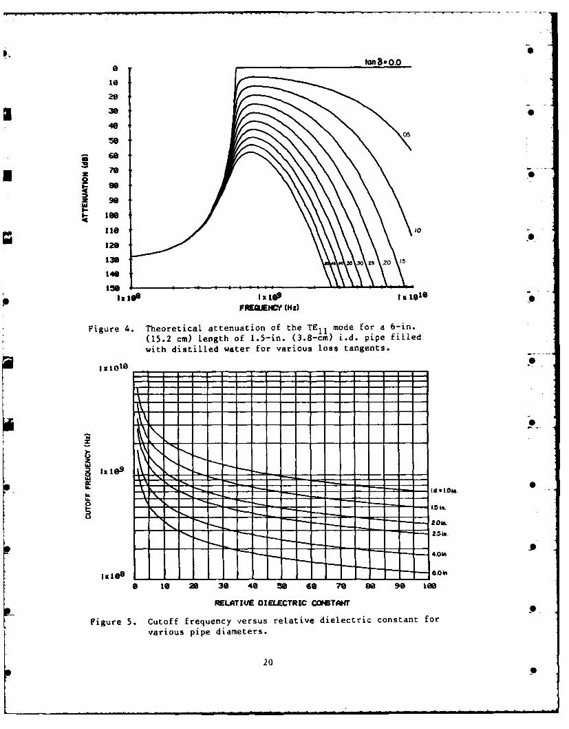
4 Theoretical Attenuation of the TE1 Mode for a 6-In. Length of 201.5-In. i.d. Pipe Filled With Distilled Water for VariousLoss Tangents

5 Cutoff Frequency Versus Relative Dielectric Constant for 20Various Pipe Diameters

6 Theoretical Attenuation of a 6-In. Air-Filled Pipe (c = 1) 21for Various Inside Diameters r

7 Theoretical Attenuation of a 6-In. Pipe Filled With Aviation 21Gasoline (100 octane) (c 2) for Various Inside Diameters

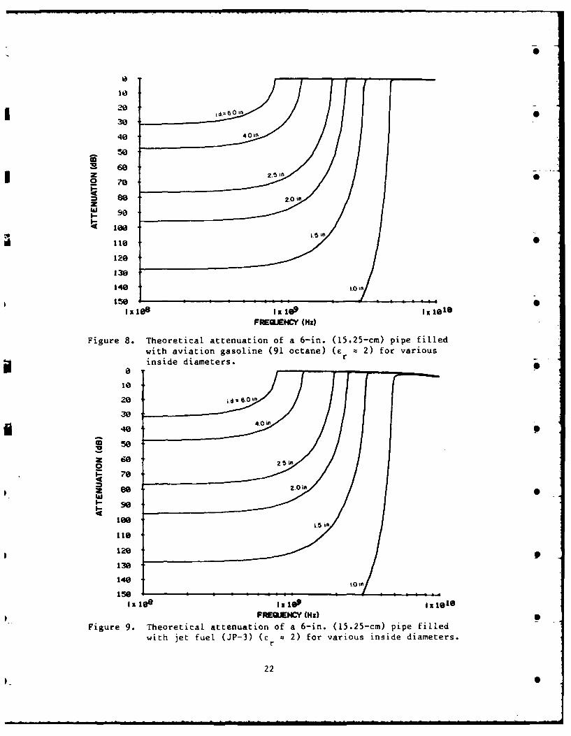
8 Theoretical Attenuation of a 6-In. Pipe Filled With Aviation 22Gasoline (91 Octane) (e - 2) for Various Inside Diameters

r

9 Theoretical Attenuation of a 6-In. Pipe Filled With Jet Fuel 22(JP-3) ( 2) for Various Inside Diameters

10 Theoretical Attenuation of a 6-In. Pipe Filled With Carbon 23Tetrachloride (c = 2) for Various Inside Diameters

r

11 Theoretical Attenuation of a 6-In. Pipe Filled With Cable 23Oil (E 2) for Various Inside Diameters Sr -

12 Theoretical Attenuation of a 6-In. Pipe Filled With Methanol 24(e = 24) for Various Inside Diameters

r

13 Theoretical Attenuation of a 6-In. Pipe Filled With Ethylene 24Gylcol (c r 25) for Various Inside Diameters 0

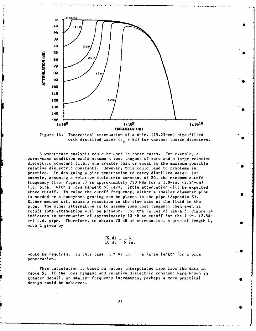
14 Theoretical Attenuation of a 6-In. Pipe Filled With Distilled 25Water (c z 63) for Various Inside Diameters

r

B1 Transmitting and Receiving Antennas 32

B2 Experimental Setup for Reference Measurements 34

B3 Experimental Setup for Waveguide Measurements 34

Cl Program Pipe 1A 38

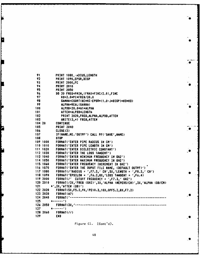
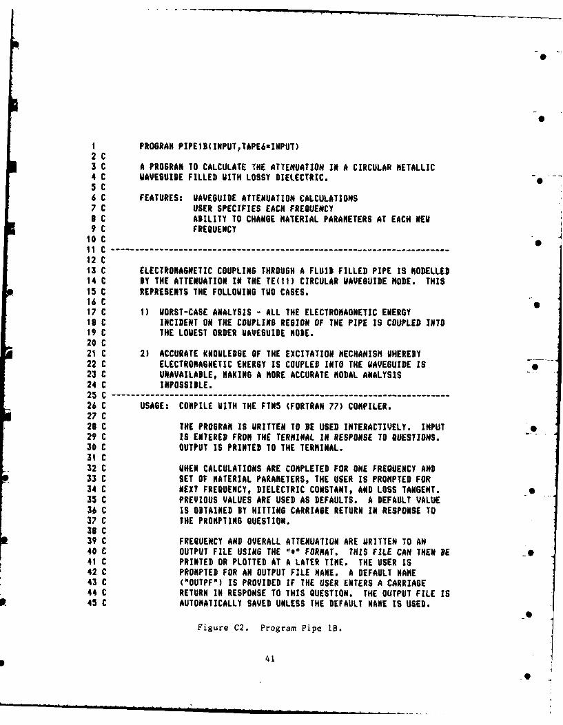
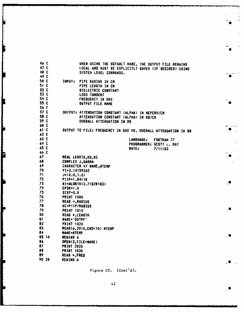
C2 Program Pipe lB 41

6_e

FIGURES (Cont'd)

Number Page .

C3 Sample Run of Program Pipe IA for Distilled Water 46

C4 Sample Run of Program Pipe 1B for Distilled Water 47

El Diagram of the Honeycomb Grating Used in Calculating the 56 -

Attenuations in Tables El, E2, E3, and E4

FL TEM Wave Propagation Through a Multilayered Dielectric Region 59

0

7

THE EFFECT OF FLUIDS ON WAVECUIDES BELOW CUTOFFPENETRATIONS AS RELATED TO ELECTROMAGNETICSHIELDING EFFECTIVENESS

1 INTRODUCTION

Background

It is common practice in electromagnetic pulse (EMP) and electromagneticinterference (EMI) hardened facilities that house sensitive electronic

equipment to enclose part or all of the facility in a metallic electromagneticshield. This shield must have openings for personnel and equipment access,electric power entry, communications and control cooling, heating, 0

ventilating, air-conditioning (HVAC), and entry of various fluids such aswater and refrigerants. Technology for the design of these penetrations is,in general, highly advanced and is discussed in numerous technical manuals anddesign handbooks.

When it is required to bring fluids through a shield, it must be done in •

a manner which does not compromise the shield. One approach is to use acompletely closed metallic piping or conduit system into which compromisingelectromagnetic energy cannot enter. The metallic pipe or conduit typicallyis welded or otherwise electrically connected around its periphery to the

shield at the point of entry.

Another approach is to use a short length of metallic pipe to penetratethe shield. This length of pipe acts as a waveguide below cutoff, blockingunwanted electromagnetic energy. (A waveguide passes only those frequencies

above a particular "cutoff" frequency.) This technique is used to isolate thepipe ground from the shield ground without compromising the shield. It alsopermits the connection of nonmetallic pipes to the shield without a loss inshielding.

A honeycomb grating is an extension of the waveguide below cutoffconcept. A honeycomb grating is made of many tubular cells with hexagonalcross sections. Each cell acts as a waveguide below cutoff.

Typically, when designing shield penetrations, the pipes are assumed tobe air-filled. In practice, however, it is often necessary to bring fluidsother than air through the pipes. Examples are tapwater, distilled water,fuel, refrigerants, fire extinguishing fluids, and freeze prevention fluids.These fluids may have relative dielectric constants and dissipation factors -

1DASA EMP Handbook, DASA 2114-1 (Defense Atomic Support Agency [DASAI Infor-mation and Analysis Center, September 1968); DNA EMP Awareness Course Notes,Third Ed, DNA 2772T (Defense Nuclear Agency, October 1977); EMP EngineeringPractices Handbook, NATO file No. 1460-2 (October 1977); Nuclear Electro-magnetic Pulse (NEMP) Protection, TM 5-855-5 (Headquarters, Department of theArmy, February 1974).

9

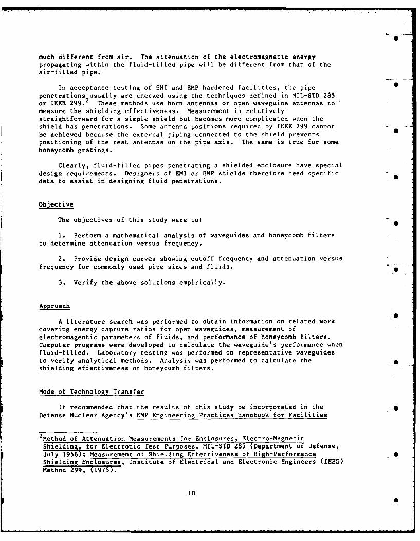
much different from air. The attenuation of the electromagnetic energypropagating within the fluid-tilled pipe will be different from that of the

air-fiLled pipe.

In acceptance testing of EMI and EMP hardened facilities, the pipe 0penetrations usually are checked using the techniques defined in MIL-STD 285

or IEEE 299.2 These methods use horn antennas or open waveguide antennas tomeasure the shielding effectiveness. Measurement is relativelystraightforward for a simple shield but becomes more complicated when theshield has penetrations. Some antenna positions required by IEEE 299 cannotbe achieved because the external piping connected to the shield preventspositioning of the test antennas on the pipe axis. The same is true for somehoneycomb gratings.

Clearly, fluid-filled pipes penetrating a shielded enclosure have specialdesign requirements. Designers of EMI or EMP shields therefore need specific 0data to assist in designing fluid penetrations.

Objective

The objectives of this study were to:

1. Perform a mathematical analysis of waveguides and honeycomb filters

to determine attenuation versus frequency.

2. Provide design curves showing cutoff frequency and attenuation versus

frequency for commonly used pipe sizes and fluids.

3. Verify the above solutions empirically.

Approach

A literature search was performed to obtain information on related work

covering energy capture ratios for open waveguides, measurement of

electromagentic parameters of fluids, and performance of honeycomb filters.Computer programs were developed to calculate the waveguide's performance whenfluid-filled. Laboratory testing was performed on representative waveguidesto verify analytical methods. Analysis was performed to calculate the 0

shielding effectiveness of honeycomb filters.

Mode of Technology Transfer

It recommended that the results of this study be incorporated in the

Defense Nuclear Agency's EMP Engineering Practices Handbook for Facilities

2Method of Attenuation Measurements for Enclosures, Electro-Magnetic

Shielding, for Electronic Test Purposes, MIL-STD 285 (Department of Defense,July 1956); Measurement of Shielding Effectiveness of High-Performance S

Shielding Enclosures, Institute of Electrical and Electronic Engineers (IEEE)

Method 299, (1975).

10

. . . . . . . . . . . .. . . . . . . . ! . . . . . . . . . . . . . . . . . . . . . .. . .. . . . . .

which is in preparation. it is also recommended that these results be

included in Army Technical Manual (TM) 5-855-5, Nuclear Electromagnetic Pulse

(NEMP) Protection.

L0

O

itS

.. . . .. ... . .... . . . . . ... . I| | | " ! ... .. .. .. . . . . . . . . ..

2 THEORY AND PROCEDURE

Introduction

This chapter describes the analysis of a dielectric loaded waveguide.Specifically, the modes excited in a waveguide by an incident plane wave andthe accuracy of shielding tests such as IEEE 299 and MIL-STD-285 areaddressed. An experimental verification for the theoretical analysis of theloaded waveguide is included.

A waveguide is a hollow metallic pipe (usually circular or rectangular)through which electromagnetic energy propagates. The most important waveguideparameter is its cutoff frequency, that is, the frequency at which thewaveguide starts dissipating the electromagnetic energy instead of propagatingit. Frequencies above cutoff are passed through the waveguide with noattenuation. Frequencies below cutoff are heavily attenuated within thewaveguide.

The waveguide cutoff frequency is a function of the waveguide crosssectional area and the contents of the waveguide. The larger the crosssectional area, the lower the cutoff frequency. Generally, any fluid in thewaveguide besides air will have a lower cutoff frequency than the air-filled

waveguide.

A waveguide below cutoff penetration of a shield consists of a length ofmetal pipe passing through the shield. Where the pipe penetrates the shield,the pipe periphery is electrically connected to the shield.

Waveguide below cutoff penetrations are used in plastic pipe systems toblock unwanted electromagnetic energy. They are also used to eliminate groundloops.

In most shielded facilities, numerous piping and conduit penetrationswill be required, possibly at widely spaced points. The piping and conduitoutside the shield act as electromagnetic energy collectors. Many of thesepipes and conduits pass underground and thus are earth-grounded. The use ofmany earth-grounded piping systems with shield penetrations createselectromagnetic energy collecting ground loops. These ground loops are notconsistent with optimized grounding system philosophy, so it may be necessaryto electrically disconnect the piping system from the shield. This iscommonly done by inserting nonmetallic pipe sections near the shield, thenpenetrating the shield with a waveguide below cutoff piping section.

Circular Waveguide Theory

Figure 1 shows the basic geometry of a pipe penetrating a shieldedenclosure. The pipe has inside diameter d and length L. It contains a fluidwith relative dielectric constant E and _oss tangent tan S. A plane wave is

incident from the left, propagating ralong the z-axis.

12

. . . . . . . . . . .. . . I I I I H - " " I i i I l | i l I . . . . I . . . . . . . . .

dS

L

Figure 1. Geometry of pipe penetrating a shield.

A rigorous analysis of the electromagnetic energy coupled into the pipeand then into the enclosure is difficult. Because the relative dielectricconstants, loss tangents, frequencies, and pipe dimensions vary widely,several types of analysis are required. Most importantly, a rigorousmultimodal examination of the problem would require precise knowledge of the

excitation mechanism.

The forms of excitation found in practice are likely to vary widely andwould most certainly differ from the basic geometry just described. Becauseof this difference, an approximate transverse electric and magnetic fields(TEM)-waveguide analysis is used to obtain the shielding effectiveness of thepipe alone. Inclusion of a particular excitation mechanism would increase

shielding effectiveness because the coupling of the incident wave to the pipe

is imperfect.

Appendix A presenta the basic equations for the analysis of electro-magnetic wave propagation through a circular waveguide (pipe).

Modes Excited in a Circular Waveguide

Typically, most of the energy in a waveguide is carried in the first fewpropagating modes. This was observed during the tests conducted for thisreport.

Figure 2 is a plot of energy propagation through a 1.5-in. (3.81-cm)

inside diameter (i.d.) pipe as a function of frequency. The pipe was excitedby a plane wave as shown in Figure 1. The vertical scale represents theattenuation resulting from the pipe relative to free space.

13

I-'10-

20-

30-

~40-zIQ50I

0-

7160 -

80 I I90- I

100 -

110i I iS

1 2 3 4 15 7 8 9TElI TMOI

FREQUENCY(GHz)

Figure 2. Transmission through an air-filled 1.5-in. (3.8-cm)

i.d. pipe.

For an air-filled pipe, the two lowest modes are the TE1 l and TMO1 modes

with cutoff frequencies of 4.7 and 6.14 GHz, respectively. Pigure 2 clearlyshows that the TEll must be present. Also, there is no significant increasein the power transfierred above the TMoI cutoff frequency, indicating that most

of the energy is coupled into the TE1 1 mode.

Computer Model of a Circular Waveguide

Appendix C contains listings and descriptions of two FORTRAN V programs,Pipe 1A and Pipe lB (Figures Cl and C2), that compute the theoretical

attenuation resulting from a Length of pipe. Both programs are designed foruse on an interactive computer system. The frequency and corresponding

attenuation are written into a named file for storage. The user is questioned

for the problem parameters. 9

Program Pipe 1A computes the attenuation over a band of frequencies. The

relative dielectric constant and Loss tangent are assumed to be constant over

this band. The variables to be entered are: pipe inside radius, pipe length,

relative dielectric constant, loss tangent, minimum frequency in band, maximumfrequency in band, the frequency increment to be used within the band, and the

name of the output file in which the results are to be stored.

Program Pipe IB computes the attenuation for a particular frequency. The

program is cyclical so the attenuation at any number of frequencies may be

computed. However, the pipe inside radius and pipe length are entered onlyonce. The parameters to be entered are: pipe inside radius, pipe length, thename of the output file in which the results are to be stored, frequency 1,

14

~0

relative dielectric constant 1, loss tangent 1, frequency 2, relative

dielectric constant 2, loss tangent 2, frequency 3,.

Experimental Verification 0

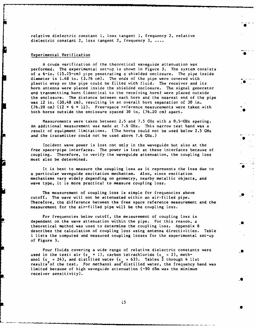
A crude verification of the theoretical waveguide attenuation wasperformed. The experimental set-up is shown in Figure 3. The system consistsof a 6-in. (15.25-cm) pipe penetrating a shielded enclosure. The pipe insidediameter is 1.48 in. (3.76 cm). The ends of the pipe were covered withplastic wrap so the pipe could be filled with fluid. The receiver and its .horn antenna were placed inside the shielded enclosure. The signal generator

and transmitting horn (identical to the receiving horn) were placed outsidethe enclosure. The distance between each horn and the nearest end of the pipewas 12 in. (30.48 cm), resulting in an overall horn separation of 30 in.(76.20 cm) (12 + 6 + 12). Free-space reference measurements were taken withboth horns outside the enclosure spaced 30 in. (76.20 cm) apart.

Measurements were taken between 2.5 and 7.5 GHz with a 0.5-GHz spacing.

An additional measurement was made at 7.6 GHz. This narrow test band was aresult of equipment limitations. (The horns could not be used below 2.5 GHzand the transmitter could not be used above 7.6 GHz.)

Incident wave power is lost not only in the waveguide but also at thefree space-pipe interfaces. The power is lost at these interfaces because of

coupling. Therefore, to verify the waveguide attenuation, the coupling loss

must also be determined.

It is best to measure the coupling loss as it represents the loss due toa particular waveguide excitation mechanism. Also, since excitationmechanisms vary widely depending on geometry, nearby metallic objects, andwave type, it is more practical to measure coupling loss.

The measurement of coupling loss is simple for frequencies abovecutoff. The wave will not be attenuated within an air-filled pipe.Therefore, the difference between the free space reference measurement and themeasurement for the air-filled pipe will be the coupling loss.

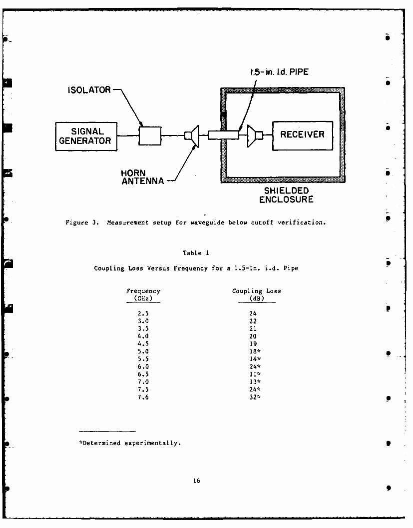
For frequencies below cutoff, the measurement of coupling loss isdependent on the wave attenuation within the pipe. For this reason, atheoretical method was used to determine the coupling loss. Appendix Bdescribes the calculation of coupling loss using antenna directivities. Table1 lists the computed and measured coupling losses for the experimental set-upof Figure 3.

Four fluids covering a wide range of relative dielectric constants wereused in the test: air (e = 1), carbon tetrachloride (e 2 2), meth-anol (c z 24), and distilled water ( = 63). Tables through 4 listresults rof the test. For methanol andrdistilled water, the frequency band waslimited because of high waveguide attenuation (-90 dBm was the minimum

receiver sensitivity).

15

1.5- in. I.d. PIPE

ISOLATOR

SIGN L REEIVE

GENERATOR

HORNANTENNA /. .~.

SHIELDEDENCLOSURE

Figure 3. Measurement setup for vaveguide below cutoff verification.

Table 1

Coupling Loss Versus Frequency for a 1.5-In. i.d. Pipe

Frequency Coupling Loss(0Hz) (dB)

2.5 243.0 223.5 214.0 204.5 195.0 18*5.5 14*6.0 24*6.5 11*7.0 13*7.5 24*7.6 32*

*Determined experimentally.

16

tS

Table 2

Transmission Loss Through 1.5-In. i.d. Pipe FilledWith Carbon Tetrachloride

Theoretical

Free-space attenuation Coupling

Frequency reference in pipe loss Computed Actual

(CHz) (dB) (dB) (dB) measurement measurement

2.5 -5 81 24 -110 -793.0 13 44 22 -53 -373.5 11 0 21 -10 - 8

4.0 7 0 20 -13 - 84.5 7 0 19 -12 - 8

5.0 7 0 18 -11 -11

5.5 2 0 14 -12 -12

6.0 12 0 24 -12 -13

6.5 -7 0 11 -18 -19

7.0 -19 0 13 -32 -33

7.5 -15 0 24 -39 -38

7.6 -11 0 32 -43 -41

Table 3

Transmission Loss Through 1.5-In. i.d. Pipe Filled With Methanol

Reference 0

Frequency free Coupling Theoretical Computed Actual

(GHz) space loss attenuation measurement measurement

4.0 7 20 65 -78 -83

4.5 7 19 67 -79 -87

5.0 7 18 65 -76 -81 0

Table 4

Transmission Loss Through 1.5-In. i.d. Pipe Filled With Distilled Water

Reference 0

Frequency free Coupling Theoretical Computed Actual(GHz) space loss attenuation measurement measurement

2.5 -5 24 47 -76 -74

3.0 13 22 58 -67 -72

3.5 11 21 68 -78 -79

4.0 7 20 67 -80 -77

4.5 7 19 66 -78 -845.0 7 18 59 -70 -82

5.5 2 14 54 -66 -85

6.0 12 24 53 -65 -79

6.5 -7 11 52 -70 -84 e

17

. . .. . . . .. . . . , = ,, , i i= . .... . . .

The theoretical attenuation in the pipe was found using program PipelB. Because of the lack of published data on relative dielectric constantsand loss tangents, these parameters were measured using a dielectric slabtechnique. Appendix D describes this technique and lists the values of the -relative dielectric constants and loss tangents used in computing thewaveguide attenuation.

The predicted measurement is equal to the free-space reference minus thesum of the coupling loss and theoretical waveguide attenuation (i.e., column 5= column 2 - (column 3 + column 41 in Tables 2 through 4). The last column --

contains the actual measurement.

For carbon tetrachloride, the agreement between predicted and actualmeasurements is fairly good above cutoff. Below cutoff, the error isextremely large. No reason for this disagreement is known.

For methanol and distilled water, the actual measurement is consistentlyless than the predicted measurement (except in two cases). This can beexplained by the reflection and refraction of the electromagnetic wave at theair-fluid interface. Electromagnetic waves undergo reflection and refractionat interfaces where the relative dielectric constants change. The reflectioncoefficient, R, is given by: 0

R 2 [Eq II

where .is the relative dielectric constant of the first medium and r2 is the1 2

relative dielectric constant of the second medium. Therefore, the greater themismatch of relative dielectric constants, the greater the reflection at theinterface. This means there will be an additional power loss due toreflection and thus, a lower value of transmitted power.

Shielding Tests for Circular Waveguides

It is important to consider the accuracy of standard shielded enclosuretest procedures in measuring the shielding effectiveness of enclosures withpipe penetrations. The cutoff frequency of a pipe is inversely proportionalto the pipe radius and to the square root of the relative dielectric constantof the fluid in the pipe (i.e., as r or VE increases, the cutoff frequencydecreases). Neither MIL-STD-285 nor IEEE 599 make any statement about thecontents of the penetrating pipe while it is being tested. Since any fluidbesides air in the pipe will lower the cutoff frequency, it is important tohave the pipe filled as it would be under normal use. Since the greatestamount of electromagnetic energy is coupled into the pipe when the plane wave pis axially incident, the shielding effectiveness measurements should be takenwith the transmitting and receiving antennas positioned along the pipe axis.

1

18

3 RESULTS

This chapter presents a series of graphs produced from FORTRAN Program 0Pipe lB to be used in designing pipe penetrations for shielded enclosures.Before presenting these graphs, a few comments will be made about the effectof material parameters on waveguide attenuation and cutoff frequency.

Effect of Material Parameters on Attenuation

The loss tangent of the dielectric affects attenuation whereas the

relative dielectric constant affects cutoff frequency. By definition, thecutoff frequ.ncy affects the attenuation. Figure 4 gives the attenuation ofthe lowest order mode (TE1 A) of a 6-in. (15.24-cm) length of 1.475-in. (3.746-cm) i.d. pipe for distille water at various loss tangents. The loss tangentand the relative dielectric constant are held constant throughout the ,frequency band. The value of the relative dielectric constant is 68.11. Theloss tangent is stepped from 0.0 to 0.50 in 0.05 increments. The major effectof the loss tangent is to increase the attenuation. Note that a small changein the loss tangent can change the attenuation considerably, especially atfrequencies well above cutoff.

Curves showing the change in cutoff frequency of the lowest order modewith relative dielectric constant are given in Figure 5. The curves represent

pipe i.d. of 1.0 in. (2.54 cm), 1.5 in. (3.81 cm), 2.0 in. (5.08 cm), 2.5 in.(6.35 cm), 4.0 in. (10.16 cm), and 6.0 in. (15.24 cm). The relativedielectric constants range from I to 100. Note the steepness of each curvefor low relative dielectric constants. This is caused by the inverse squareroot dependence of cutoff frequency on the relative dielectric constant.

Design Curves

Figures 6 through 14 give the attenuation of the lowest order mode (TE11 )in a 6-in. (15.24-cm) length of pipe for various fluids

and pipe i.d.

values. Each figure consists of six curves corresponding to i.d. values of

1.0 in. (2.54 cm), 1.5 in. (3.81 cm), 2.0 in. (5.08), 2.5 in. (6.35 cm), 4.0in. (10.16 cm), and 6.0 in. (15.24 cm). 3The relative dielectric constants and

loss tangents were taken from von Hippel and are summarized in Table 5. Forintermediate frequencies, a linear interpolation was performed on the givenvalues. Because attenuation is directly proportional to length, to find the

attenuation from a pipe of length L, the attenuation should be multiplied byL/6 (L in in.).

A few liquids have large changes in relative dielectric constant and losstangent over the 100-MHz to 10-GHz range (e.g., methanol, ethylene glycol, andwater). This might present problems in determining the optimal pipe size,especially since a small change in loss tangent can result in a large changein attenuation (see Figure 4).

3A. R. von Hippel, Dielectric Materials and Applications (Technology Press of

the Massachusetts Institute for Technology, 1954).

19

* 40

585

9 9

14

116

158 ~FR.S.EtCY (HO)11 1

Figure 4. Theoretical attenuation of the TE 1 , mode for a 6-in.(15.2 cm) length of 1.5-in. (3.8-cm) i.d. pipe filledwith distill1ed water for various loss tangents.

z

00

toI 28 30 48 55 so 78 s8 98 too

RELAT1IUE DIELECTRIC CONSTANT

Figure 5. Cutoff frequency versus relative dielectric constant for

various pipe diameters.

20

600

lie

130

140

650

3- 0

40

740

1B8

130

140

t5e60191 0 1II

FRMEC (N

1121

300

60

0 78

W 98

1.5 1P

l1e

120

130

1408.0i

158 0

F~REQENCY (Hz)

Figure 8. Theoretical attenuation of a 6-in. (15.25-cm) pipe filledwith aviation gasoline (91 octane) (c r 2) for various

j inside diameters.r

30

0S 78

lie

138

1408.0i

158

FREQUENCY (Hz)Figure 9. Theoretical attenuation of a 6-in. (15.25-cm) pipe filled

with jet fuel (JP-3) (c r 2) for various inside diameters.

22

20

'340n6n40

50

0 6020 i

z96

126

138

I le18x10 isle,@FREGLENGY (Hz)

Figure 10. Theoretical attenuation of a 6-in. (15.25-cm) pipe filled

with carbon tetrachloride (E r 2) for various inside

A diameters. 0

30 4i

460

50

20i

I- 90

126

136

146 oi

156

FREVIENCY (Hz)

F~igure 11. Theoretical attenuation of a 6-in. (15.25-cm) pipe filled

with cable oil (c 2) for various inside diameters.r

23

100

40

56.

* ~ 60

07

~- 90 15i

IS-

lie

128

130

146

156 18

FREQUENCY (Hz)

Figure 12. Theoretical attenuation of a 6-in. (15.25-cm) pipe filledwith methanol (c u24) for various inside diameters.

r

10

20

40 40

50

z 60

00

le

120

130 10i

140

156

LD FR9EUENC WS)Figure 13. Theoretical attenuation of a 6-in. (15.25-cm) pipe filled

with ethylene glycol (c 25) for various inside diameters.

24

i d - 6 0 in]

20i

30

70

Sso90

1170

I-4

110

126 a

140

156IslsI x I9 9 I1 1

FREQLEHCY (Hz)

Figure 14. Theoretical attenuation of a 6-in. (15.25-cm) pipe.filledwith distilled water (e = 63) for various inside diameters. 0

r

A worst-case analysis could be used in these cases. For example, aworst-case condition could assume a loss tangent of zero and a large relativedielectric constant (i.e., one greater than or equal to the maximum possiblerelative dielectric constant). H6wever, this could lead to problems in 0practice. In designing a pipe penetration to carry distilled water, forexample, assuming a relative dielectric constant of 80, the maximum cutofffrequency (from Figure 5) is approximately 750 MHz for a 1.0-in. (2.54-cm)i.d. pipe. With a loss tangent of zero, little attenuation will be expected

above cutoff. To raise the cutoff frequency, either a smaller diameter pipeis needed or a honeycomb grating can be placed in the pipe (Appendix E).Either method will cause a reduction in the flow rate of the fluid in thepipe. The other alternative is to assume some loss tangent; then even atcutoff some attenuation will be present. For the values of Table 5, Figure 14indicates an attenuation of approximately 10 dB at cutoff for the I-in. (2.54-cm) i.d. pipe. Therefore, to obtain 70 dB of attenuation, a pipe of length L,with L given by

70 dB L10 dB 6 in.

would be required. In this case, L = 42 in. -- a large length for a pipe

penetration.

This calculation is based on values interpolated from from the data inTable 5. If the loss tangent and relative dielectric constant were known ingreater detail, at smaller frequency increments, perhaps a more practical

design could be achieved.

25

Table 5 0

Relative Dielectric Constants and Loss Tangents for

Various Materials*

Frequency Relative dielectric constant Loss tangent(MHz) (C ) (tan 4)r

Air

100 1 01000 1 0

10000 1 0

Aviation gasoline - iOO Octane

300 1.94 .000083000 1.92 .0014

Aviation gasoline - 91 Octane

300 1.95 .000043000 1.94 .0015

Jet fuel - JP-3

300 2.08 .00073000 2.04 .0055

Carbon tetrachloride

100 2.17 <.0002300 2.17 <.0001

3000 2.17 .000410000 2.17 .0016

Cable oil - Type 5314 (CE)

300 2.24 .00393000 2.22 .0018

10000 2.22 .0022

Methanol at 25°C

100 31.0 .038300 30.9 .080 0

3000 23.9 .64010000 8.9 .810

Ethlyene Glycol at 2SC

100 41 .045300 39 .160 9

3000 12 1.00010000 7 .780

Distilled water at 25°C

300 77.5 .0163000 76.7 .157

10000 55.0 .540 0

*From A. R. von Hippel. These date were used to plot the curves shown in

Figures 6 through 14.

2

26

- . .= = ., .A . - •

4 CONCLUSIONS

This report has addressed the electromagnetic shielding effectiveness of

waveguide sections (pipes) filled with fluids. An analytical method for 0

determining the coupling between horn antennas when used to measure shieldingeffectiveness of shields with pipe penetrations has been presented.Analytical methods including computer codes for calculating attenuation versus

frequency within the pipe sections have been developed and verifiedexperimentally. From these analytical methods, design curves have beenproduced for commonly used pipe sizes and fluids. Similarly, analytical 0

methods have been developed for honeycomb filters and calculations have been

made to show shielding effectiveness of this filter versus frequency. Results

show that:

1. For fluids with relatively high dielectric constants and low losstangents, currently used designs can compromise the effectiveness of the 0

shield.

2. A honeycomb grating can have its shielding effectiveness

substantially reduced if filled with distilled water instead of air.

A problem encountered in this study is that published data on the 0

relative dielectric constant and loss tangent are incomplete for most fluids

of interest.

27

APPENDIX A:

WAVE PROPAGATION IN CIRCULAR METALLIC WAVEGUIDES

The analysis of circular metallic waveguides can be found in manystandard electromagnetic textbooks. Significant results are summarized here.

A circular metallic pipe supports both TE and TM waveguide modes. Thepropagation constants of these modes are given by:

c- f( n M) 2

8n,m v'-r ko ( f 2 [Eq All

where e = relative dielectric constant of the medium filling the waveguider

ko = free space wave number

fc(n,m) = cutoff frequency of the TEn,m or TMn, mode

f = frequency of operation. 0

Equation Al is valid for f > fc(n,m)" For TE modes, the cutoff frequency isgiven by:

f - c°n 2

c(n,m) 27 a /[Eq A2r

where a = radius of the waveguide

c = speed of light in free space

= the mth root of J ', the first derivative of the nthorder Bessel function

Similarly, for TM modes:

f L n m c 0 A31c(n,m) 2,i a [Eq A3]

r

where pn, m the mth root of Jn' the nth order Bessel function.

The on and p'nmvalues can be found in standard mathematical tables.5

Tables Al afi A2 list values of p for m = 1, 2, 3 and n = 0, 1, 2, 3.n,m

4 S. Ramo, J. Whinnery, and T. Van Duzer, Field and Waves in Communication 9Electronics (John Wiley and Sons, Inc., 1965); R. E. Collin, Field Theory ofGuided Waves (McGraw-Hill, Co., 1960).

5M. Abramovitz and I. Stegun, Handbook of Mathematical Functions (Dover Press,1970).

2 9~28

Table Al

Roots of J', Derivative of the nth Order Bessel Functionn

nm 0 1 2 3

1 3.832 1.841 3.054 4.2012 7.016 5.331 6.706 8.015

3 10.173 8.536 9.969 11.346

Table A2

Roots of Jn, nth Order Bessel Function

nm 0 1 2 3

1 2.405 3.832 5.136 6.3802 5.520 7.016 8.417 9.761

3 8.654 10.173 11.620 13.015

For fc < i c(n,), the (n,m) waveguide mode is "cutoff." The attenuationconstant is given Y:

=(n 2. [Eq A4n,m r o f .A

where c r, ko' fc(n,m) and f are as defined in Equation Al.

These results, typically derived for the case in which the waveguide isfilled with a lossless medium, are readily extended to the lossy case byallowing r to be complex. Denoting the complex dielectric constant by r*rS

E * - i a [Eq ASr r WE

where E = real relative dielectric constantr

o = conductivity of the medium

0 = free-space permittivity0

w = 21f.

29

. . . . . . . . ... . . . A . . .. . . . . . . .... . . . . . .

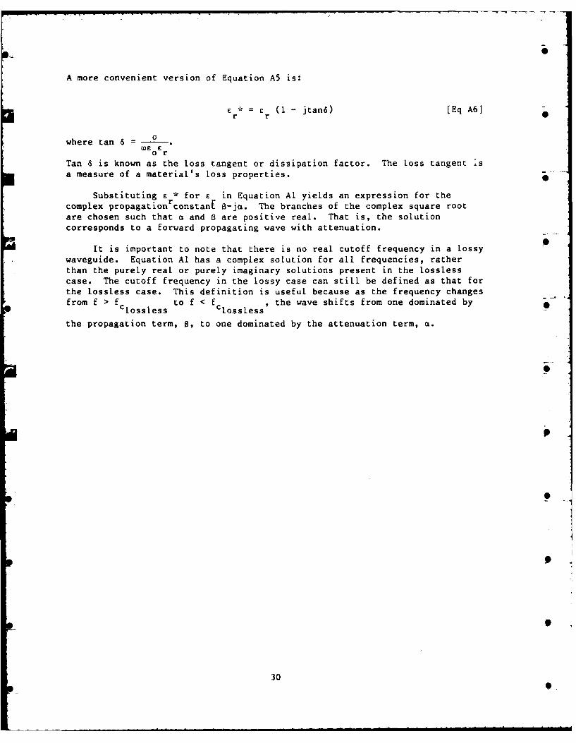
A more convenient version of Equation A5 is:

C * = r (1 - jtan6) [Eq A6]r r

0

where tan 6-WC C

orTan 6 is known as the loss tangent or dissipation factor. The loss tangent isa measure of a material's loss properties.

Substituting e * for c in Equation Al yields an expression for thecomplex propagation constanl B-ja. The branches of the complex square rootare chosen such that a and B are positive real. That is, the solutioncorresponds to a forward propagating wave with attenuation.

0It is important to note that there is no real cutoff frequency in a lossy

waveguide. Equation Al has a complex solution for all frequencies, ratherthan the purely real or purely imaginary solutions present in the losslesscase. The cutoff frequency in the lossy case can still be defined as that forthe lossless case. This definition is useful because as the frequency changesfrom f > f to f < f , the wave shifts from one dominated by 0

clossless Clossless

the propagation term, 8, to one dominated by the attenuation term, a.

3

p

30p e

APPENDIX B:

COUPLING OF ELECTROMAGNETIC WAVES TO A CIRCULAR WAVEGUIDE

When an electromagnetic wave is incident on the open end of a circular

waveguide, some of the wave's energy will be coupled into the waveguide.

Analysis of the coupling factor is complicated by diffraction of the incident

wave by the waveguide end. Pearson has determined theoretically the fieldswithin the waveguide for a plane harmonic electromagnetic wave ingident on a - -.

semi-infinite open-ended perfectly conducting circular waveguide. This 6

problem has been addressed experimentally by Southworth and King.7

Experiments were done to determine the directive properties of metal pipes and

horns when used as electromagnetic wave receivers. This appendix presents hhe

basic textbook approach to power transfer between transmitter and receiver.

Two important antenna parameters are directivity and effective 0

aperture. The directivity of an antenna is a measure of the relativeconcentration of radiated or received power in different directions. It isdependent on antenna type and size.

Effective aperture is defined as the ratio Df the power in the antennaterminating impedance to the power density of the incident wave. Under

conditions of maximum power transfer and zero antenna losses, the effective

anerture is a maximum. Maximum effective aperture is related to directivity

through the expression:

D = 4A [Eq B1I

em

where D is the directivity, Aem is the maximum effective aperature and X is

the wavelength.

Consider a transmitting antenna with directivity DT and a receiving -0

antenna with maximum effective aperture AeR (Figure Bi). The antennas are

separated by a distance d. The received power, PR' is given by:

R P = D[ AR [Eq B2] 0

6 J. D. Pearson, "The Diffraction of Electro-Magnetic Waves by a Semi-Infinite

Circular Wave Guide," Proceedings of the Cambridge Philosophical Society,Vol 49, Part 4 (1953), pp 659-667.

7G. C. Southworth, and A. P. King, "Metal Horns as Directive Receivers of

Ultra-Short Waves," Proceedings of the I.R.E., Vol 27 (February 1939), -0

8pp 95-102.8 D. Kraus, Antennas (McGraw-Hill, Co., 1950); R. E. Collin and F. J.Zucker, Antenna Theory, Part I (McGraw-Hill, 1969).

31

rdd

Figure Bi. Transmitting and receiving antennas.

where PT is the transmitted power. This formula assumes a lossless medium andno polarization mismatch. Using Equation Bi, Equation B2 can be expressed interms of the directivity of the receiving antenna, DR:

PX 'dD D T[Eq B31

Therefore, the power transfer ratio between two antennas is:

P R2

-= D DR 4 [Eq B4]PT T RL4Tdj

Equation B4 is a far-field relation and, therefore, will not be valid if d issmall compared to the size of the antenna. The error is small if:

d > 22[Eq B51

where I is the maximum linear dimension of either antenna. p

The directivity of a horn antenna with a large aperture can be written interms of the maximum effective aperture. Thus, from Equation Bl:

D =y4 AEX AHk [Eq B6]

32

A

where A = aperture length in free-space wavelengths in k plane

AHX = aperture length in free-space waveLengths in H plane

y = ratio of mAximum effective aperture to physical aperture. -

An optimum horn has a value of y z 0.6. Thus, Equation B6 becomes:

D = 7.5 AEX AHk [Eq B7]

The horns used in the tests conducted for this report have an aperture

size of 5.85 in. (14.86 cm) (E-plane) by 7.92 in. (20.12 cm) (H-plane). So,

14.86 cm

A = 20.12 cm [Eq B8]HX X

Therefore, the directivity of the horn antennas, DH, is given by

DZ 7.5 14.86 20.12]= 2242 (EqB91i "xJ 2

where X is measured in cm.

The open-ended waveguide can be considered as an antenna. The

directivity of an open-ended circular waveguide is given by

2DpZ 10.5 wL2 [Eq BI1

where r is the radius of the waveguide. The pipes (circular waveguides) usedin the tests have radii of 0.738 in. (1.874 cm) and 2.0 in. (5.08 cm). Thus,

D 10.5n (1.874)2 116 [Eq Bil11s 2 (1.[874)] •...

for the small pipe and

D 10.57 (5.08)2 = 851PL x2 x2

for the large pipe. Again, X is measured in cm.

Figures B2 and B3 show the placement of the horn antennas used in thesetests. Figure B2 shows the positioning in free space for the referencemeasurements. The distance d was measured from mouth to mouth. For testingthe waveguide below cutoff theory, the configuration in Figure B3 was used.

33

SHIELDED ROOM

d

TRANSMITTER S

Figure B2. Experimental setup for reference measurements. 0

SHIELDED ENCLOSURE

= . TRANSMITTER "RECEIVER

Figure B3. Experimental setup for waveguide measurements.

34- S

rhe waveguide was 6 in. (15.24 cm) long with a radiuti r, and d' is the

distance trom the horn mouth to the end of the waveguide.

As an example calcuLation for coupling toss, consider a. pLane wave at 2.5

CHz propagating from the transmitting antenna toward the large pipe. Some of 0

the transmitted wave power will be coupled into the pipe and some will be

diffracted, which results in a coupling loss. Some of the wave power that

coupled into the pipe will retransmit at the other end of the pipe. Again,

there will be a coupling loss. Finally, the resultant wave power will be

sampled by the receiving horn.

The coupling loss is one-half the dB difference between horn-to-horn

power transfer and horn-to-pipe-to-horn power transfer. if PH H denotes the

power transfer ratio between the two horns in free space and PH-P-H denotes

the power transfer ratio between the two horns separated by the pipe, then

coupling loss, LC, s:

PH- -pH--

Lc = H-H H-P-H (in dB) [Eq B131

Let the horn-to-horn distance d (Figure B2) be 78 in. (198 cm). Then:

PH-H =P T R

= D D f [j12 [Eq B14]

Using Equation B9:

PH-H = 2 4 fd] [Eq B151

Recalling:

1010

X c 3 - = 12 cm [Eq B16]f 2.5 x 109 9

Thus,

P [1442J 2 4 198) = .00564 [Eq B17]

Expressed in dB:

PH-H = 10 log 10 (.00564) = -22.5 [Eq B18]

35

Let the horn-to-pipe distance d' (Figure B2b) be 36 in. (91.4 cm). Then:

P D D [ 2 [Eq B9H-P L H P 4~

Using Equations B9 and B12:

H-P L _ 2'd

Thus,

w~P - 22421 F5] 12 2 .01 (Eq B211L-PL 144 j 4 ] L (91.4)

Expressed in dB:

PH-PL -20 dB [Eq B22]L

Because of reciprocity:

PH-PL = P-H [Eq B23]

So:

PHPLH = 2 PHPL =-40 dB [Eq B241

Therefore,

-22.5 - (-40) = 8.75 dB [Eq B25]LC = 2

With the transmitter supplying 5 W at 2.5 GHz, a value of +5 dBm was

measured by the receiver for the reference measurement. The waveguide Smeasurement was -10 dBm. This results in a measured coupling loss of:

= +5 - (-10) _ 7.5 dB [Eq B26]

The error in reading the receiver is +1/2 dB, giving a +3/4 dB error inthe measured coupling loss. Greater error probably exists in the referencemeasurement. Because of cable constraints (too short), it was not possible tomove the receiving horn farther than 36 in. (91.4 cm) from the shieldedenclosure. This put the receiving horn in the "standing wave" field betweenthe enclosure and the transmitting horn, resulting in a non-free-field 9measurement for the reference reading.

36

APPENDIX C:

FORTRAN PROGRAMS TO CALCULATE WAVEGUIDE ATTENUATIONRESULTING FROM DIELECTRIC LOADING

Programs Pipe lA and Pipe lB (Figures Cl and C2) calculate the overall

attenuation in dB of an electromagnetic wave propagating through a length ofcircular waveguide (pipe). Program Pipe lA uses one relative dielectric

constant and loss tangent to compute the attenuation for a band offrequencies. Program Pipe lB uses a separate relative dielectric constant andloss tangent for each frequency.

The attenuation factor (in Np/cm) of a circular waveguide is the realpart of the complex propagation constant,

22y = -t w l [Eq Cl]nm

where w = angular frequency (rad/sec)

p= permeability of the material in the waveguide•

e = permittivity of the material in the waveguide, and:

(ha)m nm [Eq C21hnm a .

where a is the pipe radius and (ha) is the mth root of a BesseL function ofonm

the nth order. Values of (ha) for TM modes are given in Appendix A, TableA2; values of (ha)nm for TE modes are given in Table Al.

The cutoff frequency of the (n,m) mode is the frequency for which the

real part of y is zero. Attenuation through the waveguide is a minimum atthe cutoff frequency.

hf _ nm [Eq C3] 0c 2iue'[

Since

c - [Eq C4]

where c is the speed of light in a vacuum,

37

I PROGRAM PIPE1A(INPUT,TAPE6OINPUT)2C3 C A PROGRAM TO CALCULATE THE ATTENUATION IN A CIRCULAR METALLIC4 C UAVE6UIDE FILLED UITH LOSSY DIELECTRIC.5 C6 C FEATURES: UAVEGUIDE ATTENUATION CALCULATIONS7 C CALCULATIONS OVER A FREQUENCY RANGE8C9C ----------------------------------------------------------------0 Cl1 C ELECTROMAGNETIC COUPLING THROUGH A FLUID FILLED PIPE IS MODELLED12 C BY THE ATTENUATION IN THE TEE11) CIRCULAR VAVEGUIDE NODE. THIS13 C REPRESENTS THE FOLLOUING TUO CASES.14 C15 C 1) UORST-CASE ANALYSIS - ALL THE ELECTROMAGNETIC ENERGY16 C INCIDENT ON THE COUPLING REGION OF THE PIPE IS COUPLED INTO17 C THE LOUEST ORDER UAVEGUIDE NODE. 018 C19 C 2) ACCURATE KNOULEDGE OF THE EXCITATION MECHANISM UHEREDY20 C ELECTROMAGNETIC ENERGY IS COUPLED INTO THE UAVEGUIDE IS21 C UNAVAILADLEt MAKING A MORE ACCURATE MODAL ANALYSIS22 C IMPOSSIBLE.23 C ----------------------------------------------------------------------24 C USAGE: COMPILE UITH THE FTN5 (FORTRAN 77) COMPILER.25 C26 C THE PROGRAM IS URITTEN TO DE USED INTERACTIVELY. INPUT27 C IS ENTERED FROM THE TERMINAL IN RESPONSE TO QUESTIONS.28 C OUTPUT IS PRINTED TO THE TERMINAL.29 C S30 C FREQUENCY AND OVERALL ATTENUATION IS ALSO URITTEN TO AN31 C OUTPUT FILE USING THE "*" FORMAT. THIS FILE CAN THEN BE32 C PRINTED OR PLOTTED AT A LATER TIME. THE USER IS33 C PROMPTED FOR AN OUTPUT FILE NAME. A DEFAULT NAME34 C (*OUTPF") IS PROVIDED IF THE USER ENTERS A CARRIAGE35 C RETURN IN RESPONSE TO THIS QUESTION. THE OUTPUT FILE IS36 C AUTOMATICALLY SAVED UNLESS THE DEFAULT NAME IS USED.37 C UNEN USING THE DEFAULT NAME, THE OUTPUT FILE REMAINS38 C LOCAL AND MUST BE EXPLICITLY SAVED (IF DESIRED) USING39 C SYSTEM LEVEL COMMANDS.40 C41 C INPUT: PIPE RADIUS IN CM42 C PIPE LENGTH IN CM43 C DIELECTRIC CONSTANT44 C LOSS TANGENT45 C MINIMUM FREQUENCY IN GHZ

Figure Cl. Program Pipe 1A.

38*1

0

0

46 C MAXIMUM FREQUENCY IN GHZ

47 C FREQUENCY INCREMENT IN GHZ48 C OUTPUT FILE NAME49 C50 C OUTPUT: ATTENUATION CONSTANT (ALPHA) IN NEPERS/CM S

51 C ATTENUATION CONSTANT (ALPHA) IN DD/CM

52 C OVERALL ATTENUATION IN DD

53 C54 C OUTPUT TO FILE: FREQUENCY IN 6HZ VS. OVERALL ATTENUATION IN DD

55 C56 C LANGUAGE: FORTRAN 77

57 C PROGRANNER: SCOTT L. RAY

58 C DATE: 7/11/83

5? C60 COMPLEX GAMMAJ61 REAL LENGTHKOKC62 CHARACTER *7 NAHEtNTEMP S

63 PI*3.1415926564 J=(0.0,1.0)65 P11P=1.8411866 AI=ALOG1O(2.71928193)67 PRINT 100068 READ *tRADIUS

0

69 KCZP11P/RADIUS70 PRINT 101071 READ *,LENGTH72 PRINT 102073 READ *,EPSR74 FC=1.0/(2.0*PI)*(29.997925/SORT(EPSR))*KC75 PRINT 103076 READ *,DISP77 PRINT 104078 READ *,FMIN79 PRINT 105080 READ *,FMAX81 PRINT 1060

92 READ *,FINC83 NAME=OUTPF"84 PRINT 107085 READ(6,203OtEND=1O) NTEMP 0

96 HANEaNTEMP67 10 REVIND 6

so OPEN(3pFILE=NAME)99 PRINT 206090 PRINT 2040

S0

Figure Cl. (Cont'd).

39S0

91 PRINT 1080, ADIUS,LENGTH92 PRINT 1090,EPSR,DISP93 PRINT 2000,FC94 PRINT 201095 PRINT 205096 DO 20 FREO=FHIN,(FMAX.FINC/2.0),FINC97 KO=2.0.PI*FREQ/30.098 GAMNA=CSORT(KC*KC-EPSR*(I.O-J*DISP)*KO*KO)99 ALPHA=REAL(GANNA)

100 ALPDB=20.0*AI*ALPHA a101 ATTEN=ALPDB*LENGTH102 PRINT 2020,FREQALPHAALPDBATTEN103 URITE(3,*) FREQ,ATTEN104 20 CONTINUE105 PRINT 2040 -

106 CLOSE(3)107 IF(NANE.NE.'OUTPF') CALL PF("SAVE',NAME)fo STOP109 1000 FORNAT('ENTER PIPE RADIUS IN CHI)110 1010 FORMAT('ENTER PIPE LENGTH IN CM')111 1020 FORNAT('ENTER DIELECTRIC CONSTANT')112 1030 FORMAT('ENTER THE LOSS TANGENT')113 1040 FORMAT('ENTER MINIMUM FREQUENCY IN 6H2')114 1050 FORNAT('ENTER MAXIMUM FREQUENCY IN 6HZ')115 1060 FORNAT('ENTER FREQUENCY INCREMENT IN GHZ')116 1070 FORMAT('ENTER THE OUPUT FILE NAME, (DEFAULT OUTPF)')117 1080 FORNAT(/'RADIUS = ',F7.3t' Ch',5X,'LENGTH - ",F8.3p' CH')118 1090 FORNAT('EPSILON - ',F6.2,BX,'LOSS TANGENT a 'pF6.4)119 2000 FORMAT(/' CUTOFF FREQUENCY = 'pF7.3,' 6HZ')120 2010 FORMAT(/3X,'FREO (GHZ)',3X,'ALPHA (NEPERS/CN)',3X,'ALPHA (DB/CN)121 *',3X,'ATTEN (DB)')122 2020 FORNAT(SXFS.2p9X,IPEIO.3,1OXOPFS.2,$XFT.2)123 2030 FORMAT(AT)124 2040 FORMAT(' -------------------------------------------------------1 2 5 * ......1 )126 2050 FORMAT(3X ------------------------------------------------------127 * ----- )128 2060 FORMAT(//)129 END _

Figure Cl. (Cont'd).

40

t0

1 PROGRAN PIPE134INPUTpTAPE6*INPUT)2C3 C A PROGRAM TO CALCULATE THE ATTENUATION IN A CIRCULAR METALLIC4 C UAVEGUIDE FILLED UITH LOSSY DIELECTRIC. -*5C6 C FEATURES: UAVEGUIDE ATTENUATION CALCULATIONS7 C USER SPECIFIES EACH FREQUENCY8 C ABILITY TO CHANGE MATERIAL PARAMETERS AT EACH NEU9 C FREQUENCY

10 C11C ------------------------------------------------------------12 C13 C ELECTROMAGNETIC COUPLING THROUGH A FLUID FILLED PIPE IS MODELLED14 C BY THE ATTENUATION IN THE TE(01) CIRCULAR UAVEGUIDE MODE. THIS15 C REPRESENTS THE FOLLOVING TUO CASES.16 C17 C I) UORST-CASE ANALYSIS - ALL THE ELECTROMAGNETIC ENERGY18 C INCIDENT ON THE COUPLING REGION OF THE PIPE IS COUPLED INTO19 C THE LOVEST ORDER UAVEGUIDE MODE.20 C21 C 2) ACCURATE KNOULEDGE OF THE EXCITATION MECHANISM UNEREDY22 C ELECTROMAGNETIC ENERGY IS COUPLED INTO THE UAVEGUIDE IS23 C UNAVAILABLE, MAKING A MORE ACCURATE NODAL ANALYSIS24 C IMPOSSIBLE.25 C ---------------------------------------------------------------------26 C USAGEs COMPILE UITH THE FTN5 (FORTRAN 77) COMPILER.27 C28 C THE PROGRAM IS URITTEN TO BE USED INTERACTIVELY. INPUT29 C IS ENTERED FROM THE TERMINAL IN RESPONSE TO QUESTIONS. -

30 C OUTPUT IS PRINTED TO THE TERMINAL.31 C32 C UHEN CALCULATIONS ARE COMPLETED FOR ONE FREQUENCY AND33 C SET OF MATERIAL PARAMETERSt THE USER IS PROMPTED FOR34 C NEXT FREQUENCY, DIELECTRIC CONSTANT, AND LOSS TANGENT.35 C PREVIOUS VALUES ARE USED AS DEFAULTS. A DEFAULT VALUE36 C IS OBTAINED BY HITTING CARRIAGE RETURN IN RESPONSE TO37 C THE PROMPTING QUESTION.38 C39 C FREQUENCY AND OVERALL ATTENUATION ARE URITTEN TO AN40 C OUTPUT FILE USING THE "*" FORMAT. THIS FILE CAN THEN BE41 C PRINTED OR PLOTTED AT A LATER TINE. THE USER IS42 C PROMPTED FOR AN OUTPUT FILE NAME. A DEFAULT NAME43 C ("OUTPF*) IS PROVIDED IF THE USER ENTERS A CARRIAGE44 C RETURN IN RESPONSE TO THIS QUESTION. THE OUTPUT FILE IS

i 45 C AUTOMATICALLY SAVED UNLESS THE DEFAULT NAME IS USED.

Figure C2. Program Pipe lB.

41

-.

0

46 C UHEN USING THE DEFAULT NAME, THE OUTPUT FILE REMAINS47 C LOCAL AND MUST BE EXPLICITLY SAVED (IF DESIRED) USING48 C SYSTEM LEVEL COMMANDS.49 C 050 C INPUT: PIPE RADIUS IN CM51 C PIPE LENGTH IN CM52 C DIELECTRIC CONSTANT53 C LOSS TANGENT54 C FREQUENCY IN GHZ55 C OUTPUT FILE NAME56 c57 C OUTPUT: ATTENUATION CONSTANT (ALPHA) IN NEPERS/Ch58 C ATTENUATION CONSTANT (ALPHA) IN DB/CN59 C OVERALL ATTENUATION IN DB60 C61 C OUTPUT TO FILE: FREQUENCY IN 6HZ VS. OVERALL ATTENUATION IN DS S62 C63 C LANGUAGE: FORTRAN 7764 C PROGRAMMER: SCOTT L. RAY65 C DATE: 7/11/8366 C67 REAL LENGTH,KOKC68 COMPLEX J,GANMA69 CHARACTER *7 NANENTEMP70 P1=3.1415926571 J=(0.O,1.0)72 PI1P-1.8411873 AI=AL0S1O(2.71829183)74 EPSR=1.075 DISP=O.076 PRINT 100077 READ *,RADIUS78 KC=P11P/RADIUS79 PRINT 1010 •80 READ *,LENGTH61 NAME='OUTPF'82 PRINT 102093 READ(6,20O1,END=1O) NTEMP84 NANENTEMP85 10 REUIND 686 OPEN(3,FILE=NANE)87 PRINT 202088 PRINT 103099 READ sFREO90 20 REUIND 6 O0

Figure C2. (Cont'd).

42

91 KO=2.0*PI*FREQ/30.092 PRINT 1040lEPSR93 READ(6,*,END=30)TEMP94 EPSR=TEMP95 30 REUIND 696 FC=1.0/(2.0*PI)*(29.997925/SQRT(EPSR))*KC97 PRINT 1050,DISP99 READ(6,*,END-40) TEMP99 DISPzTEMP

100 40 REUIND 6 .101 BANNA=CSGRT(XC*KC-EPSR*( 1.0-J*DISP)*I(O*KO)102 ALPHA=REAL(GANNA)103 ALPDlx2O.0*AI*ALPHA104 ATTENnALPDB*LENOTH105 PRINT l060,ALPHA,ALPDD -

106 PRINT 1065,AT7EN107 URITE(3,*) FREO,ATTEN109 PRINT 2020109 TEMPwFREG110 PRINT 1070,FREOIII PRINT 1090112 READ(6,*,END=20) TEMP113 FREOSTEhP114 IF(FREQ.NE.O.0) GO TO 20115 CLOSE(3116 IF(NAME.NE.'OUTPF') CALL PF('SAVE',NANE)117 STOP119 1000 FORMAT(ENTER PIPE RADIUS IN CM')119 1010 FORMAT(ENTER PIPE LENGTH IN Ch')120 1020 FORMATUENTER THE OUPUT FILE NAME, (DEFAULT OUTPF)')121 1030 FORMAT(ENTER THE FREQUENCY IN 6HZ')122 1040 FORNAT(ENTER THE DIELECTRIC CONSTANT, DEFAULT ',F6.2)123 1050 FORMAT(ENTER THE LOSS TANGENT, DEFAULT 'pF5.3)124 1060 FORMAT(/P ALPHA - ',1P1E10.3p' NEPERS/CI (,OPF5.2,' DB))125 1065 FORNAT(' TOTAL ATTENUATION = ',F7.2,' DB')126 1070 FORNAT(ENTER THE FREQUENCY IN GHZ, DEFAULT ',F8.3)127 1080 FORMAT(ENTER 0 TO QUIT')129 2010 FORMATWA)129 2020 FORMAT(//'------------------------------------------130 END

Figure C2. (Cont'd).

43

chf n- [Eq C51c 2-r~

r

where E is the relative dielectric constan5 of the material in thewaveguie. Because only the real part of y is used to define cutoff, the

toss tangent (the imaginary part of the complex permittivity) is neglected.

y is computed at line number 98 in program Pipe 1A (line number 101 inprogram Pipe IB). The program variables used in the computation of y are

defined in Table Cl. Both programs use the same variables, so only one tableis presented. The overall attenuation in dB resulting from the length of pipe

is computed at line number 101 (104) in program Pipe IA (Pipe IB).

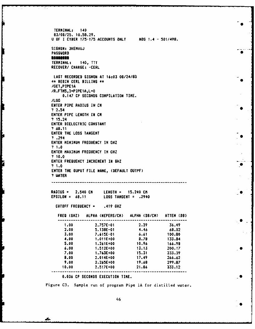
A sample run of each program for distilled water is presented in Figures

C3 and C4. A pipe of radius 1.0 in. (2.54 cm) and length 6 in. (15.24 cm) wasmodeled. Table C2 lists the relative dielectric constants and loss tangents

used for the frequency band of 1.0 to 10.0 GHz. These values were

interpolated linearly from data given by von Hippel for 300 MHz, 3 GHz, and 10

CHz. 9 Because Program Pipe IA uses one relative dielectric constant and oneloss tangent for a band of frequencies, the average value of these parameters

over the frequency band of 1.0 GHz to 10 GHz was used.

Table C3 is a summary of the attenuation output data generated by theseprograms. Note that between I and 5 0Hz, Pipe IB predicts less attenuationthan Pipe IA and vice-versa between 6 and 10 0Hz. This occurs because

attenuation is very dependent on loss tangent. Between I and 5 GHz, the losstangent used by Pipe IA is greater than that used by Pipe 1B, resulting in

greater attenuation. Between 6 and 10 GHz, the loss tangent used by Pipe IA

is less than that used by Pipe 1B, resulting in less attenuation.

0

_S

9 A. R. von Hippel.

44

1 • . . . . . . . .. I I b l . . . . . . . . . . . 1 i i i . . . . . . . . . . . . . . . .

Table Cl

Variables Used in Programs Pipe IA and Pipe 1B

Line nos.where defined

Variable Definition (Pipe IA, Pipe IS)

Al Loglo e 66,73

DISP tan 6, Loss tangent 76,98

EPSR cr' Relative dielectric constant 73,93 .

PREQ f, Frequency in GHz 96,(89 or 112) 0

j j, / 64,71

LENGTH 1, Length of pipe in cm 71,80

PI it 63,70

pliP (ha)nm for TEll mode 65,72

RADIUS r, Radius of pipe in cm 68,77

KC k., (ha)ll/r (r in cm) 69,78

KO ko, 21f/30 (f in CH) 97,91

CANMA Y /kc2 - - (1 - jtana) ko0 9s,101ALPHA a, Real part of y 99,102ALPDB Attenuation dn-!B-20 100,103

ATTEN Overall attenuation in dg, ALPDB x 1 101,104

FC Cutoff frequency, 1 29.997925,. 74,962w O/e c

r

Table C2

Relative Dielectric Constants and Loss Tangents for

Distilled Water at 25°C

Frequency Relative dielectric constant Loss tangent(CHO)(€ (tan 6)

r

1.0 77.3 .052

2.0 77.0 .105

3.0 76.7 .157 04.0 73.6 .212

5.0 70.5 .266

6.0 67.4 .321

7.0 64.3 .376

8.0 61.2 .430

9.0 58.1 .485

10.0 55.0 .540 _9

a- 68.11 tan6 = .294

0

45

TERMINAL: 14083/08/25. 10.58.29.U OF I CYBER 173-175 ACCOUNTS ONLY NOS 1.4 - 501/498.

SIGNON: 3KEMVUJPASSUORD

IERMINALZ 140, TTYRECOVER/ CHARGE: -CERL

LAST RECORDED SIGNON AT 16:03 08/24/83:** BEGIN CERL BILLING ** 0/GETPIPE1A/R.FTN5,I=PIPE1A,L=0

0.147 CP SECONDS COMPILATION TINE./LGOENTER PIPE RADIUS IN CH? 2.54ENTER PIPE LENGTH IN CH? 15.24ENTER DIELECTRIC CONSTANT? 68.11ENTER THE LOSS TANGENT? .294 0ENTER MINIMUM FREQUENCY IN GHZ? 1.0ENTER MAXIMUM FREQUENCY IN GHZ? 10.0ENTER FREQUENCY INCREMENT IN GHZ ...? 1.0 .

ENTER THE OUPUT FILE MANE, (DEFAULT OUTPF)' UATER

RADIUS = 2.540 CH LENGTH = 15.240 Ch S

EPSILON = 68.11 LOSS TANGENT = .2940

CUTOFF FREQUENCY = .419 GHZ

FREO (GHZ) ALPHA (NEPERS/CH) ALPHA (DB/CM) ATTEN (DB)

1.00 2.757E-01 2.39 36.492.00 5.138E-01 4.46 68.023.00 7.615E-01 6.61 100.804.00 1.011E+00 8.78 133.845.00 1.261E+00 10.96 166.986.00 1.512E+00 13.13 200.17 07.00 1.763E+00 15.31 233.398.00 2.014E+00 17.49 266.629.00 2.265E+00 19.68 299.87

10.00 2.517E+00 21.96 333.12

0.036 CP SECONDS EXECUTION TIME. 0

Figure C3. Sample run of program Pipe 1A for distilled water.

46

TERMINAL: 11383/08/25. 14.37.56.U OF I CYBER 175-175 ACCOUNTS ONLY NOS 1.4 - 501/496.

SIGNONt 3XENVUJ 0PASSUORDflU.g.TERMINAL: 113, TTYRECOVER/ CHARGE: -CERL

LAST RECORDED SIGNON AT 14:36 08/25/83 -** BEGIN CERL BILLING **/GET,PIPE1D/R.FTN5,I=PIPE1BL=O

0.134 CP SECONDS COMPILATION TINE./LGOENTER PIPE RADIUS IN CH? 2.54ENTER PIPE LENGTH IN Ch? 15.24ENTER THE OUPUT FILE NAME, (DEFAULT OUTPF)

7 UATER2

ENTER THE FREQUENCY IN GHZ? 1.0ENTER THE DIELECTRIC CONSTANT, DEFAULT 1.00? 77.3ENTER THE LOSS TANGENT, DEFAULT 0.0007 .052

ALPHA = 5.206E-02 NEPERS/CM ( .45 DB)TOTAL ATTENUATION 6.89 DB

--

ENTER THE FREQUENCY IN 6HZ, DEFAULT 1.000ENTER 0 TO QUIT? 2.0ENTER THE DIELECTRIC CONSTANT, DEFAULT 77.30? 77.0ENTER THE LOSS TANGENT, DEFAULT .0527 .105

ALPHA = 1.965E-01 NEPERS/CR ( 1.71 DD)TOTAL ATTENUATION 26.02 D

Figure C4. Sample run of Program Pipe 1B for distilled water.

470

ENTER THE FREQUENCY IN GHZ, DEFAULT 2.000 -ENTER 0 TO QUIT? 3.0

ENTER THE DIELECTRIC CONSTANT, DEFAULT 77.00? 76.7ENTER THE LOSS TANGENT, DEFAULT .105' .157 S

ALPHA = 4.344E-01 NEPERS/CN ( 3.77 DB)TOTAL ATTENUATION = 57.50 DB

ENTER THE FREQUENCY IN 6HZ, DEFAULT 3.000ENTER 0 TO QUIT? 4.0 0

ENTER THE DIELECTRIC CONSTANT, DEFAULT 76.70? 73.6ENTER THE LOSS TANGENT, DEFAULT .157? .212

ALPHA = 7.614E-01 NEPERS/CN 6.61 11)TOTAL ATTENUATION = 100.79 D9

ENTER THE FREQUENCY IN GHZ, DEFAULT 4.000ENTER 0 TO QUIT? 5.0ENTER THE DIELECTRIC CONSTANT, DEFAULT 73.60? 70.5 0

ENTER THE LOSS TANGENT, DEFAULT .212? .266

ALPHA = 1.163E+00 NEPERS/Ch (10.10 DE)TOTAL ATTENUATION = 153.98 DB

ENTER THE FREQUENCY IN GHZ, DEFAULT 5.000ENTER 0 TO QUIT?6.0

ENTER THE DIELECTRIC CONSTANT, DEFAULT 70.50? 67.4ENTER THE LOSS TANGENT, DEFAULT .266'.321 0

Figure C4. (Cont'd).

48

• i l ' " .. . . . . . . .. I ll I I - - • . . . . . . . . . .. . . . . . . . . . -0

ALPHA = 1.639E+00 NEPERS/CN (14.24 DO)TOTAL ATTENUATION= 216.99 DB

ENTER THE FREQUENCY IN 6HZ, DEFAULT 6.000ENTER 0 TO QUIT? 7.0ENTER THE DIELECTRIC CONSTANT, DEFAULT 67.40? 64.3ENTER THE LOSS TANGENT, DEFAULT .321? .376

ALPHA = 2.177E+00 NEPERS/Ch (18.91 DI)TOTAL ATTENUATION = 288.20 09

ENTER THE FREQUENCY ZN OHZ, DEFAULT 7.000ENTER 0 TO QUIT?8.0ENTER THE DIELECTRIC CONSTANT, DEFAULT 64.30? 61.2ENTER THE LOSS TANGENT, DEFAULT .376?.43 o

ALPHA = 2.762E+00 NEPERS/CM (23.99 DB)TOTAL ATTENUATION = 365.57 DB

0

ENTER THE FREQUENCY IN 6HZ, DEFAULT 8.000ENTER 0 TO QUIT? 9.0ENTER THE DIELECTRIC CONSTANT, DEFAULT 61.20? 58.1ENTER THE LOSS TANGENT, DEFAULT .430? .485

Figure C4. (Cont'd).

49I1

ALPHA = 3.395Z+00 NEPERS/CN (29.49 DD)TOTAL ATTENUATION = 449.39 DI

---------- ---------------- ----------------------------

ENTER THE FREQUENCY IN 6HZ, DEFAULT 9.000ENTER 0 TO QUIT? 10.0ENTER THE DIELECTRIC CONSTANT, DEFAULT 58.107 55.0ENTER THE LOSS TANGENT, DEFAULT .4857 .54

ALPHA = 4.061E+00 NEPERS/Ch (35.28 DD)

TOTAL ATTENUATION = 537.63 DI

---------------------------------------------

ENTER THE FREQUENCY IN 6HZ, DEFAULT 10.000ENTER 0 TO QUIT?0

0.062 CP SECONDS EXECUTION TINE./BYE

3KENUUJ COSTS: 61.219 SRUS AT $.0059 = $.36

S

Figure C4. (Cont'd).

500

Table C3

Summary of Output From Sample Runs*

Atten (dB)Frequency Pipe IA Pipe 1B(CHz) (Constant r and tan 6) (Variable E and tan 6)

r r

1.0 36.49 6.892.0 68.02 26.023.0 100.80 57.504.0 133.84 100.795.0 166.98 153.986.0 200.17 216.99 07.0 233.39 288.208.0 266.62 365.579.0 299.87 449.39

10.0 333.12 537.63

*See Figures C3 and C4.

51

APPENDIX D:

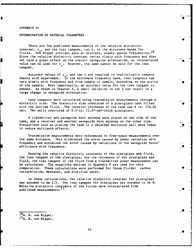
DETERMINATION OF MATERIAL PARAMETERS

There are few published measurements of the relative dielectricconstant, r' and the Loss tangent, tan 6, in the microwave bands forfluids. Von Hippel provides data at discrete, widely spaced frequencies.1 0

Since the relative dielectric constant varies slowly with frequency and doesnot have a great effect on the overall waveguide attenuation, an interpolated -

value can be used for e . However, the same cannot be said for the losstangent.

Accurate values of e , and tan 6 are required to realistically comparetheory with experiment. fn the microwave frequency band, loss tangents canvary widely with frequency and from sample to sample, depending on the purity Sof the sample. Most importantly, an accurate value for the loss tangent isneeded. As shown in Chapter 3, a small variation in tan 6 can result in alarge change in waveguide attenuation.

Loss tangents were calculated using transmission measurements through adielectric slab. The dielectric slab consisted of a plexiglass tank filled Swith the desired fluid. The interior thickness of the tank was 6 in. (15.24cm). The walls consisted of 0.5-in. (l.27-cm)-thick plexiglass.

A transmitter and waveguide horn antenna were placed on one side of thetank, and a receiver and another waveguide horn antenna on the other side.Precautions such as placing the tank in a shielded enclosure wall were taken S

to reduce multipath effects.

Transmission measurements were referenced to free-space measurements overthe same distance. This eliminated the error caused by power variation withfrequency and minimized the error caused by variations in the waveguide horns'efficiency with frequency.

Knowing the relative dielectric constants of the plexiglass and fluid,the loss tangent of the plexiglass, and the thickness of the plexiglass andfluid, the loss tangent of the fluid from a transmitted power measurement canbe calculated. The equations derived in Appendix F are used for thiscomputation. These calculations were performed for three fluids: carbon Stetrachloride, methanol, and distilled water.

In these calculations, the relative dielectric constant for plexiglasswas assumed to be 2.5. The loss tangent for plexiglass was assumed to be 0.Relative dielectric conTiants of the fluids were interpolated from

published measurements.

10A. R. von Hippel.11A. R. von Hippel.

52

Tables DI through D3 list the measured values of tan 6 along with thepublished values. The measured values of tan 6 were consistently lower than

the published values, except for carbon tetrachloride, for which the losstangent was too small to measure by the above method. The discrepancy is

probably explained by the nonidea conditions of the experiment. The 0

theoretical analysis was based on plane wave propagation and infinite slabswhereas the measurements were performed with horn antennas and a finite slab.

To estimate a more accurate value of the loss tangent, the measuredvalues of tan 6 were used to show the trend (shape of the curve) of the

data. The published data provide a reference level. The last column of 6Tables Dl and D2 contains the corrected values of loss tangents. For carbontetrachloride, the published value was used throughout the band.

Table Dl0

Relative Dielectric Constant and Loss Tangent Datafor Carbon Tetrachloride*

Frequency tan 6 S(CH7) r Published*** Measured** Correctedr

2.5 2.17 0.00043.0 2.17 0.0004 0.00043.5 2.17 0.0004 54.0 2.17 0.00044.5 2.17 0.00045.0 2.17 0.00045.5 2.17 0.00046.0 2.17 0.00046.5 2.17 0.0004 S7.0 2.17 0.00047.5 2.17 0.0004

8.0 2.17 0.0004

*Relative dielectric constants obtained by interpolation. -**Unable to measure.***From A. R. von Hippel.

53

Table D2

Relative Dielectric Constant and Loss Tangent Data for Methanol*

Frequency tan 6(GHz) E Published** Measured Correctedr

3.0 23.9 0.6403.54.0 24.0 0.218 0.2344.5 24.0 0.199 0.2155.0 24.0 0.173 0.189

Table D3

Relative Dielectric Constant and Loss Tangent Data for Distilled Water*

Frequency tan 6(GHz) C Published** Measured Corrected

2.5 76.8 0.136 0.1523.0 76.7 0.157 0.141 0.1573.5 73.6 0.147 0.1634.0 70.9 0.126 0.142 S4.5 68.5 0.111 0.1275.0 66.4 0.087 0.1045.5 64.5 0.071 0.0876.0 62.7 0.064 0.0806.5 61.1 0.058 0.0747.0 59.6 0.062 0.078 S

*Relative dielectric constants were obtained by interpolation.**From A. R. von Hippel.

54

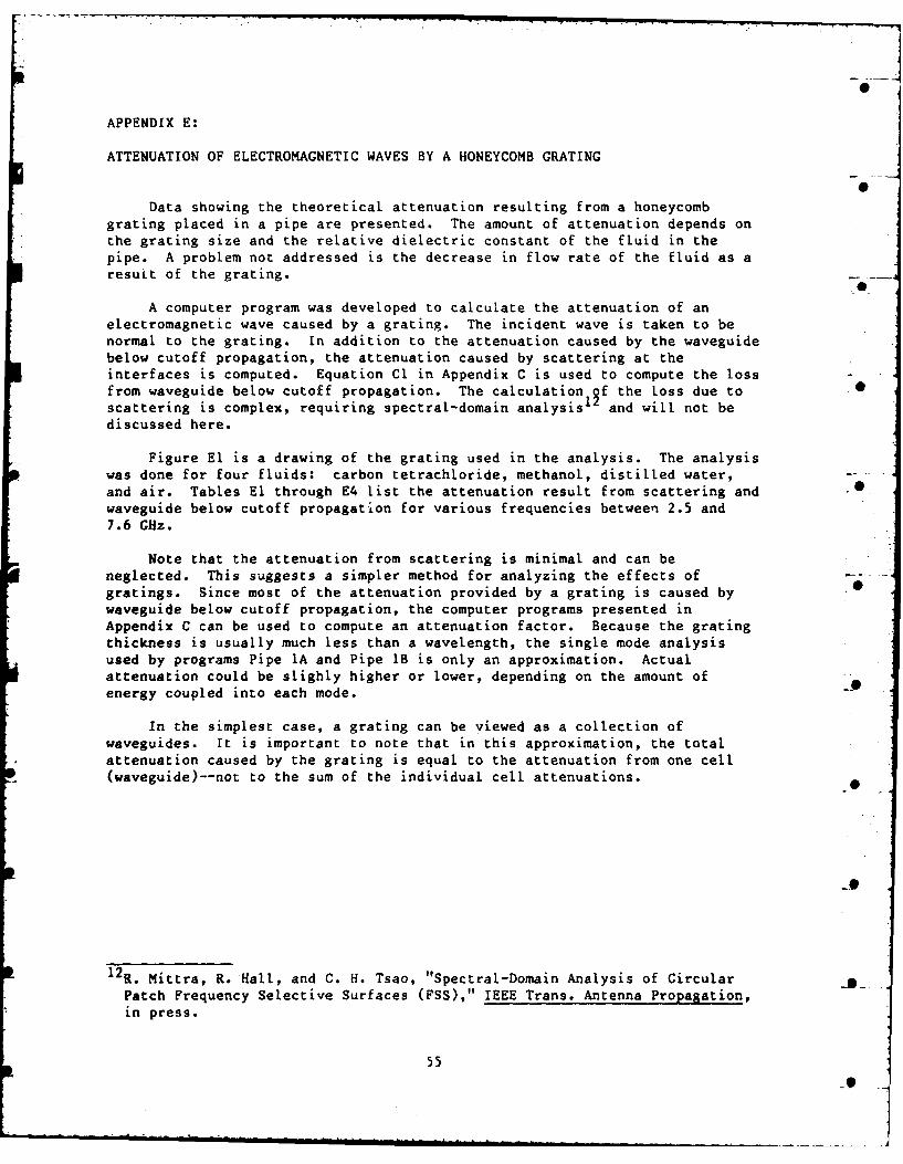
APPENDIX E:

ATTENUATION OF ELECTROMAGNETIC WAVES BY A HONEYCOMB GRATING

0

Data showing the theoretical attenuation resulting from a honeycombgrating placed in a pipe are presented. The amount of attenuation depends on

the grating size and the relative dielectric constant of the fluid in thepipe. A problem not addressed is the decrease in flow rate of the fluid as a

resuLt of the grating.

A computer program was developed to calculate the attenuation of anelectromagnetic wave caused by a grating. The incident wave is taken to benormal to the grating. In addition to the attenuation caused by the waveguide

below cutoff propagation, the attenuation caused by scattering at theinterfaces is computed. Equation Cl in Appendix C is used to compute the lossfrom waveguide below cutoff propagation. The calculationof the Loss due to 0scattering is complex, requiring spectral-domain analysis and will not bediscussed here.

Figure El is a drawing of the grating used in the analysis. The analysis

was done for four fluids: carbon tetrachloride, methanol, distilled water, ..and air. Tables El through E4 list the attenuation result from scattering and 0waveguide below cutoff propagation for various frequencies between 2.5 and7.6 GHz.

Note that the attenuation from scattering is minimal and can be

neglected. This suggests a simpler method for analyzing the effects ofgratings. Since most of the attenuation provided by a grating is caused bywaveguide below cutoff propagation, the computer programs presented inAppendix C can be used to compute an attenuation factor. Because the gratingthickness is usually much less than a wavelength, the single mode analysisused by programs Pipe IA and Pipe lB is only an approximation. Actual

attenuation could be slighly higher or lower, depending on the amount ofenergy coupled into each mode.

In the simplest case, a grating can be viewed as a collection ofwaveguides. It is important to note that in this approximation, the totalattenuation caused by the grating is equal to the attenuation from one cell(waveguide)--not to the sum of the individual cell attenuations.

12R. Mittra, R. Hall, and C. H. Tsao, "Spectral-Domain Analysis of Circular

Patch Frequency Selective Surfaces (FSS)," IEEE Trans. Antenna Propagation,in press.

55

LI= 0.5"

0000* 2a -0.15"000 ......

S1.85" OIA.

Figure El. Diagram of the honeycomb grating used in calculating the

attenuations in Tables El, E2, E3, and E4.

Table El

Calculated Attenuation Factors Resulting From a Honeycomb Grating:Carbon Tetrachloride

Attenuation fromFrequency Attenuation from waveguide below

(GHz) scattering cutoff propagation

2.5 .015 106.1

3.0 .024 106.03.5 .033 105.8 04.0 .044 105.64.5 .055 105.45.0 .068 105.1

5.5 .083 104.86.0 .099 104.56.5 .116 104.2 _7.0 .135 103.8

7.5 .155 103.4

56 S

Table E2

Calculated Attenuation Factors Resulting From a Honeycomb Grating: Methanol

Attenuation from 0

Frequency Attenuation from waveguide below

(GHz) scattering cutoff propagation

4.0 .044 96.44.5 .055 93.6

5.0 .068 90.3

Table E3

Calculated Attenuation Factors Resulting From a Honeycomb Grating: SDistilled Water

Attenuation from

Frequency Attenuation from waveguide below

(GHz) scattering cutoff propagation

2.5 .015 93.6

3.0 .024 87.53.5 .033 79.94.0 .044 70.34.5 .055 57.9

5.0 .068 40.65.5 .083 16.16.0 .099 11.1

6.5 .116 6.4

7.0 .135 6.47.5 .155 5.2

7.6 .159 5.0

Table E4

Calculated Attenuation Factors Resulting From a Honeycomb Grating: Air

Attenuation from

Frequency Attenuation from waveguide below

(GHz) scattering cutoff propagation

2.5 .015 106.3

3.0 .024 106.2 -03.5 .033 106.2

4.0 .044 106.1

4.5 .055 106.0

5.0 .068 105.8

5.5 .083 105.76.0 .099 105.66.5 .116 105.4

7.0 .135 105.2

7.5 .155 105.1

57

APPENDIX F:

TRANSMISSION OF ELECTROMAGNETIC WAVES THROUGH MULTIPLE DIELECTRICS

0

Consider the problem of wave propagation through a multilayered

dielectric region (Figure Fl). Each Layer has relative dielectric constant

(possibly complex) e = E., i = 1, 2, ..., N and lies between z = zi l and z i

where z= - and zN +.! A TEM wave, propagating in the +z direction, isincident from the left. In the ith region, the electric and magnetic fields

(Ei and Hi ) are given by

-jk.z +jk z

E. = T. (e i + R.e ) [Eq FI-jk.z +jk z

H. = T.Y. (e - R.e ) [Eq F21

where

Y. = /- Y [Eq F3]I 1 0

k. = ore-. k (Eq F4]

Y and k are the free-space wave impedance and wave number, respectively. T.is the transmission coefficient in the ith region. R. is the ith reflection

coefficient. Since regions 1 and N are unbounded, Ti1= 1 and RN = 0.

Forcing the continuity of E and H at the interface between the ith and

the (i + l)th layer, the following relationship results:

-jk~z. jk.z1 1i z T]

e e i

L -jkiz i -Yi+1 e 1 i TkR

e eJki+iZi +jki+zi Ti+l [Eq F51i -kle lz Yi e •j ~ iT + ~

i+1 e~ 1 , 2 , .. , N -1. ..

If we then define:

X. =lgF]

-jk.z. +jk.z. TiR [Eq 6]

Ai,j Le -jk z e i [Eq F71i i j +jk z-

58

- . . . . . . . . ." -" . . .- - - - " I I I ] n i . . . n nn m n | r i - -nn -- - - . . . . 1 . .

, . . _ . . .

' I J~ 2 ,E~, NJ-o'11',' AO 4 ""0 ON "" "

60 > 0,'L

(FREESPACE) -

El H

" ETer

M ..i- .....

Z-O Z-Z1 Z2 ZNI ZN

Figure Fl. TEM wave propagation through a multilayered dielectric region.

Equation F4 can be rewritten as:

Ai i Xi = Ai+l, i Xi+ 1 i = 1, 2, ... , N-I (Eq F81

Solving for Xi+l:

(Ai+,i Ai i = Xi+ [Eq F9

Equation F9 relates the reflection and transmission coefficients in the ithregion to the reflection and transmission coefficients in the (i+l)th regionby a matrix equation. These matrices can be cascaded to relate XI to XN.

X.=NL ) Ai, X. [Eq FIO]

The bracketed quantity in Equation FlO is a 2x2 matrix, depending only onknown quantities. As T =1 and R5=0 for the dielectric slab measurement,Equation F1O consists ttwo equations and two unknowns, R1 and T5, theoverall reflection and transmission coefficients. Equation FIO can be solvedfor R, and T5 . The matrix product in Equation FI0 can be carried outanalytically, although for large N values, this is difficult. It is oftenmore convenient to calculate the matrix product numerically.

When one or more of the regions is particularly lossy and is more thanseveral wavelengths long, certain numerical problems can arise in computingEquation Fl0. In this case, the A- matrices in the ith layer consist of bothvery large and very small numbers.14o evaluate the matrix product in EquationFIO, these numbers must be multiplied and added. This can yield inaccurateresults when using finite precision arithmetic. This problem can be avoided

59

. . . . = .. _ . . .0

by using double precision arithmetic or using a computer with a longer wordlength. A second solution to the problem is obtained analytically by ignoringthe heavily attenuated reflected terms.

40

60mi

CITED REFERENCES

Abramovitz, M., and I. Stegun, Handbook of Mathematical Functions (Dover

Press, 1970). 0

Collin, R. F., Field Theory of Guided Waves (McGraw-Hill Co., 1960).

Collin, R. F., and F. J. Zucker, Antenna Theory, Part I (McGraw-Hill Co.,1969).

DASA EMP Handbook, DASA 2114-1 (Defense Atomic Support Agency [DASA]

Information and Analysis Center, September 1968).

DNA EMP Awareness Course Notes, Third Ed., DNA 2i72T (Defense Nuclear Agency,October 1977).

EMP Engineering Practices Handbook, NATO file No. 1460-2 (October 1977).

Kraus, J. D., Antennas (McGraw-Hill Co., 1950).

Marcuvity, N. (ed.), Waveguide Handbook (McGraw-Hill Co., 1951).

Measurement of Shielding Effectiveness of High-Performance ShieldingEnclosures, Institute of Electrical and Electronic Engineers (IEEE) Method299 (1975).

Method of Attenuation Measurements for Enclosures, Electromagnetic Shielding,

for Electronic Test Purposes, MIL-STD-285 (Department of Defense, June1 75).

Mittra, R., R. Hall, and C. H. Tsao, "Spectral-Domain Analysis of CircularPatch Frequency Selective Surfaces (FSS)," IEEE Trans. AntennaPropagation, in press.

Nuclear Electromagnetic Pulse (NEMP) Protection, TM 5-855-5 (Headquarters,Department of the Army, February 1974).

Pearson, J. D., "The Diffraction of Electro-Magnetic Waves by a Semi-InfiniteCircular Wave Guide," Proceedings of the Cambridge Philosophical Society,Vol 49, Part 4 (1953), pp 659-667.

Ramo, S., J. Whinnery, and T. Van Duzer, Fields and Waves in CommunicationElectronics (John Wiley and Sons, Inc., 1965).

Southworth, G. C., and A. P. King, "Metal Horns as Directive Receivers ofUltra-Short Waves," Proceedings of the I.R.E., Vol 27 (February 1939),pp 99-102.

von Hippel, A. R., Dielectric Materials and Applications (Technology Press ofthe Massachusetts Institute for Technology, 1954).

61

L ..

UNCITED REFERENCE

Decreton, M. C., and N. S. Ramachandraiah, "Nondestructive Measurement of-Complex Permittivity for Dielectric Slabs," TEEE Transactions on MicrowaveTheory Technology (MTT) (December 1975), p 1077.

620

CERL DISTRIBUTION

, if uf Enjineers HnC

ATTN: Tech Htonitor ATTN: HSLO-F 78234

ATTN, nAEN-ASIL !2) ATTN: Facilities Engineer

ATTN, DAEN-(tC) Fitzsimons AMC 80240

ATTN. AA[N-CW Waiter Reed AMC 20012

A(tIN: IIAEN-( V

ATTN. TAEN-iW-i( INSCOM - Ch, Instl. Div.

ATTN. f)(EN-CW) ATTN, Facilities Engineer (3)

AnTN FAEN-CWPATTN. OAN-ECATTN. DAEN-ECC ATN: OEH (3)

ATTN: OAEN-ECEATTN. OAEN-ZCF MTMC

ATTN. DAEN-C( ATTN: 9TC-SA 20315

ATTN: OAEN-RD ATTN: Facilities Engineer (3)

ATTN: 0AEN-ROC

ATTN. OAEN-ROM NARADCOM, ATTN: DROSA-F 071160

ATTN. DAEN-MATTN: DAEN-ZCZ TARCOM, Fac. Div. 48090

ATTN. DAEN-ZCE

ATTN: DAEN-ZCI mAOo -- E

ATTN. DAEN-ZC4 No, TRADOC, ATTN. ATEN-EHATTN. DEH (19)

FESA, ATTN. Library 22060

ATTN. DET 111 79906 TSARCOM, ATTN: STSAS-F 63120

US Army Engineer Districts

ATTN: Library (41) USACC

US Army Engineer Divisions ATTN. Facilities Engineer (2)

ATTN. Library (14) WESTCOI

US Army Europe ATTN: DEH

AEAEN-00CS/Engr 09403 Fort Shatter 96858

ISAE 09081 ATTN: APEN-IM

V CorpsATTNI DEH (11) SHAPE 09055

VT! Corps ATTN. Survivability Section, CCB-OPSATTN. DEN (15 Infrastructure Branch. LANDA

21st Support Command

ATTN, DEH (12) No USEUCOM 09128

USA Berlin ATTN: ECJ 4/7-LOE

ATTN. DEN (15)USASETAF U.S. Army, Fort Belvoir 22060

ATTN, DEH (6) ATTN: Canadian Liaison Officer

Allied CEmmand Europe (ACE) ATTN: Water Resources Support Center

ATTN, DEi (3) ATTN: Engr Studies Center

ATTN: Engr Topographic Lab

8th USA. Korea (14) ATTN: ATZA-DTE-SU

AITN: ATZA-DTE-4M

REK/US Combined Forces Comand 96301 ATN: R & 0 ComlndATTN.kl EUSA-iHC.CFC/EngrA a USANJI

CRREL, ATTN: Library 0375SP. USA Japan (USARJ)

ATTN. AJEN-FE 96343ATTN: DEH-Honshu 96 13

ATTN, DEH-Okinawa 96331 WES, ATTN: Library 39180

HQ, XVIII Airborne Corps and

Ft. Bragg 28307Area Engineer. AEDC-Area Office ATTN. AFZA-FE-EE

Arnold Air Force Station, TN 37389Chanute AFB, IL 618683345 CES/DE. Stop 27

Norton AFB CA 92409

416th Engineer Command 60623 ATTN: AFRCE-MX/DEE

ATTN. Facilities EngineerTyndall AFB, FL 32403

US Military Academy 10966 AFESC/Engineering & Service LabATTN. Facilities Engineer

ATTN: Dept of Geography & NAVFACComputer Science ATTN: RDTLE Liaison Office (6)

ATTN. DSCPER/MAEN-A ATTN, Sr. Tech. FAC-03T 22332ATTN. Asst. COR R&D. FAC-03 22332

AMMC. ATTN: ORXMR-WE 02172 NCEL 93041

USA ARRCOH G1299 ATTN, Library (Code LOBA)ATTN . IS-RIT-"ATTN. ORSAR-IS Defense Technical Info. Center 22314

ATTN ORSR-ISATTNt DDA (12)

CARCON' -ODir., * nst.,,& Svcs.ATTN. DE (23) Engineering Societies LibraryWew York. NY 10017

OLA ATTN. OLA-lil 2231dNational Guard Bureau 20310

FORSCOM Installation Division

FORSCOM Engineer, ATTN: AFIN-DEHATTN. DEH (23) US Government Printing Office 22304

Receiving Section/Depository Copies (2)

US Army Env. Hygiene AgencyATTN.: HSHB-E 21010National Bureau of Standards 20760

1009i/V/Rd

EMS Team Distribution 0

Chief of Engineers 20314 US Army Engineer District Ft. Leavenworth, KS 66027ATTN: DAEN-MPZ-A Seattle 98124 ATTN: ATZLCA-SAATTN: DAEN-MPO-B ATTN: Chief, NPSCOATTN: DAEN-MPO-U ATTN: Chief, EN-DB-EM Ft. Lee, VA 23801

ATTN: Chief. EN-DB-ST ATTN: DRXMC-D (2)US Army Engineer District ATTN: Chief, NPSEN-PL-WC

New York 10007 Walla Walla 99362 Ft. McPhersor., GA 30330 SATTN: Chief, Design Br. ATTN: Chief, Engr Div ATTN: AFEN-CD

Pittsburqh 15222 Alaska 99501ATTN: Chief. Engr Div ATTN: Chief, NPASA-R Ft. Monroe, VA 23651

Philadelphia 19106 ATTN: ATEN-AD (3)ATTN: Chief, NAPEN-D US Army Engineer Division ATTN: ATEN-FE-BG (2)

Baltimore 21203 New England 02154 ATTN: ATEN-FE-WATTN: Chief, Engr Div ATTN: Chief, NEDED.T

Norfolk 23510 Middle East (Rear) 22601 Aberdeen Proving Ground, MD 21005 -ATTN: Chief, NAOEN-M ATTN: Chief, MEDED-T ATTN: ANXHEATTN: Chief, NAOEN-D North Atlantic 10007

Huntington 25721 ATTN: Chief, NADEN-T Harry Diamond Labs 20783ATTN: Chief, ORHEO-D South Atlantic 30303 ATTN: DELHD-NW-E

Wilmington 29401 ATTN: Chief, SADEN-TS ATTN: OELHD-NW-EAATTN: Chief, SAWEN-OS ATTN: Chief, SADEN-TE/TM ATTN: DELHD-NW-ECATTN: Chief, SAWEN-D Huntsville 35807 ATTN: DELHD-NW-ED

Charleston 20402 ATTN: Chief, HNDED-CS ATTN: DELHD-NW-EEATTN: Chief, Enqr Div ATTN: Chief, HNDED-ME

Savannah 31402 ATTN: Chief, HNDED-SR USA Natick Labs 01760ATTN: Chief, SASAS-L ATTN: Chief, HNOED-FD NARADCOM/DRDNA-UST

Jacksonville 32232 Ohio River 45201ATTN: Const Div ATTN: Chief, Engr Div USA-WES 39180ATTN: Design Br., Structures Sec. North Central 60605 ATTN: C/Structures

Mobile 3662R ATTN: Chief, Engr DivATTN: Chief, SAMEN-D Missouri River 68101 NAVFAC/Code 04ATTN: Chief. SAMEN-C ATTN: Chief, MRDED-T Alexandria, VA 22332

Nashville 37202 Southwestern 75202ATTN: Chief, ORNED-D ATTN: Chief, SWOED-TS Naval Air Systems Command 20360 5

Memphis 39103 ATTN: Chief, SWDED-TM ATTN: LibraryATTN: Chief, LMMED-DT South Pacific 94111ATTN: Chief, LMMED-DM ATTN: Chief, SPDEO-TG Naval Training Equipment Command 32813

Vicksburg 391qO Pacific Ocean 96858 ATTN: Technical LibraryATTN: Chief, Enqr Div ATTN: Chief, Engr Div

Louisville 40201 ATTN: Chief, FM&S Branch Port Hueneme, CA 93043ATTN: Chief, Enqr Div ATTN: Chief, POOED-D ATTN: Morel) Library

Detroit 48231 North Pacific 97208ATTN: Chief, NCEED-T ATT: Chief, Engr Div Boling AFB, DC 20332

St. Paul 55101 AF/LEEEUATTN: Chief, ED-D 6th US Army 94129

Chicago 60604 ATTN: AFKC-EN AFE, Camp HumphreysATTN: Chief, NCCED-DS APO San Francisco 96721

Rock Island 61201 7th US Army 09407ATTN: Chief, Engr Div ATTN: AETTM-HRO-EHD Griffiss AFB 13440ATTN: Chief, NCRED-D RADC/RBES

St. Louis 63101 HQ, Combined Field Army (ROK/US) 96358ATTN: Chief, ED-D ATTN: CFAR-EN Hanscom AFB. MA 01731 0

Kansas City 64106 ATTN: HQ AFSC

ATTN: Chief, Enqr Div US Army Foreign Science & Tech. Center ATTN: ESD/OCR-3Omaha 6102 ATTN: Charlottesville, VA 22901

ATTN: Chief, Engr Div ATTN: Far East Office 96328 Kirtland AFB, NM 87117New Orleans 70160 ATTN: AFWL/DES

ATTN: Chief, LMNED-DG USA Liaison Detachment 10007 ATTN: AFWL/DYCLittle Rock 72203 ATTN: Library

ATTN: Chief, Enqr Div Little Rock AFB 72076

Tulsa 74102 USA ARRADCOM 07801 ATTN: 314/DEEEATTN: Chief, Enqr Div ATTN: DRDAR-LCA-OK

Fort Worth 76102 Patrick AFB, FL 32925ATTN: Chief, SWFED-O CERCOM, Ft. Monmouth 07703 ATTN: XRO

Galveston 77550 ATTN: DRSEL-LE-SSATTN: Chief, SWGAS-L Tinker AFB, OK 73145ATTN: Chief, SWGED-OS Defense Nuclear Agency 20305 2854 ABG/DEEEATTN: Chief, SWGED-DM ATTN: DNA-RAEE

Albuquerque 97103 ATTN: ONA-STRA Tyndall AFB, FL 32403ATTN: Chief, Engr Div ATTN: ONA-DOST ATTN: AFESC/TBT

Los Angeles 90053 ATTN: DNA-RAEV ATTN: AFESC/RDCFATTN: Chief, SPLED-D

San Francisco 94105 SHAPE 09055 Wright-Patterson AFB, OH 45433ATTN: Chief, Engr Div Chief, Land & Msl. lnstl. Section ATTN: ASO/ENAMA

Sacramento 95814 ATTN: AFWAL/MLSEATTN: Chief, SPKED-D Ft. Belvoir, VA 22060

Far East 96301 ATTN: Learning Resources Center Bldg. Research Advisory Board 20418ATTN: Chief, Engr Div ATTN: ATSE-TD-TL (2) Dept. of Transportation Library 20590

Portland 9720 Transportation Research Board 20418ATTN: Chief, OB-6 Fort Clayton, Canal Zone 34004ATTN: Chief, 08-3 ATTN: OFAE Airports and Const. Services Dir.

Technical Info. Reference Centre

Ottawa, Canada KIA ONO

1+5

2.1.82

The effect of fluids on waveguides below cutoff penetrations as related toelectromagnetic shielding effectiveness / by Michael K. McInerney ...(at al.) - Champaign, Il Construction Engineering Research Labora-tory, 1984.62 p. (Technical report / Construction Engineering Research Labora-tory ; M-354).

1. Shielding (electricity). 2. Wave guided. 3. Fluids. L. Mclnerney,Michael K. IZ. Ray. Scott, I1. McCoruack, Kaymond G. LV. :asmtillv, Stuve.V. Mittre, Raj. Vi. Series; Technical report (Construction EngineeringResearch Laboratory) ;.M-354.

01

I

_0

i_

0