Embed Size (px)
Citation preview

AD-AL16 #166 OFFICE OF NAVAL RESEARCH ARLINGTON VA F/B 15/5I AR8NAVAL RESEARCH LOGISTICS QUARTERLY. VOLUME 29, NUMBER I.dW
UNIELAEEEEIEEEEI
NfHVRL RESEFRCHp LOGISTICSo QUARTERLY Q4
m
MARCH 1982 *
VOL 29, NO.I
>....- AV-LJ
OFFICE OF NAVAL RESEARCH
82 06 21 2 SAo P-1278
NAVAL RESEARCH LOGISTICS QUARTERLY
EDITORIAL BOARD
Marvin Denicoff, Office of Naval Research, Chairman Ex Officlo Members "Ac c r •
Murray A. Geisler, Logistics Management Institute Thomas C. Varley, Office of 1A ntl ResearchProgram Director
W. H. Marlow, The George Washington University Seymour M. Selig, Office of val ResearchManaging Editor
MANAGING EDITOR DT1_
Seymour M. Selig 00"
Office of Naval Research aAArlington, Virginia 22217
ASSOCIATE EDITORSFrank M. Bass, Purdue University Kenneth 0. Kortanek, Carnegie-Mellon Universi,Gabriel R. Bitran, Massachusetts Institute of Technology Charles Kriebel, Carnegie-Mellon UniversityJack Borsting, Department of Defense Jack Laderman, Bronx, New YorkEric Denardo, Yale University Gerald J. Lieberman, Stanford UniversityMarco Fiorello, Logistics Management Institute Clifford Marshall, Polytechnic Institute of New YorkMartin J. Fischer, Defense Communications Agency Richard C. Morey, Duke UniversitySaul I. Gass, University of Maryland John A. Muckstadt, Cornell UniversityNeal D. Glassman, Office of Naval Research William P. Pierskalla, University of PennsylvaniaPaul Gray, Southern Methodist University Thomas L. Saaty, University of PittsburghCarl M. Harris, Center for Management and Henry Solomon, The George Washington University
Policy Research Wlodzimierz Szwarc, University of Wisconsin, MilwaukeeAlan J. Hoffman, IBM Corporation James G. Taylor, Naval Postgraduate SchoolUday S. Karmarkar, University of Rochester Harvey M. Wagner, The University of North CarolinaPaul R. Kleindorfer, University of Pennsylvania John W. Wingate, Naval Surface Weapons Center, White OakDarwin Klingman, University of Texas, Austin Shelemyahu Zacks, State University of New York at
Binghamton
The Naval Research Logistics Quarterly is devoted to the dissemination of scientific information in logistics andwill publish research and expository papers, including those in certain areas of mathematics, statistics, andeconomics, relevant to the over-all effort to improve the efficiency and effectiveness of logistics operations.,
Information for Contributors is indicated on inside back cover.
The Naval Research Logistics Quarterly is published by the Office of Naval Research in the months ofMarch, June, September, and December and can be purchased from the Superintendent of Documents,U.S. Government Printing Office, Washington, D.C. 20402. Subscription Price: $15.00 a year in theU.S. and Canada, $18.75 elsewhere. Cost of individual issues may be obtained from the Superintendentof Documents.
The views and opinions expressed in this Journal are those of the authors and not necessarily thosethe Office of Naval Research.
The Naval Research Logistics Quarterly is published from appropriated funds by authority of the Office ofNaval Research in accordance with NPPR P-35. Controlled circulation postage paid at Washington and addi-tional mailing offices. Articles, letters and address changes may be forwarded to Department of the Navy, Of-rice of Naval Research, Ballston Tower# 1. Roo , 6 ,800 N. Quincy St., Arlington, VA. 22217.
r- . . . . .
&A THEORY OF MULTISTAGE CONTRACTUAL INCENTIVES
WITH APPLICATION TO DESIGN-TO-COST
Robert W. BlanningOwen Graduate School of Management
Vanderbilt University
Nashville, Tennessee
Paul R. Kleindorfer
Department of Decision SciencesThe Wharton School
University of PennsylvaniaPhiladelphia, Pennsylvania ",
C . S, Sankar t ". ,
Computer and Information Sciences Dept. . , , , -
Temple UniversityPhiladelphia, Pennsylvania
1. INTRODUCTION
A topic of increasing importance in public-sector management is the design and implementationof financial incentive systems that will encourage lower-level government units and profit-makingorganizations under contract to these units to use government funds efficiently and qatisfy nonfinancialgovernment objectives. One such incentive system is the Design-to-Cost (DTC) system, implementedfor many major weapons acquisition projects in the Department of Defense [5], [141 in which a DTCgoal is established for each project. Any deviations from the goal are corrected by changing the perfor-mance of the weapons system or by changing the number of weapons produced, or both. This paperconstructs a simple model of the information, incentive and decision aspects of such an incentive sys-tem and offers insights into the tradeoffs and policy issues involved.
There is substantial literature on the theory of contracts [151, [81 and the design of incentives [2],[61, [7], 110], 19]. However, an examination of this literature discloses the need for research in twoareas that are essential to an understanding of the weapons acquisition process. The first need ariseswhenever a development effort precedes a production effort. The dynamic incentive process-that is, amultistage process in which contractor behavior during any one stage is affected, by the incentivesoperative during that stage, and by an expectation of rewards or punishments in the subsequentstages-is not addressed by the literature. The second need arises due to lack of consideration of anybut the most simple of hierarchies. Yet in any large government/contractor effort, the government isrepresented by at least three distinct organizations (the Congress, the Administration, and the Bureau-cracy), and the contracting agent may be represented by several organizations as well (e.g., contractorsand subcontractors). This paper addresses both the dynamic and hierarchical aspects of contracting inthe DTC context (see [121, [11).
The weapons acquisition process is viewed here as a multistage process whose characteristicschange substantially over time. The acquisition process consists of (at least) three steps: (1) adevelopment stage in which two or more contractors receive funds to design and test a prototypeweapon, at the end of which a single contractor is awarded a production contract; (2) a production stagein which the winning contractor produces one or more copies of the weapon; and (3) an implementa-tion and maintenance stage in which the weapon is maintained and modified in the field, often withsome contractor support. The principal interactions occur between the first two stages (i.e., contractorsbehave differently during the development stage as the award of the production contract is uncertain).
VOL. 29, NO. I, MARCH 1982 1 NAVAL RESEARCH LOGISTICS QUARTERLY

2 R. W. BLANNING, P. R. KLEINDORFER AND C. S. SANKAR
Hence, we will confine our analysis to the first two stages. We assume that the contract duringdevelopment stage is a fixed-price contract and the contract during production stage is an incentive con-tract including (1) full cost recovery, (2) a reward or penalty depending on the cost of productionrelative to a negotiated cost target, and (3) a reward or penalty depending on weapon performance rela-tive to a prespecified performance target.
The hierarchical nature of the DTC system is also emphasized in our research. We examine fourlevels of government and contractor hierarchy. At the highest level, representing the Congress and theAdministration. DTC goals and allowable probabilities of exceeding these goals are established.(Weapon cost and performance are assumed to be random variables whose mean values are controll-able.) At the second level, representing DoD and the appropriate military service, the DTC goal is par-titioned into two subgoals, one for the development stage and one for the production stage, and thecontractors participating in the development stage are selected. At the third level, representing the mil-itary service and its project managers, most of the parameters in the incentive system are establishedand the production contract is awarded. (In our analysis, we assume that the decisions at this level areestablished by decision rules known in advance to both the government and the contractors.) At thefourth level, representing the contractors, contract parameters are negotiated and the levels of contrac-tor effort (number of personnel, cost of raw material, etc.) are chosen for the two stages.
In the following section a model of the DTC incentive system is developed. The model is solvedto determine the impact of government decisions (contractual incentive parameters, the allocation ofthe DTC goal between development and production stages, and the level of risk acceptable to thegovernment) and the technological and market environment of the project on outcomes such as thequality of the weapon produced, the cost to the government, the profit of the firms in the industry, therisks assumed by the government and the risks assumed by the firms. Some of the policy implicationsof the model are then illustraJted by a series of examples.
2. THE BASIC MODEL
We consider a given project and assume that Congress has established a Design-to-Cost (DTC)goal, G for the project. G is understood to be a constraint on total project cost and it is assumed that Gmay be exceeded only with ex ante probability y. One might anticipate that DoD would set y strategi-cally to trade off the transactions costs of exceeding budgets and exposing itself to (re) appropriationshearings against the internal transactions costs which occur if -Y is small.
We assume that n firms have been preselected as candidates for carrying out the project, in twostages. In the development stage, the n firms compete against one another in producing the bestdesign. In the second stage, the firm with the best first-stage design is awarded (the opportunity to bidon) a production contract. To state the problem precisely we need the following notation.
e, = Effort expended by firm i in stage s. In the development stage, s = (I, and in theproduction stage, s = p;
Q,,(e,, = Quality (or performance level) achieved by firm i in stage s;*
C, (e=, Costs incurred by firm i in stage s as a function of effort expended.
'We assume that a single measure of quality describes adequately the performance of the system and that (his measure is additiveacross the development and production stages li.e., that development quality plus the quality added during the production stageequals total quality) In practice the measure is multidimensional, and many of the dimensions appropriate to the developmentstage are not the same as those appropriate to the production stage. The former emphasize mission requirements. proper exploi-tation of new technology. etc. The latter emphasive quality Woirol. delivery schedules, etc. We assume thai the government andthe contractor can agree on a procedure (e.g., the calculation of a weighted sum of the various dimensions of quality) thai willresult in a single additive measure.
NAVAL RESEARCH LOGISTICS QUARTERLY VOL. 29. NO. 1, MARCH )992
DESIGN-TO-COST MULTISTAGE CONTRACTUAL INCENTIVES 3
DoD is assumed to consider the following types of contract. All development contracts are firmfixed price contracts with each of the n firms involved receiving Gd/n dollars.* Gd < G is therefore thetotal development cost to the government. The production contract, if awarded to firm i, is assumed tobe a general incentive contract with payments above costs to firm i specified as:
(1) fil, (Tb ,,, 0,,) = a T, + b (T, - e,(e) + R,(od + O,(ei,)),
where random quantities have a - over them, and where
T, = Target cost rate, negotiated by firm i at the beginning of the production stage; T, isassumed constrained to be nonnegative (negative bids are not allowed);
Qd = Cumulative progress in quality of the project during the development stage, which is
the starting point for the production stage;
a,b = Contract incentive parameters, where a >, 0, 0 < b < 1;
R (q) = Performance incentive payment, for firm i, expressed as a function of total qualityachieved over both stages.
At the end of the development stage, DoD would have spent exactly Gd dollars, leavingG= G - Gd dollars in the overall project budget. Suppose firm i achieves the best performance in thedevelopment stage, i.e., suppose
(2) Od,(ed,)-= Qd Max QdJ(edl).I <i < n
We assume that if (2) obtains, then firm i is given the exclusive right to bid on a production contract.In a realistic setting, one might assume that more than one of the leading firms at the end of thedevelopment stage is given the opportunity to bid on a production contract. This possibility is excludedhere. Thus, it is assumed that the leading development firm, say i, is interested at the beginning of theproduction stage in setting T,,, ei, a, and b so as to maximize its profits in development stageU,,(T,, ep,, Qd) where
(3) V,( T, ep,, Qd) -
E{If, (Tfp, e,,, Qd) + F,(Qd,(ed), Op,(ep,)) I d(ed,) = Qd},
where F,(qd,q , ) represents expected follow-on benefits to firm i (e.g., in terms of maintenance con-tracts, future benefits from the technology developed, etc.)t fl, is given in (1), and [flp, + C ,represents total (incentive plus cost) payments made by the government in the production stage.
*In general one would expect some sort of cost reimbursement to take place during the development stage. However. we as-
sume a fixed price contract to contrast firm behavior in this stage with firm response to government-established incentives in theproduction stage. In Sections 5 and 6 we examine the implications of this assumption-primarily, that some firms may decline toparticipate in the development process. This may occur even under cost reimbursement if some firms find that their expectedprofits, although nonnegative, are less than the profits that would result from alternative earnings opportunities.
tIt was mentioned in the introduction that the acquisition process consists not only of a development and a production stage, butalso an ongoing stage of operation and maintenance, including retrofitting and occasionally major modification. We do not expli-citly consider this third stage, so that we may focus more closely on the relationship between development and production.Thus, we are concerned here % I acquisition costs and not with life cycle costs. However, some of this may be captured in thequality measure and the follow-on benefits. That is, the firm that produces a reliable and maintainable system is likely to developa reputation that will lead to significant follow-on benefits. The impact of these follow-on benefits is first explained on page 4 andis discussed in more detail later in the manuscript. (See also footnote on page 7.)
VOL 29, NO 1, MARCP 1982 NAVAL RESEARCH LOGISTICS QUARTERLY
4 R. W. BLANNING, P. R. KLEINDORFER AND C. S. SANKAR
Of course, firm i will be subject to some constraints in indulging with its preferences asrepresented by (3). Indeed, we assume that "d' is fixed in advance by the government and the follow-ing holds for variables (T,,esb):
(4) Pr{I i(Ti, eiQd) + e , G,} < ",
where -y is specified by the Congress and the Administration. The fact that firms accept (4) as a con-straint, of course, presumes that in the case of costs overruns, acceptable auditing practices can exposeand penalize firms which cannot make a credible ex post case that (4) was observed in their planning.This dependence of contractual incentives on (legitimate) enforcement and monitoring procedures can-not be overemphasized.
Beyond fixing "a" and imposing (4), we will assume that production contracts are negotiatedthrough one of two methodst (firm i is the leading development firm):
Method 1, MI: "b" is fixed ex ante and any Tp,.ep, satisfying (4) will be accepted by DoD.
Method 2, M2: Firm i and DoD negotiate ( T,,.e,,,b) at the beginning of the production stagesuch that (4) is satisfied and such that a Pareto efficient point is reached between firm i and [)ol). Thepreferences of firm i are represented by (3). DoD is assumed to have preferences represented by autility function UD(C,CO,Q), where Q = Qd + 0,,(e,,,) is final project quality, C = G" + li, + (C, istotal project cost, and CO = C - G is the cost overrun.
Formally, we may represent the two production stage decision processes just described as follows:
(5) MI: Maximize (3) with respect to (7T,.e,,), subject to (4).
(5') M2: Maximize Ia-U i(T,,e,,,Qa ) +
(1-a)E(UD(Gd + FP, + C P,, Gd + fl,,, + - G, Q, + 0,,(e,,)l
subject to (4), T,, > 0, e,,, > 0 and 0 < b < 1,
where a is between 0 and I and reflects the relative bargaining power of the contractor against Dol),Up, is defined in (3), 1,, is given in (I), C,, = C,, (e,,,) is the cost for the production stage, and Qj isthe observed realization of (2). We will define the optimal solution value to (5) or (5') as 11,,(Q): thisis the optimal expected return for firm i if the ending quality level in (2) is Q, and firm i is awa ded theproduction contract.
Now consider the development stage. Each of the n firms involved may be assumed to maximizethe sum t of present benefits and expected follow-on benefits ( '7(Q,,) if firm i is allowed to bid on theproduction contract). Expected follow-on benefits may then be written:
0 if Q,(e',) < 0(6) Expected follow-on benefits = V,,(O,,) if Q,,,(e',,) = 0,1
*Method I was analyzed by McCall [111 for a static problem and neglecting (4). lIe showed the possibilt of a bias in fa\( r otinefficient firms arising from opportunity cost considerations. Such effects are largc--l. ignored here, though briell% c nsicred inthe spirit of Canes 131 and Cummins 141. who also did not consider any constraints similar to (4)tWe ignore dis.-ounting here for notational convenience.
NAVAL RESEARCH LOGISTICS QUARTERLY VOL.. 21, NO. I. MARCIH 1982
DESIGN-TO-COST MULTISTAGE CONTRACTUAL INCENTIVES 5
From (6) we see that an expected profit-maximizing contractor would solve the following problemin determining his level of effort ed, in the development stage:(7) Max E{(G/n) - Cd,(e,) + VP,(Qdi(ed,))A,(e. ed,)},
ed,
where Cd,(ed,) is the cost incurred in stage d for firm i and where Ai(edl. ed,,) equal to I ifQd,(e 1 ) - Qd - Max (Oj(ed) I and 0 otherwise. Note that the probability that firm i is allowed to bid
Jon the production contract (i.e., Pr 1)A, = 1}) depends on the level of effort of all the n firms involved.Denote the optimal solution value in (7) by V,(e.dGd,n), where e- (edl .... ed,).
The final step is the determination of ed. This problem may be fermulated as a noncooperativegame, with utility functions Vd,(ed,Gd,n). We are interested in a Nash solution _ed = _j(Gd,n) to thisgame, i.e., a joint strategy _d satisfying
(8) Vd,(ed,Gd.n) = Max ( Vdi(dl . ed-l,ed, edi+ .. d)Iedi > 01,
for every i E (1. n}.*
Assuming d(Gdmn) is unique (see below) for each Gd and n, the random variables C', CO, and Qare determined by Gd and n through Pd . DoD is then interested in determining Gd (and possibly alson) so that its expected utility E(UD(CCO,O)} is maximized. If firm i is awarded the production con-tract, then(9) C=COST = Gd + (. + p,)
(10) CO = COST OVERRUN = - ,
(1) 0 = QUALITY = Qd, + 0,-
Thus, DoD wishes to set Gd (and possibly n) so as to
(12) Max E{UD(Gd + fi, + p,(Gd + fil, + C,- G), d + i)} Pr{A, = 1),O< Gd'G
where all quantities are evaluated at ed(Gd,n), e.g.,llpi = k, ( Tp( d,(Pdd)), ,( Od,(Pdd)), Qd,(edd,))
where t,,(Qd),pt(Qd) are the optimal solution to (5)-(5') for given Qd. Major problems occur in solv-ing (M)-(5') and in obtaining Pd(Gd,n). to which we now turn.
3. SOLUTION-METHOD I
In order to obtain analytical results, it is necessary to make assumptions about the forms of theprobability distributions and reward functions. Specifically, we assume for each i = .. n that:
1. ild,(ed, is random quantity with expected value e].
2. Od,(ed,) is exponentially distributed, independently of (Qd,(ed, )j * i) with expected valueqdedi, where qd, > 0.
'This is a Nash equilibrium, not a dominant strategy equilibrium. In other words, if all but one of the players should adopt theequilibrium strategy and the one player should depart, his profits will be reduced. However, if two or more players should col-lude (by departing from the Nash equilibrium and sharing their profits), they might each be able to realize higher profits. Thisbehavior, which would almost certainly constitute conspiracy to defraud the government, is not considered in our model. In ad-dition. we assume that each competitor for the production contract is aware of the technological capabilities and the values (e.g.,for follow-on benefits) of the other competitors
VOL. 29, NO. I, MARCH 1982 NAVAL RESEARCH LOGISTICS QUARTERLY

6 R. W. BLANNING, P. R. KLEINDORFER AND C. S. SANKAR
3. C,,(ei) and 0,(ep) are jointly normal with respective means e, and qpiei(qj > 0), respectivevariances a , and iq and with positive correlation coefficient 8p,.
4. R,(Q) - 0, i.e., performance incentive payments are nil.
5. F(Qd,Qp) = H, + hdiQd + hiQp, where H,,hd, > 0, h,, > 0 are constants.
For this data we may write (5) as
(13) Max [(a + b) Tp, - b e$ + H, + hd,Qd + hqpiepi]p,*.e.,
subject to:
(14) Prf(a + b) Ti - b C,,(e,,) + (epe, > G,] yV.
Collecting terms, (14) may be rewritten as:(15) Pr{[(l -b) (piJepl > [G,,- (a-+-a) Ti] y .
Since ,p, is normal, (l- b)C , is also normal with mean (1- b)pe,2 . and variance (I- b) 2o'-2 so (15)may be expressed as
(16) [(1- b)e, + (a+b)TT- Gp] + (1- b)oiK(y) < 0
where K,(y) is the (I - y)lh fractile of the unit normal, i.e., Pr{N'(0, 1) K ('y)} = Y.
Define kpi(yb) through
(17) kP,,Y.b) = K(y)(I- b)r pi.
Then (16) becomes
(18) 1(1- b)e2i + (a+b) Tp, - Gp] < - kpi(y, b).
Thus, the constraint (14) may be written as (18). Since b < 1, we see that (18) defines a convexregion for every value of Qd. Note also that Okpi/Iy < 0 and Okp/Ob < 0. Thus, as ', or b decreasesthe constraint region becomes larger. Similarly, as Qd decreases the constraint region becomes larger.
To find the optimal T,,, e,, in (13), note that whatever ep, is, the optimal T, will be set so that(18) holds as an equality since otherwise firm icould simply increase T, with consequent higher profits.Solving for (a + b) Ti in (18), we see therefore that, at the optimum,
(19) (a+b)7T, = G, - kp,,(y.b) - (I - b)e,2.
Thus, substituting in (13) for (a + b) Tp,, the following problem characterizes the optimal epi.
(20) Max [-e,' - kp, (yb) + G, + , + h, Qd + hiqPePJ]
subject to e,,, >, 0 and T,, > 0. Using (19), the nonnegativity constraint on T, may be expressed interms of ep, as
(21) (I- b)e 2 K G, - k,,(yb).
Thus, the problem of interest is to maximize (20) subject to ep, > 0 and (21). This simple quadraticprogramming problem has the solution
(22) RSR -MinICU E VO2 29, b.
NAVAL RESEARCH LOGISTICS QUARTERLY VOL. 29. NO. 1, MARCH 1982
DESIGN-TO-COST MULTISTAGE CONTRACTUAL INCENTIVES 7
and the optimal target cost T, is therefore determined by (19) as
(23) = G,- (I - b) - kP,(y'b(a+b)
Finally, the optimal value of the objective function in (20) (respectively in (13)) is obtained by substi-tuting ap, for ep, in (20). This yields
(24) V,(Qd) = K, + hdQd,
where K, is independent of Qs and is given explicitly by
(25) Kpi - G, - kpi (yb) + H, - '2 + h, q, ',,.
Notice from (22) that firm i will expend only the minimum effort (here ap, = 0) in stage P underMethod I contracting unless there is some promise of follow-on rewards from such effort (i.e., unlesshPt > 0).*
From (7) and (24) we see that firm i solves the following problem in determining its level ofdevelopment effort ed,:
(26) Max E((Gd/n) - ed' + [Kp, + hdQd,(ed)]1A,(ed,,ef,n)},
where e, = (edi,..., edi-t, edi,+ 1, ed,,). We have used the assumption in (26) thatE{Cd,(ed,)) = ed, and also the fact A,(ed,n) = I precisely when firm i achieves the maximum in (2);otherwise A,(ed,n) = 0.
We first evaluate the following expression in (26):
(27) EP = EI[Ki, + hdOd,(ed,)]A,(ed,,e',n)}.
EP represents the expected returns from the production stage as seen by firm i at the beginning of staged
We first note from (2) that
(28) Prf{,(ed,n) = 1) = Pr I d,(e) < oQ,(ed,)J for all n) = . . ,
or using the assumed independence of {Qj.i = 1. n)
(29) Pr{4A,(ed,n) = 1) = f- Pr{d (ed,) < o(ed)}"j= l
Thus, if Fd,(qed,) - Pr(Q,1(ej) < q} is the cumulative distribution function of Qd(ed,). we may write(29) as
(30) Pr(A,(e,,n) = 1) = 1-I Fd,(Qd,(ed,),e,,).
*This striking result can be explained quite simply. If a firm is not concerned with follow-on benefits and is not directly rewarded
for quality performance, it has no incentive to expend more than the minimum required effort during the production stage. Thisbehavior cannot be altered by changing the method of competition for the production contract, but rather by (1) incorporating
minimum acceptable levels of effort or quality into the production contract. (2) rewarding the firm directly for deliverying a quali-ty system, and/or (3) encouraging the firm to believe that there are follow-on benefits of producing a quality system. See alsothe article by General Tashjian (161, who argues that in a two-stage (development and production) contract the governmentmight motivate contractors to meet quality standards and the design-to-cost gi.al if it states in the development contract its inten-tion to cancel the program if the design-to-cost goal is not met. As we point out in Section 6. determining the perceptions ofcontractors concerning future government actions (and hence, their follow-on benefits) is an important topic for future research.
VOL. 29, NO. I, MARCH 1982 NAVAL RESEARCH LOGISTICS QUARTERLY
8 R. W BLANNING, P R. KLEINDORFER ANI) C. S SANKAR
Finally, using (30), (27) becomes
(31) EP f [K,,, + lid,x I f~ d, (.e,j, 1,)I1 (x, e,) dx,
where fdi(x,ed,) is the probability density function of Q,(e,,).
In the exponential case considered here, (31) becomes
(32) EP = I fo [K,,, + h,,,x] I 1 - exp - 111 exp- x Id..I , e&t I 'd qd, e
Restricting attention to n = I or 2, we obtain
(33) EP(ns= 1) = y.~ 0 [K, + h,,,x] exp X &C = K,,, + lid, qdle,,
and setting j d i
(34) EP (n =2) = f K , + hdx] I1 - exp I - v III expl-- ,
I q,, e,1, + qd, ed,
Comparing (33) and (34), it is interesting to note that for any given level of effort during the develop-ment stage the ex ante expected returns from the production stage, which we denoted EP above, areless for firm i if 2 firms compete for the production contract than if firm i alone is guaranteed the pro-duction contract.
Now, given (33)-(34), we may easily solve (26) for the optimal development effort ky,, assumingthe other firm's effort fixed at ed,.
When n = 1, of course, there is no other competing firm and substituting (33) in (26) yields thefollowing as the appropriate problem for firm i (if firm i is the only development firm):(35) Max [Gd - ed, + K,, + hdqe,,
e,>
which has the unique solution
Shd, qd,
S(36) ed = 2
yielding overall profits for firm i of
(37) Vd,(ed,. Gd) = Gd + K,, +4
When n = 2, matters are more complicated. Substitution of (34) in (26) yields
(38) Max [(Gd/2) - e,2 + [', + ,,q,,d,, qhe(',,c, >0 I Iqd , + qd, Cd,1J
Taking first-order conditions in (38), while assuming ed, fixed, we obtain
AK, qd, q,h ed,
(39) e,2, = - h&, (A + q,,)
NAVAL RESEARCH LOGISTICS QUARTERLY VOL. 29, NO. 1, MARCH 1982

DESIGN-TO-COST MULTISTAGE CONTRACTUAL INCENTIVES 9
where
(40) A = qdjeld + qa24'd2.
We seek a Nash solution, defined by (8), which would be a simultaneous solution to (39) and thcorresponding equation for firm J. i.e., to (39) and
(4 1) K pj q d q,11 t, h
(1), 2A- hq,(A + qa e )
Assuming A fixed, and h,1, h,,, > 0, the simultaneous solution to (39) and (41) is
(A (2 71 6 1d dq2(42) ,, (A) = A
[A (2A - hd, q,2 ) h,,, q,2 qdl + h,, K,,, q , ]
-1-A(A- ui, q, ) Ih,h q]h qa, + h,, K,, qa, q~k I
where
(44) A = IK,,,K,,,qq, - (2A - h,,q,) (2A - ld,qd,)A].
Now, from (40) the Nash solution _'a = ha(A) we seek must clearly satisfy (42)-(43) and
(45) qdld](A) + qd2ea2(A) = A.
Thus, multiplying (42) (respectively, (43)) by q, (respectively, qi,,) and adding the results leads'te'(45), which in general is a polynomial of degree 6 in the variable A. Numerical solution procedureseasily yield , in general, and once A is obtained so also is the desired Nash point _kd from (41)-(42),from which all other desired information may be obtained. In this paper we will not proceed furtherwith the general case. However, we discuss two cases which may be solved analytically.
CASF 1: ha,, = 0 for all i. In this case (39)-(41) can be solved directly to yield
(46) d,= Tj,. ,d, = T[K-,,,
where( ) (plgp21/4
(47) T = q,,,q 2) (K pK 2)
(7'2)(qdT=p + q,,2 K- 2)
In this case it can be shown that 6 eal/qd, has the same sign and V d/OK,, has the opposite sign of(q,,,,rKP, - q,,,rr- p,). As expected 63d,/O KP, > 0 always holds.
CASE 2: Two identical firms. When qd, = qd, q,, h ,= id, = hd, and K, = K, = K,, we canagain solve (39)-(41) explicitly, obtaining
3h,qd + v9h,1q] + 32Kp(48) e ,jd I e = 16
Here all the relative change effects are obvious and in the expected (positive) direction. An interestingpoint to note from (48) (or (46)-(47)) is that when h = 0, the amount of effort expended in develop-ment is independent of quality.
This concludes our discussion of Method I contracting (see (5)). Before considering further thegovernment's problem in this regard, let us turn our attention briefly to Method 2 contracting (see(5)).
VOL 29. NO. I. MARCH 1982 NAVAL RESEARCH LOGISTICS QUARTERLY

10 R. W. BLANNING, P. R. KLEINDORFER ANt) C S. SANKAR
4. SOLUTION- METHOD 2
We continue to make the cost and distributional assumptions 1-5 of the previous section InMethod 2 contracting the stage p behavior of the production contracting firm, say i, is determined as asolution to (5'), except that we further restrict b so that b > b > 0, with b being some minimal shar-ing rate set by Congress.* We assume the DoD utility function is specified linearly as
(49) UD((C, CO, Q) = -g 1 C - K2 CO + g 3 Q,where g, > 0, i = 1,2,3. Then, for given a E (0. 1), we may write the problem (5') as follows:
(50) Maximize EV = a E (I'p, + j,} + (1- a) E{U,,(e. CoO,)!Q,, = QdJb.T,, ,,,p
=e I (a + b ) T, - bep'
+ (W1, + t&1,1, Q + hp, qeJ,)
+ (I - a) [-g1 (Gi + EHfip, +
- g 2(GI + E if,, + C,, (e,,)) - G)
+ g3(Qd + q,,e,,)J.
Subject to: (4) and b < b < 1.
Note that the expected total project cost (to the government) and quality (given Qj) are, respectively.G, + E(l,, + ,,(ep,)) and Qd + E{Qp,(ep,)) = Q, + q,,ep,. Now we note that
(51) E(1lp, + C, (ep,)) = (a + b) T, + (I - b) e,.
Now, under our assumptions, (4) may be rewritten in the form (18). Moreover, as in Section 3.it may be shown here that for any fixed b E [b, 1] the solution to (50) is on the boundary of the con-straint set (18) provided only that'
(52) a> 1 +9 2I + g1 + g 2
Condition (52) may be viewed as a lower bound on the bargaining power of firm i. We henceforthassume (52) so that (4) (i.e., (18)) holds as an equality. Just as in Section 3, we can now substitute(19) in (50) to obtain the final problem of interest:
(53) Maximize (-ae , + a/h,,, + (1-" a)3jq,,",, + Qd 1ah,1, + (I -a)g.1 + TV(b)).
Su bject ItIo: T, > 0. ep, > 0, _b < b < 1.
where the term TV is independent of e,, and Q, and is given by
(54) TV(b) = all, - (I-a)gG
+ [a - (1-a)g]G,
+ [(-a) (g1 + g 2) - a]kp,(yb).
*See also Canes 131, for a similar assumption and a discussion of some rationale for establishing such a lower hounding sharingrate+When (52) does not hold. the solution to (51) appears to be somewhat complicated as the solution need no longer be on theboundary of (18). Details for this more general case have not yet been worked out.
NAVAL RESEARCH LOGISTICS QUARTERLY VOL 29, NO, I, MARCH 1982
DESIGN-TO-COST MULTISTAGE CONTRACTUAL INCENTIVES II
We may first note that (52) implies [a - (I -(V)(g 1 + g2)) > 0, and this coupled with (see (17))ak lab< 0 implies that the optimal solution for h in (53) is b = b (note that the only term containingb is [a - (I -a)(g 1 + g2)] kp(y.b). To obtain e,, we take first-order conditions in (53) and find
[a /if", + oI )g3 ,k G", - 1 21
(55) ep'=Min[ 2k I - h 2I'i
and 7, is again found by substituting P, and b = h into (19) to obtain
(5 6 [G , (.b) - (I-h)(56) (ab)
Substituting b = b and i', in (55) into (53), we see that Method 2 leads to exactl. the same formof solution value (see 24) as Method I (where the denotes Method 2 values):
(57) [V, ( Q,,) =h, + h', Q,.
where for Method 2
(58) K', =-c, + [n/hi,q, + (Ia-),,,, + 1I (h)
and
(59) h,= h,, + (I -a).
From this we see that the solution procedure and results for Method I in stage d are completelytransferable to Method 2, with K,, and th,, substituted e.eryvhere for AP, and h,.
Before closing our analysis of Method 2 it is of interest to note. comparing (22) and (55), thateffort expended in the production stage is always greater under Method 2 than under Method I con-tracting. More detailed comparative analysis of the other parameters and decisions mill be explored inthe next section via numerical analysis.
5. ILLUSTRATIVE RESULTS
We illustrate the concepts and results of the previous sections with a numerical example, sol~edin APL on the DEC System 10 at The Wharton School. We analyze the impact of the following param-eters on the behavior of the firm and on the outcome of the project: variations in the risk sharingparameter (b) and partitioning of the (fixed) total government budget between the production budget(G,) and the development budget. We consider three industry configurations: two identical firms. t%ofirms with different levels of productivity, and a single monopolistic firm. The values of the parametersused in these experiments are given in Table 1. One can interpret these figures by assuming thatmoney is measured in dollars and that quality is measured in miles of range of the weapon (e.g.. an air-craft or missile). Simulations are run for Method I and for Method 2 with c = .8 and V = .9. A sam-pie of the output for the two identical firms with Method I appears in Table 2. The remaining analysesare based on similar outputs for the other cases.
The impacts of the negotiation process (b) and budget allocated to production (G,) on costs, qual-ity, and the mean and variance of profit are shown in Table 3. These relationships are identical acrossall three industry structures. The mean and variance of cost to the government is the same for MethodI and Method 2, whatever the value of a. However, the expected quality and the e,(pected cost to (hefirms are higher for Method 2 than for Method I, and within Method 2 they are higher when (X is at itslower value. In addition, as the expected cost of the firm increases from method I to Method 2, theexpected profit (including intangibles) decreases. These effects occur, because Method 2 gives the
VOL. 29, NO. 1, MARCH 1982 NAVAL RESEARCH LOGISTICS QUARTERLY

12 R, W. BLANNING, P. R. KLEINDORFER AND C. S. SANKAR
TABLE I - Parameters in Experiment
Firm Parameters
Separate Firms Two Identical FirmsParameters Iirm 1 Firm 2 and One Firm
qp 1.6 1.5 1.55hp 12,000 10,000 11,000ha 1200 1000 1100qa .8 .6 .7or 10
7 107 10
7
1500 1500 1500.7 .7 .7
-106 -106 -106
Government Parameters
G =1.2 x 10⁸; g 1 = g2 = 1!, 3 = 10 4 ;y= .15; a =.1
TABLE 2 - Simulation Outputs.ffbr Method I with Two Identical Firms
StandardValue Development Production Total Cost to Deviation Productionof b Quality Quality Quality Government of Cost to Target
Government.1 4.242 11.627 15.869 110.64 9.00 0.3 4.295 13.214 17.509 112.7 7.00 4.6177.5 4,329 13.214 17.543 114.80 5.00 3.0770.7 4.363 13.214 17.577 116.88 3.00 4.3847.9 4,397 13.214 17.611 118.96 1.00 5.1692
StandardValue Cost to Profit of Deviation Intangible Development Productionof b Firms Firms of Profit Profits Effort Effort
of Firms.1 88.92 151.73 16.1 130.01 4.0404 7.5011.3 106.14 154.08 14.9 147.50 4.0903 8.5250.5 106.68 155.65 13.8 147.53 4.1231 8.5250.7 107.21 157.22 13.0 147.55 4.1556 8.5250.9 107.75 158.78 12.5 147.58 4.1879 8.5250
Cost and profit are measured in millions of dollars, quality is measured in thousands ofunits, and effort is measured in thousands of units. G, = $6 x 10⁷ and , = 15%.
NAVAL RESEARCH LOGISTICS QUARTERLY VOL. 29, NO. 1, MARCH 1982

I)ESI(iN-T(')-OS1 MULTISTAGE CONTRACTUAL INCENTIVES 13
TABLE 3 - ( omparison ol Methods .br A nt Industry Structure
Valid for any value of hand GC,
Variable Method I Method 2
a = .9 a = .8Expected Cost to Same Same Samethe (iovernmentExpected Total Quality Low Medium High
Expected Cost to Low Medium Highthe FirmExpected Profits High Medium Lowof the FirmIntangible Reward Low Medium HighVariance of Profit* High Medium LowVariance of Cost to Same Same Samethe Government
For the monopolistic i ndlu.t ry structure, this variable is constant.
government more bargainning power than Method 1, and this bargainning power increases withdecreasing (t. Thus, we obtain highest expected cost of firm and lowest expected profit at a = 0.8.
The impact of the risk sharing parameter (b) and the portion of the budget allocated to productionG., ) on these variables are shown in Table 4. With regard to the risk sharing parameter, the results are
what one would expect, with one exception. As h increases, for any industry structure, the develop-ment and production efforts of each firm increases as long as the production target of the firm is zero.The production effort remains constant, with increasing b, once the target becomes positive. That is, ash decreases, each firm attempts to respond by decreasing its target without changing its productioneffort. But as the target is constrained to be nonnegative, the firm meets the design-to-cost goal bydecreasing its production effort. We also observe that when industry structure is monopolistic, develop-ment effort is independent of h. This occurs because the monopoly firm, assured of the contract, putsforth mininal effort at development stage to obtain intangible follow-on benefits. As a result, qualityof the weapon. cost to the government, cost to the firm, profit of the firm (including intangiblerewards), intangible rewards, and target increase (weakly) with increase in b. In addition, the varianceof the government cost decreases with increasing b, since the firm assumes more risk. However, the),ariance of the firm's profit also decreases as the firm assumes increasing risk and this is an interestingresult.
The explanation of this counterintuitive result arises partly from the fact that production cost andquality are correlated (which introduces a negative term in the variance calculation whose derivativera he dominant) and partly from the assumptions and parameter values used in these experiments.We begin by noting that the variance of profit (including intangibles) for the firm is given by
, 2 + id 2 2 VaCi,Var (II,) = h2(r,, - 2 hh,,,, r,, + In,8 + hp + hed + Var(,,)
and thus,
d Var (1I,1 de,, d Var (C',,)dh 2hr - 2 h,,r,-,/5 -I- 2h ,e,, --- + d
-lhe N.ariance of prolit to the firni will increase or decrease with b as the above result is positive or nega-tive. For the parameter values used in these experiments, the result will always be negative as long aso,. the coefficient of variation of (',. is below .7 and will always be positive for (A > 2. For intermedi-atc \,alues, the variance off 1l, will (ecrease for low values of h and will thereafter increase.
\.() 29 No I. MAR(II 1982 NAVAL RESEARCH LOGISTICS QUARTERLY
14 R. W. BLANNING, P. R. KLEINDORFER AND C. S. SANKAR
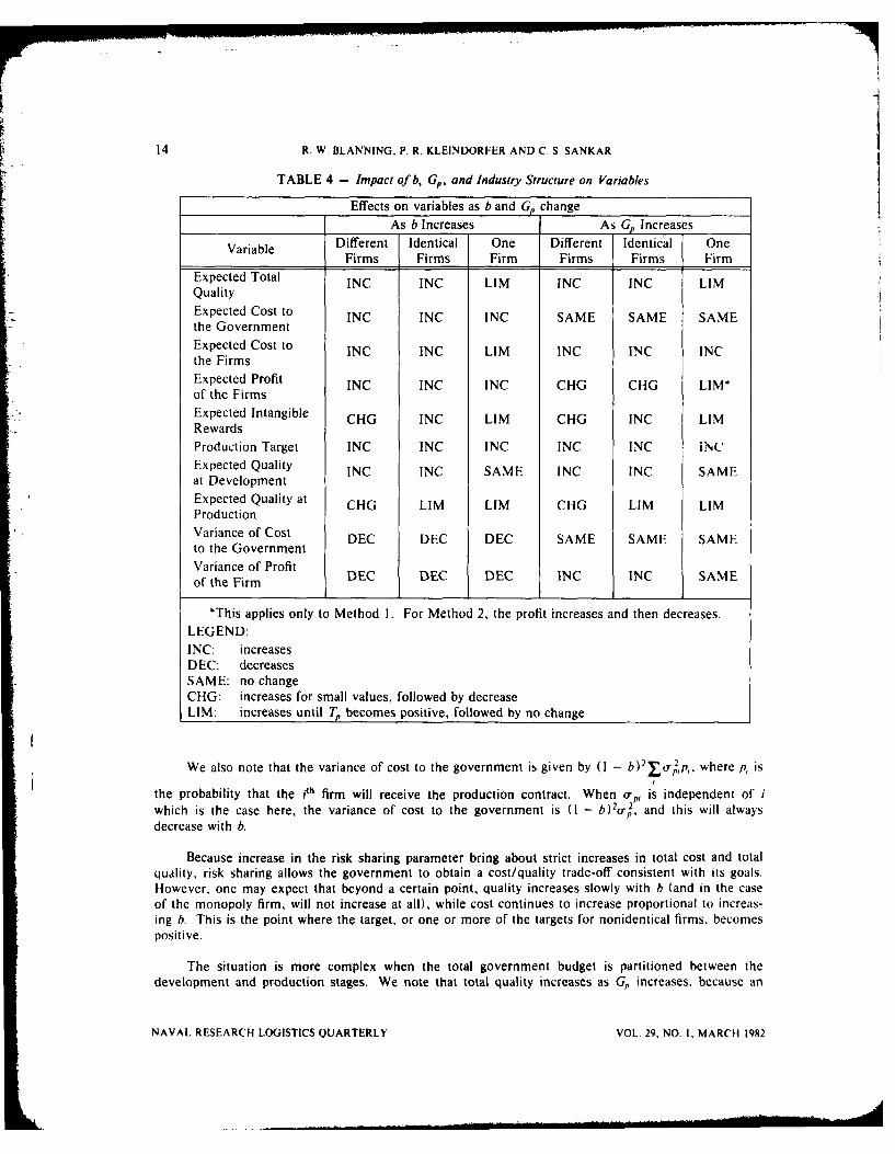
TABLE 4 - Impact of b, G., and Industry Structure on Variables
Effects on variables as b and G, change
As b Increases As G, Increases
Variable Different Identical One Different Identical OneFirms Firms Firm Firms Firms Firm
Expected Total INC INC LIM INC INC LIMQualityExpected Cost to INC INC INC SAME SAME SAMEthe Government
Expected Cost to INC INC LIM INC INC INCthe Firms
Expected Profit INC INC INC CHG CHG LIM*of the Firms
Expected Intangible CHG INC LIM CHG INC LIMRewardsProduction Target INC INC INC INC INC INC
Expected Quality INC INC SAME INC INC SAMEat Development
Expected Quality at CHG LIM LIM CHG LIM LIMProductionVariance of Cost DEC DEC DEC SAME SAME SAMEto the Government
Variance of Profitof the Firm DEC DEC DEC INC INC SAME
*This applies only to Method 1. For Method 2, the profit increases and then decreases.
LEGEND:
INC: increasesDEC: decreasesSAME: no changeCHG: increases for small values, followed by decreaseLIM: increases until T becomes positive, followed by no change
We also note that the variance of cost to the government is given by (I - b) 2 o,p,, where p, is
the probability that the ith firm will receive the production contract. When o', is independent of i
which is the case here, the variance of cost to the government is (I - b) 2o', and this will alwaysdecrease with b.
Because increase in the risk sharing parameter bring about strict increases in total cost and totalquality, risk sharing allows the government to obtain a cost/quality trade-off consistent with its goals.However, one may expect that beyond a certain point, quality increases slowly with b (and in the caseof the monopoly firm, will not increase at all), while cost continues to increase proportional to increas-ing b. This is the point where the target, or one or more of the targets for nonidentical firms, becomespositive.
The situation is more complex when the total government budget is partitioned between thedevelopment and production stages. We note that total quality increases as G, increases, because an
NAVAL RESEARCH LOGISTICS QUARTERLY VOL. 29, NO. I, MARCH 1982
DESIGN-TO-COST MULTISTAGE CONTRACTUAL INCENTIVES 15
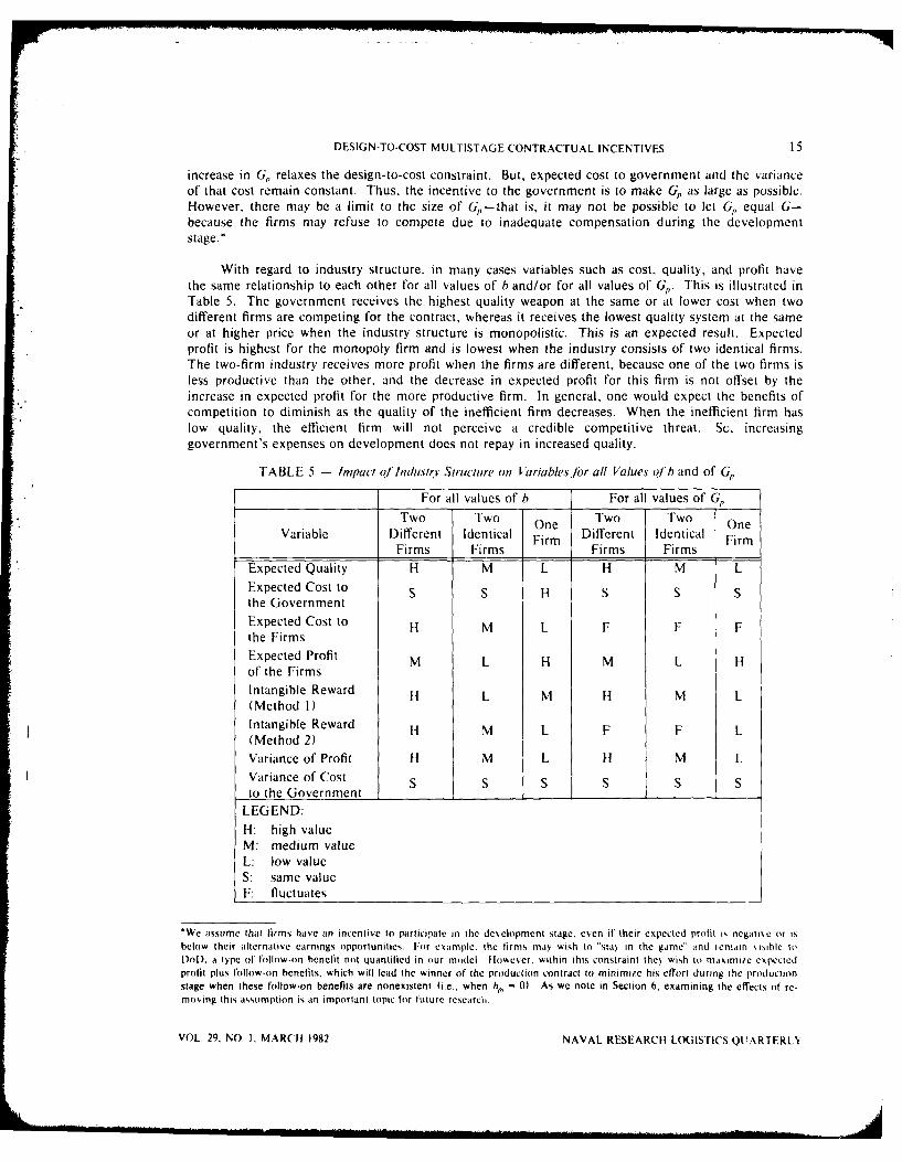
increase in G, relaxes the design-to-cost constraint. But, expected cost to government and the varianceof that cost remain constant. Thus, the incentive to the government is to make G, as large as possible.However, there may be a limit to the size of Gr-that is, it may not be possible to let G, equal G-because the firms may refuse to compete due to inadequate compensation during the developmentstage.*
With regard to industry structure, in many cases variables such as cost, quality, and profit havethe same relationship to each other for all values of b and/or for all values of G,. This is illustrated inTable 5. The government receives the highest quality weapon at the same or at lower cost when twodifferent firms are competing for the contract, whereas it receives the lowest quality system at the sameor at higher price when the industry structure is monopolistic. This is an expected result. Expectedprofit is highest for the monopoly firm and is lowest when the industry consists of two identical firms.The two-firm industry receives more profit when the firms are different, because one of the two firms isless productive than the other, and the decrease in expected profit for this firm is not offset by theincrease in expected profit for the more productive firm. In general, one would expect the benefits ofcompetition to diminish as the quality of the inefficient firm decreases. When the inefficient firm haslow quality, the efficient firm will not perceive a credible competitive threat. Sc, increasinggovernment's expenses on development does not repay in increased quality.
TABLE 5 - Impact qf Industry Structure on V/'ariables /br all Values of b and of GP
For all values of b For all values of G,
Two Two One Two Two OneVariable Different Identical Firm Different Identical Firm
Firms Firms Firms FirmsExpected Quality H M L H M L
Expected Cost to S S H S S Sthe GovernmentExpected Cost to H M L F F Fthe FirmsExpected Profit M L H M L Hof the FirmsIntangible Reward H L M H M L(Method I)Intangible Reward H M L F F L(Method 2)Variance of Profit H M L H1 M L
Variance of Cost S S S S S Sto the Government
LEGEND:H: high valueM: medium valueL: low valueS: same valueF: fluctuates
*We assume that firms have an incentive to participate in the development stage, even if their expected profit is negative or isbelow their alternative earnings opportunities. Fior example, the firms may wish to "stay in the game" and remain s i le toDoD, a type of follow-on benefit not quantified in our model lIok~ever, within this constraint they wish to maximite expectedprofit plus follow-on benefits, which will lead the winner of the production contract to minimie his effort during the productionstage when these follow-on benefits are nonexistent (i.e., when bt,, - 0) As we note in Section 6, examining the effects of re-moving this assumption is an important topic for future researci
VOL. 29, NO. I, MARCH 1982 NAVAL RESEARCH LOGISTICS QUARTERLY
16 R. W. BLANNING, P. R, KLEINDORFER AND C. S. SANKAR
The results described above are based on the assumptions that all firms in the industry will con#-pete for the production contract regardless of the expected profits and that the government will allow allfirms in the industry to compete (by paying a fixed cost for development) regardless of the productivityof the firm. These assumptions do not give rise to anomalies within the parameter ranges used here,contrary to expectation. For example, we observe that an increase in G, (and a corresponding decreasein the funds paid to the firms for their development efforts) results in an increase in quality with nochange in the expected cost to the government, and also results in an increase in expected cost to thefirms, regardless of industry structure. However, in reality, most firms have alternative uses for theirresources (current and fixed assets, experienced managers, skilled workers, etc.), and some of themmay decline to participate, once their expected profits do not compare favorably with those obtainableelsewhere. In fact, the existence of a negative constant term K,,(/,b) in (23) can result in negativeexpected profits for suitable contract parameter values. This will almost certainty cause a firm to with-draw from participation at the development stage.
Generally, the selection of government contract parameters (G,, -y, b, and a) must be compatiblewith the alternative earning opportunities of the firm. Such alternative market opportunities determinea set of contract parameters for each firm at which the firm would be willing to participate in thedevelopment effort and compete for the production contract. The government will desire a possiblydifferent set of values for the contract parameters, for which the cost is low, variance of cost is low andthe quality is high. The government must choose its values of Gp, y, b, and a from the set of contractparameter values which will guarantee prospective contractors earnings opportunities as attractive astheir alternative market opportunities.
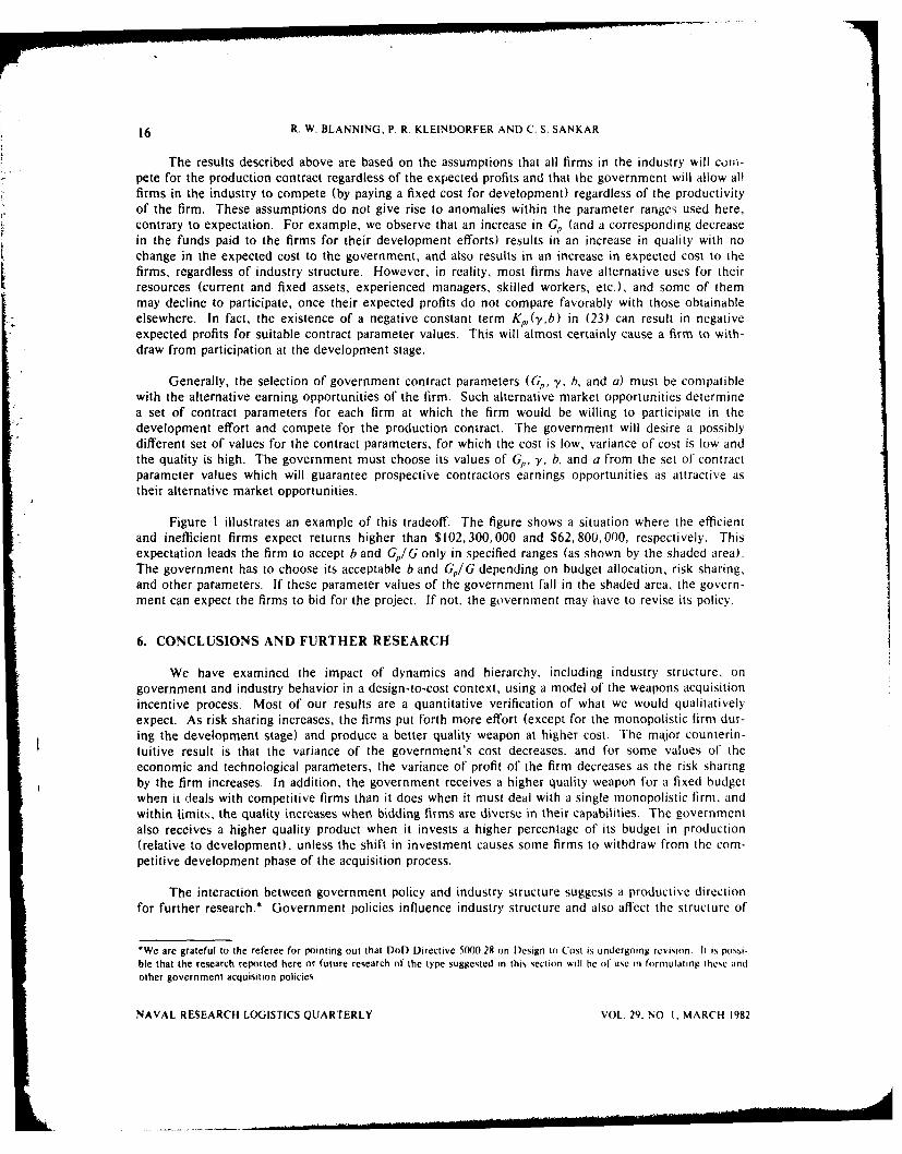
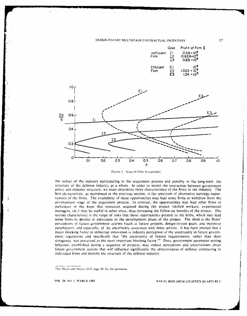
Figure 1 illustrates an example of this tradeoff. The figure shows a situation where the efficientand inefficient firms expect returns higher than $102,300,000 and $62,800,000, respectively. Thisexpectation leads the firm to accept b and Gp/G only in specified ranges (as shown by the shaded area).The government has to choose its acceptable b and GIG depending on budget allocation, risk sharing,and other parameters. If these parameter values of the government fall in the shaded area, the govern-ment can expect the firms to bid for the project. If not, the government may have to revise its policy.
6. CONCLUSIONS AND FURTHER RESEARCH
We have examined the impact of dynamics and hierarchy, including industry structure, ongovernment and industry behavior in a design-to-cost context, using a model of the weapons acquisitionincentive process. Most of our results are a quantitative verification of what we would qualitativelyexpect. As risk sharing increases, the firms put forth more effort (except for the monopolistic firm dur-ing the development stage) and produce a better quality weapon at higher cost. The major counterin-tuitive result is that the variance of the government's cost decreases, and for some values of theeconomic and technological parameters, the variance of profit of the firm decreases as the risk sharingby the firm increases. In addition, the government receives a higher quality weapon for a fixed budgetwhen it deals with competitive firms than it does when it must deal with a single monopolistic firm, andwithin limits, the quality increases when bidding firms are diverse in their capabilities. The governmentalso receives a higher quality product when it invests a higher percentage of its budget in production(relative to development), unless the shift in investment causes some firms to withdraw from the com-petitive development phase of the acquisition process.
The interaction between government policy and industry structure suggests a productive directionfor further research.* Government policies influence industry structure and also affect the structure of
*We are grateful to the referee for pointing out that Dot) Directive 5000.28 on Design to Cost is undergoing revision. It is possi-ble that the research reported here or future research of the type suggested in this section will he of use in formulating these andother government acquisition policies
NAVAL RESEARCH LOGISTICS QUARTERLY VOL. 29, NO. 1, MARCH 1982
IDESIGN-TO-COST MULTISTAGE CONTRACTUAL INCENTIVES 17
Case Profit of Firm $Inefficient II 059,108Firm .2 0.628-108
13 0.65 -108
Efficient E J08
Firm E2 1.023 - 108E3 1.04 -108
E I
08-
G Ip 0.6-
0.4-
0.1 0.2 03 0.4 0.5 06 07 08 09 10b
FiGuRE I. Arcas of Firm Acceplahility
the subset of the industry participating in the acquisition process and possibly in the long-term, thestructure of the defense industry as a whole. In order to model the interaction between governmentpolicy and industry structure, we must determine three characteristics of the firms in the industry. Thefirst characteristic, as mentioned in the previous section, is the spectrum of alternative earnings oppor-tunities of the firms. The availability of these opportunities may lead some firms to withdraw from thedevelopment slage of the acquisition process. In contrast, the opportunities may lead other firms toparticipate in the hope that resources acquired during the project (skilled workers, experienced
managers, etc.) may be useful in other areas, thus increasing the follow-on benefits of the project. Thesecond characteristic is the range of risks that these opportunities present to the firms, which may leadsome firms to decline to participate in the development phase of the project. The third is the firms'perceptions of future government actions (such as future projects, design-to-cost goals, and incentiveparameters), and especially, of ihe uncertainty associated with these acticns. It has been posited that amajor blocking factor in industrial innovation is industry perception of the uncertainty in future govern-
ment regulations and specifically that "the uncertainty of federal requirements, rather than theirstringency, Aas perceived as the most important blocking factor,"* Thus, government parameter settingbehavior, established during a sequence of projects, may induce perceptions and uncertainties aboutfuture government actions that will influence significantly the attractiveness of defense contracting toindividual firms and thereby the struclure of the defense industry.
*See %f.ers and Sce/ 11 I.1. page 29. for ihe quolanion.
VOL. 29, NO I, M,%RCI{ 1982 NAVAL RESUARCH LOGISTtCS QUARTLRLY
j

18 R. W. BLANNING, P. R. KLEINDORFER AND C S SANKAR
ACKNOWLEDGMENT
The authors gratefully acknowledge the helpful comments of Marvin Denicoff ol the Office ofNaval Research (ONR) on an earlier draft of this paper. This research was carried out under ContractN00014-77-C-071 of ONR.
REFERENCES
IlI "Application of Design-to-Cost Concept to Major Weapon Systems Acquisitions," Report to theCongress by the Comptroller General of the United States, U.S. General Accounting Office,Washington, D.C., June 23, 1975.
(21 Bonin, J.P., "On the Design of Managerial Incentive Structures in a Decentralized PlanningEnvironment," The American Economic Review, 66, 4, 682-687 (September 1976).
[3] Canes, M.E., "The Simple Economics of Inventive Contracting: Note," The American EconomicReview, 65, 3, 478-483 (June 1975).
[41 Cummins, M.T., "Incentive Contracting for National Defense: A Problem of Optimal Risk Shar-ing," The Bell Journal of Economics, 8, 1, 168-185 (Spring 1977).
[51 Defense Management Journal, "Design to Cost," Special Issue, 10, 4. 1-40 (September 1974).[6] Groves, T., "Incentives in Teams," Econometrica, 414, 617-631 (1973).[7] Groves, T., "Information Incentives and the Internalization of Production Externalities," in Theory
and Measurement of Economic Externalities, S. Lin, Editor (The Academic Press, New York,1976).
[81 Harris, M. and A. Raiv, "Some Results on Incentive Contracts with Applications to Education andEmployment, Health Insurance, and Law Enforcement," The American Economic Review, 68,1, 20-30 (March 1978).
[9] Jennergren, P.L., "On the Design of Incentives in Business Firms-A Survey of Some Research,"Management Science, 26 2, 180-201 (1980).
[10] Kleindorfer, P.R. and M.R., Sertel, "Profit-Maximizing Design of Enterprises through Incentives,"Journal of Economic Theory, 20, 3, 318-339 (June 1979).
[II] McCall, J.J., "The Simple Economics of Incentive Contracting," The American Economic Review,60, 5, 837-846 (December 1970).
[121 McCullough, D.J., "Design to Cost Problem Definition, Survey of Potential Actors and Observa-tions on Limitations," Paper P-928, Institute of Defense Analysis, Washington, D.C., January1973.
[131 Myers, S. and E.E. Sweezy, "Why Innovations Falter and Fail: A Study of 200 Cases," Report R75-04, Denver Research Institute, University of Denver, January, 1976.
[14] Office of Management and Budget. Circular A-109, April, 1976.[15] Ross, S.A., "On the Economic Theory of Agency and the Principle of Similarity," in Essays on
Economic Behavior under Uncertainty M. Balch, D. McFadden, and S. Wu, Editors (North Hol-land, Amsterdam, 1974).
[161 Tashjian, M.T., "Implementation of the Design-to-Cost Concept from the Contractual Point ofView," Defense Management Journal, 10, 4, 8-17 (September 1974).
NAVAL RESEARCH LOGISTICS QUARTERLY VOL. 29. NO. t, MARCH 1982
OPTIMAL STRATEGIES IN A GAME OF ECONOMIC SURVIVAL
Karl Borch
Norwegian School of BusinessBergen-Sandviken, Norway
ABSTRACT
The games of economic survival introduced by Shubik and Thompson seemtailor-made for the analysis of some problems in insurance and have foundmany applications in this industry. The optimal strategy in such games may bea so-called "band strategy." This result seems counter-intuitive and has causedsome puzzlement. This paper gives sufficient conditions so that the optimalstrategy will be of a simpler form, and it is argued that these conditions aresatisfied in most applications to insurance.
INTRODUCTION
The term "economic survival game" is really another name for the classic problem of' thegambler's ruin which can be traced back to Pascal. The new term is usually associated with Shubik andThompson [11], who extended some of the classic results to games of strategy. This generalization initself may not have been particularly fruitful, but it led to an increased interest in the multi-periodone-person game against nature. It is the starting point of the papers by Miyasawa 17] and Morrill [9],and the general ideas are behind the book by Dubins and Savage 141. A few years earlier De Finett; [31presented a similar model, as a generalization of the older actuarial theories, based on the probabiltthat an insurance company shall become insolvent or "ruined."
Miyasawa and Morrill both show that the optimal strategy can be a "band strategy" -a concept tobe explained in the next section. Strategies of this form are not intuitively appealing and do not seemto agree well with observations when the model is applied to situations in real life, but they have beenstudied for their mathematical interest by several authors including Hallin [6]. The purpose of this noteis to show that a band strategy can be optimal only in fairly exceptional cases.
The presentation is given in terms of insurance, which was the application Morrill 18] originallyhad in mind. This interpretation was also the starting point of De Finetti, and his models have beendeveloped and discussed extensively in actuarial literature, by, among others, Borch [I], Bihlmann 121
and Pentik~iinen [101. It is, of course, possible to give other interpretations to the model.
THE PROBLEM
De Finetti's starting point is an insurance company which underwrites identical portfolios in eachconsecutive operating period. Let the portfolio be characterized by:
P = premiums received in an operating period.
x = claims paid during the period, a stochastic variable with the distribution F(t.
VOL. 29, NO. 1, MARCH 1982 19 NAVAL RESEARCH LOGIlSI'S QI'ARII RI N
20 K. BORCH
Let So be the company's equity capital or "surplus" at the end of period t. Clearly, So follmx a randomwalk defined by:
S,+o= S, + P- X.
In insurance it is natural to assume that if S, < 0 the company is ruined and is not :ralkAed tooperate in the following periods.
At the end of period t, the company may consider paying a dividend, s, E (0. S,). he problem isthen to find the optimal dividend policy. De Finetti studied different assumptions about the cormrpan. ",objectives. One of these was that the company would seek to maximize the expected discouitled sumof the dividend payments:
(1) E{ V'srJ
where v E (0.1) is the discount factor.
Let V(S) denote the maximum, i.e., the expected discounted sum of the dividend payments itthe initial equity capital is S and if the company follows an optimal dividend policy. It is easy to seethat V(S) must satisfy the functional equation:
(2) V(S)= max s+v V(S- s + P- x)dF(x).0<s<S f
Essentially, early dividend payments are preferred, but a high dividend implies a low retainedsurplus and hence a high probability of ruin, i.e., that the payments will terminate. One would there-fore expect that an optimal s exists for any value of S.
Equation (2) can be solved by standard methods of dynamic programming, and Miyasawa andMorrill have shown that the optimal dividend policy is of the form:
s=0 for S < Z,
s=S- Z1 for Z < S <Z2
s=0 for Z 2 < S Z 3
S S - Z 2,+1 for Z 2,+ < S.
A policy of this form defined by a set of 2n + 1 numbers, is called a "band strateg)" by \Morrill.The special case with n = 0 he calls a "barrier strategy."
A band strategy implies that a company may omit or reduce its dividend after a successful operat-ing period, and this seems to be contradicted by the business behavior one can observe. The harrierstrategy does not invite the same objections. Essentially, it implies that the company decides that it isoptimal to maintain a certain equity capital Z. No dividend is paid if the equity capital is below thislevel. If the equity capital exceeds Z, the excess is paid out as dividend immediately. This seems rea-sonable and suggests that, in normal cases, a barrier strategy may be optimal.
Assume now that the company decides to adopt a barrier strategy defined by a number /. notnecessarily optimal. The expected discounted value of the dividend payments under this policy is
NAVAl. RESFAR(tH LOGISTICS QUARTERLY Vol 2Q, Ni) I. \1 \R('1 1142
STRATEGIES IN ECONOMIC SURVIVAL GAME 21
S+P(3) V(S, Z) = v fo V(S + P - x, Z) dF(x).
If a density, f(x) = F'(x), exists, this is an integral equation with the boundary conditions
V(S, Z)= OforS < Oand V(S Z)= S- Z + V(Z, Z) for S > Z.
The equation has a unique continuous solution for any nonnegative value of Z. Morrill's resultimplies that the solutions in Z to the equation
(4) a V(S, Z) -0aZ
are independent of S. A barrier strategy will be optimal only if (4) has a unique root in Z.
A SOLUTION OF THE PROBLEM
The integral equation (3) can be solved, and it is possible to study the roots of (4) by this directapproach. It seems, however, more convenient to take a roundabout way and consider a rather naivedividend policy. Assume that at the end of a profitable operating period the company pays the wholeprofit out as dividend immediately. If the period has given a loss, no dividend is paid.
Let W(S) be the expected discounted sum of the dividends paid under this policy when thecompany's initial capital is S: The function W(S) is clearly a solution of the integral equation:
(5) W(S) =f(P-x)f(x)dx+v W(S) f f(.x)dx+ vf W(S+P-x)f(x)dx
which evidently is far simpler than the functional equation (2). Setting the first term on the right-handside in (5) equal to C, and rearranging the other terms, the equation takes the form
(6) (1-vF(P)W(S)= C+vs W(S-x)f(x+P)dx.
Taking the Laplace transform of (6) one finds:
lvF(P)j f W(S)e-lsdS -- ! ~+ Iv W (x)e-dxJ1 JIf(,f(x+IPMedj
Writing
I - vF(P) = K
and
fo Jf(x+P)e-tdx = (t)
the equation takes the form
(7) if W(x)e--dx CK - vo (t)'
The left-hand side of (7) can be written
t - W(x)e--dx = W(O) + W'(x)e- dx.
As v() < 40) = I - F(P) < 1 - vF(P) = K for v < 1, it follows that the right-hand side of(7) can be expanded in a convergent series. Hence:
VOL. 29, NO. I, MARCH 1982 NAVAL RESEARCH LOGISTICS QUART-RI.')

22 K. BORCH
(8) W'(x)e-'dx + W(0) = -! J- (t)J.
By taking S = 0 in (6) one sees that W(0) = -, so that (8) can be writtenK'
(9) W'(x)e- dx = W(0) 0 I (t)J•
(0t)) is the Laplace transform of the nth convolution of f(x +p) with itself, which will be denotedby f/(x). Hence, f,(x)=f 0 f,-l(y)f(x+P-y)dy for n > 1, and let by definitionfJ(x) = f(x + P).
Taking the inverse transform of (9), one obtains:
(10) W'(x) = W(0) K fn(X).
From (10) W(x) itself can be found by integration:
W(x) = w(0) I i1 FI(x).
This result can be verified directly. To show this, introduce a distribution G (x) defined as fol-
lows:
G(0) = F(P)
G(x)=j x+P) for x>0.
Substitution of this in the calculations above gives
W(x) = C(I+ vG(x) + v2 G 2(x) ... I.
G,(x) is the probability that accumulated losses in n periods shall not exceed the initial equitycapital x. If this event occurs, the expected discounted value of the next dividend payment is vIC.
The convolutions G,(x) have a complicated form, and this symbol will not be used in the follow-ing.
The expansion (10) is, as noted, convergent, and W(x) as a discounted sum of distribution func-tions is a bounded and nondecreasing function of x. From (6) it follows that
W(0) C1 - vr(P)
Further, it is easy to see without any calculation, that
-PW(- = = V, (P - x)f W dx.
I o - v ,-o
The equation says that if the equity capital is infinite, the company will never be ruined, and theexpected dividend will be equal to expected profit in all future periods.
NAVAL RESEARCH LOGISTICS QUARTERLY VOL. 29, NO. 1, MARCH 1982

STRATEGIES IN ECONOMIC SURVIVAL GAME 23
From (10) it follows that
K
and
W'(oo) = 0.
A SUFFICIENT CONDITION THAT A BARRIER STRATEGY IS OPTIMAL
Consider now the equation
(11) W'(Z) = I.
It can be shown that the solutions of (4) and (1I) coincide. This is a tedious procedure, and onecan arrive at the result by an indirect approach.
If Z is a solution of (11) and if the company's capital at the end of an operating period is Z + zwith z > 0, we will have, at least for z, sufficiently small
W(Z + z) < W(Z) + Z.
Hence, the expected discounted sum of the dividends paid will increase if the company departsfrom its naive policy and immediately pays the amount z out as dividend.
Similarly, if the capital is smaller than Z, it will be optimal to retain profits until the capital hasbeen brought up to Z before paying any dividend.
A sufficient condition that equation (11) has a unique root is W'(0) > I and W'(x) < 0.
Differentiation of (10) gives
(12) W "(X) W (0) (A)
n=l
From the definition of the convolution, it follows that:
fW(x) f 1 ()f(x+P-y)dy for n 2.
Differentiation of this expression gives:
f,(x) f(P).f,_1 (x) + f,-i(y)f(x+P-y)dy
and by definition
f(x) f'(x+P).
Substitution of these expressions int6 (12) gives
(13) W"(x) = W(0) K f'(x + P) + -- f(P)f(x + P)
+ W(0) ( f,' O'). (x+P-Y)v +-vfftP)+,(P).
VOL. 29. NO 1. MARCH 1982 NAVAL RESEARCH LOGISTICS QUARTERLY

24 K. BORCH
The first term in (13) is negative if
(14) f'(x+ P) + -- f(P)f(x + P) < 0.K
Substitution of
.f'(x+P- Y) - .f(P)f(x+ P-y)
in the following terms, shows that they all vanish. Hence, (14) is a sufficient condition thatW"(x) < 0.
Condition (14) can be written:
f'(x + P) vf(x + P) K f(P)
and this gives
I/(x+P) < f(P)e K f(p)X.
Hence, equation (II) will have a unique root if the claim density goes to zero at least as rapidly asan exponential.
.\ necessary, but not sufficient condition is that f'(x + P) < 0 for x > 0. For a unimodal distri-bution this condition will be satisfied when P is greater than the mode. The typical claim distribution ininsurance will be skew, with a long tail. For such distributions the mean will be greater than the mode,and the premium P will again normally be greater than the mean, i.e., than expected claim payments.
If the necessary condition is satisfied, the sufficient condition (14) appears as a mild regularitycondition for the tail of the distribution, and the curious cases found by Miyasawa and Morrill may bedismissed as interesting but not very relevant.
Clearly, the company will not find it optimal to maintain positive reserves unless
W'(0) > 1.
Substitution of the expressions derived from (10) gives the condition in the form:
vf(P) fP (P - x)f(x) dx > (1- vF(P)) 2 .
Since the left-hand side will go to zero with P, it follows that the premium must be above a cer-tain level to induce the company to risk any part of its equity capital as reserves in the underwritingbusiness. The company will, however, not refuse to underwrite any portfolio, since it cannot loseunless it put some of its own money at risk.
SPECIAL CASE
As a simple special case assume that the claim density is exponential, i.e.,
/( ) = e -.
N .\. AL RI.SARCII LOGISTICS QUARTERLY VOL. 29. NO. I, MARCH 1982
. . . . . . . ... . . .. .. . . . . . . ... . .. ----
STRATEGIES IN ECONOMIC SURVIVAL GAME 25
Substitution in the general formula gives:
W -- l-v+ve-P l-v+ve P
and
W'(x) = e e xp I - -- veX
It is easy to see that W"(x) < 0, and hence that a barrier strategy is optimal.
Equation ( 1) which determines the optimal strategy takes the form
Z = InC + lnv- P- 2 1n(1-v+ve-P),I - v+ ve -
or by substituting the expression for C and writing v = (1 + i,
- In (P-I +e -P) - 21n (I + i) - P - 21n (+e-).i +e- P
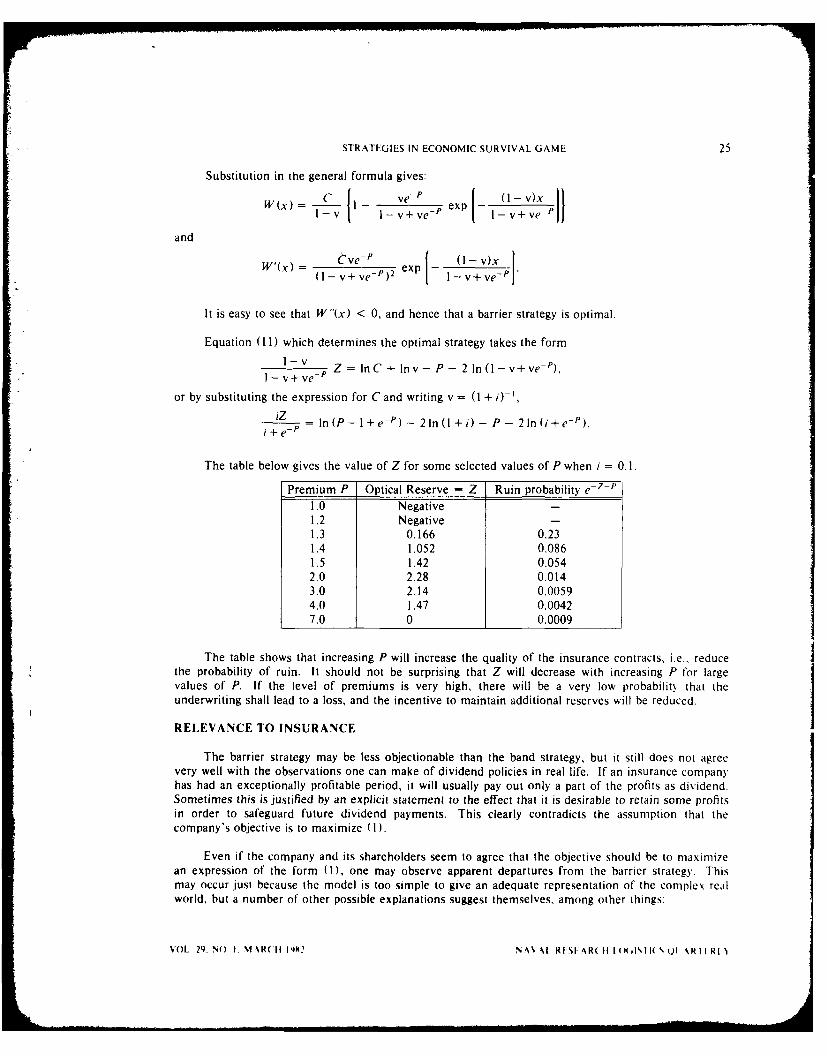
The table below gives the value of Z for some selected values of P when i = 0.1.
Premium P Optical Reserve = Z Ruin probability e- Z -P
1.0 Negative1.2 Negative -1.3 0.166 0.231.4 1.052 0.0861.5 1.42 0.0542.0 2.28 0.0143.0 2.14 0.00594.0 1.47 0.00427.0 0 0.0009
The table shows that increasing P will increase the quality of the insurance contracts, i.e., reducethe probability of ruin. It should not be surprising that Z will decrease with increasing P for largevalues of P. If the level of premiums is very high, there will be a very low probability that theunderwriting shall lead to a loss, and the incentive to maintain additional reserves will be reduced.
RELEVANCE TO INSURANCE
The barrier strategy may be less objectionable than the band strategy, but it still does not agreevery well with the observations one can make of dividend policies in real life. If an insurance companyhas had an exceptionally profitable period, it will usually pay out only a part of the profits as dividend.Sometimes this is justified by an explicit statement to the effect that it is desirable to retain some profitsin order to safeguard future dividend payments. This clearly contradicts the assumption that thecompany's objective is to maximize ( I ).
Even if the company and its shareholders seem to agree that the objective should be to maximizean expression of the form (I), one may observe apparent departures from the barrier strategy. Thismay occur just because the model is too simple to give an adequate representation of the complex realworld, but a number of other possible explanations suggest themselves, among other things:
VOL 29. No t. MiR(II IX NV.\%M RESFAR(t 11 t(KilSIl( ,Q1 *RII RI
26 K. BORCH
(i) It may be considered fair that the insured, i.e., the policyholders, should receive somebenefits after a very profitable period. One way of arranging this would be to increase the company'sreserves, and thus reduce the probability of ruin in the next period, i.e., improve the security of thepolicy holders. In some countries the governments seem to try to induce insurance companies to takethis attitude and maintain a conservative dividend policy.
(ii) The managers of an insurance company may rightly or wrongly believe that they will beblamed for sharp reductions in dividend payments. Their natural reaction may then be to argue in
favor of a conservative dividend policy which, incidentally, will increase the expected life of the com-pany and, hence, the job security of managers and other employees.
One will get a smoother sequence of dividend payments by assuming that the company's objectiveis to maximize
(15) v'- (s,)t=0
where u(s) is a concave utility function.
This generalization of De Finetti's model has been studied by several authors, by, among others,Hlakansson [5], who finds that, for a particular class of utility functions, the optimal strategy is of theform s = qS. This means that at the end of each operating period the company pays out a fraction, q,of its equity capital as dividend, and represents behavior in conformance with observations. The objec-tions to criterion function (15) are essentially of a theoretical nature. If the company should reduce thescale of its operations, or stop selling insurance altogether, it would find it optimal to pay out its equitycapital in an infinite decreasing sequence. This might make sense in the consumption plans discussedby Hakansson but not for a dividend policy.
The discount factor v which appears in the formula, should be based on an interest rate whichrepresents a pure risk premium. The company's reserves can be invested to earn a return, which couldbe paid directly to the shareholders as owners of the capital. Theoretically, they could even keep thecapital, provided that they accept liability for possible losses in the insurance operations. Governmentregulations will usually require that the reserves should be kept in low-risk assets, which also must be
of fairly liquid nature, since the reserves can be called upon at short notice to pay claims. This meansthat the rate of return on the reserves will be modest, probably close to the risk-free market rate ofinterest. The shareholders risk their capital as reserves in the insurance company and will require ahigher expected return. This interest differential seems to be the one to use for determining thediscount factor.
REFERENCES
(11 Borch, K., The Mathematical Theory of Insurance (D.C. Heath & Co., Lexington, MA, 1974).[21 BUhlmann, H., Mathematical Methods of Risk Theory (Springer Verlag, Berlin, 1970).[31 De Finetti, B., "Su una Impostazione Alternativa della Teoria Collettiva del Rischio," Transactions
of the XV International Congress of Actuaries, 2, 433-443 (1957).(41 Dubins, L.E. and L.J. Savage, How to Gamble ff You Must (McGraw-Hill, New York, 1965).[5] Hakansson, N., "Optimal Investment and Consumption Strategies under Risk for a Class of Utility
Functions," Econometrica, 587-607 (1970).[61 ltallin, M., "Band Strategies: The Random Walk of Reserves," Blatier der DGVM, 14, 231-236
(1979).[7] Miyasawa, K., "An Economic Survival Game," Journal of the Operations Research Society of
Japan, 95-113 (1962),[81 Morrill, J., "Discrete Economic Survival Game Models for Insurance Surplus Distribution,"
Unpublished dissertation, University of Michigan, Ann Arbor, MI, 1964.
NAVAL RESEARCH LO(ISTICS QUARTFRLY VOL 29. NO. t. MARCH 1982
STRATEGIES IN ECONOMIC SURVIVAL GAME 27
[91 Morrill, J., "One-Person Games of Economic Survival," Naval Research Logistics Quarterly, 49-69(1966).
1101 Pentikiinen, T., "A Model of Stochastic-Dynamic Prognosis: An Application of Risk Theory toBusiness Planning." Scandinavian Actuarial Journal, 29-53 (1975).
1111 Shubik, M. and G.L. Thompson, "Games of Economic Survival," Naval Research Logistics Quar-terly, 111-123 (1959).
VOL. 29, NO. I, MARCH 1982 NAVAL RESEARCH LOGISTICS QUARTERLY
DIAGNOSTIC ANALYSIS OF INVENTORY SYSTEMS:AN OPTIMIZATION APPROACH*
Gabriel R. Bitran, Arnoldo C. Hax and Josep Valor-Sabatier
Sloan School of ManagementMassachusetts Institute of Technology
Cambridge, Massachusetts
ABSTRACT
The objective of a diagnostic analysis is to provide a measure of perfor-mance of an existing system and estimate the benefits of implementing a newone, if necessary. Firms expect diagnostic studies to be done promptly andinexpensively. Consequently, collection and manipulation of large quantities ofdata are prohibitive. In this paper we explore aggregate optimization models astools for diagnostic analysis of inventory systems. We concentrate on thedynamic lot size problem with a family of items sharing the same setup, and onthe management of perishable items. We provide upper and lower bounds onthe total cost to be expected from the implementation of appropriate systems.Howe.er, the major thrust of the paper is to illustrate an approach to analyzeinventory systems that could be expanded to cover a wide variety of applica-tions. A fundamental by-product of the proposed diagnostic methodology is toidentify the characteristics that items should share to be aggregated into a singlefamily.
I. INTRODUCTION
Inventory-control theory provides a wide variety of models to manage effectively products vithdifferent characteristics. Extensive surveys are available that culminate in a taxonomy identif.ingspecific decision rules to manage inventories under a number of conditions. (Silver [7]. Nahmias [51.and Aggarwal [1].) A very legitimate concern of many managers today is to understand the extent toskhich these models could contribute to the enhancement of the performance of their current inventorysy-stem. Consequently, management-science practitioners are frequently faced with requests to estimatethe benefits for improving the performance of such systems. Firms expect that the estimation processin itself will not represent a major project and consume a considerable amount of human and financialresources: the analysis must be reasonably accurate and inexpensive.
Iwo basic approaches have emerged to comply with those requirements. One, the statisticalapproiach, is based on analyzing the inventory performance on a relatively small sample of items andgenerating inferences that can be applied to the whole population. The other approach, based onoptimtzation techniques, consists in devising simple models to estimate the benefits of implementingthe proposed system.
lhe simplified models are derived by aggregating items into families, thereby reducing the datacollcLtion and computation efforts. The ultimate objective is the generation of bounds relating theaggregated model to the original problem. Zipkin [121 and Evans [3] have developed such bounds forliner ind tratsportation models, respectively.
'I - ir, h t, perforncd under Contract N00014-75-C-0556 for the Office of Naval Research
') 1 Ni A t.R( If 1982 29 NAVAL REiSFARCI( LO(IISTICS Qt ARII RI
MECDI0 PAGE B N-LNOT FlrLD
31) G. R. BITRAN, A. C. HAX AND J. VALOR-SABATIER
The management-science literature has rarely addressed the identification of problems and the a-priori measurement of benefits to be derived from the implementation of a proposed new system.Recently Hax, Majluf and Pendrock [4], and Wagner [9] have stressed the importance of developingdiagnostic analysis tools. In particular Hax, Majluf and Pendrock [4] report the results of a diagnosticania sis of a large logistics system.
In [21 we illustrated how statistically-based techniques, like clustering, inference and sampling,may be used in diagnostic studies. In this paper we focus on the application of aggregate-optimizationmodels. In Section 2 we concentrate on the dynamic-lot-size problem with a family of items sharingthe same setup. We examine an aggregation scheme and compute upper and lower bounds on the totalcost to be expected from the implementation of appropriate systems. We also provide conditions underwhich the solution to the aggregate problem solves the original problem. In Section three we analyzethe management of perishable items. An aggregate version of the newsboy problem is studied andbounds are determined. Conclusions and topics for future research are discussed in the last section.
We would like to emphasize that although this paper examines two classes of inventory models,our aim is to propose a general approach to design diagnostic methodologies that could be easilyextendable to a wide spectrum of optimization models. Moreover, we hope that the result of ouranalv sis not only contributes to the development of quantitative measures to evaluate inventory perfor-mance, but also provides insights into the conditions that have to be met by the items to become candi-dates for aggregation into a family unit. This last result could contribute to the important subject ofaggregate planning.
2. I.OT SIZE PROBLEMS: A DIAGNOSTIC ANALYSIS
In this section we develop diagnostic procedures to estimate ordering and inventory carrying costsassociated with the operation and management of a family of items replenished in lots. The objectiveof' this procedure is to obtain estimates of total costs while reducing as much as possible the massivemanipulation of data and the computational requirements. We derive error bounds for aggregate prob-lems and rules indicating how to aggregate the items in a family to minimize such errors.
We address practical situations in which all items in a family are replenished simultaneously andshare the same ordering costs.
Whenever the items in the family satisfy the conditions underlying the economic order quantitysystem [61, the total annual cost of ordering and holding the family in stock is easily shown to be
12.1) TC= 2Sr (Div,)
where .5, r, D, and v, are, respectively, the ordering costs, the inventory carrying factor, the annualdemand of item i, and the unit cost of item i. The cost of holding in stock one unit of product i forone year is rv,. Therefore, (2.1) can be rewritten as
TC = (production cost of family)"1 2 2r.
In this case total ordering and holding cost for the family of items can be readily computed fromaggregate data. However, when the assumptions underlying the economic order quantity system differsignificantly from the actual conditions, the estimation of the costs must be based on more complexmodels.
In what follows we assume that the demand for each item in the family, in each period 1. 2 . T",is deterministic. The inventory control problem then, is to solve the following mixed integer program-ming problem:
N\N\1 R1F.\R(II tOGI6STICSQUARTERLY VOL. 29, NO, 1, MARCH 1982
DIAGNOSTIC ANALYSIS OF INVENTORY SYSTEMS 31
(P) zp = min f(x) = S8 xu + p,,,, + h,,, (x,., - d,.,)
subject to
" (x,. - d,.) > 0 t 1 ,2. T 1,2. N.
i-I
xi., 01 1 2, T;i= 1.2 N.
N1, if ",. > 0
!8 N X .t = N, 0. if xi.,< 0
- i=1
t 1,2 ;..... Ti= 1,2. N.
where p,, h,, d,., x,., and S, are, respectively, the unit cost, holding cost, demand and amount orderedfor item i in period t, and the ordering cost in period t. Without loss of generality, we assume that theinitial inventory is zero.
We will compare problem (P) with the solution obtained from the following aggregate problem:
(AP) zAP = min P(y) = S18(yd) + py, + h, (Y, - d,)
subject to
S(y,-d,)> 0 t 1,2. T
y, >0 T =1, 2... T1, ifY, > 0
8(')= 0, if Y< 0 t =1,2 .... T
where p,, h,, d,, y, and S, are the unit cost, holding cost, the demand and amount ordered for the fam-ily in period t, and the ordering cost in period t. We assume that y, and d, are defined as follows forconveniently selected constants k, > 0, i = ,2 . N:
(2.2) ,= k,x,, i = 1, 2... .T, i= 1,2. N.
(2.3) d,= k,d,., I = 1,2. T, i= 1,2. N.
Therefore, if x,., i= ,2. N = 1,2,.. T is feasible in (P), y, = 1. 2. T definedas in (2.2), is feasible in (AP). Wagner and Whitin [101 provide an efficient dynamic programmingalgorithm to solve (P) and (AP).
VOL. 29, NO. I, MARCH 1982 NAVAL RESEARCH LOGISTICS QUARTERLY

32 G. R. BITRAN, A. C. |tAX AND J. VALOR-SABATIER
The expression below, for a pair (x, y0 satisfying (2.2) and (2.3), is useful in our development.
(2.4) 1(X) -0 p(,v S6{ xi -(v,)I
+ h (xv., - d,,,) - h, (y., - d.) + P,, 1 plY,+=1 1~ ~ =1 ' i1"
I=] i~lr lH j (h, -/,k,)(x,, - d, + x,.,(p, -, Apr)
The second equality follows from (2.2), (2.3) and the fact that
l8 X, 81~ =(v,) t = 1, 2,., T.
PROPOSITION 2.1 (Theorem 6 in [8]): (P) and (AP) have at least one optimal solution of theform
(2.5) ( v d,.)X,. = 0 1 = 1,2. T; i = 1,2. N
(2.6) ( d)y,+1 0t = 1.2. T.
Note that (2.5) and (2.6) characterize the extreme points in (P) and (AP), respectively. Theproposition indicates that in order to compare zp and ZAP, it is sufficient to consider feasible solutions of(P) and (AP) such that in each period, either the initial inventory is zero, and eventually an order isplaced, or the initial inventory is positive and no order is placed.
PROPOSITION 2.2: Let Y, 2 = , 2 .. T be feasible in (AP) and assume it satisfies (2.6).Then, there is a unique set x,., t = 1,2 ..... T, i = 1,2. N feasible in (P) such that v, and x,,
are related as in (2.2) and x,., satisfies (2.5).
Whenever x, and y, i = 1, 2 ... N, t = 1,2. T ar. as in Proposition 2.2 we will say thatthey are corresponding feasible extreme point solutions.
Unfortunately, ify, t = 1, 2 .... T is an optimal extreme point in (AP) the corresponding feasi-ble extreme point solution in (P) need not be optimal, in general, in that problem. In fact, it is noteven true, in general, that the optimal value of one of the problems is a lower or upper bound of theother. Two instances where a relation between Zp and ZAP is known a priori are given in the next tworesults.
PROPOSITION 2.3: If k,,p, and h, are chosen such that p, ,- prk, < 0, h., - hk, < 0(p,, - p,k, >_ 0, h,, - hlk, > 0) for all i and all t, it follows that
ZAP > :p (Z4p Zp).
PROOF: Follows by Proposition 2.2 and Expression (2.4). El
COROLLARY 2.1: Assume the unit and holding costs p,.,, h,.i = 1.2. N andt = 1,2 ... T remain in the same proportion for all i, i.e., pf., = k,p,. h,, = k,h, for some k, > 0,p, > 0 and h, > 0. Then, zp ZAP as long as p, and h, are used in (AP) as the underlying unit andholding costs.
NAVAL RESEARC11 LOGISTICS QUARTERLY VOL 29. NO 1, MARCH 1982
DIAGNOSTIC ANALYSIS OF INVENTORY SYSTEMS 33
PROOF: Follows by Proposition 2.3. 11.
A special case of Corollary 2.1, of interest in practical settings, is when the unit and holding costsare constant for each item over the planning horizon and the holding cost is proportional to the unitcost. In these situations pi., = p,h, = h, and h, = rpi for all items and therefore zp = zAP.
Even when the conditions of corollary 2.1 do not hold, we may prefer to solve (AP) instead of(P) either to save computational work or because family demand data is readily available or evenbecause family demand can be forecast with greater accuracy than item demand. k, and h, can alwaysbe chosen to satisfy the conditions in Proposition 2.3. However, the gap between zp and z.Ap can begreater than desired. In what follows we attempt to measure this aggregation gap under quite generalconditions.
In the remainder of this section we assume the following:
T N D1k,= 1, D,= Z d,,, D= Z Di, c =D
N N ND, = d,,, = c,D, + P,,, p, = cip,, and h, = h,
i~l /=1i-I
where, for all expressions
i=1,2. N, t = 1,2. T.
Note thatA T
(2.7) ., = ','- = 0
for all i and t.
Let x be feasible in (P) and let
W)= t : I< t < T "xi., > 0
For t E (x) we denote by n(x, t) the smallest integer in.(x) U {T + 1) larger than t, i.e.,
n(x, t) = min{r :r > t. r E R(x) U {t + 1}}.
M(x) and n (x, t) correspond, respectively, to the set of time periods when any production occursand the next such period after t.
Assume 3c is an optimal extreme point of (P). Then,
ZP TS NXU N I n( i0-I n(m.)-l T-I1
t-I I .- ~ -I I' k.! U
Let i be the corresponding feasible extreme point solution to 3 in (AP) then,
r N n(x.iI 1 "U.0- I 7i 1Z e = Y S , 8 ( -i) + 7 & , P .d,, + 7 d., h ,ut [-IL r-1 -r+l u-t I
o7 (x0 Inr)I n(x.t)-I -
= S,8(y,) + p,,(c,D, + ,P,.,) + Z (c,D, + P,,) h,,u
VOL 29. NO I, MARCII 1982 NAVAL RESEARCH LOGISTICS QUARTERLY
34 G R. BITRAN, A. C IAX AND J VALOR-SABATIER
= " (T) + I ID D, p, + 'I
) -pD, + )"'-1+1 U-1
+ P., V',., + 'P,, + h,.u zAp + q(.)1( U-Ii r1 U
where(2.8) 1(1 ) = J p,., ,. + , p,., + 1h,. •
E 'i(x) 1=1 7t+I ui1
We have just proved
PROPOSITION 2.4: lfk is an optimal extreme point of (P),
Zp > ZAP + ZAP).
Similarly, define for any extreme point y in (AP)
,q(y) = (t:l I< t < T, y, > 01
and
n(y, t)= min{:r > t, t E M (y) U {T+ 1).
Let F be an optimal extreme point of (AP) and k be its corresponding feasible extreme point solutionin (P). Then,
ZAP = y p,D, + Dp+ = SIi .j,.,
+ 1 p8 .(d,, - P,) + IP:, + hi (d,. - ) z - l
t .( )i=1 r-t+l U-1
where
(2.9) I'(y) = pu0., + I pI + h,.II.,E'..W '¢y I t= r+l i JU=1
Consequently,
PROPOSITION 2.5: lf3F is an optimal extreme point of (AP),
zP - ZAP + Z (A).
COROLLARY 2.2: If y and 3 are optimal extreme point solutions of (AP) and (P), respectively,then
'¢(x) < Zp - ZAP < I').
Note that i and Y need not be corresponding feasible solutions in Corollary 2.2.
NAVAL RESEARCH LOGISTICS QUARTERLY VOL. 29, NO. I, MARCH 1982
DIAGNOSTIC ANALYSIS OF INVENTORY SYSTEMS 35
Corollary 2.1 shows that if the unit and holding costs, for each item in the family, remain in theA'
same proportion, then Zp = ZAp. A similar result holds for the demands even when h, .; C, hl.r
Nand/or p, e cp,,.
COROLLARY 2.3: Assume that tP, = 0 i = 1,2. N, = 1,2. T, that is, d,., c.D,.Then
Zp = ZAP.
PROOF: From (2.8) and (2.9) we have 4()60 = F ) = 0 and by Corollary 2.1,O < Zp - ZAp < O. Hence, zp=zAp. l
Corollary 2.3 provides an interesting interpretation of problem (AP). More specifically, it shows
that solving the aggregate problem is equivalent to solving the detailed problem with the demands d,
replaced by ciD, -e- D,. In fact, under the conditions of the corollary, the following stronger result
holds:
PROPOSITION 2.6: Under the conditions of Corollary 2.3, f(x) = '(y) for every pair x. y ofcorresponding extreme points.
PROOF: Note that,(x) EP(y) and n(x, ) = n(y, t) for allt iE(x) andR(y).
s(x) s '8 , + _ Ip,.,d, + i(h,.,+P p,,d .lI 9P (X) U PH I ll~
S' (V, + i +p.,cD1=1 i-I t C.A(y) 7-1+l i u=1
-,,8,') + .pr Dt + hu + p, D, =P(v).t-1 t E ' ) I t1+l tu=t I I =
We should note here that the conditions of Corollary 2.3 (proportionality of the demands) areequivalent to requiring the multiplicative seasonal factors of the different items to be equal period byperiod. In what follows we prove this result.
PROPOSITION 2.7: Assume that we fit the model d, = s,.,(boo, + bl.1 t) to every item i, whereb0.j and b1 , are determined by the least squares method, and the s., are the multiplicative seasonal fac-tors defined according to Winters [111. Then, if the demands are proportional as required in Corollary2.3, it follows that s,, = s., for all i = 1, 2 ... N, / = 1,2 ..... L and t = 1,2. T.
PROOF: For each of the N items the offset value b0, and the linear trend b., have the propertyof minimizing the sum of squares of the seasonal variation:
d,- (t- )T-
b( = A (Tdi, - D) (t - t)(70- 0)1 1-1t--li
bo.,= T -. , I
VOL. 29, NO. 1, MARCH 1982 NAVAL RESEARCH LOGISTICS QUARTERLY
36 G. R. BITRAN, A. C. IIAX AND 3 VALOR-SABATIER
whereT -
A , 1 an d t = + TT 2
the seasonal factors ared,~
si -I bo, + tbl.i
Assuming proportional demands: d,., = k.ld1,, i = 1, 2. N t= 1, 2. T for a generic item i
and a fixed "base" item 1, we get
d , ki.(bo. + tb.,)st = s.,(k,..b 0, + tk,1.b.,
butr r
bl. =A I (Td,, - D,)(t - t) = A , (Tk,.,d., - k,.1Dl)(t - t)
Tk,,tA d (d,, - DI) (t - ) =k,,tb,.,
I- 1
and
D - k,,1D k = kbo.boa = -, - b 1. - - kb
Therefore,
d, s.,(bo., + tbl,)
which implies:
s, si., i= 1,2. N t= 1,2. T.
When the conditions of Corollary 2.3 do not hold it is possible to derive bounds for the gapbetween zp and zAp as we show in the following development.
Let a, be defined as the maximum absolute value of the relative difference between each perioddemand of product i and its annual demand, and the corresponding ratio of the family, i.e.,
d, D,D, D
(2.10) a,- max i= 1,2. N.1-1.2.....r di.,ud,,>0 D ,
Hence,
c,D, d, - O.l(2.11) a,= max - = max I
1 .2,...,T d , -I.2..., dT,= d,, > d:d,.>O
-- max--hw
,-I.2. .," rt
NAVAL RESEARCH LOGISTICS QUARTERLY VOL. 29. NO. 1. MARCH 1982

DIAGNOSTIC ANALYSIS OF INVENTORY SYSTEMS 37
Let
a= maxa,= max - = ,2, T 'di, > 0, i 1, 2,i-1,2....N ,=22...N N d,
Thus,
I<adi,, i =1,2. N, t= 1,2. T and di, > 0.
Note that when d,, - 0, .= -cD, 0.
For any extreme point x in (P),(2.12) 11(x)l= I , I". P.,.) I. I
A Pn(x,)-j , + n0,' h
[E 4() i I iT; P r = +l U=1
-4 (X)i1 ~ T=(+] U=17:d,.,>0 rd,., >0
N jn(xtf)- .,I 'P n(x.i) ] 'I< pip.-+ h,., ,
t 4 k j - -I+ , U=.t+d,> -:d,. >0
A' In(x,)-I nfx.,-I I-P,,, + I = a [Pp(x) + Hp(x)]
where Pp(x) and Hp(x) are the proportional purchasing and holding costs in problem (P) associatedwith the feasible point x.
Similarly, for any extreme point y in (AP)
(2.13) IF(y)I < a p,,d, , +I .t, v - - -t$-I uj
However,
d, - cO, < Id,., - cA = I ,I < ad,.,
Thus, if a < 1,
(2.14) di, , 1 c,D,.-a
Substituting (2.14) in (2.13)
(2.15) IF(y) I a In(P.0I N N n(v~h 1')l=. Z ,:o + Z h,,c,.
a E (yI 7 - 1-I -I T-r+l U-t
-- a [' AP(Y ) + H APWY I- a
where Pp(y) and HAp(y) are the proportional costs in (AP) corresponding toy.
VOL. 29, NO. I, MARCH 1982 NAVAL RESEARCH LOGISTICS QUARTERLY
38 G. R. BITRAN, A. C. HAX AND J. VALOR-SABATIER
Before deriving the desired bounds we observe that if i and 3 denote, respectively, optimalextreme points of (P) and (AP) then zp and ZAP can be written as
Zp = Sp( ) + Pp x) + Hp U)
and
ZAP = SAp( ) + PAP(y) + HAP(C)
where Sp(x) and SAp(Y) are the fixed costs associated with 5 and . Also, to use as reference value inthe measurement of the gap, we define
- [ S'+ pi., d,. + max(Pp(x) + Hp(x): x feasible in (P)} = S' + (p' + H)max
andT7-
-max = (S, + pD,) + max (PAP (v) + HAp(y):y feasible in (AP)) = Sy + (PY + HY)mx.
Therefore, by Proposition 2.5 and Expression (2.15), if a < 1
ZP-ZAP < IF_(y) I
ZMax - ZAP S' - SAP(Y) + (PY + HY)max - PAP(Y) - HAp(Y)
a HAp(Y) + PAP(Y)
-a Sy - SAp(.V) + (pv + HY)max - PAP() - HAP(U)
Since (Pv + HY)max > PAp(.U) + HAp(Y) > 0 and
Sy > ZAP = SAP(y) + PAP() + HAp(j)
it follows that
(2.16) Zp - ZAP a
4max ZAP
Expression (2.16) provides an upper bound on the gap between the optimal values zp and Z4prelative to zva, provided that a < 1. Another gap measurement often employed in this type of analysisis obtained considering only the aggregate problem as a basis for comparison, i.e.,
aI [P4p(..() + H4p(3)](2.17) zp- ZAP IF( I -a a
Z4p ZAP SAP() + PAP(V) + H 4p(y) 1 - a
Other upper bounds can be obtained as follows:
(2.18) ZAP - Zp -(b) C a[Pp(x) + Hp()<Z4ax - ZAP SX + (Px + HX)max - SP(O) - PP(-i) - Hp(iM) Sx - Sp(T).
The inequalities in (2.18) are implied by Proposition 2.4, Expression (2.12) and the facts that(PI + H*)m > Pp(C) + Hp(i) >, 0 and S'- S,(3) > Pp(3c) + Hp().
Similarly,ZAP- zp -3(j-) (a
(2.19) < -( 60Zp Sp(T) + Pp(.) + Hp(.7)
NAVAL RESEARCH LOGISTICS QUARTERLY VOL. 29, NO. I, MARCH 1982

DIAGNOSTIC ANALYSIS 0)F INVENTORY SYSTEMS 39
Lower bounds on the value of zp are readily obtainable from inequalities (2.18) and (2.19).These expressions imply (2.20) and (2.21) below:
(2.20) zp >, if a < I
I-a
and
(2.21) z + a
Note that if the production costs P,. do not change over time, they can be dropped from theobjective function in the formulation of problems (P) and (AP). In addition, the reference costs z-and z,,,,, can be redefined as
7
Znw.. S, + max {H,(x) :x feasible in (P)}1
ZMax = S, + max (HA,(Y) :.v feasible in (AP))t=I
in order to get tighter bounds.
We summarize the results obtained in the next proposition.
PROPOSITION 2.8: The relative gap between zi, and zAP can be bounded as follows:Zp--Z AP a
(2.16) (1) -1 a if a < 1ZM'.x - ZAP
(2.17) (2) z, z,, a if a<lZ4 p I-
Z4 p- Zp a(2.18) (3) ZAP a
max Z
(2.19) (4) ZP ZP aZp
(2.22) (5) ZP - Z.P > a Z4 - zmax if a < 1ZI 1, 1 -- a ZAp
ZP' - ZAP a(2.23) (6) Z AP az4p 1I+a
Expressions (2.22) and (2.23) are equivalent to (2.20) and (2.21), respectively.
Proposition 2.8 indicates that (AP) is a good approximation to (P) whenever the value of a is"small." When all data on the demands of the items are known, the value of a can be computedexactly. In this case if the bounds are satisfactory we may want to solve (AP) to reduce the computa-tional requirements. However, most likely, in practical settings the d,,'s are not known exactly and acan not be calculated. Proposition 2.8 can still be very useful in these occasions because the value of adepends only on the maximum relative absolute deviation of the demands of the items and of the fam-ily. and managers are often able to estimate bounds for such a value. An important by-product of Pro-position 2.8 is the qualitative insight it provides for aggregating items in diagnostic studies of the naturediscussed in this paper.
VOL 29. NO t. MARCH 1982 NAVAL RESEARCH LOGISTICS QUARTERLY
40 6 R BI RAN. A C tlAX AND J VALOR-SABATIER
Finally, we point out that (2.18) and (2.22) hold if z:,, is replaced by an upper bound. The sameis true with (2.16) with respect to z,,,. Also, if it is assumed that the demand of item i has no trend,a, can be seen as the maximum absolute value of the relative difference between the seasonal factors ofthe item and the seasonal factors of the family.
3. SINGLE PERIOD STOCHASTIC DEMAND
In this section we address the following problem: Given a family of N items with single periodstochastic demands, determine upper and lower bounds on the maximum deviation between replenish-ing the items individually and as an aggregate family.
The following conditions below are assumed to hold throughout this section:
(i) The interval of time with nonzero demand is the same for all items.
(ii) The demand of each item is independent of the demand of the other items and is nor-mally distributed with mean ji, and standard deviation o,,.
(iii) The unit under stock and over stock costs arc proportional to the value v, of the item andare written as
over-stock unit cost -- co, = c1v, i = 1,2.. N.
under-stock unit cost cui = c2v, i = 1.2. N.
In order to determine the desired bounds it is necessary to establish the following results.
PROPOSITION 3.1: Consider the problem
z = max o,,
subject to
Z -, = o-2
0 .. 1,2 ..... N.
Then
PROPOSITION 3.2:
Consider the problem
(W) Y = min 0o-
subject to
(7 2 (T 2
-,. i=1.2. N
where we assume that r < (J. When - = /7 the resolution of (.) is trivial. C. 2. (r and i are knownnonnegative numbers.
NAVAL R-SEARCI / LOGISTICS QUARTERLY VOL. 29, NO. 1, MARCH 1982
DIAGNOSTIC ANALYSIS OF INVENTORY SYSTEMS 41
Then,
we= NIP. + N 20 + -, ('/2 - N -2
- N 2&2),
where
N, f/
= F E 2 2 -- .21
and
N 2 = N - N, - y.
Fxl and LxJ denote, respectively, the largest integer less or equal than x and the smallest integer greateror equal than x.
PROOF: Problem (W) can be written as
Y = min Illyfi- 1
subject to
Y, = 0
'2
y, + s,= 2 i0 1.2. N
y,- I= o- 2 = 1,2. N
Y,. s,, t, 0 = 1,2. N.
The objective function is strictly concave and the feasible set is compact. Hence, there is aunique optimal solution which is an extreme point of F, the feasible set of ( 4.
Every extreme point of F has 2N + I basic variables. Assume that i,, and Y,2 are in the openinterval (0 , 2. 2) Then, the corresponding slacks s,t. s, 2, til and ti2 are strictly positive. We are leftwith 2N + I - 6 = 2(N - 2) - I variables in the basis. The remaining 2(N - 2) bounding constraintsmust have each at least one variable in the basis. However, this is impossible since we are left with2(N - 2) - I basic variables. Consequently, at most, one variable Y, can be in the open interval(0.2, :2) for each extreme point of F Thus, at every extreme point of F, y =0.2 or y, = 2 for allexcept at most one i. Therefore, the minimum cost solution will have as many variables equal to 0.2 as
possible while still satisfying the knapsack constraint I .v = 0"2.
i- I
The optimal value of (N) is of the form
N, components equal to 0.2,
N 2 components equal to &2 and
y components in the open interval (0.2, a2)
where N1. N 2 are nonnegative integers, y is either zero or one, and N = N, + N 2 + y.
From the knapsack constraint it follows that
NiE 2 + N 2&2 + YT 0.2
VOL. 29, NO. 1, MARCH 1982 NAVAL RESEARCH LOGISTICS QUARTERLY
42 G. R. BITRAN, A. C. HAX AND J. VALOR-SABATIER
where r E (o2. -2) Thus,
NI- 2 + (N 2 + _)i-2 > .r 2
N cr2 + (N - NI)5 2 > .2
and
(3.1) N,< N& -, 2
5:2 _ 0r2
- can be written as
F = Njcr + N 25: + VT.
Consequently, N, should be as large as possible in the optimal solution. From (3.1),
N, [N52 .21
Note that if - E2 is integer then y = 0. Otherwise y = 1. Therefore,01
-L2 - Nc 2 - , 2 /NI J .
-22 -
Let k = 2 and let be a normally distributed random variable with mean zero and standardC1 + C2
deviation equal to one. Denote by k the value of such that
Prob (C < 4A-) = k.
It is well known [6] that the optimal lot size for item i is
(3.2) Qi,= 9, + k-c
The total under-stock and over-stock cost for item i is
(3.3) TC, = co,(Q* - A) + (co, + cu,)c',G(Qk)
where
G( =f ( -f)f( )d
and f(,) is the normal probability density function [6].
Substituting (3.2) in (3.3)
TC, = CO, k', + (coi + cu,)(r,G(k) = [C]4k + (c, + c2)G(k)]va,.
The total cost of under-stock and over-stock for all items if each is ordered separately isN N
TC = . TC, = [cI, + ((- + c 2) G( A)] v).I
Let
M = CIk + (q + C2) G( ,).
NAVAL RESEARCH LOGISTICS QUARTERLY VOL. 29, NO. I, MARCH 1982
DIAGNOSTIC ANALYSIS OF INVENTORY SYSTEMS 43
Hence,N
(3.4) TC = MI' via-,.i-i
Assume the N items are a gregated in a single product with parameters co c'v, cu = c2v,N N N
v = v,, JA '.i and a,2 -- o, 2 . The demand of the aggregate product, or, equivalently, the"ii-I i-I i-1
family, is single period and is normally distributed with mean j. and standard deviation a-.
The optimal ordering quantity and cost for the family are
*= + ko
and
TC = M vo-.
NNote that TCA' would be equal to TC is a- was equal to 0 a-.
We propose to use as an approximation for TC the value TCA defined as
TCA = TC - = M vom 2
The quality of the approximation can be measured by the following relative error
-1 NMvoN 2 - M . v io- N v-
(3.5) a TCA-TC = I-I-N .voTCA M vo N - -
Given a finite sequence (xi}j let i and x denote, respectively, max,{x,), and min,{x,,. Define~NV Nv .f If-N E
v a v v , =2 = -
Note that a, is the quotient of the maximum and average unit value of the N items. Similarinterpretations hold for the other parameters. Moreover,
(3.6) aI > 1, a 2 < 1. f 1 > 1I 32 < I.
From (3.5),
66=-1 V V(y N al N- v j- I - i v' I (-,
and by Proposition 3.1,
(3.7) A a> rN- I a
VOL. 29, NO. 1, MARCH 1982 NAVAL RESEARCH LOGISTICS QUARTERLY

44 G. R. BITRAN, A. C. HAX AND J. VALOR-SABATIER
From (3.5)
(3.8) A I IN
Upper bounds on the value of A can also be derived from (3.5):
(3.9) A=- / - - - II N/ 1 N - .
Similarly,
r A , - < I - I I = _ -a 2 -V(- V (T 'V 0 "
By Proposition 3.2,
(3.10) A ( 1 a2 / o
The next proposition summarizes the results obtained.
PROPOSITION 3.3: The following bounds hold for
TC, - TC
TCA
(1) 1 8 A < I - 62., -
(2) I1--3 1 ( A( 1-32.
The bounds on A depend on the extremal parameters of the items and the family parameters.These can be estimated with greater accuracy and less cost than the items parameters. Moreover, (1)and (2) in Proposition 3.3 hold with a,, a2, 13, 32 replaced by respective bounds. Therefore, the com-putation of TC4 may play a very useful role in the diagnostic analysis of a family of items with singleperiod stochastic demands.
4. CONCLUSIONS AND TOPICS FOR FUTURE RESEARCH
In this paper we have developed diagnostic models for a limited class of inventory-control prob-lems. We have shown the effect of different aggregation schemes and their power to estimate the per-formance to be expected from the implementation of a recommended system. Upper and lower boundswere provided for that purpose.
A very important part of a diagnostic analysis is the evaluation of the performance of differentinventory-control algorithms. We limited our analysis to consider two basic situations: a case where theitems of the system share a common setup, and a case where the products have single-season-independent demands. In those situations, the following diagnostic-analysis scheme is suggested:
-Group the items into families according to some specific rules depending on the particularitiesof the products. Proposition 2.6 proved that similar seasonal behavior gives optimal aggregate
NAVAL RESEARCH LOGISTICS QUARTERLY VOL. 29, NO. t, MARCH 1992

DIAGNOSTIC ANALYSIS OF INVENTORY SYSTEMS 45
schedules for items sharing a set up. Proposition 3.3 proved that, for the single period case, eithersame item values or same standard deviation of the item demands also yield optimal aggregate models.
-Compute aggregate information on the critical parameters used to describe inventory perfor-mance.
-Solve the aggregate models, and compute lower and upper bounds for the optimal value of thetotal inventory cost.
-The bounds provide a range within which the inventory cost will reside if the decision rulesbeing considered would be implemented to the actual inventory system. Thus, we have obtained a firstapproximation to assess the benefits to be derived from the application of those decision rules.
We believe that diagnostic analyses are important practical tools. The have been neglected in theliterature and a great deal of work remains to be done to determine effective diagnostic methodologiesnot only for inventory systems but also for logistics problems in general. Within inventory-control sys-tems the next natural step is to develop diagnostic models to study items that do not share the samesetup, items subject to quantity discounts, items subject to inventory constraints and other cases citedin the taxonomies provided by Silver [7], Nahmias [51, and Aggarwal [1]. Production planning and dis-tribution systems are other areas for potential development of diagnostic models. The need for suchmethods should also motivate researchers to explore the concepts of aggregation and heuristics not onlyunder the view point of computational complexity but also to prevent the massive data collection andprocessing that would make diagnostic studies prohibitive.
ACKNOWLEDGMENTS
The authors are grateful to Professor Thomas L. Magnanti and Dr. Debashish Sarkar for theircareful reading of an earlier version of the paper.
REFERENCES
[1] Aggarwal, S.C., "A Review of Current Inventory Theory and Its Applications," International Jour-nal of Production Research, 12, 443-482 (1974).
[21 Bitran, G.R., A.C. Hax and J. Valor-Sabatier, "Diagnostic Analysis of Inventory Systems: A Sta-tistical Approach," Sloan School of Management Technical Report No. 10 (February 1981).
[3] Evans, J.R., "Aggregation in the Generalized Transportation Problem," Computers and OperationsResearch, 6, 199-204 (1979).
141 Hax, A.C., N.S. Majluf, and M. Pendrock, "Diagnostic Analysis of a Production and DistributionSystem," Management Science 26, 171-189 (September 1980).
[5] Nahmias, S., "Inventory Models," The Encyclopedia of Computer Science and Technology. 9,
447-483 (1978).[61 Peterson, R. and E.A. Silver, Decision Systems for Inventory Management and Production Plan-
ning (John Wiley and Sons, New York, 1979).[7] Silver, E.A., "Operations Research in Inventory Management. A Review and Critique," Operations
Research, 29, 628-645 (July-August 1981).[8] Veinott, A.F. Jr., "Extreme Points of Leontief Substitution Systems," Linear Algebra and its Appli-
cations, 1, 181-194 (1968).(9] Wagner, H.M., "Research Portfolio for Inventory Management and Production Planning Systems,"
Operations Research, 28, 445-475 (May-June 1980).110] Wagner, H.M. and T.M. Whitin, "Dynamic Version of the Economic Lot Size Model," Manage-
ment Science, 5, 89-96 (October 1958).
VOL. 29, NO. I, MARCH 1982 NAVAL RESEARCH LOGISTICS QUARTERLY

46 G. R. BITRAN, A. C. HAX AND J. VALOR-SABATIER
[111 Winters, P.R., "Forecasting Sales by Exponentially Weighted Moving Averages," Management Sci-ence, 6, 324-342 (1960).
[121 Zipkin, P.H., "Bounds on the Aggregation of Linear Programs," Operations Research, 28, 403-418(March-April 1980).
NAVAL RESEARCH LOGISTICS QUARTERLY VOL. 29. NO. 1, MARCH 1982
.....-d

PRODUCTION PLANNING FOR MULTI-RESOURCE NETWORK SYSTEMS*
Robert C. Leachman
University of Caiflbrnia. BerkeleyBerkeleY, Calilornia
ABSTRACT
Production planning for large-scale production systems requiring the alloca-
tion of numerous resources is considered. It is demonstrated how the dynamic
activity analysis developed by Shephard leads to linear programming solutaonsof production planning problems. Three types of planning problems are formu-lated: maximization of output levels for a given time hor ion. m iniilation t
production duration for given output histories: and minmiation of produ.i,,ncosts for given output histories.
I. INTRODUCTION
Previous efforts (von Lanzenauer [41 and Candea [I) to mathematically model capaicitated, mul-tistage production systems have been motivated by manufacturing shop environments, in wkhich manyproducts are to be produced using a given network of facilities.+ The problem considered is to deter-mine workforce levels and product lot sizes in each time period so as to minimize costs t(i meet exter-nal demand schedules [1] [4].
The focus of this paper is planning for production systems in which the production network ele-ments are dedicated to producing a single product, but allocation of numerous resources among the ele-ments is required, and other kinds of production planning problems are posed. Shephard, AI-Ayat andI.eachman [7], and Shephard and AI-Ayat [8] have developed a continuous flow dynamic activityanalysis model of production, in which a network of activities characterizes the component tasks of pro-duction. Required facilities and other resources are considered as inputs to be allocated among theactivities. The presentation in [8] is taken as an appropriate point of departure here. In the following.this model is extended to include inventory capacities as in [4]. initial inventories of intermediate pro-ducts, and classes of exogenous inputs.
Three types of production planning problems are formulated and solved using linear programmingmethods. The problem types considered are maximization of output accumulations by a given horizon:minimization of production duration for required output histories: and minimization of costs for givenoutput requirements.
2. THE MODEL
Following Shephard and AI-Ayat [81, the production system is viewed as a network of productionactivities which are denoted by A,, A 2- .... A,. In the network, nodes represent activities and arcs
'This research was supported by the Office of Naval Research under Contract N00014-76-C-0134 with the U'niersit. of Califor-niatNo attempt is made here to reference multistage modeling efforts of uncapacitated systems or pure serial or parallel structures.
for a sur,ey (if such efforts, see ( andea III
VOL 29. NO t, MARCH 1982 47 NAVAL RESEARCH LOGISTICS QUARTERLY
48 R. C. LEACHMAN
indicate intermediate product transfers, i.e., the use of each activity's output as input by other activities,The operation of each activity A, is measured in terms of an intensity function ,(), 1 = 0, 1, 2 ....whose value at time t indicates activity input during [t, t + 1) and output at time ( + I) when takenwith technical coefficients defined as follows:
(a) c,(), t=0, 1, 2. i= 1. N, where c(t) is the amount of output of activity A,at time t per unit intensity of activity A,.
(b) a,A.(), t =0, 1, 2 ..... k= 1, 2 .... NK, i= 1. N, where a,k(t) is the amount ofexogenous input type k required at time t per unit intensity of activity A,. The firstNS < NK inputs are designated nonstorable resources which cannot be accumulated; theremaining exogenous inputs can be accumulated, and are termed storable resources.
(c) d,,(). t=O. 1, 2. 1. N, j= 1. N, where i,(t) is the amount of inter-mediate product from activity A, required at time r per unit intensity of operating A,.
For a time horizon T for production activity, we introduce the following technical limitations onthe system:
(a) (,) . .2. ,, T , the activity intensity bounds, natural bounds resulting from availableworkspace and other limitations not considered as exogenous input.
(b) {X,()}. .2. ,,. T-, the time histories of nonstorable resource levels available for inputto the system;
(c) I Y,(t) + .0) ..... -'I the time histories of storable resources made available to the svs-
tem, where
Y(r)
is the cumulative amount of resource k supplied during [0, 0,
(d) (inv,1,- .... ., the initial inventories of activity product for intermediate uses, and
(e) (cap,(t))... T-1 the bounds on accumulations of activity product awaiting intermedi-ate uses, arising from limited storage capacity for in-process inventories.
For our purposes here, the intensity :,(t) of activity A,. i- 1 ..... ,V, on each time interval[t. t+ 1), t=0, 1, 2 .... T- 1, shall be partitioned into effort producing intermediate product. /(t0.and effort producing final product, zf(t), where
(I) z,'(t) + zf(t) = z(t).
These variables indicate the allocation of activity output produced during [t. t- 1) to final and inter-mediate uses.
A production plan is a specification over some finite period [0. T) of the activity intensities
Such a plan is said to be .easible./or L ( T) if the plan belongs to the set L(T) defined by the followinginequalities:
NAVAL RESEARCH LOGISTICS QUARTERLY VOL. 29. NO. I, MARCI 1982

PRODUCTION PLANNING FOR MULTI-RESOURCE NETWORK SYSTEMS 49
L(T). 1 a,,(t) [z,'(t) + ;F(t)] < (). k = I. NS, t=0, 1. T- I.i=l
,(T)2. iaA(i-) [z,'(T) + Z/(T)] Y,(T), A- NS + 1 . VK,T=O ,=1 T =O
t=0. T-1.I-I
L(T)3. a ,,() Iz,'(r) + z,F(r)]- Z cl(r + l)'(r) < inv °0,T=1 r-O
S1 ..... N. t= 1. T- 1, and
i ,,(0) [z"(0) + z,'(0)] inv ° , 1 N . .I- I
L(T)4. C,(r + I)Z/(T)- ( ,(r)[,'(r) + :,'(7)) < cap, (t) - inv ,
j= I. N, t =1. T- 1, and
- , ,(0) [zi'(0) + zF(0)] ( cap,(0) - inv ° , 1 . N.
L(T)5. /0) + f(' ,(, 1= 1. N, t = 0. T- 1,
Z/(t), ;(t) >, 0, = ... N, t = 0 ... T- 1.
Constraints L(T)I and L(T)2 express resource limitations. Constraints L(T)3 insure adequateintermediate product transfers occur to support production activity, while constraints L(T)4 insure thatinventories of intermediate products do not exceed capacities. Finally, constraints L(T)5 limit intensi-ties to nonnegative values less than intensity bounds.
The set of linear inequalities L(T) constitutes a continuous flow model of production, in whichany positive intensity of activity operation supplies completed product to final or intermediate uses, orto inventory. In the case that intermediate products of a system are large, discrete units, precedencerelations occur between activities output unit by output unit, and constraints L(T)3 and L(T)4 must bemodified. This case will not be treated here, and the reader is referred to [6], in which a dynamicactivity analysis was developed on a critical path analysis network.
In the case more than one activity produces a certain product, constraints L(T)3 and L(T)4 mustbe modified for the activities in question. See [6] and [8]. However, with such revisions L(T) stillconstitutes a set of linear inequalities. For simplicity of exposition, we assume in what follows that notwo activities produce the same product.
3. PRODUCTION PROGRAMMING
3.1. Output Maximization
In this section, programs are formulated for the maximization of value or mix functions of finaloutput accumulations. We consider first the case where a specific product mix of final output isdesired, and the problem is to maximize the scale of this mix accumulated by a time horizon T.
Let --% be a variable indexing the scale of the accumulation by time T The amounts of the vari-OuS products will be related by coefficients
6,% , i = 1 . ... N.
VOL 29, NO 1. MARCH 1982 NAVAL RESEARCH LOGISTICS QUARTERLY
50 R, C. LEACHMAN
where d,a1 z, +1 is the amount of final product from activity A, accumulated. The problem in questionis formulated as a linear program as follows:
Maximize z.N + I
subject to
T-)
01. a .,I+ I < I c,(t + l)z,(t). i= . N.r-0
02. tz/(). z'(t) : ,-. L(T)-
03. z,+I > 0.
In general, the program involves [5(N) + NK( T) + N + I variables, and [3(N) + NK( T) + Nconstraints. Clearly, the time horizon (i.e., the number of time periods) is the most sensitive factor interms of problem size which can be handled. The structure of the constraint set can be modified byrewriting constraints L (T) 3 and L (T)4 in terms of intermediate product inventory variables
Iinvf(t) t =1 0 .... T - 1.
which are the slack variables defined by constraints L(T)3. Using these variables, we reformulate con-straints L(T)3 and L(T)4 as follows:
L(T)3. 5 ,,()[z'/(t) + z(t)] - c,(t)z)'( - I) - inv,10 - 1) + inv,(t) = 0,
i- 1. N, i= 1.. T- 1. and
i i, (0) [z'(0) + zF(0)] + inv,'(0) = i iv 0. -1 ......
L(T)4. inv/(t) < capG), j , I. N, t= 0. T- 1.
With this revision, it is evident that the constraints L(T)I, L(T)4 and L(T)5 apply only timeperiod by time period, and the constraint matrix exhibits partial block diagonal structure. Potential isthus offered for application of large-scale programming procedures such as decomposition. (See [51.)
We next consider the case where the value of output produced is to be maximized. We supposeeach product i has a constant unit price p,. The maximum value of output accumulated from produc-tion activity during [0. T) is then given by the optimum of the following linear program.
1-1 1Maximize , p, c,(t + l)z,(t)
Subject to z,1(1) Zt(t)) ,-0. -IE L(T).
The remarks about problem size and structure concerning the previous program apply here as well, asonly the product mix variable and the N constraints 0 1 have been deleted.
3.2. Time Minimization
In this kind of planning problem, there are final output demands which must be met, but theoverall production duration is to be minimized. Final output demands are expressed in cumulativeterms as follows. Let
NAVAL RESEARCH LOGISTICS QUARTERLY VOL. 29. NO. 1. MARCH 1982

PRODUCTION PLANNING FOR MULTI-RESOURCE NETWORK SYSTEMS 51
&,(t), t 1, 2 .... T, i= 1. .... N.
denote the required cumulative delivery of final product i by time t. Here, we are considering the situa-tion where early delivery of final products is acceptable or even desirable. These demands imply con-straints
f-1(2) 1 c,(T + 1)zf(r) > U(t), i = 1. N, t = 1. T.
T-0
We first consider the problem of finding the latest starting time for production activity sufficient tosatisfy (2). A feasible production plan for this problem would satisfy the linear inequalities (2) andL(T). An optimal plan would have the characteristic that
(3) zj(0) = z(1) = z,(2)= .... = z(to) = O, i = 1. N.
where to is as large as possible. Such a plan may be found (if one exists) by solving a sequence ofPhase I linear programs (see 12]) as follows.
The set of inequalities under consideration is of the form
(4) Az + Bx = b
z >' 0, x > 0.
where
z = (4(0), (0). 40 4()0), z(1). ..(1). z(1). (1).z(f(T-l1), z'(T-i1) .... z (T- 1), z'(T- 1)),
x - (X ... X", 0 );
m = (N) (T). n = (NK) (T) + 3(N) (T), I= 2(N) (T),
A is the (m + n) x I matrix of coefficients of activity intensities in (2) and L(T), where the first
m rows arise from (2);
B is the (m + n) x (m + n) matrix of coefficients of slack variables for said constraints; and
b is the (m + n) vector of right hand side constant terms of the constraints.
For the inequalities organized in this fashion, the solution algorithm is presented below:
STEP 0: Initialize r = T - I.
STEP i: Solve the Phase I problem with the first (N)(-r) columns of the tableau corresponding to(4) deleted. If a feasible solution is found, stop; then
is an optimal production plan. If the problem is infeasible, go to Step 2.
STEP 2. If T = 0, stop, then the set of inequalities is infeasible. Otherwise, decrease r to 7 -
and go to Step i.
The algorithm is seen to initially ignore all columns in the tableau corresponding to activity inten-sities in periods before time T - I), and to then attempt to find a basic solution. If none can befound, columns corresponding to
VOL 29. NO I, MARCII 1982 NAVAL RESEARCH LOGISTICS QUARTERLY

52 R. C. LEACHMAN
z"(T-2), z,(T-2), i= I . N,
are also considered. The algorithm continues to allow the use of columns corresponding to activityoperation one time period before the earliest period of activity operations allowed by the previous itera-tion. The algorithm terminates either the first time a feasible basic solution is found, or else allcolumns are adjoined without finding one. In the former case, an optimal production plan is found, andin the latter case, the output schedule (2) is infeasible for the limitations L(T).
We next consider the problem of finding the earliest time all product accumulations can be coin-pleted. It is immediately apparent that an approach similar to that considered above can be used tosolve this problem. A sequence of Phase I procedures is again suggested, but in this case starting withthe possibility of positive activity intensities only during [0, 1), and proceeding forwards in time. Laterproduction activity is allowed period by period until either a feasible basic solution is found for the firsttime, or else the horizon is reached without finding one. In the former case, an optimal productionplan is obtained, and in the latter case, the output schedule is infeasible for the limitations imposed.
3.3. Cost Minimization
In this section we formulate the problem of determining a minimum cost production plan whichmeets a given final output schedule expressed in the form of (2).
Nonstorable resources are assumed to have capacity costs corresponding to the peak demands foreach such resource. These resources cannot be accumulated, so that the production system must havethe capability to accommodate peak loads. Storable resources, however, have prices, these resourcesaccount for the variable cost of production activity. It is assumed that storable resources can be pro-cured as required, so that inventories of same are ignored. We assume intermediate product inven-tories also have capacity costs, corresponding to peak storage requirements. These inventories will alsobear holding costs representing opportunity charges for unproductive capital.
Assuming linear capacity costs, the problem is formulated as a linear program as follows. Let
C (t) = (Cf(t) ..... Cs(t)),
be the vector of costs per unit capacity for nonstorable resources maintained during [t' I + ). lety
C-(t) = (Cvs+l (t) . t),
be the price vector for storable resources procured for use during [,. t + l) let
C:(t) = (Ci (t) .. ()
be the vector of costs per unit storage capacity maintained during [t, t + I) for intermediate products,and let
Hit) = (HI(t) . H
be the holding costs for intermediate products held during [k, t + 1).
To serve as variables in the minimization, let
X = (XI. Xvs),
denote the peak requirements in any unit time interval of nonstorable resources- let
cap = (capt. capv),
denote the required intermediate product inventory storage capacities; and let
{inv,10), Z,(0), zI(t)}, " ... T-
be the inventory and intensity variables as before.
NAVAL RESEARCH LOGISTICS QUARTERLY VOL 29, NO. I, MARCH 1982

PRODUCTION PLANNING FOR MULTI-RESOURCE NETWORK SYSTEMS 53
For given intensity bounds
)),,-o.. .. 1
and initial intermediate product inventories
(inv°),. 1 . _N,
the minimum cost production plan meeting the output schedule (2) is given by the optimum of thelinear program
T- I T- NK N
Minimize Z C (t) " X + C (t)a,k(t)z/(t) + z,(t]t-0 1-O k-\S+I i-1
T-I T-I N+ E C(t) .cap + H H,(t) inv/(t)
1-0 1-0 1-1
subject tot-i
Cl. (7+l)zF) [Ji(t), i=1 , N, t=l ,... T.r=0
C2. a,k () [z,(t) + ziF(t)] Xk < 0, k= 1. NS, t=0, 1. T- 1.I-I
C3. ,,(t) [z,'(t) + ZF(t) - c,(t)z:(t- I) - inv/(t- 1) + inv'(t) = 0.
j= I. N, t=l ... , T-1, and
, 3,,(0) 1;1(0) + ;'(0)) + inv,/(0) - inv , .= J1, .
C4. inv,'(t) - cap,(t) < 0. j= . .N, t=0. t- I.
C5. ZI(t) + z(t) (0 , (, N, t =0 . T- I.
C6. X = (XI. . Xvs) > 0,
cap = (cap, . cap,,) > 0,
inv/(t) = (invit(t) ... invV(t)) >, 0, t= 0. T- 1,
z1(t), :() > 0, j 1,. N, t= . T- 1.
Here constraints C2 define the required nonstorable resource capacities, and constraints C4 definethe required intermediate product storage capacities. Constraints C3 and C5 deal with inventory bal-ance and intensity bounds in the same manner as the treatment of output maximization problems.while constraints Cl repeat (2).
In general, the program includes (4N + NS) (T+ 1) variables ana (4N + NS) (T) constraints.As before, the fineness of the time grid is the most sensitive factor in terms of the problem size whichcan in practice be solved. A bordered angular configuration for the constraint matrix is now displayed.in which constraints C2, C4, and C5 exhibit a block diagonal structure with coupling variables.Although this is a more difficult structure than that for the output maximization problerils. nonethelessit can bc exploited. See [5].
As an alternative to the constant capacities for each nonstorable resource defined by constraintsC2, one may allow capacities to be adjusted from time period to time period according to linear costs,Many authors have formulated labor workforce levels in this fashion, allowing hiring and firing in eachperiod. See for example (3] or [4]. Such formulations may be integrated here as appropriate.
VOL. 29, NO. 1, MARCH 1982 NAVAL RESEARCH LOGISTICS QUARTERLY
54 R. C. LEACHMAN
REFERENCES
[11 Candea, D., "Issues of Hierarchical Planning in Multi-Stage Production Systems," Technical ReportNo. 134, Operations Research Center, Massachusetts Institute of Technology (1977).
[21 Gass, S.I., Linear Programming - Methods and Applications (McGraw-Hill, New York, 1975).[3] Johnson, L.A. and D.C. Montgomery, Operations Research in Production Planning, Scheduling, and
Inventory Control (John Wiley & Sons, New York, 1970).[4] von Lanzenauer, C.H., "Production and Employment Scheduling in Multistage Production Sys-
tems," Naval Research Logistics Quarterly, 17, No. 2 (1970).[51 Lasdon, L.S., Optimization Theory For Large Systems (MacMillan Co.. New York, 1970).[6] Leachman, R.C., "Aspects of Dynamic Production Planning," Report ORC 79-8, Operations
Research Center, University of California, Berkeley (1979).[7] Shephard, R.W., R. AI-Ayat, and R C Leachman, "Shipbuilding Production Function: An Exam-
ple of a Dynamic Production Function," Quantitative 14irtschaftslorschung Festchrift Volume(Wilhelm Krelle), J.B.C. Mohr. Editor (Tubingen, West Germany 1977).
[81 Shephard, R.W. and R AI-Ayat. "D)namic Theory of Production Correspondences, Part IV,"Report ORC 78-15, Operations Research (enter. tnoersity of California, Berkeley (1978), toappear in revised form as "I)nami, Tf orN of Production Networks." lathematical Systems inEconomics (Anion Hain, Meisenheim arm (Ilan. %,est Germany)
NAVAL RESEARCH LOGISTICS QUARTERLY VOL. 29, NO 1. MARCH 1982
THE CLASS OF MIFRA LIFETIMES ANDITS RELATION TO OTHER CLASSES*
HIenry W. Block and Thomas Ii. Sa\,its
Department o/.athlnltct's antd Si(asliijS
Untversin" of PittsburghPttsbtrgh, Pennwlvanta
ABSTRACT
In a pre"vious paper. the authors have introduced a class of multivariate life-times INIIFRA) which generalize the uni.ariate lifetimes Aith increasing failurerate average I:IFRA) They has e also shown that this class satisfies many fun-damental properties. In this paper it is shov, n that other concepts of multivari-ate IFRA do not satisfy all of these properties. Relationships between MIFRAand these other concepts are given. Finally. positi.e dependence implicationswith respect to these classes are also discussed.
I. INTRODUCTION
The class of univariate lifetimes with increasing failure rate average (IFRA) has been of greatimportance in reliability theory. Tile importance of the class, and properties thereof, are discussed inthe text of Barlow and Proschan [I] whose notation and terminology are followed here. A recentdevelopment with respect to this class has been the resolution, by Block and Savits [2], of a long stand-ing problem concerning the closure of this class under convolution.
Several recent papers by Block and Savils [3, 4], and by Esary and Marshall [6], have proposedvarious multivariate extensions of this univariate class. It is our purpose in the present paper to givethe relations among these various concepts and to show that one of these concepts, which was desig-nated MIFRA in Block and Savits [31, is preferable to others. This will be done by showing that amongthese various extensions only the MIFRA class of distribution satisfies all of the properties wlhich onewould reasonably expect for a class of multivariate IFRA distributions. Furthermore, dependence pro-perties and the lack thereof for those classes are also discussed.
One deviation which we shall make from the notation of Barlow and Proschan [II is to call astructure function (6(-) ,notont' if it is increasing in its components and in addition (0) = 0 and
(1) = 1. Esary and Marshall [51 have called such a function coherent. We conform to the terminol-ogy of Barlow and Proschan [I], and call a structure function coherent (called fully coherent bN FEsar%and Marshall) if it is increasing in its arguments and if all components are essential. The life function 7
corresponding to a system rk is called monotone (coherent) if h is monotone (coherent). See Fsary andMarshall 151 for a discussion of life functions.
2. MULTIVARIATE IFRA
Block and Savits [31 have introduced a concept off multivariate IFRA which is given in the follow-ing definition.
this research 'as supported by ONR Contract NIOOI 4-76-C('-83 and h\ NsF (irant I(577-)145X
VOL. 29, NO. I, MARCH 1982 55 NAVAL RESEARCH LOGISTICS QUARTERL'i

56 H. W. BLOCK AND T. H. SAVITS
DEFINITION I. Let T = (T1. T,,) be a nonnegative random vector. The vector T is saidto be MIFRA iff
E"[h(T)] < E[h"(_/a)]
for all continuous nonnegative increasing functions h and all 0 < a < 1.
The above definition can be better appreciated by first examining a special case. If we leth(_T) = 1A(_T) where A = (t1. o) x (t2, -) x ... x (t,,, -) and Iis the indicator function of the setA (i.e. IA(T) = 1 <-> T E A), the defining condition reduces to F-(t) < F(at) for all 0 < a < 1and all 0 < _t where F(t) = P(T > t). This is a simple multivariate analog of the usual univariatedefinition of IFRA (see Remark on p. 84 of [11) and is given in A below. Furthermore, monotone sys-tems have lifetimes of the form TI(T) = max min T, and 72(I) = min max T, where P, are min
1</<p iEPi 1,<jk aEK,
path sets and the Ki min cut sets. These functions have the property that 7 (a T) = aT ( T) for every0 < a < I and are called homogeneous functions. Marshall and Shaked [8] have pointed out thatDefinition 1 is equivalent to g(T) being IFRA for every increasing homogeneous function g. Thisimplies that if Tis MIFRA then every monotone system formed using _is IFRA.
Several other possible conditions for multivariate IFRA have been proposed.
DEFINITION 2. Let T = (T I. T,,) be a nonnegative random vector with survival functionF(t) = P(T > 0. The vector T is said to satisfy condition i if the condition following i is satisfiedwhere i = A, B, C, X, D, E, or F.
A: P'(0) < F(at) for all 0 < a < I and all 0 < t.
B • T is such that each monotone system formed from T is univariate IFRA.
C T T is such that there exist independent IFRA random variables X1. Xk and monotonelife functions T,, = 1. m such that T = T,(X 1 . Xk) for i = 1. m.
: T is such that there exist independent IFRA random variables X1. X, and nonemptysetsS, of 1. k} such that 7, = X, for i = 1. m.
.IESI
D T is such that there exist independent IFRA random variables X1. X and nonemptysubsets S, of 1 . k) such that T, = min X, for i = I. in.
/ES,
E: T is such that the minimum of any subfamily of TI. T,,, is IFRA.
F: Tis such that min a,T, is IFRA for all a, > 0, i = 1. m.I
Conditions A, B, C, D, E, F have been given by Esary and Marshall [6] and condition .was givenby Block and Savits 14].
NAVAL RESEARCH LOGISTICS QUARTERLY VOL. 29. NO. 1, MARCH 1982

MIFRA LIFETIMES AND OTHER CLASSES 57
3. RELATIONSHIPS AMONG THE CONDITIONS
The following relationships hold between MIFRA and the seven conditions given in Section 2.
D
C
MIFRA
A()F B
E
FIGURE I. Relationships amongthe conditions
With the exception of the implication E ==> C, the above figure is complete, i.e. no more implica-tions are possible. It is not known where E =- C holds, but we conjecture that it does not. Proofs ofthe remaining implications and counterexamples will now be given.
Because of results in Esary and Marshall [6) we need only show how MIFRA and E compare withconcepts A, B, C, D, E and with each other.
3.1 Comparison of MIFRA with Other Conditions
a. C MIFRA. This follows from (iii) of Theorem 4.1 of Block and Savits [3].
b. T _ MIFRA. See (iv) of Theorem 4.1, [3].
c. MIFRA =0 F. Apply (PI) and (P5) of Theorem 2.3, [3].
d. MIFRA = B. This is (PI) of Theorem 2.3, [3].
e. MIFRA 1 . Given in Example 3.3 of Block and Savits [4].
f. MIFRA = C. (and MIFRA ,10 D). Example 3.2, [4].
g. A # MIFRA. Since A =A B.
h. B 4 MIFRA. SinceB= A.
VOL. 29, NO. I, MARCH 1982 NAVAL RESEARCH LOGISTICS QUARTERLY

58 H. W. BLOCK AN1) T H SAVITS
3.2 Comparison of E with Other Conditions
a. D 4- E. Example 3.3 of Block and Savits [4].
b. C 44 -. SinceD 4 X.
c. I 4 D. Let 'V1 A'2, ,3 be absolutely continuous IFRA random variables. Form)' = X 1 + X 3 and )2 = X 2 + X 3. By definition ( Y,. )'2) satisfies Y. but by Section 10 ofEsary and Marshall [61 ( Y1, Y2) does not satisfy D.
All other counterexamples and implications, with the exception of Y == C. follow from the above.
4. PROPERTIES RELEVANT TO MULTIVARIATE IFRA DISTRIBUTIONS
The class C of MIFRA distributions has been shown by Block and Savits [31 to satisfy the follow-ing properties:
(Property 1): Closure under the formation of monotone systems, i.e. if (TI. T,) E C and.T . ,,, are monotone life functions, then (TI(T I, ..... T,). T,,(T . T,,)) E C.
(Property 2): Closure under limits in distribution.
(Property 3): Marginals are in the same class.
(Property 4): Closure under conjunction of independent sets of lifetimes, i.e. if ( T1. T,)and (.S1 ... S,,,) E C and are independent, then (T1. T,,, ... S,,,) E C.
(Property 5): Closure under scaling, i.e. if (T . T,) E Cand a,, i = 1. n, are nonnega-tive constants, then (a1 T1 ..... a, T) E C.
(Property 6): C is closed under well defined convolution, i.e. if (TI. T,,) E C and(SI, ... . S,) E "and independent, then (TI + S1 .. 7. T,, + S,,) E C.
It is reasonable that any class of multivariate IFRA distributions should satisfy these conditions.Block and Savits [3] have shown that the MIFRA distributions satisfy these conditions. We will nowshow that each of the conditions A, B, C, Y, D, E, F fails to satisfy at least one of these properties.
4.1 A Does Not Satisfy Property i.
This follows since A =4> H.
4.2 B Does Not Satisfy Property 5.
This follows since B =A> A.
4.3 C (and D) Do Not Satisfy Property 5.
Let (TI. T2) = (min(X, Z), min( Y. Z)) where X, K and Z are independent exponential randomvariables with mean one. For al a2, assume (a, T1, a2 T2) = (T 1 (X 1. ... X1), T 2 ('t ....... 1'))
where 7T, T 2 are monotone life functions and X1 . . . . . . .' are independent IFRA lifetimes. It followsfrom Remark 2.2a of Block and Savits [4] that there exist independent exponential random variables U,V, 4' such that (a1 T1, a2 7) = (nrin(U, W), min (1, W)). But the conditions 0 = P(aT = a2T,)and P(min(U W) = min(VI W)) > 0 are not compatible.
NAVAL RESEARCH LOGISTICS QUAR rERLY VOL 29, NO. t, MARCH 1982
MIFRA LIFETIMES AND OTHER CLASSES 59
4.4 1 Does Not Satisfy Property I.
Let X and Y be independent exponential lifetimes. Define r(A', )') min(X. )) and72., Y) = Y and assume that (r, r 2 ) = (U + W, V + W) where U, V, and W are independentIFRA lifetimes. Now by Theorem 2.8 of Block and Savits [41, one of V and W is exponential and oneis concentrated at 0. If W is exponential since P(min(X. ) < Y) = 1, it follows that P(L' = 0) = Iand so P(min(X. ) = Y) = I which is impossible if X and Y are independent exponentials. If I isexponential, then P( W = 0) = I so that min(X. Y) and Yare independent, again an impossibility.
4.5 D Does Not Satisfy Property 6.
Let ., Y, and Z be independent absolutely continuous IFRA lifetimes. Then both (X. Y) and(Z. Z) are trivially in D. However, if (X, Y) + (Z, Z) = (X + Z. Y + Z) was in D. then by Section10 of Esary and Marshall [61 X + Z and Y + Z would be independent, but they can't be.
4.6 EDoes Not Satisfy Property 1.
This follows since E 4 B.
4.7 FDoes Not Satisfy Property 1.
This follows since A <=> F.
5. POSITIVE DEPENDENCE
The first published definition of a class of multivariate nonparametric reliability distributions wasHarris' [71 definition for multivariate increasing hazard rate. This definition included a type of positive
dependence (i.e. right corner set increasing). See Barlow and Proschan [I] for a discussion of' varioustypes of positive dependence. Subsequent definitions have not included such assumptions. The opin-ion which is now generally held is that the various concepts of positive dependence are not intimatelyrelated to useful definitions for nonparametric multivariate life classes. In other words, if a multivariatelifetime has an increasing failure rate or failure rate average, then it need not follow that the lifetime bepositively dependent in some sense. In fact, if such a definition implies positive dependence, then it isprobably too strong. Examples of such definitions are conditions C, D and Y which are easily shown toimply association. We will show that the more useful definitions A (= F), B, E and especially MIFRAdo not imply even positive quadrant dependence, which is one of the weaker types of positive depen-dence.
5.1 A and E 4- Positive Quadrant Dependence
Clearly, Fit , 12) = P(T > ,i, T2 > 12) = exp(-t 1- 2-t 1 t2) satisfies A and E, but ['01 . 1) <P(Tj > tl)P(T, > 12).
5.2 MIFRA and B =A Positive Quadrant Dependence
Consider (T1, T2) = (U. I - U) where U is a uniform distribution on the unit interval. Clearly,F(01 , t2) < P(T > t,)P(T 2 > '2), but Tt, T2, min(T, T2) and max(Tt, T2) have a univariate uni-form distribution and so are IFRA. Thus, B is satisfied. Furthermore, Theorem 3.5 of Block and Say-its 131 gives that (T1 , T2) is MIFRA if the indicator function of every fundamental upper domain in112' satisfies the inequality of Definition 1. A set A is a fundamental upper domain if it has the form inFigure 2 below where 0 < x, < ... << x,, and yt > v2 >, ... >, y, > 0. From Figure 2,
VOI. 29, NO. I, MARCH 1982 NAVAL RESEARCH LOGISTICS QUARTERLY
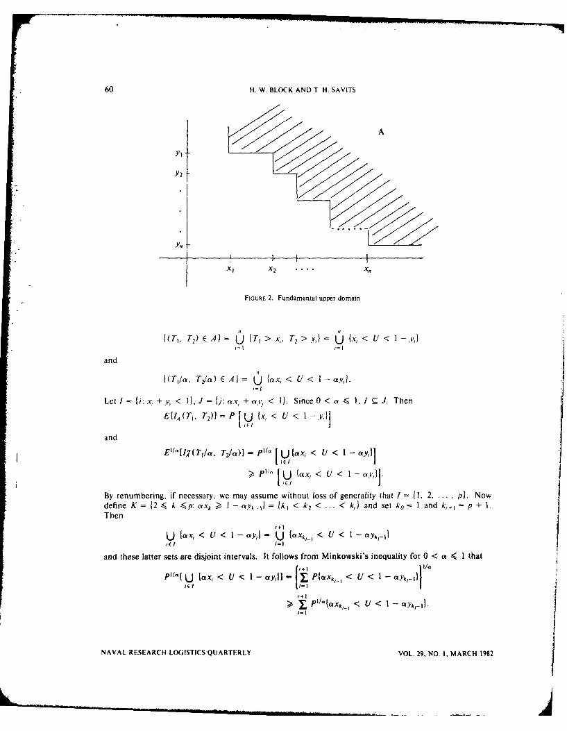
60 H. W. BLOCK AND T. H. SAVITS
A
Y2
yn
X1 X2 .... Xn
FIGURE 2. Fundamental upper domain
I(T1, T 2) E A = U 1T, > x,, T2 > VJ = U IX, < U < I -y,)
and
((T 1/a. T72 a) E A I U (ax, < U < I-a.v,.
Let I= i: x, + v, < ), J = {J':ax + aj, < I}. Since 0 < a < 1,/ 9 J. Then
E 1 , T1, T2)]= P U Ix, < U < I-.,]
and
EI/afI(T,/a, Ta)] = P"'[ U tax, < U < I- aYl]
> P1/" U (ax, < U < I - a,l.
By renumbering, if necessary, we may assume without loss of generality that I = {1, 2. p}. Nowdefine K= (2 (< k p:ax,. a I-.v, 1)= 1k, < k2 < ... < kJ and sel ko I and k,,i= p + 1.Then
r+1
U lax, < U < I - ayl - U {aXk, 1 < U < I - ayk,-1i( l 1- I
and these latter sets are disjoint intervals. It follows from Minkowski's inequality for 0 < a I 1 that
pl/,, U lax, < U < l-ay,i- P(axk, < U < I- yk,_l}El I aY-1)
r'+1
> ., PI/" l-l < < 1 Yk,- .
I-R
NAVAL RESEARCH LOGISTICS QUARTERLY VOL. 29, NO. 1, MARCH 1982
MIFRA LIFETIMES AND OTHER CLASSES 61
Since
U K < U < I -y ,= U U (X < U < I -y,,
it suffices to show that for / = I. r + I
P U (,, {.V-, < U < 1-,i < pil"lax,, I< U < I-ay,, 1).
But the union on the left hand side is contained in the interval {xk,_, < U < I -~lt and
Xk1_ + YA-- < I since for k1_ 1 < i < k, - 1, i E L And so we are done if we show that
- t < (I - a)I/ " for 0 < t K, !,0 < a - 1. This last inequality is, however, easily verified.
REFERENCES
[11 Barlow, R.E. and F. Proschan, Siatisuical Theory of Reliabiliy and L]iA' Testing: Probability .tlodel.(Holt, Rinehart and Winston, New York, 1975).
12] Block, H1W. and T.F. Savits, "The IFRA Closure Problem," Annals of Probability, 4, 1030-1032(1976).
[3] Block, H.W. and T.t. Savits, "Multivariate IFRA Distributions," Annals of Probability, 8, 793-801(1980).
[41 Block, [.W. and T.H Savits, "Systems with Exponential System Life and IFRA Component Lives,"Annals of Statistics, 7, 911-916 (1979).
[5] Esary, J.D. and A.W. Marshall, "Coherent Life Functions," SIAM Journal of Applied Mathematics,18, 810-814 (1970).
[61 Esary, J.D. and A.W. Marshall, "Multivariate Distributions with Increasing Hazard Rate Average,"Annals of Probability, 7, 359-370 (1979).
[7] Harris, R., "A Multivariate Definition for Increasing Hazard Rte Distribution Functions," Annals ofMathematical Statistics, 41, 713-717 (1970).
[8] Marshall, A.W. and M. Shaked, "A Class of Multivariate New Better than Used Distributions,"Annals of Probability, 10, 259-264 (1982).
VOL. 29, NO, I, MARCH 1982 NAVAL RESEARCH LOGISTICS QUARTERLY

REMARKS ON A UNIVARIATE SHOCK MODELWITH SOME BIVARIATE GENERALIZATIONS
William S. Griffith
University of KentuckyDepartment of Statistics
Lexington, Kentucky
ABSTRACT
In a 1973 paper J. D. Esary, A. W. Marshall, and F. Proschan [51 con-sidered a shock model giving rise to various nonparametric classes of life distri-butions of interest in reliability theory. A number of authors have extendedthese results in a variety of directions. In this paper, alternative proofs of theincreasing failure rate (IFR) and decreasing mean residual life (DMRL) resultsare given which do not make use of the theory of total positivity. Some bivari-ate extensions are then obtained using a shock model similar to that originallyused by H. W. Block, A. S. Paulson, and R. C. Kohberger [21 to unify variousbivariate exponential distributions.
INTRODUCTION
In a 1973 paper, Esary, Marshall, and Proschan [5] investigated a shock model which gives rise tovarious nonparametric classes of life distributions which are of interest in reliability theory, We willbegin this paper by reviewing these univariate life distribution classes and then stating the theorem dueto Esary, Marshall, and Proschan. We then provide new proofs to some parts of this theorem. Theproof uses elementary methods rather than results from the theory of total positivity. We will thendescribe a bivariate shock model which has been used by Block, Paulson, and Kohberger 12] to unifysome of the various bivariate exponential distributions which have appeared in the reliability literature.Finally, we will discuss a number of bivariate shock models yielding bivariate conditions that can beviewed as generalizations of the univariate new better than used (NBU) condition.
1. UNIVARIATE LIFE DISTRIBUTION CLASSES
In this section, we will consider various models of stochastic aging. For e'ery model of wearout(or adverse stochastic aging) there is an analogous model of improvement (or beneficial stochasticaging). Throughout, we will use the word "increasing" ("decreasing") to mean "nondecreasing" ("nonin-creasing" ).
Consider a single component or system with a random lifetime denoted by the random variable T.We will denote the distribution function of T by F. The survival function, denoted by F, isF(t) = P(T > 0 = 1 - F(t). We will assume throughout that ,F(--) = I (i.e., that Tis a nonnega-tive random variable). We now define the various nonparametric life distribution classes of interest.
If a life distribution F satisfies
(l.I F(t+x) is decreasing in-o < t < oo for fixedx > 0F(0)
then F is called an increasing failure rate (IFR) distribution.
VOL 29, NO I. MARCH 1982 63 NAVAL RESEARCH LOGISTICS QUARTERLY
pECED1NW PACIX BLANIL-LlOT FIJJED

64 W S. GRIFFITH
A distribution F is called an increasing failure rate average (IFRA) distribution if
(1.2) F(at) >, k'(t) for0 < a < 1, 1 > 0.
A distribution F is called a new better than used (NBU) distribution if
(1.3) F(x +y) < F (x)F(y) forx > 0, y >, 0.
A distribution F with a finite mean A is called a new better than used in expectation (NBUE) dis-tribution if
(1.4) F(x)dx < /F(t) for t > 0.
A distribution F with finite mean is called a decreasing mean residual life (DMRL) distribution if
(1.5) 1 f F(x)dx is decreasing in t.
For eaLai of the preceding classes of life distributions, there is a corresponding class which is amodel of beneficial stochastic aging. These are obtained from the preceding classes by replacingdecreasing with increasing, increasing with decreasing, and reversing inequalities. This results in classesknown as the decreasing failure rate (DFR) class, the decreasing failure rate average (DFRA) class, thenew worse than used (NWU) class, the new worse than used in expectation (NWUE) class, and theincreasing mean residual life (IMRL) class. We next discuss some alternate characterizations wh:chperhaps supply more intuition.
We begin by considering again a random variable T with distribution function F denoting the ran-dom lifelength of some device. For any x > 0, we will consider the survival function
(1.7) F(x + t)
Intuitively, F., represents the survival function of the residual life of the original device condi-tioned on the fact that it survived past time x. We next prove a lemma and a number of propositionswhich give alternate characterizations of most of these classes.
LEMMA i:
F, - (fOy-x fory > x > 0
PROOF: Omitted.
PROPOSITION 1: Let A, and / be the means of F and F, respectively.
(i) F has an IFR distribution if and only if <jz) < F,(z) for all zwhen x > v.
(ii) F has an NBU distribution if and only if F (:) < F(z) for all : when x > 0.
Let A be finite
(iii) Fis a DMRL distribution if and only if IA, g.t, for x > y > 0.
(iv) F is an NBUE distribution if and only if 1A A for x > 0.
NAVAL RESEARCH LOGISTICS QUARTERLY VOL. 29, NO. 1, MARCH 1982
UNIVARIATE SHOCK MODEL WITH BIVARIATE GENERALIZATIONS 65
PROOF: Omitted.
PROPOSITION 2:
(i) F is an IFR distribution if and only if F, is an NBU distribution for all y.
(ii) Let F have a finite mean. Then F has a DMRL distribution if and only if F, has anNBUE distribution for all y.
PROOF: The proof of (i) follows directly from Proposition 1 (i), Lemma 1, and Proposition 1(i).The proof of (ii) follows from Proposition I (iii), Lemma 1, and Proposition 1(iv).
2. THE EMP SHOCK MODEL AND THEOREM
In this section, we will discuss the Esary, Marshall, and Proschan (EMP) shock model andtheorem. We will provide alternate proofs to some of these results and indicate some generalizations.
We begin by defining various nonparametric classes of discrete distributions for positive integervalued random variables.
Let M be a positive integer valued random variable putting no mass at infinity. Then we shall say
that
(2.1) M is a discrete IFR random variable if (P(M > k)/P(M > k - 1) is decreasing in
k =1,2.(2.2) M is a discrete IFRA random variable if IP(M > k)}lk is decreasing in k = 1, 2.
(2.3) M is a discrete NBU random variable if P(M > k +j) ,< P(M > k)P(M > j) forj, k -0,1,2 ....
(2.4) M is a discrete NBUE random variable if P(M > k) i P(M > j) > P(M > j)j-O 0
for k = 0, 1, 2, ... and M has a finite mean.
(2.5) Mis a discrete DMRL random variable if IP(M > k)- P(M > j)} is decreasing
in k = 0, 1,2 ... and M has a finite mean.
Note that these classes of life distributions are simply discrete analogues of the classes that wehave previously defined in Section 1. If we reverse the inequalities and change decreasing to increasingwe can define analogous classes of discrete DFR, DFRA, NWU, NWUE, and IMRL distributions(except that we do not require M to have a finite mean in the NWUE and IMRL cases).
Next we describe the fundamental shock model discussed by Esary, Marshall, and Proschan.Consider a device subjected to shocks which occur in time as events of a Poisson process with intensityX. The device fails on the Mth shock where M is a positive integer valued random variable which is
Mindependent of the shock process. Letting T be the lifelength of the device, we see that T - X
where the X,'s are independent and identically distributed random variables having an exponentialdistribution with parameter X. The survival function is of the form
VOL. 29. NO. I. MARCH 1982 NAVAL RESEARCH LOGISTICS QUARTERLY
66 W. S. GRIFFITH
F(t)= P(T > t)= P(S(t) = k)P(M > k)k-0
where {S(t): t > 0) is a Poisson Process with intensity X.
We now state the main theorem.
THEOREM 1: (Esary, Marshall, and Proschan):
(i) If M is discrete IFR (DFR), then F is IFR (DFR)
(ii) If M is discrete IFRA (DFRA), then F is IFRA (DFRA)
(iii) If M is discrete NBU (NWU), then F is NBU (NWU)
(iv) If M is discrete NBUE (NWUE), then F is NBUE (NWUE)
(v) If M is discrete DMRL (IMRL), then F is DMRL (IMRL).
Elementary proofs of parts (iii) and (iv) were given in Esary, Marshall, and Proschan. The proofsof the remaining parts required results from the theory of total positivity. We now give proofs of (i)and (v) which involve elementary methods. We repeat the proof of (iii) to illustrate some techniqueswhich we will utilize. Furthermore, in the subsequent section, we use the techniques developed toestablish new bivariate results.
PROOF OF THEOREM I (iii): We note that
F0 + x)= P(S(t + x) = k)P(M > k).k-0
Since S): t > 0} is assumed to be a Poisson process, we have by the stationary independent incre-ments property that
00 k
F(t + x) I P(S(t) = A)P(S(x) = k - A)P(M > A + (k - A))k=O A=
= P(S(t) = A)P(S(x) = k -- A)P(M > . + (k - A))A-O k-A
= . (P(S(t) = A)P(S(x) = l)P(M > A + 1).A-0 1-0
Applying the discrete NBU condition on M we have that
F(f + x) i I P(S(t) = A)P(S(x)= I)P(M > A)P(M > I)A-0 1-0
= P (S (t) = A) P(M > A)) /0 P (S (x) = 1) P(M > l).
Consequently, T( + x) W F(t)F(x).
PROOF OF THEOREM I (i): Consider a random variable Twhose life distribution arises from a shockmodel in which M is discrete FR. In order to show that it is IFR It suffices from Proposition 2 that F,is NBU for all y. However, in light of the preceding proof, we need only show that F, arises from ashock model in which the random number of shocks survived has a discrete NBU distribution.
NAVAL RESEARCH LOGISTICS QUARTERLY VOL. 29, NO. I. MARCH 1982
UNIVARIATE SHOCK MODEL WITH BIVARIATE GENERALIZATIONS 67
Now
SP(S(y + U = A)P(M > A)-U F(y +u) .- 0
F(y) P(S(y) = j)P(M > j)1-0
X P(S(y) ~j, Sj(u) = A - j)P(M >1j + (A - j))a-0 j-0
iP(S(y) = j)P(M > j)j-0
where Sy (u) S S(y + u) - S (y)
j-0 A-j
SP(S(y) =j)P(M > j)j-0
S P(S(y) = j)P(S,(u) =k)P(M > j + k)j-0 k-0
SP(S(y) = j)P(M > j)j-o
SP(S(y) = j)P(M > j + k)
= P( 1 ,(u) =k) j0_k-0 I P(S(y) =j)P(Ml'> j)
j-0
Now the expression
SP(S(y) = j)P(M > j + k)
(2.6)SP(S(y) = j) (P(M > j)
j-0
is a function of k which has the value 1 when k =0 and is a decreasing function of k sinceP (M > j + k) decreases in k for fixed j. In addition, since M is discrete IFR, it is also discrete NBUand hence P(M > j + k) < P(M > j)P(M > k). Thus, the expression in equation 2.6 is boundedbetween 0 and P(M > k). However, as k - -c, P(M > k) - 0. Consequently, the expression inequation 2.6 is a survival function of a discrete random variable.
Next we let M* be a discrete random variable which is independent of the Poisson process(S,. t): t > 0) which has this survival function. Then , (u) is of the form
F, (u) P (S PS(u) = k) P(M* > k).k-0
To complete the proof we need only show that since M is discrete IFR, M* must be discrete NBU.
The condition that must be checked is
P(M* > k + 1) <- P(M> k)P(M* > 1).
VOL. 29, NO. 1, MARCH 1982 NAVAL RESEARCH LOGISTICS QUARTERLY

68 W. S. GRIFFITH
This is equivalent toP(S(y)=j)P(M>j+k+1) P(S(y)=j)P(M>j+k) P(S(Y)=j)P(M>j+
j~o <j=0 J-0, P(S (y) = j)P(M > j) P(S(y)=J)P(M >J) P(S(y) =J)P(M > j)
=0 _ =0 =__ 0
or after some algebra to
.(P(M > j + k + I)P(M >A) )- P(M > j + k )P(M > .1 + M)P(St(y) = A)P(S(J,)=.j) < 0.
Since for A < 0 or j < 0, P(S(y) = A)P(S(y) = J) 0 0, we may rewrite the above condition as
. (P(M>j+k+I)P(M>A)-P(M>j+k)P(M>A+I))P(S(y)=A)P(S(y)=j) <0.A=-oo J=- o
By breaking up this double summation into three parts: over A < j + k, I = j + k, andA > j + k, realizing tht the middle term of the preceding sum is zero; letting A'= j + k andj'= A - k so that j = A'- k and A = j' + k (with the consequence that the condition A > j + k isequivalent with j' + k > A') and rearranging, we then find that the condition we are checking can berewritten as
. ,(P(M > j + k + I)P(M > A)- P(M >j + k)P(M > A + I))P(S(y) =A)P(S(y) =j).I<J+k
((P- (M >(P + j + I)P(M >A) -P(M>ji+k)P (M > A + MI<j+k
P(S(y) = .j + k)P(S(y) = A - k)} 0,
or
( {(P(M > j + k + I)P(M> A)- P(M > j +k)P(Af > A + )).A< +k
(P(S(y) = A)P(S(y) = j) - P(S(y)=j + k)P(S(v)=A - k))) < 0.Noticing that
P(M > j + k + 1)P(M > A) - P(M > j + k)P(M > A + 1)
S(M > j+ k+ 1 P(M> A +I) P (AM>]+ P I A= (P(M >j + k) - P (M >A) j + k)P(M > A) 0
since M is discrete IFR and A < j + k, we see that it now suffices to show only that
(2.7) P(S(y) = A)P(S(y) = j) - P(S(y) = i + k)P(S(y) = A - k) > 0.
We may take care of a number of cases rather easily. If A < 0, then A - k < 0 and the left hand sideof (2.7) is0- 0= 0. If A > 0 andj < 0, thenA - k < 0sinceA <j + k. Thus, the left hand sideof (2.7) is 0 - 0 = 0. If 0 < A < k andj > 0, then the expression on the left hand side of (2.7)reduces to the nonegative quantity P(S(y) = A)P(Sv) = j). Finally, we consider the case whereA> k and j > 0. First, note that if A > k and A < j + k, then j ;4 0. If k = 0 then (2.7) isimmediate, thus we consider k > 0. The left hand side of (2.7) is
e-A.V(Xy)a e-.(hy)J e-Y(Ay)j+l e-)A (Xy)-1-k v
A! j! (J+k )! (.-k)!- e- 2A-(Ay ) +e A ('\y + , I) {(j + k) (J+ k- 1) ... (j + 1) -. (, -1 ..(A. - k, + I)
which is clearly nonnegative if A < j + k. This completes the proof.
NAVAL RESEARCH LOGISTICS QUARTERLY VOL. 29, NO. 1, MARCH 1982

UNIVARIATE SHOCK MODEL WITH BIVARIATE GENERALIZATIONS 69
Next, for the proof of Theorem I (iv), we refer the reader to the paper of Esary, Marshall, andProschan. We now show that (v) of Theorem I follows from (iv) in much the same fashion that (i)followed from (iii).
PROOF OF THEOREM I (v): Consider a random variable Twhose life distribution arises from ashock model where M is discrete DMRL. In order to show that it is DMRL, it suffices from Proposi-tion 2 to show that F is an NBUE distribution for all y. However, in light of (iv), we need only showthat F arises from a shock model in which the number of shocks survived has a discrete NBUE distri-bution. Now as before it can be shown that
SP(S(y) = j)P(Mf>j + k)FY(u) - P(Sy(u) = k) J-0
k-o P(S(y) j)P(M > j)
j-0
Again, we can show that the expression
P(Sv(y) = j)P(M > j + k)j-0
, P(S(y) = j)P(M > j)j-0
is the survival function for some discrete distribution.
Now if, as before, we let M* be a discrete random variable which is independent of the Poissonprocess (S,(t): t > 0) and has this survival function, then F,. (u) is of the form
F, (u) =, P(S (u) = k)P(M* > k).k-0
To complete the proof it will suffice to show that M* is discrete NBUE since M is discrete DMRL.That is, it will suffice to show that
(2.8) (P(M* > W)-1 P(M* > k) < . P(M* > k).
k-1 k-O
This can be simplified to
P P(S (y) -j) P(M > j + k) P P(S (0) j) P(M > j + k)(2.9)j-0 k-I < j-o k-0
P(S(y) = j)P(M > j + I) I P(S(y) = j)P(M > j)j-0 '1-0
Now after some algebra we may rewrite the condition from (2.9) as
j7 j (iP(S(y)-- j)P(S(y) = A)P(M > j + l)P(M > A)j-O A-O
IP(M > k) - .P(M > j + ) + P(M > A) k- P(M> k)
VOL. 29, NO. I, MARCH 1982 NAVAL RESEAR( 14 LOGISTICS QUARTERLY
70 W. S. GRIFFITH
Since for j > 0 or A < 0, P(S(y) j)P(S(y) A) = 0, we may rewrite the preceding as
P > (Sy) j)P(S(y) I)P(M >1+ flP(M> A)
1 P(M>J +I ~ ( ~ P(M >A) i P(M > k)Jj(> Tk-kA
By breaking the summation into three parts and using methods analogous to the IFR case we canjustify this inequality and thus complete the proof.
3. A BIVARIATE SHOCK MODEL
Now consider two devices which are subject to shocks. We will denote the number of shocks todevices 1 and 2 in [0, d by S 1(t) and S 2(t), respectively. Further, we let (MI, M 2) denote the randomnumber of shocks until failure of devices I and 2, respectively. Block, Paulson, and Kohberger [2]have unified some of the various bivariate exponential distributions in the reliability literature by taking(M], M 2) to be a bivariate geometric distribution with joint survival function given by
PlI' (P01 + P1) m 2 m if m1 I< M2P(Ml > M, M2 > M2) = MpP 2 (plo + pil) 'n -
2 if n 2 < M 1
where Poo + P + [ 10 +pu= l, Pl0 + p l < 1, and po + pl < 1. If we take SI() =S 2 (t) to be thesame Poisson process, then (TI, T2) will have a Marshall and Olkin bivariate exponential distribution.If SI(t) and S2(t) are taken to be independent Poisson processes the resulting joint distribution of(TI, T 2) turns out to be of the type which has been discussed by Downton [41, Hawkes [61, and Paul-son [81 depending on the choices of the various parameters. Consequently, in this section, the modelin which the shocks occur simultaneously to the two devices, i.e., S1 (1) S2(t), will be called theMarshall-Olkin type of shock model, while the model in which the shocks occur according to indepen-dent Poisson processes will be called the Downton-Hawkes-Paulson type of shock model. We will nowconsider various bivariate discrete NBU conditions on (Mi, M2) which yield bivariate NBU conditionsof the type considered by Buchanan and Singpurwalla [3].
Marshall-Olkin Shock Models
Consider two devices subject to simultaneous shocks occurring according to a Poisson process.Letting M, and M 2 represent the number of shocks until failure of devices I and 2, respectively, wewill prove some results about H(, t2) = P(TI > tt, T2 > t2) where T, and T 2 are the respective life-times of the devices.
PROPOSITION 3: If P(MI > m1 + j, M 2 > T 2 + A)< P(MI > T 1 , M 2 > rn2)P(MI >j,M 2 > i) for all nonnegative integers ml, M 2, j, then H(t, + x, t2 + x) < H(r, t2)H(x, x) for all t,t2, x > 0.
PROOF: We will prove this for t, < t2. The proof for the case where t, > t2 is analogous.Throughout the proof we will make crucial use of the stationary independent increments of the Poissonprocess. We begin by writing for ti < t2
F(It, t2) - i y P(S(t 1 ) = ki, S(12) = k2)P(M 1 > k1 , A12 > k2).k,-0 k2-k1
NAVAL RESEARCH LOGISTICS QUARTERLY VOL. 29, NO. 1, MARCH 1982
UNIVARIATE SHOCK MODEL WITH BIVARIATE GENERALIZATIONS 71
By using the stationary independent increments property, we may rewrite this as
(3.1) H(t1, t2)= . P(S(t) = k) , P(S(t 2 - ti) = i)P(M > k, M2 > k + i).k=0 i1O
In an analogous fashion we may then also write for fixed, but arbitrary x >, 0,
H(t + x, t2 + x) = , (P(S(t1 ) = A)P(S(x) = k - A)P(S(t 2 - td = i)k-0 A-0 -- O
P(M1 > kM 2 > k + i))
by using the stationary independent increments property. Next by interchanging the orders of summa-
tion and performing some algebra it can be shown that
H (t I + X, t2 + X)= f(S(th) A 40 P(S(t 2 - td = i)P(MI > A, M2 > A + i)i-o
P(M] > A + M 2 > A + i + i))1 (o P(M] > A, M 2 > A + i)
By using the NBU assumption on (MI, M2), we have
H(t I + x, t2 + x) < P(S(t) A) P(S(t 2 - t) -)P(M > A, M 2 > A + i)
P(S(x) j)P(MI > J, M 2 > J)
Rewriting the right-hand side of the above inequality we have
(3.2) H(tt + x, 12 + x) < H(tl, t 2)H(x, x).
We remark in passing that if the direction of the inequality in the hypothesis of the preceding proposi-
tion is reversed, then the inequality in the conclusion is reversed. This would be a model of stochastic
improvement with age. We also note that the boundary distributions (ones in which equality holds in
equation (3.1)) in this case are the distributions with the bivariate loss of memory property. If
exponential marginals were required, the boundary would be the Marshall-Olkin bivariate exponential
distribution.
PROPOSITION 4: If P(MI > m1 + Jt, M2 > m2 + J2) < P(M] > m1, M2 > m 2)P(Mt > it,l 2 > J2) for all nonnegative integers M1 , M 2 , J., i2 with (M - M2 ) (J1 - J2) >1 0, then
H(t1 + x1, t2 + x 2) < H(t1 ,t2)If(x, x 2) for all tl, t2, X1, x 2 >1 0 with (1 - t2) (xI - x 2) > 0.
PROOF: We first assume that it < t2 and x, < x 2. As we have seen in equation (3.1) of theproof of Proposition 3
H(ti, t2) = P(S(t 1 ) = k) , P(S(t 2 - t1) = i)P(MI > k, M 2 > k + ).k-0 i-O
Now we may write H( 1 + Xt, t2 + x 2) as
H(01 + x1. t2 + x 2) = (P(S(t, + xt) = k)P(S(12 - t1 + x 2 - x) =
k=0 i-O
P(MI > k, M2 > k + i)).
Now by using the stationary independent increments property, interchanging the order of summation,
and performing some algebra, we can show that
VOL. 29, NO. I, MARCH 1982 NAVAL RESEARCH LOGISTICS QUARTERLY
72 W. S. GRIFFITH
H(1 + xi, t2 +x= X2 P(S(t1 ) = A) P P(S(t 2 - t1) = n)P(Ml > A, M2 > A + n).1-0
P(MI > A + j, M 2 > A + i + n +m)
P(M] > A, M 2 > A + n)
Using the condition on (MI, M 2) given in the hypothesis of this proposition we then have that
H(01 + x 1, t2 + x 2) P(S( 1) = A) P(S(t 2 - )= n)P(MI > A, M2 > A + n)
P P(S (xJ) j) P(S(X2 - X1) -m)P(M 1 > j, M2 > i + M11=0 n=0
But the right-hand side of the preceding inequality is just 1(t 1 , t2)H(x, x 2). Thus, we have for
0 < 1< t2 and 0 < x, < x2 that
(3.3) R0(, + x1, t2 + x2) < H(t, t2) H(x,, x2).
For , > t2 > 0 and x, 1 X2 > 0, an analogous argument will lead to equation (3.3). The boundarydistribution (in which equality holds in equation (3.3)) turns out to be the Marshall-Olkin bivariateexponential distribution. Also a reversal of the inequality in the hypothesis of this proposition leads toa reversal of the inequality in the conclusion. This is a model of stochastic improvement with age.
Marshall and Shaked [71 have considered a cumulative damage model in which the damages(Dl,. D 2 ) are independent and identically distributed random vectors with a joint distribution functionG. Then if d, and d 2 are the fixed failure thresholds of the devices, then the survival function of(M, M 2) has the form
P(MI > MI, M2 > M2 = P D1, dl, D 2i < d2j.
Marshall and Shaked prove that when the survival function of (MI, M 2) is of this form that thehypothesis of the preceding proposition is satisfied. Consequently, the joint survival function of thedevices satisfies equation (3.3) for (tj - t2) (xI - x 2) 1> 0.
PROPOSITION 5: If P(MI > m + j, ML> m + j) < P(M, > m, M 2 > m) P(MI >,M 2 > j) for all nonnegative integers m and j, then H(t + x t + x) < H(0, t)H(x, x) for all t, x > 0.
PROOF: By the stationary independent increments property we can write
(+x, t + x) = i i P(S W = k)P(S(x) = j)P(M I > k + j, M 2 > k + j).k-0 j-0
Using the hypothesis of the proposition, we have
F1 + x, I + x) < P(St) = k)P(S(x) = j)P(M, > k, M 2 > k)P(MI > j, M 2 > J).k-0 j-0
The right-hand side of the preceding inequality can be rewritten to yield
F(1 + x, t + x) y (t, t)F(x, x).
NAVAL RESEARCH LOGISTICS QUARTERLY VOL, 29, NO. I, MARCH 1982
UNIVARIATE SHOCK MODEL WITH HIVARIATE GENERALIZATIONS 73
Finally, we will conclude this section with a counterexample. The question is whether a discreteNBU condition
P(M > Mt + Jl, M2 > M2 + J2) < P(Ml1 > M, M2 > m2)P(Ml > Jl, M 2 > J2)
for all nonnegative integers ml, M2 , Jl, j2 would imply the continuous analog
H(01 + xl, t2 + x 2) < H(t1 , t2)H(xl, x 2) for all ti, t2, x 1 , x 2 > 0.
The following counterexample answers this question in the negative. Suppose that M, and M 2 aredegenerate random variables with M, = 1 with probability I and M2 = 2 with probability 1. It can be
shown that P(MI > ml + jl, M 2 > m 2 + j2) < P(M > Ml, M 2 > m2)P(l > Ji, M 2 > 12) and
that if t, < t2 , xI > x2 and tl + x, > t2 + x 2,
H(1 + xl, t2 + x 2) - H(1, t2)H(xi, x 2) = e- ' ' (x tk))
> 0.
However, an NBU result along these lines does hold in the case of the Downton-Hawkes-PaulsonShock Model.
A Downton-Hawkes-Paulson Shock Model
In this model we consider two devices subject to shocks occurring according to independent Pois-
son processes. Let I(Sl(t): t > 01 and {S2(t): t > 0) be these processes and (M, M 2) be the random
number of shocks until failure of the respective devices.
PROPOSITION 6: If P(M > ml + jl, M2 > M2 + J2) < P(Ml > j_ M2 > m 2)P(Ml >
JL, M 2 > J2) for all nonnegative integers in, m2 , Jl, J2, then H( + xl, 12 + x 2) <H(01 , t2)H(xl, x 2) for all tl, t2, x 1, x 2 > 0.
PROOF: By the stationary independent increments property P- I an interchange of the order of
summation we have
HG( + x 1 , t2 + x 2) = 0 P(SI(x1 ) = M, S2(x 2) = n)P(AM, > Me, M2 > n)m-0 n-0
k-m j-n
P(M > k, M 2 > J)
( )= k- , S2 (t2)=j-n) P(M > m, M2 > n)
Using the hypothesis of the proposition, we can write
HG 1 + x1, t2+x 2) (P(Sl(xl) = m, S 2(x 2) = n)P(MI > Mn, A 2 > M)1-
0 n-0
P(Sl(tl) = k - m, S2(02) = / - n)k-m j-n
P(M > k- M, M2 > J- n)).
By a change of variables
H0'1 + x 1, 12 + x 2) < l P(SI(x1 ) M, S 2(x 2) = n)P(MI > m. M2 > n).
SP(S 1 01 ) = k, S 2(t2) 00 )P(M 1 > k, Al2 > i)j.
k-0 j-0
But the right-hand side of the preceding inequality may be rewritten as H(¢,. 12)H(x 1 , x 2), thus com-
pleting the proof.
VOL. 29, NO. I. MARCH 1982 NAVAL RESEARCH LOGISTICS QUARTERLY
74 W. S. GRIFFITH
REFERENCES
[11 Barlow, R.E. and F. Proschan, Statistical Theory of Reliability and Life Testing (Holt, Rinehart andWinston, New York, 1975).
[21 Block, H.W., A.S. Paulson and R.C. Kohberger, "A Class of Bivariate Distributions" (submitted forpublication).
[31 Buchanan, W.B. and N.D. Singpurwalla, "Some Stochastic Characterizations of Multivariate Sur-vival," The Theory and Applications of Reliability with Emphasis on Bayesian and NonparametricMethods," Vol. 1, C. P. Tsokos and I.N. Shimi, Editors (Academic Press, New York, 1977).
[41 Downton, F., "Bivariate Exponential Distributions in Reliability Theory," Journal of the Royal Sta-tistical Society, Series B, 32, 822-830 (1970).
[51 Esary, J.D., A.W. Marshall and F. Proschan, "Shock Models and Wear Processes," The Annals ofProbability, 1, 627-649 (1973).
[61 Hawkes, A.G., "A Bivariate Exponential Distribution with Applications to Reliability," Journal ofthe Royal Statistical Society, Series B, 34, 129-131 (1972).
[7] Marshall, A.W. and M. Shaked, "Multivariate Shock Models for Distributions with IncreasingHazard Rate," The Annals of Probability, 7, 343-358 (1979).
[8] Paulson, A.S., "A Characterization of the Exponential Distribution and a Bivariate ExponentialDistribution," Sankhyi, Series A, 35, 69-78 (1973).
NAVAL RESEARCH LOGISTICS QUARTERLY VOL. 29, NO. I, MARCH 1982
ASYMPTOTIC JOINT NORMALITY OF ANINCREASING NUMBER OF MULTIVARIATE ORDER
STATISTICS AND ASSOCIATED CELL FREQUENCIES
Lionel WeissCornell UniversityIthaca, New York
ABSTRACT
Take n independent identically distributed (liD) observations from a con-tinuous r-variate population, and choose some order statistics from each of ther variates. These order statistics are used to construct a grid in r-dimensionalspace. Under certain conditions, it is shown that as n increases we can choosean increasing number of order statistics in such a way that the asymptotic jointdistribution of the chosen order statistics and of the frequencies of samplepoints falling in the cells of the grid can be assumed to be a normal distribu-tion An application to testing independence of random variables is given.
1. NOTATION, ASSUMPTIONS, AND STATEMENT OF THEOREM
We observe n lID r-tuplets (X1 (i). X,(i)), i = I. n, each with joint cumulative distri-bution function (cdf) F,(xi .... Xr), joint probability density function (pdf) fn(xt .1 x,). Wechoose a set of order statistics from (XI(), ... , X,(n)), a set of order statistics from(X2(). X2(n)),.. and a set of order statistics from (Xr(I)- Xr(n)). These chosen orderstatistics are used to construct a grid in r-dimensional space. This grid defines a system of r-dimensional cells, each cell having a frequency of sample points falling in its interior. It is clear fromthe argument of [I] that if the number of chosen order statistics for each variate is fixed, then undermild conditions the joint asymptotic distribution of the chosen order statistics and the cell frequencies(all properly standardized) is normal. But for certain purposes, it is necessary to let the number oforder statistics chosen increase as n increases. In this paper we show that under certain conditions westill get a joint asymptotic normal distribution.
For typographical simplicity, until Section 3, we discuss only the case r = 2, and we write the nlID pairs observed as (X ), Y) (X2. .... (X,, Y,). The joint cdf and pdf for (XI, Y1) will bewritten as F,,(x, y), f,(x y), respectively, and so are allowed to depend on n. G,(x), g,(x) denote,respectively, the marginal cdf and pdf for X1. H,(x), h,(x) denote, respectively, the marginal cdf and
pdf for Yl. Define F,,'1 (x * y) as -L F.(x, Y)]x-v, and F, 2) (X, yi asLax ay
For each n, choose p,,, q,, and L, so that 0 < p, < q, < 1, and np., nq., L,, and
K- =- are all positive integers. These quantities also are to satisfy other conditions to be
specified below.
Xl' I < ... < X,, denote the ordered values of (X1. X'), and Y'l < ... < Y/, denote theordered values of ( Y..... Y,). X*, denotes X(,,,. + 0, - t l and Y; denotes Y + ,-)L.l for
VOL. 29, NO. I, MARCH 1982 75 NAVAL RESEARCH LOGISTICS QUARTERLY
76 L. WEISS
i 1-. K, + 1. Let ND(n) (for "No duplication in n observations") denote the following event:there is no pair (X;, Y') with X among (X.. X.+,) and Y' among ( Y.. Y.+l). We assumethat (f,,, p, q., L,,} are such that lim P[ND(n)] = 1. This assumption will be discussed in Section 3:
n- ounder it, for all asymptotic probability calculations, we can (and will) assume that ND(n) occurs for alln.
Define X* as supix: G.(x) - 0), X .+2 as infix: G,(x) = 1), Y* as suply: H,(y) = 0), and Y*.+2as inf(y: Hn (y) = 1. Thus, these values may depend on n, and may be -- or oc.
Define N,, as the number of pairs (X,, Y,') in the open rectangle in (x. y)-space defined by(X,*_ < x < X,'. Y*-I < y < Y7), for i, jranging between I and K,, + 2, inclusive. Define Sj] as 1 ifthe Y' originally associated with X* falls in the open interval (Y*_1. Y1) and as zero otherwise, fori = 1 .... K,, + 1 and j = 1 .... K,, + 2. Define TJ, as 1 if the X' originally associated with Y)' fallsin the open interval (X,*1 , X,) and as zero otherwise, for j = 1. K + I and i = 1. K,, + 2.The occurrence of ND(n) then implies all the following equalities:
A,+2
S,,= 1 for = i.. K, + 1,'-I
A,,+2T, =,= for j=1. K + ,
Kn+2 K.+1Nj N~+ Tjl riP.- 1,
i-I i-I
K,+2 K.+I
(1.1) 7 Ni+ I T,= Ln - I fori=2. Kn+ 1,1j-1 j-I
K,+2 Kn+I
E NK,,+ 2.i + I T.K,,+2 = n - nq,i-I j-1
Ka+2 K,+lN, 'I+ 1: SI riP,- 1,
i-I i-I
A,+2 k.+
I N,, + I S, =L, - Iforj=2 . K.+I,t I i-I
An+2 K.+1
5 N,.,,+ 2 + 5,.K,+2 - n - nq,.
i-I i-I
Let G( - I, n) denote G,- 1n'P + (0 L for i = 1. K, + 1, define G(-I, n) as Xa,
and G(K .In) as +'1 4+2. Let H(j -1, n) denote H."- + n I)L,, for j-1 ... K
and define H(-1, n) as Yo*, H(K + 1. n) as Y,.+ 2. Let k(i - 1. n) denote g(G(i - 1, n)) fori- 1. K,, + 1, and h(j - 1, n) denote hn(H(j - I. n)) forj - I. K. + I. Note that thesedefinitions imply that F,,(G(i - 1. n), H(K, + 1, n)) - ,(i- 1, n), andF,,21(G(K, + I. n). H(j - 1. n)) - h(j - 1. n).
NAVAL RESEARCH LOGISTICS QUARTERLY VOL. 29, NO. I, MARCH 1982

ASYMPTOTIC JOINT NORMALITY OF MULTIVARIATE ORDER STATISTICS 77
Next, define X, as .vn (i - 1, n) (X-- G(i - 1. n)) for i = 1. K" + i, and define X0 as 0
and Xh,+2 as 0. Define Y, as v h (j - 1, n)(Y - l(j- l. n)) for j= . K, + 1, and define
Yo as 0 and Yt +2 as 0.
For i= 1. K, + 2and j= . K, +2, define Q, as
+ F 2' (G(i - 1, n), H(j - 1. n)) Y,/h(j - I. n)
- F,"'(e; 0 - 2. n), F Q - 1, 0)) X,- Ilk,( - 2. n)
- Fn2 ' (G(i - 2, n), H(j - 1, n)) YIh(j - 1, n)- F,.,(G - . n), TIl(i - 2, 0)) X,/1(i - 1, n)
- F(21(G(i - 1. n). H(j - 2. n)) Y,/-h(j - 2. n)+ F,"(G(i - 2. n). Hf(j - 2, n))X.I/(i - 2. n)
+ F"(21(G(i - 2, n), H(j - 2. n)) Y, 1/h(j - 2. n)
where any term containing X0, X "+2. Y0, or YA,,+2 is defined to be zero. It follows from the definitionsA.+2 A,+2 Kn+2that 7 _~ xj = xYa foorAv
Q, = X,- X,-so Q, = X,.fora= 1. K,,+2. Similarly, ' Q,= Y,3 for/-I -1 j-1 j-l i=1
.. K,,+2.
Define p,,(i, j) as the probability assigned by F,(x, y) to the rectangle (G(i - 2, n) <
x < G(i - 1. n), H(j - 2, n) < y < Ff(j- 1,n)) for i= I. K,+2, j= K,.... K +2.
Define W, as Ni - npi.( j) and Z, as W -, for i=l. K,,+2 and
j= . K,,+2. Then we have
A,+2 A,+2 -2(K, + 1)I I -\p .j)z, 4= r1-1 i-I
a A'+Ii-I i-I
a& +2 1: X '
(1.2) 1 ' z,,= i - KX,
fora = 1. K, + 1.
A +2 -Z , s,-3-I i I- y
i-I i-I
for/3= 1. K, + 1.
Let g; denote min (g(x): G,-'(p,) < x < G,-7(q )}, h. denote minh,(y): H,-I(p,) <
y < H j(q,,)I, b, denote minfg*, h.*} and c,, denote minlf,,(x,y): G-I(p,) < x < G-(q,),
H-(p.,) < y 1< HNE-L(qI)A.
VOL. 29, NO. 1, MARCH 1982 NAVAL RESEARCH LOGISTICS QUARTERLY

78 L. WEISS
We assume the following:
(1.3) f(x, y), F,,' (x, y), F,,(11(x,y),
-A- g, (x)l -y h.,(y)' --t 4f (x,Y) ,
and - f. (x.y) are all bounded, for all values of x,y, and n.lay I4)min17 Q = 0m = 0 (j(14)mm0ij) K K 2 ' (ij) K
(1.5) There exists a finite value b so that b. < b for all sufficiently large n.
K 15
(1.6) n approaches zero as n increases.
(1.7) , approaches zero as n increases.
Denote by f[ the joint pdf for the random variables (Se, Ti, X, Y', Wi,}.
Now we construct an "artificial" joint pdf for the random variables TSij, f. A', Y, Wj}, as fol-
lows. The 2(K, + 1) + 1 sets of random variables (S,- ,A±.K.+21 for i = 1. K, + 1,
T l. Tj.K+2) for j- 1 ... , K. +1; and (Zi: -1 ... , K,+2; j= 1. K.+2;
(iJ) (K. + 2, K. + 2)) are independent of each other. The joint distribution of {Sl. Si.&+2}K.+2
is given as follows: each Sq is0 or 1, 7, So = 1, andi-i
[F,(") (G(i-l,n),H(j-l,n)) - F(l)(G(i-l,n),H(j-2,n))JP (S , = 01)= n(- I. n)
AK+2
The joint distribution of .Tjl Tj. A-+2) is given as follows: each T,, is 0 or 1, Ti, = 1, andI-I
P(Tji= ) = [F 2 1((i-l.n),H(j-1l,n)) - F(2)((i-2,n),T(j-l,n))]
h(j-l, n)The (K. + 2)2 - I random variables IZj: i - 1. K. + 2; j - 1,. K. + 2;
(iJ) * (Kn + 2, K. + 2)) have the following joint normal pdf:
I-lA,., )2 - IIA, +2 A. ±2(2-'2f t-( '+ )2 (p, (K, + 2, K" 2)) exp- . zi
K.+2 K,+2where ZA.+2.A,+2 is given by the identity I I z,, - 0. For future use, we note that in this
j-I i-Idistribution, the variance of Z is 1 - p,(i,j), and the covariance between Z,, and Z,,, (where(i.j) d (i'.j')) is -. p,(iij)p1 ,(i',j'). Now define (X, A. ,X+,, Y1 ... )'A,+,) in terms of
IS,,. T,,. ZJ by means of equations (1.2). Defining Q,, as above, define W,, as Z,, + for
NAVAL RESEARCH LOGISTICS QUARTERLY VOL. 29, NO. I, MARCH 1982
ASYMPTOTIC JOINT NORMALITY OF MULTIVARIATE ORDER STATISTICS 79
i < K, + I and j < K, + 1. Then define W, as the closest value to Wj that makes np,,(ij) +KA+2
)W,/ an integer (positive, negative, or zero). Finally, define W,,K+ 2 by the equation
K.+2 Kn+2 K,+2 K,+2W. N,, - n p,(i,j), WA+2, by the equation np Q W, = , N,,-n
,-I i-I i-I i-IA,+2 &,+2 A,+2 K +2
E Pj(iJ), and WA +2.k +2 by the equation V p 0 JW, = -2(K, + 1), where : N,, and
K,+2
N, are defined by the equations (1.1).t-1I
Denote by f, the joint pdf for the random variables (9,. Ti, Ti , Y', W,} induced by the processjust described.
For any measurable set C, in the space of (Sj. Ti, ki,. Y, W,1 }, let Pf(C,), Pf.(C) denote the
probabilities assigned to C, by ., and fin, respectively. In the next section, we prove the following:
THEOREM: lim sup IP- (C,) - P. (C,) = 0.C A
2. PROOF OF THE THEOREM.
The theorem combines the results of [1], 121, and [31, and the proof is a combination of theproofs in those papers. First we list some notation and elementary results that will be used in theproof.
The symbol "log' always means the natural logarithm. For any event E, E denotes its negation.4(x) denotes the standard normal cdf. If we state that a sequence of random variables { V, is
00(r0(n), it means that l converges stochastically to zero as n increases, for an arbitraryrn) ( (n)
sequence p3(n) with /3(n) approaching oo as n increases. Thus, if (VJ is 0p(r(n)) and r(n) approacheszero as n increases, then V, converges stochastically to zero as n increases.
The following equalities and inequalities are well-known:
m(2.1) For any events El . E, P(E, nl ... n Em) > I - £ P(E,) (Bonferroni' s ine-
quality).
1 -' 2(2.2) For any x > 0, 1 - (Dx) < , e
(2.3) For any positive integer m, log m! Iog2r + m + I-logm- m + W W
where 6w(m)I < I. (Stirling's formula).
(2.4) If V is any random variable with P(V < 0) - 0, and if b is any nonrandom positivevalue, P(V < b) > I - E(V) (Chebyshev's inequality).
- - b
X2 X3
(2.5) If IxI < l, log(l+x)=x--:- + x) where 11 < 1.2 3 (1 + 9x)3
VOL. 29, NO. 1, MARCH 1982 NAVAL RESEARCH LOGISTICS QUARTERLY
80 L. WEISS
LEMMA 2.1: If V1. V, are jointly normally distributed, with zero means, variances.2 .... , . respectively, and any covariances, and if ( denotes max (a .. o',), then for any
c > 0, P [max Xj < cI > 1 l - ex 2mc '*
PROOF: A combination of (2.1) and (2.2).
LEMMA 2.2: Under both f,, and f ,
(max IX, //-nVk(i - 1, n)} = 0 Kn 1, and (max iY 11,1n- (j - 1, n 0,p1 1i-I. Kn+l rnb,j j= 1...., K.+I I J
PROOF: We only have to give the proof for X,, since the proof for Y is the same. Under f., wecan assume the joint distribution of {X,.} is the normal distribution described in [2], and then set
K.c in Lemma 2.1, completing the proof. Under f*,, using equations (1.2) we note that
In, b,,+2&+(-1K, + 2 , and that the variance of N 0J 7( Zij is less than
one. The result then follows directly from Lemma 2.1.
LEMMA 2.3: Under f4, {max I W0 1/,J}p =Qj 0,
PROOF: Let (3,} denote a sequence of nonrandom positive quantities such that lim /3, =.. , nK)n
and lim 8 = 0. Let Nj denote the number of (X. Y;) falling in the open rectangle,,-- b,,n
(G(i - 2, n) < x < G(i - 1, n), H(j - 2, n) < y < H(j - 1, n)); let NJ°1 denote the number of(Xi, Y') falling in the open rectangle
G( 1 np, + (i- 2)L, /3 K, 1 np + (i- 1)L, /3,K,,
,, (np,, + (-2)L, + n < y < H1( ~)n n& + (j
and let NJ2) denote the number of (Xi', Y) falling in the open rectangle
G,- nG + (i- 2)L, < x < ,K np,+ G , + i , 1)LK
it np.,+ (j -2) L,, 8,,K, < ip, + (i -1) Ln ,K
n rn/-n~ b < H n -vn b,
(G,-'(a) is defined as X if a < 0, and as XK*+2 if a > 1; Hn'(a) is defined as YJ if a < 0, and asYK%+2 ifa > 1).
Clearly, N 0 ) < N 9 ) < N 121, and by Lemma 2.2 with probability approaching one as n increases,we have NJ) <y N < N 2 . Now NJ21
- N,0 is the number of pairs (X,', Y') which fall in a region2/3,,K,,
consisting of pieces of four strips, each strip having probability (under *f) no greater than 2/8,----8n/3,K.,
Therefore, E(Nj2) - NJ°0)} < .n-, and using (2.1) and (2.4), if t3 is any positive value,
NAVAL RESEARCH LOGISTICS QUARTERLY VOL. 29, NO. I, MARCH 1982
ASYMPTOTIC JOINT NORMALITY OF MULTIVARIATE ORDER STATISTICS 81
p IN 2 ,. (0)8n (K. +2) 2 K[/3
PIN"' - Njol < 3,, for all ij] >1- . Below we will choose 3,, and 6, so that
approaches zero as n increases; then we can say that with probability (under f,) approaching
one as n increases, we have INij - NJi" -<, for all i j.
/V()- tip,, 0, j)Ni] -np(i, j) -Now define W,(" ) as Then with probability (under .f) approaching one as n
increases, W _ '1j < 9_1 for all i, j. But by [3] and Lemma 2.1,inrass / n ) 0 np-0 nPn G, j)
m WP I 0p Since On can increase arbitrarily slowly, we can let An increase at1max npi )1 0 fK " .Snef, a rirrl e ,~,a
any rate that makes - approach zero as n increases. This completes the proof./3.b,
LEMMA 2.4: Under fl, ({max IWij 1/} (ij)I = op b n/-.
PROOF: For i and j both less than or equal to K, + 1, W. is within I of W11 and
V 2,' p, 0, j)
W', - Z' + Ij. Applying Lemma 2.1 to {Zj} and (Q1V, we immediately find that under f .Ii: K" 'm a W I VK 2 ',/
-ff - "b K +2
) I = N+2a= . Since , Q j) Wj is 0,(K,), we see that.K,' np,=Q j ) J ,-
I ,+ 2I ' K(',oK , an IWK +21 L..O $.JikFrm max " 1 " and max np=KO+p)~1<=K.+l /np.(i .,+ 2) b, vr-n 1iKI+/ .np.(K.,+ 2, j) bn.,[-
I Wx +2,K,,+21 =O
From the definition of WK.,+2,x,+2 under fJ, it follows that =0np,,(K,+2, K++2)
/n4 -o . This completes the proof.
LEMMA 2.5: At every point (S,. ,,, X,, Yj, WV) at which f,, is positive, we can write1 K +2 K,+2
log f(S,, T. F), d,, , ) as A1(n) - 2 Zj + a I(n)J-I i-I
K,+l Kn+2 [ F,()((G(i- 1, n), H(j- 1, n)) - F'l)(G(i- 1, n), [(j- 2, n)) 1+ I I S,1 log
I-I I k0- 1, n),,+I K +2 F 21((i- 1, n), (j- 1, n )) - F"2 ((i-2 n), (j - 1,n ))
-l ,1 I h(j- 1, n)
where AI(n) is nonrandom, and A,(n) converges stochastically to zero as n increases under both f,and J*.
VOL. 29, NO. 1. MARCH 1982 NAVAL RESEARCH LOGISTICS QUARTERLY
82 L. WEISS
PROOF: From the multinomial formula, assuming that the event ND (n) occurs, the joint pdf for,, Y,', j, Nj) is the product of the following four expressions:
n!
K,+2 K,+2 [F (X', Y*) _ F.(X_ Y,) - FV .Y1)-+ (XF" Y- )+F)(XN,)
j-I i-IK +l Kn+2
I- f I F,)(A'., Yj) - F.(1 (Xi, 1'7-,)]S1-1 j-l
I-I I[ [F,(2)(X Y7) - F 2' (Xx,, r2)])ji n i-I
if Nj, S, T, are nonnegative integers satisfying the equations (1.1), and X* < X*' < ... < X.. 2 and
Y* < ... < YK _2; the joint pdf is zero, otherwise. From this it follows that when J, is positive, wecan write log f, (Su. T, X, Yj, FV,) as the sum of the following six expressions:
(2.6) log n!
K,+2 Kn+2
(2.7) - I I log (np(i,j) + npn0ij) W,,)!j=1 i-1
(2.8) K +2 K +2 [p Gf(4) i)j-i ,I + fn ) W
FiG(i-,n) + (i-,n) In) + ,h(j-ln)[r- x,_- , -in ) + j I
-F,, G(i-2,n) + v-n-T(i-2,n (-In) + nh (j-l.n)
x log
+ H t(.j-2,n) + V Yh'-2,n
+ FG(i-2,n) + /n(i-2,n) H-2,n) + h-2,n)
x, (i-l,n) x/h I-n
XK+I K+2 F IV G(i-l,n) + -1n(1(i-ln)) + nh(-l)
-- F, , G-l,n) + Xi- I H(j-2.n) +
(Sn2lk(i-l,n) V / h(j-2,n)L -JF,,)J;G-~n + X' HQ-l,n) + YK,+ K,+2 Fvf il n G-,' 1-, n) ' ,i-nhQ-ln)
(2.10) -FTij log ' 'i_ -,
A -I -1 RFSARC H-L,n) + QURHT-L,n) + 2 N AK +l ~ ~ K,2,/i2)1(i-2.,n) + In kh- .n)Hj-l~n --iQ ,n)
NAVAL RESEARCH LOGISTICS QUARTERLY VOL. 29, NO. 1. MARClt 1982

ASYMPTOTIC JOINT NORMALITY OF MULTIVARIATE ORDER STATISTICS 83
K,+l K +1
(2.11) - 7 log (N-fn (i-l,n)) - I log (V nih(j-l,n)).1-1 j/-1
Now we carry out the following sequence of calculations.
Apply (2.3) to each term in (2.7), and write log (npn(i,j) + np.J (Q) Wj) as log np,(i,j) +
log I + 'W then apply equation (2.5) to logI1+ iWj foralli, j.
Expand F,,1 Go,-In) + H(j-lI,n)+ around (G(i-1,n),Expad F G~il~n)+ x/n (-l~n V h(j-1,n)
H,(j-ln)), treating and j as infinitesimals, and stopping with terms qua-
dratic in these infinitesimals, for i = 1. K,, + 1 and j = 1. K, + 1. This allows us to write~Kn+2the log in (2.8) as log [p,,(i, j) + + R,+(R , j)], where max R,(, j)I = 0K We note that
j ~ ~ t n ,i,11 b entetaK, -2 K,+2 K,+2 . Q i-I
R,(. j) = 0 and I F 0. Write log [p,,( j) + + R,(Q j) I as log p,,(i, )t-I t-1 i -I
log I + Q, + R,,(j) and apply equation (2.5) to this last logarithm, for all i, j.rng l+ p.,Gj) P. 0, 1
Expand F,( ')G(i-ln) + X-n( , n (j-ln) + / aroundhj- )
Ytreating X , , as infinitesimals, and stopping with terms linear inH{.il~n). teatn k 0, iln) rn Q~-1, n)
these irfinitesimals, for i = 1 .... K, + I and j = 1. K, + 1. Then treat the resulting logs in(2.9) a:. the logs in (2.8) were treated.
For (2.10), expand F, 2) instead of F,,q", and then proceed similarly. After carrying out the stepsindicated, the proof of Lemma 2.5 follows directly from Lemmas 2.2, 2.3, and 2.4, and assumptions
LEMMA 2.6: At every point (9, T,, T, Yj, W,,) at which f, is positive, we can writelog f(S,,. T,. r , W,) as
An+2 An+2A2(n) - - I Z,2 + 2(n)
i-I i-1
A+1 ,+2 [ F.) (G(i-1,n), H(j-i,n)) - F,,') (ZG(i-l,n), H(j-2,n))]+ s,, log
A,+ A, A+2 [F'2 ( (iZ -ln), T(j-l,n))- F 2 (G(i-2,n), (j-ln))_+ T,, log
-I h(j-l,n)
where A2 (n) is nonrandom, and A2(n) converges stochastically to zero as n increases under both f,and f,.
VOL. 29, NO. I, MARCH 1982 NAVAL RESEARCH LOGISTICS QUARTERLY
84 L. WEISS
PROOF: From the construction of f, we have that if fl (S,, VV, Yj, /,,) is positive, it is theproduct of four expressions:
(2. 12+2 K FA- " (G (i-I.n), HI(j-1,n)) - F,,() (G(i-1,n), l(j-2,n))_
i- j-1I k(i-1 ,n)
(.+1 K+2 F(2) (G(i-l,n), H(j-1,n)) - F 2' (G(i-2,n), H(j-in)) T"J1
(2.13) "I l'i h(j-1,n)
(2.14) J(n) (2/-) 1- ( K +2)2 (p, (K, + 2, Kn + 2)) 2
Kn+2 A +2
(2.15) J " Kexp.--2 J 1 dW, ...dWk+I. A-j-1 i-1
where J(n) is the absolute value of the determinant of the transformation used in going from (,} to{X', Yj, Wij} for given values of {ij, t7}, and R, is the region given by the inequalities
W~i 1 2f' l (-jj) < W" : W.j + 1 ij < K, + I . Since the transformation used in
going from {Zj) to (', , Y 1 j is linear, J(n) does not depend on any of the variables. The proof ofLemma 2.6 is completed by treating (2.15) as the analogous expression was treated on pages 145 and146 of (3].
LEMMA 2.7: Let R* denote the region in (Sj, Tjj, X, Yj, Wij)-space where fn* is positive and fis zero. Then lim Pf.(R*) - 0.
n-o
PROOF: R; consists of those points where at least one of the quantities np,,(i,j) + .J\/p7w) W,is negative. Thus, Pf. (R) = Pf.(np(i,j) + .VJnpni,j) Wi, > 0, all ij). Using Lemma 2.4 andassumption 1.6, it follows that Pf., (RT) approaches one as n increases, proving Lemma 2.7.
Now define the random variable V, by the equationfn( ill T'flX, y, Wvij)
log 4 = = A1(n) - A2(n) + V,.fXSjTi, i, 91. W )
It follows from Lemmas 2.5, 2.6, and 2.7 that V, converges stochastically to zero as n increases, underboth f, and fJ,. This implies that there are sequences (Ej}, (8j} of positive nonrandom quantities, withlim e, = 0 and lim 8, = 0, such that the region R(n) where I V,, < e, has probability at least I - 8,
under both .f and f,*. Then we have
(2.16) 1 - 8n < (n) 1
(2.17) fR (n - eAj(n)A2(nl fR (n)
(2.18) (1 - 8,) e- " < fR(n) fe" < e"
and from these three inequalities,
(2.19) (1 - 8n) e Al(n)-A2(n)
(2.20) e A (I - 8,) e' "" < I.
It follows from these two last inequalities that A,(n) - A2(n) converges to zero as n increases. By thereasoning used in [21 or [31, this completes the proof of the Theorem.
NAVAL RESEARCH LOGISTICS QUARTERLY VOL. 29, NO, I, MARCH 1982

ASYMPTOTIC JOINT NORMALITY OF MULTIVARIATE ORDER STATISTICS 85
3. FURTHER DISCUSSION OF THE THEOREM
The theorem can be generalized in various ways. The subscripts of the chosen order statistics
XA',,+(i,)L,]L and Yr',,+(Ji)Ll can be replaced by subscripts which are not evenly spaced, and different
spacings can be used for the X's and the Y 's. Also, assumption (1.4) is convenient, but not essential:
it was not made in [31.
The Theorem was proved for the bivariate case for convenience. It is easy to see how it can be
proved for cases of higher dimensions. For example, suppose we observe n lID triplets
(X', Y1, Z).. (X,, Y,, Z,). We define X*, Y,*. Z' for i = 1. K, + 1, as above. N,Jk is
defined as the number of triplets (X;, Y,', Z,') in the open cube in (x. y, z)-space defined by
(X*i-, < x < X*, Y*-I < y < Y', Z* 1 < z < Zr). The indicator variables {Sjj, ITJj are now
replaced by the following indicator variables: Sjk = 1 if the triplet (X', Y', Z') from which X came is
such that Y*-I < Y' < Y* and Zt 1 < Z' < Z* and Sik = 0, otherwise; T,k = 1 if the triplet
(X', Y', Z') from which Y came is such that X, I < X' < X' and Zl- < Z' < Z* and T,k = 0, oth-
erwise. Uyk = 1 if the triplet (W, Y', Z') from which Z* came is such that X* < X" < X; and
yjt < Y' < Y , and U,,k = 0, otherwise. The rest of the development follows the two-dimensionalcase almost exactly. The necessary modifications of the conditions (1.3)-(1.7) are easily made by fol-lowing the computations in Lemma 2.5.
Finally, we discuss the event ND(n). The assumption that ND(n) occurs is used only to guaran-
tee that the equations (1.1) hold. Since these equations hold by construction under f, we only investi-
gate ND(n) under f,.
In the special case where X; and Y, are independent, P?[ND(n)J is equal to K +I
nK 1, and this approaches one as n increases if - approaches zero as n increases.
In cases where X,' and Y; are not independent, we proceed as follows. Let M, (a, )3) denote the
total number of pairs (X', Y), with X,' < X* and Y,' < Yg. Define S 1(a. /) as 1 if the Y' originally
associated with XA* falls below Y9, and zero otherwise; define S 2(a,fl) as 1 if the Y' originally associ-
ated with X: is equal to g, and as 0 otherwise; define S 3(a,/3) as 1 if the Y' associated with X* is
greater than Yg, and zero otherwise. Define TI(A, a) as I if the X'originally associated with Y, falls
below X*, and zero otherwise; define T2(/3. a) as I if the X' originally associated with Y* is equal toX,*, and zero otherwise; define T3(fl. a) as I if the X' originally associated with YsA is greater than XA,,and zero otherwise. Thus, S1 (a, /3) + S2(a, /3) + S 3(a, /3) = 1, T1(/3, a) + T2(/3, a) + T3(/3, a) = 1,and S2(a, /3) = T2(/3, a) with probability one. It is easy to write the joint pdf for M,(a, /3), XA Y*,Sl(a, /3), S2(a, /3), S 3(a, /3), Tl(/3, a), T2(/3, a), T3(/3, a), by using the multinomial formula. Fromthis joint pdf, and the fact that under our assumptions
M,,(.3M,(____ - F, (G(a- l,n), H(/3- ln)) , IXa - G(a- 1,n), and I Yo*- H(/3- 1,n)i
n
all converge stochastically to zero as n increases, uniformly for a, /3 - 1, .... K, + 1, it is easy to., ( G(a - l,n),H (j9 - 1,n))
show that P,(S2 (a,/3' = 1)- n,--Ga-1nH( ln) is o n1 uniformly for
A,+1 A,,+l 0111
a, / 1. K, + 1. Thus, , P, (S2(a, /3) = 1) = 0 b2 and approaches zero as n
increases, by assumption (1.6). Since the event (S 2(a, /) = I) is the same as the event that X* and Y*3were originally observed as a pair, if follows from (2.1) that P, (ND(n)) approaches one as n
increases, under our assumptions.
VOL. 29, NO. 1. MARCH 1982 NAVAL RESEARCH LOGISTICS QUARTERLY
86 L, WEISS
4. A TEST OF INDEPENDENCE
Suppose that the problem is to test the hypothesis that X" and Y,' are independent. Since a strictlymonotonic transformation applied to each X, does not affect independence of X; and Y; a reasonabletest of independence should not depend on the values of the order statistics. We will construct a test ofindependence based on {N,).
L.Choose p, = I - q. = -. Then, if the hypothesis of independence is true, p,(i, )
n (K. + 2)2for all i and j. Also, it is easily shown that under the hypothesis of independence. Variance+I +1 2 -K.+I
KW,} , Covariance (Wa, = Covariance { W,,j - ( , CovarianceI.~+ J (K, + 2)'Cvrac
W,, W,, (K+2) if i d i' and j e j'. These formulas can also be assumed to hold if(K,+ ) 2 i,(K, + 2)2
(K. +2) 2p.(, j) approaches one as n increases, uniformly in i and j, and all asymptotic probability cal-culations will be correct.
K +2k,,+2 l(K,+2)Nij-n/(K,+2) 1Define Q(n) as 1 7 - , and note that Q(n) is observable. Then,
j-1 i-I Iif (K. + 2)2p( 0, j) approaches one as n increases, uniformly in i and j, the asymptotic distribution of
Kn+2 K,+2 1 12Q(n) is normal, with mean (K, + 1)2 + n I I. (Kn + 2)p.(i, j) - K and variance
j-1 i-I K+ 22(K, + 1)2. Then we have the following test of independence of X,' and Y,': Reject the hypothesis ifQ (n) - (K + 1)2 > D-1 (1 - a), where c is the desired asymptotic level of significance. The
,2 (K -+I l)2
asymptotic power of this test is
1-D (lo- a) - n - i121x/2(K'(+l) 2 -1)- 1 (K, + 2)p.(i) K+
REFERENCES
III Weiss, L., "On the Asymptotic Joint Normality of Quantiles from a Multivariate Distribution,"Journal of Research of the National Bureau of Standards, 68B, 65-66 (1964).
121 Weiss, L., "Statistical Procedures Based on a Gradually Increasing Number of Order Statistics,"Communications in Statistics, 2, 95-114 (1973).
[31 Weiss, L., "The Normal Approximation to the Multinomial with an Increasing Number of Classes,"Naval Research Logistics Quarterly, 23, 139-149 (1976).
NAVAL RESEARCH LOGISTICS QUARTERLY VOL. 29, NO. I, MARCH 1982
MINIMIZING COSTS OF SEQUENTIAL AND PARALLELPERSONNEL TESTING PROGRAMS
Paul D. Feigin and Gedaliahu H. Harel
Faculty of Industrial Engineering and ManagementTechnion-lsrael Institute of Technology
Haifa, Israel
ABSTRACT
We consider groups of tests for personnel selection purposes in which eachtest has a known a priori probability of being failed, such failure resulting inoutright rejection and termination of testing. Each test has a fixed cost andgiven duration. We consider the minimization of the total expected cost due toboth the fixed costs and the delay costs when the tests may be conductedsequentially or in parallel. In the latter situation, a heuristic algorithm is pro-posed and illustrated.
1. INTRODUCTION AND MOTIVATION
Consider the problem of determining the suitability of a job candidate for a particular position.The personnel manager bases his judgment on an n-dimensional profile-each dimension being a scoreon a particular aspect of relevance to the candidate's acceptability. Our interest is in determining theoptimal order of assembling this profile given that any single very low score can cause the candidate'srejection no matter what the nature of the remainder of his profile. Moreover, the various scores arebased on tests which are assumed to be independent so that our problem differs from that of a corre-lated battery of tests, all of which are used to predict the individual's success (see, for example, Cron-bach and Glazer [3]). Our assumptions are reasonable when the dimensions represent aspects asdiverse as health, security rating, intelligence, experience, vocational interest, and personality.
For each test there is a predetermined critical score and a candidate whose score is below thislevel is rejected outright and no further testing is required. We assume that the proportion of thepopulation who may fail in this way is known for each test. Conducting each test involves a fixed costas well as a waiting time for the receiving of the results. The object is to arrange the tests so as tominimize the expected costs of testing and delay in reaching a decision. The decision will either be:
(i) rejection due to a "failure," or
(ii) that based on the complete profile.
We are not concerned here with how the personnel manager is to relate his decision to the candidate'sprofile in cases when the latter passes each test-ie may even automatically accept all such candidates.
It is our belief that in many employment decision problems, the situation described above is morerealistic than the common formulation of sequential testing. In the latter case the suggestion has beento place "the selection device that has the highest correlation with job success (validity)" first (Beach [2)
VOL. 29, NO. I, MARCH 1982 87 NAVAL RESEARCH LOGISTICS QUARTERLY

88 P. D. FEIGIN AND G. H. HAREL
p. 239). This approach completel ignores the role costs of testing must play in determining theoptimal sequence. Moreover, rather extensive research has to be done on the correlations between thevarious tests and the success criterion for each different job. Our approach provides a set orderingbased only on two types of information-the costs associated with each test and the probability of fail-ing each test. This sort of information may often be available from general sources and does notrequire new experimental information.
We also consider the situation were one does not necessarily wait for the results from a completedtest before conducting a new one. This possibility leads us into the realm of parallel testing proceduresand it is here that the major contributions are made based on heuristic algorithms.
2. SEQUENTIAL TESTING
The personnel manager wishes to obtain the candidate's score on n tests T. T, in order toconsider his job suitability. Each test has a veto failure level: a score below this level (a failure)automatically precludes the applicant from taking the job. In the interest of saving time one would sug-gest starting all tests immediately; on the other hand, if there is a good chance of a candidate failing aparticular test it may be worthwhile waiting for the results on this test since there is a good chance ofsaving the fixed costs associated with further tests.
For the case in which testing can only be performed sequentially we formali7e the discussion byconsidering the following assumptions:
ASSUMPTION 1: The nature of the tests is such that the event of passing a particular test isindependent of that for any other test.
ASSUMPTION 2: The a priori probability p, that the candidate may fail test Ti is known for each1,2 ... n.
ASSUMPTION 3: The cost of waiting to make a decision based on the test results is y units perunit time. (Decision is made according to (i) or (ii) of Section 1.)
ASSUMPTION 4: Tests may not be run simultaneously, nor may a test be started while theresults on another are pending.
Assumption 2 involves knowledge of the probability that the candidate will fail each of the tests.These numbers can either be determined from general population proportions or from proportionsappropriate to the subclass to which the applicant belongs. In other words, after a preliminary inter-view, or from the job application form, the personnel manager may be able to determine to whichbroad category the candidate belongs and thus estimate the appropriate failure probabilities. If theseprobabilities differ from category to category then so may the optimal sequencing of tests.
Assumption 4 will be reviewed in Section 3.
Denote by ci the fixed cost associated with conducting test T,, and let d, be the duration of thistest. Duration, in some contexts, may refer to the actual time span of the test or, it may refer to thewaiting time for the results to be obtained. In the latter case, the actual physical involvement of thecandidate in the test will be considered negligible (see Section 3) as far as time is concerned.
Under Assumption 4 we can associate the cost
a, = c, + y di
with test T,, since there is no parallel testing.
NAVAL RESEARCH LOGISTICS QUARTERLY VOL. 29, NO. I, MARCH 1982

MINIMIZING COSTS OF PERSONNEL TESTING PROGRAMS 89
RESULT 1: Under Assumptions 1, 2, 3 and 4, the optimal testing sequence is determined byquantities {ai/pi) -the test with the smallest value is conducted first and so on.
PROOF: For a given ordering, say TI, T2, . T,, the expected cost is given by
(1) E(C) = aI + (1-p)a 2 + (-p 1) (1-p 2)a 3 + ... + (l-pI) ... (l-p,- )a,.
Suppose we change the order of tests T and Ti, 1 . The relevant contribution to E(C) in (1) is_)Pd) (I- P2) -.-, (I -pi- 1) (ai + 01-p,)aj 1)
whereas under the new order, it is0l- PI) 0I- P2) ... 0l-A-1) (aj+t + (1-pi+l)ai),
the other terms remaining unchanged. From here it is clear that Ti should appear before T,+i ifai/pi < a,+1/pi+1 , and the result follows straightforwardly.
The above proof is a simple application of the "adjacent pairwise interchange method" (see, forexample, Baker (11).
3. PARALLEL TESTING
The restriction that no test be commenced before the previous results are known is an artificialrestriction for most personnel selection situations. If time, and hence money, can be saved by runningseveral tests simultaneously then this option should also be investigated. If it is financially importantfor a firm to fill its vacancy (or vacancies) as quickly as possible (that is, -y is large), then it will becomemore cost efficient to run several tests in parallel. Depending on the value of y and the set up costs,this does not necessarily mean that all the tests should be started at the outset. We therefore turn tothe problem of approximating the optimal testing program.
A. The Size of the Problem
Here we drop Assumption 4 and allow several tests to be "run" at the same time-for the person-nel selection situation a test is "running" as long as its result is still pending-the actual active part ofthe test, as far as the candidate is concerned, is considered negligible. In other words, we considersituations in which processing and making the results available to the employer take considerably longerthan the administration of the tests themselves. People involved in personnel selection are well awareof these procedural delays. To get some idea of the size of the problem, we first consider how manypossible arrangements of the n tests exist when an arbitrary number may be conducted at the sametime. The optimality problem is significantly simplified by the observation that there is no point start-ing a particular test when no other test is finishing-the fixed costs being incurred in any case-and, inthe interest of minimizing delay, one might as well advance the start until the end of the most recentlycompleted test.
The various possible configurations can be represented by trees. For example, for n = 3 tests,consider three possible configurations
T2 T3 TT T2
T- T3(i) T 3 T -((ii))
time
VOL. 29, NO. I, MARCH 1982 NAVAL RESEARCH LOGISTICS Q1. .\RTERLY

90 P. D. FEIGIN AND G. H. HAREL
The first configuration (i) indicates that test T, is started first, followed simultaneously by T"2 and T3.We can use the length of lines to indicate the relative durations and label nodes by the number of thetest just completed, using 0 to indicate the time origin. The above configurations are then representedby the following three trees:
2 30 2
2 133
The number of such trees is given by T(n) = (n + 1 )n-1 which corresponds to the number ofconfigurations of n tests (see Harary, [5] chapter 11) and for n = 3 there are 16 such possible arrange-ments.
For the testing situation there may be somewhat fewer possible arrangements if the "branch dis-tance" from the origin is the same for two different nodes. For example, if d, - d3 then
1
02 30 0
3 2
are effectively equivalent as far as deciding when to start T2.
To obtain a lower bound A (n) on the number of effectively different configurations, we considerthe case when all the tests have the same duration. It is not hard to see that the following recurrencerelation holds:
A4 (n) =" ,., A (i), A4 (0) = 1.j-0
Some values of T(n) and A (n) are given below:
n 1 2 3 4 5 6
T(r) 1 3 16 125 1296 16807A (n) 1 3 13 75 541 4683.
In any given situation with n tests of possibly different duration times, the number of different arrange-
ments will be between the two numbers A (n) and T(n).
Seeing that finding the optimal arrangement by complete enumeration quickly becomes prohibi-tive, we now suggest some heuristic algorithms to provide good suboptimal schedules. The efficiencyof the algorithms is discussed for some simple examples-a more thorough investigation, possibly usingthe sampling approach of Dannenbring [4], being postponed at this stage.
B. Single-Step Check Algorithm
Using the notation of Section 2 we describe the algorithm as follows:
(I) Order the tests according to (a1/p) values as in the sequential case. Assume the resultingorder is (TI. T,,),
NAVAL RESEARCH LOGISTICS QUARTERLY VOL. 29, NO. 1, MARCH 1982
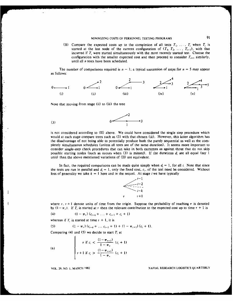
MINIMIZING COSTS OF PERSONNEL TESTING PROGRAMS 91
(II) Compare the expected costs up to the completion of all tests T 1 .... T when T, isstarted at the last node of the current configuration of (TI, T2,. .... T ,-_1), with thatincurred if T were started simultaneously with the most recently started test. Choose theconfiguration with the smaller expected cost and then proceed to consider T+1 similarly,until all n tests have been scheduled.
The number of comparisons required is n - 1; a typical succession of steps for n = 5 may appearas follows:
2 4 42 "- 3 3 5
0 . - - - 1 0 1 01 33i) 6 0i (iii) (iv ) (V )
Note that moving from stage (ii) to (iii) the tree
2
(3) 0 - -3
is not considered according to (II) above. We could have considered the single step procedure whichwould at each stage compare trees such as (3) with that chosen (iii). However, this latter algorithm hasthe disadvantage of not being able to potentially produce both the purely sequential as well as the com-pletely simultaneous schedules (unless all tests are of the same duration). It seems more important toconsider single-step check procedures that can take in both extremes as against those that do not skippossible starting nodes (such as occurs when (3) is missed). If the durations d are all equal (say 1unit) then the above mentioned variations of (II) are equivalent.
In fact, the required comparisons can be made quite simply when d = 1, for all i. Note that sincethe tests are run in parallel and d = 1, only the fixed cost, ci, of the test need be considered. Withoutloss of generality we take k = 1 here and in the sequel. At stage i we have typically
i-2-I
i-k
by 1 -rT) If i strte atr t en he ele an onrib to ot ee p ce c slpt i er +1iwhere T, T + 1 denote units of time from the origin. Suppose the probability of reaching T is denotedby (I - 7r,). If T is started at 7 then the relevant contribution to the expected cost up to time T + 1 is(4) (1 - 7r,) (ci- k + . + ci- I + Ci + 1whereas if T, is started at time r + 1, it is
(5) (1 - 7r,) (Ci k+ .. . c--I + 1) + (I - 7 1+ ) (c, + I).
Comparing (4) and (5) we decide to start T, at
rifc,< -1) (c, + 1)I - 7r",
r+lif c, > 0(r,) + )
VOL. 29, NO. 1. MARCH '982 NAVAL RESEARCH LOGISTICS QUARTERLY
92 P. D. FEIGIN AND G. H. HAREL
1 - '~where, clearly, 1 = (1 - .-.." (1 '-p -
For this situation we see that the comparisons can be made quickly and sequentially with aminimum of data to be stored.
The systematic application of the algorithm when the d are different will now be described. Sup-pose we are at stage i and wish to determine where to start test T. Suppose that X denotes the time ofthe last node so far and v the time of the most recent start (i.e., the time at which T,_ is commenced).Define the following quantities:
C - expected cost up to time A (T, excluded);
C - expected cost up to time P"
r - number of tests commencing at v (including T;);
s - number of tests commencing or in progress at time v;
V1, V2 . . . . . vs - indices of test commencing or in progress at time v;
R, < R2 < ... < Rs - time left to completion of tests v. vs, respectively-
K = ci_,+ - fixed costs of starts at time v;j-I
I - i', - probability of getting through all tests up until time P.
Note that the index i is among the indices v . vs.
Now if T is started at time X then the new expected cost is
(7) C = C + 01 -(1-pj) (c, + d)
with the remainder of the updating as follows:
X'=X + di, v'=X, C'= C,, r'= s'= 2, {vj', v') = (i, +1},
R' = min (d, d,+1), R = max (d, d+,), K'= ci + c,+,,
1- = I-I (I - pj).j-I
If T, is started at time X then the new expected cost is
(8) CA=C,,+(1-7r,)(K +p IR+(1- p,)I,,2 R 2 + ... + (I-pX (... (-p,,_)R }
with the appropriate updating determined by:
X'=v+R, v'=v, C,'= C, r'= r + 1, s'= s + 1, K'= K + ci+,, 7r.'= 7r,
and d,+1 being inserted into its correct place among R1. R, to give the new indices v1'. vI+Iand residual times R'. Rs+, .
At each stage i the smaller of (7) and (8) determines the appropriate scheduling of T and theappropriate updated quantities to proceed to the next stage.
NAVAL RESEARCH LOGISTICS QUARTERLY VOL. 29, NO. 1, MARCH 1982
MINIMIZING COSTS OF PERSONNEL TESTING PROGRAMS 93
C. Multistep Check Algorithms
At the expense of considerably increased computational effort the single-step check algorithm canbe extended by considering starting test T at several nodes in the existing configuration at stage i.There are at most i possible starting nodes so that if each one of these was investigated at each stage i,at most n (n + 1)/2 different configurations would be considered.
For example, one might start by considering a two-step check procedure which would involvecomparing the merit of starting, at stage i, T, at either the last node or one of the last two starting times.The algorithm would require storing considerably more information at each stage. However, there is noguarantee that the final schedule will be superior to that produced by the single-step check procedure.
Indeed, due to the serious interactive effect of parallel tests on the cost structure, it is not possibleto conclude that any multistep procedure will always do better than a one-step procedure. This isbecause on adding Tn, we may be better off with some Ti starting at a node determined by the one-stepprocedure than at the node to which it was allocated at stage i by the multistep procedure.
We therefore do not look further at the multistep check algorithms in this paper, although theiraccurate description still poses an interesting and possibly important problem.
4. NUMERICAL EXAMPLES
EXAMPLE 1.
Data: n = 3
i c1 di pi a, ai/Pi1 1 1 .25 2 82 8 1 .7 9 90/73 2 1 .2 3 15
ALGORITHM: We note that di = 1; i =1, 2, 3 so that we may use the criterion (6) at each
stage.
(1) Starting order is 1, 2, 3.
(2) Start T2 at 0 if c2 < (I - pI) (c2 + 1) - (.75)(9) = 6.75.
Hence, we start T2 at time I and the configuration stands as
0 1 2
(3) Start T3 at node I if c 3 < (I -P2) (c 3 + 1) = (.3) (3) = .9.
Hence, we start T3 at node 2 and the final configuration is
1 2 3
with total expected cost 9.425
VOL. 29, NO. I, MARCH 1982 NAVAL RESEARCH LOGISTICS QUARTERLY

94 P. D. FEIGIN AND G. H. HAREL
The optimal configuration is actually
0 2
_<3
with a total expected cost of 9.4. We note that a two-step check procedure would have given us thisconfiguration but that the one-step algorithm gives a very nearly optimal schedule. Here we also havean example of a case for which the optimal parallel testing schedule involves inversions of the testingorder for a sequential schedule (viz. starting T 2 on the completion of T3).
EXAMPLE 2.
Data: n - 3
i c, d, pi a a,/p
1 1 1 .3 2 20/32 4 3 .6 7 35/33 1 2 .2 3 15
ALGORITHM: We use the algorithm outlined by equations (7) and (8). The initial order isaJain 1, 2, 3, so that stage (1) consists of starting T, at 0. We now tabulate the relevant quantitiesdefined in the previous section for stages (2) and (3), explaining the calculations below.
k v r s Ivj} (R,) K 1-r, C CA
(2) 1 0 2 2 1, 2 1, 3 5 1 0 2(3) 4 1 2 2 3, 2 2, 3 5 .7 2 6.9
Stage 2: According to (7) C), = 2 + (.7)7 = 6.9
According to (8) Ck = 0+ (1)15 + (.3) 1 + .7(3))= 7.4
We therefore update according to equation (7).
Stage 3: According to (7) C; = 6.9 + (.7) (.4) (3) = 7.74
According to (8) CA - 2 + (.7) (5 + (.2) 2+ (.8) 3) 7.46
We do not need to update the quantities further. The tree has developed as follows:
/3
0 1 01 2 0 1 2
(1) (2) (3)
The algorithmi does produce the optimal configuration in this case, with total expected cost 7.46.
CONCLUSION
We have proposed an approach to personnel test sequencing which is based on cost effectivenessrather than predictive ability. Once a company has decided on which tests are required to determine job
NAVAL RESEARCH LOGISTICS QUARTERLY VOL. 29, NO. 1, MARCH 1982
MINIMIZING COSTS OF PERSONNEL TESTING PROGRAMS 95
suitability, then their application may be done more efficiently by considering the sequencing algorithmsdiscussed above.
It is clear that a major area of application lies in recruiting foi ,pecialized jobs in the governmentor the armed forces. Here, investigating the various facets such as security, health, intelligence andpersonality typically involve high cost and delays. Moreover, information is commonly available on thea priori probability that an applicant will meet the required standards in each area. We suggest that theideas presented here will help make the screening of applicants more efficient, either by implementingthe algorithms herein described or by encouraging the development of related ones.
REFERENCES
[1] Baker, K.R., Introduction to Sequencing and Scheduling (John Wiley and Sons, New York, 1974).12] Beach, D.S., Personnel: The Management of People at Work (MacMillan Publishing Co., New York,
1975).(3] Cronbach, L.J. and C.C. Gleser, Psychological Tests and Personnel Decisions (University of Illinois
Press, Urbana, 1957).[4] Dannenbring, D.C., "Estimating Optimal Solutions for Large Combinatorial Problems," Manage-
ment Science, 23, 1273-1283 (1977).[51 Harary, F., A Seminar on Graph Theory (Holt, Rinehardt and Winston, New York, 1967).
VOL. 29, NO. I. MARCH 1982 NAVAL RESEARCH LOGISTICS ,.UARTERLY
THE VARIANCE OF THE COVERAGE OF A RANDOMLYLOCATED AREA TARGET BY A SALVO OF WEAPONS
Gerhard Schroeter
Industrieanlagen-Betriebsgesellschaft mbHOttobrunn, Germany
ABSTRACT
We derive formulas for the variance of that proportion of the value of a ran-domly located, circularly symmetric area target that is destroyed by N indepen-dently fired weapons of identical typc whose damage functions are circularlysymmetric about the respective impact points. The probability density func-tions of the target center location and of the weapon impact points are also cir-cularly symmetric. The general results are specialized to uniform and Gaussianfunctions. In the latter case a closed-form solution (triple integral) for the vari-ance of the coverage is derived. Similar to some well-known results on expect-ed coverage, this expression for the variance of the coverage can be easilyevaluated by numerical quadrature. Numerical results are given which indicatethe target coverage variability caused by the combined effects of randomtarget-locating errors and weapon impact point fluctuations.
INTRODUCTION
Two-dimensional coverage problems arise frequently when assessing the effectiveness of artilleryor air-to-ground weapons. The surveying papers of Eckler [51, Eckler and Burr [6], Guenther and Ter-ragno [161 show that there are many papers concerned with the expected coverage of an area target by
multiple independently fired weapons. This reflects the importance of knowing the averageeffectiveness of weapon systems. However, in military requirements another criterion is often used:The measure of effectiveness for a salvo of N rounds is the proportion E of the total value of an areatarget that is destroyed with a probability of at least y. Expected coverage, obviously, does not supplysuch information, even though, of course, a higher expectation of destroyed value generally increasesthe confidence level y for any given E (or vice versa). What would be required in the case of an c-y-criterion is not only the expectation of the destroyed value or coverage, but the distribution of the cov-erage. In sharp contrast to the bulk of papers on expected coverage, only very little literature is avail-able on the distribution problem. Domb [41, Siegel [341 and Votaw [38] have calculated distributionsof the coverage for arbitrary numbers of covering objects N >, 1, they, however, treat only one-dimensional coverage problems (line segments and circular arcs), and their methods do not seem appli-cable to area problems. Solomon [35] derives in two dimensions the distribution of the destroyed valueof an area target by one weapon only and gives some upper and lower bounds for y (given f) in thecase of two weapons. Several authors have derived expressions for the higher moments (especially thesecond moment) of that fraction of a fixed geometrical target figure or body which is covered by N ran-domly thrown figures or bodies (Ailam [IW, Bronowski and Neyman 121, Garwood [131, Greenberg[151, Moran and Fazekas de St. Groth 1241, Robbins [251 and [261, Santal6 [271). The principal resultobtained in this connection is due to Robbins [251. Others (Cooke [31, Edens [7], Flatto 18], Flattoand Konheim [91, Flatto and Newman [10], Gilbert [14]. Hoist [181 and [191, Kapian [201 artd [2!],Miles [231, Shepp [321, Siegel (331, Steutel [361, S12vens [371) estimate the probability :hat therandomly thrown figures cover the fixed target figure completely, or estimate the number of figuresrequired to cover the target figure completely.
VOL 29, NO 1, MARCH 1982 97 NAVAL RESEARCH LOGISTICS QUARTERLY
~GJ.1~O PAaE B hM(ii0T niLI6

A11IIIIIIIIIIAD-Au G OFCE OF NAVAL RESEARCH ARLINGTON VA FIG 15/5
MAYIIAIIIIIIIWILSIID MAR 82NAVAL RESEARCH LOGISTICS QUARTERLY. VOLUME 29. NUMBER 1.1W N
22 flllfffflll
mEEEEIIEEEEIIEEIhIIIEEI E
INIE EEDhE h7EEEE-EEh
98 G, SCHROETER
From all these results, those on the second moment of the coverage in the space of two or moredimensions are the most interesting with respect to weapon analyses. Although the second moment (orthe variance) does not supply the precise information that is required for the E-y-criterion, it isnevertheless useful, since Tchebyshev's inequality can in some cases yield a lower bound for e (giveny) or y (given 0). The papers cited, however, are confined to one situation; this limitation resultspartly from modeling the coverage problem as an overlap-of-geometrical-figures problem. In weaponanalyses terms, it is: (1) The only targets considered are those with sharp edges and uniform value den-sity. (2) The only weapons (randomly thrown figures) are those with zero-one damage functions; com-plete destruction occurs within the weapon effects area, and no destruction without. (3) The weaponimpact points are assumed to be distributed uniformly within a specified area. For most applications,these three assumptions could be accepted as more or less good approximations of the real world.However, one limitation is a serious drawback, which reduces the usefulness of the former results onthe variance of the coverage: (4) The target position is not a random variable, or in our words: The tar-get location error is zero with probability one.
It is the objective of this paper to derive expressions for the variance of the coverage in more gen-eral situations so that limitations (1) to (4) are eliminated. First, we generalize Robbins's [25] mainresult on the moments of the coverage of geometrical figures to randomly located targets with generalvalue density function. Second, we consider a coverage problem in which all underlying functions areGaussian, and derive a closed-form solution (triple integral) for the variance of the coverage. In thisGaussian case the standard deviation of the coverage can be determined in little computer time bynumerical quadrature so that a parametric analysis can be made. Numerical results will be presentedwhich clearly indicate the variability of target coverage caused by the combined effects of randomweapon impact point and target location fluctuations. As a side result, we generalize a formula of Gar-wood 113] and Santal6 [271 for the variance of the coverage of one circle by N other circles.
The concepts of the Gaussian target and the Gaussian damage function have been considered inmany papers (see, e.g., Fraser I II] and 112], Eckler 15], Eckler and Burr 161), dealing with problems onexpected coverage; the main advantage of this model-beyond its intuitive appeal as an approximationof real world situations-is that many problem solutions can be given in closed form which is not possi-ble when corresponding problems with other functions are considered. This same property will ulti-mately be used to derive the triple integral expression for the variance of the coverage of the normallylocated Gaussian target by warheads with Gaussian damage functions and normally distributed impactpoints.
1. THE COVERAGE PROBLEM
Target Value and Location Distribution
We consider-on an x-y-plane, where x, y are Cartesian coordinates-a circularly symmetric areatarget whose precise position is not known because of a random locating error (see Figure 1). Weassume that the probability density function (p.d.f.) .fA (XT, YT) of the coordinates of its center isknown, and that fA (XT. YT) is circularly symmetric with respect to the origin 0 of the x-y-coordinatesystem, so that fA (XT, .Y) = f[(xT + y)"12]. The point 0 is the expected target center location.
The area target value need not have a uniform density; for many applications it has proven usefulto consider the concept of a nonuniform target value density function w4 (u, v) as done, for example,by Eckler [51, Eckler and Burr [61, Helgert (171, McNolty [22J, Schroeter 1281, 1291, 1301, 1311, andWashburn 1391. The function WA(U, v) need not be greater than or equal to zero, although in theusual applications it is. Our following results will apply to any value density function that is absolutelyintegrable over the u-v-plane, and circularly symmetric with respect to the center T of the target, so
that wA (u, v) = wf(u2 + v2)1/ 2) within a u-v-coordinate system whose origin is at T.
NAVAL RESEARCH LOGISTICS QUARTERLY VOL. 29., NO. 1, MARCH 1982

VARIANCE OF RANDOMLY LOCATED AREA TARGET COVERAGE 99
vi
Ii
TARGET
--- COVERED TARGET AREA
F(GURE I Coverage of circular target by 4 'cookie-cutter' rounds
P.D.F. of Impact Points of Weapons
In the following we consider a salvo of N identical rounds. We assume that the weapons areaimed at the origin 0 of the x-y-plane, the expected location of the target center. (Aiming all weaponsat that point will not necessarily maximize the expected target value destroyed.) Because of randomdelivery errors, however, the weapons will not impact at 0, but at points 1,(x,, y 1), j = 1 .... ,more or less dispersed around 0. We consider the set of impact points as a sample, randomly andindependently drawn from a population with the known p.d.f. kA(x, Y) which is circularly symmetricand centered at 0, so that kA(x, y) = k[(x2 + y 2 )1/ 2].
Damage Function of Weapon and Coverage of Area Target
We introduce a Cartesian f -- coordinate system whose origin is at the impact point of a weapon.We assume that the effectiveness of the weapon can be adequately described by a circularly symmetricdamage function dA(f, 7)) = d[(q2 + q2)1/21, with 0 < dA (f, .O) < 1. This function has the followinginterpretation: The value of that element of an area target which lies at the point with the coordinatesf, q is reduced by the factor I - d (f, -q). This implies that the value density of the target remainingafter the bombardment by the weapon is WA"(u, v) = w4(u, v) [I - d4 (u - f., v - "or)], wherein
f, TIr are the target center coordinates in the f - "o-coordinate system, or the weapon impact pointcoordinates in the u-v-coordinate system whose origin is at the target center. (This property alsoapplies to any noncircularly symmetric functions wA and dA, if only the axes of the u-v-and the ,-9-coordinate systems are respectively parallel. The superscript in parentheses indicates the number ofweapons considered.) Hence, the total destroyed value (or coverage) C('(T , TIT) is the followingfunctional of WA and dA:
=C~'1 (QT, 'IT) = w, (u, v)dA(u - v - 7. )dudv
= f_ f -A r) - A (f7) d dqo,
This is the two-dimensional convolution of the two functions w4 (u, v) and d,(-., -i), orw4 (-u, -v) and d4 (f, I).
VOL. 29. NO. I, MARCH 1982 NAVAL RESEARCH LOGISTICS QUARTERLY

100 G. SCHROETER
If both, wA and d4 are the "cookie-cutter" functions for the two geometric figures 'and .9,respectively, (i.e., when they equal one within ' and d, respectively, and zero without), thenC tt ("r, 'oT) is the intersecting area of V'and -. This is, of course, the usual definition of the cover-age of one geometric figure by another. Using (1), one can immediately generalize this concept tomore general targets and damage functions, and this definition has been applied in all papers wherenonuniformly-valued area targets have been considered.
Coverage of Area Target by Multiple Weapons
Remember that the target center and weapon impact points coordinates in the x-y-coordinate sys-tem are xr, Yr, xi, Yi ...... r, Yv, respectively. The coverage of the target by all the N weapons thenis the following function (cf. Schroeter [311, Equation (6)):
(2a) C('V(xr, Yr, X 1, Y1. . ,vy = K- f . . w(X-XT, Y-VT) I[-dA (x-x,, r-y)ldxd,
wherein K is the total value of the target, K = f- f 4 (u, v)dudv = 2rf w(t)t d. Define
C = C" ) and denote the not-destroyed value K-C by C. (The complement of the destroyed value orcoverage is sometimes termed "vacancy" (Ailam 11], Hoist [18])). Define d 4 (t, -9) = d[(f 2 + q2)1/2]
1- d4(,, ). Then
(2b) (x, YT, X, Y1, . . XN, YN)=ffwA (xxr.--Y)f 4 (X Y ,)dxdv.
Considering the target center and weapon impact point coordinates as random variables, we will deter-mine the variance of C, which is the same as the variance of C.
Coverage of Area Target and Probability of Killing a Point Target
In this paper, we will not go deeper into the analysis of point targets, It is, however, interestingto relate the concept of the coverage of an area target with the probability of killing a point target, sincethis will enable us to generalize, in Section 2, a theorem of Robbins 1251 on the relation between themoments of the not-destroyed value of the area target and the probability of killing none of severalpoint targets. This theorem has been applied by several authors to calculating the second moment ofthe coverage (as done, for example, by Garwood [131).
Consider a point target which will either survive an attack by a weapon or be killed. Defined4 (f, 7) to be the conditional probability of killing the point target provided it has the coordinates , r1in the coordinate system whose origin is at the weapon impact point. If the point target is located ran-domly round the point T( r, TT) according to the probability density function WA(u, v), thenC"'(fr, "qr) as defined by (1) is the unconditional probability of killing the point target. (This proba-bility is unconditional with respect to the random location of the point target round T, it is a conditional .probability with respect to the location of T itself.) Evidently, C(N) = C as defined by (2a) equallyyields the probability of the randomly located point target being killed by at least one round of thesalvo. Hence, the concepts of coverage of area target and probability of kill of point target areequivalent, when dA is interpreted in the dual form, as done above, against point and area targets.Also, when xT, YT, X1, .Y1. XN, YN are considered as random variables, then the expectation Ec ofthe destroyed value of the area target equals the totally unconditional probability of killing the point tar-get. This equivalence is well-known (see, e.g., McNolty [22], Schroeter [28] and [31]).
I am indebted to the referee for having pointed out the following interpretation: Let X denote anindicator variable for the kill of the point target, i.e., X = 1, whenever the point target is killed, andX = 0 otherwise. Again, let wA(u, v) be a probability density function. Then C"',I = C from (1) and(2a) equals the conditional expectation of X. Similarly, E- equals the unconditional expectation of X,
NAVAL RESEARCH LOGISTICS QUARTERLY VOL. 29. NO. I. MARCH 1982

VARIANCE OF RANDOMLY LOCATED AREA TARGET COVERAGE 101
" Ex. Since X is either 0 or 1, its distribution is completely known whenever Ex is. Especially, the vari-ance of X, o-x2, equals Ex(l - Ex). Thus, nothing would remain to say on the variance of the coverageif such were the problem to be analyzed in the present paper. Instead, what we are addressing could bedescribed, somewhat loosely, as a target consisting of an infinite number of point targets, their fre-quency round T being proportionate to the density function wA (u, v), and C) from (1) and (2a)denoting the fraction killed. The variance of that fraction, o', generally is less than EC(l - Er).
2. MOMENTS OF NOT-DESTROYED VALUE
The mth Moment of the Not-Destroyed Value
The mth moment of the not-destroyed value C is
(3a) E ~f_ f Nd xx, y dxdyf WA (X XT, Y Yd 1 i- ( X
j-1
N
fA (XT, Yd) H kA (Xi, Y, )dXT dYT dX I dyI ... dX dj-1
We write the mth power of the inner double integral with respect to x, y as a repeated 2m-fold integraland interchange the order of the integrations. This is allowed since the integrand is an absolutelyintegrable function of each of its arguments. Thus, we obtain
i-I J-f I-I
dxIdyI ... dXNdYNdXTdYTdfidih ... d. d7)j.
The inner repeated integral with respect to xj, y. xN, YN may now be written as the Nth powerof a double integral, so that(3b) Ee--=f -f f YT) M XT, 11i (Y,)
i-I
kA ( , rl _ d. ( ,f, O,-'l~d d'r Xrdyrdfi d-qj ... d ,,d7),,IfI-I
The integral of fA (XT, Y) JJ WA ( , - XT, h - YT) with respect to XT, Yr is completely analogous toi-I
the integral of kA (f, ij) ldA ( , -Q , " - q) with respect to f, 7). This suggests the following func-
tional be defined:
(4) Om (f1,iq, ). m, 7)m;k,, d) =ff k, (f, q)) rld - ri--)d~d-I- I
which implies
(5) f' f fA(XT, Yr) W. ,(f, - XT, 7 - Yr)drdYr = OQ(, , 1)]. f,,7)m; fA, WA).1-1
Using (4) and (5) we obtain for the mth moment of the not-destroyed value as an alternative form of(3b):
3c) Eem - . m q. _q... A. WA)
.. N. (f, 7.1..... i)m,, kA, dA)d Id7jI ... dfmdTI.
VOL. 29, NO. 1, MARCH 1982 NAVAL RESEARCH LOGISTICS QUARTERLY
102 G. SCHROETER
This shows that Ee, is an integral of a product, whose second factor is independent of the target value
density function and the target location error p.d.f.; this factor contains all information on the weaponsand on the p.d.f. of their impact points. The first factor contains all information on the target and itslocation error, and is independent of damage functions and impact point p.d.f.'s.
The usefulness of (3b) in contradistinction to (3a) will become apparent when we consider thesecond moment, at the same time taking into account that, in real situations, the number of weapons Nfired in a salvo generally is much greater than 2. Both, in (3a) and in (3b), the inner integrals are dou-ble integrals- the outer integrals are (2N + 2)-fold in (3a) and (2m + 2)-fold in (3b). For N > m,therefore, a reduction of the number of integration processes is possible by using (3b) instead of (3a).
Interpretation of the Functional Q,.
For m > 1, 0, does not satisfy the commutative and associative laws for its argument functions,such as the ordinary convolution does. It has. however, a statistical interpretation similar to that of theconvolution: Let wA(6, -q) and fA(x, y) be two p.d.f.'s. Then ,(f , )1 .... ,,,, 1,,; fA, wA ) is thejoint p.d.f. of the coordinates f,, ij of m points B,, i = 1 ... m , which are located randomly andindependently according to the p.d.f. wA around a common center T which, for its part, is drawn ran-domly from the x-y-plane according to the p.d.f. f, (x, y). Another interpretation results from (2b);evidently
C(xT Yr, X1, Y. XN, YN) = QN(XT - X 1, YT -Y . XT - XN, YT - YN; WA, dA).
Robbins's Theorem
An examination of (4) will show that Qm( i, "h. m' 'urn; kA, dA) is the probability of killingnone of m different point targets, located at the points B,(, -), by a single round whose damage func-tion is dA and whose impact point p.d.f. is kA(, "0). Hence, m . m, ,im; kA, dA) is theprobability of killing none of these point targets by a salvo of N identical and independent rounds.Interpreting, as in the section before, 0,(f, 71 .... ,, t.re fA w,) as a joint p.d.f., we see from(3c) that the mth moment of the not-destroyed value of the area target, EZ,, equals the unconditionalprobability of killing none of m randomly located point targets-which are distributed according to thep.d.f. WA round the common randomly located center T-with the salvo of N rounds. This is the gen-eralization of Robbins's 1251 result on the moments of the coverage of a fixed geometrical figure byrandomly thrown figures to the coverage of a randomly located target with arbitrary value density func-tion by weapons with general damage functions. Evidently, these results equally apply to coverageproblems where the underlying functions are not circularly symmetric.
Expressions for the Second MomentBecause of the assumed circular symmetry of wA, f. d, and kA, the integrals
Q2fl. 11, 2,, kA, j,4) - w 'R)dA (f1 - f, -- '1) dA (f2 - _ q12 - 71) df d,
depend only on the relative positions of the three points 0(0, 0), 81(f, 711), and B 2(f 2 , 172). There-fore we may, without loss of gen-ality, express them in terms of the three parameters i, t2, 0 whosegeometrical interpretation is indicated in Figure 2. A routine manipulation then yields for the secondmoment of the not-destroyed value:
(6) - 27 Ja J J2 - Q t2(. 12- f, w)Q2V(tl, 12, 0;k, d) t1 t2dOdt1 dt -,
NAVAL RESEARCH LOGISTICS QUARTERLY VOL, 29, NO. I, MARCH 1982
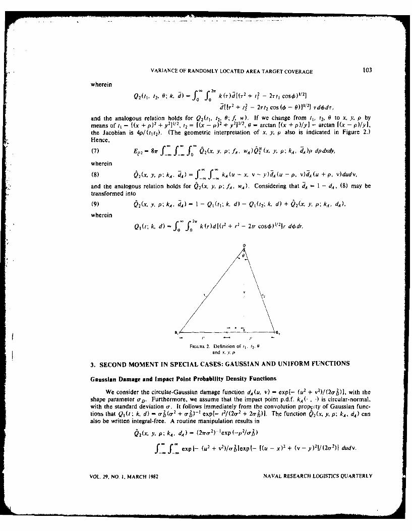
VARIANCE OF RANDOMLY LOCATED AREA TARGET COVERAGE 103
wherein
, 1 , 02; k, ) = fo 2v k(T)d[&2 + t2 - 2Tt, cosO)112 ]
d[7 2 + t2 - 27t2 cos ( - 0)]2 } rd) dr,
and the analogous relation holds for Q2(ti, t2, 9; f, w). If we change from 11, t2, 0 to x, y, p bymeans of tj = f(x + p)2 + y21112, t2 = (x - p) 2 + y2]11 2, 9 = arctan (x + p)/y] - arctan I(x - p)/yl,the Jacobian is 4p/(tit2). (The geometric interpretation of x, y, p also is indicated in Figure 2.)Hence,
-0
-.0 - 02 (X -P A . 2 X ,P A pd xy
(7) Ec 2 = 8r JJ f2xy~~A wAQ(xypo dA)dd~Y
wherein
(8) 0 2(x, y ,P; k, , d f f kA( - x. v- y)dA(u - p, v)dA(u + p, v)dudv,
and the analogous relation holds for 0 2(x, Y, P; fA, WA). Considering that ds - 1 - dA, (8) may betransformed into
(9) 2(x, y, p; kA, dA) = I - Q1(1; k, d) - Q1(12; k, d) + 0 2(x, Y, p; kA, dA),
wherein
Q(t; k, d) =: fo k(r)d[(t2 + r 2 - 2tr cos0)'I/2 ]r d0dr.
0
V
B" 6
FIGURE 2. Definition of it. r2.and x, y. p
3. SECOND MOMENT IN SPECIAL CASES: GAUSSIAN AND UNIFORM FUNCTIONS
Gaussian Damage and Impact Point Probability Density Functions
We consider the circular-Gaussian damage function dA (u, v) - exp[- (u2 + v2)/(2o-)], with theshape parameter oD. Furthermore, we assume that the impact point p.d.f. kA ( , ) is circular-normal,with the standard deviation a-. It follows immediately from the convolution property of Gaussian func-tions that Q1(t; k, d) - o',(o2 + o')-' exp(- t2/(2o 2 + 2aoj)]. The function Q2(x, y, p; kA, ds) canalso be written integral-free. A routine manipulation results in
Q2(x, Y, P; kA, dA) = (27r0a2)-'exp(-p 2/0.2D)
f. f exp i- (u 2 + v2)/rlexp{2- [(u - x) 2 + (v - y) 21/(2(71)) dudv.
VOL. 29, NO. I, MARCH 1982 NAVAL RESEARCH LOGISTICS QUARTERLY

104 G. SCHROETER
We recognize the double integral as the two-dimensional convolution of two Gaussian functions, sothat this integral can be expressed as a Gaussian function of x and y. Consequently:(10) Q2 (x, Y, P k'A, dA) = 0
2(2
0 2 + 0)-exp[-_p2/O 2 - (X
2 +y
2)/(2
0 2 + o°2)1.
Gaussian Target Value and Location Probability Density Functions
For a Gaussian target with the total value of one and the shape parameter oaz , we haveWA(u, v) = (2r'0z)-texp- (u2 + v2)/(2Mj)]. Let the p.d.f. of the coordinates of its center becircular-normal, with the standard deviation 00T. Then, quite similar to the above case,Q(t; f w) = [21T(0 2 + a-2)1-'expf-t 2 /(2o- 2 + 20-2)] and
(11) 6 2(x, Y, P;fA, wA) = [47F20 2 (202 + 02 )]-|exp[-p 2/0 1- (x2 -ry 2)/(202 + 0j)].
Combining these value density and location p.d.f.'s with the Gaussian damage functions and the normalimpact point p.d.f. will, for the expectation of the not-destroyed value, yield
22 + 0_2_-_ lidt(12) Ec = (- + o-z) exp 2(-2 + 0-2)1 i 2 + o.2 exp 2(o.2 + o-2) t at.
Observing (9) and inserting (10) and (11) into (7) will, for the second moment of the not-destroyedvalue, yield a triple integral with respect to x, y, p. Then, a change to polar coordinates by x = r cosk,y = r sinO will finally result in
f 8/ 2 o exp p2 cs r cos
2( 202 +2 j 2(.02 +02) 2o 2 + 02
N
+ 2002 exp -2 22 + 02 IFd drdp.+"D I- (D 2a- +D JJ i
The integrals (12) and (13) can be solved in closed form, by developing the Nth powers and integratingthe sums term by term. Practically, this is of little interest, since the complexity of the integrands isprohibitive for large N. (12) and (13), however, can be computed easily by numerical quadrature forarbitrary values of N.
Coverage of Fixed Circle by Randomly Thrown Circles
In this section we apply our main result of Section 2 to generalizing results on a circularly sym-metric coverage problem considered by Garwood 131 and Santal6 1271. These authors calculated thesecond moment of the coverage of a fixed circle (radius Rr) by N identical, randomly thrown circles(radius a) when the centers of the latter are distributed uniformly over a circle with radius RD. Thecenters of the two circles with the radii RT and RD coincide.
The damage function d(r), in this case, is 1 if T < a, and 0 else. We denote by kA (u, v) theuniform p.d.f. over the circle with the radius RD. Then 7rR2Q,(t; k, d) is the intersecting areaS, (; RD, a) of the two circles with the radii a and RD whose centers are the distance t apart. Further-more, 7rR2Q 2(,, t2, 0, k, d) is the intersecting area of the three circles with the radii RD, a, a, and
NAVAL RESEARCH LOGISTICS QUARTERLY VOL. 29, NO. I, MARCH 1982
VARIANCE OF RANDOMLY LOCATED AREA TARGET COVERAGE 105
the centers at the corners 0, B1 , B 2, respectively, of the triangle indicated in Fig. 2. We denote this
intersecting area of the three circles mentioned by S 2(t1, 12, 0; RD, a) and, using (9), obtain
(14) Q2(ti, t2, 0; k, d) = I - ('R2)-[S1 (tj; RD, a) + S 1(12; RD, a) - S 2(,1 , t2' , RD, a)f.
Next we consider the target whose value density is one within a circle of radius Rr, and zero without.
We assume that this target is centered, with the probability one, at the point 0(0, 0). In this case
Q2(1t, t2, 0; f, w) = 1 if ti < RT and f2 < Rr, and 0 otherwise. Hence (6) yields
EZ2 = 2r f 0 fo fo Q7 (2' 12, 0; k, d)t 1t2dod,,dt2.
Combining this with (14) results in the second moment for that proportion of the fixed circle which is
not covered by the N randomly thrown circles of radius a:
(15) E 2=tr ff f 0 Lr {1- (1TR~)-[SI(1 ; RD , a) + S1 (12; RD, a)
- S 2(t1 , t2, 0; RD , a)]},t 1 t2dOdtjdt2.
This is the generalization to arbitrary relations of Rr, RD, and a, of results of Garwood and Santal6,
who considered only the case RD - a >, Rr. In the latter case, (15) may be reduced to a one-fold
integral; a short manipulation results in
EZ2 = 27r fr S1 (z; Rr, RT)M1 - (7rRY0 127ra 2 - S1 (z; a, a)]l}'zdz,
which is an alternative form of Garwood's Equation (43) and Santal6's Equation (5.3).
4. NUMERICAL RESULTS FOR GAUSSIAN FUNCTIONS
Equations (12) and (13) were evaluated by numerical integration, and the standard deviation or,
of the destroyed value was determined by means of the relation o-= 2 7 = - (E-) 2. In all cases
we assumed oaz = I. Figure 3-6 show in the Ec-oy(.-plane the two families of parameter curves
o- - const. and N = const. for o'D = 0.1 and 0.2, o- = I and 3. Many practically important cases fall
within the range of these parameters.
Discussion of Results
The figures indicate that, for ('T < 1, the standard deviation of the coverage is so small that the
one-sided Tchebyshev inequality P(Ec - ac- < C) >, a2/(I + a 2) may be well applied to deriving a
confidence level for the minimum destroyed value. Take, e.g., o'D = 0.1, (r = 1, (TT = 0.5, N = 250
rounds. It can be seen in Figure 3 that Ec 57%, oc- :- 5%, so that the coverage is with a probability
of at least 90% greater than 42%. For O'r >> 1, however, Tchebyshev's inequality will be of little
value for our problem.
We see that, for increasing r T and N, the standard deviation of the coverage 0r - approaches its
theoretical upper bound on the circle with the equation oc = E((1 - E(.). This circle is drawn as a
dashed line. This property implies that the probability mass concentrates more and more near C = 0and C - 1.
Numerical Method
The integrals (12) and (13) were evaluated by a Gauss-Legendre quadrature. For (13), generally
243 supporting points were used. For special values of the parameters, 32- supporting points were
chosen. With a Fortran program, on a CDC 6500 computer approximately three seconds of central pro-
cessor time was required to determine one value of (T(. with 243 supporting points.
VOL. 29, NO. I, MARCH 1982 NAVAL RESEARCH LOGISTICS QUARTERLY

106 G. SCHROETER
0.5'
0.4-
2-0
c.)
4-
0 0.Exece Coerg 0E
2IUR 3.Sadr eito00cvrgev ~pce oeae~
NAVA REERHLGSIS UREL O.2, O MRH18
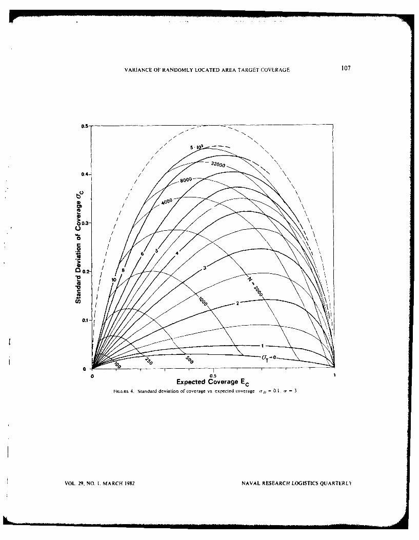
VARIANCE OF RANDOMLY LOCATED AREA TARGET COVERAGE 107
0.5-
0.4-
20
000
0
00.3
a.2 -
C
0 0.5Expected Coverage ECFIGURE 4. Standard deviation of coverage vs. expected coverage. (T 0.1. 3
VOL. 29. NO. 1, MARCH 1982 NAVAL RESEARCH LOGISTICS QUARTERI
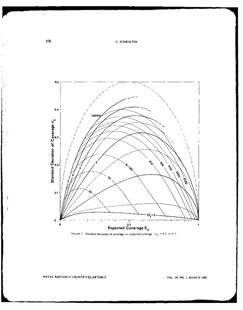
108 G. SCHROETER
0.5 --
0.4 / /128000
0
0
C.)2
0 0.5
ExpectedOr Coeae 0
F'tGLIRE 5. Standard deviation of coverage vs expected coverage ar1,) 0,2. (y I
NAVAL RESEARCH LOGISTICS QUARTERLY VOL. 29. NO. 1, MARCH 1982

VARIANCFr OF RANDOMLY LO('AIH) ARFA TARGET (:ONTRAGI: 109
128000 _
800
4-
-3]
0
0 05 1E.2tdCoeaeE
1 io 6 S~n~r c~Tno lCi Cp~~ )c~g ,~l
ACKNOLED(NIEN
Thi wokwsd2 o h iityo ~fns fteFdrlRpbi fGray
REE0NE
(11Alm . Mmnso oeaeadCvrg Sae. ora fApidPoaiiy ,50
555 (966)
02.rn1k.J n .Nya. TeVrac fteMaueofaToDmninlRno e.
131Cooe. .J "Bund fo CoeraEpoebtes Covthg E.piain oSqenilCvrg rblems," see , Stadar c81-293 (1974). sexetd i% rlg
11 Ailomb, C., "ThMole of raand Coerageo Sa," nel.'ppie Proednsobh ambridge.,Philo-
sophial ociatety. ca 43. itis 1294 3303947)95)
VOL 29. NO. 1. MA 'RCH 1982 NAVAL RESEARCH LOGiISTICS QUARTERLYN
110 G. SCHROETER
151 Eckler, A.R., "A Survey of Coverage Problems Associated with Point and Area Targets," Tech-nometrics, 11, 561-589 (1969).
161 Eckler, A.R. and S.A. Burr, Mathematical Models of Target Coverage and Missile Allocation, MilitaryOperations Research Society, Alexandria, VA (1972).
[71 Edens, E., "Random Covering of a Circle," Indagationes Mathematicae, 37, 373-384 (1975).[81 Flatto, L., "A Limit Theorem for Random Coverings of a Circle," Israel Journal of Mathematics,
15, 167-184 (1973).[91 Flatto, L. and A.G. Konheim, "The Random Division of an Interval and the Random Covering of
a Circle," SIAM Review, 4, 211-222 (1962).[101 Flatto, L. and D.J. Newman, "Random Coverings," Acta Mathematica, 138, 241-264 (1q77).[11 Fraser. D.A.S., "Generalized Hit Probabilities with a Gaussian Target." see [21. 22. 248-255
(1951).[12] Fraser, D.A.S., "Generalized Hit Probabilities with a Gaussian Target Ii," see (21, 24. 288-294
(1953).[131 Garwood, F., "The Variance of the Overlap of Geometrical Figures with Reference to a Bombing
Problem," Biometrika, 34, 1-17 (1947).[14] Gilbert, E.N., "The Probability of Covering a Sphere with N Circular Caps," Biometrika, 52, 323-
330 (1965).[15] Greenberg, ., "Th, Moments of Coverage of a Linear Set," see (I,. /7, 865-868 (1980).116] Guenther, W.C. and P.J. Terragno, "A Review of the Literature on a Class of Coverage Problems,"
see [21, 35, 232-260 (1964).[17] Helgert, H.J., "On the Computation of Hit Probability," Operations Research, 19. 668-684 (1971).[181 Hoist, L., "On Multiple Covering of a Circle with Random Arcs." see [1, 17, 284-290 (1980).[191 Hoist, L.. "On Cie Lengths of the Pieces of a Stick Broken at Random," see Il]. 17, 623-634
(1980).1201 Kapian, N., "Two Applications of a Poisson Approximation for Dependent Events." Annals of Pro-
bability. 5, 787-794 (1977).1211 Kaplan, N.. "A Limit Theorem for Random Coverings ofa Circle which Do Not Quite Cover." see
[11, 15, 443-446 (1978).[221 McNoltv, F., "Expected Coverage for Targets of Non-Uniform Density," Operations Research. 16,
1027-1040 (1968).[231 Miles, R.E., "The Asymptotic Values of Certain Coverage Probabilities," Biometrika, 56. 661-680
(1969).[241 Moran, P.A.P. and S. Fazekas De St. Groth, "Random Circles on a Sphere," Biometrika 49, 389-
396 (1962).1251 Robbins, H.E., "On the Measure of a Random Set," see 121, 15. 70-74 (1944).[261 Robbins, I.E., "On the Measure of a Random Set i," Annals of Mathematical Statistics. /6, 342-
347 (1945).[27] Santal6, L.A., "On the First Two Moments of the Measure of a Random Set." see [21, 1,. 37-49
(1947).[281 Schroeter, G., "Probability of Kill and Expected Destroyed Value if the Underlying Distributions
Are Rotationally Symmetric," Operations Research, 24, 586-591 (1976).[291 Schroeter, G., "The Application of a Hankel Transformation to a Class of Circularly Symmetric
Coverage Problems," Operations Research, 25, 675-687 (1977).[301 Schroeter, G., "The Application of the Hankel Transformation to Spherically Symmetric Coverage
Problems," Journal of Applied Probability, 17, 1121-1126 (1980).[311 Schroeter, G., "Expected Coverage of a Randomly Located Target by Multiple Independent Sal-
vos," Operations Research, 28, 1299-1318 (1980).[321 Shepp, L.A., "Covering the Circle with Random Arcs," Israel Journal of Mathematics, I1, 328-345
(1972).[331 Siegel, A.F., "Random Space Filling and Moments of Coverage in Geometrical Probability." see
(11, 15, 340-355 (1978).
NAVAL. RESEARCHl LOGISTICS QUARTERLY Vo 29, N) 1, MAR('I t182
VARIANCE OF RANDOMLY LOCATED AREA TARGET COVERAGE I1
1341 Siegel, A.F., "Random Arcs on the Circle," see (1], 15, 774-789 (1978).[351 Solomon, H., "Distribution of the Measure of a Random Two-Dimensional Set," Annals of
Mathematical Statistics, 24, 650-656 (1953).(361 Steutel, F.W., "Random Division of an Interval," Statistica Neerlandica, 21, 231-244 (1967).[371 Stevens, W.L., "Solution to a Geometrical Problem in Probability," Annals of Eugenics, London,
9, 315-320 (1939).[381 Votaw, Jr., D.F., "The Probability Distribution of the Measure of a Random Linear Set," Annals of
Mathematical Statistics, 17, 240-244 (1946).139] Washburn, A.R., "Upper and Lower Bounds for a Pattern Bombing Problem," Naval Research
Logistics Quarterly, 21, 705-713 (1974).
VOL. 29, NO. I, MARCH 1982 NAVAL RESEARCH LOGISTICS QUARTERLY
REFORMULATING ZERO-SUM GAMES
WITH MULTIPLE GOALS
Edward L. Hannan
Office of Health Systems ManagementNew York State Department of Health
Albany, New York
ABSTRACT
This paper investigates the two-person zero-sum multiple payoff game inwhich the objective is to minimize a player's total underachievement from afixed set of goals. It is demonstrated that a previous formulation of this prob-lem can be substantially simplified.
1. INTRODUCTION
In a previous paper in NRLQ, Cook [11 discussed the formulation and solution of a two-person,zero-sum game with multiple payoffs in which the objective is to minimize the total underachievementfrom a fixed set of goals for each of the objectives.
The resulting formulation is
(1) min /3-vE k,,
subject to
SxA,j(r) - 0 < 0 Vj,r;x E x
where player I selects strategy i with probability x,,
X- (x-, x 2. )
X - x=(xI, . .. Xm xi I, X' x 0 > V Oi}
K
(r) Xj lk,
k-l
AlA ~k).(gk ak~)
K is the number of objectives
J is the index for player 2's strategies
, is the goal for the kth objective
VOL. 29, NO i, MAR( If 1982 113 NAVAL RESEARCH LOGISTICS QUARTERLY
ffmsCDuIQ pMIKs BL.mOm IIuaD

114 E, L. HANNAN
a is the payoff for the kth objective corresponding to player I choosing strategy i and player
2 choosing strategy j
AY (r) is the ijth component of A (r)
a is the set of extreme points of tb
q, ,= (CI . ... k) 0<o ak< W1.
r = 1. R is the index on the extreme points of 0.
wk = the relative weight placed on the kth goal.
This is a linear programming problem. After calculating the A (r) matrices, the problem involvesthe minimization of a linear function subject to m ( 2K- 1) + 1 constraints where m is the number ofstrategies available to player 1 and K is the number of multiple payoffs. Also, the calculation of the 2KA (r) matrices prior to solving the problem can be quite time-consuming.
The intent of this paper is to demonstrate that the same problem can be solved by minimizing alinear function subject to n(K + 1) + 1 constraints, where n is the number of strategies available toplayer 2. Also, only K matrices must be calculated prior to the solution of the problem rather than 2K
matrices.
2. A NEW FORMULATION
Letting ak represent the kth payoff to player 1 if player I chooses strategy i with probability x,,
i=1,... m, and player 2 chooses strategy j, j = 1. n, it follows that ajx, is the kth payoff toIiI
player I for this combination of strategies.
Thus,
= ma=10x 1 -0, .- xJ
is the underachievement of goal k (gk) corresponding to this strategy combination.
But dj = max 10, (gk- a )xiIM
since gk is constant and X, = 1.i-i
Since each of these dk values are weighted by corresponding wA values, player I selects x,
[Xi >0, X = IJ which will yield
min max Y wkd. k-i wkdnI1
where K is the number of multiple payoffs.
NAVAL RESEARCH LOGISTICS QUARTERLY VOL. 29, NO. 1, MARCH 1982

REFORMULTING ZERO-SUM GAMES WITH MULTIPLE GOALS 115
iHence, the problem can be expressed as
(2) min v
subject toK
v > I wkdk Vjk-1
dj= max (gk- a)xi, 0 Vj, V k
'ix
iX1 >0 0 V iwhere v is the value of the game.
However, this problem may be expressed as a linear programming problem.
THEOREM 1: Formulation (1) is equivalent to the linear programming problem
(3) min v
subject toK
k-I
f~(g'-) xi Vj V k
Xi I
xj > 0Vj, f >0Vj, Vk.
PROOF: Suppose vi is the optimal solution to (1) and v2 is the optimal solution to (2). We wantto show that v, = v2. Clearly, v2 >1 v, since the wk are positive and 4j* > d," for all i and k.
KThus, it must be shown that v2 < vi. Suppose v2 > vi, Then v,= . wkdk for some j, say
k-Ii, and some set of x,' values, say x' = x' V i. Letting xi0 = x' for all i values and - d', for all
k values, we obtain a feasible solution for problem (2) which is equal to v, and less than v2. This is acontradiction to the original assumption.
The following theorem demonstrates that formulation (3) is equivalent to Cook's formulation (I).
THEOREM 2: Formulations (1) and (3) are equivalent.
PROOF: Cook's formulation is
min max I wkdk(x, y)X Y k
where x and y range over m and n dimensional unit simplices, and
dk(x, y) _ max 0, x, (gk - )y.
VOL. 29, NO. 1, MARCH 1982 NAVAL RESEARCH LOGISTICS QUARTERLY

116 E. L. HANNAN~Formulation (3) is
min max I wkdjk(x)x j-l.
2,. k
where
djk(x) = max 10, Xi (gk -
Clearly, dk(x, *) - a(x)yj for all k for any x, y.J
Also, since wk j 0 for all k,
and
ma ~ kk(X, y) < maxd
- max I jk(x)j- 2 n k
But, if eJ is the extreme point of the y-simplex whose j-th coordinate is 1,
dk(x, ej) = dJk(x).
Thus,
max 7 wkdk(x) = max wkdk (x, ej).J k j-l,2.
Also,
max wkdk(x, ej) < max , wkdk(x, y)i k Y k
since the sums considered on the left are a subset of those considered on the right.
Consequently,
max .wkdk(x, y) = max wkdk(x)Y k jtk
and the two formulations are equivalent.
3. EXAMPLES
EXAMPLE 1: Consider the multigoal game solved by Cook [II with three different payoffs whereg = 1, g 2 - 5, g 3
= 4 and corresponding payoff matrices given by
A' 1 A 2 L10 _7A 3= __4
and weights wl - 2, w2 = .5 and w3
= 1. The problem may be formulated as
NAVAL RESEARCH LOGISTICS QUARTERLY VOL. 29, NO. 1, MARCH 1982

REFORMULTING ZERO-SUM GAMES WITH MULTIPLE GOALS 1I 7
Smin v
subject to
v > 2f1 + .5J + f3V > 2'2' + .5f2 + f3
-X2
15x, + 2x2 ( 1'2
2x, + lOx 2 ( -3
7x, + 8X2 <f2
-2 V + 9x 2 <
2
x, > 0Vi, fik OVj, Vk.
The solution to this problem is x1 = 1, x2 = 0, v = 14, Y1 = 0 Y2 - I as given by Cook. Notethat in this formulation only three matrices (the ((gk - a,)), k = 1,2,3) need be calculated inadvance. The eight extreme points a,, r = 1 .... 8 and the eight matrices A (r), r = 1. 8 arenot required. Also, there are 9 constraints instead of the 15 required by Cook.
EXAMPLE 2: In this example provided also by Cook, the three goals are gt = 4, g2 = 1, V3 = 2
with corresponding weights w I = I, w2 = 2, w3 = 2.5. The payoff matrices are
AI = -I -2 61, A2= 0 -2 0 A 5 610 3 _- 3 -1 6-3 16
Using the formulation given in (2), the solution to this problem is v = 6.32456, x, = .49123,X2 = .20175, x3 = .30702. This solution differs from that given by Cook (v = 5.8148, x, = .636024,X2 = .157764, x3 .206211 ), but this is tt.e result of some errors in the A (r) matrices calculated byCook. The corrections in these matrices which need to be made are A31(2) = 4, A33(4) = -10.A31(5) = 0, A.1 (6) = 16.5, A3,(6) = -5, A33 (7) = 4, A 3)(8) = 12.5, and A33(8) = 9. The errors wereapparently the results of calculating 1', (the I-I element of A 1) to be -4 instead of 4 and calculating31 to be 4 instead of -4. When these corrections are made, Cook's formulation also produces the
solution given above.
The formulation in (2) has 13 constraints and the pievious formulation has 22 constraints.
3. SUMMARY
The formulation of the two-person zero-sum multiple payoff game given in (2) is an improvementover the previous formulation in that the number of constraints increases proiportionately with thenumber of strategies available to player 2 and proportionately with the number of payoffs as opposed toincreasing proportionately with the number of strategies available to player I and exponentially with thenumber of payoffs. In general, the new formulation has n(K + I) + I constraints instead ofm (2 ' - I) + I constraints.
VOL. 29, NO. I. MARCH 1982 NAVAL RESEARCH LOGISTICS QUARTERLY

118 E. L. HANNAN
For example, with 5 payoffs present, the new formulation has 31, 25, and 19 constlaints whenthere are 5, 4, and 3 strategies, respectively, available to each player. In the previous formulation thereare 156, 125, and 04 constraints, respectively.
Finally, it should be noted that there is no appropriate formulation corresponding to (2) for thepayoff to player 2 since the formulation leads to unbounded values for the g and the objective functionis consequently unbounded.
ACKNOWLEDGMENT
I would like to thank an anonymous referee for demonstrating the equivalence provided inTheorem 2.
REFERENCE
[1] Cook, W.D., "Zero-Sum Games with Multiple Goals," Naval Research Logistics Quarterly, 23,615-622 (1976).
NAVAL RESEARCH LOGISTICS QUARTERLY VOL. 29, NO. I, MARCH 1982
ON A GENERALIZED BIN-PACKING PROBLEM
R. T. Lewis
R.C.A. Corporation
Princeton, New Jersey
R. G. Parker
School of Industrial and Systems Engineering
Georgia Institute of TechnologyAtanta, Georgia
ABSTRACT
In this paper we address a bin-packing problem which possesses a variety ofmodifications of the classic theme. Among these are bin-dependent chipweights, bin costs, and bin-dependent penalties for unused capacity. Lagrangi-an relaxations are employed in the context of a branch-and-bound frameworkin order to solve the problem after which substantial computational experienceis provided.
1. INTRODUCTION
1.1 Problem Statement
The classic, one-dimensional bin packing problem seeks the minimum number of bins (of finitecapacity) required to pack a set of chips possessing given, bin-independent displacements (weight,length, volume, etc.). In this paper, we consider a generalization of this theme which can be made pre-cise by model (GBPPI) below:
(1) (GBPPI): Minimize: (cjy + d,u,)
n(2) Subject to: t,,x + u/= wly i , i j < m
(3) x,,= 1. I< i < ni-I
(4) x,,, y, binary
where: w, is a strictly positive, integer capacity of bin I,t,, is the deplacement of chip i if assigned to bin j,u, is the unused capacity of bin j,c, is a positive, integer cost of bin j, andd, is a positive, integer cost of unused capacity of bin .
VOL. 29, NO. 1, MARCH 1982 119 NAVAL RESEARCH LOGISTICS QUARTERLY
who

120 R. T. LEWIS AND R. G. PARKER
The binary variables x, and y, relate to the assignment of chip i to bin j and the use of bin j, respec-tively. We assume the problem dimension to be n(chips) by m(bins) where n and m are such that atleast one feasible pack is possible. By "feasible pack" we mean any solution satisfying (2)-(4). Addi-tionally, we assume the unused capacity cost (and the bin cost) to be realized only if a bin is used.
While not considered in the research presented here, it is worth remarking that it may be ofinterest to constrain (GBPPI) further by assuming the existence of various packing restrictions. Toillustrate, suppose chips represent drums of chemicals where two chemical types which otherwise couldbe stored together, may possess properties making such storage undesirable. Letting R) be the set of(possibly empty) pairwise packing restrictions for bin j, we could append (GBPPI) by constraints of theform
(5) XkJ +xh, < 1, (k, h) RJ, RI<j < m.
Indeed, constraints of this nature have been considered in other work by the first author [22]; however,in what follows, we have assumed R, - 0 for all I.
It is easy to see that the classic bin-packing problem is but a special case of (GBPPI). In particu-lar, we can set c,=1, di=0, w,-= w for 1 j < mand let t,,=t, for 1 < i <n, 1 <j,<m.Equivalently, letting c, = 0 and d, = I for I < I < m with to, and w, as just specified achieves thesame result.
While bin-dependent chip displacement and differing bin capacities provide rather natural generali-zations of the classic problem, the cost penalty for unused capacity is less so. In addition, this costpenalty for unused capacity can clearly create problems where a solution using more costly bins willhave a smaller total cost than a solution where less costly bins are used. To see this consider the fol-lowing small illustration:
t1J
1 2 3 4 5
j: 1 2 3 4 5 1 cl 1/3c 2 00 00 00
c1: C, 4/5c, 3/5c, 2/5c, 1/5c, 2 1/3c, c2 co 0 c 0c
d, d, 5/4d, 5/3d, 5/2d, 5d, 3 oo 1/3c 2 c3 co cc
w': cI c 2 C3 C4 c5 4 00 1/3c 2 -cC4 c
5 1/3c, co 00 00 cc
Clearly, a pack requiring the fewest bins is achieved with x 21 = x51 = X2 = X3= 2 = I and x, = 0,
elsewhere. The cost or value of this solution is C1 + c2 + cld,/3 = + ctd,/3. Consider now the5
solution x, - 1 for all i = j and x,, - 0 elsewhere, having value c, = 3cl. If 0 < d, < 5 the first
solution costs less than the second. Alternately, if d, > -- , the latter solution is better.
A central ingredient (although not the only one) in differentiating between least cost and classic,least cardinality packs is the assumed penalty or charge for unused bin capacity relative to bins used.As one might expect, this implicit constraint on free resource disposal creates a degree of difficultywhich empirically speaking, can make for exceedingly difficult problems. Note that we use the "empiri-cal" qualifier here to distinguish the difficulty of (GBPPI) from that of the classic bin-packing problemsince otherwise the notion of difficulty or complexity is indistinguishable due to the NP-completenessof the classic problem.
NAVAL RESEARCH LOGISTICS QUARTERLY VOL. 29, NO. 1, MARCH 1982

GENERALIZED BIN PACKING PROBLEM 121
It is interesting to imagine physical systems where (GBPP1) applies. One example arises in thecase of so-called parallel-processor scheduling [1, 31. Here, we seek a schedule-creating assignment ofsingle operation jobs to a set of processors which minimizes the completion time (called makespan) ofall jobs. With a modest degree of effort it is easy to see that this is but a dual-like version of a bin-packing problem. Specifying some limit (e.g., lower bound) on the overall completion time, we thenseek an m-bin pack of chips (jobs) to the bins (processors) where each bin has capacity no greater thanthis specified limit on processing time for the analogous processor. When processors are nonidentical,the bin-packing interpretation reflects bin-dependent chip weights. The cost of bins corresponds to,say, a fixed, processor utilization charge (e.g., setup cost) and assuming that once a processor completesits processing assignment, any remaining idle time is costly (e.g., opportunity cost) we have the unusedcapacity penalty in (GBPPI).
Following, we present a brief review of bin packing and related literature after which, a ratherextensive treatment of a series of models pertaining to (GBPP1) is included. Here, a variety of formu-lations are examined from the perspective of their potential usefulness. The most promising of these isexplicitly demonstrated and then evaluated by a set of computational experiments.
1.2 Review of Relevant Literature
Presently, much of the literature deals only with the traditional bin-packing problem. Further,there appears to be less than complete standardization in the open literature regarding the terms bin-packing problem, cutting-stock problem, loading problem, and multiple-knapsack problem. Occasion-ally, the terms are used interchangeably, and often they are not. In order to avoid any confusion, theterms bin-packing or cutting-stock will be taken by convention here to mean the problem where allobjects must be packed or cut and the objective is to minimize the number of bins or pieces of stockused. The terms loading or multiple knapsack will be taken to refer to the related problem where notall the objects must be loaded or assigned and the objective is to maximize the value of the loadeditems.
One of the earliest appearances of the classic bin-packing problem in the literature is in the paperof Eilon and Christofides [6]. While several formulations of the bin-packing problem as well as relatedproblems are discussed in [61, the one actually solved is as follows:
(6) Minimize: I I vx,i-I -1
(7) Subject to: txij < w,l j < m
(8) xii= 1,1 < i < n
(9) xq binary
where v,+1 = pv,, v, = 1, and p is the largest number of objects that can be packed into a bin. Thisformulation is interesting because it eliminates the need for yj variables to indicate the use of a bin(each with capacity w) due to the structuring of the v, coefficients which ensures that the smallestnumber of bins is used. Devised in (61 is an exact and a heuristic algorithm for solving the problem.The exact procedure is a variation of the tree-search algorithm of Balas [21 while the heuristic algorithmis a variation of the best-fit decreasing algorithm which will be discussed shortly.
VOL. 29, NO. 1, MARCH 1982 NAVAL RESEARCH LOGISTICS QUARTERLY
122 R. T LEWIS AND R G PARKER
Performance guarantees on the quality of the solution for bin-packing heuristics have receivedsubstantial attention. In 1972 and 1973 Garey, Graham and UlIman 110], presented worst-case resultsof various heuristic algorithms. However, it was Johnson's doctoral thesis in 1973 [191 which laid thetheoretical groundwork for the worst-case analysis of the class of heuristic algorithms known as any-fit.A summary of this work appears in [201. Also, Johnson, Demers. Uliman, Garey and Graham, havepresented a comprehensive survey of both old and new results in 1211.
The four any-fit algorithms of primary interest are as follows:
Let 0 = (1, 2. n) be the set of objects or chips, and letJ = 11, 2. m) be the set of bins.
1. First-Fit (FF): Assign each object from set 0 in the order in which it appears in the set tothe bin in set J with the lowest index into which it will feasibly fit.
2. Best-Fit (BF): Assign each object from set 0 in the order in which it appears in the set tothe bin in set Jsuch that the resulting unused capacity is minimal.
3. First-Fit Decreasing (FFD): Order the set 0 in nonincreasing order on the basis of objectdisplacement. Apply the FF algorithm.
4. Best-Fit Decreasing (BFD): Order the set 0 in nonincreasing order on the basis of objectdisplacement. Apply the BF algorithm.
The worst-case results are expressed as a ratio of the solution value of the heuristic to the optimalsolution for each algorithm. The ratios for these algorithms, say R, are given as asymptotic results andappear as follows [211:
1. lim Rf(k) 17/10
2. lir KBF(k) = 17/10k--oo
3. lim RFFD(k) = 11/9k --
4. lim RtBfo(k)= 11/9
Here, k is the optimum number of bins required for a given list of chip displacements.
More recently Hung and Brown in 1978 1161 considered a form of the bin-packing problem inwhich the bins were permitted to have differing capacities. Their formulation follows:
(10) Minimize: Y y,.i-I
(11) Subject to: . tx 1 < wly, 1 < I < m
(12) Ex,= 1 I < i < nI- I
(13) x,,, y, binary.
NAVAL RESEARCH LOGISTICS QUARTERLY VOL. 29, NO. I. MARCH 1982
GENERALIZED BIN PACKING PROBLEM 123
The algorithm developed is basically one of implicit enumeration. However, a characterization ofassignments was given which capitalizes on any equivalence in object displacements or bin capacities.This permitted a development of a set of rules which excludes redundant assignments.
In 1975 lngargiola and Korsh [181 presented an enumerative algorithm for solving the relatedloading or multiple-knapsack problem. The formulation of the problem considered appears as:
nl m
(14) Minimize: c,x,,.
(15) Subject to: t,x, < w, I j ( m
(16) X, < I l <I n
(17) x,, binary.
The algorithm in [181 is based on the notion that before a search is attempted, as many decisions aspossible should be made about the inclusion and exclusion of objects from the knapsacks. This isaccomplished by the introduction of an ordering relation among objects which generates those objectsthat will be excluded in an optimal solution if a given object is included.
In 1978, Hung and Fisk [171 presented a branch-and-bound algorithm for solving the same prob-lem as that of Ingargiola and Korsh. Here, it was shown that it is possible to compute the optimal LPdual multipliers in closed form. Furthermore, these multipliers for the first set of constraints wereshown to equal a constant. Two relaxations of the problem were developed; lagrangian and surrogate.In the lagrangian relaxation the second set of constraints are relaxed by use of the optimal LP dual mul-tipliers, and the problem decomposes into separate knapsack problems for each bin. In the surrogaterelaxation the first set of constraints is combined into a single constraint, and the second set of con-straints is substituted into tmis constraint; the problem then reduces to a single-knapsack problem.
In a follow-up article Fisk and Hung 19] presented a heuristic algorithm for solving the sameproblem. In fact, they used the same surrogate relaxation as discussed above. Their procedure isfounded upon the observation that if a feasible solution can be found among the objects and binsidentified in the optimal solution to the relaxed problem, then an optimal solution to the original prob-lem has been found. The search for a feasible solution employs a set of exchange rules which considersall possible one-for-one, one-for-two and two-for-one exchanges of objects between bins.
Of additional interest is work relating to what has been popularized as "generalized assignmentmodels." Included are a myriad of formulations which deviate in various ways from the traditionalassignment theme. Subsumed by these generalizations, of course, is the classic bin-packing problem.A lucid exposition of an algorithmic developments within this area can be found in [24] and [25].
Other references pertaining to bin-packing and related problems can also be cited. A partial listwould include works in 14, 5, 7, I1, 271.
2. METHODOLOGICAL DEVELOPMENTS
There are a variety of ways to approach (GBPPI), classic among which is a branch-and-boundscheme where bounds are derived from an appropriately constructed linear programming relaxation. Infact, such an approach was pursued by the authors where (GBPPI) is augmented with clique constraints
VOL. 29. NO. I, MARCH 1982 NAVAL RESEARCH LOGISTICS QUARTERLY

124 R T. LEWIS AND R (i PARKER
which tighten the relaxation. These clique constraints, derived from implicit as well as explicit packingrestrictions, can be quite powerful in characterizing the integer hull (e.g., [231) of (GBPPI) but canthemselves be relatively difficult to construct. This should be obvious since determining cliques ingraphs is NP-complete [121. To this extent, the linear programming relaxations which were developeddid na t result in especially encouraging computational performance (especially when R, ; 0). As aconsequence, we turn to an alternative attack, also rather classic, where we create lagrangian relaxationsof the problem [261. In what follows, we consider various of these relaxations presentingcomputational results for the more promising ones.
Suppose we recast (GBPPI) in the form given by (GBPP2) below where we let u, = w,-
t,,x,,, z, = 1 - y, and where, in addition, we replace it, in the first set of constraints by a slack vari-
able. Restating the problem as a maximization problem, we have:
(18) (GBPP2): " (c, + d, w,, - Maximize: I,(c, + d,w ,,r. + d)t,,x,,.1=1 /=1 - =
(19) Subject to: t,x + wZ< W/ J <mi=l
(20) ix,= 1 1 i n
(21) x,,, z, binary.
In the ensuing developments, we will adapt the notational convention whereby q, denotes the lagrangemultiplier associated with the packing constraints and r,, the multiplier associated with the assignmentrestrictions.
2.1 lagrangian Relaxation of Packing Constraints
If the packing restrictions of (GBPP2) are relaxed, the lagrangian formulation for a given nonne-gative vector q can be stated by (LRI) below:
m m(22) (LR I): Y (c, + d,w,)- wq, - Maximum: (c, + d,- w ,q,):,
+ (ci,, - u,. .
-1 s-I
(23) Subject to: v,, I I <i<n
(24) x,, z, binary.
Now, relaxing the packing constraints of (GBPP2) leads to a relaxation for which the optimalsolution yields a bound value identical to that obtained from the solution of the LP relaxation of(GBPP2). This result follows directly from the integrality property given in Geoffrion 1131 which statesthat an optimal value of a lagrangian relaxation is not altered by dropping the integrality conditions onits variables. The implication of this property is fairly immediate and can be given by the following:
N \1 R ISI ARCIHI tOCISTICS QI'ARTRIY VOL 24, NO I. MARCH 1982
GENERALIZED BIN PACKING PROBLEM 125
THEOREM 1: Let the LP relaxation be feasible and let the lagrangian relaxation have theintegrality property. Then the maximum value of the lagrangian relaxation is equal to the value of theLP relaxation.
PROOF: The theorem follows trivially from the integrality property specified in [13J.
Clearly, (LRI) possesses the integrality property and by Theorem I its maximum value equals thevalue of the LP relaxation of (GBPP2). As a consequence, little may be gained in formulating andsolving (LRI) that is not otherwise achievable by simply solving the LP relaxation of (GBPP2). Forthis reason, the model relaxing the packing constraints is not pursued further.
2.2 Lagrangian Relaxation of the Assignment Constraints
Suppose we pursue an alternative lagrangian formulation based upon a relaxation of the con-straints pertaining to assignment. As it turns out, this relaxation will prove to be the most fruitful inthis work and, in fact, provides the basis of the principle algorithm developed and subsequently tested.
If the assignment constraints are relaxed, the lagrangian relaxation of (GBPP2) for a given vectorr can be given by (LR2) below:
(25) (LR2): (c, + dw,) - - Maximum: (c, + d, wI)z, +
.Z (dit,, -r,)x,,
(26) Subject to: tx + w'z, < w". 1 < j < m
(27) x,,, z, binary.
To maximize the value of this relaxation, we want to find those multipliers r, which solve the followinglagrangian dual problem:
(28) (LDI): Minimize: r, + {maximum: (c, + dw) + (dt,-I-i+- Ii Y-i - I,)
"tx' + wz, < wt, I < j < m,
x", z, binaryf
(29) Subject to: r, unrestricted, I < n,
Consider the maximization part of (LDI). The following result defines an optimality conditionthat must hold for this maximization problem:
LEMMA 1: Let z*, x* be the optimal solution to (LDI) for a given r. Then
(30) (c, + dw,)z7 + , (dt,, - r,)x > (c, + d,w,), I < < m.
VOL. 29, NO. I, MARCH 1982 NAVAL RESEARCH LOGISTICS QUARTERLY
126 R. T LEWIS AND R. G PARKER
PROOF: By contradiction suppose that at optimality (30) is violated for some bin j. This impliesthat = 0 and that x,* = I for one or more objects. However, the value of this solution can always beincreased by letting z* = I x* - 0 for all i which contradicts the assumption of optimality and the proofis complete.
By use of Lemma 1, (LDI) can be transformed into the following problem:n m m(31) (LD2): Minimize: r, + q, + ' (c, + d,w,)
i-I i-I /-1
(32) Subject to: q, > , (d, t, - r, - (c, + d,w,). I ( k < p,tE I'
(33) q, > 0, 1 < j < m ;- r, unrestricted, I < i n.
where iA is the set of objects in the kth feasible pack for bin j and p, is the number of feasible packsfor bin .
To see the relationship creating (LD2) note that the objective function of the maximization partof (LDI) must contain a constant term, c, + diw, for each bin j. The value of the objective function inexcess of this constant is _ (dt, - r,) - (c, + dw,) since the excess can only occur when objects are
E I/k
packed into bin j and not when bin j is closed. Furthermore, the objective function of (LDI) requiresthat the value in excess of this constant be maximized. If we let q, represent the maximum value thenq, > 7-_ (djt,j - r,) - (c, + dw,) > 0 for all k which is the constraint set and the sign restriction for
IE k
q, in (LD2). Finally, since the objective function of (LDI) requires that q, be minimized, we have'-I
the objective function of (LD2).
Note that the objective function of (LD2) contains a constant term which cancels exactly the con-stant term in the objective function of (LR2). Since (LD2) is a transformation of (LDI), the lagran-gian dual problem for (LR2) can be written as follows:
(34) (LD3): Minimize: ' r, + q,.-I i-I
(35) Subject to: , r, + q, > T_ dit,, - (c, + d,w,). I < k ( p,
I < . m
(36) q, > 0. 1 < j < m- r, unrestricted, < i n.
Writing the LP dual of this problem we have (LD4):
(37) (LD4): Minimize: I ci + dwI , vdi,.A
(38) Subject to: I V,k . 1 i < nik E ,
(39) C L Iv < , I V 29N C9mk
NAVAL RESEARCH LOGISTICS QUARTERLY VOL. 29, NO. 1. MARCH 1982
GENERALIZED BIN PACKING PROBLEM 127
(40) v 0 1 < k < p, 1 j < I.
where Vik is the dual multiplier associated with each constraint in (LD3), the objective function hasbeen changed from a maximization to a minimization, and 1i = I(j, k)Ii E ilk}.
Observe that due to the constraints, each vik in (LD4) is further restricted to be upper-boundedby 1. If each vik is thought of as a variable which selects a pack Ik or some portion of it, then (LD4)is the problem of selecting a set of packs (possibly fractional) such that the cost of the packs is minim-ized, each object is packed once, and at most one pack is selected from each bin. The cost of a pack isthe cost of a bin, c, plus the cost of any unused capacity in bin ], d'w i - I dI,.
Problem (LD4) can be further constrained by the addition of a lower bound on the number ofpacks that must be selected. With the addition of this constraint, (LD4) can be rewritten as follows:
(41) (LD5): Minimize: ci + dw, - . dti, Vik.
(42) Subject to: vik= 1, 1 n i <
(43) V_,A j In
A
(44) v,k > /and v> 0, 1 < k (p,
1 (1 j m.
Here, I is a lower bound on the number of bins required.
Relaxing the assignment constraints leads to a lagrangian relaxation for which determining theoptimal value of the relaxation is equivalent to solving a large LP problem. This notion, with theexception of the constraint on the minimum number of bins, follows from the results of Fisher,Northup, and Shapiro 181. The discrete optimization problem which is considered takes the followingform:
(45) Minimize: f(x)
Subject to: g(x) b
xEX
where f(x) is a scalar valued function, g(x) is a function from R" to R ', and X is a set of discrete ele-ments. Fisher showed that the lagrangian dual of this problem, where the constraints are relaxed, canbe transformed into the following problem:
7
(46) Minimize: . ,.f(x').
Subject to: .,g(x') < bI- I
A, > 0 for allt
where x' is an element in the set Xand T = IX.
VOL. 29, NO. I, MARCH 1982 NAVAL RESEARCH LOGISTICS QUARTERI V
128 R. T. LEWIS AND R. G. PARKER
The equivalence between (LD4) and the above LP is easy to verify:
I. The index k is equivalent to t. When the assignment constraints are relaxed, (GBPP2)decomposes into separate problems for each bin. Thus, there is a separate index k foreach bin j.
2. Xi= (iI, .j2-. lk), the set of feasible packs for bin j, is equivalent to X.
3. ljk is equivalent to x'. That is, lk is an element of X,.
4. [cJ + dw, - I djl is equivalent to 1(x').
5. k v'k is equivalent to g(x) and 1 is equivalent to b.tE lik
6. The convexification constraint in (LD4) can also be stated as an equality if one includesthe empty pack where y, = 0 as a feasible pack. The variable representing the empty packis the slack variable.
7. vk is equivalent to X,.
Let us return to (LD5). If one were to enumerate all feasible packs for every bin and solve theresulting LP problem, the amount of computational effort would be large indeed. However, it may notbe necessary to consider all possible packs or for that matter even a large number of them. What are ofinterest are the "goods" packs; that is, those which will be in an optimal solution to (LD5). Requiredthen is a procedure for generating these "goods" packs. Such a procedure can be stated as follows:
A Column Generation Procedure
Step (0): Generate a slack variable for each bin and add it to the problem. Determine a valuefor 1, the minimum number of bins required. If a feasible solution to (GBPP2) isknown, generate the packs which correspond to this solution and add these columnsto the problem.
Step (1): Solve (LD5) yielding a set of optimal dual multipliers. Let r* correspond to the firstset of constraints in (LD5), q*, the second set, and s, the third set.
Step (2): For each bin j, solve the following knapsack problem:
(47) Maximize: Y (dit, + rT)x,I- 1
(48) Subject to: t1,x,, < W,.
Let x7* be the optimal solution for bin .
Step (3): For each bin j, check if the column generated is an improving column. That is, if(49) ,, r + q*, + s * > c, + d, w,- dt,,,
then add the column corresponding to x; to the problem.
NAVAL RESEARCH LOGISTICS QUARTERLY VOL 29, NO 1, MARCH 1982
GENERALIZED BIN PACKING PROBLEM 129
Step (4): If at least one of the generated columns is an improving column, go to Step 1. Otherwise,the current solution to (LD5 is optimal. If the current solution to (LD5) contains artificialvariables, then there exists no feasible solution to (GBPP2).
The framework of the procedure above is, of course, standard and has enjoyed frequent use else-where. In particular, the use of a column generation scheme was employed in 114, 151 for the solutionof the classic cutting-stock problem.
2.3 The Development of the Branch-and-Bound Procedure
In this section, we suggest a branch-and-bound procedure which is used in resolving anydifferences between the solution to (LD5) and the solution to (GBPP2). Since the LP problem in(LD5) results from a langrangian relaxation of the assignment constraints, it is possible that the valueof the optimal solution to (LD5) may be less than the value of the optimal solution to (GBPP2).Furthermore, even if the value of the optimal solution to (LD5) equals that of the optimal solution to(GBPP2), the solution to (L35) may be fractional.
Bounds in the branch-and-bound procedure are determined by solving a relaxed problem with theoptimal dual multipliers from the solution to (LD5). The problem which is relaxed is as follows:
(50) (GBPP3): Minimize: , (c, + d w )y, - , dt,,x,i: -1 i-I i-i
(51) Subject to: toxii -, Mwy,, I j m
(52) xii 1 I nI- I
(53) xi), yj binary.
Problem (GBPP3) follows from (GBPPI) by letting uj wiyj - t,,x,x in the objective function and
by replacing u, with a slack variable in the first set of constraints. The lagrangian relaxation of theassignment constraints of (GBPP3) for a given r result in (LR3) below:
n m in I(54) (LR3): " r, + Minimize: (c, + d,wi)y, - I I (d, t, + ri)x,,
I-I f-1 ,-I '-I
(55) Subject to: , < wiy,, < < . m
(56) xi, y, binary.
In this form, (LR3) contains no constraint on the number of bins that are required to solve the
problem. The relaxation could be augmented, for example, with a constraint of the form y, > kI-|I
where k is a lower bound on the number of bins required. However, this constraint makes no distinc-P"
tion between the capacity of the bins. A constraint of the following form wy, > t may be more
discriminating. Here t is a lower bound on the bin capacity needed to solve the problem. If the dis-placement of objects were independent of the bins in which the objects are packed, then t would simply
VOL 29. NO I. MARCH 1982 NAVAL RESEARCH LOGISTICS QUARTERLY
130 R. T. LEWIS AND R. G. PARKER
be t t,. However, the displacement of objects can vary from bin to bin- thus, t must be determined as
min (t,,), since there may exist a solution where each object attains its minimum displacement.
However, depending on the range of object displacements, this capacity constraint may be rather weak.A capacity constraint which seems to more accurately reflect the capacities of the bins can be given as
5j, > n where i, is the maximum number of objects that can be packed into bin j. Clearly thisi-I
constraint is valid since any feasible solution must allow for n objects to be packed.
The value of di for each bin j can be determined by solving the following knapsack problem(KPI):
n(57) (KPI): Maximize: x, a,
(58) Subject to: tox, < w,
(59) x,, binary.
While this problem can be treated with any standard knapsack algorithm, it can also be solved by thefollowing procedure:
KPI Solution
Step (1): For bin j sort the objects in nondecreasing order on the basis of t,,. Let (i) denotethe i th element in the sort.
p
Step (2): Let p be the greates' integer (0 < p < n) such that t(i < w'.
Step (3): The optimal solution is x(i) = I for i = 1, 2,. p and x(,), 0 for i = p + 1,p + 2 ..... nif p > 0orx,= 0 foralliifp= 0.
LEMMA 2: The KPI solution procedure solves problem (KPI) optimally.
PROOF: Let p* be the value of p determined in Step 2 of the procedure. If p* - 0, then thesolution is trivially optimal. If p* > 0 then it is possible to pack at least p* chips into bin / as shown inStep 3. Let the chips packed be denoted by (). (2) ... (p*). The chips not packed are then(p" + I), (p" + 2) ..... (n) such that t,) > u, for i=p"+l, p*+2. n where
u, - w, - ,t,,,. In order for a solution to (KPI) to exist in which it is possible to pack more than p*
chips into bin . it must be possible to exchange at least q + I chips not in the current pack for q chipswhich are in the pack. However, the total displacement of any q chips not packed must be at leastequal to the displacement of any q which are packed. Further, the displacement of any size chip notpacked must exceed u, Thus, it is not possible to create an exchange of q + 1 unpacked chips for qwhich are packed into bin j. Hence, p" is the maximum number of chips which can be packed and theproof is complete.
When augmented with the capacity constraint, (LR3) can be rewritten in the form given by(LR4):
NAVAL RESEARCH LOGISTICS QUARTERLY VOL. 29, NO. 1, MARCH 1982
h . . . .. ... . .. _ . ... __ _ , .. .. . .

GENERALIZED BIN PACKING PROBLEM 131
n m in n(60) (LR4): ri + Minimize: (c, + d w1) - (d ti, + r i
ii- 1j-1 i-
(61) Subject to: t ,x, -< wiyi 1 < I < m
(62) d aiiy > n
(63) x, y, binary.
The solution to (LR4) can be obtained as follows:
LR4 Solution Procedure
* Step (1): For a given r, solve the following knapsack problem for each bin:
(64) Maximize: 7 (djt, + r)x,i-1
n(65) Subject to:Z tix,, < wi
i- I
(66) x,, binary.
Let x* be the optimal solution to this problem for bin j and let v,= c, + dw, -
(d + r,)x.
Step (2): For each bin j solve KPI. Let x; be the optimal solution to (KPI) and let
Step (3): Solve the following knapsack problem:
(67) Minimize: I vjy,I-I
(68) Subject to: I a'y, > n1-I
(69) y, E (0, 1).
Let y* be the optimal solution to this problem and let the value of the lagrangean relaxation
L - r, + I v,y*.
The correctness of this procedure is given by the following result:
THEOREM 3: The LR4 solution procedure solves problem (LR4).
VOL. 29, NO. I, MARCH 1982 NAVAL RESEARCH LABORATORY
132 R, T. LEWIS AND R, G. PARKER
PROOF: In an optimal solution to (LR4) either y,= 0 or y, = I for each . If y,= 0 for somej,then x,, = 0 for all i and the value of the lagrangian relaxation associated with bin j is zero (i.e.,v, = 0). However, if y, - 1, then the optimal value of the lagrangian relaxation associated with bin j isthe optimal value of the following problem:
(70) Minimize: (c, + d, w- (dt, + r,)x,
(71) Subject to: t,,x,, < wI
(72) x, E (0, 11.
This, however, is the same problem as that which is solved in Step (1) of the (LR4) solution pro-cedure. Thus, v, is the optimal value of the lagrangian relaxation asociated with bin j and the solutionof (LR4) reduces to the solution of the same problem which is solved in Step (3) of the procedure.
The branch-and-bound procedure to be used in resolving differences between the optimal solutionto (LDS) and the optimal solution to (GBPP2) can now be stated formally.
Solution Procedure for (GBPP2)
Step (0): Solve (LD5): if the optimal solution is integer, stop. Let the subproblem list beempty, and let p = 0. Let the candidate bound C* be a large positive value. Per-form Steps I through 4 and go to Step 5.
Step (1): Using the optimal lagrangian multipliers from Step 0. Solve (LR4) to yield a currentbound C and a current solution (x, y).
If C > C*go to Step 4.
Step (2): If for the current solution
Ix, ;4 1 for anyiiEJ
where J - (ily, = 1)
go to Step 3.
Update the candidate bound and solution (x*, y*) with the current bound and solutionand remove all subproblems from the subproblem list with a bound equal to or greaterthan the candidate bound. Go to Step 4.
Step (3): Let /I- h lx, > 11. I,= li 1 i= 01
Iff1 1 - 0 go to Step 3.1Let J, = {jlj E J. i E i, and x, - ISelect for branching the variable xk, such that
max (max ((d,t,, + rY/t,}}.
Add the subproblem to the subproblem list and go to Step 4.
NAVAL RESEARCH LOGISTICS QUARTERLY VOL. 29, NO. 1, MARCH 1982
GENERALIZED BIN PACKING PROBLEM 133
3.1 Let J,'= (jIj E J and object i E 12 is not prohibited from bin j). If J,= 0for all i E 12 goto Step 3.2. Select for branching the variable xkt such that
0k,= max max ((d,,, + r )/t,}}IiEI 2 IEJ,
Add the subproblem to the subproblem list and to to Step 4.
3.2 Let J,'= {jlJ q Jand object i E 12 is not prohibited from bin i. If J" for any', a feasi-ble solution does not exist; go to Step 4. Select for branching the variable xk such that
ok = min min lv,/aiA).iEl 2 jEJ'
Add the subproblem to the subproblem list and to to Step 4.
Step (4): Setp-p + .
Step (5): Select from the subproblem list the subproblem with the least lower bound. If thesubproblem list is empty, stop.
Step (6): Let xk= 0 and perform Step I through 4. Let xkI = l and Y, = l and perform Step1 through 4. Go to Step 5.
2.4 An Approximate Langrangian Relaxation
Recall, from the branch-and-bound procedure for (GBPP2) just presented, that the optimal multi-pliers are first determined by column generation procedure. The branch-and-bound scheme is theninvoked to determine the optimal primal solution. We could, of course, have employed a subgradientapproach to determine these multipliers. Indeed such an attack was examined; however, the usualcomputational difficulties arose (e.g., step size adjustment, etc.) and the procedure was abandoned aftera preliminary investigation. Regardless, with either the column generation or the subgradient procedureno further adjustment of the lagrange multipliers is pursued after the initial optimization due to, in fact,the computational expense incurred. Suppose, however, it were possible to approximate the values ofthe optimal multipliers in a manner that was not computationally expensive. In such a case, it might bepossible to recompute multipliers at each node in the branch-and-bound tree without sustaining prohibi-tive computational effort. Following, we develop precisely such an approach.
Clearly, one method for approximating the multiplier values would be to simply use the optimalvalues of the dual multipliers from the LP relaxation. It is the case however, that in those instanceswhere the cost of unused capacity dominates or affects significantly the optimal solution value, thebounds derived by using the optimal LP dual multipliers for an approximation can be quite weak. Wemust have another alternative and as such, consider again (LR4). In order to maximize the value ofthis relaxation, we seek those multipliers r which solve the lagrangian dual, (LD6) below:
(73) (LD6): Maximize: r, + Minimum , (c, + dw,)y, -
M n
V-I - R
VOL 29. NO I. MARCH 1982 NAVAL RESEARCH LOGISTICS QUARTERLY

134 R. T. LEWIS AND R. G. PARKER
Subject to: r, unrestricted tx'J < w'y, 1 4 j < m
i yi > n'-I
x,,. y, binary}.
It is well known that the objective function of this problem is concave in the r variables [9].
Suppose now that all the lagrange multipliers are constrained to be equal in value. Then the prob-lem can be restated as follows:
(74) (LD7): Maximize: -, r + Minimum (c' + c1w)y, -
Mn
S(dit, j + ri)xij
Subject to: r = r and unrestricted tiixii < wiy1 , 1 j < mfor I i <n
/-I
x, yj binary}.
or equivalently,
(75) Maximize: nr + (Minimum -I (c, + diw1)yj -
m n
Subject to: r unrestricted tix,i < wjy,, I < j < mI-I
I- I
x,, y, binary}.
A constraint set for the r, variables has been introduced into the problem. However, these constraintsare all convex and so, the lagrangian dual now pertains to the maximization of a concave function overa convex set. Let L be the optimal value of the lagrangian relaxation without the constraints on r, andZ*, the optimal value with the constraints on r,. Since the latter problem is constrained and the formeris not, then it must be that * 4 L.
NAVAL RESEARCH LOGISTICS QUARTERLY VOL. 29, NO. I, MARCH 1992

GENERALIZED BIN PACKING PROBLEM 135
The restrictions on the values of the r, variables will only be worthwhile if (LD7) is relatively easyto solve. In order to show how to solve this problem, we first need to establish some properties for(LD7). The concavity of the objective function in r has already been established. The following pro-perty of the objective function also holds:
PROPERTY 1: The objective function of (LD7) is piecewise linear in r.
PROOF: This property follows from the minimization portion of the objective function of (LD7).Let r have the value r' Then there exists an optimal solution to the minimization part of (LD7). Callthis solution (x', _v') and let r' change by an amount A. For A small enough, the optimal solution tothe minimization problem will remain unchanged. The change in r' will cause the objective function of
(LD7) to change by an amount n- x', A which is linear in A. If A is made large enough,
then the optimal solution to the minimization problem will change and the objective function will bedefined by a new line.
PROPERTY 2: The slope of the ojective function of (LD7) at any point r'is
n - x'
where (x', y') is the optimal solution to the minimization problem in (LD7) at r = r'.
PROOF: This result follows directly from Property 1.
The plot of L versus r for a typical problem might _appear as shown in Figure i. The line seg-ments are numbered I through 7, and the optimal value L occurs at the intersection of line segments3 and 4. Since the objective function of (LD7) is piecewise linear and concave in r, the optimal valuewill always occur at either the intersection of two line segments or anywhere along a line segmentwhose slope is zero. This suggests the following procedure for finding the value of r which optimallysolves (LD7). We note that other alternatives exist for the solution of (LD7).
+r -r
FmURE I. Solution value of (LD7) versus r.
VOL. 29, NO. 1, MARCH 1982 NAVAL RESEARCH LOGISTICS QUARTERLY
136 R T. LEWIS AND R. G. PARKER
Solution of (LD7)
Step (0): Select an initial value for E > 0. Let m- = += r = 0.
Step (1): Solve (LR4) with r, = r for all i. Let m be the slope of the objective function of(LD7) at r, and let i be its L intercept. If m = 0 stop. If m > 0, go to Step 3.
Step (2): Let m_= m, i= i, and r_= r. If m, ;- 0, go to Step 4. Let r= r-X whereX > 0 is a step size. Go to Step 1.
Step (3): Let m+= m, i+= i, and r,= r. If m ;1 0, go to Step 4. Let r= r +X whereX > 0 is a step size. Go to Step I.
Step (4): Let r' be the point at which the two lines defined by m,, i+ and m_, i intersect. If
Ir- r'l < E stop. Let r= r', and go to Step 1.
We can give the following theorem regarding the solution determined by the algorithm:
THEOREM 4: The LD7 solution procedure terminates with a value of r which is at most a dis-tance E > 0 from r* which optimally solves (LD7).
PROOF: Clearly the procedure terminates. Either a line segment with a slope of zero is found;or since X > 0, eventually a point r. is found on one side of r* and a point r- is found on the otherside. The interval (r+ - r-) is successively reduced in magnitude to value of E or less. If the pro-cedure terminates in Step 1, then a line segment for the objective function has been found which has aslope of zero at r. Any point on this line segment will yield an optimal solution to (LD7). If the pro-cedure terminates in Step 4, then r is either on the line defined by m+, i+ or m-, i_. Without loss ofgenerality assume that r lies on the line segment defined by m+, i+. Then at the point r the objectivefunction of (LD7) slopes downward in the direction of negative r, and at the point r' which is at most adistance e from r the objective function of (LD7) slopes downward in the direction of positive r. Thusthe value of r at termination is at most a distance e from r* which optimally solves (LD7).
Before this procedure can be implemented, it is first necessary to devise some means of determin-ing the step size A. If r is negative, then the sign of the terms (dt,/ + r) can be used to gauge the stepsize. For example, if the slope is negative, then there are too many objects assigned and the numbermust be reduced. Let X be determined as follows:
(76) m = n l(dt,, + r)l(dit,, + r) > 01.'.i
Then A will be the minimum decrease in r such that at least one x,, coefficient will no longer be posi-tive. If one of these objects was previously assigned, then it would no longer be attractive to assign itand the number of assigned objects would decrease. Conversely, if the slope is positive, then there aretoo few objects assigned and the number must be increased. Let A be determined as follows:
(77) A - min (-(dt,, + r)l(dt,, + r) < 0).
Then A will be the minimum increase in r such that at least one x,, coefficient will no longer be nega-tive. Now at least one of these objects can be assigned and the number of assigned objects canincrease.
If r is positive, then the sign of the terms (dt,, + r) can no longer be used to gauge the step sizesince the sign will always be positive. Instead, if the slope is positive, let A be determined as follows:
(78) = min dl/(a, - a,)1(a, - a,) ;9 0)I
NAVAL RESEARCH LOGISTICS QUARTERLY VOL. 29, NO. 1, MARCH 1982
GENERALIZED BIN PACKING PROBLEM 137
where: 5) - the maximum number of objects that can be assigned to bin ja, - the current number of objects that are assigned to bin j.
Since there are too few objects assigned and the number must be increased, X is the minimum increasein r such that the number of objects assigned will equal the maximum number that can be assigned forsome bin. To see this, let vi = i, - air and V, = i - 5,r where v, is the value of the current solutionfor bin j, i is its value when r = 0, Vi is the value of the solution for bin j when the maximumnumber of objects are assigned to bin j,_and i, is its value when r = 0. These two solutions have thesame value (i.e., vi = j) when r = (i- i,)/( , - a,). If these two solutions are different (i.e.,
e a1), then i, and i, must differ by at least the cost of one unit of unused capacity (i.e., i, = i, + d').Thus, r must increase by at least di(a) - a,).
If r is positive and the slope is negative, let X be determined by setting X = r. Since there are toomany objects assigned, the number must be reduced. However, it does not seem possible to determinea minimum decrease in r such that the number of assigned objects will decrease. Setting r equal to
zero, which is what this step size does, will certainly not increase the number of assigned objects andwill probably decrease the number substantially.
With the addition of the step size calculations, the procedure for solving (LD7) can be restated as
follows:
Updated Solution Procedure.fbr (LD 7)
Step (0): Select an initial value forE > 0. Let r rn= m= 0.
Step (1): Solve LR4 with r, = r for all i. Let m be the slope of the objective function of(LD7) at r, and let i be its L intercept. If m = 0, stop, If r > 0, go to Step 3.
Step (2): If m > 0, go to Step 2.1. Let m= mand i_= i. If m, - 0, go to Step 2.2. Let 'X = min {(dt, + r): (dt, + r) > 0). Let r = r - A, and go to Step 1.
',I
2.1 Let m n im and i,= i. If m_ - 0, go to Step 2.2. Let X = min j-(di,, + r):
(dtij + r) < 0). lfUi, jl(dt, + r) < 0)= 0, let =- r. Let r= r + X, and go to Step 1.
2.2 Let r' be the point at which the two lines defined by m+, i+ and n _, i_ intersect. Ifjr - r'l < e, stop. Let r = r', and go to Step 1.
Step (3): If m > 0, go to Step 3.1. Let rn = in andi_= i. If m+ ;e 0, go to Step 3.2. LetA=r. Let r- r - X, and go to Step 1.
3.1 Let m+- m and i+- i. If m ;d 0, go to Step 3.2. Let X = min Jd,(a, - a)I I i, -
a,) * 0). Let r - r + X, and go to Step 1.
3.2 Let r' be the point at which the two lines defined by rn, i, and n , i intersect. Ifr - r'f < c, stop. Let r - r', and go to Step 1.
The updated (LD7) solution procedure was embedded in a branch-and-bound procedure similar tothat provided earlier for (GBPP2). In fact, the only difference here is in the composition of Steps 0and 1. We present the following specification accordingly:
VOL. 29, NO. I, MARCH 1982 NAVAL RESEARCH LOGISTICS QUARTERLY
138 R. T. LEWIS AND R. G. PARKER
Algorithm for (GBPP2) with (LD7) Solution Incorporated
Step (0): Let the subproblem list be empty, and let p = 0. Let the candidate bound C* be alarge positive value. Perform Steps I through 4, and go to Step 5.
Step (1): Solve (LD7) to yield a current bound C and a current solution (x, y). If C > CO,go to Step 4.
Steps (2), (3), (4), (5), and (6) are the same as for the previous (GBPP2) algorithm.
3. SAMPLE PROBLEM
In this section we present a small example problem in order to demonstrate the use of the approx-imate lagrangian formulation for (GBPP2). In particular, we present in step-by-step manner the appli-cation of the algorithm which concluded the previous section. Consider the problem given by the tablebelow:
Sample Problem: n = 5, m = 4,
j: 1 2 3 4 i 1 2 3 4c,: 5 3 4 2 t,: 1 1 2 2 1d: 2 1 3 2 2 4 2 2 3w': 7 8 7 6 3 5 5 3 4
4 3 4 2 45 2 2 1 1
We would proceed as follows:
Step (0): C*= , p= 0.
Step (1): r - 0, C = 5, Y2 = Y4 I, X12 = X22 = x 42 = IX14 X44 -- X54 1
r= --2, C= 6, Y2= Y4= 1, x 32 1, x 44 - I
r = -5/3, C = 6, Y2 = Y4= 1, x 12 = X32=
X1 4 = X 44 = X 54 = I.
Step (2): Go to Step 3.
Step (3): 11 = 111, /2 ( 121 J, = (2, 4)014= max 11/6, 1/3) = 1/3. Add the subproblem withr - -5/3, C = 6, and x14 as the branching variable tothe subproblem list.
Step (4)" p- I.
Step (5): Select the subproblem with r = -5/3, C = 6, and x 14
as the branching variable from the subproblem list.
Step (6): x 14 - 0.
NAVAL RESEARCH LOGISTICS QUARTERLY VOL. 29, NO. I, MARCH 1982
GENERALIZED BIN PACKING PROBLEM 139
Step (1): r = -5/3, C = 19/3, Y2 = Y4 1, X12= X32 1
X44= X 54 1r = O, C = 7, Y2 = Y4 1, x= X 22 - X 4 2 1
X44 = X 54 1.
Step (2): Go To Step 3.
Step (3): I = ( 4 2 {3 , J4= (2, 4),044 max 11, 2) 2.
Add the subproblem with r = 0, C = 7, and x44 as thebranching variable to the subproblem list.
Step (4): p = 2
X 14 - lY 4 I.
Step (1): r = -5/3, C = 6, Y2 Y4= 1, x 22 = x 32 = 1X1 4 = X 44 = X 54 - I.
Step (2): C* = 6, y2= y4'= 1, x2 2 = X32 = Ix1 = x 4 = x*4 - 1.
Remove the subproblem with r = 0, C = 7, and x 44 as thebranching variable from the subproblem list.
Step (4): p = 3.
Step (5): Stop.
Schematically, the solution procedure can be summarized by the following tree:
0 =6
x 14 0 1
I L=72 L 6
Clearly, we have that chips 2 and 3 are packed into bin 2 at a total cost of 4 (bin cost of 3 plus unusedpenalty of 1) while chips 1, 4 and 5 are assigned to bin 4 at a cost of 2 (bin cost only, since capacity isused entirely) yielding the overall solution cost of 6.
4. COMPUTATIONAL RESULTS
In this section we present a summary of what was, in total, a rather substantive computationaltesting activity in this research. More precisely, we shall present empirical results relative only to thebehavior of the approximate lagrangian models on randomly generated test problems. We remark,however, that additional tests were made for both the column generation and subgradient models inwhich the results were almost uniformly poorer than when the approximate lagrangian approach wasexamined. Hence, the stated concentration in this section follows accordingly.
VOL. 29, NO. 1, MARCH 1982 NAVAL RESEARCH LOGISTICS QUARTERLY
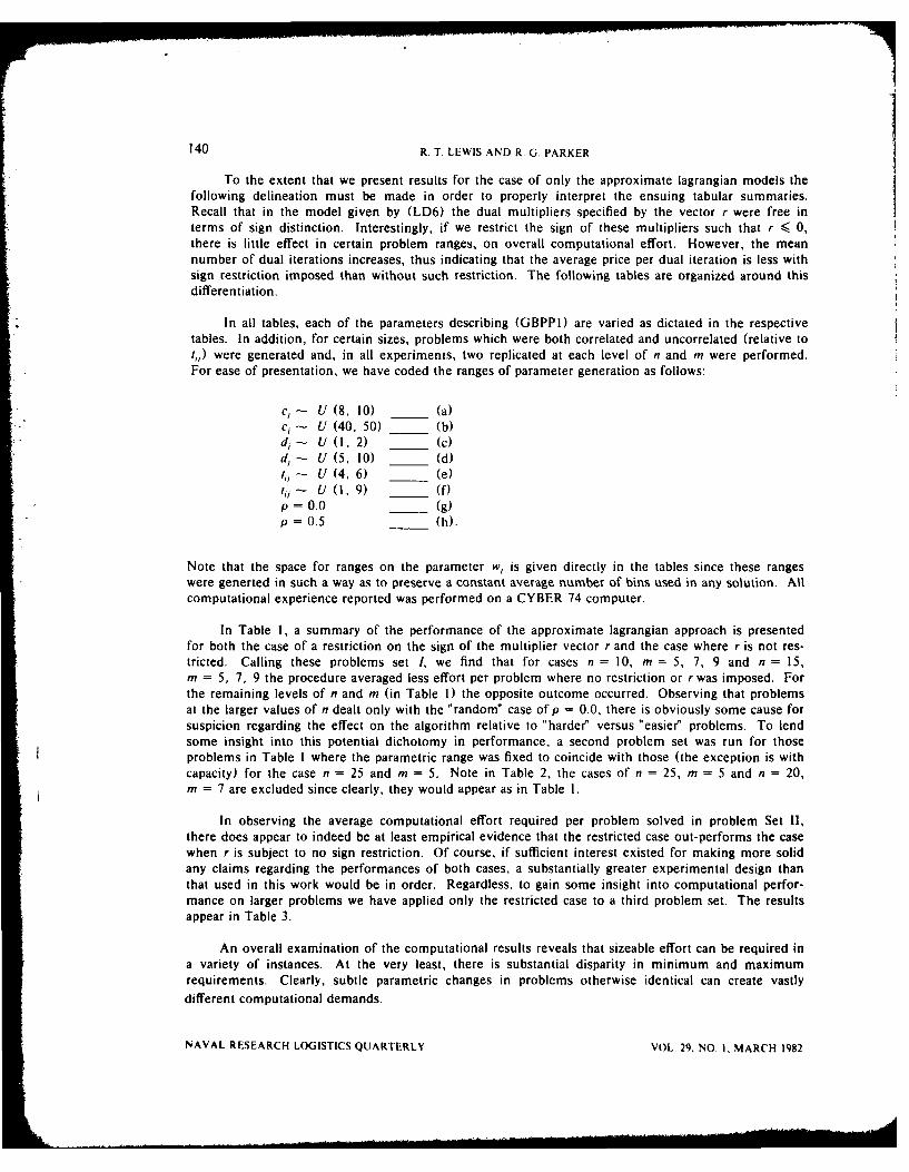
140 R. T. LEWIS AND R. G. PARKER
To the extent that we present results for the case of only the approximate lagrangian models thefollowing delineation must be made in order to properly interpret the ensuing tabular summaries.Recall that in the model given by (LD6) the dual multipliers specified by the vector r were free interms of sign distinction. Interestingly, if we restrict the sign of these multipliers such that r < 0,there is little effect in certain problem ranges, on overall computational effort. However, the meannumber of dual iterations increases, thus indicating that the average price per dual iteration is less withsign restriction imposed than without such restriction. The following tables are organized around thisdifferentiation.
In all tables, each of the parameters describing (GBPPI) are varied as dictated in the respectivetables. In addition, for certain sizes, problems which were both correlated and uncorrelated (relative tot,) were generated and, in all experiments, two replicated at each level of n and m were performed.For ease of presentation, we have coded the ranges of parameter generation as follows:
c,- U (8. 10) __ (a)c, - U (40. 50) __ (b)d, - U (. 2) __ (c)d,- U (5. 10) __ (d)t, U (4. 6) __ (e)t,j U (1, 9) __ (f)p =0.0 __ (g)p = 0.5 (h).
Note that the space for ranges on the parameter w, is given directly in the tables since these rangeswere generted in such a way as to preserve a constant average number of bins used in any solution. Allcomputational experience reported was performed on a CYBER 74 computer.
In Table I, a summary of the performance of the approximate lagrangian approach is presentedfor both the case of a restriction on the sign of the multiplier vector r and the case where r is not res-tricted. Calling these problems set 1, we find that for cases n = 10, m = 5, 7, 9 and n = 15,m = 5, 7, 9 the procedure averaged less effort per problem where no restriction or r was imposed. Forthe remaining levels of n and m (in Table 1) the opposite outcome occurred. Observing that problemsat the larger values of n dealt only with the "random" case of p = 0.0, there is obviously some cause forsuspicion regarding the effect on the algorithm relative to "harder" versus "easier" problems. To lendsome insight into this potential dichotomy in performance, a second problem set was run for thoseproblems in Table 1 where the parametric range was fixed to coincide with those (the exception is withcapacity) for the case n = 25 and m = 5. Note in Table 2, the cases of n = 25, m = 5 and n = 20,m = 7 are excluded since clearly, they would appear as in Table I.
In observing the average computational effort required per problem solved in problem Set 11,there does appear to indeed be at least empirical evidence that the restricted case out-performs the casewhen r is subject to no sign restriction. Of course, if sufficient interest existed for making more solidany claims regarding the performances of both cases, a substantially greater experimental design thanthat used in this work would be in order. Regardless, to gain some insight into computational perfor-mance on larger problems we have applied only the restricted case to a third problem set. The resultsappear in Table 3.
An overall examination of the computational results reveals that sizeable effort can be required ina variety of instances. At the very least, there is substantial disparity in minimum and maximumrequirements. Clearly, subtle parametric changes in problems otherwise identical can create vastlydifferent computational demands.
NAVAL RESEARCH LOGISTICS QUARTERLY VOL. 29. NO. 1, MARCH 1982
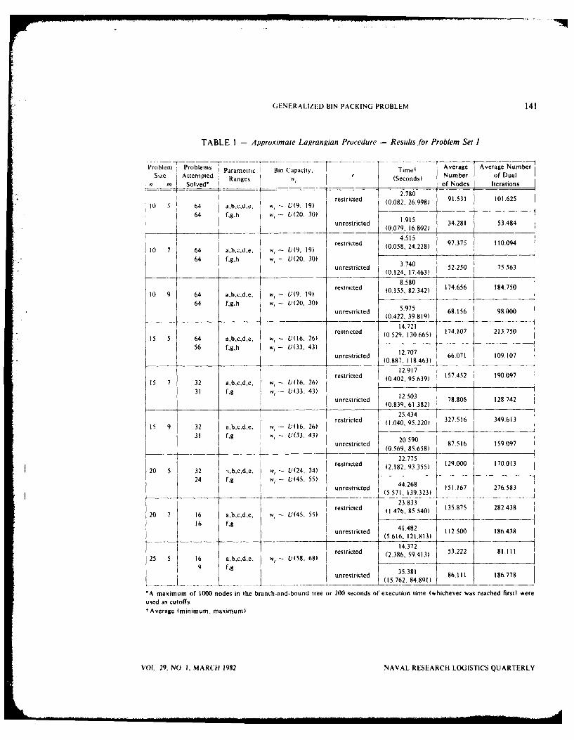
GENERALIZED BIN PACKING PROBLEM 141
TABLE I - Approximate Lagrangian Procedure - Results. br Problem Set I
-role --- Aver-Average NumberProblem Problems I Parametric Bin Capacity, Timet Average
Size Attempted rRanges (Seconds) Number of Dual
n m 4 Solved" I of Nodes Iterations
____ ______-- T1780restricted 2.8) 91.531 101.625
10 5 64 abcd.c. w,- U(9. 19) , 264 f,g,h - U(20. 30) 1.915 34.281 53.484
unrestricted 11 421 5.8(0.0791 16.802)
4.515
10 7 64 a~bcde. w, - (9, 19) restricted (0,058, 24.228) 97.375 110.0941064 a,b,h~~e -i U(2, 3)
64 f,g,hunrestricted w 23 740 52.250 75.563_._unrestricte ~ (0.124, 17.463)
8.580
10 9 64 a~bcde. W] - U (9 19) restricted (0.155, 82.342) 174.656 184.7501064 a~,h~de .,- U(9. 3)
64 fg,h wc - U(20. 30) 5.975 68.156 98000unrestricted_ (0.422, 39.819)
14.721restricted (0.529. 130.665) 174.107 213.750
15 5 64 a,b,c,d,e, w, U16. 26) r
56 f~g,h W)- U(33. 43) unrestricted 12.707 6 109107
(0.887, 118463) 66.07112.917 1 --- 0lrestricted (0.402. 95.639) 157.452 190.097
15 7 32 ab,c,d,e, W, - (16. 26) r ( 9
31 fg w, - U33. 43) unrestricted 12.503 78.806 128.742
(0.839. 61.382)
25 .434restricted (1.040, 95.220) 327.51b 349.61315 9 32 a~b~c~d~e. , v- U(16. 26)
31 f g 0 3 43 u t 20.590 87.516 159.097unrestricted (0.569, 85.658)
22. 77 S
restricted (22.7 3.355) 129.000 170.01320 5 32 .bcde. w, - U(24, 34) ( 9
24 f'g w,- ( 45. 55) 44.268 I 276.583unrestricted (5.571, 276,583restricte (5.476, 859.540) _3_.7
23.833) restricted (1.476, 85540) 135.875 282.43820 7 16 a,b~c,d,e,
1 ( U(45. 55) __
16unrestricted 41.482 112.500 186.438
__unrestricted1(5.616, 121.813) ___14.372
restricted (2.386, 59.413) 53.222 81.11125 5 16 a.b,c,d,e, w, 0 U(58. 68)
9 .. . unrestricted 35.381 86.111 186.778_____----.__________-_____ -____(15.762, 84.891) - ___ _________
*A maximum of 1000 nodes in the branch-and-bound tree or 200 seconds of execution time (whichever was reached first) wereused as cutoffs.t Average (minimum, maximum)
VOL. 29. NO I, MARCH 1982 NAVAL RESEARCH LOGISTICS QUARTERLY
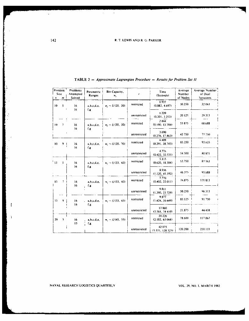
142 R. T. LEWIS AND R. G. PARKER
TABLE 2 - Approximate Lagrangian Procedure - Results for Problem Set I1
Problem Problems Parametric Bin Capacity, Time Average Average NumbeSize Attempted Ranges , r (Seconds) i Number of Dualn m SolvedI of Nodes Iterations
0.937 3 5210 5 16 a,b,c,d,e, w, U(20, 30) restricted (0.082, 4.697) 30.250 32.063
16 f,g 9 1 . . . ......1.209
unrestricted (0.201, 3.253) 20 125 29 313; -- i-2.844 -1I
10 7 16 ab,c,de, w - U(20. 30) restricted (0.190, 13.784) 55.875I 68 688
16 fg 3.690 -
unrestricted (0.276, 17.463) 42.750 77.7504.409
10 9 16 a,b,c,d,e, wi - U(20, 30) restricted (0.291, 38.743) 85.250 93.625S16 f~g ______-
unrestricted 4.776 54500 80.875- unrestricted (0.422, 32.535)
5.11515 5 16 ab,c,d,e, w, - U(33. 43) restricted (0.620, 18.384) 53.750 87 563
16 f'g -8.936 4 9
unrestricted (I.120 45.392) 46.7 95.688 1
1 7.770 1 81 315 7 16 ab,cd,e, w - U(33. 43) restricted (0.402, 22.011) 76.875 12)813
16 f'g9.811
unrestricted (1.390, 23.729) 50.250 96.313
9.877 -
115 9 16 ab,cd,e. w, - U(33. 43) restricted (1.424, 31.649) 83.125 91 75016 fg 13-860 - --
13.860 2 1.44875
unrestricted (3.561, 74.410) 21.875 44.438
20.226 1 1020 5 16 a,bc,d,e, w, U(45. 55) restricted (2.182, 63068) 78.600 117.067
15 fg 42... - .--- -42 .075
unrestricted (5.571, 138.323) 120200 210.133
NAVAL RESEARCH LOGISTICS QUARTERLY VOL. 29, NO. I, MARCH 1982
GENERALIZED BIN PACKING PROBLEM 143
TABLE 3 - Approximate Lagrangian Procedure-Results fbr Problem Set Ill (r restricted only)------- ---------- ---- ---------------- ----- ------
Problem Problems--- -in .. N Ascrdge NumberSize A Parametric Imin eapacitv, T Average Nober 1
SengeAttempted R I H - (Seconds) , Nodes oi DualI n m Solved I I of* o des I- Iterations20 ...9 -
.. . .... : ...- :s: .. 2589 0 97 93820 9 16 a.b,c.d.e, IK, U(4.s.-) 26568 900 0 9[ i 16 f~g |I (3 402. 90 836) 1
16~~~----- ----- ------ -- --- -------290 36i5 7 ~ ~ e 16- ti(58 68) 47984 131 167 207 750
12 -(3 546, 148 0751 -
25 9 1 8 1 a. b,c.d.f. , U(58. 68) 15493 I 115750 125250i I 8 I , (6 420. 27 098) -
~ ~ ------------- --------------- - (64 --- 9830) S 8 i a.b.c.d.f. I v, U(70. 801 23617 202 750 271.875
I 8 g (14446.45554)30) 7-- 8 a abcdf. i, U(70. 80) 37 407 374 250 480.250
8 g (10793.91077)35 5- 8 ab cdf , I U (83,.93) 53194 374 750 656.375i 8 g (10 667, 100,373) ,
405 - ---- a. b. cd.f. WU95, 105)~ 49,607 148.000 1805006 (31.770, 63.353)
45 5 I 4 a.bd.f.g w,- U(120. 130) 92.894 I 364 500 426.250
L 4 (66.278. 125692)
Naturally, the performance of the procedure(s) tested here would be enhanced by direct compari-sons with alternative approaches. The difficulty, however, is that such experience does not appear to beavailable relative to (GPBBI). Of course, various special cases have been examined as suggested earlierand to this extent the procedures tested here may be applied. This sort of comparative analysis wouldsuffer, of course, since the attack presented here would carry unnecessary computational burdens notrequired in treating such special cases. In short, the models we have developed most fully and whichhave been tested in this analysis cater to the full interpretation of (GPBBI). Resolution of specialcases, including the classic bin-packing problem, can be accomplished more efficiently by alternativemeans.
5. SUMMARY
Our entire concentration in this paper has dealt with the optimization of a combinational problemwe have referred to as generalized bin-packing. Of course, one does not require the experience of thistreatise to realize the difficulty of the problem; however, the empirical evidence gathered in thisresearch does indeed tend to dismiss any suspicions to the contrary. In this light, a logical avenuewould likely be to pursue some nonexact approaches to the problem in much the same way as has beendone for the classic bin-packing model.
Of the various heuristic attacks we have postulated and examined, most were constructed directlyfrom optimization procedures, Stated alternatively, specific heuristics involved suitable relaxation ofthe optimization models presented here. In other cases, nonexact schemes were developed as directextensions of the any-fit heuristics discussed in Section 1. In general, procedures of the first categorywere not (empirically speaking) particularly noteworthy in that computational effort frequently rivaledthat of the optimization attacks used. In the latter case, the more ad hoc procedures often generatedsolutions of almost arbitrarily poor quality resulting largely from an inability to make allowances for theunused capacity penalty.
It is worth adding that all testing of heuristic developments has been empirical in that no worst-case analysis was pursued. That this was the case is based not on a lack of interest per se but rather onthe view that such results may be void of the sort of insight presented by similar results for the classicbin-packing problem. Again, the issues here would appear to relate to the arbitrary cost parameterstructure of the problem.
VOL. 29. NO. I, MARCH 1982 NAVAL RESEARCH LOGISTICS QUARTERLY

144 R. T. LEWIS AND R. G. PARKER
REFERENCES
[1] Baker, K., Introduction to Sequencing and Scheduling, (John Wiley and Sons, New York, 1974).[2] Balas, E., "An Additive Algorithm for Solving Linear Programs with Zero-One Variables," Opera-
tions Research, 13, 517-546 (1965).[31 Coffman, E., Editor, Computer and Job-Shop Scheduling Theory, (John Wiley and Sons, New York,
1976).[41 Coffman, E., M. Garey, and D. Johnson, "An Application of Bin Packing to Multi-Processor
Scheduling," SIAM Journal of Computing, 7, 1-17 (1978).[51 De Maio, A. and C. Roveda, "An All Zero-One Algorithm for a Certain Class of Transportation
Problems," Operations Research, 19, 1406-1418 (1971).[61 Eilon, S. and N. Christofides, "The Loading Problem," Management Science, 17, 259-268 (1971).[71 Eilon, S., C. Watson-Gandy, and N. Christofides, Distribution Management (Hafner Publishing Co.,
New York, 1971).[81 Fisher, M., W. Northup, and J. Shapiro, "Using Duality to Solve Discrete Optimization Problems:
Theory and Computational Experience," Mathematical Programming Study 3 (North HollandPublishing Co., Amsterdam, 56-94, 1975).
[91 Fisk, J. and M. Hung, "A Heuristic Routine for Solving Large Loading Problems," Naval ResearchLogistics Quarterly, 26, 643-650 (1979).
[10] Garey, M., R. Graham, and J. Uliman, "Worst-Case Analysis of Some Memory Allocation Algo-rithms," Proceedings of the Fourth Annual ACM Symposium on the Theory of Computing,143-150, 1972.
[I1 1 Garey, M., R. Graham, and J. Ullman, "An Analysis of Some Packing Algorithms," CombinatorialAlgorithms (Academic Press, New York, 39-48, 1973).
[121 Garey, M. and D. Johnson, Computers and Intractability: A Guide to the Theory of NP-Completeness(W. H. Freeman and Co., San Francisco, 1979).
[13] Geoffrion, A. M., "Lagrangian Relaxation for Integer Programming," Mathematical ProgrammingStudy 2 (North Holland Publishing Co., Amsterdam, 82-114, 1974).
[141 Gilmore, P. and R. Gomory, "A Linear Programming Approach to the Cutting Stock Problem: PartI," Opertions Research, 9, 849-859 (1961).
[151 Gilmore, P. and R. Gomory, "A Linear Programming Approach to the Cutting Stock Problem: PartII," Operations Research, 11, 863-888 (1963).
[161 Hung, M. and J. Brown, "An Algorithm for a Class of Loading Problems," Naval Research Logis-tics Quarterly, 25, 289-297 (1978).
[171 Hung, M. and J. Fisk, "An Algorithm for 0-1 Multiple Knapsack Problems," Naval ResearchLogistics Quarterly, 25, 571-579 (1978).
[181 Ingargiola, G. and J. Korsh, "An Algorithm for the Solution of 0-1 Loading Problems," OperationsResearch, 23, 1110-1119 (1975).
[191 Johnson, D., "Near Optimal Bin Packing Algorithms," Doctoral Thesis, Massachusetts Institute ofTechnology, Cambridge (1973).
[201 Johnson, D., "Fast Algorithms for Bin Packing," Journal of Computer and Systems Science, 8,272-314 (1974).
[211 Johnson, D., A. Demers, J. Ullman, M. Garey, and R. Graham, "Worst-Case Performance Boundsfor Simple One-Dimensional Packing Algorithms," SIAM Journal of Computing, 3, 297-325(1974).
[221 Lewis, R.T., "A Generalized Bin-Packing Problem," Doctoral Thesis, Georgia Institute of Technol-ogy, Atlanta (1980).
[23] Padberg, M., "On the Facial Structure of Set Packing Polyhedra," Mathematical Programming, 5.199-215 (1973).
[241 Ross, C. and R. Soland, "A Branch-and Bound-Algorithm for the Generalized Assignment Prob-lem," Mathematical Programming, 8, 91-103 (1975).
[251 Ross, G. and A. Zoltners, "Weighted Assignment Models and Their Application," ManagementScience, 25, 683-696 (1979).
NAVAL RESEARCH LOGISTICS QUARTERLY VOL. 29, NO. I, MARCH 1982
GENERALIZED BIN PACKING PROBLEM 145
1261 Shapiro, J., "A Survey of Lagrangian Techniques for Discrete Optimization," Annals of DiscreteMathematics, 5, 113-138 (1979).
1271 Srinivasan, V. and G. Thompson, "An Algorithm for Assigning Uses to Sources in a Special Class
of Transportation Problems," Operations Research, 21, 284-295 (1973).
VOL. 29, NO. 1, MARCH 1982 NAVAL RESEARCH LOGISTICS QUARTERLY
AN INTEGER PROGRAMMING ALGORITHM FOR PORTFOLIOSELECTION WITH FIXED CHARGES
Mary W. Cooper and Keyvan Farhangian
Department of Operations Researchand Engineering ManagementSouthern Methodist University
Dallas. Texas
ABSTRACT
A mean-variance portfolio selection model with limited diversification isformulated in which transaction and management costs are incorporated as thesum of a linear cost and a fixed cost. The problem is a fixed charge integerprogramming problem solved by hypersurface search using dynamic program-ming. Fathoming is performed in the forward pass of dynamic programming sothat values of the state variable which correspond to infeasible solutions are el-iminated from the tables. This logic permits the solution of problems with 20-30 possible investments.
INTRODUCTION
This paper presents a portfolio selection model for the small investor. A basic reference for theportfolio selection problem is the book of Markowitz [4]. He presents the portfolio selection problemin which there are two criteria for the best portfolio: maximum return and minimum variance. Port-folios are called efficient if they meet either of the following conditions: if for a fixed variance thereturn is maximized, or if the return is fixed and the variance is a minimum. Sharpe [71 subsequentlyintroduced some simplified models in which returns on securities are functions of the performance ofone or more market indices. Recently Pang [6] has formulated and solved the portfolio analysis prob-lem for large scale continuous variable problems by using a modified version of the parametric principlepivoting algorithm for the class of multiple index portfolio problems with positive covariance matrices.In the present paper we follow a different line of research. It has been shown by Jacob [3] that thesolution of portfolio analysis problems by standard techniques generates answers which are inappropri-ate for the small investor because of the large number of positive amounts of different investmentswhich they contain. The individual investor might prefer to limit the total number of his investments sothat he does not have to pay extra charges on odd-lot sales and keep track of the performance of a greatnumber of different securities. Jacob formulated several single index models of the portfolio analysisproblem in which the total number of different investments is contrained. This results in an integerprogramming problem. Faaland solved another integer limited-diversification model parametrically togenerate the set of efficient portfolios [2]. Our work extends his model by allowing transaction andmanagement costs to be expressed explicitly as the sum of linear and fixed charges in the objectivefunction. Then we use a technique for nonlinear integer programming which is based on dynamic pro-gramming [1].
Notation for the Limited Diversification Model
Let us follow the notation for Sharpe's single index portfolio model. The return for security., isRj and
VOL. 29, NO. 1, MARCH 1982 147 NAVAL RESEARCH LOGISTICS QUARTERtLY
148 M. W. COOPER AND K. FARHANGIAN
R,= E,+18,1/ (I) +
where Ej is expected return on security j, I is the current value of the index and E(I) is its expectedvalue, 13j is a parameter and Ej is a random error term with mean zero which is independent of I.Define o' 2(I) and o'2(E) as the variances of those variables and assume that cov(E,, E)) is zero if i ;± j.Following Faaland, the integer problem in which the maximum variance B, is a parametric quantity is
(.1) maximize £ C j
2~ nI:-
(1.2) subject to ( ajXj + y QJXJ2 < B,
j-1 j-1
(1.3) X kJ-I
(1.4) At most Tof the xj may be positive
(1.5) x > 0 j = 1. n
(1.6) x) integer j = 1. n
Let us define Cj = El/k, j = 1. n
a, = f8j o(I)/k, j = 1 ... n.
Q = o,2 (e)/k2, j = 1. n
B, r , t 1 2 ... p.
The new problem includes a commission charge with a fixed minimum plus a component which islinear in the investment amount. Then (1.1) becomes
n(1.7) maximize 7 (C' - V)x, - Ms (x')
j-I
where V is the linear charge, Mj is the fixed charge, and8 X-I1 if Xj > 0
1 (x)1 0 ifxj =O0.
THE INTEGER ALGORITHM
The problem described above (1.2)-(1.7) has several difficult aspects. In (1.2) the representationof portfolio variance is a nonseparable function. One method which can handle such functions is anonlinear integer programming technique called hyperplane search by dynamic programming. Let usoutline this approach. The general method is to solve a sequence of problems of the following formwhich differ only in the value of the right hand side by dynamic programming.
maximize z = f, (x,)
I f3 (x,) - Zk
0 < IK Xu, j= . n
x, integer j = 1. n.
NAVAL RESEARCH LOGISTICS QUARTERLY VOL. 29. NO, I, MARCH 1982
INTEGER PROGRAMMING ALGORITHM FOR PORTFOLIO SELECTION WITH FIXED CHARGES 149
This problem can be used to identify all integer points on any hypersurface level z. If :, is an upperbound on the objective function value, then the solution of the single dynamic programming problemabove can be used to generate all integer points upon the hypersurface level 7.J, = -k and for all righthand side values less than zk. In fact it gives information as to which values of z contain integer pointsso that hypersurfaces with no such points need never be considered, see [1]. We can use this tech-nique on (1.7). Then the constraints of the original problem (1.2)(1.6) are used to test the feasibilityof any candidate integer points, so that the intractability of (1.2) can be overcome. If we choose thesequence (zkl in decreasing order (or generate integer points on hypersurface levels with decreasingobjective function values) then the first feasible point is optimal. If {Zk} is decreasing then this methodis a partial enumeration since no integer points are considered which have objective function values lessthan the optimal solution. This strategy is a direct application of the hyperplane search method to lim-ited diversification portfolio analysis. The complicated form of the objective function (1.7) presents nodifficulty.
A Second Approach
Since the straightforward method given above requires too much storage, the usual method of cal-culating the dynamic programming recursion tables ("pulling') was changed to a second approach whichuses a technique called "pruning" or "fathoming" to reduce the size of the tables by allowing infeasiblepoints to be eliminated during the forward pass. In this way, the constraints (1.2)-(1.4) can be used toreduce computation and storage. The idea assumes that coefficients in the constraints are positive.Under this assumption, if we have a partial solution for which the portfolio variance constraint (1.2) (or(1.3) or (1.4)) is exceeded, then we "prune" the entry or value of element x, which caused the infeasi-bility since no completion of that partial solution will be feasible [5]. This method of fathomingreduces both the storage and computational burden of the algorithm. It supplants the method of check-ing partial solutions for infeasibility at every stage in the backward pass of dynamic programming.
Implementation of the Parametric Right-Hand-Side Feature
The problem (1.2)-(1.7) has a parametric right hand side so that efficient portfolios are generatedfor various upper bounds on portfolio variance. Previous work (11 has shown that such parametricproblems can be solved from a single dynamic programming problem using hypersurface search,because of a similar property obtained in any dynamic programming solution. If an allocation problemis solved for a given right-hand side value, then by completing the last return function table for allvalues of the state variable all problems of identical form but with smaller right hand side values can beobtained.
Computational Results
The model selected for computational results is that given in (1.2)-(1.7), a nonlinear, nonsepar-able parametric fixed charge problem. Problem coefficients were generated randomly for variousnumbers of total possible investments from 10-30. The times for computer runs on the CYBER 73 aregiven in the following table of summary statistics. For each problem size, statistics are averaged for tenproblems with random coefficients. The second through the tenth problems are parametric versions ofthe first and therefore take less time.
This problem is highly specialized. Therefore it is difficult to find computational comparisons withit in the literature. However some recent work on a linear integer bicriteria problem (81 may berelevant. Villarreal and Karwan have given results for three ten-variable problems with four constraintswhich are solved in an average of 18.43 CPU seconds each on a CDC 6400 computer system. Theiralgorithm generates all distinct efficient points (an average of 7) in comparison to ours which generatesefficient points according to ten desired levels of portfolio variance. These authors obtain additional
VOL. 29. NO. I, MARCH 1982 NAVAL RESEARCH LOGISTICS QUARTERLY
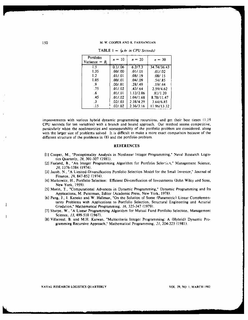
150 M. W. COOPER AND K. FARHANGIAN
TABLE 1 -( ,ak in CPU Seconds)
Portfolio n 10 n = 20 n 30Variance= B
1.5 0.1/.06 6.2/7.3 34.74/36.431.35 .00/.00 .01/.01 .01/.021.2 .01/.01 .08/.19 .08/ 151.05 .00/.01 .04/.09 .54/.85.9 .00/.01 .28/.49 .19/.44.75 .01/.02 .43/.64 2.59/4.62.6 .01/.01 1.12/2.06 .81/1.20.45 .01/.02 1.04/1.68 8.78/11.47.3 .02/.03 2.38/4.29 3.64/6.85.15 .02/.02 2.36/3.16 11.96/13.32
improvements with various hybrid dynamic programming recursions, and get their best times (1.19CPU seconds for ten variables) with a branch and bound approach. Our method seems competitive,particularly when the nonlinearities and nonseparability of the portfolio problem are considered, alongwith the larger size of problems solved. It is difficult to make a more exact comparison because of thedifferent structure of the problems in (8) and the portfolio problem.
REFERENCES
[11 Cooper, M., "Postoptimality Analysis in Nonlinear Integer Programming," Naval Research Logis-tics Quarterly, 28, 301-307 (1981).
[2] Faaland, B., "An Integer Programming Algorithm for Portfolio Selectict,," Management Science,20, 1376-1384 (1974).
[31 Jacob, N., "A Limited-Diversification Portfolio Selection Model for the Small Investor," Journal ofFinance, 29, 847-852 (1974).
[4] Markowitz, H., Portfolio Selection: Efficient Diversification of Investments (John Wiley and Sons,New York, 1959).
15] Morin, T., "Computational Advances in Dynamic Programming," Dynamic Programming and ItsApplications, M. Puterman, Editor (Academic Press, New York, 1978).
[6] Pang, J., I. Kaneko and W. Hallman, "On the Solution of Some (Parametric) Linear Complemen-tarity Problems with Applications to Portfolio Selection, Structural Engineering and ActurialGradation," Mathematical Programming, 16, 325-347 (1979).
[7] Sharpe, W., "A Linear Programming Algorithm for Mutual Fund Portfolio Selection, ManagementScience, 13, 499-510 (1967).
181 Villarreal, B. and M.H. Karwan, "Multicriteria Integer Programming: A (Hybrid) Dynamic Pro-gramming Recursive Approach," Mathematical Programming, 21, 204-223 (1981).
NAVAL RESEARCH LOGISTICS QUARTERLY VOL. 29, NO. I, MARCH 1982
SCHEDULING OF A SINGLE MACHINE TO MINIMIZETOTAL WEIGHTED COMPLETION TIME SUBJECT TO
RELEASE DATES
Lucio Bianco and Salvatore Ricciardelli
Jstituto di Analisi dei Sistemi ed Informatica del CNRRome, Italy
ABSTRACT
In this paper the nIl/r, > O/F, wC, problem under the assumptions ofJ
nonpreemptive sequencing and sequence independent processing times is inves-tigated. After pointing out the fundamental properties, some dominancesufficient conditions among sequences are obtained and a branch and bound al-gorithm is proposed. Computational results are reported and discussed.
1. INTRODUCTION
The one machine scheduling problem has been studied extensively under different hypotheses andobjective functions. Nevertheless, in the literature, emphasis is laid upon the case with equal readytimes, no imposed due dates and flow time (or equivalent function) as objective function. In this con-text the problem solution is trivial since the Smith's rules [141, well-known as shortest processing time(SPT) rule and weighted shortest processing time (WSPT) rule, provide an optimal solution. Accord-ing to these rules, jobs are sequenced on the basis of a preestablished order of their processing times.
In [7], [8], 1121, 1131, and [15], a more sophisticated cost function, such as weighted tardiness, isadopted for it turns out to be a suitable model for many real problems in which jobs may be consideredavailable simultaneously for processing on a single machine in order to minimize the total sum of thedelays with respect to their due dates. One of the most constraining assumptions is equality of theready times of the jobs.
As a matter of fact, whenever different ready times are to be considered (r, > 0). the previousmodels and the corresponding algorithms are no more adequate.
The case r, > 0 has been recognized in research on other single machine problems, where duedates were also taken into consideration [11, [51, and [101. However, in these works, the authors inves-tigate the properties of a rather different cost function given by the maximum lateness (or tardiness)with weights w, = I for all j.
In [21, [31, (4], and [II], refer-ing to scheduling theory application to air traffic control, minimiz-ing total weighted waiting time in one machine scheduling problem with unequal ready times has beenconsidered.
An implicit enumeration procedure has been developed and a simplified algorithm (w, - I,-Vj)has been implemented in order to work in real time. The interested reader may address to referencesI111 and 141 for a complete discussion of this ,,pplication. The aforementioned scheduling problem,although simple in these terms, is not trivial and it may be proved to be NP-complete [9]. The maindifficulty arises from the fact that, since r, _> 0, idle times may be inserted in the optimal schedule [61.
VOL. 29. NO I, MARCH 1982 151 NAVAL RESEARCH LOGISTICS QUARTERLY
152 L. BIANCO AND S. RICCIARDELLI
In this paper, starting from the results obtained in previous works of ours [2], [3], (4], and [11]the n/l/r, > 0/ 7- wC problem, with no preemption allowed and sequence independent processing
times, is analyzed. The purpose is to establish some further dominance properties and above all topresent a much improved branch and bound algorithm. Computational results, obtained with this algo-rithm, are also reported and discussed.
2. DEFINITIONS AND PROBLEM STATEMENT
Let N = {jlj = 1.2 ..... n} be a set of jobs to be processed, one job at a time, on a single, con-tinuously available, machine. For each job j, the ready time r,, the processing time p,, and the weightw,, are given.
We call sequence on set K c N any permutation in K which is indicated with sk, being so thesequence on the void set. Completion of all jobs requires establishing a sequences, = (J11 .J1 21 . i. When a job parameter is identified by the job's position in a given sequencerather than its index number, the position is indicated in square brackets. Thus C[,1 means the comple-tion time of whichever job occupies the ]th position in the sequence.
Suppose now that a sequence is constructed by adding one job at a time, starting from position 1.At any step, we have a partial sequence Sk = (J[11 J121 ... Jilkl) of a job set K C N. It can easily beverified that, in our setting, the completion time of such a sequence cannot be expressed only in termsof processing times regardless of the order in which jobs are scheduled, since idle times can be inserted[6]. This fact suggests some useful definitions.
DEFINITION 1: Given a partial sequence sk., the earliest start time of a job j E K, where
K = N - K is the set of jobs not sequenced, can be expressed as
(1) t,(sk) - max (r i , CIk)
with t,= r1 . 'j E N, if k 0.
DEFINITION 2: Given a partial sequence Sk, the completion time of a job j E K. C,(sk), can be
expressed as
(2) C,(sk) = t,(Sk) + pi.
DEFINITION 3: Let K be any subset of N with cardinality k, then the cost function associated to sk isk
C'(sk) s uldcw
If k = n, C(s,) expresses the total weighted completion time of s,.
Then, the problem can be formally stated as follows: Given a job set N, find a sequence s,* such that
C'(s*) < (W(). Vsn E SN.
To fully understand the problem framework, it is suitable to introduce the reduced problem con-cept. A definition of reduced problem may be found in references [71 and 115]. However, thatdefinition is given by considering the sequence completion time as computed regardless of the order ofthe jobs. As pointed out before, this is impossible in our setting- a more general definition, which alsoholds in our hypotheses, is the following.
NAVAL RESEARCH LOGISTICS QUARTERLY VOL. 29, NO. 1, MARCH 1982
SCHEDULING SINGLE MACHINE TO MINIMIZE TOTAL COMPLETION TIME 153
DEFINITION 4: A problem is said t6 be reducible if a partition (NI, N 2) of set N exists suchthat, if s*, s*, s' are the optimal sequences with respect to C'(') on N. N1,. N2, respectively, it is truethat s, = s* s2.
REMARK 1: It is easy to prove that a given problem n/l/r, > 0/. wjC is certainly reducible if
job set N, and a corresponding optimal sequence s, exist such that completion time of s) is less than(or at most equal to) the earliest ready time associated with N 2.
In [11] a simple decomposition method to transform a given problem into reduced problems is
outlined.
Therefore, without loss of generality, from now on, only reduced problems will be dealt with.
DEFINITION 5: Given a partial sequence sk, a job set V C K is said to be "dense" if anysequence Jl, J2. J, on Vhas no inserted idle times.
It is easy to verify that
j E V iff I(sk) < min Csk).)EK
DEFINITION 6: Given two sequences Sk and Sh both belonging to set S, sk dominates sh, if andonly if, it is true that there exists an Sn-k such that Sk Snk = s' belongs to SN and
C'(s') < Cw(slI sh) for all snIsh.
DEFINITION 7: Two sequences, sk and sh, are equivalent
if C4(s*Isk) = C'(SnISh).
REMARK 2: On the basis of the previous definitions it follows immediately that an optimalsequence s* dominates any other one, and it is equivalent to all its own partial sequences sk,k - l.2 .... n.
DEFINITION 8: A sequence is said to be an ECT sequence if it satisfies the earliest completiontime (ECT) rule, i.e., if CIk+lI = min C(sk), 0 <, k < n - I.
jEK
Ties are broken by choosing j with min t, and further ties by choosing J with max w, and, at last,by choosing j with min j.
DEFINITION 9: A sequence is said to be an EST sequence if it satisfies the earliest start time(EST) rule, i.e., if each actual job start time is such as
T[, I I= min t,(sk), 0 < k < n- 1.AEK
3. OPTIMALITY AND DOMINANCE CRITERIA
In this section a set of properties, which enhance the efficiency of the search for an optimal solu-tion, is given. Some of these properties (specifically those resulting from Theorems 2, 3, 4, 5 andCorollary 2) have already been demonstrated in a previous paper I Il]. The other properties, expressedas Theorems 1, 6, 7 and Corollaries I and 3, have here been carried out in order to improve the algo-rithm performance. Extended proofs of these further properties are reported in the Appendix.
VOL. 29, NO. 1, MARCH 1982 NAVAL RESEARCH LOGISTICS QUARTERLY

154 L. BIANCO AND S. RICCIARDELLI
THEOREM 1: Given a job set N and a partial sequence sA(k < n). if, for i E T
(a) -L-. Vj E KW, W,
(b) t,(s,) < t,(s,). h E K
then ski"dominates" sAih.
Clearly, the property expressed in Theorem 1, in the case with K,; = I V i, can be applied in thefollowing way: "Given a partial sequence sk, consider, among all the remaining jobs, job i with the leastprocessing time and then take out of consideration for k + I th position, all jobs unable to start beforejob i. This property, of course, appears to be efficient since earlier job i is able to start. For instance, ifjob i has both minimum processing time and earliest start time, no other job may be considered for pos-sible inclusion in the (k + l)th position in the sequence.
COROLLARY 1: An EST sequence of job set N is optimal if it is ordered according to WSPTrule.
THEOREM 2: Given a job set N, a partial sequence sk (k < n) and two jobs ij E K. Ifr, > C 1(s,), then skidominates ski.
From this theorem it follows that is is possible to restrict search for optimal solution to the classof active schedules [Ii.
In Figure 1 an example of the application of Theorem 2 is given.
K- jh,i,l,m)
------ h,i are candidates
Scheduled jobsELZIJ :l,m are not candidates
C (k] min C C.(s k time
FtcLRL I Example of application of Theorem 2i candidates to (A + 11thposition in the sequence+
THEOREM 3: Given Sk and two jobs i. j E K, if
(a) w, >,w
(b)CQk] jE, Cj(Sk)
(c) w,[C(s k) - C,(Sk)] + wip,- w,p, 1 (p,- p) . WIEQ
where Q is the set 2 - i I), then skidominates Ski-
NAVAL RESEARCH LOGISTICS QUARTERLY VOL 29. NO. 1, MARCH 1982
SCHEDULING SINGLE MACHINE TO MINIMIZE TOTAL COMPLETION TIME 155
THEOREM 4: Given sA and two jobs i, j E K, if
(a) w, > w,
(b) C,(sk) < C,(sk)
(c) w,p, - wp, >, [C,(sk) - ('-(Sk)] I w, + 8 _1 (p, - p,)
W I- Wj
then skidominates Sk.
Properties resulting from Theorems 3 and 4 may be practically utilized in order to operate afurther selection within the class of active schedules. Of course, from a theoretical point of view theycould also be applied within the more general class of permutation schedules. It is easily seen that, ingeneral, the dominance concept, as expressed in Theorems 3 and 4, depends not only on the input vari-ables (weight coefficients, processing and ready times) associated to the couple of jobs taken into con-sideration but also on the input variables associated to the remaining jobs (specifically on their weightcoefficients or on their number if K, = I V i ).
THEOREM 5: Given a job set N and two partial sequences xiyj and xjyi. If
(a) iyj and jyi have no inserted idle times
(b) IC,(x) - C,(x)1 .Y ' + w, - wjl P + wipt - wAtEP IAP
W( - t,(X) ,I A WL
where P is the job set of iyj and U the set N - P - (x then xiyj dominates xjyi.
COROLLARY 2: Given s4 and two jobs i, j E K. Let K be the set "dense," if
(a) w, > W,
(b) t,(sA) >1 t,(sk)
(C) Qsk) > C,(sk)
then Ski dominates Ski.
THEOREM 6: Given a job set N and a partial sequence sk(k < n), for any sequence (sl sk) alower bound _"(sflsk) < C'(s.lsk) exists, where
'7-k
_'(s~lSk) = C'(sk) + : Wk4,Ck+,(Sk)i-I
n-A-I n-k+ 1". !. IsICk,(s,) - tk+l(Sk)l
i-I1 I--il
- 8-1 [Ck+,(sk) - CA,,(sA)]) - min(wk+,, wk+,),
being k + jand k + I E Rwith r+ + rk+I.
The first term of the lower bound provided by Theorem 6 is, simply, the value of the objectivefunction associated with the partial sequence Sk. The second term takes into account that each job ofthe complementary set K cannot start before its earliest start time. The third term takes into accountthat processing times of the unscheduled jobs are not to be overlapped in the final sequence.
VOL. 29, NO. I. MARCH 1982 NAVAL RESEARCH LOGISTICS QUARTERLY

156 L. BIANCO AND S. RICCIARDELLI
An example of application of this lower bound is reported in Figure 2.
00hii
C[1) C[2] C [k] Ch c c1 time
W (sn/Sk )=WIll C] + -.... Wk]C k]+ WhCh+ W i-C- C+ W1C1+Ohi. min (WiW h )
+0 hl' min (W I hr O h i+ 1 1 m1n (Wi r Wi
FitLRE 2. Example of lower bound computation for a partial sequence sA,
THEOREM 7: Let s° be a sequence on N such that, for 0 < k < n - I
(a) Tt,+t =Cik1
(b) C[All = min Ci(sk)iSA
(c) wlk I :-, Wlk~ll
being Cl01 = r,, i E N, then s, dominates any other sequence sn' of the same set starting with job hsuch as r, < rh.
COROLLARY 3: An ECT sequence, defined on a job set Nand ordered according to nondecreas-ing weights, is optimal if it has no inserted idle times and begins with the job having the smallest readytime.
4. THE PROPOSED APPROACH
To solve the problem under study, an implicit enumerative procedure is proposed, 'based upon abranch and bound concept. It involves a search along the branches of a tree, in which any node at levelk represents a partial sequence sk defined on a set K with cardinality k.
As a consequence, subsequent jobs in sk correspond also to a succession of nodes encountered bygoing from tree root so to node sk. For each node sk , as illustrated in Section 3, a lower bound
"(s, Jsk) on C'(sJsk) is computed, and the current optimal solution is utilized as upper bound. Ateach iteration, the node being expanded is called the current node, whose last job has the lowestcurrent value of earliest start time. A closed node is one whose correspondent partial sequence hasbeen dominated and, therefore, it will be no longer considered. To identify dominated nodes, someelimination conditions based upon the previous theorems are then applied. In this way, the number ofnodes branching from the current node can be effectively reduced.
NAVAL RESEARCH LOGISTICS QUARTERLY VOL. 29, NO. 1, MARCH 1982

SCHEDULING SINGLE MACHINE TO MINIMIZE TOTAL COMPLETION TIME 157
The proposed procedure is a recursive one. In fact, whenever a partial sequence sk on N has beenfixed, the optimal sequencing problem of the jobs belonging to set K is identical to the initial problemif their ready times are shifted so that none of them is less than C(sk).
5. THE ALGORITHM
The algorithm consists of three basic phases: initialization, branching and termination. Initializa-tion involves defining initial value of the variables, determining an initial sequence and testing it foroptimality.
Branching is an iterative procedure. In each iteration, it generates the descendents of the currentnode, eliminates closed nodes, updates the set of job candidates to successive position, identifies, asnext current node, that one having last job with lowest earliest start time, and computes the lowerbound for it.
The termination phase consists of identification of the optimal sequence s° and computation ofC'(s*).
Initialization
(1) Let Nbe the job set (ilJ - 1,2. n). Define the corresponding parameter sets:
R {ri, r2 ..... r ..... r}, P - {p1, p2 ..... PJ}
W Iw., w2 . ... W,,J where rn_!-. ri <, jr+1.
If r, = r+1 call jjob with min p
(2) k - 0, K - 0, sk = 0, K = N, C(sk) ri.
(3) Construct an initial solution 3, by means of an heuristic rule (for example EST or ECT) andcompute C*(3n).
(4) Test initial solution for optimality by means of Corollary I and Corollary 3. If .,, passes thetest go to Step 22.
Branching
(5) Determine tj(sk) - max Ir,. C(sk)} and
Cm(S k ) - min (ti(sk) + Pi)IEA
(6) Form the set
Dk - (jlj E k, ti(sk) < C-(sk)}
(7) If D, = K go to Step 18
(8) Generate nodes Ski, Vj E D5
(9) For each node ski dominated according to some of the Theorems 1, 3, 4, 5 (and Corollary 2(if Step 8 has been reached coming from Step 19)), update set DS, by setting
D - D - j
VOL. 29. NO. I, MARCH 1982 NAVAL RESEARCH LOGISTICS QUARTERLY
158 L. BIANCO AND S. RICCIARDELLI
(10) Set k = k + I
(1I) IfD,_ = 0, set k = k- I and go to Step 16
(12) Seto,,_ D D f, - s Sk--I, K = (sk}, K N- K with j': t, min t,(ski)IE I),
(13) Compute lower bound C'(s.l1sk)
(14) If C'(s,,IsA) > C'(3,) go to Step 11.
(15) Set C(sA) = t, + pi,and go to Step 5.
(16) lfk =0, go to Step 22.
(17) Go to Step It.
(18) If ti(s k ) = t. Vj E K, go to Step 20.
(19) Go to Step 8.
(20) Form the sequence SkS,_k, where s,-k is the sequence on K satisfying the WSPT rule.
(21) Set 3,, = SkS,-k' C'(3_) = C'(SlI Sk) and go to Step 11).
Termination
(22) Set s, = 3, and C"(sn) = C'(3,,). STOP.
Figure 3 shows a synthetic flow-chart which illustrates the algorithm logic.
6. COMPUTATIONAL RESULTS AND CONCLUSIONS
The algorithm, previously illustrated, has been implemented on a Digital PDP 11/34 minicom-puter.
Different series of tests have been performed by considering a given number of jobs n - 10. Foreach series the p, values have been chosen uniformly distributed over a fixed interval [I + 71 and the r,values have been chosen uniformly distributed over five different time intervals of growing length.Moreover, for each fixed range of r,, the weights have also been taken as uniformly distributed overten different intervals of growing length. The results are fully reported in Table I while in Figures 4and 5 are reported the diagrams showing the number of nodes generated versus max r, and max w,respectively. As it can be observed a significant increase in all the parameters is met whenever weightcoefficients tend to be unequal. In particular, computational results show that changes in the observedparameters are relatively less dependent on the width of the weights range. Rather, these changes seemto arise whenever a mere difference among the weights is considered. Figure 4 and 5 show thisbehavior for the number of nodes generated.
Nevertheless, the computation time, in the worst case, does not exceed a few tens of seconds,even though a fast computer has not been used.
A last remark, involves the fact that the typical behavior (bell-shaped), observed in (41 whenw, = I, V j, is confirmed also if w, are distributed on a fixed interval (Figure 4).
NAVAL RESEARCH LOGISTICS QUARTERLY VOL. 29, NO. 1, MARCH 1982
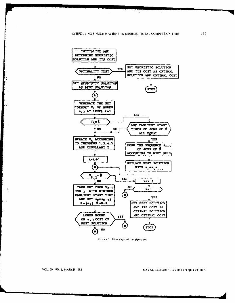
SCHEDULING SINGLE MACHINE TO MINIMIZE TOTAL COMPLETION TIME 159
t [ INITIALIZE AND
SDrEE1INE HEURISTIClSOLUTION AND ITS COST|
(OPTIMALTY TEST AND ITS COST AS OPTIMALI!NO SOLUTION AND OPTIMAL COSTIJ-"SE Hs, EURISTIC SO,-UTIONI
| AS BEST SOLUTION G ..-,
.IM *PAGEEATE THE SETDES-Vk OF NODESi
lkskj AT LEVEL k 1 YE
SNO NO TIM4ES OF JOBS OF K]
TO THEOREMStI ,3,4,5|S_
AND COROLLAY 2 IE SEOQUEoCs oF nI ACCOIMING TO WSPT RULEI
| ~WITH an S-n8!-1
JOB J' WITH KI I k-0ELIEST ST RT TIMEAD S T I - k l
E
K-18k), It -- K S ET BEST SOLUTIONl I AND ITS COST AS
OPTIMAL SOLUTIONLOWE BOUD YE AND OPTIMAL COST
ON 8k lCOST OF\BESTSOLUrIONB
h-(t Itl Flow chart of I li algorithim
VOL. 29, NO. 1, MARCH 1982 NAVAL RESEARCH LOGISTICS QUARTERLY
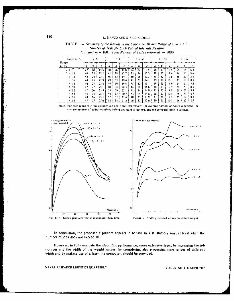
160 L. BIANCO AND S. RICCIARDELLI
TABLE I - Summary of the Results in the Case n = 10 and Range of p, = 1 + 7.Number of Tests for Each Pair of Intervals Relative
to r, and wj = 100. Total Number of Tests Performed 5000Range of r, I + 20 7 -30 I + 40 I 50
Range i 1 - IIT-- i- ' ...-- -- -ofW. a Ib c a b c a b c _ a I b c a I b c I
I 27 18 14.5 30 26 128 24 22 9.5 16 13 7,5 15 5 681.2 44 25 22.2 42 29 17.7 35 24 12.3 28 22 9.6 24 120 861
I 1 4 42 24 22.1 46 32 19. 40 28 13.3 31 22 9.81 25 20 86I 1.6 44 2 22.9 49 33 194 41 j 32 14.1 29 22 10 25 19 88+ 1.8 44 25 23.8 49 30 19.4 45 32 15 29 25 9.9 124 20 . 8.81
1 2.0 47 27 25 48 34 20.3 44 34 14.6 301 23 9.9 26 20 88' 2.2 47 26 25.5 55 39 22 (41 34 14'9 31 25 1 9.8 26 21 8.9,I 2.4 46 127 25.1 48 32 20.2 43 29 14.8 28 23 1I 0.1 26 211 8 7
1 2.6 48 26 25.1 52 37 21.4 40 31 13.9 27 22 9.7 25 19 8811 2.8 47 25 25.6 52 35 21.2 40 32 13.6 30 25 0.1 26 22 8,7
Note: For each range of r, the columns ab and c are, respectively, the average number of nodes generated, theaverage number of nodes examined before optimum is reached, and the computer time in seconds.
Aserage number of Number of nodes generatednodes generated W - 1 2.2 IJ
W -2.650
axmu rM-t 1 2
40 40 14
it) 30 1 S
20) 20
20 30 40 50 60 I 2 3
FIGURE 4. Nodes generated versus maximum ready time FIGURE 5. Nodes generated versus maximum weight
In conclusion, the proposed algorithm appears to behave in a satisfactory way, at least when thenumber of jobs does not exceed 10.
However, to fully evaluate the algorithm performance, more extensive tests, by increasing the jobnumber and the width of the weight ranges, by considering also processing time ranges of differentwidth and by making use of a fast-time computer, should be provided.
NAVAL RESEARCH LOGISTICS QUARTERLY VOL. 29, NO. 1, MARCH 1982

SCHEDULING SINGLE MACHINE TO MINIMIZE TOTAL COMPLETION TIME 161
REFERENCES
[ll Baker, K.P. and Zan-Sing Su, "Sequencing with Due-Dates and Early Start Times to MinimizeMaximum Tardiness," Naval Research Logistics Quarterly, 21, 171-176 (1974).
(21 Bianco, L., B. Nicoletti, and S. Ricciardelli, "An Algorithm for Optimal Sequencing of Aircraft inthe Near Terminal Area," Proceedings of the 8th IFIP Conference on Optimization Techniques(Springer Verlag, Berlin, 1977).
(31 Bianco, L. and S. Ricciardelli, "11 Problema del Sequenziamento Ottimo Degli Aerei in Area Ter-minale," Rapporto dell'lst. di Automatica dell'Universiti di Roma e del C.S.S.C.C.A.-C.N.R. -R. 78-10 (1978).
141 Bianco, L., S. Ricciardelli, A. Sassano, and G. Rinaldi, "The Aircraft Optimal Sequencing as an NJob One Machine Scheduling Problem," EURO 1Il - Amsterdam (1979) and Rapporto dell'lst.di Automatica dell'Univ. di Roma e del C.S.S.C.C.A.-C.N.R., R. 79-36 (1979).
151 Bratley, P., M. Florian, and P. Robillard, "On Sequencing with Earliest Starts and Due-Dates withApplication to Computing Bounds for the (n/m G/F max) Problem," Naval Research LogisticsQuarterly, 20, 57-67 (1973).
(61 Conway, R.W., W.L. Maxwell, and L.W. Miller, "Theory of Scheduling" (Addison-Wesley Publish-ing Co., Reading, MA, 1967).
[71 Emmons, H., "One Machine Sequencing to Minimize Certain Functions of Job Tardiness," Opera-tions Research, 17, 701-715 (1969).
18] Fisher, M.L., "A Dual Algorithm for the One-Machine Scheduling Problem," Mathematical Pro-gramming, II, 229-251 (1976).
[9] Lenstra, J.K., A.H.G. Rinnoy Kan, and P. Brucker, "Complexity of Machine Scheduling Prob-lems," Studies in Integer Programming. (North-Holland, Amsterdam, 1977).
[10] McMahon, G., and M. Florian, "On Scheduling with Ready Times and Due Dates to MinimizeMaximum Lateness," Operations Reserch, 23, 475-482 (1975).
(I 1I Rinaldi, G. and A. Sassano, "On a Job Scheduling Problem with different Ready Times: Some Pro-perties and a NF-w Algorithm to Determine the Optimal Solution," Rapporto dell'Ist. diAutomatica dell'Universita di Roma e del C.S.S.C.C.A.-C.N.R,R., 77-24 (1977).
[12] Rinnoy Kan, A.H.G., B.J. Lageweg, and J.K. Lenstra, "Minimizing Total Costs in One-MachineScheduling," Operations Research, 23, 908-927 (1975).
[13] Shwimer, J., "On the N-Job, One-Machine, Sequence-Independent Scheduling Problem with Tardi-ness Penalties: a Branch-bound Solution," Management Science, 18, B301-B313 (1970).
[14] Smith, W.E., "Various Optimizers for Single-Stage Production," Naval Research Logistics Quar-terly, 3, 59-66 (1956).
[15] Srinivasan, V., "A Hybrid Algorithm for the One-Machine Sequencing Problem to Minimize TotalTardiness," Naval Research Logistics Quarterly, 18, 317-327 (1971).
APPENDIX
Proof of Theorem I:
Consider a schedule S, = SkSn-k having h in position k + I and i in position y > k + 1. Let s'
be a schedule that differs from s, only in that job i is interchanged with its immediate predecessor .i inposition v - I. The first (v - 2) jobs have exactly the same completion times under s. and s, and,therefore make the same contribution to total weighted completion time.
Schedules s, and s, differ only in the completion times of the (n - y + 2) remaining jobs.
As far as the last (n -. y) jobs are concerned, which are the same in both sequences, it can bederived that
(I) AC"(y) = w l w1 jCl(s) - wllCul(S," , 0.
VOL. 29. NO. I, MARCH 1982 NAVAL RESEARCH LOGISTICS QUARTERLY
162 L. BIANCO AND S. RICCIARDELLI
In fact, by assumption b), it follows that
CtL(s,,) - max (C,_ 2 , rj) + p + pi
CL (s',) = max((CL- 2 + p,), rj} + pp
where j is the job in position y - 1. Hence, it is easy to verify thatCtL](s.) > CtL(s,)
from which the (1) immediately follows.
Let's examine now contribution of jobs h and i. If we call t = CL- 2j(s,), then their weightedcompletion times can be expressed by the following:
Under sn:
wCj = wv1_C[Ly-1 = w.tmax(t, rj) + pj)
w =C, = wyjCLl= wimax (t, rj) + p + pJ;
Under s,:
w- Cj = wtLCtj = wj [max (t + p,), r1j + pjl
wCi = wLyjj] CLjj1 = w,(t + pi),
since, by assumptions b), ri < < th < t.
Two cases exist:
(1) ri < t
Eliminating common terms, from the (1) and assumption (a), it follows that
CW(sn) - Cw(s,) = ACW(y) + wpj - w-p, > 0
(2) rj > t.
In this case
Cw(s") - CW(s') = ACW(y) + wj (rj + p,) + w,(ri + pi + pi)
- wj{I[max (t + pi), r1 + pj} - w,(t + p,).
Two subcases are to be considered:(2a) rji > t + p,.
From this and inequality (1) it follows that
Cw(s.) - Cw(s" ) = ACW(y) + w, (rj + p, - t) > 0
(2b) rji < t + pi.
In this subcase, it is easy to verify that
Cw(sn) - Cw(s,) - ACw(y) + (wj + w,) (r, - t) + (wP, - w.,P,) > 0
since the first and third terms of the sum are nonnegative, by (1) and assumption (a), respectively, andthe second term is positive, being rj > t.
NAVAL RESEARCH LOGISTICS QUARTERLY VOL. 29, NO. 1, MARCH 1982
SCHEDULING SINGLE MACHINE TO MINIMIZE TOTAL COMPLETION TIME 163
Hence, in conclusion, s, represents an improvement over s,. One could repeat the interchangeoperation on s, by shifting job i backward into position y - 2 and advancing the corresponding job intoposition y - 1. In this way the new sequence obtained is better than s,.
By induction, it is possible to repeat this operation on s,, until job i reaches position k + 2. Thenit follows that apartial sequence skhi dominates every other partial sequence skhj, where j * h and i isan element of K.
To complete. the proof let's consider now as schedule s, the one with jobs h and i in the (k + I)th
and (k + 2)th positions, respectively.
Therefore s,, differs from s, in that job i is in position k + I and job h in position k + 2.
In this case, since t = Cik](S,) can be < r, only the completion times of s, must be rewritten asfollows:
Under s,:
W =Ch Wlk+2]Ctk+ 21 = wh{max[max(t, r) + P,, rh] + ph)
wC, = Wtk+llCIk+l- wmax(t, r) + pd}.
Three cases exist. Cases (1) and (2) have already been examined. Hence, one needs only toanalyze the following:
(3) 1 <
From assumption (b) and definition of t, it is also true that r < rh. Hence,
Cw(s,) - Cw(s,) = ACw(k + 2) + wh(rh + Ph) + wi(rh + Ph + pi)
- Wh ((max (ri + pd, r I + Ph) - w (ri + Pd.
Two subcases are then to be examined:
(3a) rh > r, +p,.
In this hypothesis it follows immediately that
Cw(sn) - Cw(s, ) = ACw(k + 2) + wi(r h + Ph - r,) > 0
(3b) rh < ri + pi.
It is easy to verify that
CW(sm) - Cw(s,) = ACW(k + 2) + (wh + w,) (rh - r,) + (wPh - WhP) )> 0
since all terms of the sum are nonnegative by (1), assumptions (b) and (a), respectively.
In conclusion s, is better than sn.
Hence, since skhi dominates every sequence with skh fixed and skih always dominates sk hi, it fol-lows that i dominates h in position k + I. Q.E.D.
Proof of Corollary i.
VOL. 29, NO. 1, MARCH 1982 NAVAL RESEARCH LOGISTICS QUARTERLY
164 L. BIANCO AND S. RICCiARDELLI
It follows immediately from the previous theorem.
As far as theorems 2, 3, 4, 5 and Corollary 2 are concerned, they have been proved in [1I]
Proof of Theorem 6:
It can be immediately seen that, for k = n, CW(s_ ) =Cw(sn). Then it is only necessary to prove
that for every k, CW(s, Is) < CW(s, Is+).
CW(snlIsk) and CW(sn lsk+I) can be expressed in the following way:
CW(S, 14s) -C'(Snl1k11) + C"(SISk+l)
CW (S Is k C'(SnI Sk ) + C"(SnlIk)
wheren-k-I
fj'(Sfl~Sk+l) Cw(sk) + Wk+ICk+I(sk) + I Wk+jCk+I+j(Sk+i),
n-k-I n-k j=
f"(SnISk+I) I I 18[Ck~j(sk~l) - tkll(Sk+i)]j-2 1-j+1
-.-. 1 [Ck+j(sk+l) - Ck+,(sk±,I min (wk+,, wk+,);
n-k-I
C'(SnlSk) = C(Sk) + Wk+]Ck+j(sk) + 1: Wk+i+ICk+]+j(Sk)
+ Y, (8.1[Ck+](sk) - tk+I(Sk)] - 8-1 [Ck41 (Sk) - Ck+l(sk)]).1-2
*min (wk+I, wk+,);
C "(Sn ISk) = n-k-i n-k {&.-Itk+,(sk)
j-2 1-j+1
-1 [iCk+j(sk) - Ck+1(sk)]} min (wk+j, Wk+l).
Therefore, we will have:n-k-i
C'(SnISk+]) _ C'(Sn1Sk) = , Wk+I+j[Ck++j(Sk+I - Ck+l+j(Sk)Ij-I
n-k
I (81C+(k - tk+1(St)] - 8&i[Ck+I(sk) - Ck+I(sk)]).1-2
*mm (wk+I, Wk+I).
Recalling that I = j+1, the generic term of the difference can be expressed as follows
Wk+A[Ck+(Sk+i) - Ck±I(sk)] - {Sj1CkI(sk) tk+,(sk)J +
-8-1 Ck+l (sk) - Ck+,(sk)J) min (wk+t, wk+,).
Let us consider the possible cases:(a) Ck+i (Sk) < tk+I(Sk)
NAVAL RESEARCH LOGISTICS QUARTERLY VOL. 29, NO. 1, MARCH 1982

SCHEDULING SINGLE MACHINE TO MINIMIZE TOTAL COMPLETION TIME 165
In case (a) it can be immediately verified that the generic term is equal to 0, while in case (b) and
(c) it can be expressed, respectively, as follows:(b) wk±,ICA+,(sA+,) - Ck+,(sk)J - [CA+I (sk) - tA+I(sk)] min (wk+[, wk+,)
> 0, since [Ck+,(sk+I) - Ck+,(sk)l = [Ck+I(Sk) - t+(k]
(c) wk ,ICA+l(sA+l) - C+,l(sk)] - pkA - min (wk+, wk+l) 0,
since [Ck.,(sk+I) - Ck±,(sA)l > pi+i.
Then
C I(SJlSk+I) - -C'(Sflfsk) >- 0.
Let us consider now the difference C"I,(s~j ) - C Is, lsk). Callingthe generic term Ck +I - Ck, we have:
Ck+1 = (8&ItCk+j(Sk+I) - tk±I(Sk+I)l - 8-1dCk+,(sk+I)
-Ck+j(sk.~1)D min(wk+j, wk+,),
CA = (8It1Ck+j(Sk) - tk+I(Sk)] - 8-1[Ck+j(Sk) -Ck+,(sk)].
* min (WA j1 Wk~d
The following cases can arise:
(a) tk+I(Sk) 1< Ck+I(sk)
(b) Ck+l(sk) < tk+j(Sk)
(C) tk+j(Sk) <1 Ck+I(Sk) < kIk)
Case a). According to the hypothesis
tk+I(Sk+I) = tk,,(sk+l) = Ckll(Sk)
and then
Ck1 Pk+j - 8- 1(Pk+j - Pk-4I) min (Wk+j, Wk+1)
Two subcases are possible:
(a,) If pk±/ < pk+i. then
Ck+l PA , (min (wA+j, WA~~l
CA=(Ck+, (Sk) - tk+,(sk)Jmin (wk+j, wk+I)*
Therefore, Ck+j - P&, then.
ckl-pk+A(min(wk+J. Wk+,)I
0CA pk+I (min (wk+j, Wk(+i) II Ck+j(sk)- tk+,(sk)l min (wk+, wk+,)
Therefore, Ck+l - Ck >, 0.
VOL. 29, NO. 1, MARCH 1982 NAVAL RESEARCH LOGISTICS QUARTERLY
166 L. BIANCO AND S. RICCIARDELLI
Case (b). According to the hypothesis we have
tk+j(Sk) - tk+j(Sk+l), tk+I(Sk) = Ik+I(Sk+I )
and then Ck+l = Ck.
Case (c). According to the hypothesis we have
tk+J(Sk+I) = Ck+I(sk) and tk+l(sk) = tk-,(Sk+J).
Three subcases exist.
(cl) Ck+j(sk+l) < tk+1(Sk l ) from which follows that
Ck+l = Ck = 0.
(C 2) tk+,(Sk+) < Ck+j(Sk+l) < Ck+,(sk+l).
In this case
Ck+l = [Ck+j(sk+l) - tk+(Sk+)] min (Wk+j, wk+I);
Ck = [Ck+j(k)-tk+,(sk)lmin(w+j, Wk+) .
Therefore, ck+I - ck > 0.
(c3) Ck+(Sk+l) < Ck+j(sk+l).
In this case
Ck+l = Pk+I{min (wk+j, wk+l))
0
Ck = Pk+I min (wk+J, wk+,)
[Ck+i(sk) - tk+1(sk)J min(wk+,, Wk+)
Therefore, ck+I - Ck >, 0.
Then, also, C"(sfllsk+l) - C"(sflsk) > 0 and hence, in general, CW(s_ sk+1) > C.w(slsk), prov-ing that CW (slsk) is a lower bound for (s, sk).
Proof of Theorem 7.
First, we show that Clkl(S) < CRI1(S), 1 K, k < n. To this end let's assume that the ready
times are modified, defining r" = max(rj, r,), Vj E N.
This assumption will not affect the start or completion time of any job in s° or sa.
Let's construct now a new sequence s,, reordering, for a given k, the first k jobs in s" accordingto their earliest start times (EST) defined on the basis of ready times rj. If more jobs have the sameEST, priority is given to the job with the smallest completion time among them.
Let's call the partial sequence so obtained sk and the complete sequence s, ; clearly
C (s) E CIkL(SLV,-
NAVAL RESEARCH LOGISTICS QUARTERLY VOL. 29, NO. 1, MARCH 1982
SCHEDULING SINGLE MACHINE TO MINIMIZE TOTAL COMPLETION TIME 167
Since, by properties (a) and (b), s° is an ECT and EST sequence of the modified set N, it followsthat, at the first position <(1 < I < k) in which CiI(s 0) ;- C11I(s,), it must be true C111(s(') <C[Il(s,) andjel q s'.
Hence, replacing J'il with JP11 will not result in an increase of C1i(s,), I < IP ( k.
If this replacement causes jobs in s; following the new J(l to lose the EST sequencing property, itis possible to reorder the set by EST without increasing Clkl(S,), since C[II(s , ) has been reduced. Inthis manner s. is redefined to represent the new sequence. Repeating this procedure for all'(1 -< P < k, comparing Clfl(s O) and Cll(s,) and making necessary changes, as shown above, will
produce a sequence identical to the partial sequence of the first k jobs in so, without increasingClk(s°). Thus, Clk)(S2n) < Clkl(S n ) < C(kl(Sa), I < k < n, so proving the first statement. To com-plete the proof, remember that, by definition,
nC w(s2) = : WcklCl k(Sfl)
andn
Cw(sn) = I W[klClk1(Sfl).kA-
It is well known that such a sum of pairwise products of two sequences of numbers will be minim-ized if one sequence is arranged in increasing order and the other in decreasing order. Since the com-pletion times CIk 1 are already in increasing order, the minimization of C" is accomplished if sequencingis such that the weights Wlk I are in decreasing (or at least nonincreasing) order. Therefore, being s°oand s' sequences defined on the same set N , from assumption (c) and previous results obtained, it fol-lows that
CW(s o ) < CW(sa)
which proves the theorem.
Proof of Corollary 3.
If follows immediately from the previous theorem.
VOL. 29, NO. 1, MARCH 1982 NAVAL RESEARCH LOGISTICS QUARTERLY

A NOTE ONSPLITTING THE BUMP IN AN
ELIMINATION FACTORIZATION*
R. V. Helgason and J. L. Kennington
Department of Operations Researchand Engineering ManagementSouthern Methodist University
Dallas, Texas
ABSTRACT
This exposition presents a method for incorporating a technique known as"splitting the bump' within an elimination form reinversion algorithm. Thisprocedure is designed to reduce fill-in during reinversion and should improvethe efficiency of linear programming systems which already use the superior el-imination form of the inverse.
1. INTRODUCTION
Current production linear programming systems are designed to handle problems with 8000 to16,000 rows and 1000 row problems are considered to be medium sized (see [10, 17]). Fortunately,real problems tend to be sparse (the density of the constraint matrix is often less than 1%-see [1. 2, 9,14, 15). Hence, a basis for a 1000 row problem may have only (1000) (1000) (1%) = 10,000 nonzeroentries. However, the inverse (which is required for the revised simplex algorithm) may be quitedense having almost a million nonzero elements. Consequently, one of the most important design con-siderations for a computer implementation of the revised simplex algorithm for general linear programsis the technique used to maintain and update the basis inverse.
In order to minimize the storage required to implement this algorithm, production linear program-ming systems maintain the inverse of the basis in either product or elimination form (see D1, 3, 8, 11,12, 171). Computationally, the inverse is stored as a sequence of vectors known as eta vectors, and thecomplete list of the eta's is called the ETA File. Each basis change (pivot) results in appending at leastone eta vector to the ETA File. Since both the time per pivot and numerical error increase as thelength of the ETA File increases, it is necessary to periodically obtain a new factorization of the basisinverse. This process of obtaining a new factorization is called reinversion. The objective of a reinver-sion algorithm is to obtain a factored inverse (i.e., ETA File) in which the sparsity characteristics of theoriginal basis are preserved as much as possible.
The simplest reinversion technique for a given m-column basis can be thought of as successivelyreducing the basis to an identity matrix via m pivot operations. The matrices which accomplish thisreduction constitute the ETA File. Out of this simple approach, reinversion techniques have evolvedwhich attempt to obtain a sparse factorization by selection of pivot positions, involving a reordering of
the columns of the basis and a conceptual reordering of the rows. In addition, a technique known assplitting the bump, 18, 131, has been found beneficial when used within a product form reinversion
'This research was supported in part by the Air Force Office of Scientific Research under Grant N,nber AFOSR 77-3151.
VOL. 29. NO. I, MARCH 1982 169 NAVAL RESEARCH LOGISTICS QUARTERLY
piECEDINg PAGE BLAN(-UOT nimU D
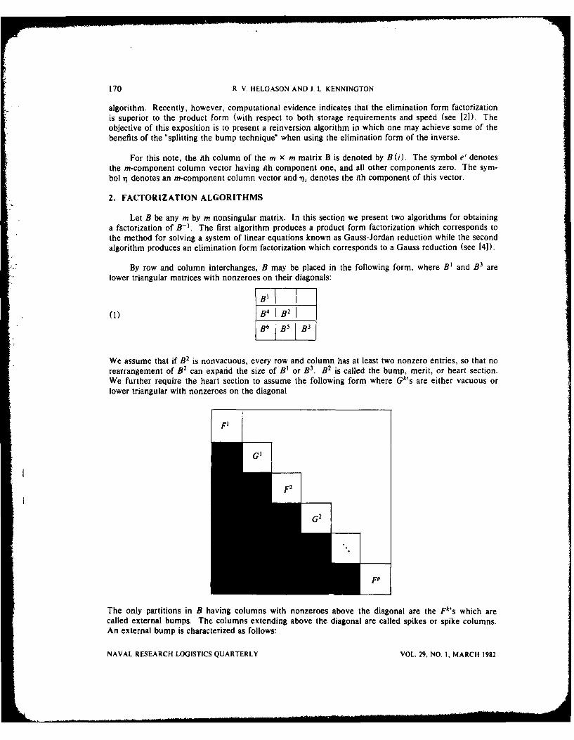
170 R. V. HELGASON AND J. L. KENNINGTON
algorithm. Recently, however, computational evidence indicates that the elimination form factorizationis superior to the product form (with respect to both storage requirements and speed (see (21). Theobjective of this exposition is to present a reinversion algorithm in which one may achieve some of thebenefits of the "splitting the bump technique" when using the elimination form of the inverse.
For this note, the ith column of the m x m matrix B is denoted by B (i). The symbol e' denotesthe m-component column vector having ith component one, and all other components zero. The sym-bol - denotes an m-component column vector and "i' denotes the ith component of this vector.
2. FACTORIZATION ALGORITHMS
Let B be any m by m nonsingular matrix. In this section we present two algorithms for obtaininga factorization of B-1 . The first algorithm produces a product form factorization which corresponds tothe method for solving a system of linear equations known as Gauss-Jordan reduction while the secondalgorithm produces an elimination form factorization which corresponds to a Gauss reduction (see [4]).
By row and column interchanges, B may be placed in the following form, where B' and B3 arelower triangular matrices with nonzeroes on their diagonals:
BiY
(1) B4 B. IB 6 B5 B3
We assume that if B2 is nonvacuous, every row and column has at least two nonzero entries, so that norearrangement of B 2 can expand the size of B1 or B 3. B 2 is called the bump, merit, or heart section.We further require the heart section to assume the following form where Gk's are either vacuous orlower triangular with nonzeroes on the diagonal
The only partitions in B having columns with nonzeroes above the diagonal are the Fk's which arecalled external bumps. The columns extending above the diagonal are called spikes or spike columns.An external bump is characterized as follows:
NAVAL RESEARCH LOGISTICS QUARTERLY VOL. 29, NO, I, MARCH 1982

SPLITTING BUMP IN FACTORIZATION 171
(i) the last column of an external bump will be a spike with a nonzero lying in the topmostrow of the external bump, and
(ii) the nonspike columns have nonzero diagonal elements.
The algorithms of Hellerman and Rarick (6, 71 produce such a structure for any nonsingular matrix B,and we shall call a matrix having this structure an HR matrix.
The product form factorization algorithm for an HR matrix is given as follows:
ALGORITHM 1: PRODUCT FORM FACTORIZATION FOR A HR MATRIX0. Initialization
Seti- 1 and A - B (1).1. Obtain New Eta
1I /A fork=1Set 7k - -3k/li, otherwise,
". fork=iand set Ei(k) - ek, otherwise.
(Note: only 7 and i need be saved in the ETA File rather than the matrix E')
2. Test For Termination
If i = m, terminate, otherwise, i - i + 1.
3. Test For Spike
If B(0) is not a spike, set/3 - B(i) and go to 1.
4. Spike Update
Let B(k) correspond to the first column of the external bump containing B(i). Set9 - E,-' ... EkBWi.
5. Swap Spikes If Pivot Element Equals Zero
If 3, ;d 0, go to 1, otherwise, there is some spike B(') in the same external bump havingj > isuch that the ith component of E -1 ... EkB() is nonzero. Set3 - EI- ... EkB(j),interchange B(i) and B(j) and go to 1.
In practice, the test for a zero pivot element in Step 5 is usually replaced by a tolerance test. LetTOL denote the tolerance to be used in the test. If I'3,1 < TOL, then 3, is treated as if it is zero. Dis-cussions of tolerances may be found in [12, 15, 161. Similar tolerance tests would ordinarily be incor-porated in the other algorithms to be presented in this exposition. To simplify the presentation theyhave been omitted here.
Justification for Algorithm I is given in [5]. At termination, B-1 - Em'E" - ... E'. Further-more, we see that for nonspike columns, each 3 and consequently each "l has exactly the same numberof nonzeroes as the corresponding column of B. However, the 'n for a spike column may have a higherdensity than the original column of B. The phenomena of an -q having a higher density than thecorresponding column of B is known as fill-in.
VOL. 29, NO, I, MARCH 1982 NAVAL RESEARCH LOGISTICS QUARTERLY
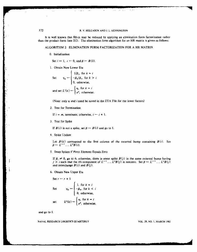
172 R. V. HELGASON AND J. L. KENNINGTON
It is well known that fill-in may be reduced by applying an elimination form factorization ratherthan the product form (see [11). The elimination form algorithm for an HR matrix is given as follows:
ALGORITHM 2: ELIMINATION FORM FACTORIZATION FOR A HR MATRIX
0. Initialization
Set i- 1, r-0,and3- B(1).
1. Obtain New Lower Eta
J 1/,3, for k = i
Set ' -- -Bk/1, for k > i
0, otherwise,
-q, fork = iand set L(k) - ke k, otherwise.
(Note: only q and i need be saved in the ETA File for the lower factors)
2. Test for Termination
If i = m, terminate; otherwise, i - i + 1.
3. Test for Spike
If B (i) is not a spike, set/3 - B () and go to 1.
4. Spike Update
Let B(k) correspond to the first column of the external bump containing B(i). SetjB - V - 1 ... L kB W).
5. Swap Spikes if Pivot Element Equals Zero
If 31 * 0, go to 6; otherwise, there is some spike B(1) in the same external bump havingj > i such that the ith component of L i-1 ... LkB(j) is nonzero. Set3 - L ... L"B(j)and interchange B (i) and B (j).
6. Obtain New Upper Eta
Set r - r + 1
S 1, fork=iSet Ilk "- --/3k, for k < i
0, otherwise,
17, fork - iset U'(k) ek, otherwise,
and go to 1.
NAVAL RESEARCH LOGISTICS QUARTERLY VOL. 29, NO. 1, MARCH 1982
I r .. ... .. . . . . . . 111 1 I I .. .. I ' I . . . . . .. . .. ..

SPLITTING BUMP IN FACTORIZATION 173
(Note: only -q and i need be saved in the ETA File for the upper factors). At the termination ofAlgorithm 2, B- 1 - U, ... ... L , where the upper eta's are upper triangular and the lower eta'sare lower triangular. As with Algorithm 1 fill-in has been restricted to the eta's corresponding to spikecolumns.
3. SPLITTING THE BUMP
In an attempt to reduce the fill-in which occurs in spike columns during a reinversion using Algo-rithm 1, a variation of the elimination form factorization algorithm (attributed to Martin Beale, see[131) has been used by some practitioners. This technique has been called "splitting the bump" after itstreatment of external bump columns.
Consider a set of columns of the basis corresponding to an external bump, say
nrows
p rows
where F is an external bump. Suppose F contains q spikes. If we apply the standard product form algo-rithm, we obtain a set of eta's such that
0
En... E'B 3 I n
0,
The eta's corresponding to the q spikes may incur fill-in. If we split the bump, the fill-in can be res-tricted to the n rows corresponding to F; hence, we may avoid fill-in in the last p rows. Since p may bemuch larger than n, the savings could be substantial. The price which must be paid to attain this reduc-tion in fill-in is that each external bump will require 2 n + q eta's rather than n. The savings in fill-in istypically so great that it offsets the additional storage which must be given up for the additional eta's.
The product form algorithm incorporating the "splitting the bump" technique is given as follows:
ALGORITHM 3: PRODUCT FORM FACTORIZATION FOR A HR MATRIXINCLUDING SPLITTING THE BUMP
0. Initialization
Set i - 1, j - 1, and P - B(I). If B(1) is in an external bump, go to 4.
1. Obtain New Lower Eta
1 7 /13,, for k - iSet " ---- /, otherwise,
I , fork- iand set Ej(k) - ek, otherwise.
Setj -j + 1.
VOL. 29. NO. I, MARCH 1982 NAVAL RESEARCH LOGISTICS QUARTERLY

174 R. V. HELGASON AND J. L. KENNINGTON
2. Test for Termination
If i - m, terminate; otherwise, i - i + I and P-- B(i).
3. Test for External Bump
If B () is not the first column in an external bump, go to 1.
4. Initialization for Bump
I - j (current length of Eta File)s - i (first column in this external bump)b - number of columns in this external bump
t - i + b - I (last column in this external bump)
5. Obtain Lower Eta
1/1,, fork =
Set 't k- -3k/13,, fori < k t
0, otherwise,
7), fork =and set EJ(k) - e, otherwise.
Setj.-j+ 1.
6. Test for End of Bump
Ifi = t, go to 10; otherwise, i - i + 1.
7. Test for Spike
If 8(B) is not a spike, set13 -- B(i) and go to 5.
8. Spike Update
Set#-- Ej- I... E(i).
9. Swap Spikes if Pivot Element Equals Zero
If P, ;d 0, go to 5; otherwise, there is some spike B(r) in the same external bump havingr > i such that the ith component of E - 1 ... E'B(r) is nonzero. Set s - E3- I ... E'B(r),interchange B(r) and B(i) and go to 5.
10. Obtain Upper Eta
1, fork= i
Set 71k -1k, fork < i
0, otherwise,
Iq, fork-,and set EJk -I ek, otherwise.
Set j - + 1 and i - i - I.
NAVAL RESEARCH LOGISTICS QUARTERLY VOL. 29. NO. 1, MARCH 1982

SPLITTING BUMP IN FACTORIZATION 175
11. Test for Beginning of Bump
If i = s, set A- B(i) and go to 13.
12. Test for Spike
If B(i) is not a spike, set i - i - 1 and go to 11; otherwise, set/3 - E - I ... E'B(i) andgo to 10.
13. Obtain Lower Eta
1, for k = i
Set 7'k -1 3 k, fork > t
0, otherwise,
J , fork= iand set Ej(k) - ek, otherwise.
Setj-j+ 1.
14. Test for End of Bump
If i = t, go to 2; otherwise i - i + 1, set3 6- B(i), and go to 13.
At the termination of Algorithm 3, B -1 = EJ-I ... El. Furthermore, all eta's are either upper triangu-lar or lower triangular, but they are intermixed.
Recall that Algorithm 2 produces a set of lower triangular factors followed by a set of upper tri-angular factors. If one incorporates the "splitting the bump" technique into Algorithm 2 and applies itto an HR matrix, the lower and upper factors become intermingled. Once the factors have becomeintermingled, we may no longer use the important algorithm of Forrest and Tomlin [2] to maintain theelimination form. We now show how one may achieve a partial "splitting of the bump" while simul-taneously maintaining a partitioning of the upper and lower factors.
Recall that an HR matrix takes the form given in (1).
By a rearrangement of rows and columns, the HR matrix (1) may be placed in the following form:
§3 g6 F?5
A- BI
B4 B2
u v w
VOL. 29, NO. 1, MARCH 1982 NAVAL RESEARCH LOGISTICS QUARTERLY

176 R. V. HELGASON AND J. L. KENNINGTON
where b 6 and B5 are row permutations of B 6 and B5, respectively, and B3 is a row and column permu-tation of B3. Applying a variation of Algorithm 2 to B eliminates all fill-in in B 5 while representing b-1as a product of upper factors followed by a product of lower factors. The details are given in the fol-lowing algorithm.
ALGORITHM 4: ELIMINATION FORM FACTORIZATION FOR A MODIFIED HR MATRIX
0. Initialization
Set i -u + 1 and - B(i). Ifv- 0, go to 3.
1. Obtain New Lower Eta
1/)9i, for k =
Set k for k > i
0, otherwise,
-q1, fork =and set L'(k) - Iek, otherwise.
2. Test for End of Section 2
Seti-i+ I and6-B(i). Ifi u+v, goto1. Ifw=0, goto8.
3. Obtain New Lower Eta
J 1/P,, for k = i
Set 7)k-- -3k/f3,' for k > i
0, otherwise,
J 7, forkand set L'(k) I ek. otherwise.
4. Test for End of Section 3
If i = m, go to 8; otherwise, i - i + I.
5. Test for Spike
If B(i) is not a spike, set/ -B(i) and go to 3.
6. Spike Update
Setf3 - Li-' ... Lu+'+B(i).
7. Swap Spikes if Pivot Element Equals Zero
If p, * 0, go to 3; otherwise, there is some spike B (j) in the same external bump havingj > i such that the ith component of L'-' ... Lu"+v+tB(J ) is nonzero. Set
-L'- ... Lu+v+ B(j), interchange B(i) and B(j) and go to 3.
NAVAL RESEARCH LOGISTICS QUARTERLY VOL, 29, NO. I, MARCH 1982

SPLITTING BUMP IN FACTORIZATION 177
8. Obtain New Upper Eta
1, fork = i
Set 7)k- --3 k, for k < i
0, otherwise,
I , fork = iand set U'(k) - ek, otherwise.
9. Check for End of Section 2
Set i - i - 1. If i = 0, terminate.If i = u, setf3 - B(G) and go to 12.
10. Set Column
If i > u + r, set13 - L'... Lu+v t B(i); otherwise,set # -B(i). Go to 8.
11. Obtain New Upper Eta
1/,3,, for k = i
Set "k --k/3, for k < i
0, otherwise,rfork A-
and set Ui(k) - e k, orieIek, otherwise.
12. Check for Termination
If i = 1, terminate; otherwise3 - B (i) and go to 11.
At the termination of Algorithm 4, 9-1 - U1 ... UmLm ... LU+I, and the fill-in has been restricted toB2. Hence, Algorithm 4 gains some of the benefits of the "splitting the bump" technique while main-taining a partitioning of the upper and lower factors. The benefits are not as great as with ordinary"bump splitting" since each individual external bump is split, whereas here the split is with respect tothe entire heart section.
A variation of Algorithm 4 has also been used by Tomlin (15]. Our contribution is that we have
tied together the ideas of "splitting the bump" in both the product and elimination form factorizationsand we have explicitly indicated via Algorithms 3 and 4 how these may be implemented.
REFERENCES
I]] Brayton, R.K., F.G. Gustavson and R.A. Willoughby, "Some Results on Sparse Matrices,"Mathematics of Computation, 24, 112, 937-954 (1970).
12] Forrest, J.J.H. and J.A. Tomlin, "Updated Triangular Factors of the Basis to Maintain Sparsity inthe Product from Simplex Method," Mathematical Programming, 2, 263-278 (1972).
13) Greenberg, HJ, and D.C. Rarick, "Determining GUB Sets Via an Invert Agenda Algorithm,"Mathematical Programming, 7, 240-244 (1974).
[41 Hadley, G., Linear Algebra (Addison Wesley Publishing Co., Inc., Reading, MA, 1964).
VOL. -9, NO. I, MARCH 1982 NAVAL RESEARCH LOGISTICS QUARTERLY
178 R. V. HELGASON AND J. L. KENNINGTON
[5] Helgason, R.V. and J.L. Kennington, "Spike Swapping in Basis Reinversion," Naval ResearchLogistics Quarterly, 27, 697-701 (1980).
[61 Hellerman, E. and D. Rarick, "Reinversion With the Preassigned Pivot Procedure," MathematicalProgramming, 1, 195-216 (1971).
(7] Hellerman, E. and D. Rarick, "The Partitioned Preassigned Pivot Procedure (p4 )," Sparse Matricesand Their Applications, Edited by D. Rose and R. Willoughby (Plenum Press, New York,1972).
[8] Kalan, J.E., "Aspects of Large-Scale In-Core Linear Programming," Proceedings of the ACM,304-313 (1971).
[9] Luhks, R.A., "Large-Scale Linear Programming Problems: Analysis and Generation," unpublisheddissertation, Department of Computer Science and Operations Research, Southern MethodistUniversity, Dallas, TX (1972).
[10] Marceau, I.W., R.J. Lermit, J.C. McMillan, T. Yamamoto and S.S. Yardley, "Linear Programmingon Illiac IV," Proceedings of Fourth Austrailian Computer Conference, Adelaide, Australia.481-485 (1969).
[111 Markowitz, H.M., "The Elimination Form of the Inverse and Its Application to Linear Program-ming," Management Science, 3, 255-269 (1975).
[12] Orchard-Hays, W., Advanced Linear-Programming Computing Techniques, (McGraw-Hill, New York,1968).
[131 Orchard-Hays, W., "An Exercise in Basis Inversion," SIGMAP Newsletter, No. 15 (1973).(141 Tomlin, J.A., "Modifying Triangular Factors of the Basis in the Simplex Method," in Sparse
Matrices and Their Applications, Edited by D.J. Rose and R.A. Willoughby (Plenum Press, NewYork, 1972).
[15] Tomlin, J.A., "Pivoting for Size and Sparsity in Linear Programming Inversion Routines," Journalof the Institute of Mathematics and its Applications, 10, 289-295 (1972).
[16] Tomlin, J.A., "An Accuracy Test for Updating Triangular Factors," Mathematical Programing Study4, 142-145 (1975).
[171 White, W.W., "A Status Report on Computing Algorithms for Mathematical Programming," Com-puting Surveys, 5, 135-166 (1973).
NAVAL RESEARCH LOGISTICS QUARTERLY VOL. 29, NO. t, MARCH 1982
A NOTE ON SOLVING MULTIFACILITY LOCATIONPROBLEMS INVOLVING EUCLIDEAN DISTANCES
Henrik Juel
Soenderborg School of Economics and Business AdministrationSoenderborg, Denmark
ABSTRACT
This note considers a recently proposed solution method for a multifacilitylocation problem. It is shown that the method does not always produce an op-timal solution.
In a recent issue of this journal Calamai and Charalambous [I conclude that many existingmethods designed for solving the multifacility location problem are either poorly structured, subop-timal, or haphazard (p. 619). It should be pointed out that their proposed algorithm belongs to thesame class of methods, in the sense that the algorithm sometimes gives a suboptimal solution.
The authors base their algorithm on a set of necessary conditions and seem to believe that this setof conditions is also sufficient for optimality, although sufficiency has yet to be proven (p. 617). In aproblem involving rectilinear distances the necessary conditions are also sufficient [3). This result holdsfor Euclidean distances, too, as long as each case of facility coincidence involves just two facilities [2].But if a current solution to a problem involving Euclidean distances has three or more facilities locatedat the same point, the author's set of necessary conditions are not in general sufficient for optimality, as
shown by the following example.
Consider a current solution where new facilities 1, 2, and 3 occupy the same location and no otherfacility occupies this location. Let the given weights relating to these new facilities be v12 = 1, v13 = 1,and v23 - 51/2 - 1. Suppose the other weights and facility locations are such that the pseudo-gradientsin (4.2c) (p. 613) are GI - (2, 0), G2 = (0, 1), and G3 = (-2, -1). Now consider the necessary con-ditions for optimality in (5.3) (p. 613). When S contains one element, the left hand sides of the condi-tion are 2, 1, and 51/2, whereas the right hand sides are 2, 51/2, and 51/2 Hence, moving one of thenew facilities 1., 2, or 3, as done in step (3) (p. 615) of the authors' algorithm, does not yield a bettersolution. Moving the entire cluster of these new facilities is likewise unsuccessful, since the sum of thepseudo-gradients is (0, 0). Finally, when S contains two elements, the conditions for S containing oneelement are repeated so moving a subset cluster, as done in step (5) of the algorithm, would not yield abetter solution,
Summarizing, the example represents a situation where the algorithm will stop, because thenecessary conditions for optimality are satisfied. But the current solution is suboptimal, because thedirectional derivative is not nonnegative for all directions. To verify this consider, for instance, a direc-tion vector D where the only nonvanishing two-dimensional component vectors are D1 - (-4, - 1) andD - (-2, -1). (D can be normalized into a unit vector by using the factor 221/2, if desired.) Thedirectional derivative at the current solution in this direction is given by (4.1) (p. 612), which yields:-8- 1 +0+ 2+ 171/2+ (5- 51/2), which is negative. Thus, a better solution can be achieved by keepingnew facility 3 fixed, and by moving new facilities I and 2, not as a subcluster, but along the separatedirections indicated above.
VOL. 29, NO. I, MARCH 1982 179 NAVAL RESEARCH LOGISTICS QUARTERLY
180 H. JUEL
The possibility that facilities may coincide renders the objective function in the multifacility loca-tion problem nondifferentiable, and, thus, difficult to handle computationally. Until a satisfactorynondifferentiable optimization technique has been developed, decision makers should continue to use adifferentiable approximation to their problem (unless the distances are rectilinear). The new algorithmis of dubious value to a decision maker interested in an optimal solution to the problem.
Finally, it might be pointed out that problem 6 (p. 618) can be solved by inspection using corol-lary 2 and corollary 1 in 141. The results in this reference offer the potential for reduction of practicalproblems by exploiting the special weight structure.
ACKNOWLEDG MENT
The author wishes to thank an anonymous referee, whose comments made significant improve-ments possible in the original manuscript.
REFERENCES
[D] Calamai, P. and C. Charalambous, "Solving Multifacility Location Problems Involving EuclideanDistances," Naval Research Logistics Quarterly, 27, 609-620 (1980).
[21 Juel, H., "Solution Conditions for Generalized Weber Problems with Two New Facilities," Transpor-tation Science (to appear).
[31 Juel, H. and R.F. Love, "An Efficient Computational Procedure for Solving the Multi-Facility Rec-tilinear Facilities Location Problem," Operational Research Quarterly, 27, 697-703 (1976).
[4] Juel, H. and R.F. Love, "Sufficient Conditions for Optimal Facility Locations to Coincide," Tran-sportation Science, 14, 125-129 (1980).
NAVAL RESEARCH LOGISTICS QUARTERLY VOL. 29. NO. 1, MARCH 1982

SUIBSCRIPTION Deposit AcutNme O FIEUEOLORDER FORM - un~ __ Chargri
I Enclosed
1 t.os~ fld Wr. or mflreo) orJ!e), or ckjqet to m y To be -ailed -
Smt-,,,ns'eJrnr of Docsu,,,o', Depo AIccou~nt Nkmbir iboun ab.o~e. Subscriptions -
I t 0 <Postaoe -
I ' = o~r~ror~r~~.~erForeign han'lhing - -
0 C.MMOB -
0C N Peale lend she juriu pfo, I katv MAIL ORDER FORM TO: ON~
*r h- oteodes hsno ~ S perintenderrt of Docusments - -UPNS
(u _*. oomothsfruS. Governm-enst Printing OfficeOs ut
= - 1 otmo htf Washsngton. D.C- 20402 Refund
I .0Credit Card Orders Only
Total charges$1FI ntebesblw
Card No. -- IEEE E E E
- )S Expirations DateLIT i
E NOTE: Complete top address Portion if dofferent from that at the bottom.
r- Name -------t----- ----to---------------------------------------------------ZPcc
I C ) Stee Ad s -- - - - - - - - - - - - - - - - - - - - -- I- - -- -- - - - -- - - -
NRLQ aandeeac Logitic Quarte--- - -- - - -- --- - - -- --ly- -- - - ZIP Coc--- -- -
0 111110 TITL PRICE
* so
E
IC
ItIt-
I 4. COMPANY OR PERSONAL NAME
0 ~ADDITIONAL ADDRESS/ATTENTION LIN
-U STREET ADDRESS
0
f- ., ICITY STAE IP 7J
I I (or) COUNTRY
I PLEASE PRINT
INFORMATION FOR CONTRIBUTORS
The NAVAL RESEARCH LOGISTICS QUARTERLY is devoted to the dissemination ofscientific information in logistics and will publish research and expository papers, including thosein certain areas of mathematics, statistics, and economics, relevant to the over-all effort to improvethe efficiency and effectiveness of logistics operations.
Manuscripts and other items for publication should be sent to The Managing Editor, NAVALRESEARCH LOGISTICS QUARTERLY, Office of Naval Research, Arlington, Va. 22217.Each manuscript which is considered to be suitable material tor the QUARTERLY is sent to oneor more referees.
Manuscripts submitted for publication should be typewritten, double-spaced, and the authorshould retain a copy. Refereeing may be expedited if an extra copy of the manuscript is submittedwith the original.
A short abstract (not over 400 words) should accompany each manuscript. This will appearat the head of the published paper in the QUARTERLY.
There is no authorization for compensation to authors for papers which have been acceptedfor publication. Authors will receive 250 reprints of their published papers.
Readers are invited to submit to the Managing Editor items of general interest in the fieldof logistics, for possible publication in the NEWS AND MEMORANDA or NOTES sectionsof the QUARTERLY.

NAVAL RESEARCH MARCH 1982 *
LOGISTICS VOL. 29. NO. 1QUARTERLY NAVSO P-1278
CONTENTSARTICLES Page
A Theory of Multistage Contractual Incentives R.W. BLANNING 1with Application to Design-to-Cost P.R. KLEINDORFER
C.S. SANKAR
Optimal Strategies in a Game of Economic Survival K. BORCH 19
Diagnostic Analysis of Inventory Systems: an G.R. BITRAN 29Optimization Approach A.C. HAX
J. VALOR-SABATIER
Production Planning for Multi-Resource R.C. LEACHMAN 47Network Systems
The Class of MIFRA Lifetimes and Its H.W. BLOCK 55Relation to Other Classes T.H. SAVITS
Remarks on a Univariate Shock Model with W.S. GRIFFITH 63Some Bivariate Generalizations
Asymptotic Joint Normality of an Increasing L. WEISS 75Number of Multivariate Order Statisticsand Associated Cell Frequencies
Minimizing Costs of Sequential and Parallel P.D. FEIGIN 87Personnel Testing Programs G.H. HAREL
The Variance of the Coverage of a Randomly G. SCHROETER 97Located Area Target by a Salvo of Weapons
Reformulating Zero-Sum Games with E.L. HANNAN 113Multiple Goals
On a Generalized Bin-Packing Problem R.T. LEWIS 119R.G. PARKER
An Integer Programming Algorithm for M.W. COOPER 147Portfolio Selection with Fixed Charges K. FARHANGIAN
Scheduling of a Single Machine to L. BIANCO 151Minimize Total Weighted Completion S. RICCIARDELLITime Subject to Release Dates
A Note on Splitting the Bump in an R.V. HELGASON 169Elimination Factorization J.L. KENNINGTON
A Note on Solving Multifacility Location H. JUEL 179Problems Involving Euclidean Distances
OFFICE OF NAVAL RESEARCHArlington, Va. 22217