Ad Hoc and Sensor Networks – Roger Wattenhofer –1/1Ad Hoc and Sensor Networks – Roger Wattenhofer –1/1 Introduction Chapter 1

Ad Hoc and Sensor Networks – Roger Wattenhofer – 1/1Ad Hoc and Sensor Networks – Roger Wattenhofer – 1/1

IntroductionChapter 1

Power

Processor

Radio

SensorsMemory

Today, we look much cuter!

And we’re usually carefully deployed


A Typical Sensor Node: TinyNode 584

• TI MSP430F1611 microcontroller @ 8 MHz

• 10k SRAM, 48k flash (code), 512k serial storage

• 868 MHz Xemics XE1205 multi channel radio

• Up to 115 kbps data rate, 200m outdoor range

[Shockfish SA, The Sensor Network Museum]

Current Draw

Power Consumption

uC sleep with timer on 6.5 uA 0.0195 mW

uC active, radio off 2.1 mA 6.3 mW

uC active, radio idle listening 16 mA 48 mW

uC active, radio TX/RX at +12dBm

62 mA 186 mW

Max. Power (uC active, radio TX/RX at +12dBm + flash write)

76.9 mA 230.7mW


After Deployment

multi-hop communication

Visuals anyone?

Ad Hoc and Sensor Networks – Roger Wattenhofer – 1/6

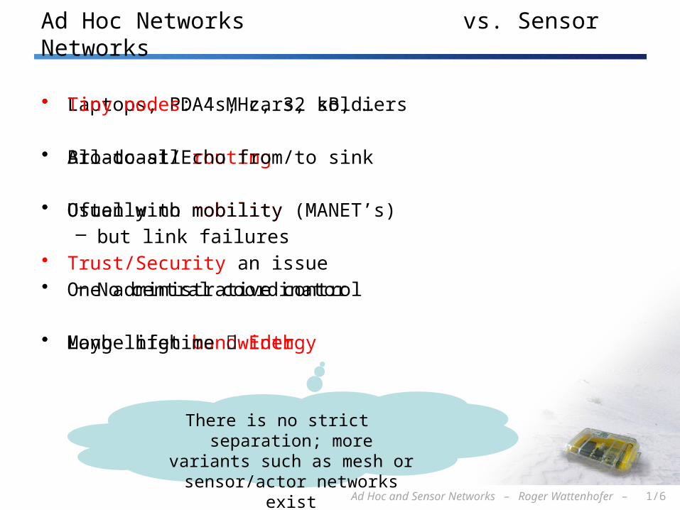
Ad Hoc Networks vs. Sensor Networks

• Laptops, PDA’s, cars, soldiers

• All-to-all routing

• Often with mobility (MANET’s)

• Trust/Security an issue– No central coordinator

• Maybe high bandwidth

• Tiny nodes: 4 MHz, 32 kB, …

• Broadcast/Echo from/to sink

• Usually no mobility– but link failures

• One administrative control

• Long lifetime Energy

There is no strict separation; more variants such as mesh or

sensor/actor networks exist


Overview

• Introduction• Application Examples• Related Areas• Course Overview• Literature

• For CS Students: Wireless Communication Basics• For EE Students: Network Algorithms Overview


Animal Monitoring (Great Duck Island)

1. Biologists put sensors in underground nests of storm petrel

2. And on 10cm stilts 3. Devices record data about birds4. Transmit to research station5. And from there via satellite to lab


Environmental Monitoring (Redwood Tree)

• Microclimate in a tree• 10km less cables on a tree; easier to set up• Sensor Network = The New Microscope?


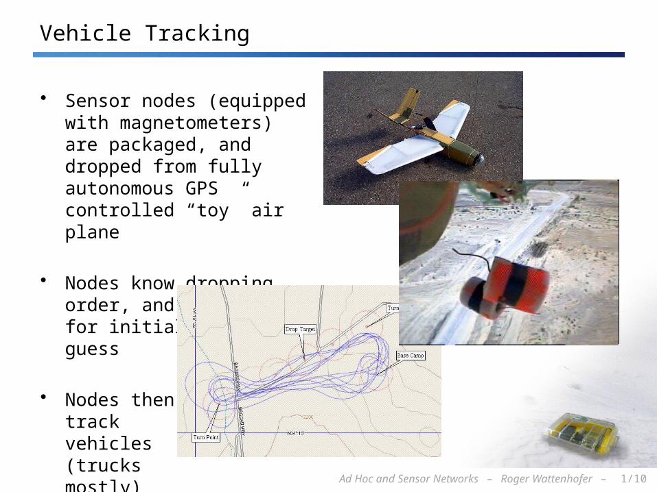
Vehicle Tracking

• Sensor nodes (equipped with magnetometers) are packaged, and dropped from fully autonomous GPS controlled “toy” air plane

• Nodes know dropping order, and use that for initial position guess

• Nodes thentrack vehicles(trucksmostly)

Smart Spaces (Car Parking)

• The good: Guide cars towards empty spots

• The bad: Check which cars do not have any time remaining

• The ugly: Meter running out: take picture and send fine

Turn right!50m to go…

Park!

Turn left!30m to go…

[Matthias Grossglauser, EPFL & Nokia Research]


Structural Health Monitoring (Bridge)

Detect structural defects, measuring temperature, humidity, vibration, etc.

Swiss Made [EMPA]


Virtual Fence (CSIRO Australia)

• Download the fence to the cows. Today stay here, tomorrow go somewhere else.

• When a cow strays towards the co-ordinates, software running on the collar triggers a stimulus chosen to scare the cow away, a sound followed by an electric shock; this is the “virtual” fence. The software also "herds" the cows when the position of the virtual fence is moved.

• If you just want to make sure that cows stay together, GPS is not really needed…

Cows learn and need not to be shocked

later… Moo!


Economic Forecast

• Industrial Monitoring (35% – 45%)• Monitor and control production chain• Storage management• Monitor and control distribution

• Building Monitoring and Control (20 – 30%)• Alarms (fire, intrusion etc.)• Access control

• Home Automation (15 – 25%)• Energy management (light, heating, AC etc.)• Remote control of appliances

• Automated Meter Reading (10-20%)• Water meter, electricity meter, etc.

• Environmental Monitoring (5%)• Agriculture• Wildlife monitoring

0

100

200

300

400

500

600

millions wireless sensors sold

[Jean-Pierre Hubaux, EPFL]


Related Areas

Ad Hoc & Sensor

Networks

RFID

…

MobileWireless

Wearable


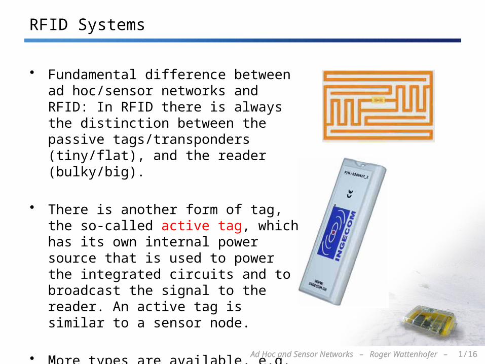
RFID Systems

• Fundamental difference between ad hoc/sensor networks and RFID: In RFID there is always the distinction between the passive tags/transponders (tiny/flat), and the reader (bulky/big).

• There is another form of tag, the so-called active tag, which has its own internal power source that is used to power the integrated circuits and to broadcast the signal to the reader. An active tag is similar to a sensor node.

• More types are available, e.g. the semi-passive tag, where the battery is not used for transmission (but only for computing)


Wearable Computing / Ubiquitous Computing

• Tiny embedded “computers”• UbiComp: Microsoft’s Doll

• I refer to my colleagueGerhard Troester andhis lectures & seminars

[Schiele, Troester]


Wireless and/or Mobile

• Aspects of mobility– User mobility: users communicate “anytime, anywhere, with anyone”

(example: read/write email on web browser)– Device portability: devices can be connected anytime, anywhere to the

network• Wireless vs. mobile Examples

Stationary computer Notebook in a hotel Historic buildings; last mile Personal Digital Assistant (PDA)

• The demand for mobile communication creates the need for integration of wireless networks and existing fixed networks– Local area networks: standardization of IEEE 802.11 or HIPERLAN– Wide area networks: GSM and ISDN – Internet: Mobile IP extension of the Internet protocol IP


Wireless & Mobile Examples

• Up-to-date localized information– Map– Pull/Push

• Ticketing• Etc.

[Asus PDA, iPhone, Blackberry, Cybiko]


General Trend: A computer in 10 years?

• Advances in technology– More computing power in smaller devices– Flat, lightweight displays with low power consumption– New user interfaces due to small dimensions– More bandwidth (per second? per space?)– Multiple wireless techniques

• Technology in the background– Device location awareness: computers adapt to their environment– User location awareness: computers recognize the location of the

user and react appropriately (call forwarding)• “Computers” evolve

– Small, cheap, portable, replaceable– Integration or disintegration?


Physical Layer: Wireless Frequencies

1 Mm300 Hz

10 km30 kHz

100 m3 MHz

1 m300 MHz

10 mm30 GHz

100 m3 THz

1 m300 THz

visible lightVLF LF MF HF VHF UHF SHF EHF infrared UV

twisted pair coax

AM SW FM

regulated

ISM


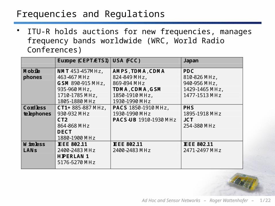
Frequencies and Regulations

• ITU-R holds auctions for new frequencies, manages frequency bands worldwide (WRC, World Radio Conferences)

Europe (CEPT/ETSI) USA (FCC) Japan

Mobile phones

NMT 453-457MHz, 463-467 MHz GSM 890-915 MHz, 935-960 MHz, 1710-1785 MHz, 1805-1880 MHz

AMPS, TDMA, CDMA 824-849 MHz, 869-894 MHz TDMA, CDMA, GSM 1850-1910 MHz, 1930-1990 MHz

PDC 810-826 MHz, 940-956 MHz, 1429-1465 MHz, 1477-1513 MHz

Cordless telephones

CT1+ 885-887 MHz, 930-932 MHz CT2 864-868 MHz DECT 1880-1900 MHz

PACS 1850-1910 MHz, 1930-1990 MHz PACS-UB 1910-1930 MHz

PHS 1895-1918 MHz JCT 254-380 MHz

Wireless LANs

IEEE 802.11 2400-2483 MHz HIPERLAN 1 5176-5270 MHz

IEEE 802.11 2400-2483 MHz

IEEE 802.11 2471-2497 MHz


Course Overview

Application

Transport

Network

Link

Physical 1 Basics

1 Applications

2 Geo-Routing

3 Topology Control

13 Mobility 4 Data Gathering

10 Clustering

9 Positioning8 Clock Sync

6 MAC Practice

12 Routing

14 Transport

11 Capacity

Practice Theory

5 Network Coding

7 MAC Theory


Course Overview: Lecture and Exercises

• Maximum possible spectrum of theory and practice• New area, more open than closed questions• Each week, exactly one topic (chapter)

• General ideas, concepts, algorithms, impossibility results, etc.– Most of these are applicable in other contexts– In other words, almost no protocols

• Two types of exercises: theory/paper, practice/lab• Assistants: Philipp Sommer, Johannes Schneider

• www.disco.ethz.ch courses


Literature


More Literature

• Bhaskar Krishnamachari – Networking Wireless Sensors• Paolo Santi – Topology Control in Wireless Ad Hoc and Sensor

Networks• F. Zhao and L. Guibas – Wireless Sensor Networks: An Information

Processing Approach• Ivan Stojmeniovic – Handbook of Wireless Networks and Mobile

Computing • C. Siva Murthy and B. S. Manoj – Ad Hoc Wireless Networks• Jochen Schiller – Mobile Communications• Charles E. Perkins – Ad-hoc Networking• Andrew Tanenbaum – Computer Networks

• Plus tons of other books/articles• Papers, papers, papers, …


Rating (of Applications)

• Area maturity

• Practical importance

• Theory appeal

First steps Text book

No apps Mission critical

Boooooooring Exciting


Open Problem

• Well, the open problem for this chapter is obvious:

• Find the killer application! Get rich and famous!!

…this lecture is only superficially about ad hoc and sensor

networks. In reality it is about new (and hopefully exciting) networking paradigms!


For CS Students: Wireless Communication Basics

• Brief history of communication• Frequencies• Signals• Antennas• Signal Propagation• Modulation


A brief history of communication

• Electric telegraph invented in 1837 by Samuel Morse• First long distance transmission between Washington,

D.C. and Baltimore, Maryland in 1844: «What hath God wrought»

• Invention of the telephone by Alexander Graham Bell in 1875

Going Wireless

• Guglielmo Marconi demonstrates first wireless telegraph in 1896.

• A wireless telegraph service is established betweenFrance and England in 1898.

• 1901 first wireless communication accross the atlantic

• First amplitude modulation (AM) radio transmissionin 1906

• Edwin Howard Armstrong inventsfrequency modulation (FM) radio in 1935

• Digital Audio Broadcasting (DAB) since late 90’s


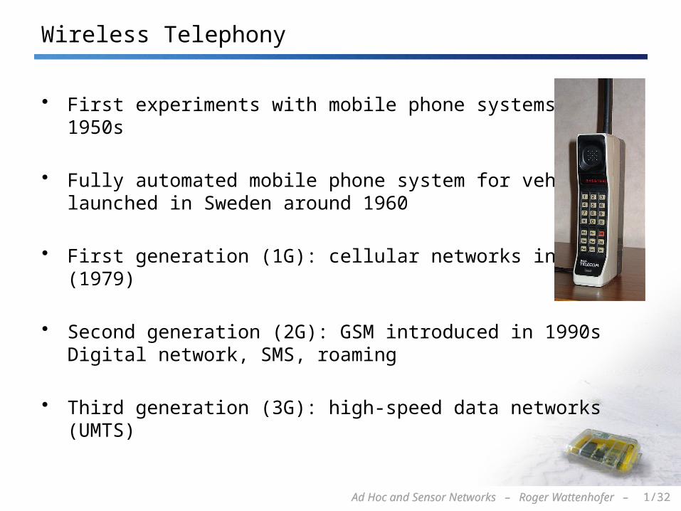
Wireless Telephony

• First experiments with mobile phone systems in 1950s

• Fully automated mobile phone system for vehicleslaunched in Sweden around 1960

• First generation (1G): cellular networks in Japan (1979)

• Second generation (2G): GSM introduced in 1990sDigital network, SMS, roaming

• Third generation (3G): high-speed data networks (UMTS)

Receiver

Transmitter

Block Diagram of a Wireless Communication System

• Modulation is required to transfer data over a wireless channel

Data In

Data Out

Modulator Antenna

AntennaDemodulator

Wireless Channel


Modulation and demodulation

synchronizationdecision

digitaldataanalog

demodulation

radiocarrier

analogbaseband

signal

101101001 radio receiver

digitalmodulation

digitaldata analog

modulation

radiocarrier

analogbaseband

signal

101101001 radio transmitter

• Modulation in action:


Periodic Signals

• g(t) = At sin(2π ft t + φt)

• Amplitude A• frequency f [Hz = 1/s]• period T = 1/f• wavelength λ

with λf = c (c=3∙108 m/s)

• phase φ

• φ* = -φT/2π [+T]

T

A0 t

φ*


• For many modulation schemes not all parameters matter.

Different representations of signals

f [Hz]

A [V]

R = A cos

I = A sin

*

A [V]

t [s]

amplitude domain frequency spectrum phase state diagram


Digital modulation

• Modulation of digital signals known as Shift Keying

• Amplitude Shift Keying (ASK):– very simple– low bandwidth requirements– very susceptible to interference

• Frequency Shift Keying (FSK):– needs larger bandwidth

• Phase Shift Keying (PSK):– more complex– robust against interference

1 0 1

t

1 0 1

t

1 0 1

t


Advanced Phase Shift Keying

• BPSK (Binary Phase Shift Keying):– bit value 0: sine wave– bit value 1: inverted sine wave– Robust, low spectral efficiency– Example: satellite systems

• QPSK (Quadrature Phase Shift Keying):– 2 bits coded as one symbol– symbol determines shift of sine wave– needs less bandwidth compared to BPSK– more complex

I

R01

I

R

11

01

10

00


Modulation Combinations

• Quadrature Amplitude Modulation (QAM)

• combines amplitude and phase modulation• it is possible to code n bits using one symbol• 2n discrete levels, n=2 identical to QPSK• bit error rate increases with n, but less errors compared to

comparable PSK schemes

• Example: 16-QAM (4 bits = 1 symbol)• Symbols 0011 and 0001 have the

same phase, but different amplitude. 0000 and 1000 have different phase, but same amplitude.

• Used in 9600 bit/s modems

0000

0001

0011

1000

I

R

0010


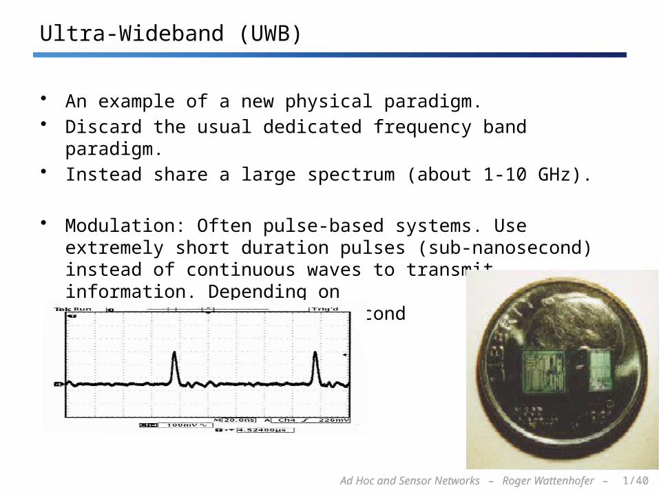
Ultra-Wideband (UWB)

• An example of a new physical paradigm.• Discard the usual dedicated frequency band paradigm. • Instead share a large spectrum (about 1-10 GHz).

• Modulation: Often pulse-based systems. Use extremely short duration pulses (sub-nanosecond) instead of continuous waves to transmit information. Depending on application 1M-2G pulses/second


UWB Modulation

• PPM: Position of pulse

• PAM: Strength of pulse

• OOK: To pulse or not to pulse

• Or also pulse shape


• Radiation and reception of electromagnetic waves, coupling of wires to space for radio transmission

• Isotropic radiator: equal radiation in all three directions• Only a theoretical reference antenna• Radiation pattern: measurement of radiation around an antenna• Sphere: S = 4π r2

Antennas: isotropic radiator

yz

xIdeal isotropic radiator


Antennas: simple dipoles

• Real antennas are not isotropic radiators but, e.g., dipoles with lengths /2 as Hertzian dipole or /4 on car roofs or shape of antenna proportional to wavelength

• Example: Radiation pattern of a simple Hertzian dipole

side view (xz-plane)

x

z

side view (yz-plane)

y

z

top view (xy-plane)

x

y

simpledipole

/4 /2


Antennas: directed and sectorized

side (xz)/top (yz) views

x/y

z

side view (yz-plane)

x

y

top view, 3 sector

x

y

top view, 6 sector

x

y

• Often used for microwave connections or base stations for mobile phones (e.g., radio coverage of a valley)

directedantenna

sectorizedantenna

[Buwal]


Antennas: diversity

• Grouping of 2 or more antennas– multi-element antenna arrays

• Antenna diversity– switched diversity, selection diversity

– receiver chooses antenna with largest output– diversity combining

– combine output power to produce gain– cophasing needed to avoid cancellation

• Smart antenna: beam-forming, MIMO, etc.

+

/4/2/4

ground plane

/2/2

+

/2


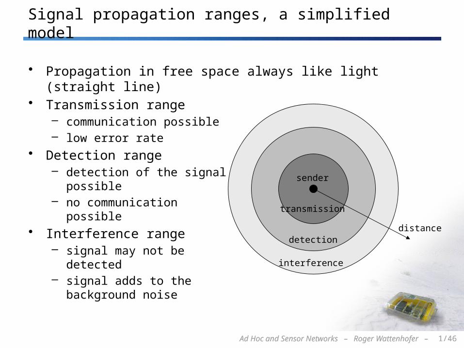
Signal propagation ranges, a simplified model

distance

sender

transmission

detection

interference

• Propagation in free space always like light (straight line)• Transmission range

– communication possible– low error rate

• Detection range– detection of the signal

possible– no communication

possible• Interference range

– signal may not be detected

– signal adds to the background noise


Pr =PsGsGr ¸2

(4¼)2d2L

Pr =PsGsGr h2

sh2r

d4

Signal propagation, more accurate models

• Free space propagation

• Two-ray ground propagation

• Ps, Pr: Power of radio signal of sender resp. receiver

• Gs, Gr: Antenna gain of sender resp. receiver (how bad is antenna)

• d: Distance between sender and receiver• L: System loss factor• ¸: Wavelength of signal in meters• hs, hr: Antenna height above ground of sender resp. receiver

• Plus, in practice, received power is not constant („fading“)


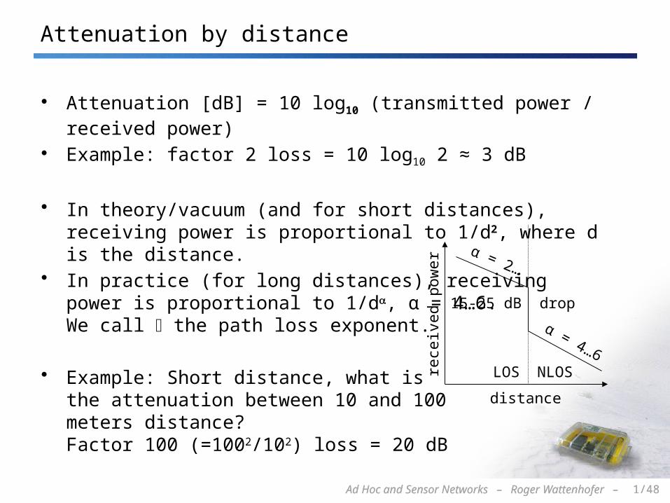
Attenuation by distance

• Attenuation [dB] = 10 log10 (transmitted power / received power)

• Example: factor 2 loss = 10 log10 2 ≈ 3 dB

• In theory/vacuum (and for short distances), receiving power is proportional to 1/d2, where d is the distance.

• In practice (for long distances), receiving power is proportional to 1/d, α = 4…6.We call the path loss exponent.

• Example: Short distance, what isthe attenuation between 10 and 100meters distance?Factor 100 (=1002/102) loss = 20 dB distance

rece

ived

pow

er

α = 2…

LOS NLOS

α = 4…6

15-25 dB drop


Attenuation by objects

• Shadowing (3-30 dB): – textile (3 dB)– concrete walls (13-20 dB)– floors (20-30 dB)

• reflection at large obstacles• scattering at small obstacles• diffraction at edges• fading (frequency dependent)

reflection scattering diffractionshadowing


• Signal can take many different paths between sender and receiver due to reflection, scattering, diffraction

• Time dispersion: signal is dispersed over time• Interference with “neighbor” symbols: Inter Symbol Interference (ISI)• The signal reaches a receiver directly and phase shifted• Distorted signal depending on the phases of the different parts

Multipath propagation

signal at sendersignal at receiver


Effects of mobility

• Channel characteristics change over time and location – signal paths change– different delay variations of different signal parts– different phases of signal parts

• quick changes in power received (short term fading)

• Additional changes in– distance to sender– obstacles further away

• slow changes in average power received (long term fading)

• Doppler shift: Random frequency modulation

short term fading

long termfading

t

power


Real World Examples


For EE Students: Network Algorithms Basics

• A Motivating Example: Steiner Tree• Complexity and Hardness• Approximation Algorithms• Minimum Spanning Tree

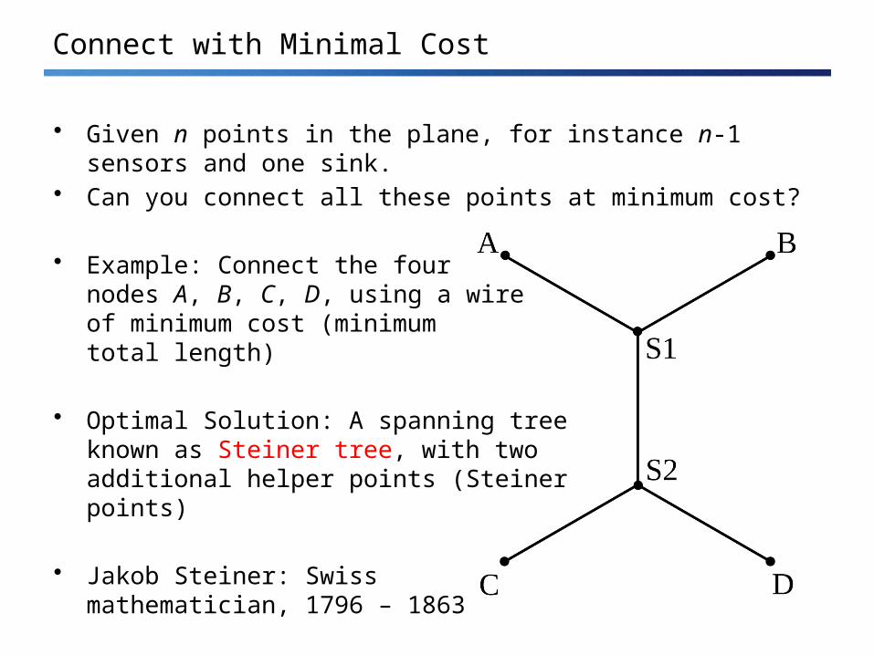
Connect with Minimal Cost

• Given n points in the plane, for instance n-1 sensors and one sink.• Can you connect all these points at minimum cost?

• Example: Connect the fournodes A, B, C, D, using a wireof minimum cost (minimumtotal length)

• Optimal Solution: A spanning tree known as Steiner tree, with two additional helper points (Steiner points)

• Jakob Steiner: Swiss mathematician, 1796 – 1863

Steiner Tree Facts

• It is known that Steiner points must have a degree of 3, and that the three edges incident to such a point must form three 120 degree angles.

• It follows that the maximum number of Steiner points that a Steiner tree can have is n − 2, where n is the initial number of given points.

• How can we compute the optimal Steiner tree?

Time Complexity

• The time complexity of an algorithm quantifies the amount of time taken by an algorithm to run as a function of the size of the input to the problem, e.g. time = 5n3 + 17n – 2.

• Time complexity is commonly computed by simply counting the number of elementary operations (such as additions or multiplications) performed by the algorithm, where an elementary operation takes a one time unit.

• Often multiplicative constants and lower order terms are suppressed, and the answer is given in “big Oh” notation, e.g. 5n3 + 17n – 2 = O(n3).

• Since an algorithm may take a different amount of time even on inputs of the same size, one commonly focuses on the so-called worst-case time complexity, the maximum amount of time taken on any (including the worst) input of size n.

Hardness

• A time complexity which is polynomial in the input is usually considered feasible, e.g. O(n1000) is okay.

• An algorithm becomes problematic if its time complexity is not polynomial anymore, e.g. exponential such as O(1.1n).

• In this example the first function may look scarier than the second, but for large enough n, the second function is much larger (well, after all it grows exponentially).

• In layman’s terms, if a problem is NP-hard, then it is a “difficult” problem. For problems that are NP-hard it is generally believed that there is no polynomial time algorithm which can solve the problem. However, this is just a conjecture. If you can proof it, you get very famous.

• The Steiner tree problem is known to be NP-hard.

What can one do if a problem is hard?

• If you are lazy, you may take it as a excuse to propose a heuristic (an algorithm without quality guarantees).

• Another way to go is to propose so-called fixed parameter algorithms. Some algorithms with exponential running time are still much better than others, e.g. O(1.1n) is much faster than O(nn) or O(n!)

• A very popular alternative is to propose so-called approximation algorithms. These are polynomial-time algorithms which cannot guarantee to find the optimum, but they can guarantee to find a solution which is at most a factor c worse than the (unknown) optimum.

• Is there an approximation algorithm for the Steiner tree problem?

Steiner Tree Approximations?

• What if you connect all the nodes directly to some arbitrarily chosen (root) node?– How much worse than the optimum solution will this be?

• Alternatively we might connect the nodes with the minimum cost spanning tree that does not use additional (Steiner) points. Such a spanning tree is known as the Minimum Spanning Tree (MST).– How can we compute such an MST?– How much worse than the optimum solution will this be?

• Indeed, for the Euclidean Steiner Tree problem there is even a polynomial-time approximation scheme (PTAS). This means that one can approximate the optimal solution up to a factor 1+ε, for an arbitrarily small ε > 0. However, the running time will grow as a function of ε.

Minimum Spanning Tree

• There are several simple algorithms that can compute the MST quickly. For instance the following:

• Choose the closest two nodes which are not yet connected (through a path) and connect them, until all nodes are connected by a spanning tree.

• Exercise: Proof that this is optimal.

Documents

Ad Hoc and Sensor Networks – Roger Wattenhofer –1/1Ad Hoc and Sensor Networks – Roger Wattenhofer –1/1 Introduction Chapter 1