Ad Hoc Wireless Networks (A Communication-Theoretic Perspective) || Effective Transport Capacity in Ad Hoc Wireless Networks

Chapter 5

Effective Transport Capacity inAd Hoc Wireless Networks

5.1 Introduction

Ad hoc wireless networks represent a new and exciting communication paradigm which couldhave multiple applications in future wireless communication systems. In particular, over thelast few years routing issues in ad hoc wireless networks, such as routing in the presence ofnode mobility [4,5,9,42,117] or energy consumption-aware routing [35,37–39,46,118,119],have been studied extensively. While routing is fundamental in ad hoc wireless networks,the approach taken by most recent studies is such that physical layer limitations are notconsidered. This approach is meaningful in networks where links are basically error-free(such as the Internet), but it could be misleading in wireless networks, where the reliabilityof radio links might be very limited.

Fundamental performance limits of such a communication paradigm need to be studied.The concept of transport capacity has been introduced in order to quantify the maximumachievable bandwidth–distance product which can be supported by the network. In [16],the authors compute the transport capacity of stationary wireless networks, considering twopossible models where inter-node interference (INI) is not taken into account: these aredefined as a protocol model (in this case, a transmission between two nodes is error-free,provided that their distance is suitably lower than the distance from the destination nodeto any of the other nodes in the network) and a physical model (in this case, error-freetransmission between two neighboring nodes is guaranteed if the signal-to-noise ratio, SNR,at the receiving node is above a specific threshold). Moreover, in [16] the authors distinguishbetween arbitrary networks – where the locations of nodes, destinations of sources and trafficdemands are all arbitrary – and random networks – where the nodes and their destinationsare randomly chosen. From the results in [16], it is possible to conclude that using a physicalmodel without interference, an upper bound on the transport capacity for a stationary wirelessnetwork with free-space path loss is �(Rb

√AN), where Rb is the channel data-rate of a node,

Ad Hoc Wireless Networks: A Communication-Theoretic Perspective Ozan K. Tonguz and Gianluigi Ferrari© 2006 John Wiley & Sons, Ltd. ISBN: 0-470-09110-X

112 Chapter 5. Effective Transport Capacity in Ad Hoc Wireless Networks

A is the network area and N is the number of nodes in the network.26 The capacity of ad hocwireless networks is also evaluated, in various scenarios and under various assumptions,in [120–129].

We point out that several of the results in this chapter will be obtained under specificassumptions regarding the network topology. In this sense, the reader has to assume that theclosed-form expressions provided in the following are exact ‘on the order’, and, as such, alsoprovide useful guidelines to the design of ad hoc wireless networks for other scenarios.

While the considered information-theoretic approach is interesting and provides ultimateachievable limits, the influence of physical layer characteristics and the medium accesscontrol (MAC) protocol on the achievable performance is not clear. In [130], the influence ofthe MAC protocol on the capacity of ad hoc wireless networks is considered in the particularcase of 802.11-type wireless networks. The theoretical framework developed for multi-hopad hoc wireless networks in Chapters 2 and 3 clearly shows how physical and MAC layers areinterrelated. In this chapter, we study the relation of the transport capacity with the used MACprotocol and the physical layer characteristics. In order to achieve our goal, we first introducethe concept of effective transport capacity in ad hoc wireless networks, representing the rate–distance product ‘actually’ carried by the network. We then develop a simple and intuitiveapproach for its evaluation in the case of packetized wireless communications over disjointmulti-hop routes. In the case of stationary nodes and no INI, the results predicted by ourtheoretical framework are in good agreement with the results obtained in [16] in the case ofan arbitrary network under the physical model without interference. Considering a realisticnetwork communication scenario with INI, two reservation-based MAC protocols suitablefor ad hoc wireless networks are considered: they are defined as reserve-and-go (RESGO)and reserve-listen-and-go (RESLIGO), respectively. The basic principles of operation ofboth MAC protocols are provided, and their performance is evaluated and compared tothat in the ideal case. It is shown that for low traffic load the RESGO MAC protocolguarantees an effective transport capacity identical to that in the ideal case, whereas theeffective transport capacity supported with the RESLIGO MAC protocol is lower. However,the overall maximum of the effective transport capacity with the latter MAC protocol islarger than that with the former MAC protocol. We show that the use of spreading codes,together with the RESGO MAC protocol, can significantly increase the system performance,i.e. improve the effective transport capacity. In this chapter, we will consider a communicationscenario characterized by a strong line of sight (LOS). The interested reader can extend theproposed analysis to other communication scenarios (e.g. the presence of a strong multipath)by following the approach outlined in Chapters 2 and 3.

The remainder of this chapter is organized as follows. In section 5.2, the basic assump-tions behind the considered network communication model are outlined. In section 5.3,communication-theoretic preliminaries are presented. In section 5.4, the concept of single-route effective transport capacity is introduced, while in section 5.5 the aggregate effectivetransport capacity is evaluated. In section 5.6, a comparative analysis of the considered MACprotocols is presented, and the obtained results are discussed. In section 5.7, an improvedversion of the RESGO MAC protocol, based on the use of per-route spreading codes, isproposed. A few observations on the obtained results are made in section 5.8, and Section 5.9concludes this chapter.

26The notation �(·) is used, in the realm of algorithms, to describe the asymptotic functional relationship betweenfunctions of time [17]. More precisely, the notation f (n) = �(g(n)) means that there exists an n0 such that, forn ≥ n0, ∃c1 ∈ (0, 1), c2 > 1 such that c1g(n) ≤ f (n) ≤ c2g(n).

5.2. Model and Assumptions 113

5.2 Model and AssumptionsIn the following, we outline the basic assumptions behind the network communication modelwhich will be used in the remainder of this chapter – note that several of these assumptionshave already been considered in the previous chapter.

• Peer-to-peer (P2P) wireless communications with disjoint multi-hop routes areconsidered. A source node, in need of communicating with a destination node,first reserves a series of intermediate relay nodes which constitute a multi-hopcommunication route to the destination. After the route has been created, the sourcenode activates the route. The activation instant depends on the MAC protocol.

• Static networks with regular lattice node distribution are considered. The extension ofthe proposed analysis to the case of a random topology can be considered following theapproach proposed in [41]. However, we note that the results presented in the followingare, on the order, valid also for a scenario with a random topology.

• Different multi-hop routes are assumed to be disjoint. In particular, a node cannot serveas a relay in more than one route – this aspect will be discussed in more detail insection 5.8.

• We do not consider how to build and maintain a route in this chapter. In otherwords, we assume that route creation is accomplished under ideal conditions. Althoughthis is a fundamental aspect of ad hoc wireless networking [4], our focus is on thecharacterization of the information transfer in operative conditions.

• A node can start transmitting only if it has been able to reserve an end-to-end multi-hoproute. This implies that the number of nodes actively generating information is equalto the number of active routes (the active nodes are the sources of these routes).

• We assume that the transmission process at each node is characterized by a Poissondistribution with parameter λ (dimension [pck/s]). In other words, by associating amulti-hop route to a communication tube, a source node simply ‘injects’ its data packetsinto the tube, so that they are sent to the destination node. A graphical example, withtwo communication tubes inside which packets are flowing, is shown in Figure 5.1.Observe, from Figure 5.1, that in each tube there are ‘gaps’ between consecutivepackets. This randomized transmission scheme, already described in Chapter 3, is a keycharacteristic of the RESGO MAC protocol. Moreover, considering the source node ofa generic multi-hop route, one can conclude that, over a sufficiently long time span, theaverage packet transmission rate λ corresponds to the average packet generation rate.For the sake of notational conciseness, in this chapter we will refer only to the averagetransmission rate. However, in Chapter 7, more details on the relationship between thetransmission rate and the generation rate will be given.

• As a reference, the ideal (no INI) case is considered. In reality, this would correspondto perfectly ‘isolated’ multi-hop routes. This can be obtained, for example, with the useof perfectly orthogonal per-route spreading codes, with the use of disjoint frequencybands in the active multi-hop communication routes, or with the use of directionalantennas [46, 131]. A scenario with perfectly orthogonal per-route spreading codescorresponds to a limiting case of the scenario considered in section 5.7.


��

��

��

��

��

��

��

��

��

��

��

��

��

��

��

��

A

t

t1/λ

communication tube 1

L/Rb

Packets flowing through

Packets flowing throughcommunication tube 2

Figure 5.1 Communication tubes with data packets flowing inside them.

• Stability is not an issue in the considered communication model. In fact, the assumptionof generation of information only by nodes with a reserved route guarantees theabsence of any instability phenomenon.27 Fairness, for instance, may be violated, butthis is an aspect which goes beyond the scope of this chapter.

• Recalling that λ (dimension [pck/s]) is the average packet generation rate, denoting byL the dimension of each packet (dimension [b/pck]), and by Rb the transmission data-rate (dimension [b/s]), a necessary condition for the network to properly work is thatλL ≤ Rb. This can be interpreted in terms of total traffic generated and transmitted. Infact, since Nar is the number of active communication routes (and generating nodes),the network-wide generated traffic is NarλL and the total rate of transmission ofinformation is NarRb. The condition that the amount of transmitted information islarger than the amount of generated information can be written as NarλL ≤ NarRb,i.e. as λL ≤ Rb.

• The total number of active routes, Nar, depends on the particular ‘history’ of routediscoveries in the network. As mentioned before, an analysis of the route creationphase is beyond the scope of this chapter. Further comments, however, will be made insection 5.8.

• All the results presented in this chapter on effective transport capacity take into accounta prescribed quality of service (QoS) constraint, given in terms of maximum acceptableBER at the end of a multi-hop route with an average number of hops. This will befurther clarified in the following sections.

27A more realistic scenario, where the assumption of route reservation before transmission is relaxed, is consideredin Chapter 7.

5.3. Preliminaries 115

5.3 Preliminaries5.3.1 Route Bit Error RateWe now recall several results described in more detail in Chapter 2 (the interested reader isreferred to that chapter for further information). We consider a node distribution characterizedby the presence of N nodes placed at the vertices of a square grid28 inside a surface with areaA. Denoting by ρS � N/A the node spatial density, we have shown that, if the number ofnodes is sufficiently large, the distance between neighboring nodes, denoted by dlink, can bewritten as

dlink = �

(1√ρS

)(5.1)

where the notation y = �(x) indicates that y is around x, i.e. there exist ε1, ε2 > 0 suchthat x − ε1 ≤ y ≤ x + ε2.29 In the rest of this chapter, we will assume that a multi-hoproute is formed by a sequence of links between neighboring nodes – this is the most effectivestrategy for minimizing the end-to-end BER. Denoting by BERlink the BER at the end of asingle link, assuming that there are no burst errors and that the errors made in successivelinks accumulate, it is possible to show that the BER at the end of the nhth link of a multi-hoproute, denoted by BER(nh)

route, can be expressed as

BER(nh)route = 1 − (1 − BERlink)

nh . (5.2)

Note that the assumption that bit errors in consecutive links accumulate is pessimistic, so thatthe BER expression in (5.2) should actually be interpreted as an upper bound for the trueBER. It can be shown that, in a network with regular topology, the average number of links,denoted as nh, is �(

√N). Denoting by BERroute the BER at the end of a multi-hop route with

an average number of hops, it follows that

BERroute = 1 − (1 − BERlink)nh = 1 − (1 − BERlink)

�(√

N). (5.3)

For example, in the case of a network with a circular surface, one has nmaxh = �2

√N/π�,

where �∗� indicates the closest integer to ∗. Assuming that the number of hops is ‘quasi-binomially’ distributed30 between 1 and nmax

h is a good approximation of the real distributionof the number of hops (very long or very short routes are less likely than routes with anaverage length). In this case, it follows that nh = nmax

h /2 = �√N/π� = �(√

N).Expression (5.3) shows the dependence of the BER at the end of a multi-hop route with

an average number of hops, on the number of nodes N and the link BER.

5.3.2 Link Signal-to-Noise RatioWe assume that the signal transmission is simply affected by free-space loss – the derivationin the following and the obtained results can, however, be straightforwardly extended to other

28Although a regular topology is highly unlikely in an ad hoc wireless network, it still provides useful insights intothe relationship between the MAC protocol and the effective transport capacity. Moreover, it allows one to deriveclosed-form expressions for fundamental network performance metrics.

29The meaning of the notation �(·) is very similar to that of the notation �(·) used in section 5.1. The notation�(·) is not, however, a functional relationship, and, as such, it is not an asymptotic concept.

30We refer to this distribution as ‘quasi-binomial’ since it is derived from a binomial distribution by eliminatingthe probability mass at 0 and rescaling the other probabilities proportionally.


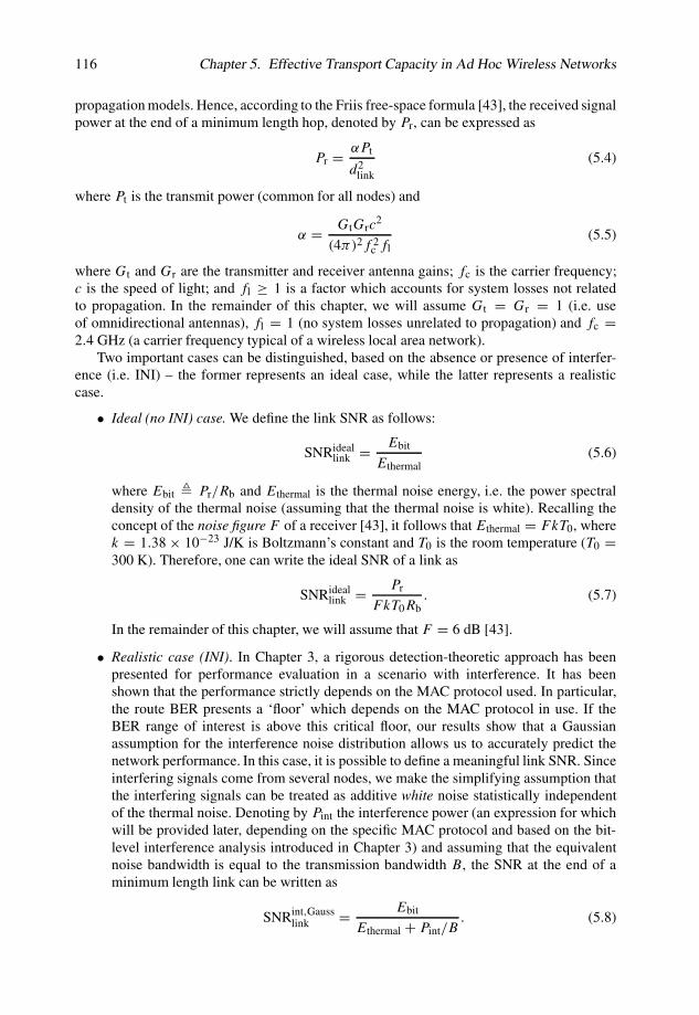
propagation models. Hence, according to the Friis free-space formula [43], the received signalpower at the end of a minimum length hop, denoted by Pr, can be expressed as

Pr = αPt

d2link

(5.4)

where Pt is the transmit power (common for all nodes) and

α = GtGrc2

(4π)2f 2c fl

(5.5)

where Gt and Gr are the transmitter and receiver antenna gains; fc is the carrier frequency;c is the speed of light; and fl ≥ 1 is a factor which accounts for system losses not relatedto propagation. In the remainder of this chapter, we will assume Gt = Gr = 1 (i.e. useof omnidirectional antennas), fl = 1 (no system losses unrelated to propagation) and fc =2.4 GHz (a carrier frequency typical of a wireless local area network).

Two important cases can be distinguished, based on the absence or presence of interfer-ence (i.e. INI) – the former represents an ideal case, while the latter represents a realisticcase.

• Ideal (no INI) case. We define the link SNR as follows:

SNRideallink = Ebit

Ethermal(5.6)

where Ebit � Pr/Rb and Ethermal is the thermal noise energy, i.e. the power spectraldensity of the thermal noise (assuming that the thermal noise is white). Recalling theconcept of the noise figure F of a receiver [43], it follows that Ethermal = FkT0, wherek = 1.38 × 10−23 J/K is Boltzmann’s constant and T0 is the room temperature (T0 =300 K). Therefore, one can write the ideal SNR of a link as

SNRideallink = Pr

FkT0Rb. (5.7)

In the remainder of this chapter, we will assume that F = 6 dB [43].

• Realistic case (INI). In Chapter 3, a rigorous detection-theoretic approach has beenpresented for performance evaluation in a scenario with interference. It has beenshown that the performance strictly depends on the MAC protocol used. In particular,the route BER presents a ‘floor’ which depends on the MAC protocol in use. If theBER range of interest is above this critical floor, our results show that a Gaussianassumption for the interference noise distribution allows us to accurately predict thenetwork performance. In this case, it is possible to define a meaningful link SNR. Sinceinterfering signals come from several nodes, we make the simplifying assumption thatthe interfering signals can be treated as additive white noise statistically independentof the thermal noise. Denoting by Pint the interference power (an expression for whichwill be provided later, depending on the specific MAC protocol and based on the bit-level interference analysis introduced in Chapter 3) and assuming that the equivalentnoise bandwidth is equal to the transmission bandwidth B, the SNR at the end of aminimum length link can be written as

SNRint,Gausslink = Ebit

Ethermal + Pint/B. (5.8)

5.4. Single-Route Effective Transport Capacity 117

In the case of binary phase shift keying (BPSK) signaling (which will be the modulationformat considered in the remainder of this chapter) B = Rb, so that one can write:

SNRint,Gausslink = Pr

FkT0Rb + Pint. (5.9)

We assume that there is full connectivity, in an average sense, when, at the end of a multi-hop route with an average number of hops, the BER is lower than a maximum prescribedvalue, denoted as BERmax

route. In other words, full connectivity is obtained if

BERroute ≤ BERmaxroute. (5.10)

Network connectivity has been analyzed in detail in Chapter 4 (on the basis of theresults presented in Chapters 2 and 3). In the following, we recall the concept of anaverage sustainable number of hops, which is a meaningful indicator (from a physical layerperspective) of connectivity.

5.3.3 Average Sustainable Number of HopsThe maximum sustainable number of hops, denoted as nmax

sh , corresponds to the maxi-mum number of hops such that the final BER at the end of a multi-hop route is equalto a maximum tolerable value BERmax

route. According to the results in Chapters 2 and 3, themaximum sustainable number of hops can be given as the following expressions, dependingon the presence or absence of interference:

nmaxsh =

⌊BERmax

route

BERlink

⌉without interference BERmax

route

max{

BERGausslink , BERMAC

link,floor

} with interference

(5.11)

where BERGausslink is the link BER under the Gaussian assumption for the interference noise and

BERMAClink,floor is the route BER floor associated with the MAC protocol used (the expressions

for this floor, in the cases with the RESGO and RESLIGO MAC protocols, can be found inChapter 3). The average sustainable number of hops can then be defined as

nsh � min{nmax

sh , nh}. (5.12)

For a more accurate description of the average sustainable number of hops, the reader isreferred to Chapters 2 and 3. In the following, we will use the concept of an averagesustainable number of hops to introduce the effective transport capacity.

5.4 Single-Route Effective Transport CapacityWe first observe that, based on the notion of an average sustainable number of hops, theaverage sustainable communication route length, denoted as droute, that a bit has to travelfrom the source to the destination can be written as

droute � nshdlink = nsh

√A

N= nsh

1√ρS

. (5.13)


At this point, if only a single route at a time were active in the wireless network, the effectivetransport capacity of the network would be given by the single-route effective transportcapacity, i.e. by the bit rate–distance product carried by this single route. More precisely,the single-route effective transport capacity can be defined as

Csreff � λLdroute (5.14)

where λL represents the average transmission rate at which the source node is transmitting.As explained in section 5.2, a fundamental underlying assumption in (5.14) is that only thesource node contributes to effective information transmission. Moreover, we are implicitlyassuming that the average transmission rate is equal to the average generation rate, asdiscussed in section 5.2. If only one route is active in the network, based on the modelconsidered and the assumptions outlined in section 5.2, it is possible to conclude that there isno INI.31 The single-route effective transport capacity can then be written as follows:

Csreff = λLnideal

sh1√ρS

. (5.15)

Since, in the ideal case, nidealsh does not depend on λ, it can be immediately concluded that the

maximum of the single-route effective transport capacity can be written as

Csreff,max = max

λ,Rb:λL≤RbCsr

eff = maxRb

Rb nidealsh

1√ρS

(5.16)

where the last equality is obtained by imposing λL = Rb. According to the consideredpacketized ad hoc wireless network communication model shown in Figure 5.1, the conditionλL = Rb corresponds to assuming that the source node is transmitting continuously(on average), i.e. its corresponding communication tube is completely filled.

In Figure 5.2, Csreff is shown as a function of the number of nodes, for two possible data-

rates. The values assumed for significant network parameters are also shown in the figure.From Figure 5.2, one can notice that the single-route effective transport capacity is a non-decreasing function32 of the number of nodes: it is strictly increasing for N < Nmin, whileit remains constant for N ≥ Nmin, where Nmin is given by (2.37) in Chapter 2, which isreported here for the sake of notational simplicity:

Nmin � FkT0SNRminlinkARb

αPt(5.17)

where, in the case of BPSK transmission and strong LOS,

SNRminlink = 1

2

{Q−1

[1 −

(1 − BERmax

route

)1/nh]}2

(5.18)

31Considering the case of a single route active at a time, a communication scenario without INI underlies theassumption that successive links of the same communication route do not interfere with each other. This is not truein a rigorous sense if there are simultaneous transmissions over successive links of the same multi-hop route, but itis a reasonable assumption in all considered communication scenarios.

32In Figure 5.2, one can observe a ‘saw-tooth’ behavior of the effective transport capacity, once the maximumhas been reached. This is due to the fact that for increasing values of N , the average sustainable number of hopsincreases: each saw tooth corresponds to an increase of 1 for the average number of sustainable hops.

5.4. Single-Route Effective Transport Capacity 119

0 1 103

2 103

3 103

4 103

5 103

N

0

1 107

2 107

3 107

4 107

5 107

6 107

Ceff

[b-m/s]

Rb= L=104 b/s

Rb= L=105 b/s

fc=2.4 GHz

Pt=10-7

W

F=6 dBA=10

6 m

2

BERroute

=10-3

Gt=Gr=fl=1

max

for Rb=104 b/s

Nmin

=122for Rb=10

5 b/s N

min=1290

sr

Figure 5.2 The single-route effective transport capacity versus the number of nodes.

where Q−1(·) represents the inverse function of Q(x) � 1√2π

∫ +∞x

e−y2/2 dy. This result

suggests that when the number of nodes N is above the threshold value Nmin, i.e. in the caseof full connectivity (on average), the effective transport capacity of a single active multi-hoproute depends on the data-rate and the area, but not on the number of nodes. Moreover, fromFigure 5.2 one can observe that for increasing data-rate, the number of nodes (or, equivalently,the node spatial density) needs to increase in order for the single-route effective transportcapacity to reach its maximum value.

In Figure 5.3, the single-route effective transport capacity is shown, as a function of thedata-rate, for various values of the traffic load. Observe the existence of a threshold valuefor the data-rate, given by Rmax

b in (2.31), such that, for a traffic load equal to this value,the effective transport capacity is maximized. For the sake of clarity, we report here theexpression of Rmax

b :

Rmaxb � αPtρS

FkT0SNRminlink

. (5.19)

This clearly distinguishes two situations: (i) if λL ≤ Rmaxb , then the effective transport

capacity is constant over the data-rate range between λL and Rmaxb , and monotonically

decreasing for Rb ≥ Rmaxb (in the limit, for λL = Rmax

b , the range over which the effectivetransport capacity is constant reduces to zero); (ii) if λL > Rmax

b , owing to the Rb ≥ λL

constraint, it follows that the effective transport capacity is always monotonically decreasing.In fact, if Rb > Rmax

b , the noise power increases dramatically (in the case of BPSK, the3 dB bandwidth is approximately equal to the data-rate), leading to a significant performancedegradation, which, in all cases, reduces the effective transport capacity. In this sense, the


0 1 105

2 105

Rb [b/s]

105

106

107

108

Ceff

sr

[b m/s]

L=2x104 b/s

L=5x104 b/s

L=8x104 b/s

fc=2.4 GHz

Pt=10

7 W

F=6 dB

S=10

3 m

2

BERroute

max=10

3

Rb

max=8x10

4 b/s

Gt=G

r=f

l=1

ConnectedNetwork

Disconnected

Network

Figure 5.3 Effective transport capacity versus data-rate, in the case of a single communica-tion route active at a time.

region corresponding to Rb ≥ Rmaxb is characterized by the absence of connectivity. Hence,

the only effective operative region for an ad hoc wireless network (without interference) isthe one with Rb < Rmax

b .

5.5 Aggregate Effective Transport CapacityAt this point, we propose a simple approach for the evaluation of the aggregate effectivetransport capacity33 of an ad hoc wireless network with disjoint multi-hop routes. First ofall, one needs to determine the number of different routes active in the network. Since theaverage number of hops in a multi-hop route is nh = �(

√N), there can be at most Nmax

ar �N/nh = �(

√N) disjoint active routes – the reason why disjoint routes are considered for

the evaluation of the effective transport capacity will be justified in more detail in section 5.8.A graphical example of this situation is shown in Figure 5.4, where each route is formed byfour hops – in the case of a circular network surface, nh = �√N/π� and Nmax

ar = �√Nπ�,so that the scenario in Figure 5.4 corresponds to a network with N = 50 nodes.

Obviously, in order for Nmaxar disjoint routes with nh hops to be simultaneously active, it

is necessary that all nodes in the network are simultaneously ‘engaged’. This is very unlikely,so that the effective number of active routes would probably be lower than Nmax

ar . On theother hand, it might happen that the maximum number of sustainable hops is lower than nh:in this case, one might argue that the number of disjoint routes could be larger than Nmax

ar .

33In the remainder of this chapter, the term effective transport capacity will refer to aggregate effective transportcapacity.

5.5. Aggregate Effective Transport Capacity 121

A

Communication Route(nh = �√N/π� = 4 hops)

Figure 5.4 Disjoint communication routes in an ad hoc wireless network with N = 50nodes.

However, in order to obtain a connectivity-based characterization of the effective transportcapacity, in the following we assume that there are Nmax

ar disjoint routes in the network,34 sothat: (i) if there is full connectivity, then each route is formed, on average, by nh = �√N/π�links (all the nodes in the network are used); (ii) if there is not full connectivity, then eachroute is formed by a maximum sustainable number of hops lower than nh. Extensions of theapproach proposed in this chapter to cases with a different number of active multi-hop routesare straightforward, by properly scaling the obtained results. Based on these considerations,the effective transport capacity, denoted by Ceff, can be defined as follows:

Ceff � Nmaxar Csr

eff = Nmaxar λLnshdlink. (5.20)

In the following, we consider the ideal (no INI) case and two realistic (INI) cases withthe RESGO and RESLIGO MAC protocols. The reader should recall that, in the remainderof this chapter, we assume a regular square grid topology (dlink = 1/

√ρS = √

A/N ) over acircular surface (Nmax

ar = �√Nπ�). In general, the proposed results are valid, on the order,for other regular topologies and surface shapes.

5.5.1 Ideal (no INI) Case

The effective transport capacity can be written as a function of the number of nodes (for afixed data-rate) or as a function of the data-rate (for a fixed number of nodes), respectively,

34It will be clear in the following that the basic principle of the RESLIGO MAC protocol is that of almost alwaysallowing only one route at a time to be active.


as follows:

Cidealeff = λLnideal

sh

√πA

=

λL

⌊√A N

⌉N ≥ Nmin

λL

⌊ln(1 − BERmax)

ln(1 − BERlink)

⌉ √πA N < Nmin

(5.21)

=

λL

⌊ln(1 − BERmax)

ln(1 − BERlink)

⌉ √πA Rb ≥ Rmax

b

λL⌊√

A N⌉

Rb < Rmaxb

(5.22)

where expressions for Nmin and Rmaxb are given by (5.17) and (5.19). As in the single-route

case, in this case as well, since nidealsh does not depend on λL, the overall maximum of the

effective transport capacity is simply obtained by substituting λL by Rb in (5.21) and (5.22),and then by maximizing with respect to Rb. As indicated in section 5.2, the assumptionλL = Rb corresponds to assuming that each multi-hop communication route is, on average,completely filled by packets. In the absence of INI, this is clearly desirable to maximize theexchange of information in the network.

The behavior of the effective transport capacity, as a function of the data-rate, is shown inFigure 5.5, for various values of the traffic load λL – note that for each value of the productλL the valid data-rate range corresponds to Rb ≥ λL. The values of the major networkparameters are indicated in the figure. The curves in Figure 5.5 are a shifted version ofthe curves in Figure 5.3 – the aggregate effective transport capacity is simply obtained bymultiplying the single-route effective transport capacity by the number Nmax

ar of active routes.The behavior of the effective transport capacity, as a function of the number of nodes,

is shown in Figure 5.6. As expected from (5.21), for N > Nmin, the effective transportcapacity is �(

√N), while for N < Nmin, it rapidly decreases to zero for decreasing values

of N (i.e. there is no connectivity). Hence, one can conclude that for values of N above thethreshold value, the effective transport capacity reaches the order bound proposed in [16] forthe transport capacity. For values of N below the threshold, however, the effective transportcapacity does not reach this information-theoretic upper bound, and this is due to loss ofconnectivity. In this sense, our results further refine and qualify the well-known results ofGupta and Kumar proposed in [16], by taking into account a prescribed maximum end-to-end BER at the end of a multi-hop route with an average number of hops. It is clearthat in [16] an information-theoretic approach is considered, where each transmission overa link is error-free, provided that the distance between the two nodes of the link is smallenough (under the non-interference protocol model) or the SNR at the receiving node is highenough (under the non-interference physical model). Hence, in [16] the authors considera hard distinction between the case where no errors are made and the case where notransmission is possible. In this book, we are proposing a different approach. In fact, inthe ideal case under examination we still assume that there is no INI (this is equivalent toconsidering an SNR above threshold for any communication link, for example using perfectlyorthogonal spreading codes or perfectly functioning directional antennas in different multi-hop routes), but we take into account the cumulative error effect due to thermal noise inmultiple hops. In this sense, we consider the degradation, in terms of BER, determined bychannel impairments.


0.0 5.0 104

1.0 105

1.5 105

Rb [b/s]

107

108

109

1010

Ceffideal

[b m/s]

L=2x104 b/s

L=5x104 b/s

L=8x104 b/s

fc=2.4 GHz

Pt=107 W

F=6 dB

A=106 m

2

BERroute

max =103

Rb

max=8x10

4 b/s

N=103

Gt=G

r=f

l=1

Figure 5.5 Effective transport capacity versus data-rate in the ideal (no INI) case.(Reproduced by permission of © 2003 IEEE.)

5.5.2 Realistic (INI) Case: RESGO MAC ProtocolThe RESGO MAC protocol has been introduced and described in Chapter 3. The basicprinciple of this MAC protocol is the provision that each node, after reserving a route,starts transmitting without sensing the channel. Moreover, no retransmission mechanism isconsidered in intermediate links – this minimizes the transmission delay. Extensions of thisMAC protocol to a network communication scenario where retransmission mechanisms areused in intermediate links are considered in Chapter 7. The reader is referred to Chapter 3 fora complete description of the RESGO MAC protocol.

The aggregate effective transport capacity35 can be written as

CRESGOeff = λLnRESGO

sh

√πA (5.23)

where nRESGOsh is the average sustainable number of hops in a realistic case with the RESGO

MAC protocol. Unlike the ideal case, where the average sustainable number of hops nidealsh

does not depend on λL, nRESGOsh does depend on λL – in fact, in Chapter 3 it is shown that the

average interference power with the RESGO MAC protocol, under the Gaussian assumption,depends on λL. Hence, the overall maximum of the effective transport capacity, given by

CRESGOeff,max = max

λL,Rb:λL≤RbCRESGO

eff (5.24)

35We emphasize that expression (5.23) is actually an upper bound on the effective transport capacity with theRESGO MAC protocol, in the sense that, based on the packet transmission rate, not all possible disjoint routes couldbe activated (there could be fewer than nh = �√Nπ� source nodes ready to transmit).


0 500 1000 1500 2000N

0.0

5.0 108

1.0 109

1.5 109

2.0 109

2.5 109

3.0 109

Ceff

[b-m/s]

L=Rb=104 b/s

L=Rb=5x104 b/s

L=Rb=105

b/s

fc=2.4 GHz

Pt=10-7

WF=6 dB

A=106 m

2

BERroute

max=10

-3

Gt=Gr=fl=1ideal

Figure 5.6 Aggregate effective transport capacity versus number of nodes in the ideal (noINI) case. (Reproduced by permission of © 2003 IEEE.)

cannot be obtained by replacing λL with Rb and then maximizing with respect to Rb. In otherwords, if packets flow continuously inside each route (i.e. λL = Rb), on average, the INI isintolerable and the BER performance becomes unacceptable.

In Figure 5.7, the effective transport capacity is shown, as a function of the data-rate Rb,for various values of the traffic load λL. In particular, in (a) the transmit power is set toPt = 10−5 W, whereas in (b) Pt = 10−4 W.

(a) In the scenario with Pt = 10−5 W, shown in Figure 5.7 (a), one can observe that forincreasing values of the per-node traffic load λL, the maximum value (with respect tothe data-rate) of the effective transport capacity increases. In particular, for each valueof the traffic load, there is a data-rate range over which the effective transport capacity isconstant and maximum (there is connectivity), and outside which the effective transportcapacity rapidly drops to zero (connectivity is lost). Note that for λL = 400 b/s,the data-rate range where connectivity is guaranteed almost shrinks to zero. It canbe shown that for higher values of the traffic load the maximum effective transportcapacity decreases, and connectivity can never be reached.

(b) In Figure 5.7 (b), the behavior of the effective transport capacity is shown for Pt =10−4 W (all the other network parameters are the same as in Figure 5.7 (a)). Fromthe obtained results, one can deduce that an increase of the transmit power has thebeneficial effect of increasing network connectivity. In fact, comparing each curve,for a given value of λL, with the equivalent one in Figure 5.7 (a), one can observethat the data-rate range over which the effective transport capacity is constant andmaximum (i.e. over which the network is connected) is wider than in the scenario with


0.0 5.0 106

1.0 107

1.5 107

Rb [b/s]

103

104

105

106

107

108

Ceff

[b-m/s]

L=10 b/sL=100 b/sL=130 b/sL=200 b/sL=400 b/s

fc=2.4 GHz

Pt=10-5

WF=6 dB

A=106 m

2

BERroute

max=10

-3

N=103

Gt=Gr=fl=1ConnectedNetwork

Network

Disconnected

RESGO

(a)

0.0 5.0 107

1.0 108

1.5 108

2.0 108

Rb [b/s]

103

104

105

106

107

108

Ceff

[b-m/s]

L=10 b/sL=100 b/sL=130 b/sL=200 b/sL=400 b/sL=2 kb/s

fc=2.4 GHz

Pt=10-4

WF=6 dB

A=106 m

2

BERroute

max =10-3

N=103

Gt=Gr=fl=1

ConnectedNetwork

NetworkDisconnected

RESGO

(b)

Figure 5.7 Effective transport capacity versus data-rate in a realistic (INI) scenario with theRESGO MAC protocol, for (a) Pt = 10−5 W and (b) Pt = 10−4 W. Various values of thetraffic load λL are considered. The major network parameters are indicated in the figure.

lower transmit power. Moreover, using a higher transmit power allows one to supportconnectivity for larger traffic loads (e.g. λL = 2 kb/s). Note, however, that for valuesof λL such that the network is connected for both high and low transmit power, themaximum effective transport capacity is the same in both cases.


101

102

103

λL [b/s]

105

106

Ceff

[b-m/s]

Rb=500 kb/s, Pt=5x10-7

W

Rb=500 kb/s, Pt>=10-6

W

Rb=1 Mb/s, Pt=10-6

W

Rb=1 Mb/s, Pt>=5x10-6

W

fc=2.4 GHzF=6 dB

ρS=10-3

m-2

BERroute

=10-3

Gt=Gr=fl=1

max

RESGO

Figure 5.8 Effective transport capacity versus traffic load λL, for various values of thetransmit power Pt and data-rate Rb, in a realistic scenario (with INI) with the RESGO MACprotocol.

Numerical results show that the overall maximum of the effective transport capacity doesnot increase without limit by increasing the transmit power. This is shown in Figure 5.8,where the effective transport capacity is evaluated, as a function of the traffic load λL, forvarious values of the transmit power Pt and data-rate Rb. In particular, our results show thatfor each data-rate, increasing the transmit power beyond a critical value does not change theeffective transport capacity: this critical transmit power is 10−6 W for Rb = 500 kb/s (solidline in Figure 5.8) and 5 × 10−6 W for Rb = 1 Mb/s (dashed line in Figure 5.8). Note alsothat there is a characteristic behavior: in fact, the effective transport capacity increases linearlywith the traffic load λL up to a point beyond which it saturates and remains constant. Moreprecisely, one can observe a ‘saw-tooth’ behavior. This is due to the loss of connectivity: eachoscillation corresponds to a reduction by 1 of the average sustainable number of hops. Thisobservation is clarified in Figure 5.9, where the average sustainable number of hops is shownas a function of the traffic load λL. Comparing Figure 5.9 with Figure 5.8, one can concludethat the effective transport capacity saturates once connectivity is lost, i.e. the average numberof sustainable hops is lower than nh = �√N/π� = 18. Finally, one can observe that if thetransmit power is too low (e.g. Pt = 5 × 10−7 W for Rb = 500 kb/s and is Pt = 10−6 Wfor Rb = 1 Mb/s) the average sustainable number of hops never reaches nh (i.e. there is noconnectivity) and the effective transport capacity is lower than in the case where connectivityis guaranteed. The behavior of the effective transport capacity can be characterized as follows.

• For large data-rate, the thermal noise power is large. However, for low traffic loads theinterference is small. Since in Chapter 3 it has been shown that the route BER floor isproportional to the ratio λL/Rb, it follows that the route BER floor is very low and the


101

102

103

λL [b/s]

0

2

4

6

8

10

12

14

16

18

20

nsh

Rb=500 kb/s, Pt=5x10-7

W

Rb=500 kb/s, Pt>=10-6

W

Rb=1 Mb/s, Pt=10-6

W

Rb=1 Mb/s, Pt>=5x10-6

W

fc=2.4 GHzF=6 dB

A=106 m

2

BERroute

=10-3

Gt=Gr=fl=1

max

N=1000

Figure 5.9 Average sustainable number of hops versus traffic load λL, for various values ofthe transmit power Pt and the data-rate Rb, in a realistic scenario (with INI) with the RESGOMAC protocol.

desired route BER QoS (i.e. BERmaxroute) can be guaranteed, provided that the transmit

power is sufficiently high. For increasing traffic load, the interference level increasesand the route BER floor becomes higher. At some point, the route BER QoS cannot beguaranteed, regardless of the transmit power, and connectivity is lost.

• For low data-rate, even though the thermal noise power may be negligible, the routeBER floor is for relatively high also relatively low traffic loads. In fact, the maximumeffective transport capacity which can be achieved before connectivity breaks down islower than the scenario with a high data-rate.

In all cases (both for high and low data-rate), at some point the effective transport capacitydrops to zero. This corresponds to a scenario where the traffic load (and, consequently, theinterference) is so high that even single-link communications cannot be supported.

Finally, in Figure 5.10, the effective transport capacity is shown as a function of thenumber of nodes N , for two possible values of λL (10 and 100 b/s, respectively) and twopossible values of the transmit power Pt (0.1 and 0.01 mW, respectively). As one can seefrom the figure, when λL = 100 b/s the effective transport capacity curves reach a muchhigher value (around 2.3 × 106 b m/s) than in the case with λL = 10 b/s. However, whilein the former case the effective transport capacity saturates at the maximum, i.e. it remainsconstant for increasing numbers of nodes, in the latter case the effective transport capacitygrows as

√N (this is not clearly visible in the scale of Figure 5.10, but it will be clear from

Figure 5.11). Note also that if Pt = 0.01 mW, for both considered values of λL the effective


0 200 400 600 800 1000N

0.0

5.0×105

1.0×106

1.5×106

2.0×106

2.5×106

3.0×106

Ceff

RESGO

[b−m/s]

Pt=0.1 mW

Pt=0.01 mW

fc=2.4 GHz

Rb=10

6 b/s

F=6 dBA=10

6 m

2

BERroute

=10−3

Gc=G

r=f

l=1

λL=100 b/s

max

λL=10 b/s

Figure 5.10 Effective transport capacity versus the number of nodes N in a realistic (INI)scenario with the RESGO MAC protocol. Various values of the transmit power and trafficload are considered.

transport capacity is zero for low values of N . This is due to the absence of connectivity,as can be understood from the results in Figure 5.11, where the average sustainable numberof hops is shown, as a function of the number of nodes, in the four scenarios considered inFigure 5.10. From the results in Figure 5.11, it is clear that for N ≤ 100, if Pt = 0.01 mWthen the average sustainable number of hops is lower than nh, i.e. there is no connectivity,and the same behavior is obtained for both λL = 10 b/s and λL = 100 b/s. On the otherhand, for N ≥ 570 the average sustainable number of hops in the scenario with high trafficload (λL = 100 b/s) saturates to 13 hops, whereas in the scenario with low traffic load(λL = 10 b/s) the average number of hops increases as

√N . The saturation observed in the

presence of high traffic load is due to the fact that the limiting BER floor with the RESGOMAC protocol increases proportionally to the traffic load λL (see Chapter 3 for more details):at some point, this floor becomes so high that a number of hops larger than 13 cannot besupported with the desired QoS constraint in terms of maximum tolerable BER at the end ofa multi-hop route.

5.5.3 Realistic (INI) Case: RESLIGO MAC ProtocolAs seen in Chapter 3, the RESLIGO MAC protocol is characterized by the fact that a node,after reserving a multi-hop route to its destination, senses the channel before activating theroute: if no transmission is going on, then the source node starts transmitting, i.e. it activatesthe route (the packets ‘go’). The evaluation of the effective transport capacity of an ad hocwireless network when using this MAC protocol can be carried out along the same lines as forthe previous MAC protocol. However, a fundamental observation has to be made. In fact, inboth the ideal case and in a realistic case with the RESGO MAC protocol, we have assumed


0 200 400 600 800 1000N

0

4

8

12

16

20

nsh

nh=Θ(Ν1/2)λL=10 b/s

λL=100 b/s

Pt=0.1 mW

Pt=0.01 mW

Figure 5.11 Average sustainable number of hops versus the number of nodes N in a realistic(INI) scenario with the RESGO MAC protocol. The four scenarios considered in Figure 5.10are examined.

that Nmaxar multi-hop routes can be active at the same time. This assumption is no longer valid

in the case with the RESLIGO MAC protocol. As will be shown in the following, providedthat the receiver sensitivity is ideal, if the traffic load is not too heavy, use of the RESLIGOMAC protocol leads, almost always, to the activation of only one route at a time, thus reducingthe interference dramatically. If the traffic load is very high, however, it might happen thatsource nodes far from each other activate their routes simultaneously. In this case, since theroutes are far from each other, the INI is limited and the effective transport capacity canbe even higher than that in a scenario where only one route is active. In other words, thiscorresponds to exploiting spatial reuse to increase the transfer of information in the network.If the receiver sensitivity is not ideal, then spatial reuse becomes automatic if the RESLIGOMAC protocol is used. The subsequent analysis can be extended to the latter case followingthe approach proposed in [132].

In order to derive an expression for the effective transport capacity, the number of routeswhich can simultaneously be activated has to be evaluated. Assume that at a given time, nocommunication route is active. At this point, there might be more than one source node whichsimultaneously decide to access the shared medium to activate their own (already created)communication route. Referring to the considered tiered structure in Figure 3.3, where thenodes are at the vertices of a square grid, we assume that the central node is a source nodewhich is activating a corresponding communication route. Pessimistically, assume that allthe other nodes in the network might be potential source nodes which want to activate theirown communication routes as well.36 Given that the propagation time for any transmission is

36We observe that since each route needs relay nodes, such relay nodes cannot be other source nodes. However,since we are concerned with an upper bound and for the sake of a simple mathematical derivation, we assume(pessimistically) that all the remaining nodes, except for the central one, are potential interfering sources.


much smaller than the packet duration (of the order of L/Rb), it is possible to show that thenumber NRESLIGO

rn of nodes, which can activate a communication route interfering with theone activated by the central node, can be upper bounded as follows:37

NRESLIGOrn ≤

⌊imax∑i=1

[4(1 − e−2λiτlink) + 4(1 − e−2

√2λiτlink)

+ 8i−1∑j=1

(1 − e−2√

2λiτlink)

]⌉. (5.25)

Recalling that, on average, there cannot be more than Nmaxar active multi-hop routes at a time,

the number NRESLIGOar of active routes38 is

NRESLIGOar � max

{1, min

{NRESLIGO

rn , Nmaxar

}}. (5.26)

Given this definition, in the case of a circular network surface and a regular square gridtopology, the effective transport capacity with the RESLIGO MAC protocol can be written as

CRESLIGOeff � NRESLIGO

ar λLnRESLIGOsh

√A

N(5.27)

where nRESLIGOsh is the average number of sustainable hops. It is possible to show that if the

network size and the average packet generation rate λ are not extremely large, NRESLIGOar = 1

and the interference is basically reduced to zero, so that the effective transport capacity inthe case of the RESLIGO MAC protocol basically coincides with the single-route effectivetransport capacity. In other words,

CRESLIGOeff � Csr

eff. (5.28)

In Figure 5.12, the effective transport capacity in the case with the RESLIGO MACprotocol is shown as a function of the data-rate, for various values of the average packettransmission rate39 λ. Observe that for all considered values of λ, for Rb ≥ 8 × 106 b/sthe effective transport capacity drops to zero, i.e. connectivity is lost. For comparison, inFigure 5.12 the behavior of the effective transport capacity in a scenario with the RESGOMAC protocol and λ = 0.2 pck/s (λL = 200 b/s) is shown. Comparing this curve withthe equivalent curve for the RESLIGO MAC protocol for the same traffic load, it can beconcluded that, for sufficiently high data-rate, the maximum value of the effective transportcapacity in the first case (with RESGO) far exceeds the maximum value in the second case(with RESLIGO). Note, however, that for low data-rate, the effective transport capacity withthe RESGO MAC protocol drops rapidly to zero, i.e. connectivity is lost. We directly comparethe two considered MAC protocols in the next section.

37Since the derivation of this upper bound is based on geometric considerations along the lines of the approachconsidered in Chapter 3, we omit the details of the derivation in this chapter.

38The definition of the number of active routes takes into account the fact that in some cases NRESLIGOrn could be

zero, but we are assuming that at least one communication route is active.39The reader should observe that in the case with the RESGO MAC protocol, the performance is evaluated in

terms of λL. However, in the case with the RESLIGO MAC protocol, in Chapter 3 it is shown that the route BERfloor depends on λ, but not on the packet length L. Therefore, in order to analyze the performance with the RESLIGOMAC protocol, one has to indicate separately both λ and L.

5.6. Comparison of the RESGO and RESLIGO MAC Protocols 131

0.0 4.0 106

8.0 106

1.2 107

1.6 107

2.0 107

Rb [b/s]

104

105

106

107

108

Ceff

[b-m/s]

=0.2 pck/s - RESGO=0.2 pck/s - RESLIGO=10 pck/s - RESLIGO=40 pck/s - RESLIGO=80 pck/s - RESLIGO=300 pck/s - RESLIGO

fc=2.4 GHz

Pt=10-5

WF=6 dB

A=106 m

2

BERroute

=10-3

N=103

Gt=Gr=fl=1

max

L=103

RESLIGO

Figure 5.12 Effective transport capacity versus data-rate in a realistic (INI) case with theRESLIGO MAC protocol. Various values of the traffic load λL are considered.

5.6 Comparison of the RESGO and RESLIGO MACProtocols

After analyzing the performance, in terms of the effective transport capacity, for eachconsidered MAC protocol individually, a direct comparison can provide further insight.In particular, the performance of the proposed MAC protocols is compared based on threeuseful quantities: (i) the maximum achievable effective transport capacity40 (suitably fixingthe transmission data-rate) for each value of λ; (ii) the minimum data-rate Rmin

b necessary tomaximize the effective transport capacity; and (iii) the data-rate range (starting from Rmin

b )over which the effective transport capacity is maximized.

In Figure 5.13, the behavior of the maximum effective transport capacity, as a functionof λ (for L = 1000 b/pck), is shown – in other words, each point of the curve indicatesthe maximum possible effective transport capacity, over all possible data-rates, for thecorresponding value of λ. Considering the ideal (no INI) case, one can see that the maximumachievable effective transport capacity is a linear function of λ up to a maximizing valueλideal,max (λideal,max � 800 pck/s for Pt = 1 µW and λideal,max � 80 pck/s for Pt = 0.1 µW)– the maximizing value in the case with Pt = 0.1 µW was expected from Figure 5.5.For traffic loads larger than λideal,max, since Rb ≥ λL, the thermal noise power is solarge that the effective transport capacity rapidly drops to zero. Considering the RESGOMAC protocol, the maximum effective transport capacity coincides with that obtained in the

40Note that this quantity should not be confused with the transport capacity, interpreted as the overall maximumover all possible values of data-rate and traffic load [16].


10-3

10-2

10-1

100

101

102

103

λ [pck/s]

102

103

104

105

106

107

108

109

1010

1011

Ceff,max

[b-m/s]

Ideal, Pt=1 µW

RESGO, Pt>=1 µW

RESLIGO, Pt=1 µW

Ideal, Pt=0.1 µW

RESGO, Pt=0.1 µW

RESLIGO, Pt=0.1 µW

fc=2.4 GHz

max

F=6 dB

A=106 m

2

BERroute

=10-3

N=103

L=103 b/pck

Gt=Gr=fl=1

RESGO

RESLIGO

Ideal

Figure 5.13 Maximum effective transport capacity versus λ. The performance, in a realistic(INI) scenario, with RESGO and RESLIGO MAC protocols is compared to that in an ideal(no INI) scenario. Two possible values for the transmit power are considered.

ideal case for low traffic loads. At some point, the effective transport capacity curve stopsincreasing linearly with λ and flattens. This corresponds to the loss of full connectivity, i.e.the maximum sustainable number of hops is lower than the average number. For larger valuesof λ, the effective transport capacity drops to zero. The following theorem characterizes theperformance, in terms of the effective transport capacity, which can be obtained when usingthe RESGO MAC protocol.

Theorem 1. In the considered ad hoc wireless network communication scenario with strongLOS, the effective transport capacity of a realistic (INI) case with the RESGO MAC protocolcoincides with that of the ideal (no INI) case if the following three conditions are satisfied:

ξRESGOcaLOSnhλL

Rb< BERmax

route (5.29)

λL

ρSPt= ξ2α

4kT0F A(N)(SNRmin

link

)2 , ξ ≤ 1

3(5.30)

Rb = αρSPt

kT0FSNRminlink

(5.31)

where ξ is a power ratio, ξRESGO = 3 and caLOS = 0.25 (see Chapter 3), BERmaxroute is the

maximum tolerable BER at the end of a multi-hop route and

SNRminlink = 1

2

{Q−1

[1 − (

1 − BERmaxroute

)1/nh]}2

.

5.6. Comparison of the RESGO and RESLIGO MAC Protocols 133

Proof. See Appendix B.

Note that for decreasing values of Pt, the maximum value of λ for which the effectivetransport capacity coincides with that in the ideal case reduces. Moreover, it can be verifiedthat for Pt ≥ 1 µW the effective transport capacity with the RESGO MAC protocol remainsthe same.

From Figure 5.13, one can observe that the overall maximum of the effective transportcapacity with the RESGO MAC protocol is about four orders of magnitude lower than that inthe ideal case. When considering the RESLIGO MAC protocol, for low values of the trafficload, the achievable effective transport capacity is almost two orders of magnitude lower thanin the ideal case and in the case with the RESGO MAC protocol. However, for increasingtraffic loads, while the effective transport capacity with the RESGO MAC protocol saturatesand then drops to zero, the effective transport capacity with the RESLIGO MAC protocolkeeps on increasing. In fact, as expected, the maximum achievable effective transport capacitywith the latter MAC protocol is almost a scaled version (the scaling factor corresponds to thenumber of active routes Nmax

ar ) of the effective transport capacity in the ideal case. Note thatwe just wrote ‘almost a scaled version’, since one can observe from Figure 5.13 that this isexact when Pt = 0.1 µW; however, when Pt = 1 µW, for values of λ slightly lower thanthat corresponding to the maximum in the ideal case, the effective transport capacity withthe RESLIGO MAC protocol saturates before dropping to zero. It can be shown that thiscorresponds to a loss of connectivity which is due to the fact that the route BER floor with theRESLIGO MAC protocol (proportional to λ) becomes higher than BERmax

route (see Chapter 3for more details).

In Figure 5.14, the minimum data-rate necessary to maximize the effective transportcapacity is shown as a function of λ. In particular, for each case we have explicitly indicatedthe maximum value of λ corresponding to which connectivity breaks down. One can observethat for increasing values of the transmit power, the minimum required data-rate increases.In the case with the RESGO MAC protocol the minimum required data-rate is significantlyhigher than that in the ideal case, and this is due to the fact that the data-rate needs to beincreased in order to reduce the INI (by reducing the duration of a packet transmission).On the other hand, in the ideal/RESLIGO case, for a low transmit power (Pt = 0.1 µW)the maximum value of λ is the same, whereas for a higher transmit power (Pt = 1 µW)connectivity with the RESLIGO MAC protocol breaks down earlier than in the ideal case(as observed in Figure 5.13).

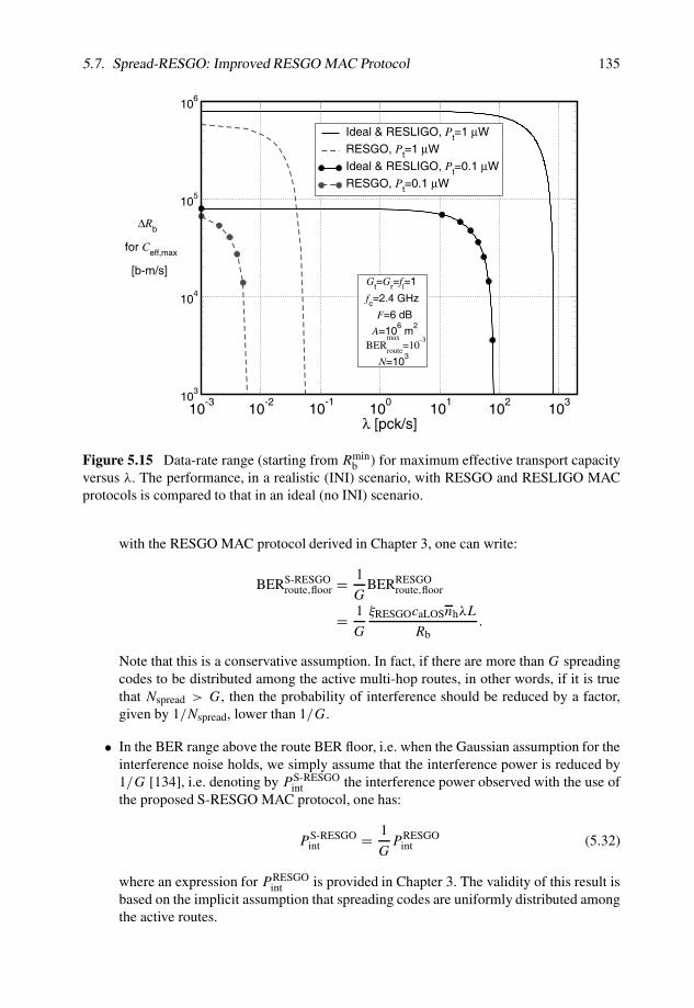
Finally, in Figure 5.15 the data-rate range, over which the effective transport capacity ismaximized, is shown as a function of λ. As in the figure relative to the minimum data-rateRmin

b , in this case as well the curves corresponding to the ideal and RESLIGO MAC protocol-based network communication scenarios coincide, whereas the curve corresponding to thecase with the RESGO MAC protocol is lower and reduces significantly (approaching zero)for lower values of λ. In other words, the range of data-rates over which the effective transportcapacity is maximized, reduces when considering the RESGO MAC protocol, implying thatthe transmission data-rate has to be carefully selected depending on the network traffic load.Moreover, one can observe that in each case (either ideal/RESLIGO or RESGO), increasingthe transmit power has a beneficial effect, in the sense that the data-range over which theeffective transport capacity is maximized and there is full connectivity widens.


10-3

10-2

10-1

100

101

102

103

λ [pck/s]

100

101

102

103

104

105

106

107

Rb

for Ceff,max

[b-m/s]

Ideal & RESLIGORESGO

fc=2.4 GHz

F=6 dB

A=106 m

2

BERroute

=10-3

N=103

Gt=Gr=fl=1

max

λmax for Pt=0.1 µW

λmax for Pt>=1 µW

λmax for Pt=0.1 µW

λmax for Pt=1 µW

λmax for Pt=1 µW

min

Ideal

RESLIGO

Ideal & RESLIGO

Figure 5.14 Minimum data-rate Rminb to achieve the maximum effective transport capacity

versus λ. The performance, in a realistic (INI) scenario, with RESGO and RESLIGO MACprotocols is compared to that in an ideal (no INI) scenario.

5.7 Spread-RESGO: Improved RESGO MAC Protocolwith Per-route Spreading Codes

In section 5.6, it was shown that the RESGO MAC protocol yields no performance loss,with respect to the ideal case, for very low values of the traffic load. Obviously, it wouldbe extremely beneficial to modify this MAC protocol in such a way that there is a limitedperformance loss, with respect to the ideal case, also for larger values of the averagetransmission rate. A simple approach for achieving this is to assign a spreading code to eachcommunication route. We will refer to this version of the RESGO MAC protocol as a spread(S)-RESGO MAC protocol. Note that this is similar to what was proposed in [67] for randomaccess wireless networks where the Aloha MAC protocol is used. Use of spreading codes fordistributed spread-spectrum packet radio networks is also considered in [65]. In the following,we present a simple-minded analysis of the benefits which the use of spreading codes couldbring about. The proposed approach can be refined by designing per-route spreading codesspecifically tailored for this scenario [133].

Let us consider a family of Nspread spreading codes with a spreading factor G. We nowpropose a reasonable (yet intuitive) extension of the analytical approach considered inChapter 3 for a performance analysis with the RESGO MAC protocol, distinguishing betweenthe route BER floor and the BER region above it.

• Regarding the route BER floor, we simply assume that it is G times lower than in thecase with the RESGO MAC protocol. Recalling the expression for the floor route BER

5.7. Spread-RESGO: Improved RESGO MAC Protocol 135

10-3

10-2

10-1

100

101

102

103

λ [pck/s]

103

104

105

106

∆Rb

for Ceff,max

[b-m/s]

Ideal & RESLIGO, Pt=1 µW

RESGO, Pt=1 µW

Ideal & RESLIGO, Pt=0.1 µW

RESGO, Pt=0.1 µW

fc=2.4 GHz

F=6 dB

A=106 m

2

BERroute

=10-3

N=103

Gt=Gr=fl=1

max

Figure 5.15 Data-rate range (starting from Rminb ) for maximum effective transport capacity

versus λ. The performance, in a realistic (INI) scenario, with RESGO and RESLIGO MACprotocols is compared to that in an ideal (no INI) scenario.

with the RESGO MAC protocol derived in Chapter 3, one can write:

BERS-RESGOroute,floor = 1

GBERRESGO

route,floor

= 1

G

ξRESGOcaLOSnhλL

Rb.

Note that this is a conservative assumption. In fact, if there are more than G spreadingcodes to be distributed among the active multi-hop routes, in other words, if it is truethat Nspread > G, then the probability of interference should be reduced by a factor,given by 1/Nspread, lower than 1/G.

• In the BER range above the route BER floor, i.e. when the Gaussian assumption for theinterference noise holds, we simply assume that the interference power is reduced by1/G [134], i.e. denoting by P S-RESGO

int the interference power observed with the use ofthe proposed S-RESGO MAC protocol, one has:

P S-RESGOint = 1

GP RESGO

int (5.32)

where an expression for P RESGOint is provided in Chapter 3. The validity of this result is

based on the implicit assumption that spreading codes are uniformly distributed amongthe active routes.


In Figure 5.16, the effective transport capacity with the S-RESGO MAC protocol isshown, as a function of the number of nodes N , for various values of the spreading factorG, and for (a) Pt = 0.1 µW and (b) Pt = 0.1 mW. For comparison, the effective transportcapacity curves in a realistic case with the RESGO MAC protocol (G = 1) and in the idealcase (G = ∞) are also shown.

• For a very low transmit power (Pt = 0.1 µW), one can see from Figure 5.16 (a) that inthe ideal case full connectivity is reached around N � 15 000 – in fact, for lower valuesof N the effective transport capacity does not have a �(

√N)-like behavior, but, rather,

falls to zero very rapidly. If the RESGO MAC protocol is used, connectivity is neverreached and the effective transport capacity is significantly lower than in the ideal case.Using the S-RESGO MAC protocol, for increasing values of G the effective transportcapacity reaches that in the ideal case, up to a critical number of nodes beyond which itremains constant (the interference becomes too high). Note that only for G = 6 is fullconnectivity reached, between N � 15 000 and N � 20 000.

• For higher values of the transmit power (Pt = 0.1 mW in Figure 5.16 (b)), the networkis always connected in the ideal case. In this case, if the RESGO MAC protocol is used,full connectivity is guaranteed up to N � 500, at which point the effective transportcapacity saturates and remains constant. In this case, use of S-RESGO with increasingvalues for the spreading factor G allows one to maintain connectivity up to larger valuesof the number of nodes N , i.e. higher node spatial densities (since the network area isfixed).

In Figure 5.17, the maximum (with respect to Rb) effective transport capacity with theS-RESGO MAC protocol is shown as a function of λ, for various values of the spreadingfactor G. As one can see, for larger values of the spreading factor the performance obtainedwith the S-RESGO MAC protocol coincides with that in the ideal case for a larger rangeof values of λ. Note, however, that the improvement is not dramatic. While we have scaledthe route BER floor by 1/G, in a realistic situation it would probably be reasonable to scaleit by a smaller factor (1/Nspread < 1/G), therefore improving the performance with theS-RESGO MAC protocol. As considered before, the maximum effective transport capacity,shown in Figure 5.17, is obtained by optimizing the transmission data-rate. As in a networkcommunication scenario with the RESGO MAC protocol, for a given value of λ (and L), themaximum value of the effective transport capacity is obtained when the transmission data-rate belongs to a specific range of length Rb starting at Rmin

b . The behaviors of Rminb and

Rb are shown in Figures 5.18 and 5.19, respectively. Observe that, for increasing values ofthe spreading factor G, Rmin

b decreases and Rb increases. In other words, there is a wideroperating region, for the ad hoc wireless network, where the effective transport capacity ismaximized.

At this point, one may wonder if the use of spreading codes in ad hoc wireless networksis practical or reasonable. In particular, the performance results shown in this section assumethat there is a ‘uniform’ distribution of the spreading codes among the possible activeroutes. This would be certainly possible, if there was a central authority. Unfortunately, thisis not the case in an ad hoc wireless network with a flat architecture. Nonetheless, it isrealistic to assume that in each route the destination node, at the moment of route creation,chooses randomly a spreading code (to be used in the route) among the Nspread possibleones. Recalling the maximum number Nmax

ar of average-length routes, one can identify twoimportant cases.

5.7. Spread-RESGO: Improved RESGO MAC Protocol 137

0 500 1000 1500 2000 2500 3000 3500 4000N

0

1 106

2 106

3 106

4 106

5 106

6 106

7 106

Ceff

[b-m/s]

IdealRESGOS-RESGO (G=2)S-RESGO (G=4)

fc=2.4 GHz

Rb=106 b/s

F=6 dBA=10

6 m

2

BERroute

max=10

-3

Pt=10-4

W

Gt=Gr=fl=1

L=100 b/s

(a)

5000 10000 15000 20000 25000 30000N

0.0

4.0 106

8.0 106

1.2 107

1.6 107

2.0 107

Ceff

[b-m/s]

IdealRESGOS-RESGO (G=2)S-RESGO (G=4)S-RESGO (G=6)

fc=2.4 GHz

Rb=106 b/s

F=6 dBA=10

6 m

2

BERroute

=10-3

Pt=10-7

W

Gt=Gr=fl=1

max

L=100 b/s

(b)

Figure 5.16 Effective transport capacity versus the number of nodes N , in a realistic (INI)scenario, with the RESGO MAC protocol (G = 1) and the S-RESGO MAC protocol(for various values of the spreading factor G > 1), in the cases with (a) Pt = 0.1 µWand (b) Pt = 0.1 mW. For comparison, the effective transport capacity in the ideal (no INI)case is also shown.


10-3

10-2

10-1

100

101

102

λ [pck/s]

102

103

104

105

106

107

108

109

1010

1011

Ceff,max

[b-m/s]


fc=2.4 GHz

Pt=10-7

WF=6 dB

A=106 m

2

BERroute

=10-3

N=103

Gt=Gr=fl=1

max

Figure 5.17 Maximum effective transport capacity versus λ, in a realistic (INI) scenario withthe RESGO and S-RESGO MAC protocols (for various values of the spreading factor G).For comparison, the effective transport capacity in the ideal (no INI) case is also shown.

• If Nspread ≥ Nmaxar , then it is possible that each route is assigned a different spreading

code. More precisely, the probability of this event, denoted as Pdiff-spread, can be writtenas follows:

Pdiff-spread =Nmax

ar −1∏i=0

Nspread − i

Nspread. (5.33)

If Nspread � Nmaxar , then Pdiff-spread � 1.

• If Nspread < Nmaxar , then Pdiff-spread = 0. However, it is reasonable to assume (due to

random assignment of the codes) that groups of approximately Nmaxar /Nspread routes

will select the same spreading code.

More research is needed to investigate the improvement brought by the use of spreadingcodes. Finally, we note that although the approach proposed in this section to reduce theinterference is based on the possible use of spreading codes, the same conclusions hold,qualitatively, as well if different multi-hop routes are separated in frequency, i.e. differentfrequency bands are assigned to different multi-hop routes.

5.8 DiscussionThe obtained results raise interesting questions, and suggest possible new research directions.We now comment on some aspects which appear to be important.

5.8. Discussion 139

10-3

10-2

10-1

100

101

102

λ [pck/s]

100

101

102

103

104

105

106

Rb

for Ceff,max

[b-m/s]


fc=2.4 GHz

Pt=10-7

W

F=6 dBA=10

6 m

2

BERroute

=10-3

N=103

Gt=Gr=fl=1

max

min

Figure 5.18 Minimum data-rate Rminb to achieve maximum effective transport capacity

versus λ, in a realistic (INI) scenario with the RESGO and S-RESGO MAC protocols(for various values of the spreading factor G). For comparison, the minimum data-rate inthe ideal (no INI) case is also shown.

10-3

10-2

10-1

100

101

102

λ [pck/s]

103

104

105

∆Rb

for Ceff,max

[b-m/s]


fc=2.4 GHz

Pt=10-7

WF=6 dB

A=106 m

2

BERroute

=10-3

N=103

Gt=Gr=fl=1

max

Figure 5.19 Data-rate range (starting from Rminb ) for the maximum effective transport

capacity versus λ, in a realistic (INI) scenario with the RESGO and S-RESGO protocols(for various values of the spreading factor G). For comparison, the data-rate range in theideal (no INI) case is also shown.


Cbeforeeff = 3Rbdroute

D3

D2

D1 D1

D2

D3

D4

S4

S1

S2

S3

S1

S2

S3

Caftereff = 4

Rb

2droute

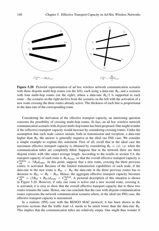
Figure 5.20 Pictorial representation of ad hoc wireless network communication scenariowith three disjoint multi-hop routes (on the left), each using a data-rate Rb, and a scenariowith four multi-hop routes (on the right), where a data-rate Rb/2 is supported in eachroute – the scenario on the right derives from the scenario on the left with the activation of anew route crossing the three routes already active. The thickness of each line is proportionalto the data-rate of the corresponding route.

Considering the derivation of the effective transport capacity, an interesting questionconcerns the possibility of crossing multi-hop routes. In fact, an ad hoc wireless networkcommunication scenario with disjoint multi-hop routes has been proposed. One might wonderif the (effective) transport capacity would increase by considering crossing routes. Under theassumption that each node cannot sustain, both in transmission and reception, a data-ratehigher than Rb, the answer is generally negative in the ideal (no INI) case. We considera simple example to explain this statement. First of all, recall that in the ideal case themaximum effective transport capacity is obtained by considering Rb = λL, i.e. when thecommunication tubes are completely filled. Suppose that in the network there are threedisjoint routes with (the same) average length. According to the results in section 5.4, thetransport capacity of each route is Rb droute, so that the overall effective transport capacity isCbefore

eff = 3Rbdroute. At this point, suppose that a new route, crossing the three previousroutes, is activated. Because of the limited transmission capabilities of each node, if thedata-rate in the new route is Rb1 < Rb, the data-rate in the three previous routes has todecrease to Rb2 = Rb − Rb1. Hence, the aggregate effective transport capacity becomesCafter

eff = (3Rb2 + Rb1)droute < Cbeforeeff . A pictorial description of this situation is shown

in Figure 5.20. However, if only one route is active and a new second route, crossing it,is activated, it is easy to show that the overall effective transport capacity due to these tworoutes remains the same. Hence, one can conclude that the case with disjoint communicationroutes represents the network communication scenario where, in the ideal (no INI) case, theeffective transport capacity is maximized.

In a realistic (INI) case with the RESGO MAC protocol, it has been shown in theprevious sections that the traffic load λL needs to be much lower than the data-rate Rb.This implies that the communication tubes are relatively empty. One might thus wonder if

5.9. Concluding Remarks 141

a node belonging to a communication tube could act as a relay for another communicationtube in its ‘idle’ periods. This implies that the number of active routes could be larger thanNmax

ar . However, in order to make a comparison with the ideal case, in this chapter we havelimited our attention to the case of disjoint multi-hop routes in a realistic scenario with INIas well – this is also consistent with the assumption that a single source–destination routeis set up before the communication actually starts. The study of a network communicationscenario where a node can simultaneously act as a relay in more than one route is consideredin Chapter 7.

Another remark is related to the number of active disjoint routes in a network scenariowhere route creation is explicitly considered. In this chapter, we have considered a numberof active disjoint routes given by Nmax

ar . Assuming that each route is characterized by anaverage number of hops nh, we have shown that the only possible scenario with Nmax

ar activeroutes is such that all nodes are simultaneously active. This is very unlikely if each source–destination pair is chosen randomly. In fact, it might happen that after a few routes becomeactive, a previously idle node, in need of transmitting, cannot reach, through a multi-hop routedisjoint from the already existing routes, its desired destination. Hence, the results presentedfor the aggregate effective transport capacity in the ideal and realistic cases with the RESGOMAC protocol are somehow very optimistic, in the sense that the number of effectively activeroutes, indicated by Nar, is very likely to be lower than Nmax

ar . Taking into account the routediscovery phase, the results relative to a scenario with Nar active routes can be obtained withscaling the previous effective transport capacity curves by a factor of Nar/N

maxar . We note

that reducing the number of simultaneously active routes should reduce the INI: this impliesthat the use of the RESGO MAC protocol could allow higher traffic loads to be supported.Observe, however, that these considerations do not hold in a scenario where the RESLIGOMAC protocol is used, since in that case only one route is active at a time.

Once a route has been reserved, we have assumed that the relay nodes cannot generatenew packets. This assumption can be reinterpreted by saying that if the number Nready ofnodes wanting to transmit is larger than the maximum number Nar of simultaneously activeroutes, then either (i) Nready − Nar nodes will have to wait without generating packets or (ii)infinite buffers are assumed at the nodes. The results presented in this chapter do not dependon the time interval during which an active source node holds its reserved route. In otherwords, fairness is not considered in this chapter. An interesting and important researchdirection is the introduction and analysis of the concept of effective transport capacityconditioned on an enforced minimum fairness level (such as minmax fairness).

Finally, we note that all the results presented in this chapter are given through closed-form expressions, and this is due to the regular topology considered. The proposed approach,however, can be extended to a scenario with random topology. In the latter case, it is verydifficult to find closed-form expressions, and it is necessary to rely on numerical simulationsas well. This extension is partially considered in [41].

5.9 Concluding RemarksIn this chapter, on the basis of the communication-theoretic approach for the analysis ofad hoc wireless networks introduced in Chapters 2 and 3, the concept of effective transportcapacity with disjoint multi-hop routes has been introduced and evaluated for ad hoc wirelessnetworks. In particular, the performance in an ideal (no INI) network communication scenariohas been derived. The obtained results provide a new perspective on MAC design in ad hoc


wireless networks as well as on results previously reported in the literature. The performanceobtained in the ideal case has been compared to that obtained in a realistic network (or anetwork with INI) communication scenario and considering two reservation-based MACprotocols. The main findings can be summarized as follows.

• For very low values of the traffic load λL, the effective transport capacity achievablewith the RESGO MAC protocol coincides with that obtained in the ideal case, andsignificantly outperforms that obtained with the RESLIGO MAC protocol. However,for increasing traffic loads, the effective transport capacity with the RESLIGO MACprotocol exceeds that with the RESGO MAC protocol. For a very low data-rate, the INIsignificantly degrades the performance in the case with the RESGO MAC protocol, andthe use of the RESLIGO MAC protocol is definitely preferable.

• While the performance of neither MAC protocol is optimal in terms of the effectivetransport capacity, the considered MAC protocols provide valuable insights for design-ing the optimum MAC protocol in ad hoc wireless networks.

• It has been shown that, in order to maximize the effective transport capacity, the data-rate has to be within a specific range. While this data-rate range is the same in the idealcase and in the case with the RESLIGO MAC protocol, in a scenario where the RESGOMAC protocol is used the minimum data-rate of the range is higher (in order to reducethe INI) and the range is narrower. Hence, when using the RESGO MAC protocol, thedata-rate has to be carefully selected according to the network traffic load.

• The use of per-route spreading codes jointly with the RESGO MAC protocol seems anattractive solution to significantly improve the network performance, in terms of theeffective transport capacity. Further research is needed to explore this direction.

Documents

Ad Hoc Wireless Networks (A Communication-Theoretic Perspective) || Effective Transport Capacity in Ad Hoc Wireless Networks