Adaptation and Survival in the Brewing Industry during Prohibition

Carlos Eduardo Hernandez∗

UCLA

March 21, 2016

Abstract

Can early exposure to demand reductions improve the performance of firms during

future demand shocks? I focus on the American brewing industry during prohibition

in the early twentieth century. Some breweries faced early reductions in demand when

nearby counties introduced prohibition at the local level. Other breweries were insu-

lated from local prohibitions until the start of federal prohibition, when the entire US

prohibited the production and distribution of alcoholic drinks. I follow 1,300 breweries

throughout both local and federal prohibitions, using firm-level data that I collected.

Breweries that faced early reductions in demand were 12% more likely to survive the

full prohibition period, from before local prohibition until the end of federal prohibition,

than breweries that did not face early reductions in demand. This increase in survival

occurred because a group of breweries made early investments in machinery that later

facilitated product switching into soda and other foodstuffs. Based on a theoretical

model and my identification strategy, I argue that this group of breweries would not

have survived prohibition, had they not faced an early reduction in demand.

∗Most recent version: http://www.cehernandez.info/research. I am thankful for the encouragementand guidance of Leah Boustan, as well as the detailed feedback that I have received from Walker Hanlon,Dora Costa, Romain Wacziarg, Edward Leamer, Lynne Zucker and Michael Darby. I also want to thankDavid Atkin and Xavier Duran for their comments on previous drafts of this paper, as well as Dave Donaldsonand Richard Hornbeck for providing their data on transportation costs. I am also grateful to Tracy Lauer,Erica Flanagan and Sarah Weeks at the Anheuser-Busch Library in St. Louis, to Tom Rejmaniak at theNational Brewery Museum in Potosi, and to Dale Van Wieren, John Seelow and Len Chylack at the AmericanBreweriana Association in Platteville for their help while I was collecting the data on brewery adaptation.Thank you very much to Carlos Carias, Ryan Schwartz and Qing Cao for their research assistance. Thisproject is supported by the Center of Economic History at UCLA, the All-UC Group in Economic History,the Economic History Association, the Institute for Humane Studies and Banco de la Republica. E-mail:cehernandez@ucla.edu

1

1 Introduction

Firms often face reductions in demand for their products due to government regulations,

trade reforms or the innovation of their competitors. One way that firms can adapt to

demand reductions is by switching to new products. The flexibility necessary to switch

between products is possibly the outcome of investment decisions that firms have made in

the past (e.g. to adopt new machinery). In that case, exposure to small demand shocks can

make firms more resilient to future, potentially larger demand shocks by encouraging firms

to make investments that facilitate product switching. Despite its potential implications for

policy gradualism and long-term protectionism, we lack an empirical understanding of how

this adaptation process occurs when firms experience multiple demand shocks over time.

An empirical analysis of the adaptation of firms to sequential demand shocks imposes several

requirements on the data. First, there must be an initial demand reduction that is hetero-

geneous across firms but uncorrelated with other determinants of future performance, like

productivity or input prices. Second, there must be a subsequent demand reduction that is

common across firms. Third, the data must provide information on the response of firms to

both demand reductions.

This paper approaches this problem by studying the American brewing industry during the

gradual enactment of Prohibition (1914-1933). Breweries experienced two sequential shocks.

Between 1914 and 1918, many states and counties became dry.1 That is, they chose to pro-

hibit the sale and production of alcohol. Breweries located in wet counties experienced a

reduction in demand during local prohibition, because they could no longer ship beer to dry

counties. This first shock was heterogeneous across breweries, because the transportation

costs to dry counties differed across breweries. The second shock came with federal prohibi-

1By 1914, some states and counties in rural areas and in the south were already dry. However, the levelof demand from those counties was low in the first place, due to the prevalence of religious denominationsopposed to the consumption of alcohol.

2

tion in 1919, when all breweries were prohibited from selling beer.2 The enactment of federal

prohibition required a constitutional amendment and lasted for 14 years, until it was repealed

(again by constitutional amendment) in 1933. The experimental variation in this study arises

in the era of local prohibition, when some breweries were exposed to large demand shocks,

while others were insulated from these local shocks. Later, all breweries faced the common

shock of federal prohibition.

I collected a dataset of 1300 breweries between 1914 and 1933 to study the adaptation of

breweries to local and federal prohibition. In particular, I observe the machines that breweries

buy, the goods that breweries produce and the decisions that breweries make in regard to

remaining in business or closing down. I link this dataset to county-level information on

exposure to reductions in demand during local prohibition, and follow the adaptation and

survival of breweries throughout both local and federal prohibition.

Breweries survived federal prohibition by switching to other products that shared inputs with

the production of beer, like soft drinks and malt extract. Yet, some breweries were more likely

to adapt and survive than others. I find that breweries that faced larger reductions in demand

during local prohibition reduced their investment in beer-specific capital and bottling, but

increased their investment in soda-specific capital. When federal prohibition arrived, those

breweries were more likely to produce alternative products and survive. Furthermore, among

the breweries alive before local prohibition started, those who faced early reductions in de-

mand were 6 percentage points more likely to survive both local and federal prohibition. In

other words, breweries that faced 5 additional years of hardship adapted earlier and survived

the entire period.

I study two mechanisms that drive the survival of firms throughout multiple demand reduc-

tions: selection and adaptation. Selection is the exit of the least productive firms in response

2After December 1918, breweries were not allowed to produce beer (Arnold and Penman, 1933, p. 178)After July 1919, breweries were not allowed to sell beer (idem, p. 171).

3

to a reduction in demand. Adaptation is the making of irreversible investments in response

to a reduction in demand. These investments can improve the ability of firms to respond to

future reductions in demand. I develop a theoretical model that generates testable implica-

tions from adaptation that would not occur if selection was the only mechanism at work.3

These testable implications drive my empirical strategy.

In the model, a subset of firms adapt to demand reductions by diversifying their product mix,

as in the theoretical work of Penrose (1959, p. 140), Helfat and Eisenhardt (2004), Levinthal

and Wu (2010) and Bloom et al. (2014). Diversification is accompanied by irreversible in-

vestments in machinery that is specific to the new products. This machinery reduces the

incremental cost of switching to other products in the event of a new demand reduction,

because part of the cost is already sunk when the new demand reduction occurs. Hence,

firms are more likely to survive future demand reductions if they have experienced demand

reductions in the past.

Prohibition provides a test for adaptation and its subsequent effect on survival, even when

selection is occurring at the same time as adaptation. If only selection is at work and

adaptation does not occur, survival throughout the full prohibition period –from the start of

local prohibition until the end of federal prohibition– does not depend on exposure to early

demand reductions.4 In contrast, when adaptation is also at work, survival throughout the

full prohibition period can be higher among breweries exposed to early demand reductions.

I test this implication of adaptation using data on brewery survival, and corroborate my

mechanism using data on machine acquisition and product switching.

3Firms in the model: (i) pay a fixed cost of production each period (ii) can introduce additional productsby paying a non-recoverable cost (iii) exogenously differ in their marginal costs and (iv) have a limitedcapacity with rival uses across products, so reductions in demand diminish the opportunity cost of producingother goods. An example of the last assumption is a plant that can be used for bottling beer or soft drinks.Another example is an entrepreneur that must prioritize their time across products.

4Survival from the end of local prohibition would be higher among breweries exposed to early demandreductions. However, survival from the start of local prohibition does not depend on exposure to earlydemand reductions: federal prohibition is a larger shock than local prohibition, so breweries that survivedfederal prohibition would have survived local prohibition as well, regardless of the intensity of the latter.

4

The adaptation mechanism described in this paper can generalize to other industries where

irreversible investments play an important role. For example, at the start of World War I,

Dupont obtained 97% of its sales from the market for explosives (Chandler, 1990, p. 175).

When the demand for explosives fell at the end of the War, Dupont used its existing capacity

to expand into other chemical products. Six years later, the share of explosives on Dupont’s

sales had fallen to 50%. The company’s report for that year noted that diversification “tends

to avoid violent fluctuations in total sales, should one industry suffer a severe depression”

(ibid, p. 176). Irreversible investments play two roles in this mechanism. First, they create

capital that can be used towards the manufacture of alternative products when demand

falls for the first time. Second, because the initial shock induces irreversible investments in

product switching, diversification becomes persistent and increases resilience in the long run.

This paper contributes to the literature on how firms and industries evolve in response to

reductions in demand. A strand of the literature focuses on the exit of the least productive

firms (Bresnahan and Raff, 1991; Caballero and Hammour, 1994; Foster et al., 2014). In-

stead, this paper focuses on the adaptation process that occurs within the surviving firms.

Demand reductions liberate resources within firms, reducing the opportunity cost of pro-

ducing alternative products or making investments (Helfat and Eisenhardt, 2004; Levinthal

and Wu, 2010; Holmes et al., 2012; Bloom et al., 2014). This mechanism might explain why

firms change managerial practices, innovate and switch products in response to reductions

in demand and increased competition (Chandler, 1990; Freiman and Kleiner, 2005; Agarwal

and Helfat, 2009; Aghion et al., 2015; Bloom et al., 2015; Medina, 2015; Steinwender, 2015).

My paper builds on this mechanism in order to answer the following question: does expo-

sure to demand reductions make firms more resilient to future, potentially larger demand

reductions? The main contribution of this paper is to show that exposure to early, mild de-

mand reductions can endogenously increase the performance of firms during future demand

reductions.

5

My work builds on existing findings by economic and business historians. Kerr (1985),

Sechrist (1986) and Garcıa-Jimeno (2015) study the political economy of prohibition. Mc-

Gahan (1991), Kerr (1998) and Stack (2000, 2010) describe the structure of the brewing

industry during the Prohibition era. Local prohibition increased brewery mortality (Wade

et al., 1998), increased the birth rate of soft drink producers (Hiatt et al., 2009), and induced

Anheuser-Busch to produce non-alcoholic beverages (Plavchan, 1969). Furthermore, multiple

breweries survived federal prohibition by switching products (Feldman, 1927; Cochran, 1948;

Baron, 1962; Plavchan, 1969; Ronnenberg, 1998; Tremblay and Tremblay, 2005). My contri-

bution to the historical literature is to study the entire brewing industry using longitudinal

data at the firm level, as opposed to the current focus on the largest breweries or state-level

data. My historical work was made possible by the novel dataset that I collected by visiting

brewery archives, public archives and collaborating with breweriana collectors.

My results contribute to the analysis of policies that can influence demand at the industry

level, like regulation, trade policy, and sectoral changes in government spending. My results

also have potential implications for the literatures on policy gradualism (Leamer, 1980; De-

watripont and Roland, 1992, 1995), the evolution of competitive advantage (Porter, 1990,

1996; Teece et al., 1997), the distribution of productivity across firms (Hopenhayn, 1992;

Bernard et al., 2010, 2011), the geographical location of industries (Fujita et al., 2001), and

the performance of firms during demand reductions (Aggarwal and Wu, 2015; Aghion et al.,

2015). I examine these implications in the concluding remarks of the paper.

This paper is organized as follows. In section 2, I describe my dataset. In section 3, I

provide an overview of the American brewing industry during the early twentieth century, the

evolution of Prohibition over time and space, and the adaptation of breweries to Prohibition.

In section 4, I present a theoretical framework that generates testable implications that guide

my empirical strategy. Finally, I present my identification strategy and explain my empirical

results. I conclude by discussing the implications of my results for contemporary policy.

6

2 Data

I collected a dataset of 1300 breweries over 19 years to measure the adaptation of breweries

to Prohibition. I use the dataset to measure the adaptation of breweries to both local and

federal prohibition, as well as the persistent effects of adaptation on survival and product

diversification. In addition, I use secondary sources to measure the exposure of breweries to

local prohibition.

I calculate the exposure of breweries located in wet counties to local prohibition in surround-

ing areas by combining information from three county-level sources: the prohibition status

of each county between 1914 and 1918, the population of each county in 1914 and 1918

(calculated as a linear interpolation between the census years of 1910 and 1920), and the

transportation costs between each pair of counties in 1890.5 These sources are combined into

a measure of the “wet market access” for each county. This measure adapts the formula of

Donaldson and Hornbeck (2015) by including the internal market for each county, excluding

destination counties were the distribution of beer is not allowed, and using a different pa-

rameter for the elasticity of shipments with respect to transportation costs. The calculation

is explained in detail in section 5.

The prohibition status of each county was originally collected by Robert P. Sechrist (2012).

The population of each county was obtained from census data, which was downloaded from

the NHGIS website (Minnesota Population Center, 2011). The transportation costs between

each pair of counties in the US were kindly provided by Dave Donaldson and Richard Horn-

beck (2015). Their calculation of transportation costs uses information on the railroad and

waterway networks from Atack (2013) and Fogel (1964).

My brewery-level dataset contains information on machinery acquisition, product choice,

bottling, canning and the decision to stay in or exit the market froh 1914 to 1937. I also

5The use of transportation costs from 1890 favours my identification strategy, as I argue in section 5.

7

observe the production of each brewery in 1898. I collected this data from directories and

industry journals published during the prohibition era. The journals provide news items

reporting when breweries acquire new machines or buildings. I consider that a brewery

has acquired a machine related to a product if the brewery and the machine/product are

mentioned in the same news item of the journal. The journals also published lists of breweries

with information on whether they were producing sodas or soft-drinks and whether they had

bottling or canning plants. For 1898, the lists also contain the output of each brewery in that

year. I consider that a brewery is alive if it appears both in the journals’ brewery lists and in

the database of breweries of the American Breweriana Association, which also contains a list

of names that I used as the initial step for matching breweries across sources and over time.

Here a paragraph describing my matching algorithm.

My data on machinery acquisition was collected from two sources. Between 1914 and 1918,

the data is taken from the New Plants and Improvements section of the Western Brewer,

and industry journal of the time. Between 1919 and 1932, the data is taken from an index of

the same journal (or its successor journal). The index was constructed by Randy Carlson. I

collected information on the product mix of breweries in 1923 from the Beverage Blue Book,

a directory of soft drink producers, cereal beverage producers and former brewers published

by H.S. Rich & Co. I collected information on bottling in 1914 from the American Brewing

Trade List and Internal Revenue Guide for Brewers, a directory of brewers published by the

American Brewers’ Review. My information on bottling and canning for 1937 comes from

the Buyer’s Guide and Brewery Directory, a directory of brewers published by Brewery Age.

Finally, my production data for 1898 was obtained from the Brewers’ Guide, a directory of

brewers published by the American Brewers’ Review.

8

3 Historical Background: How Breweries Survived Pro-

hibition

At the turn of the twentieth century, brewing was the fifth largest manufacturing industry in

the United States, as measured by value added.6 In 1905, there were 1847 breweries producing

50 million barrels of beer per year in a country of 84 million people.7,8,9 On average, each

brewery produced 27 thousand barrels per year and employed 37 workers.10

Breweries were heterogeneous in their scale and production methods. 27 percent of breweries

produced one thousand barrels per year or less, whereas 4 percent of breweries produced one

hundred thousand barrels per year or more.11

Large breweries —like Pabst and Anheuser-Busch— used laboratories, mechanical refriger-

ators and pasteurizers. This machinery allowed for large scale in production, as well as low

variability in the quality of beer across batches, seasons and geographic markets (McGahan,

1991; Kerr, 1998; Stack, 2010)12 A subset of the large breweries, known as the National

Shippers, distributed beer at the national level.13 Beer was brewed in a single location and

distributed by railroad to a network of branches and agencies that covered most of the country

(McGahan, 1991; Stack, 2000).14 Wisconsin’s Pabst, for example, sold over one million bar-

6Breweries produced 3% of the value added, used 4% of the capital, and employed 1% of the workers inthe manufacturing sector. Own calculations from United States Bureau of the Census (1907)

7Sources: Bureau of Internal Revenue (1905), United States Bureau of the Census (1907) and UnitedStates Bureau of the Census (2000)

8Almost all the beer was sold in the US market: Exports were only 0.07% of output, whereas importswere only 0.34% of consumption. Own calculations from United States Brewers’ Association (1907)

91 barrel = 31 gallons ≈ 117 liters ≈ 331 servings of 12 fl/355 ml ≈ 6 batches of Manning Brewery.10Own calculations from United States Bureau of the Census (1908)11The interquartile range of the annual output distribution was 29 thousand barrels per year. Own calcu-

lations from Wahl and Henius (1898)12The low variability in quality was an integral part of the differentiation strategy of large brewers. In fact,

it was widely emphasized in their national advertising campaigns (Stack, 2010)13Six breweries distributed their beer at the national level: Schlitz, Pabst, Blatz, Lemp, Anheuser-Busch

and Christian Moerlein (Stack, 2010)14Single plant production was the norm in the industry until the early 50s, when water treatment inno-

vations allowed brewers to produce beer of similar quality across plants (Tremblay and Tremblay, 2005, p.33).

9

rels per year using a national network of fifty branches and five hundred agencies (Cochran,

1948).15

Distant locations were served using bottles —as opposed to kegs— because bottles did not

require refrigeration while being transported, so their transportation costs were lower (Kerr,

1998) In contrast, close locations were mainly served using kegs because beer in kegs was

considered to have a better taste and was cheaper to produce (Stack, 2010)

Despite enjoying lower marginal costs of production, large breweries co-existed with medium

and small breweries. Co-existence was allowed by large transportation costs, product differ-

entiation, and a distribution system based on saloon ownership and exclusivity contracts with

saloon owners (Kerr, 1998; Stack, 2000). Small, craft breweries were able to survive by selling

beer to in-town saloons using kegs.16 Medium-sized breweries, in contrast, distributed beer

at the regional level using both bottles and kegs. Overall, geographical markets were served

by a mixture of national, regional and local breweries. For example, consumers in Kansas

City bought their beer in 348 saloons supplied by 22 breweries from 6 states (Maxwell and

Sullivan, 1999)

Most breweries were located in the Mid-Atlantic, the Mid-West and California (Figure 1).

There were few breweries in the South because the main religious denominations in the South

were opposed to the consumption of alcohol.17 In contrast, breweries were common in large

population centers in the North and West. Chicago, with its large population of German

immigrants, had 58 breweries in 1903.

15By 1910, 4% of its beer was sold in Texas (Cochran, 1948)16In fact, there were only 8 retailers per brewery on average (Own calculations from Bureau of Internal

Revenue, 1905, p. 56)17For example, 70% of members of all religious denominations in the South were Baptists or Methodists

(Own calculations from the Census of Religious Bodies, obtained through Minnesota Population Center,2011) The Southern Baptist Convention denounced the consumption of Alcoholic Beverages in 1896 (SouthernBaptist Convention, 1896) John Welley, the founder of Methodism, denounced the consumption of alcohol in1743 (Fox and Hoyt, 1852, p. 200) Religion continues to shape the location of breweries today (Gohmann,2015)

10

Figure 1: Number of Breweries in 1903, per County

Starting in the second half of the nineteenth century, coalitions of religious and women’s

rights groups —like the Woman’s Christian Temperance Union— campaigned to restrict the

distribution of alcoholic beverages. In some states, their lobby gave rise to state bans on the

distribution of alcoholic beverages, or, alternatively, the permission of local options, which

allowed for decisions at the county, town or even the ward level (Rowntree and Sherwell,

1900, p. 255)18 By 1914, 38 percent of Americans lived in dry locations.19 However, most

dry locations were located in the religious South and in rural areas were the demand for

beer was low in any case. This situation changed between 1914 and 1918, when many state

and counties with higher population density and proximity to the breweries became dry. By

18For example, Kentucky’s constitution of 1891 allowed for local options in the following terms: “TheGeneral Assembly shall, by general law, provide a means whereby the sense of the people of any county, city,town, district or precinct may be taken, as to whether or not spirituous, vinous or malt liquors shall be sold,bartered or loaned therein, or the sale thereof regulated.”(Legislative Research Commission of Kentucky,2015, p. 9)

19Own calculations using local prohibition data from Sechrist (2012) and a linear interpolation of censuspopulation data from Minnesota Population Center (2011)

11

1918, the percentage of Americans living in dry counties had increased to 55 percent.20 The

map of Figure 2 shows the gradual advance of prohibition over space and time.

Figure 2: Gradual advance of prohibition over space and time

Most breweries were located in counties that remained wet until federal prohibition. However,

the advance of local prohibition imposed a substantial reduction on these breweries, because

they were no longer allowed to ship beer to dry counties.21 Even for those breweries that

decided to illegally ship their beer, the costs of evading the Law and the disappearance of

the main distribution channel at destination —the saloon— implied a reduction in demand.

The effect of local prohibition on demand was acknowledged by the brewers themselves. For

20Ibid.21Shipments not intended for distribution were also forbidden: “The shipment or transportation, in any

manner or by any means whatsoever of any spirituous, vinous, malted, fermented, or other intoxicatingliquor of any kind from one State, Territory, or District of the United States, or place noncontiguous to, butsubject to the jurisdiction thereof, into any other State, Territory, or District of the United States, or placenoncontiguous to, but subject to the jurisdiction thereof, which said spirituous, vinous, malted, fermented,or other intoxicating liquor is intended by any person interested therein, to be received, possessed, sold, or inany manner used, either in the original package, or otherwise, in violation of any law of such State, Territory,or District of the United States, or place noncontiguous to, but subject to the jurisdiction thereof, is herebyprohibited.” Webb-Kenyon Act of 1913.

12

example, the third vice-president of Anheuser-Busch blamed local prohibition as the cause

of the reduction in sales between 1913 and 1914 (Plavchan, 1969, p. 133) In 1916, Anheuser-

Busch released a nonalcoholic cereal beverage made with barley malt, rice, hops, yeast and

water —the same ingredients as beer. The company spent 15 million dollars developing this

new product (Plavchan, 1969, p. 163)22 The empirical section of this paper shows that, more

generally, breweries affected by local prohibition were more likely to buy machinery that

could be used in the production of other products.

Federal prohibition began in December 1918, when a national ban on beer production came

into effect (Arnold and Penman, 1933, p. 178).23,24 Although breweries were not allowed

to produce beer, they were still allowed to sell their inventories. However, after July 1919,

breweries were not allowed to sell beer either (idem, p. 171). Federal prohibition became

permanent in January 1920, when a constitutional amendment banned “the manufacture,

sale, or transportation of intoxicating liquors within, the importation thereof into, or the

exportation thereof from the United States and all the territory”.25,26 federal prohibition

lasted for 14 years, until it was repealed in 1933 by a new constitutional amendment.27

Federal prohibition had a substantial impact on brewery survival. Most exit decisions took

place during the early years of federal prohibition: Out of the 1091 breweries alive in 1918,

only 561 survived to 1923, and 517 survived until the end of prohibition, in 1933.

22About 212 million dollars of 2013, using the Historical Consumer Price Index for all Urban Consumers.23The efforts of the Temperance Movement towards federal prohibition had started in 1913, when the

Anti-Saloon League —the leading temperance organization— made a series of organizational changes towardsthat goal (Kerr, 1985). The efforts, including a failed attempt at changing the constitution in 1914, wereunsuccessful until the entrance of the US into World War I. The war switched public opinion against industriesrelated to German immigrants, like the brewing industry.

24The original purpose of the ban had been to save cereal towards the war effort. However, the ban enteredinto effect one month after the signature of the Armistice with Germany and was formally kept in place untilthe start of federal prohibition on the grounds that the mobilization of troops had not ended yet.

25Eighteenth Amendment to the United States Constitution. The Amendment was passed by the Senatein August 1917, was passed by the House of Representatives on December 1917, was ratified by the states inJanuary 1919 and entered into effect in January 1920

26The Volstead Act (1919) defined intoxicating liquor as any beverage containing more than 0.5% alcohol27Repeal was the consequence of a gradual change in public opinion driven by the disastrous consequences

of Prohibition on crime and law enforcement (Garcıa-Jimeno, 2015)

13

Most surviving breweries switched to products that shared inputs with the production of

beer, like cereal beverages, sodas, malt extract and ice cream.28,29 By 1923, 58 percent of

breweries were producing cereal beverages, 35 percent were producing soft drinks and only

5 percent were idle.30,31,32 The low percentage of idle plants suggests that breweries in 1923

saw federal prohibition as a permanent shock.

Illegal brewing had, if anything, a negative impact on the survival of pre-prohibition brew-

eries. The illegal alcohol market was ultimately dominated by new entrants with comparative

advantage in evading the law, rather than by the highly visible pre-prohibition brewers. Boot-

leggers received high profit rates —1.150% in Chicago, according to contemporary accounts

(Beman, 1927, p. 106)— but also faced high probabilities of closing down by the force of

other bootleggers or the State. The risk was particularly high during the initial years of fed-

eral prohibition, when the law was enforced the most (Garcıa-Jimeno, 2015). Just in 1921,

125 cereal beverage producers were placed under seizure for violations of the law.33. In any

case, most alcoholic beer was not manufactured by bootleggers, but brewed at home by the

consumers themselves (Ronnenberg, 1998)

When federal prohibition ended in 1933, breweries started producing beer again. The end

of federal prohibition was accompanied by the adoption of the beer can (McGahan, 1991).34

Before Prohibition, breweries did not can their beer due to technical problems.35 These

28The production process for cereal beverages largely overlapped with the production process for beer. Forexample, one techinque involved producing beer first, and then extracting the alcohol with a dealcoholizingplant. The production of sodas used the same bottling equipment as the production of beer. The productionof malt extract involved the same malting process as the production of beer. Ice cream production made useof the refrigeration equipment used for the lagering and transportation of beer

29For example, Anheuser-Busch (Plavchan, 1969, p. 154)30Plants are considered idle if they were not manufacturing goods, but had not disposed of their equipment

yet.31Own calculations from H.S. Rich & Co. (1923)32That year, the output of cereal beverages containing less than one percent of alcohol by volume was 5.3

million barrels (Bureau of Internal Revenue, 1923)33(Bureau of Internal Revenue, 1922, p. 31)34Beer cans reduce transportation costs because they weight less, are easier to keep cool and block the light

better than bottles. Furthermore, unlike bottles, beer cans are not returned to the brewery to be recycled(McGahan, 1991)

35The metal in pre-prohibition cans reacted with the beer, altering its flavor. Furthermore, cans were not

14

problems were solved in 1933 (Maxwell, 1993). Four years later, in 1937, 9 percent of the

breweries were already canning their beer. Cans be used to produce sodas as well, so breweries

that were already producing soda had a larger incentive to adopt canning [The empirical

implications of this incentive will be checked in the empirical section of future versions of

this paper].

This historical overview shows that breweries adapted to prohibition by switching to other

products. Two major empirical questions remain: i) Did local prohibition increase the re-

silience of breweries to federal prohibition? (and how?). ii) Did local prohibition influence

the adoption of canning after federal prohibition ended? (and how?).

4 Theoretical Framework

This section provides a dynamic model in which multi-product firms experience shifts in the

demand for their products. An initial demand shift leads firms to diversify and diversification

increases the probability that they survive future demand shifts. The model provides a

testable implication that cannot be generated by selection alone (i.e. the exit of the least

productive firms on the basis of exogenous productivity), but can be generated by adaptation

(i.e. irreversible investments that endogenously increase the survivability of firms). This

testable implication guides the empirical analysis of the remaining sections of this paper.

The model has two periods: t ∈ {1, 2}. Each period, firms can manufacture two products:

the main product –which I call beer (b)– and the alternative product –which I call soda (d,

for soft drink). For simplicity, I assume that each firm is a monopolist on a variety of each

of the products. The inverse demand for product k that firm i experiences in period t is

given by the function p(qk,i,t; ak,t), which is decreasing in the quantity produced (qk,i,t) and

increasing in a demand shifter (ak,t) that is common across firms but changes over time. We

capable to withstand the pressure induced by pasteurization (Maxwell, 1993)

15

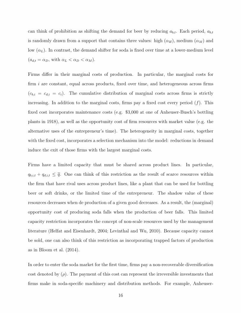
can think of prohibition as shifting the demand for beer by reducing ab,t. Each period, ab,t

is randomly drawn from a support that contains three values: high (αH), medium (αM) and

low (αL). In contrast, the demand shifter for soda is fixed over time at a lower-medium level

(ad,t = αD, with αL < αD < αM).

Firms differ in their marginal costs of production. In particular, the marginal costs for

firm i are constant, equal across products, fixed over time, and heterogeneous across firms

(cb,i = cd,i = ci). The cumulative distribution of marginal costs across firms is strictly

increasing. In addition to the marginal costs, firms pay a fixed cost every period (f). This

fixed cost incorporates maintenance costs (e.g. $3,000 at one of Anheuser-Busch’s bottling

plants in 1918), as well as the opportunity cost of firm resources with market value (e.g. the

alternative uses of the entrepreneur’s time). The heterogeneity in marginal costs, together

with the fixed cost, incorporates a selection mechanism into the model: reductions in demand

induce the exit of those firms with the largest marginal costs.

Firms have a limited capacity that must be shared across product lines. In particular,

qb,i,t + qd,i,t ≤ q. One can think of this restriction as the result of scarce resources within

the firm that have rival uses across product lines, like a plant that can be used for bottling

beer or soft drinks, or the limited time of the entrepreneur. The shadow value of these

resources decreases when de production of a given good decreases. As a result, the (marginal)

opportunity cost of producing soda falls when the production of beer falls. This limited

capacity restriction incorporates the concept of non-scale resources used by the management

literature (Helfat and Eisenhardt, 2004; Levinthal and Wu, 2010). Because capacity cannot

be sold, one can also think of this restriction as incorporating trapped factors of production

as in Bloom et al. (2014).

In order to enter the soda market for the first time, firms pay a non-recoverable diversification

cost denoted by (ρ). The payment of this cost can represent the irreversible investments that

firms make in soda-specific machinery and distribution methods. For example, Anheuser-

16

Busch used de-alcoholization machines to produce Budweiser near-beer in 1920 (Plavchan,

1969). These machines had few alternative uses other than the production of near-beer.

At the start of each period, the firm observes its survival status at the end of last period,

whether it already paid the diversification cost, and the current demand shifter for beer.

Each period, the firm makes three choices in order to maximize profits. If the firm is still

alive, the firm chooses whether to close down or survive. Exit is irreversible. If the firm has

not paid the diversification cost yet, the firm chooses whether to remain specialized on beer

or enter the soda market by paying the diversification cost. Finally, the firm chooses how

much to produce of each good.

The essence of the model comes from the interaction between two forces. On the one hand, the

fixed cost (f) generates economies of scope between the main and the alternative products.36

On the other hand, the limited plant capacity induces firms to specialize when the demand for

beer is high, because the opportunity of producing soda is too high in that case.37 Whether

the firm diversify, specialize or exit, depends on its exogenous endowment of marginal costs

(c) and the evolution of demand. Because diversification requires irreversible investments,

the history of demand reductions influences the survival of firms in the future.

Let πS(ab,t, ci) denote the static profits of a firm that has not paid the diversification cost,

and therefore can only produce beer in a given period.38 Let πD(ab,t, ci) denote the static

profits of a firm that has already paid the diversification cost, and therefore can produce

36Under regularity conditions, economies of scope are equivalent to the existence of sharable inputs betweenproducts (Panzar and Willig, 1981)

37Teece (1980) presents a more detailed discussion on how the gains from diversification are limited bycongestion and transaction costs within the firm.

38πS(ab,t, ci) is given by:

πS(ab,t, ci) = max.qb

p(qb; ab,t)qb − ciqb − f

s.t. qb ≤ q

17

both beer and sodas in a given period.39 In period 1, a firm choose to diversify, specialize or

exit depending on whether the following conditions hold:

πD(ab,1, ci) + Eab,2 [max{πD(ab,2, ci), 0}]− ρ

≥

πS(ab,1, ci) + Eab,2 [max{πS(ab,2, ci), πD(ab,2, ci)− ρ, 0}]

(1)

πD(ab,1, ci) + Eab,2 [max{πD(ab,2, ci), 0}]− ρ ≥0 (2)

πS(ab,1, ci) + Eab,2 [max{πS(ab,2, ci), πD(ab,2, ci)− ρ, 0}] ≥0 (3)

In condition 1, the profits under diversification are larger than the profits under specialization.

In condition 2, the profits under diversification are positive. In condition 3, the profits under

specialization are positive. If conditions 1 and 2 hold, the firm pays the diversification cost

and survives by producing both products in each period. If condition 1 does not hold, but

condition 3 holds, the firm survives, specializes in beer and does not pay the diversification

cost. If conditions 2 and 3 do not hold, the firm closes down.

Because profits from both soda and beer are decreasing in marginal costs, conditions 1 - 3

define thresholds of marginal costs below which firms choose to survive and diversify. These

thresholds depend on the level of demand in period 1. If beer demand is high enough, the

[marginal] opportunity cost of producing soda is too high, and most firms specialize in beer.

Decreases in beer demand liberate resources, reducing the [marginal] opportunity cost of

producing soda for diversified firms, and increasing the threshold under which condition 1

39πD(ab,t, ci) is given by:

πD(ab,t, ci) = max.qb,qd

p(qb; ab,t)qb − ciqb + p(qd; ad)qd − ciqd − f

s.t. qb + qd ≤ q

18

holds. However, reductions in demand also decrease the threshold under which the survival

condition (2) holds. For high and medium levels of demand, the first effect dominates and

there is an increase in the share of firms that diversify, unconditional on survival. For low

levels of demand, the second effect dominates and there is a decrease in the share of firms

that diversify, unconditional on survival.

In what follows, I discuss the effect of sequential reductions in beer demand on the investment

and survival decisions of firms. In particular, I compare two scenarios. In the first scenario,

firms experience an initial reduction in beer demand from αH to αM , followed by a further

reduction in beer demand from αM to αL (i.e. ab,1 = αM and ab,2 = αL). This scenario

represents the demand sequence experienced by breweries affected by local prohibition in

other counties. In the second scenario, firms do not experience an initial reduction in beer

demand, and instead experience a large reduction in beer demand from αH to αL in period

2 (i.e. ab,1 = αH and ab,2 = αL). This scenario represents the demand sequence experienced

by breweries not affected by local prohibition. In both scenarios, the demand for sodas

remain fixed at ad,t = αD. I show that the gradual reduction in beer demand (first scenario)

generates higher two-period survival rates than the sudden reduction in beer demand (second

scenario). The appendix provides restrictions in the functional form of the demand function,

as well as the parameters, for the increased survival to hold.40

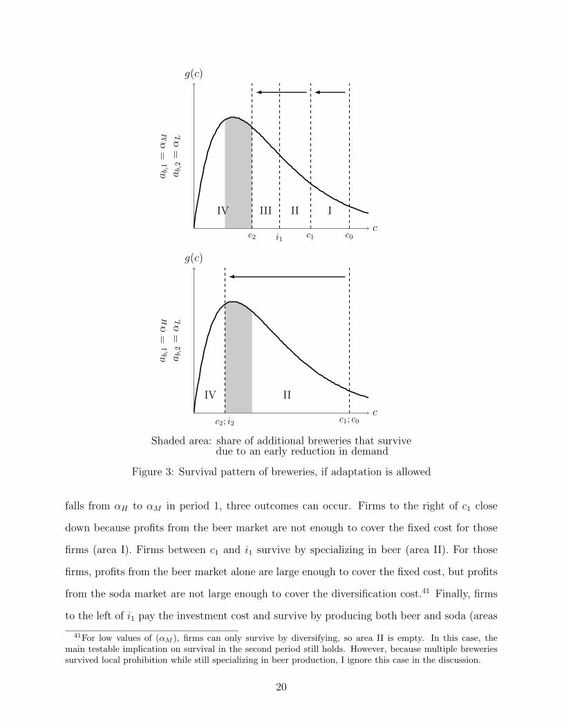
Figure 3 illustrates how survival in period 2 depends both on the level of demand experienced

by the firm in period 1 and the exogenous marginal costs of the firm. The top plot represents

the effect of a gradual reduction of demand, with ab,1 = αM and ab,2 = αL. When demand

40The main restriction on the demand function is to be additively separable on the demand shifter. Thisrestriction simplifies the expressions that result from the application of the envelope theorem on the profitfunctions when finding derivatives. Most results are based on the following (derived) properties of the staticprofit functions, which allow for single-crossing conditions throughout the proof:

∂πSab≥∂πD∂ab

≥ 0

∂πD∂ci

≤∂πS∂ci≤ 0

19

IV III II I

c2 i1 c1 c0c

g(c)

IV II

c2; i2 c1; c0c

g(c)

ab,1

=αM

ab,2

=αL

ab,1

=αH

ab,2

=αL

Shaded area: share of additional breweries that survivedue to an early reduction in demand

Figure 3: Survival pattern of breweries, if adaptation is allowed

falls from αH to αM in period 1, three outcomes can occur. Firms to the right of c1 close

down because profits from the beer market are not enough to cover the fixed cost for those

firms (area I). Firms between c1 and i1 survive by specializing in beer (area II). For those

firms, profits from the beer market alone are large enough to cover the fixed cost, but profits

from the soda market are not large enough to cover the diversification cost.41 Finally, firms

to the left of i1 pay the investment cost and survive by producing both beer and soda (areas

41For low values of (αM ), firms can only survive by diversifying, so area II is empty. In this case, themain testable implication on survival in the second period still holds. However, because multiple breweriessurvived local prohibition while still specializing in beer production, I ignore this case in the discussion.

20

III and IV). For these firms, profits in the soda market over two periods are large enough to

cover the diversification cost.

When demand falls to a low level in period 2 (ab,2 = αL), variable profits from the beer

market are too low to compensate for the fixed costs of the firms. Hence, firms can survive

only by entering the soda market. Firms with large marginal costs close down, including the

beer-specialized firms (area II) and a subset of the diversified firms (area III). Only firms

with low marginal costs remain alive. The survival rate over both periods is given by area

IV.

The bottom plot of figure 3 represents the decisions of firms that experience high demand in

the first period, followed by a sudden reduction in demand in the second period (ab,1 = αH

and and ab,2 = αL). When demand in period 1 is high, surviving firms specialize in beer

because the [marginal] opportunity cost of producing soda is too high. During period 2, the

least productive firms exit (area II), whereas the most productive firms pay the investment

cost and survive by producing both goods. The survival rate over both periods is given by

area IV.

Figure 3 also shows that there is a set of firms that survive period 2 if ab,1 = αM , but close

down if ab,1 = αH . Firms under the shaded area diversify when ab,1 = αM in period 1. When

demand is low during the second period, the diversification cost is already sunk so the firm

does not have to pay it in order to survive. In contrast, the same firms do not diversify

when ab,1 = αH in period 1, because the opportunity cost of producing soda is too high in

that period. These firms close down during period 2 because the variable profits from both

markets are not enough to cover both the fixed cost and the investment cost. Hence, under

certain values of the parameters, the share of firms that survive over both periods (area IV)

is higher when ab,1 = αM than when ab,1 = αH :

21

P (S2 = 1 | ab,1 = αM ∩ ad,2 = αL) > P (S2 = 1 | ab,1 = αH ∩ ad,2 = αL) (4)

Testable implication (4) is the result of adaptation, and does not occur when firms select

exclusively on the basis of exogenous marginal costs. To show this, I shut down the investment

channel in the model by setting ρ = 0 or ρ→∞. In the first case, diversification is costless.

In the second case, firms are unable to diversify because it is too expensive. In both cases,

the early exit of firms with large marginal costs still occurs. Yet, implication (4) does not

hold. When no adaptation is at work, the only effect of the initial demand reduction is to

induce an early exit of firms that would have exited during the second demand reduction in

any case (i.e. the firms with large marginal costs). The initial reduction in demand does not

change the behaviour of firms in the second period. Hence, when no adaptation is at work,

overall survival is not affected by the existence of an initial reduction in demand.

Figure 4 illustrates the survival decisions of firms in the absence of adaptation. In the top

plot, an initial demand reduction shifts the cost threshold to the left, inducing the exit of

firms. A subsequent demand reduction shifts the threshold further, inducing the exit of

more firms. The fraction of firms that survive both periods is given by area IV. In the

bottom plot, there is no initial reduction in demand. During period 2, a large reduction in

demand shifts the survival threshold to the left, inducing the exit of firms. Because there

are no irreversible investments, the threshold of survival at the end of period 2 does not

depend on the level of demand in period 1. Hence, the fraction of firms that survive both

periods (area IV) is the same in both plots, and implication (4) does not hold. It is still

true that, conditional on survival in period 1, the probability of survival is higher when

firms experience an initial reduction in demand (area IV divided by area II). However, the

probabilities in implication (4) are unconditional on survival in period 1 (area IV). In the

absence of adaptation, the unconditional probability of survival does not change when firms

experience an initial reduction in demand.

22

IV II I

c2 c1 c0c

g(c)

IV II

c2 c1; c0c

g(c)

ab,1

=αM

ab,2

=αL

ab,1

=αH

ab,2

=αL

Figure 4: Survival pattern of breweries, if adaptation is not allowed

The theoretical model in this section shows that firms adapt to reductions in demand by

switching to other products. When switching to other products requires irreversible invest-

ments, these investments make firms more likely to survive future reductions in demand. In

fact, overall survival can increase, as stated in implication (4). In contrast, when adaptation

through irreversible investments is not allowed, implication (4) does not hold. The remain-

ing sections of this paper show that implication (4) holds for the American brewing industry

during the Prohibition era. This result, together with additional evidence from machine ac-

quisition and product switching, confirms that adaptation was an important determinant of

brewery survival during prohibition

23

5 Empirical Strategy

In the theoretical model from last section, initial shifts in demand induce changes in the

capital structure and product scope, which can help firms survive later demand shocks.

Local prohibition induces variation in demand over time and across breweries, providing an

experimental setting to test the predictions from the theoretical model.

local prohibition shifted the demand experienced by breweries in wet counties, because they

could not ship beer to dry counties any more.42,43,44 The impact of this shift is heterogenous

across breweries, because the transportation costs to dry counties are heterogeneous as well.

A measure of the reduction in demand, therefore, has to take into account both the decisions

of the newly dry counties and the transportation costs from the breweries to those counties.

I measure the size of the demand shift at the county level by estimating the effect of local

prohibition in surrounding areas on market access. Market access is a measure of total

potential demand that is commonly used in the economic geography literature (Harris, 1954;

Head and Mayer, 2004). In trade models of differentiated products with CES preferences

across varieties and economies of scale (e.g. Redding and Venables, 2004), changes in market

access summarize the demand shifts that occur across different locations in space.45 Following

Donaldson and Hornbeck (2015), my empirical implementation of market access is a sum of

populations across counties, where each county is weighted by a function of its transportation

cost to the county where the brewery is located. However, I adapt their implementation of

42More precisely: given a price schedule across markets, breweries would sell less beer during local prohi-bition than before local prohibition. Alternatively: during local prohibition, breweries would need to reducetheir prices in wet markets in order to sell the same quantity as before local prohibition.

43Even though breweries were not able to sell beer in dry counties, they were still able to buy inputsfrom there. For example, breweries continued to buy hops from the Pacific Coast, even though most hopsproducing areas had became dry by 1916. By the time of local prohibition, the Pacific was already the leadinghops-producing area in the United States (Edwardson, 1952)

44As mentioned in the historical framework, local prohibition induces reductions in demand even if breweriessmuggle beer to dry counties, due to the costs of evading the Law and the disappearance of the maindistribution channel at destination —the saloon.

45The formula for market access can also be derived from models with homogeneous products and produc-tivity heterogeneity across firms (as in Donaldson and Hornbeck, 2015)

24

market access for the purposes of this paper. In particular, I only include wet counties as

destinations in the calculation, because beer could only be sold in wet counties.46 In addition,

I include the “home” county in the calculation, because the local market was an important

sales destination for most breweries.47 In consequence, the Wet Market Access (WMA) for

breweries located in county i in year t is defined as:

WMAi,t =∑j∈J

(Popj,tτ θh,i

)(Wetj,t) (5)

where J is the set of counties in the US, Popj,t is the population in county j in year t, and

Wetj,t is a binary variable that takes the value of one if county j was wet in year t and zero

otherwise. τi,j,t is the iceberg transportation cost between county i and county j in 1890, as

estimated by Donaldson and Hornbeck (2015) In trade models with product differentiation,

CES preferences across varieties, and economies of scale, the structural interpretation of θ is

one minus the elasticity of substitution between the different varieties of the good.48 Hence, θ

is negatively related to product differentiation in the industry of interest. With large numbers

of varieties, like in the beer industry, θ can be estimated as the elasticity of trade with respect

to trade costs. For my empirical application, I use θ = 2.55, which is the estimate of Caliendo

and Parro (2015) for the food industry. Note: For the estimations in this draft I actually

used θ = 4. I will update my estimations; I don’t think things will change, but we will see.

Wet market access can change over time for three reasons: changes in transportation costs,

changes in population, and changes in the dry status of counties. Because late local prohibi-

tion only lasted four years, I assume that transportation costs do not change. In that case,

changes in market access for breweries located in county i between year s and year t can be

46I consider the effects of beer smuggling on my estimates below47I assume that distributing beer within counties is costless, so the iceberg transportation cost from a

county to itself is one.48In models with homogeneous products and productivity heterogeneity (e.g. Eaton and Kortum, 2002;

Donaldson and Hornbeck, 2015), θ is a parameter that is inversely related to the spread of the distributionof productivities

25

decomposed as follows:

∆stWMAi = −∑j∈J

[Popj,sτ θi,j,s

]Wetj,s (1−Wetj,t)

+∑j∈J

[Popj,tτ θi,j,t

](1−Wetj,s)Wetj,t

Change due to

LocalProhibition

+∑j∈J

[(Popj,tτ θi,j,t

)−

(Popj,sτ θi,j,s

)]Wetj,sWetj,t

}Change due to

populationgrowth

(6)

The first line is the decrease in market access induced by counties that switched from wet to

dry between periods s and t. 615 counties (j) switched from wet to dry between 1914 and

1918. The second line is the increase in market access induced by counties that switched

from dry to wet between periods s and t. Only 52 counties (j) switched from dry to wet

between 1914 and 1918. The sum of the first and second line is the change in market access

induced by local prohibition, keeping population constant. The third line is the increase in

market access induced by population growth in counties (j) that remained wet throughout

the period. 489 counties remained wet throughout the period.49

local prohibition induced large reductions in market access for the counties that remained

wet between 1914 and 1918. All wet counties (489) experienced reductions in wet market

access due to local prohibition, and 408 counties experienced overall reductions in wet market

access. On average, wet counties lost 11% of their market access due to local prohibition

and experienced a 9% reduction in their overall wet market access. At the brewery level,

these average losses are 9% and 4%, respectively. Although all breweries experienced market

access losses due to local prohibition, there is large variation across space in the intensity of

the losses: 10% of breweries experienced losses in market access of 2% or less, whereas 10%

of the breweries experienced losses in market access of 19% or more.50

491570 counties, mostly rural and in the South, remained dry throughout the period50At the brewery level, the descriptive statistics of the market losses due to local prohibition are as follows.

Mean: 9%. Median: 7%. Standard deviation: 7%. Inter-quartile range: 10%. The map in Figure 5 (below)

26

My empirical strategy uses local prohibition as an instrument for decreases in market access,

allowing for the estimation of the effect of decreases in market access on changes in the capital

stock (i.e. investment), the product scope and the survival status of breweries. For each of

these outcomes (which are changes in state variables), I estimate the following system of

equations at the brewery level (Outcomeh,i denotes the outcome of brewery h in county i):

Outcomeh,i = β0 + β1 [−∆14,18ln (WMAh,i)] + uh,i (7)

[−∆14,18ln (WMAh,i)] = γ0 + γ1

[−

Change due to local prohibitionh,i,14,18WMAh,i,14

]+ vh,i (8)

where “Change due to local prohibitionh,i,14,18” is the component of the change in Wet Mar-

ket Access (WMA) that was induced by local prohibition, as defined in equation (6). From

now on, I refer to the instrument in equation (8) as “Market Access Lost to Prohibition”. The

endogenous variable [−∆14,18ln (WMAh,i)] is the log-reduction in wet market access during

the local prohibition period.

I conduct this estimation on a set of breweries that satisfies three conditions: (i) being

alive at the start of local prohibition (1914) (ii) being located in counties that remained

wet throughout local prohibition (1914-1918) and (iii) being a bottler of beer. I focus on

bottlers because the reductions in market access caused by local prohibition only had a first

order effect on breweries that shipped beer to other counties. As mentioned in the historical

overview, non-bottlers distributed their beer exclusively in kegs and were mostly focused in

local markets.51 At the start of local prohibition, 71% of the brewers were bottlers.

The main object of interest in equations (7) and (8) is β1: the effect of reductions in market

access induced by local prohibition on the outcomes of interest. I examine the following

outcomes:

shows the spatial distribution of these losses.51In the next section, I show that local prohibition had no effect within the set of non-bottlers, as expected

27

Beer-specific investment (e.g. keg washer) during local prohibition. Binary variable that takes

the value of one if the brewery acquired beer-specific machinery between 1914 and 1918, and

zero otherwise. Following the theoretical model, the predicted value of β1 is negative in

this case: reductions in market access caused by local prohibition induce reductions on the

investment in beer machinery during local prohibition.

Bottling investment during local prohibition. Binary variable that takes the value of one

if the brewery acquired bottling machinery between 1914 and 1918, and zero otherwise.

Bottling machinery can be used to produce both soda and beer. Following the theoretical

model, the predicted value of β1 is negative in this case: reductions in market access caused

by local prohibition induce reductions on the investment in bottling machinery during local

prohibition.

Soda-specific investment (e.g. carbonator) during local prohibition. Binary variable that

takes the value of one if the brewery acquired soda-specific machinery between 1914 and

1918, and zero otherwise. Following the theoretical model, the predicted value of β1 is

positive in this case: reductions in market access caused by local prohibition induce increases

on the investment in soda machinery during local prohibition.

Soda production during federal prohibition.52 Binary variable that takes the value of one if

the brewery produced sodas in 1923, and zero otherwise. Following the theoretical model,

the predicted value of β1 is negative in this case: reductions in market access caused by local

prohibition induce increases on the probability that a brewery will produce sodas during

federal prohibition.

Overall survival: Binary variable that takes the value of one if the brewery survived between

1914 and 1933, and zero otherwise. The variable is named “overall survival” because the

period 1914-1933 covers both local and federal prohibition. β1 can be positive thanks to the

52I have found no evidence that breweries were producing sodas before the start of local prohibition. Forexample, Anheuser Busch released its cereal beverage —Bevo— in 1916 (Plavchan, 1969, p. 160)

28

investments of firms during local prohibition. This is, adaptation can increase the probability

that a brewery will survive the joint period of local and federal prohibition. Very importantly,

the sample is the set of breweries alive in 1914 (at the start of local prohibition), as opposed

to the set of breweries alive in 1918 (at the start of federal prohibition).

The system of equations (7) and (8) is identified as long as the share of market access lost to

local prohibition is uncorrelated with the error term uh,i. In order to examine the plausibility

of this assumption, consider the variables included in uh,i when the outcome of interest is

overall survival.

As suggested by the theoretical model, the main component of uh,i is the exogenous com-

ponent of marginal costs/productivity of firm h at the start of local prohibition. uh,i also

contains variables that are not included in the theoretical model but that could plausibly in-

fluence survival, like the liquidity constraints that the firm faces and the prices of production

inputs. A necessary condition for identification is, therefore, that changes in local prohibition

in other counties are not correlated with these variables. In what follows, I argue that, in

my setting, the potential violations of this condition drive the estimate towards zero. Hence,

my estimates are a lower bound of the (positive) effects of local prohibition on the overall

survival of firms.

The map in Figure 5 shows, at the county level, the reduction in market access induced by

local prohibition decisions in other counties (illustrated via shading). The size of each bubble

also shows the number of breweries in each county. One possible source of concern is that local

prohibition had a smaller impact in counties with large home markets, because home markets

cushioned breweries from the local prohibition decisions of other counties. Home market size

might be positively correlated with the productivity of breweries due to the pro-competitive

effects of larger markets, lower financial constraints, or economies of agglomeration. In all

those cases, counties with large home markets will tend to have the most productive firms.

Hence, local prohibition might have had the lowest impact in those counties with the most

29

productive firms. This would generate a negative correlation between the instrument in

Equation 8 and the error term in Equation 7 This negative correlation would asymptotically

bias the estimate of β1 downwards (i.e. towards zero; given my prediction that β1 is positive).

Figure 5: Market Access Loss due to Prohibition, by county, 1914-1918

Another possibility is that the most productive breweries may have had larger resources to

make political lobby against local prohibition in nearby counties. In this case, market loss

due to local prohibition would be negatively correlated with productivity. Again, this would

bias the estimate of β1 downwards (i.e. towards zero; given my prediction that β1 is positive).

In order to check for other possible sources of endogeneity, I also run a placebo test by

estimating the model from equations (7) and (8) on the sample of non-bottlers. Supply

side factors —like within-county changes in input markets— have an effect in both bottlers

and non-bottlers. In contrast, local prohibition should not have an effect on the demand

experienced by non-bottlers, because non-bottlers did not ship beer to other counties.53 In

53Alternatively, the transportation costs for non-bottlers are too high, so my measure of market access

30

consequence, any impact on the outcomes of non-bottlers would be the result of correlations

between the instrument and the error term, or the result of second order, positive effects

through the price of factors, as in Melitz (2003)54 As it will shown below, local prohibition

does not generate variation in outcomes within the set of non-bottlers. This suggests that

the variation in outcomes within the set of bottlers is effectively generated by reductions in

demand.

6 Results

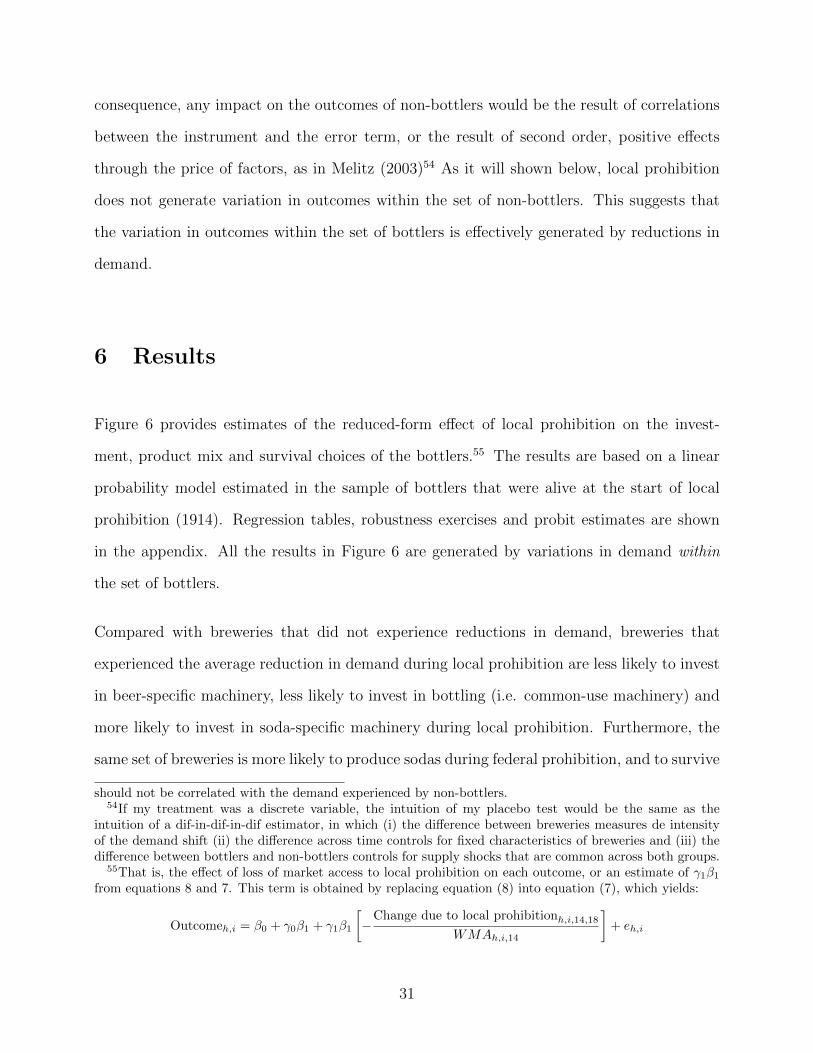
Figure 6 provides estimates of the reduced-form effect of local prohibition on the invest-

ment, product mix and survival choices of the bottlers.55 The results are based on a linear

probability model estimated in the sample of bottlers that were alive at the start of local

prohibition (1914). Regression tables, robustness exercises and probit estimates are shown

in the appendix. All the results in Figure 6 are generated by variations in demand within

the set of bottlers.

Compared with breweries that did not experience reductions in demand, breweries that

experienced the average reduction in demand during local prohibition are less likely to invest

in beer-specific machinery, less likely to invest in bottling (i.e. common-use machinery) and

more likely to invest in soda-specific machinery during local prohibition. Furthermore, the

same set of breweries is more likely to produce sodas during federal prohibition, and to survive

should not be correlated with the demand experienced by non-bottlers.54If my treatment was a discrete variable, the intuition of my placebo test would be the same as the

intuition of a dif-in-dif-in-dif estimator, in which (i) the difference between breweries measures de intensityof the demand shift (ii) the difference across time controls for fixed characteristics of breweries and (iii) thedifference between bottlers and non-bottlers controls for supply shocks that are common across both groups.

55That is, the effect of loss of market access to local prohibition on each outcome, or an estimate of γ1β1from equations 8 and 7. This term is obtained by replacing equation (8) into equation (7), which yields:

Outcomeh,i = β0 + γ0β1 + γ1β1

[−

Change due to local prohibitionh,i,14,18

WMAh,i,14

]+ eh,i

31

the overall Prohibition period, including local and federal prohibition. The latter result is

remarkable: breweries that faced five additional years of hardship were 5 percentage points

more likely to survive the entire period because they adapted earlier. This increase in survival

represents 10% of the overall survival rate of the period. All the results are consistent with

the predictions from the theoretical model.

Figure 6: Effect of local prohibition on multiple outcomes for bottlers, 1914-1933

In order to confirm that local prohibition affects outcomes through reductions in market

access, I use the share of market access lost to local prohibition as an instrument for reductions

in market access; and then estimate the effect of market access on investment, product-mix

and survival. In particular, I estimate γ1 and β1 from equations (7) and (8) using a two-

stage least-squares procedure on a linear probability model (the appendix shows robustness

exercises, including maximum likelihood estimates of β1 for a probit model).

32

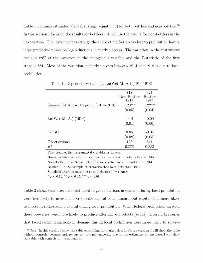
Table 1 contains estimates of the first stage (equation 8) for both bottlers and non-bottlers.56

In this section I focus on the results for bottlers —I will use the results for non-bottlers in the

next section. The instrument is strong: the share of market access lost to prohibition have a

large predictive power on log-reductions in market access. The variation in the instrument

explains 89% of the variation in the endogenous variable and the F-statistic of the first

stage is 881. Most of the variation in market access between 1914 and 1918 is due to local

prohibition.

Table 1: Dependent variable: ↓ Ln(Wet M. A.) (1914-1918)

(1) (2)Non-Bottler

1914Bottler1914

Share of M.A. lost to proh. (1914-1918) 1.20∗∗∗ 1.22∗∗∗

(0.05) (0.04)

Ln(Wet M. A.) (1914) -0.01 -0.00(0.01) (0.00)

Constant 0.05 -0.04(0.08) (0.05)

Observations 193 511R2 0.888 0.883

First stage of the instrumental variables estimates

Breweries alive in 1914, in locations that were wet in both 1914 and 1918

Non-Bottler 1914: Subsample of breweries that were no bottlers in 1914

Bottler 1914: Subsample of breweries that were bottlers in 1914

Standard errors in parentheses and clustered by county∗ p < 0.10, ∗∗ p < 0.05, ∗∗∗ p < 0.01

Table 2 shows that breweries that faced larger reductions in demand during local prohibition

were less likely to invest in beer-specific capital or common-input capital, but more likely

to invest in soda-specific capital during local prohibition. When federal prohibition arrived,

these breweries were more likely to produce alternative products (sodas). Overall, breweries

that faced larger reductions in demand during local prohibition were more likely to survive

56Note: In this version I show the table controlling for market size. In future versions I will show the tablewithout controls, because endogenous controls may generate bias in the estimates. In any case, I will showthe table with controls in the appendix.

33

the whole period, including local and federal prohibition.57

The results in this section all point in the same direction: bottlers adapted to local prohibition

by investing in capital that provided flexibility later, when federal prohibition arrived. As

a result, bottlers that faced reductions in demand during the local prohibition period were

more likely to survive the whole period, including local and federal prohibitions.

57All dependent variables in table 2 only take the values of 0 or 1.

34

Table 2: Bottlers: Effect of reductions in market access

Beer-SpecificInvestment(Local P.)

Common InputInvestment(Local P.)

Soda-SpecificInvestment(Local P.)

Soda production(Federal P.)

SurvivalFrom: Start of Local P.To: End of Federal P.

↓ Ln(Wet M. A.) (1914-1918) -0.27∗ -0.42∗ 0.25∗ 0.69∗∗∗ 0.49∗

(0.15) (0.22) (0.14) (0.24) (0.26)

Ln(Wet M. A.) (1914) 0.04∗∗∗ 0.06∗∗∗ -0.01 -0.03∗ 0.04∗∗

(0.01) (0.01) (0.01) (0.02) (0.02)

Constant -0.35∗∗∗ -0.48∗∗∗ 0.24∗ 0.63∗∗∗ 0.01(0.10) (0.17) (0.13) (0.21) (0.23)

Observations 511 511 511 511 511

Instrumental variables estimates. Instrument: Share of M.A. lost to proh. (1914-1918)

Breweries alive in 1914, in locations that were wet in both 1914 and 1918

Standard errors in parentheses and clustered by county∗ p < 0.10, ∗∗ p < 0.05, ∗∗∗ p < 0.01

35

7 Placebo Test

My results from last section rely on the interpretation of local prohibition as a demand

reduction for the bottlers. In turn, this interpretation relies on an identification assumption:

prohibition decisions in nearby counties are uncorrelated with the productive amenities where

the breweries are located. I provide empirical support for that assumption by running the

same regressions on the set of non-bottlers.

Most non-bottlers did not ship beer to other counties. In consequence, exposure to local

prohibition should not induce (first-order) variation in demand within the set of non-bottlers.

However, if exposure to local prohibition were correlated with productive amenities, changes

in wet market access would capture the effect of productive amenities on non-bottlers.

Figure 7 shows that exposure to local prohibition had no effect on investment, product-

mix or survival among non-bottlers. This result sugggests that the changes in investment,

product-mix and survival among bottlers were induced by a shift in demand, as opposed to

differences in productive amenities among the bottlers.

Figure 7: Effect of local prohibition on multiple outcomes for Non-bottlers, 1914-1933

36

8 Conclusions

This paper shows that demand reductions in the early history of a firm can affect its tra-

jectory and response to future demand reductions. In particular, exposure to small demand

reductions can make firms more resilient to future, potentially larger demand reductions

by encouraging firms to make investments that facilitate product switching. I reach this

conclusion by studying the American brewing industry during prohibition.

This historical context allows me to follow breweries throughout an initial shock of heteroge-

neous intensity (local prohibition), followed by a common, larger, shock (federal prohibition).

By studying survival throughout both shocks, I show that adaptation –the making of irre-

versible investments in response to the first shock– increases the ability of firms to survive the

second shock, even if selection –the exit of the least productive firms– also occurs in response

to the first shock. My novel dataset on machinery acquisition and product diversification

corroborates the testable implications of the adaptation mechanism.

The key components of my mechanism –irreversible investments and multi-product firms–

are present in many industries of today. For example, firms that span multiple industries

account for 81 percent of the manufacturing output and 28 percent of the number firms in

the US (Bernard et al., 2010).58

Firms in these industries can experience reductions in demand due to regulation, trade re-

forms, and sectoral changes in government spending. Policy makers often care about the sur-

vival of firms for its own sake, due to political economy considerations or possible externalities

induced by firm exit. My results suggest that increased gradualism in the implementation of

these policies can facilitate the adaptation and survival of firms to the policy at hand.

58Industries are defined as four-digit SIC categories in the US manufacturing census (ibid).

37

References

Agarwal, R. and Helfat, C. E. (2009). Strategic renewal of organizations. Organization

Science, 20(2):281–293.

Aggarwal, V. A. and Wu, B. (2015). Organizational constraints to adaptation: Intrafirm

asymmetry in the locus of coordination. Organization Science, 26(1):218–238.

Aghion, P., Bloom, N., Lucking, B., Sadun, R., and van Reenen, J. (2015). Growth and

decentralization in bad times. Working paper.

Arnold, J. and Penman, F. (1933). History of the Brewing Industry and Brewing Science in

America. BeerBooks.com. Reprinted in 2006.

Atack, J. (2013). On the use of geographic information systems in economic history:

The american transportation revolution revisited. The Journal of Economic History,

73(02):313–338.

Baron, S. (1962). Brewed in America: a history of beer and ale in the United States. Little,

Brown.

Beman, L. (1927). Selected Articles on Prohibition: Modification of the Volstead Law. Sup-

plement. Number v. 2 in Reference shelf. Wilson.

Bernard, A. B., Redding, S. J., and Schott, P. K. (2010). Multiple-product firms and product

switching. American Economic Review, 100(1):70–97.

Bernard, A. B., Redding, S. J., and Schott, P. K. (2011). Multiproduct firms and trade

liberalization. The Quarterly Journal of Economics, 126(3):1271–1318.

Bloom, N., Draka, M., and van Reenen, J. (2015). Trade induced technical change: The

impact of chinese imports on innovation, diffusion and productivity. Review of Economic

Studies.

Bloom, N., Romer, P. M., Terry, S. J., and Reenen, J. V. (2014). Trapped factors and china’s

impact on global growth. Working paper.

Bresnahan, T. F. and Raff, D. M. G. (1991). Intra-Industry Heterogeneity and the Great

Depression: The American Motor Vehicles Industry, 1929-1935. The Journal of Economic

History, 51(2):pp. 317–331.

Bureau of Internal Revenue (1905). Annual Report for the Commissioner of Internal Revenue.

Number 2424 in Document. Government Printing Office. Fiscal Year Ended June 30, 1905.

38

Bureau of Internal Revenue (1922). Annual Report for the Commissioner of Internal Revenue.

Government Printing Office. Fiscal Year Ended June 30, 1922.

Bureau of Internal Revenue (1923). Annual Report for the Commissioner of Internal Revenue.

Number 2929 in Document. Government Printing Office. Fiscal Year Ended June 30, 1923.

Caballero, R. J. and Hammour, M. L. (1994). The Cleansing Effect of Recessions. The

American Economic Review, 84(5):pp. 1350–1368.

Caliendo, L. and Parro, F. (2015). Estimates of the trade and welfare effects of nafta. The

Review of Economic Studies, 82(1):1–44.

Chandler, A. (1990). Scale and Scope: The Dynamics of Industrial Capitalism. Belknap

Press.

Cochran, T. C. (1948). The Pabst Brewing Company: the History of an American Business.

New York University Press.

Dewatripont, M. and Roland, G. (1992). Economic reform and dynamic political constraints.

The Review of Economic Studies, 59(4):703–730.

Dewatripont, M. and Roland, G. (1995). The design of reform packages under uncertainty.

The American Economic Review, 85(5):pp. 1207–1223.

Donaldson, D. and Hornbeck, R. (2015). Railroads and american economic growth: A ”mar-

ket access” approach. Working paper.

Eaton, J. and Kortum, S. (2002). Technology, Geography, and Trade. Econometrica,

70(5):1741–1779.

Edwardson, J. (1952). Hopstheir botany, history, production and utilization. Economic

Botany, 6(2):160–175.

Feldman, H. (1927). Prohibition, its economic and industrial aspects. D. Appleton and

company, New York, London.

Fogel, R. W. (1964). Railroads and American economic growth: essays in econometric history,

volume 296. Johns Hopkins Press Baltimore.

Foster, L., Grim, C., and Haltiwanger, J. (2014). Reallocation in the great recession: Cleans-

ing or not? Working Paper.

39

Fox, H. and Hoyt, W. (1852). Fox and Hoyt’s Quadrennial Register of the Methodist Episcopal

Church: And Universal Church Gazetteer, 1852-6. Case, Tiffany & Company.

Freiman, R. B. and Kleiner, M. M. (2005). The last american shoe manufacturers: Decreas-

ing productivity and increasing profits in the shift from piece rates to continuous flow

production*. Industrial Relations: A Journal of Economy and Society, 44(2):307–330.

Fujita, M., Krugman, P. R., and Venables, A. (2001). The Spatial economy: Cities, regions,

and international trade. MIT press.

Garcıa-Jimeno, C. (2015). The political economy of moral conflict: An empirical study of

learning and law enforcement under prohibition. Working paper.

Gohmann, S. F. (2015). Why are there so few breweries in the south? Entrepreneurship

Theory and Practice, pages n/a–n/a.

Harris, C. D. (1954). The market as a factor in the localization of industry in the united

states. Annals of the Association of American Geographers, 44(4):pp. 315–348.

Head, K. and Mayer, T. (2004). Chapter 59 the empirics of agglomeration and trade. In

Henderson, J. V. and Thisse, J.-F., editors, Cities and Geography, volume 4 of Handbook

of Regional and Urban Economics, pages 2609 – 2669. Elsevier.

Helfat, C. E. and Eisenhardt, K. M. (2004). Inter-temporal economies of scope, organizational

modularity, and the dynamics of diversification. Strategic Management Journal, 25(13):pp.

1217–1232.

Hiatt, S. R., Sine, W. D., and Tolbert, P. S. (2009). From pabst to pepsi: The deinstitutional-

ization of social practices and the creation of entrepreneurial opportunities. Administrative

Science Quarterly, 54(4):635–667.

Holmes, T. J., Levine, D. K., and Schmitz, J. A. (2012). Monopoly and the incentive to

innovate when adoption involves switchover disruptions. American Economic Journal:

Microeconomics, 4(3):1–33.

Hopenhayn, H. A. (1992). Entry, exit, and firm dynamics in long run equilibrium. Econo-

metrica, pages 1127–1150.

H.S. Rich & Co. (1923). The Beverage Blue Book 1923. H.S. Rich & Co.

Kerr, K. (1985). Organized for Prohibition: A New History of the Anti-Saloon League. Yale

University Press.

40

Kerr, K. A. (1998). The american brewing industry, 1865-1920. In Wilson, R. and Gourvish,

T., editors, The Dynamics of the International Brewing Industry Since 1800, chapter 11,

pages 176 – 192. Routledge.

Leamer, E. E. (1980). The leontief paradox, reconsidered. Journal of Political Economy,

88(3):pp. 495–503.

Legislative Research Commission of Kentucky (2015). The constitution of the commonwealth

of kentucky. Frankfort, Kentucky.

Levinthal, D. A. and Wu, B. (2010). Opportunity costs and non-scale free capabilities:

profit maximization, corporate scope, and profit margins. Strategic Management Journal,

31(7):780–801.

Maxwell, D. B. S. (1993). Beer cans: A guide for the archaeologist. Historical Archaeology,

27(1):pp. 95–113.

Maxwell, H. and Sullivan, B. (1999). Hometown Beer: A History of Kansas City’s Breweries.

Omega Innovative Marketing.

McGahan, A. M. (1991). The emergence of the national brewing oligopoly: Competition in

the American market, 1933-1958. The Business History Review, 65(2):pp. 229–284.

Medina, P. (2015). Within-firm responses to import competition: Quality upgrading and

exporting in the peruvian apparel industry. Working paper.

Melitz, M. J. (2003). The Impact of Trade on Intra-Industry Reallocations and Aggregate

Industry Productivity. Econometrica, 71(6):pp. 1695–1725.

Minnesota Population Center (2011). National historical geographic information system:

Version 2.0. Url: https://www.nhgis.org/. Accessed: 2015-06-29.

Panzar, J. C. and Willig, R. D. (1981). Economies of scope. The American Economic Review,

71(2):pp. 268–272.

Penrose, E. (1959). The Theory of the Growth of the Firm. Oxford: Oxford University Press,

4th ed (2009) edition. Retrieved 28 Aug. 2015, from http://www.oxfordscholarship.

com/view/10.1093/0198289774.001.0001/acprof-9780198289777.

Plavchan, R. J. (1969). A history of Anheuser-Busch, 1852-1933. PhD thesis, St. Louis

University.

41

Porter, M. (1990). The Competitive Advantage of Nations. Free Press.

Porter, M. (1996). America’s green strategy. In Welford, R. and Starkey, R., editors, Business

and the Environment: A Reader, pages 33–35. Taylor & Francis Washington, DC.

Redding, S. and Venables, A. J. (2004). Economic geography and international inequality.

Journal of International Economics, 62(1):53 – 82.

Ronnenberg, H. W. (1998). The american brewing industry since 1920. In Wilson, R. and

Gourvish, T., editors, The Dynamics of the International Brewing Industry Since 1800,

chapter 11, pages 176 – 192. Routledge.

Rowntree, J. and Sherwell, A. (1900). The Temperance Problem and Social Reform. Hodder

and Stoughton.

Sechrist, R. P. (1986). A Comparative Analysis of Multidimensional Diffusion Models: The

Diffusion of the Prohibition Movement in the United States of America, 1876-1919. PhD

thesis, Louisiana State University.

Sechrist, R. P. (2012). Prohibition movement in the United States, 1801-1920. Url: http:

//www.icpsr.umich.edu/icpsrweb/ICPSR/studies/08343/version/2. Accessed: 2013-

06-29.

Southern Baptist Convention (1896). Resolution. http://www.sbc.net/resolutions/46/

untitled. Online; accessed 2015/07/17.

Stack, M. (2000). Local and regional breweries in America’s brewing industry, 1865 to 1920.

The Business History Review, 74(3):pp. 435–463.

Stack, M. (2010). Was big beautiful? the rise of national breweries in America’s pre-

prohibition brewing industry. Journal of Macromarketing, 30(1):50–60.

Steinwender, C. (2015). The roles of import competition and export opportunities for tech-

nical change. Working paper.

Teece, D. J. (1980). Economies of scope and the scope of the enterprise. Journal of Economic

Behavior & Organization, 1(3):223 – 247.

Teece, D. J., Pisano, G., and Shuen, A. (1997). Dynamic capabilities and strategic manage-

ment. Strategic Management Journal, 18(7):pp. 509–533.

Tremblay, V. and Tremblay, C. (2005). The U.S. Brewing Industry: Data and Economic

Analysis. MIT Press.

42

United States Brewers’ Association (1907). Proceedings of the Annual Convention. United

States Brewers’ Association.

United States Bureau of the Census (1907). Manufactures 1905. United States by Industries,

volume 1 of Manufactures, 1905. U.S. Government Printing Office.

United States Bureau of the Census (1908). Manufactures 1905. Special Reports on Selected

Industries, volume 3 of Manufactures, 1905. U.S. Government Printing Office.

United States Bureau of the Census (2000). Historical national population es-

timates. Url: http://www.census.gov/popest/data/national/totals/pre-1980/

tables/popclockest.txt. Accessed: 2015-06-29.

Wade, J. B., Swaminathan, A., and Saxon, M. (1998). Normative and Resource Flow Conse-

quences of Local Regulations in the American Brewing Industry, 1845-1918. Administrative

Science Quarterly, 43(4):pp. 905–935.

Wahl, R. and Henius, M., editors (1898). Brewers’ Guide. American Brewers’ Review.

43