Abstract

Adaptation in Estimation and Annealing

Sabyasachi Chatterjee

2014

We study general penalized log likelihood procedures and propose Information

Theoretic conditions required of the penalty to obtain adaptive risk bounds.

We demonstrate our conditions are natural and are satisfied in some canoni-

cal problems in statistics. We then investigate whether penalties are always

required to obtain adaptation in the rates of estimation for M estimators.

We show that the plain least squares estimators, without any penalization,

in certain canonical shape-constrained regression problems indeed adapt to

certain parametric complexities in the parameter space. We attempt to give

a geometric characterization of this adaptation behaviour. We then move on

to the important issue of computation. Motivated by a classical function es-

timation problem in non-parametric statistics, we study the possibility of a

randomized algorithm, inspired by Simulated Annealing, being able to opti-

mize multimodal functions in high dimensions. We explore the performance

of this algorithm in low dimensions and explain the challenges faced in high

dimensions. We provide myriads of possible routes for solving the statistically

relevant optimization problem with the hope of encouraging further research

in this direction.

Adaptation in Estimation and

Annealing

A DissertationPresented to the Faculty of the Graduate School

ofYale University

in Candidacy for the Degree ofDoctor of Philosophy

bySabyasachi Chatterjee

Dissertation Director: Andrew Barron

December 2014

Copyright c© 2014 by Sabyasachi Chatterjee

All rights reserved.

ii

Acknowledgements

I am deeply indebted to my advisor Professor Andrew Barron for my intellec-

tual and professional growth in the field of Statistics and other related fields.

I have benefited greatly from having spent numerous discussion sessions with

him. He has been kind enough to share his vast knowledge of the fields of

Statistics and Information Theory and I would like to think I have inculcated

in myself some of his philosophies and style of advancing research in our field.

I have also been influenced greatly by Professor David Pollard. He, again,

has been kind enough to listen to some of my research efforts and have given

me very valuable inputs and suggestions. I have also learnt a lot from the

courses he has taught me in Probability and Statistics and his constant efforts

to simplify exposition of complicated mathematical arguments is something I

will attempt to practice in the future. I also want to thank Prof. Harrison

Zhou, Prof. Joseph Chang, Prof. Sekhar Tatikonda, Prof. Sahand Negahban

and Prof. Mokshay Madiman for encouraging me and lending a helpful ear to

me whenever I wanted to talk to them.

I have had some very good friends here at Yale without whom life would not

have been the same here. I would not be able to mention all of them here.

However, I would like to mention some of the people with whom I have perhaps

spent most of my time. I would like to thank Adityanand Guntuboyina for

iii

being an exemplary role model and not the least, for introducing the problem

of adaptation in monotone regression to me. I also thank Antony Joseph and

Anup Rao for being great friends and tolerating me throughout my endless

rants and complaints. I also thank all these three people for spending numerous

hours with me on the squash and tennis courts and the various restaurants

around the great town of New Haven. I thank Rajarshi Mukherjee and Wan

Chen Lee for always being ready to give me company whenever I travelled

to Boston and for all the wonderful game nights and the travels we have had

together. Finally, I thank Dolon Bhattacharyya for being with me throughout

and travelling this journey together.

iv

Dedicated to my parents

v

Preface

Statistical methodologies have to be judged on two parameters. Firstly, their

risk and predictive properties and secondly the potential to actually implement

these methodologies using reasonable computational resources and time. In

my dissertation I have focussed on both these issues, with more emphasis

on the risk properties of estimators achieved by minimizing certain objective

functions arising from data. I have worked on three topics and I have included

them as the next three chapters in this dissertation.

Chapter 1 is on the Information Theoretic treatment of Penalized Likelihoods

and derivation of general adaptive risk bounds for the penalized likelihood

procedure. This is joint work with my advisor Andrew Barron. We develop

a general framework for studying the penalized likelihood estimator and show

that traditional penalties such as the `0 and `1 penalties in canonical statistical

problems fit our framework.

Chapter 2 is on the study of the least squares estimator in certain shape-

constrained regression problems. This work is done jointly with Adityanand

Guntuboyina and Bodhisattva Sen. We develop improved risk bounds in these

shape constrained problems and show adaptivity of the least squares estimator

for certain parametric simplicities in the parameter space.

Chapter 3 deals with computational issues and considers a multimodal op-

vi

timization problem in moderate to high dimensions motivated by a classical

function estimation problem. This is again, jointly done with my advisor

Andrew Barron. The optimization problem considered is very hard to solve

because of multimodality in high dimensions. We explore an algorithm here

which tries to improve the traditional Simulated Annealing idea. The main

difference with Simulated Annealing and our algorithm is that while the Sim-

ulated Annealing algorithm makes transition steps based on the idea of an

invariant or stationary distribution, we are inspired from the theory of Diffu-

sion processes and attempt to solve a partial differential equation known as

the Fokker Plank equation for our transition moves. While we do not claim

we have been successful completely in our efforts in this direction, nevertheless

it is an interesting idea and deserved to be pursued. It may look like these

three topics are distinct entities but as I reveal now, there have been two main

themes or threads which has driven the research in these three topics.

The first connecting thread concerns problems where we have a dictionary

of functions or candidates to linearly combine and form estimates in a den-

sity estimation or regression setting. The work in Chapter 1 reveals the risk

properties of choosing such estimators by penalizing for the complexity of the

linear combination, which could be the number of non-zero coefficients needed

to describe the parameter or the sum of absolute values of all the coefficients

of the dictionary functions. It is nice to know the good risk properties of such

estimators but we also need to compute them. If the number of dictionary ele-

ments is large but manageable such as a couple of million or so, as can happen

in high-dimensional linear regression for example, then these estimators can

be computed by looping over all elements of the dictionary by certain greedy

algorithms. In the case when the dictionary elements are indeed too large to

be looped over, as it happens in genuine non-parametric function estimation

vii

problems in high dimensions, one needs flexible algorithms with some theoret-

ical guarantees. The greedy algorithm that can be used in this case requires

us to solve a non-convex multimodal optimization problem in each step which

is precisely the motivation for our work described in Chapter 3. In this way

we see that Chapter 1 and 3 are indeed two parts of one single puzzle.

The second theme which runs through my dissertation is the notion of con-

structing adaptive risk bounds. Chapter 1 reveals what are the conditions

needed for a penalty function so that the resulting penalized likelihood esti-

mator has risk upper bounded by a Information Theoretic quantity which is

the minimum expected coding redundancy per symbol. This also permits us

to prove that the risk bounds are adaptive, that is, the estimator adapts to the

complexity of the parameter. The risk will be better for simpler elements of the

parameter space. In Chapter 2 we show a very interesting fact. For parameter

spaces which are polyhedral cones in euclidean space, the least squares esti-

mator, without any need for penalization, adapts to certain parametric com-

plexities of the parameter space. This applies to problems such as Monotone

and Convex regression. This fact seems unique to shape-constrained problems

and according to my opinion, is not very well understood yet. It seems the

geometry of these particular cones plays a role and the truth being in a low

dimensional face of these cones is advantageous as far as risk bounds for the

least squares estimator is concerned. The fundamental question of what type

of penalties are needed for adaptive estimation and when they may not be

needed, drives the research that I describe in Chapters 1 and 2.

viii

Contents

List of Figures xi

1 Information Theory of Penalized Likelihoods 1

1.1 Introduction . . . . . . . . . . . . . . . . . . . . . . . . . . . . 2

1.1.1 Notational Conventions . . . . . . . . . . . . . . . . . . 6

1.2 General Technique . . . . . . . . . . . . . . . . . . . . . . . . 7

1.2.1 Codelength validity . . . . . . . . . . . . . . . . . . . . 7

1.2.2 Risk Validity . . . . . . . . . . . . . . . . . . . . . . . 10

1.3 Validity of the l1 penalty . . . . . . . . . . . . . . . . . . . . . 21

1.3.1 Linear Regression . . . . . . . . . . . . . . . . . . . . . 22

1.3.2 Gaussian Graphical Models . . . . . . . . . . . . . . . 30

1.4 Validity of l0 penalty in Linear Regression . . . . . . . . . . . 36

1.4.1 Codelength Validity . . . . . . . . . . . . . . . . . . . . 37

1.4.2 Risk validity . . . . . . . . . . . . . . . . . . . . . . . . 44

1.5 Conclusion . . . . . . . . . . . . . . . . . . . . . . . . . . . . . 48

ix

1.6 Appendix . . . . . . . . . . . . . . . . . . . . . . . . . . . . . 48

1.6.1 Proof of Lemma (1.3.1) . . . . . . . . . . . . . . . . . . 48

1.6.2 Proof of Lemma (1.4.1) . . . . . . . . . . . . . . . . . 52

1.6.3 Proof of Lemma (1.4.3) . . . . . . . . . . . . . . . . . . 54

1.6.4 Proof of Lemma (1.4.4) . . . . . . . . . . . . . . . . . . 57

2 Improved Risk Bounds in Monotone Regression and other

Shape Constraints 63

2.1 Introduction . . . . . . . . . . . . . . . . . . . . . . . . . . . . 64

2.2 Our risk bound . . . . . . . . . . . . . . . . . . . . . . . . . . 73

2.3 The quantity R(n; θ) . . . . . . . . . . . . . . . . . . . . . . . 79

2.4 Local minimax optimality of the LSE . . . . . . . . . . . . . . 84

2.4.1 Uniform increments . . . . . . . . . . . . . . . . . . . . 86

2.4.2 Piecewise constant . . . . . . . . . . . . . . . . . . . . 90

2.5 Risk bound under model misspecification . . . . . . . . . . . . 94

2.6 A general result . . . . . . . . . . . . . . . . . . . . . . . . . . 98

2.6.1 Proof of Theorem 2.6.1 . . . . . . . . . . . . . . . . . . 104

2.7 Some auxiliary results . . . . . . . . . . . . . . . . . . . . . . 109

3 Advances in Adaptive Annealing 116

3.1 Introduction and Motivation . . . . . . . . . . . . . . . . . . . 117

x

3.1.1 Statistical Motivation . . . . . . . . . . . . . . . . . . . 117

3.1.2 Approximate Diffusion for Optimization . . . . . . . . 118

3.2 Error from Discretization . . . . . . . . . . . . . . . . . . . . . 123

3.3 Variable Augmentation Formulation . . . . . . . . . . . . . . . 125

3.4 Some Solutions of Fokker Plank and Simulations . . . . . . . . 130

3.4.1 Solution in 1 Dimension . . . . . . . . . . . . . . . . . 130

3.4.2 Extension to higher dimensions? . . . . . . . . . . . . . 132

3.4.3 Simulations in 1 dimension . . . . . . . . . . . . . . . . 135

3.4.4 Sampling in 2 dimensions . . . . . . . . . . . . . . . . 141

3.4.5 Simulations in 2 dimensions . . . . . . . . . . . . . . . 142

3.5 Sampling Multivariate Gaussians and extensions . . . . . . . . 145

3.6 Conclusion . . . . . . . . . . . . . . . . . . . . . . . . . . . . . 150

3.7 Appendix . . . . . . . . . . . . . . . . . . . . . . . . . . . . . 150

3.7.1 Proof of Lemma (3.3.1) . . . . . . . . . . . . . . . . . . 150

xi

List of Figures

3.1 Objective Function . . . . . . . . . . . . . . . . . . . . . . . . 136

3.2 Histograms . . . . . . . . . . . . . . . . . . . . . . . . . . . . 138

3.3 Trajectories with various starting points . . . . . . . . . . . . 139

3.4 Sampling from a mixture of Gaussians . . . . . . . . . . . . . 144

xii

Chapter 1

Information Theory of

Penalized Likelihoods

We extend the correspondence between two-stage coding procedures in data

compression and penalized likelihood procedures in statistical estimation. Tra-

ditionally, this had required restriction to countable parameter spaces. We

show how to extend this correspondence in the uncountable parameter case.

Leveraging the description length interpretations of penalized likelihood pro-

cedures we devise new techniques to derive adaptive risk bounds of such proce-

dures. We show that the existence of certain countable subsets of the parame-

ter space implies adaptive risk bounds and thus our theory is quite general. We

apply our techniques to illustrate risk bounds for `1 type penalized procedures

in canonical high dimensional statistical problems such as linear regression and

Gaussian graphical Models. In the linear regression problem, we also demon-

strate how the traditional l0 penalty plus lower order terms has a two stage

description length interpretation and present risk bounds for this penalized

likelihood procedure.

1

1.1 Introduction

There are close connections between good data compression and good estima-

tion in statistical settings. Shannon’s recipe for finding the minimum expected

codelength when we know the data generating distribution shows the corre-

spondence between probability distributions on data and optimal codelengths

on the sample space. Also, Kraft’s inequality stating that for every proba-

bility mass function there exists a prefix free code with lengths expressible

as minus log probability gives an operational meaning to probability. The

Kraft inequality allows one to think of prefix free codes and probabilities in-

terchangeably. The MDL principle has further developed this connection by

considering the case where we do not necessarily know the data generating

distribution. In the MDL framework codes are always meant to be prefix free.

In this framework one considers a family of codes or equivalently a set of prob-

ability distributions, possibly indexed by a parameter space Θ. The idea in one

shot data compression is to compress the observed data sequence well. But

for statistical purposes, we also want to devise a coding or estimation strategy

based on the observed data that should compress or predict well for future

data assumed to be arising from the same generating distribution.

A fundamental concept in the MDL philosophy is that of universal coding or

modelling. The aim of universal coding or modelling is to find a single code

that allows us to compress data almost as well as the best code in our class of

codes Θ either in expectation or high probability with respect to the generation

of the data X. This universal distribution can be constructed mainly in four

different ways as described in [4]. These four ways can be categorized as Two-

stage codes, Bayes mixture codes, Predictive codes and Normalized Maximum

Likelihood codes. Penalized minus log likelihood on uncountable spaces Θ

2

provides another category of universal codes as we develop here, by relating it

to Two-stage codes on appropriately defined countable subsets of Θ.

One of the earliest ways to build a universal code is to build what is called a

two stage code [1]. The basic idea is to first devise a code or description of all

the possible codes in Θ. Also for each possible code one encodes or describes

the data using that code. Then one chooses the code which minimizes the sum

of the two descriptions, one describing the code and the other describing data

given the code. Now one can play the same game in the learning setup where

now the codes are replaced by a family of probability distributions and the

estimated probability distribution is the one which minimizes the sum of the

two descriptions. This is indeed the penalized likelihood estimator where the

penalty corresponds to the description lengths of probability distributions in

our model. Traditionally, there have been various kinds of penalties that have

been proposed. Firstly, penalties which penalize roughness or irregularity of

the density as in [15],[22] and [21] have been considered. Secondly, penalties

could be generally of the `2 type. Reproducing kernel Hilbert space penal-

ties are championed in [23]. Statistical risk rate results for general quadratic

penalties in Hilbert space settings which correspond to weighted `2 norms

on coefficients in function expansions, including, in particular, Sobolev-type

penalties (squared L2 norms of derivatives) are developed in [14] and [13] based

on functional analysis tools. Empirical process techniques for penalized likeli-

hood built around metric entropy calculations are used to yield rate results for

penalties designed for a wide variety of function classes in [20]. Theory related

to penalized likelihood is developed for constrained maximum likelihood in

nonparametric settings [19] and for minimum contrast estimators and sieves

as in [11] and [12]. A general treatment of penalized likelihoods has been given

in [26]. The authors there too give sufficient conditions, namely the decom-

3

posabiltiy and the restricted strong convexity condition on the penalty and

the term corresponding to the log likelihood respectively, to obtain sharp risk

bounds. For log likelihood penalization, it would be interesting to examine if

there are connections between their conditions and the conditions proposed in

this manuscript. General oracle type bounds in problems like high dimensional

linear regression for the `1 penalty can be obtained by the method of aggrega-

tion as developed by Tsybakov and others [27]. These results have the leading

constant 1 in the oracle inequalities. Our risk bounds do not achieve the lead-

ing constant 1 but can achieve a constant arbitrarily close to 1. Nevertheless,

our work demonstrates the information theoretic side of penalized likelihood

estimators and provides another framework to study penalized likelihood pro-

cedures. There has also been a lot of activity recently on investigating the risk

rate results for `1 type penalties, including the Lasso estimator and it is indeed

a daunting task to write down all the required references. A nice survey article

in this topic where the major advancements and references can be found is [7].

Our treatment of penalized likelihoods extend the pattern of past MDL work.

Traditionally, the statistical properties of this penalized likelihood procedure

has been studied in the countable parameter space setting. Past work as in [2]

and [3] shows how the expected pointwise redundancy controls the statistical

risk in countable parameter spaces. For suitable penalties the performance is

captured by an index of resolvability which is the minimum sum of relative

entropy approximation error and the penalty relative to the sample size. Such

results have been developed previously for the case that the function fits are

restricted to a countable set which discretizes the parameter space, with a

complexity penalty equal to an information-theoretic codelength for the dis-

cretized set as in [1], [9], [18], [16] and [17]. These estimators can also be

interpreted as a maximum posterior probability estimator with the penalty

4

equal to a log reciprocal prior probability for the countable set. Resolvability

bounds on risk have also been developed for the case that the function fits

are optimized over a list of finite-dimensional families with penalty typically

proportional to the dimension as in [25] and [10].

One of the main contributions of this present manuscript is to extend such risk

bounds when the parameter space is uncountable maintaining the description

length interpretation. The main idea here is to construct countable subsets

of the parameter space Θ and leverage the results from the countable case.

These subsets are constructed according to the interaction of the minus log

likelihood and the penalty as is made clear in section (1.2.2). We show that the

loss function we consider, is not much more than the pointwise redundancy,

both in expectation and with high probability. As we would see, these risk

bounds that we get also reveal the adaptation properties of these penalized

likelihood procedures.

The main idea is to propose conditions on the penalty and the negative log

likelihood in a general setting to derive adaptive risk bounds as long as the

penalized likelihood estimator mirrors the construction of a two stage code.

In a preliminary form, this idea has appeared in [2] and [3]. This manuscript

lays out this general theory in more detail and then shows that our conditions

are satisfied and our risk bounds are valid in canonical high-dimensional sta-

tistical problems such as linear regression and inverse covariance estimation in

Gaussian models.

In section (1.2) we describe the general technique of how to relate penalized

negative log likelihoods in the uncountable parameter space case to two stage

description lengths on a appropriate countable subset. We also lay out the

general strategy for deriving adaptive risk bounds whenever the codelength re-

5

lation holds. In this section, we describe the conditions needed on the penalty

and the negative log likelihood which allows us to prove risk bounds. In Sec-

tion (1.3) we apply our theory to the `1 penalty in linear regression case and

fully illustrate different ways of verifying the conditions we need. We then

present a new result on inverse covariance matrix estimation in a multivariate

Normal setting which shows that our theory can handle not just location type

problems but scale problems as well. In Section (1.4) we then turn our atten-

tion to the `0 penalty in the linear regression case. We devise a new way to

interpret the `0 penalty times a log(n)/2 factor as Kraft satisfying codelengths

and leverage this interpretation to recover adaptive risk bounds. The penal-

ties we consider in this manuscript are traditionally two of the most commonly

used in statistics, namely the `0 penalty or the number of parameters times a

suitable multiplier and `1 type penalties with suitable multipliers.

1.1.1 Notational Conventions

We denote a general sample space by U and its elements by u. In cases when

the data is generated in an i.i.d fashion we set U = X n for some positive integer

n which usually denotes the sample size. We generically take our model to be

the class of densities pθ : θ ∈ Θ with respect to some dominating measure

ν. The class of densities is parametrized by a set Θ which is our parameter

space.

We will also distinguish between countable and uncountable parameter spaces.

Generically we denote a countable parameter space by Θ and an uncountable

parameter space by Θ. We will also generically denote the elements of Θ by

θ and elements in Θ by θ. We also consistently denote a penalty function on

Θ by pen and a penalty function on Θ by V. We also measure codelengths in

6

nats instead of bits in this manuscript. So all the logarithms are with base e.

Nevertheless, base 2 counterparts to log and exp can work as well and have

bit interpretation.

1.2 General Technique

In this section, we first propose a way to relate the penalized log likelihood

expression in the case when the parameter space is uncountable as akin to a

two-stage codelength. Then we show how our proposed extension also helps

us derive adaptive risk bounds for the penalized likelihood procedures. We

introduce a terminology here which plays a key role in our discussions. Let

Θ be a countable set and V : Θ → R+ be an associated complexity function

on Θ. For any probability distribution with density q we denote the sample

resolvability of q at the data point u with respect to the class of probability

distributions indexed by θ to be the following expression

minθ∈Θ

(log

pθ(u)

pθ(u)+ V (θ)

).

The sample resolvability is the minimum of a sum of two terms. The first term

is an approximation term of the log likelihood ratio between q and a member

of the class. The second term is the complexity of a member of the class.

1.2.1 Codelength validity

First, let us describe the two-stage code in the case when we have a countable

parameter space. Let the parameter space Θ be countable, and V : Θ→ R+ be

a penalty function on Θ satisfying Kraft’s inequality∑

θ∈Θ exp(−V (θ)) ≤ 1.

7

Then the total two stage description length l is as follows

l(u) = minθ∈Θ

(− log pθ(u) + V (θ)

). (1.1)

As one can notice, codelengths l are a sum of two description lengths; descrip-

tion of the parameter space by V and the description of the data u given the

parameter by − log pθ(u). When the sample space U is also countable, we have

∑u∈U

exp(−l(u)) =∑u∈U

maxθ∈Θpθ(u) exp(−V (θ)).

In the right side of the above equation, the maximum can be upper bounded

by the sum over all θ ∈ Θ. For each fixed θ the sum over u of pθ(u) is 1

because pθ(u) are a family of probability mass functions on U and the order of

summation is interchanged. Then since V satisfies Kraft’s inequality on Θ we

have∑

u∈U exp(−l(u)) ≤ 1. Hence the two-stage codelengths l satisfy Kraft’s

inequality. When the sample space U is uncountable and pθ(u) : θ ∈ Θ

are probability densities with respect to a dominating measure ν on U, the

correspondence between probability distributions and codes can be extended

as discussed in [8]. Hence we may think of negative log densities as Kraft

satisfying codelengths. The summation in Kraft’s inequality is now replaced

by an integral and the two stage codelengths l in this case can be shown to

satisfy∫U exp(−l(u)) ≤ 1.

In the case when the parameter space Θ is uncountable, one of the ways

in which a penalized log likelihood expression could still be Kraft satisfying

codelengths on the sample space is as follows. Let pen : Θ→ R+ be a penalty

function on Θ. Assume there exists a countable subset Θ ⊂ Θ and any Kraft

8

summable penalty V (θ) on Θ such that the following holds

minθ∈Θ− log pθ(u) + pen(θ) ≥

minθ∈Θ− log pθ(u) + V (θ).

(1.2)

In this case the right side of the above display will satisfy Kraft’s inequality by

virtue of being a two-stage codelength on the countable set Θ. Then the left

side of the last display being not less than the right side also satisfies Kraft’s

inequality. So the upshot is, that for an uncountable parameter space Θ and

a penalty function pen, as long as one verifies (1.2), one can assert that the

following codelengths on Ωn

l(u) = minθ∈Θ− log pθ(u) + pen(θ) (1.3)

satisfy Kraft’s inequality and hence again correspond to a prefix free code.

In this way we link the countable and the uncountable cases. For a penalty

function pen on Θ if there exists a countable F and Kraft satisfying V defined

on Θ satisfying (1.2) then we say pen is a codelength valid penalty.

Remark 1.2.1. The condition (1.2) can also be equivalently restated as the

following: There exists a countable subset Θ ⊂ Θ and any Kraft summable

penalty V (θ) on Θ such that for every θ ∈ Θ and data u the following is

satisfied:

minθ∈Θ

(log

pθ(u)

pθ(u)+ V (θ)

)≤ pen(θ). (1.4)

Here V is indeed a theoretical construct but in our applications would be very

closely related to the pen we want to show is codelength valid. So for a penalty

pen to be codelength valid we have to come up with a choice of a countable

set Θ and a penalty function V such that V satisfies Kraft inequality on Θ

9

and (1.4) holds.

Remark 1.2.2. The requirement on the penalty (1.4) says that for a penalty

on an uncountable parameter space Θ to be codelength valid, one needs to find a

countable subset θ and complexities V such that the penalty exceeds the sample

resolvability of the probability distribution pθ for all data u and all θ ∈ Θ. It is

clear that defining pen(θ) = V (θ) in case θ ∈ Θ does not violate (1.4).

1.2.2 Risk Validity

Now we demonstrate how to derive adaptive risk bounds for penalized likeli-

hood procedures.

Countable parameter Space

First we consider the countable parameter space case. The essentials of this

argument can be found in [18] but we include it here for sake of completeness.

Let Θ be a countable parameter space and pθ : θ ∈ Θ denote probability

mass functions or densities on U with respect to a dominating measure ν.

Let V be a penalty function on Θ. We want to investigate the statistical risk

properties of the following penalized log likelihood estimator

θ(u) = argminθ∈Θ

(− log pθ(u) + V (θ)) (1.5)

For any 0 < α ≤ 1, we define a family, indexed by α, of loss functions between

two probability measures with densities p and q on U by

Lα(p, q) = − 1

αlogEp

(q(u)

p(u)

)α. (1.6)

10

Remark 1.2.3. We note that in the case U = X n is a n fold Cartesian product

of X the for probability distributions Pu and Qu on U having densities of the

product form such as Πni=1p(xi) and Πn

i=1q(xi) respectively, then we have

Lα(Pu, Qu) = nLα(Px, Qx). (1.7)

where Px, Qx are distributions on X with densities p and q respectively. In

the literature, these are sometimes known as the Chernoff-Renyi divergences

between probability measures.

Remark 1.2.4. It can be checked that

limα→0

Lα(p, q) = D(p, q).

So, roughly speaking, a risk bound on Lα for α near 0 would be nearly a risk

bound for the Kulback Divergence loss.

Remark 1.2.5. Lα is not symmetric in general. However, it is symmetric

when α = 12. In that case L 1

2turns out to be the familiar Bhattacharya distance

between two probability measures.

Remark 1.2.6. The Hellinger loss between two probability distributions with

densities p and q on U is given by

H2(p, q) = 1− Ep

(√q(u)

p(u)

).

One can check that L1/2(p, q) = −2 log(1− 1

2H2(p, q)

). In particular we have

that the Bhattacharya distance is a monotonic transformation of the Hellinger

distance. Also, by properties of logarithms, we do have L1/2(p, q) ≥ H2(p, q).

Hence risk bounds for the Bhattacharyya divergence immediately implies risk

11

bounds for the Hellinger distance. The familiar Kulback Leibler divergence D

between p and q is defined to be

D(p, q) = Ep log

(p(u)

q(u)

).

By Jensen’s inequality one can check that L1/2(p, q) ≤ D(p, q). In fact when

the log likelihood ratios of p and q are bounded by constants then L1/2 is within

a constant factor of D(p, q).

Remark 1.2.7. The function g(α) = αLα(p, q) as a function of α is concave

on [0, 1]. This can be checked by taking second derivative of g which can be

interpreted as minus the variance of log( q(u)p(u)

) with respect to some density and

hence is non positive. It can also be checked that g(0) = g(1) = 0. Then by

using the definition of concavity one obtains the following

B(p, q) ≤

Lα(p, q) if 0 < α ≤ 1

2

α1−αLα(p, q) if 1

2≤ α < 1.

A consequence of the above is that a bound on Lα is also a bound on the

Bhattacharya divergence for all 0 < α ≤ 12

and a bound on the Bhattacharya

divergence upto a constant factor for 12≤ α < 1.

Remark 1.2.8. In case p and q are multivariate normals with mean vectors

µ1 and µ2 and covariance matrices Σ1 and Σ2 respectively, our loss function

evaluates to the following expression

Lα(p, q) =1

2αlog

det(αΣ1 + (1− α)Σ2)

det(Σ1)αdet(Σ2)1−α +

1− α2

(µ1 − µ2)T (αΣ1 + (1− α)Σ2)(µ1 − µ2).

(1.8)

In case the covariance matrices are the same and identity then it is proportional

12

to the `2 squared norm between the mean vectors.

For any θ ∈ Θ we now introduce a new notation. We define

Dα(θ, u) = logp?(u)

pθ(u)− Lα(p?, pθ) (1.9)

where the distribution generating the data u is denoted by p?. We note that D

is almost of the form of a centered random variable. It is not quite because of

Lα being subtracted off and not the Kulback Leibler divergence. That is why

we call Dα(θ, u) the discrepancy of pθ at the sample point u. Now we state a

lemma:

Lemma 1.2.1. Let the distribution generating the data u be denoted by p?.

For the model pθ : θ ∈ Θ and the penalized likelihood estimator defined as

in (1.5), if the penalty function satisfies a slightly stronger Kraft type inequality

as follows, ∑θ∈Θ

exp(−α V (θ)) ≤ 1 (1.10)

where 0 < α ≤ 1 is any fixed number, we have the following moment generating

inequality:

E exp

(αmax

θ∈Θ−Dα(θ, u)− V (θ)

)≤ 1. (1.11)

Proof. By positivity of the exponential function and then by monotonicity and

linearity of expectation we have

E exp

(αmax

θ∈Θ−Dα(θ, u)− V (θ)

)≤∑

θ∈Θ

E exp(α(−Dα(θ, u)− V (θ)

).

13

The right side of the above inequality can be expanded as

∑θ∈Θ

exp(αLα(p?, pθ))E(pθ(u)

p?(u))α exp(−α V (θ)). (1.12)

By the definition of the loss function (1.6) the above simplifies to

∑θ∈Θ

exp(−α V (θ)). (1.13)

Now the summability condition (1.10) implies that the above display is not

greater than 1. This completes the proof of lemma (1.2.1).

Theorem 1.2.2. Under the same conditions as in lemma (1.2.1) we have the

following risk bound:

ELα(p?, pθ) ≤ E infθ∈Θ

(log

p?(u)

pθ(u)+ V (θ)

). (1.14)

Proof. Interchanging Ep and the exponential cannot increase the left side of

equation (1.11) so we have the inequality

exp(α Emaxθ∈Θ−Dα(θ, u)− V (θ)) ≤ 1.

Monotonicity of the exponential function and α being positive now implies

Emaxθ∈ΘLα(p?, pθ)− log(

p?(u)

pθ(u))− V (θ) ≤ 0.

where we have expanded Dα(θ, u). Setting θ = θ in the left side of the above

equation cannot increase it and hence we have

ELα(p?, pθ)− log(p?(u)

pθ(u))− pen(θ) ≤ 0.

14

Taking the loss term on the other side and multiplying by −1, we get the

desired risk bound by recalling the definition of θ. This completes the proof

of Theorem (1.2.2).

Remark 1.2.9. The above theorem says that the expected loss Lα(p?, pθ) is

upper bounded by the expected sample resolvability of the data generating dis-

tribution p?. By interchanging the expectation and the minimum we see that

the upper bound is a tradeoff between Kulback approximation and complexity

divided by the sample size. This gives us adaptive risk bounds.

Now we extend Theorem (1.2.2) in the uncountable parameter space case.

Extension to Uncountable Parameter Spaces

The previous argument only works for countable parameter spaces. This is

because we cannot take a sum over uncountable possibilities as in the first

step of the proof of Lemma (1.2.1). In statistical applications, the estimators

are optimized over continuous spaces and it is awkward to force a user to

construct countable discretizations of the parameter space. In this section we

show how to extend the idea of the previous section to obtain risk bounds

for estimators minimizing negative log likelihood plus a penalty term over

uncountable choices. We identify conditions on the penalty pen and the log

likelihood in order to be able to mimic the countable case and derive risk

bounds. Let Θ now denote the parameter space which is uncountable. Let

pen be a penalty function defined on Θ. The penalized likelihood estimator is

now defined as

θ(u) = argminθ∈Θ

(− log pθ(u) + pen(θ)) . (1.15)

15

For any θ ∈ Θ we again denote

Dα(θ, u) = logp?(u)

pθ(u)− Lα(p?, pθ).

Analogous to (1.2) let us assume the existence a countable subset Θ ⊂ Θ and a

penalty function V on Θ such that the following holds for any fixed 0 < α < 1

and data u,

minθ∈Θ

(Dα(θ, u) + V (θ)

)≤ min

θ∈Θ(Dα(θ, u) + pen(θ)) . (1.16)

Also analogous to (1.10) let us assume V satisfies a similar inequality on F

∑θ∈Θ

exp(−α V (θ)) ≤ 1. (1.17)

We now state the following theorem for the uncountable parameter case.

Theorem 1.2.3. We again denote the distribution generating the data u by

p?. For the model pθ : θ ∈ Θ, if the assumptions (1.16) and (1.17) are met

then we have the desired risk bound for the estimator (1.15) as follows

ELα(p?, pθ) ≤ E infθ∈Θ

(log

p?(u)

pθ(u)+ pen(θ)

). (1.18)

Proof. Since V satisfies (1.10) on F which is countable, by lemma (1.2.1) we

obtain

E exp(αmaxθ∈Θ−Dα(θ, u)− V (θ)) ≤ 1.

16

Note that assumption (1.16) could be rewritten as

maxθ∈Θ

(−Dα(θ, u)− V (θ)

)≤ max

θ∈Θ(−Dα(θ, u)− pen(θ)) .

The last two displays now imply the moment generating inequality

E exp(αmaxθ∈Θ−Dα(θ, u)− pen(θ)) ≤ 1. (1.19)

Again by interchanging exponential and expectation and then by the mono-

tonicity of the exponential function we have the following

Emaxθ∈Θ

(−Dα(θ, u)− pen(θ)) ≤ 0.

By setting θ = θ we cannot increase the expectation and hence we have

Ep

(−Dα(θ, u)− pen(θ)

)≤ 0.

Expanding D and then taking the log term and the penalty term on the right

side and recalling the definition of θ we obtain the desired risk bound. This

completes the proof of theorem (1.2.3).

For a penalty function pen on Θ if there exists a countable F and a penalty

function V defined on Θ satisfying (1.16) and (1.17) then we say pen is a risk

valid penalty.

Remark 1.2.10. Here again, the expected loss Lα(p?, pθ) is upper bounded by

the sample resolvability of the data generating distribution p? with respect to the

uncountable class pθ : θ ∈ Θ. Also p? denotes the data generating probability

measure which need not be in the model we consider for theorem (1.2.3) to be

valid.

17

Remark 1.2.11. The condition (1.16) is very similar to (1.2) with the loss

terms added. Condition (1.16) can be interpreted in another way which is

going to be sometimes more convenient for us. For a penalty pen defined on Θ

to be valid for risk bounds such as (1.18), condition (1.16) behooves us to find

a countable Θ ⊂ Θ and a penalty V defined on Θ satisfying Kraft (1.10) such

that for any given θ ∈ Θ and any given data point u, we have the following

inequality

minθ∈Θ

(Dα(θ, u)− Dα(θ, u) + V (θ)) ≤ pen(θ). (1.20)

Consequently, it is also enough to show for every θ ∈ Θ and fixed data u there

must exist a representer θ ∈ Θ such that

Lα(p?, pθ)− Lα(p?, pθ) + logpθ(u)

pθ(u)+ V (θ) ≤ pen(θ).

This representer may depend on the data u. In applications we will show that

for every θ its representer, perhaps dependent on u, can be found locally by

searching over nearby lattice points. This will be made clear in the examples.

This allows us to mimic the countable parameter space situation and lets us

prove desired risk bounds.

Remark 1.2.12. We introduce some terminology which we use throughout this

manuscript. For any θ we call the term Dα or log(p?θ(u)

pθ(u)) − Lα(p?, pθ) as the

discrepancy term because it is of the form of negative log likelihood ratio minus

its population counterpart. We also call V (θ) the complexity term for θ. Then

the condition (1.20) says that for all θ ∈ Θ, there should exist its representer

θ, such that the penalty at θ should be at least the difference in discrepancies

at θ and θ respectively plus the complexity at θ in order to be risk valid.

Remark 1.2.13. Note that we have a variety of risk bounds with loss functions

18

Lα parametrized by 0 < α ≤ 1. If we want to get risk bounds for the Kulback

Divergence we might want to take α near 0. The problem with that is our

requirement on the penalty becomes more stringent as α decreases.

I.I.D case

Let the sample space U = X n for some space X . We write a generic ele-

ment u = (x1, . . . , xn). Let the model consist of densities of the product form

Πni=1pθ(xi) : θ ∈ Θ where pθ are a family of densities on X . Also let p? denote

the density of the data generating distribution on X . In this setting, we write

our risk bound in the following corollary.

Corollary 1.2.4. Under the same assumptions as in theorem (1.2.2) we have

the risk bound for all 0 < α ≤ 1,

ELα(p?, pθ) ≤ E infθ∈Θ

(1

n

n∑i=1

logp?(xi)

pθ(xi)+pen(θ)

n). (1.21)

Proof. The proof follows by dividing throughout by n in equation (1.18) and

because we are in the i.i.d setting.

We note that by interchanging expectation and infimum in the right side of

the risk bound in the last display we have

ELα(p?, pθ) ≤ infθ∈Θ

(D(p?, pθ) +

pen(θ)

n

). (1.22)

The right side in the last display is called the index of resolvability as in [1].

As it can be seen, the index of resolvability is an ideal tradeoff between the

KL approximation and the penalty or the complexity relative to the sample

size. The index of resolvability bound shows adaptation for these penalized

19

likelihood estimators for parameter spaces with varying levels of complexity.

One of the ways to see this is if the true data generating distribution lies in

the model then the index of resolvability bound implies an upper bound of

penalty of the true parameter divided by n. So we have better bounds for

simpler truths. The index of resolvability bound also helps to show these

estimators are simultaneously minimax optimal for all the complexity classes

in many problems as shown in [1] and [25].

So far we have provided finite sample upper bounds for the expected loss. In

case of i.i.d data finite sample high probability upper bounds are also readily

available for the loss.

Corollary 1.2.5. In case of i.i.d data we have the probability of the event that

the loss exceeds the expected redundancy per symbol by a positive number τ > 0

is exponentially small in n. We have the following inequality

P

(Lα(p, pθ) >

1

ninfθ∈Θ

n∑i=1

log(p?(xi)

pθ(xi)) +

pen(θ)

α+ τ

)< e−nατ .

(1.23)

Proof. We take equation (1.19) as our starting point. In the i.i.d setting we

can rewrite it as

E exp(nαmaxθ∈ΘLα(p?, pθ)−

1

n

n∑i=1

log(p?(xi)

pθ(xi))− pen(θ)

n)

≤ 1.

20

By setting θ = θ the above equation implies

E exp(nαLα(p?, pθ)−1

n

n∑i=1

log(p?(xi)

pθ(xi))− pen(θ)

n)

≤ 1.

Let τ be any positive number. By applying Markov’s inequality and the pre-

vious equation we complete the proof of this corollary.

Remark 1.2.14. p? denotes the data generating probability distribution which

need not be in the model we consider for our risk bounds to be valid.

Remark 1.2.15. In order to apply theorem (1.2.2) to derive bounds in expec-

tation or in probability as in corollary (1.2.5) for particular models, we need

to be able to check condition (1.16) which means we have to come up with a

choice of a countable subset Θ ⊂ Θ and a penalty function V defined on Θ

satisfying (1.17). We will show in the coming sections how to demonstrate that

these conditions hold in canonical high-dimensional parametric problems such

as Linear Models and Gaussian Graphical Models with the penalty being a suit-

able multiple of the l1 penalty. We will also show how to use Theorem (1.2.2)

to obtain adaptive risk bounds for a suitable multiplier times the l0 penalty in

the Linear model case. Our aim is to demonstrate that the existence condition

of countable covers of the parameter space that we have proposed are natural

and are satisfied for the canonical problems we consider in high-dimensional

statistics.

1.3 Validity of the l1 penalty

In this section we show that a certain weighted `1 type penalty with a suitable

multiplier is codelength valid and risk valid in the linear regression problem.

21

We also show that the `1 penalty is risk valid in the setting of Gaussian graph-

ical models. We essentially verify conditions (1.16) and (1.17) in both these

models. Our point is to convince the reader that our conditions are indeed

satisfied in these canonical problems.

1.3.1 Linear Regression

To illustrate our techniques of obtaining adaptive risk bounds we first choose

the setting of linear regression which is one of the canonical location problems

in statistics. We have a real valued response variable y and a vector valued

predictor vector x. We assume y conditional on x is Gaussian with condi-

tional mean function f ?(x) and known variance σ2. We are given n realiza-

tions (yi, xi)ni=1. The goal in this setting might be to estimate this unknown

f ? as that completely specifies the conditional density of y given x under the

Gaussian assumption.

In the fixed design case, the loss function measures how close our estimates

are to the truth at the same design points that we had seen in the data and

used to compute the estimate. In the random design case, one assumes that

the pairs (yi, xi)ni=1 are i.i.d from some joint distribution. We use the design

points we have seen in the data to compute our estimates but our loss evaluates

how good we predict the response when we observe a new design point arising

i.i.d from the marginal distribution of the covariates. Our theory can handle

the random design case as well with appropriate assumptions on the marginal

distribution of the covariates. For simplicity of exposition we treat the fixed

design case here. So we now treat the predictor values (xi)ni=1 as given.

The random data here is the vector y and takes the role of u in the preceding

section.

22

We assume that we have a dictionaryD of fixed functions fjpj=1 where p could

be very large compared to n. The dictionary could have been obtained from a

previous training sample or otherwise. We restrict attention to estimators of

the conditional mean function, which take the form of a data dependent linear

combination of the functions f ∈ D. In other words, our estimators would be

a member of the set

f : f =

p∑j=1

θjfj

where θ = (θ1, . . . , θp) ∈ Rp. Hence our parameter space Θ could be identified

with Rp. For any θ ∈ Rp we denote the function f =∑p

j=1 θjfj by fθ. Now we

proceed to show risk validity of a certain weighted `1 penalty. We would need

to define a countable set Θ ∈ Θ and a penalty function V satisfying (1.17)

defined on Θ such that equation (1.20) holds. In order to define Θ let us fix

some notations. If we denote the design matrix by Ψ, where Ψij = fi(xj), then

we define weights wjpj=1 as follows

wj =1

n

n∑i=1

fi(xj)2(ΨTΨ)jj (1.24)

which coincides with the j the diagonal entry of 1n(ΨTΨ)jj. Thus the weight

vector w is nothing but the empirical `2 norms of the columns of the design

matrix Ψ. For any vector v ∈ Rp we denote its weighted `1 norm as

|v|1,w =

p∑j=1

wj|vj|.

We now define our countable set Θ. We define the set Θ as follows

Θ = (δz1

w1

, . . . ,δzpwp

) : z ∈ Zp (1.25)

23

where the value of δ > 0 will be specified later. Clearly Θ is countable since

Zp is so. We now define a penalty function V on Θ derived from C. So we

define V for all θ ∈ Θ in the following manner

V (θ) =log(p+ 1)

δ|θ|1,w + 2. (1.26)

The fact that V, as defined above, satisfies the Kraft inequality (1.17) follows

from the following lemma.

Lemma 1.3.1. With Zp being the integer lattice we have

∑z∈Zp

exp(−C(z)) ≤ 1. (1.27)

where

C(z) = |z|1 log(p+ 1) + 2.

The proof of this lemma is given in the appendix.

We now proceed to define a risk valid penalty, by upper bounding the difference

in discrepancies plus complexity term as in equation (1.20). Our loss functions

between conditional densities of y given the predictors with means fθ and fθ′ ,

as can be checked from (1.8) turn out to be

Lα(θ, θ′) =(1− α)σ2

2‖fθ(x)− fθ′(x)‖2

2 (1.28)

where fθ(x) = (fθ(x1), . . . , fθ(xn)) and ‖.‖22 denotes the square of the `2 norm.

Hence the difference in discrepancies Dα(θ, y)− Dα(θ, y) can be written as

(1− α)

2σ2

(‖fθ(x)− f ?(x)‖2

2 − ‖fθ(x)− f ?(x)‖22

)+

1

2σ2

(‖y − fθ(x)‖2

2 − ‖y − fθ(x)‖22

).

24

The difference in discrepancies can be further simplified to

α

2σ2‖fθ(x)− fθ(x)‖2

2 +1

σ2〈y − fθ(x), fθ(x)− fθ(x)〉−

1− ασ2〈fθ(x)− fθ(x), fθ(x)− f ?(x)〉.

(1.29)

where 〈v1, v2〉 denotes the inner product between two vectors v1, v2. To show

risk validity of the `1 penalty, as in (1.20) we will need to upper bound the

following expression

minθ∈Θ

(Dα(θ, u)− Dα(θ, u) + V (θ)).

We can upper bound the minimum by an expectation over any distribution µ

on Θ. So it is enough to upper bound the following quantity for any distribution

µ on Θ.

Eµ(Dα(θ, y)− Dα(θ, y) + V (θ)). (1.30)

The trick is to choose this distribution carefully depending on θ. For any fixed

θ, our general strategy will be to choose µ such that Eµθ = θ. That is, the

random θ under the distributionµ is unbiased for θ.

Now we illustrate how to define a distribution µ on Θ for purposes elicited

above. We will actually show how to do the above in another way in subsec-

tion (1.6.1) in the appendix. This other way was outlined in [3] and though

quite interesting, is slightly suboptimal, compared to the distribution µ we

describe now in the following subsection.

Sampling method 1

We now show a way of devising a probability distribution µ on the countable

set Θ so that the average of the difference in discrepancy plus complexity with

25

respect to this distribution upper bounds the minimum of it over Θ and helps

us set a risk valid penalty. Let θ ∈ Rp be given and δ > 0 be a given number.

We can always write θ in the following way

θ = δ(m1

w1

, . . . ,mp

wp)

for some vector (m1, . . . ,mp). We now describe our sampling strategy. For any

integer 1 ≤ l ≤ p we define a random variable hl in the following way.

hl =δ

wldmle with probability (dmle −ml)

=δ

wlbmlc with probability (ml − bmlc)

=δ

wlml with probability 1− (dmle − bmlc)

(1.31)

Basically the above definition says that for each coordinate l, in case ml is

an integer, hl = δwlml with probability 1. In case ml is not an integer, hl

is a two valued random variable taking values δwla and δ

wl(a + 1) where a is

the unique integer such that a < ml < a + 1. The following facts about the

random variable hl can be easily checked. If θl is an integer multiple of δ

then hl = θl with probability 1. Secondly, hl by definition, takes values in Θ

with probability 1. Thirdly and crucially, hl is unbiased for θl. Now we define

the random vector h = (h1, . . . ,hp) where the coordinate random variables

hlpl=1 are jointly independent. We denote the distribution of h by µ.

Now, we are going to upper bound the expression in (1.30). We first consider

Eµ(D(θ, y)− D(θ, y)

). Since Eµθ = θ we have Eµfθ(x) = fθ(x). So, as can be

seen from (1.29), the inner product terms are zero on an average. So we have

EµD(θ, y)− D(θ, y) = Eµα

2σ2‖fθ(x)− fθ(x)‖2

2

26

Hence we now control the expected quadratic term which we can write as

follows by expanding as linear combination of the dictionary functions

α

2σ2

n∑i=1

Eµ(

p∑j=1

(hj − θj)fj(xi))2. (1.32)

By unbiasedness of h and independence of each of its coordinates the expected

crossproduct terms in the inner sum are zero. Hence after interchanging the

order of summation and by recalling the definition of the weight vector w the

last display can be written as the following

n

p∑j=1

w2jEµ(hj − θj)2.

Now after some calculations similar to the calculation of the variance of a

Bernoulli random variable, it can be shown that for each 1 ≤ l ≤ p,

Eµ(hl − θl)2 = (δ

wl)2(ml − bmlc)(dmle −ml).

Also it can be checked that for all numbers ml we have the following inequality

(ml − bmlc)(dmle −ml) ≤ |ml|.

The above inequality is rather crude for large |ml| as we also have

(ml − bmlc)(dmle −ml) ≤ min(|ml|,1

4).

For this particular argument we really have the high-dimensional situation in

mind, that is when p is large. In this situation it is okay to use the crude

upper bound. So from the arguments above, we obtain an upper bound

α2σ2nδ

2∑p

l=1 |ml| for the expected quadratic term. Now by dividing and mul-

27

tiplying by wl within every term in the sum and recalling the definition of θ

we get the final upper bound for every y and θ,

Eµ(D(θ, y)− D(θ, y)

)≤ α

2σ2nδ|θ|w,1. (1.33)

In order to control the complexity term, by (1.26) we have

EµV (θ) =log(p+ 1)

δ

p∑l=1

wlEµ|θl|+ 2.

For each l, we now claim that

Eµ|θl| ≤ |θl|.

In fact there is equality in the above display but for us the inequality is enough.

This can be seen as follows:

Eµ|θl| = Eµθlθl > 0 − Eµθlθl < 0. (1.34)

Now we observe that θl > 0 ≤ θl > 0 and θl < 0 ≤ θl < 0 with

probability 1 under µ. Hence substituting these inequalities in the last display

we have the upper bound

Eµ|θl| = Eµθlθl > 0 − Eµθlθl < 0. (1.35)

Now using the fact that Eµθl = θl we have the right side of the above display

is just Eµ|θl| and hence we prove our claim. This implies

EµV (h) =|θ|w,1αδ

log(p+ 1) +2

α. (1.36)

28

Hence, from (1.33) and (1.36) we have the upper bound for the expectation of

the sum of difference in discrepancy plus complexity to be

α

2σ2nδ|θ|w,1 +

|θ|w,1αδ

log(p+ 1) +2

α.

Setting δ2 = 2σ2 log(p+1)α2n

we obtain the following upper bound to the sum of

difference in discrepancies and complexity

1

σ

√2n log(p+ 1) |θ|w,1 +

2

α.

It follows that by defining the penalty function on Θ defined as follows

pen(θ) =1

σ

√2n log(p+ 1) |θ|w,1 +

2

α. (1.37)

we have the risk validity of a weighted `1 penalty given by pen. Since pen is a

risk valid penalty, by a direct application of theorem (1.2.2) and some minor

rearranging of terms we obtain for all 0 < α < 1,

1

2nσ2E‖fθ(x)− f ?(x)‖2

2 ≤

(1

1− α)E inf

θ∈Rp

(1

2nσ2‖y − fθ(x)‖2

2 − ‖y − f ?(x)‖22

+1

σ

√2 log(p+ 1)

n|θ|w,1 +

2

αn

).

(1.38)

By taking the expectation inside the infimum on the right side of the above

display we present a theorem in this linear regression setting.

Theorem 1.3.2. For the penalized likelihood estimator θ defined as in (1.5)

and the penalty given by (1.37) we have the following oracle inequality type

29

result

E1

2nσ2

n∑i=1

(fθ(xi)− f?(xi))

2 ≤

(1

1− α) infθ∈Rp

(1

2nσ2‖fθ(x)− f ?(x)‖2

2

+

√2 log(p+ 1)

n|θ|w,1 +

2

αn

).

(1.39)

Remark 1.3.1. The leading constant on the right side can be made to be

arbitrarily close to 1 by choosing α arbitrarily near 0 but then we pay for it as

we have to divide the penalty term by α in the risk bound.

Remark 1.3.2. We do not need any conditions on the design matrix Ψ in

order for our risk bound to hold.

Remark 1.3.3. We have shown the risk validity of the penalty as defined

in (1.37). The codelength validity of the same penalty can be shown by exactly

similar methods and is omitted here.

1.3.2 Gaussian Graphical Models

A canonical scale problem in statistics is the problem of estimating the inverse

covariance matrix of a multivariate Gaussian random vector. We observe X =

xini=1, each of which is drawn i.i.d from Np(0, θ−1). Here θp×p denotes the

inverse covariance matrix of the random gaussian vectors. We denote the

corresponding covariance matrices by Σ = θ−1. We assume that the model is

well specified and we denote the true inverse covariance matrix to be θ?. In

this section we denote the − log det function on matrices by φ. We follow the

convention that φ takes value +∞ on any matrix that is not positive definite.

Then it follows that φ is a convex function on the space of all p× p matrices.

30

Inspecting the log likelihood of this model we have

− 1

nlog pθ(X) =

p

2log(2π) +

1

2Tr(Sθ) +

φ(θ)

2

Here, Tr(Sθ) is the sum of diagonals of the matrix Sθ and S = 1n

∑ni=1 xi

T xi.

In this setting θij = 0 means that the ith and jth variables are conditionally

independent given the others. We outline the proof of the fact that the penalty

|θ|1, which is just the sum of absolute values of all the entries of the inverse

covariance matrix, is a risk valid penalty. We show our risk bounds in the

case when the truth θ? is sufficiently positive definite in the following way. We

assume that for any matrix in the set ∆ : ‖∆‖∞ ≤ δ we have

(θ? + ∆) 0. (1.40)

Here ‖∆‖∞ means the maximum absolute entry of the matrix ∆ and a ma-

trix being 0 means it is positive definite. We remark that this is our only

assumption on the true inverse covariance and the value of the δ in the as-

sumption is specified later. Now we proceed with our scheme of things. Let us

denote the space of p × p positive definite symmetric matrices by Sp+. In this

setting the parameter space could be identified with a convex cone of Rp2 , the

convex cone being the cone of positive definite symmetric matrices. We define

Θ to be the δ integer lattice intersected with Sp+. So we have

Θ = δz ∈ Rp×p : vec(z) ∈ Zp2 , z ∈ Sp+. (1.41)

Here vec(z) is the vectorized form of the matrix z ∈ Rp×p arranged to be a

p2×1 column vector. Clearly, Θ is a countable set. We also define the penalty

31

function V on Θ in the following way

V (δz) =C(z)

α. (1.42)

By lemma (1.3.1) it is clear that V defined as above on Θ satisfies the Kraft

type inequality (1.17). For this i.i.d model, our loss function for the joint

distributions turns out to be

Lα(θ1, θ2) =n

2α[αφ(θ2)

+ (1− α)φ(θ1)− φ(αθ2 + (1− α)θ1)].

(1.43)

Since φ is a convex function, by Jensen’ inequality one can see that Lα ≥

0. In this setting, we will present our risk bounds for 0 < α ≤ 12

Now we

need to verify (1.20) in order to set a risk valid penalty. Expanding and

simplifying (1.20) we have

n

2α[φ(αθ + (1− α)θ?)

− φ(αθ + (1− α)θ?)] +n

2Tr(S(θ − θ)) + V (θ).

(1.44)

One can check that by treating φ as a function of p2 variables, one has for

a given positive definite matrix Mp×p and for any pair of indices i, j we have

∂∂Mi,j

φ(M) = −(M−1)i,j. Also for any other pair of indices k, l the second

derivatives are given by ∂2

∂Mk,l∂Mi,jφ(M) = (M−1Ek,lM

−1)i,j = (M−1)i,k(M−1)j,l.

Here Ek,l is a p× p matrix with all zero entries except a 1 at the k, l position.

So the associated p2 × p2 Hessian matrix is M−1 ⊗M−1 where ⊗ denotes the

Kronecker product between matrices. By Taylor expanding φ about A upto

the second order term we have the following equality for all positive definite

32

symmetric matrices A and A+B where t is some number between 0 and 1

φ(A+B)− φ(A) =

− Tr(BA−1) + vec(B)TH((A+ tB)−1

)vec(B).

(1.45)

where H evaluated at a positive definite matrix Mp×p is a p2 × p2 matrix and

is given by

H(i,j),(k,l)(M) = Mi,kMj,l.

Let us now set A = (1 − α)θ? + αθ and B = α(θ − θ) in the above Taylor

expansion. Then we can write (1.44) as

− n

2αTr(BA−1) +

n

2Tr(SB) + V (θ)+

n

2αvec(B)TH

((A+ tB)−1

)vec(B).

We again upper bound the minimum of the last expression over θ ∈ Θ by an

expectation over a chosen distribution µ on Θ. This distribution µ is similar

to the distribution µ used in the first sampling method in the linear regression

setting. The only difference s that it is in dimension p2 intead of p. So our

random choice of θ is unbiased for θ and hence the average of B is zero.

Consequently the trace terms are zero on an average. Then we have to control

the difference in discrepancy which is a quadratic form and the penalty term.

Since the coordinates of the random choice of θ are independent, the cross

terms in the quadratic form are zero on an average. We note that an important

property of our sampling strategy is that the `∞ distance between the random

choice θ and θ is not greater than δ. Hence it follows that |B|∞ ≤ αδ. Now by

assumption (1.40) one can check for all 0 < t < 1 and all 0 < α ≤ 12

it follows

33

that (1−α)2θ? + tB 0. Also we have by definition of A and B here,

A+ tB − (1− α)

2θ? − αθ =

(1− α)

2θ? + tB. (1.46)

The above two equations imply that for all 0 < t < 1 and all 0 < α ≤ 12

we

have

A+ tB (1− α)

2θ? 0. (1.47)

In particular we are always inside the region of differentiability of φ and

hence our Taylor expansion is valid. We first consider the following expected

quadratic form for any 0 ≤ t ≤ 1

Eµ(vec(B)TH(A+ tB)−1vec(B)).

Since the cross terms are zero on an average due to independence of the coor-

dinates and the fact that Evec(B) = 0 we have the last display equalling

Eµp2∑l=1

(vec(B)l)2(H(A+ tB)−1)ll.

Now by definition of H any of the diagonals of (H(A + tB)−1) is not greater

than the maximum diagonal of (A + tB)−1 squared. Now (1.47) implies that

the maximum diagonal of (A+tB)−1 is not greater than the maximum diagonal

of 21−αΣ?. Let us denote the maximum diagonal of Σ by σmax. Then we have

the following inequality for all 1 ≤ l ≤ p2,

((A+ tB)−1 ⊗ (A+ tB)−1)ll ≤4(σmax)

2

(1− α)2. (1.48)

34

Now, as in the linear regression case, it can be shown that for each coordinate

l, the variance of vec(B)l is upper bounded by δ|vec(θ)l|. Hence we can write

Eµ(vec(B)TH((A+ tB)−1vec(B)

)≤ 4(σmax)

2

(1− α)2

δ|vec(θ)|1.

As for the penalty term, the sampling method ensures that the signs of each of

the coordinates of the random choice θ does not change. Hence the expected

penalty term is just the penalty evaluated at θ. So then we have the expected

difference in discrepancy plus complexity upper bounded by

4n(σmax)2

2α(1− α)2δ|θ|1 +

|θ|1αδ

log(4p2) +log 2

α.

Again by setting

δ2 =log(4p2)(1− α)2

2n(σmax)2

it follows that by defining the penalty function on Θ as follows

pen(θ) =

√σmax log(4p2)2n

α(1− α)|θ|1 +

log 2

α(1.49)

we construct a risk valid penalty. So with the definition of pen above, the

estimator defined as follows

θ = argminθ∈Sp+

(1

2Tr(Sθ) +

φ(θ)

2+pen(θ)

n

). (1.50)

enjoys the adaptive risk properties we desire. Under the assumption (1.40)

where now δ has been specified, we have the following risk bound for all 0 <

35

α ≤ 12

ELα(θ?, θ) ≤ E infθ∈Sp+

(1

2Tr(S(θ − θ?))+

φ(θ)− φ(θ?)

2+pen(θ)

n

).

By taking the expectation inside the infimum we now present our theorem.

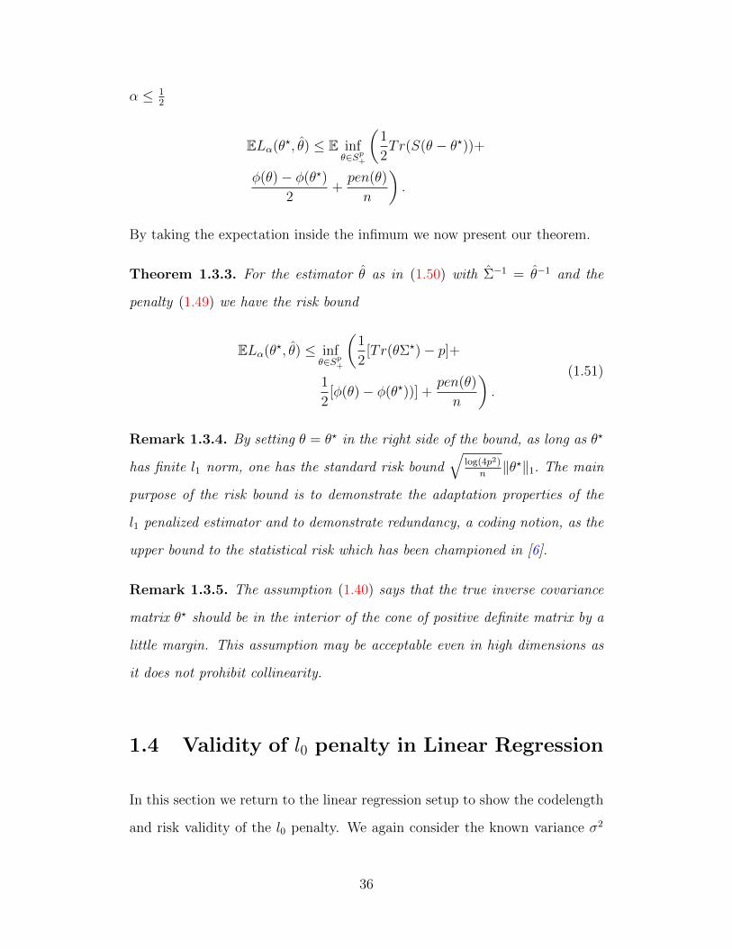
Theorem 1.3.3. For the estimator θ as in (1.50) with Σ−1 = θ−1 and the

penalty (1.49) we have the risk bound

ELα(θ?, θ) ≤ infθ∈Sp+

(1

2[Tr(θΣ?)− p]+

1

2[φ(θ)− φ(θ?))] +

pen(θ)

n

).

(1.51)

Remark 1.3.4. By setting θ = θ? in the right side of the bound, as long as θ?

has finite l1 norm, one has the standard risk bound√

log(4p2)n‖θ?‖1. The main

purpose of the risk bound is to demonstrate the adaptation properties of the

l1 penalized estimator and to demonstrate redundancy, a coding notion, as the

upper bound to the statistical risk which has been championed in [6].

Remark 1.3.5. The assumption (1.40) says that the true inverse covariance

matrix θ? should be in the interior of the cone of positive definite matrix by a

little margin. This assumption may be acceptable even in high dimensions as

it does not prohibit collinearity.

1.4 Validity of l0 penalty in Linear Regression

In this section we return to the linear regression setup to show the codelength

and risk validity of the l0 penalty. We again consider the known variance σ2

36

and the fixed design setup. Our model is

yn×1 = Ψn×pθp×1 + εn×1

where ε ∼ N(0, σ2In×n) and Ψ is the design matrix. The log likelihood of the

model is

− log pθ(y) =1

2σ2‖y −Ψθ‖2

2 +n

2log 2πσ2.

We assume our model is well specified and there is a true vector of coefficients

θ?. Our results would be in the regime when the sample size n is larger than the

number of explanatory variables p. We divide the data y into yin = (yin,Ψin)

consisting of p samples and yf = (yf ,Ψf ) consisting of (n− p) samples. Here

in is intended to suggest initial and f is intended to mean final. It does not

really matter which p samples are chosen to represent the initial sample as

long as it is done once and then remains frozen. We assume that the matrix

Ψin is non singular. The purpose of such division of data is to use the initial

p samples yin to create a Kraft summable penalty on the countable cover we

will choose and then this penalty together with the cover is used to derive

codelength interpretation for the `0 penalized log likelihood or risk bounds for

the estimator minimizing the `0 penalized log likelihood.

1.4.1 Codelength Validity

Ideally one would like a penalty, which is constant on all vectors with a specified

number of non zeroes, to be codelength valid. This cannot be achieved and

the codelength valid penalties have to diverge off to infinity as we go further

out in the parameter space. In an attempt to construct a codelength valid

penalty with the leading term proportional to the `0 norm only, our strategy

37

here is to condition on an initial segment of data. Accordingly let pen(θ|yin)

be a penalty function defined on Θ = Rp which is a function of yin also. So

it is infact a random penalty. The notation is deliberately designed to make

the reader think of pen(θ|yin) as a penalty conditional on the initial data yin.

Analogous to (1.2) we intend to show the existence of a countable set Θ ⊂ Θ

and a Kraft valid codelength V (θ|yin) on Θ such that the following inequality

holds

minθ∈Θ− log pθ(y) + pen(θ|yin) ≥

minθ∈Θ− log pθ(yf ) + V (θ|yin)

(1.52)

where now the right side of (1.52) gives a two stage codelength interpretation

provided we treat it as codelengths on yf conditional on yin and hence the left

side as a function on yf , being not less than the right side, also has a two stage

conditional codelength interpretation. We now proceed to find out a suitable

conditional penalty pen(θ|yin) which would satisfy (1.52).

We introduce some notations and tools which would be used to show both the

codelength validity and the risk validity of a penalty with the main term of

the order k(θ) log n. We now make some relevant definitions and set up some

notations. Let θ ∈ Rp be a given vector. We define k(θ) =∑p

i=1 Iθi 6= 0.

In other words k(θ) is the number of non zeros of the vector θ. We denote

the support of θ or the set of indices where θ is non zero by S(θ). Clearly

|S(θ)| = k(θ). Let S? be the support of the true vector of coefficients θ?. For

any subset S ⊂ [1 : p], let Ψin,S denote the initial part of the design matrix

with column indices in S in natural order. Hence Ψin,S is a p by |S| matrix.

Let us denote the matrix (ΨTin,SΨin,S)−1/2 by MS. We also denote the quantity

1|S|Tr

((ΨT

in,SΨin,S)−1(ΨTf,SΨf,S))

)by ΥS where Tr refers to the trace or sum

38

of diagonals of a matrix.

Let Z denote the set of integers as before. Also fix some δ > 0. For any given

subset S we define a countable set

CS = MSv − w : v ∈ δ(Z − 0)|S| (1.53)

where w is the unique solution to the equation Ψin,Sw = OΨin,Syin. Here OΨin,S

is the orthogonal projection matrix onto the column space of the matrix OΨin,S.

As we have defined, CS is a subset of R|S| but by appending the coordinates

in the complement of S as zeroes, we treat CS as a subset of Rp. We want

to construct Kraft satisfying codelengths and hence subprobabilities on CS

which are proportional to(pφ(yin)

pθ? (yin)

)ηfor any fixed but arbitrary 0 < η ≤ 1.

For that purpose we want to estimate the normalizer which is the quantity∑φ∈CS

(pφ(yin)

pθ? (yin)

)η. The following lemma helps us do exactly that.

Lemma 1.4.1. For all 0 < η ≤ 1 we have

∑φ∈CS

(pφ(yin)

pθ?(yin)

)ηδ|S| ≤ Uη(yin, S) (1.54)

where

Uη(yin, S) = exp(η

2‖OΨin,S∪S?yin −Ψin,S?θ

?‖22

)(2π

η)|S|/2

(1.55)

and OΨin,S∪S? denotes the orthogonal projection matrix onto the column space

of the matrix Ψin,S∪S? .

The proof of this lemma is given in the appendix.

39

We now define the countable set C ⊂ Rp as follows

C = ∪pk=0 ∪S:|S|=k CS. (1.56)

C is the union of the countable sets CS,η over all subsets S ⊂ [1 : p]. Hence

C itself is a countable subset of Rp. By definition, C varies with δ and in

applications we will set δ to be something specific. We now define penalty

functions satisfying Kraft type inequalities on the countable set C. First we

define a family of subprobabilities hη on C as follows

hη(θ, yin) = (1

2)k(θ)+1 1( p

k(θ)

)(pθ(yin)

pθ?(yin))η δk(θ)

1

Uη(yin, S(θ)).

(1.57)

We claim that hη(θ) is a subprobability on Cη for every yin. This can be seen

by first summing hη(θ) over non negative integers k from 0 to p, then summing

over all subsets of [1 : p] with cardinality k and then summing over CS,η. The

inner sum over CS,η of (pθ(yin)pθ? (yin)

)δ|S| 1Uη(yin,S)

is no more than 1 by lemma (1.4.1).

Then for each k we sum over( p

k(θ)

)subsets and the factor 1

( p

k(θ))keeps the overall

sum still no more than 1. Similarly, the factor (12)k(θ)+1 makes the whole sum

less than or equal to 1 when we sum over k from 0 to p, which can be seen by

summing up the geometric series. Hence, we prove our claim.

We can now define Kraft satisfying codelengths lη(θ, yin) on C by defining

lη(θ, yin) = −1

ηlog hη(θ) (1.58)

Then because of hη being a subprobability, it is clear that lη satisfies the

40

following inequality for all yin

∑θ∈C

exp(−ηlη(θ, yin)) ≤ 1. (1.59)

Now we are ready to state our theorem.

Theorem 1.4.2. The penalty pen(θ|yin), defined as below, is conditionally

codelength valid in the sense of (1.52).

pen(θ|yin) =k(θ)

2log(

4n

p) + log

(p

k(θ)

)+

k(θ)

(3 log(2)

2+

log(2π)

2

)+

1

2‖OΨin,S(θ)∪S?yin −Ψin,S?θ

?‖22.

Proof. We declare our countable set Θ = C as defined in (1.56). We also define

V = lη with η = 1 as defined in (1.58). Then we have

V (θ) = (k(θ) + 1) log(2) + log

(p

k(θ)

)+

k(θ) log(1

δ) + log(U(yin, S(θ))− log

pθ(yin)

pθ?(yin).

The task now is to verify (1.52). An equivalent way to verify (1.52) is to verify

the following for any given θ ∈ Θ and data y,

minθ∈Θ− log

pθ(yf )

pθ?(yf )+ log

pθ(y)

pθ?(y)+ V (θ|yin)

≤ pen(θ|yin).

(1.60)

In the case when yin and yf are independent, the log likelihood of the full data

y is the sum of log likelihoods of yin and yf and so we can write the left side

41

of the above equation as

minθ∈Θ− log

pθ(y)

pθ?(y)+ log

pθ(y)

pθ?(y)+(

V (θ|yin) + logpθ(yin)

pθ?(yin)

).

(1.61)

Now our strategy to upper bound the minimum of the above expression is to

restrict the minimum over θ ∈ CS(θ) where CS(θ) is as defined in (1.53). Doing

this cannot decrease the overall minimum because CS(θ) ⊂ Θ by definition of

Θ. Restricted to θ ∈ CS(θ) one can check that the term V (θ|yin) + logpθ(yin)

pθ?(yin)

remains a constant. Now we state a lemma which helps us in upper bound-

ing (1.61).

Lemma 1.4.3.

minθ∈CS(θ)

− logpθ(y)

pθ?(y)+ log

pθ(y)

pθ?(y) ≤ 2(1 + ΥS(θ)) k(θ)δ2. (1.62)

The proof of the above lemma is given in the appendix.

By the above lemma and the fact that V (θ|yin) + logpθ(yin)

pθ?(yin)is constant on

CS(θ),1 we write down the upper bound we get for the left side of (1.61) which

is as follows

2(1 + ΥS(θ)) k(θ)δ2 + (k(θ) + 1) log(2) + log

(p

k(θ)

)+

k(θ) log(1

δ) + log(U(yin, S(θ)).

Setting δ2 = 14(1+ΥS(θ))

we see that a valid penalty satisfying (1.52) would be

pen(θ|yin) =k(θ)

2+ (k(θ) + 1) log(2)+

log

(p

k(θ)

)+k(θ)

2log(4(1 + ΥS(θ))) + log(U(yin, S(θ)).

(1.63)

42

Rearranging and expanding U(yin, S(θ)) we have

pen(θ|yin) =k(θ)

2log(4(1 + ΥS(θ))) + log

(p

k(θ)

)+

k(θ)

(3 log(2)

2+

log(2π)

2

)+

1

2‖OΨin,S(θ)∪S?yin −Ψin,S?θ

?‖22.

With a fixed design matrix there is only one term in the above expression

which is random. It can be checked that the term 12‖OΨin,S∪S?yin −Ψin,S?θ

?‖22

is distributed as a χ2 random variable with degree of freedom at most k(θ)+k?.

So its expected value is going to be at most k(θ) + k?. In the case when the

design matrices Ψin and Ψf have orthogonal columns and the `2 norms of each

of the columns of Ψin and Ψf are atmost p and n−p respectively we then have

for any subset S, ΨTin,SΨin,S = pI|S|×|S| and ΨT

f,SΨf,S = (n− p)I|S|×|S|. In that

case it can be checked that γS = n−pp. Hence in this situation, our codelength

valid penalty conditional on yin becomes exactly as defined in Theorem (1.68).

This completes the proof of Theorem (1.68).

Remark 1.4.1. Note that the leading term of the expected penalty pen(θ|yin)

is indeed going to be the traditional log(n))2

k(θ) in case p does not grow with

n. In case p grows as nβ for some 0 < β < 1 then the leading term of of

the expected penalty pen(θ|yin) is still some constant times k(θ) log(n). We

remind the reader that k(θ) log(p/k(θ)) ≤ log((p

k(θ)

)) ≤ k(θ) log(ep/k(θ)). So

the term log((p

k(θ)

)) again contributes a constant times k(θ) log(n) term in case

p is growing as some power of n.

43

1.4.2 Risk validity

In this section we show the risk validity of the l0 penalty by leveraging its

codelength interpretation as shown in the last subsection. To prove risk bounds

by the same reasoning as in section (1.2.2) we need to adapt the arguments in

section (1.2.2) to the case when we have data split into two parts. We define

our family of loss functions between two probability distributions p and q on

X n in the same way as before except that it only depends on the final part of

the data Xf . Let 0 < α ≤ 1 be a fixed, arbitrary number. We define our loss

function as follows

Lα(p, q) = − 1

αlog(E(

q(yf )

p(yf ))α). (1.64)

Also for a penalty pen(θ|yin) depending on yin we define our penalized likeli-

hood estimator to be

θ(y) = argminθ∈Θ

− log pθ(y) + pen(θ|yin). (1.65)

We now present the theorem which will help us in proving risk bounds for

the `0 penalized likelihood estimator. Fix 0 < α < 1. For our countable set

Θ = C and codelengths V = lα as defined in (1.58), clearly the following is

true by (1.59). ∑θ∈Θ

exp(−αV (θ|yin)) ≤ 1. (1.66)

We expand V to get

V (θ|yin) =1

α

((k(θ) + 1) log(2) + log

(p

k(θ)

)+

k(θ) log(1

δ) + log(Uα(yin, S(θ))

)− log

pθ(yin)

pθ?(yin)

.

44

We would like to now verify the following

minθ∈Θ− log

pθ(yf )

pθ?(yf )+ log

pθ(y)

pθ?(y)+

Lα(pθ? , pθ)− Lα(pθ? , pθ) + V (θ|yin) ≤ pen(θ).

(1.67)

Verifying the above gives us risk bounds as is shown in the following lemma.

Lemma 1.4.4. Assuming the existence of a countable subset Θ ⊂ Θ and a

penalty function V (.|yin) defined on F satisfying (1.66) and (1.67), we have

the following risk bound

ELα(pθ? , pθ) ≤ Eminθ∈Θ

(log

pθ?(y)

pθ(y)+ pen(θ|yin)

).

The proof of this lemma parallels the proof of Theorem (1.2.3) and is given in

the appendix.

Now we proceed to verify (1.66) in order to derive the risk bound in theo-

rem (1.4.4) for the l0 penalized estimator in the linear regression setting. We

can write the left side in (1.67) as

minθ∈Θ− log

pθ(y)

pθ?(y)+ log

pθ(y)

pθ?(y)+ Lα(pθ? , pθ)−

Lα(pθ? , pθ) +

(Vα(θ|yin) + log

pθ(yin)

pθ?(yin)

).

Again we upper bound the minimum of the above expression by restricting to

θ ∈ CS(θ) which cannot decrease the overall minimum. Restricted to θ ∈ CS(θ)

it turns out that the term Vα(θ|yin) + logpθ(yin)

pθ?(yin)remains a constant. The

following lemma now helps us.

45

Lemma 1.4.5. Given any θ and data y we have the following inequality

minθ∈CS(θ)

(log(

pθ(y)

pθ(y)) + Lα(pθ, pθ?)− Lα(pθ, pθ?)

)≤ 2k(θ)δ2(1 + αΥS(θ))

Hence we get an upper bound for the left side of (1.67) which is as follows

2k(θ)δ2(1 + αΥS(θ)) +(k(θ) + 1) log(2)

α+

log(p

k(θ)

)α

+k(θ)

αlog(

1

δ) +

log(U(yin, S(θ))

α.

Setting

δ2 =1

4α(1 + αΥS(θ))

we see that a risk valid penalty would be

penα(θ|yin) =

k(θ)

2αlog(4α(1 + αΥS(θ))) +

k(θ)

2α+

(k(θ) + 1) log(2)

α+

log(p

k(θ)

)α

+log(Uα(yin, S(θ))

α.

Rearranging and expanding logUα(yin, S(θ)) we have

penα(θ|yin) =

k(θ)

2αlog(4α(1 + αΥS(θ))) + αΨT

f Ψf ))+

(k(θ) + 1) log(2)

α+

log(p

k(θ)

)α

+k(θ)

2log(

2π

α)+

1

2‖OΨin,S∪S?yin −Ψin,S?θ

?‖22.

(1.68)

By taking the expectation inside the minimum in the right side and then doing

some algebraic manipulations of the statement of Theorem (1.4.4), we get the

46

resolvability risk bound which we write down below as a theorem.

Theorem 1.4.6. With the estimator being defined as in (1.65) and penα(θ|yin)

as defined in (1.68) we have the risk bound for all 0 < α ≤ 1,

E1

2n‖yf (θ − θ?)‖2

2 ≤1− ασ2

infθ∈Rp

(1

2n‖yf (θ − θ?)‖2

2 +1

nEin pen(θ|yin)

).

Remark 1.4.2. As we can see, as α is taken to be near zero, the constant

outside the right side in theorem (1.4.6) approaches the desired value 1. But

then we have to pay for the fact that the penalty contains terms divided by α

which blow up when α is brought near zero.

By setting θ = θ? inside the infimum in the above theorem we obtain

E1

2n‖yf (θ − θ?)‖2

2 ≤1− ασ2

Einpen(θ?|yin)

n. (1.69)

Remark 1.4.3. The random part depending on yin in pen(θ?|yin) is

‖OΨin,S∪S?yin −Ψin,S?θ?‖2

2.

The above term is distributed as a χ2 random variable with degrees of freedom

at most k(θ) + k(θ?). In the case when the design matrices Ψin and Ψf are

orthogonal and the `2 norms of the columns of Ψin and Ψf are atmost p and

n−p respectively we then have ΥS = n−pp. Then the leading term of the expected

penalty is of the order k(θ) log(n) and hence we atleast have a k(θ?) log(n)/n

rate of convergence of the left side in (1.69).

Remark 1.4.4. Our risk bounds are useful even when p grows like a constant

fraction of n.

47

1.5 Conclusion

We have contributed to a general theory of penalized likelihood estimation

by building a connection to two stage coding procedures in MDL, even in

uncountable parameter spaces. For a given penalty, we have proposed that ex-

istence of appropriate countable covers of the parameter space imply adaptive

statistical risk bounds for the penalized likelihood estimator on any model as

long as data is being generated in an i.i.d fashion. We then have exhibited

multiple ways as to how to construct these countable covers and verify the

needed properties in certain canonical problems in statistics.

1.6 Appendix

1.6.1 Proof of Lemma (1.3.1)

We are to show∑

z∈Zp exp(−C(z)) ≤ 1 where

C(z) = |z|1 log(p+ 1) + 2.

Proof. It can be easily checked by summing up the geometric series that

∑z∈Z

(1

p+ 1)|z| = 1 +

2

p.

Hence we have ∑z∈Zp

(1

p+ 1)|z|1 = (1 +

2

p)p.

48

We can divide by (1 + 2p)p both sides and exponentiate to get

∑z∈Zp

exp

(−|z|1 log(p+ 1)− p log(1 +

2

p)

)≤ 1.

Using the fact that p log(1 + 2p) ≤ 2 we have

∑z∈Zp

exp (−|z|1 log(p+ 1)− 2) ≤ 1.

Recalling the definition of C(z) this completes the proof of Lemma (1.3.1).

Sampling method 2 for linear regression

Here we show an alternative method for demonstrating an upper bound to the

sum of discrepancies plus complexity term in the linear regression case. Θ and

V are defined as in (1.25) and (1.26) respectively. Let θ be any given vector

in Rp and let us first consider the quadratic term which is the following

α

2σ2

n∑i=1

(fθ(xi)− fθ(xi))2.

By expanding out fθ and fθ in terms of the dictionary functions the last display

becomes

α

2σ2

n∑i=1

(

p∑j=1

(θj − θj)fj(xi))2. (1.70)

Let δ be a positive real number. Let K(θ) = d |θ|w,1δe. K(θ) is the least integer

larger than or equal to |θ|w,1 divided by δ. We will write K = K(θ) to minimize

notational clutter. In order to explain our sampling strategy, we first define a

random variable h. Let ejpj=1 denote the canonical basis of Rp. The random

vector h takes value Kδsign(θj)ejwj

with probabilitywjθjKδ

for all j = 1, . . . , p.

With the remaining probability, h takes the form of the zero vector. One

49

can check that h defined this way is unbiased for θ, that is E(h1) = θ. Say

we sample K i.i.d copies h1, . . . , hk. of h. We now consider the mean of these

random vectors h = 1K

∑Ki=1 hi. We denote the distribution of h by µ. Clearly,

h is also unbiased for θ. We first note that

Eµ(

p∑j=1

((hj − θj)fj(xi))2 =1

KEh(

p∑j=1

((hj − θj)fj(xi))2.

This is because h is the sum of K i.i.d copies of h and h is unbiased for θ. Now

we can upper bound the expectation over hlKl=1 of the above term as follows

Eh(p∑j=1

((hj − θj)fj(xi))2 ≤ Eh(p∑j=1

hjfj(xi))2.

The above inequality follows due to unbiasedness of h1 and by the simple fact

that the variance of any random variable is at most the expected square of that

random variable. We note the fact that for any j 6= l the cross product terms

hjhl = 0 pointwise by definition of h. Now summing over i and combining the

previous two inequalities we obtain the following result

Eµn∑i=1

(

p∑j=1

(hj − θj)fj(xi))2 ≤ n

K

p∑j=1

w2jEh(hj)

2. (1.71)

For any j we also have by definition of the random variable h

Ehh2j =

Kδθjwj

. (1.72)

So combining the last two equations we have

Eµn∑i=1

(

p∑j=1

(hj − θj)fj(xi))2 ≤ nδ|θ|w,1. (1.73)

50

Now we consider the penalty or the complexity term. We note that each

coordinate of h has a fixed sign depending on the signs of the coordinates of

θ. Therefore, linearity of expectation extends to absolute values also, in other

words it can be checked that the following holds for any j ∈ [1 : p]

Eµ|hj| = E|hj|

The above equation and the definition of V implies the following fact

EµV (h) = EhV (h).

It is clear now from the definition of h and the definition of V the following

holds

EµV (h) =K log(p+ 1) + 2

α.

So by the above arguments we can conclude that Hθ on an average is upper

bounded by the following expression

α

2σ2nδ|θ|w,1 +

K log(p+ 1) + 2

α.

Using the fact that K ≤ |θ|w,1δ

+ 1 we have the expression in the last display

can be further upper bounded by the following expression

α

2σ2nδ|θ|w,1 +

|θ|w,1δ

log(p+ 1)

α+

log(p+ 1) + 2

α.

Setting δ2 = 2σ2 log(p+1)α2n

we obtain the following that by defining the penalty

function on Θ as follows

pen(θ) =1

σ

√2n log(4p)|θ|w,1 +

log(p+ 1) + 2

α. (1.74)

51

we define a risk valid penalty.

Remark 1.6.1. Comparing the penalties in (1.37) and (1.74) we see that (1.74)

contains an extra log(p+1)α

term. In this sense (1.37) is an improvement over (1.37)

which was obtained in the linear regression problem in [3].

This completes this subsection.

1.6.2 Proof of Lemma (1.4.1)

Proof. We fix any subset S ⊂ [1 : p]. We first relate the sum over φ ∈ CS of

the following expression

(Pφ(yin)

Pθ?(yin))ηδ|S|

to the integral of the same expression over all of R|S|. By Pythagorus theorem,

we have

‖yin −Ψin,Sφ‖22 =

‖yin −OΨin,Syin‖22 + ‖OΨin,Syin −Ψin,Sφ‖2

2

where OΨin,S denotes the orthogonal projection matrix to the column space of

the matrix Ψin,S. Hence one can check

(Pφ(yin)

Pθ?(yin))η = A

∑φ∈CS

exp(−η

2‖OΨin,Syin −Ψin,Sφ‖2

2

)(1.75)

where

A = exp(−η

2‖yin −OΨin,Syin‖2

2 + ‖yin −Ψin,S?θ?‖2

2). (1.76)

52

Note that by properties of orthogonal projections,

‖yin − yin,S?θ?‖22 − ‖yin −Oyin,Syin‖2

2 ≤

‖yin − yin,S?θ?‖22 − ‖yin −Oyin,S∪S?yin‖

22 =

‖Oyin,S∪S?yin − yin,S?θ?‖2

2.

Hence we have

A ≤ exp(−η2‖Oyin,S∪S?yin − yin,S?θ

?‖22). (1.77)

Now we can always write OΨin,Syin = Ψin,Sw for some vector w because

OΨin,Syin lies in the column space of OΨin,Syin. So we have

∑φ∈CS

exp(−η

2‖OΨin,Syin −Ψin,Sφ‖2

2

)=

∑φ∈CS

exp(−η

2(φ− w)TΨT

in,SΨin,S(φ− w)) (1.78)

Now recalling the definition of CS = MSv − w : v ∈ G |S| where w is the

unique solution to the equation Ψin,Sw = OΨin,Syin we can change variables

and express the sum over CS now as a sum over G |S| as follows:

∑φ∈CS

exp(−η2

(φ− w)TΨTin,SΨin,S(φ− w) =

∑v∈G|S|

exp(−η2vTv).

(1.79)

Now the right side in the above equation appears while constructing an appro-

priate lower Reimann sum to an integral as we argue now. Imagine dividing

up R|S| into cubes of sidelength δ with the vertices of the cubes constiting the

set δZp. In order to minimize exp(−η2vTv) for v in a cube, it is clear that one

should choose v so that the absolute value of each of its coordinate is maxi-

53

mized. This implies that as we run over all the cubes, the minimizing points

would be precisely the set G |S|. Since we are picking out the minimizing points

and the volume of the cubes is δ|S| we have

∑v∈G|S|

exp(−η2vTv)δ|S| ≤

∫R|S|

exp(−η2vTv)dv. (1.80)

The above equation just states that the lower Reimann sum is upper bounded

by the integral. Now it can be checked that∫R|S| exp(−η

2vTv)dv = (2π/η)|S|/2.

Hence by (3.12) we have

A

∫R|S|

exp(−η2vTv)dv ≤ Uη(yin,S) (1.81)

where we recall that

Uη(yin,S) = exp(η

2‖OΨin,S∪S?yin −Ψin,S?θ

?‖22

)(2π

η)|S|/2.

So then by combining all the above equations (3.11), (3.12), (1.78), (1.79), (1.80), (1.81)

we have the desired inequality

∑φ∈CS

(pφ(yin)

pθ?(yin))ηδ|S| ≤ Uη(yin, S).

This completes the proof of Lemma (1.4.1).

1.6.3 Proof of Lemma (1.4.3)

Proof. For all θ ∈ CS(θ) clearly k(θ) ≤ k(θ) by definition of CS(θ) as all the

coordinates in the complement of S are set to zero. In this subsection when

we write vectors θ ∈ CS(θ),α and θ, we really mean θS(θ) and θS(θ) which are

54

|S| dimensional vectors. We do not burden the notation here by adding extra

subscripts. Now if we expand the log likelihoods we obtain

logpθ(y)

pθ(y)=

1

2σ2‖y −ΨS θ‖2

2 −1

2σ2‖y −ΨSθ‖2

2. (1.82)

After simplifications and noting ΨTΨ = ΨTinΨin + ΨT

f Ψf we see that we have

to upper bound the following expression

minθ∈CS(θ)

1

2σ2‖Ψin,S θ −Ψin,Sθ‖2

2 +1

2σ2‖Ψf,S θ −Ψf,Sθ‖2

2

+ l(θ − θ)

where l is an affine function. Setting θ = MS v − w and θ = MSv − w where

v = (MS)−1(θ + w) we have that the expression in the last display equals

minv∈G|S|

1

2σ2(v − v)T (v − v) +

1

2σ2(v − v)TB(v − v)

+ l(MS v −MSv)

where the matrix B equals MSΨTf,SΨf,SMS. Now our strategy is to upper

bound the above minimum by an expectation with respect to a carefully chosen

distribution. We now describe the choice of the distribution. Consider v =

(v1, . . . , vS(θ)). For each coordinate l, one can devise a distribution taking only

two values in Z − 0 such that the expectation of this distribution is vl. The

two values are namely the smallest non zero integer not lesser than vl and the

largest non zero integer not bigger than vl. Hence one can devise a distribution

on G |S| with the property that each coordinate of the random vector drawn

from two valued distributions as described is independent and the average of

this distribution is the vector v. Now since we are only choosing points from

closeby cubes any coordinate of v − v is atmost 2δ in absolute value with

55

probability 1. For any quadratic form (v − v)TQ(v − v) where Q is some non

negative definite matrix, by unbiasedness and independence of the coordinates,

its expectation boils down to the expectation of the diagonal terms. Therefore

we have

E(v − v)TQ(v − v) = (2δ)2Tr(Q).

Also, l being an affine function of v− v is zero on an average. So applying the

above facts we have the following inequality

E1

2‖Ψinθ −Ψinθ‖2

2 + E1

2‖Ψf θ −Ψfθ‖2

2+

El(θ − θ) ≤ 2δ2(k(θ) + Tr(B)).

(1.83)

Now by definition of ΥS(θ), we have

2δ2(k(θ) + Tr(B)) = 2δ2k(θ)(1 + ΥS(θ)).

Hence we get the desired bound

minθ∈CS(θ)

logpθ(y)

pθ(y)≤ 2(1 + ΥS(θ))k(θ)δ2. (1.84)

This completes the proof of Lemma (1.4.3). The proof of Lemma (1.4.5) goes

along very similar lines to this proof and hence is left to the reader.

56

1.6.4 Proof of Lemma (1.4.4)

Proof. By the definition of θ we have

Lα(pθ? , pθ) =(Lα(pθ? , pθ)− log

pθ?(y)

pθ(y)− pen(θ)

)+

minθ∈Θ

(log

pθ?(y)

pθ(y)+ pen(θ)

).

(1.85)

The exponential of the first term in the brackets in the above display can be

upper bounded as follows.

exp

(αLα(pθ? , pθ)− log

pθ?(y)

pθ(y)− pen(θ|yin)

)≤∑

θ∈Θ

exp(αLα(pθ? , pθ))(pθ(yf )

p(yf ))α

exp(−αV (θ|yin)).(1.86)

This follows by (1.66) and non negativity of the exponential function. We can

now take expectation with respect to yf conditional on yin. The right side of

the last display then becomes

∑θ∈Θ

exp(αLα(pθ? , pθ))Ef (pθ(yf )

p(yf ))α

exp(−αV (θ|yin)).

By the definition of the loss function Lα and the summability condition on V

for every yin as in (1.67), the above expression is not greater than 1 and hence

the expectation of the left side in (1.86) too is not greater than 1. Now by

concavity of the logarithm and Jensen’s inequality we obtain

Ef log

(exp(αLα(pθ? , pθ))(

pθ(y)

pθ?(y))α

exp(−α pen(θ|yin))≤ 0.

(1.87)

57

The above is just α times the first term in brackets in (1.85). Hence from (1.85)

and (1.87) we get an upper bound of the expected loss function conditional on

yin where expectation is taken over yf ,

EfL(pθ? , pθ) ≤ Ef minθ∈Θ

(log

pθ?(y)

pθ(y)+ pen(θ|yin)

).

Now by taking expectation with respect to yin we obtain the following risk

bound, where E refers to expectation taken over the whole data,

ELα(pθ? , pθ) ≤ Eminθ∈Θ

(log

pθ?(y)

pθ(y)+ pen(θ|yin)

).

This completes the proof of Lemma (1.4.4).

58

Bibliography

[1] A.R. Barron and T.M. Cover, “Minimum complexity density estima-

tion,” IEEE Trans. Inform. Theory. Vol.37, No.4, pp.1034–1054. 1991.

[2] A.R. Barron, C. Huang, J.Q. Li, X. Luo, “The MDL principle, penal-

ized likelihoods, and statistical risk,” In Festschrift for Jorma Rissanen.

Tampere University Press, Tampere, Finland, 2008.

[3] A.R. Barron, C. Huang, J.Q. Li, X. Luo, “MDL, penalized likelihood

and statistical risk,” IEEE Information Theory Workshop. Porto Por-

tugal, May 4-9, 2008.

[4] A.R. Barron, J. Rissanen, and B. Yu, “The minimum description length

principle in coding and modeling,” IEEE Trans. Inform. Theory.

Vol.44, No.6, pp.2743–2760. 1998. Special Commemorative Issue: In-

formation Theory: 1948-1998.

[5] A. Bhattacharyya, “On a measure of divergence between two statistical

populations defined by probability distributions,” Bull. Calcutta Math.

Soc. Vol.35, pp.99–109. 1943.

[6] P. Grunwald, The Minimum Description Length Principle. Cambridge,

MA, MIT Press. 2007.

[7] P. Buhlmann S. Van De Geer, “Statistics for high-dimensional data.

59

Methods, theory and applications,” Springer Series in Statistics.

Springer, Heidelberg.

[8] J. Rissanen (2004), “An introduction to the MDL principle,” Available

at www.mdl-research.org.

[9] A. R. Barron, “Complexity Regularization with application to artificial

neural networks,” “Nonparametric Functional Estimation and Related

Topics,” G. Roussas (Ed.) pp. 561-576. Dordrecht, the Netherlands:

Kluwer Academic Publishers.

[10] A. R. Barron, L. Birge, P. Massart, “Risk bounds for model selection

by penalization,” Probability Theory and Related Fields, 1999 Volume

113, pp. 301-413.

[11] L. Birge and P. Massart, “Rates of convergence for minimum contrast

estimator,” Probability Theory and Related Fields 1998 Volume 97,

113-150.

[12] L. Birge and P. Massart, “Minimum contrast estimators on sieves: ex-

ponential bounds and rates of convergence,” Bernoulli 1998 Volume 4,

329-375.

[13] F. Cucker, and S. Smale, On the mathematical foundations of learning.

Bulletin of the American Mathematics Society 2001 Volume 39. pp. 1-

49.

[14] D. D. Cox, F. O’Sullivan, “Asymptotic analysis of penalized likelihood

and related estimators,” Annals of Statistics, 1990 Volume 18, pp. 1676-

1695.

60

[15] G. M. de Montricher, R. Tapia and J. R. Thompson, “Nonparamet-

ric maximum likelihood estimation of probability densities by penalty

function methods,” Annals of Statistics 1975 Volume 3, pp. 1329-1348

[16] E. D. Kolaczyk, R. D. Nowak, “Multiscale likelihood analysis and com-

plexity penalized estimation,” Annals of Statistics 2004 Volume 32, pp.

500-527.

[17] E. D. Kolaczyk, R. D. Nowak, “Multiscale generalized linear models for

nonparametric function estimation,” Biometrika 2005 Volume 92, No.

1, pp. 119-133.

[18] J. Q. Li, “Estimation of Mixture Models,” Ph.D. Thesis, 1999, Depart-

ment of Statistics, Yale University, New Haven, CT.

[19] A. S. Nemirovskii, B. T. Polyak, A. B. Tsybakov, “Rate of convergence

of nonparametric estimates of maximum likelihood type,” Problems in

Information Transmission 1985 Volume 21, pp. 258-272.

[20] X. Shen, “On the method of Penalization,” Statistica Sinica, 1998 Vol-

ume 8, pp. 337-357.

[21] B. Silverman, “On the estimation of probability function by the max-

imum penalized likelihood method,” Annals of Statistics 1982 Volume

10, 795-810.

[22] R. A. Tapia, J. R. Thompson, “Nonparametric Probability Density Es-

timation,” Baltimore, MD: The Johns Hopkins University Press 1978.

[23] G. Wahba, “Spline Models for Observational Data,” Philadelphia, PA:

SIAM 1990.

61

[24] Y. Yang and A. R. Barron, “An asymptotic property of model selection

criteria,” IEEE Transactions on Information Theory, 1998, Volume 44,

pp. 117-133.

[25] Y. Yang and A. R. Barron, “Information-theoretic determination of

minimax rates of convergence,” Annals of Statistics, 1999 Volume 27,

pp. 1564-1599.

[26] S. Negahban, P. Ravikumar, M. J. Wainwright, B. Yu, “A Unified

Framework for High-Dimensional Analysis of M-Estimators with De-

composable Regularizers,” Statistical Science 27 (2012), no. 4, 538–557.

doi:10.1214/12-STS400. http://projecteuclid.org/euclid.ss/1356098555.

[27] F. Bunea, A. Tsybakov, M. Wegkamp, “Aggregation for Gaussian

regression,” The Annals of Statistics 35 (2007), no. 4, 1674–1697

http://projecteuclid.org/euclid.aos/1188405626.

62

Chapter 2

Improved Risk Bounds in

Monotone Regression and other

Shape Constraints

We consider the problem of estimating an unknown non-decreasing sequence

θ ∈ Rn from a noisy observation. We give an improved global risk upper

bound for the isotonic least squares estimator (LSE) in this problem. The

obtained risk bound behaves differently depending on the form of the true

sequence θ – one gets a whole range of rates from log n/n (when θ is constant)

to n−2/3 (when θ is uniformly increasing in a certain sense). In particular,

when θ has k constant pieces then the risk bound becomes (k/n) log(en/k).

As a consequence, we illustrate the automatic adaptation properties of the

LSE. We also derive local minimax lower bounds for this problem which show

that the LSE is nearly optimal in a local non-asymptotic minimax sense. We

prove an analogue of our risk bound for model misspecification where the true

θ is not necessarily non-decreasing. We also derive global risk upper bounds

63

for the LSE of θ when θ belongs to a known but arbitrary convex polyhedral

cone in Rn.

2.1 Introduction

Consider the problem of estimating an unknown non-decreasing regression

function f0 from finitely many noisy observations. Specifically, only under the

assumption that f0 is non-decreasing, the goal is to estimate f0 from data

(x1, Y1), . . . , (xn, Yn) with

Yi = f0(xi) + εi, for i = 1, 2, . . . , n, (2.1)

where ε1, . . . , εn are i.i.d mean zero errors with variance σ2 > 0 and x1 < · · · <

xn are fixed design points. This is one of the canonical problems in the area

of shape-constrained nonparametric function estimation.

The most natural and commonly used estimator for this problem is the mono-

tone least squares estimator (LSE), proposed in [6] and [2]; also see [16] for the

related problem of estimating a non-increasing density. The LSE is defined as

any minimizer of the LS criterion:

fls ∈ argming∈C

n∑i=1

(Yi − g(xi))2 (2.2)

where C denotes the set of all real-valued non-decreasing functions on R. The

values fls(x1), . . . , fls(xn) are unique and can be computed easily using the

pool adjacent violators algorithm; see [26, Chapter 1].

The existing theoretical results on monotone function estimation can be grouped

into two categories: (1) results on the behavior of the LSE at an interior point

64

(which is sometimes known as local behavior), and (2) results on the behavior

of a global loss function measuring how far fls is from f0. Before describing

our results, let us briefly review the results on the local behavior of the LSE.

The results on the behavior of the LSE under a global loss function will be

detailed while describing our main results.

Results on the local behavior are proved, among others, in [7], [19], [17], [9],

[10], and [22]. Under certain regularity conditions on the unknown function f0

near the interior point x0, [7] showed that fls(x0) converges to f0(x0) at the rate

n−1/3 and also characterized the limiting distribution of n1/3(fls(x0)− f0(x0)).

In the related (non-increasing) density estimation problem, [17], [9] and [22]

showed that if the interior point x0 lies on a flat stretch of the underlying

function then the LSE (which is also the nonparametric maximum likelihood

estimator, usually known as the Grenander estimator) converges to a non-

degenerate limit at rate n−1/2, and they characterized the limiting distribu-

tion. [10] showed that the rate of convergence of fls(x0) to f0(x0) depends on

the local behavior of f0 near x0 and explicitly described this rate for each f0.

In this sense, the LSE fls adapts automatically to the unknown function f0.

[10] also proved optimality of the LSE for local behavior by proving a local

asymptotic minimax lower bound.

Often in monotone regression, the interest is in the estimation of the entire

function f0 as opposed to just its value at one fixed point. In this sense, it

is more appropriate to study the behavior of fls under a global loss function.

The most natural and commonly studied global loss function in this setup is

`2(f, g) :=1

n

n∑i=1

(f(xi)− g(xi))2

for real valued functions f and g. Note that under this loss function, the prob-

65

lem posited in (2.1) becomes a vector or sequence estimation problem where

the goal is to estimate the vector θ := (θ1, . . . , θn) ∈ Rn from observations

Yi = θi + εi, for i = 1, 2, . . . , n, (2.3)

under the constraint that the unknown sequence θ = (θ1, . . . , θn) satisfies

θ1 ≤ · · · ≤ θn. In other words, we assume that θ lies in the closed convex

polyhedral cone M defined as

M := t ∈ Rn : t1 ≤ t2 ≤ · · · ≤ tn.

The connection between this sequence estimation problem and the earlier prob-

lem of monotone regression is apparent by the identification θi = f0(xi). As

a result, it is obvious that the exact form of the design points x1, . . . , xn is

irrelevant in the problem (2.1) as long as x1 < · · · < xn.

Henceforth we would be stating our results for sequences although they could

be thought of as being generated from a monotone function sampled at certain

design points. The LSE, θ, of θ is defined as

θ := argmint∈M

n∑i=1

(Yi − ti)2 (2.4)

and it is easy to see that it exists and is unique. We study the risk of θ under

the loss function∑n

i=1(ti−si)2/n which we denote by `2(t, s) by a slight abuse

of notation.

The behavior of the LSE θ, under the loss `2, has been studied in a num-

ber of papers including [30, 31], [12], [4], [34], [23] and [35]. If one looks at

the related (non-increasing) density estimation problem, [5] developed non-

66

asymptotic risk bounds for the Grenander estimator, measured with the L1-

loss, whereas [31] has results on the Hellinger distance.

The strongest results on the behavior of the LSE θ, under the loss `2, are

obtained by [35] who proved non-asymptotic bounds on the risk Eθ`2(θ, θ)

under a minimal set of assumptions on the errors ε1, . . . , εn. Among other

things, [35, Theorem 2.2] showed that

Eθ`2(θ, θ) . RZ(n; θ) (2.5)

where

RZ(n; θ) :=

(σ2V (θ)

n

)2/3

+σ2 log n

n.

with

V (θ) := θn − θ1.

Here, by the symbol . we mean ≤ up to a multiplicative constant. The

quantity V (θ) is the variation of the sequence θ. When V (θ) = 0, i.e., when θ

is a constant sequence, this inequality implies that

Eθ`2(θ, θ) .σ2 log n

n. (2.6)

This result is an example of the adaptation behavior of the LSE in the sense

that the risk bound when θ is constant is much smaller than the general upper

bound (2.5). The rate log n/n also appears in the risk bound for the Grenander

estimator when the underlying function is constant; see [20], [19] and [31]. In

fact, it has been shown that in this case, the integrated squared error risk,

properly normalized, converges to a normal distribution. Other results on the

global behavior of the LSE can be found in [13, 14] who considered a different

global loss function and characterized the limiting distribution of a suitably

67

normalized version.

An important shortcoming of the risk bound (2.5) is that it is not optimal

in the sense that the risk Eθ`2(θ, θ) can, in general, be much smaller than

RZ(n; θ). The main result of this paper presents an improvement of (2.5).

To describe our result, let us introduce some notation. We say an interval

partition π of a positive integer n is a finite sequence of positive integers that

sum to n. In combinatorics this is called a composition of n. Let the set of all

interval partitions π of n be denoted by Π. Formally, Π can be written as

Π :=

(n1, n2, .., nk) : k ≥ 1, ni ∈ N and

k∑i=1

ni = n

.

For each π ∈ Π, let k(π) denote the length of the associated sequence ni.

For each θ = (θ1, . . . , θn) ∈M, there exist integers k and n1, . . . , nk with ni ≥ 1

and n1 + · · ·+nk = n such that θ is constant on each set j : si−1 +1 ≤ j ≤ si

for i = 1, . . . , k, where s0 := 0 and si = n1 + · · ·+ ni. We refer to the interval

partition πθ := (n1, . . . , nk) as the interval partition generated by θ. By a slight

abuse of notation, we denote k(πθ) by simply k(θ). Note that k(θ) is just the

number of distinct values among θ1, . . . , θn. k(θ) is a measure of sparsity of

the differences θi − θi−1 for i = 2, . . . , n.

For every θ ∈M and π := (n1, . . . , nk) ∈ Π, we define

Vπ(θ) = max1≤i≤k

(θsi − θsi−1+1

).

where s0 := 0 and si = n1 + · · · + ni for 1 ≤ i ≤ k. Vπ(θ) can be treated

as measure of variation of θ with respect to the partition π. An important

property is that Vπθ(θ) = 0 for every θ ∈M. For the trivial partition π = (n),

it is easy to see that Vπ(θ) = V (θ).

68

We are now ready to state our main result. In Theorem 2.2.1, we prove the

following non-asymptotic risk bound:

Eθ`2(θ, θ) ≤ R(n; θ) (2.7)

where

R(n; θ) := 4 infπ∈Π

(V 2π (θ) +

4σ2k(π)

nlog

en

k(π)

). (2.8)

Let us explain why our bound (2.7) is an improvement of (2.5) in certain

cases. Suppose, for example, θj = Ij > n/2 (here I denotes the indicator

function) and hence V (θ) = 1. Then RZ(n; θ) is essentially (σ2/n)2/3 while

R(n; θ) is much smaller because it is at most (32σ2/n) log(en/2) as can be

seen by taking π = πθ in (2.8).

More generally by taking π = πθ in the infimum of the definition of R(n; θ),

we obtain

Eθ`2(θ, θ) ≤ 16k(θ)σ2

nlog

en

k(θ), (2.9)

which is a stronger bound than (2.5) when k(θ) is small. The reader may

observe that k(θ) is small precisely when the differences θi − θi−1 are sparse.

We prove some properties of our risk bound R(n; θ) in Section 2.3. In The-

orem 2.3.1, we show that R(n; θ) is bounded from above by a multiple of

RZ(n; θ) that is at most logarithmic in n. Therefore, our inequality (2.7) is

always only slightly worse off than (2.5) while being much better in the case of

certain sequences θ. We also show in Section 2.3 that the risk bound R(n; θ)

behaves differently depending on the form of the true sequence θ. This means

that the bound (2.7) demonstrates adaptive behavior of the LSE. One gets

a whole range of rates from (log n)/n (when θ is constant) to n−2/3 up to

logarithmic factors in the worst case (this worst case rate corresponds to the

69

situation where mini(θi − θi−1) & 1/n). The bound (2.7) therefore presents a

bridge between the two terms in the bound (2.5).

In addition to being an upper bound for the risk of the LSE, we believe that

the quantity R(n; θ) also acts as a benchmark for the risk of any estimator in

monotone regression. By this, we mean that, in a certain sense, no estimator

can have risk that is significantly better than R(n; θ). We substantiate this

claim in Section 2.4 by proving lower bounds for the local minimax risk near

the “true” θ. For θ ∈M, the quantity

Rn(θ) := inft

supt∈N(θ)

Et`2(t, t)

with

N(θ) :=t ∈M : `2

∞(t, θ) . R(n; θ)

will be called the local minimax risk at θ (see Section 2.4 for the rigorous

definition of the neighborhood N(θ) where the multiplicative constants hidden

by the . sign are explicitly given). In the above display `∞ is defined as

`∞(t, θ) := maxi |ti − θi|. The infimum here is over all possible estimators t.

Rn(θ) represents the smallest possible (supremum) risk under the knowledge

that the true sequence t lies in the neighborhood N(θ). It provides a measure

of the difficulty of estimation of θ. Note that the size of the neighborhood

N(θ) changes with θ (and with n) and also reflects the difficulty level of the

problem.

Under each of two following setups for θ, and the assumption of normality

of the errors, we show that Rn(θ) is bounded from below by R(n; θ) up to

multiplicative logarithmic factors of n. Specifically,

1. when the increments of θ (defined as θi− θi−1, for i = 2, . . . , n) grow like

70

1/n, we prove in Theorem 2.4.3 that

Rn(θ) &

(σ2V (θ)

n

)2/3

&R(n; θ)

log(4n); (2.10)

2. when k(θ) = k and the k values of θ are sufficiently well-separated, we

show in Theorem 2.4.4 that

Rn(θ) & R(n; θ)(

logen

k

)−2/3

. (2.11)

Because R(n, θ) is an upper bound for the risk of the LSE and also is a local

minimax lower bound in the above sense, our results imply that the LSE is

near-optimal in a local non-asymptotic minimax sense. Such local minimax

bounds are in the spirit of [10] and [8] who worked with the problems of esti-

mating monotone and convex functions respectively at a point. The difference

between these works to ours is that we focus on the global estimation prob-

lem. In other words, [10] and [8] prove local minimax bounds for the local

(pointwise) estimation problem while we prove local minimax bounds for the

global estimation problem. On the other hand, global minimax bounds for

the global estimation problem in isotonic shape-constrained problems can be

found in [5].

We also study the performance of the LSE under model misspecification when

the true sequence θ is not necessarily non-decreasing. Here we prove in The-

orem 2.5.1 that Eθ`2(θ, θ) ≤ R(n; θ) where θ denotes the non-decreasing pro-

jection of θ (see Section 2.5 for its definition). This should be contrasted with

the risk bound of [35] who proved that Eθ`2(θ, θ) . RZ(n; θ). As before our

risk bound is at most slightly worse (by a multiplicative logarithmic factor in

n) than RZ but is much better when k(θ) is small. We describe two situa-

71

tions where k(θ) is small — when θ itself has few constant blocks (see (2.58)

and Lemma 2.5.4) and when θ is non-increasing (in which case k(θ) = 1; see

Lemma 2.5.3).

Till now we have studied the risk behavior of the LSE θ, defined through

(2.4), when M is the convex cone of all non-decreasing sequences. A nat-

ural question that arises is whether our results can be extended to general

polyhedral cones. In Section 2.6 we give a generalization of our main result,

Theorem 2.2.1, to more general convex cones. Our main result in this section,

Theorem 2.6.1, shows that Theorem 2.2.1 can be extended to certain special

kinds of polyhedral cones, which include as special cases isotonic regression

and convex regression (see [18] and [21]). In fact, the results leading to The-

orem 2.6.1 hold for any closed convex cone and are of independent interest.

Our proof technique is completely new and very different from that of The-

orem 2.2.1, where we crucially use the known analytic expression for θ. We

use the characterizing properties of the projection operator on a closed convex

cone to derive a general risk bound, under the additional assumption of the

normality of the errors ε1, . . . , εn.

The paper is organized as follows: In Section 2.2 we state and prove our main

upper bound for the risk Eθ`2(θ, θ). We investigate the behavior of R(n; θ)

for different values of the true sequence θ and compare it with RZ(n; θ) in

Section 2.3. Local minimax lower bounds for Rn(θ) for two different scenarios

for θ are proved in Section 2.4. We study the performance of the LSE under

model misspecification in Section 2.5. In Section 2.6 we provide a general-

ization of Theorem 2.2.1 to more general polyhedral cones. Section 2.7 gives

some auxiliary results needed in the proofs of our main results.

72

2.2 Our risk bound

In the following theorem, we present our risk bound (2.7); in fact, we prove

a slightly stronger inequality than (2.7). Before stating our main result we

introduce some notation. For any sequence (a1, a2, . . . , an) ∈ Rn and any

1 ≤ k ≤ l ≤ n, let

ak,l :=1

l − k + 1

l∑j=k

aj. (2.12)

We will use this notation mainly when a equals either the sequence Y or θ. Our

proof uses similar ideas as in Section 2 of [35] and is based on the following

explicit representation of the LSE θ (see Chapter 1 of [26]):

θj = minl≥j

maxk≤j

Yk,l. (2.13)

For x ∈ R, we write x+ := max0, x and x− := −min0, x. For θ ∈M and

π = (n1, . . . , nk) ∈ Π, let

Dπ(θ) =

1

n

k∑i=1

si∑j=si−1+1

(θj − θsi−1+1,si

)2

1/2

where s0 = 0 and si = n1 + · · · + ni for 1 ≤ i ≤ k. Like Vπ(θ), this quantity

Dπ(θ) can also be treated as a measure of the variation of θ with respect to π.

This measure also satisfies Dπθ(θ) = 0 for every θ ∈M. Moreover

Dπ(θ) ≤ Vπ(θ) for every θ ∈M and π ∈ Π.

When π = (n) is the trivial partition, Dπ(θ) turns out to be just the standard

deviation of θ. In general, D2π(θ) is analogous to the within group sum of

squares term in ANOVA with the blocks of π being the groups. Below, we

73

prove a stronger version of (2.7) with Dπ(θ) replacing Vπ(θ) in (2.7).

Theorem 2.2.1. For every θ ∈M, the risk of the LSE satisfies the following

inequality:

Eθ`2(θ, θ) ≤ 4 infπ∈Π

(D2π(θ) +

4σ2k(π)

nlog

en

k(π)

). (2.14)

Proof. Fix 1 ≤ j ≤ n and 0 ≤ m ≤ n− j. By (2.13), we have

θj = minl≥j

maxk≤j

Yk,l ≤ maxk≤j

Yk,j+m = maxk≤j

(θk,j+m + εk,j+m

)where, in the last equality, we used Yk,l = θk,l + εk,l. By the monotonicity of

θ, we have θk,j+m ≤ θj,j+m for all k ≤ j. Therefore, for every θ ∈M, we get

θj − θj ≤ (θj,j+m − θj) + maxk≤j

εk,j+m.

Taking positive parts, we have

(θj − θj

)+≤ (θj,j+m − θj) + max

k≤j(εk,j+m)+ .

Squaring and taking expectations on both sides, we obtain

Eθ(θj − θj

)2

+≤ Eθ

((θj,j+m − θj) + max

k≤j(εk,j+m)+

)2

.

Using the elementary inequality (a+ b)2 ≤ 2a2 + 2b2 we get

Eθ(θj − θj

)2

+≤ 2

(θj,j+m − θj

)2+ 2Emax

k≤j(εk,j+m)2

+.

We observe now that, for fixed integers j and m, the process εk,j+m, k =

1, . . . , j is a martingale with respect to the filtration F1, . . . ,Fj where Fi

74

is the sigma-field generated by the random variables ε1, . . . , εi−1 and εi,j+m.

Therefore, by Doob’s inequality for submartingales (see e.g., Theorem 5.4.3 of

[15]), we have

Emaxk≤j

(εk,j+m)2+ ≤ 4E (εj,j+m)2

+ ≤ 4E (εj,j+m)2 ≤ 4σ2

m+ 1.

So using the above result we get a pointwise upper bound for the positive part

of the risk

Eθ(θj − θj

)2

+≤ 2

(θj,j+m − θj

)2+

8σ2

m+ 1. (2.15)

Note that the above upper bound holds for any arbitrary m, 0 ≤ m ≤ n − j.

By a similar argument we can get the following pointwise upper bound for the

negative part of risk which now holds for any m, 0 ≤ m ≤ j:

Eθ(θj − θj

)2

−≤ 2

(θj − θj−m,j

)2+

8σ2

m+ 1. (2.16)

Let us now fix π = (n1, . . . , nk) ∈ Π. Let s0 := 0 and si := n1 + · · · + ni for

1 ≤ i ≤ k. For each j = 1, . . . , n, we define two integers m1(j) and m2(j) in the

following way: m1(j) = si− j and m2(j) = j−1−si−1 when si−1 +1 ≤ j ≤ si.

We use this choice of m1(j) in (2.15) and m2(j) in (2.16) to obtain

Eθ(θj − θj

)2

≤ Aj +Bj

where

Aj := 2(θj,j+m1(j) − θj

)2+

8σ2

m1(j) + 1

and

Bj := 2(θj − θj−m2(j),j

)2+

8σ2

m2(j) + 1.

75

This results in the risk bound

Eθ`2(θ, θ) ≤ 1

n

n∑j=1

Aj +1

n

n∑j=1

Bj. (2.17)

We shall now prove that

1

n

n∑j=1

Aj ≤ 2D2π(θ) +

8kσ2

nlog

en

k(2.18)

and

1

n

n∑j=1

Bj ≤ 2D2π(θ) +

8kσ2

nlog

en

k. (2.19)

We give below the proof of (2.18) and the proof of (2.19) is nearly identical.

Using the form of Aj, we break up 1n

∑nj=1 Aj into two terms. For the first

term, note that j +m1(j) = si, for si−1 + 1 ≤ j ≤ si and therefore

n∑j=1

(θj,j+m1(j) − θj

)2=

k∑i=1

si∑j=si−1+1

(θj,si − θj

)2.

By Lemma 2.7.2, we get

si∑j=si−1+1

(θj,si − θj

)2 ≤si∑

j=si−1+1

(θsi−1+1,si − θj

)2

for every i = 1, . . . , k. Thus, summing over i = 1, . . . , k, and multiplying by

2/n proves that the first term in 1n

∑nj=1Aj is bounded from above by 2D2

π(θ).

To bound the second term, we write

n∑j=1

1

m1(j) + 1=

k∑i=1

si∑j=si−1+1

1

si − j + 1=

k∑i=1

(1 +

1

2+ · · ·+ 1

ni

). (2.20)

76

Since the harmonic series∑l

i=1 1/l is at most 1 + log l for l ≥ 1, we obtain

n∑j=1

1

m1(j) + 1≤ k +

k∑i=1

log ni ≤ k + k log

(∑i nik

)

where the last inequality is a consequence of the concavity of the logarithm

function. We thus obtain

n∑j=1

1

m1(j) + 1≤ k log

en

k.

This proves (2.18). Combining (2.18) and (2.19) proves the theorem.

Remark 2.2.1. Theorem 2.2.1 can be restated in the following way. For each

1 ≤ k ≤ n, let Pk denote the set of all sequences α ∈M with k(α) ≤ k. With

this notation, the statement of Theorem 2.2.1 can also be expressed as

Eθ`2(θ, θ) ≤ 4 min1≤k≤n

[infα∈Pk

`2(θ, α) +4σ2k

nlog

en

k

]. (2.21)

This follows from the fact that minα∈Pk `2(θ, α) = minπ∈Πk D

2π(θ) where Πk is

the set of all π ∈ Π with k(π) ≤ k.

The bound (2.21) reflects adaptation of the LSE with respect to the classes Pk.

Such risk bounds are usually provable for estimators based on empirical model

selection criteria (see, for example, [3]) or aggregation (see, for example, [25]).

Specializing to the present situation, in order to adapt over Pk as k varies, one

constructs LSEs over each Pk and then either selects one estimator from this

collection by an empirical model selection criterion or aggregates these estima-

tors with data-dependent weights. In this particular situation, such estimators

are very difficult to compute as minimizing the LS criterion over Pk is a non-

convex optimization problem. In contrast, the LSE can be easily computed by

77

a convex optimization problem. It is remarkable that the LSE which is con-

structed with no explicit model selection criterion in mind achieves the adaptive

risk bound R(n; θ). This adaptation property of the LSE in global estimation

holds more generally; see Section 2.6 where we prove a more general version of

Theorem 2.2.1 which includes other shape constrained problems such as convex

regression.

Remark 2.2.2. Note that k(θ) does not have to be small for (2.7) to be an

improvement of (2.5). One only needs that Vπ(θ) be small for some partition

π with small k(π). We demonstrate this with the following example. Suppose

θi = −2−i+1 for i = 1, . . . , n, so that k(θ) = n and V (θ) = 1− 2−n+1. Because

V (θ) ≈ 1 for large n, the upper bound (2.5) is of the order (σ2/n)2/3.

On the other hand, the bound (2.7) will be much smaller as shown below.

Assume for simplicity that n = 2k for some k. Let π0 be the partition given by

k(π0) = log2 n = k, n1 = . . . = nk−1 = 1, and nk = n− (k − 1). Thus, si = i,

for i = 0, . . . , k − 1, and sk = n. Further,

Vπ0(θ) = max1≤i≤k

(θsi − θsi−1+1) = (θn − θk) <2

2k=

2

n.

Therefore, using (2.7),

Eθ`2(θ, θ) ≤ 16

(1

n2+σ2 log2 n

nlog

en

log2 n

),

which is much smaller than the bound given by (2.5).

Example 2.2.2. We prove in Theorem 2.3.1 in the next section that the bound

given by Theorem 2.2.1 is always smaller than a logarithmic multiplicative

factor of the usual cube root rate of convergence for every θ ∈M with V (θ) >

0. Here, we shall demonstrate this in the special case of the sequence θ =

78

(1/n, 2/n, . . . , 1) where the bound in (2.14) can be calculated exactly. Indeed,

if π = (n1, . . . , nk) with ni ≥ 1 and∑k

i=1 ni = n, direct calculation gives

D2π(θ) =

1

12n3

(k∑i=1

n3i − n

).

Now Holder’s inequality gives n =∑k

i=1 ni ≤ (∑k

i=1 n3i )

1/3k2/3 which means

that∑k

i=1 n3i ≥ n3/k2. Therefore, for every fixed k ∈ 1, . . . , n such that n/k

is an integer, D2π(θ) is minimized over all partitions π with k(π) = k when

n1 = n2 = · · · = nk = n/k. This gives

infπ:k(π)=k

D2(π) =1

12

(1

k2− 1

n2

).

As a consequence, Theorem 2.2.1 yields the bound

Eθ`2(θ, θ) ≤ 1

3inf

k:n/k∈Z

(1

k2− 1

n2+

48σ2k

nlog(en/k)

).

Now with the choice k ∼ (n/σ2)1/3, we get the cube root rate for θ up to

logarithmic multiplicative factors in n. We generalize this to arbitrary θ ∈M

with V (θ) > 0 in Theorem 2.3.1.

2.3 The quantity R(n; θ)

In this section, we prove some results about our risk bound R(n; θ). In the

first result below, we prove that R(n; θ) is always bounded from above by

RZ(n; θ) up to a logarithmic multiplicative factor in n. This implies that our

risk bound (2.7) for the LSE is always only slightly worse off than (2.5) (by

a logarithmic multiplicative factor) while being much better when θ is well-

approximable by some α ∈M for which k(α) is small.

79

The proof of the next Theorem relies on Lemma 2.7.1 which is a result on the

approximation of non-decreasing sequences by non-decreasing sequences with

fewer pieces. Recall that V (θ) := θn − θ1.

Theorem 2.3.1. For every θ ∈M, we have

R(n; θ) ≤ 16 log(4n)

(σ2V (θ)

n

)2/3

(2.22)

whenever

n ≥ max

(2,

8σ2

V 2(θ),V (θ)

σ

). (2.23)

Proof. Fix θ ∈ M and suppose (2.23) holds. Let V = V (θ). For every fixed

δ ∈ [2V/n, V ], we use Lemma 2.7.1 to assert the existence of πδ such that

Vπδ(θ) ≤ δ and

k(πδ) ≤⌈V

δ

⌉≤ V

δ+ 1 ≤ 2V

δ.

By the definition of R(n; θ), we have

R(n; θ) ≤ 4

(V 2πδ

(θ) +4σ2k(πδ)

nlog

en

k(πδ)

).

Note that the function x 7→ x log(en/x) is non-decreasing for x ∈ (0, n] and

because k(πδ) ≤ 2V/δ ≤ n, we deduce

R(n; θ) ≤ 4

(δ2 +

8V σ2

nδlog

enδ

2V

)≤ 4

(δ2 +

8V σ2

nδlog

en

2

)(2.24)

where in the last inequality above, we have used δ ≤ V . We now make the

choice δ0 = (8V σ2/n)1/3. The constraint 2V/n ≤ δ0 ≤ V is guaranteed by the

sample size condition in the statement of the theorem. The right hand side

of (2.24) with δ = δ0 gives the right hand side of (2.22), which completes the

proof.

80

In the next result, we characterize R(n; θ) for certain strictly increasing se-

quences θ where we show that it is essentially of the order (σ2V (θ)/n)2/3. In

some sense, R(n; θ) is maximized for these strictly increasing sequences. The

prototypical sequence we have in mind here is θi = i/n for 1 ≤ i ≤ n.

Theorem 2.3.2. Suppose θ1 < θ2 < . . . < θn with

min2≤i≤n

(θi − θi−1) ≥ c1V (θ)

n(2.25)

for a positive constant c1 ≤ 1. Then we have

12

(c1σ

2V (θ)

n

)2/3

≤ R(n, θ) ≤ 16

(σ2V (θ)

n

)2/3

log(4n) (2.26)

provided

n ≥ max

(2,

8σ2

V 2(θ),2V (θ)

σ

). (2.27)

Proof. For notational convenience we write V for V (θ). The upper bound

in (2.26) follows from Theorem 2.3.1. Note that the upper bound therefore

does not need the assumption (2.25).

For the lower bound in (2.26), fix π = (n1, . . . , nk) ∈ Π. Let s0 = 0 and

si = n1 + · · ·+ ni for 1 ≤ i ≤ k. By (2.25), we have

(θsi − θsi−1+1) ≥si∑

l=si−1+2

(θl − θl−1) ≥ c1V

n(ni − 1)

for each 1 ≤ i ≤ k. Consequently,

Vπ(θ) ≥ c1V

nmax1≤i≤k

(ni − 1) ≥ c1V

nk

k∑i=1

(ni − 1) =c1V (n− k)

nk.

81

As a result

R(n; θ) ≥ 4 inf1≤k≤n

(c2

1V2(n− k)2

n2k2+

4σ2k

nlog

en

k

).

Writing x = k/n and using log(en/k) ≥ 1, we get R(n; θ) ≥ 4 inf0≤x≤1 h(x)

where

h(x) :=c2

1V2(1− x)2

n2x2+ 4σ2x.

Now h(x) ≥ 4σ2x ≥ 2σ2 for x ∈ [1/2, 1]. On the other hand, for x ∈ [0, 1/2],

because 1− x ≥ 1/2, we get

h(x) ≥ infx≥0

(c2

1V2

4n2x2+ 4σ2x

),

which, by calculus, gives

h(x) ≥ 3

(c1σ

2V

n

)2/3

.

Note that

3

(c1σ

2V

n

)2/3

≤ 2σ2

whenever n ≥ 2V/σ ≥ 33/2c1V/(23/2σ). Thus, under this condition, we obtain

R(n; θ) ≥ 4 inf0≤x≤1

h(x) ≥ 12

(c1σ

2V

n

)2/3

which proves the lower bound in (2.26). The proof is complete.

Remark 2.3.1. An important situation where (2.25) is satisfied is when θ

arises from sampling a function on [0, 1] at the points i/n for i = 1, . . . , n,

assuming that the derivative of the function is bounded from below by a positive

constant.

82

Next we describe sequences θ for which R(n; θ) is (k(θ)σ2/n) log(en/k(θ)), up

to multiplicative factors. For these sequences our risk bound is potentially far

superior to RZ(n; θ).

Theorem 2.3.3. Let k = k(θ) with

y : y = θj for some j = θ0,1, . . . , θ0,k

where θ0,1 < · · · < θ0,k. Then

σ2k

nlog

en

k≤ R(n; θ) ≤ 16σ2k

nlog

en

k(2.28)

provided

min2≤i≤k

(θ0,i − θ0,i−1) ≥√kσ2

nlog

en

k. (2.29)

Proof. The upper bound in (2.28) is easily proved by taking π = πθ. For the

lower bound, let us fix π ∈ Π. If n ≥ k(π) ≥ k, then

V 2π (θ) +

4σ2k(π)

nlog

en

k(π)≥ 4σ2k(π)

nlog

en

k(π)≥ 4σ2k

nlog

en

k(2.30)

where we have used the fact that m 7→ (m/n) log(en/m) is non-decreasing for

1 ≤ m ≤ n. On the other hand, if k(π) < k, then it is easy to see that

Vπ(θ) ≥ min2≤i≤k

(θ0,i − θ0,i−1)

which implies, by (2.29), that

V 2π (θ) ≥ kσ2

nlog

en

k.

83

Thus

V 2π (θ) +

4σ2k(π)

nlog

en

k(π)≥ V 2

π (θ) ≥ kσ2

nlog

en

k(2.31)

for every π ∈ Π with k(π) < k. The inequalities (2.30) and (2.31) therefore

imply that

infπ∈Π

(V 2π (θ) +

4σ2k(π)

nlog

en

k(π)

)≥ kσ2

nlog

en

k

and this completes the proof.

2.4 Local minimax optimality of the LSE

In this section, we establish an optimality property of the LSE. Specifically,

we show that θ is locally minimax optimal in a non-asymptotic sense. “Local”

here refers to a ball t : `2∞(t, θ) ≤ cR(n; θ) around the true parameter θ for

a positive constant c. The reason we focus on local minimaxity as opposed

to the more traditional notion of global minimaxity is that the rate R(n; θ)

changes with θ. Note that, moreover, lower bounds on the global minimax

risk follow from our local minimax lower bounds. Such an optimality theory

based on local minimaxity has been pioneered by [8] and [10] for the problem

of estimating a convex or monotone function at a point.

We start by proving an upper bound for the local supremum risk of θ. Recall

that `∞(t, θ) := max1≤i≤n |ti − θi|.

Lemma 2.4.1. The following inequality holds for every θ ∈M and c > 0

supt∈M:`2∞(t,θ)≤cR(n;θ)

Et`2(t, θ) ≤ 2(1 + 4c)R(n; θ). (2.32)

Proof. Inequality (2.7) gives Et`2(t, θ) ≤ R(n; t) for every t ∈ M. Fix π ∈ Π.

84

By the triangle inequality, we get

Vπ(t) ≤ 2`∞(t, θ) + Vπ(θ).

As a result, whenever `∞(t, θ) ≤ cR(n; θ), we obtain

V 2π (t) ≤ 2V 2

π (θ) + 8`2∞(t, θ) ≤ 2V 2

π (θ) + 8cR(n; θ).

As a consequence,

Et`2(t, θ) ≤ R(n; t) ≤ infπ∈Π

(2V 2

π (θ) +4σ2k(π)

nlog

n

k(π)

)+ 8cR(n; θ)

≤ 2R(n; θ) + 8cR(n; θ).

This proves (2.32).

We now show that R(n; θ), up to logarithmic factors in n, is a lower bound

for the local minimax risk at θ, defined as the infimum of the right hand

side of (2.32) over all possible estimators θ. We prove this under each of the

assumptions 1 and 2 (stated in the Introduction) on θ. Specifically, we prove

the two inequalities (2.10) and (2.11). These results mean that, when θ satisfies

either of the two assumptions 1 or 2, no estimator can have a supremum risk

significantly better than R(n; θ) in the local neighborhood t ∈M : `2∞(t, θ) .

R(n; θ). On the other hand, Lemma 2.4.1 states that the supremum risk of

the LSE over the same local neighborhood is bounded from above by a constant

multiple of R(n; θ). Putting these two results together, we deduce that the LSE

is approximately locally non-asymptotically minimax for such sequences θ. We

use the qualifier “approximately” here because of the presence of logarithmic

factors on the right hand sides of (2.10) and (2.11).

85

We make here the assumption that the errors ε1, . . . , εn are independent and

normally distributed with mean zero and variance σ2. For each θ ∈ M, let

Pθ denote the joint distribution of the data Y1, . . . , Yn when the true sequence

equals θ. As a consequence of the normality of the errors, we have

D(Pθ‖Pt) =n

2σ2`2(t, θ)

where D(P‖Q) denotes the Kullback-Leibler divergence between the probabil-

ity measures P and Q. Our main tool for the proofs is Assouad’s lemma, the

following version of which is a consequence of Lemma 24.3 of [32, pp. 347].

Lemma 2.4.2 (Assouad). Let m be a positive integer and suppose that, for

each τ ∈ 0, 1m, there is an associated non-decreasing sequence θτ in N(θ),

where N(θ) is a neighborhood of θ. Then the following inequality holds:

inft

supt∈N(θ)

Et`2(t, t) ≥ m

8minτ 6=τ ′

`2(θτ , θτ′)

Υ(τ, τ ′)min

Υ(τ,τ ′)=1(1− ‖Pθτ − Pθτ ′‖TV ) ,

where Υ(τ, τ ′) :=∑

i Iτi 6= τ ′i denotes the Hamming distance between τ and

τ ′ and ‖·‖TV denotes the total variation distance between probability measures.

The infimum here is over all possible estimators t.

The two inequalities (2.10) and (2.11) are proved in the next two subsections.

2.4.1 Uniform increments

In this section, we assume that θ is a strictly increasing sequence with V (θ) =

θn − θ1 > 0 and that

c1V (θ)

n≤ θi − θi−1 ≤

c2V (θ)

nfor i = 2, . . . , n (2.33)

86

for some c1 ∈ (0, 1] and c2 ≥ 1. Because V (θ) =∑n

i=2(θi − θi−1), assump-

tion (2.6.3) means that the increments of θ are in a sense uniform. An im-

portant example in which (2.6.3) is satisfied is when θi = f0(i/n) for some

function f0 on [0, 1] whose derivative is uniformly bounded from above and

below by positive constants.

In the next theorem, we prove that the local minimax risk at θ is bounded

from below by R(n; θ) (up to logarithmic multiplicative factors) when θ satis-

fies (2.6.3).

Theorem 2.4.3. Suppose θ satisfies (2.6.3) and let

N(θ) :=

t ∈M : `2

∞(t, θ) ≤(

3c2

c1

)2/3R(n; θ)

12

.

Then the local minimax risk Rn(θ) := inf t supt∈N(θ) Et`2(t, t) satisfies the fol-

lowing inequality

Rn(θ) ≥ c2132/3

256c4/32

(σ2V (θ)

n

)2/3

≥ c2132/3

4096c4/32

R(n; θ)

log(4n)(2.34)

provided

n ≥ max

(2,

24σ2

V 2(θ),2c2V (θ)

σ

). (2.35)

Proof. Let V = V (θ). Fix an integer 1 ≤ k ≤ n and let m := bn/kc where

bxc denotes the largest integer smaller than or equal to x. For each τ =

(τ1, . . . , τm) ∈ 0, 1m, define θτ ∈M by

θτj = θj −m∑i=1

τi(θj − θ(i−1)k+1

)I (i− 1)k + 1 ≤ j ≤ ik

for 1 ≤ j ≤ n. In other words, when j lies in the interval [(i− 1)k+ 1, ik], the

value θτj equals θj if τi = 0 and θ(i−1)k+1 if τi = 1. The monotonicity of θτi

87

therefore follows easily from the monotonicity of θi.

We apply Assouad’s lemma to these functions θτ . Clearly for every τ, τ ′ ∈

0, 1m, we have

`2(θτ , θτ′) =

1

n

m∑i=1

Iτi 6= τ ′iik∑

j=(i−1)k+1

(θj − θ(i−1)k+1

)2.

For a fixed 1 ≤ i ≤ m and (i− 1)k + 1 ≤ j ≤ ik, as

θj − θ(i−1)k+1 =

j∑l=(i−1)k+2

(θl − θl−1) ,

assumption (2.6.3) gives

θj − θ(i−1)k+1 ≥c1V

n(j − (i− 1)k − 1) .

Therefore

ik∑j=(i−1)k+1

(θj − θ(i−1)k+1

)2 ≥ c21V

2

n2

k−1∑i=1

i2 =c2

1V2

6n2k(k − 1)(2k − 1)

for every 1 ≤ i ≤ m and (i − 1)k + 1 ≤ j ≤ ik. Consequently, for every

τ, τ ′ ∈ 0, 1m, we have

`2(θτ , θτ′) ≥ c2

1V2

6n3k(k − 1)(2k − 1)Υ(τ, τ ′). (2.36)

Similarly, by using the upper bound in (2.6.3), we obtain

`2(θτ , θτ′) ≤ c2

2V2

6n3k(k − 1)(2k − 1)Υ(τ, τ ′). (2.37)

88

Also,

max1≤j≤n

|θτj − θj| = max1≤i≤m

max(i−1)k+1≤j≤ik

|θj − θ(i−1)k+1|

≤ max1≤i≤m

max(i−1)k+1≤j≤ik

c2V

n(j − (i− 1)k − 1).

Consequently,

`∞(θτ , θ) = max1≤j≤n

|θτj − θj| ≤c2V k

n. (2.38)

By Pinsker’s inequality,

‖Pθτ − Pθτ ′‖2TV ≤

1

2D(Pθτ‖Pθτ ′ ) =

n

4σ2`2(θτ , θτ

′)

and when Υ(τ, τ ′) = 1, we have from (2.37) that

‖Pθτ − Pθτ ′‖2TV ≤

c22V

2

24σ2n2k(k − 1)(2k − 1) ≤ c2

2V2k3

12σ2n2. (2.39)

Thus, by Lemma 2.4.2, (2.36) and (2.39), we get

Rn(θ) ≥ c21V

2m

48n3k(k − 1)(2k − 1)

[1− k3/2V c2

σn√

12

](2.40)

provided

θτ ∈ N(θ) for every τ ∈ 0, 1m. (2.41)

We now make the choice

k =

(√3σn

c2V

)2/3

.

It then follows from (2.38) that

`2∞(θτ , θ) ≤ c2

2V2k2

n2= (3c2)2/3

(σ2V

n

)2/3

.

89

We now use Theorem 2.3.2 to show (2.41). Note first that (2.35) is a stronger

condition than (2.27) because c2 ≥ 1. We can thus use the first inequality

in (2.26) to get

`2∞(θτ , θ) ≤

(3c2

c1

)2/3R(n; θ)

12

which proves (2.41).

Also, with our choice of k, it is easy to check that 2 ≤ k ≤ n/2 because (2.35)

implies that

n ≥ max

(2√

2c2V√3σ

,24σ2

c22V

2

).

Inequality (2.40) with our choice of k gives (note that k(k−1)(2k−1) ≥ 3k3/4)

that

Rn(θ) ≥ c21V

2mk3

128n3=

3c21σ

2m

128c22n.

Because k ≤ n/2, we have m = bn/kc ≥ n/(2k). Thus

Rn(θ) ≥ c21V

2mk3

128n3≥ c2

1V2k2

256n2=

c2132/3

256c4/32

(σ2V

n

)2/3

.

This proves the first inequality in (2.34). The second inequality in (2.34)

follows from Theorem 2.3.1. The proof is complete.

2.4.2 Piecewise constant

Here, we again show that the local minimax risk at θ is bounded from below

by R(n; θ) (up to logarithmic multiplicative factors). The difference from the

previous section is that we work under a different assumption from (2.6.3).

Specifically, we assume that k(θ) = k and that the k values of θ are sufficiently

well-separated and prove inequality (2.11).

90

Let k = k(θ). There exist integers n1, . . . , nk with ni ≥ 1 and n1 + · · ·+nk = n

such that θ is constant on each set j : si−1 + 1 ≤ j ≤ si for i = 1, . . . , k

where s0 := 0 and si := n1 + · · · + ni. Also, let the values of θ on the sets

j : si−1 + 1 ≤ j ≤ si for i = 1, . . . , k be denoted by θ0,1 < · · · < θ0,k.

Theorem 2.4.4. Suppose c1n/k ≤ ni ≤ c2n/k for all 1 ≤ i ≤ k for some

c1 ∈ (0, 1] and c2 ≥ 1 and that

min2≤i≤k

(θ0,i − θ0,i−1) ≥√kσ2

nlog

en

k. (2.42)

Then, with N(θ) defined as t ∈M : `2∞(t, θ) ≤ R(n; θ), the local minimax

risk, Rn(θ) = inf t supt∈N(θ) Et`2(t, t), satisfies

Rn(θ) ≥ c7/31

231/3c22

R(n; θ)(

logen

k

)−2/3

(2.43)

provided

n

k≥ max

((4

c21

logen

k

)1/3

, exp

(1− 4c1

4c1

)). (2.44)

Proof. For notational convenience, we write

β2n :=

kσ2

nlog

en

k.

First note that under assumption (2.42), Theorem 2.3.3 implies that β2n ≤

R(n; θ).

Let 1 ≤ l ≤ min1≤i≤k ni be a positive integer whose value will be specified

later and let mi := bni/lc for i = 1, . . . , k. We also write M for∑k

i=1 mi.

The elements of the finite set 0, 1M will be represented as τ = (τ1, . . . , τk)

where τi = (τi1, . . . , τimi) ∈ 0, 1mi . For each τ ∈ 0, 1M , we specify θτ ∈M

91

in the following way. For si−1 + 1 ≤ u ≤ si, the quantity θτu is defined as

θ0,i+βnmi

mi∑v=1

(v−τiv)I(v−1)l+1 ≤ u−si−1 ≤ vl+βnIsi−1+mil+1 ≤ u ≤ si.

Because θ is constant on the set u : si−1 + 1 ≤ u ≤ si where it takes the

value θ0,i, it follows that `∞(θτ , θ) ≤ βn. This implies that θτ ∈ N(θ) for every

τ as β2n ≤ R(n; θ).

Also, because of the assumption min2≤i≤k(θ0,i− θ0,i−1) ≥ βn, it is evident that

each θτ is non-decreasing. We will apply Assouad’s lemma to θτ , τ ∈ 0, 1M .

For τ, τ ′ ∈ 0, 1M , we have

`2(θτ , θτ′) =

1

n

k∑i=1

mi∑v=1

lβ2n

m2i

I τiv 6= τ ′iv =lβ2n

n

k∑i=1

Υ(τi, τ′i)

m2i

. (2.45)

Because

mi ≤nil≤ c2n

klfor each 1 ≤ i ≤ k

we have

`2(θτ , θτ′) ≥ k2l3β2

n

c22n

3

k∑i=1

Υ(τi, τ′i) =

k2l3β2n

c22n

3Υ(τ, τ ′). (2.46)

Also, from (2.45), we get

`2(θτ , θτ′) ≤ lβ2

n

n(min1≤i≤km2i )

when Υ(τ, τ ′) = 1. (2.47)

The quantity minim2i can be easily bounded from below by noting that ni/l <

mi + 1 ≤ 2mi and that ni ≥ c1n/k. This gives

min1≤i≤k

mi ≥c1n

2kl. (2.48)

92

Combining the above inequality with (2.47), we deduce

`2(θτ , θτ′) ≤ 4k2l3β2

n

c21n

3whenever Υ(τ, τ ′) = 1.

This and Pinsker’s inequality give

‖Pθτ − Pθτ ′‖2TV ≤

1

2D(Pθτ‖Pθτ ′ ) =

n

4σ2`2(θτ , θτ

′) ≤ k2l3β2

n

c21n

2σ2(2.49)

whenever Υ(τ, τ ′) = 1.

The inequalities (2.46) and (2.49) in conjunction with Assouad’s lemma give

Rn(θ) ≥ Mk2l3β2n

8c22n

3

(1− kβnl

3/2

c1nσ

).

Because of (2.48), we get M =∑

imi ≥ kminimi ≥ c1n/(2l) and thus

Rn(θ) ≥ c1k2l2β2

n

16c22n

2

(1− kβnl

3/2

c1nσ

). (2.50)

The value of the integer l will now be specified. We take

l =

(c1nσ

2kβn

)2/3

. (2.51)

Because mini ni ≥ c1n/k, we can ensure that 1 ≤ l ≤ mini ni by requiring that

1 ≤(c1nσ

2kβn

)2/3

≤ c1n

k.

This gives rise to two lower bounds for n which are collected in (2.44).

As a consequence of (2.51), we get that l3/2 ≤ c1nσ/(2kβn), which ensures

that the term inside the parantheses on the right hand side of (2.50) is atleast

93

1/2. This gives

Rn(θ) ≥ c1k2l2β2

n

32c22n

2≥ c

7/31

219/3c22

kσ2

n

(log

en

k

)1/3

. (2.52)

To complete the proof, we use Theorem 2.3.3. Specifically, the second inequal-

ity in (2.28) gives

kσ2

n≥ R(n; θ)

16

(log

en

k

)−1

.

The proof is complete by combining the above inequality with (2.52).

2.5 Risk bound under model misspecification

We consider model (2.3) where now the true sequence θ is not necessarily

assumed to be in M. We study the behavior of the LSE θ defined exactly as

in (2.4). The goal of this section is to prove an inequality analogous to (2.7)

for model misspecification. It turns out here that the LSE is really estimating

the non-decreasing projection of θ on M defined as θ ∈ M that minimizes

`2(t, θ) over t ∈M. From [26, Chapter 1], it follows that

θj = minl≥j

maxk≤j

θk,l for 1 ≤ j ≤ n, (2.53)

where θk,l is as defined in (2.12).

We define another measure of variation for t ∈ M with respect to an interval

partition π = (n1, . . . , nk):

Sπ(t) =

1

n

k∑i=1

si∑j=si−1+1

(tsi − tj)2

1/2

94

where s0 = 0 and si = n1 + · · · + ni for 1 ≤ i ≤ k. It is easy to check that

Sπ(t) ≤ Vπ(t) for every t ∈M. The following is the main result of this section.

Theorem 2.5.1. For every θ ∈ Rn, the LSE satisfies

Eθ`2(θ, θ) ≤ 4 infπ∈Π

(S2π(θ) +

4σk(π)

nlog

en

k(π)

)≤ R(n; θ). (2.54)

Proof. We only need to prove the first inequality in (2.54). The second in-

equality follows from the fact that Sπ(θ) ≤ Vπ(θ).

Fix 1 ≤ j ≤ n and 0 ≤ m ≤ n− j. Recall the notation in (2.12). Let

lj := max

l : j +m ≤ l ≤ n and max

k≤j+mθk,l = θj+m

.

Then lj is well defined by the definition of θ in (2.53). We now write

θj = minl≥j

maxk≤j

Yk,l ≤ maxk≤j

Yk,lj = maxk≤j

θk,lj + maxk≤j

εk,lj .

As a result,

θj ≤ maxk≤j+m

θk,lj + maxk≤j

εk,lj = θj+m + maxk≤j

εk,lj .

This implies that

(θj − θj

)+≤ (θj+m − θj) + max

k≤j

(εk,lj)

+.

Now arguing as in the proof of Theorem 2.2.1 and noting that lj − j ≥ m, we

get

Eθ(θj − θj

)2

+≤ 2

(θj+m − θj

)2

+8σ2

m+ 1.

95

Also we have the corresponding inequality for the negative part:

Eθ(θj − θj

)2

−≤ 2

(θj+m − θj

)2

+8σ2

m+ 1.

Now fix an interval partition π. For each 1 ≤ j ≤ n, we define two integers

m1(j) and m2(j) in the following way. For si−1 +1 ≤ j ≤ si, let m1(j) = si− j

and m2(j) = j − 1− si−1. This results in the risk bound

Eθ`2(θ, θ) ≤ 1

n

n∑j=1

Aj +1

n

n∑j=1

Bj.

where

Aj := 2(θj+m1(j) − θj

)2

+8σ2

m1(j) + 1. (2.55)

and

Bj := 2(θj − θj−m2(j)

)2

+8σ2

m1(j) + 1.

We shall now prove that

1

n

n∑j=1

Aj ≤ 2S2π(θ) +

8kσ2

nlog

en

k(2.56)

and

1

n

n∑j=1

Bj ≤ 2S2π(θ) +

8kσ2

nlog

en

k. (2.57)

We give the argument for (2.56) below. The argument for (2.57) follows sim-

ilarly. From (2.55),∑n

j=1Aj/n can be broken into two terms. For the first

term note that j +m1(j) = si for si−1 + 1 ≤ j ≤ si, and therefore

2n∑j=1

(θj+m1(j) − θj

)2

= 2k∑i=1

si∑j=si−1+1

(θsi − θj

)2

= 2S2π(θ).

For the second term, arguing exactly as in (2.20) we get the upper bound

96

(8kσ2/n) log(en/k). This proves (2.56) which completes the proof.

Remark 2.5.1. By Theorem 2.3.1, the quantity R(n; θ) is bounded from above

by (σ2V (θ)/n)2/3 up to a logarithmic multiplicative factor in n. Therefore,

Theorem 2.5.1 implies that the LSE θ converges to the projection of θ onto

the space of monotone vectors at atleast the n−2/3 rate, up to a logarithmic

factor in n. The convergence rate will be much faster if k(θ) is small or if θ

is well-approximated by a monotone vector α with small k(α).

By taking π in the infimum in the upper bound of (2.54) to be the interval

partition generated by θ, we obtain the following result which is the analogue

of (2.9) for model misspecification.

Corollary 2.5.2. For every arbitrary sequence θ of length n (not necessarily

non-decreasing),

Eθ`2(θ, θ) ≤ 16σ2k(θ)

nlog

en

k(θ).

In the next pair of results, we prove two upper bounds on k(θ). The first

result shows that k(θ) = 1 (i.e., θ is constant) when θ is non-increasing, i.e.,

θ1 ≥ θ2 ≥ · · · ≥ θn. This implies that the LSE converges to θ at the rate

σ2 log(en)/n when θ is non-increasing.

Lemma 2.5.3. k(θ) = 1 if θ is non-increasing.

Proof. By (2.53), θ1 = minl≥1 θ1,l. Because θ is non-increasing, we get therefore

that θ1 = θ1,n. Similarly θn = maxk≤n θk,n = θ1,n. Since θ has to be non-

decreasing, it follows that θj = θ1,n for all j. The proof is complete.

To state our next result, let

b(t) :=n−1∑i=1

I ti 6= ti+1+ 1 for t ∈ Rn. (2.58)

97

b(t) can be interpreted as the number of constant blocks of t. For example,

when n = 5 and t = (0, 0, 1, 1, 1, 0), b(t) = 3. Observe that b(t) ≥ k(t) for

t ∈ Rn and b(t) = k(t) for t ∈M.

Lemma 2.5.4. For any sequence θ ∈ Rn we have k(θ) ≤ b(θ).

Proof. As θ is always non-decreasing it is enough to show that b(θ) ≤ b(θ).

We will show that I(θi 6= θi+1) ≤ I(θi 6= θi+1) for every i ∈ 1, . . . , n−1 using

the method of contradiction. Fix i ∈ 1, . . . , n− 1 and assume that θi = θi+1

and θi 6= θi+1. Let θi = θi+1 = c. Define another sequence t ∈ Rn such that for

j = 1, . . . , n,

tj =

(θi + θi+1

2

)· I i ≤ j ≤ i+ 1+ θj · I i ≤ j ≤ i+ 1c .

We note that t is non-decreasing as θ is non-decreasing. Now,

n[`2(θ, θ)− `2(θ, t)] =i+1∑j=i

[(θj − θj)2 − (θj − tj)2

]=

i+1∑j=i

[(θj − c)2 − (tj − c)2

]=

i+1∑j=i

(θj − tj)2 > 0.

But this is a contradiction as θ is the non-decreasing projection of θ.

As a consequence of the above lemma, we obtain that for every θ ∈ Rn, the

quantity Eθ`2(θ, θ) is bounded from above by (16b(θ)σ2/n) log(en/b(θ)).

2.6 A general result

In this section, we prove a more general version of our main result, Theo-

rem 2.2.1, that applies to other shape-constrained regression problems, such as

98

convex regression. A natural way of generalizing the isotonic regression prob-

lem (see e.g., [23]) is to consider the problem of estimating θ = (θ1, . . . , θn)

from model (2.3) under the constraint that θ ∈ K where K is an arbitrary

known convex polyhedral cone in Rn, i.e.,

K := θ ∈ Rn : Aθ & 0 (2.59)

where A is a matrix of order m × n and α = (α1, . . . , αm) & 0 means that

αi ≥ 0 for each i (see, e.g., [28, Chapters 7 and 8] for basic facts about convex

polyhedral cones). In this section, we shall assume normality of the errors

ε1, . . . , εn.

This general setup includes the following as special cases:

1. Isotonic regression corresponds to K := θ ∈ Rn : θ1 ≤ · · · ≤ θn.

2. Convex regression with uniformly spaced design points corresponds to

K := θ ∈ Rn : 2θi ≤ θi−1 + θi+1 for i = 2, . . . , n− 1.

3. k-monotone regression corresponds to K :=θ ∈ Rn : ∇kθ & 0

where

∇ : Rn → Rn is defined by ∇(θ) := (θ2− θ1, θ3− θ2, . . . , θn− θn−1, 0) and

∇k is the k-times composition of ∇ with itself.

4. Non-negative least squares regression corresponds to

K := β1X1 + · · ·+ βpXp : β & 0

for some explanatory variables X1, . . . , Xp ∈ Rn where β := (β1, . . . , βp).

99

Note that the cone K in the first three examples listed above is of the form

Knr,s := θ ∈ Rn :s∑

j=−r

wjθt+j ≥ 0 for all 1 + r ≤ t ≤ n− s (2.60)

for some integers r ≥ 0 and s ≥ 1 and non-negative weights wj,−r ≤ j ≤ s.

When n < 1 + r + s, the condition in the definition of Knr,s is vacuous so that

Knr,s = Rn. The integers r and s and the weights wj,−r ≤ j ≤ s, do not

depend on n. The dependence of the cone on the weights wj is suppressed

in the notation Knr,s. Isotonic regression corresponds to r = 0, s = 1, w0 = −1

and w1 = 1 while convex regression corresponds to r = 1, s = 1, w−1 = w1 = 1

and w0 = −2.

We denote the LSE for θ under the constraint θ ∈ K by θ(Y ;K) where

θ(y;K) := argminθ∈K

‖θ − y‖2 for y ∈ Rn, (2.61)

and Y = (Y1, . . . , Yn) consists of the observations.

The function y 7→ θ(y;K) is well-defined (because for each y and K, the

quantity θ(y;K) exists uniquely by the Hilbert projection theorem), non-linear

in y (in general) and can be characterized by

θ(y;K) ∈ K,⟨y − θ(y;K), θ(y;K)

⟩= 0 and

⟨y − θ(y;K), ω

⟩≤ 0 (2.62)

for all ω ∈ K.

We shall prove below bounds on the risk of θ(y;K). Our bounds will involve

the statistical dimension of K which is defined as

δ(K) := ED(Z;K) where D(y;K) :=n∑i=1

∂

∂yiθi(y;K) (2.63)

100

and Z = (Z1, . . . , Zn) is a vector whose components are independent stan-

dard normal random variables. Note that the quantity D(y;K) is well-defined

because θ(y;K) is a Lipschitz function of y (see [23]); in fact, θ(y;K) is 1-

Lipschitz. The statistical dimension is an important summary parameter for

cones and it has been used in shape-constrained regression ([23]) and com-

pressed sensing ([1, 24]). In fact, it is argued in [23] that D(Y ;K) provides a

measure of the effective dimension of the model. To see how this conjecture

generalizes simpler models, observe that if K is a linear space of dimension

d, say, then θ(y;K) = QY , where Q is the projection matrix onto K, and

D(y;K) = trace(Q) = d for all y. It was also shown in [23] that D(Y ;K) is

the number of distinct values among θ1, . . . , θn for isotonic regression.

An alternative definition of the statistical dimension involves the LSE and is

given by

δ(K) = E‖θ(Z;K)‖2. (2.64)

The equivalence of (2.63) and (2.64) was observed by [23, Proof of Proposition

2]. It is actually an easy consequence of Stein’s lemma because the second

identity in (2.62) implies E‖θ(Z;K)‖2 = E⟨Z, θ(Z;K)

⟩and, therefore, Stein’s

lemma on the right hand side gives the equivalence of (2.63) and (2.64).

The statistical dimension is closely related to the Gaussian width of K (see

Section 10.3 of [1]) which is defined as

w(K) := E supx∈K∩Sn−1

〈Z, x〉

where Sn−1 := u ∈ Rn : u21 + · · · + u2

n = 1 denotes the unit sphere. Gaus-

sian width is an important quantity in geometric functional analysis (see e.g.,

Chapter 4 of [33]) and it has been used to prove recovery bounds in compressed

sensing ([1, 11, 24, 27, 29]). The following inequality (see [1, Proposition 10.1])

101

relates the statistical dimension and the Gaussian width:

w2(K) ≤ δ(K) ≤ w2(K) + 1.

Below, we state and prove Theorem 2.6.1 which generalizes Theorem 2.2.1 and

applies to any cone of the form (2.60). For the proof of Theorem 2.6.1, we

prove certain auxiliary results which hold for any polyhedral cone (2.59).

Theorem 2.6.1. Fix n ≥ 1, r ≥ 0 and s ≥ 1. Consider the problem of

estimating θ ∈ Knr,s from (2.3) for independent N(0, σ2) errors ε1, . . . , εn. Then

for every θ ∈ Knr,s, the following bound holds for the risk of the LSE:

Eθ`2(θ, θ(Y ;Knr,s)) ≤ 6 infα∈Knr,s

(`2(θ, α) +

σ2(1 + k(α))

nδ(Knr,s)

)(2.65)

where for each θ ∈ Knr,s, the integer k(θ) denotes the number of inequalities

among∑s

j=−r wjθt+j ≥ 0, for 1 + r ≤ t ≤ n− s, that are strict.

Remark 2.6.1 (Stronger version). From the proof of Theorem 2.6.1, it will be

clear that the risk of the LSE satisfies a stronger inequality than (2.65). For

α ∈ Knr,s with k(α) = k, let 1 + r ≤ t1 < · · · < tk ≤ n− s denote the values of

t for which the inequalities∑s

j=−r wjαt+j ≥ 0 are strict. Let

τ(α) := δ(Kt1−1+sr,s ) + δ(Kt2−t1r,s ) + · · ·+ δ(Ktk−tk−1

r,s ) + δ(Kn−tk−s+1r,s ).

The proof of Theorem 2.6.1 will imply that

Eθ`2(θ, θ(Y ;Knr,s)

)≤ 6 inf

α∈Knr,s

(`2(θ, α) +

σ2

nτ(α)

). (2.66)

The trivial observation that δ(Knr,s) is increasing in n (note that the weights

wj,−r ≤ j ≤ s, do not depend on n) implies that τ(α) ≤ (1 + k(α))δ(Knr,s) for

102

all α ∈ Knr,s and hence inequality (2.66) is stronger than (2.65).

Remark 2.6.2 (Connection to the facial structure of Knr,s). Every convex

polyhedral cone (2.59) has a well-defined facial structure. Indeed, a standard

result (see, for example, [28, Section 8.3]) states that a subset F of K is a face

if and only if F is non-empty and F = θ ∈ K : Aθ = 0 for some m × n

matrix A whose rows are a subset of the rows of A. The dimension of F equals

n−ρ(A) where ρ(A) denotes the rank of A. It is then clear that if θ ∈ Knr,s is in

a low-dimensional face of K, then k(θ) must be small. Now if δ(Knr,s) is at most

logarithmic in n (which is indeed the case for the case of isotonic and convex

regression; see Examples 2.6.2 and 2.6.3), then the bound (2.65) implies that

the risk of the LSE is bounded from above by the parametric rate σ2/n (up to

multiplicative logarithmic factors in n) provided θ is in a low-dimensional face

of Knr,s. Therefore, the LSE automatically adapts to vectors in low-dimensional

faces of Knr,s. For general θ, the risk is bounded from above by a combination

of how close θ is to a k-dimensional face of Knr,s and σ2δ(Knr,s)(1 + k)/n as k

varies.

Example 2.6.2 (Isotonic regression). Isotonic regression corresponds to Knr,swith r = 0, s = 1, w0 = −1 and w1 = 1. It turns out that the statistical

dimension of this cone satisfies

δ(Kn0,1) = 1 +1

2+ · · ·+ 1

n, for every n ≥ 1, (2.67)

which immediately implies that δ(Kn0,1) ≤ log(en). This can be proved using

symmetry arguments formalized in the theory of finite reflection groups (see [1,

Appendix C.4] where the proof of (2.67) is sketched). Theorem 2.6.1 (in its

stronger form (2.66)) therefore gives an alternative proof of Theorem 2.2.1

with different multiplicative constants. It should be noted however that this

103

proof only works for the case of normal ε1, . . . , εn while Theorem 2.2.1 does

not require normality.

Example 2.6.3 (Convex regression). Convex regression corresponds to Knr,swith r = s = 1, w−1 = w1 = 1 and w0 = −2. It turns out that the statistical

dimension of this cone satisfies

δ(Kn−1,1) ≤ C(log n)5/4, for all n ≥ 1,

where C is a universal positive constant. This is proved in [21, Theorem 2.3]

via metric entropy results for classes of convex functions. This gives the risk

bound

Eθ`2(θ, θ(Y ;Kn−1,1)) ≤ C infα∈Kn−1,1

(`2(θ, α) +

σ2(1 + k(α))

n(log n)5/4

).

The quantity 1 + k(α) can be interpreted as the number of affine pieces of

the convex sequence α. This risk bound is the analogue of Theorem 2.2.1 for

convex regression.

2.6.1 Proof of Theorem 2.6.1

We now prove Theorem 2.6.1. We shall first prove some general results for

the risk of Eθ`2(θ, θ(Y ;K)) which hold for every K of the form (2.59). Theo-

rem 2.6.1 will then be proved by specializing these results for K = Knr,s.

We begin by recalling a result of [23] who related the risk of θ(Y ;K) to the

function D(·;K). Specifically, [23, Proposition 2] proved that

E0`2(0, θ(Y ;K)) =

σ2δ(K)

n=σ2

nE0D(Y ;K) (2.68)

104

and

Eθ`2(θ, θ(Y ;K)) ≤ σ2

nEθD(Y ;K) for every θ ∈ K. (2.69)

These can be proved via Stein’s lemma (see [23, Proof of Proposition 2]). It

might be helpful to observe here that the function D(y;K) satisfies D(ty;K) =

D(y;K) for every t ∈ R and this is a consequence of the fact that θ(ty;K) =

tθ(y;K) and the characterization (2.62).

Our first lemma below says that the risk of the LSE is equal to σ2δ(K)/n for

all θ belonging to the lineality space L := θ ∈ Rn : Aθ = 0 of K. The

lineality space L will be crucial in the proof of Theorem 2.6.1. The lineality

space of the cone for isotonic regression is the set of all constant sequences.

The lineality space of the cone for convex regression is the set of all affine

sequences.

Lemma 2.6.4. For every θ ∈ Rn with θ = γ1 +γ2 for some γ1 ∈ L and γ2 ⊥ K

(i.e., 〈γ2, ω〉 = 0 for all ω ∈ K), we have EθD(Y ;K) = δ(K).

Proof. Let θ satisfy the statement of the lemma. By the characterization (2.62),

it is clear that

θ(y − θ;K) = θ(y;K)− γ1.

Therefore,

D(y − θ;K) = D(y;K).

The proof is now completed by taking expectation of both sides above with

respect to Eθ.

Our next lemma allows us to bound the risk of the LSE via the dimension for

θ not necessarily in the lineality space.

105

Lemma 2.6.5. Let K be an arbitrary convex polyhedral cone. Suppose K1, . . . ,Kl

are orthogonal polyhedral cones with lineality spaces L1, . . . ,Ll such that K ⊆

K1 + · · ·+Kl. Then

EθD(Y ;K) ≤ 2(δ(K1) + · · ·+ δ(Kl)) for every θ ∈ K ∩ (L1 + · · ·+ Ll).

Proof. Because K ⊆ K1 + · · ·+Kl, [23, Corollary 2] gives

EθD(Y ;K) ≤ 2EθD(Y ;K1 + · · ·+Kl) for every θ ∈ K.

We shall show below, using the orthogonality of K1, . . . ,Kl, that

θ(y;K1 + · · ·+Kl) = θ(y;K1) + · · ·+ θ(y;Kl). (2.70)

Assuming this, we have that

D(y;K1 + · · ·+Kl) = D(y;K1) + · · ·+D(y;Kl).

which implies that

EθD(Y ;K1 + · · ·+Kl) = EθD(Y ;K1) + · · ·+ EθD(Y ;Kl).

By the assumptions of the theorem, it is easy to see that for every θ ∈ K ∩

(L1 + · · · + Ll) and 1 ≤ i ≤ l, we can write θ = γi + γi for some γi ∈ Li

and γi ⊥ Ki. Lemma 2.6.4 therefore gives that EθD(Y ;Ki) = δ(Ki), which

completes the proof.

It only remains to prove (2.70). Using the characterization (2.62) and the

106

orthogonality of Ki, for i = 1, . . . , l, it is easy to check that

θ(y;l∑

i=1

Ki) =l∑

i=1

θ(y;Ki),

which completes the proof of (2.70).

The next lemma allows us to bound the risk of the LSE at θ by a combination

of the risk at α and the distance between θ and α.

Lemma 2.6.6. The risk of the LSE satisfies the following inequality

Eθ`2(θ, θ(Y ;K)) ≤ 3 infα∈K

[2`2(θ, α) + Eα`2(α, θ(Y ;K))

]for every θ ∈ K.

Proof. Let us denote θ(y;K) by simply θ(y) for the ease of notation. For every

θ, α ∈ K, the triangle inequality gives

‖θ(y)− θ‖2 = ‖θ(y)− θ(y − θ + α) + θ(y − θ + α)− α + α− θ‖2

≤ 3‖θ(y)− θ(y − θ + α)‖2 + 3‖θ(y − θ + α)− α‖2 + 3‖α− θ‖2.

Because the map y 7→ θ(y) is 1-Lipschitz,

‖θ(y)− θ(y − θ + α)‖ ≤ ‖θ − α‖.

Consequently, we get

‖θ(y)− θ‖2 ≤ 3‖θ(y − θ + α)− α‖2 + 6‖α− θ‖2.

The proof is now complete by taking expectations on both sides above with

respect to Y ∼ N(θ, σ2I).

107

We are now ready to prove Theorem 2.6.1.

Proof of Theorem 2.6.1. By Lemma 2.6.6, it is enough to prove that

Eα`2(α, θ(Y ;Knr,s)) ≤ 2(1 + k(α))σ2δ(Knr,s)

nfor every α ∈ Knr,s.

Fix α ∈ Knr,s and let k = k(α), which means that k of the inequalities∑sj=−r wjαt+j ≥ 0 for 1 + r ≤ t ≤ n − s are strict. Let 1 + r ≤ t1 <

· · · < tk ≤ n − s denote the indices of the inequalities that are strict. We

partition the set 1, . . . , n into k + 1 disjoint sets E0, . . . , Ek where

E0 := 1, . . . , t1 − 1 + s, Ek := tk + s, . . . , n

and

Ei := ti + s, . . . , ti+1 − 1 + s for 1 ≤ i ≤ k − 1.

Also for each 0 ≤ i ≤ k, let

Fi := t ∈ Z : t− r ∈ Ei and t+ s ∈ Ei .

We now apply Lemma 2.6.5 with

Ki := θ ∈ Rn : θj = 0 for j /∈ Ei ands∑

j=−r

wjθt+j ≥ 0 for t ∈ Fi

for i = 0, . . . , k. The lineality space of Ki is, by definition,

Li = θ ∈ Rn : θj = 0 for j /∈ Ei ands∑

j=−r

wjθt+j = 0 for t ∈ Fi.

K0, . . . ,Kk are orthogonal convex polyhedral cones because E0, . . . , Ek are

disjoint. Also K ⊆ K0 + · · · + Kk because every θ ∈ K can be written as

108

θ =∑k

i=0 θ(i) where θ

(i)j := θjIj ∈ Ei (it is easy to check that θ(i) ∈ Ki

for each i). Further, note that α ∈ L0 + · · · + Lk since α(i) ∈ Li for every

i. Lemma 2.6.5 thus gives EαD(Y ;K) ≤ 2∑k

i=0 δ(Ki). Inequality (2.69) then

implies that

Eα`2(α, θ(Y ;K)) ≤ 2σ2

n

k∑i=0

δ(Ki).

It is now easy to check that δ(Ki) = δ(K|Ei|r,s ) for each i which proves (2.66).

The proof of (2.65) is now complete by the observation δ(K|Ei|r,s ) ≤ δ(Knr,s) as

|Ei| ≤ n.

2.7 Some auxiliary results

Lemma 2.7.1. For every θ ∈M and δ > 0, there exists an interval partition

π with

Vπ(θ) ≤ δ and k(π) ≤⌈V (θ)

δ

⌉(2.71)

where dxe denotes the smallest integer that is larger than or equal to x.

Proof. Fix θ ∈M and δ > 0. Write V for V (θ). Let s0 := 0 and we recursively

define si by

si := supsi−1 + 1 ≤ s ≤ n : θs − θsi−1+1 ≤ δ

while si−1 < n. This construction will result in integers s0 = 0 < s1 < · · · <

sm = n having the property that θsi+1− θsi−1+1 > δ for every i = 1, . . . ,m. As

a result, we obtain

V ≥ (θsm−1+1 − θ1) > (m− 1)δ

which is the same as m ≤⌈V/δ

⌉. Let π = (n1, . . . , nm) where ni = si − si−1.

109

Clearly k(π) = m ≤⌈V/δ

⌉. The definition of si ensures that θsi − θsi−1+1 ≤ δ

for every i which implies that Vπ(θ) ≤ δ. The proof is complete.

Lemma 2.7.2. The following inequality holds for every finite sequence a1, . . . , ak

of real numbers:k∑j=1

(aj − aj,k)2 ≤k∑j=1

(aj − a)2 (2.72)

where aj,k denotes the mean of aj, . . . , ak and a is the mean of the entire

sequence a1, . . . , ak.

Proof. We shall prove this by induction on k. Note that the inequality is

trivial for k = 1 and k = 2. Suppose we have proved it for all k ≤ m and

for all sequences a1, . . . , ak. We now consider k = m+ 1 and a finite sequence

a1, . . . , am+1 and prove that

m+1∑j=1

(aj − aj,m+1)2 ≤m+1∑j=1

(aj − a)2 . (2.73)

Note that the first term (for j = 1) on both sides of (2.73) equal each other

because a1,m+1 = a and can therefore be cancelled. After cancellation, note

that the right hand side depends on a1 while the left hand side does not. As

a result, (2.73) holds for all sequences a1, . . . , am+1 if and only if

m+1∑j=2

(aj − aj,m+1)2 ≤ infa1∈R

m+1∑j=2

(aj − a)2 .

Clearly the right hand side above is minimized when we choose a1 so that

a = a2,m+1. Thus (2.73) holds if and only if

m+1∑j=2

(aj − aj,m+1)2 ≤m+1∑j=2

(aj − a2,m+1)2 .

110

But this is precisely the inequality (2.72) form = k and the sequence a2, . . . , am+1

which is true by the induction hypothesis. This completes the proof.

111

Bibliography

[1] D. Amelunxen, M. Lotz, M. B. McCoy, and J. A. Tropp. Living on the

edge: a geometric theory of phase transitions in convex optimization.

available at http://arxiv.org/abs/1303.6672, 2013.

[2] Miriam Ayer, H. D. Brunk, G. M. Ewing, W. T. Reid, and Edward Sil-

verman. An empirical distribution function for sampling with incomplete

information. Ann. Math. Statist., 26:641–647, 1955.

[3] A. Barron, L. Birge, and P. Massart. Risk bounds for model selection via

penalisation. Probability Theory and Related Fields, 113:301–413, 1999.

[4] L. Birge and P. Massart. Rates of convergence for minimum contrast

estimators. Probability Theory and Related Fields, 97:113–150, 1993.

[5] Lucien Birge. The Grenander estimator: a nonasymptotic approach. Ann.

Statist., 17(4):1532–1549, 1989.

[6] H. D. Brunk. Maximum likelihood estimates of monotone parameters.

Ann. Math. Statist., 26:607–616, 1955.

[7] H. D. Brunk. Estimation of isotonic regression. In Nonparametric Tech-

niques in Statistical Inference (Proc. Sympos., Indiana Univ., Blooming-

ton, Ind., 1969), pages 177–197. Cambridge Univ. Press, London, 1970.

112

[8] T. Cai and M. Low. A framework for estimation of convex functions.

available at http://www-stat.wharton.upenn.edu/ tcai/, 2011.

[9] Chris Carolan and Richard Dykstra. Asymptotic behavior of the Grenan-

der estimator at density flat regions. Canad. J. Statist., 27(3):557–566,

1999.

[10] Eric Cator. Adaptivity and optimality of the monotone least-squares

estimator. Bernoulli, 17:714–735, 2011.

[11] V. Chandrasekaran, B. Recht, P. A. Parrilo, and A. S. Willsky. The con-

vex geometry of linear inverse problems. Foundations of Computational

Mathematics, 12:805–849, 2012.

[12] D. Donoho. Gelfand n-widths and the method of least squares. Technical

report, University of California, Berkeley, 1991. Department of Statistics,

Technical report.

[13] C. Durot. Sharp asymptotics for isotonic regression. Probability Theory

and Related Fields, 122:222–240, 2002.

[14] C. Durot. On the lp error of monotonicity constrained estimators. Annals

of Statistics, 35:1080–1104, 2007.

[15] Rick Durrett. Probability: theory and examples. Cambridge Series in

Statistical and Probabilistic Mathematics. Cambridge University Press,

Cambridge, fourth edition, 2010.

[16] Ulf Grenander. On the theory of mortality measurement. II. Skand.

Aktuarietidskr., 39:125–153 (1957), 1956.

[17] P. Groeneboom. Estimating a monotone density. In Proceedings of the

Berkeley conference in honor of Jerzy Neyman and Jack Kiefer, Vol. II

113

(Berkeley, Calif., 1983), Wadsworth Statist./Probab. Ser., pages 539–555,

Belmont, CA, 1985. Wadsworth.

[18] P. Groeneboom, G. Jongbloed, and J. A. Wellner. Estimation of convex

functions: characterizations and asymptotic theory. Annals of Statistics,

29:1653–1698, 2001b.

[19] Piet Groeneboom. The concave majorant of Brownian motion. Ann.

Probab., 11(4):1016–1027, 1983.

[20] Piet Groeneboom and Ronald Pyke. Asymptotic normality of statistics

based on the convex minorants of empirical distribution functions. Ann.

Probab., 11(2):328–345, 1983.

[21] Adityanand Guntuboyina and Bodhisattva Sen. Global risk bounds and

adaptation in univariate convex regression. Under review, available at

http://arxiv.org/abs/1305.1648, 2013.

[22] Hanna K. Jankowski. Convergence of linear functionals of the grenander

estimator under misspecification. Annals of Statistics, 2014. to appear.

[23] Mary Meyer and Michael Woodroofe. On the degrees of freedom in shape-

restricted regression. Ann. Statist., 28(4):1083–1104, 2000.

[24] S. Omyak and B. Hassibi. Sharp MSE bounds for proximal denoising.

available at http://arxiv.org/abs/1305.2714, 2013.

[25] Philippe Rigollet and Alexandre B. Tsybakov. Sparse estimation by ex-

ponential weighting. Statist. Sci., 27(4):558–575, 2012.

[26] Tim Robertson, F. T. Wright, and R. L. Dykstra. Order restricted statis-

tical inference. Wiley Series in Probability and Mathematical Statistics:

114

Probability and Mathematical Statistics. John Wiley & Sons Ltd., Chich-

ester, 1988.

[27] M. Rudelson and R. Vershynin. Sparse reconstruction by convex relax-

ation: Fourier and Gaussian measurements. In Proceedings of the 40th

Annual Conference on Information Sciences and Systems, 2006.

[28] Alexander Schrijver. Theory of linear and integer programming. Wiley,

Chichester, 1986.

[29] M. Stojnic. Various thresholds for `1-optimization in compressed sensing.

available at http://arxiv.org/abs/0907.3666, 2009.

[30] S. Van de Geer. Estimating a regression function. Annals of Statistics,

18:907–924, 1990.

[31] Sara Van de Geer. Hellinger-consistency of certain nonparametric maxi-

mum likelihood estimators. Ann. Statist., 21(1):14–44, 1993.

[32] Aad Van der Vaart. Asymptotic Statistics. Cambridge University Press,

1998.

[33] Roman Vershynin. Lectures in geometric functional analysis. Available

at www-personal.umich.edu/~romanv, 2014.

[34] Y. Wang. The l2 risk of an isotonic estimate. Comm. Statist. Theory

Methods, 25:281–294, 1996.

[35] Cun-Hui Zhang. Risk bounds in isotonic regression. Ann. Statist.,

30(2):528–555, 2002.

115

Chapter 3

Advances in Adaptive

Annealing

Motivated by a classical non parametric function estimation problem, we ex-

plore a new annealing approach to randomized optimization of certain statisti-

cally relevant multimodal functions in high dimensions. Our hope is to bypass

the problems of using algorithms based on Metropolis Hastings or traditional

Simulated Annealing type ideas. We are not fixated on exact optimization but

are content with maximization up to a constant factor. The objective functions

we consider are bounded and have a bounded gradient in Euclidean space. We

make an initial foray into this hard problem with the intent to determine a

provably accurate approximate maximizer in manageable computational time.

116

3.1 Introduction and Motivation

3.1.1 Statistical Motivation

In statistics, a central problem is to estimate an unknown regression function

f given data (xi, yi)ni=1 where xi are d dimensional input variables and yi is

a single variable response. The responses could be modelled as yi = f(xi) +

εi where εi are i.i.d zero mean errors. There is a rich history of trying to

approximate this function f by a linear combination of ridge functions. A

ridge function with parameter θ ∈ Rd, is of the form φ(θTx) where φ : R→ R,

sometimes called the activation function, is a bounded smooth non polynomial

function with bounded derivatives. In neural network terminology, such a

ridge function is often called a neuron and then a linear combination of ridge

functions is called a one layer feed forward neural network. The estimated

regression function is chosen from the class of all finite linear combinations

of ridge functions with a given activation function. The activation function φ

could be any smooth non polynomial sigmoidal function. This is because the

span of φ(xT θ) : θ ∈ Rd is dense in all of C(K) where C(K) is the space of

all continuous functions on a compact set K ∈ Rd as shown in [9]. A typical

m term member of our function class is of the form∑m

j=1wjφ(xT θj) where wj

are the weights or coefficients of the members of the dictionary. For estimation

purposes, a full least squares involving all the parameters seems out of reach

computationally. A reasonable method to obtain statistically accurate fits of f

is to use a greedy algorithm [1]. The estimates in this algorithm can obtained

iteratively by setting

gk(x) = (1− α)gk−1(x) + βϕk(xT θ).

117

One chooses the α and β by least squares and minimize over ϕk by choosing

θ to satisfy

1

n

n∑i=1

riϕ(xTi θ) ≥ C maxθ

1

n

n∑i=1

riϕ(xTi θ)

where ri = ri,k−1 = yi − fk−1(θ), are the residuals and 0 < C ≤ 1. This

is precisely the optimization problem we are concerned with here, with the

objective function

J(θ) =1

n

n∑i=1

riϕ(xT θ) (3.1)

Each step of this greedy algorithm requires us to globally maximize, up to

a constant factor, an objective function of the above form as J(θ). This op-

timization problem is typically non convex and examples are known where

there are exponentially many peaks in θ for certain choices of φ, r and x. Ex-

act global optimization is known to be NP hard for φ equalling certain types

of sigmoidal functions [2], [3]. Such problems have no deterministic prov-

ably good algorithms and are considered notoriously hard. A nice account

of this problem is given in [8]. In this manuscript, we explore the possibility

of determining a computationally manageable algorithm to maximize possibly

multimodal objective functions such as (3.1) up to a constant factor.

3.1.2 Approximate Diffusion for Optimization

For the purposes of the greedy algorithm, our interest is in optimization of

possibly multimodal functions in Rd with high dimensional settings in mind

where even d > 10 can be typically thought of as high dimensional for us. Of

particular interest to us are objective functions of the form (3.1) which are

superpositions of ridge functions. It is also sufficient for our purposes to ap-

proximately maximize, that is maximize within a constant factor, say C = 12,

118

of the maximum value. Here we explore what may be possible by stochastic

optimization techniques. For optimization we need to sample from peaked

distributions and the available methods consist of Markov chain methods with

time homogenous transition probability rules like the Metropolis-Hastings al-

gorithm and the time inhomogenous probability transition rules like the Sim-

ulated Annealing algorithm. The cornerstone of the Metropolis Hastings type

methods is the fact that an aperiodic, irreducible Markov chain converges to

its stationary distribution. The convergence can be extremely slow for multi-

modal target densities. The customary heuristic is that there is a reluctance

for the chain to move from one local maxima to another because the transition

moves have a preference towards higher density regions of the target.

In the 1980’s, Simulated Annealing (see[2]) was developed to solve large op-

timization problems. The idea is to have a sequence of densities pt : t ≥ 0

which becomes more and more peaked at the maxima of the function. So pre-

sumably, we would be doing something good if we could sample from pt where

t is high. In this manuscript we sometimes call t as time. This is because

we think of the probablity densities evolving with time. Now our task is to

devise a stochastic process zt whose distribution evolves with t towards the

target density by closely matching the densities pt. Ideally one would like zt

to have density exactly pt. The basic transition step in traditional Simulated

Annealing is such that if zt already had density pt+δ rather than pt then zt+δ

too would have density pt+δ where δ > 0 is a small step size by which t incre-

ments. The transition steps are Markov chain steps invariant for pt+δ. However

such transition rules lead to zt+δ having marginal density different from pt+δ.

If δ is very small then there exists results [6] showing that slow logarithmic

growth of t is sufficient to approximate the target distribution in some sense.

To reach a targeted t of order d as we will need, requires a number of steps

119

which is exponential in d. This makes us explore another idea, closely related

in spirit to the annealing idea. We would like to devise transition probabilities

so that the process at time t tracks the sequence of densities pt more closely

than in traditional Simulated Annealing. For this purpose, we now describe

an algorithm which was laid out in a preliminary form in [10] and was referred

to as adaptive annealing.

The task is to design a stochastic process which will maximize up to a constant

factor a given function J(θ), possibly bounded and having bounded derivatives.

We will start with a given distribution on Rd, say p0 which is easy to sample

from. We define a sequence of densities pt(θ) proportional to etf(θ)p0(θ). The

aim is to track such a sequence of densities for 0 ≤ t ≤ T with sufficiently

large T. With t→∞ the distributions given by the densities pt converge to a

distribution which has its support concentrated on the set of global maxima of

the function f(θ). So the whole effort is to investigate whether we can sample

from the target distribution pT , with T high enough, starting from p0 such

that the computational effort needed grows polynomially with the dimension

of the search space d. Generally there will exist multiple maps F such that

F p0 = pT . If we can find such a map which is easy to compute our task will

be done. In general, it is hard to find such measure transforming maps. Taking

a cue from the theory of diffusion processes we now describe a possible way to

construct such a measure transforming map approximately. This would bring

approximate diffusion into play for optimization as we now describe.

A diffusion process zt, 0 ≤ t ≤ T is denoted by the stochastic differential

equation

dzt = µ(zt, t)dt+ σ(zt, t)dBt

where Bt is the standard d dimensional Brownian motion process. Under

120

suitable regularity conditions the time evolution of the probability density

function is governed by a PDE named the Fokker-Planck equation and also

called the Kolmogorov’s forward equation:

∂p(θ, t)

∂t= −∇T (µ(θ, t)p(θ, t)) +

1

2∇T∇(σ2(θ, t)p(θ, t))

Here ∇ denotes the gradient operator with respect to θ and its inner product

with a vector valued function is the divergence and its inner product with

itself is the Laplacian operator. Let (µ(t, θ), σ(t, θ)) be a reference solution for

which the following holds:

0 = −∇T (µ(θ, t)p(θ, t)) +1

2∇T∇(σ2(θ, t)p(θ, t)).

A possible choice could be (µ, σ) = (12∇ log p(θ, t), 1). Another possibility is

(µ, σ) = (0, 1p(θ,t)

). We could even choose (µ, σ) = (0, 0) for that matter. In that

case the only randomness is in sampling from the initial distribution and then

each point would have a deterministic trajectory determined by the drift. It

is easy to check that these choices are stationary distributions for the relevant

density p. We can write a general drift function by adding a change function

µ(θ, t) = µ(θ, t) + v(θ, t)

and set the variance function to be σ2(θ, t) = σ(t)2 where (µ(., t), σ(t)) are

some reference drift and variance functions for pt The tactic now is to treat

the sequence of densities p(θ, t) = pt(θ) as given and choose a suitable velocity

field v(., .) in order to track them. It can then be checked that v needs to

satisfy the following simplified Fokker Plank equation

∂p(θ, t)

∂t= −∇T (v(θ, t)p(θ, t)) (3.2)

121

So to summarize, we advocate solving for the time dependent velocity field v

in (3.2) and then using this v to devise a stochastic process zt with drift func-

tion µt+v(t, θ) and a variance function σt2. This is in contrast with traditional

use of the Fokker Plank equation which, given the velocity field asks for how

the probability densities evolve. If the velocity field v(t, θ) satisfies regularity

conditions, by Fokker Plank the process zt will track the sequence of densities

pt and finally at t = T we would sample from pT which in turn would help

in approximate maximization. We call this process Adaptive Annealing as it

is very similar in spirit to Simulated Annealing but the transition steps are

inspired from Fokker Plank equation and not from Markov Chain theory.

Once we have candidate drift functions satisfying Fokker Planck the next task

is to numerically implement this continuous time stochastic diffusion. Nu-

merically we need to take steps of the form zt+δ = zt + δv(zt, t) where δ is

the stepsize and t is the gain or inverse temperature. Hence the process zt

would be an approximate diffusion process. Unfortunately finding numeri-

cally stable velocity fields have been hard and implementing the approximate

diffusion even in one or two dimenisons require a fair amount of computa-

tional resources. We are still experimenting with these solutions and though

conducting and interpreting the results have been cumbersome and hard, we

believe that our basic idea is interesting and deserves further attention. The

above ideas were sketched in preliminary form in [10] and in this manuscript

we record additional advancements and efforts.

122

3.2 Error from Discretization

The velocities we use to carry out our diffusion process are solutions of the

Fokker Plank equation (3.2). To implement the diffusion in practice, we need

to discretize and move our process in timesteps. This will introduce errors in

tracking the sequence of densities we want and there will be accumulation of

errors in each step. We now attempt to do the error analysis. Although in

practice one can make Forward Euler type movements of the form

zt+δ = zt + δv(t, zt)

here we analyze,for reasons of ease, the backward Euler type movements of

the form

zt+δ = zt + δv(t, zt+δ). (3.3)

The velocity field v is evaluated at the next point zt+δ and so is analogous to

backward Euler steps to solve an ODE. it is well known that Backward Euler

methods can be much more stable than the forward Euler methods in many

problems. The drawback of Backward Euler steps is that one needs to typically

find the root of a non linear equation in every step. We analyze the backward

Euler steps as it is more amenable to the usage of the change of variables

Theorem as we will see. Let pt : 0 ≤ t ≤ T be a sequence of densities we

would want to track. The goal is to have zt ∼ pt but there will be errors due

to discretization of the variable t. We want to investigate the local error after

taking a single step. Let us assume zt is actually distributed as pt for some t.

When we take the step (3.3), let us denote the actual probability density of

zt+δ by pt+δ. Then we want to examine the discrepancy between pt+δ and pt+δ.

Let us denote zt+δ by w to lessen the number of subscripts in the argument.

123

We assume the velocity field v satisfies the regularity conditions needed for

the change of variables Theorem to hold. By the change of variables Theorem

we have

pt+δ(w) = pt(w−δv(t,w))|det(I + δJ(t, w − δv(t, w)))|−1

Now taking log of the above equation and doing Taylor’s expansion up to

second order terms we get

log(pt+δ(w)) ' log(pt(w))− δv(t, w)T∇logpt(w) +δ2

2v(t, w)TH(log pt(w))v(t, w)

− logdet(I + δJ(t, w − δv(t, w))

where H(log pt(w)) is the Hessian matrix of log pt evaluated at w and ' means

equality up to second order in δ. Now we can also Taylor expand the log

determinant term to obtain

log(pt+δ(w)) ' log pt(w)− δv(t, w)T∇logpt(w) +δ2

2v(t, w)TH(log pt(w))v(t, w)

− δTr(J(t, w) + δ2v(t, w)T∇Tr(J(t, w)) +δ2

2

d∑i=1

|λi(J(t, w))|2

where λi(J(t, w)) is the square of the modulus of the eigenvalues of J(t, w). The

eigenvalues of J(t, w) may be complex values as J(t, w) need not be symmetric.

So from the last display we get

log(pt+δ(w))− log(pt+δ(w)) ' log(pt+δ(w))− log(pt(w)

− δ(v(t, w)T∇logpt(w) + Tr(J(t, w))

)+

δ2

2

(v(t, w)TH(log pt(w))v(t, w)− 2v(t, w)T∇Tr(J(t, w)) +

d∑i=1

|λi(J(t, w))|2).

124

Now by Taylor, expanding log(pt+δ(w)) about t in the right side of the above

display, we obtain

log(pt+δ(w))− log(pt+δ(w)) ' −δ(∂ log pt(w)

∂t+ v(t, w)T∇logpt(w) + Tr(J(t, w))

)+δ2

2

(∂2 log pt(w)

∂t2v(t, w)TH(log pt(w))v(t, w)− 2v(t, w)T∇Tr(J(t, w))

+d∑i=1

|λi(J(t, w))|2).

(3.4)

The coefficient of δ is exactly 0 when v satisfies the Fokker Plank PDE (3.2).

Hence the local error is of order δ2 with the coefficient as above. Unfortunately,

for the velocity fields v we have been able to find by solving (3.2), we have not

been able to show that the coefficient of δ2 remains bounded so that we could

claim a order δ cumulative or global error of pointwise approximation of log

density.

3.3 Variable Augmentation Formulation

In this section we introduce a variable augmentation formulation of our op-

timization problem which appears to be potentially useful for us. We will

denote the new variables by u which would be a ndimensional vector where

n is the number of samples in our function estimation problem. Henceforth

in this manuscript, we use θ in general sampling problems and u specifically

when we are dealing with our variable augmentation problem. We describe

the formulation as follows. We want to find an approximate global maximizer

125

of functions of the form

J(θ) =1

n

n∑i=1

riφ(xTi θ) (3.5)

where φ is some non-polynomial sigmoidal bounded function of one variable

with bounded derivatives. We seek φ for which computation of the approxi-

mate maximizer might be manageable. We can assume that the ri are given

weights bounded in magnitude by 1 and n is a large integer bigger than d.

We turn the optimization problem into a sampling problem and would like to

sample from

pt(θ) ∝ exp(t1

n

n∑i=1

riφ(xTi θ)−‖Xθ‖2

2σ2) (3.6)

where t is high enough. We will discuss later how high this t needs to be. We

prefer another formulation of the sampling problem in the last display. We

introduce new variables u = (u1, u2, ...un) such that the joint distribution for

u and θ is

pt(u, θ) ∝ exp (t

n

n∑i=1

riφ(ui))1

(√

2πσ)n exp(−‖Xθ‖

22

2nσ2)

1

(√

2πα)n exp(−‖u−Xθ‖

2

2α2).

(3.7)

The ui is meant to be a surrogate for xTi θ and thus the term exp(−‖u−Xθ‖2

2α2 )

which keeps the u constrained to be near Xθ. We note that we can explic-

itly integrate out θ from the joint density to get marginal distributions of u

and conditional distributions of θ given u. Hence it can be checked that the

marginal density for u becomes

pt(u) ∝ exp (t

n

n∑i=1

riφ(ui)−uTMu

2) (3.8)

126

Here M =I − σ2

σ2 + α2PX

α2and PX denotes the orthogonal projection matrix

onto the column space of X. Also the conditional density of θ given u becomes

θ | u ∼ N((XTX)

−1XTu

1 + α2

σ2

,(XTX)

−1

1σ2 + 1

α2

) (3.9)

This shows that provided we can sample from the marginal distribution of u it

is easy to sample from the conditional distribution of θ given the u and hence

easy to sample from the joint distribution of (u, θ). But we are really interested

in the marginal distribution of θ. We now examine the form of the marginal

distribution of θ. It is obtained by integrating out u1, u2, ...un in the joint

density. Since the ui are conditionally independent given θ we can separately

integrate out each ui. So we get

pt(θ) ∝ exp−‖Xθ‖2

2nσ2

n∏i=1

∞∫−∞

expt

nriφ(ui)

1√2πα

exp(ui − xiT θ)2

2α2dui (3.10)

Now if tn

is small, then we can write exp tnriφ(ui) = 1+ t

nriφ(ui)+O(

T 2

n2) since

φ is bounded. Consider the product of the integrals

Πni=1

∞∫−∞

expt

nriφ(ui)

1√2πα

exp(ui − xiT θ)2

2α2dui (3.11)

Expanding exp tnriφ(ui), and since we are integrating against a Gaussian den-

sity we can write the integrand in (3.11) as

1 +t

nri

∞∫−∞

φ(ui)1√2πα

exp(ui − xiT θ)2

2α2+O(

t2

n2).

127

Define

φ(t) =

∞∫−∞

φ(ui)1√2πα

exp(ui − t)2

2α2dui.

Then we can simplify (3.11) and write the product of integrals as

n∏i=1

(1 +

t

nriφ(xi

T θ) +O(t2

n2)

).

Taking the log of the product of the integrals and writing log(1+x) = x+O(x2)

when x is small with x = tnriφ(ui) +O(

t2

n2) gives us

n∑i=1

log

(1 +

t

nriφ(xi

T θ) +O(t2

n2)

)=

n∑i=1

(t

nriφ(xi

T θ) +O(t2

n2)

)

Since summing over n terms of O( t2

n2 ) gives us a term of O( t2

n) we obtain that

the log of (3.11) is (n∑i=1

t

nriφ(xi

T θ)

)+O(

t2

n).

So we can finally write the marginal density of θ as

p(θ) ∝ exp−‖Xθ‖2

2nσ2exp (

n∑i=1

t

nriφ(xi

T θ)) exp

(O(t2

n)

). (3.12)

We compare (3.6) and (3.12) and we notice that the marginal density of θ

in (3.12) is exactly of the same form that we want with φ = φ and there is an

extra term exp

(O(t2

n)

)which will be negligible if t2

nis small. This shows that

if we could sample from the marginal density of u with inverse temperature

t and then sample θ given u which is Gaussian, we are succesful in sampling

from the distribution on the θ space which we want. Now the question is how

high should the multiplier t be? The following proposition shows that we need

the final multiplier T = O(d log d). The proposition implies that we would

128

need the sample size n to be of a higher order than T 2. For example, having

n = d3 would suffice for our purposes.

Proposition 3.3.1. Let pt be as defined in (3.6). Let EptJ denote the expec-

tation of the function J(θ) with respect to the distribution whose density is pt

and θ ∈ Rd be any given vector. Also let T = O(d log d). Then for all bounded

J with bounded derivatives which has a global maxima, there exists a constant

0 < C < 1 such that the following holds for all dimensions d

EpT J > C maxθobj(θ). (3.13)

The proof of this proposition is outlined in the appendix. Since the expectation

of our objective function can be shown to be bigger than a constant factor C

of the global maximum value of the objective function, if we sample from pT

with T = O(d log(d)) sufficiently many times, the probability of getting a point

with the value of the objective function greater than the maximum value upto

a constant factor is also high by Markov’s inequality.

There are two reasons we like this variable augmentation formulation. One is

that it makes the left side of the Fokker Plank equation sums of functions of

single variables and hence lends itself to some natural solutions for the required

velocity field as will be explained in the next section. Secondly, for any single

variable u1 say, the conditional distribution of it given all the other variables

is very close to a Gaussian. We explain in section (3.5) as to how that might

be useful.

129

3.4 Some Solutions of Fokker Plank and Sim-

ulations

In this section, we describe how we can solve for the velocity field in (3.2). We

also present simulations showing the trajectories of the approximate diffusion

running with these velocity fields.

3.4.1 Solution in 1 Dimension

Let us consider the simplest possible situation, which is the 1 dimensional case.

In this setting, our problem is to track the sequence of densities of the form

pt(θ) ∝ exp(tJ(θ))exp(−θ2/2)

where the objective function J is of the form

J(θ) =1

n

n∑i=1

riϕ(xiθ).

In this case our probability density evolution equation becomes

∂pt(θ)

∂t= − ∂

∂θ(vt(θ)pt(θ))

Now ∂pt(θ)∂t

equals pt(θ)(J(θ) − EtJ(θ)) where EtJ(θ) is the expectation of J

under the distribution whose density is pt. Hence the equation we need to solve

for becomes

pt(θ)(J(θ)− EtJ(θ)) = − ∂

∂θ(vt(θ)pt(θ)) (3.14)

130

The general solution for v in this case is

1

p(t, θ)

∫ θ

c

p(t, w)(J(w)− Et(J))dw.

We prefer taking c = −∞ because then, as we will see, one has a tapering

behaviour of v at the tails. Then our solution v becomes

− 1

p(t, θ)

∫ θ

−∞p(t, w)(J(w)− Et(J))dw

We can reverse the limits and write our solution as

1

p(t, θ)

∫ ∞θ

p(t, w)(J(w)− Et(J))dw

The two ways of writing are exactly the same because∫∞−∞ p(t, w)(J(w)− Et(J(w))dw =

0. With J bounded and pt proportional to e(tJ(θ)−θ2/2) which has Gaussian tails

the integral is seen to be controlled for θ close to −∞ by the tail integral of

the Gaussian, which is bounded by a constant times 1θe−θ

2/2. Consequently,

despite the division by pt(θ), the velcoity field v(t, θ) is seen to taper to 0

at a polynomial rate as θ goes to −∞. Analogously, we can use the other

representation of v and prove that v goes to 0 as θ goes to +∞. at the same

polynomial rate. We can also examine the derivative of v w.r.t to θ.

v′(t, θ) = −(J(θ)− EtJ) + v(t, θ)p′t(θ)

pt(θ)

Now the first term is bounded and in the second term we know v goes down

like 1θ

but derivative of p divided by p goes up like θ and hence the derivative

of v remains bounded for each t. Now just for some qualititive understanding,

131

we can also write our solution as

v(t, θ) = −∫ θ−∞ p(t, w)dw

p(t, θ)(Et(J |z ≤ θ)− Et(J)).

The above equation can be understood in the following manner. At time t,

wherever the process is, it compares the conditional mean given that it is less

than the current value and the global mean with respect to pt. If the conditional

mean is greater than the overall mean v the solution is negative which means

the process would go to a value less than the current value which intuitively

makes sense. Also the jump sizes are inversely proportional to the conditional

density at the current value given that the process is less than the current

value. So in this one dimensional case it seems the solution v is manageable

in terms of its derivatives being bounded and it not varying exponentially.

3.4.2 Extension to higher dimensions?

In dimension d we write the Fokker Plank pde as follows

− ∂ log p(θ, t)

∂t=

d∑i=1

(∂vi(t, θ)

∂θi+ vi(t, θ)

∂ log p(θ, t)

∂θi

). (3.15)

One way to satisfy the above equation is to set each term in the right side

of (3.15) to be 1/d times the left side in (3.15) and then we are left with d one

dimensional ode’s to solve. For all i ∈ [1 : d] this results in solutions of the

form

vi(t, θ) = − 1

pt(θ)

∫ θi

c(θ−i)

(∂p(θ, t)

∂t)dθi. (3.16)

where c(θ−i) potentially depends on everything apart from θi. It is evident that

instead of uniformly multiplying by 1d

one can also have fixed weights for each

132

coordinate which sum up to 1. If we consider the variable augmented form of

our target densities we will see that the left side of (3.2) is of an additive form.

This is one of the reasons we like the augmented formulation. We recall that

our search space becomes n dimensional instead of d, where n is the sample

size in our function estimation problem. In this setting, our Fokker Plank pde

is

−∂ log p(u, t)

∂t=

n∑i=1

(∂vi(t, u)

∂ui+ vi(t, u)

∂ log p(u, t)

∂ui

).

Here pt(u) is as defined in (3.29). In this case it can be checked that

∂ log p(u, t)

∂t=

1

n

n∑i=1

ri(φ(ui)− Etφ(ui)) (3.17)

where Etφ(ui) refers to expectation of φ(ui) under the distribution whose den-

sity is pt. A natural way to solve the Fokker Plank in this case is to equate

terms for all i ∈ [1 : n] in the following way

1

nri(φ(ui)− Etφ(ui)) =

∂vi(t, u)

∂ui+ vi(t, u)

∂ log p(u, t)

∂ui

This results in the following solutions

vi(t, θ) = − 1

pt(ui|u−i)

∫ θi

c(u−i)

1

nri(φ(ui)− Etφ(ui))pt(ui|u−i)dui (3.18)

where pt(ui|u−i) is the conditional density of ui given the others u−i.

Unfortunately, these solutions exhibit instabilities when we implement them

numerically. Let us explain the problem in the solution given by (3.18). We

note that the solutions have pt(ui|u−i) in the denominator. The denominator

goes to 0 exponentially fast as ui goes to ±∞ because f normal tails. Hence

unless the numerator goes to 0 atleast equally fast the velocities blow up rather

133

quickly which we have seen experimentally. If we use c(u−i) = −∞ as in the

case of 1 dimension, we can write the solution in (3.18) as a sum of two terms

− 1

pt(ui|u−i)

(∫ θi

−∞

1

nri(φ(ui)− Et[φ(ui|u−i)]pt(ui|u−i)dui−

Etφ(ui)|u−i − Etφ(ui)

n

∫ θi

−∞ript(ui|u−i)dui

).

The first term again goes to 0 polynomially fast for the same reasons, as

explained in the 1 dimensional case, as we approach infinities and hence is

reasonable. The second term however behaves like a constant when plus in-

finity is approached so the denominator makes it blow up extremely fast. We

have studied these solutions experimentally a lot and they do not seem to

work. The trajectories blow up very quickly.

Another avenue one can consider is setting v(t, θ)p(t, u) = ∇ψ(t, u) for some

potential function ψ. In this case our Fokker Plank equation reduces to the

familiar second order PDE known as the Poisson s equation.

− ∂p(u, t)

∂t=

p∑i=1

(∂2ψ(t, u)

∂u2i

). (3.19)

One has analytical expressions for solutions of the Poisson’s equation as an

integral over the n dimensional space which cannot be computed in dimension

more than 3. Another problem with this approach is that even in dimension

2 or 3, after solving for ψ one has to divide by p in order to obtain v. The

trajectories then again quickly blow up.

134

3.4.3 Simulations in 1 dimension

In this subsection I present some of the simulations that we have done in order

to investigate our method of using diffusion for approximate optimization for

sampling 1 dimensional distributions. We take φ to be the arctan function

scaled so that its limits are ±1 at ±∞. Our objective function is of the form

J(θ) =1

n

n∑i=1

riϕ(xiθ).

For simplicity, we take all the ri to be 1. We also take n = 10 and generate

the x vector by sampling from a normal distribution. We end up with an

objective function which looks like as shown in Fig 1. This is a challenging

function to optimize because this has a broad local maxima around −0.2 and

a very narrow global maxima at 0.3.We simulate our initial state θ0 from a

standard normal and then we follow the update rule θt = θt−1+δvt(θt−1) where

v is a solution as given in (3.4.1) As mentioned before, v can be rewritten as

∫ θ−∞ p(t, w)dw

p(t, θ)[condl − global]

where condl =∫ θ−∞ p(t,w)J(w)dw∫ θ−∞ p(t,w)dw

and global = Et(J). Here, condl denotes the

conditional expectation of J(w) given w ≤ θ with respect to the density pt

and global denotes the global mean of f with respect to the density pt.

To compute vt(θ) at some time t and state θ we need to evaluate 3 key quan-

tities:

I(t, θ) =

∫ θ

−∞J(w)p(t, w)dw (3.20)

F (t, θ) =

∫ θ

−∞p(t, w)dw (3.21)

135

Figure 3.1: Objective Function

Et =

∫ ∞−∞

J(w)p(t, w)dw (3.22)

The quantities in (3.20) and (3.21) are used to compute condl and (3.22) is the

overall mean of f with respect to the density pt. To compute (3.20) and (3.21)

we use the command integrate in R which performs numerical integration

136

once we specify the upper and lower limits and the number of subdivisions.

Although we are now in the 1 dimensional case, even in higher dimensions

we have to compute an analogous one dimensional integration which can be

interpreted as a conditional mean and we can continue using the same R

command. To compute (3.22) we could have used numerical integration in

this one dimensional case. But in general, we would have to compute the

overall mean anyways and in that case it is a d dimensional integration and

is very expensive to compute and is in the first place the reason why we are

investigating this whole approach. What we do is instead of computing the

global mean with respect to the density pt exactly, we estimate it by running

several chains at once.

To be particular, using δ = 0.1, in this case we run 100 chains and hence

estimate the global mean at every time point t by taking the average across

all the 100 chains. This will be a key feature of our proposed algorithm and

is also the second source of departure from tracking pt, the first being the

discretization of the timesteps t. Since we have a 100 starting positions and

a 100 chains we have a histogram of final positions after timesteps t =0, 25,

50, 100 which we show below: We can observe(fig 2) that at time t = 0 the

positions were simulated from a standard Normal but as we move ahead in

timesteps the picture starts to change. At t = 25, 50 the highest frequency

position seems to be around 0. The global maxima and the second maxima(fig

1) are pretty much equal in frequency at these times. But at timestep t = 100

the global maxima starts to dominate and the highest frequency term is around

0.3 which is exactly where the global maxima is. So it seems that the process

performs as how we would expect it to. Of course it is one particular objective

function and one particular realization of 100 chains. In these simulations we

have been using µ, σ = (0, 0) once the starting point has been determined then

137

Figure 3.2: Histograms

there is a deterministic trajectory for a chain to follow. We now plot these

trajectories for some chosen starting points, with timestep going from 0 to

t = 1000. From fig 1 we can note that there is a narrow global maximum is at

0.3 and a broad local maxima around −0.2. Now fig 3 reveals some interesting

facts. If we look at starting points −0.2, 0.1 and 1 they go straight to the

138

0 200 400 600 800

−4.

1−

3.9

−3.

7

Start = −4

timesteps

posi

tion

0 200 400 600 800

−3.

30−

3.15

−3.

00

Start = −3

timesteps

posi

tion

0 200 400 600 800

−2.

5−

2.3

−2.

1

Start = −2

timesteps

posi

tion

0 200 400 600 800

−1.

8−

1.4

−1.

0

Start = −1

timesteps

posi

tion

0 200 400 600 800

−1.

0−

0.6

−0.

20.

2

Start = −0.3

timesteps

posi

tion

0 200 400 600 800

−0.

20.

00.

2

Start = −0.2

timesteps

posi

tion

0 200 400 600 800

−0.

10.

10.

2

Start = 0.1

timesteps

posi

tion

0 200 400 600 800

0.27

00.

285

0.30

0

Start = 0.3

timesteps

posi

tion

0 200 400 600 800

0.4

0.6

0.8

1.0

Start = 1

timesteps

posi

tion

Figure 3.3: Trajectories with various starting points

global maximum around 0.3, all within 1000 timesteps. If we look at the

starting point −0.3 which is a global minimum it first travels upward to the

right which is the wrong direction. It keeps on going in the wrong direction

till timestep about 200 and then zooms back and reaches the vicinity of 0.3.

139

This shows that our process is just not an ascent process. Similarly starting

points like −1,−2,−3 all go to the left initially and then turn around at some

point. The timesteps required till the change of direction varies. For example,

starting point = −1 takes 600 timesteps to turn around and we can see in fig.

6 that even after timestep 1000 it has not really reached anywhere close to the

global maxima. In fact with δ = 0.1, for starting points between −0.6 and

−1, which corresponds to the valley between the two maxima, we cant seem

to run our chain for much longer than 1000 timesteps. The chain shoots off

to infinity. We have to make δ smaller, say 0.01 to run the chain till t = 100

which means 10000 timesteps. This is the problem of discretizing a continuous

time solution.

Remark 3.4.1. This illustrates that the trajectory of some points may require

smaller stepsizes than others.

We did try some other objective functions by changing the x vector but keeping

the functional form the same. We got similar results and sometimes we did see

a chain shooting off to infinity. But the instances seem to be rare which backs

our notion that the chain with high probability would stay in a region which

would allow us to approximate the actual trajectory well. Unfortunately, the

1 dimensional case is not really representative of higher dimensions as our

candidate velocity field has bounded derivative and tapers to 0 at ±∞ which

is not the case in higher dimensions.

To conclude, we think that although Adaptive Annealing works reasonably

well in 1 dimension one may see trajectories shooting off to infinity here and

then. Of course there are more direct ways to sample univariate distributions.

Adaptive annealing actually does more that just sample the final distribution

pT . It tracks the entire sequence of densities pt : 0 ≤ t ≤ T.

140

Remark 3.4.2. In 1 dimension there is of course a much easier thing to do.

Let F and G be distribution functions of two probability distibutions absolutely

continuous with respect to Lebesgue measure on the real line. Let F be our

starting distribution and G be the target distribution we want to sample from.

The map GF−1 will transport F from G. In fact the theory of optimal transport

[11] says that this map is optimal in a certain sense.

3.4.4 Sampling in 2 dimensions

In this section, we show the right way to use Adaptive Annealing to track a

sequence of densities pt defined on R2 with variables θ = (θ1, θ2). The Fokker

Plank equation can be written as

∂pt(θ)

∂t= − ∂

∂θ1

(v1(t, θ)pt(θ))−∂

∂θ2

(v2(t, θ)pt(θ)) (3.23)

In this case, resorting to breaking up the left side of the above and equat-

ing it to the two corresponding parts is a valid solution theoretically but we

have observed them failing in practice as trajectories shoot off to infinity. A

better solution in this case is to set v = ∇ψ. That is, v itself is a gradient

of some potential function ψ. It is a fact that among all possible solutions

of (3.23) the v that is itself a gradient is a minimum norm solution minimizing∫ T0

∫R2 |v(t, θ)|22p(θ, t) as can be seen in [11]. This is the key step in finding a

well behaved solution for v. So by setting v = ∇ψ we are left with the following

PDE to solve in ψ.

−∂pt(θ)∂t

=∂2

∂θ21

ψ(t, θ)+∂2

∂θ22

ψ(t, θ)+∂

∂θ1

ψ(t, θ)∂

∂θ1

p(t, θ)+∂

∂θ2

ψ(t, θ)∂

∂θ2

p(t, θ).

(3.24)

141

We numerically solve this PDE in a grid in 2 dimensions to to get a solution

ψ. We then take numerical derivatives of ψ to obtain values for v in this

grid. We then interpolate, correct upto first order, to obtain our velocity

field v at any point inside the grid. While solving for (3.24) we represent the

derivative operators by appropriate matrices. We do not go into the details

of the constructions of such matrices here. We also have to choose a grid and

specify a boundary value for ψ to solve the problem. For particular problems

we have to choose this grid so that points are highly unlikely to go outside

the grid during their entire trajectory. We generally set the boundary value

to be 0 in our experiments unless stated otherwise. The boundary values have

the potential to impact the behaviour of the solution near the boundary of

the grid. Ideally we want to take the grid to encompass a wide range but

we also need a fine enough grid for the interpolation of the solution to be

close to correct. Also finer the grid, more the number of grid points and more

computational resources are required to solve the extremely large but sparse

linear systems that arise when solving such pde’s. We now demonstrate one

particular simulation that we did where taking the boundary values as 0 does

not seem to affect the sampling of target densities.

3.4.5 Simulations in 2 dimensions

In this subsection we show simulations of sampling a mixture of Gaussian

distributions with Adaptive Annealing. We start from a simple Gaussian dis-

tribution with mean 0 and covariance matrix a diagonal matrix with standard

deviations 0.3 Let the density of this distribution be denoted by p0. We choose

the target density to be a bimodal density. We choose it to be an equally

weighted mixture of Gaussians with mean vectors c(0.6, 0.6) and c(−0.6,−0.6)

142

and let its density be denoted by p1. We choose the log linear path of densi-

ties pt ∝ p1−t0 pt1 to be tracked by our approximate diffusion. In order to solve

the equation (3.24) we need to compute key quantities which are the space

derivatives of log density and the time derivative of the log density. The space

derivatives turn out to be

∇ log pt(u) = t (log p1(u)− log p0(u)) .

The time derivative turns out to be

∂ log pt(u)

∂t= (log p1(u)− log p0(u))− Et (log p1(u)− log p0(u))

where Et refers to expectation with respect to the distribution whose density

is pt. Again, we do not numerically compute Et (log p1(u)− log p0(u)) because

in higher dimensions we would be estimatng the analogous quantity by run-

ning several chains in parallel. Instead we run 500 chains in this particular

case and take our time stepsize to be 0.1 In other words, we take 10 steps

in all for each chain to increase t from 0 to 1. The following plot shows the

scatter plot of the chains at all the time points. We see clearly that at the

start there is a single cluster and slowly the two clusters start to emerge and

at the final instant, we see approximately half of the points in each of the

clusters which is exactly what our target distribution was like. The interesting

thing to note is that none of the points shot off to infinities. This means that

the solution velocity fields are extremely well behaved. This is in contrast to

the one dimensional situation where we saw instabilities, albeit rarely. This

is somewhat impressive because the target density is bimodal and there is a

valley of low probability density between the two modes as was the case in

our single variable example. So, in this sense being in 2 dimensions is bet-

143

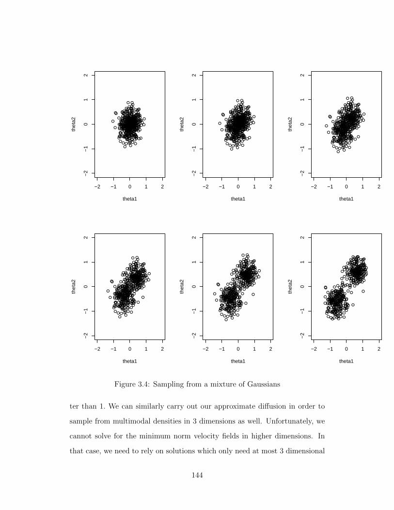
−2 −1 0 1 2

−2

−1

01

2

theta1

thet

a2

−2 −1 0 1 2−

2−

10

12

theta1

thet

a2

−2 −1 0 1 2

−2

−1

01

2

theta1

thet

a2

−2 −1 0 1 2

−2

−1

01

2

theta1

thet

a2

−2 −1 0 1 2

−2

−1

01

2

theta1

thet

a2

−2 −1 0 1 2

−2

−1

01

2

theta1

thet

a2

Figure 3.4: Sampling from a mixture of Gaussians

ter than 1. We can similarly carry out our approximate diffusion in order to

sample from multimodal densities in 3 dimensions as well. Unfortunately, we

cannot solve for the minimum norm velocity fields in higher dimensions. In

that case, we need to rely on solutions which only need at most 3 dimensional

144

integrations to do or at most 3 dimensional partial differential equations to

solve. There is one special case, where one indeed can sample by Adaptive

Annealing from a high dimensional distribution with low dimensional differen-

tial equation solvers or low dimensional integration and that is sampling from

an arbitrary multivariate Gaussian distribution as we describe in the following

section.

3.5 Sampling Multivariate Gaussians and ex-

tensions

In this section we show how to sample from an arbitrary multivariate Gaussian

distribution using Adaptive Annealing by just doing single variable integra-

tions. Inspired from the solution to the multivariate Gaussian problem, we

propose a way to solve for the velocity field in the Fokker Plank equation

in the variable augmented setting. For simplicity, let the target multivariate

Gaussian density have mean zero. The general mean situation can be han-

dled easily. Let the covariance matrix of the target be Σ1. We choose the

starting distribution to be a zero mean Gaussian with a diagonal covariance

matrix denoted by Σ0. Let us choose any smoothly varying trajectory of co-

variance matrices Σt : 0 ≤ t ≤ 1 where Σ1 is the target covariance matrix

and Σ0 is the initial covariance matrix. We denote Mt = (Σt)−1. Some ex-

amples of such a trajectory would be Σt = ((1 − t)Σ0 + tΣ1)2 or the choice

Σt = ((1− t)M0 + tM1)−1 . Then our sequence of distributions that we want

to track are N(0,Σt) : 0 ≤ t ≤ 1. Let p(t, u) denote the densities of N(0,Σt).

So we have

p(t, u) ∝ exp(−1

2uTMtu). (3.25)

145

The following Lemma says that for every t, a velocity function linear in u

satisfies the Fokker Plank pde.

Lemma 3.5.1. Let pt : 0 ≤ t ≤ 1 denote densities as in (3.25). Let Σt be

differentiable in t entrywise. Let ∂Mt

∂tbe the matrix obtained by differentiating

the matrix Mt as a function of t entrywise. Also let At be the matrix defined

as At = ∂Mt

∂tΣt. Then we have

v(t, u) = −1

2Atu (3.26)

where ∂Mt

∂tis the n × n matrix of derivatives of each entry of Mt. Then v

satisfies the Fokker Plank pde

∂ log p(u, t)

∂t= −

n∑i=1

(∂vi(t, u)

∂ui+ vi(t, u)

∂ log p(u, t)

∂ui

).

Proof. We have

log p(u, t) = −1

2uTMtu− log ct

where ct =∫Rp exp(−1

2uTMtu). Let us set v(t, u) = Atu for some matrix At

and see check whether it solves the pde we want. Let us look at the left side

of the pde. The left side of the pde turns out to be

−1

2uT∂Mt

∂tu− Ept(−

1

2uT∂Mt

∂tu).

We also have the space derivatives of log density to be

∂ log p(u, t)

∂ui= −(Mtu)i.

Hence the right side of the pde (3.5.1) becomes −∑n

i=1Ati,i + (uTAt)i(Mtu)i

which equals −Tr(At)− uTAtMtu. If the left side were to equal the right side

146

for all u then the quadratic forms have to match which implies −12∂Mt

∂t= AtMt.

Hence we have to set

At =1

2

∂Mt

∂tΣt. (3.27)

Now by theory of quadratic forms of normal random variables, we have Ept(−12uT ∂Mt

∂tu) =

Tr(Σt∂Mt

∂t). Hence we see that (3.5.1) is indeed satisfied.

The above proof shows something interesting. It tells us the right way to break

up the left side in (3.5.1) if we want to recover the solution (3.26) by just doing

one dimensional integrations. The above proof shows that the right way to try

and solve for v is to solve the following for all i = 1, . . . , n

uTAt[, i]Mt[i, ]u− At[i, i] =∂vi(t, u)

∂ui+ vi(t, u)

∂ log p(u, t)

∂ui

where At[, i] is the ith column of At and Mt[i, ] is the ith row of Mt. Solution to

the above ode’s coincide the solution (3.26). So by solving n one dimensional

ode’s which requires doing 1 dimensional integrations and estimating means

of n functions by running several chains we can recover the linear velocity

field we want (3.26). There is a price we have to pay however. We have to

estimate the means of n functions at every step and each step requires very

accurate estimation of the means otherwise the trajectories quickly become

unstable. Hence we need to make sure we have enough chains for us to be able

to estimate all the n means accurately.

This above way of sampling from a multivariate Gaussian motivates us to

explore a similar idea in the variable augmentation formulation. The goal is to

again obtain a well behaved velocity field as a solution to Fokker Plank by just

doing one dimensional integrations. In the variable augmentation formulation

147

we want to sample from the density qT as follows

qt(u) ∝ exp (T

n

n∑i=1

riφ(ui)−uTMtu

2). (3.28)

The density qt has a Gaussian term and the objective function term which is

of a product form. In light of this, we propose a path or sequence of densities

qt : 0 ≤ t ≤ 1 defined the following way

qt(u) ∝ exp (T

n

n∑i=1

riφ(ui)−uTMtu

2) (3.29)

where M0 is a diagonal matrix and M1 =I − σ2

σ2 + α2PX

α2is the target positive

definite symmetric matrix. This path qt is different that what was defined

in (3.29). There the multiplier in the exponent of the objective function term

was growing from 0 to T. This path is a lot similar to the Gaussian path

where only Mt varies smoothly with t. The difference here is that the extra

factor exp(Tn

n∑i=1

riφ(ui)) sits throughout the path. It is essential to have M0 a

diagonal matrix because then q0 is a product of one dimensional distributions

and can be efficiently sampled. For solving the equations (3.5) in the Gaussian

case we need to compute the space and time derivatives of the log densities.

The space derivatives of log qt are

∂ log q(u, t)

∂ui=T

nriφ(ui)− (Mtu)i.

This can be compared to the space derivatives of log density in the Gaussian

case.

∂ log p(u, t)

∂ui= −(Mtu)i

Since Tnriφ(ui) is very small when n >> T = O(d log d), the space derivatives

148

are almost the same as in the Gaussian case. Now we come to the time

derivative of log qt which is

∂ log q(u, t)

∂t= −1

2uT∂Mt

∂tu− Eqt(−

1

2uT∂Mt

∂tu) (3.30)

where Eqt refers to expectation with respect to the density qt.Although ∂ log q(u,t)∂t

looks exactly like ∂ log q(u,t)∂t

, it differs from the Gaussian case in the expectation

term because qt is no longer a Gaussian density. Now in the Gaussian case,

we broke up the time derivative of log pt as follows

∂ log p(u, t)

∂ui=

n∑i=1

(uTAt[, i]Mt[i, ]u− EptuTAt[, i]Mt[i, ]u

)where At is defined as in (3.27). In the Gaussian case, EptuTAt[, i]Mt[i, ]u is

known to be At[i, i]. Similarly, we can break up the time derivative of log q as

follows

∂ log q(u, t)

∂ui=

n∑i=1

(uTAt[, i]Mt[i, ]u− EqtuTAt[, i]Mt[i, ]u

)In this case EqtuTAt[, i]Mt[i, ] is unknown and hence has to be estimated from

multiple chains. So to summarize we propose solving the following bunch of

differential equations

uTAt[, i]Mt[i, ]u− EqtuTAt[, i]Mt[i, ]u =∂vi(t, u)

∂ui+ vi(t, u)

T

nriφ(ui)− (Mtu)i.

(3.31)

where at every timestep, we estimate the means of the quadratic forms EtuTAt[, i]Mt[i, ]u

from multiple chains by taking the sample average. This gives us a velocity

field which certainly satisfies the overall Fokker Plank and tries to mimic the

way we solve for a well behaved velocity field in the Gaussian case by just

149

doing one dimensional integrations. The hope is that only a small fraction

of the trajectories would be unstable and the remaining samples would be

approximately valid for our target distribution.

3.6 Conclusion

We have proposed an optimization problem motivated by high dimensional

function estimation. The problem is hard because the objective function may

be highly multimodal. We have proposed a randomized algorithm to opti-

mize such functions ala simulated annealing, only that the transition steps are

motivated by the theory of diffusions and not Markov Chain theory. The tran-

sitions are made after solving a high dimensional pde, commonly known as the

Fokker Plank equation. We have shown how to solve the pde in dimensions

one, two and atmost three. In the special case of the objective function being

the superposition of ridge functions we have also proposed a way of solving the

required pde by just doing many one dimensional integrations. The hope is to

encourage exploration solving multimodal sampling problems in high dimen-

sions and to further understand the potential of solving such hard problems

by our method of Adaptive Annealing.

3.7 Appendix

3.7.1 Proof of Lemma (3.3.1)

In the following we abuse notation by denoting any constants generically by

C. Recall f(θ) = 1n

∑ni=1 riφ(xTi θ) where φ is a smooth bounded function

150

taking values between ±1 and also has bounded derivatives. We also have the

sequence of densities defined by

pt(θ) = exp(tf(θ))exp(−1

2θTMθ)(

1√2π

)d√det(M)

where M = XTXn

as can be seen from (??). The question is how large should

t be so that Etf(θ)supθf(θ)

is no less than a constant value C. Let θ? be any point in

Rd maximizing f Since f is bounded in absolute value by 1, we note that

f(θ?) + 1

f(θ?)≥ f(θ?)− Etf(θ)

f(θ?).

We want f(θ?)−Etf(θ)f(θ?)

≤ C where C is any constant strictly less than 1, say 12. It

can be checked that ∂ log ct∂t

= Etf(θ) and ∂2 log ct∂t2

= V artf(θ) ≥ 0. So it follows

that Etf(θ) is a non decreasing function of t. An application of mean value

Theorem and the fact that log c0 = 0 now gives us

log ctt≤ Etf(θ). (3.32)

The above result gives us a way to upper bound f(θ?)− Etf(θ). Using (3.32)

we have

f(θ?)−Etf(θ) ≤ −1

tlog

∫Rd

exp(t(f(θ)−f(θ?))exp(−1

2θTMθ)(

1√2π

)d√det(M)dθ.

We can further restrict the integral on the right side of the above equation in an

ellipsoid around θ?. This cannot decrease the right side because exp(t(f(θ)−

f(θ?)) ≤ 1. Hence we have

f(θ?)−Etf(θ) ≤ −1

tlog

∫Bε

exp(t(f(θ)−f(θ?))exp(−1

2θTMθ)(

1√2π

)d√det(M)dθ

(3.33)

151

where Bε = θ : (θ−θ?)TM(θ−θ?) ≤ ε2. Now we want to say that f(θ)−f(θ?)

cannot be arbitrarily low in the set Bε. By Taylor’s expansion and the fact that

the derivative of f at θ? is 0 we have

f(θ)− f(θ?) = (θ − θ?)THf (ζ)(θ − θ?)

where ζ is some point lying between θ and θ?. The i, jth entry of the Hessian

matrix Hf is given by

∂2

∂θi∂θjf(ζ) =

1

n

n∑l=1

rlφ′′(xTl θ)XliXlj.

So the maximum eigenvalue of Hf would be atmost the maximum eigenvalue

of 1nXTX which would be atmost a constant C under most reasonable assump-

tions on the design matrix X. Then we have

∂2

∂θi∂θjf(ζ) ≤ C(θ − θ?)T (θ − θ?).

Multiplying by M and its inverse we have

∂2

∂θi∂θjf(ζ) ≤ C(θ − θ?)TM

12M−1M

12 (θ − θ?)

which further gives us

∂2

∂θi∂θjf(ζ) ≤ Cλmax(M

−1)(θ − θ?)TM(θ − θ?)

. Hence we have for all θ ∈ Bε the following

f(θ)− f(θ?) ≤ Cλmax(M−1)ε2.

152

The same argument could be repeated for −(f(θ) − f(θ?)) so that we can

obtain for all θ ∈ Bε the following

f(θ)− f(θ?) ≥ −Cλmax(M−1)ε2. (3.34)

From (3.33) and (3.34) we now have

f(θ?)−Etf(θ) ≤ Cλmax(M−1)ε2− 1

tlog

∫Bε

exp(−1

2θTMθ)(

1√2π

)d√det(M)dθ

Now it can be checked that

θTMθ ≤ 2(θ − θ?)TM(θ − θ?) + 2θ?TMθ?. (3.35)

Using the above inequality we then have

f(θ?)−Etf(θ) ≤ Cλmax(M−1)ε2−1

tlog

∫Bε

exp(ε2+θ?TMθ?)(1√2π

)d√det(M)dθ

Pulling out the exponent and the constant terms out of the integral in the

right side of the above equation we now have

f(θ?)−Etf(θ) ≤ Cλmax(M−1)ε2+

ε2 + θ?TMθ?

t+d log(2π)

2t− log detM

2t−1

tlog

∫Bε

dθ.

The log volume of the ellipsoid Bε is log detM2

plus log volume of the unit ball in

Rd as can be seen from the change of variable theorem. Also it is well known

that the log volume of the unit ball in Rd is d2

log π + d log ε − log Γ(d2

+ 1)

where Γ refers to the well known Gamma function satisfying the recurrence

property Γ(x + 1) = xΓ(x) and Γ(12) =√π. An important fact is Γ(d

2+ 1) is

153

of the order d log d. Hence combining the above facts we have the following

f(θ?)− Etf(θ) ≤ Cλmax(M−1)ε2 +

ε2 + θ?TMθ?

t+d log(2π)

2t+

1

tlog Γ(

d

2+ 1)− d

2tlog π − d

tlog ε.

Setting ε2 = d2tCλmax(M−1)+ 1

t

we have the final upper bound

f(θ?)− Etf(θ) ≤ Cλmax(M−1)

d

2tCλmax(M−1) + 1t

+

d2tCλmax(M−1)+ 1

t

+ θ?TMθ?

t+d log(2π)

2t+

1

tlog Γ(

d

2+ 1)− d

2tlog π − d

tlog ε.

From the above we see that we need t = O(d log d) so that the difference f(θ?)−

Etf(θ) is upper bounded by a constant value. Hence the ratio f(θ?)−Etf(θ)f(θ?

is

upper bounded by a constant C divided by f(θ?).

154

Bibliography

[1] A. Barron, A. Cohen, W. Dahmen, and R. DeVore, “Approximation

and learning by greedy algorithms.” Annals of Statistics, vol. 35, 2007.

[2] B. DasGupta, H. Siegelmann, and E. Sontag, “On the Intractability

of Loading Neural Networks.” Kluwer Academic Publishers, 1994, ch.

X, pp. 357389.

[3] V. Vu, “On the infeasibility of training neural networks with small

mean-squared error.”

IEEE Trans. on Information Theory, vol. 44, no. 7, pp. 28921900, 1998.

[4] N. Metropolis, A. Rosenbluth, M. Rosenbluth, A. Teller, and E. Teller,

“Equations of state calculations by fast computing machines. Journal

of Chemical Physics, vol. 21, no. 6, pp. 10871092, 1953.

[5] S. Kirkpatrick, C. D. G. Jr., and M. P. Vecchi, “Optimization by sim-

ulated annealing.” Science, vol.220, no. 4598, pp. 671-680, 1983.

[6] J. Chang, “Stochastic processes.”

http://pantheon.yale.edu/jtc5/251/stochasticprocesses.pdf.

[7] H. Risken, “The Fokker-Planck Equation: Methods of Solutions and

Applications.” Springer, 1996

155

[8] E. J. Candes, “New ties between computational harmonic analysis and

approximation theory.”

C.K. Chui, L.L. Schumaker, J. Stoeckler (Eds.), Approximation Theory

X: Wavelets, Splin, Vanderbilt Univ. Press, Nashville, TN (2002), pp.

87153

[9] M. Leshno, V. Y. Lin, A. Pinkus, S. Schocken, “Multilayer feedfor-

ward networks with a nonpolynomial activation function can approxi-

mate any function.” Neural networks 6 (6), 861-867

[10] A. R. Barron, X. Luo, “Adaptive Annealing.” 45th Annual Allerton

Conference, Allerton House, UIUC, Illinois, USA 2007.

[11] C. Villani, “Topics in Optimal Transportation.” Graduate Studies in

Mathematics 58, American Mathematical Society, Providence(2003).

156