1

Adaptive B-spline Knots Selection Using Multi-Resolution Basis Set

Yuan Yuana, Nan Chenb, Shiyu Zhouac

a Department of Industrial and Systems Engineering, the University of Wisconsin – Madison b Department of Industrial & Systems Engineering, National University of Singapore c Corresponding author. Email: szhou@engr.wisc.edu

ABSTRACT

B-splines are commonly used in the Computer Aided Design (CAD) and signal processing to fit

complicated functions because they are simple yet flexible. However, how to place the knots

appropriately in B-spline curve fitting remains a difficult problem. In this paper, we proposed a two-stage

knots placement method to place knots adapting to the curvature structures of the unknown function. At

the first stage, we selected a subset of basis functions from the pre-specified multi-resolution basis set

using the statistical variable selection method—Lasso. At the second stage, we constructed the vector

space spanned by the selected basis functions and identified a concise knots vector that is sufficient to

characterize such vector space to fit the unknown function. We demonstrated the effectiveness of the

proposed method using numerical studies on multiple representative functions.

Keywords: B-splines, Lasso, Knots selection, Free knots splines

1 INTRODUCTION

Because of their mathematical elegance and geometrical flexibility, B-splines are widely used in

engineering practice. In Computer Aided Design (CAD) and Computer Aided Engineering (CAE), B-

splines and their generalized form NURBS [3, 14, 15, 18] are used to design the product geometry, or to

reconstruct geometric models of physical parts from measurement data. In signal processing and image

processing, B-splines are often adopted to process noisy signals, or to approximate complicated functions

[19, 26].

Mathematically, a B-spline curve of pth degree is defined as the linear combination of a set of basis

functions

2

1

0, ),()(

pm

jpjj tNqtf u , (1)

where Nj,p(t,u), is the jth B-spline basis function of pth degree defined on a sequence of non-decreasing

knot values u=(u0,u1, …, um) as follows [18]

1,...,1,0),()()(

otherwise0

if1)(

1,111

11,,

10,

pmjtNuu

tutN

uu

uttN

ututN

pjjpj

pjpj

jpj

jpj

jjj

(2)

The knots vector u is often normalized to the interval [0, 1] and its boundary values are set to

u0=u1=…=up=0, um-p=um-p+1=…=um=1, referred as the open knots vector [18]. The knots vector u together

with the degree p determine the set of the B-spline basis functions, as seen from (2), Su,p = Nj,p(t),

j=0,1,…,m-p-1. The basis functions Nj,p(t), j=0,1,…,m-p-1 are linearly independent [3]. They also span

a vector space u,p consisting of the linear combinations of the basis functions

1,...,1,0 , ),( 1

0,, pmjtN

pm

jjpjjp u . (3)

The vector space u,p contains piecewise polynomial functions of degree less than or equal to p with the

elements in u as the breaking sites. Furthermore, f(t) u, p, it is jrpC

continuous at uj, and infinitely

differentiable elsewhere, where rj is the multiplicities of uj in vector u (0≤ rj ≤ p+1). The B-splines

constructed above possess many important properties, which are included in the Appendix I for easy

reference.

B-spline approximation can be constructed based on the observed data points (ti,yi), i=0,1, …, n, 0≤

ti ≤1, where ti is the independent variable and yi is the observation, by minimizing the least square

distance as follows:

n

i

pm

jipjji

qtNqy

j 0

21

0,

,),(min u

u (4)

3

where u is the knots vector and qj, j=0,1, …, m-p-1 are the control points. Clearly, to fit a B-spline

curve, both the knots vector and the control points need to be determined based on the data.

In the literature, many research works in B-spline curve fitting focused on how to optimize the control

points when the knots vector is given. Different optimal criteria and algorithms have been proposed such

as least square methods [18], weighted least square methods [1, 18], moving least square methods [10,

12], Kalman filter [7], etc. However, there are only limited works on how to choose the optimal knots

vector because of the following critical challenges. First, both the number of knots and their locations

need to be determined, which leads to an extremely large search space of the knot optimization problem.

Second, the basis functions are nonlinear in terms of knots values even if the number of knots is given,

which make the search space nonlinear. The nonlinear search space makes it difficult to find

computationally useful criteria by which an optimal approximation can be recognized and distinguished

from other approximations [3].

The existing works on knots placements can be roughly categorized into heuristic methods and

constrained optimization methods. In the class of heuristic methods, the underlying feature information of

the unknown function is utilized to select the knots number and their locations. Razdan [21] proposed a

heuristic method to firstly determine the number of knots, and then select knots in order to make the

curvature distribution and chord length distribution uniformly distributed within the knots spans.

Although this method works well for relatively smooth functions, it may result in excessive number of

knots when the function is bumpy. De Boor [3] chose knots when the knot number is fixed in such a way

that guarantees the resulting linear system in solving (4) is well-conditioned and has unique optimal

solution of control points. This method tends to distribute the knots uniformly, which will result in poor

performance if the underlying function has inhomogeneous curvatures. Li et al. [13] first smoothed the

discrete curvatures of given points and then chose the inflection points to be knots. This method has

limited choices of the knots number and locations, constrained by observed data points. In general, these

heuristic methods are sensitive to measurement noises and cannot guarantee a good approximation when

the measurement error is relatively large.

4

In the class of constrained optimization methods, the knots placement problem is formulated as a

nonlinear optimization problem and optimization techniques are applied to find the optimal knots vector.

Randrianarivony and Brunnett [20] used Levenberg-Marquardt iterative algorithm to solve the nonlinear

optimization problem. However, they need to fix the number of knots a priori and may require high

computational load if the initial guess is off. Schwetlick and Schutze [22] also fixed the knot number first

and optimize the knot locations using generalized Gauss-Newton method. In addition, they further

eliminated some knots according to certain removal criteria to find the best subsets. However, their

strategy that optimizes the knot number and locations separately might not be optimal because these two

decision variables are tightly coupled together. Moreover, the generalized Gauss-Newton method can

only find a local optimum. Recently, Miyata and Shen [16] proposed an evolutionary algorithm to jointly

optimize the knots number and locations. Their methods are computational intensive and may need fine

tuning of several parameters.

Besides the abovementioned works, there are also some methods reported to select knots for other

types of basis functions, such as truncated power basis functions [6, 17], and radial basis functions [11].

However, in those problems, one knot can only influence one basis function, which is not the case in B-

splines. Therefore, these methods cannot be applied to place the B-spline knots.

Targeting on the limitations of the existing methods, we propose a computationally efficient way to

provide effective knots placements in B-spline curve fitting. The basic idea is based on the following fact

as stated in [3]: “the approximation performance of B-spline curve fitting is not sensitive to some or all

the precise locations of knots; rather, the distribution or density of knots affects the approximation error

significantly”. In other words, instead of searching the optimal locations of individual knots, we only

need to place them approximately according to the change of function characteristics. Based on this

intuition, we propose a two-stage method to automatically find the appropriate distribution of the knots.

At the first stage, we specify a multi-resolution basis set that contains B-spline basis functions with

different curvature levels. Then we use the Lasso variable selection method to find the best basis subset

efficiently. At the second stage, we find the knots locations corresponding to the selected subset of the

5

basis functions with proper pruning. Finally, we use the resulting knots vector to construct the B-spline

basis according to (2) and fit the curve by solving (4). Our proposed method has the following merits:

first we can automatically capture the inhomogeneous curvature structures of the unknown function using

the multi-resolution basis functions; second, we reduce the computational time dramatically by selecting

the optimal basis functions instead of the knots vector directly; third, we can simultaneously find a good

combination of the knot number and knot locations, which ensures good fitting performance.

The remainder of this paper is organized as follows. In Section 2, we introduce the framework and

the details of the proposed method. In Section 3, we illustrate the effectiveness of the proposed method

through numerical studies and comparisons with existing works. Finally, in Section 4, we conclude our

paper with discussions on future research directions.

2 ADAPTIVE KNOTS PLACEMENT FOR B-SPLINE CURVE FITTING VIA LASSO

We have briefly described our method in the introduction. It consists of several critical steps, which

are illustrated in Figure 1. The critical idea of the proposed method is to create a set that contains B-spline

bases with different levels of curvatures first. Then it adaptively selects the subset of bases through Lasso

method based on the observed data. Finally it identifies the knots vector u based on the selected subset of

basis functions. As a result, our method achieves the adaptive distribution of knots. The technical details

of each step of the proposed method are presented in the following subsections.

Figure 1 Framework of proposed method.

2.1 Construct multi-resolution B-spline basis set

6

As pointed out early, a good knot placement should distribute the knots according to the changes of

the curvature of the unknown function. Mathematically, knots density or distribution can be described by

the concept of mesh size and mesh ratio [2]. Given knots vector u=(u0,u1,…,um), the mesh size of u is

defined as |τ|=maxτi, i=0,1, …, m-1, where i denotes the forward difference i =ui+1-ui. Smaller mesh

size indicates denser knots. And the mesh ratio is defined as dupmax(i+p -i) / (j+p -j), i=p+1,

p+2,…,m-p-1, |i-j|=1, where p is the degree of the B-spline . The mesh ratio measures the uniformity of

the knots distribution, and it equals 1 if the knots are uniformly distributed.

The distribution of knots also determines the resolution of the basis functions, which is reflected by

the support of the basis functions (a set in which the function value is nonzero). According to the local

support property (Property 1 in Appendix I), basis functions constructed on dense knots have narrower

support than those constructed on sparse knots. Since basis functions with narrow support are only

nonzero in a small range, they can capture larger curvature structures or finer structures. In contrast, the

basis functions with wide support influence the approximation in a large range, and can only capture

smaller curvature or coarser structures. In order to approximate functions with inhomogeneous curvature

structure, we need both high resolution basis functions and low resolution basis functions and locate

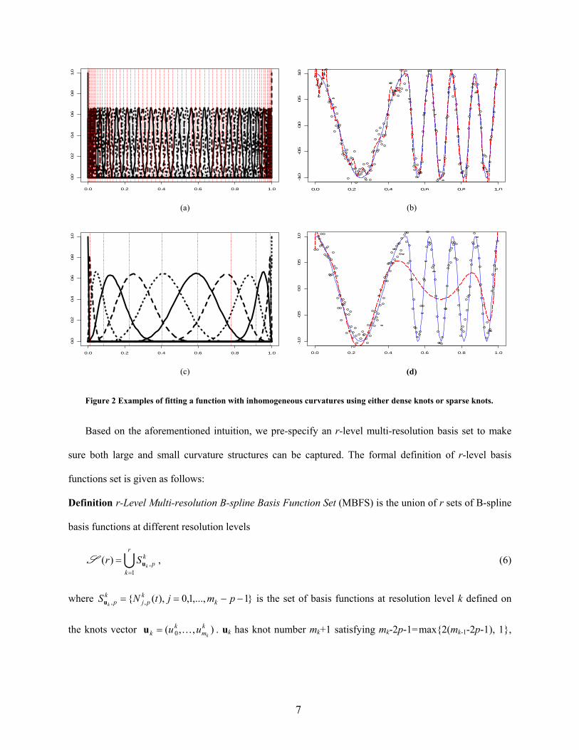
them adaptively. To demonstrate this point, Figure 2 illustrates the results of using single-resolution basis

functions to fit a function with inhomogeneous curvatures

15.0,16cos

5.00,4cos)(

tt

tttg

(5)

Figure 2 shows that neither the dense knots nor sparse knots can perform well in this case, which motivate

the needs for multi-resolution basis functions.

7

0.0 0.2 0.4 0.6 0.8 1.0

0.0

0.2

0.4

0.6

0.8

1.0

(a)

0.0 0.2 0.4 0.6 0.8 1.0

-1.0

-0.5

0.0

0.5

1.0

(b)

0.0 0.2 0.4 0.6 0.8 1.0

0.0

0.2

0.4

0.6

0.8

1.0

(c)

0.0 0.2 0.4 0.6 0.8 1.0

-1.0

-0.5

0.0

0.5

1.0

(d)

Figure 2 Examples of fitting a function with inhomogeneous curvatures using either dense knots or sparse knots.

Based on the aforementioned intuition, we pre-specify an r-level multi-resolution basis set to make

sure both large and small curvature structures can be captured. The formal definition of r-level basis

functions set is given as follows:

Definition r-Level Multi-resolution B-spline Basis Function Set (MBFS) is the union of r sets of B-spline

basis functions at different resolution levels

r

k

kpk

Sr1

,)(

uS , (6)

where 1,...,1,0),( ,, pmjtNS kk

pjk

pku is the set of basis functions at resolution level k defined on

the knots vector ),,( 0km

kk k

uu u . uk has knot number mk+1 satisfying mk-2p-1=max2(mk-1-2p-1), 1,

8

and mesh ratio satisfying 1≤ p

kdu ≤ 1.5. The boundary knots at all levels are set to 010 k

pkk uuu ,

1 1 km

kpm

kpm kkk

uuu , for k=1,2,…,r.

We would like to make some comments regarding some important properties of the MBFS. First,

though the basis functions in kpk

S ,u are linearly independent and form a basis of the vector space kpk ,u ,

the basis functions from two levels are in general linearly dependent. Second, the number of interior knots

in uk is two times of that in uk-1. Therefore, basis functions in kpk

S ,u generally have narrower support, or

higher resolution than those functions in 1,1

kpk

Su .

In the definition of MBFS, we only specify the boundary knots in uk. And we can select the internal

knots freely as long as the mesh ratio condition 1≤ p

kdu ≤ 1.5 is satisfied. In practice, we can choose the

Chebyshev points, which is proven to perform well in general [3], as the interior knots of uk. They are

defined as

)1(,),1(,22)22(2

)1)1(2(cos1

pmpj

pm

pju k

k

kj

.

(7)

Or we can simply select uniformly spaced knots, which has mesh ratio 1,

)1(,),1(,12

pmpj

pm

pju k

k

kj

.

(8)

At the first resolution level, we often set the knot number m1=2p+1, indicating that u1 has no interior

knots and is the sparsest knots vector possible. Figure 3 shows examples of the basis functions at different

resolution levels. It illustrates that basis functions in higher resolution level have higher resolution, i.e.,

smaller support. In principle, we can approximate the unknown function of arbitrary resolution level by

choosing large enough r. However, when the observations are noisy, basis functions of excessive high

resolutions tend to over fit the data and the approximation performance is very sensitive to noise. On the

other hand, basis functions of insufficient resolution might miss the finer structures of the unknown

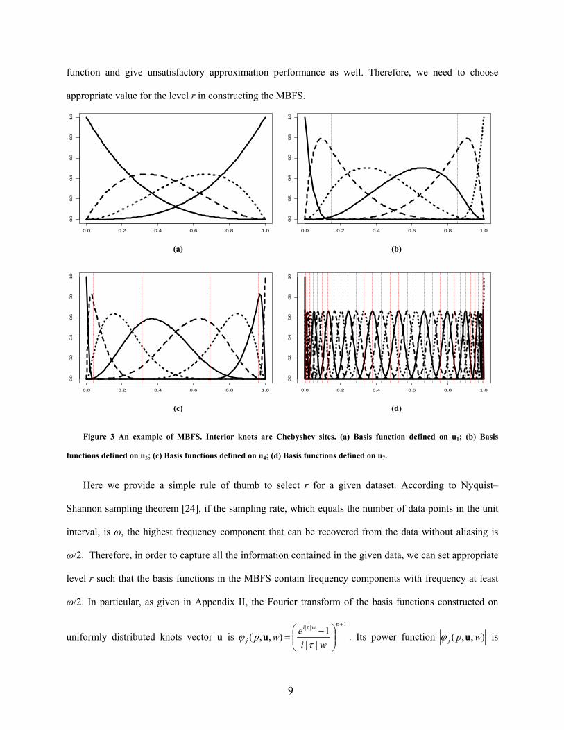
9

function and give unsatisfactory approximation performance as well. Therefore, we need to choose

appropriate value for the level r in constructing the MBFS.

0.0 0.2 0.4 0.6 0.8 1.0

0.0

0.2

0.4

0.6

0.8

1.0

(a)

0.0 0.2 0.4 0.6 0.8 1.0

0.0

0.2

0.4

0.6

0.8

1.0

(b)

0.0 0.2 0.4 0.6 0.8 1.0

0.0

0.2

0.4

0.6

0.8

1.0

(c)

0.0 0.2 0.4 0.6 0.8 1.0

0.0

0.2

0.4

0.6

0.8

1.0

(d)

Figure 3 An example of MBFS. Interior knots are Chebyshev sites. (a) Basis function defined on u1; (b) Basis

functions defined on u3; (c) Basis functions defined on u4; (d) Basis functions defined on u7.

Here we provide a simple rule of thumb to select r for a given dataset. According to Nyquist–

Shannon sampling theorem [24], if the sampling rate, which equals the number of data points in the unit

interval, is ω, the highest frequency component that can be recovered from the data without aliasing is

ω/2. Therefore, in order to capture all the information contained in the given data, we can set appropriate

level r such that the basis functions in the MBFS contain frequency components with frequency at least

ω/2. In particular, as given in Appendix II, the Fourier transform of the basis functions constructed on

uniformly distributed knots vector u is 1||

||

1),,(

pwi

j wi

ewp

u . Its power function ),,( wpj u is

10

symmetric and has multiple zeros at certain frequencies, among which its first zero is located at w=2/||

in the positive frequency range. Since the value of ),,( wpj u is almost negligible outside the interval [-

2/||, 2/||], we can approximately treat the basis function as a band limited signal with band width [-

2/||, 2/||]. If we want the basis functions in MBFS cover the frequencies of at least ω/2, the smallest

|| should at most be 4/ω, or equivalently r should at least be log2(n/4-1)+2 when m1-2p-1=0, or

112

14/log

12

pm

n when m1-2p-1 ≠ 0. The detailed derivation of this result can be found in Appendix II.

For non-uniformly distributed internal knots, e.g., Chebyshev knots, we can follow the similar idea to

identify a suitable value of r. However, we need rely on numerical methods instead of closed form

formula in such cases. We would like to point out that the above guideline only provides a lower bound

for r. If r is chosen smaller than the lower bound, the MBFS might not capture the fine features of

unknown function. In practice, r is often selected to be larger than the lower bound. And a relatively

larger r is used when the noise is small, or smaller r is used when the noise is large to avoid overfitting.

2.2 Select basis subset among S (r) via Lasso

The constructed MBFS is expected to include basis functions of different resolutions. They can

characterize both smooth features with smaller curvature and bumpy features with larger curvature.

However, it is infeasible to directly use the complete MBFS to approximate the unknown function. In

more details, MBFS often includes a large number of basis functions, often exceeding the number of

sample points. Moreover, these basis functions in MBFS are not linearly independent. Therefore, using

the complete MBFS may overfit the data and cause numerical instabilities. To overcome this difficulty,

we use the statistical variable selection method to select an appropriate subset of MBFS for function

approximation.

Given S (r), we can estimate the corresponding coefficients of each basis function by minimizing the

following objective function in the matrix form

11

1

2

2min QNQY

Q , (9)

where Trm

rmm r

qqqqqqq 122

111

211 21

Q is the vector of the unknown parameters

to be estimated, Tnyyy 21Y is the vector of observations, and

)()()()()()()(

)()()()()()()(

)()()()()()()(

,,12

,2,1

1,

1,2

1,1

2,2,122

,22,12

1,2

1,22

1,1

1,1,112

,12,11

1,1

1,21

1,1

21

21

21

nr

pmnr

pnpmnpnpmnpnp

rpm

rppmppmpp

rpm

rppmppmpp

tNtNtNtNtNtNtN

tNtNtNtNtNtNtN

tNtNtNtNtNtNtN

r

r

r

N (10)

includes the values of the basis functions evaluated at observation point t1, t2, …, tn; ||δ||2 and ||δ||1 are the

l2 and l1 norm respectively of the vector δ defined in the Euclidean space.

The first part in (9) is the conventional least square estimator, and the second part is a penalty term on

the decision variable qjk. This type of estimation is called Lasso [25] in the literature. Lasso has several

advantages compared with other variable selection and parameter estimation methods. It is numerically

more stable even when the data have small perturbation and it can shrink some coefficients to 0 exactly.

In addition, Lasso does not require that all the basis functions are linearly independent, which relax the

constraint that each knot span should contain at least one data point to avoid all-zero columns [22].

The tuning parameter λ plays an important role in (9). Intuitively, λ controls the tradeoff between the

fitting error and the smoothness of the approximation. If λ=0, the approximation tends to interpolate all

data points using the MBFS. If λ is too large, the approximation might be overly smooth and miss larger

curvatures. The optimal λ can be chosen by V-fold cross validation [27]. The V-fold cross validation,

where V =10 is commonly used, estimates the prediction errors when different λ is used. Subsequently the

optimal λ that minimizes the prediction error can be found. In more details, we first partition the data

randomly into V disjoint subsets of the equal size. Or equivalently, we partite the index set I=1,2, …, n

into V disjoint subset V

1

II , where Iα∩Iα’=Φ for all α ≠ α’. Secondly, we set aside one subset Iα, and

use the rest of the observations to estimate the parameters. We denote Y-α (Yα) and N-α (Nα) as the sub-

12

matrices of Y and N respectively, with all the rows Ii deleted (kept). Therefore, for each α, we can

estimate the parameter Q using all the samples except those in Iα, and we define

1

2

2minarg)( QQNYQ

Q . (11)

Then we can estimate the prediction error of a given λ using

V

1

2

2)()CV(

QNY . (12)

The λ that minimizes CV(λ) will be selected as the appropriate smoothing parameter in the B-spline

approximation. We can use the least angle regression procedure [5] to compute the solutions to (9) and

(12) efficiently.

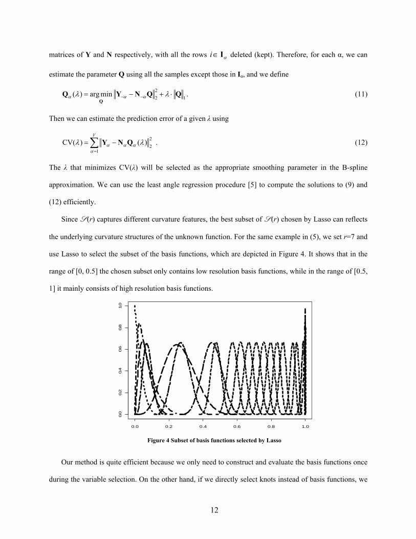
Since S (r) captures different curvature features, the best subset of S (r) chosen by Lasso can reflects

the underlying curvature structures of the unknown function. For the same example in (5), we set r=7 and

use Lasso to select the subset of the basis functions, which are depicted in Figure 4. It shows that in the

range of [0, 0.5] the chosen subset only contains low resolution basis functions, while in the range of [0.5,

1] it mainly consists of high resolution basis functions.

0.0 0.2 0.4 0.6 0.8 1.0

0.0

0.2

0.4

0.6

0.8

1.0

Figure 4 Subset of basis functions selected by Lasso

Our method is quite efficient because we only need to construct and evaluate the basis functions once

during the variable selection. On the other hand, if we directly select knots instead of basis functions, we

13

need to construct and evaluate the new basis functions every time when we drop or add a knot. This can

be very time consuming especially when the knots space is large.

2.3 Construct the knots vector from the selected subset of basis functions

The subset of basis functions selected by Lasso can often approximate the unknown function quite

well. However, because the selected basis functions are defined on different knot vectors in MBFS, the

linear combinations of them are no longer B-splines in general. Therefore, the approximation using these

basis functions does not possess some of the nice properties of B-splines. They can hardly be used in the

applications such as CAD and CAE, where only standard B-spline basis functions are accepted. In this

subsection, we propose a way to replace the selected basis functions by standard B-spline basis functions.

We denote Ω as the subset of basis functions selected by Lasso and its cardinality is mL. Let NjL(t)

denote the jth basis functions in Ω and Ω =

1,...,1,0 , , 1

0L

m

jj

Ljj mjN

L

denote the vector

space spanned by the basis functions in Ω. Lemma 1 ensures the existence of a B-spline representation of

the selected basis functions by Lasso.

Lemma 1. There exist a knots vector uL such that the vector space uL, p spanned by the B-spline basis

functions defined on uL, is a linear vector space and uL, p=Ω.

Lemma 1 can be proved using the Curry-Schoenberg Theorem. The details can be found in (e.g. [3]).

Although Lemma 1 ensures the existence of uL, it is very difficult to recover such uL given Ω. A brutal

force method is to first identify the B-spline basis functions of the vector space spanned by Ω, then to

reverse the recurrence relations in (2) to solve uL. Unfortunately, both steps are extremely difficult. To

overcome this difficulty, we propose another way around—constructing a superset of uL and then

eliminating abundant knots to find uL.

According to the local support property of the B-spline basis (Property 1 in Appendix I), each basis

function is completely determined by a small subset of the knots vector. In particular, the basis function

)(, tN kpj at the resolution level k is completely determined by the knot set ,, ,1,1,,

kppj

kpj

kpj

kpj uuu

14

regardless the other knots in the same resolution level. After finding the corresponding knots for each

basis in Ω, we can combine them together to form a new knots vector

r

k tN

kpjB

kpj1 )(

,

,

u . (13)

Here we slightly abuse the notation of the set and the operation of set union. We also would like to point

out that there might be repeated knots in uB. However, the number of repetition (or so called multiplicity)

of one knot should not be larger than p+1. We can simply delete the excessive repetitions such that the

multiplicity of any knot in uB is no more than p+1. Using this construction of uB, we have the following

theorem.

Theorem 1. Let uL denote the underlying knots vector of the vector space Ω, uB is constructed as in

(13), then uL uB.

The proof of Theorem 1 is included in the Appendix III for reference.

Although we can construct the B-spline approximation based on the knots vector uB, there are

significant redundancies which might result in excessive dimension of fitted B-splines and hence reduce

the approximation accuracy. To identify the compact knots vector uL, we need to eliminate unnecessary

knots in uB. Inspired by stepwise variable selection methods [23], we developed a stepwise pruning

algorithm to eliminate unnecessary knots in uB. We use the goodness of fit as a criterion to determine

when we should stop pruning uB.

The goodness of fit of a fitted function f(t) to a dataset (ti, yi), i = 1, 2, …, n, is often measured by

mean squared error (MSE) as

n

iii tfy

n 1

2)(1

MSE . (14)

If g(t) is the underlying true function, yi is the observation of g(ti) with additive noise εi, which has mean

zero and variance σ2, the expectation of MSE can be decomposed as:

15

n

iii

n

iii

n

iii

n

iiiii

tftgn

tftgn

tgyn

tftgtgyn

1

22

1

2

1

2

1

2

)()(1

E

)()(1

E)(1

E

)()()(1

E)MSE(E

. (15)

Clearly, even if we get a perfect fit, i.e. f(t)=g(t), E(MSE) is still σ2. Thus, if the MSE of a fitted function

f(t) is smaller than σ2, then f(t) is likely to overfit the data and the freedom of f(t) should be reduced. In

our case, this means some knots in uB should be removed. Using this criterion, the algorithm of pruning

uB can be summarized as follows.

ALGORITHM of PRUNING uB

S1: Initial knots vector ExKnots:= uB

S2: Iteration

S2.1: current knots vector CurKnots=ExKnots

S2.2: find the knot u in CurKnots such that after deleting u, the MSE has the smallest change.

S2.3: check if the MSE after deleting u is smaller than σ2. If yes, u*=CurKnots and exist.

S2.4: ExKnots = CurKnots without u. Go to S2.1.

End

The variance of the measurement error σ2 is a critical parameter in the algorithm. In practice, it might

be obtained from the specification and characteristic of the measurement equipment. In cases σ2 cannot be

accurately estimated, it can be considered as a tuning parameter in the algorithm to balance between the

model complexity and the model accuracy. To limit the scope of this paper, we do not further discuss how

to determine σ2 here. We also want to point out that this algorithm is heuristic, and may not guarantee that

the final output knots vector u* is minimally sufficient, i.e., u* = uL. Finding the minimal sufficient knots

among uB is a NP hard problem in general.

16

0.0 0.2 0.4 0.6 0.8 1.0

0.0

0.2

0.4

0.6

0.8

1.0

(a)

0.0 0.2 0.4 0.6 0.8 1.0

0.0

0.2

0.4

0.6

0.8

1.0

(b)

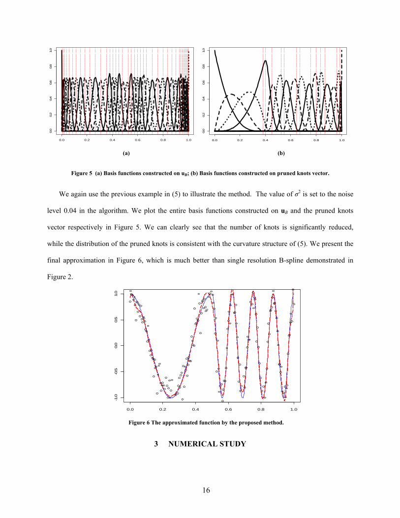
Figure 5 (a) Basis functions constructed on uB; (b) Basis functions constructed on pruned knots vector.

We again use the previous example in (5) to illustrate the method. The value of σ2 is set to the noise

level 0.04 in the algorithm. We plot the entire basis functions constructed on uB and the pruned knots

vector respectively in Figure 5. We can clearly see that the number of knots is significantly reduced,

while the distribution of the pruned knots is consistent with the curvature structure of (5). We present the

final approximation in Figure 6, which is much better than single resolution B-spline demonstrated in

Figure 2.

0.0 0.2 0.4 0.6 0.8 1.0

-1.0

-0.5

0.0

0.5

1.0

Figure 6 The approximated function by the proposed method.

3 NUMERICAL STUDY

17

In this section, we use several examples to demonstrate the effectiveness of the proposed framework.

Throughout the numerical studies, we use the cubic B-splines (p=3), and the Chebyshev sites when

constructing MBFS. We choose the tuning parameter in Lasso using 10-fold cross validation. Since we

know the true function g(t) in all the simulation studies, we use the mean squared approximation error

(MSAE), defined as ntftgn

iii /)()(

1

2

, as the performance measure of the goodness-of-fit to compare

different methods.

In Section 3.1, we use a function with inhomogeneous curvature structures to show how the adaptive

knots vector selected by the proposed method improves the approximation performance. In Section 3.2,

we compared the performance of the proposed method with some existing methods on knot selection. In

Section 3.3, we apply our method to more examples to demonstrate its effectiveness.

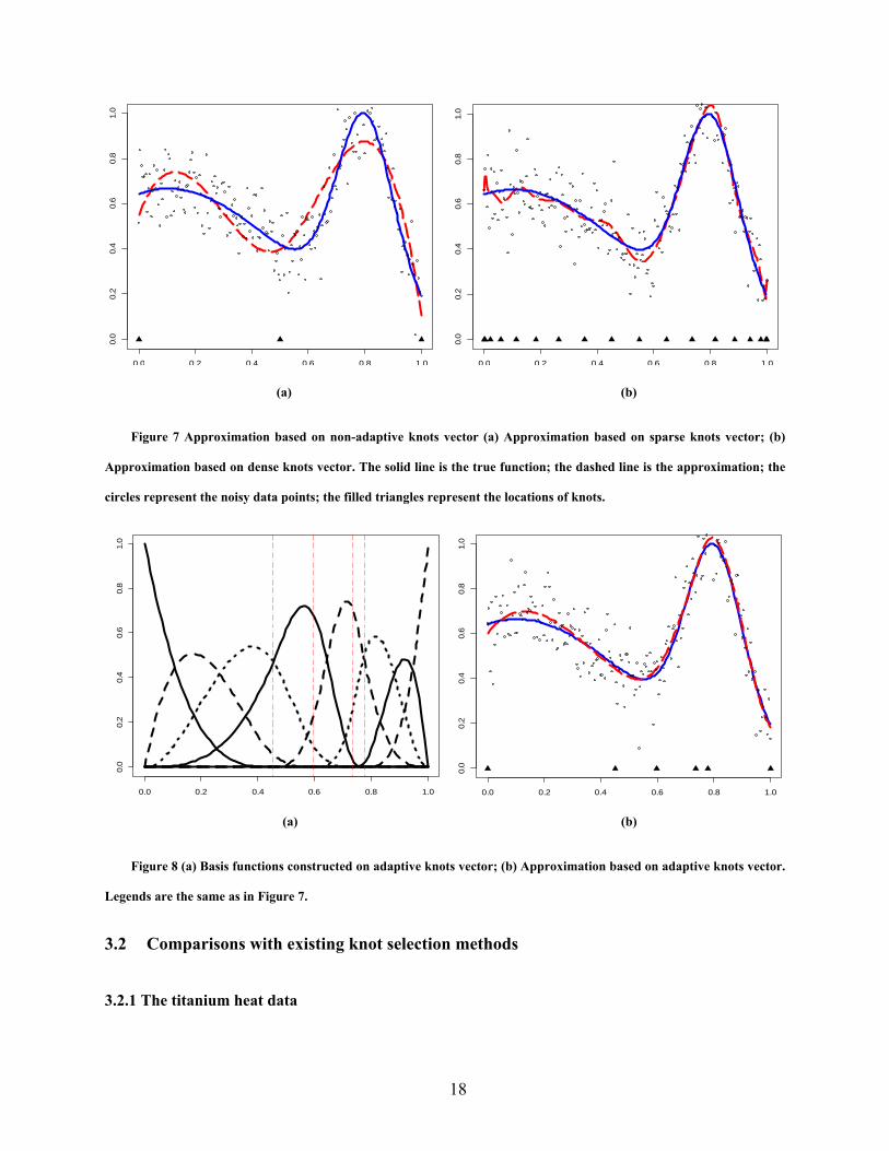
3.1 Adaptive knots vector for functions with inhomogeneous curvature structures

We uniformly sampled n=200 data points on [0, 1] from the following function

]1,0[,02.0

)8.0(exp2

2

)5.0(exp1.0

3.0

)1.0(exp5.1

3935.2

1)(

222

t

ttttg (16)

The observation error ε is normally distributed with mean 0 and standard deviation 0.1. First, we use a

sparse knots vector and a dense knots vector to fit the data, respectively. The locations of the knots are

determined using the Chebyshev method (7). Figure 7 shows the approximation performance of the B-

spline based on these two knots vectors. Not surprisingly, neither of them can approximate the function

well. We also apply the proposed method to find the adaptive locations of the knots. The parameters r and

σ2 are set to 6 and 0.01 respectively. And the basis functions constructed on the selected knots are shown

in Figure 8, together with their fitting results. It is clear that our method can place the knots adapting to

the curvature structures of the underlying functions, and as a result can approximate it well.

18

0.0 0.2 0.4 0.6 0.8 1.0

0.0

0.2

0.4

0.6

0.8

1.0

(a)

0.0 0.2 0.4 0.6 0.8 1.0

0.0

0.2

0.4

0.6

0.8

1.0

(b)

Figure 7 Approximation based on non-adaptive knots vector (a) Approximation based on sparse knots vector; (b)

Approximation based on dense knots vector. The solid line is the true function; the dashed line is the approximation; the

circles represent the noisy data points; the filled triangles represent the locations of knots.

0.0 0.2 0.4 0.6 0.8 1.0

0.0

0.2

0.4

0.6

0.8

1.0

(a)

0.0 0.2 0.4 0.6 0.8 1.0

0.0

0.2

0.4

0.6

0.8

1.0

(b)

Figure 8 (a) Basis functions constructed on adaptive knots vector; (b) Approximation based on adaptive knots vector.

Legends are the same as in Figure 7.

3.2 Comparisons with existing knot selection methods

3.2.1 The titanium heat data

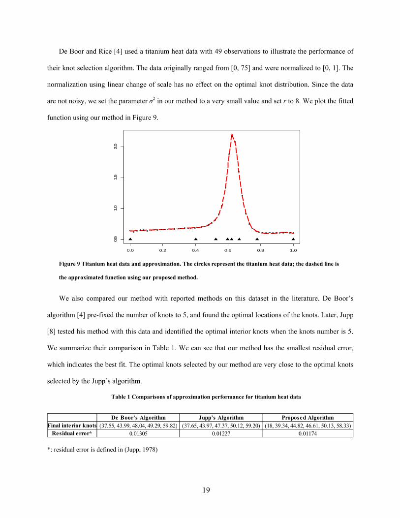
19

De Boor and Rice [4] used a titanium heat data with 49 observations to illustrate the performance of

their knot selection algorithm. The data originally ranged from [0, 75] and were normalized to [0, 1]. The

normalization using linear change of scale has no effect on the optimal knot distribution. Since the data

are not noisy, we set the parameter σ2 in our method to a very small value and set r to 8. We plot the fitted

function using our method in Figure 9.

0.0 0.2 0.4 0.6 0.8 1.0

0.5

1.0

1.5

2.0

Figure 9 Titanium heat data and approximation. The circles represent the titanium heat data; the dashed line is

the approximated function using our proposed method.

We also compared our method with reported methods on this dataset in the literature. De Boor’s

algorithm [4] pre-fixed the number of knots to 5, and found the optimal locations of the knots. Later, Jupp

[8] tested his method with this data and identified the optimal interior knots when the knots number is 5.

We summarize their comparison in Table 1. We can see that our method has the smallest residual error,

which indicates the best fit. The optimal knots selected by our method are very close to the optimal knots

selected by the Jupp’s algorithm.

Table 1 Comparisons of approximation performance for titanium heat data

De Boor’s Algorithm Jupp’s Algorithm Proposed AlgorithmFinal interior knots (37.55, 43.99, 48.04, 49.29, 59.82) (37.65, 43.97, 47.37, 50.12, 59.20) (18, 39.34, 44.82, 46.61, 50.13, 58.33)

Residual error* 0.01305 0.01227 0.01174

*: residual error is defined in (Jupp, 1978)

20

We would like to comment further on the comparison result. Although our method selected 6 knots

rather than 5, the comparison is still fair. In our method, we do not specify the knot number in advance,

and the 6 knots are automatically selected by the algorithm. In contrast, both De Boor’s and Jupp’s

methods are not able to find the appropriate number of knots, which is a critical problem in the knot

selection problem.

3.2.2 Schwetlick’s method

Schwetlick and Schutze [22] formulated the knot placement problem as a nonlinear optimization

problem and used generalized Gauss-Newton method to get the optimal solution. In their paper, they

sampled 90 equidistant points from function )1001/(10)( 2tttg in [-2, 2] and the random noise was

chosen as pseudo random numbers with -0.05 ≤ I ≤ 0.05. For easy calculation, we also normalized the

values of function g in [-2, 2] to [0, 1]. We set the parameter r=9 and the σ2 using the fitting result of

Lasso, which is 0.0007501. The fitting results and the final knots selected by the proposed method are

shown in Figure 10.

As seen from Figure 10, we selected total 6 interior knots and the MSE of the approximation is

0.0674718 compared with 0.0739568, which is calculated based on ||y-B||22 in Schwetlick’s algorithm

with 5 interior knots. However the MSAE of our fit is only 0.01519576, which indicates that our method

does not overfit the data. Therefore, our method performed better than the algorithm in [22]. Figure 10

also demonstrates that our method can adaptively select knots according to the underlying curvature

structures of the unknown function. The selected knots are quite dense when the function changes rapidly

around 0.5, while the knots are sparse in the area with small curvatures.

3.2.3 Comparisons with the Adaptive Free-Knots Splines (AFKS)

We also compared our method with another free knots spline, the AFKS, which also simultaneously

determine the knots number and locations optimally. We used the same two benchmark functions in [16]

to compare the proposed method with AFKS method. The first one is a discontinuous function defined as

follows:

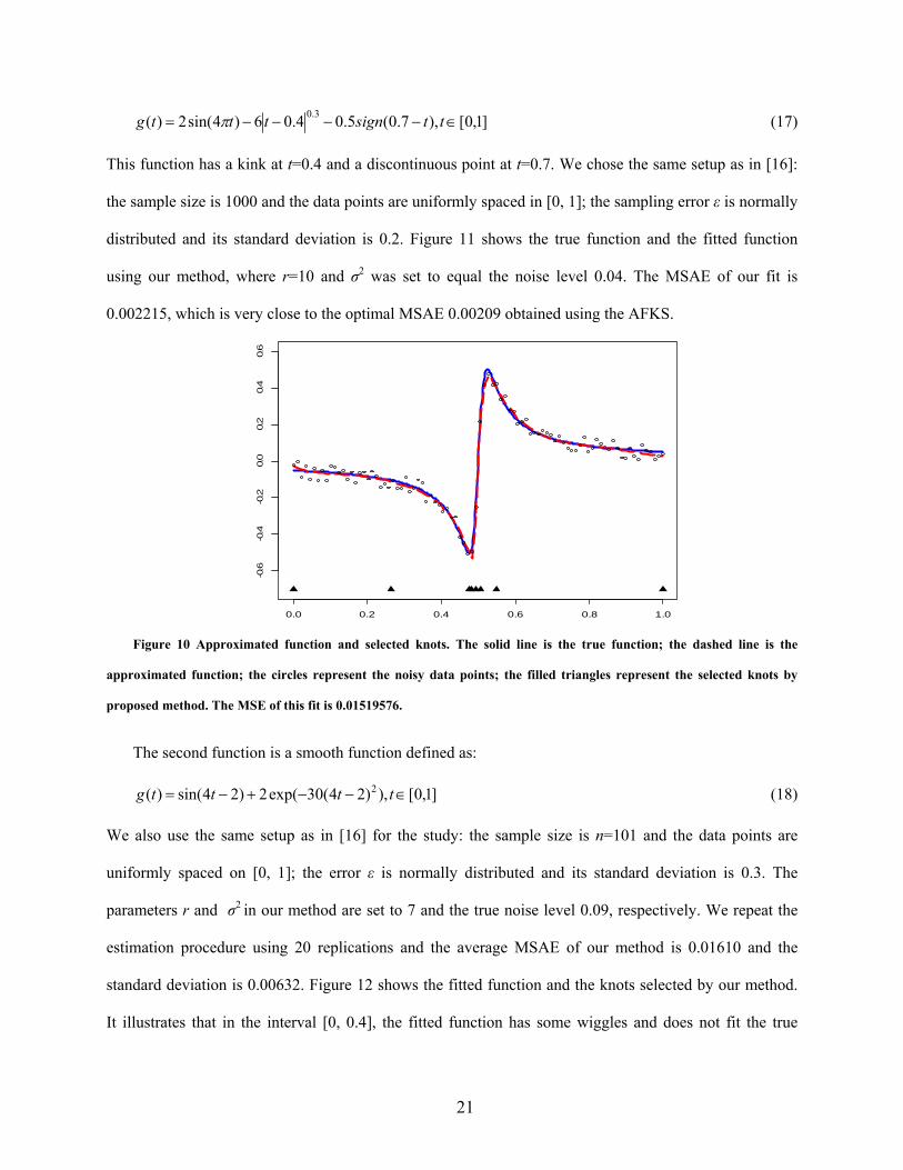
21

]1,0[),7.0(5.04.06)4sin(2)(3.0 ttsigntttg (17)

This function has a kink at t=0.4 and a discontinuous point at t=0.7. We chose the same setup as in [16]:

the sample size is 1000 and the data points are uniformly spaced in [0, 1]; the sampling error ε is normally

distributed and its standard deviation is 0.2. Figure 11 shows the true function and the fitted function

using our method, where r=10 and σ2 was set to equal the noise level 0.04. The MSAE of our fit is

0.002215, which is very close to the optimal MSAE 0.00209 obtained using the AFKS.

0.0 0.2 0.4 0.6 0.8 1.0

-0.6

-0.4

-0.2

0.0

0.2

0.4

0.6

Figure 10 Approximated function and selected knots. The solid line is the true function; the dashed line is the

approximated function; the circles represent the noisy data points; the filled triangles represent the selected knots by

proposed method. The MSE of this fit is 0.01519576.

The second function is a smooth function defined as:

]1,0[),)24(30exp(2)24sin()( 2 ttttg (18)

We also use the same setup as in [16] for the study: the sample size is n=101 and the data points are

uniformly spaced on [0, 1]; the error ε is normally distributed and its standard deviation is 0.3. The

parameters r and σ2 in our method are set to 7 and the true noise level 0.09, respectively. We repeat the

estimation procedure using 20 replications and the average MSAE of our method is 0.01610 and the

standard deviation is 0.00632. Figure 12 shows the fitted function and the knots selected by our method.

It illustrates that in the interval [0, 0.4], the fitted function has some wiggles and does not fit the true

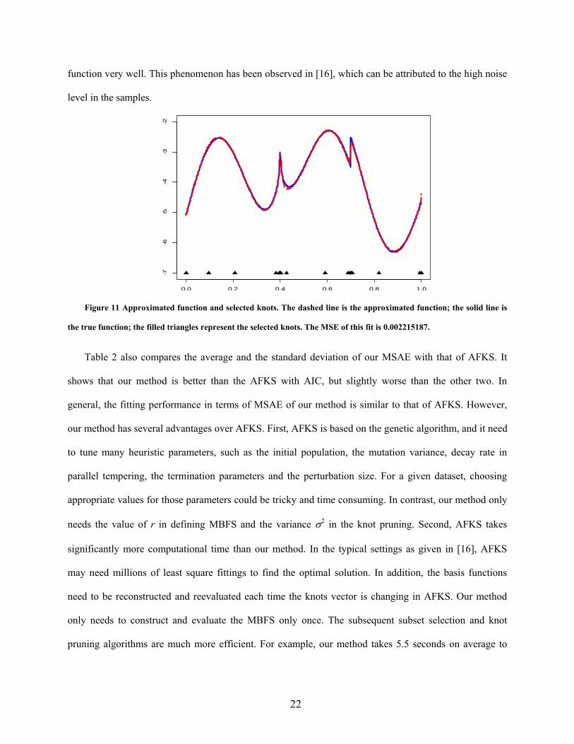
22

function very well. This phenomenon has been observed in [16], which can be attributed to the high noise

level in the samples.

0.0 0.2 0.4 0.6 0.8 1.0

-7-6

-5-4

-3-2

Figure 11 Approximated function and selected knots. The dashed line is the approximated function; the solid line is

the true function; the filled triangles represent the selected knots. The MSE of this fit is 0.002215187.

Table 2 also compares the average and the standard deviation of our MSAE with that of AFKS. It

shows that our method is better than the AFKS with AIC, but slightly worse than the other two. In

general, the fitting performance in terms of MSAE of our method is similar to that of AFKS. However,

our method has several advantages over AFKS. First, AFKS is based on the genetic algorithm, and it need

to tune many heuristic parameters, such as the initial population, the mutation variance, decay rate in

parallel tempering, the termination parameters and the perturbation size. For a given dataset, choosing

appropriate values for those parameters could be tricky and time consuming. In contrast, our method only

needs the value of r in defining MBFS and the variance 2 in the knot pruning. Second, AFKS takes

significantly more computational time than our method. In the typical settings as given in [16], AFKS

may need millions of least square fittings to find the optimal solution. In addition, the basis functions

need to be reconstructed and reevaluated each time the knots vector is changing in AFKS. Our method

only needs to construct and evaluate the MBFS only once. The subsequent subset selection and knot

pruning algorithms are much more efficient. For example, our method takes 5.5 seconds on average to

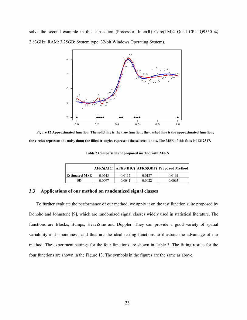
23

solve the second example in this subsection (Processor: Inter(R) Core(TM)2 Quad CPU Q9550 @

2.83GHz; RAM: 3.25GB; System type: 32-bit Windows Operating System).

0.0 0.2 0.4 0.6 0.8 1.0

-2-1

01

2

Figure 12 Approximated function. The solid line is the true function; the dashed line is the approximated function;

the circles represent the noisy data; the filled triangles represent the selected knots. The MSE of this fit is 0.01212317.

Table 2 Comparisons of proposed method with AFKS

AFKS(AIC) AFKS(BIC) AFKS(GDF) Proposed Method

Estimated MSE 0.0245 0.0112 0.0127 0.0161SD 0.0097 0.0041 0.0022 0.0063

3.3 Applications of our method on randomized signal classes

To further evaluate the performance of our method, we apply it on the test function suite proposed by

Donoho and Johnstone [9], which are randomized signal classes widely used in statistical literature. The

functions are Blocks, Bumps, HeaviSine and Doppler. They can provide a good variety of spatial

variability and smoothness, and thus are the ideal testing functions to illustrate the advantage of our

method. The experiment settings for the four functions are shown in Table 3. The fitting results for the

four functions are shown in the Figure 13. The symbols in the figures are the same as above.

24

0.0 0.2 0.4 0.6 0.8 1.0

-20

24

68

0.0 0.2 0.4 0.6 0.8 1.0

01

23

45

6

0.0 0.2 0.4 0.6 0.8 1.0

-6-4

-20

24

0.0 0.2 0.4 0.6 0.8 1.0

-10

-50

51

0

Figure 13 Randomized signal classes. Top left: Block; Top right: Bump; Bottom left: HeaviSine; Bottom right:

Doppler.

Table 3 Experimental settings for randomized signal class

Sample Size Standard Deviation of Noise

Block 101 0.5Bump 201 0.3

HeaviSine 201 0.3Doppler 112 0.1

We also apply Jupp’s method [8] on the same set of data for each function with the same number of

knots and the MSAE comparisons with our method are summarized in Table 4. As we can see our method

generally has more than 30% of improvement.

25

Table 4 Comparison with Jupp’s method

Proposed Method Jupp's Method

Block 0.3110 0.5937Bump 0.1503 0.2013

HeaviSine 0.0260 0.0440Doppler 3.7376 5.5623

4 CONCLUSION

In this paper, we proposed a new knots placement method for B-spline curve fitting. Our method

significantly reduces the searching space of the feasible knots values, while still keeping the flexibility to

distribute the knots adaptively according to the curvature structure of the underlying functions. We first

construct a multi-resolution basis set, which contains basis functions at different resolutions. Then we use

Lasso to find a concise subset of the basis functions that can fit the data well. Finally we find the knots

vector using a stepwise pruning method. Our method is demonstrated to be effective through multiple

numerical examples.

Nevertheless, there are also some open questions that we have not explored in this study. First, we

have provided some heuristic guidelines to choose appropriate values of the two tuning parameters r and

2 in the paper. However, we may investigate theoretically how to identify the optimal values of the

tuning parameters, and what are their effects on the approximation performance. Second, our knot

pruning algorithm cannot guarantee that the obtained knots vector is optimal, i.e., minimally sufficient. It

will be interesting to find a way to check whether the pruning is optimal, and quantify the gap between

current knots and the optimal knots in appropriate measures. Third, it is worthwhile to extend the

proposed method to B-spline surfaces and generalized NURBS curves or surfaces. B-spline surfaces are

defined as the tensor product of two one-dimensional B-spline curves. We can simply extend our method

by applying it to each dimension separately in B-spline surface fitting. However, we may improve the

performance by considering the joint optimization of two dimensions. In the future, we will continue

investigating the aforementioned issues along this research direction.

26

APPENDICES

Appendix I: Properties of B-spline basis functions and B-spline curves

1. Local support property. 0)(, tN pj if t is outside the interval ),[ 1 pjj uu . For any given knot

span ),[ 1jj uu , at most p+1 of pjN , are nonzero, namely pjppj NN ,, ,, . This property ensures the

change of one knot value doesn’t influence the whole curve.

2. Partition of unity. Given a knot span ),[ 1jj uu , j

pjk pk tN 1)(1, for all ),[ 1 jj uut .

3. Linearly Independent. All pth degree B-spline basis functions defined on knots vector u are linearly

independent and form the basis for vector space, u,p . Given knots number m+1, the dimension of

u,p is m-p.

4. Derivative. All derivatives of )(, tN pj exist in the interior of a knot span. At a knot uj, )(, tN pj is (p- rj)

times continuously differentiable, where rj is the multiplicities of the knot, 0≤ rj ≤ p+1. If a function

fu,p, then f is at least (p- rj) times continuously differentiable at uj and is infinitely continuously

differentiable interior of a knot span. f0u,p such that f0 is exactly (p- rj) times continuously

differentiable at uj.

5. Knot insertion property. If uu , the basis functions 1,,1,0, , pmjN pj defined on u can

be expressed as a linear combinations of 1,,1,0, , pmjN pj defined on u. Consequently, the

vector space p,u is a subspace of the vector space u,p.

6. Affine transformation invariance. If a function can be expressed as linear combinations of basis of

vector space u,p, then the affine transformation is applied to the function by applying it to the control

points, i.e. the coefficients of basis functions.

Appendix II: Fourier transforms of B-spline basis functions

27

Given knots vector u=(u0,u1,…,um), the Fourier transform of Nj,p ,the jth B-spline basis function of

pth degree defined on u, is:

jp

jkk

iwup

iwtpjj ue

iw

pdtetNwp k

1

1, )(/)(

)!1()(),,( u (19)

where

jp

jkkutt

1

)()( , represents frequency and .

For uniformly distributed knots, the Fourier transform of basis functions can be simplified as:

1||

||

1),,(

pwi

j wi

ewp

u (20)

where || is the mesh size of u.

For basis functions defined on uniform knots, we can set appropriate value for r of MBFS according

to the above results. If || is at most 4/n, then the number of interior knots of the knots vector for level r

should be at least 1/||-1=n/4-1. Since in MBFS we set the number of interior knots in such a way that

mk-2p-1=max (2(mk-1-2p-1),1), then

m1-2p-1=0 m2-2p-1=1, mr-2p-1=2r-2 r log2(n/4-1)+2

mr-2p-1 (n/4-1)

Otherwise if m1-2p-1≠ 0

m1-2p-1≠ 0 mr-2p-1=2r-1(m1-2p-1) r 112

14/log

12

pm

n .

mr-2p-1 (n/4-1)

Appendix III: Proof of Theorem 1

To prove theorem 1, we first introduce the following lemma and then use this lemma to finish the

proof.

Lemma 2. For two knots vectors u1 and u2, u2,p u1,p

if and only if u2 u1.

28

Proof : It is obvious that u2 u1 pp ,, 12 uu by the knot insertion property of B-spline basis

functions. Therefore, we only need to prove pp ,, 12 uu u2 u1. We can use the reduction-to-

absurdity method to prove this argument.

Case 1: pp ,, 12 uu but u u2 and u u1.

u u1 u is an interior point. According to the Property 4 in Appendix I, f(t) p,1u , f(t) is

infinitely differentiable at u. On the other hand, u u2 and h(t) p,2u such that h(t) is only p-k time

differentiable at u, where k is multiplicities of u in u2. Therefore h(t) p,2u , but h(t) p,1u , which

contradicts to pp ,, 12 uu . We conclude that such u doesn’t exist.

Case 2: pp ,, 12 uu . u u2 and u u1, but the multiplicities of u in u2 is m, the multiplicities

of u in u1 is n, m>n.

Again, according to the Property 4 in Appendix I, f(t) p,1u , f(t) is at least p-n times

differentiable at u and h(t) p,2u , h(t) is at least p-m times differentiable at u. We also know h0(t)

p,2u which is exactly p-m times differentiable at u. Since m>n, p-m<p-n and h0(t) p,1u . This

contradicts to pp ,, 12 uu . We conclude that m<n.

In all, pp ,, 12 uu u2 u1.

Proof of Theorem 1:

We first prove that ΩuB,p. According to the local support property of B-spline basis (Property 1 in

Appendix I), for each NjL(t) in Ω, we could find its defining knots. Without loss of generality, we assume

the defining knots for NjL(t) is ,, ,1,1,,

kppi

kpi

kpi

kpi uuu for some k1, 2, …, r and some i0, 1,

…, mk-2p-2. From the definition of uB, we know kpi, uB and thus Nj

L(t) uB,p according to the knot

29

insertion property (Property 5 in Appendix I). Because all the bases of Ω belong to uB,p, we have

ΩuB,p.

Then we use the results in Lemma 2, ΩuB,p uL uB.

5 ACKNOLEDGEMENT

The authors gratefully appreciate the editor and the referees for their valuable comments and

suggestions. This research is supported by ? and Singapore AcRF Tier 1 Funding R-266-000-057-133.

6 REFERENCE

[1] Alexa, M., Behr, J., Cohen-Or, D., Fleishman, S., Levin, D. and Silva, C. T. (2003). Computing and Rendering Point Set Surfaces. IEEE Transactions on visualization and computer graphics, 9(1): 3-15.

[2] De Boor, C. (1976). A Bound on the $L_\Infty$-Norm of $L_2$-Approximation by Splines in Terms of a Global Mesh Ratio. Mathematics of computation, 30(136): 765-771.

[3] De Boor, C. (2001). A Practical Guide to Splines, Springer Verlag. [4] De Boor, C. and Rice, J. R. (1968). Least Squares Cubic Spline Approximation, Ii-

Variable Knots, Computer Science Technical Reports, Purdue University. [5] Efron, B., Hastie, T., Johnstone, I. and Tibshirani, R. (2004). Least Angle Regression.

The Annals of Statistics, 32(2): 407-499. [6] He, X., Shen, L. and Shen, Z. (2001). A Data-Adaptive Knot Selection Scheme for

Fitting Splines. IEEE Signal Processing Letters, 8(5): 137-139. [7] Huang, Y., Qian, X. and Chen, S. (2009). Multi-Sensor Calibration through Iterative

Registration and Fusion. Computer-Aided Design, 41(4): 240-255. [8] Jupp, D. L. B. (1978). Approximation to Data by Splines with Free Knots. SIAM Journal

on Numerical Analysis: 328-343. [9] Kremer, M., Minner, S. and Van Wassenhove, L. N. (2010). Do Random Errors Explain

Newsvendor Behavior? Manufacturing & Service Operations Management, 12(4): 673-681.

[10] Lancaster, P. and Salkauskas, K. (1981). Surfaces Generated by Moving Least Squares Methods. Mathematics of Computation, 37(155): 141-158.

[11] Leitenstorfer, F. and Tutz, G. (2007). Knot Selection by Boosting Techniques. Computational Statistics & Data Analysis, 51(9): 4605-4621.

[12] Levin, D. (1998). The Approximation Power of Moving Least-Squares. Mathematics of Computation, 67(224): 1517-1532.

[13] Li, W., Xu, S., Zhao, G. and Goh, L. P. (2005). Adaptive Knot Placement in B-Spline Curve Approximation. Computer-Aided Design, 37(8): 791-797.

[14] Ma, W. and Kruth, J. P. (1995). Parameterization of Randomly Measured Points for Least Squares Fitting of B-Spline Curves and Surfaces. Computer-Aided Design, 27(9): 663-675.

30

[15] Ma, W. and Kruth, J. P. (1998). Nurbs Curve and Surface Fitting for Reverse Engineering. The International Journal of Advanced Manufacturing Technology, 14(12): 918-927.

[16] Miyata, S. and Shen, X. (2003). Adaptive Free-Knot Splines. Journal of Computational and Graphical Statistics, 12(1): 197-213.

[17] Osborne, M., Presnell, B. and Turlach, B. (1998). Knot Selection for Regression Splines Via the Lasso. Computing Science and Statistics, 30: 44-49.

[18] Piegl, L. A. and Tiller, W. (1997). The Nurbs Book, Heidelberg, Germany, Springer Verlag.

[19] Precioso, F., Barlaud, M., Blu, T. and Unser, M. (2003). "Smoothing B-Spline Active Contour for Fast and Robust Image and Video Segmentation." International Conference on Image Processing, 137-140, Barcelona, Spain, IEEE.

[20] Randrianarivony, M. and Brunnett, G. (2002). "Approximation by Nurbs Curves with Free Knots." Proceedings of the Vision, Modeling, and Visualization Conference, 195-201, Erlangen, Germany.

[21] Razdan, A. (1999). Knot Placement for B-Spline Curve Approximation, Technical Report, Arizona State University.

[22] Schwetlick, H. and Schütze, T. (1995). Least Squares Approximation by Splines with Free Knots. BIT Numerical Mathematics, 35(3): 361-384.

[23] Seber, G. A. F. and Lee, A. J. (2003). Linear Regression Analysis, Hoboken, NJ, John Wiley & Sons.

[24] Shannon, C. E. (1949). Communication in the Presence of Noise. Proceedings of the IRE, 37(1): 10-21.

[25] Tibshirani, R. (1996). Regression Shrinkage and Selection Via the Lasso. Journal of the Royal Statistical Society. Series B (Methodological), 58(1): 267-288.

[26] Unser, M., Aldroubi, A. and Eden, M. (1993). B-Spline Signal Processing. Ii. Efficiency Design and Applications. IEEE Transactions on Signal Processing, 41(2): 834-848.

[27] Wahba, G. (1990). Spline Models for Observational Data, Philadelphia, PA, Society for Industrial Mathematics.