Embed Size (px)
Citation preview

ADAPTIVE COMPENSATION BASED ACTUATOR FAULT TOLERANT
CONTROL OF NONLINEAR UNCERTAIN SYSTEMS WITH EMPHASIS ON
TRANSIENT PERFORMANCE IMPROVEMENT
A
thesis submitted
for the award of the degree of
DOCTOR OF PHILOSOPHY
by
ARGHYA CHAKRAVARTY
Department of Electronics and Electrical Engineering
Indian Institute of Technology Guwahati
Guwahati - 781 039, INDIA.
NOVEMBER 2018
TH-2198_11610211

ADAPTIVE COMPENSATION BASED ACTUATOR FAULT TOLERANT
CONTROL OF NONLINEAR UNCERTAIN SYSTEMS WITH EMPHASIS ON
TRANSIENT PERFORMANCE IMPROVEMENT
ARGHYA CHAKRAVARTY
TH-2198_11610211

Certificate
This is to certify that the thesis entitled “ADAPTIVE COMPENSATION BASED AC-
TUATOR FAULT TOLERANT CONTROL OF NONLINEAR UNCERTAIN SYSTEMS
WITH EMPHASIS ON TRANSIENT PERFORMANCE IMPROVEMENT", submitted
by Arghya Chakravarty (11610211), affiliated to the Department of Electronics and Electrical En-
gineering, Indian Institute of Technology Guwahati, for the award of the degree of Doctor of Philos-
ophy, is a record of an original research work carried out by him under my supervision and guidance.
The thesis has fulfilled all requirements as per the regulations of the Institute and in my opinion
has reached the standard needed for submission. The results embodied in this thesis have not been
submitted to any other University or Institute for the award of any degree or diploma.
Dated: Dr. Chitralekha Mahanta
Guwahati. Professor
Dept. of Electronics and Electrical Engg.
Indian Institute of Technology Guwahati
Guwahati - 781039, India.
TH-2198_11610211

To my beloved mother Mrs. Banani Chakravarty, the memory of my
father Mr. Ashoke Chakravarty and
my research inspiration Professor Francesco Bullo
I have an angel watching over me an I call him my Father. I would always remember the things
you taught me and how much you did love me. I have no words to acknowledge the sacrifices
you and mother made and the dreams you both had to let go, just to give me the opportunity to
achieve mine.
“To leave everything to the fate and to not actively contribute to the music of the universe is a sign
of sheer ignorance. You might not change your instrument, but how well you play is entirely upto
you. Whatever happens in your life, no matter how troubling things might seem, do not enter the
neighbourhood of despair. Even when all doors remain closed, God will open up a new path only
for you. Be thankful! for not only what you have been given but also for what you have been
denied...!”
-from The Forty Rules of Love by Elif Shafak
TH-2198_11610211
Acknowledgement
First and foremost, I am grateful to Almighty for having guided me through the righteous path
and bestowed upon me his grace to complete this PhD thesis successfully.
I take this opportunity to express my deepest gratitude and heartfelt thanks to my thesis advisor
Prof. Chitralekha Mahanta for her incisive expertise, consistent guidance and her intense support. I am
extremely grateful to her for giving me the opportunity to pursue a research career and introducing me
to the field of robust adaptive control theory. Her unmatched supervision, support and untiring efforts
(given that I was a direct entrant into Ph.D. after my B. Tech.) ever since the days I joined the Institute
eventually made me a successful researcher I am today. Her sincere dedication, accessibility and keen
attention to minor details in my research were of immense motivation to me. I must acknowledge her
kindness, patience and extreme diligence in correcting all my manuscripts.
I would always be indebted to my doctoral committee chair Dr. Indrani Kar for her constructive
criticisms of my work, her generous support in all possible ways she could and her trust on me more
than what I deserve. Some of her bright thoughts were very helpful in shaping up my thoughts and
were beneficial to my research. My deep appreciation and sincere thanks to her. Words would not
be enough to express my sincere gratitude towards her for the guidance, constant encouragement and
support she has imparted me throughout my PhD tenure in IIT Guwahati. I would really miss my
daily discussions with her and most specifically, the delicious chocolate truffle cakes she gifted me every
year on my birthday on New Year mornings.
I owe a debt of gratitude to other members of my doctoral committee, Dr. Srinivasan Krishnaswamy
and Dr. Sisir Kumar Nayak for devoting their precious time in evaluating the progress of my research.
Their critique and quality inputs counseled on timely basis have been of great help to me. I am thankful
to the Ministry of Human Resource Development (MHRD), Government of India for providing me the
necessary fellowship grant to pursue the Ph.D programme.
A special thanks and admiration to the person, I share a strong bond of friendship with, my dear
friend Tousif Khan Nizami. Thank you for having stood beside me against all odds and being there
for me in both difficult and good times during my stay. Your consistent encouragement and faith in
my abilities have helped me immensely to overcome the challenges and finally led to the successful
completion of this thesis. I am extremely thankful to Dr. Sanjoy Mondal (now at NTU Singapore) for
his guidance and I should submit that a greater share of the knowledge and ability I have gathered so
far in research, should be accredited to him. I also extend my deep sense of gratitude to my dearest
friends Rohan Kumar Das (now at NUS, Singapore), Saurabh Pandey (now at Dalian University of
Technology, China), Abdul Basit Andrabi, Tasaduq Hussain and Karteek for their constant motivating
discussions, support and joyful company. Especially, I am greatly indebted in Saurabh and Basit for
vTH-2198_11610211

supporting and upholding my confidence and sanguineness in all possible ways throughout the days of
writing this research monograph. I deeply appreciate their efforts in keeping me happy and bearing
with me all throughout my final struggling days at IIT Guwahati. During my toughest times here in
Guwahati, Basit’s intense support and guidance being my dearest brother, have been invaluable and
certainly beyond words. Though I have been miles apart from my family, I should definitely admit
that my years at IIT Guwahati had been like staying at home away from home in the company of these
wonderful people. I greatly acknowledge the help from my colleague and friend Manmohan Sharma in
the experimental realization of the algorithms in this thesis.
I would also like to acknowledge the love and encouragement from my dear friends Murat (Anirud-
dha Mazumdar), Abhijit Mazumdar and Nayanjyoti Kakoti. Just expressing gratitude to the un-
conditional and unparalleled support from my international friends Babba Ali Jraisheh, Grandfather
Moustafa Najm, Anne Ghadir Nofal, çocuk Ahmad AlMamo, Sami AlIssa and Malek AlHasan, would
not be enough and I would always be indebted in them for their kindness and deep affection for me.
I would also like to take this opportunity to thank Mr. Nizam Ali Khan (Tousif’s father) for bestow-
ing his affection on me and our thought-provoking discussions which have helped me immensely all
throughout my journey so far.
This journey would not have been complete without the love and affection of my dear friends Vinay
Kumar Pandey (now R&D Scientist in Mercedes, Germany), Pravin Kumar Chaturvedi, Vibhuti Ku-
mar, Khalid Wani, Syed Zainul Aabidin, Ankit Bansal, Resmi N. Chandrasekharan (Chechi), Subhasis
Mandal, Nabanita Adhikary, Jyoti Prakash Medhi & his family, Jasvindar Singh, Shadab Illahi, Ajaz
Ahmad Dar, Deepak Joshi and Satyabrata Dash. Also, my acknowledgment to my faculty and friend
Mrs. Papiya Debnath for her confidence in my worthiness.
I am grateful to the staff of the Academic Section at IIT Guwahati, Mr. Manas Sarma in particular,
and Mr. Sidananda Sonowal, for their valuable advice, encouragement and kind assistance in all times
throughout my PhD tenure. I also extend my thankfulness to Mrs. Kajallata Brahma and Mrs.
Trishna Choudhury for their generous help and cooperation in regards to the formalities involved in
potential funding for my research visit to France in July 2017. I soulfully thank my colleagues from
Control & Instrumentation Laboratory, who have made this journey, a learning and a joyful experience.
Among them my appreciation to Dr. Bajarangbali, Dr. Ezhil Reena Joy, Mandar Maitra, Madhulika
Das, Mridul K. Malakar, Gautam Rituraj, Kamakshi Manjari, Suman Roy, Mriganka Biswas and
Karnika Biswas. Last but definitely not the least, I do not find words to describe the extent of debt
I owe to my family. The unlimited sacrifices and relentless hardwork of my mother Mrs. Banani
Chakravarty and my sister Ananya Chakravarty have been truly motivating and been a consistent
source of encouragement to me. The contributions of my Godfather Mr. Satyabrata Jana, Mrs.
Subhra Jana and Mrs. Dolly Bose (Madame) are much beyond words and I feel privileged to have had
them in my life. Their unmatched love and patience have been undeniable, without whom my dreams
would not have taken a shape.
Arghya Chakravarty
Fall 2018, IIT Guwahati
viTH-2198_11610211

Abstract
Growing demands of reinforced reliability, survivability, safety and stringent performance require-
ments in complex critical systems have led to the inception of a new control paradigm, widely known
as Fault Tolerant Control (FTC). Systems equipped with an FTC module are, in general, presumed
to be resilient to uncertain eventualities of faults and failures. Ever since its outset, FTC has been
well recognized as a promising research domain and extensive contributions have been reported so far,
however, largely in the context of linear dynamical systems. Given the fact that almost all physical
systems existing in nature exhibit an inherent nonlinear behavior; FTC schemes for linear systems may
not be fruitful when the operating regime is desired to large and precise fault tolerant control perfor-
mance also becomes a critical design attribute. In addition to actuator faults/failures, the presence of
unknown parametric uncertainties, modeling imperfections and external disturbances combined with
structural limitations in such systems pose numerous challenges to the problem of an effective active
FTC design. Therefore, this thesis resorts to an fault estimation based FTC (FE/FTC) architecture
and attempts to propose some new adaptive FTC methodologies for nonlinear uncertain dynamical
systems assuming the occurrence of unanticipated actuator failures. The emphasis of the design al-
gorithms is laid on achieving an improvement in start up and post failure transients without yielding
to any decrement in input performance (quantified in terms of total variation and energy of input
signal). Such ambitious objectives are attained through an amalgamation of robust control ideas with
the inherent online learning capabilities of adaptive control.
Firstly, a direct adaptive actuator failure compensation is designed for nonlinear uncertain systems
offering asymptotic output tracking and an improved transient and steady state performance with no
additional control energy spent. Unlike conventional adaptive backstepping and sliding mode con-
trol strategies compensating actuator failures, the improvement in output transient performance is
achieved without any trajectory initialization or increase in virtual control gains. Following the above,
the shortcomings of direct adaptive control methods are discussed and mathematically proved. Obvi-
ating the drawbacks, a new adaptive control scheme in the context of FTC, is designed using multiple
models with a two layer adaptation to alleviate the adverse effects of finite as well as infinite actuator
failures. Start up and post failure transient performance improvement has been theoretically proved.
The control development is supported by a rich and rigorous stability analysis unveiling the benefits
of the proposed control design with the most important attributes being the modular behavior of the
controller-estimator pair and global boundedness of closed loop trajectories. The proposed methodol-
ogy is extended to a more challenging problem of FTC design for multi input multi output (MIMO)
system with unknown subsystem coupling. Results obtained through numerical simulations and exper-
viiTH-2198_11610211

imental investigations are indeed encouraging and showcases the potential of the control algorithm in
real time applications. Within the ambit of a similar indirect adaptive design philosophy, to alleviate
computational complexity and anticipating reinforced robust fault tolerant performance, the multiple
model adaptive estimator is replaced by a novel finite time parameter estimator. The rapidity and
correctness apart from a time bound estimation allows for a promising initial and post failure tran-
sients. Besides, the fault-free tracking performance of the nominal closed-loop system during the entire
time period including the transients due to abrupt actuator faults/failures is recovered in an explicitly
measurable finite time. Following the above work, to render to the crucial requirement of rapid esti-
mation and compensation of unknown failures in safety critical systems, a parametrization free finite
time adaptive estimation based nonlinear adaptive controller is developed for nonlinear systems. The
proposed adaptive controller is based on the design philosophy of active disturbance rejection control
(ADRC) strategies and is so formulated such that controller-estimator modularity is ensured and the
separation principle is satisfied. The controller augmented with the adaptive finite time uncertainty
estimator effectively compensates infinitely occurring actuator failures, system uncertainties and time
varying exogenous disturbances. This new result has proved to be instrumental in achieving output
asymptotic stability when exposed to adverse situations of finite occurrences of actuator failures, un-
known modelling imperfections and subsystem interconnections. The most unique aspect which is
indigenous to this scheme is exact nominal performance recovery ascribed to the finite time estima-
tion independent of knowledge of uncertainty structure as well as its bounds. Further, these control
designs strategies are also able to compensate high degree of uncertainties and hence are applicable
for a large class of nonlinear systems. The proposed control design offers an excellent output transient
performance spending only as much control effort as required. All of the adaptive control strategies
are free from any controller reconfiguration/redesign and exhibit a retrofitting feature. Such a de-
sign characteristic along with computational simplicity indeed enables them to transcend theoretical
boundaries and qualify to be a promising choice for FTC applications in real time. Results obtained
from extensive numerical simulation and experimental investigations support theoretical propositions
presented in this thesis and substantiate their suitability for practical FTC applications.
viiiTH-2198_11610211

Contents
List of Figures xi
List of Tables xvi
List of Acronyms xvii
List of Symbols xix
List of Publications xxi
1 Introduction 1
1.1 Introduction . . . . . . . . . . . . . . . . . . . . . . . . . . . . . . . . . . . . . . . . . . 2
1.1.1 Fault Tolerant Control . . . . . . . . . . . . . . . . . . . . . . . . . . . . . . . . 3
1.1.1.1 Approaches to FTC Design . . . . . . . . . . . . . . . . . . . . . . . . 6
1.2 Literature Review . . . . . . . . . . . . . . . . . . . . . . . . . . . . . . . . . . . . . . . 10
1.3 Research Motivation . . . . . . . . . . . . . . . . . . . . . . . . . . . . . . . . . . . . . 14
1.4 Contributions of the Thesis . . . . . . . . . . . . . . . . . . . . . . . . . . . . . . . . . 17
1.5 Thesis Organization . . . . . . . . . . . . . . . . . . . . . . . . . . . . . . . . . . . . . 19
2 Adaptive Robust Fault Tolerant Controller (ARFTC) Design for Nonlinear Uncer-tain Systems with Actuator Failures 21
2.1 Introduction . . . . . . . . . . . . . . . . . . . . . . . . . . . . . . . . . . . . . . . . . . 22
2.2 Adaptive Robust Fault Tolerant Controller (ARFTC) . . . . . . . . . . . . . . . . . . . 23
2.2.1 System Dynamics with Actuator Failures . . . . . . . . . . . . . . . . . . . . . 23
2.2.2 Problem Statement . . . . . . . . . . . . . . . . . . . . . . . . . . . . . . . . . . 25
2.2.3 Proposed Actuator Failure Compensator Design . . . . . . . . . . . . . . . . . . 26
2.2.4 Stability Analysis . . . . . . . . . . . . . . . . . . . . . . . . . . . . . . . . . . . 30
2.2.5 Simulation Results and Discussion . . . . . . . . . . . . . . . . . . . . . . . . . 39
2.3 Summary . . . . . . . . . . . . . . . . . . . . . . . . . . . . . . . . . . . . . . . . . . . 45
3 Adaptive Multiple Model Fault Tolerant Control (AMMFTC) of Nonlinear Uncer-tain Systems with Actuator Failures 46
3.1 Introduction . . . . . . . . . . . . . . . . . . . . . . . . . . . . . . . . . . . . . . . . . . 47
3.2 Adaptive Multiple Model Fault Tolerant Control (AMMFTC) for Infinite Actuator Failures 51
3.2.1 Problem Statement . . . . . . . . . . . . . . . . . . . . . . . . . . . . . . . . . . 52
3.2.2 Adaptive Fault Tolerant Control Design . . . . . . . . . . . . . . . . . . . . . . 54
ixTH-2198_11610211

Contents
3.2.2.1 Parameter Estimation using Multiple Identifiers with Dual Layer Adap-
tation . . . . . . . . . . . . . . . . . . . . . . . . . . . . . . . . . . . . 55
3.2.2.2 Backstepping Control Design . . . . . . . . . . . . . . . . . . . . . . . 60
3.2.3 Main Results . . . . . . . . . . . . . . . . . . . . . . . . . . . . . . . . . . . . . 62
3.2.3.1 Stability Analysis of the Proposed Control System . . . . . . . . . . . 62
3.2.3.2 Transient Performance Analysis for the Proposed AMMFTC . . . . . 77
3.2.4 Simulation Studies . . . . . . . . . . . . . . . . . . . . . . . . . . . . . . . . . . 80
3.2.4.1 Numerical Example . . . . . . . . . . . . . . . . . . . . . . . . . . . . 81
3.2.4.2 Application to an Aircraft System . . . . . . . . . . . . . . . . . . . . 86
3.3 Adaptive Multiple Model Fault Tolerant Control (AMMFTC) for Uncertain Multi-
Input-Multi-Output (MIMO) Nonlinear Systems . . . . . . . . . . . . . . . . . . . . . 90
3.3.1 Problem Formulation . . . . . . . . . . . . . . . . . . . . . . . . . . . . . . . . . 91
3.3.2 Adaptive Multiple Model Fault Tolerant Control (AMMFTC) Design . . . . . . 94
3.3.2.1 Controller Synthesis . . . . . . . . . . . . . . . . . . . . . . . . . . . . 95
3.3.2.2 Design of Parameter Estimator using Multiple Identification Models . 99
3.3.3 Main Results: Stability Analysis of the Proposed Control System . . . . . . . . 103
3.3.4 Simulation Study . . . . . . . . . . . . . . . . . . . . . . . . . . . . . . . . . . . 113
3.3.5 Experimental Study on a Twin Rotor MIMO System . . . . . . . . . . . . . . . 118
3.4 Summary . . . . . . . . . . . . . . . . . . . . . . . . . . . . . . . . . . . . . . . . . . . 126
4 Finite Time Adaptation based Compensation (FTAC) of Actuator Failures in Non-linear Uncertain Systems 127
4.1 Introduction . . . . . . . . . . . . . . . . . . . . . . . . . . . . . . . . . . . . . . . . . . 128
4.2 Finite Time Adaptation based Compensation (FTAC) of Infinite Actuator Failures . . 132
4.2.1 Some Preliminary Definitions . . . . . . . . . . . . . . . . . . . . . . . . . . . . 132
4.2.2 Problem Formulation . . . . . . . . . . . . . . . . . . . . . . . . . . . . . . . . . 133
4.2.2.1 Design Assumptions . . . . . . . . . . . . . . . . . . . . . . . . . . . . 134
4.2.3 Fault Tolerant Control Design with Finite Time Adaptation . . . . . . . . . . . 134
4.2.3.1 Design of Finite Time Parameter Estimator . . . . . . . . . . . . . . . 136
4.2.3.2 Controller Design . . . . . . . . . . . . . . . . . . . . . . . . . . . . . 146
4.2.4 Stability Analysis . . . . . . . . . . . . . . . . . . . . . . . . . . . . . . . . . . . 147
4.2.5 Simulation Studies . . . . . . . . . . . . . . . . . . . . . . . . . . . . . . . . . . 158
4.3 Finite Time Adaptation based Compensation (FTAC) of Actuator Failures in Multi-
Input-Multi-Output (MIMO) Nonlinear Uncertain Systems . . . . . . . . . . . . . . . 165
4.3.1 Problem Formulation . . . . . . . . . . . . . . . . . . . . . . . . . . . . . . . . . 165
4.3.2 Proposed Finite Time Adaptation based Controller (FTAC) . . . . . . . . . . . 168
4.3.2.1 Controller Synthesis . . . . . . . . . . . . . . . . . . . . . . . . . . . . 168
4.3.2.2 Design of Parameter Estimator with Finite Time Convergence . . . . 170
4.3.3 Stability Analysis of the Proposed Control System . . . . . . . . . . . . . . . . 172
4.3.4 Simulation Study . . . . . . . . . . . . . . . . . . . . . . . . . . . . . . . . . . . 180
4.3.5 Experimental Study on a Twin Rotor MIMO System . . . . . . . . . . . . . . . 182
xTH-2198_11610211

List of Figures
4.4 Summary . . . . . . . . . . . . . . . . . . . . . . . . . . . . . . . . . . . . . . . . . . . 187
5 Parametrization-free Finite Time Estimation based Adaptive Compensation of Ac-tuator Failures in Nonlinear Uncertain Systems 189
5.1 Introduction . . . . . . . . . . . . . . . . . . . . . . . . . . . . . . . . . . . . . . . . . . 190
5.2 Parametrization-free Finite Time Estimation based Adaptive Compensation of Actuator
Failures in Nonlinear uncertain Systems . . . . . . . . . . . . . . . . . . . . . . . . . . 192
5.2.1 Mathematical Notations and Definitions . . . . . . . . . . . . . . . . . . . . . . 192
5.2.2 Problem Formulation . . . . . . . . . . . . . . . . . . . . . . . . . . . . . . . . . 193
5.2.3 Proposed Adaptive FTC Design for Infinite Actuator Failures . . . . . . . . . . 195
5.2.3.1 Controller Design . . . . . . . . . . . . . . . . . . . . . . . . . . . . . 195
5.2.3.2 Failure Induced Uncertainty Estimation . . . . . . . . . . . . . . . . . 196
5.2.4 Stability Analysis of the Proposed Control System under Infinite Actuator Failures197
5.2.4.1 Piecewise Boundedness of Closed-Loop Signals . . . . . . . . . . . . . 197
5.2.4.2 Further Results on Stability of the Closed-loop System under Infinite
Actuator Failures . . . . . . . . . . . . . . . . . . . . . . . . . . . . . . 203
5.2.5 Simulation Studies . . . . . . . . . . . . . . . . . . . . . . . . . . . . . . . . . . 210
5.3 Summary . . . . . . . . . . . . . . . . . . . . . . . . . . . . . . . . . . . . . . . . . . . 214
6 Conclusions and Scope for Future Work 216
6.1 Conclusions . . . . . . . . . . . . . . . . . . . . . . . . . . . . . . . . . . . . . . . . . . 217
6.2 Recommendations for Future Research . . . . . . . . . . . . . . . . . . . . . . . . . . . 220
A Appendix 222
A.1 Definition of Performance Indices . . . . . . . . . . . . . . . . . . . . . . . . . . . . . . 223
A.2 Some Useful Definitions and Inequalities . . . . . . . . . . . . . . . . . . . . . . . . . . 224
A.2.1 Definition of Signal Norms and Lp Spaces . . . . . . . . . . . . . . . . . . . . . 224
A.2.2 Signal Convergence Lemmas . . . . . . . . . . . . . . . . . . . . . . . . . . . . . 224
A.2.3 Important Inequalities . . . . . . . . . . . . . . . . . . . . . . . . . . . . . . . . 224
A.2.4 Convex Sets . . . . . . . . . . . . . . . . . . . . . . . . . . . . . . . . . . . . . . 225
A.3 Nonlinear State Estimation: Extended Kalman Filter (EKF) . . . . . . . . . . . . . . . 226
A.3.1 Design Motivation . . . . . . . . . . . . . . . . . . . . . . . . . . . . . . . . . . 226
A.3.2 Design of Extended Kalman Filter (EKF) . . . . . . . . . . . . . . . . . . . . . 227
A.4 Proof of Lemma 4.1 . . . . . . . . . . . . . . . . . . . . . . . . . . . . . . . . . . . . . 228
References 230
xiTH-2198_11610211

List of Figures
1.1 Centrifugal governor [1] . . . . . . . . . . . . . . . . . . . . . . . . . . . . . . . . . . . 2
1.2 Illustration of the types of actuator faults and failures in dynamical systems. . . . . . . 4
1.3 Demonstration of actuator faults and failures of control surfaces in Boeing 747 aircraft. 4
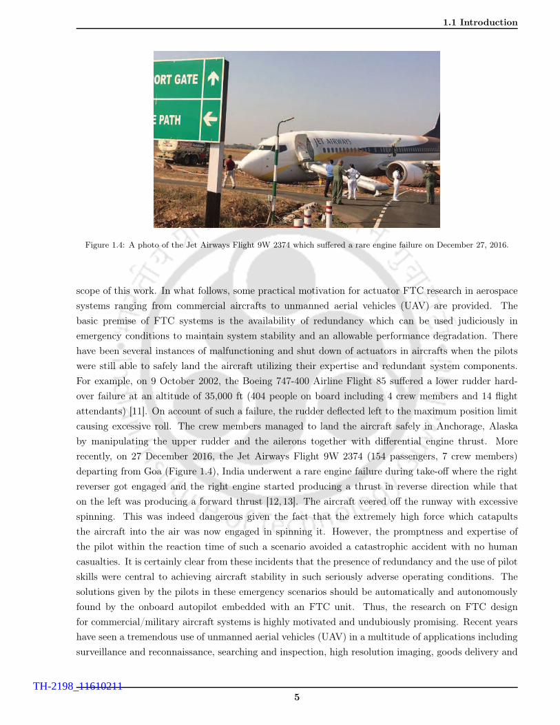
1.4 A photo of the Jet Airways Flight 9W 2374 which suffered a rare engine failure on
December 27, 2016. . . . . . . . . . . . . . . . . . . . . . . . . . . . . . . . . . . . . . . 5
1.5 Major approaches to fault tolerant control (FTC) design (adapted from [2]). . . . . . . 6
1.6 Schematic block diagrammatic representation of active fault tolerant control (AFTC)
architecture. . . . . . . . . . . . . . . . . . . . . . . . . . . . . . . . . . . . . . . . . . . 8
1.7 An event-driven interpretation and illustration of active fault tolerant control (AFTC)
architecture [3]. . . . . . . . . . . . . . . . . . . . . . . . . . . . . . . . . . . . . . . . . 8
1.8 Structure and operational flow of active fault tolerant control (AFTC) scheme adopted
in the thesis. . . . . . . . . . . . . . . . . . . . . . . . . . . . . . . . . . . . . . . . . . 9
1.9 An event-driven interpretation and illustration of active fault tolerant control (AFTC)
scheme adopted in the thesis. . . . . . . . . . . . . . . . . . . . . . . . . . . . . . . . . 9
2.1 Schematic representation the proposed fault tolerant control scheme . . . . . . . . . . 31
2.2 Visualization of the calculated invariant sets with the proposed scheme, for systems with
relative degree ℘ = 2 . . . . . . . . . . . . . . . . . . . . . . . . . . . . . . . . . . . . . 37
2.3 Plant response and control inputs under the considered fault scenario (2.79) using the
proposed control scheme. (a) Output tracking error comparison of the proposed con-
troller (red) with ASMC (blue) [4] and ABSC (green) [5]; (b) Pitch angle θ tracking
using the proposed ARFTC; (c) Pitch rate q under the proposed ARFTC; (d) Control
inputs u1 and u2 corresponding to proposed ARFTC; (e) Control inputs u1 and u2 using
ASMC [4]; (f) Control inputs u1 and u2 using ABSC procedure [5]. . . . . . . . . . . . 44
3.1 Schematic block diagram representation of a basic MMAC scheme with switching and
tuning . . . . . . . . . . . . . . . . . . . . . . . . . . . . . . . . . . . . . . . . . . . . . 49
3.2 Bidirectional robustness interactions transformed to unidirectional interaction under the
proposed FTC strategy . . . . . . . . . . . . . . . . . . . . . . . . . . . . . . . . . . . . 50
3.3 Block diagrammatic representation of the proposed adaptive fault tolerant control scheme
(AMMFTC). . . . . . . . . . . . . . . . . . . . . . . . . . . . . . . . . . . . . . . . . . 62
xiiTH-2198_11610211

List of Figures
3.4 Illustration explaining the interdependence between ‖z‖∞, controller gain parameters
and actuator failure transit time T ∗ . . . . . . . . . . . . . . . . . . . . . . . . . . . . . 77
3.5 Comparison of start-up output transient performance and parameter convergence ob-
tained with Modular Backstepping Control (MBSC) [6], single model adaptive control
and proposed multiple model adaptive control . . . . . . . . . . . . . . . . . . . . . . . 83
3.6 System states and control input with no actuator fault under Scenario 1 (3.126) from
t = 0 ∼ 50 s. (a) Output state ξ2 = x1;(b) state ξ1;(c) state ξ3 = x2; (d) control inputs
u1 and u2 . . . . . . . . . . . . . . . . . . . . . . . . . . . . . . . . . . . . . . . . . . . 84
3.7 Scenario 1. Comparison of post-failure output transient performance and parameter
convergence obtained with Modular Backstepping Control (MBSC) [6], single model
adaptive control and proposed multiple model adaptive control . . . . . . . . . . . . . 85
3.8 System states and control inputs with actuator fault under Scenario 1 (3.126) at t = 50
s. (a) Output state ξ2 = x1;(b) state ξ1;(c) state ξ3 = x2; (d) control inputs u1 and u2 86
3.9 Comparison of post failure transient performance obtained with Modular Backstepping
Control (MBSC), single model adaptive control and proposed multiple model adaptive
control in case of infinite actuator failures . . . . . . . . . . . . . . . . . . . . . . . . . 87
3.10 System states and control inputs with intermittent actuator fault/failures under Scenario
2 (3.127). (a) Output state ξ2 = x1;(b) state ξ1;(c) state ξ3 = x2; (d) control inputs u1
and u2 . . . . . . . . . . . . . . . . . . . . . . . . . . . . . . . . . . . . . . . . . . . . . 88
3.11 Comparison of start up and post failure transient performance obtained with Modu-
lar Backstepping Control (MBSC), single model adaptive control and multiple model
adaptive control in case of infinite actuator failures . . . . . . . . . . . . . . . . . . . . 89
3.12 (a) aircraft pitch angle tracking error;(b) actual and desired aircraft pitch angle θ = x3;
(c) aircraft pitch rate x4; (d) control inputs u1 and u2; . . . . . . . . . . . . . . . . . . 90
3.13 Schematic diagram of a coupled mass-spring-damper system . . . . . . . . . . . . . . . 114
3.14 (a) Tracking error comparison in displacement output y1;(b) Tracking error comparison
in displacement output y2; using the proposed adaptive FTC using multiple models and
under a single model adaptive FTC strategy. . . . . . . . . . . . . . . . . . . . . . . . 116
3.15 (a) Time evolution of y1(t) under the proposed adaptive FTC using multiple models;(b)
Time evolution of y2(t) under the proposed adaptive FTC using multiple models;(c)
Control inputs u1 and u2 under the proposed FTC scheme using multiple models; (d)
Control inputs u1 and u2 under adaptive FTC scheme using a single model. . . . . . . 117
3.16 (a) The experimental setup of a twin rotor MIMO system (TRMS) emulating a 2-DOF
helicopter; (b) Schematic physical description of the twin rotor MIMO system (TRMS). 118
3.17 Schematic of cross-coupled twin rotor MIMO system or a 2-DOF helicopter for control
development . . . . . . . . . . . . . . . . . . . . . . . . . . . . . . . . . . . . . . . . . . 119
3.18 (a) pitch and yaw angle tracking error (rad) ; (b) pitch angle θv = x1(rad); (c) yaw
angle θh = x3(rad); (d) control input voltages uv and uh (V). . . . . . . . . . . . . . . 124
3.19 (a) pitch and yaw angle tracking error (rad) ; (b) pitch angle θv = x1(rad); (c) yaw
angle θh = x3(rad); (d) control input voltages uv and uh (V). . . . . . . . . . . . . . . 125
xiiiTH-2198_11610211

List of Figures
4.1 Block diagrammatic representation of the proposed FTAC strategy . . . . . . . . . . . 148
4.2 (Left) Comparison of parameter estimation performance; (Right) Comparison of start
up transient performance; obtained with AMMFTC, Modular Backstepping Control
(MBSC) and proposed FTAC method under no failure from t = 0s− 25s. . . . . . . . 160
4.3 (Left) Comparison of parameter estimation performance; (Right) Comparison of post
failure transient and steady state performance; obtained with AMMFTC, Modular
Backstepping Control (MBSC) and proposed FTAC method under no failure from
t = 50s − 100s. . . . . . . . . . . . . . . . . . . . . . . . . . . . . . . . . . . . . . . . . 161
4.4 System states and control inputs with actuator fault under Case 1 (4.117) at t = 50 s.
(a) Output state ξ2 = x1;(b) state ξ1;(c) state ξ3 = x2; (d) control inputs u1 and u2 . . 162
4.5 Comparison of tracking performance under infinite actuator failures Case 2 (4.118) show-
ing performance improvement with increasing T ∗; (Left) tracking error performance for
T ∗ = 5s; (Right) tracking error performance for T ∗ = 15s; between Modular Backstep-
ping Control (MBSC) [6], Multiple Model (AMMFTC) and FTAC method in case of
infinite actuator failures . . . . . . . . . . . . . . . . . . . . . . . . . . . . . . . . . . . 163
4.6 System states and control inputs for Case 2 (4.118) with T ∗ = 5s. (a) Output state
ξ2 = x1;(b) state ξ1;(c) state ξ3 = x2; (d) control inputs u1 and u2 . . . . . . . . . . . 164
4.7 (a) Tracking error comparison in displacement output y1;(b) Tracking error comparison
in displacement output y2; under the action of the proposed FTAC based FTC strategy
and AMMFTC . . . . . . . . . . . . . . . . . . . . . . . . . . . . . . . . . . . . . . . . 182
4.8 (a) Time evolution of y1(t) under the proposed adaptive FTC using FTAC;(b) Time
evolution of y2(t) under the proposed adaptive FTC using FTAC;(c) Control inputs u1
and u2 under the proposed FTC scheme using FTAC; (d) Control inputs u1 and u2
under AMMFTC. . . . . . . . . . . . . . . . . . . . . . . . . . . . . . . . . . . . . . . . 183
4.9 (a) Time evolution of the pitch angle θv = x1 (rad) tracking the reference signal yr,1;(b)
Time evolution of the yaw angle θh = x3 (rad) tracking the reference signal yr,2. . . . . 185
4.10 (a) pitch and yaw tracking error (rad); (b) control input voltages uv and uh for the main
rotor and the tail rotor. . . . . . . . . . . . . . . . . . . . . . . . . . . . . . . . . . . . 186
5.1 Bidirectional robustness interactions transformed to unidirectional interaction under the
proposed FTC strategy . . . . . . . . . . . . . . . . . . . . . . . . . . . . . . . . . . . . 198
5.2 Illustration of the trajectory starting from (z(0), κ(0)) ∈ Ω(z,κ) and σ(0) /∈ Nσ converges
into (z, κ, σ) ∈ M(z,κ) ×Nσ. . . . . . . . . . . . . . . . . . . . . . . . . . . . . . . . . . 201
5.3 Time evolution of z(t) and κ(t) starting in Ω(z,κ) traversing through the set M(z,κ) and
ultimately exponentially asymptotically converging to origin. The radius k defines the
decaying exponential envelope along which z(t) converges to the origin with k → 0 as
t→ ∞. . . . . . . . . . . . . . . . . . . . . . . . . . . . . . . . . . . . . . . . . . . . . 210
xivTH-2198_11610211

List of Figures
5.4 Scenario 1: System response with the proposed fault tolerant control scheme with T ∗=
10s. (a) Comparison of output pitch angle tracking error z1 = x3−yr using the proposed
controller and modular backstepping control (MBSC) [6], (b) Pitch angle x3 = θ using
the proposed FTC scheme, (c) Pitch rate x4 = q using the proposed FTC, (d) The
estimate of the lumped uncertainty ˆ∆2 incurred due to actuator faults/failures and
modeling uncertainties, (e) Proposed control inputs u1(t) and u2(t), (f) Control inputs
u1(t) and u2(t) using modular backstepping control based FTC proposed by Wang &
Wen [6] . . . . . . . . . . . . . . . . . . . . . . . . . . . . . . . . . . . . . . . . . . . . 212
5.5 Scenario 2: System response with the proposed fault tolerant control scheme with T ∗=
10s. (a) Comparison of output pitch angle tracking error z1 = x3−yr using the proposed
controller and modular backstepping control (MBSC) [6], (b) Pitch angle x3 = θ using
the proposed FTC scheme, (c) Pitch rate x4 = q using the proposed FTC, (d) The
estimate of the lumped uncertainty ˆ∆2 incurred due to actuator faults/failures and
modeling uncertainties, (e) Proposed control inputs u1(t) and u2(t), (f) Control inputs
u1(t) and u2(t) using modular backstepping control based FTC proposed by Wang &
Wen [6] . . . . . . . . . . . . . . . . . . . . . . . . . . . . . . . . . . . . . . . . . . . . 213
5.6 Scenario 3: System response with the proposed fault tolerant control scheme. (a) Pitch
angle x3 = θ using the proposed FTC scheme, (b) Pitch rate x4 = q using the pro-
posed FTC, (c) The estimate of the lumped uncertainty ˆ∆2 incurred due to actuator
faults/failures and modeling uncertainties, (d) Proposed control inputs u1(t) and u2(t) 214
A.1 Illustration of convex sets . . . . . . . . . . . . . . . . . . . . . . . . . . . . . . . . . . 225
A.2 Illustration of construction of convex hull in the parameter space for estimating a pa-
rameter of dimension N = 1, 2, 3 (from left to right). . . . . . . . . . . . . . . . . . . . 226
xvTH-2198_11610211

List of Tables
2.1 Aircraft model parameters . . . . . . . . . . . . . . . . . . . . . . . . . . . . . . . . . . 40
2.2 Values of aircraft parameters in simulation . . . . . . . . . . . . . . . . . . . . . . . . . 40
2.3 Post failure tracking performance with 70% loss of effectiveness of u1 at t = 20s and
stuck failure of u2 at t = 40s . . . . . . . . . . . . . . . . . . . . . . . . . . . . . . . . . 45
3.1 Tabular comparison of output and input performance under Scenario 1 (3.126). . . . . 83
3.2 Tabular comparison of output and input performance for Scenario 2 (3.127) describing
infinite actuator failures with T ∗ = 5 s and T ∗ = 15 s . . . . . . . . . . . . . . . . . . . 85
3.3 Tabular comparison of output and input performances under proposed AMMFTC and
adaptive FTC using a single identification model . . . . . . . . . . . . . . . . . . . . . 116
3.4 Physical parameters of the TRMS . . . . . . . . . . . . . . . . . . . . . . . . . . . . . . 121
3.5 Tabulation of input and output performances quantified using suitable performance
measures . . . . . . . . . . . . . . . . . . . . . . . . . . . . . . . . . . . . . . . . . . . . 123
4.1 Tabular comparison of output and input performance under Case 1 (4.117). . . . . . . 161
4.2 Case 2: Performance Comparison between three adaptive control schemes, namely, finite
time adaptation based control (FTAC), adaptive control using multiple models, single
model adaptive control and modular backstepping control (MBSC) [6] . . . . . . . . . 163
4.3 Tabular comparison of output and input performances under proposed FTC under finite
time adaptation based control (FTAC), AMMFTC and adaptive FTC using a single
identification model . . . . . . . . . . . . . . . . . . . . . . . . . . . . . . . . . . . . . . 183
4.4 Tabulation of output and input performances using the proposed FTAC methodology
when applied to attitude tracking problem of TRMS. . . . . . . . . . . . . . . . . . . . 187
xviTH-2198_11610211

List of Acronyms
ABSC Adaptive backstepping control
ADRC Active disturbance rejection control
ADSC Adaptive dynamic surface control
AMMFTC Adaptive multiple model fault tolerant control
ARFTC Adaptive robust fault tolerant control
ARC Adaptive robust control
ASMC Adaptive sliding mode control
BIBS Bounded input bounded state stable
CE Certainty equivalence
CMMAC Combined multiple model adaptive control
DOB Disturbance observer
DOF Degrees of freedom
EKF Extended Kalman filter
FDD Fault detection and diagnosis
FDI Fault detection and isolation
FE Fault/Failure estimation
FTAC Finite time adaptation based control
FTC Fault tolerant control
HOSMC Higher order sliding mode control
IAE Integral absolute error
IE Initial excitation
ISMC Integral sliding mode control
ITAE Integral time absolute error
LIP Lock in place
LMI Linear matrix inequality
MBSC Modular backstepping control
MIMO Multiple input multiple output
MISO Multiple input single output
MMAC Multiple model adaptive control
NDOB Nonlinear disturbance observer
PCI Peripheral component interconnect
PE Persistenly exciting
xviiTH-2198_11610211

List of Acronyms
PLF Piecewise Lyapunov function
PLOE Partial loss of effectiveness
PPB Prescribed performance bound
RMSE Root mean square error
SMC Sliding mode control
SOSM Second order sliding mode
TLOE Total loss of effectiveness
TRMS Twin rotor MIMO system
TV Total variation
UUB Uniformly ultimately bounded
xviiiTH-2198_11610211

List of Symbols
:= defined as
, by definition
⊂ proper subset of
⊃ proper superset of
⊆ subset of
⊇ superset of
∀ for all
∩ intersection
(·)† pseudo inverse of the argument
∈ belongs to
∋ does not belong to
∃ there exists
designating the completion of proofs
→ tends to
=⇒ implies that
R the space of real numbers
R+ the space of positive real numbers
Rn the space of real valued vectors of dimension n
Rm×n the space of real valued m× n matrices
W the set of whole numbers
N the set of natural numbers
2N the set of all even numbers
N/2N the set of all odd numbers
Z+ the set of positive integers
| · | absolute value of a scalar argument
(·)T transpose of the argument (vector or matrix)
‖A‖∞ induced ∞−norm of a matrix
‖A‖F the Frobenius norm of the matrix A
max· the maximum of the arguments
min· the minimum of the arguments
sup the least upper bound
TrA the trace of the matrix A
xixTH-2198_11610211

List of Symbols
det(A) the determinant of matrix A
f : S1 → S2 a function f mapping space S1 onto space S2
7→ maps to
‖ · ‖p Lp norm for p ∈ [1,∞) of the argument vector
‖ · ‖∞ L∞ norm of the argument vector
(·) upper bound of the argument
(·) lower bound of the argument
L1[a, b] the signal space L1[a, b] = x(t) ∈ Rn | ‖x‖1 <∞ for t ∈ [a, b]
L2[a, b] the signal space L2[a, b] = x(t) ∈ Rn | ‖x‖2 <∞ for t ∈ [a, b]
L∞[a, b] the signal space L∞[a, b] = x(t) ∈ Rn | ‖x‖∞ <∞ for t ∈ [a, b]
L1 the signal space L1 = x(t) ∈ Rn | ‖x‖1 <∞ for t ∈ [0,∞)
L2 the signal space L2 = x(t) ∈ Rn | ‖x‖2 <∞ for t ∈ [0,∞)
L∞ the signal space L∞ = x(t) ∈ Rn | ‖x‖∞ <∞ for t ∈ [0,∞)
y, y first and second derivative of y with respect to time
y(i) the ith time derivative of y with respect to time
λ(·) maximum eigen value of the matrix argument
λ(·) minimum eigen value of the matrix argument
A/B quotient operation between two sets A and B, i.e., A−B
A×B the cartesian product between two sets
diaga1, . . . , an an n× n diagonal matrix with diagonal elements a1 to an
Lf (·) the Lie derivative along the direction of vector field f
In or In the identity matrix of dimension n× n
m, q, p dimension of system input, output and unknown parameter vector
Proj(·) the projection operator
℘ the relative degree of a system
℘i the relative degree of ith subsystem
sign(x) the signum function such that sign(x) is 1, 0 or -1
respectively, according as x > 0, x = 0, x < 0
δ(t − a) the impulse function defined at t = a
U(t− a) the unit step function defined at t = a
Mp% the percentage of peak overshoot
Mu% the percentage of peak undershoot
xxTH-2198_11610211

List of Publications
International Refereed Journals
1. A. Chakravarty and C. Mahanta, “Actuator fault-tolerant control (FTC) design with post-faulttransient improvement for application to aircraft control”, International Journal of Robust andNonlinear Control, Wiley, vol. 26(10), pp. 2049-2074, 2016.
Manuscript Under Preparation
1. A. Chakravarty, I. Kar and C. Mahanta, “A new interacting multiple model adaptive controlapproach to compensate infinite actuator failures in nonlinear uncertain systems: stability, con-vergence and performance”, IEEE Transactions on Automatic Control, Draft prepared to besubmitted.
2. A. Chakravarty and C. Mahanta, “Enhanced Parameter convergence and output performanceimprovement via a novel finite time adaptation based fault tolerant controller for nonlinear un-certain systems”, Automatica, Draft prepared to be submitted.
3. A. Chakravarty, C. Mahanta and I. Kar, “Adaptive compensation of parametrization-free infiniteactuator failures in nonlinear uncertain systems with finite time performance recovery”, IEEETransactions on Automatic Control, Draft prepared to be submitted.
4. A. Chakravarty, C. Mahanta and K. S. Amezquita, “Adaptive compensation of actuator failuresin MIMO nonlinear uncertain systems with finite time fault estimation and improved transientperformance applied to aircraft control", IEEE Control Systems Letters, To submit.
Conference Proceedings
1. A. Chakravarty, T. K. Nizami, I. Kar and C. Mahanta, “Adaptive compensation of actuatorfailures using multiple models”, 20th IFAC World Congress, Vol 50, No. 1, Toulouse, France,2017, pp. 10350-10356.
2. A. Chakravarty and C. Mahanta, “Compensating actuator failures in near space vehicles usingadaptive finite time disturbance observer based backstepping controller”, Proc. of 2016 EuropeanControl Conference (ECC), Aalborg, Denmark, 2016, pp. 98-103.
3. A. Chakravarty and C. Mahanta, “Finite time actuator failure compensation of near space vehiclesusing an observer based backstepping method”, Proc. of LAMSYS-2016, Satish Dhawan SpaceCentre, Sriharikota, ISRO, India, 2016.
4. A. Chakravarty and C. Mahanta, “Backstepping enhanced adaptive second order sliding modecontroller to compensate actuator failures”, Proc. of 2014 Annual IEEE India Conference (IN-DICON), Pune, India, 2014, pp. 1-6.
xxiTH-2198_11610211

List of Publications
5. A. Chakravarty and C. Mahanta,“Actuator fault tolerant control scheme for nonlinear uncertainsystems using backstepping based sliding mode”, Proc. of 2013 Annual IEEE India Conference(INDICON), Mumbai, India, 2013, pp. 1-6.
xxiiTH-2198_11610211

1Introduction
Contents
1.1 Introduction . . . . . . . . . . . . . . . . . . . . . . . . . . . . . . . . . . . . . 2
1.2 Literature Review . . . . . . . . . . . . . . . . . . . . . . . . . . . . . . . . . . 10
1.3 Research Motivation . . . . . . . . . . . . . . . . . . . . . . . . . . . . . . . . 14
1.4 Contributions of the Thesis . . . . . . . . . . . . . . . . . . . . . . . . . . . . 17
1.5 Thesis Organization . . . . . . . . . . . . . . . . . . . . . . . . . . . . . . . . . 19
1TH-2198_11610211

1. Introduction
1.1 Introduction
Control theory plays an integral role in deciding the behavior of all dynamical systems existing in
nature. The concept of feedback is central to almost all control systems and has indeed been instrumen-
tal in acheiving system output regulation or desired reference trajectory tracking. With overwhelming
technological developments and spectacular success of the industrial revolution, the early 19th century
witnessed the first instances of feedback control systems in the form of Watt’s centrifugal governor
shown in Figure 1.1 [1]. The centrifugal governor was intended to control the output shaft speed of the
steam engine. Until 1868, the design of control systems in such mechanical and electrical machineries,
was primarily an art procured from intuition, experience and engineering ingenuity. Such approaches
abstained from representing the control problem, its objectives and imposed constraints in terms of
mathematical relationships. As a result, these ad hoc control solutions failed to provide analytical
Figure 1.1: Centrifugal governor [1]
insights into system behavior in the event of parameter variations and unanticipated disturbances;
and hence attaining a robust and optimized performance was certainly questionable. By then, a for-
mal mathematical analysis had already begun with the study of governor dynamics by physicist J.C.
Maxwell [1]. Eventually, the analysis led to the introductory concept of limit cycle oscillations and
the fundamental notion of instability in dynamical systems under feedback. In consequence, these
issues motivated several analytical developments regarding dynamic instability of linear systems in the
West; the most remarkable one being the celebrated Routh-Hurwitz stability criterion. Alternatively,
one of the greatest developments in the theory of stability of dynamic systems was the publication of
Lyapunov’s famous memoir in 1892 followed by promising methods on stability analysis. By World
War II, owing to demands of high performance and stability of closed-loop feedback control systems,
mathematical research on automatic control theory gained enough impetus for applications in missile
guidance and control, ship steering, and aircrafts. Servomechanisms in frequency domain were de-
2TH-2198_11610211

1.1 Introduction
signed from theoretical results on dynamic stability using frequency response, bandwidth, gain and
phase margins. Restricted to linear systems, these methods lacked severely in achieving performance
robustness and resulted in a very limited dynamically stabilizable operating regime. In contrary, the
stability results independently proposed by Lyapunov in the Soviet Union, was more general and was
applicable to systems regardless of their input-output characteristics. These results were indeed a ma-
jor scientific breakthrough for the Soviet Union which marked the emergence of modern control theory
and the inception of new control paradigms based on state space approaches.
1.1.1 Fault Tolerant Control
Apart from stability; safety, reliability and performance are among the essential operational charac-
teristics sought for in control of dynamical systems, especially in mission critical applications. Besides,
cost effectiveness has also been an added design objective to be possibly met. Imperfections in system
modeling, uncertain operating environment, large variations in parameters, malfunctioning or dam-
age of system components further complicate the synthesis of a stable controller. On similar lines,
it is extremely difficult to ensure the existence of sustainable closed-loop system solutions respecting
the foregoing design attributes using conventional feedback control. Consistent attempt to address
these design challenges gradually motivated the development of retrofit control technologies for com-
plex safety critical systems to render resilience to uncertain eventualities. In this direction, the first
pioneering effort was the launch of Self Repairing Flight Control System Program [7] by the US Air
Force in 1984. Eventually followed up by the National Aeronautics and Space Administration (NASA),
this initiative led to the inception of a new research avenue in the field of control theory applications
known as fault tolerant control (FTC) [8]. Hence, FTC systems are defined as control systems that are
equipped with the ability to accommodate system, component faults or failures automatically and are
capable of maintaining overall system stability and acceptable performance in the event of such fault or
failure [8–10].
Fault can be defined as an undesired change in a system parameter that degrades performance.
Whereas, failure is an eventuality that results in catastrophic or complete breakdown of a component
or function which can be compared to a fault which is a tolerable malfunction. Having defined the
terminologies, a broad classification comprises of actuator, sensor and system faults/failures. Changes
in operating points, large uncertain abrupt variation in system parameters, payload variations, etc.
are termed as system faults. On the other hand, sensor faults manifest themselves in incorrect mea-
surements with noise, measurement bias, freezing and drift. Actuator faults/failures and their types
are illustrated in Figure 1.2. The variable tf denotes the failure instant and umax, umin are the maxi-
mum/minimum limits of actuation magnitude. Different types of actuator failures are demonstrated
using an aircraft example. Figure 1.3 shows a commercial aircraft exhibiting faults and failures in
ailerons (fal), elevators (fe) and rudder (fr). Faults in such control surfaces occur in the form of par-
tial loss of effectiveness (PLOE) as shown in Figure 1.2(d), wherein the actuator operates with reduced
efficiency after time tf . Total actuator failures manifests in three forms, namely, float, lock-in-place
(LIP) and hard-over failures (Figure 1.2(a)-(c)). Float failure is a condition when the control surface
moves freely and has no moment contribution to the aircraft. While LIP failure results in the condition
3TH-2198_11610211

1. Introduction
where the actuator is stuck or jammed at a certain value. The most catastrophic form of actuator
failure is the hard-over failure where the actuator actuates at its maximum rate limit until its position
reaches the blowdown limit.
umax
umax umax
umax
umin umin
uminumin
0 0
0 0
Time Time
Time Time
t f t f
t f t f
(a) Float Failure (b) Lock-in-place
(c) Hard over (d) Loss of Effectiveness
Desired Actuator output Faulty Actuator output
Figure 1.2: Illustration of the types of actuator faults and failures in dynamical systems.
Figure 1.3: Demonstration of actuator faults and failures of control surfaces in Boeing 747 aircraft.
This thesis broadly concerns the design, development and analysis of fault tolerant controllers to
compensate actuator faults and failures in addition to system uncertainties and external disturbances.
The generalized problem of FTC has not been attempted and hence sensor failures are beyond the
4TH-2198_11610211
1.1 Introduction
Figure 1.4: A photo of the Jet Airways Flight 9W 2374 which suffered a rare engine failure on December 27, 2016.
scope of this work. In what follows, some practical motivation for actuator FTC research in aerospace
systems ranging from commercial aircrafts to unmanned aerial vehicles (UAV) are provided. The
basic premise of FTC systems is the availability of redundancy which can be used judiciously in
emergency conditions to maintain system stability and an allowable performance degradation. There
have been several instances of malfunctioning and shut down of actuators in aircrafts when the pilots
were still able to safely land the aircraft utilizing their expertise and redundant system components.
For example, on 9 October 2002, the Boeing 747-400 Airline Flight 85 suffered a lower rudder hard-
over failure at an altitude of 35,000 ft (404 people on board including 4 crew members and 14 flight
attendants) [11]. On account of such a failure, the rudder deflected left to the maximum position limit
causing excessive roll. The crew members managed to land the aircraft safely in Anchorage, Alaska
by manipulating the upper rudder and the ailerons together with differential engine thrust. More
recently, on 27 December 2016, the Jet Airways Flight 9W 2374 (154 passengers, 7 crew members)
departing from Goa (Figure 1.4), India underwent a rare engine failure during take-off where the right
reverser got engaged and the right engine started producing a thrust in reverse direction while that
on the left was producing a forward thrust [12, 13]. The aircraft veered off the runway with excessive
spinning. This was indeed dangerous given the fact that the extremely high force which catapults
the aircraft into the air was now engaged in spinning it. However, the promptness and expertise of
the pilot within the reaction time of such a scenario avoided a catastrophic accident with no human
casualties. It is certainly clear from these incidents that the presence of redundancy and the use of pilot
skills were central to achieving aircraft stability in such seriously adverse operating conditions. The
solutions given by the pilots in these emergency scenarios should be automatically and autonomously
found by the onboard autopilot embedded with an FTC unit. Thus, the research on FTC design
for commercial/military aircraft systems is highly motivated and undubiously promising. Recent years
have seen a tremendous use of unmanned aerial vehicles (UAV) in a multitude of applications including
surveillance and reconnaissance, searching and inspection, high resolution imaging, goods delivery and
5TH-2198_11610211

1. Introduction
in-flight refueling and various military missions. Therefore, their relentless deployment in fire-fighting
and surveillance operations largely under rough environmental conditions including natural disasters,
make them highly vulnerable to on-flight actuator failures. Of late, in this regard, the Washington
Post has reported more than 400 crashes of military UAVs in the United States since 2001 [14, 15].
Besides mission failures, these crashes have led to huge loss of property including but not limited
to, destruction of houses, farms, forest fires, airport and naval base infrastructures, etc, which is also
unfortunate. Indeed, with years of rapid technological advancements in the 21st century, new inventions
of mechanical/aerospace systems and their multifaceted applications have come up with several design
and operational issues including reliability and safety. Thus, from a control design perspective, these
burgeoning issues and their subsequent challenges leave a exciting aura for further research on actuator
FTC synthesis for dynamical systems.
1.1.1.1 Approaches to FTC Design
Approaches to FTC design are broadly classified into two categories, namely, an active and a
passive approach. Figure 1.5 depicts the classification of FTC along with the segregation between
various important control methodologies as active and passive methods.
Fault Tolerant Control
Passive
RobustControl
Sliding ModeControl (SMC)
H Infinity
Integral SlidingMode Control
(ISMC)
(FTC)
AdaptationControl SignalRedistribution
MultipleModels
Scheduling Prediction
ControlAllocation
DynamicInversion
Multiple Model
Switching and Tuning (MMST)
Interacting
(IMM)
GainScheduling
Linear ParameterVarying(LPV)
Model Predictive
Active
Control
Multiple Models
Model Reference
Adaptive Control(MRAC)
Self Tuning Control (STC) (DI)
(CA) (GS)(MPC)
Figure 1.5: Major approaches to fault tolerant control (FTC) design (adapted from [2]).
Active fault tolerant controllers are online self repairing strategies which rely on three fundamental
units, namely, an fault detection and isolation (FDI) unit, a reconfigurable controller and a control
reconfiguration mechanism to achieve fault tolerance and nominal performance recovery. A schematic
6TH-2198_11610211

1.1 Introduction
block diagram representing the basic design structure of active FTC is shown in Figure 1.6. These three
units have to work in a cooperative manner to guarantee system stability and optimal excellent output
performance in the event of a failure. The illustration in Figure 1.7 shows the operational procedure of
an active FTC scheme from an event-driven perspective sarting from the occurence of a fault/failure
until it is recovered. The operation modes of the system are denoted by H (healthy/faultfree), F
(faulty), D (fault diagnosed) and R (reconfigured). The terms Ef , Ed, Erc and Er denote the events
resulting in the transition from one operational mode to the other. The explanation of an active FTC
scheme based on FDI is as follows: The controller starts to operate in H (faultfree) operation mode.
Due to occurrence of a fault/failure event Ef , the control system transits from H mode to F(faulty)
mode. Thereafter, from the diagnosis event Ed and mode D, the reconfiguration event Erc enables
the system to attain a desirable reconfiguration mode (R) where it should be at least stable and
should satisfy the design objectives as much as possible. Following the synthesis of the reconfigurable
controller, a suitable reconfiguration strategy is designed to make the system transit to its (H) healthy
mode through the recovery event Er. The timing diagram in Figure 1.7(right) shows the temporal
relation between the events incurred within this active FTC architecture. Although appearing to be
apparently advantageous, it exhibits the following shortcomings: (a) The success of fault tolerance
solely depends on the correctness of the FDI unit. However, guaranteeing robustness FDI results to
modeling uncertainties is difficult and hence false alarms are often incurred. This eventually leads to
incorrect reconfiguration thereby degrading performance and at times may destabilize the system; (b)
In safety critical systems, where time is a crucial parameter, there is a time interval within which the
active FTC system should detect the fault and subsequently resort to reconfiguration and FTC action.
This time is known as the critical reaction time. Therefore, as shown in the timing diagram in Figure
1.7(right) if the time delay incurred in fault diagnosis Ed until reconfiguration Erc is greater than the
critical reaction time, the fault/failure is not recoverable and the system experiences instability which
is undesirable; (c) Further, the switching action (reconfiguration) between optimal control solutions
aligned to each type of faults/failures based on a reconfiguration criterion results in harmful switching
transients. These transients contribute to sabotage the fault tolerant performance of the active FTC
system. Further, closed loop instability can occur in case the system considered does not have a
positive dwell time; (d) The reconfiguration procedure involves a complex decision making process
which is computationally intense. The reconfiguration time adds to the computation time of the
reconfiguration solution which increases with the growing dimension of the system. All these factors
inhibit a successful implementation of an integrated FDI based FTC system.
Owing to practical implementation challenges of an integrated FDI based FTC design, an integrated
fault estimation(FE) based FTC emerges to be a promising alternative. The basic architecture of an FE
based FTC system is illustrated in the block diagram presented in Figure 1.8. Similar to the explanation
of an FDI based FTC, to elucidate the working of an FE/FTC strategy, an event driven architecture of
the same is depicted as a finite state automaton in Figure 1.9. Such a FTC design topology comprises of
three operation modes and three events to allow transition between each of the modes. The operation
modes are denoted by H (healthy/faultfree), F (faulty) and E(fault estimated) while the events are
represented as Ef , Ee and Er defining the occurrence of fault, fault estimation and failure recovery,
7TH-2198_11610211

1. Introduction
Figure 1.6: Schematic block diagrammatic representation of active fault tolerant control (AFTC) architecture.
Ef
Ed Erc
Er
H
F
D
R
Ef Ed Erc
Eve
nts
tDiagnosis delay
Reconfiguration time
(a) (b)
Figure 1.7: An event-driven interpretation and illustration of active fault tolerant control (AFTC) architecture [3].
8TH-2198_11610211

1.1 Introduction
respectively. This design framework does not rely on any switching or reconfiguration strategy and
controller reconfiguration. It consists of a single controller wherein the fault estimation from the FE
module can be retrofitted to achieve fault tolerance and improved output performance. Hence, the
design is indeed computationally appealing with increased design freedom and has great potential for
practical use in FTC applications. Besides, closed loop stability analysis of the integrated FE/FTC
scheme is comparatively tractable. Apart from the aforementioned advantages, system performance
recovery cannot be guaranteed if the critical reaction time is lesser than the time required for fault
estimation. Several active FTC methodologies have been proposed in literature using model reference
adaptive control [16, 17], self tuning [18], control allocation [19–21], multiple models [22–24], gain
scheduling [25], linear-parameter varying approaches [26], model predictive control [27, 28], adaptive
sliding mode control [4, 29, 30], adaptive backstepping control [5, 31, 32].
[33] On the other hand, passive FTC schemes are off-line strategies based on robust control ideas
Figure 1.8: Structure and operational flow of active fault tolerant control (AFTC) scheme adopted in the thesis.
Ef Er
Ee
H
F E
Ef Ee
Eve
nts
tEstimation time
(a) (b)
Figure 1.9: An event-driven interpretation and illustration of active fault tolerant control (AFTC) scheme adopted inthe thesis.
and do not require any online scheme of fault detection and diagnosis. A single fixed controller is
9TH-2198_11610211

1. Introduction
designed by considering a predetermined set of faults and failures that can probably occur, during
the design stage. The fundamental objective of passive FTC methods is to maintain stability of the
system in the event of multiple failures without striving for optimal performance corresponding to any
specific fault. Therefore, any passive FTC design is conservative in terms of performance and hence
not suitable for performance critical systems. Passive FTC basically makes a trade-off between system
performance and stability. Further, since most passive FTC designs are formulated as optimization
problems, it is very likely to encounter ill posed problems wherein, the existence of solutions is not
guaranteed. Hence, performance robustness of passive schemes are limited to a restrictive repertoire
of anticipated actuator failures. Various passive FTC methodologies have been proposed in literature,
for instance, H∞ control [34–39], sliding mode control (SMC) [40–42] and integral sliding mode control
(ISMC) [43,44].
This thesis adopts an active FTC approach to guarantee robustness to large class of faults and
failures, maintain optimal performance and therefore attempts to increase its reliability and applica-
bility. In what follows, the active FTC methodologies pertaining to nonlinear uncertain systems are
reviewed.
1.2 Literature Review
The basic premise of an actuator fault tolerant control (FTC) system is to achieve fault tolerance
and maintain a stable post fault/failure output tracking by redesigning/reconfiguring the control input.
Besides, in safety and mission critical systems, owing to a large variation in operating points, the FTC
design should ensure increased stability margins and an expanded dynamically stable operating regime.
In addition, robust output performance in presence of system uncertainties and external disturbances
is another design objective in FTC. For example, in aircrafts, UAVs, spacecrafts, the wide variations
in aerodynamic coefficients, Mach, altitude, dynamic pressure, angle of attack (AoA) and payload are
inevitable. Payload variations may occur due to fuel consumption, release of missiles and carriage.
Apart from actuator failures, these factors, if not compensated, also contribute to decreased flight
envelope with degraded flying quality and may be a factor for potential instability as well. Thus,
design of an actuator failure resilient control system which automatically adapts to the change in
operating conditions and guarantees closed loop stability over its entire operating envelope, is indeed
a Herculean task. Moreover, considering the system to be nonlinear, further adds a dimension to
the difficulty of the foregoing FTC design. Aligned with the aforementioned control design problem,
different FTC strategies based on passive and active philosophies have been proposed for both linear
and nonlinear systems. However, none of the methodologies has been able enough to address the design
objectives in a unified manner. Passive FTC methodologies and their shortcomings have been reviewed
in the previous section. To be specific with the development of the thesis objectives within the ambit
of active FTC; in the following, a brief survey of relevant literature on various active FTC methods
for nonlinear dynamical systems is provided.
In the context of nonlinear systems, a number of active FTC schemes have been proposed, such as,
control allocation [45–47], neural networks/fuzzy logic based control [48–52], multiple model adaptive
10TH-2198_11610211
1.2 Literature Review
control [24, 53–56], reconfigurable control with learning [57], model predictive control [27, 28, 58], and
SMC/ISMC with control signal redistribution [59–61]. These control strategies solely rely on an FDI
based control design architecture (Figure 1.6) and hence are more likely to suffer from its inherent
drawbacks. Besides, assumption of existence of system dwell time, switching mechanism, increasing
computational burden and excessive input usage proportional to output performance; are some of
the features exhibited by the above-mentioned active FTC design. In view of these foregoing issues,
practical implementation of such schemes is difficult and hence, their applicability is largely restricted
to a specific class of nonlinear systems only.
On the other hand, adaptive control methodologies are found to be intuitively appealing in the de-
sign of efficient active fault tolerant controllers for nonlinear systems. Among all active FTC schemes,
adaptive controllers offer two major conceptual advantages. Firstly, only a single adaptive controller
is needed to compensate actuator failures. Secondly and more importantly, these controllers do not
require an explicit fault detection and diagnosis (FDD) module eluding the implementation issues of
FDD and subsequent reconfiguration in real time. This motivated the design of active fault tolerant
controllers for nonlinear systems subjected to complete actuator failures. With an aim to achieve total
failure tolerance in uncertain nonlinear systems, direct adaptive control strategies have been proposed
for multiple input single output and multiple input multiple output nonlinear uncertain systems using
adaptive feedback linearization [62–65], adaptive backstepping control (ABSC) [5,32,54] and adaptive
dynamic surface control (ADSC) methodologies [66,67]. Although, adaptive feedback linearization [68]
procedures of actuator FTC design reported in [62–65] are methodically attractive and ensure a faithful
compensation of actuator failures, the design requires an accurate and complete knowledge of system
dynamics. In real time, the presence of parametric uncertainties in system dynamics is obvious and
their adverse effects on system performance is inevitable. However, apart from actuator failures, in-
corporating compensation of uncertain system parameters into feedback linearization design leads to a
large dimension of parameter estimates. As a result, overparameterization prevails, culminating in high
computational burden and the closed loop solutions may experience numerical instability. Whereas,
ABSC [69] and ADSC [70] methodologies [5, 32, 54, 66, 67] address the issues of compensating coexist-
ing system uncertainties along with actuator failures and ensure stable fault tolerant output tracking.
However, an FTC based on ADSC does not offer asymptotic stability and its transient and steady state
performances are dependent on the chosen time constants of intermediate low pass filters encountered
in the course of design. Further, a robust adaptive output feedback controller designed using backstep-
ping procedure was developed in [71, 72] to stabilize a nonlinear system affected by uncertain linearly
parameterized actuator failures. Eventually, the results of [71,72] were extended in [73] to compensate
parameterizable as well as non-parameterizable actuator failures. The aforementioned methodologies
are reported to yield promising results in the event of uncertain actuator failures in presence of state de-
pendent matched and unmatched uncertainties only. Actuator failures in nonlinear systems with model
uncertainties, have also been compensated using adaptive sliding mode control (ASMC) [4,30,74]. With
the ASMC in action, the closed-loop system exhibits fast response and makes the system output in-
variant to actuator faults/failures. The design of ASMC is primarily based on the bound estimation
of lumped uncertainty encompassing state dependent system uncertainties, external disturbances and
11TH-2198_11610211

1. Introduction
actuator failures. Moreover, the lumped uncertainty should necessarily satisfy the matched condition.
Further, unlike [5, 32, 54, 62–67], the most severe drawback of ASMC is its discontinuity across sliding
surfaces which leads to chattering and subsequent excitation of neglected high-frequency dynamics.
To make ASMC strategies practically feasible for FTC, efforts to alleviate chattering using sigmoid
function based smoothing and boundary layer approximation have been proposed. However, the track-
ing precision is severely compromised with control smoothing. Although transient performance is still
acceptable, asymptotic stability is lost. In summary, translation of ASMC techniques from theory to
practice suffers from a trade-off between output performance and control bandwidth. Inspired by pre-
scribed performance bound (PPB) based adaptive controllers, using a variable transformation, ABSC
is designed to compensate actuator failures [31]. Such a method ensures that the output trajectory
never escapes the pre-defined exponential envelope and hence, offers a guaranteed transient and steady
state performance. Recently, a bound estimation based backstepping control approach using tuning
functions [75] is proposed for nonlinear systems with uncertainties, to compensate finite as well as
possibly infinite (intermittent) actuator failures. However, the proposed adaptive control solution and
its ultimate transient bounds explicitly depend on time. Besides, another direct adaptive backstepping
controller is proposed using a fusion of tuning function approach, nonlinear damping and a projection
based parameter adaptation [76]. The review of direct adaptive FTC approaches herein shows their
design flexibility and potential to be retrofitted into an existing control loop in complex critical systems
to ensure fault tolerance.
Indirect adaptive FTC strategies have also been proposed for nonlinear systems assuming the
presence of decoupling between the estimator-controller pair. Herein, the unknown parameters are
estimated first and then the control signal comprising of functions of these unknown parameters is
calculated using these estimates. These controllers are characterized by a poor oscillatory transient
behaviour during their learning phase. Their output performance is directly correlated to the accu-
racy and fastness of parameter estimation. Moreover, overparameterization is absent. Very few works
have been reported in adaptive FTC literature so far on deriving an indirect adaptive compensator
for linearly parametrized nonlinear systems affected by actuator failures. It is our belief that such a
cold attitude towards adopting an indirect adaptive approach for FTC design is ascribed to its poor
output transient performance. Within a certainty equivalence (CE) based indirect adaptive control
structure, introduction of large parameteric uncertainties due to actuator failures may result in high
output overshoots which may trespass the safety limits of the system. Further, to ensure modularity
between controller and the estimator, the nonlinear system should be necessarily globally Lipschitz.
Further, the closed loop stability analysis and proof of asymptotic stability is not straightforward. Al-
though substantial number of these controllers contribute to FTC literature on linear systems, solving
the failure compensation design problem using similar strategies for nonlinear systems has rarely been
considered by researchers. Lately, the problem of actuator failure compensation in nonlinear MIMO
systems with linearly parameterizable uncertainties, is attempted using a multiple model adaptive con-
trol with switching and tuning [24]. Assuming modularity of controller-identifier pair, the proposed
backstepping controller follows an indirect adaptive control design philosophy and the transient perfor-
mance is improved by the use of multiple identification models in conjunction with PPB control. The
12TH-2198_11610211
1.2 Literature Review
first seminal work on adaptive compensation of infinite actuator failures in nonlinear uncertain systems
is based on a modular adaptive backstepping control [6]. Except for switching multiple model based
adaptive control (MMAC) approaches to FTC, active FTC methods based on indirect adaptive con-
trol are based on an fault estimator (FE) based FTC architecture driven by three events and a single
controller, without any reconfiguration/switching strategy between a bank of controllers/estimators
(see Figures 1.8-1.9). With reference to FE/FTC design topology, some of the major active FTC
techniques for parametrization free system uncertainties and actuator failures are discussed below.
Based on the fault estimate from a nonlinear unknown input observer, an adaptive sliding mode fault
tolerant controller is designed [77] for Lipschitz nonlinear systems. The observer and the control gains
are obtained from solutions of an H∞ optimization problem to minimize the bidirectional robustness
interactions between the controller and the observer. In [78], differential geometric tools are utilized
to design an FE integrated FTC scheme. A neural network observer based backstepping controller is
proposed in [79] to estimate the failure pattern and magnitude for multivariable nonlinear systems.
Active disturbance rejection controllers (ADRC) using nonlinear disturbance observers (NDOB)
have recently earned great popularity due to excellent estimation and output transient performance.
They are indeed applicable to a large class of nonlinear systems owing to their capability to handle
a large class of nonlinear and linear uncertainties and disturbances. Herein, the design procedure
first assumes that the system is bounded under the action of a nominal control law. Thereafter,
a disturbance observer is designed which estimates the temporal profile of the lumped uncertainty
comprising of state dependent system uncertainties, external disturbances and parameterization free
actuator failure induced perturbations. Some of the recent works on ADRC based active actuator
failure compensators can be found in [80–83] and the references therein. These disturbance observers
(DOB) utilize the information from the disturbance prediction error and/or the state prediction error to
estimate the distubance. Subsequently, the estimated disturbance is fed back to the nominal controller
for subsequent cancellations. ADRC startegies can be categorically placed under an indirect adaptive
FTC design scheme for nonlinear systems affected by uncertainties and actuator failures which are
not necessarily parameterized. Further, adaptive neural FTC based on disturbance observers with
composite adaptation have also been proposed recently in [84–88]. These estimator based control
algorithms follow an integrated design approach where the disturbance observer utilizes the disturbance
prediction error for its estimation. Neural networks with online learning are used to estimate unknown
state dependent nonlinearities and disturbance estimation error for subsequent compensation. The
online learning herein is based on the information from either the tracking error, the state prediction
error or both. Although through proper tuning of controller gains, output transient performance is
preserved at large; asymptotic stability of the output is lost. Globally uniformly ultimately bounded
closed loop trajectories are not guaranteed. Finally, it is observed that ADRC startegies at large are
also easy to be integrated to any nominal existing control loop without changing the control structure.
Hence, with the retrofit property, DOB based adaptive control qualifies to be a potential choice for
FTC applications in real time.
13TH-2198_11610211

1. Introduction
1.3 Research Motivation
It is evident from the literature review in the preceding section that the area of active FTC design,
has been extensively researched upon. Fruitful results within the active framework have been reported
as regards control of nonlinear uncertain systems to compensate unknown actuator faults and failures.
However, there are still a number of challenging problems which are yet to be addressed. Some of the
open theoretical issues drawing our attention are discussed below.
• Control design using a direct adaptive backstepping technique is known to offer a promising
output transient performance through trajectory initialization and initial increase of the virtual
control gains. The same ideology translates analogously to transient performance improvement
in adaptive sliding mode control (ASMC) through increment in the sliding surface coefficients.
However, actuator faults and failures are unknown in time, and hence, trajectory initialization
is not so feasible. Further, it has been mathematically proved in [69] that an increase in the
virtual control gains may improve the start-up transients while such a measure will increase the
value of the tracking error at the instant of actuator fault/failure. In consequence, the post-fault
transient performance is degraded and the output experiences cumulatively high overshoots with
each instance of failures, which is undesirable. Addressing this design issue, an adaptive back-
stepping control based failure compensation is proposed in [31] guaranteeing prescribed output
transient performance in the event of complete actuator failures and PLOE faults. However,
since the design philosophy relies on the ideology of high gain adaptive controllers using perfor-
mance funnels, the control energy, in this case, varies inversely with the prescribed error bounds.
Although being theoretically promising, owing to design and physical constraints in practical
systems, rewarding application of such controllers to crucial FTC problems is doubtful and may
not be promising. Therefore, it would be interesting to develop new backstepping based adaptive
control strategies wherein the output transients in failure cases can be improved independent of
the choice of virtual control gains and trajectory initialization without any significant increase
in the control effort.
• From the perspective of active approaches, most of the active FTC schemes rely on fault detec-
tion and isolation (FDI) unit for controller reconfiguration in the event of uncertain eventualities
of actuator faults and failures. However, the performance and correctness of such residual based
FDI schemes are largely affected by system modeling errors, parametric uncertainties and exter-
nal disturbances, which may often lead to false alarms. Thus, FDI strategies strictly require an
optimal determination of residual signals and a selection of detection thresholds so as to success-
fully differentiate between an actuator failure and an uncertainty. Thereafter, a reconfiguration
strategy based on the information from FDI unit is to be formulated to conform the system with
the failure induced changes and maintain stability. Nevertheless, an integrated FDI based FTC
design is very difficult to realize and implement [89, 90], owing to a discrete event structure of
reconfiguration, time delay in FDI and optimality factors regarding modeling imperfections and
external disturbances during the detection phase. In summary, the integrated FDI/FTC design
problem essentially reduces to a hard optimization problem and finding a solution satisfying the
14TH-2198_11610211
1.3 Research Motivation
design constraints is indeed difficult, if not impossible [9, 10]. Although being apparently ad-
vantageous, the aforementioned design issues along with implementation complexity inhibits its
translation to practice, especially in systems, where safety is an overriding concern. Moreover,
the design is far more difficult for general nonlinear dynamical systems. Most of the research on
FTC conducted till date, is on model based FDI without an FTC function or on fault tolerant
control (FTC) design without the requirement of FDI module for computational simplicity.
As an alternative, an integrated fault estimator (FE) based active FTC architecture can be re-
sorted to. Such a design can be realized in either ways by adopting a direct or an indirect adaptive
control philosophy. However, FE/FTC design based on the philosophy of direct adaptive control
is believed to exhibit high and aggressive control effort since its learning is directly dependent
on the output [91]. To economize the control requirement, FE/FTC synthesis on the basis of
indirect adaptive control methodology seems to be a suitable choice. Nevertheless, to the best of
our knowledge, an FE/FTC design for nonlinear systems guaranteeing global/semiglobal output
stability is not trivial. The bidirectional robustness interaction between the controller and the
estimator in nonlinear systems results in the breakdown of the separation principle. With the loss
of design modularity, the stability margins of the closed loop system are substantially decreased
and the trajectories will experience a finite escape time. The active FTC algorithms proposed
so far in this context largely assume systems with Lipschitz nonlinearities. Moreover, inte-
grated FE/FTC design has been proposed for general nonlinear dynamics using neural networks
and NDOB based control approaches [80–88] only guarantee semi global uniformly ultimately
bounded (UUB) closed loop trajectories. The assumptions are neither rigorously analyzed nor
are well justified from a theoretical design perspective. Estimation accuracy is unguaranteed.
Herein, disturbance observers are used to estimate time dependent unknown signals and neural
networks/fuzzy observers with a composite weight learning law are used to estimate unknown
system nonlinearities and failure induced uncertainties. Owing to the usage of both disturbance
observers and neural network/fuzzy estimators, these control methodologies are computationally
intensive and also exhibit high control usage. Bidirectional uncertainty interactions now exist
between the neural network estimator, disturbance observer and the controller which adversely
effect estimation performance thereby affecting the output. However, such robustness interaction
issues have not at all been investigated in the above works and other pertinent literature. On
the same lines, rigorous mathematical analysis proving the modularity of the triple along with
insights on estimation correctness of the coexisting neural network estimator and the disturbance
observer, is challenging and remains open. On the other front, development of globally stable
FE/FTC for nonlinear systems using only disturbance observers which can successfully com-
pensate state dependent nonlinearities, actuator faults/failures(not necessarily parameterized)
and external disturbances, will be an interesting and impactful contribution. In this direction,
when an ADRC strategy using an NDOB [92, 93], is adopted into the FE/FTC framework, a
bidirectional robustness interaction between the control system and the estimator creeps in. To
remove these interactions, the existing ADRC methods based on NDOB, presume that the time
derivative of the unknown lumped disturbance is zero which is restrictive. Therefore, apart from
15TH-2198_11610211

1. Introduction
FE/FTC, with the perspective of proposing a general methodology for control of nonlinear sys-
tems guarantees of global output asymptotic stability and relaxation of the foregoing assumption
will definitely attract applicability to a wide range of systems.
As an addition to the preceding problem, the following issue is certainly generic to any inte-
grated FE based FTC intended for nonlinear uncertain systems. Within such an active FTC
architecture, the time available for fault estimation and subsequent recovery plays a crucial role
in deciding the existence of stable adaptive solutions. Considering practical situations such as
in mission critical systems, where the time window in which the faulty system is stabilizable is
very short [8,94]. As a matter of fact, if the actuator fault/failure is not accommodated within a
specific finite time, the inputs and outputs will encroach their safety limits and eventually lead to
mission failures, which is undesirable. Therefore, finite time system performance recovery from
the effects of actuator failure is necessary for complex safety systems, where time is a crucial
parameter. To the best of our knowledge, the simultaneous treatment of all these factors within
an FE/FTC scheme for nonlinear systems has not yet been explicitly considered.
• Most of the existing results on adaptive compensation of actuator failures assume the occurrence
of a finite number of faults and failures, meaning that a single actuator fails only once and does
not recover thereafter. In other words, this implies that there exists a finite time after which
the failure topology never changes and the system is not subjected to any further faults/failures.
These existing results are derived from the closed-loop stability analysis using Lyapunov functions
involving unknown fault/failure parameter estimation errors. Hence, the Lyapunov functions
will experience jumps at the time instances when failures occur. Moreover, boundedness of the
Lyapunov function or rather that of the output tracking error, at all instances of failures can only
be guaranteed if and only if the jumps are limited to be finite. This validates the presumption
on the applicability of direct adaptive control strategies to the problem of FTC which states the
existence of an upper bound on the total number of actuator failures and restricts any change in
the failure pattern after a finite span of time. However, in practice, the actuator failure topology
may change intermittently without violating the relative degree condition. More generally, this
implies that an actuator can infinitely switch between its faulty and healthy states provided that
there is a finite time lapse between its two states of operation. In contrast to finite number
of actuator failures, an adaptive compensation of possibly infinite number of unknown actuator
failures using direct adaptive control methodologies [5,32,54,66,67,95] fail to ensure boundedness
of the overall closed loop system dynamics. Very few results on adaptive compensation of infinite
actuator failures in nonlinear systems have been reported in literature [6], [75]. The method
proposed in [6] assures convergence of the tracking error in the mean square sense. However,
no explicit calculation of L2 or L∞ on the tracking errors is derived which could hint on the
tuning of parameters to achieve better performance. Different from [6], the bound estimation
based approach in [75] suffers from a very high control requirement. No rigorous analysis is
reported and the upper bound on the tracking error is not time invariant. Further, no insights
on transient and input performance improvements are provided and the work only focuses on
achieving boundedness of closed loop trajectories. Improvement of output transient performance
16TH-2198_11610211

1.4 Contributions of the Thesis
and its consequent quantification have always been an exciting problem in adaptive control
of nonlinear systems irrespective of the parametrization of uncertainties. Efforts are needed
towards proposal of new indirect adaptive control strategies for FTC applications in nonlinear
systems which yield an improvement in output transient and steady state performance without
substantially increasing the input usage. Besides, the problems of finite time estimation based
adaptive compensation of infinite actuator failures in nonlinear systems characterizing linearly
parametrizable/unparametrizable uncertainties and actuator failures, are not yet addressed in
FTC literature and still remain open.
Compared to direct adaptive FTC strategies, one of the major advantages of the estimator/identifier
based fault compensation design is that it uses only as much control effort as needed [96]. Hence,
following development of a direct ARFTC to improve the transient performance without increasing
the control usage, we adopt an indirect adaptive framework for FTC is adopted all throughout to have
a judicious usage of control. Thereafter, one can come up with various ideas to improve the output
transient performance without significantly effecting the control input requirement. An example of
such an advancement are the ABSC strategies proposed in this thesis, as they restrain from increasing
the virtual control gains to render improved transients and resort to the thought for alternatives which
contribute to the input performance as well.
Motivated by the above-mentioned open research issues, the contributions of this thesis are enu-
merated and briefly discussed in the following section.
1.4 Contributions of the Thesis
The contributions made under each chapter in the thesis are highlighted below.
(i) Adaptive robust fault tolerant controller(ARFTC) design for nonlinear uncertain
systems with actuator failures
An FTC algorithm is proposed using a direct adaptive backstepping methodology augmented
with second order sliding modes for nonlinear uncertain systems. The motivation behind were
the drawbacks of ABSC and ASMC which are listed as: (1) Transient performance can be im-
proved using trajectory initialization. However, faults occur abruptly and are uncertain in time,
pattern and magnitude and hence trajectory initialization is not feasible in such problems. (2)
Alternatively, the virtual control gains/sliding surface parameters can be increased to achieve a
good start up transient performance at the cost of high control usage. Nevertheless, this will
result in a cumulative increment in the L2 and L∞ output transient performance bounds with
subsequent occurrences of actuator faults/failures leading to degraded post fault transients with
high overshoots, which is undesirable. The proposed control algorithm circumvents the afore-
mentioned issues (1) and (2) while instilling robustness to modeling imperfections, exogeneous
disturbances and failure induced parametric and nonparametric uncertainties. Two modified
adaptive laws are formulated, to approximate the bounds of uncertainties due to modeling and
to estimate the fault-induced parametric uncertainties. The proposed scheme ensures robustness
17TH-2198_11610211
1. Introduction
towards linearly parameterized mismatched uncertainties, in addition to parametric and nonpara-
metric matched perturbations. Improved post fault transient performance is achieved without
increasing the virtual control gains and the proposed method characterizes no significant increase
in the control energy spent.
(ii) Adaptive multiple model fault tolerant control (AMMFTC) of nonlinear uncertain
systems with actuator failures
A novel actuator failure compensation scheme is proposed for affine nonlinear uncertain systems
subject to actuator faults/failures unknown in time, magnitude and pattern. The proposed con-
trol methodology utilizes a modular backstepping control augmented with multiple estimation
models to estimate failure induced parametric uncertainties and unknown system parameters.
The output transient performance at start up and post-failure instances, is improved on account
of the two layer adaptation which enhances the convergence speed and accuracy of parameter
estimates. Further, the same methodology is extended to the design of adaptive control design
to compensate possibly infinite actuator failures. The proposed fault tolerant control (FTC)
method yields a faithful accommodation of uncertain finite as well as infinite actuator failures
while ensuring satisfactory output transient and steady state performances. Further, compared to
existing multiple model based adaptive FTC design for nonlinear systems, the proposed method-
ology circumvents the issues of stability due to switching between different models and utilizes a
minimum number of estimation models for parameter estimation without sacrificing the output
performance and thereby reduces the computational burden. Using the concepts from stabil-
ity analysis in random nonlinear impulsive systems, the L∞ and L2 bounds on tracking error
∀t ∈ [0,∞) are derived in the case of infinite actuator failures. The improvement of output tran-
sient performance in the proposed control scheme, is theoretically proved. Further, the proposed
methodology is extended for a challenging adaptive FTC design intended for MIMO nonlinear
systems with actuator failures, system uncertainties and strong coupling. Experimental investi-
gations on the attitude control of a 2DOF helicopter system (twin rotor MIMO system) justify
the efficacy and practical suitability of the proposed control algorithm.
(iii) Finite time adaptation based compensation (FTAC) of actuator failures in nonlinear
uncertain systems
A new finite time parameter estimator is proposed to further improve the output transient and
steady state performance in adaptive control. The parameter estimation algorithm achieves a
fast and exact estimation of unknown system and actuator failure induced parameters. While the
parameter estimates are robust to external disturbances and their convergence do not require the
PE condition, such an estimation methodology is also applicable for unstable systems. The finite
time parameter estimator based backstepping controller is proposed for adaptive compensation
of infinite actuator failures in nonlinear uncertain systems. Rigorous stability analysis is provided
which proves the global stability of closed loop trajectories and boundedness of the tracking error
in the absolute sense ∀t ∈ [0,∞). An FTC scheme using the proposed FTAC methodology is also
designed for a strongly coupled MIMO nonlinear system affected by finite actuator failures. Finite
time perfromance recovery in the event of actuator failure adds to the improvement of output
18TH-2198_11610211

1.5 Thesis Organization
transients and asymptotic convergence of the output to the origin is guaranteed. The proposed
FTAC method achieves global stability results. Experimental investigations are conducted on
the twin rotor MIMO system (TRMS) to control its attitude using the proposed controller. The
results obtained justify the superiority of the adaptive control technique and substantiate its
potential of translation to practical engineering applications.
(iv) Parametrization-free finite time estimation based adaptive compensation of actuator
failures in nonlinear uncertain systems
A new adaptive control scheme is proposed for nonlinear systems affected by infinite failures with
inherent modeling uncertainties and matched/mismatched perturbations. The actuator failures
need not be linearly parametrized and can be function of system states as well. The proposed
controller appropriately utilizes direct adaptive backstepping approach till the (n−1) coordinate
to guarantee an appreciable transient performance and inducts an adaptive finite time estimator
based control to counteract the lumped uncertainty at the last coordinate (comprising of system
uncertainties and perturbations induced due to finite/infinite actuator failures). The attributes
of the proposed control methodology are boundedness of all closed loop trajectories; finite time
output transient and steady state performance recovery in the event of failures; asymptotic exact
output tracking; finite time exact estimation of system and failure induced uncertainties; and
potential to compensate infinite actuator failures. A rigorous stability analysis of the closed loop
system using the proposed adaptive estimator integrated backstepping controller is conducted to
prove stability of the overall controlled system for all time t ∈ [0,∞).
The implicit details of the contributions mentioned above are provided clearly in each of the chapters.
1.5 Thesis Organization
The thesis contains 6 chapters which are organized as follows.
• Chapter 2: In this chapter, a new direct adaptive robust controller is designed using a back-
stepping technique augmented with an adaptive second order sliding mode control strategy to
compensate actuator failures in nonlinear systems with norm bounded modeling uncertainties.
Output transient performance improvement is achieved through finite time convergence of the
error variable obtained at the last coordinate of backstepping. Different from other ARC strate-
gies, it separately estimates the fault parameters and the upper bound on modeling uncertainties.
Compared to ASMC, the most celebrated ARC method, input usage is decreased by the use of
a second order sliding mode controller; without compromising the robustness and asymptotic
stability of output tracking both in nominal and post failure scenarios.
• Chapter 3: A multiple model based backstepping controller with two layer adaptation is pro-
posed in the context of FTC of nonlinear uncertain systems. The problem of adaptive compensa-
tion of infinite actuator failures is discussed followed by proofs which show the inability of direct
adaptive control strategies and the method proposed in Chapter 2, to ensure stable solutions in
19TH-2198_11610211

1. Introduction
such scenarios.Thereafter, AMMFTC strategy is proposed to compensate intermittently occur-
ring actuator failures apart from system uncertainties followed by transient performance analysis.
The quantification of transient performance is provided to show the performance superiority over
single model adaptive control. Following the results, the proposed AMMFTC is applied to non-
linear coupled MIMO systems to compensate finite actuator failures and ensure enhancement of
transient and steady state output performance.
• Chapter 4: A new finite time adaptation based controller (FTAC) is designed to ensure finite
time output nominal performance recovery and promising transient behavior both at start-up
and post failure instances. The proposed FTAC is then extended for applications to compensate
infinite actuator failures followed by a rigorous stability proof to arrive at the boundedness of
tracking error in the absolute sense. The theoretical results are justified through simulation
results. Thereafter, the proposed adaptive controller with finite time adaptation is adopted in
the design of FTC for a MIMO coupled nonlinear system. An involved analysis followed by
simulation and experimental results demonstrate the proficiency of the control algorithm.
• Chapter 5: This chapter proposes a novel finite time converging adaptive disturbance observer
based backstepping controller for nonlinear uncertain systems. The system uncertainties and
those induced due to actuator failures do not require any kind of parametrization for DOB based
estimation and backstepping control. Rigorous stability analysis proves the closed loop signal
boundedness and global asymptotic stability of the tracking error in the event of infinite and
finite actuator failures for all time. Fast and exact disturbance estimation at steady state are
indeed very important to the improvement of output transient and steady state performance.
The bidirectional interactions between control-DOB estimator pair is reduced to a unidirectional
interaction from the observer to the controller and hence the separation principle is satisfied
which offers more design freedom into FE design.
• Chapter 6: In this section, the conclusions from all the proposed adaptive FTC methodologies
are discussed. These inferences are followed by several useful recommendations for future research
in adaptive FTC and applications.
20TH-2198_11610211

2Adaptive Robust Fault Tolerant
Controller (ARFTC) Design for Nonlinear
Uncertain Systems with Actuator Failures
Contents
2.1 Introduction . . . . . . . . . . . . . . . . . . . . . . . . . . . . . . . . . . . . . 22
2.2 Adaptive Robust Fault Tolerant Controller (ARFTC) . . . . . . . . . . . . 23
2.3 Summary . . . . . . . . . . . . . . . . . . . . . . . . . . . . . . . . . . . . . . . 45
21TH-2198_11610211

2. Adaptive Robust Fault Tolerant Controller (ARFTC) Design for Nonlinear UncertainSystems with Actuator Failures
2.1 Introduction
The objective of this chapter is to propose a fault tolerant controller ensuring enhanced post fault
transient performance in conjunction with the issue of reaching a trade-off between improved transients
and control effort respectively. Robustness towards modeling uncertainties is another design require-
ment of the proposed controller. The essence of exploring the complimentary relation between two
different control methodologies is the main driving force behind the synthesis of the proposed control
algorithm. The main contribution lies in the proposed design of an adaptive second order sliding mode
controller embedded in a backstepping framework for FTC design of uncertain nonlinear systems. The
designed FTC scheme has been specifically aimed for potential applications in aircraft control. Further,
a systematic and rigorous closed loop stability analysis of the proposed control scheme has been con-
ducted which suggests an improvement in post fault transient performance using the proposed design
methodology. The benefits of both backstepping [69] and sliding mode [97] controllers are encashed in
the proposed approach. Moreover, to the best of the authors’ knowledge, there are no results available
pertaining to the defined objective of this work in accommodating actuator faults and failures in ad-
dition to system uncertainties. The proposed methodology offers numerous advantages.
The proposed control strategy is applicable to both linear and nonlinear systems affected by
matched or mismatched uncertainties which may not be necessarily linearly parameterized. In addition,
failure induced mismatched perturbations and exogenous disturbances are also tackled faithfully by
the proposed controller. Unlike the backstepping based methodologies proposed in [5,32,54,65,98,99],
the proposed control strategy neither requires trajectory initialization nor resorts to an increment in
the virtual control gains for the improvement in post fault tracking error performance. The contribu-
tion of this study relative to SMC based fault tolerant controllers [19, 20, 44, 61] is that the proposed
design totally eradicates intruding matched and mismatched uncertainties (rather than minimizing)
due to actuator failures without any control reallocation scheme requiring an explicit detection and
isolation of such uncertain eventualities. In addition, robustness towards modeling uncertainties is also
guaranteed. The proposed scheme attains the desired control objective for uncertain nonlinear systems
yielding improved post fault transients with a considerably lower control energy requirement compared
to the schemes based on control allocation and adaptive sliding mode control [4, 29, 30]. Moreover,
the proposed control input is smooth with no chattering and therefore expected to satisfy physical
constraints more effectively in comparison to the existing SMC based FTC strategies for aircraft sys-
tems, making it suitable for practical applications. It is to be noted that while using an ASMC based
FTC strategy, an increase in the values of the sliding surface coefficient may improve the initial tran-
sient response of the system. However, in consequence, the post fault output transient performance
degrades resulting in high overshoots which is strictly undesirable in safety critical systems. Further,
no detailed investigations regarding ASMC based control of nonlinear systems in the face of actuator
failures have been reported in literature. Moreover, no rigorous analysis of the transient performance
is available in literature to give an insight as to how the post fault transients can be improved. In
contrast to multiple model based adaptive approaches to FTC [22, 23, 100, 101], the proposed control
methodology does not require any knowledge about the bounds of the failure nor does it depend on
any switching logic for controller reconfiguration in the event of unanticipated actuator failures. The
22TH-2198_11610211

2.2 Adaptive Robust Fault Tolerant Controller (ARFTC)
proposed control scheme utilizes two adaptive laws to distinguish between actuator faults/failures and
uncertainties/disturbances. In practice, sliding motion is never ideal and hence the adaptive estimates
here can be unbounded. Hence, in the proposed controller, the adaptive laws are formulated suitably
to ensure boundedness of adaptation and thereby prevent overestimation. Compared to traditional
backstepping based methods and dynamic surface control (DSC) based techniques [66], the proposed
control scheme reduces the computational complexity without compromising on the asymptotic stabil-
ity of the output error dynamics. Moreover, in the proposed control technique, the discontinuous sign
function is made to act on the time derivative of the control input resulting in a continuous control
signal and hence chattering is totally eliminated.
The proposed scheme is applied to pitch control problem of a nonlinear longitudinal model of a large
transport aircraft (Boeing 747-100/200), potentially affected by parametric uncertainties, sudden ac-
tuator faults, float and lock-in-place failures. Simulation studies confirm that the proposed controller
yields satisfactory tracking performance and fast nominal performance recovery under fault and fail-
ures, thereby outperforming the basic approaches based on backstepping and sliding mode ideologies
individually.
The chapter is organized as follows. Firstly the dynamics of the considered nonlinear systems with
actuator failures are described in Section 2.2.1. Thereafter, the objective of the proposed actuator
FTC with the inherent assumptions is formulated in Section 2.2.2. The proposed design procedure
and stability analysis of the proposed controller are explained in Sections 2.2.3-2.2.4. In Section 2.2.5,
simulation studies are performed by applying the proposed controller to longitudinal control of a Boeing
747-100/200 aircraft. Finally, the solution proposed for the FTC problem and its design attributes are
summarized in Section 2.2.6.
2.2 Adaptive Robust Fault Tolerant Controller (ARFTC)
2.2.1 System Dynamics with Actuator Failures
Let us consider a class of multi-input (m) single output affine nonlinear system as follows,
∑p:
x = f(x) +m∑j=1
bjgj(x)uj
y = h(x)
(2.1)
where x := [x1, · · · , xn]T ∈ D ⊆ Rn is the state vector representing the states of the system, y ∈ R is
the output and uj ∈ R for j = 1, 2, · · · ,m denotes the jth input to the system which may be faulty
during operation due to malfunctioning of the actuators. The functions f(x), gj(x) : D −→ Rn for j =
1, 2, · · · ,m are assumed to be smooth nonlinear functions, that is f(x), gj(x) ∈ C∞(Rn). The output
function h(x) ∈ R is assumed to be a known smooth nonlinear function and bj for j = 1, 2, · · · ,mdenotes the unknown control coefficients of the plant given by
∑p in (2.1).
Assuming that the actuators can encounter uncertain catastrophic events identified as partial loss of
effectiveness (PLOE) and total failures, the actuator input-output relationship can be mathematically
23
TH-2198_11610211

2. Adaptive Robust Fault Tolerant Controller (ARFTC) Design for Nonlinear UncertainSystems with Actuator Failures
modeled as,
uj =
KjuHj + uFj,
uHj ,
∀ t ≥ tj
∀ t < tjj = 1, 2, · · · ,m (2.2)
where, Kj ∈ [0, 1) defines the factor signifying the degree of PLOE incurred by the jth actuator.
The actuator model considered here characterizes stuck failures and the magnitude at which the jth
actuator is stuck is denoted by uFj. Furthermore, the term uHj represents the controller output fed
as input to the jth actuator. The actuator faults and failures are ascertained to be unknown and
uncertain in time, pattern and magnitude and hence the sudden failure of an actuator at an unknown
time instant tj unfolds the following three failure cases, (a) Kj 6= 0 and uFj = 0, (b) Kj = 0 and
uFj 6= 0, (c) Kj = 0 and uFj = 0. In contemplating the problem statement concerning actuator failure
scenarios in class of systems described by (2.1), the following assumptions are necessary,
Assumption 2.1. The system∑
p in (2.1) has well defined relative degree ℘, 1 ≤ ℘ ≤ n with respect
to the output function y = h(x) [102], corresponding to each actuation functions gj : D −→ Rn, such
that,
LgjLrfh(x) = 0 ∀r = 0, 1, · · · , ℘− 2
LgjL℘−1f h(x) 6= 0 ∀j = 1, 2, · · · ,m (2.3)
where, Lfh(x) = (∂h(x)/∂x)T f(x) denotes the Lie derivative of h(x) along the flow of the vector field
f(x). This ensures that the output y = h(x) is associated with at least one control input uj . In order
to meet the controller design requirements, the system∑
p is considered as transformable into a strict
feedback form with relative degree 1 ≤ ℘ ≤ n.
Assumption 2.2. The system under consideration is assumed to achieve the desired control objective
in the event of at most (m − 1) actuator total failures. This assumption assures controllability of the
system∑
p in (2.1) under such eventualities and thereafter guarantees the existence of stable solutions
for (2.1), considering a suitably designed failure compensation scheme [32].
Therefore, in accordance with the Assumption 2.2, there exists a diffeomorphism [ξ, η]T = T (x) =
[Tc(x),Tz(x)]T , ξ ∈ R
℘ and η ∈ Rℓ, ℘+ ℓ = n, defined as,
ξ = Tc(x) =
h(x)
Lfh(x)...
L℘−1f h(x)
=
ξ1
ξ2...
ξ℘
, and η = Tz(x) =
T℘+1(x)
T℘+2(x)...
Tn(x)
=
η1
η2
...
ηn−℘
to decompose the system (2.1), dividing the actuator failure model in (2.2), into a controllable part∑
c and its uncontrollable counterpart∑
z as follows,
∑c:
ξ1 = ξ2
ξi = ξi+1, i = 2, 3, · · · , ℘− 1
ξ℘ = a(ξ, η) +m∑j=1
bjβj(ξ, η)(KjuHj + uFj)
y = ξ1
(2.4)
24
TH-2198_11610211

2.2 Adaptive Robust Fault Tolerant Controller (ARFTC)
∑z
: η = (ξ, η) (2.5)
In (2.5),∑
z describes the internal dynamics of the overall system∑
p driven by ξ as its input. Suppose,
in (2.5), it is assumed that ξ = 0, which implies∑
z is affected by a zero input and suffices to describe
the zero dynamics of the system (2.1). The reference trajectory to be tracked by the system is the
output of the reference state variable model with relative degree ℘ as given below in (2.6).
∑d:
ξd = Adξd +Bdyd
yr = Cdξd(2.6)
where, Ad =
0 1 0 · · · 0 0
0 0 1 · · · 0 0...
. . . · · · · · · . . ....
0 0 · · · 0 0 1
−a1 −a2 · · · −a℘−2 −a℘−1 −a℘
∈ R℘×℘, Bd =
0
0...
0
1
∈ R℘×1
Cd = [1 0 · · · · · · 0 0] ∈ R1×℘
The constants a1, a2, . . . , a℘ are coefficients of the Hurwitz polynomial P (s) = |sI − Ad| ∈ R[s] and
the rest can be concluded by stating the following assumption.
Assumption 2.3. The reference signal yr and its successive time derivatives upto the ℘th order are
known, bounded, piecewise continuous and hence belong to a compact set.
Assumption 2.4. The zero dynamics of the system given by∑
z is input-to-state stable (ISS) with
ξ = 0 as its input. The control coefficients bj in (2.4) are unknown in magnitude and moreover, the
terms βj(ξ, η) 6= 0 for j = 1, 2, · · · ,m.
Now, let us define a set B = j1, j2, · · · , jm and two subsets of the set B as BtotF = j1, j2, · · · , jk,for k = 1, 2, · · · , (m−1) and BparH = B\BtotF . The subset BparH contains the indices corresponding
to the partially effective or total healthy actuators. On the contrary, the other subset BtotF consists of
elements characterizing the totally failed actuators. Finally, the controllable part (2.4) of system (2.1)
can be re-casted as,
ξi = ξi+1, i = 1, 2, · · · , ℘− 1
ξ℘ = a0(ξ, η) + ∆a(ξ, η) +m∑
jk∈BtotF
bjβj(ξ, η)uFj +m∑
j∈BparH
bjβj(ξ, η)KjuHj(2.7)
where, a0(ξ, η) denotes the nominal part of a(ξ, η) whereas ∆a(ξ, η) characterizes the modeling imper-
fections or imprecisions in the latter.
2.2.2 Problem Statement
By virtue of the above mentioned assumptions, the problem concerns a control design for the
nonlinear system (2.1), in the event of unanticipated actuator faults and failures, in addition to mod-
25
TH-2198_11610211

2. Adaptive Robust Fault Tolerant Controller (ARFTC) Design for Nonlinear UncertainSystems with Actuator Failures
eling uncertainties, guaranteeing global asymptotic stability of the closed loop tracking error dynam-
ics. Furthermore, the improvement of transient and steady state performance of the tracking error
e(t) = y(t) − yr(t), at the onset of faults and failures in terms of maximum overshoot, convergence
time and steady state error has to be ascertained. The failure compensation design assumes no apriori
knowledge of the active actuators in action on the system (2.1) under the total loss of atmost (m− 1)
of them.
Assumption 2.5. The uncertainties in system dynamics given by ∆a(ξ, η) and that incurred due to
fault and failures in the actuators, along with their time derivatives are assumed to be bounded with
unknown upper bounds i.e. |∆a(ξ, η)| ≤ a∗, which holds similar for the faults and failures also and will
be defined later.
2.2.3 Proposed Actuator Failure Compensator Design
The control objective is attained by designing a controller based on the systematic backstepping
procedure [69] in conjunction with an adaptive second order sliding mode control (SOSMC) strategy
[97], embedded in an integral sliding mode concept (ISMC) [103]. This yields a transformed system,
described by (℘−1) differential equations augmented with an extended uncertain second order nonlinear
dynamics. This extended system is firstly stabilized in finite time with the adaptive SOSMC in action
and subsequently being acted upon by the backstepping controller, the remaining (℘ − 1)th order
tracking error dynamics pursue an asymptotically stable behavior in the global sense. The benefits
provided by the proposed methodology will be evident in the sequel.
The control signal uHj is designed following the procedure proposed in [104] with modifications, since
the authors have considered only the case of partial loss of actuators. Moreover, no insight has been
provided, pertaining to the tuning of controller parameters for transient performance enhancement
and their subsequent effects on the overall stability of the system. The crucial issue of transient
improvements have been rigourously dealt with, in this section, in addition to the problem of controller
design. The generation of uHj initiates, firstly by defining ℘ error variables as,
z1 = ξ1 − yr (2.8)
zi = ξi − αi−1 − y(i−1)r i = 2, · · · , ℘ (2.9)
Now, these tracking error variables z1, z2, · · · , z℘ are stabilized by αi serving as the smooth virtual
control inputs determined at the ith step as,
αi = −zi−1 − cizi +
i−1∑
k=1
∂αi−1
∂ξkξk+1 +
i−1∑
k=0
∂αi−1
∂y(k)r
y(k+1)r (2.10)
where, the subscript i = 2, · · · , ℘− 1. Finally, retaining the (℘− 1) steps of backstepping, the ℘th step
of the proposed scheme is different from the conventional backstepping procedure and is elaborated
26
TH-2198_11610211
2.2 Adaptive Robust Fault Tolerant Controller (ARFTC)
below. For i = ℘, the ℘th error variable dynamics is given by,
z℘ = ξ℘ − α℘−1 − y(℘)r = a0(ξ, η) + ∆a(ξ, η) +
m∑
jk∈BtotF
bjβj(ξ, η)uFj
+m∑
j∈BparH
bjβj(ξ, η)KjuHj −(℘−1∑
k=1
∂α℘−1
∂ξkξk+1 +
℘−1∑
k=0
∂α℘−1
∂y(k)r
y(k+1)r
)− y(℘)
r (2.11)
The uncertainties introduced into the system at the onset of faults and failures of j actuators in (2.11),
for the sake of simplicity, can be expressed as,
∆1 =m∑
jk∈BtotF
bjβj(ξ, η)uFj, ∆2 =m∑
j∈BparH
bjKj
Furthermore,
z℘ = a0(ξ, η) −(℘−1∑
k=1
∂
∂ξk
(℘−1∑
k=1
∂α℘−1
∂ξkξk+1
)ξk+1 +
℘−1∑
k=0
∂
∂y(k)r
(℘−1∑
k=0
∂α℘−1
∂y(k)r
y(k+1)r
)y(k+1)r
)(2.12)
− y(℘)r +
d
dt(∆a(ξ, η)) +
d
dt(∆1) + ∆2
d
dt(βj(ξ, η)uHj)
︸ ︷︷ ︸v
z℘ = a0(ξ, η) −(℘−1∑
k=1
∂
∂ξk
(℘−1∑
k=1
∂α℘−1
∂ξkξk+1
)ξk+1 +
℘−1∑
k=0
∂
∂y(k)r
(℘−1∑
k=0
∂α℘−1
∂y(k)r
y(k+1)r
)y(k+1)r
)
−y(℘)r +
d
dt(∆a(ξ, η)) +
d
dt(∆1) + ∆2︸︷︷︸
ζ(·)
v (2.13)
where, all the terms in (2.13) except the last term, are collectively represented by the function ϕ(·).Thereafter, in order to accommodate the second order sliding mode strategy within the backstepping
procedure, the second time derivative of z℘ in (2.13) is used to yield an uncertain extended second
order system in s = z℘ and s = z℘ as,
s = ϕ(·) + ζ(·)v (2.14)
where, the sliding variable and its first time derivative are designated by the terms s(ξ, t) and s(ξ, t)
respectively. Here the control objective is to ensure s(ξ, t) = 0 and s(ξ, t) = 0 in finite time to guarantee
the existence of a second order sliding mode. Hence, before proceeding any further, the definition of
SOSMC followed by some remarks are given below.
Definition 2.1. Let us consider the second order nonlinear dynamics in (2.14) closed by a discontinu-
ous feedback v. Assuming that s and s are continuous functions and the set S2 = ξ | s(ξ, t) = s(ξ, t) =
0, called a second order sliding set, is nonempty and is locally an integral set in the Filippov sense,
the motion on S2 is called second order sliding mode with respect to the sliding variable s(ξ, t) [97].
27
TH-2198_11610211

2. Adaptive Robust Fault Tolerant Controller (ARFTC) Design for Nonlinear UncertainSystems with Actuator Failures
Remark 2.1. The solutions of (2.14) are understood in the Filippov sense [105] and the control law v
is Lebesgue measurable.
Remark 2.2. The uncertain functions ϕ(·) and ζ(·) in (2.14) are known to be bounded with unknown
upper bounds.
Therefore, the second order sliding mode control of (2.14) with respect to sliding variable s reduces
to the finite time stabilization of the perturbed double integrator dynamics given by,
s1 = s2
s2 = ϕ(·) + ζ(·)v = ϕ(·) + (ζ(·) − 1)v︸ ︷︷ ︸ψ(·)
+v (2.15)
with [s1 s2]T = [s s]T . The following lemma gives an affirmation as to how the dependent variables
involved in a double integrator dynamics driven by an external input v, can be steered to the origin in
finite time.
Lemma 2.1. Let us consider an n-integrator system described as:
ξi = ξi+1
ξn = vnom i = 1, · · · , n− 1 (2.16)
Let β1, β2, ..., βn > 0 be such that the polynomial φ(λ) = λn +n∑k=1
βkλk−1 is Hurwitz. For the system
(2.16), ∃ ∈ (0, 1) such that for every ϑk ∈ (1 − , 1), k = 1, ..., n, the origin is a globally stable
equilibrium in finite time under the feedback, vnom(x) = −n∑k=1
βksign(ξk)|ξk|ϑk , where ϑ1, ...ϑn satisfy
ϑk−1 =ϑkϑk+1
2ϑk+1−ϑk, k = 2, ..., n and ϑn+1 = 1.
Proof.
Please refer to the work in [106].
Attaining finite time stability of (2.15) requires the design of an auxiliary integral sliding manifold σ
with an embedded nominal control law vnom and thereafter a discontinuous control law to ensure finite
time stability and invariance of (2.15) to perturbations [107] collectively represented by ψ(·). Let the
integral sliding manifold be defined as,
σ := s2(t) − s2(t0) −∫ t
t0
vnomdt′ (2.17)
Now under the action of a discontinuous control law, sliding mode is established on the sliding surface
defined by the set S∫ = [s1, s2]T ∈ R
2 | σ = 0 for t ≥ 0 and hence the reaching phase is totally
eliminated. Therefore, an invariance towards matched uncertainties is achieved from the very beginning
and robustness is guaranteed over the entire state space. Finally, the synthesis of the overall control
law v is based on Gao’s reaching law approach [108] and subsequent analysis of the motion equations
28
TH-2198_11610211
2.2 Adaptive Robust Fault Tolerant Controller (ARFTC)
on the sliding surface σ = 0 using the equivalent control method proposed in [103]. Hereinafter, the
constant plus proportional reaching law is considered as, σ = −εσ − τsign(σ). Where ε, τ are design
constants which characterize the rate at which σ converges to zero.
Now, since the only knowledge available about the uncertainties is their property of boundedness
and that too is unknown, the reaching law will be incompetent in establishing a sliding mode along
σ = 0 in the event of unknown actuator failures. Therefore, it is quite relevant to append an adaptive
counterpart to the control law v, in order to ensure that the constraint σ = 0 ∀ t ≥ 0 is fulfilled.
Moreover, the partitioning of modeling uncertainties from the impact of faults and failures will be
clearly visible in the course of design. Consequently, from (2.13) and (2.17), the first time derivative
of σ can be derived as,
σ = a0(ξ, η) −(℘−1∑
k=1
∂
∂ξk
(℘−1∑
k=1
∂α℘−1
∂ξkξk+1
)ξk+1 +
℘−1∑
k=0
∂
∂y(k)r
(℘−1∑
k=0
∂α℘−1
∂y(k)r
y(k+1)r
)y(k+1)r
)
− y(℘)r +
d
dt(∆a(ξ, η)) +
m∑
j∈BtotF
bjuFjβj(ξ, η) +m∑
j∈BparH
bjKjv − vnom
=
m∑
j∈BparH
|bj|Kj
θ∗TΦ(ξ) +
m∑
j∈BparH
bjKjv +d
dt(∆a(ξ, η)) (2.18)
where, θ∗ := [θ∗1 θ∗2]T and θ∗2 := [θ∗2,1 θ∗2,2 · · · θ∗2,m−1]
T . These unknown parameters are now defined
below as,
θ∗1 :=1
m∑j∈BparH
|bj|Kj
, θ∗2,j :=bj uFjj∈BtotF
m∑j∈BparH
|bj |Kj
Furthermore, the regressor matrix Φ(ξ) := [Φ1(ξ) Φ2(ξ)]T is known and whose components are defined
as follows.
Φ1(ξ) = a0(ξ, η) −(℘−1∑
k=1
∂
∂ξk
(℘−1∑
k=1
∂α℘−1
∂ξkξk+1
)ξk+1 +
℘−1∑
k=0
∂
∂y(k)r
(℘−1∑
k=0
∂α℘−1
∂y(k)r
y(k+1)r
)y(k+1)r
)− y(℘)
r
− vnom
Φ2(ξ) = [β1(ξ, η) β2(ξ, η) . . . βm−1(ξ, η)]T
Further, (2.18) clearly reveals the separation between modeling uncertainties and the fault induced
perturbations. Accordingly, this demands two adaptive laws to counteract the effect of uncertainties
due to faults and that of modeling in a decoupled fashion. Thereafter, analyzing the dynamics along
the sliding surface σ = 0, the total control law v satisfying the µ-reachability condition is derived as,
v = (−θTΦ(ξ) − εσ − τsgn(σ) − Γsgn(σ))sgn(bj) (2.19)
The first and the third part on the right hand side of (2.19) characterize the adaptive part of v. In
29
TH-2198_11610211

2. Adaptive Robust Fault Tolerant Controller (ARFTC) Design for Nonlinear UncertainSystems with Actuator Failures
consequence, the actual control law for the system (2.1) is straightaway found to be,
uj = uHj = sgn(bj)1
βj(ξ, η)
∫ t
t0
(−θTΦ(x) − εσ − τsgn(σ) − Γsgn(σ))dt′ (2.20)
for j = 1, 2, ...,m. Moreover, θ and Γ are the estimates of θ∗ and Γ∗ respectively. Γ∗ signifies the upper
bound of system uncertainties, that is∣∣d∆adt
∣∣ ≤ Γ∗ and θ∗ denotes the failure induced adversities on the
plant. Moreover, the adaptive parameter update laws are given as,
˙θ = −Pǫ2θ + PΦσ (2.21)
˙Γ = −γǫ1Γ + γ|σ| (2.22)
The matrix P is user defined and is a solution of the Lyapunov equation, ATP + PA = −Q. Here,
A is a Hurwitz stable matrix chosen by the designer and the matrix Q is positive definite. The finite
time stabilizing nominal control law vnom is formulated from Lemma 2.1 as,
vnom = −β1sign(s1) | s1 |ϑ1 −β2sign(s1) | s1 |ϑ2 (2.23)
The terms γ, ǫ1, ǫ2, β1, β2 > 0 and ci > 0 for i = 1, 2, · · · , ℘ − 1 are positive constants
and depend on the designer’s choice. The block diagrammatic representation of the proposed control
scheme is shown in Figure 2.1.
2.2.4 Stability Analysis
The closed loop stability of the overall system in the event of finite number of actuator failures is
investigated.
Theorem 2.1. Considering the system (2.1) potentially affected by possible actuator faults and failures
(2.2) in addition to modeling uncertainties, assuming the zero dynamics to be input to state stable
(ISS) [109], the controller given by (2.20) with the update laws (2.21)-(2.22), under the assumptions
(2.1)-(2.5), guarantees asymptotic output tracking, meaning limt→∞
(y(t) − yr(t)) = 0 and closed loop
trajectories are bounded and finally evolve in the vicinity of the origin defined by S ∗ as,
S∗ : =
Z ∈ R
℘+1∣∣ ‖Z‖2 ≤
((1
Cminν+ 1
)(2λβ2
β1(2 − ϑ)
)2−ϑ+
( |σmax|β2
) 2ϑ
)1/2
where, Z is the (℘+1)th order tracking error vector and Cmin, ν, λ, β1, β2, ϑ are user defined parameters.
Proof.
The aim is to prove the asymptotic stability of the error variables z1, z2, z3, · · · , z℘ defined in (2.8).
The proof will be established in a systematic way adopting a stepwise procedure as follows,
Regarding the stabilization of z1, the first Lyapunov function is taken as, V1 = 12z
21 . The time derivative
30
TH-2198_11610211

2.2 Adaptive Robust Fault Tolerant Controller (ARFTC)
Figure 2.1: Schematic representation the proposed fault tolerant control scheme
of V1 is given by,
V1 =z1z1 = z1(ξ2 − yr) = z1(z2 + α1 + yr − yr)
Using (2.10) yields,
V1 = z1z2 + z1(−c1z1) = −c1z21 + z1z2 = −κ1V1 + z1z2 (2.24)
where, κ1 = 2c1, c1 > 0. Clearly, if z2 = 0, then V1 = −κ1V1 and hence z1 is guaranteed to converge
to zero asymptotically.
Now, for i = 2, · · · , ℘−1, concerning the stability of each error variable z2, ..., zi, ...z℘−1, the Lyapunov
function is defined as, Vi = 12z
2i . Taking the time derivative of Vi and using equality (2.10) results in,
Vi = zizi = zi
(zi+1 + αi + y
(i)d −
i−1∑
k=1
∂αi−1
∂ξkξk+1 −
i−1∑
k=0
∂αi−1
∂y(k)r
y(k+1)r − y(i)
r
)
= zi(zi+1 − cizi − zi−1) = zizi+1 − ciz2i − zi−1zi (2.25)
Vi = −κiVi + zizi+1 − zi−1zi, for κi = 2ci, ci > 0 (2.26)
31
TH-2198_11610211

2. Adaptive Robust Fault Tolerant Controller (ARFTC) Design for Nonlinear UncertainSystems with Actuator Failures
Now,
z1
z2
z3...
z℘−1
=
−c1 0 0 · · · 0
0 −c2 1 · · · 0
0 −1 −c3 · · · 0...
......
. . ....
0 0 · · · −1 −c℘−1
︸ ︷︷ ︸Az
z1
z2
z3...
z℘−1
+
0
0
0...
1
︸ ︷︷ ︸Bz
z℘ (2.27)
Here (2.27) describes the (℘−1)th order tracking error dynamics controlled by the ℘th error variable. It
is obvious that, z℘ = 0 guarantees an asymptotically stable behavior for the solutions of the dynamics
in (2.27) since the matrix Az is Hurwitz. Alternatively, stability can also be proved through the choice
of a total Lyapunov function given by V =∑℘−1
i=1 Vi and subsequently proving its first time derivative
to be negative as,
V =
℘−1∑
i=1
Vi =
℘−1∑
i=1
ciz2i + z℘−1z℘ = −
℘−1∑
i=1
κiVi + z℘−1z℘ = −minκi℘−1i=1
℘−1∑
i=1
Vi + z℘−1z℘ (2.28)
Considering z℘ = 0, the negative definiteness of (2.28) is proved. Hence, it can be stated that finite
time stability of z℘ ensures asymptotic stability of the (℘− 1)th order error dynamics. Now, the finite
time stability of z℘ and other extended state variables explored in the accomplishment of the proposed
design are proved. This objective was achieved through the design of an integral sliding manifold (2.17),
which when proved to be attractive and converge to zero in finite time, ensured the convergence of the
state z℘ or conversely the pair s1, s1, to the origin in finite time. To study the stability properties
of the auxiliary sliding surface σ = 0 and parameter convergence, a Lyapunov function candidate is
chosen as,
Vσ =1
2σ2 +
1
γ
m∑
j∈BparH
|bj |Kj
2Γ2 +
m∑
j∈BparH
|bj |Kj
2θTP−1θ (2.29)
where, Γ := Γ − Γ∗ and θ := θ − θ∗. Additionally let us define Γ∗ := θ∗1ω∗ ≥ θ∗1| ddt(∆a(ξ, η))|. Now Vσ
is obtained as,
Vσ = σσ +
m∑
j∈BparH
|bj |Kj
γΓ
˙Γ +
m∑
j∈BparH
|bj |Kj θP−1 ˙θ = σσ +
1
θ∗1γΓ
˙Γ +
1
θ∗1θP−1 ˙
θ (2.30)
= σ
θ∗TΦ
θ∗1+
m∑
j∈BparH
bjKjv +θ∗1θ∗1
d
dt(∆a(ξ, η))
+1
θ∗1γΓ
˙Γ +
1
θ∗1θP−1 ˙
θ (2.31)
32
TH-2198_11610211

2.2 Adaptive Robust Fault Tolerant Controller (ARFTC)
Substituting the control law v from (2.19) yields,
Vσ = σ
θ∗TΦ
θ∗1+
m∑
j∈BparH
bjKj
((−θTΦ(ξ) − εσ − τsgn(σ) − Γsgn(σ))sgn(bj)
)+θ∗1θ∗1
d
dt(∆a(ξ, η))
+1
θ∗1γΓ
˙Γ +
1
θ∗1θP−1 ˙
θ (2.32)
= σ
(θ∗TΦ
θ∗1+
1
θ∗1
(−θTΦ(ξ) − εσ − τsgn(σ) − Γsgn(σ)
)+θ∗1θ∗1
d
dt(∆a(ξ, η)
)+
1
θ∗1γΓ
˙Γ +
1
θ∗1θP−1 ˙
θ
Utilizing the adaptive laws from (2.21) and (2.22),
Vσ = −σ 1
θ∗1(θT − θ∗T )Φ − σ
1
θ∗1Γsgn(σ) − 1
θ∗1εσ2 − σ
1
θ∗1τsgn(σ) +
1
θ∗1Γ∗σ +
1
θ∗1Γ|σ| − 1
θ∗1ǫ1ΓΓ
+1
θ∗1θTP−1PΦσ − 1
θ∗1θTP−1Pǫ2θ
≤ − 1
θ∗1εσ2 − 1
θ∗1τσsgn(σ) − 1
θ∗1ǫ1Γ
2 +1
θ∗1ǫ1Γ
∗Γ − 1
θ∗1ǫ2θ
T θ +1
θ∗1ǫ2θ
∗T θ
≤ − 1
θ∗1εσ2 − 1
θ∗1τσ − 1
θ∗1ǫ1
(Γ − 1
2Γ∗)2
− 1
θ∗1ǫ2(
(θ1 −
1
2θ∗1
)2
+
(θ2,1 −
1
2θ∗2,1
)2
+
(θ2,2 −
1
2θ∗2,2
)2
+ · · · +(θ2,(m−p) −
1
2θ∗2,(m−p)
)2
) +1
4
1
θ∗1ǫ1Γ
∗2 +1
4
1
θ∗1ǫ2
(θ∗1
2 + θ∗2,12 + θ∗2,2
2 + · · · + θ∗2,(m−p)2)
≤ − 1
θ∗1εσ2 − 1
θ∗1τ |σ| − 1
θ∗1ǫ1
(Γ − 1
2Γ∗)2
− 1
θ∗1ǫ2‖θ −
1
2θ∗‖2 +
1
4
1
θ∗1ǫ1Γ
∗2 +1
4
1
θ∗1ǫ2‖θ∗‖2
≤ − 1
θ∗1εσ2 − 1
θ∗1τ |σ| + 1
4
1
θ∗1(ǫ1Γ
∗2 + ǫ2‖θ∗‖2)
≤ − 1
θ∗1εσ2 − 1
θ∗1τ |σ| + 1
4
(ǫ1
Γ∗2
θ∗1+ ǫ2
(θ∗1 +
θ∗2,12
θ∗1+θ∗2,2
2
θ∗1+θ∗2,3
2
θ∗1+ · · · +
θ∗m−p2
θ∗1
))
≤ − 1
θ∗1εσ2 − 1
θ∗1τ |σ| + 1
4θ∗1
(ǫ1Γ
∗2 + ǫ2(θ∗12 + θ∗2,1
2 + θ∗2,22 + θ∗2,3
2 + · · · + θ∗m−p2))
︸ ︷︷ ︸θ∗
(2.33)
Now, negative definiteness of Vσ in (2.33) can only be attained on satisfying the conditions,
‖σ‖ >√θ∗
4εand |σ| > θ∗
4τ(2.34)
Hence, it can be inferred that the trajectories of the closed loop system are upper bounded in the
region defined as a compact subset and a positively invariant set in R given as,
V :=σ : R
2 × R+ −→ R, z1, z2, . . . , z℘+1 ∈ R
∣∣∣ int(Vσ = 0),
(‖σ‖2 ≤ θ∗
4ε
)∩(|σ| ≤ θ∗
4τ
)(2.35)
Application of the control therefore first drives the pair s1, s1 into this small set around the origin
defined in (2.35) and then it attains a finite time stable behavior to the origin. The analysis of the
33
TH-2198_11610211

2. Adaptive Robust Fault Tolerant Controller (ARFTC) Design for Nonlinear UncertainSystems with Actuator Failures
closed loop signals is commenced after the sliding mode is procured. As per Lemma 2.1, when real
sliding mode is attained, i.e. |σ| < |σmax|, finite time convergence of s1 and s1 is guaranteed. The
term σmax designates a small boundary region around the sliding surface σ = 0 defined as V in (2.35).
This fact is also evident from (2.15) and (2.17) leading to the dynamics,
s1 = s2
s2 = −β1sgn(s1)|s1|2
2−ϑ − β2sgn(s2)|s2|ϑ + |σmax| (2.36)
Assuming, ‖Φ‖ to be upper bounded, the term, |σmax|, is the maximum value belonging to the residing
set of σ, given as,
σ ∈
|σ| ≤ 1
θ∗1
∣∣∣∣∣∣
√θ∗ − ǫ1Γ∗2
ǫ2‖Φ‖ + Γ∗ − ε|σmax| − τ
∣∣∣∣∣∣
Guaranteeing finite time stability of the dynamics in (2.36) requires that the associated vector field
has a negative degree of homogeneity in addition to the system dynamics being asymptotically stable.
This notion of finite time stability for n integrator dynamics has been given by Bhat and Bernstein in
their work [106]. The vector field on R2 in (2.36) is given by,
F : = F1(s1, s2)∂
∂s1+ F2(s1, s2)
∂
∂s2(2.37)
where, F1(s1, s2) = s2 and F2(s1, s2) = −β1sgn(s1)|s1|2
2−ϑ − β2sgn(s2)|s2|ϑ. Now let us consider a
variable r > 0 and evaluate the degree of homogeneity of the vector field F . It is observed that,
F1(r2−ϑs1, rs2) = r(2−ϑ)+(ϑ−1)
F1(s1, s2) (2.38)
F2(r2−ϑs1, rs2) = r1+(ϑ−1)
F2(s1, s2) (2.39)
Therefore, the degree of homogeneity of F is equal to (ϑ− 1) being negative, since ϑ < 0 follows from
Lemma 2.1. The negative degree of homogeneity has now been proved. Now, it is to be shown that
the dynamics (2.36) is asymptotically stable.
There exists a Lyapunov function Vs1s2 : R2 −→ R which is C
1 on R2/0 such that Vs1s2 is continuous
and negative definite. Let the Lyapunov function Vs1s2 be defined as,
Vs1s2 : =β1
β2
2 − ϑ
2|s1|
22−ϑ +
1
2β2s2
2 (2.40)
34
TH-2198_11610211

2.2 Adaptive Robust Fault Tolerant Controller (ARFTC)
Subsequently,
Vs1s2 =β1
β2
(2 − ϑ
2
)(2
2 − ϑ
)|s1|
22−ϑ sgn(s1)s1 +
1
β2s2s2 (2.41)
=β1
β2s2|s1|
ϑ2−ϑ sgn(s1) +
1
β2s2
(−β1sgn(s1)|s1|
22−ϑ − β2sgn(s2)|s2|ϑ + |σmax|
)
= −|s2|ϑsgn(s2)s2 +1
β2|σmax|s2
Vs1s2 ≤ −|s2|ϑ+1 +1
β2|σmax||s2| (2.42)
For Vs1s2 < 0, the following condition, |s2|ϑ > |σmax|/β2, must be satisfied. Now, let the minimum
value that Vs1s2 can achieve be given by Cmin. This implies that,
|s1|2
2−ϑ =1
β1(2 − ϑ)
(2β2Cmin −
( |σmax|β2
) 2ϑ
)(2.43)
For |s1|1
2−ϑ to exist in the real space R, calls for, Cmin >1
2β2
(|σmax|β2
) 2ϑ. Now if Cmin = 1
2β2
(|σmax|β2
) 2ϑ
is achieved, |s1| = 0 in finite time which in turn guarantees the asymptotic stability of the (℘ − 1)th
order tracking error dynamics. The invariant set is hence defined as,
S1 : =(s1, s2) ∈ R
2∣∣ int(Vs1s2 = 0), |s1| = 0, |s2| ≤
( |σmax|β2
) 1ϑ
(2.44)
From (2.28) and (2.44), utilizing Barbalat’s Lemma [110] and Lasalle’s theorem [69] yields,
V = −℘−1∑
i=1
κiVi = −minκi℘−1i=1
℘−1∑
i=1
Vi ≤ 0 (2.45)
Therefore, from (2.44), the signal vector [z1 z2 . . . z℘−1]T ∈ L2 ∩ L∞ and thereafter [z1 z2 . . . z℘−1]
T ∈L∞. Utilizing the signal convergence lemma, the closed loop stability is established and asymptotic
output tracking is guaranteed, which means, limt→∞
z1 = limt→∞
(ξ1 − yr) = 0.
Now, if Cmin is not achieved as t→ tf , a finite time, its consequence on the stability of the closed loop
system is investigated below.
In order to circumvent the problem mentioned above, let us define a variable λ > 0, denoting the
difference between the steady state and the instantaneous value of Cmin. This yields the modified
invariant set S ′1 defined as,
S′1 : =
(s1, s2) ∈ R
2∣∣ int(Vs1s2 = 0), |s1| ≤
(2λβ2
β1(2 − ϑ)
)2−ϑ2
, |s2| ≤( |σmax|
β2
) 1ϑ
(2.46)
From (2.46), it is obvious that the notion of asymptotic stability of the (℘− 1)th order error dynamics
to the origin will be violated. However, stability is guaranteed in the vicinity of the origin as shown
below.
35
TH-2198_11610211

2. Adaptive Robust Fault Tolerant Controller (ARFTC) Design for Nonlinear UncertainSystems with Actuator Failures
Referring to (2.28), gives,
V = −℘−1∑
i=1
κiVi + z℘−1z℘ ≤ −℘−1∑
i=1
κiVi + |z℘−1||z℘| (2.47)
Application of Peter-Paul inequality (Appendix A.2.3) to (2.47), for every 0 < ν < 2c℘−1, yields,
V ≤ −℘−1∑
i=1
ciz2i +
ν|z℘−1|22
+|z℘|22ν
≤ − 2[c1 c2 . . . . . .
(c℘−1 −
ν
2
)]
︸ ︷︷ ︸C
0.5z21
0.5z22
...
0.5z2℘−1
+|z℘|22ν
≤ −minC = Ci℘−1i=1
℘−1∑
i=1
Vi +|z℘|22ν
(2.48)
From the invariant set S ′1, it is known that |z℘| = |s1| ≤
(2λβ2
β1(2−ϑ)
) 2−ϑ2
, therefore (2.48) reduces to,
V ≤ −minC = Ci℘−1i=1
℘−1∑
i=1
Vi +1
2ν
(2λβ2
β1(2 − ϑ)
)2−ϑ(2.49)
=⇒ V ≤ V (t0)exp(−Cmint) +1
2Cminν
(2λβ2
β1(2 − ϑ)
)2−ϑ(2.50)
Considering the steady state, the following evolves from inequality (2.50),
∣∣(z21 + z2
2 + . . .+ z2℘−1)
1/2∣∣ ≤ 1√
Cminν
(2λβ2
β1(2 − ϑ)
) 2−ϑ2
(2.51)
In consequence, another positively invariant set S2 using (2.51) is defined as,
S2 : =
(z1, z2, . . . , z℘−1) ∈ R℘−1
∣∣ ∣∣(z21 + z2
2 + . . .+ z2℘−1)
1/2∣∣ ≤ 1√
Cminν
(2λβ2
β1(2 − ϑ)
) 2−ϑ2
(2.52)
It is quite relevant that the visualization of set S2 is possible if and only if ℘ ≤ 4. Thereupon
considering ℘ = 4 yields a set S2, which is a ball of radius 1√Cminν
(2λβ2
β1(2−ϑ)
) 2−ϑ2
centered around the
origin. Eventually, it is now possible to define the final compact and positively invariant set S ∗ with
the help of (2.46) and (2.52). Defining Z := [z1 z2 z3 . . . z℘−1 z℘ z℘+1]T , results in,
S∗ :=
Z ∈ R
℘+1∣∣∣ ‖Z‖2 ≤
√(1
Cminν+ 1
)(2λβ2
β1(2 − ϑ)
)2−ϑ+
( |σmax|β2
) 2ϑ
⊇ S
′1 × S2 (2.53)
Ultimately the set S ∗ is the largest possible positively invariant set, where the closed loop trajectories
of the system (2.4) evolve finally and live there for all future time under the action of the proposed
controller. It is also clear from (2.35) and (2.53) and can also be concluded that S ∗ ⊂ V . Considering,
36
TH-2198_11610211

2.2 Adaptive Robust Fault Tolerant Controller (ARFTC)
relative degree ℘=2, the invariant sets S ′1,S2,S
′1 × S2 and S ∗ are shown in Figure 2.2. The points
O, A and A′ denote the origin (0, 0, 0) and the maximum positive and negative bounds on the output
tracking error z1. The sets can be made smaller by proper adjustment of the controller parameters
yielding a high precision in tracking accuracy.
The proof is not yet complete. Now, it has to be proved that the results derived above hold
Figure 2.2: Visualization of the calculated invariant sets with the proposed scheme, for systems with relative degree℘ = 2
true even in the presence of unknown actuator failure scenarios occurring at unknown time instances
T1, T2, · · · , Th and T0 < T1 < T2 < · · · < Th subject to a finite h ≤ (m − 1) and h ∈ Z+. In other
words, closed-loop signal boundedness and asymptotic stability of the (℘ − 1)th order tracking error
dynamics have to be proved at each uncertain time instant when failures are encountered.
Let us define the Lyapunov function Vh(t) : Th → R+ for each sub-domain Th := [Th, Th+1) from the
total time interval [T0, Tm−1+1] in which all possible failures, which can be compensated, occur.
Vh =1
2
℘−1∑
i=1
z2i +
1
2σ2 +
1
γ
m∑
j∈BparH
|bj|Kj
2Γ2 +
m∑
j∈BparH
|bj |Kj
2θTP−1θ for h = 0, 1, . . . , (m− 1)
(2.54)
37
TH-2198_11610211

2. Adaptive Robust Fault Tolerant Controller (ARFTC) Design for Nonlinear UncertainSystems with Actuator Failures
From (2.45) and (2.33), it is evident that Vh < 0. This in turn proves that the positive definite function
Vh is a monotonically decreasing function in Th. Now, the piecewise continuity of Vh at various sub-
domains [Th, Th+1) has to be established using the continuity criterion for monotone functions. Since
Vh(T−h+1) = lim
δt→0−Vh(TH+1 + δt) (2.55)
Vh(T+h ) = lim
δt→0+Vh(Th + δt) = Vh(T
+h ) = Vh(T
+h ) = Vh(Th) (2.56)
the function Vh(Th) suffices to be an interval and thereafter by virtue of the Intermediate Value The-
orem, the piecewise continuity of Vh(t) is proved. Furthermore, the monotonic decreasing nature
of Vh during the time interval Th, h = 0, 1, . . . , (m − 1), points out the fact that Th < Th+1 im-
plying Vh(T+h ) = Vh(Th) ≥ Vh(T
−h+1). The interval in which no fault occurs is T0 during which
V0(T+0 ) = V0(T0) ≥ V0(T
−1 ) and since V0(T0) is finite, it is inferred that (z1, z2, . . . , z℘−1) ∈ L2 ∩ L∞
and (z1, z2, . . . , z℘−1) ∈ L∞. Now, considering the first time interval T1 in which the first failure is en-
countered and recovered, V1(T+1 ) = V0(T
−1 ) + δV1. The term δV1 is finite and arises from the torments
in the adaptive parameters at the occurrence of failures, subsequently affecting the related terms in
V1 from (2.54). Hence V1(T+1 ) is bounded in T1 if and only if V0(T
−1 ) defined on T0 is bounded. In
similar words, it can be argued that boundedness of Vh(T−h+1) over the set Tr ensures the boundedness
of Vh+1(T+h+1) in Tr+1. Subsequently, the boundedness of all the closed loop signals at each interval
between the onset and recovery of the failure, is guaranteed. Finally, this completes the proof.
Remark 2.3. The positive gain parameters ε and τ in the control law (2.20) must be chosen large
enough in order to ensure a bounded motion around the sliding surface such that Vσ < 0 is satisfied
outside and on the set V containing the equilibrium point. In addition, the adaptive rates ǫ1 and ǫ2
define the span of V and should be chosen small enough to guarantee ideal sliding mode dynamics along
the sliding surface σ = 0. However, contraction of the set V by small enough choice of ǫ1 and ǫ2 results
in slow convergence of the adaptive parameters thereby adversely affecting the transient performance.
Hence, a trade-off must be made between the adaptive rate parameters and achievement of ideal sliding
motion.
Remark 2.4. The transient performance of the output y = ξ1 in the proposed scheme solely depends
on that of the auxiliary sliding manifold σ. Improvements in the L1 sense can be achieved by increasing
the values of parameters τ , ε, γ, P and decreasing the magnitude of ǫ1, ǫ2 judiciously without any
significant effect on the convergence of adaptive parameters, guaranteeing close to ideal sliding motion.
Furthermore, the gains β1 and β2 must be chosen in a way, such that, β2/β1 > 1 and β2 being
sufficiently large in order to ensure a low value of s2 without any noticeable increase in the control
energy. This in turn yields low overshoots in z℘ and hence its impact on the output error z1 = ξ1 − yr
is quite insignificant. Therefore, in contrast to backstepping, the transient performance of the output
can be improved without increasing the virtual control gains c1, c2, . . . , c℘ and trajectory initialization
even when unanticipated actuator failures are encountered. Furthermore, transient performance of the
output in sliding mode depends on the sliding surface coefficients, which are equivalent to the virtual
control gains c1, c2, . . . , c℘. Increasing the values of these coefficients can initially result in a good
transient response but will result in high overshoots at the time instances of uncertain faults and failures
38
TH-2198_11610211

2.2 Adaptive Robust Fault Tolerant Controller (ARFTC)
(L2 bound of the output error increases), which is undesirable. Hence, the superiority of the proposed
scheme in offering better transient response is well clarified from the stability analysis leading to the
inferences as discussed above.
2.2.5 Simulation Results and Discussion
In order to investigate the performance of the proposed controller, simulation study is carried out
on the nonlinear longitudinal model of a Boeing 747-100/200 aircraft subjected to uncertain actuator
faults and failures in addition to uncertainties inherent in their modeling. The detailed modeling of
the longitudinal motion of the aircraft is not reproduced here and instead can be referred to in [4,111].
An approximately fitted nonlinear longitudinal model of Boeing 747-100/200 aircraft is used for the
purpose of controller design by fitting the aerodynamic coefficients as polynomial functions of angle
of attack and velocity for level flight [111]. The Boeing 747-100/200 aircraft longitudinal nonlinear
dynamics are considered as described in [4, 111,112] and are given below,
α = q +− Fx sinα+ Fz cosα
mVT, θ = q (2.57)
VT =Fx cosα+ Fz sinα
m, q =
My
Iy(2.58)
where, the forces Fx, Fz and the moment My along the x, z and y body axes are given by,
Fx = qSCx +4∑
i=1
Pni −mg sin θ, Fz = qSCz − 0.04364∑
i=1
Pni +mg cos θ (2.59)
My = qScCM +4∑
i=1
zengiPni (2.60)
where, Cx = −CD cosα+ CL sinα, Cz = −CD sinα− CL cosα, q = 12ρV
2T . Further, CL, CM and CD
are functions defined as,
CL = CLb+
c
2VT
dCL
dqq +
dCM
dδe1δe1 +
dCM
dδe2δe2 (2.61)
CM = CMb+
cq
2VT
dCM
dq+dCM
dφsφs +
dCM
dδe1δe1 +
dCM
dδe2δe2 (2.62)
CD = CDm = CDm3α2 + CDm2α+ CDm1VT + CDm0 (2.63)
In (2.61)-(2.63), the coefficient functions are given by CLb:= CLb2
α+CLb1VT +CLb0
, CMb:= CMb3
α2+
CMb2α+CMb1
VT+CMb0, Dδe1
(CL) = Dδe2(CL) := CL2V
2T +CL1VT+CL0 andDδe1
(CM ) = Dδe2(CM ) :=
CM2V2T +CM1VT+CM0 . These coefficients are further approximated as polynomial functions of velocity
and angle of attack as follows,
CLb=CLb2
α+ CLb1VT + CLb0
CMb=CMb3
α2 + CMb2α+ CMb1
VT + CMb0
39
TH-2198_11610211

2. Adaptive Robust Fault Tolerant Controller (ARFTC) Design for Nonlinear UncertainSystems with Actuator Failures
Table 2.1: Aircraft model parameters
Terminologies for the aircraft model
α The angle of attack (AoA)VT The velocity or true air speedθ The pitch angleq The pitch rateδe1
, δe2The elevator deflections of a two-piece augmented elevator
m The mass of the aircraftIy The moment of inertia along the body yρ The air densityS The wing areac The mean chordPni
Thrust produced by the ith engineφs The horizontal stabilizer deflection angleq The velocity head
Table 2.2: Values of aircraft parameters in simulation
Aircraft parameters in simulation
m = 3×10⁵kg CDm2= 0.0348 CLb0
= 0.00615Iy = 4.5278×10⁷kg CDm1
= 4.45×10⁻⁵ CMb3= 2.39
c = 8.324m CDm0= 0.00992 CMb2
= −1.46S = 511m2 CL2
= −8.25×10⁻⁶ CMb1= −0.00032
ρ = 0.59kg/m3 CL1= 2.44×10⁻³ CMb0
= 0.12zeng1
= zeng4= 0.94m CL0
= 0.1839 CM2= 2.492×10⁻⁵
zeng2= zeng3
= 2.53m CLb2= 5.15 CM1
= −6.64×10⁻³
CDm3= 3.27 CLb1
= 0.00121 CM0= −1
P = 41631 N φs = 0.0128 dCM
dφs= −2.8374
dCL
dδe1=dCL
dδe2= CL2V
2T + CL1VT +CL0
dCM
dδe1=dCM
dδe2= CM2V
2T + CM1VT + CM0 (2.64)
The terminologies used for the model in (2.57)-(2.58) are illustrated in Table 2.1. The aircraft pa-
rameters used in the simulation are set based on the data sheet in [111] and are reproduced in Table
2.2. The state variables are chosen as [x1, x2, x3, x4] = [α, VT , θ, q], respectively. Longitudi-
nal control is performed through four elevator segments and by thrust from the four engines. Pitch
angle control is achieved mainly through the four piece elevator segments. Under normal operation,
the inboard and outboard elevators move together and hence a two piece elevator can be formed
with an outer and an inner elevator segment. This is done for mere simplicity in modeling and
control design for the aircraft. The elevator deflection angles of such a two piece augmented eleva-
tor is designated as δe1 and δe2 and chosen as the two actuators u1 and u2. Moreover, the term
Pn (Newton) collectively defines the thrust generated by the four engines of the aircraft, that is,
Pn1 = Pn2 = Pn3 = Pn4 = Pn. Furthermore, φs represents the horizontal stabilizer deflection angle.
The trim point is given as αtrim = 0.0162 rad, qtrim = 0 rad/s, VTtrim = 230 m/s, θtrim = 0.0162 rad,
δetrim = 0, φstrim = 0.0128 rad, Pntrim = 41631 N . The magnitude of the unknown control coefficients
are given as b1 = b2 = 2.77 × 10⁻⁵.
40
TH-2198_11610211

2.2 Adaptive Robust Fault Tolerant Controller (ARFTC)
The control objective is to design an actuator fault tolerant control strategy to control the elevator
deflection angles u1 and u2 such that the pitch angle θ given by x3 tracks a reference signal yr gen-
erated from a reference system∑
d even if the actuators driving the elevators lose their effectiveness
partially or experience an uncertain stuck failure. As explained in Section 2, there exists a diffeo-
morphism, which transforms the system∑
p to∑
c in strict feedback form and∑
z denoting the
internal dynamics of the system. The diffeomorphism for the aircraft model (2.57)-(2.58) is given by
T (x) = [η1 η2 ξ3 ξ4]T = [T1(x) T2(x) x3 x4]
T yielding∑
c as,
ξ3 = ξ4
ξ4 = a(ξ, η) +
m∑
j=1
bjβj(ξ, η)(KjuHj + uFj) (2.65)
Accordingly, the transformations T1(x) and T2(x) are found as solutions to the partial differential
equations given below.
∂T1
∂x1g1(x) +
∂T1
∂x2g2(x) +
∂T1
∂x3g3(x) +
∂T1
∂x4g4(x) = 0 (2.66)
∂T2
∂x1g1(x) +
∂T2
∂x2g2(x) +
∂T2
∂x3g3(x) +
∂T2
∂x4g4(x) = 0 (2.67)
where, g1, g2, g3, g4 are nonlinear smooth actuation functions in x2 described as,
g1(x)
g2(x)
g3(x)
g4(x)
=
−0.000502483x2(0.00321 + 0.0000426x2 − 1.44 × 10−7x22)
0
0
0.0000277133x22(−0.0176 − 0.000116x2 + 4.35 × 10−7x2
2)
Thereafter solving the partial differential equations (PDEs) in (2.66) and (2.67) yields,
η1 = T1(x) = x1x2 − 6.6586261x4 (2.68)
η2 = T2(x) = x2 (2.69)
Hence, the unforced zero dynamics can be expressed as η = (η1, η2, 0, 0) with ξ3 = ξ4 = 0 as the
input. It is now shown that the zero dynamics is locally input to state stable (ISS) [109]. The equi-
librium point of η = (η1, η2, 0, 0) is found to be ηe = [0 3806.14]T . The stability of the unforced zero
dynamics at equilibrium is investigated by checking the eigen values of ∂(η, 0)/∂η at ηe. The eigen
values are found to be −9.17485 and −1.00182, and since ℜ(λ(∂(η, 0)/∂η|ηe)) < 0, it is proved that
the unforced zero dynamics are locally asymptotically stable.
The controller is designed following the strategy discussed in Section 2.2.3 and the control law given by
(2.20), with relative degree ℘ = 2. The initial state conditions are assumed to be [ 0.794 230 0.0162 0 ]T .
The rate parameters in the adaptive law are chosen as γ = 0.5, ǫ1 = 0.5, ǫ2 = 0.6 and P = 0.5I2 and
that in the virtual control law α1 is considered to be c1 = 30. The parameters in the nominal control
law wnom are selected as β1 =40.5, β2 =30.5, ϑ1 = 35 and ϑ2 = 3
4 . The reference signal yr to be tracked
41
TH-2198_11610211

2. Adaptive Robust Fault Tolerant Controller (ARFTC) Design for Nonlinear UncertainSystems with Actuator Failures
is generated from the reference system as in [4], given by Gd(s) = 1s2 + 3s + 4 with yd as the reference
input, meaning that yr = L−1[Gd(s)] ∗ yd. The notations L−1[·] and ∗ denote the inverse Laplace
transform and the convolution operator respectively. The signal yd is given as,
yd(t) =
0 0s ≤ t < 5s
0.1 5s ≤ t < 10s
0 10s ≤ t < 15s
−0.1 15s ≤ t < 20s
0 20s ≤ t < 25s
(2.70)
This pattern of yd(t) in (2.70) is repeated for the next 25 s. The initial value of the adaptive pa-
rameters ξ and Γ are set as ξ(0) = [1 0]T and Γ(0) = 0. The functions β1 and β2 are given by,
β1 = β2 = x22(−0.0088 − 0.000058x2 + 2.175 × 10−7x2
2).
Remark 2.5. The performance of the proposed methodology is compared with similar existing schemes.
For this purpose, an adaptive failure compensation method based on backstepping (BS) proposed in [32]
is considered. Also, an adaptive sliding mode control (ASMC) based failure control scheme has also
been designed based on a partial actuator loss compensation method proposed in [4], for the sake of
further comparison.
For the longitudinal aircraft model of Boeing 747-100/200, the basic controller proposed in [5] based
on adaptive backstepping control (ABSC) is obtained considering similar notations as follows,
ujBS= −sgn(bj)
1
bj
[θ1
(z1 + c2z2 + a0(ξ, η) + Γa0(ξ, η) −
(∂α1
∂ξ3ξ4 +
∂α1
∂yryr
)− yr
)+ βj θ2,j
](2.71)
˙θ1 = γ1
[(z1 + c1z1 + a0(ξ, η) + Γa0(ξ, η) −
(∂α1
∂ξ3ξ4 +
∂α1
∂yryr
)− yr
)]z2 (2.72)
˙θ2,j = γ2,jβjz2, j = 1, 2 (2.73)
˙Γ = 0.0005a0(ξ, η)z2 (2.74)
where, z1, z2 denote the error variables and α1 defines the virtual control as, z1 = ξ3 − yr, z2 =
ξ4 −α1 − yr, α1 = −c1z1 The design parameters are chosen as c1 = 25, c2 = 25, γ1 = 1 and γ2,1 = 0.1.
Here j = 1 is only considered since case of total loss of only one actuator is possible for this particular
illustration of aircraft control. Similarly, the adaptive sliding mode control (ASMC) methodology
proposed in [4] assuming known control coefficients and modified to deal with partial loss as well as
total actuator failure, is given as,
42
TH-2198_11610211

2.2 Adaptive Robust Fault Tolerant Controller (ARFTC)
ujASMC=
1
bjβj(c(yr − ξ4) − a0(ξ, η) + yr + ρsgn(σ) + γ|ψ0|sgn(σ)) (2.75)
ψ0 = c(yr − ξ4) − a0(ξ, η) + yr (2.76)
σ = (yr − ξ4) + c(yr − ξ3) (2.77)
˙ρ = aρ|σ|, ˙γ = aγ |ψ0||σ| (2.78)
where, c = 3, aρ = 0.3 and aγ = 5 are chosen values of the user defined parameters.
Simulation studies have been carried out considering a severe actuator failure scenario with modeling
uncertainties. Transient performance is assessed on the basis of the integral time absolute error (ITAE)
and settling time (ts) which are desired to be of low magnitude. A small value of ITAE ensures
minimum overshoots and oscillations in the output under the action of the controller. The output
tracking performance is evaluated in terms of the integral absolute error (IAE), which is widely used as
a performance criterion in the design of efficient controllers. To evaluate the manipulated input usage,
the total variation (TV) [113] is calculated as,n∑i=1
|ui−ui+1|, which should have a small value. Energy
of the control input is measured by using the 2-norm method.
The failure scenario is as follows: 20% uncertainties in system dynamics and the actuator failure
pattern is given as,
u1(t) =
0.3uH1(t),
uH1(t),
t ∈ [20, ∞)
t ∈ [0, 20), u2(t) =
2,
uH2(t),
t ∈ [40, ∞)
t ∈ [0, 40)(2.79)
The tracking performance of the proposed controller is compared with those of ASMC [4] and ABSC [5]
schemes in Figures 2.3(a)-(f). The tracking error obtained by using the proposed method and the
control methodologies proposed in [4] and [5] are plotted in Figure 2.3(a). It is observed from Figure
2.3(a) that in comparison to [4] and [5], the system output y = ξ3 (pitch angle θ) with the proposed
scheme is capable of tracking the desired trajectory yr with marginal error and negligible overshoots
in addition to a substantially low settling time. In contrast, the ASMC based scheme (2.75) exhibits a
degraded transient performance with the output error swinging between −0.0125 and 0.7 × 10⁻⁴ and
never reaches an acceptable steady state value. Further, the tracking error obtained using the adaptive
backstepping controller (ABSC) (2.71) never achieves a steady state and oscillates in the interval (-
0.001 , 0.002). The output tracking of the pitch angle θ using the proposed control strategy is shown
in Figure 2.3(b) and the equivalent pitch rate q is shown in Figure 2.3(c). Figures 2.3(d)-(f) show
the control signals utilizing the proposed method, ASMC and adaptive backstepping control (ABSC)
respectively. The output tracking performance of each controller is measured in terms of ITAE and
IAE. Comparison of tracking performances using the proposed scheme, ASMC [4] and backstepping [5]
can be found in Table 2.3. In Table 2.3, it is observed that the proposed control strategy yields an
ITAE of 0.00947 in contrast to comparatively higher ITAE values of 0.481 and 0.523 using ASMC [4]
and ABSC [5] methods. Further, Table 2.3 shows that the proposed scheme yields an IAE of 0.00989
indicating small sustained oscillations in the output compared to significantly high IAE values of 0.044
and 0.025 in [4] and [5]. The total variation (TV) values for the inputs u1 and u2 in the proposed
control scheme are measured to be 277.01 and 258.22 in comparison to quite high values in [4].
43
TH-2198_11610211

2. Adaptive Robust Fault Tolerant Controller (ARFTC) Design for Nonlinear UncertainSystems with Actuator Failures
The time window between the onset of the fault or failure and its subsequent estimation is very
0 5 10 15 20 25 30 35 40 45 50−0.08
−0.06
−0.04
−0.02
0
0.02
Time (s)
Tra
ckin
g er
ror,
z 1 = x
3 − y
r
30 32 34 36 38 40 42 44 46 48−12
−10
−8
−6
−4
−2
0
2x 10
−3
(a)
0 10 20 30 40 50−0.2
−0.1
0
0.1
0.2
Time (s)
Pitc
h an
gle,
θ (r
ad)
(b)
0 10 20 30 40 50−0.1
−0.05
0
0.05
0.1
Time (s)
Pitc
h ra
te q
(ra
d/s)
(c)
0 10 20 30 40 50−10
−5
0
5
10
15
Time (s)
Con
trol
inpu
ts u
1, u2
(d)
0 10 20 30 40 50−10
0
10
20
30
40
Time (s)
Con
trol
inpu
ts u
1, u2
(e)
0 10 20 30 40 50−10
−5
0
5
10
15
Time (s)
Con
trol
inpu
ts u
1, u2
(f)
Figure 2.3: Plant response and control inputs under the considered fault scenario (2.79) using the proposed controlscheme. (a) Output tracking error comparison of the proposed controller (red) with ASMC (blue) [4] and ABSC (green)[5]; (b) Pitch angle θ tracking using the proposed ARFTC; (c) Pitch rate q under the proposed ARFTC; (d) Controlinputs u1 and u2 corresponding to proposed ARFTC; (e) Control inputs u1 and u2 using ASMC [4]; (f) Control inputsu1 and u2 using ABSC procedure [5].
crucial from the point of FTC design and must be as small as possible. This time window can be made
analogous to the settling time measure, signifying the time required by the overall control system to
recover its performance after the failure occurs. The settling time ts has been measured at t = 40 s,
when u1 experiences a partial loss of effectiveness and u2 undergoes a total loss. It is clear from the
Figure 2.3 and Table 2.3 that using the proposed FTC scheme, the post fault overshoots and settling
time could be substantially reduced. Moreover, the proposed FTC scheme spends lesser control effort
than that in [4] with the faithful realization of its objective. The control energy spent by the proposed
44
TH-2198_11610211

2.3 Summary
controller is found to be almost at par with that of the basic controller (2.71) based on adaptive
backstepping control (ABSC) [5]. However, the proposed design outperforms ABSC [5] and exhibits
a superior post failure tracking performance. Besides, the scheme performs well in the presence of
unknown control coefficients bj compared to ASMC [4] and ABSC [5]. Further, the control input using
ASMC in [4] is not smooth and experiences chattering which is undesired. However, the control signals
using the proposed ARFTC strategy is continuous and smooth.
Table 2.3: Post failure tracking performance with 70% loss of effectiveness of u1 at t = 20s and stuck failure of u2 att = 40s
PerformanceCriteria
ARFTC ASMC [4] ABSC [5]
ITAE 0.00947 0.48141 0.52341IAE 0.00989 0.04483 0.02505
Settling time ts 0.73 s - -
Control energyu1 472.99 525.38 474.14u2 685.23 695.53 684.01
Total variation(TV)u1 277.01 1.31×10³ 103.61u2 258.22 3.24×10⁴ 94.79
2.3 Summary
An actuator failure compensation strategy is designed for affine nonlinear uncertain systems affected
by faults in the form of partial and total loss of effectiveness of actuators. The proposed strategy is based
on backstepping and second order sliding mode control methodologies. Applicability of the proposed
controller to longitudinal control of Boeing 747-100/200 aircraft has been investigated. Simulation
studies are performed to realize the different degrees of actuator failure and severity of uncertainty
affecting the aircraft system. Enhancement of transient performance is shown through a rigorous
stability analysis of the proposed scheme. Simulation results also confirm that the proposed controller
yields enhanced transient and input performance with no chattering in the control input in comparison
to a dedicated backstepping or sliding mode controller. Hence the proposed scheme promises to be a
suitable control scheme for aircraft control as well as FTC applications.
45
TH-2198_11610211

3Adaptive Multiple Model Fault Tolerant
Control (AMMFTC) of Nonlinear
Uncertain Systems with Actuator Failures
Contents
3.1 Introduction . . . . . . . . . . . . . . . . . . . . . . . . . . . . . . . . . . . . . 47
3.2 Adaptive Multiple Model Fault Tolerant Control (AMMFTC) for Infinite
Actuator Failures . . . . . . . . . . . . . . . . . . . . . . . . . . . . . . . . . . 51
3.3 Adaptive Multiple Model Fault Tolerant Control (AMMFTC) for Uncer-
tain Multi-Input-Multi-Output (MIMO) Nonlinear Systems . . . . . . . . 90
3.4 Summary . . . . . . . . . . . . . . . . . . . . . . . . . . . . . . . . . . . . . . . 126
46
TH-2198_11610211

3.1 Introduction
3.1 Introduction
In Chapter 2, an adaptive robust fault tolerant controller (ARFTC) was developed by integrating
adaptive and robust control ideas, to compensate actuator failures along with system uncertainties.
The controller resorted to the online estimation of fault/failure induced unknown parameters (instead of
their bounds) and unknown system uncertainty bounds for ensuring closed loop signal boundedness and
output asymptotic stability in the event of actuator faults/failures. Although assuring improvement
of transient performance, most of the existing results on direct adaptive control for actuator failure
compensation including those mentioned above, strongly rely on the following design assumptions,
(1) the number of actuator faults/failures is finite; (2) the transit time between the occurrence of
two successive actuator failures is sufficiently large, and; (3) the time derivative of the fault/failure
induced parametric uncertainties is zero. The first presumption ensures that any actuator will undergo
a total or a partial failure once and it never recovers thereafter. Hence, there exists a finite time after
which no actuator fault/failure occurs. In other words, a system with m inputs and q outputs can
be subjected to a maximum of (m − q) actuator failures, provided all such actuator failure patterns
satisfy the conditions for existence of control characteristic indices corresponding to q outputs. This
implies that even if the actuator failure parameters experience jumps at the failure instances, the
collective magnitude of (m− q) jumps are still bounded. Hence, closed loop stability and asymptotic
convergence of output tracking error to the origin in the event of finite actuator failures follow [95]. The
second assumption implicitly states that the unknown parameters should be slowly time varying while
the third supposition directs towards failure induced parametric uncertainties to be constants for all
t ∈ [0,∞). However, as will be discussed in the sequel, that actuator fault/failure induced parameters
are unknown, time varying and piecewise constant functions of time. Further, as a consequence of
intermittent actuator faults and failures, the infinite sequence of total magnitude of failure induced
parameter jumps turns out to be monotonically increasing. This leads to a perpetual increase of the
Lyapunov function and jeopardizes the existence of stable L2 and L∞ bounds for the tracking error.
Thus, in simple words, closed loop stability of the system is lost. On an additional note, intermittent
failure induced parametric uncertainties are not necessarily slowly varying and hence their estimation
over a continuum is challenging. Hence, direct adaptive strategies proposed in literature and that
developed in the previous chapter are unable to compensate infinite actuator failures. Hence, finding
an adaptive control solution to the problem of compensating infinitely occurring actuator failures in
nonlinear uncertain systems, independent of the foregoing design presumptions and shortcomings is
indeed not trivial.
Owing to its applicability to a larger class of systems, design modularity and comparatively lower
control usage, indirect adaptive control based failure compensation design can be proclaimed as a
potential active FTC alternative to solve the foregoing control problem. Herein, an integrated fault
estimation (FE) based control, as depicted in Figure 1.8, is resorted to, which seeks to overcome some
of the aforementioned difficulties, while retaining the fundamental ideas and advantages of active FTC
for nonlinear systems. Such an active FTC architecture consists of a fault/failure parameter estimation
module appended to a single controller. Nevertheless, the design and realization of the abovestated
active FTC paradigm is also not straightforward, and certainly puts forth several theoretical and prac-
47
TH-2198_11610211

3. Adaptive Multiple Model Fault Tolerant Control (AMMFTC) of Nonlinear UncertainSystems with Actuator Failures
tical challenges. Regardless of the actuator failure eventualities being intermittent or finite, catering
to joint multiple objectives of robust closed loop stability and robust fault estimation in presence of
modeling uncertainties (Figure 1.6) is undeniably difficult, especially for nonlinear systems. Resorting
to the above FTC design philosophy, in order to ensure a globally stable closed loop system, it is
necessary that the controller assumes the regressor functions associated with the unknown parame-
ters to be globally Lipschitz. Such an assumption, in turn, ensures modularity between the certainty
equivalence (CE) based adaptive controller and stable parameter estimator. However, the presence of
non-Lipschitz functions in the regressor matrix results in bi-directional robustness interaction between
the certainty equivalence (CE) controller and estimator (Figure 3.2 (left)), breaking down the Sepa-
ration Principle. As a consequence, the region of attraction or the operating region and performance
robustness is decreased significantly which is undesirable. The occurrence of infinite actuator failures
will further degrade the performance eventually leading to instability.
As a matter of fact, even if the identifier and controller are decoupled, indirect adaptive control
strategies characterize poor transient performance at the learning phase which is detrimental for FTC
applications. Similar to direct adaptive control, the output transients herein can be improved by
increasing the control gains and adaptive rate which eventually lead to an increased control usage
and a proportional decrease in robust stability margins [114]. Of late, as an alternative procedure,
multiple model adaptive control (MMAC) using switching and tuning [115,116] has become popular in
achieving substantial improvement in output transient performance in linear and Lipschitz nonlinear
uncertain systems [117–120]. The basic functional block diagram of MMAC is presented in Figure
3.1 which summarizes its operation. However, to achieve an enhanced transient performance, these
MMAC schemes require large number of models which grows exponentially with the dimension of the
unknown parameter vector. Hence, computational burden is heavily increased. In addition, at least
one identification model should be near to the unknown parameter to ensure stability in the face of
switching transients and an improved performance. It is worth mentioning that all existing MMAC
strategies for nonlinear uncertain systems including those cited above, are applicable only when the
system nonlinearities or the associated regressor matrix for unknown parameters are globally Lipschitz.
Further, in some works, the system is pre-assumed to be bounded input bounded state (BIBS) stable to
facilitate a decoupling design of the CE control and identifier. The nonlinear system should also exhibit
a positive dwell time. In such a case, if the system dynamics characterize exploding nonlinearities (no
linear growth), the aforesaid assumptions for the existent multiple model adaptive control design
algorithms, do not hold. In consequence, as discussed earlier, bidirectional uncertainty interactions
creep in; thereby ruling out the guarantees of global/semi-global boundedness and asymptotic stability
of controlled system dynamics. Besides, stability and performance robustness margins are also largely
compromised. In conjunction with the above limitations, the theoretical quantification of the transient
performance using MMAC in terms of L∞ and L2 bounds in no failure and finite failure cases is yet
to be reported and remains as an open problem.
In this chapter, an effective indirect adaptive FTC using multiple identifiers/models is proposed
which addresses the design issues and problems identified in the foregoing discussion. The proposed
approach, named as adaptive multiple model fault tolerant control (AMMFTC), is summarized as
48
TH-2198_11610211
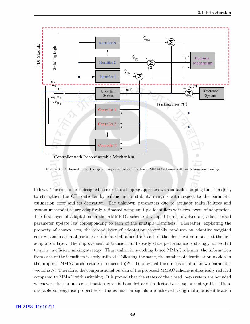
3.1 Introduction
Identifier N
Identifier 1
Identifier 2
SystemUncertain
Decision
Mechanism
Reference
System
Controller 1
Controller 2
Controller N
+
+
+
-
-
-
+
-
u
u
u
N
2
1
x
x
x
(N)
(2)
(1)
x(t)xr(t)
e(t)Tracking error
Sw
itch
ing L
ogic
FD
I M
od
ule
Controller with Reconfigurable Mechanism
Figure 3.1: Schematic block diagram representation of a basic MMAC scheme with switching and tuning
follows. The controller is designed using a backstepping approach with suitable damping functions [69],
to strengthen the CE controller by enhancing its stability margins with respect to the parameter
estimation error and its derivative. The unknown parameters due to actuator faults/failures and
system uncertainties are adaptively estimated using multiple identifiers with two layers of adaptation.
The first layer of adaptation in the AMMFTC scheme developed herein involves a gradient based
parameter update law corresponding to each of the multiple identifiers. Thereafter, exploiting the
property of convex sets, the second layer of adaptation essentially produces an adaptive weighted
convex combination of parameter estimates obtained from each of the identification models at the first
adaptation layer. The improvement of transient and steady state performance is strongly accredited
to such an efficient mixing strategy. Thus, unlike in switching based MMAC schemes, the information
from each of the identifiers is aptly utilized. Following the same, the number of identification models in
the proposed MMAC architecture is reduced to(N +1), provided the dimension of unknown parameter
vector is N . Therefore, the computational burden of the proposed MMAC scheme is drastically reduced
compared to MMAC with switching. It is proved that the states of the closed loop system are bounded
whenever, the parameter estimation error is bounded and its derivative is square integrable. These
desirable convergence properties of the estimation signals are achieved using multiple identification
49
TH-2198_11610211

3. Adaptive Multiple Model Fault Tolerant Control (AMMFTC) of Nonlinear UncertainSystems with Actuator Failures
Figure 3.2: Bidirectional robustness interactions transformed to unidirectional interaction under the proposed FTCstrategy
models with two layers of adaptation independent of the boundedness of the regressor matrix. It is
therefore concluded that the proposed FE/FTC strategy transforms the bidirectional interaction to a
unidirectional one as shown in Figure 3.2 (right). Hence, the design modularity is restored and the BIBS
design presumption on the system dynamics is eliminated. Furthermore, finite and infinite actuator
failures apart from unknown parametric uncertainties are also observed to be compensated using a
single controller without switching between identifiers or controllers. Thus, a piecewise continuous and
smooth control signal is obtained and the assumption of existence of positive dwell time is relaxed.
Hence, relative to existing results in literature with relevance to the problem of compensating finite
and infinite actuator failures, the major contributions of this chapter are enumerated below.
• To the best of the authors’ knowledge, this is the first time that an MMAC strategy is proposed to
compensate possibly infinite actuator failures. The proposed control scheme ensures boundedness
of closed loop signals. The incorporation of a two layer adaptation without switching into the
control design results in substantial improvement in transient and steady state performance,
under no failure, finite and infinite actuator failure scenarios with almost no additional control
usage. The proposed MMAC strategy from its design perspective overcomes all the limitations of
earlier multiple model adaptive controllers and hence can be applied to a wider class of nonlinear
uncertain systems. Thus, the work presented in this chapter contributes to bridge the potential
research gaps in MMAC as well as active FTC literature for nonlinear dynamical systems.
• A rigorous integrated stability analysis of the closed loop system under infinite actuator failures
for all t ∈ [0,∞) is conducted using a piecewise defined Lyapunov function. A piece of time herein
defines the time interval within which the actuator failure pattern does not change. Since occur-
rence of infinite actuator failures is not deterministic, the closed loop system is first represented
as a random nonlinear impulsive system in terms of the piecewise Lyapunov function (PLF).
Thereafter, a subsequent recursive formulation of the closed-loop system dynamics in terms of
the PLF is arrived at. Global boundedness of closed loop trajectories over all time t ∈ [0,∞),
is concluded thereafter. Unlike [6, 75], explicit expressions for L∞ and L2 bounds on the output
tracking error are derived for t ∈ [0,∞) considering both first and second layer of adaptation.
• The interrelation of the output transient performance bounds with the minimum transit time
50
TH-2198_11610211

3.2 Adaptive Multiple Model Fault Tolerant Control (AMMFTC) for Infinite Actuator Failures
between two consecutive changes in failure patterns and controller gains is mathematically de-
duced.
• In case of finite actuator failures or no failure conditions, global asymptotic (exponential) stability
of output tracking error is established. Further, the transient performance improvement using
the proposed MMAC strategy over single model adaptive control is theoretically proved.
• Decoupling between the controller and the identifier in the proposed MMAC based FE/FTC
scheme provides greater design freedom in determining the type of parameter estimator.
• The proposed MMAC scheme with two layer adaptation is further applied to FTC design prob-
lem for uncertain nonlinear coupled MIMO systems affected by finite actuator failures. Similar
stability properties and convergence characteristics are obtained. Further, transient and steady
state performance improvements are observed at the output without any significant increment
in the control usage. Results obtained through extensive simulation studies support theoretical
propositions. Further, experimental validation on a twin rotor MIMO system demonstrates the
practical feasibility and applicability of the proposed MMAC technique.
In view of the above design attributes and advantages, the proposed AMMFTC algorithm proves to
be an appealing choice for applications demanding reinforced robust stability and high performance.
The chapter is organized as follows: Section 3.2 discusses the proposed adaptive FTC design for
multi input single output (MISO) nonlinear systems affected by infinite actuator failures. The design
methodology spans through subsections 3.2.1-3.2.2 followed by closed-loop stability analysis in subsec-
tion 3.2.3.1 and transient performance analysis in subsection 3.2.3.2. An extensive simulation study is
provided in subsection 3.2.4. Next, the proposed MMAC approach is extended for application to the
problem of FTC design in MIMO nonlinear systems in Section 3.3. The problem formulation, control
design methodology, stability analysis and simulation study are provided in subsections 3.3.1-3.3.4.
Experimental study on a twin rotor MIMO system using the proposed AMMFTC is provided under
subsection 3.3.5. followed by summary in Section 3.4.
3.2 Adaptive Multiple Model Fault Tolerant Control (AMMFTC) for
Infinite Actuator Failures
In this section, an adaptive control strategy will be developed for nonlinear systems with parametric
uncertainties and affected by possibly infinite actuator failures.
51
TH-2198_11610211

3. Adaptive Multiple Model Fault Tolerant Control (AMMFTC) of Nonlinear UncertainSystems with Actuator Failures
3.2.1 Problem Statement
The same class of multi-input-single-output (MISO) nonlinear uncertain systems is considered as
in [6] and is rewritten below for completeness,
xi = xi+1 + fi(xi)Tκ∗, i = 1, ℘− 1
x℘ = f0(x, η) + f℘(x, η)T κ∗ +
m∑
j=1
bjβj(x, η)uj
η = Λ0(x, η) +
p∑
i=1
κ∗iΛi(x, η)
y = x1 (3.1)
where,the state vector is defined as x := [x1, x2, . . . , x℘]T ∈ R
℘ and xi := [x1, x2, . . . , xi]T ∈ R
i.
The term ℘ is the relative degree of the system concerned with x1 as the output. The nonlinearities
fi(x, η) : R℘ × R
n−℘ → Rp for i = 0, ℘ are assumed to be vectors of known smooth functions. The
actuation functions βj(x, η) : R℘ × R
n−℘ → R ∈ C∞ for j = 1,m are known and may be linear or
nonlinear in its arguments. The function y(t) ∈ R defines the system output and uj : [0,∞) → R
represents the jth control input or rather the output from the jth actuator fed to the plant. Further,
κ∗ := [κ∗1, κ∗2, . . . , κ
∗p]T ∈ R
p and bjmj=1 defines the vector of unknown parameters of the plant and
unknown actuation coefficients, respectively.
Now, in general, the output of the jth actuator given by uj is equal to its input uHj. However, the
actuators in the system may experience malfunctioning in the form of partial loss of effectiveness
(PLOE), lock-in-place (LIP) and float failures. Further, the actuator failures can occur intermittently
and hence, the cardinality of such events are not limited to (m − 1). Nevertheless, one actuator
should always remain healthy at any failure instant to satisfy the controllability criterion. Therefore,
a unified model reflecting the input-output (i/o) characteristics of the jth actuator encompassing the
aforementioned types of faults/failures for, t ∈ [toj,h, tej,h), h ∈ Z+ is given below [6].
uj(t) =
Kj,huHj + uFj,h, t ∈ [toj,h, t
ej,h)
uHj, t ∈ [tej,h, toj,h+1)
(3.2)
Herein, h = 1, 2, . . . ,∞ and Kj,h ∈ [0, 1] define the cardinality of occurrence of actuator failures and
the state of health of the jth actuator at the hth instant of the failure. The term uHj is the designed
control input to be fed to the jth actuator and uj defines the jth input of the system. The time
variables toj,h and tej,h denote the time instances at which the hth failure of the jth actuator commences
and ends, respectively. Further, the jth actuator remains healthy for the time interval [tej,h, toj,h+1) until
the onset of the (h + 1)th failure at t = toj,h+1. In addition, during the time [toj,h, tej,h), the degree of
severity of the jth actuator failure described by Kj and the value at which the actuator is stuck under
LIP failure are unknown.
The actuator failure model in (3.2) encompasses i/o characteristics of healthy actuators as well as
typical PLOE, LIP and float actuator failures.
52
TH-2198_11610211

3.2 Adaptive Multiple Model Fault Tolerant Control (AMMFTC) for Infinite Actuator Failures
• Kj,h = 1 and uFj,h = 0 for j = 1,m, means that the actuators are free from faults and failures.
• Kj,h ∈ (0, 1) and uFj,h = 0 for j = 1,m in (3.2) indicates that the actuator suffers from partial
loss of effectiveness (PLOE).
• Kj,h = 0 and uFj,h 6= 0 for j = 1, q with q ≤ m − 1 in the fault model (3.2) reveals that the
actuator undergoes a total loss and such a failure typically leaves the actuator jammed at an
unknown value denoted by uFj,h. Further, Kj = 0 and uFj,h = 0 for j = 1, q with q ≤ m − 1
describes actuator float failures.
Prior to the problem statement, the following assumptions are necessary.
Assumption 3.1. The nonlinear dynamical system in (3.1) is so designed that the desired output
performance can only be achieved in the event of at most q ≤ m−1 actuator failures unknown in time,
pattern and magnitude.
Assumption 3.2. The actuators are assumed to undergo a transition from their normal mode of
operation to various failure modes and vice-versa, infinitely many times. Therefore, there exists a
non-zero finite transit time T ∗ := toj,h+1 − tej,h > 0 between the occurrence of two consecutive actuator
failure patterns. (This assumption is justified later to be instrumental to achieve global boundedness of
all closed loop signals)
Assumption 3.3. The actuation functions in (3.1), given by βj(x, η) are assumed to be non-zero and
the sign of the actuation coefficients, that is, sign(bj) for j = 1,m are known.
Assumption 3.4. The reference trajectory and its successive time derivative signals (yr, yr, yr, . . . , y(℘)r )
are known, piecewise continuous, bounded and hence belong to a compact set.
Assumption 3.5. The upper/lower bounds on actuation coefficients 0 < bj ≤ |bj | ≤ bj, |uFj,h| < u
and 0 < Kj ≤ Kj ≤ 1 are known which means that bj , bj, umax and Kj for j = 1,m are known
finite positive constants. The unknown parameter vector κ∗ belongs to a known convex compact set,
i.e., κ∗ ∈ Sκ∗ ⊂ Rp. Here, Sκ∗ denotes the parameter space in R
p and ∀κ1, κ2 ∈ Sκ∗, the relation
‖κ1 − κ2‖ ≤ κmax holds.
Assumption 3.6. The subsystem dynamics given by η = Λ0(x, η) +p∑i=1
κ∗iΛi(x, η) is input-to-state-
stable (ISS) with x as its input. This implies that system dynamics is assumed to exhibit a minimum
phase behavior.
Having stated the assumptions, the control objectives of this work are as follows:
• To compensate the adverse effects of infinite actuator failures unknown in time, pattern and
magnitude and ensure boundedness of all closed loop signals ∀t ∈ [0,∞) in presence of unknown
parametric uncertainties.
• To enhance the output transient performance at start-up and in the event of unknown actuator
failures considered in (3.2). The aim is to quantify the output transient performance using L2
53
TH-2198_11610211
3. Adaptive Multiple Model Fault Tolerant Control (AMMFTC) of Nonlinear UncertainSystems with Actuator Failures
and L∞ bounds and thereafter prove the improvement in transient performance theoretically. It
is worth mentioning that usually, an improved output performance is achieved at the cost of high
input usage. However, such a practice may result in a degraded input performance. Thus, the
control design algorithm is to be aimed at guaranteeing a promising output transient performance
without any significant increment of the control energy spent. The intended objective behind is
to surpass the conventional trade-off between output and input performance at both instances of
start-up and post actuator failures.
• To ensure that the output tracking error y−yr converges to a arbitrarily small set in the vicinity
of the origin. Further, explicit expressions to calculate the ultimate bounds on the tracking error
are to be derived.
• To achieve asymptotic stability of the tracking error dynamics in the event of finite actuator
failures, i.e., limt→∞
(y(t) − yr(t)) = 0.
3.2.2 Adaptive Fault Tolerant Control Design
Firstly, for simplicity of representation, let us define the index set of actuators as B := j1, j2, . . . , jm.Thereafter, another two subsets of B as BtotF := j1, j2, . . . , jqh and BtotH := B/BtotF are defined.
Denoting Th for h ∈ Z+ to be the time instant when the failure pattern changes, it has been discussed
in the previous section that the fault pattern remains fixed until the time instant Th+1. Further, in
accordance with Assumption 3.4, stable solutions to the adaptive fault tolerant control problem can
be ensured only if there are at most qh(0 ≤ qh ≤ m − 1) actuator failures during the time interval
(Th, Th+1). Therefore, the set BtotF contains indices corresponding to totally failed actuators. How-
ever, the remaining healthy and partially failed actuator indices belong to the set BtotH . Incorporating
the actuator failure model (3.2) into the system dynamics and substituting the jth control input as
uHj = sign(bj)v/βj unfolds two different dynamical equations at the ℘th step corresponding to faulty
and fault free conditions as shown below.
• No fault condition
x℘ = f0(x, η) + f℘(x, η)Tκ∗ +
m∑
j=1
|bj|v (3.3)
• Faulty condition
x℘ = f0(x, η) + f℘(x, η)T κ∗ +
∑
j∈BtotH
Kj,h|bj|v +∑
BtotF
bjuFj,hβj (3.4)
Therefore, a unified mathematical model with an actuator failure parametrization encompassing faulty
and fault-free system dynamics in (3.4) and (3.3) can be framed as,
xi = xi+1 + fi(xi)Tκ∗, i = 1, ℘− 1
x℘ = f0(x, η) + f℘(x, η)T κ∗ + b∗v + βT u∗ (3.5)
54
TH-2198_11610211

3.2 Adaptive Multiple Model Fault Tolerant Control (AMMFTC) for Infinite Actuator Failures
where,
b∗ :=
m∑j=1
|bj|, for Kj,h = 1 and uFj,h = 0∀ j ∈ B
∑j∈BtotH
Kj,h|bj |, for Kj,h ∈ [0, 1) and uFj,h 6= 0 ∀ j ∈ BtotF
(3.6)
u∗ := [0, . . . , 0]T ∈ Rm, for Kj,h = 1 and uFj,h = 0 ∀ j ∈ B (3.7)
u∗ := [bjk uFjk,hqhk=1, 0, . . . , 0]
T ∈ Rm for Kj,h ∈ [0, 1) and uFj,h 6= 0 ∀ j ∈ BtotF (3.8)
Further, β := [βj(x, η)mj=1]T ∈ R
m is the vector of actuation functions. The unknown system
parameters and those induced due to actuator failures are redefined using a lumped parameter vector
θ∗ := [θ∗1, θ∗2, θ
∗3]T = [b∗, κ∗, u∗]T ∈ R
m+p+1. The actuator failure induced unknown parameters
θ∗1 and θ∗3 are time varying and hence are characterized by piecewise constant time dependent signals
instead of being constants for all t > 0. These parameters experience jumps at the occurrence of abrupt
actuator faults and failures. Therefore, from assumption 3.5, it is further assumed that θ∗1 ≥ ℓ :=
min1≤j≤mKjbj > 0. Besides, at the time instant t in the event of occurrence of an actuator failure,
the failure induced parameter jumps satisfy |θ∗1(t+)−θ∗1(t−)| ≤m∑j=1
bj−ℓ and |θ∗3j(t+)−θ∗3j(t−)| ≤ 2bju.
Since, one actuator should always be alive to satisfy the controllability condition, the inequality b∗ > ℓ
holds. Given that the parametrization of the fault affected system is complete (referred to (3.5)), it
is now possible to proceed with the design of the proposed multiple model estimator based indirect
adaptive backstepping controller to compensate possibly infinite actuator failures.
3.2.2.1 Parameter Estimation using Multiple Identifiers with Dual Layer Adaptation
In this section, firstly the design of the online parameter estimator using multiple identification
models with first layer of adaptation is explained. Thereafter, a piecewise stability analysis is conducted
to infer the boundedness and convergence properties of parameter estimation error and observer error
dynamics corresponding to each of the multiple (N) adaptive identification models.
To initiate the design of observers, the fault/failure parameterized dynamics in (3.5) are rewritten
in parametric x-model as,
x = f(x) + ΦT (x, v)θ∗ (3.9)
Wherein the function vector f(x) and the regressor matrix Φ(x, v) are defined as,
f(x) = [x2, x3, . . . , x℘, f0(x, η)]T ∈ R
℘ & ΦT (x, η) =
0 f1(x1)T 01×m
0 f2(x2)T 01×m
......
...
v fp(x, η)T βT
∈ R
℘×p+m+1. (3.10)
From assumption 3.9, it is known that the unknown parameter vector resided within a closed compact
55
TH-2198_11610211

3. Adaptive Multiple Model Fault Tolerant Control (AMMFTC) of Nonlinear UncertainSystems with Actuator Failures
set Sθ∗ defined as
Sθ∗ := [θ∗1, θ∗1] × [θ∗21, θ
∗21] × . . .× [θ∗2p, θ
∗2p] × [θ∗31, θ
∗31] × . . .× [θ∗3m, θ
∗3m]
Where, θ∗i and θ∗i denote the lower and upper bounds on the unknown parameters θ∗i for i = 1, . . . , (p+
m+ 1).
A. First Layer Adaptation
The N adaptive identifiers/estimators are described by differential equations with non-zero initial
values of the unknown parameter vector as follows,
˙x(µ) = Aµ(x, t)(x(µ) − x) + f(x) + ΦT (x, v)θ(µ) (3.11)
θ(µ)(t) = θ(µ)(t0) + Γµ
∫ t
t0
Proj[Φ(x, v)Pµ(x− x(µ))]dτ (3.12)
The subscript µ = 1, . . . , N denotes each of the adaptive identification models, x(µ) and θ(µ) are
the estimates of the state vector and the unknown parameter vector θ∗, respectively from the µth
identification model. The operator Proj· is a smooth projection operator to ensure that the parameter
estimate θ(µ) resides in Sθ∗ . The matrix Aµ(x, t) := Aµ0 − γΦ(x, v)TΦ(x, v)Pµ is so chosen to ensure
boundedness of µth estimator error dynamics irrespective of the boundedness of the regressor matrix
Φ(x, v) for µ ∈ 1, 2, . . . , N. The adaptation rate for each of the N models is given by a user designed
positive definite matrix Γµ ∈ Rp+m+1×p+m+1. Further, Aµ0 is a stable matrix satisfying the Lyapunov
equation, that, is,
ATµ0Pµ + PµAµ0 = −Qµ, Pµ, Qµ ∈ R℘×℘ and µ = 1, . . . , N (3.13)
In addition Pµ and Qµ are positive definite symmetric matrices chosen by the designer and may have
the same values for all the N identification models.
Let us now define the identification error and the parameter estimation error corresponding to the
µth identification model as x(µ) := x − x(µ) and θ := θ∗ − θ(µ), respectively for µ ∈ 1, 2, . . . , N.Referring to equations (3.11)-(3.12), the identification error dynamics for each of the N adaptive
estimators are derived as,
˙x(µ) = (Aµ0 − γΦ(x, v)TΦ(x, v)Pµ)x(µ) + ΦT (x, v)θ(µ) (3.14)
where, θ(µ)(t0) ∈ Ω(t0) ⊆ Sθ∗ for µ = 1, 2, . . . , N . The stability and convergence properties of all the
N adaptive estimators are summarized in Theorem 3.1. Since the FTC design aims at compensating
infinite actuator failures, following a piecewise stability analysis at this point would be helpful in
analyzing the stability of the overall closed loop system dynamics for t ∈ [0,∞). It is assumed that
the actuator fault/failure pattern does not change within the time interval [Th, Th+1) for h ∈ Z+.
Remark 3.1. The rationale behind the use of N adaptive identification models is to improve the
output transient performance. Now, considering the parameter space Sθ∗ defined earlier, the number
of identification models required is given by N = 2p+m+1. Therefore, the nonzero initial values of the
56
TH-2198_11610211
3.2 Adaptive Multiple Model Fault Tolerant Control (AMMFTC) for Infinite Actuator Failures
unknown parameter estimates θ(µ) with respect to each of the N adaptive identifiers should be so chosen
such that Sθ∗ ⊇ Ω(t0). Ω(t0) is a convex set formed by the initial parameter estimates θ(µ)(t0)Nµ=1
and the actual unknown parameter vector θ∗ resides in the set Ω(t0). Nevertheless, it is evident that
as the number of unknown parameters increase, the number of identification models N also escalates.
Although increment in the number of models results in a fair transient performance, it is achieved at
the cost of a high computational complexity. Increase in computational burden manifests itself in the
form of input delays, state delays and communication delays in real time systems resulting in degraded
system behavior and is therefore not desirable in safety critical applications.
Theorem 3.1. (First layer of adaptation) Let us consider that the solutions of the adaptive identifiers
given by (3.11)-(3.12) and the identification error dynamics in (3.14) for µ = 1, . . . , N, are defined
on the interval [Th, Th+1). Then the following properties hold under the framework of first layer
adaptation for each of the N adaptive identification models for Γµ, Pµ, Qµ > 0.
(i) θ(µ)(t) ∈ L∞[Th, Th+1)
(ii) x(µ)(t) ∈ L2[Th, Th+1) ∩ L∞[Th, Th+1), ˙x(µ)(t) ∈ L∞[Th, Th+1)
(iii)˙θ(µ)(t) ∈ L2[Th, Th+1)
Proof.
Let us take a Lyapunov function V(µ),h(x(µ), θ(µ), t) : R℘ × R
p+m+1 × [Th, Th+1) as,
V(µ),h =1
2xT(µ)Pµx(µ) +
1
2θT(µ)Γ
−1µ θ(µ) (3.15)
Given the identification error dynamics (3.14) and owing to the fact that the failure pattern remains
fixed for [Th, Th+1) results in,˙θ = − ˙
θ for [Th, Th+1). The first time derivative of V(µ) yields the
following,
V(µ),h = −xT(µ)Qµx(µ) − γxT(µ)PµΦTΦPµx(µ) + θT(µ)ΦPµx(µ) − θT(µ)Γ
−1µ
˙θ(µ) (3.16)
where the matrix Qµ := −(ATµ0Pµ + PµAµ0)/2 > 0 and as defined earlier, Pµ is a positive definite
symmetric matrix. Substituting the parameter update law (3.12) in (3.16) and using the properties
of projection operator from [69] as −θT(µ)Γ−1µ Proj(ΓµΦPµx(µ)) ≤ −θT(µ)Γ
−1µ ΓµΦPµx(µ), we arrive at the
following,
V(µ),h ≤ −λ(Qµ)‖x(µ)‖2 − γ‖ΦPµx(µ)‖2 < 0 (3.17)
Thereafter, integrating the above inequality (3.17) for the time interval t ∈ [Th, Th+1), rearranging
and using the notation xTPx = ‖x‖2P yields,
‖x(µ)‖L2[Th,Th+1) =1
√2λ(Qµ)
(‖x(µ)(Th)‖2Pµ
+ ‖θ(µ)(Th)‖2Γ−1
µ)
12 (3.18)
57
TH-2198_11610211
3. Adaptive Multiple Model Fault Tolerant Control (AMMFTC) of Nonlinear UncertainSystems with Actuator Failures
Since a projection operator is used for parameter estimation, it is very straightforward to conclude
that θ(µ) ∈ L∞[Th, Th+1). Further, from (3.18) and the inequality xT(µ)Pµx(µ) ≤ 2V(µ)(t) ≤ 2V(µ)(Th),
the signal properties x(µ)(t) ∈ L2 ∩L∞ are inferred. From the above arguments, ˙x(µ)(t) ∈ L∞ follows.
Thereafter using (3.17), the L2-integrability is proved and its L2 bound is given as,
‖ ˙θ(µ)‖L2[Th,Th+1) =
√λ(Γ2
µ)
2γ(‖x(µ)(Th)‖2
Pµ+ ‖θ(µ)(Th)‖2
Γ−1µ
)12 (3.19)
The proof is complete.
Now, to develop the proposed parameter estimation procedure based on multiple models, the following
lemma would be helpful.
Lemma 3.1. Let us consider the N adaptive estimators defined by (3.11) and the adaptive laws given
in (3.12) with initial conditions θ(µ)(t0) ∈ Ω(t0). If the unknown parameter vector θ∗ is contained in
the convex hull Ω(t0) of the set θ(µ)(t0)Nµ=1, then it also resides within the convex hull Ω(t) of the set
θ(µ)(t)Nµ=1∀t ≥ t0.
Proof. The proof is simple and follows from the linear algebra of convex sets.
B. Second Layer of Adaptation
Speed and accuracy of unknown parameter estimation θ, are two essential attributes which primarily
decide the output performance of an indirect adaptive control system. Essentially, since the proposed
design assumes the knowledge of unknown parameter bounds, such bounds may be located far away
from the actual parameter vector θ∗. Hence, the lumped parameter space Sθ∗ can be arbitrarily
large and therefore the estimation from each of the N observers with first layer of adaptation will
experience a slow parameter estimation with high overshoots exhibiting oscillatory behavior. This
will eventually translate in a degradation of the output transient performance, which is undesirable in
safety critical applications. Consequently, exploiting the convex set properties of the parameter space
Sθ∗ in Lemma 3.1, a second layer of adaptation is resorted to in order to achieve a fast and accurate
estimation of unknown parameters. From the theory of convex sets and convex hull, it is clear that
the initial parameter estimation set Ω(t0) ⊂ Sθ∗ can still enclose the actual parameter vector θ∗ if the
number of adaptive identification models is chosen to be N = p+m+ 1 + 1. Following this procedure
can significantly decrease the number of estimation models thereby reducing computational burden.
In the second adaptation layer, a weighted convex combination of the parameter estimates θ(µ) for
µ = 1, . . . , N with adaptive learning is resorted to. The rationale behind such a combination is
that the estimate of the parameter vector after such a weighted combination gains closer proximity to
the actual parameter vector θ∗ in the convex set Sθ∗ compared to θ(µ) from each of the (p + m + 2)
identification models (indexed by µ = 1, . . . , p + m + 2) with every iteration and results in fast
estimation.
The procedure is mathematically described as follows. Let the weighted convex combination of the
parameter estimates obtained from first adaptation layer be denoted as θs. As per definition the final
58
TH-2198_11610211

3.2 Adaptive Multiple Model Fault Tolerant Control (AMMFTC) for Infinite Actuator Failures
parameter estimate is mathematically represented as,
θs :=
(p+m+2)∑
µ=1
w∗µθ(µ), w∗
µ ∈ [0, 1] and
(p+m+2)∑
µ=1
w∗µ = 1
where, w∗µ for µ = 1, . . . , p+m+ 2 are the weights assigned to the parameters estimated for the N
identification models. However, these weights would be generally unknown and time varying depending
on the uncertainties affecting the system. Therefore, a Lyapunov based adaptive weight learning law
is formulated which eliminates the requirement of the knowledge of weight parameters w∗µ. In what
follows next, the formulation of the weight update law is presented and its stability properties are
derived.
In order to formulate the update laws for adaptive weight learning, constructing a suitable estimation
model is necessary and is formed as follows. A similar approach as presented in [121], is adopted for
learning the weights wµ online. Assuming θ∗ =p+m+2∑µ=1
w∗µθ(µ), and subtracting θ∗ from both sides
yields,p+m+2∑µ=1
w∗µ(θ(µ) − θ∗) = 0. Taking the time derivative of the resulting equality leads to,
p+m+2∑
µ=1
w∗µ(
˙θ(µ) − θ∗) = 0 (3.20)
Rearranging the above equation (3.20) gives,
p+m+1∑
µ=1
w∗µ(
˙θ(µ) − ˙
θ(p+m+2)) = − ˙θ(p+m+2) =⇒
p+m+1∑
µ=1
w∗µ(x(µ) − x(p+m+2)) = −x(p+m+2) (3.21)
Defining w∗ := [w∗µp+m+1
µ=1 w∗p+m+2]
T , w∗ := [w∗µp+m+1µ=1 ]T , X(t) := [diagx(µ)−x(p+m+2)p+m+1
µ=1 ] ∈R℘×(p+m+1) and r(t) := −x(p+m+2) ∈ R
℘, equation (3.21) can be rewritten in a vector form as,
X(t)w∗ = r(t). Therefore, since the elements of the vector X(t) and r(t) are known with the
weight vector w∗ being unknown, the weight estimation model can be framed as,
X(t) ˆw = r(t) (3.22)
Further, using the weight estimation model (3.22), the weight update law is chosen as
˙w(t) = −X(t)TX(t) ˆw(t) + X(t)T r(t); wp+m+2 = 1 −p+m+1∑
µ=1
wµ (3.23)
Finally, the unknown parameter vector θ∗ is estimated as θs :=p+m+2∑µ=1
wµθ(µ).
Theorem 3.2. Let us consider the second layer of adaptive parameter estimate θs :=p+m+2∑µ=1
wµθ(µ)
59
TH-2198_11610211

3. Adaptive Multiple Model Fault Tolerant Control (AMMFTC) of Nonlinear UncertainSystems with Actuator Failures
and the weight learning law given by (3.23) defined within the time interval [Th, Th+1). The following
properties hold: (i) w ∈ L∞[Th, Th+1); (ii) ˙w ∈ L∞[Th, Th+1).
Proof.
To prove the properties of the adaptive weight estimates wµ for µ = 1, . . . , p +m + 2, a Lyapunov
function defined over the time interval [Th, Th+1) is called upon as Vw,h : Rp+m+1 × [Th, Th+1) → R+
given by,
Vw,h =1
2˜wT (t) ˜w(t) (3.24)
where, ˜w(t) := w∗(t)− ˆw(t). Taking the time derivative of Vw,h and the subsequent substitution of the
weight adaptation law (3.23) yields,
Vw,h = −(w∗ − ˆw)T (−X(t)TX(t) ˆw(t) + X(t)TX(t)w∗(t))
= −(w∗ − ˆw)TX(t)TX(t)(w∗ − ˆw) = − ˜w(t)TM(t) ˜w(t) < 0 (3.25)
Here, M(t) := X(t)TX(t) > 0 and since Vw,h is negative definite, integrating both sides of the
equality (3.25) in the interval [Th, Th+1) and using Hölder’s inequality results in,
−∫ Th+1
Th
Vw,h(t)dt ≤ ‖M‖∞∫ Th+1
Th
˜wT (t) ˜w(t)dt <∞ (3.26)
Therefore, the negative definiteness of Vw,h and the above inequality (3.26) proves that ˆw, w ∈L∞[Th, Th+1) and ˙w ∈ L∞[Th, Th+1). Further, wp+m+2 is also bounded. The proof is complete.
3.2.2.2 Backstepping Control Design
The design procedure is initiated by defining the error variables as,
z1 = x1 − yr, (3.27)
zi = xi − αi−1 − y(i−1)r (3.28)
where i = 2, ℘. Now utilizing the plant dynamics in (3.1), and taking the first time derivative of the
error variables yields,
zi = zi+1 + αi + fi(xi)θ∗2 − αi−1 (3.29)
z℘ = f0(x, η) + f℘(x, η)T θ∗2 + θ∗1v + βT θ∗3 − α℘−1 (3.30)
60
TH-2198_11610211

3.2 Adaptive Multiple Model Fault Tolerant Control (AMMFTC) for Infinite Actuator Failures
Here i = 1, ℘− 1. The variables αi are the virtual control inputs stabilizing each of the tracking error
subsystem dynamics in zi (3.29)-(3.30). These stabilizing functions αi are given by (3.31).
αi = −zi−1 − cizi − ci‖ψi‖2zi − gi
∥∥∥∂αi−1
∂θ2
∥∥∥2zi − ψTi θ2 +
i−1∑
k=1
(∂αi−1
∂xkxk+1 +
∂αi−1
∂y(k−1)r
y(k)r
)(3.31)
with i = 1, ℘− 1 and ψi := fi(xi) −i−1∑k=1
∂αi−1
∂xkfk(xk). Due to actuator failure induced uncertainties,
the ℘th design step is quite different from the procedure followed in the previous steps. In Step ℘, the
controller design is initiated by defining the z℘-dynamics in an expanded form with the actual control
law v = v1 + v2, as follows.
z℘ = f0(x, η) + f℘(x, η)T θ2 + βT θ3 + θ1v1 + θ1v1 + θ∗1v2 − y(℘)
r −℘−1∑
k=1
(∂α℘−1
∂xkxk+1 −
∂α℘−1
∂y(k−1)r
y(k)r
)
+(βT θ3 + ψT℘ θ2 −
∂α℘−1
∂θ2
˙θ2
)(3.32)
The first part of the control input v(t) is chosen as follows,
v1 =1
θ1(−f0(x, η) − f℘(x, η)
T θ2 − βT θ3 − z℘−1 +
℘−1∑
k=1
(∂α℘−1
∂xkxk+1 −
∂α℘−1
∂y(k−1)r
y(k)r
)+ y(℘)
r ), (3.33)
Such a choice of v1(t) yields the resulting z℘-dynamics as given below,
z℘ = −z℘−1 + θ∗1v2 + θ1v1 + βT θ3 + ψT θ2 −∂α℘−1
∂θ2
˙θ2 (3.34)
Now being left with the design of v2 to arrive at the final control law v, the signal v2 is chosen as
follows,
v2 = ℓ−1(− c℘z℘ − c℘
(|v1|2 + ‖β‖2 + ‖ψ℘‖2
)z℘ − g℘
∥∥∥∂α℘−1
∂θ2
∥∥∥2z℘)
(3.35)
Thereafter, substituting the expression for v2 in (3.34) and using the sum of squares inequality leads
to,
z℘z℘ ≤ θ∗1ℓc℘z
2℘ +
1
4c℘
(‖θ1‖2 + ‖θ2‖2 + ‖θ3‖2
)+
‖ ˙θ2‖2
4g℘− z℘z℘−1 (3.36)
The inequality in (3.36) would be useful while deriving the stability results of the proposed control.
Finally, we arrive at the actual control law v(t) as,
v(t) = v1(t) + v2(t) (3.37)
61
TH-2198_11610211

3. Adaptive Multiple Model Fault Tolerant Control (AMMFTC) of Nonlinear UncertainSystems with Actuator Failures
Figure 3.3: Block diagrammatic representation of the proposed adaptive fault tolerant control scheme (AMMFTC).
where the signals v1(t) and v2(t) have been defined in the preceding text in equations (3.33) and (3.35).
The equations (3.29)-(3.30), (3.31) and (3.33)-(3.35) are the fundamental equations which would be
required in implementation of the proposed control law. The control design parameters ci, ci, g℘ are
positive scalars.
Figure 3.3 shows a schematic block diagram summarizing the proposed control design procedure.
3.2.3 Main Results
3.2.3.1 Stability Analysis of the Proposed Control System
Herein, prior to the closed loop stability analysis of the proposed adaptive control system, the fol-
lowing preliminary calculations and statements are necessary in the subsequent analysis. As mentioned
earlier, the compact set wherein the parameter θ∗ resides is denoted by Sθ∗ defined as,
Sθ∗ : = θ∗ ∈ Rp+m+1| ℓ ≤ θ∗1 ≤
m∑
j=1
bj , θ2 ∈ Sκ∗ ⊆ Rp, |θ∗3j | ≤ bj uj , j = 1,m (3.38)
Lemma 3.2. The projection operator utilized in the parameter estimation law (3.12) has the following
properties [69]: (i) The mapping Proj:Rp+m+1×Sθ∗ → Rp+m+1 is locally Lipschitz in its arguments; (ii)
ProjτTΓ−1µ Projτ ≤ τTΓ−1
µ τ ∀ θ(µ) ∈ Sθ∗; (iii) The solution θ(µ) remains in Sθ∗ ∀ θ(µ)(t0) ∈ Sθ∗;(iv) −θT(µ)Γ
−1µ Projτ ≤ −θT(µ)Γ
−1µ τ, ∀ θ(µ), θ
∗ ∈ Sθ∗.
Proof. The proof can be referred to [69] (Refer Lemma E.1 on page 512).
62
TH-2198_11610211
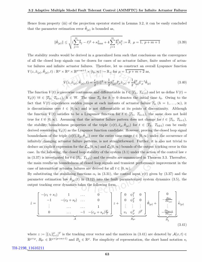
3.2 Adaptive Multiple Model Fault Tolerant Control (AMMFTC) for Infinite Actuator Failures
Hence from property (iii) of the projection operator stated in Lemma 3.2, it can be easily concluded
that the parameter estimation error θ(µ) is bounded as,
‖θ(µ)‖ ≤
√√√√(
m∑
j=1
bj − ℓ)2 + κ2max + 4
m∑
j=1
b2j u
2j := θ, µ = 1, p+m+ 1 (3.39)
The stability results would be derived in a generalized form such that conclusions on the convergence
of all the closed loop signals can be drawn for cases of no actuator failure, finite number of actua-
tor failures and infinite actuator failures. Therefore, let us construct an overall Lyapunov function
V (z, x(µ), θ(µ), t) : R℘ × R
℘ × Rp+m+1 × [t0,∞) → R+ for µ = 1, p +m+ 2 as,
V (z, x(µ), θ(µ), t) =ǫ
2‖z‖2 +
1
2xT(µ)Pµx(µ) +
1
2θT(µ)Γ
−1µ θ(µ) (3.40)
The function V (t) is piecewise continuous and differentiable in t ∈ [Th, Th+1) and let us define V (t) =
Vh(t) ∀t ∈ [Th, Th+1), h ∈ W. The time Th for h = 0 denotes the initial time t0. Owing to the
fact that V (t) experiences sudden jumps at each instants of actuator failure Th (h = 1, . . . ,∞), it
is discontinuous over t ∈ [0,∞) and is not differentiable at its points of discontinuity. Although
the function V (t) satisfies to be a Lyapunov function for t ∈ [Th, Th+1), the same does not hold
true for t ∈ [0,∞). Assuming that the actuator failure pattern does not change for t ∈ [Th, Th+1),
the stability/boundedness properties of the triple (z(t), xµ, θ(µ)) for t ∈ [Th, Th+1) can be easily
derived considering Vh(t) as the Lyapunov function candidate. However, proving the closed loop signal
boundedness of the triple (z(t), xµ, θ(µ)) over the entire time range t ∈ [0,∞) under the occurrence of
infinitely changing actuator failure patterns, is not straightforward. Further, it is also not trivial to
deduce an explicit expression for the L∞[0,∞) and L2[0,∞) bounds of the output tracking error in this
case. In the following, the closed loop stability of the system (3.1) under the action of the control law v
in (3.37) is investigated for t ∈ [Th, Th+1) and the results are summarized in Theorem 3.3. Thereafter,
the main results on boundedness of closed loop signals and transient performance improvement in the
case of intermittent actuator failures are derived for all t ∈ [0,∞).
By substituting the stabilizing functions αi in (3.31), the control input v(t) given by (3.37) and the
parameter estimation law˙θ(µ)(t) in (3.12) into the fault parameterized system dynamics (3.5), the
output tracking error dynamics takes the following form,
z =
−(c1 + s1) 1 . . . 0
−1 −(c2 + s2) . . . 0... . . . . . . 1
0 . . . −1 −(c℘ + s℘)b∗
ℓ
︸ ︷︷ ︸A
z +
0 ψT1 0
0 ψT2 0...
......
v1 ψT℘ βT
︸ ︷︷ ︸Bθ∗
θ(µ) +
0
− ∂α1∂κ(µ)
...
−∂α℘−1
∂κ(µ)
︸ ︷︷ ︸B ˙κ
˙κ(µ)
(3.41)
where z := [zi℘i=1]T is the tracking error vector and the matrices in (3.41) are denoted by A(x, t) ∈
R℘×℘, Bθ∗ ∈ R
℘×(p+m+1) and B ˙κ ∈ R℘. For simplicity of representation, the short hand notation si
63
TH-2198_11610211

3. Adaptive Multiple Model Fault Tolerant Control (AMMFTC) of Nonlinear UncertainSystems with Actuator Failures
in the matrix A, is used for the following expressions given below.
s1 = c1‖ψ1‖2, si = c2‖ψi‖2 + gi
∥∥∥∂αi−1
∂κ
∥∥∥2
(3.42)
s℘ = c℘(‖ψ℘‖2 + |v1|2 + ‖β‖2) + g℘
∥∥∥∂α℘−1
∂κ
∥∥∥2
(3.43)
As defined earlier, the parameters ci, ci and gj for i = 1, ℘ and j = 2, ℘ are positive design constants
chosen by the designer. Now, we are well equipped to state the following theorem.
Theorem 3.3. (Piecewise stability properties under first layer of adaptation) Let us consider the
output tracking error dynamics in (3.41) whose solutions are defined for t ∈ [Th, Th+1) for h ∈ W.
Under Assumptions 3.1-3.6, and the adaptive law˙θ(µ)(t) in (3.12), the solutions satisfy the following
properties: (i) z(t) ∈ L∞[Th, Th+1), x(t), z(t) ∈ L∞[Th, Th+1); (ii) z(t) ∈ L2[Th, Th+1). Further, if
Th+1 → ∞ and the actuator failure pattern remains fixed within [Th, ∞], asymptotic output tracking
is guaranteed, that is, limt→∞
z(t) = 0.
Proof of (i). The proof will be completed in two steps. In the first step, the boundedness of all the
closed loop signals shall be proved for the interval [Th, Th+1). Secondly, to prove asymptotic stability
of the tracking error z(t), it would be shown to belong to class of L2[Th, Th+1) integrable signals. A
Lyapunov function V (t) for t ∈ [Th, Th+1) defined as Vh(t) in (3.40) is therefore called upon. The
analysis is done as follows. Using (3.29),(3.30), (3.36) and invoking the sum of squares inequality with
θ∗ := [θ∗1 θ∗2 θ
∗3]T =: [b∗ κ∗ u]T yields,
d
dt
( ǫ2‖z‖2
)≤ −λ(Q)ǫ‖z‖2 +
ǫ
4
[‖θ1(µ)‖2
c℘+
‖θ2(µ)‖2
c+
‖θ3(µ)‖2
c℘+
‖ ˙κ‖2
g
]
≤ −λ(Q)ǫ‖z‖2 +ǫ
4
[‖b‖2
c℘+
‖κ‖2
c+
‖˜u‖2
c℘+
‖ ˙κ‖2
g
]
≤ −λ(Q)ǫ‖z‖2 +ǫ
4
[‖θ(µ)‖2
¯c+
‖ ˙θ(µ)‖2
g
](3.44)
where Q := diagc1, . . . , c℘−1,θ∗1ℓ c℘ > 0, c :=
℘∑i=1
14ci
, ¯c := minc, c℘, c℘ and g :=℘∑i=2
14gi
. From
Theorem 3.1, it is already proved that the projection operation within the set Sθ∗ ensures θi(µ) ∈L∞[Th, Th+1), i = 1, 3 and
˙θ(µ) ∈ L2[Th, Th+1) implying ‖ ˙κ‖ ∈ L2[Th, Th+1). Therefore, the differ-
ential inequality (3.44) is solved in the interval [Th, Th+1) for h ∈ W as,
‖z‖[Th, Th+1) ≤ ‖z(Th)‖e−λ(Q)t +1
2√λ(Q)
[‖θ(µ)‖2
∞¯c
+‖ ˙θ(µ)‖2
2
g
] 12
(3.45)
From (3.45), the property of z(t) ∈ L∞[Th, Th+1) is proved and since the reference trajectory and its
successive time derivatives are assumed to belong to a compact set so the plant state vector x(t) ∈L∞[Th, Th+1) and z ∈ L∞[Th, Th+1). Hence, the closed loop signal boundedness for t ∈ [Th, Th+1) (h ∈W) using the proposed controller is proved.
64
TH-2198_11610211

3.2 Adaptive Multiple Model Fault Tolerant Control (AMMFTC) for Infinite Actuator Failures
Proof of (ii).
Now it has to be shown that z(t) ∈ L2[Th, Th+1). Therefore, proceeding with the proof, let us first
represent the closed loop system in (3.41) using the definition θ∗1 = θ1 + θ1 as
z =
−(c1 + s1) 1 . . . 0
−1 −(c2 + s2) . . . 0... . . . . . . 1
0 . . . −1 −(c℘ + s℘)bℓ
︸ ︷︷ ︸A
z +
0 ψT1 0
0 ψT2 0...
......
v ψT℘ βT
︸ ︷︷ ︸Bθ∗
θ(µ) +
0
− ∂α1∂κ(µ)
...
−∂α℘−1
∂κ(µ)
︸ ︷︷ ︸B ˙κ
˙κ(µ)
Thereafter, the matrix Bθ∗ is factorized such that Bθ∗ := M(z, θ, t)ΦT (x, v). Where,
M(z, θ(µ), t) :=
1 0 . . . 0 0
−∂α1∂x1
1 . . . 0 0...
. . .. . .
. . ....
−∂α−1
∂x1−∂α−1
∂x2. . . −∂α−1
∂x−11
(3.46)
Hereafter, we define an auxiliary variable ϑ := z − Mx(µ). With this choice of ϑ, we arrive at a
dynamics in ϑ driven by only L2-integrable inputs x(µ) and ˙κ(µ) described by the following differential
equation defined for t ∈ [Th, Th+1).
ϑ = Aϑ+ [−M + AM−MAµ]︸ ︷︷ ︸M(z,θ(µ),t)
x(µ) +B ˙κ˙κ(µ) (3.47)
Now, finally if ϑ is shown to be L2-integrable in the interval [Th, Th+1), the tracking error z(t) ∈L2[Th, Th+1) is proved. Proceeding with this objective, we compute,
d
dt
(1
2‖ϑ‖2
)≤ ϑT Aϑ+ ϑTM(z, θ(µ), t)x(µ) + ϑTB ˙κ
˙κ(µ)
≤ −λ(Q)‖ϑ‖2 −℘∑
i=1
gi
∥∥∥∂αi−1
∂κ(µ)
∥∥∥2ϑ2i +
℘∑
i=1
∂αi−1
∂κ(µ)
˙κ(µ)ϑi + ϑTMx(µ)
d
dt
(1
2‖ϑ‖2
)≤ −λ(Q)‖ϑ‖2 +
‖ ˙κ(µ)‖2
4g+ ϑTMx(µ) (3.48)
Using Peter-Paul inequality (Appendix A.2.3) with the factor λ(Q) for the third term in (3.48) leads
to,
ϑTMx(µ) ≤ λ(Q)‖ϑ‖2
2+
1
2λ(Q)‖M‖2
F‖x(µ)‖2 (3.49)
Using (3.48) in (3.49) results in the following differential inequality given as,
d
dt
(1
2‖ϑ‖2
)≤ −λ(Q)‖ϑ‖2 +
‖ ˙κ(µ)‖2
4g+
‖M‖2F‖x(µ)‖2
2λ(Q)(3.50)
65
TH-2198_11610211

3. Adaptive Multiple Model Fault Tolerant Control (AMMFTC) of Nonlinear UncertainSystems with Actuator Failures
The boundedness of M(·) is ensured if M, M, A and A(µ) are bounded. The bounded variation of
M is inferred from the choice of the virtual control laws αi, i = 1, − 1 and control law v. Since
x ∈ L∞ as shown in the earlier section of the proof, the regressor Φ(x, v) and the matrix Aµ is
bounded. The matrix M is also found to be bounded in t taking into account the following signal
properties, z ∈ L∞[Th, Th+1),˙θ ∈ L2[Th, Th+1) and the partial derivatives ∂M
∂z ,∂M∂θ
being time
bounded continuous functions. Therefore, the matrix M(z, θ(µ), t) is bounded. Finally, the inequality
in (3.50) is rearranged and then integrated for the time interval [Th, Th+1) leading to,
∫ Th+1
Th
‖ϑ‖2dt ≤ ‖ϑ(Th)‖2
2λ(Q)+
1
4gλ(Q)
∫ Th+1
Th
‖ ˙κ(µ)‖2dt+1
2λ(Q)2‖M‖2
F
∫ Th+1
Th
‖x(µ)‖2dt <∞ (3.51)
With a reasonable consideration that ϑ(Th) is finite and ˙κ(µ), x(µ) ∈ L2[Th, Th+1), the signal property
of ϑ(t) ∈ L2[Th, Th+1) is easily concluded from (3.51). Further, z(t) ∈ L2[Th, Th+1) follows from
the L2-integrability property of ϑ(t). Finally, if Th+1 → ∞, invoking Barbalat’s Lemma [69], z(t) ∈L2[Th, ∞)∩L∞[Th, ∞) with z(t) ∈ L∞[Th, ∞) infers asymptotic stability of the tracking error vector
z(t). The proof is complete.
As mentioned earlier prior to Theorem 3.3, that the total Lyapunov function V (t) is discontinuous due
to sudden jumps at the actuator failure instances Th for h ∈ Z+. The initial time instant when no
fault occurs is indexed by h = 0 and given by T0. The magnitude of the jumps in V (t) at the failure
instants Th, can be calculated as,
V (T+h ) − V (T−
h ) ≤ 1
2θT(µ)(T
+h )Γ−1
µ θ(µ)(T+h ) − 1
2θT(µ)(T
−h )Γ−1
µ θ(µ)(T−h ) ≤ 1
2λ(Γ−1
µ )θ2
= ∆ (3.52)
Further, let us consider the entire time range, i.e, t ∈ [T0, T ), where T0 and T denote the initial and
final time instants. Within this time interval, assume that the actuator failure pattern changes ℵ times.
Therefore, using (3.52), the following inequality can be established.
V (T−) ≤ V (T+ℵ ) ≤ V (T−
ℵ ) + ∆ ≤ V (T−ℵ−1) + 2∆ ≤ . . .
≤ . . . ≤ V (T1) + (ℵ − 1)∆ ≤ V (T0) + ℵ∆ (3.53)
where ℵ denotes the total number of times the actuator failure pattern changes. From inequality (3.53),
it can be inferred that if the actuator failure patterns vary with finite cardinality (finite number of times)
for all t ∈ [T0, T ), the overall Lyapunov function V (T−) is bounded rendering global boundedness of
the closed loop signals. However, infinitely occurring actuator failures would mean that ℵ → ∞ with
T → ∞. Subsequent unboundedness of V (t) can be concluded from (3.53) for [T0, ∞) with infinite
actuator failures. Therefore, it is not straightforward to prove the stability of the closed loop adaptive
system affected by infinitely occurring actuator failures. In what follows, we provide a stability analysis
ensuring closed loop signal boundedness globally for all time t ∈ [T0, ∞) and ℵ → ∞. The theoretical
results obtained are stated in Theorem 3.4.
Theorem 3.4. (first layer of adaptation) Let us consider the closed loop adaptive system consisting of
the nonlinear system (3.1), the adaptive parameter estimation law (3.12) and the control law in (3.37).
66
TH-2198_11610211

3.2 Adaptive Multiple Model Fault Tolerant Control (AMMFTC) for Infinite Actuator Failures
By virtue of the assumptions 3.1-3.6 and choosing the initial time T0 = 0, the following results hold.
(i) All the closed loop signals are globally bounded assuming that the transit time T ∗ between actuator
failure pattern changes is finite. The tracking error z(t) finally resides within a bound is given
by,
limt→∞
‖z(t)‖ ≤
√√√√θ2
(ǫ+ 2λ(Γ−1
µ )¯c
ρ¯c
)(2 − e−ρT ∗
1 − e−ρT ∗
)+
2∆
1 − e−ρT ∗ (3.54)
(ii) The output tracking error z1 = x1 − yr is energy integrable for t ∈ [0, ∞) for a finite ℵ and the
L2[0, ∞) bound is given by,
‖z‖2 ≤
√√√√2‖z(0)‖2 + M∗‖x(µ)(0)‖2Pµ
+ (M∗ −M∗)(‖θ(µ)(0)‖2Γ−1
µ+ 2ℵ(0, ∞)∆)
2λ(Q)(3.55)
(iii) Asymptotic convergence of the output tracking error z(t) to the origin is ensured for a finite ℵ,
i.e., limt→∞
x1 − yr = 0.
Herein M∗ and M∗are user defined parameters. The parameters ¯c, γ, ρ := min2ρ, λ(Γ−1
µ ), ρ =
minλ(Q), λ(Qµ), ǫ := γλ(Γ−2µ )g and Γµ > 0 are design constant scalars and matrices. Further,
∆ is the maximum magnitude of the jump due to occurrence of actuator failure given in (3.52) and
ℵ(0, T ) denotes the total number of transitions the actuator failure pattern within the time interval
[0, T ). The notations λ(·) and λ(·) denote the minimum and maximum eigen values of the argument.
Proof of Theorem 3.4 (i)
To prove stability, the Lyapunov function candidate V (t) for t ∈ [Th, Th+1) defined as Vh(t) in (3.40)
is called upon. The analysis is done as follows. From the inequality (3.17) in the proof of Theorem 3.1
with the choice of Pµ = I℘, the following inequality is deduced.
d
dt
(1
2‖x(µ)‖2 +
1
2θT(µ)Γ
−1µ θ(µ)
)≤ −xT(µ)Qµx(µ) − γ‖ΦPµx(µ)‖2
≤ −λ(Qµ)‖x(µ)‖2 − γ
2λ(Γ−2
µ )‖ ˙θ(µ)‖2 (3.56)
Further, from (3.44), it has been found that the following inequality holds,
d
dt
( ǫ2‖z‖2
)≤ −λ(Q)ǫ‖z‖2 +
ǫ
4
[‖θ(µ)‖2
¯c+
‖ ˙θ(µ)‖2
g
](3.57)
Now as per the definition of Vh(t) in (3.40), and using the above inequalities (3.57) and (3.44), the
first time derivative of Vh(t) for t ∈ [Th, Th+1) is calculated as,
Vh(t) =d
dt
[ ǫ2‖z‖2 +
1
2‖x(µ)‖2 +
1
2θT(µ)Γ
−1µ θ(µ)
]
≤ −λ(Q)ǫ‖z‖2 − λ(Qµ)‖x(µ)‖2 −(γ
2λ(Γ−2
µ ) − ǫ
4g
)‖ ˙θ(µ)‖2 +
ǫ
4¯c‖θ(µ)‖2 (3.58)
67
TH-2198_11610211

3. Adaptive Multiple Model Fault Tolerant Control (AMMFTC) of Nonlinear UncertainSystems with Actuator Failures
Defining ρ := minλ(Q), λ(Qµ) and choosing ǫ = γλ(Γ−2µ )g and substituting these relations in (3.58)
yields the following with solutions being defined ∀t ∈ [Th, Th+1), h ∈ W,
Vh(t) ≤ −ρ(ǫ‖z‖2 + ‖x(µ)‖2) − 1
2θT(µ)Γ
−1µ θ(µ) +
[ǫ+ 2λ(Γ−1
µ )¯c
2¯c
]θ2
≤ −min2ρ, λ(Γ−1µ )
︸ ︷︷ ︸ρ
Vh(t) +
[ǫ+ 2λ(Γ−1
µ )¯c
2¯c
]θ2 ≤ −ρVh(t) +
[ǫ+ 2λ(Γ−1
µ )¯c
2¯c
]θ2
(3.59)
Now, stability of the overall control system affected by infinitely occurring actuator failures over the
time interval [0, ∞) cannot be inferred from the boundedness of Vh(t) or rather V (t) over the interval
[Th, Th+1). Therefore at this point, let us call upon the total Lyapunov function V (t) defined over
t ∈ [0, ∞). Due to the random variation in the actuator failure pattern at each unknown time
instant Th(h ∈ N), the Lyapunov function V (t) would undergo random jumps at the corresponding
time instances between intervals([Th, Th+1)) of continuous stable evolution in accordance with (3.59).
These instantaneous changes of V (t) can be approximately expressed as impulses. The overall system
under infinitely varying actuator failure patterns can now be represented as a type of hybrid system
comprising of continuous dynamics, discrete dynamics and the impulsive sequence Th ∀h ∈ W
satisfying 0 ≤ T0 < T1 < T2 < . . . < Th < . . . < Tℵ < T and T → ∞ as given below.
V (z, x(µ), θ(µ), t) ≤ −ρV (z, x(µ), θ(µ), t) +
[ǫ+ 2λ(Γ−1
µ )¯c
2¯c
]θ2, t ∈ [Th, Th+1) (3.60)
V (z, x(µ), θ(µ), Th+1) ≤ V (z, x(µ), θ(µ), T−h+1) + ∆, ∀h ∈ W (3.61)
Where, ∆ defined in (3.52) denotes the magnitude of jumps in the Lyapunov function V (t) at the failure
instances Th; V (T−h+1) := lim
t→T−
h+1
V (t) and θ denotes the upper bound on the parameter estimation error
defined earlier. Invoking the property of continuous dependence of solutions on initial conditions and
parameters stated in (Theorem 3.4, [109]), the solution of the differential inequality (3.61) for any time
interval [Th, Th+1) is given by,
V (t) ≤ V (Th)e−ρ(t−Th) +
t∫
Th
e−ρ(t−s)[ǫ+ 2λ(Γ−1
µ )¯c
2¯c
]θ2ds (3.62)
Let us assume that actuator failure pattern changes occur between the considered time range [0, T ) ⊃[Th, Th+1) with a finite cardinality ℵ(T0, T ) = (T − T0)/T
∗ and Tℵ < T < ∞. Now using (3.53) and
iterating the inequality (3.62), the following is obtained for t ∈ [T0, T ).
V (T−) ≤ V (T0)e−ρ(T−T0) +
[ǫ+ 2λ(Γ−1
µ )¯c
2¯c
]θ2
( T1∫
T0
e−ρ(T−s)ds+
T2∫
T1
e−ρ(T−s)ds+ . . .+
T∫
Tℵ(T0,T )
e−ρ(T−s)ds
)
+ ∆[e−ρ(T−T1) + e−ρ(T−T2) + . . .+ e−ρ(T−Tℵ(T0,T )−1) + e−ρ(T−Tℵ(T0,T ))
](3.63)
68
TH-2198_11610211

3.2 Adaptive Multiple Model Fault Tolerant Control (AMMFTC) for Infinite Actuator Failures
At this point, let us consider the initial time T0 = 0 and thereafter using the notation for the index of
the actuator failure pattern change h as defined earlier, the above inequality (3.63) is represented in a
more compact form as follows,
V (T−) ≤ V (0)e−ρT +
[ǫ+ 2λ(Γ−1
µ )¯c
2¯c
]θ2
ρ
( ℵ(0,T )−1∑
h=0
e−ρ(T−Th+1) −ℵ(0,T )−1∑
h=0
e−ρ(T−Th) − e−ρ(T−Tℵ(0,T )) + 1
)
+ ∆
[ ℵ(0,T )−1∑
h=1
e−ρ(T−Th) + e−ρ(T−Tℵ(0,T ))
](3.64)
It is known that two consecutive instances of occurrence of actuator failure are related by the transit
time T ∗ := Th+1 − Th. Further, considering the final time T with [Th, Th+1) ⊂ [0, T ] ∀h ∈ W, the
cardinality ℵ(0, T ) of the index set representing the number of changes in the actuator failure pattern
for t ∈ [0, T ) satisfies the inequality,
ℵ(T0, T ) = ℵ(0, T ) − h ≤ T − ThT ∗ , h ∈ 0, 1, 2, . . . ,ℵ(0, T ) ⊂ W (3.65)
The inequality above implies (T − Th+1) ≥ (ℵ(0, T )− h− 1)T ∗ and (T − Th) ≥ (ℵ(0, T )− h)T ∗ which
when substituted in (3.64) yields,
V (T−) ≤ V (0)e−ρT +θ2
ρ
[ǫ+ 2λ(Γ−1
µ )¯c
2¯c
][ ℵ(0,T )−1∑
h=0
e−ρ(ℵ(0,T )−h−1)T ∗
+ 1
]+ ∆
[ ℵ(0,T )−1∑
h=1
e−ρ(ℵ(0,T )−h)T ∗
+ 1
]
(3.66)
≤ V (0)e−ρT +θ2
ρ
[ǫ+ 2λ(Γ−1
µ )¯c
2¯c
](1
1 − e−ρT ∗ + 1
)+ ∆
(e−ρT
∗
1 − e−ρT ∗ + 1
)(3.67)
≤ V (0)e−ρT +θ2
ρ
[ǫ+ 2λ(Γ−1
µ )¯c
2¯c
](2 − e−ρT
∗
1 − e−ρT ∗
)+
∆
1 − e−ρT ∗ (3.68)
Since, ‖z‖2 ≤ 2V (t), therefore using (3.68), the ultimate bound on the tracking error z(t) under
infinite actuator failures is derived as,
limT→∞
‖z‖ ≤
√√√√θ2
(ǫ+ 2λ(Γ−1
µ )¯c
ρ¯c
)(2 − e−ρT ∗
1 − e−ρT ∗
)+
2∆
1 − e−ρT ∗ (3.69)
With T ∗ > 0, the following stability properties are obtained from (3.68) ∀ t ∈ [0, ∞), viz. the closed
loop signals (z(t), x(µ)(t), θ(µ)) ∈ L∞[0, ∞).
Proof of Theorem 3.4 (ii).
Although not straight forward, it is not very difficult either, to show the L2-integrability of z(t) for
69
TH-2198_11610211

3. Adaptive Multiple Model Fault Tolerant Control (AMMFTC) of Nonlinear UncertainSystems with Actuator Failures
t ∈ [0, ∞). From the proof of Theorem 3.1 (ii), it is known that for t ∈ [Th, Th+1),
V(µ)(T−h+1) ≤ V(µ)(T
+h ) − λ(Qµ)
∫ Th+1
Th
‖x(µ)‖2dt ≤ V(µ)(T−h ) − λ(Qµ)
∫ Th+1
Th
‖x(µ)‖2dt+ ∆ (3.70)
Utilizing inequality (3.70), the following holds for the final time T ,
V(µ)(T−) ≤ V(µ)(T
+ℵ ) − λ(Qµ)
∫ T
Tℵ
‖x(µ)‖2dt ≤ V(µ)(T−ℵ ) + ∆ − λ(Qµ)
∫ T
Tℵ
‖x(µ)‖2dt ≤ . . .
≤ . . . ≤ V(µ)(0) + ℵ(0, T )∆ − λ(Qµ)
∫ T
0‖x(µ)‖2dt (3.71)
From (3.71), the L2 bound on the identification error x(µ) is calculated as follows with T → ∞,
∫ ∞
0‖x(µ)‖2dt ≤ V(µ)(0) + ℵ(0,∞)∆
λ(Qµ)<∞ (3.72)
Further, using the same procedure as in the proof of Theorem 3.1 (ii), the signal˙θ(µ) is proved to be
energy integrable. For clarity, the procedure is reproduced here. From (3.17),
V(µ)(T−) ≤ V(µ)(T
+ℵ ) − γ
∫ T
Tℵ
‖ΦPµx(µ)‖2dt ≤ V(µ)(T+ℵ ) − γ
λ(Γ−2µ )
∫ T
Tℵ
‖ ˙θ(µ)‖2dt ≤
≤ V(µ)(T−ℵ ) + ∆ − γ
λ(Γ−2µ )
∫ T
Tℵ
‖ ˙θ(µ)‖2dt ≤ V(µ)(0) + ℵ(0, T )∆ − γ
λ(Γ−2µ )
∫ T
0‖ ˙θ(µ)‖2dt
(3.73)
Hence, the inequality (3.73) proves˙θ(µ) ∈ L2[0, ∞) and rearranging (3.73) yields,
∫ ∞
0‖ ˙θ(µ)‖2dt ≤
λ(Γ−2µ )(V(µ)(0) + ℵ(0,∞)∆)
γ(3.74)
Using the auxiliary variable ϑ := z − Mx defined earlier in the proof of Theorem 3.3, the following
inequality is inferred from (3.51), (3.74) and (3.72) that,
∫ ∞
0‖ϑ‖2dt ≤ ‖ϑ(0)‖2
2λ(Q)+
1
4gλ(Q)
∫ ∞
0‖ ˙θ(µ)‖2dt+
1
2λ(Q)2‖M‖2
∞
∫ ∞
0‖x(µ)‖2dt <∞ (3.75)
Since, under possibly infinite actuator failures, the global boundedness of all the closed loop signals
are proved in the earlier section of the proof, using similar arguments, M(·) is inferred bounded for
t ∈ [0, ∞). Hence, ϑ ∈ L2[0, ∞) and by the definition of ϑ, the tracking error vector z(t) ∈ L2[0, ∞)
is concluded. Finally using the inequality (a+b)2 ≤ 2(a2+b2), the L2[0, ∞) bound of z(t) is calculated
as,
∫ ∞
0‖z‖2dt ≤ ‖ϑ(0)‖2
λ(Q)+
1
2gλ(Q)
∫ ∞
0‖ ˙θ(µ)‖2dt+
Mλ(Q)
∫ ∞
0‖x(µ)‖2dt (3.76)
70
TH-2198_11610211

3.2 Adaptive Multiple Model Fault Tolerant Control (AMMFTC) for Infinite Actuator Failures
Where M := (‖M‖2∞ + 2λ(Q)2‖M‖2
∞)/λ(Q). The above expression can be further simplified as,
‖z‖2 ≤ 1√λ(Q)
[‖ϑ(0)‖2 +
(λ(Γ−2
µ )
2gγ+
Mλ(Qµ)
)(V(µ)(0) + ℵ(0, ∞)∆)
] 12
(3.77)
≤ 1√2λ(Q)
[2‖z(0)‖2 +
(λ(Γ−2
µ )
2gγ+
Mλ(Qµ)
+ M∗)‖x(µ)(0)‖2
Pµ+
(λ(Γ−2
µ )
2gγ+
Mλ(Qµ)
)(‖θ(µ)(0)‖2
Γ−1µ
+ 2ℵ(0, ∞)∆)
] 12
(3.78)
Finally, considering the notations M∗:= 0.5λ(Γ−2
µ )g−1γ−1 + λ−1(Qµ)M + M∗ and M∗ := ‖M‖2∞,
yields the expression for ‖z‖2 for t ∈ [0, ∞) in Theorem 3.4 (ii).
Proof of Theorem 3.4 (iii).
Now when the number of changes in the actuator failure pattern is finite then the variable ℵ is bounded
by a finite natural number. Further, it has been shown in the proof of Theorem 3.4 (i) that the triple
(z, x(µ), θ(µ)) ∈ L∞[0, ∞) and z ∈ L∞[0, ∞). Therefore, for a finite ℵ, inequality (3.78) leads to
z(t) ∈ L2[0, ∞). Therefore, invoking signal convergence Lemma, asymptotic stability of z(t) to the
origin is guaranteed as t→ ∞. The proofs are complete.
Now, we state Theorem 3.5 which states that the closed loop system under the action of the proposed
controller with dual layer adaptation hold similar signal convergence properties as those obtained
from the first layer adaptation based controller. Different from first layer adaptation based controller,
the proposed FTC with the second layer of adaptation substantially improves the output transient
performance. This is a theoretical claim which would be proved after the stability proof of the closed
loop system under the action of the proposed control law.
The following lemma would be helpful in deducing stability proofs to follow later in this section.
Lemma 3.3. For a time varying system ξ = A(x(t), t)ξ, the state transition matrix satisfies the
condition, ‖ exp(A(x, t)(t−t0))‖ ≤ k exp(−c0(t−t0)), with k and c0 being some positive constants [109].
To analyze the convergence properties under second layer of adaptation, an additional adaptive
identification model is defined as,
˙xs = A(x, t)(xs − x) + ΦT (x, v)θs (3.79)
The number of adaptive identification models is given by N = p+m+ 2. The initial condition for the
parameter estimate at the second layer of adaptation is given by θs(t0) =p+m+2∑µ=1
wµ(t0)θ(µ)(t0). The
71
TH-2198_11610211

3. Adaptive Multiple Model Fault Tolerant Control (AMMFTC) of Nonlinear UncertainSystems with Actuator Failures
adaptive law governing the parameter estimate θs at this point is calculated to be,
˙θs(t) =
p+m+2∑
µ=1
wµ˙θ(µ) +
p+m+2∑
µ=1
˙wµθ(µ) =
p+m+2∑
µ=1
wµΓµΦPµx(µ) +
p+m+2∑
µ=1
˙wµθ(µ)
= ΓµΦPµ
∫ t
t0
exp(A(x, τ)(t − t0 − τ))ΦTp+m+2∑
µ=1
wµθ(µ)(τ)dτ +
p+m+2∑
µ=1
˙wµθ(µ) (3.80)
≤ ΓµΦPµ
∫ t
t0
k exp(−c0(t− t0 − τ))ΦTp+m+2∑
µ=1
wµθ(µ)dτ +
p+m+2∑
µ=1
˙wµθ(µ) (3.81)
Now using the equality θs = θ∗ −p+m+2∑µ=1
wµθ(µ) = θ∗ −p+m+2∑µ=1
wµ(θ∗ − θ(µ)) =
p+m+2∑µ=1
wµθ(µ) in (3.80)
yields,
˙θs = Φ(x, v)Pµxs +
p+m+2∑
µ=1
˙wµθ(µ) (3.82)
In (3.82), it is observed that if the weights wµ were known then ˙wµ = 0. Hence, the adaptive law
governing the evolution of θs would be similar to those designed for the individual adaptive identifi-
cation models in (3.12). This explains that the identification model (3.79) obtained through a convex
combination of all the (p + m + 2) adaptive identification models would have the same estimation
error convergence properties as stated in Theorem 3.1. Hence, the choice of the adaptive identification
model in (3.79) under the second adaptation is justified. The stability results in regards to second
layer adaptation are stated in Theorem 3.5.
Theorem 3.5. (Stability properties under the proposed dual layer adapted estimation) Let us consider
the closed loop adaptive system consisting of the nonlinear system (3.1), the adaptive parameter esti-
mation θs under the second layer of adaptation given by θs :=p+m+2∑µ=1
wµθ(µ), the weight learning law
˙w in (3.23)and the control law (3.37). Considering assumptions 3.1-3.6 hold and choosing the initial
time T0 = 0, the following results are stated.
(i) Considering the nonlinear system is subjected to infinite actuator failures and the transit time T ∗
between actuator failure pattern changes is finite, closed loop signal boundedness is ensured for
all t ∈ [0, ∞).
limt→∞
‖z(t)‖ ≤
√√√√2L θ2
(2 − e−ρT ∗
1 − e−ρT ∗
)+
2∆
1 − e−ρT ∗(3.83)
(ii) The output tracking error z1 = x1 − yr is energy integrable for t ∈ [0, ∞) for a finite ℵ (finite
transitions of actuator failure patterns)
(iii) Asymptotic stability of z(t) = 0 for a finite ℵ, which means that limt→∞
x1 − yr = 0. Where,
72
TH-2198_11610211

3.2 Adaptive Multiple Model Fault Tolerant Control (AMMFTC) for Infinite Actuator Failures
L :=(γλ(Γ−2)ǫ+ 2¯c
4¯cγλ(Γ−2)+λ(Γ−1)
2
)θ2
and ∆ is the maximum magnitude of the sudden jump in the
failure induced parameters due to change in actuator failure pattern. T ∗ the finite positive transit
time between two simultaneous changes in actuator failure patterns. Further, γ, ¯c, g and Γ are
positive design parameters while θ denotes the bound on the parameter estimation error defined
in (3.39).
Proof of Theorem 3.5 (i).
In order to proceed with the proof, firstly, equations (3.79) and (3.80) are called upon to form the
estimation error dynamics at the second layer as,
˙xs = (A0 − γΦ(x, v)TΦ(x, v)P )xs + Φ(x, v)T θs (3.84)
˙θs = ΓΦ(x, v)Pxs +
p+m+2∑
µ=1
˙wµθ(µ) (3.85)
For ease of analysis, we consider Γµ = Γ and Pµ = P for all µ = 1, 2, . . . , p+m+ 2. The closed loop
tracking error dynamics at the second layer of adaptation can be rewritten from (3.41) as,
z =
−(c1 + s1) 1 . . . 0
−1 −(c2 + s2) . . . 0... . . . . . . 1
0 . . . −1 −(c℘ + s℘)b∗
ℓ
︸ ︷︷ ︸A
z +
0 ψT1 0
0 ψT2 0...
......
v1 ψT℘ βT
︸ ︷︷ ︸Bθ∗
θs +
0
− ∂α1∂κ(µ)
...
−∂α℘−1
∂κ(µ)
︸ ︷︷ ︸B ˙κ
˙κs
(3.86)
The subscript s is used here with signals undergoing the second layer of adaptation. Further, the
equation (3.85) is simplified as follows,
˙θs = ΓΦ(x, v)Pxs +
p+m+2∑
µ=1
˙wµθ(µ)
= ΓΦ(x, v)Pxs + ˙w1θ(1) + . . .+ ˙wp+m+1θ(p+m+1) − ( ˙w1 + . . . + ˙wp+m+1)θ(p+m+2)
= ΓΦ(x, v)Pxs −p+m+1∑
µ=1
˙wµ(θ(p+m+2) − θ(µ)) = ΓΦ(x, v)Pxs − ˙wT Θ (3.87)
where, Γ = Γµ, Pµ = P and Aµ0 = A0 are so considered for simplicity of calculations. Further, the
vector Θ := [θ(p+m+2) − θ(µ)p+m+1µ=1 ]T . With P = I℘ as considered earlier in the proof of Theorem
3.4, ˙θs = − ˙θs, equations (3.84), (3.87) and subsequently applying Peter-Paul inequality with the factor
γλ(Γ−2) yields,
d
dt
(1
2‖xs‖2 +
1
2θTs Γ−1θs
)≤ −xTs Qxs − γ‖Φxs‖2 +
‖θs‖2
2γλ(Γ−2)+γλ(Γ−2)
2‖ ˙wT Θ‖2 (3.88)
73
TH-2198_11610211

3. Adaptive Multiple Model Fault Tolerant Control (AMMFTC) of Nonlinear UncertainSystems with Actuator Failures
Now invoking the inequality, ‖Φ(x, v)xs‖2 ≥ λ(Γ−2)(‖ ˙θs‖2 +‖ ˙wT Θ‖2) and applying the same to (3.88)
gives,
d
dt
(1
2‖xs‖2 +
1
2θTs Γ−1θs
)≤ −xTs Qxs +
‖θs‖2
2γλ(Γ−2)− γλ(Γ−2)
2‖ ˙θs‖2 (3.89)
From (3.44), it is already proved that the tracking error z(t) satisfies ISS property. Therefore,
d
dt
( ǫ2‖z‖2
)≤ −λ(Q)ǫ‖z‖2 +
ǫ
4
[‖θs‖2
¯c+
‖ ˙θs‖2
g
](3.90)
With respect to the second layer of adaptation, a total Lyapunov function V : R℘ × R
℘ × Rp+m+1 ×
[t0,∞) → R+ is considered with V (t) = Vh(t) for t ∈ [Th, Th+1) similar to (3.40) as shown below.
V (t) =ǫ
2‖z‖2 +
1
2xTs Pxs +
1
2θTs Γ−1θs (3.91)
The function Vh(t) is continuous and differentiable. Adding (3.89) and (3.90) yields the derivative of
Vh(t) ∀t ∈ [Th, Th+1) as,
Vh(t) ≤ −λ(Q)ǫ‖z‖2 − λ(Q)‖xs‖2 −(γ
2λ(Γ−2) − ǫ
4g
)‖ ˙θs‖2 +
(γλ(Γ−2)ǫ+ 2¯c
4¯cγλ(Γ−2)
)‖θs‖2
≤ −ρ(ǫ‖z‖2 + ‖xs‖2) +(γλ(Γ−2)ǫ+ 2¯c
4¯cγλ(Γ−2)
)‖θs‖2 (3.92)
The inequality (3.92) results from the choice of ǫ = γλ(Γ−2)g. Further, this resulting inequality can
be rearranged as,
Vh(t) ≤ −ρ(ǫ‖z‖2 + ‖xs‖2) − 1
2θTs Γ−1θs +
(γλ(Γ−2)ǫ+ 2¯c
4¯cγλ(Γ−2)+λ(Γ−1)
2
)θ2
(3.93)
≤ −ρVh(t) +(γλ(Γ−2)ǫ+ 2¯c
4¯cγλ(Γ−2)+λ(Γ−1)
2
)θ2
(3.94)
Where ρ := min2λ(Q), 2λ(Q), λ(Γ−1). For simplicity of representation let us denote the second
term in inequality (3.94) as L :=(γλ(Γ−2)ǫ+ 2¯c
4¯cγλ(Γ−2)+λ(Γ−1)
2
)θ2
so that (3.94) can be written as,
Vh(t) ≤ −ρVh(t) + L θ2. Since L is a function of constant design parameters and θ is finite so
z(t) ∈ L∞[Th, Th+1). All other closed loop signals are proved to be piecewise bounded that is for
t ∈ [Th, Th+1) (h ∈ W).
To show the stability of the closed loop signals for all time t ∈ [0, ∞) under infinite actuator failures,
similar recursive analysis as in the proof of Theorem 3.4 (i) is done to infer the following. The total
Lyapunov function V (t) is used and following inequality relating the final value V (T ) and V (0) is
derived. Herein T denotes the final time and T → ∞. The analysis is not repeated here for the sake
74
TH-2198_11610211

3.2 Adaptive Multiple Model Fault Tolerant Control (AMMFTC) for Infinite Actuator Failures
of brevity.
V (T−) ≤ V (0)e−ρT + L θ2
(2 − e−ρT
∗
1 − e−ρT ∗
)+
∆
1 − e−ρT ∗(3.95)
(3.96)
The notations in the above expression (3.95) have their usual meanings as discussed in the proof of
Theorem 3.4. Therefore, the L∞[0,∞) bound on the tracking error is derived to be,
limT→∞
‖z(t)‖ ≤
√√√√2L θ2
(2 − e−ρT ∗
1 − e−ρT ∗
)+
2∆
1 − e−ρT ∗ (3.97)
Proof of Theorem 3.5 (ii)
To prove that z(t) ∈ L2[0, ∞)
Since xs =p+m+2∑µ=1
wµx(µ) and x(µ) ∈ L2[0, ∞) (µ = 1, p+m+ 2) is ensured from Theorem 3.4 (ii) for
a finite ℵ, it can be concluded that xs ∈ L2[0, ∞). Herein, the property of convex hull will be exploited
which yieldsp+m+2∑µ=1
wµx(µ) ≤ x(µ) since wµ ∈ [0, 1] by design. Therefore, the following inequality holds.
∫ ∞
0‖xs‖2dt ≤
∫ ∞
0
∥∥∥p+m+2∑
µ=1
wµx(µ)
∥∥∥2dt ≤
∫ ∞
0‖x(µ)‖2dt <∞ (3.98)
Thus from (3.98) xs ∈ L2[0,∞) follows. Thereafter, since x(t) ∈ L∞[0. ∞) from Theorem 3.3, the
regressor matrix Φ ∈ L∞[0, ∞). Further, let us define ¯Θ := [θ(µ)− θ(p+m+2)p+m+1µ=1 ]T and then derive
the expression ˙w = XTX ˜w = M(t) ˜w from (3.23) with X := [x(µ) − x(p+m+2)p+m+1µ=1 ]T . It is
well known that L2 spaces are closed under addition, so X ∈ L2[0, ∞]. The parameter adaptation
law at the second layer is given by,
˙θs = ΓΦPxs + ˙wT ¯Θ (3.99)
Squaring both sides of (3.99), using the inequality (a+ b)2 ≤ 2(a2 + b2) and subsequent application of
the integral inequality yields,
∫ ∞
0‖ ˙θs‖2dt ≤ 2λ(Γ2)λ(P 2)‖Φ‖2
∞
∫ ∞
0‖xs‖2dt+ 2‖ ¯Θ‖2
∞
∫ ∞
0‖ ˙w‖2dt (3.100)
≤ 2λ(Γ2)λ(P 2)‖Φ‖2∞
∫ ∞
0‖xs‖2dt+ 2‖ ¯Θ‖2
∞‖M‖∞‖ ˜w‖2∞
∫ ∞
0‖XTX‖dt (3.101)
Now the boundedness of the integral in the second term of inequality (3.101) is inferred by applying
75
TH-2198_11610211

3. Adaptive Multiple Model Fault Tolerant Control (AMMFTC) of Nonlinear UncertainSystems with Actuator Failures
Holder’s inequality and thereafter invoking the L2 integrability property of X(t) as follows,
∫ ∞
0‖XTX‖dt ≤
∫ ∞
0‖X‖‖X‖dt ≤
√∫ ∞
0‖X(t)‖2dt
√∫ ∞
0‖X(t)‖2dt <∞ (3.102)
Hence, from (3.101) and (3.102), it is proved that˙θs(t) ∈ L2[0, ∞). At this point, let us define
an auxiliary variable ϑ := z − Mxs which is similar to the one defined in Theorem 3.3 to prove
z(t) ∈ L2[Th, Th+1). Using the closed loop output tracking error dynamics (3.86) and (3.84), the
dynamics of the transformed variable ϑ is described by,
ϑ = Aϑ+ Mxs +B ˙κ˙κs (3.103)
Where M := −M + AM − MA and A = A0 − γΦTΦP . The matrix M has been defined earlier
in (3.46). Now the system dynamics in (3.103) is driven only by L2 inputs. The analysis until the
derivation of finite L2 bound for the signal ϑ(t) is same and hence not repeated for brevity. Instead,
the derived inequality (3.51) is utilized to infer the following,
∫ ∞
0‖ϑ‖2dt ≤ ‖ϑ(0)‖2
2λ(Q)+
1
4gλ(Q)
∫ ∞
0‖ ˙θs‖2dt +
1
2λ(Q)2‖M‖2
F
∫ ∞
0‖xs‖2dt <∞ (3.104)
Hence, using inequalities (3.98), (3.101) and (3.102), it can be concluded from (3.104), that ϑ(t) ∈L2[0,∞) implying z(t) ∈ L2[0, ∞).
Proof of Theorem 3.5 (iii).
Now that it is proved that for a finite ℵ (signifying a finite number of changes in the actuator fail-
ure pattern), the tracking error z(t) ∈ L2[0, ∞) ∩ L∞[0, ∞) and its derivative z(t) ∈ L∞[0, ∞).
Hence, invoking Barbalat’s Lemma, asymptotic stability of the tracking error dynamics is proved and
limt→∞
z(t) = 0. The proofs are complete.
Remark 3.2. The essential attributes of the proposed control scheme in regards to infinitely occurring
actuator failures and their subsequent effect on the bounds of tracking error vector z(t) is illustrated
in Figure 3.4. It is a schematic representation of the stability properties and inferences drawn from
Theorem 3.4 and 3.5 to support a quick understanding of the interdependence between the transit time
T ∗ between two successive changes in actuator failure pattern, controller gains and the L∞ bound on
the tracking error z(t). From Theorem 3.4 and 3.5, the condition T ∗ > 0 is derived to be a principal
criterion which must be satisfied to yield boundedness of closed loop system trajectories. Figure 3.4
demonstrates that a decrease in the transition time T ∗ results in increased magnitude of output over-
shoots which however can also be decreased by incrementing the controller gains accordingly. Moreover,
it is observed that decrementing T ∗ gradually effects the output transient performance adversely until
the transit time reaches a neighborhood close to zero which results in ‖z(t)‖ escaping to infinity.
Remark 3.3. It is worth mentioning that the adaptive fault tolerant controller proposed herein is
general in the sense that it can be easily applied to control design problems dealing with no failure,
76
TH-2198_11610211

3.2 Adaptive Multiple Model Fault Tolerant Control (AMMFTC) for Infinite Actuator Failures
T ∗
λ(Q)
Trackingerrorbound‖z
‖∞
Figure 3.4: Illustration explaining the interdependence between ‖z‖∞, controller gain parameters and actuator failuretransit time T ∗
finite actuator failures and infinite actuator failures. The bounds on the tracking error derived for the
case of infinite actuator failures can be utilized to calculate similar bounds in finite actuator failure
scenarios by considering the limiting value of the inequality (3.70) as T ∗ → ∞. Further, unlike the
works in [5, 31, 32, 71], apart from yielding closed loop stability in the case of intermittently changing
actuator failure patterns, the proposed adaptive controller is also capable of compensating a larger class
of actuator faults modeled as uj(t) = Kj,huHj + uFj,h +nj∑i=1
kjh,ifjh,i(t), where Kj,h, uFj,h, kjh,i for
j = 1,m are unknown constants and fjh,i(t) are unknown bounded basis functions. The proposed
scheme is also believed to yield promising results when applied to nonlinear uncertain systems with
frequently varying unknown parameters and external disturbances.
3.2.3.2 Transient Performance Analysis for the Proposed AMMFTC
In this section, it is shown that the proposed adaptive control methodology using multiple adaptive
identification models results in an improved transient performance compared to the results achieved
using a single identifier based backstepping controller. To proceed with the analysis, we state the
following result,
Theorem 3.6. Let us consider the nonlinear uncertain system (3.1), the control law (3.37), the identi-
fier (3.11) and the adaptive law (3.12) at the first layer followed by the second layer of parameter adap-
tation yielding θs =p+m+2∑µ=1
wµθ(µ) with the weight learning law (3.23). With the choice of Pµ = P = I℘,
Aµ0 = A0 as a Hurwitz matrix, γ > 0, AT0 P +PA0 = −Q and the adaptive rate parameter Γµ > 0, the
77
TH-2198_11610211

3. Adaptive Multiple Model Fault Tolerant Control (AMMFTC) of Nonlinear UncertainSystems with Actuator Failures
following inequality holds for t ∈ [Th, Th+1), h ∈ W,
‖z‖ ≤ ‖z(Th)‖e−ρt +1√ρ
( 1
2¯c+
1
γǫ
) 12∥∥∥
N∑
µ=1
wµ(Th)θ(µ)(Th)∥∥∥
2(3.105)
where, the parameters are defined as ¯c := minc, c℘, c℘ and ρ := minλ(Q), λ(Q).
Proof.
The derivation follows a similar procedure as given in [69]. With the choice of design parameters as
stated in the Theorem 3.6 above, using (3.84) the identification error dynamics under second layer of
adaptation is described by,
˙xs = (A0 − γΦ(x, v)TΦ(x, v))xs + Φ(x, v)T θs (3.106)
˙θs = ΓΦ(x, v)xs +
p+m+2∑
µ=1
˙wµθ(µ) (3.107)
Therefore, it follows that, the differential inequality given below holds,
d
dt
(1
2‖xs‖2
)= −xTs Qxs − γ‖Φ(x, v)xs‖2 + xTs ΦT (x, v)θs (3.108)
Applying Peter Paul inequality to the above equality with the factor γ > 0 yields,
d
dt
(1
2‖xs‖2
)≤ −xTs Qxs − γ‖Φ(x, v)xs‖2 +
γ‖Φ(x, v)xs‖2
2+
‖θs‖2
2γ(3.109)
Thereafter, substituting the inequality ‖Φ(x, v)xs‖2 ≥ λ(Γ−2)(‖ ˙θs‖2 + ‖ ˙wT Θ‖2) in the inequality
(3.109) results in,
d
dt
(1
2‖xs‖2
)≤ −xTs Qxs −
γλ(Γ−2)
2‖ ˙θs‖2 +
‖θs‖2
2γ
≤ −λ(Q)‖xs‖2 − γλ(Γ−2)
2‖ ˙θs‖2 +
‖θs‖2
2γ(3.110)
Now using the tracking error dynamics (3.86) obtained by substituting the parameter estimate θs after
second layer of adaptation and the inequality (3.90) yields,
d
dt
(ǫ‖z‖2 + ‖xs‖2
2
)≤ −ρ(ǫ‖z‖2 + ‖xs‖2) +
(ǫ
4¯c+
1
2γ
)‖θs‖2 −
(γλ(Γ−2)
2− ǫ
4g
)‖ ˙θs‖2 (3.111)
Where, ρ = minλ(Q), λ(Q). Thereafter choosing ǫ = γλ(Γ−2)g and integrating both sides of the
inequality from Th ∼ t results in,
ǫ‖z‖2 + ‖xs‖2 ≤ (ǫ‖z(Th)‖2 + ‖xs(Th)‖2)e−2ρt +
(γǫ+ 2¯c
2¯cγǫ
)∫ t
Th
e−2ρ(t−τ)‖θs(τ)‖2dτ (3.112)
78
TH-2198_11610211

3.2 Adaptive Multiple Model Fault Tolerant Control (AMMFTC) for Infinite Actuator Failures
Finally, taking the supremum of θs(τ) implies,
‖z(t)‖ ≤ ‖z(Th)‖e−ρt +1√2ρ
(1
2¯c+
1
γǫ
) 12
‖θs‖∞ (3.113)
Thereafter performing trajectory initialization procedure mentioned in [69], that is setting z(Th) = 0,
the bound on z(t) in (3.113) becomes,
‖z(t)‖∞ ≤ 1√2ρ
(1
2¯c+
1
γǫ
) 12
‖θs(Th)‖ (3.114)
Further, the bound on z(t) using a single identification model can be similarly derived in a straight-
forward manner as follows. Using the adaptive identifier with the parameter estimation law in (3.11)
and (3.12), the inequality below holds with P = I℘.
d
dt
(1
2‖x(µ)‖2
)= −xT(µ)Qµx(µ) − γ‖Φ(x, v)x(µ)‖2 + xT(µ)Φ
T (x, v)θ(µ)
≤ −λ(Qµ)‖x(µ)‖2 − γ‖Φ(x, v)x(µ)‖2 +γ
2‖Φ(x, v)x(µ)‖2 +
‖θ(µ)‖2
2γ
≤ −λ(Qµ)‖x(µ)‖2 − γλ(Γ−2)
2‖ ˙θ(µ)‖2 +
‖θ(µ)‖2
2γ(3.115)
In regards to the tracking error dynamics (3.41) by the parameter estimation from a single identifier,
the following is satisfied,
d
dt
(1
2ǫ‖z‖2
)≤ −λ(Q)ǫ‖z‖2 +
ǫ
4¯c‖θ(µ)‖2 +
ǫ
4g‖ ˙θ(µ)‖2 (3.116)
Adding (3.115) and (3.116), we get,
d
dt
(ǫ‖z‖2 + ‖x(µ)‖2
2
)≤ −ρ(ǫ‖z‖2 + ‖x(µ)‖2) +
(ǫ
4¯c+
1
2γ
)‖θ(µ)‖2 −
(γλ(Γ−2)
2− ǫ
4g
)‖ ˙θ(µ)‖2
(3.117)
Choice of ǫ = γλ(Γ−2)g leads to,
d
dt
(ǫ‖z‖2 + ‖x(µ)‖2
2
)≤ −ρ(ǫ‖z‖2 + ‖x(µ)‖2) +
(ǫ
4¯c+
1
2γ
)‖θ(µ)‖2 (3.118)
Therefore solving the above differential inequality, the bound on z(t) after simplifications and trajectory
initializations (z(Th) = 0) is found to be,
‖z(t)‖∞ ≤ 1√2ρ
(1
2¯c+
1
γǫ
) 12
‖θ(µ)(Th)‖ (3.119)
79
TH-2198_11610211

3. Adaptive Multiple Model Fault Tolerant Control (AMMFTC) of Nonlinear UncertainSystems with Actuator Failures
Let us define (3.114) as ‖z(t)‖L∞(MM) being the L∞ output transient bound using the proposed
method and that in (3.119) using a single identification model as ‖z(t)‖L∞(SM). Dividing (3.114) by
(3.119) yields,
‖z(t)‖L∞(MM)
‖z(t)‖L∞(SM)
=
∥∥∥p+m+2∑µ=1
wµ(Th)θ(µ)(Th)∥∥∥
‖θ(µ)(Th)‖< 1 (3.120)
The above inequality is derived using the fact that any convex combination of elements in a convex
set even if they lie on the boundary always resides inside the convex hull formed by them. Based on
(3.120), the following is concluded.
• When h = 0, inequalities (3.114) and (3.119) gives the L∞[0, T1) norms for the tracking error z(t)
before the occurrence of the first actuator failure. Increasing the backstepping control gains ci
for 1, ℘ would result in an increment in z(0). Although such a measure may improve the output
performance for t ∈ [0, T1), it actually increases the upper bound of z(t). This would result
in an increased control effort and contribute to an cumulatively increasing magnitude of output
overshoots with each change in the actuator failure pattern. However, if trajectory initialization
is performed, i.e. setting z(0) = 0, the transient performance in the L∞ sense can be improved
by incrementing design parameters ci and γ. With reference to (3.120), the proposed multiple
model based control method additionally enhances the output performance by further decreasing
the L∞[0, T1) norm of the tracking error.
• The cases with h > 0, represents actuator failures at time instances T1, T2, . . . , Th, . . . , Tℵ with
each Th ∈ [0, T ). Unlike the previous case with h = 0, attributed to the unknown time, pattern
and magnitude of occurrence of actuator failures, trajectory initialization is not possible. Achiev-
ing a stable, fast and accurate output performance in indirect adaptive control directly translates
from the fact that how rapidly and accurately are the unknown parameters estimated.The pro-
posed controller exploits this distinct feature of indirect adaptive control. Instead of increasing
the values of design parameters ci (i = 1, ℘), γ and Γµ, it reduces the L∞ norm of the parameter
estimation error. Thereby the L∞ norm, that is, ‖z(t)‖[Th, Th+1) is reduced. Hence, the proposed
control technique using multiple identification models offers an additional design freedom.
In conclusion, the adaptive control methodology proposed in this chapter proves to be beneficial in
reducing the transient peaks at both instances of start up and post failures without trajectory initial-
ization and increment in virtual control gains.
3.2.4 Simulation Studies
In this section, two examples of nonlinear dynamical systems are considered to illustrate the benefi-
cial attributes of the proposed control method in compensating finite and infinitely occurring actuator
failures. Further, as an addendo, the superior output transient and steady state performance obtained
using AMMFTC compared to single identification model based control and the control technique pro-
posed by [6] is demonstrated through plots and tabulations.
80
TH-2198_11610211
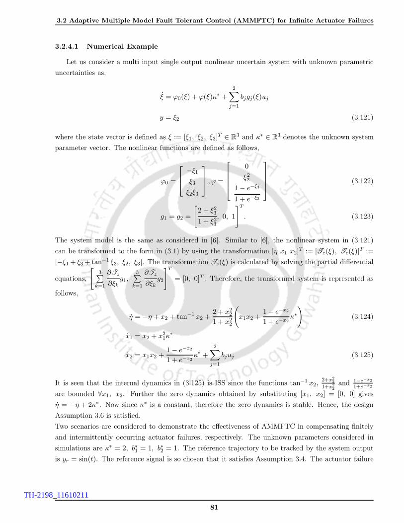
3.2 Adaptive Multiple Model Fault Tolerant Control (AMMFTC) for Infinite Actuator Failures
3.2.4.1 Numerical Example
Let us consider a multi input single output nonlinear uncertain system with unknown parametric
uncertainties as,
ξ = ϕ0(ξ) + ϕ(ξ)κ∗ +2∑
j=1
bjgj(ξ)uj
y = ξ2 (3.121)
where the state vector is defined as ξ := [ξ1, ξ2, ξ3]T ∈ R
3 and κ∗ ∈ R3 denotes the unknown system
parameter vector. The nonlinear functions are defined as follows,
ϕ0 =
−ξ1ξ3
ξ2ξ3
, ϕ =
0
ξ221 − e−ξ3
1 + e−ξ3
(3.122)
g1 = g2 =
[2 + ξ23
1 + ξ23, 0, 1
]T. (3.123)
The system model is the same as considered in [6]. Similar to [6], the nonlinear system in (3.121)
can be transformed to the form in (3.1) by using the transformation [η x1 x2]T := [Tz(ξ), Tc(ξ)]
T :=
[−ξ1 + ξ3 + tan−1 ξ3, ξ2, ξ3]. The transformation Tz(ξ) is calculated by solving the partial differential
equations,
[3∑
k=1
∂Tz
∂ξkg1,
3∑k=1
∂Tz
∂ξkg2
]T= [0, 0]T . Therefore, the transformed system is represented as
follows,
η = −η + x2 + tan−1 x2 +2 + x2
2
1 + x22
(x1x2 +
1 − e−x2
1 + e−x2κ∗)
(3.124)
x1 = x2 + x21κ
∗
x2 = x1x2 +1 − e−x2
1 + e−x2κ∗ +
2∑
j=1
bjuj (3.125)
It is seen that the internal dynamics in (3.125) is ISS since the functions tan−1 x2,2+x2
2
1+x22
and 1−e−x2
1+e−x2
are bounded ∀x1, x2. Further the zero dynamics obtained by substituting [x1, x2] = [0, 0] gives
η = −η + 2κ∗. Now since κ∗ is a constant, therefore the zero dynamics is stable. Hence, the design
Assumption 3.6 is satisfied.
Two scenarios are considered to demonstrate the effectiveness of AMMFTC in compensating finitely
and intermittently occurring actuator failures, respectively. The unknown parameters considered in
simulations are κ∗ = 2, b∗1 = 1, b∗2 = 1. The reference trajectory to be tracked by the system output
is yr = sin(t). The reference signal is so chosen that it satisfies Assumption 3.4. The actuator failure
81
TH-2198_11610211

3. Adaptive Multiple Model Fault Tolerant Control (AMMFTC) of Nonlinear UncertainSystems with Actuator Failures
model representing Scenario 1 , is defined as follows,
u1(t) =
5, t ∈ [50, 100)
uH1(t), t ∈ [0, 50) ∪ [100, ∞), u2(t) =
uH2(t), t ∈ [0, 100) (3.126)
Further, the intermittently occurring actuator fault/failure considered in Scenario 2 is described in
(3.127) below.
u1(t) = uFj1,h, t ∈ [hT ∗, (h+ 1)T ∗), h ∈ N\2N (3.127)
The transition time between each change in the actuator failure pattern is considered to be T ∗ = 5 > 0.
The value at which the actuator gets stuck corresponding to Scenario 2 is given by uFj1,h = 5. The
bounds on the unknown parameters are given below.
1 ≤ κ∗ ≤ 3, 0.8 ≤ |b∗1| ≤ 1.4, 0.6 ≤ |b∗2| ≤ 2 (3.128)
0.5 ≤ Kj,h ≤ 1, |uFjk,h| ≤ 6, j = 1, 2. (3.129)
Hence, Assumptions 3.2 and 3.5 also hold. The initial conditions of the system are given by ξ(0) =
[0, 0.4, 0]. The adaptive controller is designed using the AMMFTC methodology discussed in Section
3.3.2. The number of unknown parameters being 4, we choose N = 5 adaptive identifiers so that
the initial parameter vector estimates from each of the identification models form a convex hull. The
initial parameter estimates from each of the N estimators are θ(1)(0) = [1, 1, 0, 0]T , θ(2)(0) =
[1.5, 2.5, 6, 6]T , θ(3)(0) = [2.5, 1, 0, 0]T , θ(4)(0) = [2.5, 2.5, −6, −6]T , θ(5)(0) = [2, 1.5, 0, 0]T .
The controller design parameters for simulation are chosen to be c1 = c2 = 5, c1 = c2 = 3, g2 =
3, γ = 0.5, Γ1 = Γ2 = Γ3 = Γ4 = Γ5 = 40 × I2 and A0 = [diag(−5, −7)]. In order to provide a
fair comparison of the proposed control design with single model adaptive control and the modular
backstepping control (MBSC) approach by Wang et. al [6], the values of controller gains and other
relevant design parameters are chosen to be same. The output performance in regards to start-up and
post fault transient peaks and settling times, is calculated using root mean square (RMS) and integral
time absolute error (ITAE) metric of the output tracking error. A relatively lower value of ITAE and
RMSE from the results obtained with other relevant control schemes, signify a faithful tracking with
comparatively lower overshoots and faster settling time. Further, the input performance is quantified
using control energy (CE) and the total variation (TV) of the control signal. Total variation is a very
important measure which gives an insight on the frequency of input usage. The lower the value of TV
and CE, better is the input performance. The control energy is measured using the 2−norm of the
control input whereas TV for each of the control inputs is measured using the expressionN∑i=1
|uj,i−uj,i+1|for j = 1, 2.
• Scenario 1 (3.126): Under no fault conditions, the output tracking performance, the convergence
of parameter estimates along with the remaining system states and the control signals are shown
in Figures 3.5 and 3.6, respectively. As proved in the theoretical analysis earlier, fastness of
parameter convergence and improvement in output transient performance using the proposed
82
TH-2198_11610211

3.2 Adaptive Multiple Model Fault Tolerant Control (AMMFTC) for Infinite Actuator Failures
Time [s]0 5 10 15 20 25
‖x1−
yr‖
0
0.05
0.1
0.15
0.2
0.25
0.3
0.35
0.4Norm of tracking error
MBSCSingle ModelMultiple Model
Time [s]0 5 10 15 20 25
‖θ‖
0
1
2
3
4
5
6
7
8
9Norm of parameter estimation error
MBSCSingle ModelMultiple Model
Figure 3.5: Comparison of start-up output transient performance and parameter convergence obtained with ModularBackstepping Control (MBSC) [6], single model adaptive control and proposed multiple model adaptive control
controller are clearly evident from Figure 3.5. The proposed controller using multiple models
exhibits a superior output performance compared to a single model adaptive control scheme and
modular backstepping control (MBSC) [6] without significantly increasing the control energy.
Further, in the event of an abrupt actuator failure at t = 50 s, the proposed control methodology
retains similar beneficial attributes in terms of rapid accommodation of actuator failure and fast
post failure output tracking with minimal overshoots. The above inference is drawn from the
simulation results provided in Figures 3.7 and 3.8. In addition, a consolidated performance chart
summarizing the efficacy of the proposed controller relative to relevant existing adaptive control
techniques is furnished in Table 3.1.
Table 3.1: Tabular comparison of output and input performance under Scenario 1 (3.126).
Control SchemesOutput Performance Input Performance
ITAE RMSEControl Energy Total Variation
u1 u2 u1 u2
Multiple Models 18.69 0.0134 3.644 × 10³ 3.126 × 10³ 131.72 297.48Single Model 49.83 0.0268 3.643 × 10³ 3.102 × 10³ 147.78 305.48MBSC 34.64 0.0195 3.639 × 10³ 3.106 × 10³ 127.97 286.34
• Scenario 2 (3.127): This scenario demonstrates the robustness of the proposed adaptive controller
to intermittently changing actuator failure patterns unknown in time, pattern and magnitude.
The value at which u1 is stuck is uFj1 = 5. These eventualities are manifested in the form of
infinitely occurring parameter jumps which are uncertain and unknown in all aspects except for
83
TH-2198_11610211

3. Adaptive Multiple Model Fault Tolerant Control (AMMFTC) of Nonlinear UncertainSystems with Actuator Failures
Time [s]0 10 20 30 40 50
Out
put y
= ξ 2
-1
-0.5
0
0.5
1
1.5
ξ2 yr
(a)
Time [s]0 10 20 30 40 50
ξ 1
-2
-1
0
1
2
3
4
(b)
Time [s]0 10 20 30 40 50
ξ 3
-2.5
-2
-1.5
-1
-0.5
0
0.5
1
1.5
(c)
Time [s]0 10 20 30 40 50
Con
trol
inpu
ts
-2
0
2
4
6
8
u1
u2
(d)
Figure 3.6: System states and control input with no actuator fault under Scenario 1 (3.126) from t = 0 ∼ 50 s. (a)Output state ξ2 = x1;(b) state ξ1;(c) state ξ3 = x2; (d) control inputs u1 and u2
the boundary set they reside in. Figure 3.10 shows the boundedness of all the system states
and the control signals under this scenario with the transit time being T ∗ = 5 s. Further, the
theoretical result claiming the improvement of output transient performance with an increasing
T ∗, is verified from the simulation results obtained with T ∗ = 5 s and T ∗ = 15 s in Figure
3.9 along with performance measures tabulated in Table 3.2. The superior features of the pro-
posed adaptive control methodology are concluded from the tabulation of input and output
performances obtained using the proposed method, single model adaptive control and modular
adaptive backstepping control (MBSC) [6] techniques in Table 3.2.
84
TH-2198_11610211

3.2 Adaptive Multiple Model Fault Tolerant Control (AMMFTC) for Infinite Actuator Failures
Time [s]50 60 70 80 90 100
‖x1−
yr‖
0
0.01
0.02
0.03
0.04
0.05
0.06
0.07Norm of tracking error
Multiple ModelSingle ModelMBSC
Time [s]50 60 70 80 90 100
‖θ‖
0
0.5
1
1.5
2
2.5
3
3.5
4Norm of parameter estimation error
Multiple ModelSingle ModelMBSC
Figure 3.7: Scenario 1. Comparison of post-failure output transient performance and parameter convergence obtainedwith Modular Backstepping Control (MBSC) [6], single model adaptive control and proposed multiple model adaptivecontrol
Table 3.2: Tabular comparison of output and input performance for Scenario 2 (3.127) describing infinite actuator failureswith T ∗ = 5 s and T ∗ = 15 s
Transit time Control SchemesPerformance metrics
ITAE RMSEControl Energy Total Variation
u1 u2 u1 u2
T ∗ = 5 sMultiple Models 78.46 0.023 3.64 × 10³ 3.09 × 10³ 293.64 359.15Single Model 124.44 0.039 3.74 × 10³ 3.22 × 10³ 309.69 380.27MBSC 111.08 0.032 3.67 × 10³ 3.14 × 10³ 291.05 362.00
T ∗ = 15 sMultiple Models 56.10 0.018 3.48 × 10³ 2.99 × 10³ 180.41 299.11Single Model 85.75 0.033 3.47 × 10³ 2.93 × 10³ 200.45 319.21MBSC 62.93 0.026 3.47 × 10³ 2.94 × 10³ 181.15 327.89
85
TH-2198_11610211

3. Adaptive Multiple Model Fault Tolerant Control (AMMFTC) of Nonlinear UncertainSystems with Actuator Failures
Time [s]0 20 40 60 80 100
Out
put y
= ξ 2
-1.5
-1
-0.5
0
0.5
1
1.5
2
ξ2 yr
(a)
Time [s]0 20 40 60 80 100
ξ 1
-3
-2
-1
0
1
2
3
4
(b)
Time [s]0 20 40 60 80 100
ξ3
-2.5
-2
-1.5
-1
-0.5
0
0.5
1
1.5
(c)
Time [s]0 20 40 60 80
Con
trol
inpu
ts
-10
-8
-6
-4
-2
0
2
4
6
8u1 u2
(d)
Figure 3.8: System states and control inputs with actuator fault under Scenario 1 (3.126) at t = 50 s. (a) Output stateξ2 = x1;(b) state ξ1;(c) state ξ3 = x2; (d) control inputs u1 and u2
3.2.4.2 Application to an Aircraft System
In this section, a problem of longitudinal control of Boeing 747-100/200, a large transport aircraft
is considered. It is assumed that the aircraft is subjected to infinite number of PLOE and LIP elevator
failures at unknown time instants. This example would further demonstrate the applicability and
proficiency of the proposed multiple model adaptive control scheme to practical systems. The aircraft
model parameters chosen for simulations along with their respective notations and definitions are
provided in Section 2.2.5. The longitudinal control dynamics of the aircraft can be referred to (2.57)-
(2.58) and is not repeated here for brevity. The state variables are chosen as [x1, x2, x3, x4]T =
86
TH-2198_11610211

3.2 Adaptive Multiple Model Fault Tolerant Control (AMMFTC) for Infinite Actuator Failures
Time [s]0 20 40 60 80 100
‖x1−yr‖
0
0.05
0.1
0.15
0.2
0.25
0.3
0.35
0.4Norm of tracking error (T∗=5)
Time [s]0 20 40 60 80 100
‖x1−yr‖
0
0.05
0.1
0.15
0.2
0.25
0.3
0.35
0.4Norm of tracking error (T∗=15)
30 35 40 45 50 55
0
0.05
0.1
MBSCSingle ModelMultiple Model
30 35 40 45 50 55
0
0.05
0.1
0.15
MBSCSingle ModelMultiple Model
Figure 3.9: Comparison of post failure transient performance obtained with Modular Backstepping Control (MBSC),single model adaptive control and proposed multiple model adaptive control in case of infinite actuator failures
[V, α, θ, q]T and u1 = δe1 , u2 = δe2 are the control inputs. The system dynamics required for control
design, are as follows,
x3 = x4 (3.130)
x4 = a(x, η) + a(x, η)κ∗ +m∑
j=1
bjβj(ξ, η)uj (3.131)
where κ∗ ∈ R models the unknown factor of additive uncertainty in system dynamics. It basically
denotes the deviation of the actual system model from its nominal model dynamics. The actuator
failure model considered for the elevators is as follows,
u1(t) = uFj1,h, u2(t) = K2,huH2 t ∈ [hT ∗, (h+ 1)T ∗), h ∈ N\2N (3.132)
The above failure characteristics of the actuator assumes T ∗ = 10, the value at which the actuator
is stuck uFj1,h = 2 and the LOE factor K2,h = 0.7. Therefore, it is observed that the actuators
switch from their healthy state of operation to a faulty state at each time interval of 10 s. The
bounds on the unknown model and fault parameters are, |κ∗| ≤ 1, 0.5 ≤ |bj| ≤ 2, 0.2 ≤ Kj,h ≤ 1
and uFj,h ≤ 5, j = 1, 2. The initial state vector is considered to be [0.0162, 230, 0.0162, 0]T and
w(t0) = [0.25, 0.25, 0.25, 0.25]T . The reference signal for tracking is given by yr = 0.1 sin(0.05t). The
controller design parameters are given as follows: c1 = 30, c2 = 1, c1 = 0.1, c2 = 0.5, g2 = 10−6 and
ℓ = 0.01. The observer design matrix A0 = 5I2×2 and adaptive rate matrix Γ1 = Γ2 = Γ3 = Γ4 = 2I2×2
are considered in simulations. The number of models considered is N = 4. The minimum number
of estimators are selected so as to satisfy that the set θ(µ)(t0)Nµ=1 forms a convex hull ∀t ≥ t0.
87
TH-2198_11610211

3. Adaptive Multiple Model Fault Tolerant Control (AMMFTC) of Nonlinear UncertainSystems with Actuator Failures
Time [s]0 20 40 60 80 100
Out
put y
= ξ 2
-1.5
-1
-0.5
0
0.5
1
1.5
2
ξ2 yr
(a)
Time [s]0 20 40 60 80 100
Sta
te ξ 1
-3
-2
-1
0
1
2
3
4
(b)
Time [s]0 20 40 60 80 100
Sta
te ξ 3
-2.5
-2
-1.5
-1
-0.5
0
0.5
1
1.5
(c)
Time [s]0 20 40 60 80 100
Con
trol
inpu
ts
-20
-15
-10
-5
0
5
10
u1 u2
(d)
Figure 3.10: System states and control inputs with intermittent actuator fault/failures under Scenario 2 (3.127). (a)Output state ξ2 = x1;(b) state ξ1;(c) state ξ3 = x2; (d) control inputs u1 and u2
Therefore, the initial parameter set is constructed using the initial parameter estimates from each of
the N models defined as θ(1)(t0) = [1, 0.4, 5]T , θ(2)(t0) = [−1, 3, −5]T , θ(3)(t0) = [1, 0.4, −5]T and
θ(4)(t0) = [−1, 3, 5]T , respectively. Similar to the simulation illustration of the numerical example
considered, the output transient and steady state performance is evaluated on the basis of ITAE and
RMSE.
The simulation results obtained are provided in Figures 3.11 and 3.12. In such an event of infinitely
occurring actuator failures, the boundedness of all the closed loop signals, namely, the pitch angle
θ, pitch rate q, the angle of attack (AoA) α and velocity V along with the control inputs using the
88
TH-2198_11610211

3.2 Adaptive Multiple Model Fault Tolerant Control (AMMFTC) for Infinite Actuator Failures
Time [s]0 20 40 60 80 100
‖x3−
yr‖
×10-3
0
2
4
6
8
10
12
14
16
18Norm of tracking error
10 20 30 40 50 60
×10-4
0
0.5
1
1.5 MBSCSingle ModelMultiple Model
Time [s]0 0.5 1 1.5 2 2.5 3
‖x3−
yr‖
×10-3
0
2
4
6
8
10
12
14
16
18Norm of tracking error (start up)
MBSCSingle ModelMultiple Model
Figure 3.11: Comparison of start up and post failure transient performance obtained with Modular Backstepping Control(MBSC), single model adaptive control and multiple model adaptive control in case of infinite actuator failures
proposed adaptive controller is shown in Figure 3.12. Similar to the example considered in the previous
section, the transient at start up and post failure in addition to the steady state behavior of the output
is compared with those obtained using a single model adaptive controller and modular backstepping
control (MBSC) [6]. For the sake of a fair comparison, all the relevant design parameters for all the
three controllers are said to take identical values. The initial condition for the parameter estimate θ
in single model adaptive control and MBSC are taken to be θ(t0) = [−1, 3, 5]T whereas the plant
initial conditions are x(t0) = [0.794, 230, 0.0162, 0]T . The results in Figure 3.11 unveils the superior
convergence of the tracking error norm compared to adaptive control using a single model and MBSC
in terms fastness and accuracy of tracking. Quantitatively, the performance improvement is reflected
from the ITAE and RMSE of the output tracking error at start up using each of the three control
schemes. The ITAE values for the proposed method, single model adaptive control are recorded to be
0.00082 and 0.0898, respectively. Whereas, their RMSE measurements are calculated to be 0.00033
and 0.0079, respectively. Further, the enhanced performance for all time 0 ≤ t < ∞ is evident from
the zoomed figure in Figure 3.11.
Remark 3.4. From extensive simulations, it has been observed that the performance of the proposed
control scheme is directly proportional to the choice of sampling frequency. Further, a judicious low-
ering of the sampling frequency while maintaining boundedness of the closed loop signals, impacts the
performance of the proposed control design. Nevertheless, the magnitude of impact on performance due
to increment in sampling time, is relatively insignificant compared to results obtained in simulation
studies using adaptive control with single models and MBSC. For example, the MBSC based control
system with the aircraft example renders a faithful performance with a sampling interval of 0.0001
s. While, a similar or rather a better performance is achieved utilizing the proposed multiple model
89
TH-2198_11610211

3. Adaptive Multiple Model Fault Tolerant Control (AMMFTC) of Nonlinear UncertainSystems with Actuator Failures
Time [s]0 20 40 60 80 100
Trackingerrorx3−yr
-0.03
-0.02
-0.01
0
0 20 40 60 80 100
×10-4
-4
-2
0
2
4
(a)
Time [s]0 20 40 60 80 100
Pitc
h an
gle θ
= x
3
-0.1
-0.05
0
0.05
0.1
0.15
θ = x3yr
(b)
Time [s]0 20 40 60 80 100
Pitch
rate
q=
x4
-0.01
-0.005
0
0.005
0.01
q
yr
(c)
Time [s]20 40 60 80 100
Con
trol
inpu
ts
-4
-2
0
2
4
6
8
10
12
u1 u2
(d)
Figure 3.12: (a) aircraft pitch angle tracking error;(b) actual and desired aircraft pitch angle θ = x3; (c) aircraft pitchrate x4; (d) control inputs u1 and u2;
adaptive control scheme with a sampling time of 0.005 s. Hence, it can be concluded, that the proposed
algorithm is efficient and suitable for real time applications with limited bandwidth.
3.3 Adaptive Multiple Model Fault Tolerant Control (AMMFTC)
for Uncertain Multi-Input-Multi-Output (MIMO) Nonlinear Sys-
tems
In what follows, the proposed multiple model adaptive control strategy is further applied to solve the
FTC design problem in nonlinear uncertain MIMO systems. Incorporating the event of occurrence of
abrupt uncertain actuator failures into the underlying system dynamics leads to several challenges in an
effective control design. Apart from unknown system uncertainties and being affected by unanticipated
90
TH-2198_11610211

3.3 Adaptive Multiple Model Fault Tolerant Control (AMMFTC) for UncertainMulti-Input-Multi-Output (MIMO) Nonlinear Systems
actuator faults and external perturbations, these systems inherently exhibit strong coupling effects
between each of their subsystems. Withal, adaptive fault tolerant controller synthesis for such coupled
MIMO nonlinear systems to effectively compensate actuator failures is indeed challenging. In the
following, the FTC design problem for MIMO nonlinear systems affected by actuator failures, system
uncertainties and unknown subsystem interactions is formulated and thereafter a control solution is
derived.
3.3.1 Problem Formulation
Let us consider a MIMO nonlinear system as follows,
∑p:
x = f0(x) +p∑i=1
κ∗i fi(x) +m∑j=1
gj(x)uj
y = h(x)
(3.133)
The state vector of the system (3.133) is denoted by x := [x1, x2, . . . , xn]T ∈ R
n. The vector y :=
[y1, y2, . . . , yq]T ∈ R
q represents the outputs while h(x) are defined as known smooth functions.
Further, f0, fi,gj : Rn → R
n represent the vectors of known smooth nonlinear functions for i = 1, . . . , n
and j = 1, . . . ,m. The terms uj defines the control inputs, collectively denoted by the vector u :=
[u1, u2, . . . , um]T and κi, i = 1, . . . , p are unknown constants.
Considering the system dynamics in (3.133), the following assumptions are necessary.
Assumption 3.7. The system (3.133) has well defined relative degrees ℘ = ℘1, ℘2, . . . , ℘q, 1 ≤℘i ≤ n, for i = 1, 2, . . . , n. Therefore the following equalities hold for j = 1,m, i = 1, q and
k = 0, ℘i − 2.
LgjLkf0hi(x) = 0, LgjL
℘i−1f0
hi(x) 6= 0
The operator Lf (·) defines the Lie derivative of the argument in the direction of f(x). Further, the
nonlinear functions fi satisfy the conditions given below [102] for k = 1, p, ri = 1, ℘i − 1 and i = 1, q,
Dx(LfkLri−1f0
hi(x)) ∈ spanDx(h1(x)), . . . ,Dx(L℘1−℘i+ri−1f0
h1(x)),Dx(h2(x)), . . . ,Dx(L℘2−℘i+ri−1f0
h2(x)),
Dx(hj(x)), . . . ,Dx(L℘j−℘i+ri−1f0
hj(x)),Dx(hq(x)), . . . ,Dx(L℘q−℘i+ri−1f0
hq(x)),
where, the operator Dx(·) denotes the partial differentiation of a function with respect to x ∈ Rn
resulting in a gradient vector Dx(·) :=
[∂
∂x1,
∂
∂x2, . . . ,
∂
∂xn
]T(·).
In accordance with FTC literature, actuator fault in a system manifests itself in either of the forms
as under, (i) partial loss of effectiveness (PLOE);(ii) lock-in-place (LIP);(iii) float failure. However in
this work, LIP and float failures have been considered. Such types of actuator faults can be charac-
terized by a unified mathematical model with a piecewise defined input-output relationship as given
91
TH-2198_11610211
3. Adaptive Multiple Model Fault Tolerant Control (AMMFTC) of Nonlinear UncertainSystems with Actuator Failures
below [100].
uj =
KjuHj + uFj,
uHj,
∀ t ≥ tFj
∀ t < tFjj = 1,m (3.134)
The term uHj and uFj denote the controller output fed to the jth actuator and the value at which the
jth actuator is stuck under LIP failure, respectively. Float failure is the condition when the jth actuator
fails with uFj=0. Apart from the additive consequences of actuator failures, multiplicative actuator
faults are modeled using the factor Kj . The actuator failure value uFj, the actuation effectiveness
index Kj , the failure time instant tFj and the actuator index j are all unknown. This means that the
actuator failures are unknown in time, pattern as well as magnitude. The actuator index set is given
by j1, j2, . . . , jm. Unlike the actuator fault modeling in multi-input single-output (MISO) systems
wherein the actuators were assumed to have same/similar physical characteristics, MIMO systems
have multiple inputs with actuators not necessarily reflecting the same physical behavior/features and
functioning. Therefore, to design fault tolerant controllers for a MIMO nonlinear system, an actuator
grouping scheme G := G1, G2, . . . ,Gq is required [32]. Herein, each set Gk ⊂ j1, j2, . . . , jmrepresents the set of actuators with similar operational characteristics and such a classification is done
on the basis of ℘ := ℘1, ℘2, . . . , ℘q. Further to effectively exploit the actuator redundancy, a
proportional actuation scheme is utilized similar to [32]. Therefore, considering such a grouping and
actuation scheme G , the control input to be fed to each actuator included in the set Gk is given by,
uHj = bjkvk ∀uj ∈ Gk, j = 1, m & k = 1, q (3.135)
where, bjk defines a certain design function associated with each actuator group Gk. Further, the choice
of such design functions satisfy the relation bjk = bj if the jth actuator belong to Gk under the grouping
scheme G . Thereafter, to facilitate control design, under assumption 3.7 and (3.133)-(3.135), there ex-
ists a diffeomorphism T (x) := [ξ,η]T = [ξ1,1, ξ1,2, . . . , ξ1,℘1, . . . , ξq,1, ξq,2, . . . , ξq,℘q ,η] = [Tc(x),Tz(x)]T
such that
Tc(x) := [h1(x), Lf0h1(x), . . . , L℘1−1f0
h1(x), . . . , hq(x), Lf0hq(x), . . . , L℘q−1f0
hq(x)] ∈ R℘1+℘2+...+℘q
and Tz ∈ Rℓ transforms the system (3.133) to the following form with a controllable part
∑c and
internal dynamics∑
z,
∑c1
:
ξ1,r1 = ξ1,r1+1 +ϕT1,r1κ∗
ξ1,℘1 = a1(ξ, η) +ϕT1,℘1κ∗ +
∑j∈j1,...,jd
β1,j(ξ, η)uFj +q∑
k=1
β1,k(ξ, η)vk(3.136)
92
TH-2198_11610211

3.3 Adaptive Multiple Model Fault Tolerant Control (AMMFTC) for UncertainMulti-Input-Multi-Output (MIMO) Nonlinear Systems
...
∑cq
:
ξq,rq = ξq,rq+1 +ϕTq,rqκ∗
ξq,℘q = aq(ξ, η) +ϕTq,℘qκ∗ +
∑j∈j1,...,jd
βq,j(ξ, η)uFj +q∑
k=1
βq,k(ξ, η)vk(3.137)
∑z
: η = Λ0(ξ,η) + ΛT1 (ξ,η)κ∗ + ΛT
2 (ξ,η)u (3.138)
y = [ξ1,1, ξ2,1, ξ3,1, . . . , ξi,1, . . . , ξq,1]T (3.139)
where ϕi,ri(ξ,η) := [Lrif1hi(x), . . . , Lri
fphi(x)]T , ai(ξ,η) := L℘i
f0hi(x), βi,j(ξ,η) := LgjL
℘i−1f0
hi(x),
βi(ξ,η) := [LgjL℘i−1f0
hi(x)mj=1], βi,k :=∑
j 6∈j1,...,jd∩Gk
bjkKjβi,j(ξ,η) ∀k = 1, . . . , q
Λ0(ξ,η) := ∂Tz∂x f0(x), ΛT
1 (ξ,η) :=∂Tz
∂x[f1(x), f2(x), . . . , fp(x)] and
ΛT2 (ξ,η) :=
∂Tz
∂x[g1(x), g2(x), . . . , gm(x)] for i = 1, q, ri = 1, ℘i − 1 and j = 1,m. At this point, we
are well equipped to state the following additional assumptions.
Assumption 3.8. The zero dynamics (3.138) of the system (3.133), given by∑z
:= Λ0(ξ,η) +
ΛT1 (ξ,η)κ∗ + ΛT
2 (ξ,η)u is input-to-state-stable (ISS) for each failure pattern with ξ as the input.
With a supposition that there are M possible actuator failure patterns, the equivalent actuation matrix
given by the argument of det operator in (3.140), for the entire system corresponding to an actuator
failure pattern Ξ ∈ Ξ, = 1,M under the grouping scheme G should be non-singular ∀x ∈ Rn, that
is,
det
∑j 6∈j1,...,jd∩G1
bj1KjLgjL℘1−1f0
h1(x) . . .∑
j 6∈j1,...,jd∩Gq
bjqKjLgjL℘1−1f0
h1(x)
∑j 6∈j1,...,jd∩G1
bj1KjLgjL℘2−1f0
h2(x) . . .∑
j 6∈j1,...,jd∩Gq
bjqKjLgjL℘2−1f0
h2(x)
.... . .
...∑
j 6∈j1,...,jd∩G1
bj1KjLgjL℘q−1f0
hq(x) . . .∑
j 6∈j1,...,jd∩Gq
bjqKjLgjL℘q−1f0
hq(x)
G (Ξ)
6= 0.
(3.140)
Herein, Ξ defines a set with cardinality M =(mq
), whose elements are m × m diagonal matrices
representing all possible actuator failure topologies. Further, the diagonal elements of each of such
matrices in Ξ are either zero or unity depending on the state of health of the corresponding actuator. It
is to be mentioned at this point in time that all of the M actuator failure patterns are not compensable
and hence it is required to classify failures as compensable and non-compensable ones. The basis of
such a classification are the actuation matrices corresponding to all possible failure topologies. The non-
singularity of the actuation matrix for an actuator failure pattern is the deciding factor which defines
an actuator failure pattern to be compensable or not. In other words, this classification criterion, if
satisfied, guarantees the existence of an adaptive fault tolerant controller which can ensure stability of
the closed-loop system in the event of actuator failures.
93
TH-2198_11610211

3. Adaptive Multiple Model Fault Tolerant Control (AMMFTC) of Nonlinear UncertainSystems with Actuator Failures
Assumption 3.9. The nonlinear dynamical system in (3.133) is so designed that the desired output
performance can only be achieved in the event of atmost d ≤ (m − q) actuator failures unknown in
time, pattern and magnitude. Further, under the grouping scheme G , since the actuators are grouped
on the basis of their similarity in structural characteristics, atleast one actuator in each of the groups
Gk should be operational corresponding to an actuator failure pattern.
Assumption 3.10. The respective reference trajectories yr(t) := [yr,1, yr,2, . . . , yr,q]T ∈ R
q to be
tracked by the system outputs are known, piecewise continuous and bounded. Further, yr, yr, . . . ,y(℘)r ∈
Rq are also piecewise continuous, bounded and belong to a known compact set.
Having stated all the necessary definitions and assumptions, we are now well equipped to state the
FTC design problem. Considering the nonlinear uncertain MIMO system (3.133) and the assumptions
3.7-3.10, the control problem and its objectives can be framed as follows:
• To design the control inputs vk corresponding to each actuator group Gk for k = 1, q such that
the closed loop system is stable and the output vector y(t) tracks the desired reference vector
yr(t) in the event of atmost d ≤ (m − q) unknown actuator failures ∀ t ∈ [0, ∞). The design
assumes no prior knowledge of the magnitude, pattern and time tjF of the occurrence of actuator
failures/faults.
• To ensure an improved start-up and post failure output transient performance without any sig-
nificant expense of control energy
• Asymptotic stability of output tracking error vector, i.e. limt→∞
y(t) − yr(t) = 0 under no failure
and past fault scenarios.
• Guaranteeing robustness towards parametric uncertainties, external perturbations and conse-
quences of strong unknown cross coupling arising from subsystem interactions through estimation
and subsequent compensation instead of merely alleviating their adverse effects.
3.3.2 Adaptive Multiple Model Fault Tolerant Control (AMMFTC) Design
Referring to the transformed system dynamics in (3.137)-(3.138), to simplify the control design
procedure, the unknown system and failure induced parameters are denoted as θ∗2 = κ∗, θ∗1 =
[θ∗1,1, . . . , θ∗1,m]T = [Kjmj=1]
T and θ∗3 = [θ∗3,1, . . . , θ∗3,m]T = [uFjmj=1]
T . Further, the overall un-
known parameter vector is defined as θ∗ := [θ∗1 , θ∗2, θ
∗3]T . The control design procedure follows
similar steps as discussed in Section 3.2.2 wherein the same control design problem was considered for
single output nonlinear systems with operationally similar multiple inputs. Firstly, we proceed with
an input-state-stable (ISS) controller design assuming the availability of parameter estimates from a
faithful parameter estimator to ensure modularity between the controller-observer pair. Thereafter,
the proposed multiple model parameter estimator is constructed to yield the parameter estimates to be
fed to the controller for subsequent compensation preserving closed loop system stability ∀ t ∈ [0, ∞).
94
TH-2198_11610211

3.3 Adaptive Multiple Model Fault Tolerant Control (AMMFTC) for UncertainMulti-Input-Multi-Output (MIMO) Nonlinear Systems
3.3.2.1 Controller Synthesis
For simplicity and ease of understanding, the control design is explained following a stepwise
procedure as given below.
Step 1.1: Let us choose the first output error variable as z1,1 = y1 − yr,1 = ξ1,1 − yr,1. Further, define
z1,2 = ξ1,2 − α1,1 − yr,1 and θ := θ∗ − θ. Where αi,ri with ri = 1, ℘i are stabilizing input functions for
each of the subsystems incurred during control design. The error dynamics are given by,
z1,1 = ξ1,2 +ϕT1,1θ∗2 − yr,1 (3.141)
= z1,2 + α1,1 + yr,1 (3.142)
The first virtual control law α1,1 is so chosen as to stabilize the z1,1 dynamics and is defined as follows,
α1,1 = −c1,1z1,1 − c1,1‖ψ1,1‖2z1,1 −ϕT1,1θ2 (3.143)
Substituting α1,1 from (3.143) in (3.142) results in,
z1,1 = −c1,1z1,1 − c1,1‖ψ1,1‖2z1,1 + z1,2 +ϕT1,1(θ∗2 − θ2) (3.144)
Step 1.r1: For r1 = 2, ℘1 − 1, the steps of control design are similar wherein the rth1 error variable is
chosen as z1,r1 := ξ1,r1 − α1,r1−1 − y(r1−1)r,1 . Therefore,
z1,r1 = ξ1,r1+1 +ϕT1,r1θ∗2 −
r1−1∑
k=1
∂α1,r1−1
∂ξ1,kϕT1,kθ
∗2 −
∂α1,r1−1
∂θ2
˙θ2 −
r1−1∑
k=1
∂α1,r1−1
∂ξ1,kξ1,k+1 −
r1−1∑
k=1
∂α1,r1−1
∂yk−1r,1
y(k)r,1
= z1,r1+1 + α1,r1 +
(ϕT1,r1 −
r1−1∑
k=1
∂α1,r1−1
∂ξ1,kϕT1,k
)
︸ ︷︷ ︸ψ1,r1
θ∗2 −∂α1,r1−1
∂θ2
˙θ2
−(r1−1∑
k=1
∂α1,r1−1
∂ξ1,kξ1,k+1 +
r1−1∑
k=1
∂α1,r1−1
∂yk−1r,1
y(k)r,1
)(3.145)
To stabilize the above subsystem (3.145), the virtual control law α1,r1 is formulated to be,
α1,r1 = −z1,r1−1 − c1,r1z1,r1 − c1,r1‖ψ1,r1‖2z1,r1 − g1,r1
∥∥∥∥∥∂α1,r1−1
∂θ2
∥∥∥∥∥
2
z1,r1 −ψT1,r1θ2
+
(r1−1∑
k=1
∂α1,r1−1
∂ξ1,kξ1,k+1 +
r1−1∑
k=1
∂α1,r1−1
∂yk−1r,1
y(k)r,1
)(3.146)
95
TH-2198_11610211

3. Adaptive Multiple Model Fault Tolerant Control (AMMFTC) of Nonlinear UncertainSystems with Actuator Failures
Such a choice of the stabilizing functions at the rth1 step yields,
z1,r1 = −z1,r1−1 + z1,r1+1 − c1,r1z1,r1 −
c1,r1‖ψ1,r1‖2 + g1,r1
∥∥∥∥∥∂α1,r1−1
∂θ2
∥∥∥∥∥
2
z1,r1
− ∂α1,r1−1
∂θ2
˙θ2 +ψT1,r1(θ
∗2 − θ2) (3.147)
Step i.ri: Following similar steps as detailed in the immediately preceding text for the error variables,
z2,1, z2,2, . . . , z2,℘2−1, . . . , zq,1, zq,2, . . . , zq,℘q−1, where
zi,1 = yi − yr,i = ξi,1 − yr,i; i = 2, . . . , q (3.148)
zi,ri = ξi,ri − αi,ri−1 − y(ri−1)r,i ; ri = 2, . . . , ℘i − 1 (3.149)
the virtual control laws αi,ri are obtained as given below satisfying the input-to-state-stable(ISS)
criterion with respect to zi,ri+1 as the input.
α2,1 = −c2,1z2,1 − c2,1‖ψ2,1‖2z2,1 −ϕT2,1θ2 (3.150)
αi,ri = −zi,ri−1 − ci,rizi,ri −
ci,ri‖ψi,ri‖2 + gi,ri
∥∥∥∥∥∂αi,ri−1
∂θ2
∥∥∥∥∥
2
zi,ri −ψTi,riθ2
+
(ri−1∑
k=1
∂αi,ri−1
∂ξi,kξi,k+1 +
ri−1∑
k=1
∂αi,ri−1
∂yk−1r,i
y(k)r,i
)(3.151)
In the expression for αi,ri for ri = 2, ℘i − 1, the regressor term ψi,ri(·) is defined as
ψi,ri = ϕi,ri −ri−1∑
k=1
∂αi,ri−1
∂ξi,kϕi,k.
Therefore, with the above choice of αi,ri , the dynamics of zi,ri for i = 2, . . . , q are described as,
z2,1 = −c2,1z2,1 − c2,1‖ψ2,1‖2z2,1 + z2,2 +ϕT2,1(θ∗2 − θ2) (3.152)
......
zi,ri = −zi,ri−1 + zi,ri+1 − ci,rizi,ri −
ci,ri‖ψi,ri‖2 + gi,ri
∥∥∥∥∥∂αi,ri−1
∂θ2
∥∥∥∥∥
2
zi,ri
− ∂αi,ri−1
∂θ2
˙θ2 +ψT1,r1(θ
∗2 − θ2) (3.153)
Step 1.℘1: The formulation of the control input at ℘th1 step is quite different from those derived in
the previous ℘1 − 1 steps. The ℘th1 error variable is first defined as, z1,℘1 := ξ1,℘1 − α1,℘1−1 − y℘1−1r,1
96
TH-2198_11610211

3.3 Adaptive Multiple Model Fault Tolerant Control (AMMFTC) for UncertainMulti-Input-Multi-Output (MIMO) Nonlinear Systems
which thereby yields its dynamics as,
z1,℘1 = a1(ξ,η) +ϕT1,℘1θ∗2 −
℘1−1∑
k=1
∂α1,℘1−1
∂ξ1,kϕT1,kθ
∗2 −
∂α1,℘1−1
∂θ2
˙θ2 −
℘1−1∑
k=1
∂α1,℘1−1
∂ξ1,kξ1,k+1
−℘1−1∑
k=1
∂α1,℘1−1
∂yk−1r,1
y(k)r,1 − y
(℘1)r,1 + β1(ξ,η)θ∗3 + β1(ξ,η)
m∑
j=1
θ∗1,jNj
Bv(t) (3.154)
where, the matrix B :=
b11 . . . b1q...
. . ....
bm1 . . . bmq
defines the known proportional actuation matrix derived
from (3.135) and Nj is also an m×m matrix wherein the jth element of the main diagonal is 1 while
all the other elements of the matrix are zero.
Step i.℘i: (for i = 2, q) The remaining dynamics for z2,℘2 , z3,℘3 , . . . , zq,℘q can be formulated in a
similar manner on the lines of (3.154) as given below.
zi,℘i = ai(ξ,η) +ϕTi,℘iθ∗2 −
℘i−1∑
k=1
∂αi,℘i−1
∂ξi,kϕTi,kθ
∗2 − ∂αi,℘i−1
∂θ2
˙θ2 −
℘i−1∑
k=1
∂αi,℘i−1
∂ξi,kξi,k+1
−℘i−1∑
k=1
∂αi,℘i−1
∂yk−1r,i
y(k)r,i − y
(℘i)r,i + βi(ξ,η)θ∗3 + βi(ξ,η)
m∑
j=1
θ∗1,jNj
Bv(t) (3.155)
Let us now define v(t) = v(t)+ v(t), v(t) := [v1, v2, . . . , vq]T ∈ R
q. At this point, it is to be admitted
that finding the actual control input is not at all straightforward for MIMO systems and hence the
detailed derivation is discussed herein to lend more clarity in understanding. With this thought from a
reader’s perspective, we first define a state vector z℘ := [z1,℘1 , z1,℘2, z1,℘3, . . . , z1,℘q ]T and thereafter
calculate its time derivative as,
z℘ =
a1(ξ,η)
a2(ξ,η)...
aq(ξ,η)
+
ψT1,℘1
ψT2,℘2
...
ψTq,℘q
θ∗2 +
β1(ξ,η)
β2(ξ,η)...
βq(ξ,η)
θ∗3 − Fξ(ξ, η) − Fyr
(yr, yr, . . . ,y(℘)r )
+
β1(ξ,η)
(m∑j=1
θ∗1,jNj
)B
β2(ξ,η)
(m∑j=1
θ∗1,jNj
)B
...
βq(ξ,η)
(m∑j=1
θ∗1,jNj
)B
︸ ︷︷ ︸β
(m∑
j=1θ∗1,jNj
)B
v +
y(℘1)r,1
y(℘2)r,2...
y(℘q)r,q
+
−∂α1,℘1−1
∂θ2
−∂α2,℘2−1
∂θ2...
−∂αq,℘q−1
∂θ2
˙θ2. (3.156)
97
TH-2198_11610211

3. Adaptive Multiple Model Fault Tolerant Control (AMMFTC) of Nonlinear UncertainSystems with Actuator Failures
The function vectors Fξ and Fyrare defined as,
Fξ =
℘1−1∑
k=1
∂α1,℘1−1
∂ξ1,kξ1,k+1,
℘2−1∑
k=1
∂α2,℘2−1
∂ξ2,kξ2,k+1, . . . ,
℘q−1∑
k=1
∂αq,℘q−1
∂ξq,kξq,k+1
T
Fyr(yr, yr, . . . ,y
(℘)r ) =
℘1−1∑
k=1
∂α1,℘1−1
∂y(k−1)r,1
y(k)r,1 ,
℘2−1∑
k=1
∂α2,℘2−1
∂y(k−1)r,2
y(k)r,2 , . . . ,
℘q−1∑
k=1
∂αq,℘q−1
∂y(k−1)r,q
y(k)r,q
T
Further, define β(ξ,η) := [β1(ξ,η), β2(ξ,η), . . . , βq(ξ,η)]T ∈ Rq×m, ψT := [ψT1,℘1
, ψT2,℘2, . . . , ψTq,℘q
]T ∈
Rq×p, ψTi,℘i
:= ϕTi,℘i−
℘i−1∑k=1
∂αi,℘i−1
∂ξi,kϕTi,k, i = 1, q,
∂α℘−1
∂θ2
:=
[∂α1,℘1−1
∂θ2
,∂α2,℘2−1
∂θ2
, . . . ,∂αq,℘q−1
∂θ2
]T,
a(ξ,η) := [a1(ξ,η), a2(ξ,η), . . . , aq(ξ,η)]T and y(℘)r := [y
(℘1)r,1 , y
(℘2)r,2 , . . . , y
(℘q)r,q ]T . These terminologies
allow us to rewrite the dynamics (3.156) in a more compact form as given below.
z℘ = a(ξ,η) +ψT℘θ∗2 + βθ∗3 −Fξ − Fyr
−∂α℘−1
∂θ2
˙θ2 + β
m∑
j=1
θ∗1,jNj
B(v + v) − y(℘)r (3.157)
Hereafter, let us choose the first part of the control input given by v(t) as,
v(t) =
βm∑
j=1
θ1,jNjB
−1
(−a(ξ,η) −ψT℘θ2 − βθ3 − z℘−1 + Fξ + Fyr+ yr
(℘)) (3.158)
Substituting v(t) in (3.158) in (3.157) leads to the following dynamics,
z℘ = −z℘−1 + β
m∑
j=1
θ∗1,jNj
Bv + β
m∑
j=1
θ1,jNj
Bv +ψT℘θ2 + βθ3 −∂α℘−1
∂θ2
˙θ2 (3.159)
In accordance with the design assumptions, one actuator in each group Gk, k = 1, q under the grouping
scheme G should be alive to satisfy the condition for existence of an adaptive solution to the FTC
problem. Thus, it is reasonable to assume that there exists a constant ℓ such that
∥∥∥∥∥m∑j=1
θ∗1,jNj
∥∥∥∥∥F
> ℓ.
The control signal v(t) is then designed as
v(t) =(ℓβB
)−1
−c1,℘1z1,℘1 − c1,℘1(‖ψ1,℘1‖2 + ‖β1‖2 + ‖β1u‖2)z1,℘1 − g1,℘1
∥∥∥∥∥∂α1,℘1−1
∂θ2
∥∥∥∥∥
2
z1,℘1
−c2,℘2z2,℘2 − c2,℘2(‖ψ2,℘2‖2 + ‖β2‖2 + ‖β2u‖2)z2,℘2 − g2,℘2
∥∥∥∥∥∂α2,℘2−1
∂θ2
∥∥∥∥∥
2
z2,℘2
...
−cq,℘qzq,℘q − cq,℘q(‖ψq,℘q‖2 + ‖βq‖2 + ‖βqu‖2)zq,℘q − gq,℘q
∥∥∥∥∥∂αq,℘q−1
∂θ2
∥∥∥∥∥
2
zq,℘q
.
98
TH-2198_11610211

3.3 Adaptive Multiple Model Fault Tolerant Control (AMMFTC) for UncertainMulti-Input-Multi-Output (MIMO) Nonlinear Systems
Ultimately, the control law v(t) is calculated to be as follows.
v(t) =
βm∑
j=1
θ1,jNjB
−1
−a1(ξ, η) −ψT1,℘1θ2 − β1θ3 − z1,℘1−1 + Fξ1 + Fyr,1 + y
(℘1)r,1
−a2(ξ, η) −ψT2,℘2θ2 − β2θ3 − z2,℘2−1 + Fξ2 + Fyr,2 + y
(℘2)r,2
...
−aq(ξ, η) −ψTq,℘qθ2 − βqθ3 − zq,℘q−1 + Fξq + Fyr,q + y
(℘q)r,q
+
(ℓβB
)−1
−c1,℘1z1,℘1 − c1,℘1(‖ψ1,℘1‖2 + ‖β1‖2 + ‖β1u‖2)z1,℘1 − g1,℘1
∥∥∥∥∥∂α1,℘1−1
∂θ2
∥∥∥∥∥
2
z1,℘1
−c2,℘2z2,℘2 − c2,℘2(‖ψ2,℘2‖2 + ‖β2‖2 + ‖β2u‖2)z2,℘2 − g2,℘2
∥∥∥∥∥∂α2,℘2−1
∂θ2
∥∥∥∥∥
2
z2,℘2
...
−cq,℘qzq,℘q − cq,℘q(‖ψq,℘q‖2 + ‖βq‖2 + ‖βqu‖2)zq,℘q − gq,℘q
∥∥∥∥∥∂αq,℘q−1
∂θ2
∥∥∥∥∥
2
zq,℘q
(3.160)
Where βu is defined as
βu =
β1,1uH1 β1,2uH2 . . . β1,muHm
. . . . . .... . . .
βq,1uH1 βq,2uH2 . . . βq,muHm
.
and βiu denotes the i-th row vector of the matrix βu. It should be mentioned that the choice of the
control law v(t) is aimed at achieving stable solution trajectories under a closed loop operation. Thus,
the controller design is primarily driven by a Lyapunov analysis to arrive at the final control law
ensuring overall system stability under unforeseen circumstances of parametric/structural variations
and actuator failures. This fact would be evident while conducting stability analysis of the closed-loop
dynamics to follow.
3.3.2.2 Design of Parameter Estimator using Multiple Identification Models
The design the estimator, the transformed system is represented as a parametric ξ− model as
follows.
ξ1,1...
ξq,1...
ξ1,℘1
...
ξq,℘q
︸ ︷︷ ︸ξ
=
ξ1,2...
ξq,2...
a1(ξ, η)...
aq(ξ, η)
︸ ︷︷ ︸a(ξ,η)
+
0 . . . 0 ϕT1,1 0...
......
......
0 . . . 0 ϕTq,1 0...
.... . .
......
β1,1uH1 . . . β1,muHm ϕT1,℘1β1
.... . .
......
...
βq,1uH1 . . . βq,muHm ϕTq,℘qβq
θ∗1,1...
θ∗1,mθ∗2θ∗3
︸ ︷︷ ︸ΦT (ξ,u)θ∗
(3.161)
99
TH-2198_11610211
3. Adaptive Multiple Model Fault Tolerant Control (AMMFTC) of Nonlinear UncertainSystems with Actuator Failures
Where uHj :=q∑
k=1
bjkwk for j = 1,m. The estimation model can now be simply written as, ξ =
a(ξ,η) + ΦT (ξ,u)θ∗. The function vector a(ξ,η) ∈ R℘1+...+℘q and the regressor matrix ΦT (ξ,u) ∈
R
∑k ℘k×(2m+p). It is observed that irrespective of the system being characterized by multiple inputs
and outputs, the estimation model bears the same structure as (3.9). Let us now define the parameter
set Sθ∗ as
Sθ∗ := [θ∗1,1, θ∗1,1] × . . . × [θ∗1,m, θ
∗1,m] × [θ∗21, θ
∗21] × . . .× [θ∗2p, θ
∗2p] × [θ∗31, θ
∗31] × . . .× [θ∗3m, θ
∗3m].
The notation θ∗i and θ∗i is used to denote the upper and lower bounds (may be sufficiently large in
magnitude) of the elements of the unknown parameter vector θ∗. Hence, in accordance to the design
assumptions stated apriori, the design of the parameter estimator at the first layer and second layer of
adaptation is stated in the following subsections.
A. First Layer of Adaptation
The N adaptive identifiers are described by the following dynamics with non-zero initial values of the
estimates of the unknown parameter vector in each of the identification models.
˙ξ(µ) = Aµ(ξ, t)(ξ(µ) − ξ) + a(ξ,η) + ΦT (ξ,u)θ(µ) (3.162)
˙θ(µ)(t) = ΓµProj[Φ(ξ,u)Pµ(ξ − ξ(µ))] (3.163)
Herein, the subscript µ = 1, N is used to index each of the adaptive identification models to distinctly
figure out the signals associated with the µ-th adaptive identifier. The signal vectors ξ(µ) and θ(µ) define
the predicted state vector and the estimates of θ∗, respectively for each of the µ identification models.
The initial conditions of parameter estimates corresponding to each of the N adaptive identifiers are
so chosen that the unknown parameter vector θ∗ resides within the parameter space Sθ∗ spanned
by these N initialized estimates of the parameter vector θ(µ) for µ = 1, N . The operator Proj· is
a smooth projection operator which helps in restricting the parameter estimates θ(µ) within the set
Sθ∗ . Further, Aµ(ξ, t) := Aµ0 − γΦ(ξ,u)TΦ(ξ,u)Pµ is so chosen to guarantee boundedness of the
µ-th estimator error dynamics irrespective of the boundedness of the regressor matrix Φ(ξ,u). The
matrix Γµ ∈ R(2m+p)×(2m+p) is a positive definite diagonal matrix defining the rate of adaptation for
the µ−th adaptive identifier and Aµ0 denotes a Hurwitz matrix satisfying the Lyapunov equation,
ATµ0Pµ + PµAµ0 = −Qµ with Pµ, Qµ > 0.
To arrive at the prediction error dynamics of the µ-th estimator, let us define the state prediction
error as ξ(µ) := ξ − ξ(µ) and the parameter estimation error as θ(µ) := θ∗ − θ(µ). Thereafter using
(3.162)-(3.163), the identification error dynamics are derived as
˙ξ(µ) = (Aµ0 − γΦ(ξ,u)TΦ(ξ,u)Pµ)ξ(µ) + ΦT (ξ,u)θ(µ) (3.164)
The identification error dynamics is similar to the one derived in (3.14). Now, unlike Section 3.2, herein
our interest lies in compensating abrupt actuator failures which are finite in their occurrence meaning
that the system is subjected to at most (m − q) actuator failures ∀t ∈ [0,∞). As mentioned earlier,
actuator failures unknown in time, pattern and magnitude introduce large parametric uncertainties in
100
TH-2198_11610211

3.3 Adaptive Multiple Model Fault Tolerant Control (AMMFTC) for UncertainMulti-Input-Multi-Output (MIMO) Nonlinear Systems
to the system. Thus, actuator failure induced uncertain parameter vector θ∗1 and θ∗3 are time varying
leading to θ∗1, θ∗3 6= 0. These parameters experience jumps at the occurrence of abrupt faults or failures.
However, the magnitude of such jumps are bounded and an upper bound on the same can be calculated
at time instant t encountering a partial loss or total loss of actuators. This statement implies that∫∞0 |θ∗(s)|ds < ∞. The above conclusion is drawn from the following facts. Invoking assumption 3.5
and the discussion immediately following (3.159), it is shown that ‖θ∗1‖ ≥ ℓ > 0, ‖θ∗1(t+) − θ∗1(t−)‖ ≤m∑j=1
θ1,j − ℓ and ‖θ∗3j(t+)− θ∗3j(t−)‖ ≤ 2u. Let us define ∆† = max
m∑j=1
θ1,j − ℓ, 2u <∞. Now, due to
occurrence of actuator faults/failures at a time instant t = tf , the elements of the parameter vector θ∗(t)
exhibit jumps whose magnitude is bounded as ‖θ∗(t)‖ ≤ ∆†δ(t − tf ). The function δ(·) denotes the
dirac delta function. Taking integral from 0 ∼ ∞ on both sides of the resulting inequality and invoking
the properties of delta functions leads to the property of θ∗(t) stated above, i.e., θ∗(t) ∈ L1[0,∞).
Thus the following assumption is reasonable.
Assumption 3.11. The time derivative of the unknown parameter vector θ∗(t) representing system
and actuator failure induced parametric uncertainties satisfy θ∗(t) ∈ L1[0,∞), i.e.,
∞∫
0
‖θ∗(s)‖ds ≤ (m− q)∆† <∞
where ∆† := maxm∑j=1
θ1,j − ℓ, 2u < ∞ and ℓ := minj /∈j1,...,jd
∑jθ1,j, d = (m − q). The quantities
u, θ1,j and θ1,j define the upper bound of the stuck value due to lock-in-place failure, upper and lower
bound on the actuation gain characterizing partial actuator failures, respectively.
The following theorem summarizes the properties of the signals associated with each of N adaptive
identifiers which are similar to those stated in Theorem 3.1 with minor modifications.
Theorem 3.7. Let us consider that the solutions of the adaptive identifiers given by (3.162)-(3.163) and
the identification error dynamics in (3.164) for µ = 1, . . . , N, with their maximal interval of existence
being [0, ∞). Then the following properties hold under the framework of first layer of adaptation for
each of the N adaptive identification models for Γµ, Pµ, Qµ > 0.
(i) θ(µ)(t) ∈ L∞[0,∞)
(ii) ξ(µ)(t) ∈ L2[0,∞) ∩ L∞[0,∞), ˙ξ(µ)(t) ∈ L∞[0,∞)
(iii)˙θ(µ)(t) ∈ L2[0,∞)
Proof.
Let us consider a Lyapunov function V(µ)(ξ(µ), θ(µ), t) : R
∑k ℘k × R
(2m+p) × [0,∞) for k = 1, q as,
V(µ) =1
2ξT(µ)Pµξ(µ) +
1
2θT(µ)Γ
−1µ θ(µ)
101
TH-2198_11610211
3. Adaptive Multiple Model Fault Tolerant Control (AMMFTC) of Nonlinear UncertainSystems with Actuator Failures
In view of the identification error dynamics (3.164) and owing to the fact that the failure induced
unknown parameters are time varying ∀ t ∈ [0,∞) results in,˙θ = θ∗ − ˙
θ. The first time derivative of
V(µ) yields the following,
V(µ) = −ξT(µ)Qµξ(µ) − γξT(µ)PµΦTΦPµξ(µ) + θT(µ)ΦPµξ(µ) − θT(µ)Γ
−1µ
˙θ(µ) + θT(µ)Γ
−1µ θ
∗(µ) (3.165)
where the matrix Qµ := −(ATµ0Pµ + PµAµ0)/2 > 0 and Pµ is a positive definite symmetric matrix
owing to Aµ0 being Hurwitz. Substituting the parameter update law (3.163) in (3.165) and using
the properties of projection operator from [69] as −θT(µ)Γ−1µ Proj(ΓµΦPµξ(µ)) ≤ −θT(µ)Γ
−1µ ΓµΦPµξ(µ),
yields,
V(µ) ≤ −λ(Qµ)‖ξ(µ)‖2 − γ‖ΦPµξ(µ)‖2 + θT(µ)Γ−1µ θ
∗(µ) (3.166)
The above inequality (3.166) is derived after using Rayleigh’s inequality λ(Q)‖ξ‖2 ≤ ξTQξ ≤ λ(Q)‖ξ‖2
in (3.165). Now integrating the above inequality (3.166) for the time interval [0,∞), and using Hölder’s
inequality, we get,
λ(Qµ)
∞∫
0
‖ξ(µ)‖2dt− ‖θ(µ)‖∞‖Γ−1µ ‖∞
∞∫
0
‖θ∗‖dt ≤ −∞∫
0
V(µ)dt ≤ V(µ)(0) − V(µ)(∞) ≤ Vµ(0) <∞
(3.167)∞∫
0
‖ξ(µ)‖2dt <1
λ(Qµ)(V(µ)(0) + (m− q)∆†‖θ(µ)‖∞‖Γ−1
µ ‖∞) (3.168)
Now due to the projection operation on the adaptive laws in (3.164), the parameter estimation error
θ ∈ L∞[0,∞). Therefore from (3.168) and the inequality ξT(µ)Pµξ(µ) ≤ 2V(µ)(t) ≤ 2V(µ)(0) < ∞, the
signal properties ξ ∈ L2 ∩ L∞ and ˙ξ ∈ L∞ follows. Thereafter, the claims (i) and (ii) are proved.
To prove the L2-integrability of˙θ(µ)(t), we first evaluate ‖ ˙
θ(µ)‖2 ≤ λ(Γ2µ)‖ΦPµξ(µ)‖2. Now, substitut-
ing ‖ΦPµξ(µ)‖2 ≥ ‖ ˙θ(µ)‖2/λ(Γ2
µ) in (3.166) and rearranging the inequality results in,
∞∫
0
‖ ˙θ(µ)(t)‖2dt ≤
λ(Γ2µ)
γ(V(µ)(0) + (m− q)∆†‖θ(µ)‖∞‖Γ−1
µ ‖∞) (3.169)
Since, V(µ)(0), ∆†, ‖θ(µ)‖∞ and ‖Γ−1µ ‖∞ are finite, the conclusion
˙θ ∈ L2[0, ∞) follows. Claim (iii)
is proved.
B. Second Layer of Adaptation
The parameter estimate obtained from the second layer of adaptation is fed to the controller for
subsequent compensation and faithful realization of the control objective. The final parameter estimate
102
TH-2198_11610211

3.3 Adaptive Multiple Model Fault Tolerant Control (AMMFTC) for UncertainMulti-Input-Multi-Output (MIMO) Nonlinear Systems
at the second layer of adaptation is mathematically represented as,
θs :=
(2m+p+1)∑
µ=1
w∗µθ(µ), w∗
µ ∈ [0, 1] and
(2m+p+1)∑
µ=1
w∗µ = 1
where, w∗µ for µ = 1, . . . , 2m + p + 1 are the weights assigned to the parameters estimated for the
N = 2m+ p+ 1 identification models. The minimum number of models required to make the smallest
convex set in which the unknown parameter vector resides is N = 2m + p + 1. Similar to the weight
learning law in Section 3.2.2.1 B, a Lyapunov based adaptive weight learning law is formulated which
eliminates the requirement of the knowledge of weight parameters w∗µ. The tuning law for weight
adaptation herein, is stated as,
˙w(t) = −X(t)TX ˆw(t) + X(t)T r(t) (3.170)
The (2m + p + 1)th identification model weight is calculated as w2m+p+1 = 1 −2m+p+1∑µ=1
wµ. Finally,
the unknown parameter vector θ∗ is estimated as θs :=2m+p+1∑µ=1
wµθ(µ). The stability properties of the
estimation under the second layer of adaptation are θs ∈ L∞[0,∞), w ∈ L∞[0,∞) and ˙w ∈ L∞[0,∞).
These results directly follow from the proof of Theorem 3.2.
The next section presents the stability properties of the closed loop signals. These theoretical results
are helpful in substantiating the claims and meet the contemplated design objectives of the proposed
adaptive controller.
3.3.3 Main Results: Stability Analysis of the Proposed Control System
In this section, the input-to-state-stability (ISS) of the tracking error dynamics with θ(t) and˙θ(t)
as the inputs will be proved first. Instead of repeating the ISS analysis with respect to θ(µ)(t) and˙θµ(t) from each of the µ adaptive identification models, we present the closed loop stability results
by directly considering the parameter estimate θs and˙θs at the second layer of adaptation. This is
done to elude a comprehensive treatment of results at this stage which would help us to focus on the
main results. Since, the procedure of inferring stability properties are similar, the interested reader is
referred to Theorem 3.4 for a clear understanding. Continuing with the analysis, the tracking error
dynamics obtained under the action of the proposed adaptive controller given by (3.160) is given by
z = Az(z, θ, t)z + Bθ∗(z, θ, t)θs + B ˙θ(z, θ, t)
˙θs. (3.171)
Where z(t) := [z1,1, z2,1, . . . , zq,1, z1,2, z2,2, . . . , zq,2, . . . , z1,℘1 , z2,℘2 , . . . , zq,℘q ]T = [zTi,1, zTi,2, . . . , zTi,q]
T
for i = 1, q and the matrices Az is defined in (3.173), respectively. The matrices Bθ∗ and B ˙θ
are
103
TH-2198_11610211

3. Adaptive Multiple Model Fault Tolerant Control (AMMFTC) of Nonlinear UncertainSystems with Actuator Failures
defined as follows.
Bθ∗ :=
0 0 . . . 0
0 0 . . . 0...
. . .. . .
...
0 . . . . . . 0
ψT1,1...
ψTq,1
0 0 . . . 0
0 0 . . . 0...
. . .. . .
...
0 . . . . . . 0
0 0 . . . 0
0 0 . . . 0...
. . .. . .
...
0 . . . . . . 0
ψT1,2...
ψTq,2
0 0 . . . 0
0 0 . . . 0...
. . .. . .
...
0 . . . . . . 0...
......
0 0 . . . 0
0 0 . . . 0...
. . .. . .
...
0 . . . . . . 0
ψT1,℘1−1...
ψTq,℘q−1
0 0 . . . 0
0 0 . . . 0...
. . .. . .
...
0 . . . . . . 0
β1,1uH1 . . . β1,muHm...
. . ....
βq,1uH1 . . . βq,muHm
ψT1,℘1
...
ψTq,℘q
β1,1 . . . β1,m
.... . .
...
βq,1 . . . βq,m
B ˙θ2
:= −[
0∂α1,1
∂θ2
. . .∂αq,1
∂θ2
. . .∂α1,℘1−1
∂θ2
. . .∂αq,℘q−1
∂θ2
]T(3.172)
The matrix in left most lower block of the matrix Bθ∗ is denoted by
βu := [β1u, β
2u, . . . , β
qu]T =
β1,1uH1 . . . β1,muHm
β2,1uH1 . . . β2,muHm...
. . ....
βq−1,1uH1 . . . βq−1,muHm
βq,1uH1 . . . βq,muHm
.
Such a notation is preferred to lend simplicity in matrix calculations to follow in the sequel. The closed
loop system matrix and the relevant input matrices with reference to (3.171), namely, Az, Bθ∗ and
B ˙θ2
are of orderq∑i=1
℘i ×q∑i=1
℘i,q∑i=1
℘i × (2m+ p) andq∑i=1
℘i × p with elements from R.
104
TH-2198_11610211

3.3
Adaptiv
eM
ultip
leM
odelFault
Tole
rant
Contro
l(A
MM
FT
C)
for
Uncerta
inM
ulti-In
put-M
ulti-O
utp
ut
(MIM
O)
Nonlin
ear
Syste
ms
Az :=
−a11 0 . . . 0
0 −a21 . . . 0...
. . .. . .
...
0 . . . . . . −aq1
1 0 . . . 0
0 1 . . . 0...
. . .. . .
...
0 . . . . . . 1
0 0 . . . 0
0 0 . . . 0...
. . .. . .
...
0 . . . . . . 0
. . .
0 0 . . . 0
0 0 . . . 0...
. . .. . .
...
0 . . . . . . 0
−1 0 . . . 0
0 −1 . . . 0...
. . .. . .
...
0 . . . . . . −1
−a12 0 . . . 0
0 −a22 . . . 0...
. . .. . .
...
0 . . . . . . −aq2
1 0 . . . 0
0 1 . . . 0...
. . .. . .
...
0 . . . . . . 1
. . .
0 0 . . . 0
0 0 . . . 0...
. . .. . .
...
0 . . . . . . 0
.... . .
. . .. . .
......
. . .. . .
. . ....
.... . .
. . .. . .
1 0 . . . 0
0 1 . . . 0...
. . .. . .
...
0 . . . . . . 1
0 0 . . . 0
0 0 . . . 0...
. . .. . .
...
0 . . . . . . 0
0 0 . . . 0
0 0 . . . 0...
. . .. . .
...
0 . . . . . . 0
. . .
−1 0 . . . 0
0 −1 . . . 0...
. . .. . .
...
0 . . . . . . −1
−β∑j
θ∗1,j Nj β
†
ℓ
a1℘1. . . 0
.... . .
...
0 . . . aq℘q
(3.173)
105
TH-2198_11610211
3. Adaptive Multiple Model Fault Tolerant Control (AMMFTC) of Nonlinear UncertainSystems with Actuator Failures
Further, the shorthand notation used to represent the elements of the matrix Az is explained as,
ai,j := ci,j+si,j for i = 1, q and j = 1, ℘q. The terms ci,j are constant controller gains and the damping
factors si,j are defined as,
s1,1 = c1,1‖ψ1,1‖2 (3.174)
s1,r1 = c1,r1‖ψ1,r1‖2 + g1,r1
∥∥∥∥∂α1,r1−1
∂θ2
∥∥∥∥2
, r1 = 2, ℘1 − 1 (3.175)
s1,℘1 = c1,℘1(‖ψ1,℘1‖2 + ‖β1‖2 + ‖v1‖2) + g1,℘1
∥∥∥∥∂α1,℘1−1
∂θ2
∥∥∥∥2
(3.176)
. . . . . .
si,ri = ci,ri‖ψi,ri‖2 + gi,ri
∥∥∥∥∂αi,ri−1
∂θ2
∥∥∥∥2
, ri = 2, ℘i − 1, i = 1, q (3.177)
si,℘i = ci,℘i(‖ψi,℘i‖2 + ‖βi‖2 + ‖vi‖2) + gi,℘i
∥∥∥∥∂αi,℘i−1
∂θ2
∥∥∥∥2
(3.178)
Referring to the closed loop tracking error dynamics in (3.171), the stability results are summarized
in the following theorem.
Theorem 3.8. Let us consider the multi-input-multi-output(MIMO) nonlinear uncertain system de-
scribed by (3.136)-(3.137) with unknown parameters and affected by finite number of actuator failures
whose occurrence is unknown in time, pattern and magnitude. Under assumptions 3.8-3.10, the pro-
posed adaptive controller (3.160) along with parameter estimates from the multiple model estimators
(3.162)-(3.163) under the second layer of adaptation given by θs =2m+p+1∑µ=1
wµθ(µ), the weight adapta-
tion law ˙w in (3.170), renders the following closed loop properties. The maximal interval of existence
of all the closed loop signals is [0,∞).
(i) The triple (z, ξs, θs) has stable trajectories and all other associated closed loop signals are
bounded.
(ii) The output tracking error is energy integrable, i.e., z(t) ∈ L2[0,∞) and asymptotically converges
to the origin implying limt→∞
(y − yr) = 0.
Proof of (i).
At the beginning, let us prove the input to state stability of the closed loop tracking error dynamics
with θs and˙θs as the input. From (3.171)-(3.173), we have
zi,1zi,1 = −(ci,1 + si,1)z2i,1 + zi,1zi,2 + zi,1ψ
Ti,1θ2s (3.179)
zi,ri zi,ri = −zi,rizi,ri−1 + zi,rizi,ri+1 − (ci,ri + si,ri)z2i,ri − zi,riψ
Ti,ri θ2s − zi,ri
∂αi,ri−1
∂θ2s
˙θ2s (3.180)
The procedure of analysis at the ℘i-th step for each of the outputs is not straightforward. Therefore,
the error dynamics at this step has to be simplified to a suitable form to facilitate the Lyapunov
stability analysis. For the ℘i-th step for i = 1, q, recalling θ∗1 = θ1s + θ1s, the tracking error dynamics
106
TH-2198_11610211

3.3 Adaptive Multiple Model Fault Tolerant Control (AMMFTC) for UncertainMulti-Input-Multi-Output (MIMO) Nonlinear Systems
satisfy the following vector differential equation.
zT℘ z℘ = −zT℘−1z℘ − ℓ−1zT℘ β
m∑
j=1
θ1,jNj
β†
(c1,℘1 + s1,℘1)z1,℘1
...
(cq,℘q + sq,℘q)zq,℘q
+ zT℘ψ
T℘ θ2s + zT℘ βuθ1s
+ zT℘ βθ3s − zT℘∂α℘−1
∂θ2s
˙θ2s (3.181)
where the new term βu is defined as
βu =
β1,1uH1 β1,2uH2 . . . β1,muHm
. . . . . .... . . .
βq,1uH1 βq,2uH2 . . . βq,muHm
.
With the assumption that atleast q actuators must be healthy (although partial failure is allowed) and
θ∗1,j for j = 1,m is lower bounded by θ1,j , the following inequality given by β
(m∑j=1
θj,1Nj
)β† ≥ ℓIq
holds. Since a projection operator is used for parameter adaptation, the estimate θj,1 is always positive
and does not exceed unity nor violates its lower bound. Hence equation (3.181) can be transformed
into an inequality suitable for stability analysis as shown below.
zT℘ z℘ ≤ −zT℘−1z℘ − zT℘
(c1,℘1 + s1,℘1)z1,℘1
...
(cq,℘q + sq,℘q)zq,℘q
+ zT℘ψ
T℘ θ2s + zT℘ βuθ1s
+ zT℘ βθ3s − zT℘∂α℘−1
∂θ2s
˙θ2s (3.182)
Therefore, from relation (3.182), the inequality for the tracking error variable zi,℘i for step i.℘i (i = 1, q)
is simplified yielding
zi,℘i zi,℘i ≤ −z℘i−1z℘i − (ci,℘i + si,℘i)z2i,℘i
+ z℘iψTi,℘iθ2s + zi,℘iβ
iuθ1s
+ zi,℘iβiθ3s − zi,℘i
∂αi,℘i−1
∂θ2s
˙θ2s (3.183)
where βiu denotes the i-th row vector of the matrix βu. Substituting si,℘i as in (3.180) in (3.183),
yields,
zi,℘i zi,℘i ≤ −z℘i−1z℘i − ci,℘iz2i,℘i
− ci,℘i
(‖ψi,℘i‖2z2
i,℘i−z℘iψ
Ti,℘iθ2s
ci,℘i
)− ci,℘i
(‖βiu‖2z2
i,℘i− z℘iβ
iuθ1s
ci,℘i
)
− ci,℘i
(‖βi‖2z2
i,℘i− zi,℘iβiθ3s
ci,℘i
)− gi,℘i
(z2i,℘i
∥∥∥∥∂αi,℘i−1
∂θ2s
∥∥∥∥2
− 1
gi,℘i
∂αi,℘i−1
∂θ2s
˙θ2s
)(3.184)
107
TH-2198_11610211

3. Adaptive Multiple Model Fault Tolerant Control (AMMFTC) of Nonlinear UncertainSystems with Actuator Failures
Using the identity −(a2 − 2ab) = −(a− b)2 + b2 in simplifying the bracketed terms in (3.184) results in
zi,℘i zi,℘i ≤ −z℘i−1z℘i − ci,℘iz2i,℘i
− ci,℘i
∥∥∥∥∥ψi,℘izi,℘i −θ2s
2ci,℘i
∥∥∥∥∥
2
+‖θ2s‖2
4ci,℘i
− ci,℘i
∥∥∥∥∥βiT
u zi,℘i −θ1s
2ci,℘i
∥∥∥∥∥
2
+‖θ1s‖2
4ci,℘i
− ci,℘i
∥∥∥∥∥βTi zi,℘i −
θ3s
2ci,℘i
∥∥∥∥∥
2
+‖θ3s‖2
4ci,℘i
− gi,℘i
∥∥∥∥∥∂αi,℘i−1
∂θ2s
T
zi,℘i −˙θ2s
2gi,℘i
∥∥∥∥∥
2
+‖ ˙θ2s‖2
4gi,℘i
(3.185)
zi,℘i zi,℘i ≤ −z℘i−1z℘i − ci,℘iz2i,℘i
+1
4
(‖θ1s‖2
ci,℘i
+‖θ2s‖2
ci,℘i
+‖θ3s‖2
4ci,℘i
+‖ ˙θ2s‖2
gi,℘i
)(3.186)
In a similar manner the following inequality can be derived.
zi,ri zi,ri ≤ −zi,ri−1zi,ri − ci,riz2i,ri + zi,rizi,ri+1 +
1
4
(‖θ1s‖2
ci,ri+
‖θ2s‖2
ci,ri+
‖θ3s‖2
4ci,ri+
‖ ˙θ2s‖2
gi,ri
)(3.187)
Having derived the aforementioned inequalities, the ISS of tracking error dynamics is found as follows.
ǫ
2
d
dt
(zTz
)=ǫ
2
d
dt
(q∑
i=1
℘i∑
ri=1
z2i,ri
)≤ −
q∑
i=1
℘i−1∑
ri=1
zi,ri zi,ri +
q∑
i=1
zi,℘i zi,℘i (3.188)
Substituting inequalities (3.186) and (3.187) in (3.188) yields
ǫ
2
d
dt
(q∑
i=1
℘i∑
ri=1
z2i,ri
)≤ −ǫ
q∑
i=1
℘i−1∑
ri=1
ci,riz2i,ri + ǫ
q∑
i=1
ci,℘iz2i,℘i
+ǫ
4
(‖θ1s‖2
¯c+
‖θ2s‖2
c+
‖θ3s‖2
4¯c+
‖ ˙θ2s‖2
g
)
(3.189)
≤ −ǫq∑
i=1
℘i∑
ri=1
ci,riz2i,ri +
ǫ
4
(‖θs‖2
c+
‖ ˙θ2s‖2
g
)(3.190)
≤ −2C ǫ
q∑
i=1
℘i∑
ri=1
z2i,ri +
ǫ
4
(‖θs‖2
c+
‖ ˙θ2s‖2
g
)(3.191)
where ¯c =
(q∑i=1
1ci,℘i
)−1
, c =
(q∑i=1
℘i∑ri=1
1ci,ri
)−1
, g =
(q∑i=1
℘i∑ri=2
1gi,ri
)−1
, c = min¯c, c and C =
min1≤i≤q
1≤ri≤℘i
ci,ri. Now from (3.191), ISS of z(t) depends on the boundedness of θs and˙θ2s. Thus, we now
commence with the analysis of the stability properties of the adaptive estimator under the second layer
of adaptation. While developing this proof, stability properties of the first layer adapted estimator
stated in Theorem 3.7 will be invoked wherever their need is felt. It is to be noticed that irrespective of
the system being MISO or MIMO, the structure of the prediction error dynamics is invariably the same.
This implies that similar stability characteristics hold for the second layer adapted estimator proposed
108
TH-2198_11610211

3.3 Adaptive Multiple Model Fault Tolerant Control (AMMFTC) for UncertainMulti-Input-Multi-Output (MIMO) Nonlinear Systems
herein for MIMO systems as derived in the proof of Theorem 3.5 (ii) (ineq. (3.99), (3.102)). Therefore,
the estimation error dynamics at the second layer can be directly referred to from (3.84)-(3.85) and is
written as,
˙ξs = (A0 − γΦ(ξ,u)TΦ(ξ,u)P)ξs + Φ(ξ,u)T θs (3.192)
˙θs = ΓΦ(ξ,u)Pξs +
2m+p+1∑
µ=1
˙wµθ(µ) (3.193)
From Section 3.3.2.2 B, it can be directly inferred that the estimated weight vector w ∈ L∞[0,∞) and
so is its time derivative, that is, ˙w ∈ L∞[0,∞). It is known that θs :=p+m+2∑µ=1
wµθ(µ) is a adaptive
weighted combination of parameter estimates θ(µ) for µ = 1, . . . , p+m+2. Owing to θ(µ) ∈ L∞[0,∞)
and w ∈ L∞[0,∞), the parameter estimation error signals are bounded, which means θs ∈ L∞[0,∞).
Now in (3.193), the expression for˙θs can be further simplified as follows.
˙θs = ΓΦ(ξ,u)Pξs −
p+m+1∑
µ=1
˙wµ(θ(p+m+2) − θ(µ)) = ΓΦ(ξ,u)Pξs − ˙wT Θ (3.194)
where the vector ˆw := [ ˆw1, . . . , ˆwp+m+1]T and Θ := [θ(p+m+2)−θ(µ)p+m+1
µ=1 ]T . Considering P = I q∑i=1
℘i
and using equations (3.192)-(3.194), the following is deduced.
d
dt
(1
2‖ξs‖2 +
1
2θTs Γ−1θs
)≤ −ξTs Qξs − γ‖Φξs‖2 + λ(Γ)‖θs‖‖ ˙wT Θ‖ + λ(Γ)‖θs‖‖θ∗‖
≤ −ξTs Qξs + λ(Γ)‖θs‖‖ ˙wT Θ‖ + λ(Γ)‖θs‖‖θ∗‖ (3.195)
Integrating both sides of (3.194) from t = 0 ∼ ∞ yields
(1
2‖ξs‖2 +
1
2θTs Γ−1θs
) ∣∣∣∣∣
t=∞
t=0
≤ −∞∫
o
ξTs Qξsdt+ λ(Γ)
∞∫
0
‖θs‖‖ ˙wT Θ‖dt + λ(Γ)
∞∫
0
‖θs‖‖θ∗‖dt (3.196)
Applying Hölder’s inequality to the second and the third term on the RHS of (3.195) and then rear-
ranging leads to
∞∫
o
‖ξs‖2dt ≤ 1
2λ(Q)
(‖ξs(0)‖2 + θTs (0)Γ−1θs(0)
)+λ(Γ)
λ(Q)‖θs‖∞‖Θ‖∞
∞∫
0
‖ ˙w‖dt+
λ(Γ)
λ(Q)‖θs‖∞
∞∫
0
‖θ∗‖dt (3.197)
From the relation ∆X(t)w∗ = r(t), ˜w = w∗ − ˆw and (3.170), the inequality in (3.197) can be further
109
TH-2198_11610211

3. Adaptive Multiple Model Fault Tolerant Control (AMMFTC) of Nonlinear UncertainSystems with Actuator Failures
reframed as
∞∫
o
‖ξs‖2dt ≤ 1
2λ(Q)
(‖ξs(0)‖2 + θTs (0)Γ−1θs(0)
)+λ(Γ)
λ(Q)‖θs‖∞‖Θ‖∞
∞∫
0
‖X(t)TX(t) ˜w‖dt+
λ(Γ)
λ(Q)‖θs‖∞
∞∫
0
‖θ∗‖dt (3.198)
≤ 1
2λ(Q)
(‖ξs(0)‖2 + θTs (0)Γ−1θs(0)
)+λ(Γ)
λ(Q)‖θs‖∞‖Θ‖∞‖ ˜w‖∞
∞∫
0
‖X(t)TX(t)‖dt+
λ(Γ)
λ(Q)‖θs‖∞
∞∫
0
‖θ∗‖dt <∞ (3.199)
Since ξ ∈ L2[0,∞) ∩L∞[0,∞), by definition, X(t) ∈ L2[0,∞) ∩L∞[0,∞). Finally, the finiteness of
the integral in (3.198) is concluded by invoking Assumption 3.11 and the fact that θs ∈ L∞[0,∞) and
w ∈ L∞[0,∞). Thus, ξs ∈ L2[0,∞). Further, ‖ξs‖2 ≤ ‖ξs(0)‖2 + θTs (0)Γ−1θs(0) is obvious. In view
of the aforementioned arguments, the energy and absolute boundedness of ξs is concluded, meaning
ξs ∈ L2[0,∞) ∩ L∞[0,∞). In addition, the L2 boundedness of˙θs is proved as follows.
It is justified to state ‖Φ(ξ,u)ξs‖2 ≥ λ(Γ−2)(‖ ˙θs‖2 + ‖ ˙wT Θ‖2
). Using this mathematical inequality,
the following holds from (3.195).
d
dt
(1
2‖ξs‖2 +
1
2θTs Γ−1θs
)≤ −γλ(Γ−2)
(‖ ˙θs‖2 + ‖ ˙wΘ‖2
)+ λ(Γ)‖θs‖‖ ˙wΘ‖ + λ(Γ)‖θs‖‖θ∗‖
(3.200)
≤ −γλ(Γ−2)(‖ ˙θs‖2 + ‖ ˙wΘ‖2
)+ λ(Γ)‖θs‖‖θ∗‖
+ λ(Γ)‖θs‖‖X(t)TX(t)‖‖ ˜w‖‖Θ‖ (3.201)
Integrating the above inequality over t = 0 ∼ ∞ and simultaneous application of the Hölder’s inequality
to the resulting integrals yield
∞∫
0
‖ ˙θs‖2dt ≤ 1
2γλ(Γ−2)
(‖ξs(0)‖2 + θs(0)
TΓ−1θs(0))
+λ(Γ)
γλ(Γ−2)‖θs‖∞
∞∫
0
‖θ∗‖dt
+λ(Γ)‖θs‖∞‖ ˜w‖∞‖Θ‖∞
γλ(Γ−2)
∞∫
0
‖X(t)TX(t)‖dt (3.202)
The RHS of the above inequality (3.202) is finite since θ∗ ∈ L1[0,∞) and ξ ∈ L2[0,∞) ∩ L∞[0,∞)
implying X(t) ∈ L2[0,∞). Thus, the energy boundedness of˙θs is proved from (3.202).
Finally, as θs ∈ L∞[0,∞) and˙θs ∈ L2[0,∞) is proved, invoking inequality (3.191), the tracking error
110
TH-2198_11610211

3.3 Adaptive Multiple Model Fault Tolerant Control (AMMFTC) for UncertainMulti-Input-Multi-Output (MIMO) Nonlinear Systems
z(t) is shown to be upper bounded from its solution
‖z(t)‖ ≤ ‖z(0)‖e−C t +1
2√
C
(‖θs‖2
∞c
+‖ ˙θ2s‖2
2
g
) 12
(3.203)
Therefore, the ISS of the tracking error dynamics in z(t) with respect to θs and˙θs as the inputs is
proved from (3.203). The proof of Claim (i) is complete. The triple (z, ξs, θs) ∈ L∞[0,∞).
Proof of (ii).
To proceed with the proof of Claim (ii), the closed loop tracking error dynamics is rewritten as,
z(t) = Az(z, θs, t)z(t) + Bθ∗(z, θs, t)θs + B ˙θ2
(z, θs, t)˙θ2s (3.204)
where the matrices are defined in (3.207)-(3.208). Thereafter, it is be noted that the matrix Bθ
can
be factorized as Bθ
= MΦT (ξ,u). Where, the matrix M is calculated to be
M =
1 0 0 . . . 0...
......
. . ....
1 0 0 . . . 0
−∂α1,1
∂ξ1,11 0 . . . 0
......
.... . .
...
−∂αq,1
∂ξq,11 0 . . . 0
· · · · · · · · · · · · · · ·
−∂α1,℘1−2
∂ξ1,1. . . −
∂α1,℘1−2
∂ξ1,℘1−21 0
......
.... . .
...
−∂αq,℘q−2
∂ξq,1. . . −
∂αq,℘q−2
∂ξq,℘q−21 0
−∂α1,℘1−1
∂ξ1,1−∂α1,℘1−1
∂ξ1,2. . . −
∂α1,℘1−1
∂ξ1,℘1−11
......
. . .. . .
...
−∂αq,℘q−1
∂ξq,1−∂αq,℘q−1
∂ξq,2. . . −
∂αq,℘q−1
∂ξq,℘q−11
(3.205)
Secondly, to facilitate the proof procedure an auxiliary state variable is defined as, ϑ := z−Mξs. Its
subsequent dynamics is derived to be
ϑ = Azϑ+ [−M + AzM − M(A0 − γΦTΦP)]︸ ︷︷ ︸M
ξs + B ˙θ2
(z, θs, t)˙θ2s. (3.206)
111
TH-2198_11610211

3.A
daptiv
eM
ultip
leM
odelFault
Tole
rant
Contro
l(A
MM
FT
C)
ofN
onlin
ear
Uncerta
inSyste
ms
with
Actu
ato
rFailu
res
Az :=
−a11 0 . . . 0
0 −a21 . . . 0...
. . .. . .
...
0 . . . . . . −aq1
1 0 . . . 0
0 1 . . . 0...
. . .. . .
...
0 . . . . . . 1
0 0 . . . 0
0 0 . . . 0...
. . .. . .
...
0 . . . . . . 0
. . .
0 0 . . . 0
0 0 . . . 0...
. . .. . .
...
0 . . . . . . 0
−1 0 . . . 0
0 −1 . . . 0...
. . .. . .
...
0 . . . . . . −1
−a12 0 . . . 0
0 −a22 . . . 0...
. . .. . .
...
0 . . . . . . −aq2
1 0 . . . 0
0 1 . . . 0...
. . .. . .
...
0 . . . . . . 1
. . .
0 0 . . . 0
0 0 . . . 0...
. . .. . .
...
0 . . . . . . 0
.... . .
. . .. . .
......
. . .. . .
. . ....
.... . .
. . .. . .
1 0 . . . 0
0 1 . . . 0...
. . .. . .
...
0 . . . . . . 1
0 0 . . . 0
0 0 . . . 0...
. . .. . .
...
0 . . . . . . 0
0 0 . . . 0
0 0 . . . 0...
. . .. . .
...
0 . . . . . . 0
. . .
−1 0 . . . 0
0 −1 . . . 0...
. . .. . .
...
0 . . . . . . −1
−β∑j
θ1,j Nj β†
ℓ
a1℘1. . . 0
.... . .
...
0 . . . aq℘q
(3.207)
Bθ∗ :=
0 0 . . . 0
0 0 . . . 0...
. . .. . .
...
0 . . . . . . 0
ψT1,1...
ψTq,1
0 0 . . . 0
0 0 . . . 0...
. . .. . .
...
0 . . . . . . 0...
......
β1,1uH1 . . . β1,muHm...
. . ....
βq,1uH1 . . . βq,muHm
ψT1,℘1
...
ψTq,℘q
β1,1 . . . β1,m
.... . .
...
βq,1 . . . βq,m
(3.208)
112
TH-2198_11610211

3.3 Adaptive Multiple Model Fault Tolerant Control (AMMFTC) for UncertainMulti-Input-Multi-Output (MIMO) Nonlinear Systems
With the auxiliary error dynamics in (3.206), what remains is to prove the L2-integrability of
the auxiliary variable ϑ. This would essentially lead us to proving z(t) ∈ L2[0,∞). In view of this
objective, we compute the following.
d
dt
(1
2‖ϑ‖2
)≤ ϑT Azϑ+ ϑMξs + ϑTB ˙
θ2
˙θ2s
≤ −C ‖ϑ‖2 −q∑
i=1
℘i∑
ri=2
gi,ri
∥∥∥∥∂αi,ri−1
∂θ2s
∥∥∥∥2
ϑ2i,ri +
q∑
i=1
℘i∑
ri=2
∂αi,ri−1
∂θ2s
˙θ2sϑi,ri + ϑTMξs
≤ −C ‖ϑ‖2 +‖ ˙θ2s‖2
4g+ ϑTMξs (3.209)
Applying Peter-Paul inequality to the third term in (3.209) with the factor C results in
ϑTMξs ≤ C‖ϑ‖2
2+
1
2C‖M‖2
F ‖ξs‖2 (3.210)
Substituting RHS of the inequality (3.210) in (3.209) yields
d
dt
(1
2‖ϑ‖2
)≤ −C
2‖ϑ‖2 +
‖ ˙θ2s‖2
4g+
‖M‖2F‖ξs‖2
2C(3.211)
Since, all the closed loop signals are bounded, it is justified to infer that M, M, Az and (A0 −γΦTΦP) are bounded. Thus, the matrix M is bounded. The following integral if proved to be finite
would imply the energy integrability of ϑ.
∞∫
0
‖ϑ‖2dt ≤ ‖ϑ(0)‖2
2C+
1
4gC
∞∫
0
‖ ˙θ2s‖2dt+
‖M‖2F
2C 2
∞∫
0
‖ξs‖2dt (3.212)
Owing to the following properties, that is,˙θ2s, ξs ∈ L2[0,∞), the above integral (3.212) is finite.
Thus, ϑ ∈ L2[0,∞) follows. With this result, the tracking error z(t) ∈ L2[0,∞) is concluded from its
definition as z = ϑ+ Mξs.
Since. z(t) ∈ L2[0,∞)∩L∞[0,∞) and z(t) ∈ L∞[0,∞), invoking Barbalat’s Lemma [122], the asymp-
totic stability of z(t) = 0 is proved. The proof is complete.
3.3.4 Simulation Study
In this section, simulation results for a coupled mass-spring-damper system are considered to
demonstrate the effectiveness of the proposed adaptive FTC methodology using multiple models. The
mass-spring-damper system taken into consideration is depicted in Figure (3.13) and it essentially
characterizes a nonlinear coupled MIMO dynamical system. In fact, these type of systems essentially
coexist in large scale systems, for instance, in active vehicle suspension (AVS) systems . AVS technolo-
gies embedded in a car renders high ride quality and car handling by keeping the tires perpendicular
to the road in corners, ensuring better road hold, traction and control. An automobile embedded
113
TH-2198_11610211

3. Adaptive Multiple Model Fault Tolerant Control (AMMFTC) of Nonlinear UncertainSystems with Actuator Failures
with AVS eliminates body roll and pitch variation during turning at medium/high speeds, cornering,
accelerating, and braking. Assuming that the AVS has actuation redundancy , the actuators may be
partially effective under unanticipated situations and also some of the actuators may totally fail. If left
unattended with no corrective action, such failures unknown in time and magnitude would culminate
to severe accidents. To deal with these situations, the AVS must be equipped with an FTC module.
Hence, the suitability of a mass-spring-damper system as a benchmark example to illustrate the prolific
features of the proposed adaptive FTC methodology is justified.
Prior to control design, dynamical modeling of the system is necessary. The equations of motion for
the concerned mass-spring-damper system are expressed as vector differential equations as
M(y, y)y + FB(y, y)y + FK(y) = u(t) + d(t). (3.213)
where FB :=
[4.2 + 0.05y1 −2.2 + 0.3y1 − 0.15y2
2 + 0.2y1 0
]and FK :=
[k10y1 + k11y
31
k20(y2 − y1) + k21(y2 − y1)3
]
represent the matrices related to friction forces and the spring forces, respectively. The control inputs
are defined by u = [u1, u2]T and the unknown exogenous disturbance is given by d = [d1, d2]
T . The
matrix M(y, y) := diagm1, m2 ∈ R2×2 defines the inertia of the system. Further, the parameters
of the system are totally unknown to the control designer. The output vector of the system is denoted
by y = [y1, y2]T . For simulations, the values of unknown parameters are assumed to be m1 = 0.25 kg,
m2 = 0.2 kg, k10 = 1 N/m, k11 = 0.1 N/m, k20 = 2 N/m and k21 = 0.12 N/m. As had been mentioned
earlier, the system considered exhibits strong output coupling and also captures the nonlinearities of
the spring as well as damping through the nonlinear terms. The system has two outputs driven by two
inputs, hence the case of total actuator failure has not been considered in this example, to satisfy the
design assumptions. We show the effectiveness of the proposed FTC approach in improving the start
up and post fault transient/steady state performances in the event of partial loss of effectiveness of
each of the actuators. Further, such improvements are obtained without any substantial increment in
the input usage when compared to single model adaptive control and modular backstepping control [6].
K1
FK1
B1
M1
FB1
K2
FK2
B2
FB2
u1 u2
y1 y2
M2
Figure 3.13: Schematic diagram of a coupled mass-spring-damper system
114
TH-2198_11610211

3.3 Adaptive Multiple Model Fault Tolerant Control (AMMFTC) for UncertainMulti-Input-Multi-Output (MIMO) Nonlinear Systems
In simulations, the actuator failure occurs as per the following piecewise definition.
u1(t) =
0.5uH1, t ≥ 30s
uH1, otherwise(3.214)
u2(t) =
0.5uH2, t ≥ 60s
uH2, otherwise(3.215)
The reference trajectories to be tracked by the system outputs y1 and y2 are given by yr,1 = 0.2 sin(0.5t)
and yr,2 = 0.5 sin(0.5t). The relative degree of the system with respect to each of the outputs is found
to be ℘1 = ℘2 = 2. In order to translate the proposed control design procedure, let us first choose
the state variables as ξ1,1 = y1, ξ2,1 = y2, ξ1,2 = y1 and ξ2,2 = y2 such that ξ1 := [ξ1,1, ξ2,1]T and
ξ2 := [ξ1,2, ξ2,2]T . With this choice of states, the state vector ξ := [ξ1, ξ2] and the partial actuator
failure model, the entire dynamical system is rewritten as
ξ1 = ξ2 (3.216)
ξ2 = ϕTθ∗2 +
2∑
j=1
θ∗1,jNjuH . (3.217)
Where ϕT := [diagϕT1,2, ϕT2,2]T and uH = [uH1, uH2]T . The regressor matrices are defined as
ϕ1,2 := [−ξ1,1, −ξ31,1, −ξ1,2, −ξ21,2, (ξ2,2 − ξ1,2), (ξ2,2 − ξ1,2)2]T and ϕ2,2 := [−(ξ2,1 − ξ1,1), −(ξ2,1 −
ξ1,1)3, −ξ1,2, −ξ21,2]T . Further, the estimation model for the considered nonlinear dynamical system
(3.213) is framed as
ξ =
ξ1,2
ξ2,2
0
0
+
0 01×6 0 01×4
0 01×6 0 01×4
uH1 ϕT1,2 0 01×4
01×9 01×6 uH2 ϕT2,2
︸ ︷︷ ︸ΦT
θ∗. (3.218)
Herein θ∗ := [θ∗1,1, θ∗2,1, . . . , θ
∗2,6, θ1,2, θ2,7, . . . , θ2,10]
T . The adaptive controller is thereafter developed in
accordance with (3.160). Whereas the unknown parameter vector θ∗ is estimated using (3.162)-(3.163)
followed by the second layer adaptation. The total number of unknown parameters is 12. Hence, as
per the proposed design, the number of identification models to be considered is N = 13 to satisfy the
conditions of a convex hull. In simulations, the initial conditions of the system are ξ(0) = [0, 0, 0, 0]T .
The controller gains are selected as, c1,1 = 15, c1,2 = c2,1 = c2,2 = 5 and the damping factors as,
c1,2 = c2,2 = 5. The matrices Aµ0 = [diag−14,−14,−16,−16] and γ = 2 are chosen to be the same
for all µ identification models; however with different initial parameter estimates. Lastly, the adaptive
rate matrix for the parameter update law is considered to be Γµ = 20I12.
The strongly coupled mass-spring-damper system with unknown parametric uncertainties was simu-
lated in MATLAB. To illustrate the robustness of the proposed AMMFTC scheme to actuator failures,
the system is deliberately subjected to abrupt and unknown actuator faults consistent with equations
115
TH-2198_11610211

3. Adaptive Multiple Model Fault Tolerant Control (AMMFTC) of Nonlinear UncertainSystems with Actuator Failures
Time [s]0 20 40 60 80 100
Trackingerror(y
1−
y1r)
×10-3
-5
-3
-1
1
3
5
Single ModelMultiple Model
(a)
Time [s]0 20 40 60 80 100
Trackingerror(y
2−y2r)
-0.04
-0.02
0
0.02
0.04
Single ModelMultiple Model
(b)
Figure 3.14: (a) Tracking error comparison in displacement output y1;(b) Tracking error comparison in displacementoutput y2; using the proposed adaptive FTC using multiple models and under a single model adaptive FTC strategy.
(3.214)-(4.174). The simulation results obtained are depicted in Figures 3.16-3.15. As claimed in our
theoretical developments, stability of the closed loop system is evident from the time evolution of the
outputs y1, y2 and their respective velocity profiles y1 and y2 in Figure 3.15 for all time even inspite
of occurrence of unknown faults at t = 30s and t = 60s. As can be observed from Figure 3.15(c), the
control inputs u1 and u2 are also bounded. A comparison of output tracking errors and control inputs
obtained using the proposed AMM(Adaptive Multiple Model) FTC strategy and single identification
model based adaptive control are provided in Figure 3.16 and Figure 3.15(c)-(d) to further substantiate
our theoretical claims.
Strong output and input interactions between y1− subsystem and y2−subsystem allow the propaga-
Table 3.3: Tabular comparison of output and input performances under proposed AMMFTC and adaptive FTC using asingle identification model
Control SchemesOutput Performance metrics Input Performance metrics
ITAE RMSE Control Energy Total Variation
y1 y2 y1 y2 u1 u2 u1 u2
Multiple Models 1.1727 3.5234 0.00036 0.0015 285.26 637.09 14.85 29.04Single Model 13.01 116.66 0.0028 0.0231 285.26 573.73 14.20 27.04
tion of adverse effects of actuator faults occurring in any of the subsystems to the other. These are
widely known as cross coupling effects. In addition to the accommodation of uncertain and unknown
actuator faults, these cross coupling effects should also be minimized which otherwise may jeopardize
the stability of the system. In this simulation study, the system has been so considered that fault
induced perturbations and subsystem interactions are categorically placed under the same class of
116
TH-2198_11610211

3.3 Adaptive Multiple Model Fault Tolerant Control (AMMFTC) for UncertainMulti-Input-Multi-Output (MIMO) Nonlinear Systems
Time [s]0 20 40 60 80 100
Displacementy1=
x1,1
-0.3
-0.2
-0.1
0
0.1
0.2
0.3
0.4
0.5
y1y1r
(a)
Time [s]0 20 40 60 80 100
Displacementy2=
x2,1
-0.6
-0.4
-0.2
0
0.2
0.4
0.6
0.8
1
y2
y2r
(b)
Time [s]0 20 40 60 80 100
Con
trol
inpu
ts
-1.5
-1
-0.5
0
0.5
1
1.5
2
2.5
u1
u2
(c)
Time [s]0 20 40 60 80 100
Con
trol
inpu
ts (
Sin
gle
Mod
el)
-1.5
-1
-0.5
0
0.5
1
1.5
2
2.5
u1
u2
(d)
Figure 3.15: (a) Time evolution of y1(t) under the proposed adaptive FTC using multiple models;(b) Time evolution ofy2(t) under the proposed adaptive FTC using multiple models;(c) Control inputs u1 and u2 under the proposed FTCscheme using multiple models; (d) Control inputs u1 and u2 under adaptive FTC scheme using a single model.
117
TH-2198_11610211

3. Adaptive Multiple Model Fault Tolerant Control (AMMFTC) of Nonlinear UncertainSystems with Actuator Failures
uncertainties affecting system performance. Therefore, improvement of transient performance in terms
of L∞ bounds at start up and post fault scenarios in both the outputs would definitely reflect better
mitigation of coupling effects. The tracking error comparison in Figure 3.16 demonstrate superior
transient and steady state performance as claimed in theory over single model adaptive FTC; besides
achieving substantial alleviation of coupling effects. The output tracking error performance in both
the outputs, that is, displacements of masses m1 and m2 denoted by y1 and y2 is indeed promising. On
the contrary, as evident from Figures 3.16-3.15, the single model adaptive FTC suffers from a fairly
unsatisfactory output tracking while its multiple model counterpart shows remarkable performance
without any considerable increase in the control usage. Furthermore, the output tracking performance
and the extent of control usage or rather the input energy spent under the proposed control and its
single model equivalent, are quantified in terms of relevant and suitable performance metrics in Table
3.3 . Thereafter, as an added testament to our claims, a tabular comparison of such calculated input
and output performances are drawn. In fact, as anticipated, the comparison reverberates the prolific
features of the proposed adaptive FTC methodology.
3.3.5 Experimental Study on a Twin Rotor MIMO System
(a)
Vertical Y-axis
Horizontal
X-axis
Vertical
plane
Tail rotor
Horizontal thrust
Main rotor
Pitch motionYaw motion
Counter weight
TRMS stand
Beam
Yaw motion
Vertical plane
Horizontal plane
HorizontalZ-axis
Pitch motion
Vertical thrust
Tower
Bearings
l o
he
l o
.
(b)
Figure 3.16: (a) The experimental setup of a twin rotor MIMO system (TRMS) emulating a 2-DOF helicopter; (b)Schematic physical description of the twin rotor MIMO system (TRMS).
To validate the real time applicability of the proposed adaptive controller, it was applied to the
problem of attitude control in a 2DOF helicopter experimental prototype in the laboratory. This
experimental setup, popularly known as the twin rotor MIMO system (TRMS) emulates a 2 DOF
helicopter and characterizes a strongly coupled nonlinear dynamical system with uncertainties. Thus,
it serves as a benchmark example to validate the claims in regards to the proposed adaptive controller.
Figures 3.16(a)-(b) show the laboratory setup and the schematic description of the TRMS, respectively.
118
TH-2198_11610211

3.3 Adaptive Multiple Model Fault Tolerant Control (AMMFTC) for UncertainMulti-Input-Multi-Output (MIMO) Nonlinear Systems
To physically describe the TRMS system, is indeed necessary to lend clear understanding of the
Figure 3.17: Schematic of cross-coupled twin rotor MIMO system or a 2-DOF helicopter for control development
system and its desired objective. Referring to Figure 3.16(b), the TRMS has two propellers driven
by dc motors, place perpendicular to each other. These propellers are attached to both ends of a
beam pivoted at its base in a manner that the assembly of beam and the rotors, can rotate freely
in both vertical and horizontal planes. A counterbalance arm with a weight at its end is fixed to
the horizontal beam at its pivot to stabilize the TRMS. The main rotor produces a vertical thrust
allowing the beam to rise vertically. This vertical movement is called pitch motion. While, the tail
rotor generates a horizontal thrust and provides yaw stabilization by appropriately moving along the
horizontal plane either towards left or right. The set-up is so constructed taht the angle of attack
is fixed. It is easy to observe that TRMS comprises of two subsystems, namely, the pitch and yaw
subsystems controlled by varying the speed of the main rotor and tail rotor, respectively. Further,
the speed of the propellers are controlled by varying the armature voltage of the corresponding DC
motors. In fact, DC motors herein act as actuators producing the desired speed equivalent to the
control input voltages. In addition, the inherent dynamic input and output interactions between each
of the subsystems in the TRMS are shown in Figure 3.17, where θv and θh represent the pitch angle
and the yaw angle; and uv and uh are control input voltages to the main and tail rotors, respectively.
The pitch and the yaw angle are measured using position encoders fitted at the pivot. Since, it has
been obvious from various simulations and experiments that pitch and yaw interactions play a crucial
role in determining the performance of a controlled system. Inputs to any of the rotors influence both
the position angles. Hence, apart from other design objectives including fault tolerance, alleviating
these strong coupling effects is indeed imperative for any adaptive control synthesis for TRMS.
To complete the description, the TRMS set-up is interfaced with a Windows 7 PC (4 GB RAM),
installed with Matlab/Simulink R2011a using PCL-812 card. Two position encoders are available to
communicate the pitch and yaw angle measurements to the PC. The control inputs are generated using
these measurements and the reference signals along with their derivatives, in the data acquisition and
control block in the form of digital signals. These digital signals are thereafter converted to analog
119
TH-2198_11610211

3. Adaptive Multiple Model Fault Tolerant Control (AMMFTC) of Nonlinear UncertainSystems with Actuator Failures
signals through an embedded D/A converter and sent to the two d.c. motors attached to the rotors to
achieve the desired attitude control.
Deviating our attention to mathematical modeling, the differential equations describing the dynamics
of TRMS are given below [123].
Iv θv = M1 −MFG −MBθv −MG (3.219)
Ihθh = M2 −MBθh−MR (3.220)
Where M1 and M2 denote the nonlinear static characteristics, MFG represents the gravity momentum,
MBθv and MBθhare momenta corresponding to friction forces, MG is the gyroscopic momentum and
MR defines the cross reaction momentum. Further, their mathematical definitions are as follows.
M1 = a1L2m + b1Lm; M2 = a2L
2t + b2Lt (3.221)
MFG = Mg sin θv; MG = kgyM1θh cos θv (3.222)
MBθv = B1θv θv −0.0326
2θ2h sin 2θv; MBθh
= B1θhθh (3.223)
MR =
[kc(T0s+ 1)
(Tps+ 1)
]M1 (3.224)
The terms Lm and Lt define the momentum of the main rotor and the tail rotor, respectively. These
momentum functions are related to their corresponding control input(armature) voltages uv(t) and
uh(t) as
Lm =
[km
T11s+ T10
]uv; Lt =
[kt
T21s+ T20
]uh (3.225)
All other remaining parameters in equations (3.219)-(3.225) and their respective values are defined
and listed in Table 3.4. Equations (3.219) and (3.220) are derived using Newton’s laws of rotational
motion. To obtain a state space model of the TRMS dynamics, the state variables are chosen as
x := [x1, x2, x3, x4, x5, x6]T := [θv, θv, θh, θh, Lm, Lt]
T . Herein, x1 defines the pitch angle, x2 is the
pitch angular velocity, x3 denotes the yaw angle, the variable x4 is the yaw angular velocity. Further,
x5 and x6 represent the momentum of the main and tail rotor, respectively. Using the above relations
from (3.221)-(3.225) in (3.219) and (3.220) leads to the formulation of the following dynamics describing
the motion of a TRMS.
x1 = x2
x3 = x4
x2 = θ∗1x52 + θ∗2x5 − θ∗3 sinx1 − θ∗4x2 + θ∗5x4
2 sin(2x2)
−θ∗6x4x52 cos(x1) − θ∗7x4x5 cos(x1)
x4 = θ∗8x62 + θ∗9x6 − θ∗10x4 − θ∗11x5
2 − θ∗12x5
x5 = −θ∗13x5 + θ∗14uvx6 = −θ∗15x6 + θ∗16uhy1 = x1, y2 = x3
(3.226)
120
TH-2198_11610211
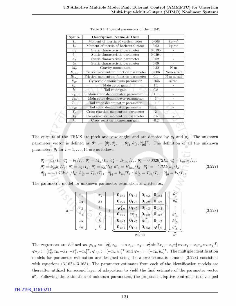
3.3 Adaptive Multiple Model Fault Tolerant Control (AMMFTC) for UncertainMulti-Input-Multi-Output (MIMO) Nonlinear Systems
Table 3.4: Physical parameters of the TRMS
Symb. Description, Value & Unit
Iv Moment of inertia of vertical rotor 0.068 kg-m2
Ih Moment of inertia of horizontal rotor 0.02 kg-m2
a1 Static characteristic parameter 0.0135 -
b1 Static characteristic parameter 0.0294 -
a2 Static characteristic parameter 0.02 -
b2 Static characteristic parameter 0.09 -
Mg Gravity momentum 0.32 N-m
B1αv Friction momentum function parameter 0.006 N-m-s/rad
B1αhFriction momentum function parameter 0.1 N-m-s/rad
kgy Gyroscopic momentum parameter .0155 s/rad
km Main rotor gain 1.1 -
kt Tail rotor gain 0.8 -
T11 Main rotor denominator parameter 1.1 -
T10 Main rotor denominator parameter 1 -
T21 Tail rotor denominator parameter 1 -
T20 Tail rotor denominator parameter 1 -
Tp Cross reaction momentum parameter 2 -
T0 Cross reaction momentum parameter 3.5 -
kc Cross reaction momentum gain -0.2 -
The outputs of the TRMS are pitch and yaw angles and are denoted by y1 and y2. The unknown
parameter vector is defined as θ∗ := [θ∗1, θ∗2, . . . , θ
∗14, θ
∗15, θ
∗16]
T . The definition of all the unknown
parameters θi for i = 1, . . . , 14 are as follows.
θ∗1 = a1/Iv ; θ∗2 = b1/Iv; θ
∗3 = Mg/Iv; θ
∗4 = B1αv/Iv; θ
∗5 = 0.0326/2Iv ; θ
∗6 = kgya1/Iv;
θ∗7 = kgyb1/Iv; θ∗8 = a2/Ih; θ
∗9 = b2/Ih; θ
∗10 = B1αh
/Ih; θ∗11 = −1.75kca1/Ih;
θ∗12 = −1.75kcb1/Ih; θ∗13 = T10/T11; θ
∗14 = km/T11; θ
∗15 = T20/T21; θ
∗16 = kt/T21
(3.227)
The parametric model for unknown parameter estimation is written as,
x =
x1
x3
x2
x4
x5
x6
=
x2
x4
0
0
0
0
+
01×7 01×5 01×2 01×2
01×7 01×5 01×2 01×2
ϕT1,2 01×5 01×2 01×2
01×7 ϕT2,2 01×2 01×2
01×7 01×5 ϕT1,3 01×2
01×7 01×5 01×2 ϕT2,3
︸ ︷︷ ︸Φ(x,u)
θ∗1θ∗2...
θ∗14θ∗15θ∗16
︸ ︷︷ ︸θ∗
. (3.228)
The regressors are defined as ϕ1,2 := [x25, x5,− sinx1,−x2,−x2
4 sin 2x2,−x4x25 cos x1,−x4x5 cosx1]
T ,
ϕ2,2 := [x26, x6,−x4,−x2
5,−x5]T , ϕ1,3 := [−x5, uv]
T and ϕ2,3 := [−x6, uh]T . The multiple identification
models for parameter estimation are designed using the above estimation model (3.228) consistent
with equations (3.162)-(3.163). The parameter estimates from each of the identification models are
thereafter utilized for second layer of adaptation to yield the final estimate of the parameter vector
θ∗. Following the estimation of unknown parameters, the proposed adaptive controller is developed
121
TH-2198_11610211

3. Adaptive Multiple Model Fault Tolerant Control (AMMFTC) of Nonlinear UncertainSystems with Actuator Failures
following the backstepping methodology detailed in Section 3.3.2.1.
For experimental implementation of the proposed adaptive controller using multiple models, all the
states of the system should be available. However, among the six states in the state vector x(t),
only x1 (pitch angle) and x3 (yaw angle) are available for measurement. Therefore, an Extended
Kalman Filter (EKF, Kalman-Bucy filter) [124] is used to estimate the remaining states of the nonlinear
system. The detailed design of the EKF is provided in Appendix A.3. The initial conditions of the
system are x(0) = [0, 0, 0, 0, 0, 0]T . Similarly the EKF states and the states of the identification
models are also initialized at zero. Since the number of unknown parameters is 16, the number of
identification models required to satisfy the conditions of proposed design N=17. The relative degree
of the pitch and yaw subsystems are found to be ℘1 = ℘2 = 3 and hence the controller gains are
selected as c1 = [c1,i3i=1]=[15, 2.5, 2.5] and c2 = [c2,i3
i=1]=[10, 2.5, 2]. The damping gains are chosen
asc1,2 = c2,2 = g1,3 = g2,3 = 0.5. The gain matrices of the adaptive identification models are considered
as Aµ0 = [diag−14,−14,−16,−16,−14,−14] for µ = 1, 17 and γ = 2. The adaptive rate parameter
Γµ is chosen as Γµ = 20I16. The adaptive weight parameters wµ for second layer of adaptation
are initialized at w(0) = 117117×1. The control input voltages uh and uv are maintained within their
allowable range of [−2.5, 2.5]V. The reference trajectories yr,1 and yr,2 to be tracked by the outputs y1 =
θv and y2 = θh are the outputs of the reference system Gr(s) =
[diag
0.2
9s2 + 10s + 4,
0.2
9s2 + 10s + 4
]
with yd,1 and yd,2 as the inputs. In the following, the system is subjected two scenarios of step signal
and sinusoidal signal tracking to illustrate the tracking capability of the proposed multiple model
adaptive controller featuring transient performance improvement without significantly increasing the
control energy.
• Scenario I : This scenario demonstrates sine command tracking performance of the proposed
adaptive controller. The inputs to the reference system are chosen as yd,1 = 6 + 4 sin(0.05πt)
and yd,2 = 12 cos(0.05πt). Figure 3.18(b)-(c) shows satisfactory output tracking capability for
both pitch and yaw angles θv = x1 and θh = x3 with the proposed control scheme. From
a closer glance at the tracking performance in Figure 3.18(a), it is observed that the pitch
and yaw error signals exhibit no substantial transients and ultimately oscillates in the range
[−0.02, 0.04] and [−0.02, 0.15] at steady state. The maximum percentage of steady state error in
tracking with reference to the peak value of yr,1 and yr,2 corresponding to each of the outputs
y1 and y2 is approximately found to be 6% and 14%, respectively. The control input voltages
uv and uh are bounded within their limits. To further our insights on the prolific features
of the proposed adaptive control methodology, a tabulation of output and input performances
are provided in Table 3.5. A low value of root mean square error (RMSE) and integral of
absolute error (IAE) essentially hints at a good steady state performance. Whereas, the integral
of time absolute error (ITAE) metric is meant to measure the transient performance and is
desired be of a small magnitude for fast tracking and stabilization. The inferences drawn from
quantifications of the output tracking performance in Table 3.5 are fairly consistent with our
claims of acceptable transient and steady state performance. The input performance is measured
using control energy(CE) defined as the second norm of the control signal and total variation
122
TH-2198_11610211

3.3 Adaptive Multiple Model Fault Tolerant Control (AMMFTC) for UncertainMulti-Input-Multi-Output (MIMO) Nonlinear Systems
Table 3.5: Tabulation of input and output performances quantified using suitable performance measures
Reference
Signal
Output Performance Input Performance
RMSE IAE ITAE Mp Mu CE TV
Sine trackingθv 0.027 2.364 117.42 - - uv 298.93 217.72
θh 0.062 5.389 276.63 - - uh 164.11 809.38
Step trackingθv 0.011 1.023 20.56 19% 14% uv 288.96 59.40
θh 0.032 3.336 84.08 - - uh 86.15 25.95
(TV) [113] which indicates how frequent the control is used. A small value of TV for a control
scheme is beneficial for practical applications as mentioned in Remark 3.5. The CE and TV
of the control inputs uv and uh corresponding to the proposed controller indicate a fairly good
input performance without excessive chattering. Nevertheless, on a critical assessment of the
error performances, the reader may find the steady state error bounds on a slightly higher side.
However, it is to be mentioned that the performance of the TRMS under the action of the
proposed controller is indeed appreciable given the fact that real time experiments on the TRMS
are subjected to noise, air gust, voltage fluctuations and other unforeseen external disturbances.
• Scenario II : In this case, we study the performance of the proposed control methodology under
step command tracking. Considering the same reference system Gr(s) driven by inputs yd,1 =
4U(t) + 4U(t− 25) − 4U(t − 75) and yd,2 = 6U(t), its outputs yr,1 and yr,2 serve as the desired
trajectories for system output tracking. Here, U(t) is defined as the unit step input. From the
results in Figure 3.19, it is evident that the proposed control scheme is capable of rendering
a good tracking performance for step reference inputs with minimum chattering in the control
input voltages. Further, the control inputs reside within their permissible ranges while realizing
the desired control objective. The pitch tracking error show some transient behaviour with an
overshoot of 19% and an undershoot of 14% with reference to yr,1 = 0.2 while the yaw tracking
error exhibits no peaks beyond yr,2 = 0.3. The maximum steady state error is approximately
calculated to be 5% for θv and 9% for θh. Tabulation of calculated ITAE, IAE, and RMSE values
under step tracking in Table 3.5 reveals a satisfactory and appreciable output performance.
Further, the TV and CE values in Table 3.5 are reasonably low, indicating a promising input
performance. The effect of cross-coupling The yaw tracking performance can be however further
improved using an integral action in the proposed controller. Taking into consideration several
issues in real time implementation as mentioned in the preceding scenario, the performance of
the proposed adaptive control system is certainly acceptable. The authors do believe that the
obtained results are indeed appreciable and encouraging.
Remark 3.5. At this juncture, it should be remarked upon that the proposed adaptive control method-
ology contributes in two directions. Firstly, it offers a control solution to the tracking problem in
unknown nonlinear uncertain systems featuring an improved output transient performance. Secondly,
123
TH-2198_11610211

3. Adaptive Multiple Model Fault Tolerant Control (AMMFTC) of Nonlinear UncertainSystems with Actuator Failures
Time [s]0 10 20 30 40 50 60 70 80 90 100O
utpu
t tra
ckin
g er
ror
(rad
)
-0.2
-0.1
0
0.1
0.2x1 − yr,1 x3 − yr,2
(a)
0 10 20 30 40 50 60 70 80 90 1000
0.2
0.4
0.6
0.8
Time [s]
Pitc
h an
gle
(rad
)
(b)
0 10 20 30 40 50 60 70 80 90 100
−0.5
0
0.5
1
Time [s]
Yaw
ang
le (
rad)
(c)
Time [s]0 10 20 30 40 50 60 70 80 90 100C
ontr
ol in
put v
olta
ges
(V)
-2
-1
0
1
2
3
Main rotor voltage uv Tail rotor voltage uh
(d)
Figure 3.18: (a) pitch and yaw angle tracking error (rad) ; (b) pitch angle θv = x1(rad); (c) yaw angle θh = x3(rad); (d)control input voltages uv and uh (V).
124
TH-2198_11610211

3.3 Adaptive Multiple Model Fault Tolerant Control (AMMFTC) for UncertainMulti-Input-Multi-Output (MIMO) Nonlinear Systems
Time [s]0 10 20 30 40 50 60 70 80 90 100
Tra
ckin
g er
ror
(rad
)-0.1
-0.05
0
0.05
0.1
x1 − yr,1 x3 − yr,2
(a)
Time [s]0 10 20 30 40 50 60 70 80 90 100
Pitch
angle
θv=
x1(rad)
0
0.1
0.2
0.3
0.4
0.5
yr,1 x1
(b)
Time [s]0 10 20 30 40 50 60 70 80 90 100
Yaw
angle
θh=
x3(rad)
0
0.1
0.2
0.3
0.4
0.5
0.6
yr,2 x3
(c)
Time [s]0 10 20 30 40 50 60 70 80 90 100
ControlInputs
(V)
-2
0
2
4
Main rotor voltage uv Tail rotor voltage uh
(d)
Figure 3.19: (a) pitch and yaw angle tracking error (rad) ; (b) pitch angle θv = x1(rad); (c) yaw angle θh = x3(rad); (d)control input voltages uv and uh (V).
125
TH-2198_11610211

3. Adaptive Multiple Model Fault Tolerant Control (AMMFTC) of Nonlinear UncertainSystems with Actuator Failures
the obtained solution can be further utilized to solve FTC problems using adaptive control and cater to
the requirements of enhanced post failure transient performance without substantial increase in control
usage. Adhering to the aim of FTC, the performance of the proposed AMMFTC scheme was demon-
strated for control of MIMO nonlinear uncertain systems affected by abrupt actuator faults through
extensive simulations in Section 3.3.4. Further, the proposed control methodology was experimentally
implemented to control the attitude of a twin rotor MIMO system (TRMS). Given the fact, an abrupt
decrease in thrust forces generated by the rotors would emulate the occurrence of actuator faults, it is
certainly not possible to practically realize actuator faults in such an experimental set-up. It should
be clearly understood that scaling the parameters θ∗14 and θ∗16 associated with the control voltages uv
and uh do not model partial loss of effectiveness of actuators. Hence, the experiments were conducted
without considering the occurrence of actuator faults. Nevertheless, the parameters of the TRMS were
assumed to be unknown and estimated using the adaptation algorithm proposed in this chapter. The
results obtained are promising. Any loss of actuation effectiveness will lead to change in the values of
constant unknown parameters associated with Lm and Lt. Therefore, under this scenario, if a satisfac-
tory transient and steady state performance is achieved at start up, it is reasonable to assume that the
proposed adaptive controller would exhibit similar attributes at post fault scenarios.
3.4 Summary
In this chapter, a new actuator failure compensation strategy was presented for nonlinear uncertain
systems. The design methodology followed a multiple model adaptive backstepping procedure without
switching and tuning. The proposed method exhibits a simpler structure compared to [54], [24] and
[100] in the sense that a single controller is utilized in the design of failure compensation in the event of
unknown actuator LOE, LIP and float free failures. The proposed controller was developed in a manner
so as to be able to compensate infinite actuator failures. Unlike existing literature on adaptive FTC
in regards to intermittent actuator failures, explicit output error bounds in terms of L∞ and L2 signal
measures are derived by formulating the closed loop dynamics as a random impulsive hybrid system.
Besides, the improvement of output transient performance using the proposed FTC strategy is proved
theoretically through an appropriate quantification. Finally, the proposed controller fed with parameter
estimation from a minimum number of estimation models adds up to the computational simplicity of
the method presented. Thereafter, the AMMFTC algorithm is extended to control of MIMO nonlinear
systems with actuator failures. Similar design attributes were observed and the controller was able
to suppress overshoots due to actuator failures as well as those due to cross coupling effects. In
addition, the control input performance was also observed to be acceptable. Thus, the proposed
control algorithm conforms with the desired FTC design requirements and qualifies to be a suitable
scheme for practical applications. It is expected to achieve promising results in large scale MIMO
systems as well. Simulation results illustrate the effectiveness of the proposed FTC method in the case
of actuator faults/failures for both single input multi output and MIMO nonlinear uncertain systems.
126
TH-2198_11610211

4Finite Time Adaptation based
Compensation (FTAC) of Actuator
Failures in Nonlinear Uncertain Systems
Contents
4.1 Introduction . . . . . . . . . . . . . . . . . . . . . . . . . . . . . . . . . . . . . 128
4.2 Finite Time Adaptation based Compensation (FTAC) of Infinite Actua-
tor Failures . . . . . . . . . . . . . . . . . . . . . . . . . . . . . . . . . . . . . . 132
4.3 Finite Time Adaptation based Compensation (FTAC) of Actuator Fail-
ures in Multi-Input-Multi-Output (MIMO) Nonlinear Uncertain Systems 165
4.4 Summary . . . . . . . . . . . . . . . . . . . . . . . . . . . . . . . . . . . . . . . 187
127
TH-2198_11610211

4. Finite Time Adaptation based Compensation (FTAC) of Actuator Failures in NonlinearUncertain Systems
4.1 Introduction
Pertinent to nonlinear systems, the adaptive multiple model based fault estimator (FE) integrated
FTC algorithm proposed in Chapter 3, is certainly a promising attempt to overcome the design limi-
tations encountered in direct adaptive FTC and existing ARFTC methods. Such an algorithm enjoys
the merits of (1) modularity between the controller-estimator pair; (2) enhanced output transient per-
formance without decreased stability margins at start up and post-failure; (3) faithful compensation
of infinite actuator failures; (4) globally asymptotically stable fault tolerant output tracking; and (5)
increased design freedom. Despite exhibiting a plethora of prolific features, the computational com-
plexity is only alleviated to an extent on account of a significant decrease in the number of identifiers.
Although the multiple model estimator with two layer of adaptation in Chapter 3, exhibits compar-
atively faster convergence, it can only guarantee boundedness of parameter estimates. Moreover, the
parameter estimates converge to their true values if and only if the restrictive persistence of excitation
(PE) condition is met by the regressor signals. Further, the parameter convergence time cannot be
exactly characterized. It is always a good practice to explore new rewarding adaptive control methods
for FTC applications which offer excellent robust performance and at the same time are computation-
ally appealing. Along similar lines, the search for algorithms to arrive at an ideal adaptive solution,
is indeed akin to the infinite quest for the “Holy Grail” in active FTC design for nonlinear uncertain
systems. Within the proposed active FTC architecture, the time available for fault estimation and
subsequent recovery plays a crucial role in deciding the existence of stable adaptive solutions. Con-
sidering practical situations such as in mission critical systems, where the time window in which the
faulty system is stabilizable is very short [8, 94], this time is strictly small. As a matter of fact, if the
actuator fault/failure is not accommodated within a specific finite time, the inputs and outputs will
encroach their safety limits and eventually lead to mission failures, which is undesirable.
In view of the design objectives of fast failure recovery, transient improvement, acceptable control
usage (within predefined physical limits) and computational simplicity; the strong controller developed
in Chapter 3, when augmented with a finite time parameter estimator would be a promising choice
for FTC applications, where time is a critical parameter. Introduction of finite time stable parameter
estimators into the design allows for an upper bound on the time required for fault estimation. Thus,
such a modification will add to the design freedom of the FE/FTC architecture proposed in Chapter 3.
In consequence, the damping parameters can be tuned accordingly to maintain the design modularity
and obtain a control input within its allowable limits. It is well known that output performance in
an indirect adaptive control approach is directly related to the estimation performance. Hence, the
estimator featuring finite time convergence will ensure accurate estimation of failure induced parameters
and contribute to the improvement of output transient performance. Besides, stability margins remain
unaffected and are certainly enhanced, if not decreased. Motivated by the above insights and reasonable
arguments, a finite time adaptation based control (FTAC) is designed in this chapter for application
to the development of failure resilient nonlinear control systems. The control design herein utilizes
an ISS backstepping controller augmented with a novel finite time parameter estimator. The design
features of the proposed finite time parameter estimator will be discussed in the sequel. To the best of
authors’ knowledge, there are still no results available in FTC literature which propose an integrated
128
TH-2198_11610211

4.1 Introduction
FE/FTC design framework featuring finite time fault/failure estimation in linearly parameterizable
nonlinear uncertain systems. Further, an FTAC solution to the problem of compensating possible
infinite actuator failures followed by a rigorous analysis is also not attempted so far. Therefore,
the FTAC method developed in this chapter is also extended to adaptive compensation design for
intermittent actuator failures followed by rigorous analysis of signal convergence properties. The
results obtained are indeed encouraging. Compared to AMMFTC method, the proposed technique
obviates the usage of multiple identification models and hence the computational burden is expected
to be further reduced. In summary, the proposed control method exhibits all the desirable attributes
of an ambitious FTC strategy.
Apart from its promising contributions to FTC literature, the proposed algorithm is also anticipated
to be a value addition to existing control schemes with finite time parameter estimation. Such a
claim certainly requires well substantiated and strong arguments to endorse the proposed controller
and to arrive at conclusions justifying its design uniqueness. In what follows, we discuss the FTAC
methodology in brief and its contributions compared to relevant existing results on adaptive control
with finite time adaptation.
With reference to the FTAC algorithm developed in this chapter, parameter convergence is justi-
fied to be a fundamental design element which decides performance improvement and also contributes
to the enhancement of robust stability of the closed loop adaptive system. Recent years have wit-
nessed an influx of generalized second order sliding mode ideas to solve the problem of finite time
parameter identification in nonlinear systems as a part of observer design [125–128]. The resulting
robust parameter adaptation algorithms claim exact estimation of unknown parameters in finite time.
However, the following drawbacks restrict their applicability to general nonlinear systems with linearly
parameterized uncertainties.
• Finite time parameter estimation is possible only for linear stable systems and Lipschitz nonlinear
systems.
• Apart from assuming that the system states are accessible for measurement, these observer based
parameter estimation approaches also require the measurement or computation of the velocity
state vector.
• The invertibility of the regressor matrix has to be continuously checked online and the matrix
inverse has to be computed for parameter estimation.
• Inapplicable for unstable systems regardless of their dynamics being linear or nonlinear.
In addition to the above-mentioned shortcomings, it is also observed that integration of these parameter
estimators driven by state predictor/observer error, with a controller fails to yield parameter conver-
gence to their true values. As a result, output performance is adversely affected. The disadvantages
of observer based adaptive parameter estimation approaches have immensely motivated the design
of parameter prediction error dependent estimators to improve estimator convergence characteristics.
Certainly, to the best of our knowledge, finite time parameter estimation in adaptive control of non-
linear systems has been pioneered by Adetola and Guay in [129]. The adaptation algorithm proposed
129
TH-2198_11610211

4. Finite Time Adaptation based Compensation (FTAC) of Actuator Failures in NonlinearUncertain Systems
in [129], ensures exact estimation of unknown parameters after a finite time whose magnitude is depen-
dent on the observed excitation of the filtered regressor signals. The estimation performance superiority
in comparison to standard parameter estimators has been well demonstrated therein. In [130], an in-
tegrated finite time adaptive estimation based controller is designed to improve output performance
and achieve asymptotic stability of the tracking error. In [130], the adaptation algorithm resorts to the
finite time parameter estimation algorithm in [129] and uses both the tracking error and parameter
prediction error for performance enhancement. In [129], the PE condition on the regressor signals
transforms to online checking for non-singularity of the time integrated function of filtered regressor
matrix for each sampling interval. This is indeed obligatory for the algorithm proposed in [129] in the
sense that the estimation method explicitly computes the inverse of the foregoing integral of interest
on the run to arrive at the parameter estimate. From a computational perspective, it is natural to
conclude that such continuous online check for existence and subsequent computation of inverses lead
to increased computational complexity with increase in the dimension of unknown parameter vector.
Thus, to make the design amenable to practical computational constraints, the authors suggested the
invertibility check from t = 0 to a time tc after which the integral of the filtered regressor function
is positive definite. The parameter adaptation is stopped after time tc. However, actuator failures
are unanticipated both in time and magnitude. Therefore, in regards to FTC design, such a remedial
measure to lend computational simplicity is practically infeasible. Besides, no closed form expression
has been provided in [129] to determine the convergence time of the parameter estimation error. Adap-
tive parameter estimators utilizing ideas from sliding mode control (SMC) have also been proposed
recently [131] to guarantee finite time convergence. The parameter estimation obtained from an SMC
estimator contains high frequency components and is not smooth. As a consequence, the input perfor-
mance is compromised whenever sliding mode parameter estimation is incorporated into an integrated
estimation based control design.
A novel finite time adaptive parameter estimator driven by parameter prediction error, is proposed
in this chapter. Apart from assuring finite time parameter estimation, the proposed algorithm elim-
inates all the limitations of the above cited literature. From the view point of finite time parameter
estimation based adaptive control, the proposed method builds upon the work of Adetola and Guay
in [129]. The proposed estimator design initiates by introducing several stable filters to obtain the
filtered versions of the state vector and regressor matrix. On account of a passivity based low pass fil-
tering of the regressor matrix, stability of estimation error and inherent signals are ensured irrespective
of the boundedness of the regressor matrix. Thereafter, two additional low pass filters with their inputs
being functions of filtered regressor matrix and state vector are introduced to yield two auxiliary design
variables. The parameter estimation error is then defined using these auxiliary variables. Finally, the
proposed adaptive law is developed utilizing concepts from second order sliding mode control [132]. The
parameter update law does not require any knowledge of the time derivative of parameter prediction
error. The estimation is continuous and smooth without chattering. Unlike [129], the usage of low pass
filters in arriving at the expression for parameter error circumvents the online check for existence and
computation of inverse for the filtered regressor matrix. The integral laws proposed in [129] to relax
PE condition, may result in integrator wind up and hence unboundedness of adaptation may occur.
130
TH-2198_11610211

4.1 Introduction
This drawback is very serious, especially when practical applications are considered and is eliminated
by the proposed adaptation algorithm. Furthermore, as an added advantage, robustness of parameter
estimation to external disturbances is also guaranteed. Parameter convergence to their true values
is guaranteed, using the proposed estimator without the need of the PE condition. However, a more
relaxed initial excitation (IE) condition [133] needs to be satisfied to achieve faithful parameter estima-
tion. Exponential stability of tracking error is guaranteed provided the IE condition is fulfilled. The
parameter prediction error and its time derivative using the proposed adaptation technique converge
to zero at steady state. Under the integrated estimator based FTC scheme proposed herein, such an
attribute indeed adds to further improvement of input performance and accuracy of output tracking
at steady state.
As the third contribution in this chapter, the proposed FTAC method is also applied to solve the
adaptive FTC design problem in nonlinear coupled MIMO systems affected by large unknown paramet-
ric uncertainties and actuator failures/faults. Although not straightforward, the design methodology
is utilized to develop the proposed FE/FTC control architecture. Similar to the results obtained for
MISO systems, convergence and stability properties of the output error, estimation error and other
intermediate signals do not change when the FE/FTC scheme with finite time adaptation is applied
to control of MIMO nonlinear systems. Further, to investigate its suitability for practical applications,
the proposed FTAC algorithm is utilized to design an adaptive attitude controller for the laboratory
prototype of a 2-DOF helicopter (Twin Rotor MIMO system, TRMS) assuming that its parameters
are totally unknown. The results obtained are satisfactory which prove that performance efficacy and
robustness of the proposed FTAC strategy.
Rest of the chapter is organized as follows: Section 4.2 presents the design of finite time adaptation
based controller (FTAC) for nonlinear uncertain systems to compensate finite and infinite actuator
failures. Prior to the description of the design methodology, some preliminary definitions are stated
in subsection 4.2.1. Further, the problem formulation and design assumptions appear in subsection
4.2.2. Thereafter, the proposed controller and finite time estimator are discussed in subsection 4.2.3.
A rigorous closed loop stability analysis is provided in subsection 4.2.4. A detailed simulation study is
conducted in subsection 4.2.5. Section 4.3 deals with the extension of FTAC strategy coupled MIMO
nonlinear systems with unknown parameters and actuator failures. Subsection 4.3.1 formulates the
FTC design problem along with the necessary assumptions for MIMO nonlinear systems while sub-
section 4.3.2 describes the FTAC design procedure. Subsection 4.3.3 presents the closed-loop stability
analysis of the proposed control system. In subsection 4.3.4, simulation studies are described and the
results obtained are illustrated. Subsection 4.3.5 presents the experimental results obtained by apply-
ing the proposed FTAC methodology to attitude control of a twin rotor MIMO system. Finally, the
summary of Chapter 4 is drawn in Section 4.4.
131
TH-2198_11610211

4. Finite Time Adaptation based Compensation (FTAC) of Actuator Failures in NonlinearUncertain Systems
4.2 Finite Time Adaptation based Compensation (FTAC) of Infinite
Actuator Failures
4.2.1 Some Preliminary Definitions
Definition 4.1. Let us consider a signal x(t) ∈ Rn and consider the set,
S1(ν) =
x : [0,∞) 7→ R
n∣∣∣t+T∫
t
|x(s)|ds ≤ λ0νT + λ1, ∀t, T > 0
for a given constant ν ≥ 0 with λ0, λ1 > 0 are finite constants. The signal x(t) is said to be ν−small
in the absolute sense (a.b.s) if x(t) ∈ S1(ν).
Definition 4.2. Let us consider a signal x(t) ∈ Rn and consider the set,
S2(ν) =
x : [0,∞) 7→ R
n∣∣∣t+T∫
t
xT (s)x(s)ds ≤ (λ0ν2 + λ1ν)T + λ2, ∀t, T > 0
for a given constant ν ≥ 0 with λ0, λ1, λ2 > 0 are finite constants. The signal x(t) is said to be
ν−small in the mean square sense (m.s.s) if x(t) ∈ S2(ν).
Definition 4.3. A bounded signal x(t) ∈ Rn is persistently exciting (PE) for t ∈ [0, ∞) provided
∃T > 0 and λ > 0 such that the following condition holds ( [133], [134]),
t+T∫
t
x(s)xT (s)ds ≥ λIn, ∀t ≥ 0
where In denotes an identity matrix of order n.
Definition 4.4. A bounded signal x(t) ∈ Rn is exciting over the finite time interval [t0, t0 + T ) with
T > 0 and t0 ≥ 0, provided ∃ λ > 0 such that the following condition holds ( [133]),
t0+T∫
t0
x(s)xT (s)ds ≥ λIn
where In denotes an identity matrix of order n.
Theorem 4.1. Let us consider a continuously differentiable function V : D × [0,∞) → R+, finite
positive numbers Γ > 0, µ ∈ (0, 1), and a neighborhood N ⊂ D of the origin such that V is positive
definite over N and V + ΓV µ is negative semi-definite over N where V (x) ,∂V (x)∂x f(x). Then the
origin is a finite-time-stable equilibrium of the dynamics x = f(x). Further, if Ts defines the settling
time function, then Ts(x) ≤ 1Γ(1−µ)V (x)1−µ ∀x in the open neighborhood of the origin [106].
132
TH-2198_11610211

4.2 Finite Time Adaptation based Compensation (FTAC) of Infinite Actuator Failures
4.2.2 Problem Formulation
On similar lines as in 3.2, let us consider a class of nonlinear uncertain systems transformable to a
parametric strict feedback form as follows.
xi = xi+1 + fi(xi)Tκ∗, i = 1, ℘− 1 (4.1)
x℘ = f0(x, η) + f℘(x, η)T κ∗ +
m∑
j=1
bjβj(x, η)uj (4.2)
y = x1 (4.3)
η =Λ0(x, η) +
p∑
i=1
κ∗iΛi(x, η) (4.4)
where xi(t) for i = 1, ℘ represent the states of the dynamical system (4.1)-(4.2) and ℘ defines the rel-
ative degree of the plant with reference to its output. The notation xi(t) is meant to denote a i−tuple
state vector and x(t) = [x1, . . . , x℘]T ∈ R℘ defines the full state vector. The system output is given
by y defined by a state or a smooth function of the states. The functions fi(·, ·) : R℘ × R
n−℘ → Rp
for i = 1, ℘ are assumed to be vectors of known smooth linear/nonlinear functions. Further, f0(·, ·) is
also a known nonlinear function which is infinitely continuously differentiable. The actuation functions
βj(·, ·) : R℘ × R
n−℘ → R ∈ C∞ for j = 1,m are known and may not be necessarily linear. The factors
bj for j = 1,m define the unknown control coefficients. Further, the uncontrollable dynamics of the
system is described by η. The unknown vector of system parametric uncertainty is denoted by κ∗ ∈ Rp
where its elements are unknown constants or may be time varying.
Prior to the formulation of the FTC problem, the input-output characteristics of the actuators encom-
passing their healthy, faulty and failure states of operation are to be defined. Given that uHj defines the
input and Kj,h describing the state of health of the j−th actuator during time t ∈ [toj,h, tej,h) ⊂ [0, ∞),
the actuator failure model is described as,
uj(t) =
Kj,huHj + uFj,h, t ∈ [toj,h, t
ej,h)
uHj , t ∈ [tej,h, toj,h+1)
(4.5)
The suffix ‘o’ and ‘e’ is used to denote the onset and end of a particular actuator failure pattern for
the time interval t ∈ [th, th+1). The notation uFj,h is used to represent the magnitude at which the
j − th actuator is jammed after it fails completely. It has been discussed in Section 3.2 that the above
modeling encompasses three forms of actuator faults and failures, namely; loss of effectiveness(LOE),
lock-in-place(LIP) and float failure.
Now assuming that actuators in the system may undergo abrupt and sudden faults/failures, the control
design objectives are as follows,
• Guaranteeing stability of the closed-loop system under occurrence of the considered types of
actuator failures unknown in time pattern and magnitude for all time t ∈ [0, ∞).
• Fast, accurate and finite time estimation of unknown system and failure induced parameters
leading to an improved output transient and steady state performance.
133
TH-2198_11610211

4. Finite Time Adaptation based Compensation (FTAC) of Actuator Failures in NonlinearUncertain Systems
• Output tracking is robust to unknown system and actuator failure parameters assumed to vary
intermittently across all time t ∈ [0, ∞). Given that the system undergoes possible infinite
parameter jumps not necessarily known, the output tracking error y(t) − yr(t) is ensured to be
stable and ν−small in the absolute sense (a. b. s.), i.e., z1(t) := (y(t) − yr(t)) ∈ S1(ν).
• In case the total number of actuator failures and system parameter jumps are finite, asymptotic
convergence of output tracking error to the origin is ensured, that means, limt→∞
z1(t) = 0.
4.2.2.1 Design Assumptions
The same set of assumptions as in Section 3.2 are invoked prior to controller design to meet the
aforementioned objectives. The assumptions are not repeated in detail here for the sake of brevity in
presentation. In summary, the fault tolerant control design assumes that the system is controllable
with respect to (m− 1) actuator failures adding to the non-singularity of the resulting actuation func-
tion, that is, βj(x, η) 6= 0. This condition guarantees the existence of an adaptive control solution to
the concerned actuator FTC problem. The signs of the actuation coefficients sign(bj) for j = 1,m is
known. The internal dynamics (4.4) of order (n − ℘) is input-to-state-stable(ISS) with respect to the
controllable states (x(t)) as its input. The reference trajectory yr(t) and their successive time deriva-
tives until ℘−th order are continuous, bounded and belong to a compact set. Besides, the unknown
failure and system parameters satisfy Assumption 3.5 meaning that 0 < bj ≤ |bj | ≤ bj, |uFj,h| < u
and 0 < Kj ≤ Kj ≤ 1 and bj , bj , umax and Kj for j = 1,m are known finite positive constants.
The unknown parameter vector κ∗ belongs to a known convex compact set, i.e., κ∗ ∈ Sκ∗ ⊂ Rp. The
set Sκ∗ is the convex compact set where the parameter vector κ∗ ∈ Rp resides and ∀κ1, κ2 ∈ Sκ∗ , the
relation ‖κ1 − κ2‖ ≤ κmax holds.
4.2.3 Fault Tolerant Control Design with Finite Time Adaptation
Actuator redundancy is indispensable in achieving failure tolerance in any dynamical system.
Hence, considering that the actuators of the nonlinear system (4.1)-(4.4) have similar physical and
operational characteristics, the j−th control input can be designed in parallel as,
uHj(t) =1
βjv(t)sign(bj) (4.6)
where v(t) is designed using a backstepping technique with finite time adaptation to improve the
performance. Let us define the actuator index set as B := j1, . . . , jm and two of its subsets comprising
of failed and healthy actuator indices as BtotF = j1, . . . , jqh and BtotH := B/BtotF , respectively.
The notation qh is used to denote the number of totally failed actuators at a failure time instant t = Th
and varies as 0 ≤ qh ≤ (m − 1) all throughout the interval [Th, Th+1) until the onset of the next
consecutive actuator failure pattern at t = Th+1.
Incorporating the actuator failure model (4.5) and the expression for v(t) (4.6) into the system dynamics
134
TH-2198_11610211

4.2 Finite Time Adaptation based Compensation (FTAC) of Infinite Actuator Failures
(4.1)-(4.2), the unified model with actuator failure parameters can be formulated as,
xi = xi+1 + fi(xi)Tκ∗, i = 1, ℘− 1
x℘ = f0(x, η) + f℘(x, η)Tκ∗ + b∗v + βT u∗ (4.7)
where,
b∗ :=
m∑j=1
|bj|, for Kj,h = 1 and uFj,h = 0∀ j ∈ B
∑j∈BtotH
Kj,h|bj |, for Kj,h ∈ [0, 1) and uFj,h 6= 0 ∀ j ∈ BtotF
(4.8)
u∗ := [0, . . . , 0]T ∈ Rm, for Kj,h = 1 and uFj,h = 0 ∀ j ∈ B (4.9)
u∗ := [bjk uFjk,hqhk=1, 0, . . . , 0]
T ∈ Rm for Kj,h ∈ [0, 1) and uFj,h 6= 0 ∀ j ∈ BtotF (4.10)
Finally, the vector of unknown parameters due to abrupt actuator faults/failures and unknown param-
eters in modeling is defined by θ∗ := [θ∗1 θ∗2 θ
∗3]T = [b∗ κ∗ u∗]T ∈ R
p+m+1. The parameter θ∗1 and θ∗3are actuator fault/failure induced perturbations and hence are time varying with θ∗1,θ
∗3 6= 0 implying
θ∗(t) 6= 0. Nevertheless, θ∗1 and θ∗3 can be considered to be approximately zero if the cardinality of
occurrence of actuator failure is finite and the inter-event time between two successive failure events
is substantially large. Owing to intermittent changes in the failure induced parameters resulting from
changes in the actuator failure pattern for every T ∗ := (Th+1 − Th) > 0, for h ∈ W and t ∈ [0, ∞),
θ∗(t) satisfies the following property [6] stated in Lemma 4.1.
Lemma 4.1. The time derivative of the unknown parameter vector θ∗(t) representing system and
actuator failure induced parametric uncertainties satisfy θ∗(t) ∈ S1(ν), i.e.,
t+T∫
t
‖θ∗(s)‖ds ≤√m+ p+ 1∆†νT +
√m+ p+ 1∆†; ∀t ∈ [t, t+ T ) (4.11)
where ν = 1T ∗ > 0, ∆† = max
m∑j=1
bj − ℓ, 2bju < ∞ and ℓ = min1≤j≤m
Kjbj. The time span T ∗ is the
minimum of all the time intervals between two consecutive changes in the actuator fault/failure pattern
and the constants bj , u > 0 are derived from the design assumptions in Section 4.2.2.
Proof. The proof is provided in Appendix A.4.
Remark 4.1. It is well known that unknown parameters in any dynamical system vary with time. Given
the fact that their variation with time is sufficiently slow, it is an universal assumption to consider them
as constants and that their time derivatives are zero. This assumption is widely cited in the design
and stability analysis of any adaptive or adaptive robust control methodologies in literature. Unlike the
works in literature, since the adaptive control design concerns compensation of time varying actuator
faults and failures, the proposed FTC design does not consider the time derivative of the unknown
135
TH-2198_11610211

4. Finite Time Adaptation based Compensation (FTAC) of Actuator Failures in NonlinearUncertain Systems
parameter vector θ∗(t) to be zero. For the case of finite variations in actuator failure patterns and
system parameters not assumed to be sufficiently close, taking the integral in (A.4.3) from 0 ∼ T and
T ∗ → ∞(ν → 0), we get θ∗(t) ∈ L1[0, T ). Where, [0, T ) denotes the maximal interval of existence of
θ∗(t). This result would be utilized later to prove the asymptotic stability of the tracking error dynamics
in the event of changes in actuator failure patterns with finite cardinality. At this juncture, it is worth
mentioning that in presence of unknown piecewise constant time varying parameters, the property of
θ∗(t) in (A.4.3) and its subsequent usage in the stability analysis, will provide a clear insight to infer
the signal characteristics of the output tracking error z(t) for all t ∈ [0, ∞).
4.2.3.1 Design of Finite Time Parameter Estimator
In this subsection, a new parameter estimator featuring fast and finite time convergence to the
actual parameter is proposed. Some necessary filters are introduced and boundedness properties of
filtered signals and their derivatives are studied a priori. The adaptive law guaranteeing accurate and
finite time parameter estimation is presented thereafter followed by derivation of stability properties
of the estimator.
The estimator design procedure starts with representing the nonlinear dynamical system with failure
parametrization (4.7) as a parametric x−model as given below.
x = f(x) + ΦT (x, v)θ∗ (4.12)
where, f(x) and Φ(x, v) are defined as follows,
f(x) = [x2, x3, . . . , x℘, f0(x, η)]T ∈ R
℘ & ΦT (x, η) =
0 f1(x1)T 01×m
0 f2(x2)T 01×m
......
...
v fp(x, η)T βT
∈ R
℘×p+m+1.
At this point, let us introduce the following filters.
ΩT = A(x, t)ΩT + ΦT (x, v); Ω ∈ R(m+p+1)×℘ (4.13)
Ω0 = A(x, t)(Ω0 + x) − f(x); Ω0 ∈ R℘ (4.14)
where, A(x, t) = A0 − γΦ(x, v)TΦ(x, v)P . Further, A0 is a constant Hurwitz matrix with a positive
definite matrix P = P T > 0 as the solution to the equality AT0 P +PA0 +Q = 0 with a chosen Q > 0.
Additionally, we define another two filters with filtered variables R(t) and S(t) as,
R(t) = −K R(t) + ΩΩT ; R(0) = 0, R(t) ∈ R(m+p+1)×(m+p+1) (4.15)
S(t) = −K S(t) + Ω(Ω0 + x); S(0) = 0, S(t) ∈ Rm+p+1 (4.16)
where K > 0 is another design scalar. Now, we have the following lemmas which are essential prior
to development of stability properties of the proposed controller.
136
TH-2198_11610211

4.2 Finite Time Adaptation based Compensation (FTAC) of Infinite Actuator Failures
Lemma 4.2. Let the maximal interval of existence of solutions of filter dynamics (4.13) be [0, T ).
Then filtered signal Ω(t) is bounded irrespective of the boundedness of the regressor matrix Φ, i.e.,
Ω(t) ∈ L∞[0, T ). The L∞ bound is given by,
‖Ω‖∞ ≤ √℘
(√λ(P )
λ(P )‖Ω(0)‖F +
√m+ p+ 1
2γλ(Q)
)
where ‖ · ‖F denotes the Frobenius norm of the argument matrix.
Proof.
The proof follows a similar procedure as outlined in Section 4 of Chapter 6 in [69]. The boundedness
of Ω(t) is derived as follows.
d
dt(ΩPΩT ) = Ω(AT0 P + PA0)Ω
T − 2γΩPΦTΦPΩT + ΩPΦT + ΦPΩT
= −ΩQΩT − 2γ
[ΩPΦTΦPΩT − 2
1
2γΦPΩT +
1
4γ2Im+p+1
]+
1
2γIm+p+1
= −ΩQΩT − 2γ
[ΦPΩT − 1
2γIm+p+1
]T[ΦPΩT − 1
2γIm+p+1
]+
1
2γIm+p+1 (4.17)
Now taking trace(·) operator on both sides of the equality (4.17) yields,
d
dttrace(ΩPΩT ) ≤ −λ(Q)‖Ω‖2
F − 2γ‖ΦPΩT − 1
2γIm+p+1‖2
F +1
2γtrace(Im+p+1) (4.18)
≤ −λ(Q)‖Ω‖2F +
m+ p+ 1
2γ(4.19)
Now using the fact that λ(P )‖Ω‖2F
≤ trace(ΩPΩT ) and the property of norm inequalities (Page
47, [122]) ‖Ω‖∞ ≤ √℘‖Ω‖2 along with ‖Ω‖2 ≤ ‖Ω‖F , the following is obtained.
‖Ω‖∞ ≤ √℘
(√λ(P )
λ(P )‖Ω(0)‖F +
√m+ p+ 1
2γλ(Q)
)(4.20)
The proof is complete.
Combining (4.12) and (4.14), let us define an auxiliary variable Y := Ω0 + x such that,
Y = (A0 − γΦ(x, v)TΦ(x, v))Y + Φ(x, v)T θ∗ (4.21)
Before proceeding further, stating the following lemma is necessary.
Lemma 4.3. The filtered regressor matrix R(t) obtained as solution of (4.15) is positive definite if
and only if Φ(x, v) in (4.12) is persistently exciting (PE).
Proof.
From the proof of Lemma 4.2, the presence of the matrix A(x, t) = (A0 − γΦ(x, v)TΦ(x, v)) in (4.13)
yields strongly stable and bounded trajectories of Ω even though the regressor matrix is unbounded.
137
TH-2198_11610211
4. Finite Time Adaptation based Compensation (FTAC) of Actuator Failures in NonlinearUncertain Systems
Hence A(x, t) is inferred to be a stable matrix. Now, in accordance with the statement of the proof, it
is apriori assumed that Φ(x, v) is PE. Since, the filter dynamics (4.13) is stable and minimum phase,
the PE for Ω holds straightaway and hencet+T∫t
Ω(s)ΩT (s)ds ≥t+T∫t
min√λ(Ω(s)ΩT (s))Im+p+1ds ≥
Im+p+1 [133]. Here λ(·) denotes the eigen values of its argument and Im+p+1 is the identity matrix
of order (m+ p+ 1). Now the solution R(t) of the additional filter in (4.15) is given by,
R(t) =
t+T∫
t
e−K (T−s)Ω(s)ΩT (s)ds (4.22)
The above equality (4.22) is further reiterated in the form of an inequality as stated below.
R(t) = e−K T
t∫
t−T
eK sΩ(s)ΩT (s)ds ≥ e−K T
t∫
t−T
min√
λ(ΩΩT )Im+p+1 ≥ e−K TIm+p+1 (4.23)
The inequality derived in (4.23) holds for t > T and directs the readers to the conclusion that R(t) ≥λ(R(t))Im+p+1 > e−K TIm+p+1 > 0. Hence, R(t) is positive definite. Therefore, it is concluded that
the PE condition on the regressor matrix Φ(x, v) now translates to ensuring the positive definiteness
of R(t).
Now, defining Y := Y − ΩT θ∗, the derivative of Y is calculated from (4.21) as,
˙Y = (A0 − γΦTΦ)Y + ΦT θ∗ − ((A0 − γΦTΦ)ΩT + ΦT )θ∗ − ΩT θ∗ (4.24)
≤ (A0 − γΦTΦ)︸ ︷︷ ︸A(x,t)
Y − ΩT θ∗ (4.25)
Lemma 4.4. Considering the Y −error dynamics in (4.25), the error signal Y is bounded and is
both ν−small in the absolute sense (a.b.s.) as well as in the mean square sense (m.s.s), i.e., Y ∈S1(ν) ∩ S2(ν). Where ν = 1
T ∗ is a finite positive number and T ∗ is the minimum elapse time between
two successive variation of actuator failure patterns.
Proof.
The solutions along (4.25) is described by,
Y (t) ≤ e−A(x,t)tY (0) −
t∫
0
e−A(t−s)ΩT (s)θ∗(s)ds (4.26)
Using Lemma 3.3 and Lemma 4.2, (4.26) reduces to an inequality as follows,
‖Y (t)‖ ≤ ke−c0t‖Y (0)‖ + k‖Ω‖∞t∫
0
e−c0(t−s)‖θ∗(s)‖ds (4.27)
The first term in (4.27) is undoubtedly bounded above and the integral in the second term is calculated
138
TH-2198_11610211

4.2 Finite Time Adaptation based Compensation (FTAC) of Infinite Actuator Failures
by following the procedure outlined on Pages 84-85 in [110]. Therefore, invoking the result in Lemma
4.1 with the inequality (4.27) yields,
k‖Ω‖∞t∫
0
e−c0(t−s)‖θ∗(s)‖ds ≤ k‖Ω‖∞∆‡
1 − e−c0νec0 +
k‖Ω‖∞∆‡
1 − e−c0ec0 <∞ (4.28)
Hence the ultimate bound on the signal Y (t) is given by,
‖Y (t)‖∞ =k‖Ω‖∞∆‡
1 − e−c0νec0 +
k‖Ω‖∞∆‡
1 − e−c0ec0 + k‖Y (0)‖ (4.29)
Equality (4.29) shows the boundedness of Y (t) provided ν is finite. The first part of the proof is
complete.
Next, it is to be proved that Y (t) ∈ S1(ν) followed by Y (t) ∈ S2(ν). The procedure starts with the
computation of the following integral.
t+T∫
t
‖Y (s)‖ds ≤t+T∫
t
ke−c0s‖Y (0)‖ds + k‖Ω‖∞t+T∫
t
s∫
0
e−c0(s−τ)‖θ∗(τ)‖dτds (4.30)
≤ k
c0(e−c0t − e−c0(t+T ))‖Y (0)‖ + k‖Ω‖∞
t+T∫
t
e−c0ss∫
0
ec0τ‖θ∗(τ)‖dτds (4.31)
t+T∫
t
‖Y (s)‖ds ≤ k
c0(e−c0t − e−c0(t+T ))‖Y (0)‖ + k‖Ω‖∞
t+T∫
t
e−c0st∫
0
ec0τ‖θ∗(τ)‖dτds
+ k‖Ω‖∞t+T∫
t
e−c0ss∫
t
ec0τ‖θ∗(τ)‖dτds (4.32)
≤ k
c0(e−c0t − e−c0(t+T ))‖Y (0)‖ +
k‖Ω‖∞c0
(e−c0t − e−c0(t+T ))
t∫
0
ec0τ‖θ∗(τ)‖dτds
+ k‖Ω‖∞t+T∫
t
e−c0ss∫
t
ec0τ‖θ∗(τ)‖dτds (4.33)
Utilizing the inequality (e−c0t − e−c0(t+T )) ≤ e−c0t, the inequality (4.33) reduces to,
t+T∫
t
‖Y (s)‖ds ≤ k‖Y (0)‖c0
e−c0t +k‖Ω‖∞c0
e−c0tt∫
0
ec0τ‖θ∗(τ)‖dτ + k‖Ω‖∞t+T∫
t
e−c0ss∫
t
ec0τ‖θ∗(τ)‖dτds
(4.34)
Similar to the proof of boundedness of Y (t) [110], let us substitute the integral in the second term on
139
TH-2198_11610211

4. Finite Time Adaptation based Compensation (FTAC) of Actuator Failures in NonlinearUncertain Systems
the right hand side of (4.34) as,
t∫
0
e−c0(t−τ)‖θ∗(τ)‖dτ ≤ ∆‡ec0
1 − e−c0ν +
∆‡ec0
1 − e−c0(4.35)
Substituting (4.35) in (4.34) yields,
t+T∫
t
‖Y (s)‖ds ≤ k‖Y (0)‖c0
+k‖Ω‖∞∆‡ec0
c0(1 − e−c0)ν +
k‖Ω‖∞∆‡ec0
c0(1 − e−c0)+ k‖Ω‖∞
t+T∫
t
e−c0ss∫
t
ec0τ‖θ∗(τ)‖dτds
(4.36)
Utilizing the identity for change of sequence of integration [110], i.e.,
t+T∫
t
f(s)
s∫
t
g(τ)dτds =
t+T∫
t
g(τ)
t+T∫
τ
f(s)dsdτ (4.37)
for (4.36), a further simplified inequality is obtained as given below.
t+T∫
t
‖Y (s)‖ds ≤ k‖Y (0)‖c0
+k‖Ω‖∞∆‡ec0
c0(1 − e−c0)ν +
k‖Ω‖∞∆‡ec0
c0(1 − e−c0)+ k‖Ω‖∞
t+T∫
t
ec0τ‖θ∗(τ)‖t+T∫
τ
e−c0sdsdτ
(4.38)
≤ k‖Y (0)‖c0
+k‖Ω‖∞∆‡ec0
c0(1 − e−c0)ν +
k‖Ω‖∞∆‡ec0
c0(1 − e−c0)+k‖Ω‖∞c0
t+T∫
t
‖θ∗(τ)‖dτ (4.39)
Finally invoking Lemma 4.1, it is shown that,
t+T∫
t
‖Y (s)‖ds ≤ k‖Ω‖∞∆‡
c0︸ ︷︷ ︸B1
νT +k
c0
(‖Y (0)‖ + ‖Ω‖∞∆‡
[ec0(ν + 1)
1 − e−c0+ 1])
︸ ︷︷ ︸B0
(4.40)
Hence, the resulting inequalityt+T∫t
‖Y (s)‖ds ≤ B1νT + B0 with B0, B1 > 0 derived to be finite
constants prove Y (t) ∈ S1(ν). The second part of the proof is complete.
To prove Y (t) ∈ S2(ν), let us first recall the upper bound of Y (t) from (4.29) and thereafter invoke
Hölder’s inequality to compute the bound of the following integral,
t+T∫
t
Y (s)T Y (s)ds ≤ ‖Y ‖∞t+T∫
t
‖Y (s)‖ds
≤(k‖Ω‖∞∆‡
1 − e−c0νec0 +
k‖Ω‖∞∆‡
1 − e−c0ec0 + k‖Y (0)‖
)(B1νT +B0) (4.41)
140
TH-2198_11610211
4.2 Finite Time Adaptation based Compensation (FTAC) of Infinite Actuator Failures
Finally, Y (t) is ν−small in m.s.s that is Y (t) ∈ S2(ν) with
t+T∫
t
Y (s)T Y (s)ds ≤(k‖Ω‖∞∆‡B1e
c0
1 − e−c0
)
︸ ︷︷ ︸B4
ν2T +
(k‖Ω‖∞∆‡B1e
c0
1 − e−c0+ kB1‖Y (0)‖
)
︸ ︷︷ ︸B3
νT+
(k‖Ω‖∞∆‡ec0B0
1 − e−c0(ν + 1) + k‖Y (0)‖B0
)
︸ ︷︷ ︸B2
(4.42)
where, B2, B3, B4 > 0 are calculated to be finite constants. The proof is complete. The following
lemma is helpful in developing the adaptive law for finite time parameter estimation by utilizing the
“prediction error” of the unknown parameter rather than the states. The notion of prediction error
herein is defined with the help of the result stated in the below mentioned Lemma.
Lemma 4.5. Considering the regressor matrix Φ(x, v) to be persistently exciting (PE) and the def-
initions of R(t) and S(t) in (4.15) and (4.16), the unknown parameter vector θ∗ can be found as
θ∗ := R−1(t)S(t). This definition of θ∗ will play an important role in the development of the proposed
finite time adaptation law guaranteeing a fast and accurate estimation.
Proof.
The proof is straightforward and can be left for the readers. However, for the sake of completeness, the
procedure to arrive at the final conclusion, that is, θ∗ := R−1(t)S(t) follows next. From their dynamics
described in (4.15)-(4.16), the rudiments of linear system theory allows us to define the solutions of
R(t) and S(t) as,
R(t) =
∫ t
0e−K (t−s)Ω(s)ΩT (s)ds (4.43)
S(t) =
∫ t
0e−K (t−s)Ω(s)(Ω0(s) + x(s))ds (4.44)
The solution Y (t) of the differential equation (4.21) is described as,
Y (t) :=
t∫
0
e−A(x,t)(t−s)Φ(x(s), v(s))T θ∗ds = ΩT (t)θ∗ (4.45)
Since Y := Ω0 + x and substituting (Ω0 + x) = ΩT θ∗ in the expression for S(t) in (4.44) yields,
S(t) =
∫ t
0e−K (t−s)Ω(s)ΩT (s)θ∗ds (4.46)
From the solution of R(t) in (4.43) and θ∗ considered to be a vector with constant elements, the equality
(4.46) reduces to S(t) = R(t)θ∗. Pre-multiplying both sides by R−1(t) yields θ∗ = R−1(t)S(t). In
what follows, it is shown that the adaptive parameter estimation strategy proposed does not rely on
explicit calculation of matrix R−1(t) online and hence all involved numerical issues are circumvented.
141
TH-2198_11610211

4. Finite Time Adaptation based Compensation (FTAC) of Actuator Failures in NonlinearUncertain Systems
Unlike the parameter update laws proposed in literature largely dependent on the identification error,
the adaptive law presented herein is formulated on the basis of the parameter estimation error. At
this stage, let us define the prediction of S(t) as S(t) = R(t)θ(t) and hence the prediction error
E := S(t) − R(t)θ. Thereafter, unlike the commonly used robust gradient or least squares based
adaptive laws and their normalized versions ( [122] [110]), the parameter update law proposed herein
is stated in the following proposition along with its signal stability properties guaranteeing finite time
stability.
Proposition 4.1. Let us consider the prediction error E (t) = S(t) −R(t)θ(t) with R(t) > 0 and S(t)
defined as solutions of (4.15) and (4.16), respectively. Assuming that the regressor matrix Φ(x, v) is
PE such that R(t) > λ(R(t)) > > 0, the proposed parameter estimation law given by,
˙θ = Γ1
E (t)
‖E (t)‖1/2+ Γ2
t∫
0
E (s)
‖E (s)‖ds (4.47)
bears the following attributes; (i) finite time stability of θ = 0 from any initial condition θ(0) charac-
terized by an explicit settling time function Ts(θ(t0 = 0), t0 = 0) satisfying 0 ≤ Ts(θ(0), 0) < +∞(ii)
θ(t) ∈ S1(ν) and˙θ(t) ∈ S1(ν) (for the case of intermittently changing unknown parameters) provided
that a projection operator is utilized with the proposed adaptive law, (iii) θ(t) ∈ L1 ∩L∞ and˙θ(t) ∈ L1
(for the case of variations with finite cardinality in system parameters and actuator failure patterns).
Herein, λ(R(t)) and denote the minimum eigen value of R(t) and the level of excitation of the
regressor matrix, respectively.
Proof of (i).
In this part, the claim of finite time convergence of the parameter estimation error θ to the origin is
proved. To proceed further, in this part of the proof, the finite time convergence of θ(t) to the origin
for every piecewise variation in the system and failure induced parameters defined by the vector θ∗
is proved. The unknown parameters defined by θ∗ is therefore a piecewise constant vector and hence
θ∗ = 0 for t ∈ [Th, Th+1), h ∈ W with initial time T0 = 0. Th is the time of occurrence of an actuator
failure while Th+1 denotes the time at which the system is subjected to the next successive actuator
failure pattern. From the foregoing arguments, it can now be assumed that θ∗ = 0 holds, in a piecewise
fashion though.
To prove the finite time stability, let us first define the vector Θ :=
[θ
‖θ‖ 12
θa
]T. Where, θa =
−Γ2
t∫0
E (s)
‖E (s)‖ds is an auxiliary state variable chosen and whose usefulness would be evident in the
sequel. Let us consider the Lyapunov function candidate VΘ : SΘ ⊆ R2(m+p+1)\0× [Th, Th+1) → R+
142
TH-2198_11610211
4.2 Finite Time Adaptation based Compensation (FTAC) of Infinite Actuator Failures
as (Θ, t) 7→ ΘTP Θ. The first time derivative of Θ is calculated as follows,
˙Θ =
[12‖θ‖−
12
˙θ
˙θa
]=
12‖θ‖−
12
(−Γ1
E
‖E ‖ 12
+ θa
)
−Γ2
E
‖E ‖
(4.48)
Since, as per the definition of prediction error E (t), it can be reexpressed as E (t) = R(t)θ. Therefore
substituting the same in (4.48) yields,
˙Θ ≤ ‖θ‖− 12
−Γ1
2
Rθ√λ(R)‖θ‖ 1
2
+θa
2
−Γ2
Rθ
λ(R)‖θ‖ 12
≤ ‖θ‖− 1
2
−λ(R)
2√λ(R)
Γ1
1
2Im+p+1
−λ(R)
λ(R)Γ2 0
︸ ︷︷ ︸F
θ
‖θ‖ 12
θa
(4.49)
Clearly, the matrix F :=1
2
−λ(R)√λ(R)
Γ1 Im+p+1
−2λ(R)
λ(R)Γ2 0
is Hurwitz in view of Lemma 4.3 which states
‖R(t)‖ ≥ λ(R(t)) > > 0. Here, denotes the level of excitation. Continuing with the stability
proof, the time derivative of the Lyapunov function VΘ is calculated as,
VΘ = ΘTP ˙Θ + ˙ΘTP Θ ≤ ‖θ‖− 12 ΘT (F TP + PF )Θ (4.50)
≤ −‖θ‖− 12 ΘTQΘ < 0 (4.51)
The inequality (4.51) is derived using the fact that matrix F is Hurwitz and satisfies the Lyapunov
criterion given by, F TP + FA = −Q with Q > 0. Now, from Rayleigh principle [109], ‖θ‖ 12 ≤ ‖Θ‖2 <
λ−12 (P )V
12
Θ. Then VΘ (4.51) can be represented as,
VΘ ≤ −‖θ‖− 12λ(Q)‖Θ‖2
2 ≤ −λ 12 (P )V
− 12
Θλ(Q)‖Θ‖2
2 (4.52)
≤ −λ
12 (P )λ(Q)
λ(P )V
12
Θ≤ −Γ
√VΘ (4.53)
where Γ =λ
12 (P )λ(Q)
λ(P ), λ(·) and λ(·) denote the maximum and minimum eigen values of a square
matrix. Since the transformed error dynamics Θ is continuous, it follows that Θ decays to zero in finite
time, which in turn implies that the parameter estimation error θ(t) converge to the origin in finite
time. Therefore, using Theorem 2.1 in [106], and from (4.53), the pair (θ(t), θa) are inferred to be
finite time stable. This completes the proof of finite time stability of Θ = 0.
To formulate the settling time function Ts, for simplicity, let us consider the time interval t ∈ [T0, T1)
143
TH-2198_11610211

4. Finite Time Adaptation based Compensation (FTAC) of Actuator Failures in NonlinearUncertain Systems
for h = 0 with initial time t0 = T0 = 0 and Ts ≤ T1. Thereafter, it is stated that VΘ(t0 = 0) = VΘ(0)
holds. The expression for Ts is calculated by considering VΘ(Ts) = 0 due to negative definiteness of
VΘ. From (4.53) it follows that,
VΘ + Γ√VΘ ≤ 0 (4.54)
⇒VΘ(Ts)∫
VΘ(0)
dVΘ√VΘ
≤ −Γ(Ts − 0)
⇒ 2(√VΘ(Ts) −
√VΘ(0)) ≤ −ΓTs.
As VΘ(Ts) = 0, it is substituted in the above inequality, to get closed form expression for the conver-
gence (settling) time Ts in terms of initial conditions and gains Γ1, Γ2 > 0 as defined below.
Ts(θ(t0 = 0), t0 = 0) ≤ 2VΘ(0)12
Γ(4.55)
Therefore, (4.55) reflects that the relevant parameter characterizing finite time convergence, is the
bound on the convergence time given by Ts. On the contrary, such closed form definition of the
upper bound on the convergence time for any arbitrary initial condition is not possible in case of
commonly existing asymptotic (exponentially converging) parameter estimators in literature. The
proof is complete.
Proof of (ii).
The solution of R(t) in (4.44), can be expanded by solving the involved integral followed by invoking
Hölder’s inequality and Lemma 4.2, yielding,
R(t) ≤ e−K Im+p+1t ‖Ω(t)‖2∞
K(eK Im+p+1t − Im+p+1) ≤
‖Ω(t)‖2∞
KIm+p+1 <∞ (4.56)
Hence, ‖R(t)‖∞ = ‖Ω(t)‖2∞/K and R(t), R(t) ∈ L∞. In this section of the proof, we do consider the
occurrence of infinitely varying actuator failure patterns resulting in intermittently varying unknown
parameters affecting the system. Therefore, the time derivative of θ∗ is considered to be nonzero, i.e.,
θ∗ 6= 0 and satisfies the property stated in Lemma 4.1. Further, use of a projection operator is necessary
in order to ensure θ(t) ∈ L∞ and other beneficial stability properties which would be clear as the proof
procedure herein develops. With subsequent application of Rayleigh’s inequality, the following can be
derived utilizing a similar procedure as in the earlier proof yielding (4.54) with an additional term in
θ∗,
VΘ ≤ −Γ√λ(P )︸ ︷︷ ︸Γ
‖Θ‖ + λ(P )‖θ∗‖ (4.57)
144
TH-2198_11610211

4.2 Finite Time Adaptation based Compensation (FTAC) of Infinite Actuator Failures
By integrating (4.57) on both sides and application of Hölder’s inequality from t ∼ t+ T leads to,
t+T∫
t
VΘds ≤ −Γ
t+T∫
t
‖Θ‖ds + λ(P )
t+T∫
t
‖θ∗‖ds (4.58)
t+T∫
t
‖Θ‖ds ≤ λ(P )√λ(P )Γ
(‖Θ(t)‖2 − ‖Θ(t+ T )‖2
)+
λ(P )
Γ√λ(P )
t+T∫
t
‖θ∗‖ds (4.59)
≤ λ(P )√λ(P )Γ
‖Θ‖2∞ +
λ(P )√λ(P )Γ
(√m+ p+ 1∆†(νT + 1)
)(4.60)
≤ λ(P )Γ−1∆†√λ(P )(m+ p+ 1)
︸ ︷︷ ︸B6
νT + λ(P )Γ−1∆†√λ(P )(m + p+ 1) + Γ−1λ(P )
32 ‖Θ‖2
∞︸ ︷︷ ︸B5
(4.61)
Therefore, from (4.61), it is proved that Θ ∈ S1(ν). The last inequality (4.61) is derived using the
result from Lemma 4.1.Using the fact that‖θ‖‖θ‖ 1
2
≤ ‖Θ‖ and thereafter invoking integral inequalities, it
is straightforward to conclude that the signalθ(t)
‖θ(t)‖ 12
∈ S1(ν). Similarly, since the auxiliary variable
θa also satisfies ‖θa‖ ≤ ‖Θ‖, the property θa(t) ∈ S1(ν) follows.
Derivation of the signal space to which θ belongs is shown in the following. The claim is to prove
θ ∈ S1(ν). Therefore, utilizing that fact that use of a projection operator yield a bounded parameter
estimation and the Hölder’s inequality, the following is obtained.
t+T∫
t
‖θ(s)‖ds ≤ ‖θ‖12∞
t+T∫
t
∥∥∥∥∥θ(s)
‖θ(s)‖ 12
∥∥∥∥∥ds ≤ ‖θ‖12∞B6︸ ︷︷ ︸B8
νT + ‖θ|12∞B5︸ ︷︷ ︸B7
(4.62)
Hence, from (4.62), the claim follows that the parameter estimation error θ(t) is absolute integrable,
i.e., θ(t) ∈ S1(ν).
Now what remains, is to show that˙θ(t) ∈ S1(ν). With this objective, the integral of the parameter
update law is considered followed by the application of Minkowski inequality as shown below,
t+T∫
t
‖ ˙θ‖ds ≤ λ(Γ1)‖R‖∞√
λ(R)
t+T∫
t
∥∥∥∥∥θ(s)
‖θ(s)‖ 12
∥∥∥∥∥ds+
t+T∫
t
‖θa(s)‖ds (4.63)
≤(λ(Γ1)‖R‖∞√
λ(R)+ 1
)B6
︸ ︷︷ ︸B10
νT +
(λ(Γ1)‖R‖∞√
λ(R)+ 1
)B5
︸ ︷︷ ︸B9
≤ B10νT +B9 (4.64)
From (4.64) and the foregoing discussions it is obvious now to conclude˙θ(t) ∈ S1(ν). The proof of (ii)
is complete.
145
TH-2198_11610211
4. Finite Time Adaptation based Compensation (FTAC) of Actuator Failures in NonlinearUncertain Systems
Proof of (iii).
To prove: θ(t),˙θ(t) ∈ L1, provided the cardinality of occurrence of changes in unknown parameters
duly induced in the event of uncertain actuator failures is finite. As a corollary to the results of Lemma
4.1, it has already been stated in Remark 4.1 that θ∗(t) is absolutely integrable, i.e.˙θ∗(t) ∈ L1[0,∞)
(the maximal interval of existence is considered to be [0, ∞) in the case of finite occurrence of actuator
failures. Following the same procedure as in the proof of Proposition 4.1(ii) and repeated citing of the
L1−integrability property of θ∗(t) proves the claim. The proof is easy and hence its details are avoided
to support a concise presentation.
Remark 4.2. The results of Proposition 4.1 can be utilized to infer the stability property of E (t). Since
E (t) = R(t)θ(t), usage of the derived result stating R(t) ∈ L∞ along with θ ∈ S1(ν) proves that E (t) is
absolutely integrable, i.e., E (t) ∈ S1(ν). Moving to the case of finite changes in actuator failure patterns
reflecting the case of finite actuator failures, it is easy to infer that E (t) ∈ L1[0, ∞) ∩ L∞[0, ∞) with
similar arguments and the property θ∗(t) ∈ L1[0, ∞). Further, the signal E is also bounded which
directs the property that¨θ(t) ∈ L∞. Therefore, it is concluded from signal convergence lemma [122]
that both θ(t) and˙θ characterize asymptotic convergence to the origin. This attribute of the proposed
estimation scheme is highly beneficial for real time applications since a significant improvement in the
estimation performance is achieved without any substantial increment in the control usage. Such an
advantage directly translates to the enhancement in output transient performance as well.
Remark 4.3. In addition, applying a homogeneity transformation Tk : (t, θ) 7→ (kt, k3−iθ) to the
unperturbed parameter estimation error dynamics derived from (4.48), yields the degree of homogeneity
of the associated vector fields to be −1 < 0. Hence, from the definition of finite time stability based on
the concept of homogeneity [106, 132, 135] (negative homogeneity of vector fields+asymptotic stability
of the dynamics⇒Finite Time Stability), the estimated parameter θ(t) converges to its actual value
θ∗ in finite time. The proposed estimator offers the advantages of fast and accurate estimation in
addition to a precise calculation of the convergence rate. This result is very helpful in calculating
a lower bound on the transit time/elapse time T ∗ between two successive changes in the actuator
failure pattern. Therefore, when the minimum time between consecutive variations in failure induced
parameters/system parameters is greater than the calculated T ∗, piecewise output asymptotic stability
to the origin as well as asymptotic and finite time convergence of the tracking error dynamics and the
parameter estimation error θ(t), respectively over all time t > 0 is ensured. In a nut shell, the proposed
estimation scheme offers a fast, accurate and effective estimation of non-smooth time varying unknown
parameters. These estimated parameters when fed to the controller for subsequent compensation, yields
a robust and improved output performance of the closed loop system.
4.2.3.2 Controller Design
The controller is designed under a backstepping framework guaranteeing ISS with respect to pa-
rameter estimation error and its time derivative as disturbance inputs to the controlled closed loop
146
TH-2198_11610211

4.2 Finite Time Adaptation based Compensation (FTAC) of Infinite Actuator Failures
system. The synthesis of the control law starts with the definition of the tracking error variables as,
z1 = x1 − yr, (4.65)
zi = xi − αi−1 − y(i−1)r (4.66)
where i = 2, ℘. Now utilizing the plant dynamics in (4.7), and taking the first time derivative of the
error variables yields,
zi = zi+1 + αi + fi(xi)θ∗2 − αi−1 (4.67)
z℘ = f0(x, η) + f℘(x, η)T θ∗2 + θ∗1v + βT θ∗3 − α℘−1 (4.68)
Here i = 1, ℘− 1. The variables αi are the virtual control inputs stabilizing each of the tracking error
subsystem dynamics in zi. These subsystem dynamics are described by the set of differential equations
(4.66)-(4.67). The stabilizing functions αi for each of the ith step is given by (4.68).
αi = −zi−1 − cizi − ci‖ψi‖2zi − gi
∥∥∥∂αi−1
∂θ2
∥∥∥2zi − ψTi θ2 +
i−1∑
k=1
(∂αi−1
∂xkxk+1 +
∂αi−1
∂y(k−1)r
y(k)r
)(4.69)
with i = 1, ℘− 1 and ψi := fi(xi) −i−1∑k=1
∂αi−1
∂xkfk(xk). In Step ℘, the controller design is initiated by
defining the z℘-dynamics in an expanded form with the actual control law v, as follows.
z℘ = f0(x, η) + f℘(x, η)T θ2 + βT θ3 + θ1v + θ1v + θ∗1v − y(℘)
r −℘−1∑
k=1
(∂α℘−1
∂xkxk+1 −
∂α℘−1
∂y(k−1)r
y(k)r
)
+(βT θ3 + ψT℘ θ2 −
∂α℘−1
∂θ2
˙θ2
)(4.70)
The final control law to stabilize the z℘−dynamics is given by,
v(t) =1
θ1(−f0(x, η) − f℘(x, η)
T θ2 − βT θ3 − z℘−1 +
℘−1∑
k=1
(∂α℘−1
∂xkxk+1 −
∂α℘−1
∂y(k−1)r
y(k)r
)+ y(℘)
r )+
ℓ−1(− c℘z℘ − c℘
(|v1|2 + ‖β‖2 + ‖ψ℘‖2
)z℘ − g℘
∥∥∥∂α℘−1
∂θ2
∥∥∥2z℘)
(4.71)
The control design procedure is involving and is not discussed here in details for the sake of compactness.
Instead, the reader is referred to Section 3.2.2.2 for details of derivation of the control law v(t).
A schematic block diagrammatic implementation of the proposed finite time parameter estimation
based FTC is shown in Figure 4.1.
4.2.4 Stability Analysis
At this juncture, a couple of statements and consequences of pre-design assumptions will be elu-
cidated in a compact form prior to the main results. From the design assumptions, it is known that
147
TH-2198_11610211

4. Finite Time Adaptation based Compensation (FTAC) of Actuator Failures in NonlinearUncertain Systems
Figure 4.1: Block diagrammatic representation of the proposed FTAC strategy
the unknown parameter vector θ∗ belong to a known convex and compact set Sθ∗ . Hence, as a result,
it is natural to conclude from property (iii) in Lemma 3.2 that a projection operated adaptation law
ensures boundedness of parameter estimation error θ(t) within the convex compact set Sθ∗ defined by
the known upper and lower bounds of the unknown parameter vector. Therefore the upper-bound on
the parameter estimation error θ(t) is given by,
‖θ‖ ≤
√√√√(m∑
j=1
bj − ℓ)2 + κ2max + 4
m∑
j=1
b2j u
2j := θ, µ = 1, p+m+ 1 (4.72)
where, bj, κmax, uj for j = 1,m are constants with their respective definitions provided in the section
on design assumptions.
Now, to this end, the dynamical description of the closed loop system under the action of the proposed
adaptive control is required to set the stage for presenting the main results. In this direction, substi-
tuting the stabilizing functions αi in (4.69), the control input v(t) given by (4.71) and the parameter
estimation law˙θ(µ)(t) in (4.47) in Proposition 4.1, into the fault parameterized system dynamics (4.7),
thereby yielding,
z =
−(c1 + s1) 1 . . . 0
−1 −(c2 + s2) . . . 0... . . . . . . 1
0 . . . −1 −(c℘ + s℘)b∗
ℓ
︸ ︷︷ ︸A
z +
0 ψT1 0
0 ψT2 0...
......
v1 ψT℘ βT
︸ ︷︷ ︸Bθ∗
θ +
0
−∂α1∂κ...
−∂α℘−1
∂κ
︸ ︷︷ ︸B ˙κ
˙κ (4.73)
148
TH-2198_11610211

4.2 Finite Time Adaptation based Compensation (FTAC) of Infinite Actuator Failures
where z := [zi℘i=1]T is the tracking error vector and the matrices in (4.73) are denoted by A(x, t) ∈
R℘×℘, Bθ∗ ∈ R
℘×(p+m+1) and B ˙κ ∈ R℘. For simplicity of representation, the short hand notation si
in the matrix A, is used for the following expressions given below.
s1 = c1‖ψ1‖2, si = c2‖ψi‖2 + gi
∥∥∥∂αi−1
∂κ
∥∥∥2
s℘ = c℘(‖ψ℘‖2 + |v1|2 + ‖β‖2) + g℘
∥∥∥∂α℘−1
∂κ
∥∥∥2
As defined earlier, the parameters ci, ci and gj for i = 1, ℘ and j = 2, ℘ are positive design constants
chosen by the designer. It is now possible to state the main results of this paper in the following
theorem.
Theorem 4.2. Let us consider the output tracking error dynamics in (4.72) obtained under the action
of the control law (4.71) and the finite time parameter adaptation law˙θ(t) in (4.47). By virtue of
the design assumptions in section 4.2.2.1 and further assuming that the system is affected by infinite
actuator failures, the following results are stated: (i) Closed loop signal boundedness for all t ∈ [0, ∞)
as long as the minimum transit time T ∗ between successive changes in actuator failure patterns is
strictly nonzero and positive; (ii) The tracking error z1(t) = y(t) − yr(t) ∈ S1(ν), that is, it is small
in the absolute sense; (iii) Asymptotic convergence of tracking error to the origin in the case of finite
number of actuator failures or faults.
Proof of (i).
From (4.72), the parameter estimation error θ ∈ L∞[0, ∞). Further, the filtered regressor matrix
Ω(t) ∈ L∞[0, ∞) is concluded from Lemma 4.2. Lemma 4.4 and (4.29) shows the boundedness of
Y , i.e., Y ∈ L∞[0, ∞) as long as ν is finite. Since E = R(t)θ ∈ L∞ owing to the boundedness of R(t)
from (4.56) and θ, the signal˙θ is bounded or
˙θ ∈ L∞. These properties render a closed-loop system
(4.73) which is similar to the tracking error system dynamics in (3.41). Hence using (3.29),(3.30),
(3.36) and invoking the sum of squares inequality with θ∗ := [θ∗1 θ∗2 θ
∗3]T =: [b κ∗ u]T yields,
d
dt
(‖z‖2
2
)≤ −λ(Q)‖z‖2 +
1
4
[‖θ‖¯c
+‖ ˙θ‖2
g
](4.74)
where Q := diagc1, . . . , c℘−1,θ∗1ℓ c℘ > 0, c :=
℘∑i=1
(1ci
)−1, ¯c := minc, c℘, c℘ and g :=
(℘∑i=2
1gi
)−1
.
The inequality (4.74) holds for all t ≥ 0 in the event of occurrence of intermittent actuator faults/failures
within the time interval [0, ∞). The foregoing conclusions on stability properties of the estimation
error θ and its time derivative˙θ allows us to infer z(t) ∈ L∞[0, ∞) with,
‖z(t)‖ ≤ ‖z(0)‖e−λ(Q)t +1
2√λ(Q)
[‖θ‖2
∞¯c
+‖ ˙θ‖2
∞g
] 12
(4.75)
Now since the reference trajectory yr(t) and its successive time derivatives are bounded and belong
to a compact set, x(t) ∈ L∞[0, ∞). Besides, as per the design assumptions, η(t) is bounded with
149
TH-2198_11610211

4. Finite Time Adaptation based Compensation (FTAC) of Actuator Failures in NonlinearUncertain Systems
x(t) ∈ L∞[0, ∞), the virtual control laws αi (4.69) and the actual control law (4.71) are also bounded.
Therefore, the closed loop system is stable.
Proof of (ii).
To proceed, let us rewrite the closed loop tracking error dynamics (4.73) as,
z = A(z, θ, t)z +Bθ∗(z, θ, t)θ +B ˙κ(z, θ, t)˙κ (4.76)
where, A(z, θ, t) =
−(c1 + s1) 1 . . . 0
−1 −(c2 + s2) . . . 0... . . . . . . 1
0 . . . −1 −(c℘ + s℘)b∗
ℓ
and Bθ∗ =
0 ψT1 0
0 ψT2 0...
......
v1 ψT℘ βT
.
Before the proof begins, the reader should bear in mind that unlike the usage of Lyapunov stability
approach to prove the energy integrability of the tracking error z(t) in direct adaptive control, herein
the derivation of z(t) ∈ S1(ν)(z(t) ∈ L1(ν) in the case of finite number of changes in the actuator
failure pattern) is not so straightforward. So let us begin by introducing an additional state variable
χT (t) ∈ R℘×(m+p+1), whose dynamics are described by,
χT = A(z, θ, t)χT +Bθ∗(z, θ, t) (4.77)
From the concepts of linear systems theory, the solution of the above additional subsystem is derived
to be,
χT (t) = e−AtχT (0) +
t∫
0
e−A(t−s)Bθ∗(s)ds (4.78)
From Lemma 3.3, it is concluded that ‖e−A(z,θ,t)t‖ ≤ ˘ke−c0t where
˘k, c0 > 0 are finite constants.
Since all the closed loop signals exhibit a stable behavior from the immediate earlier proof, Bθ∗ is also
bounded. Therefore,
‖χ‖ ≤ ‖χ(0)‖ +˘k‖Bθ∗‖∞
c0(4.79)
From (4.79), χ ∈ L∞. Further, let us define another additional variable ϑ as,
ϑ(t) = z(t) − χT θ(t) (4.80)
Now with the above definition of ϑ(t), if χT θ(t), ϑ(t) ∈ S1(ν), it directs us to conclude z(t) ∈ S1(ν).
This result is derived using the closed under addition property of function spaces. First, we set out to
prove χT θ(t) ∈ S1(ν) followed by the proof of ϑ(t) ∈ S1(ν).
(i) To prove: χT θ(t) ∈ S1(ν).
150
TH-2198_11610211
4.2 Finite Time Adaptation based Compensation (FTAC) of Infinite Actuator Failures
Let us consider the following integral and thereafter apply Hölder’s inequality along with (4.79) yields,
t+T∫
t
‖χT θ‖ds ≤ ‖χ‖∞t+T∫
t
‖θ‖ds (4.81)
Citing (4.62) stating θ(t) ∈ S1(ν), it is proved that χT θ(t) ∈ S1(ν).
(ii) To prove: ϑ(t) ∈ S1(ν).
The proof requires the dynamics of the auxiliary variable ϑ(t) and hence its dynamical description is
deduced as follows,
ϑ = z − χT θ + χT˙θ − χT θ∗
= Az +Bθ∗ θ +B ˙κ˙κ−AχT θ −Bθ∗ θ + χT
˙θ − χT θ∗
= Aϑ+B ˙κ˙κ+ χT
˙θ − χT θ∗ (4.82)
The solution of (4.82) is obtained as,
ϑ(t) = e−Atϑ(0) +
t∫
0
e−A(t−s)B ˙κ(z(s), θ(s), s)˙κ(s)ds
+
t∫
0
e−A(t−s)χT (s)˙θ(s)ds−
t∫
0
e−A(t−s)χT (s)θ∗(s)ds (4.83)
To this end, from the deduced information about the closed loop system, it is known that χ(t), Bθ∗ ∈L∞[0, ∞). Since, our interest lies in deriving the signal property of ϑ(t), we proceed by imposing
the norm operator on both sides of (4.83) followed by the application of Lemma 3.3 and Hölder’s
inequality, ultimately results in,
‖ϑ(t)‖ ≤ ˘ke−c0t‖ϑ(0)‖︸ ︷︷ ︸
I
+˘k‖B ˙κ‖∞
t∫
0
e−c0(t−s)‖ ˙κ(s)‖ds
︸ ︷︷ ︸II
+˘k‖χ‖∞
t∫
0
e−c0(t−s)‖ ˙θ(s)‖ds
︸ ︷︷ ︸III
+˘k‖χ‖∞
t∫
0
e−c0(t−s)‖θ∗(s)‖ds
︸ ︷︷ ︸IV
(4.84)
Integrating both sides of inequality (4.84) from t ∼ t+ T and thereafter calculating the integral to be
finite (for finite νT ) would prove the claim. Therefore, for simplicity and ease of understanding, we
will seperately take the integrals of the terms I-IV and prove each one of them to be finite (for finite
νT ) to arrive at our claim. The following integrals of I-IV are calculated in the same order aiming at
151
TH-2198_11610211

4. Finite Time Adaptation based Compensation (FTAC) of Actuator Failures in NonlinearUncertain Systems
our interests discussed above as shown below,
t+T∫
t
˘ke−c0s‖ϑ(0)‖ds =
˘k
c0‖ϑ(0)‖ <∞ (4.85)
Integration of II in(4.84) from t ∼ t+ T leads to the following.
t+T∫
t
˘k‖B ˙κ‖∞
s∫
0
e−c0(s−τ)‖ ˙κ(τ)‖dτds ≤ ˘k‖B ˙κ‖∞
t+T∫
t
s∫
0
e−c0(s−τ)‖ ˙κ(τ)‖dτds
≤ ˘k‖B ˙κ‖∞
t+T∫
t
e−c0st∫
0
ec0τ‖ ˙κ(τ)‖dτds +˘k‖B ˙κ‖∞
t+T∫
t
e−c0ss∫
t
ec0τ‖ ˙κ(τ)‖dτds
≤˘k‖B ˙κ‖∞
c0
[e−c0t − e−c0(t+T )
] t∫
0
ec0τ‖ ˙κ(τ)‖dτ +˘k‖B ˙κ‖∞
t+T∫
t
e−c0ss∫
t
ec0τ‖ ˙κ(τ)‖dτds
≤˘k‖B ˙κ‖∞
c0
t∫
0
e−c0(t−τ)‖ ˙κ(τ)‖dτ +˘k‖B ˙κ‖∞
t+T∫
t
e−c0ss∫
t
ec0τ‖ ˙κ(τ)‖dτds (4.86)
Inequality (4.86) is derived using the property e−c0t− e−c0(t+T ) ≤ e−c0t. Further simplifications follow
as,
t+T∫
t
˘k‖B ˙κ‖∞
s∫
0
e−c0(s−τ)‖ ˙κ(τ)‖dτds ≤˘k‖B ˙κ‖∞
c0
t∫
0
e−c0(t−τ)‖ ˙κ(τ)‖dτ+
˘k‖B ˙κ‖∞
t+T∫
t
e−c0ss∫
t
ec0τ‖ ˙κ(τ)‖dτds (4.87)
The first expression on the right hand side of (4.87) can be solved in a similar manner to arrive at
(4.35). Therefore, using (4.35) and (4.64), the result below follows,
˘k‖B ˙κ‖∞
c0
t∫
0
e−c0(t−τ)‖ ˙κ(τ)‖dτ ≤˘k‖B ˙κ‖∞B10e
c0
c0(1 − e−c0)ν +
˘k‖B ˙κ‖∞B9e
c0
c0(1 − e−c0)<∞ (ν <∞) (4.88)
Now, the identity for the change of sequence of integration (4.37) is applied to the the remaining
152
TH-2198_11610211

4.2 Finite Time Adaptation based Compensation (FTAC) of Infinite Actuator Failures
integral on the RHS of (4.87) as shown below.
˘k‖B ˙κ‖∞
t+T∫
t
e−c0ss∫
t
ec0τ‖ ˙κ(τ)‖dτds =˘k‖B ˙κ‖∞
t+T∫
t
ec0τ‖ ˙κ(τ)‖t+T∫
τ
e−c0sdsdτ
≤ ˘k‖B ˙κ‖∞
t+T∫
t
ec0τ‖ ˙θ(τ)‖
t+T∫
τ
e−c0sdsdτ ≤˘k‖B ˙κ‖∞
c0
t+T∫
t
‖ ˙θ(τ)‖dτ
≤˘k‖B ˙κ‖∞B10
c0︸ ︷︷ ︸B12
νT +
˘k‖B ˙κ‖∞B9
c0︸ ︷︷ ︸B11
= B12νT +B11 (4.89)
Similar to (4.88) and (4.89), the integral of III in (4.84) is obtained to be,
t+T∫
t
˘k‖χ‖∞
s∫
0
e−c0(s−τ)‖ ˙θ(τ)‖dτds ≤
˘k‖χ‖∞B10e
c0
c0(1 − e−c0)ν +
˘k‖χ‖∞B9e
c0
c0(1 − e−c0)+
˘k‖χ‖∞B10
c0νT +
˘k‖χ‖∞B9
c0
(4.90)
Finally, the upper bound on the definite integral in (4.90) is derived to be,
˘k‖χ‖∞B10
c0︸ ︷︷ ︸B14
νT +˘k‖χ‖∞B10e
c0
c0(1 − e−c0)ν +
˘k‖χ‖∞B9e
c0
c0(1 − e−c0)+
˘k‖χ‖∞B9
c0︸ ︷︷ ︸B13
Likewise, the time integration of the IV term (4.84) is calculated as,
t+T∫
t
˘k‖χ‖∞
s∫
0
e−c0(s−τ)‖θ∗(τ)‖dτds ≤˘k‖χ‖∞∆‡ec0
c0(1 − e−c0)ν +
˘k‖χ‖∞∆‡ec0
c0(1 − e−c0)+
˘k‖χ‖∞∆‡
c0νT +
˘k‖χ‖∞∆‡
c0
≤˘k‖χ‖∞∆‡
c0︸ ︷︷ ︸B16
νT +˘k‖χ‖∞∆‡ec0
c0(1 − e−c0)ν +
˘k‖χ‖∞∆‡ec0
c0(1 − e−c0)+
˘k‖χ‖∞∆‡
c0︸ ︷︷ ︸B15
(4.91)
From (4.85) and (4.88)-(4.91), it is mathematically proved that,
t+T∫
t
‖ϑ(s)‖ds ≤ B18νT +B17 (4.92)
where B17 =
˘k
c0‖ϑ(0)‖+
˘k‖B ˙κ‖∞B10e
c0
c0(1 − e−c0)ν+
˘k‖B ˙κ‖∞B9e
c0
c0(1 − e−c0)+B11+B13+B15 and B18 = B12+B14+B16.
Hence, ϑ(t) ∈ S1(ν). Now from the property of closed under addition of function spaces, since z(t) =
ϑ(t) + χT θ(t), the signal property z(t) ∈ S1(ν) is proved.
153
TH-2198_11610211

4. Finite Time Adaptation based Compensation (FTAC) of Actuator Failures in NonlinearUncertain Systems
Proof of (iii). In the case of finite actuator failures or occurrence of actuator faults, it has already
been discussed that θ∗ ∈ L1[0, ∞). Through a similar analysis and taking the limiting value of the
derived bounds with ν → 0, we arrive at z(t) ∈ L1[0, ∞) for finite number of changes in actuator
failure/fault patterns and even intermittent changes in system parameters. From (4.73), we have
z(t) ∈ L∞[0, ∞). Hence, by using Barbalat’s Lemma [110], the tracking error z(t) is proved to exhibit
asymptotic convergence to the origin.
In what follows, we state an important feature of the proposed controller, i.e., nominal performance
recovery. The term “nominal performance recovery” is actually meant to convey the recovery of the
region of attraction of the nominal system and recovering the fault-free transient and steady state
performance followed by restoring the exponential stability properties of the origin. By nominal sys-
tem, we mean an exponentially stable system void of uncertainties and external disturbances. In the
following theorem, it is shown as to how the proposed adaptive controller ensures robustness towards
uncertain unknown inputs, starts recovering its performance and eventually the tracking error vector
z(t) converges to the nominal exponentially decaying solution of the unperturbed error dynamics (the
dynamics in (4.73) with θ = 0,˙θ = 0) in finite time Ts. Besides, the recovery of performance is in
the global sense. Herein, apart from ensuring reinforced immunity towards unknown failure induced
adversities/system parameters and pre/post fault transient performance enhancement, global expo-
nential stability rather than asymptotic stability of tracking error dynamics is achieved. The following
theorem legitimize our conclusions in the aforementioned discussion. For the sake of simplicity in the-
oretical development and clarity in understanding the philosophy of nominal performance recovery, we
abandon the assumption on the system being affected by infinite actuator failures. Instead, a general
nonlinear system unknown in parameters is resorted to with the presumption that the actual parameter
vector θ∗ is a vector of constant scalars. It is to be noted that the preceding assumption just serves
for mere simplicity and the extension of these results to the case of time varying parameters is quite
straightforward.
Theorem 4.3. The tracking error dynamics described in (4.73) under the action of the proposed
controller (4.71) and estimator (4.47) is exponentially stable provided ∃ ǫ∗ > 0 satisfying 0 < ǫ ≤ ǫ∗.
Given any > 0 and the filtered regressor matrix R(t) > 0, there exists ǫ∗ > 0 such that the solution
z(t) of the nominal closed loop system ( (4.73) with θ = 0,˙θ = 0) and z(t, ǫ∗) of the uncertain closed
loop dynamics (4.73) satisfy ‖z(t, ǫ∗) − z(t)‖ ≤ for all t ≥ 0. (This result proves that the trajectory
z(t, θ,˙θ) converges to the nominal solution z(t, 0, 0).)
Proof. The proof is developed in two parts. The exponential stability of z(t) = 0 is shown mathe-
matically followed by the proof of finite time trajectory convergence of z(t, θ,˙θ) to its nominal solution
z(t, 0, 0). Herein, the analysis will primarily adopt the method of singular perturbations (decomposing
the closed loop system into fast dynamics and a predominantly slower dynamics) and thereafter invoke
certain results from Filippov’s theory of differential equations (Theorem 6 on Page 105 in [105] ) to
arrive at our claim. The proof is rendered as follows. From (4.73) and (4.47), the closed-loop tracking
154
TH-2198_11610211

4.2 Finite Time Adaptation based Compensation (FTAC) of Infinite Actuator Failures
error system along with the dynamical description of its inputs θ(t) and˙θ(t) are re-iterated as,
z = A(z, θ, t)z +Bθ∗ θ(t) +B ˙κ˙θ(t) (4.93)
E (t) = −R(t)Γ1E (t)
‖E (t)‖ 12
−R(t)Γ2
t∫
0
E (s)
‖E (s)‖ds+ R(t)θ(t) (4.94)
¨θ(t) = Γ1‖E (t)‖− 1
2
(−R(t)
˙θ(t) +
Γ−11 Γ2R(t)θ(t)
‖E (t)‖ 12
+ R(t)θ(t)
)(4.95)
To retrofit the intended analysis, we factorize the adaptive rate matrices Γ1 and Γ2 as Γ1 = ǫ−1Γ1, Γ2 =
ǫ−2Γ2 and introduce a formal change of coordinates for (4.94) as,
(E , θa,˙θ) 7→
(E
‖E ‖ 12
, ǫθa, ǫ2 ˙θ
), (E1, E2, E3) (4.96)
where Γ1, Γ2 are positive definite symmetric matrices, ǫ ∈ (0, 1), θa = −Γ2
t∫0
E (s)
‖E (s)‖ds and E ,
[E1, E2]T . Defining the off-manifold vector (state vector of the fast subsystem) as,
E1
E2
E3
=
E /‖E ‖ 12
ǫθa
ǫ2˙θ
, (4.97)
the closed loop system can be reframed as a composition of slow and fast dynamical subsystems in
z(t) and (E (t),˙θ(t)), respectively as,
z = A(z, θ, t)z +Bθ∗ θ +B ˙κ˙θ (4.98)
ǫ ˙E = R‖E ‖− 1
2
([−Γ1 Im+p+1
−R−1Γ2 0
]E + ǫ
[R−1
0
]Rθ
)(4.99)
ǫ ˙E3 = Γ1‖E ‖− 1
2
(−RE3 + ǫ2Dθ
)(4.100)
where, D :=Γ−1
1 Γ2R
ǫ‖E ‖ 12
+ R. Since R is positive definite from its definition, the prediction error E
decaying to zero implicates the convergence of θ invariably to zero. Further, the common multiplier
functions R‖E ‖− 12 and Γ1‖E ‖− 1
2 in (4.99)-(4.100) are strictly positive. Therefore from Filippov’s
Theorem [105], the set of differential equations (4.99)-(4.100) and
ǫ
[˙
E
˙E3
]=
−Γ1 Im+p+1 0
−R−1Γ2 0 0
0 0 −R
[E
E3
]+
R−1 0
0 0
0 Im+p+1
[ǫRθ
ǫ2Dθ
], (4.101)
have same trajectories with identical signal properties. Thus, from this point in the proof, the analysis
155
TH-2198_11610211

4. Finite Time Adaptation based Compensation (FTAC) of Actuator Failures in NonlinearUncertain Systems
of the estimation error is conducted using the reduced dynamical description in (4.101). It is known
from Theorem 4.2 that all closed loop signals are bounded. This implies that z(t) resides inside a
compact set. Designating F(t, z, E ,˙θ, ǫ) , Az +Bθ∗ θ +B ˙κ
˙θ and G , [G1, G2]
T as,
[G1(t, z, E ,
˙θ, ǫ)
G2(t, z, E ,˙θ, ǫ)
],
−Γ1 Im+p+1 0
−R−1Γ2 0 0
0 0 −R
E1
E2
E3
+
R−1 0
0 0
0 Im+p+1
[ǫRθ
ǫ2Dθ
], (4.102)
the simplified closed loop system for the forthcoming analysis with ¯E , [E1, E2, E3]
T is written as,
z = F(t, z, E ,˙θ, ǫ) (4.103)
ǫ˙
E = G(t, z, E ,˙θ, ǫ) (4.104)
Referring to (4.103)-(4.104), the following conditions are satisfied;
• The functions F and G satisfy, F(t, 0, 0, 0, ǫ) = 0 and G(t, 0, 0, 0, ǫ) = 0.
• Further, the equation G(t, z, ¯E ,
˙θ, 0) = 0 yields θ = 0 and
˙θ = 0.
• Since all the closed loop signals are bounded, on account of the same, F and G and their partial
derivatives are bounded for z(t) residing inside a compact set.
• The origin of the closed loop tracking error dynamics with θ = 0 and˙θ = 0, that is, z =
F(t, z, 0, 0, 0) can be easily derived to be exponentially stable.
• Finally, the origin of the boundary layer system operating under a time scale τ = t/ǫ given by,
d ¯E
dτ= G(t, z, E ,
˙θ, 0) (4.105)
again can be easily verified to be uniformly exponentially stable.
Therefore, by virtue of the aforementioned satisfied conditions and invoking Theorem 11.4 in [109],
there exists ǫ∗ > ǫ > 0 ensuring the origin of (4.103) is exponentially stable.
Starting with the proof of the second claim, we follow the approach presented in [136–138]. The time
span [0, ∞] is divided into three intervals, namely, [0, T1), [T1, T2) and [T2, ∞) and it is required to
prove that ‖z(t, ǫ∗)− z(t)‖ ≤ for each of these time intervals with selected values of T1 and T2. It has
been shown in the foregoing proof that z(t) exponentially converges to the origin. Further, it is well
known that the parameter estimation error θ and˙θ converge to zero in a finite time Ts. Therefore, the
time instant T2 can be chosen to be Ts such that ∃ǫ ∈ (0, ǫ∗), the solution z(t) of (4.73) and that of
the nominal tracking error dynamics z(t) satisfy the following,
‖z(t, ǫ)‖ ≤
2; ‖z(t)‖ ≤
2, t ≥ Ts. (4.106)
Hence, ‖z(t, ǫ) − z(t)‖ ≤ holds true for the interval [Ts, ∞).
The choice of time instant T1 resorts to the property of continuous time dependence of differential
156
TH-2198_11610211

4.2 Finite Time Adaptation based Compensation (FTAC) of Infinite Actuator Failures
equations on initial conditions and perturbation ¯E . As mentioned in [109] (Chapter 3, Theorem 3.5),
there exists a number N() such that if the following conditions,
‖z(T1) − z(T1, ǫ)‖ ≤ N(); ‖ ¯E (t)‖ ≤ N(), ∀t ∈ [T1, Ts), (4.107)
are satisfied then ‖z(t, ǫ) − z(t)‖ ≤ follows. Therefore, in this direction , it is known that the
trajectories of the system under the action of the proposed controller is bounded. Hence, the function
F on the RHS of (4.103) is bounded in magnitude by a constant k1 which means,
‖z(T1, ǫ) − z(0)‖ ≤ k1T1; ‖z(T1) − z(0)‖ ≤ k1T1 (4.108)
The inequalities in (4.108) implicates that the first inequality in (4.107) is satisfied if T1 =N()
2k1.
Thereafter to guarantee that ‖ ¯E (t)‖ ≤ N(), ∀t ∈ [T1, Ts) holds, let
k2 = ‖Rθ‖∞ (4.109)
k3 = ‖Dθ‖∞ (4.110)
with k2, k3 > 0 are finite constants. The above fact follows from the boundedness of all closed loop
trajectories proved in Theorem 4.2. Besides, assuming the above mentioned condition, the solution of
the differential equation (4.104) is given by,
‖ ¯E ‖ ≤ e−a
tǫ ‖ ¯
E (0)‖ + ǫk2 + ǫ2k3 (4.111)
herein a = minλ([
Γ1 1
R−1Γ2 0
]), λ(R). Thus for given N(), T1 and ¯
E (0) residing in a compact
set, there exists ǫ∗∗ for ǫ ∈ (0, ǫ∗∗) such that the second inequality in (4.107) simply follows from
(4.111). The proof is complete.
It is immediately conjectured from Theorem 4.3, that augmenting a finite time parameter estimator
with the proposed adaptive controller yields nominal performance recovery in the event of unforseen
failures in finite time, that is, finite time convergence of output tracking error trajectories z(t) of
the perturbed system to their nominal trajectories z(t). This attribute increases the design freedom
apart from achieving an improved output performance in the sense that the magnitude of time for
estimation Ts is finite and can be represented as a closed form expression in terms of initial conditions.
The expression of Ts is derived using a strict Lyapunov function approach. In contrary to other research
approaches in adaptive control wherein the time of convergence to the origin from any initial condition
is undefined, the settling time to reach the origin herein can be explicitly calculated. Thus, at this
point, it is assertive to claim that the proposed scheme allows the system to recover from its failure
state in finite time. Further, in the case of infinite actuator failures, finite time parameter convergence
allows a lower bound on the transit time T ∗ between two successive changes in actuator failure pattern
given by Ts which adds to an enhanced performance of the proposed scheme. It is reiterated that Ts
denotes the finite settling time of the estimation error signals, namely θ and˙θ to the origin.
157
TH-2198_11610211

4. Finite Time Adaptation based Compensation (FTAC) of Actuator Failures in NonlinearUncertain Systems
4.2.5 Simulation Studies
This section illustrates the advantages offered by the proposed control through numerical simulation
studies. The tracking control problem of a multi-input single output (MISO) nonlinear dynamical sys-
tem is considered assuming unknown parametric uncertainties and occurrence of finite and intermittent
changes in the failure induced unknown parameters (infinitely changing actuator failure patterns). The
claimed theoretical results on stability and asymptotic stability of the system in presence of infinite and
finite actuator failures are verified through extensive simulation studies. Fast finite time convergence
of parameter estimation to their actual values is also justified through necessary simulations. Finally,
robustness and significant improvement in output transient and steady state performance in all the
cases of no failure, finite actuator failures and intermittently changing actuator failure configurations
are demonstrated.
The superior performance of the proposed FTC methodology at start up and post failure scenarios
are justified through a comparison of results with those obtained using single model adaptive FTC,
MBSC [6] and multiple model adaptive control (AMMFTC, Chapter 3). Besides, a tabular comparison
of the output performance in terms of ITAE and RMSE is drawn which suggests similar trend in
improvement of transients. In addition, to correlate the enhancement in transient performance with the
increment in control usage, corresponding input performances of single model adaptive FTC, MBSC [6]
and AMMFTC are also quantified using 2-norm and total variation (TV) of the control input and a
tabular comparison is drawn. It should be emphasized that the proposed FTC methodology ensures
transient performance improvement in the output with no substantial increase in control usage.
Let us consider a multi input single output nonlinear uncertain system with unknown parametric
uncertainties as,
ξ = ϕ0(ξ) + ϕ(ξ)κ∗ +
2∑
j=1
bjgj(ξ)uj
y = ξ2 (4.112)
where the state vector is defined as ξ := [ξ1, ξ2, ξ3]T ∈ R
3 and κ∗ ∈ R3 denotes the unknown system
parameter vector. The nonlinear functions are defined as follows,
ϕ0 =
−ξ1ξ3
ξ2ξ3
, ϕ =
0
ξ221 − e−ξ3
1 + e−ξ3
(4.113)
g1 = g2 =
[2 + ξ23
1 + ξ23, 0, 1
]T. (4.114)
The system model is the same as considered in Section 3.2.4 of the previous chapter and [6]. By using
the transformation [η x1 x2]T := [Tz(ξ), Tc(ξ)]
T := [−ξ1 + ξ3 + tan−1 ξ3, ξ2, ξ3], the system conforms
to the description in (4.7). The transformation Tz(ξ) is calculated by solving the partial differential
158
TH-2198_11610211

4.2 Finite Time Adaptation based Compensation (FTAC) of Infinite Actuator Failures
equations,
[3∑
k=1
∂Tz
∂ξkg1,
3∑k=1
∂Tz
∂ξkg2
]T= [0, 0]T . Therefore, the transformed system is represented as
follows,
η = −η + x2 + tan−1 x2 +2 + x2
2
1 + x22
(x1x2 +
1 − e−x2
1 + e−x2κ∗)
(4.115)
x1 = x2 + x21κ
∗
x2 = x1x2 +1 − e−x2
1 + e−x2κ∗ +
2∑
j=1
bjuj (4.116)
As deduced in Section 3.2.4 of Chapter 3, the internal dynamics described by (4.115) is input-to-state
stable (ISS).
Two cases of finite and infinite changes in actuator failure pattern are considered to demonstrate
the performance robustness of the proposed control methodology with finite time adaptation. The
unknown parameters considered in simulations are κ∗ = 2, b∗1 = 1, b∗2 = 1. The reference trajectory
to be tracked by the system output is yr = sin(t). The reference signal is so chosen that it satisfies the
design assumptions in Section 4.2.2.1. The actuator failure model representing Case 1 , is defined as
follows,
u1(t) =
5, t ∈ [50, 100)
uH1(t), t ∈ [0, 50) ∪ [100, ∞), u2(t) =
uH2(t), t ∈ [0, 100) (4.117)
Further, the intermittently occurring actuator fault/failure considered in Case 2 is described in (4.118)
below.
u1(t) = uFj1,h, t ∈ [hT ∗, (h+ 1)T ∗), h ∈ N\2N (4.118)
The transition time between each change in the actuator failure pattern is considered to be T ∗ = 5 > 0.
The bounds on the unknown parameters are given below.
1 ≤ κ∗ ≤ 3, 0.8 ≤ |b∗1| ≤ 1.4, 0.6 ≤ |b∗2| ≤ 2 (4.119)
0.5 ≤ Kj,h ≤ 1, |uFjk,h| ≤ 6, j = 1, 2.
The stuck actuator failure is characterized by Kj1,h = 0 and uFj1,h = 5. The initial conditions of the
system are given by ξ(0) = [0, 0.4, 0]. The adaptive controller is designed using proposed finite time
adaptation based control methodology discussed in Section 4.2.3. The controller design parameters for
simulation are chosen to be c1 = c2 = 5, c1 = c2 = 3, g2 = 3, γ = 0.5, Γ1 = 2×I2, Γ2 = 4×I2, K = 1
and A0 = [diag(−5, −7)]. In order to ensure a fair comparison of the proposed control design with single
model adaptive control and the modular backstepping control (MBSC) approach by Wang et. al [6]
and AMMFTC design, the values of controller gains and other relevant design parameters are chosen
to be same. The output performance in regards to start-up and post fault transient peaks and settling
times, is calculated using root mean square (RMS) and integral time absolute error (ITAE) metric of
159
TH-2198_11610211

4. Finite Time Adaptation based Compensation (FTAC) of Actuator Failures in NonlinearUncertain Systems
the output tracking error. A relatively lower value of ITAE and RMSE from the results obtained with
other relevant control schemes, signify a faithful tracking with comparatively lower overshoots and
faster settling time. Further, the input performance is quantified using control energy (CE) and the
total variation (TV) of the control signal. Total variation is a very important measure which gives an
insight on the effectiveness of the controller with a limited communication network in the loop. Hence,
a lower value of TV with the proposed scheme allows its application to the trending cyber-physical
systems and networked control and it is expected to yield fruitful results in such scenarios. The control
energy is measured using the 2−norm of the control input whereas TV for each of the control inputs
is measured using the expressionN∑i=1
|uj,i − uj,i+1| for j = 1, 2.
Time [s]0 5 10 15 20 25
‖θ‖
0
1
2
3
4
5
6
7
8
9Norm of parameter estimation error
Time [s]0 5 10 15 20 25
‖x1−
yr‖
0
0.05
0.1
0.15
0.2
0.25
0.3
0.35
0.4Norm of tracking error
5 10 15
0
0.5
1
1.5
2Multiple ModelMBSCFTAC
5 10 15
0
0.02
0.04
0.06
0.08
0.1Multiple ModelMBSCFTAC
Figure 4.2: (Left) Comparison of parameter estimation performance; (Right) Comparison of start up transient perfor-mance; obtained with AMMFTC, Modular Backstepping Control (MBSC) and proposed FTAC method under no failurefrom t = 0s − 25s.
• Case 1 (4.117): The output tracking performance and the convergence of parameter estimates at
start up and post actuator failure scenario along with the remaining system states and the control
signals are shown in Figures 4.2 and 4.3, respectively. The superiority of the proposed control
strategy in terms of parameter estimation speed and accuracy along with the speed of convergence
of output tracking error in both the phases of start up and in the event of actuator failure is
justified from the comparison drawn in Figure 4.2 and Figure 4.3. The proposed controller with
finite time adaptation further improves upon the output performance (transient and steady state)
and parameter convergence obtained using adaptive control with multiple models. The above
inference is drawn from the simulation results provided in Figure 4.4. In addition, a consolidated
performance chart summarizing the efficacy of the proposed controller relative to relevant existing
adaptive control techniques is furnished in Table 4.1.
• Case 2 (4.118): The robustness of the proposed adaptive controller to intermittently changing
160
TH-2198_11610211

4.2 Finite Time Adaptation based Compensation (FTAC) of Infinite Actuator Failures
Time [s]50 60 70 80 90 100
‖θ‖
0
0.5
1
1.5
2
2.5
3
3.5
4Norm of parameter estimation error
FTACMultiple ModelMBSC
Time [s]50 60 70 80 90 100
‖x1−
yr‖
0
0.01
0.02
0.03
0.04
0.05
0.06Norm of tracking error
FTACMultiple ModelMBSC
Figure 4.3: (Left) Comparison of parameter estimation performance; (Right) Comparison of post failure transientand steady state performance; obtained with AMMFTC, Modular Backstepping Control (MBSC) and proposed FTACmethod under no failure from t = 50s − 100s.
Table 4.1: Tabular comparison of output and input performance under Case 1 (4.117).
Control SchemesOutput Performance Input Performance
ITAE RMSEControl Energy Total Variation
u1 u2 u1 u2
FTAC 12.64 0.015 3.663 × 10³ 3.143 × 10³ 147.57 307.65Multiple Models 18.69 0.0134 3.644 × 10³ 3.126 × 10³ 131.72 297.48Single Model 49.83 0.0268 3.643 × 10³ 3.102 × 10³ 147.78 305.48MBSC 34.64 0.0195 3.639 × 10³ 3.106 × 10³ 127.97 286.34
actuator failure patterns unknown in time, pattern and magnitude is illustrated in this case study.
The value at which u1 is stuck is uFj1 = 5. These eventualities are manifested in the form of
infinitely occurring parameter jumps which are uncertain and unknown in all aspects except for
the boundary set they reside in. Figure 4.5 shows the boundedness of all the system states and the
control signals under this scenario with the transit time being T ∗ = 5 s. Further, the improvement
of output transient performance with an increasing T ∗, is verified from the simulation results
obtained with T ∗ = 5 s and T ∗ = 15 s in Figure 4.6 along with performance measures tabulated in
Table 4.2. The superior features of the proposed adaptive control methodology are concluded from
the tabulation of input and output performances obtained using the proposed method, multiple
model adaptive control, single model adaptive control and modular adaptive backstepping control
(MBSC) [6] techniques in Table 4.2.
161
TH-2198_11610211

4. Finite Time Adaptation based Compensation (FTAC) of Actuator Failures in NonlinearUncertain Systems
Time [s]0 20 40 60 80 100
Out
put y
= ξ 2
-1.5
-1
-0.5
0
0.5
1
1.5
2
ξ2 yr
(a)
Time [s]0 20 40 60 80 100
Sta
te ξ 1
-3
-2
-1
0
1
2
3
4
(b)
Time [s]0 20 40 60 80 100
Sta
te ξ
3
-2.5
-2
-1.5
-1
-0.5
0
0.5
1
1.5
(c)
Time [s]20 40 60 80 100
Con
trol
inpu
ts
-10
-5
0
5
10
u1 u2
(d)
Figure 4.4: System states and control inputs with actuator fault under Case 1 (4.117) at t = 50 s. (a) Output stateξ2 = x1;(b) state ξ1;(c) state ξ3 = x2; (d) control inputs u1 and u2
162
TH-2198_11610211
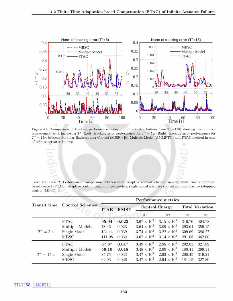
4.2 Finite Time Adaptation based Compensation (FTAC) of Infinite Actuator Failures
Time [s]0 20 40 60 80 100
‖x1−
yr‖
0
0.05
0.1
0.15
0.2
0.25
0.3
0.35
0.4Norm of tracking error (T∗=5)
30 35 40 45 50 55
0
0.05
0.1
MBSCMultiple ModelFTAC
Time [s]0 20 40 60 80 100
‖x1−
yr‖
0
0.05
0.1
0.15
0.2
0.25
0.3
0.35
0.4Norm of tracking error (T∗=15)
30 35 40 45 50 55
0
0.02
0.04
0.06
0.08
0.1 MBSCMultiple ModelFTAC
Figure 4.5: Comparison of tracking performance under infinite actuator failures Case 2 (4.118) showing performanceimprovement with increasing T ∗; (Left) tracking error performance for T ∗ = 5s; (Right) tracking error performance forT ∗ = 15s; between Modular Backstepping Control (MBSC) [6], Multiple Model (AMMFTC) and FTAC method in caseof infinite actuator failures
Table 4.2: Case 2: Performance Comparison between three adaptive control schemes, namely, finite time adaptationbased control (FTAC), adaptive control using multiple models, single model adaptive control and modular backsteppingcontrol (MBSC) [6]
Transit time Control SchemesPerformance metrics
ITAE RMSEControl Energy Total Variation
u1 u2 u1 u2
FTAC 95.04 0.023 3.67 × 10³ 3.15 × 10³ 316.76 404.78
T ∗ = 5 sMultiple Models 78.46 0.023 3.64 × 10³ 3.09 × 10³ 293.64 359.15Single Model 124.44 0.039 3.74 × 10³ 3.22 × 10³ 309.69 380.27MBSC 111.08 0.032 3.67 × 10³ 3.14 × 10³ 291.05 362.00
FTAC 57.87 0.017 3.49 × 10³ 2.98 × 10³ 202.63 327.89
T ∗ = 15 sMultiple Models 56.10 0.018 3.48 × 10³ 2.99 × 10³ 180.41 299.11Single Model 85.75 0.033 3.47 × 10³ 2.93 × 10³ 200.45 319.21MBSC 62.93 0.026 3.47 × 10³ 2.94 × 10³ 181.15 327.89
163
TH-2198_11610211

4. Finite Time Adaptation based Compensation (FTAC) of Actuator Failures in NonlinearUncertain Systems
Time [s]0 20 40 60 80 100
Out
put y
= ξ 2
-1.5
-1
-0.5
0
0.5
1
1.5
2
ξ2 yr
(a)
Time [s]0 20 40 60 80 100
Sta
te ξ 1
-8
-6
-4
-2
0
2
4
(b)
Time [s]0 20 40 60 80 100
Sta
te ξ 3
-6
-5
-4
-3
-2
-1
0
1
2
(c)
Time [s]0 20 40 60 80 100
Con
trol
inpu
ts
-10
-5
0
5
10
15
u1 u2
(d)
Figure 4.6: System states and control inputs for Case 2 (4.118) with T ∗ = 5s. (a) Output state ξ2 = x1;(b) state ξ1;(c)state ξ3 = x2; (d) control inputs u1 and u2
164
TH-2198_11610211

4.3 Finite Time Adaptation based Compensation (FTAC) of Actuator Failures inMulti-Input-Multi-Output (MIMO) Nonlinear Uncertain Systems
4.3 Finite Time Adaptation based Compensation (FTAC) of Actuator
Failures in Multi-Input-Multi-Output (MIMO) Nonlinear Uncer-
tain Systems
In this section, the proposed finite time adaptation based control (FTAC) strategy is extended to the
tracking control problem in MIMO nonlinear systems with immanent parametric uncertainties (totally
unknown system parameters) and abrupt actuator failures unknown in time pattern and magnitude. In
general, owing to the presence of strong coupling among inherent subsystems, the FTC design problem
for MIMO nonlinear systems and obtaining promising solutions, is certainly challenging. In the follow-
ing, an uncertain nonlinear dynamical system with multiple inputs and outputs incorporating actuator
failure input-output characteristics is described first. Thereafter, the adaptive FTC design with the
proposed finite time parameter estimator is put forward. Since, the inherent design assumptions for
the proposed control algorithm are essentially the same as in Chapter 3, Section 3.3.1, we restrain from
repeating the same herein to avoid repetition and preserve brevity of presentation all throughout this
chapter. Besides, the proposed finite time bound parameter estimation, the controller developed under
an indirect adaptive backstepping framework is exactly similar to what has been presented in (3.160)
(Section 3.3.2.1). Hence, the controller design procedure is not elucidated further. Instead, only some
of the important steps would be presented. Further, the stability analysis of the closed loop control
system under the action of the proposed control will be sketched briefly.
4.3.1 Problem Formulation
Let us consider the class of MIMO nonlinear systems affected by parametric uncertainties trans-
formed to a strict-feedback form as follows.
ξ1,r1 = ξ1,r1+1 +ϕT1,r1κ∗
ξ1,℘1 = a1(ξ, η) +ϕT1,℘1κ∗ +
m∑j=1
β1,j(ξ, η)uj(4.120)
...
ξq,rq = ξq,rq+1 +ϕTq,rqκ∗
ξq,℘q = aq(ξ, η) +ϕTq,℘qκ∗ +
m∑j=1
βq,j(ξ, η)uj(4.121)
η = Λ0(ξ,η) + ΛT1 (ξ,η)κ∗ (4.122)
y = [ξ1,1, ξ2,1, ξ3,1, . . . , ξi,1, . . . , ξq,1]T (4.123)
where ξ := [ξ1,1, ξ1,2, . . . , ξ1,℘1 , . . . , ξq,1, ξq,2, . . . , ξq,℘q ]T ∈ R
℘1+...+℘q denotes the state vector and ϕi,rifor i = 1, q and ri = 1, ℘i define the regressor matrices associated with unknown parameter vector
κ∗. The elements of the regressor matrices are linear and nonlinear smooth functions of the state
165
TH-2198_11610211

4. Finite Time Adaptation based Compensation (FTAC) of Actuator Failures in NonlinearUncertain Systems
vector ξ. The output of the system (4.120)-(4.121) is represented by the vector y = [yiqi=1]T ∈ R
q
while ℘1, ℘2, . . . , ℘q define the relative degrees of each of the q subsystems corresponding to their
outputs yi. The functions ai(ξ,η) for i = 1, q are known nonlinear smooth functions. The functions
βi,j(ξ,η) define the actuation functions for system dynamics corresponding to output yi with i = 1, q
and j = 1,m. The internal dynamics of the system are described by (4.122) and are assumed to be
ISS with respect to state vector ξ(t) as the input.
Undoubtedly, the actuators realizing the control inputs uj for j = 1,m are vulnerable to uncertain
faults and failures in their due course of operation over time. Similar to the actuator input-output
characterization presented in the previous chapters, the actuator failure model considered here is given
by,
uj =
KjuHj + uFj,
uHj,
∀ t ≥ tFj
∀ t < tFjj = 1,m (4.124)
The term uHj denotes the derived control signal to be fed as input to the jth actuator. While uFj
defines the value at which the jth actuator is stuck under stuck or lock-in-place (LIP) failure. The term
uFj=0 models float failure of the jth actuator. The factor Kj defines the partial loss of effectiveness
(PLOE) of the jth actuator. The actuator failures considered are unknown in time, pattern as well as
magnitude. The actuator index set is given by j1, j2, . . . , jm. It is assumed that the number of inputs
m is greater than the number of outputs q. Inspired from [32], the actuators are thereafter classified
under a grouping scheme G into q groups G1, . . . ,Gq according to their similarity in physical structure
and operational characteristics. This means that actuators reflecting the same physical structure and
functioning are placed together in a single group Gk ⊂ j1, j2, . . . , jm, k = 1, q. In other words, let us
assume that out of m actuators, mi of them exhibit similar operation and bear structural resemblance.
These mi actuators are allotted to group Gi and so on for i = 1, q. A proportional actuation scheme is
utilized similar to [32] to effectively exploit the actuator redundancy. Now, considering such a grouping
and actuation scheme G , the control input to be fed to each actuator included in the set Gk is given
by,
uHj = bjkvk ∀uj ∈ Gk, j = 1, m & k = 1, q (4.125)
where, bjk defines a certain known design function or constant associated with each actuator group Gk.
Further, the choice of such design functions satisfy the relation bjk = bj if the jth actuator belong to
Gk under the grouping scheme G .
Incorporating the actuator failure model in (4.124) along with the grouping G and a proportional
actuation scheme, the nonlinear uncertain system in (4.120)-(4.121) is reframed as,
ξ1,r1 = ξ1,r1+1 +ϕT1,r1κ∗
ξ1,℘1 = a1(ξ, η) +ϕT1,℘1κ∗ +
∑j∈j1,...,jd
β1,j(ξ, η)uFj +q∑
k=1
β1,k(ξ, η)vk(4.126)
166
TH-2198_11610211

4.3 Finite Time Adaptation based Compensation (FTAC) of Actuator Failures inMulti-Input-Multi-Output (MIMO) Nonlinear Uncertain Systems
ξ2,r2 = ξ2,r2+1 +ϕT2,r2κ∗
ξ2,℘2 = a2(ξ, η) +ϕT2,℘2κ∗ +
∑j∈j1,...,jd
β2,j(ξ, η)uFj +q∑
k=1
β2,k(ξ, η)vk(4.127)
...
ξq,rq = ξq,rq+1 +ϕTq,rqκ∗
ξq,℘q = aq(ξ, η) +ϕTq,℘qκ∗ +
∑j∈j1,...,jd
βq,j(ξ, η)uFj +q∑
k=1
βq,k(ξ, η)vk(4.128)
where βi,k :=∑
j 6∈j1,...,jd∩Gk
bjkKjβi,j(ξ,η) ∀k = 1, . . . , q and j = 1,m. The term uFj denotes the value
at which the jth actuator is stuck after it fails completely. The subscript d is delimited as d ≤ (m− q).To ensure that an adaptive control solution exists to compensate for the actuator faults and failures
apart from parametric uncertainties, the following condition must hold for a particular pattern of
actuator failure ∀ξ ∈ R℘1+...+℘q under the defined grouping scheme G .
det
β1,1 β1,2 . . . β1,q
β2,1 β1,2 . . . β2,q
.... . . . . .
...
βq,1 βq,2 . . . βq,q
G (Ξ)
6= 0. (4.129)
For the above condition to hold true for the grouping scheme G , a maximum of (mi−1) actuator failures
are allowed in each of the groups Gi. This condition ensures controllability of the nonlinear MIMO
system in presence of actuator faults and total failures; guaranteeing the existence of an adaptive
control solution to the FTC problem. The control design assumptions are fundamental and are no
different than what have been previously stated in Assumptions 3.9-3.10.
By virtue of all the necessary assumptions and the system dynamics under actuator faults/failures
described in (4.126)-(4.128), the control problem and its objectives are stated below.
• To design the control inputs vk for each of the actuator groups Gk with k = 1, q to ensure
boundedness of all closed loop signals.
• Adaptive estimation of unknown system parameters and actuator fault/failure induced paramet-
ric uncertainties in finite time, meaning limt→Ts
θ∗(t)− θ(t) = 0. Where θ∗ and θ denote the actual
parameter vector and its estimated equivalent, respectively. Ts defines the settling time.
• Asymptotic exponential convergence of the output tracking error (y−yr) to origin under nominal
(fault-free) conditions and in the event of actuator faults and failures unknown in their time of
occurrence, failure patterns and magnitudes, i.e., limt→∞
y(t) − yr(t) = 0.
• Improvement in output transient performance both at start up and post fault/failure scenarios
without any substantial increase in the control usage. Unknown subsystem interactions in MIMO
nonlinear systems are known play a decisive role in determining the system output transient
167
TH-2198_11610211

4. Finite Time Adaptation based Compensation (FTAC) of Actuator Failures in NonlinearUncertain Systems
behavior. Thus, reinforced robustness towards consequences of unknown strong cross coupling
effects arising from such interactions is an additional design objective to be accomplished.
4.3.2 Proposed Finite Time Adaptation based Controller (FTAC)
Prior to the proposed controller design, the faulty system in (4.126)-(4.128) is first parameter-
ized to identify the unknown parameters associated with actuator faults and failures. Following the
parametrization, the unknown system parameters are represented by θ∗2 = κ∗; while large paramet-
ric uncertainties introduced into the system due to occurrence of actuator failures are defined as
θ∗1 = [θ∗1,1, . . . , θ∗1,m]T = [K1,K2, . . . ,Km]T and θ∗3 = [θ∗3,1, . . . , θ
∗3,m]T = [uF1, uF2, . . . , uFm]T . Af-
ter the preceding definitions, the vector comprising of all the aforementioned unknown parameters is
defined as θ∗ := [θ∗1, θ∗2, θ
∗3]T . In what follows, the controller design is presented which helps in
realizing the “modularity" between control and parameter estimation thereby guaranteeing a unidirec-
tional interaction between the controller-observer pair as desired. Thereafter, the parameter estimator
featuring finite time convergence of the parameter estimation error to the origin is proposed. It is
worth mentioning that the adaptive parameter estimator to be proposed in the sequel is independent
of the boundedness of the regressor vector and hence the signals associated with the estimation module
are bounded.
4.3.2.1 Controller Synthesis
Let us first augment all the q inputs denoted by vk for k = 1, q together to form the vector
v := [v1, v2, . . . , vq]T . Now, the design of v(t) entirely follows the same procedure in Chapter 3
(Section 3.3.2.1). Thus, only some important steps are provided for the sake of completeness. Firstly,
the following error variables are introduced.
z1,1 = ξ1,1 − yr,1; z1,r1 = ξ1,r1 − α1,r1−1 − y(r1−1)r,1 ;
z2,1 = ξ2,1 − yr,2; z2,r2 = ξ2,r2 − α2,r2−1 − y(r2−1)r,2 ;
......
zq,1 = ξq,1 − yr,q; zq,rq = ξq,rq − αq,rq−1 − y(rq−1)r,q (4.130)
where ri = 2, ℘i, i = 1, q, y(ri−1)r,i denotes (ri − 1)th derivative of the ith reference signal yr,i and αi,ri
are the stabilizing control laws known as virtual inputs determined at the rthi step (for ri = 1, ℘i − 1)
as
αi,1 = −ci,1zi,1 − ci,1‖ψi,1‖2zi,1 −ϕTi,1θ2 (4.131)
αi,ri = −zi,ri−1 − ci,rizi,ri −
ci,ri‖ψi,ri‖2 + gi,ri
∥∥∥∥∥∂αi,ri−1
∂θ2
∥∥∥∥∥
2
zi,ri −ψTi,riθ2
+
(ri−1∑
k=1
∂αi,ri−1
∂ξi,kξi,k+1 +
ri−1∑
k=1
∂αi,ri−1
∂yk−1r,i
y(k)r,i
). (4.132)
168
TH-2198_11610211

4.3 Finite Time Adaptation based Compensation (FTAC) of Actuator Failures inMulti-Input-Multi-Output (MIMO) Nonlinear Uncertain Systems
Where, ψi,ri = ϕi,ri −ri−1∑k=1
∂αi,ri−1
∂ξi,kϕi,k for i = 1, q and ri = 2, ℘i − 1. The actual control input v(t) is
then derived to be
v(t) =
βm∑
j=1
θ1,jNjB
−1
−a1(ξ, η) −ψT1,℘1θ2 − β1θ3 − z1,℘1−1 + Fξ1 + Fr,1 + y
(℘1)r,1
−a2(ξ, η) −ψT2,℘2θ2 − β2θ3 − z2,℘2−1 + Fξ2 + Fr,2 + y
(℘2)r,2
...
−aq(ξ, η) −ψTq,℘qθ2 − βqθ3 − zq,℘q−1 + Fξq + Fyr,q + y
(℘q)r,q
+
(ℓβB
)−1
−c1,℘1z1,℘1 − c1,℘1(‖ψ1,℘1‖2 + ‖β1‖2 + ‖β1u‖2)z1,℘1 − g1,℘1
∥∥∥∥∥∂α1,℘1−1
∂θ2
∥∥∥∥∥
2
z1,℘1
−c2,℘2z2,℘2 − c2,℘2(‖ψ2,℘2‖2 + ‖β2‖2 + ‖β2u‖2)z2,℘2 − g2,℘2
∥∥∥∥∥∂α2,℘2−1
∂θ2
∥∥∥∥∥
2
z2,℘2
...
−cq,℘qzq,℘q − cq,℘q(‖ψq,℘q‖2 + ‖βq‖2 + ‖βqu‖2)zq,℘q − gq,℘q
∥∥∥∥∥∂αq,℘q−1
∂θ2
∥∥∥∥∥
2
zq,℘q
(4.133)
. Wherein the terms have their respective meanings with
Fξ =
℘1−1∑
k=1
∂α1,℘1−1
∂ξ1,kξ1,k+1,
℘2−1∑
k=1
∂α2,℘2−1
∂ξ2,kξ2,k+1, . . . ,
℘q−1∑
k=1
∂αq,℘q−1
∂ξq,kξq,k+1
T
Fyr(yr, yr, . . . ,y
(℘)r ) =
℘1−1∑
k=1
∂α1,℘1−1
∂y(k−1)r,1
y(k)r,1 ,
℘2−1∑
k=1
∂α2,℘2−1
∂y(k−1)r,2
y(k)r,2 , . . . ,
℘q−1∑
k=1
∂αq,℘q−1
∂y(k−1)r,q
y(k)r,q
T
β(ξ,η) := [β1(ξ,η), β2(ξ,η), . . . , βq(ξ,η)]T ∈ Rq×m
Further, Nj ∈ Rm×m is a square matrix with the jth element on the main diagonal being 1 and all
other entries as 0. While the known proportional actuation matrix B and βu are defined as
B :=
b11 . . . b1q...
. . ....
bm1 . . . bmq
; βu =
β1,1uH1 β1,2uH2 . . . β1,muHm
. . . . . .... . . .
βq,1uH1 βq,2uH2 . . . βq,muHm
.
and βiu denotes the ith row vector of the matrix βu. θ1, θ2 and θ3 are the estimates of the unknown
parameters θ∗1, θ∗2 and θ∗2 , respectively. It has been mentioned earlier that one actuator in each group
Gk, k = 1, q under the grouping scheme G should be alive to satisfy the controllability condition in
(4.129). Thus, the assumption ‖θ∗‖ > ℓ and hence
∥∥∥∥∥m∑j=1
θ∗1,jNj
∥∥∥∥∥ > ℓ with ℓ > 0 is justified. The
parameter estimates are obtained from a faithful finite time bound estimator with θ = θ∗ − θ = 0
within an explicitly calculated finite time Ts. The design of the estimator will be discussed in the
169
TH-2198_11610211

4. Finite Time Adaptation based Compensation (FTAC) of Actuator Failures in NonlinearUncertain Systems
section hereafter.
4.3.2.2 Design of Parameter Estimator with Finite Time Convergence
Firstly, the design of the parameter estimator requires the nonlinear system dynamics in (4.126)-
(4.128) to be represented as a parametric ξ model as given below.
ξ1,1...
ξq,1...
ξ1,℘1
...
ξq,℘q
︸ ︷︷ ︸ξ
=
ξ1,2...
ξq,2...
a1(ξ, η)...
aq(ξ, η)
︸ ︷︷ ︸a(ξ,η)
+
0 . . . 0 ϕT1,1 0...
......
......
0 . . . 0 ϕTq,1 0...
.... . .
......
β1,1uH1 . . . β1,muHm ϕT1,℘1β1
.... . .
......
...
βq,1uH1 . . . βq,muHm ϕTq,℘qβq
θ∗1,1...
θ∗1,mθ∗2θ∗3
︸ ︷︷ ︸ΦT (ξ,u)θ∗
(4.134)
Where uHj :=q∑
k=1
bjkwk for j = 1,m. From (4.134), it can be well observed that the structure of
the above estimation model is essentially the same as (4.12) regardless of the number of inputs and
outputs of the system. In view of an exactly similar structural description of the parametric ξ−model,
the parameter estimator along with the necessary prerequisite filters are stated with direct reference
from Section 4.2.3.1. Further, the convergence properties of the filtered signals, as we would observe
in the sequel, will essentially follow from the results deduced in Lemmas 4.1-4.5 and Proposition 4.1.
Let us therefore introduce the necessary filters as
ΩT = A(ξ, t)ΩT + ΦT (x,v); Ω ∈ R(2m+p)×
∑k ℘k (4.135)
Ω0 = A(ξ, t)(Ω0 + ξ) − a(ξ); Ω0 ∈ R
∑k ℘k (4.136)
Where k = 1, q and A(ξ, t) = A0 − γΦT (x,v)Φ(x,v)P. Further, A0 is a constant Hurwitz matrix
with a positive definite matrix P = PT > 0 as the solution to the equality A0TP+PA0 +Q = 0 with
a chosen Q > 0. Additionally, we define another two filters with filtered variables R(t) and S(t) as,
R(t) = −K R(t) + ΩΩT ; R(0) = 0, R(t) ∈ R(2m+p)×(2m+p) (4.137)
S(t) = −K S(t) + Ω(Ω0 + ξ); S(0) = 0, S(t) ∈ R2m+p (4.138)
where K > 0 is another design scalar. Thereafter, defining the prediction error as E := S(t)−R(t)θ,
the parameter update law exhibiting finite time stable solutions is obtained as follows.
˙θ = Γ1
E (t)
‖E (t)‖1/2+ Γ2
t∫
0
E (s)
‖E (s)‖ds (4.139)
170
TH-2198_11610211

4.3 Finite Time Adaptation based Compensation (FTAC) of Actuator Failures inMulti-Input-Multi-Output (MIMO) Nonlinear Uncertain Systems
Herein Γ1,Γ2 > 0 define the rate of adaptation and decides the speed of convergence of the parameter
estimates to their actual values. The following proposition, the stability properties of the proposed
finite time parameter estimator and other auxiliary signals are summarized.
Proposition 4.2. Let us assume that the regressor Φ(ξ,u) in the estimation model (4.134) is PE such
that the solution of (4.137) given by R(t) is positive definite. Thus, the proposed adaptive parameter es-
timation law described by (4.139) ensures the finite time convergence of the parameter estimation error
θ to the origin from any initial condition. Further, the convergence time is defined by a explicit settling
time function Ts(θ(t0 = 0), t0 = 0) dependent on initial conditions and satisfies 0 ≤ Ts(θ(0), 0) < +∞.
In addition, the following properties hold in the sense of the solutions of (4.139); (i) θ(t) ∈ L1 ∩ L∞and (ii)
˙θ(t) ∈ L1.
Proof.
Proving finite time stability of θ = 0 and the derivation of the settling time function Ts follows the
same procedure as in the proof of Proposition 4.1 (i). Hence the proof is straightforward and the
results directly follow from Proposition 4.1 (i). Nevertheless, the important milestones of the proof are
provided in the succeeding text for ease of understanding.
To prove finite time stability, a new vector is defined as θ :=
[θ
‖θ‖ 12
, θa
]T. Where θa = −Γ2
t∫0
E (s)
‖E (s)‖ds
is an auxiliary state variable. The Lyapunov function candidate VΘ
: R2(2m+p) \ 0 × [0,∞) → R+ as
(Θ, t) 7→ ΘTPΘ with P > 0 as a symmetric matrix. Thereafter taking the first time derivative of VΘ
and following similar steps as in the proof of Proposition 4.1 (i), results in
VΘ
≤ −Γ√VΘ< 0 (4.140)
where Γ =λ
12 (P)λ(Q)
λ(P), λ(·) and λ(·) denote the maximum and minimum eigen values of a square
matrix. The matrix Q = −(FTP + PF) and F =1
2
−λ(R)√λ(R)
Γ1 I2m+p
−2λ(R)
λ(R)Γ2 02m+p
Invoking Theorem
2.1 in [106] and from the inequality obtained in (4.140), finite time stability of Θ = 0 is proved. The
derivation of the expression for settling time Ts follows from inequality (4.140). For any initial condition
VΘ
(t0 = 0) = VΘ
(0), the time taken by Θ(t) to converge to the origin is atmost Ts = 2VΘ
(0)12 /Γ
seconds. Thus, the first part of the proof is complete.
In the proof above, θ∗ is considered to be constant vector. However, occurrence of actuator failures
will result in θ∗ 6= 0 at failure instances. Herein, we are interested in inferring the stability properties
of signals for all 0 ≤ t < ∞ instead of concluding about their piecewise characteristics with respect
to time. It has already been explained in Remark 4.1 that θ∗ is L1-integrable provided the number
of changes in the unknown parameter vector due to actuator failures is finite. From Lemma 4.2, the
171
TH-2198_11610211

4. Finite Time Adaptation based Compensation (FTAC) of Actuator Failures in NonlinearUncertain Systems
boundedness of Ω is inferred. The solution R(t) of the matrix differential equation (4.137) is given by
R(t) ≤ R(0)e−K I2m+pt ‖Ω(t)‖2∞
K(eK I2m+pt − I2m+p) ≤
‖Ω(t)‖2∞
KI2m+p <∞ (4.141)
Hence, ‖R(t)‖∞ =√
2m+ p‖Ω(t)‖2∞/K and R(t), R(t) ∈ L∞. To prove θ ∈ L1, the signal Θ to be
L1-integrable. Thus, with θ∗ 6= 0 the expression of VΘ
takes the following form.
VΘ
≤ −Γ√λ(P)︸ ︷︷ ︸Γ
‖Θ‖ + λ(P)‖θ∗‖ (4.142)
Therefore, integrating the immediately above inequality and subsequent application of H0lder’s in-
equality from 0 ∼ ∞ yields,
∞∫
0
VΘds ≤ −Γ
∞∫
0
‖Θ‖ds + λ(P)
∞∫
0
‖θ∗‖ds (4.143)
∞∫
0
‖Θ‖ds ≤ λ(P)√λ(P)Γ
‖Θ(0)‖2 +λ(P)
Γ√λ(P)
∞∫
0
‖θ∗‖ds (4.144)
From inequality (4.144) and invoking θ∗ ∈ L1, the L1-integrability of Θ is concluded. Therefore
θ, θa ∈ L1 ∩ L∞ follows. Further, since R(t), R(t) ∈ L∞, it is straightforward to prove˙θ ∈ L1. The
proof is complete.
4.3.3 Stability Analysis of the Proposed Control System
The stability properties of the closed loop signals under the proposed control scheme are summarized
in Theorem 4.4. Prior to the theoretical conclusions on the convergence features offered by the proposed
control scheme; let us first reiterate the tracking error dynamics of the closed loop controlled system.
The closed loop tracking error dynamics is described by
z = Az(z, θ, t)z + Bθ∗(z, θ, t)θ + B ˙θ(z, θ, t)
˙θ. (4.145)
Where z(t) := [z1,1, z2,1, . . . , zq,1, z1,2, z2,2, . . . , zq,2, . . . , z1,℘1 , z2,℘2 , . . . , zq,℘q ]T = [zTi,1, zTi,2, . . . , zTi,q]
T
for i = 1, q and the matrices Az is defined in (4.152), respectively. The matrices Bθ∗ and B ˙θ
are
172
TH-2198_11610211

4.3 Finite Time Adaptation based Compensation (FTAC) of Actuator Failures inMulti-Input-Multi-Output (MIMO) Nonlinear Uncertain Systems
defined as follows.
Bθ∗ :=
0 0 . . . 0
0 0 . . . 0...
. . .. . .
...
0 . . . . . . 0
ψT1,1...
ψTq,1
0 0 . . . 0
0 0 . . . 0...
. . .. . .
...
0 . . . . . . 0
0 0 . . . 0
0 0 . . . 0...
. . .. . .
...
0 . . . . . . 0
ψT1,2...
ψTq,2
0 0 . . . 0
0 0 . . . 0...
. . .. . .
...
0 . . . . . . 0...
......
0 0 . . . 0
0 0 . . . 0...
. . .. . .
...
0 . . . . . . 0
ψT1,℘1−1...
ψTq,℘q−1
0 0 . . . 0
0 0 . . . 0...
. . .. . .
...
0 . . . . . . 0
β1,1uH1 . . . β1,muHm...
. . ....
βq,1uH1 . . . βq,muHm
ψT1,℘1
...
ψTq,℘q
β1,1 . . . β1,m
.... . .
...
βq,1 . . . βq,m
B ˙θ2
:= −[
0∂α1,1
∂θ2
. . .∂αq,1
∂θ2
. . .∂α1,℘1−1
∂θ2
. . .∂αq,℘q−1
∂θ2
]T(4.146)
The matrix in left most lower block of the matrix Bθ∗ is denoted by
βu := [β1u, β
2u, . . . , β
qu]T =
β1,1uH1 . . . β1,muHm
β2,1uH1 . . . β2,muHm...
. . ....
βq−1,1uH1 . . . βq−1,muHm
βq,1uH1 . . . βq,muHm
.
Such a notation is preferred to lend simplicity in matrix calculations to follow in the sequel. The closed
loop system matrix and the relevant input matrices with reference to (4.145), namely, Az, Bθ∗ and
B ˙θ2
are of orderq∑i=1
℘i ×q∑i=1
℘i,q∑i=1
℘i × (2m + p) andq∑i=1
℘i × p with elements from R. Further, the
shorthand notation used to represent the elements of the matrix Az is explained as, ai,j := ci,j + si,j
for i = 1, q and j = 1, ℘q. The terms ci,j are constant controller gains and the damping factors si,j are
173
TH-2198_11610211

4. Finite Time Adaptation based Compensation (FTAC) of Actuator Failures in NonlinearUncertain Systems
defined as,
s1,1 = c1,1‖ψ1,1‖2 (4.147)
s1,r1 = c1,r1‖ψ1,r1‖2 + g1,r1
∥∥∥∥∂α1,r1−1
∂θ2
∥∥∥∥2
, r1 = 2, ℘1 − 1 (4.148)
s1,℘1 = c1,℘1(‖ψ1,℘1‖2 + ‖β1‖2 + ‖v1‖2) + g1,℘1
∥∥∥∥∂α1,℘1−1
∂θ2
∥∥∥∥2
(4.149)
. . . . . .
si,ri = ci,ri‖ψi,ri‖2 + gi,ri
∥∥∥∥∂αi,ri−1
∂θ2
∥∥∥∥2
, ri = 2, ℘i − 1, i = 1, q (4.150)
si,℘i = ci,℘i(‖ψi,℘i‖2 + ‖βi‖2 + ‖vi‖2) + gi,℘i
∥∥∥∥∂αi,℘i−1
∂θ2
∥∥∥∥2
(4.151)
In what follows, the theorem states the stability characteristics of the closed loop signals when the
system is affected by finite number of actuator failures. By finite number of actuator failures, we mean
that the system can be subjected to a maximum of (m−q) actuator failures satisfying (4.129) to enable
the existence of an adaptive FTC strategy to recover its performance.
Theorem 4.4. Let us consider the MIMO nonlinear uncertain system dynamics in (4.126)-(4.128)
with unknown parameters, affected by finite number of actuator failures. Considering the immanent
design assumptions 3.8-3.10, the proposed adaptive controller (4.133) augmented with the finite time
parameter estimator in (4.139) renders the following properties with the maximal interval of existence
of signals being [0,∞).
(i) All closed loop signals have stable trajectories and z(t) ∈ L∞.
(ii) The tracking error vector z(t) ∈ L1 and the output tracking error asymptotically converges to the
origin, i.e., limt→∞
(y − yr) = 0.
174
TH-2198_11610211

4.3
Fin
iteT
ime
Adapta
tion
base
dC
om
pensa
tion
(FTA
C)
ofA
ctu
ato
rFailu
res
inM
ulti-In
put-M
ulti-O
utp
ut
(MIM
O)
Nonlin
ear
Uncerta
inSyste
ms
Az :=
−a11 0 . . . 0
0 −a21 . . . 0...
. . .. . .
...
0 . . . . . . −aq1
1 0 . . . 0
0 1 . . . 0...
. . .. . .
...
0 . . . . . . 1
0 0 . . . 0
0 0 . . . 0...
. . .. . .
...
0 . . . . . . 0
. . .
0 0 . . . 0
0 0 . . . 0...
. . .. . .
...
0 . . . . . . 0
−1 0 . . . 0
0 −1 . . . 0...
. . .. . .
...
0 . . . . . . −1
−a12 0 . . . 0
0 −a22 . . . 0...
. . .. . .
...
0 . . . . . . −aq2
1 0 . . . 0
0 1 . . . 0...
. . .. . .
...
0 . . . . . . 1
. . .
0 0 . . . 0
0 0 . . . 0...
. . .. . .
...
0 . . . . . . 0
.... . .
. . .. . .
......
. . .. . .
. . ....
.... . .
. . .. . .
1 0 . . . 0
0 1 . . . 0...
. . .. . .
...
0 . . . . . . 1
0 0 . . . 0
0 0 . . . 0...
. . .. . .
...
0 . . . . . . 0
0 0 . . . 0
0 0 . . . 0...
. . .. . .
...
0 . . . . . . 0
. . .
−1 0 . . . 0
0 −1 . . . 0...
. . .. . .
...
0 . . . . . . −1
−β∑j
θ∗1,j Nj β
†
ℓ
a1℘1. . . 0
.... . .
...
0 . . . aq℘q
(4.152)
175
TH-2198_11610211

4. Finite Time Adaptation based Compensation (FTAC) of Actuator Failures in NonlinearUncertain Systems
Proof of (i).
From Proposition 4.2, the boundedness of θ and˙θ ∈ L1 is proved. Thereafter following exactly similar
steps as in the proof of Theorem 3.8(i) with the substitution θs = θ yields the following.
1
2
d
dt
(q∑
i=1
℘i∑
ri=1
z2i,ri
)≤ −
q∑
i=1
℘i−1∑
ri=1
ci,riz2i,ri +
q∑
i=1
ci,℘iz2i,℘i
+1
4
(‖θ1‖2
¯c+
‖θ2‖2
c+
‖θ3‖2
4¯c+
‖ ˙θ2‖2
g
)
(4.153)
≤ −q∑
i=1
℘i∑
ri=1
ci,riz2i,ri +
1
4
(‖θ‖2
c+
‖ ˙θ2‖2
g
)(4.154)
≤ −2C
q∑
i=1
℘i∑
ri=1
z2i,ri +
1
4
(‖θ‖2
c+
‖ ˙θ2‖2
g
)(4.155)
where ¯c =
(q∑i=1
1ci,℘i
)−1
, c =
(q∑i=1
℘i∑ri=1
1ci,ri
)−1
, g =
(q∑i=1
℘i∑ri=2
1gi,ri
)−1
, c = min¯c, c and C =
min1≤i≤q
1≤ri≤℘i
ci,ri. Invoking the boundedness of θ and˙θ ∈ L1 in (4.155), directs the conclusion that
z(t) ∈ L∞.
Proof of (ii).
The closed loop tracking error dynamics is first rewritten as,
z(t) = Az(z, θs, t)z(t) + Bθ∗(z, θs, t)θs + B ˙θ2
(z, θs, t)˙θ2s (4.156)
where the matrices Az and Bθ∗ are defined in (4.159)-(4.160). The matrix B ˙θ2
has the same definition
as given in (4.146). Needless to mention, the procedure to arrive at the L1−integrability of the tracking
error vector z(t), although not trivial is same as what has been followed in the proof of Theorem 4.2 (ii)
with slight modifications. The essential steps are mentioned herein to abstain from a too comprehensive
treatment and more importantly to avert redundant calculations.
Let us begin by introducing an auxiliary state variable χT ∈ R
∑k ℘k×(2m+p) whose dynamics are
described by the following matrix differential equation,
χT = Az(z, θ, t)χT + Bθ∗(z, θ, t) (4.157)
The solution of (4.157) is described by
χT = e−AztχT (0) +
t∫
0
e−Az(t−s)Bθ∗(s)ds (4.158)
176
TH-2198_11610211

4.3
Fin
iteT
ime
Adapta
tion
base
dC
om
pensa
tion
(FTA
C)
ofA
ctu
ato
rFailu
res
inM
ulti-In
put-M
ulti-O
utp
ut
(MIM
O)
Nonlin
ear
Uncerta
inSyste
ms
Az :=
−a11 0 . . . 0
0 −a21 . . . 0...
. . .. . .
...
0 . . . . . . −aq1
1 0 . . . 0
0 1 . . . 0...
. . .. . .
...
0 . . . . . . 1
0 0 . . . 0
0 0 . . . 0...
. . .. . .
...
0 . . . . . . 0
. . .
0 0 . . . 0
0 0 . . . 0...
. . .. . .
...
0 . . . . . . 0
−1 0 . . . 0
0 −1 . . . 0...
. . .. . .
...
0 . . . . . . −1
−a12 0 . . . 0
0 −a22 . . . 0...
. . .. . .
...
0 . . . . . . −aq2
1 0 . . . 0
0 1 . . . 0...
. . .. . .
...
0 . . . . . . 1
. . .
0 0 . . . 0
0 0 . . . 0...
. . .. . .
...
0 . . . . . . 0
.... . .
. . .. . .
......
. . .. . .
. . ....
.... . .
. . .. . .
1 0 . . . 0
0 1 . . . 0...
. . .. . .
...
0 . . . . . . 1
0 0 . . . 0
0 0 . . . 0...
. . .. . .
...
0 . . . . . . 0
0 0 . . . 0
0 0 . . . 0...
. . .. . .
...
0 . . . . . . 0
. . .
−1 0 . . . 0
0 −1 . . . 0...
. . .. . .
...
0 . . . . . . −1
−β∑j
θ1,j Nj β†
ℓ
a1℘1. . . 0
.... . .
...
0 . . . aq℘q
(4.159)
Bθ∗ :=
0 0 . . . 0
0 0 . . . 0...
. . .. . .
...
0 . . . . . . 0
ψT1,1...
ψTq,1
0 0 . . . 0
0 0 . . . 0...
. . .. . .
...
0 . . . . . . 0...
......
β1,1uH1 . . . β1,muHm...
. . ....
βq,1uH1 . . . βq,muHm
ψT1,℘1
...
ψTq,℘q
β1,1 . . . β1,m
.... . .
...
βq,1 . . . βq,m
(4.160)
177
TH-2198_11610211

4. Finite Time Adaptation based Compensation (FTAC) of Actuator Failures in NonlinearUncertain Systems
Using the inequality ‖e−Azt‖ ≤ ˘ke−c0t, c0,
˘k > 0 in (4.158) and the fact that Bθ∗ is bounded (since
all closed loop trajectories are bounded) results in
‖χ‖ ≤ ‖χ(0)‖ +˘k‖Bθ∗‖∞
c0(4.161)
Hence the auxiliary state variable χT (t) ∈ L∞ is ascertained from (4.161). At this point, let us define
another additional variable ϑ as follows
ϑ(t) = z(t) − χT θ(t) (4.162)
Thus from the definition of ϑ(t), to prove that z(t) ∈ L1 requires ϑ(t) and χT θ(t) to be L1−integrable.
Proving χT θ ∈ L1 is straightforward as shown below. Integrating ‖χT θ‖ from t = 0 ∼ ∞ and
thereafter applying Hölder’s inequality to the integral results in,
∞∫
0
‖χT θ‖dt ≤ ‖χ‖∞∞∫
0
‖θ‖ds (4.163)
The above inequality uses the boundedness of χ(t) derived in (4.161). Further θ(t) ∈ L1 is proved in
Proposition 4.2. Hence χT θ ∈ L1 follows from (4.163).
Now what remains is to prove ϑ(t) ∈ L1. It should be reiterated that all the signal properties are
derived considering their maximal interval of existence to be [0,∞). Adopting similar calculations as
in (4.82), the following dynamics of ϑ(t) is arrived at,
ϑ = Azϑ+ B ˙θ2
˙θ2 + χT
˙θ − χT θ∗ (4.164)
The solution of (4.164) is derived to be
ϑ(t) = e−Aztϑ(0) +
t∫
0
e−Az(t−s)B ˙θ2
(z(s), θ(s), s)˙θ2(s)ds
+
t∫
0
e−Az(t−s)χT (s)˙θ(s)ds −
t∫
0
e−Az(t−s)χT (s)θ∗(s)ds (4.165)
Thereafter imposing the norm operator on both sides of (4.165) and using the inequality ‖e−Azt‖ ≤
178
TH-2198_11610211

4.3 Finite Time Adaptation based Compensation (FTAC) of Actuator Failures inMulti-Input-Multi-Output (MIMO) Nonlinear Uncertain Systems
˘ke−c0t, c0,
˘k > 0 followed by Hölder’s inequality, leads to
‖ϑ(t)‖ ≤ ˘ke−c0t‖ϑ(0)‖︸ ︷︷ ︸
I
+˘k‖B ˙
θ‖∞
t∫
0
e−c0(t−s)‖ ˙θ(s)‖ds
︸ ︷︷ ︸II
+˘k‖χ‖∞
t∫
0
e−c0(t−s)‖ ˙θ(s)‖ds
︸ ︷︷ ︸III
+˘k‖χ‖∞
t∫
0
e−c0(t−s)‖θ∗(s)‖ds
︸ ︷︷ ︸IV
(4.166)
Now integrating both sides of inequality (4.166) from t ∼ t+ T and thereafter calculating the integral
to be finite would prove the claim. The integrals of I-IV are calculated in the same order as stated
above for clarity. The integral of I is calculated to be
t+T∫
t
˘ke−c0s‖ϑ(0)‖ds =
˘k
c0‖ϑ(0)‖ <∞. (4.167)
Integration of II in(4.166) from t ∼ t+ T leads to the following.
t+T∫
t
˘k‖B ˙
θ2‖∞
s∫
0
e−c0(s−τ)‖ ˙θ2(τ)‖dτds ≤ ˘
k‖B ˙θ2‖∞
t+T∫
t
s∫
0
e−c0(s−τ)‖ ˙θ2(τ)‖dτds
≤ ˘k‖B ˙
θ2‖∞
t+T∫
t
e−c0st∫
0
ec0τ‖ ˙θ2(τ)‖dτds +
˘k‖B ˙
θ2‖∞
t+T∫
t
e−c0ss∫
t
ec0τ‖ ˙θ2(τ)‖dτds
≤˘k‖B ˙
θ2‖∞
c0
t∫
0
e−c0(t−τ)‖ ˙θ2(τ)‖dτ +
˘k‖B ˙
θ2‖∞
t+T∫
t
e−c0ss∫
t
ec0τ‖ ˙θ2(τ)‖dτds (4.168)
Inequality (4.168) is derived using the property e−c0t − e−c0(t+T ) ≤ e−c0t. The first expression on the
right hand side of the last inequality among the set of inequalities in (4.87) can be solved using the
procedure adopted in [110] (Chapter 3, page 85) to arrive at the boundedness of ∆. Using the fact that˙θ2 ∈ L1 (instead of S1(ν) since finite number of actuator failures are considered), and if its L1−bound
is designated by ‖ ˙θ2‖L1 the result below follows,
˘k‖B ˙
θ2‖∞
c0
t∫
0
e−c0(t−τ)‖ ˙θ2(τ)‖dτ ≤
˘k‖B ˙
θ2‖∞ec0
c0(1 − e−c0)‖ ˙θ2‖L1 <∞ (4.169)
Having determined the boundedness of the integral in (4.169), proving the finiteness of the remaining
integral on the RHS of (4.168) is yet to be attempted. In this direction, the identity for the change of
179
TH-2198_11610211

4. Finite Time Adaptation based Compensation (FTAC) of Actuator Failures in NonlinearUncertain Systems
sequence of integration (4.37) is applied to the underlying integral as shown below.
˘k‖B ˙
θ2‖∞
t+T∫
t
e−c0ss∫
t
ec0τ‖ ˙θ2(τ)‖dτds =
˘k‖B ˙
θ2‖∞
t+T∫
t
ec0τ‖ ˙θ2(τ)‖
t+T∫
τ
e−c0sdsdτ
≤˘k‖B ˙
θ2‖∞
c0
t+T∫
t
‖ ˙θ2(τ)‖dτ (4.170)
(4.171)
Let us now consider the limits of the integral on the RHS of (4.170) in accordance with t = 0 and
T → ∞. Thereafter invoking the L1−integrability property of˙θ proved earlier, the boundedness of
(4.170) follows, that is,
˘k‖B ˙
θ2‖∞
t+T∫
t
e−c0ss∫
t
ec0τ‖ ˙θ2(τ)‖dτds <∞ (4.172)
Hence the integral of II is proved to have a finite bound. Eventually, since the integral of III and
IV looks similar to that of II, the same procedure is followed to arrive at their boundedness. The
derivation procedure involves the slicing of the interval [0, s] to [0, t] and [t, s] and solving two resultant
integrals using change of sequence of integration. The L1−integrability property of˙θ and θ∗ is invoked
thereafter to infer the boundedness of the underlying integrals. The steps are indeed straightforward
if the reader is familiar with the boundedness calculations culminating in (4.172). Hence for the sake
of conciseness the proof is not repeated. Thus, from the foregoing arguments and discussions, it is
mathematically proved that ϑ(t) ∈ L1 from its inequality definition in (4.166). Now from the property
of closed under addition of function spaces, since z(t) = ϑ(t) + χT θ(t), the signal property z(t) ∈ L1
is proved.
4.3.4 Simulation Study
To demonstrate the effectiveness of the proposed adaptive FTC approach featuring finite time
adaptation, simulations are conducted on a coupled mass-spring-damper (MSD) system. The mass-
spring-damper system taken into consideration is shown in Figure (3.13). Certainly, this system serves
as a benchmark example of a nonlinear coupled MIMO dynamical system to validate the applicability
and beneficial attributes of several nonlinear control schemes. The system description and modeling
have been detailed in Section 3.3.4 in the previous chapter and hence not repeated.
Referring to the nonlinear uncertain dynamics of the coupled mass-spring-damper system in (3.213), the
parameters of the system are the same as considered in the previous chapter. Further, the unknown
failure induced uncertainty parameters are considered to be the same for simulations in order to
ensure similar operating conditions necessary for comparison. The following actuator failure condition
180
TH-2198_11610211

4.3 Finite Time Adaptation based Compensation (FTAC) of Actuator Failures inMulti-Input-Multi-Output (MIMO) Nonlinear Uncertain Systems
considered reflects their partial loss of effectiveness (PLOE).
u1(t) =
0.5uH1, t ≥ 30s
uH1, otherwise(4.173)
u2(t) =
0.5uH2, t ≥ 60s
uH2, otherwise(4.174)
In order to translate the control design procedure to the system concerned, the dynamics in (3.213) is
represented in a more appropriate form as
ξ1 = ξ2 (4.175)
ξ2 = ϕTθ∗2 +2∑
j=1
θ∗1,jNjuH . (4.176)
Where the state vector ξ := [ξ1, ξ2], ξ1 := [ξ1,1, ξ2,1]T , ξ2 := [ξ1,2, ξ2,2]
T the entire dynamical system
is rewritten asϕT := [diagϕT1,2, ϕT2,2]T and uH = [uH1, uH2]T . The regressor matrices are defined
as ϕ1,2 := [−ξ1,1, −ξ31,1, −ξ1,2, −ξ21,2, (ξ2,2− ξ1,2), (ξ2,2 − ξ1,2)2]T and ϕ2,2 := [−(ξ2,1− ξ1,1), −(ξ2,1 −ξ1,1)
3, −ξ1,2, −ξ21,2]T . Further, the estimation model for the considered nonlinear dynamical system
(3.213) is formulated as
ξ =
ξ1,2
ξ2,2
0
0
+
0 01×6 0 01×4
0 01×6 0 01×4
uH1 ϕT1,2 0 01×4
01×9 01×6 uH2 ϕT2,2
︸ ︷︷ ︸ΦT
θ∗. (4.177)
Herein θ∗ := [θ∗1,1, θ∗2,1, . . . , θ
∗2,8, θ1,2, θ2,9, . . . , θ2,12]
T . The reference trajectories to be tracked by the
outputs y1 = ξ1,1 and y2 = ξ2,1 are given by yr,1 = 0.2 sin(0.5t) and yr,2 = 0.5 sin(0.5t). The controllers
uH1 and uH2 are developed consistent with equation (4.133) and the parameter estimation θ follows
(4.135) through (4.139). Unlike the control algorithm proposed in the previous chapter, there is only
one single parameter estimator instead of a bank of multiple identification models identifying the same
parameter vector. The initial states and parameter estimates are considered to be ξ(0) = [0, 0, 0, 0]T
and θ(0) = 0.1112×1, respectively. The controller gains are chosen as c1,1 = 15, c1,2 = c2,1 = c2,2 = 5
and the damping factors as, c1,2 = c2,2 = 3. The parameters for the filters (4.135) and (4.137)-(4.138)
are selected as A0 = [diag−14,−14,−16,−16], γ = 2 and K = 1. The adaptive rate matrices of
the proposed finite time estimator is selected as Γ1 = 20I2m+p and Γ2 = 10I2m+p. It is apparent at
this point that all the operating conditions and controller gains are deliberately chosen to be the same
as in the previous chapter to ensure a fair and fruitful comparison between the performances obtained
under both the adaptive FTC strategies.
The simulation results under start-up and under conditions of actuator failures/faults consistent with
(4.173) are illustrated in Figures 4.7-4.8. From the tracking error performance for both the outputs y1
181
TH-2198_11610211
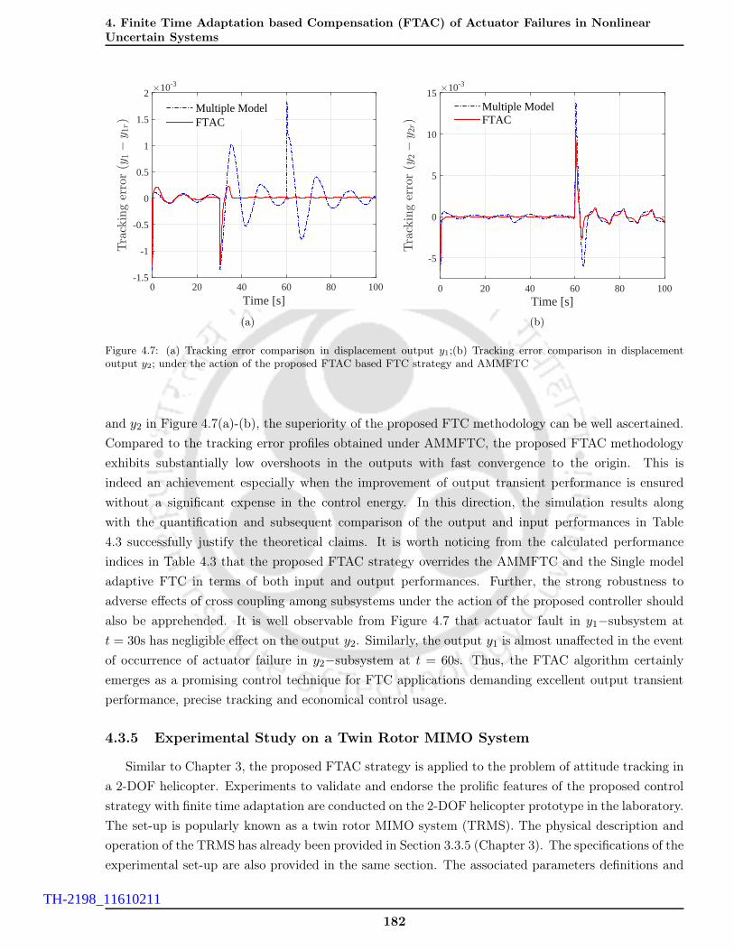
4. Finite Time Adaptation based Compensation (FTAC) of Actuator Failures in NonlinearUncertain Systems
Time [s]0 20 40 60 80 100
Trackingerror(y
1−y1r)
×10-3
-1.5
-1
-0.5
0
0.5
1
1.5
2
Multiple ModelFTAC
(a)
Time [s]0 20 40 60 80 100
Trackingerror(y
2−y2r)
×10-3
-5
0
5
10
15Multiple ModelFTAC
(b)
Figure 4.7: (a) Tracking error comparison in displacement output y1;(b) Tracking error comparison in displacementoutput y2; under the action of the proposed FTAC based FTC strategy and AMMFTC
and y2 in Figure 4.7(a)-(b), the superiority of the proposed FTC methodology can be well ascertained.
Compared to the tracking error profiles obtained under AMMFTC, the proposed FTAC methodology
exhibits substantially low overshoots in the outputs with fast convergence to the origin. This is
indeed an achievement especially when the improvement of output transient performance is ensured
without a significant expense in the control energy. In this direction, the simulation results along
with the quantification and subsequent comparison of the output and input performances in Table
4.3 successfully justify the theoretical claims. It is worth noticing from the calculated performance
indices in Table 4.3 that the proposed FTAC strategy overrides the AMMFTC and the Single model
adaptive FTC in terms of both input and output performances. Further, the strong robustness to
adverse effects of cross coupling among subsystems under the action of the proposed controller should
also be apprehended. It is well observable from Figure 4.7 that actuator fault in y1−subsystem at
t = 30s has negligible effect on the output y2. Similarly, the output y1 is almost unaffected in the event
of occurrence of actuator failure in y2−subsystem at t = 60s. Thus, the FTAC algorithm certainly
emerges as a promising control technique for FTC applications demanding excellent output transient
performance, precise tracking and economical control usage.
4.3.5 Experimental Study on a Twin Rotor MIMO System
Similar to Chapter 3, the proposed FTAC strategy is applied to the problem of attitude tracking in
a 2-DOF helicopter. Experiments to validate and endorse the prolific features of the proposed control
strategy with finite time adaptation are conducted on the 2-DOF helicopter prototype in the laboratory.
The set-up is popularly known as a twin rotor MIMO system (TRMS). The physical description and
operation of the TRMS has already been provided in Section 3.3.5 (Chapter 3). The specifications of the
experimental set-up are also provided in the same section. The associated parameters definitions and
182
TH-2198_11610211

4.3 Finite Time Adaptation based Compensation (FTAC) of Actuator Failures inMulti-Input-Multi-Output (MIMO) Nonlinear Uncertain Systems
Time [s]0 20 40 60 80 100
Displacementy1=
x1,1
-0.3
-0.2
-0.1
0
0.1
0.2
0.3
0.4
0.5
y1y1r
(a)
Time [s]0 20 40 60 80 100
Displacementy2=
x2,1
-0.6
-0.4
-0.2
0
0.2
0.4
0.6
0.8
1
y2y2r
(b)
Time [s]0 20 40 60 80 100
Con
trol
inputs
-1.5
-1
-0.5
0
0.5
1
1.5
2u1
u2
(c)
Time [s]0 20 40 60 80 100
Con
trol
inpu
ts
-1.5
-1
-0.5
0
0.5
1
1.5
2
2.5
u1
u2
(d)
Figure 4.8: (a) Time evolution of y1(t) under the proposed adaptive FTC using FTAC;(b) Time evolution of y2(t) underthe proposed adaptive FTC using FTAC;(c) Control inputs u1 and u2 under the proposed FTC scheme using FTAC; (d)Control inputs u1 and u2 under AMMFTC.
Table 4.3: Tabular comparison of output and input performances under proposed FTC under finite time adaptationbased control (FTAC), AMMFTC and adaptive FTC using a single identification model
Control SchemesOutput Performance metrics Input Performance metrics
ITAE RMSE Control Energy Total Variation
y1 y2 y1 y2 u1 u2 u1 u2
FTAC 0.1205 1.8399 0.00012 0.00094 285.58 637.35 14.67 29.22Multiple Models 1.1727 3.5234 0.00036 0.0015 285.26 637.09 14.85 29.04Single Model 13.01 116.66 0.0028 0.0231 285.26 573.73 14.20 27.04
183
TH-2198_11610211

4. Finite Time Adaptation based Compensation (FTAC) of Actuator Failures in NonlinearUncertain Systems
their nominal values appear in Table 3.4. Further the detailed dynamical modeling and parametrization
in terms of unknown system parameters for the TRMS is discussed in Section 3.3.5 in equations (3.219)
through (3.227). To ensure completeness, the dynamical model of the TRMS reiterated along with
the formulation of the parametric model for parameter estimation. The dynamical description of the
nonlinear coupled twin rotor MIMO system is as follows (please refer to Section 3.3.5 for details).
x1 = x2
x3 = x4
x2 = θ∗1x52 + θ∗2x5 − θ∗3 sinx1 − θ∗4x2 + θ∗5x4
2 sin(2x2)
−θ∗6x4x52 cos(x1) − θ∗7x4x5 cos(x1)
x4 = θ∗8x62 + θ∗9x6 − θ∗10x4 − θ∗11x5
2 − θ∗12x5
x5 = −θ∗13x5 + θ∗14uvx6 = −θ∗15x6 + θ∗16uhy1 = x1, y2 = x3
(4.178)
The outputs of the TRMS are pitch and yaw angles and are denoted by y1 and y2. The unknown
parameter vector is defined as θ∗ := [θ∗1, θ∗2, . . . , θ
∗14, θ
∗15, θ
∗16]
T . The definition of all the unknown
parameters θi for i = 1, . . . , 14 are as follows.
θ∗1 = a1/Iv; θ∗2 = b1/Iv; θ
∗3 = Mg/Iv; θ
∗4 = B1αv/Iv; θ
∗5 = 0.0326/2Iv ; θ
∗6 = kgya1/Iv ;
θ∗7 = kgyb1/Iv; θ∗8 = a2/Ih; θ
∗9 = b2/Ih; θ
∗10 = B1αh
/Ih; θ∗11 = −1.75kca1/Ih;
θ∗12 = −1.75kcb1/Ih; θ∗13 = T10/T11; θ
∗14 = km/T11; θ
∗15 = T20/T21; θ
∗16 = kt/T21
(4.179)
Further, the parametric model for unknown parameter estimation is formulated as,
x =
x1
x3
x2
x4
x5
x6
=
x2
x4
0
0
0
0
+
01×7 01×5 01×2 01×2
01×7 01×5 01×2 01×2
ϕT1,2 01×5 01×2 01×2
01×7 ϕT2,2 01×2 01×2
01×7 01×5 ϕT1,3 01×2
01×7 01×5 01×2 ϕT2,3
︸ ︷︷ ︸Φ(x,u)
θ∗1θ∗2...
θ∗14θ∗15θ∗16
︸ ︷︷ ︸θ∗
. (4.180)
The regressors are defined as ϕ1,2 := [x25, x5,− sinx1,−x2,−x2
4 sin 2x2,−x4x25 cos x1,−x4x5 cos x1]
T ,
ϕ2,2 := [x26, x6,−x4,−x2
5,−x5]T , ϕ1,3 := [−x5, uv]
T and ϕ2,3 := [−x6, uh]T . The finite time parameter
estimator and the requisite filters are designed using the above estimation model (4.180) and translat-
ing its use to the differential equations in (4.135)-(4.139). At this juncture, prior to control design, it
is assumed that all the states of the system are available for measurement. However, the only states
available for measurement is the pitch angle x1 and yaw angle x3. The remaining states, namely the
pitch rate (x2), the yaw rate (x4), the momenta of the main rotor and tail rotor (Lm and Lt) are un-
available. Therefore, an Extended Kalman Filter (EKF) is designed to estimate the unavailable states
of the TRMS. The details of EKF design are provided in Appendix A.3. The initial conditions of the
184
TH-2198_11610211

4.3 Finite Time Adaptation based Compensation (FTAC) of Actuator Failures inMulti-Input-Multi-Output (MIMO) Nonlinear Uncertain Systems
system are x(0) = [0, 0, 0, 0, 0, 0]T . The EKF states are also initialized at zero. The relative degree
of the pitch (x1) and yaw (x3) subsystems are found to be ℘1 = ℘2 = 3 with respect to the motor
input voltages uv and uh. Hence the controller gains are selected as c1 = [c1,i3i=1]=[15, 2.5, 2.5] and
c2 = [c2,i3i=1]=[10, 2.5, 2]. The damping gains are chosen asc1,2 = c2,2 = g1,3 = g2,3 = 0.3. The pa-
rameters associated with the estimation of θ are chosen as A0 = [diag−14,−14,−16,−16,−14,−14],γ = 2 and K = 1. The adaptive rate matrices are selected as Γ1 = 20I2m+p and Γ2 = 10I2m+p. The
control input voltages uh and uv are maintained within their allowable range of [−2.5, 2.5]V. The ref-
erence trajectories yr,1 and yr,2 to be tracked by the outputs y1 = θv = x1 and y2 = θh = x3 are the
outputs of the reference system Gr(s) =
[diag
0.2
9s2 + 10s + 4,
0.2
9s2 + 10s + 4
]with yd,1 and yd,2 as
the inputs. The inputs to the reference system are yd,1 = 6 + 4 sin(0.05πt) and yd,2 = 12 cos(0.05πt).
Under the action of the proposed FTAC, the TRMS outputs are required to track the outputs of the ref-
erence model Gr(s) to analyze the superior tracking performance over that obtained using AMMFTC.
Further, the tracking efficiency should not be achieved at the cost of excessive control usage. In the
sequel, the experimental results obtained are illustrated and discussed to essentially arrive at certain
conclusions substantiating all theoretical propositions in this chapter.
Given that the command reference inputs are sinusoidal signals defined by yr,1 and yr,2; the TRMS
Time [s](a)
0 10 20 30 40 50 60 70 80 90 100Pitch
angle
θv=
x1(rad)
0
0.2
0.4
0.6
0.8
x1 yr,1
Time [s](b)
)
0 10 20 30 40 50 60 70 80 90 100
Yaw
angle
θh=
x3(rad)
-0.5
0
0.5
x3 yr,2
Figure 4.9: (a) Time evolution of the pitch angle θv = x1 (rad) tracking the reference signal yr,1;(b) Time evolution ofthe yaw angle θh = x3 (rad) tracking the reference signal yr,2.
equipped with the proposed FTAC methodology renders faithful attitude tracking. Besides, the control
185
TH-2198_11610211

4. Finite Time Adaptation based Compensation (FTAC) of Actuator Failures in NonlinearUncertain Systems
Time [s](a)
0 10 20 30 40 50 60 70 80 90 100
Tra
ckin
g er
ror
(rad
)
-0.2
-0.1
0
0.1
0.2
0.3
x1 − yr,1 x3 − yr,2
Time [s](b)
0 10 20 30 40 50 60 70 80 90 100
Con
trol
inpu
ts (
V)
-2
-1
0
1
2
3
Main rotor voltage uv Tail rotor voltage uh
Figure 4.10: (a) pitch and yaw tracking error (rad); (b) control input voltages uv and uh for the main rotor and the tailrotor.
objective is achieved without encroaching the physical limits on the motor armature voltages driving
the horizontal and vertical propellers. The experimental results are depicted in Figures 4.9-4.10. The
proposed control scheme is indeed rewarding in the sense that a precise output tracking is observed in
Figure 4.9. The output tracking error plotted seperately in Figure 4.9 further corroborates the theoret-
ical claims of improved output transient and steady state performance. To elucidate the results further,
the pitch and the yaw angle x1 and x3 exhibit no considerable transients and at steady state, the pitch
and yaw tracking errors oscillate between [−0.015, 0.015] and [−0.05, 0.01], respectively. The maximum
percentage of steady state error is determined with reference to the maximum peak magnitude of the
respective reference signals. The average steady state error in outputs y1 and y2 are approximately
calculated to be 3% and 5%, respectively. Further, Table 4.4 tabulates the calculated performance
measures from experimental results obtained from proposed FTAC and AMMFTC schemes. While
root mean square error (RMSE) and Integral absolute error (IAE) are indices measuring steady state
performance, Integral time absolute error (ITAE) quantifies the transient performance in tracking con-
trol problems. As evident from ITAE values in Table 4.4, the tracking transient performance is almost
at par with AMMFTC in experiments. However, ITAE and RMSE values corresponding to the pro-
posed FTAC strategy indeed hints towards its promising and precise tracking abilities. Moreover, the
input performance tabulations appearing on the same table displays no significant increment in control
usage. Certainly, the transient and steady state performance improvement of the proposed FTAC
186
TH-2198_11610211

4.4 Summary
strategy over AMMFTC is appreciable and noteworthy. These encouraging and promising results ob-
tained through extensive experimentation on a real time system are indeed testaments validating the
theoretical assertions presented in this chapter. In other words, the conclusions drawn from an analysis
of experimental results as mentioned above, acknowledge the conjectural attributes of the proposed
control methodology.
Table 4.4: Tabulation of output and input performances using the proposed FTAC methodology when applied to attitudetracking problem of TRMS.
ControlMethodology
Output Performance Input Performance
RMSE IAE ITAE CE TV
FTACθv 0.011 0.466 22.31 uv 326.68 567.24
θh 0.036 1.645 83.92 uh 145.19 133.37
AMMFTCθv 0.011 1.023 20.56 uv 298.93 217.72
θh 0.032 3.336 84.08 ut 164.10 809.38
4.4 Summary
A new finite time adaptive parameter estimation based backstepping controller is designed to
accommodate finite as well as infinite number of actuator failures in nonlinear systems with large
parametric uncertainties. The boundedness of the closed loop signals using the proposed control scheme
in the case of finite and infinite actuator faults/failures, has been proved through a rigorous stability
analysis. The output transient and steady state performances are improved without significantly
increasing the control usage. Finite time estimation of unknown system parameters and failure induced
parameters is guaranteed. Considering infinite actuator failures, the incorporation of a finite time
parameter estimator into the proposed FE/FTC scheme allows us to define a lower bound on the
minimum transition time T ∗ between two successive actuator failure patterns; in a sense that if T ∗ ≥Ts, the system recovers its nominal performance. Where Ts is the upper bound on the parameter
convergence time. In addition, it is observed that the proposed FTAC method renders reinforced
robustness of estimation towards unknown bounded external disturbances provided its frequency is
higher than the tracking reference signal. By an accurate failure parameter estimation in finite time,
we succeed in achieving a time bound recovery of the nominal exponential tracking performance of
the plant. Different from AMMFTC strategy in Chapter 3 and other FE/FTC schemes with bounded
or at best asymptotic parameter convergence, the proposed control scheme allows the existence of an
explicit upper-bound on the convergence time of the parameter vector comprising of system and failure
parameter estimates. This time is certainly equivalent to the time required by the system to transit
from its faulty state to its nominal state conditions and hence serves as a measure of performance
robustness of the FTC algorithm. Adding to the proficient attributes of the FTAC algorithm discussed
above, it is actually our belief that one of the most important ones which plays an instrumental role
in substantial performance improvement is the efficiency of the adaptation algorithm in terms of both
187
TH-2198_11610211

4. Finite Time Adaptation based Compensation (FTAC) of Actuator Failures in NonlinearUncertain Systems
transient and steady-state behavior. Comparison of simulation results obtained under the proposed
FTAC strategy with those using benchmark adaptive controllers and the one in Chapter 3 further
justifies our conclusion.
Besides, application of the proposed FTAC methodology to coupled nonlinear MIMO systems also
yields promising transient and steady state behavior. Comparison of simulation results obtained using
the benchmark MBSC [6] method , single model adaptive control and AMMFTC methods proposed
in Chapter 3 validates the theoretical claims and unveils the superiority of the proposed FTAC design.
Experimentation on a twin rotor MIMO system also reveal encouraging performance and well justifies
the suitability of the proposed adaptive control method for practical applications.
188
TH-2198_11610211

5Parametrization-free Finite Time
Estimation based Adaptive Compensation
of Actuator Failures in Nonlinear
Uncertain Systems
Contents
5.1 Introduction . . . . . . . . . . . . . . . . . . . . . . . . . . . . . . . . . . . . . 190
5.2 Parametrization-free Finite Time Estimation based Adaptive Compen-
sation of Actuator Failures in Nonlinear uncertain Systems . . . . . . . . . 192
5.3 Summary . . . . . . . . . . . . . . . . . . . . . . . . . . . . . . . . . . . . . . . 214
189
TH-2198_11610211

5. Parametrization-free Finite Time Estimation based Adaptive Compensation of ActuatorFailures in Nonlinear Uncertain Systems
5.1 Introduction
At this juncture, it is evident that active FTC design for nonlinear systems has attracted the
attention of researchers in view of the inherent nature of system dynamics, which is definitely not
linear. In the context of FE based active FTC design, it is indeed apparent from the earlier chap-
ters and the references therein that adaptive control methods have gained immense popularity due
to their simplicity and effectiveness in compensating uncertain actuator faults/failures obviating the
drawbacks and implementation issues in controller reconfiguration/failure prognosis unit. Focussing
on FE based active FTC approaches, direct and indirect adaptive control strategies have been pro-
posed in Chapters 2-4 for MISO and MIMO nonlinear uncertain systems assuming that the actuator
failure induced perturbations are linearly parameterizable. Further, the matched uncertainties in the
nonlinear system due to inaccurate modeling are considered to also exhibit linear parametrization.
In this chapter, a parametrization-free finite time estimation based adaptive FTC built on the basis
of an indirect FE/FTC design architecture is proposed to compensate more general class of actuator
failures. Herein, the perturbations due to actuator failures or faults and matched uncertainties are not
assumed to be linearly parameterized. Further, the lumped uncertainty due to modeling inaccuracies
and fault/failure induced perturbations is considered to be state-dependent and may explicitly or im-
plicitly vary with time. Besides, such an uncertainty is not necessarily assumed to be vanishing. The
proposed FTC methodology is also utilized to compensate intermittent actuator failures in nonlinear
systems considered in this work. Direct adaptive control methods, in large, have been found to be
incapable of compensating infinite actuator failures in nonlinear uncertain systems. However, such
schemes inherently offer a promising output transient performance. Now, infinite actuator failures
induce changes in failure parameters at each instances of such variations while the system paramet-
ric uncertainties remain invariant to the occurrence of such faults/failures. Therefore, we intend to
exploit the strong features of direct adaptive backstepping approach to ensure a rewarding transient
performance in fault free situations while inducting an indirect approach through the use of finite time
adaptive estimator based backstepping control at the last coordinate to counteract infinite actuator
failures. Therefore, a unified adaptive control design has been proposed in this paper to primarily com-
pensate parametrization free infinite actuator failures and maintain closed-loop signal boundedness for
all time. Finite time bound exact estimation of fault induced perturbations and asymptotic output
tracking with improved transients and steady state behavior are additional design objectives to be met.
Adopting such an ideology with exact uncertainty estimation allows us to exactly (not approximately)
recover nominal fault-free transient and steady state performance in the event of faults and failures as
proved later.
Nonetheless, as pointed out in earlier chapters, such an estimator integrated control approach espe-
cially for nonlinear systems pose serious challenges in stability analysis on account of the bidirectional
robustness interaction between the estimator and the controlled system. Such an interaction may
manifest itself in the form of inaccurate estimation adversely affecting output performance. This in-
teraction would be very clear from the stability analysis wherein the salient attributes of the proposed
methodology namely, boundedness of all closed loop trajectories, output performance recovery, asymp-
totic exact output tracking, piecewise exact estimation of system and failure induced uncertainties;
190
TH-2198_11610211

5.1 Introduction
and potential to compensate infinite actuator failures; are proved. Infinite actuator failures result in
discontinuities in failure induced perturbations at time instances wherein the actuator failure pattern
changes and essentially characterizes addition of fast varying non-smooth perturbations to the nonlin-
ear system. Hence rigorous stability analysis of the closed-loop system using the proposed finite time
uncertainty estimator integrated with a backstepping control strategy under infinite actuator failures
for t ∈ [0,∞), is indeed not a trivial task.
Recently, uncertainty estimator/disturbance observer based controller design, popularly known as
ADRC, have attracted considerable interest for control of linear and nonlinear systems [80–83,92, 93].
Further, second order sliding mode based disturbance observation integrated with a suitable controller
has been either proposed for linear or globally Lipschitz nonlinear uncertain systems with globally
Lipschitz lumped uncertainties [139, 140]. Although significant progress has been made, almost all
such methods in literature assume either the unknown uncertainty to be slowly varying or the uncer-
tainties to be globally Lipschitz with precise knowledge of their bounds, which are indeed restrictive
assumptions for practical systems more importantly prone to actuator failures. Although some of the
works [80–83] address FTC of general affine in control non-Lipschitz nonlinear systems, only semi-
global boundedness of trajectories is achieved. In addition, their application to the problem of FTC
in nonlinear systems with uncertainties (not necessarily Lipschitz) with infinite actuator failures, have
not yet been addressed.
Diverting our attention from FTC objectives, within the ambit of ADRC, disturbance observers
inspired from the theory of high gain observers (HGOs) have been proposed in conjunction with a
suitable controller to achieve tracking/stabilization in nonlinear uncertain systems [96, 137]. In order
to circumvent the peaking effect due to high observer gains, such control schemes resort to saturating
the control input beyond a compact region of interest chosen by the designer. This control strategy
is known as globally bounded control (GBC). Nevertheless, the following shortcomings in the context
of theoretical developments in control are of immense motivation in this work. Firstly, at most semi-
global tracking/stabilization is guaranteed. On a second note, although nominal performance recovery
in terms of trajectory convergence and regaining the region of attraction of the nominal system has
been claimed, a crucial design aspect has still remained indiscernible. In fact, to enlarge the region of
attraction as well as to ensure trajectory convergence to their nominal solutions using GBC, simultane-
ous increment in both the saturation limits and observer gains is required [136]. Theoretically, in order
to attain the region of attraction of the nominal system and recover the nominal output performance,
the observer gains must tend to infinity. Now, estimation using high gain disturbance observers are
not robust to measurement noise. With the increase in observer gains, the noise is amplified and hence
the signal to be estimated is lost. It is therefore imperative to design new disturbance observer based
control approaches wherein there exists finite values of observer gains which guarantee exact nominal
output transient and steady state performance recovery along with acceptable stability margins. At
this point, it is clear that the avoidance of peaking phenomenon in such design strategies without
resorting to the concept of GBC would definitely lead to the existence of global stability properties
of closed-loop system trajectories. Hence, the proposed FTC design utilizes a backstepping procedure
augmented with a finite time disturbance estimator and a damping injection at the last coordinate.
191
TH-2198_11610211

5. Parametrization-free Finite Time Estimation based Adaptive Compensation of ActuatorFailures in Nonlinear Uncertain Systems
The incorporation of damping function allows the control design to ensure global stability of closed
loop trajectories [69]. The peaking effect is circumvented by the use of an uncertainty estimator based
on second order sliding modes [132] without the use of saturation. It is shown that there exist fi-
nite values of estimator/observer gains under which the integrated estimator based controller ensures
nominal output performance recovery and restores the region of attraction of the nominal system . In
addition, the disturbance/uncertainty estimator adopted in this work is robust to measurement noise
and does not require the unknown lumped disturbance signal to be slowly varying. The estimation
characterizes exact convergence to the actual time description of the lumped uncertainty (system un-
certainty and failure induced uncertainty) in finite time and does not require any knowledge of the
structure or upper bound of the same. Finally, a detailed and exhaustive stability proof showing the
boundedness of all closed-loop trajectories obtained using the proposed finite time FE integrated FTC
approach under infinitely occuring parametrization-free actuator failures is provided for all t ∈ [0,∞).
Further, asymptotic exact output tracking with exact fault-free transient and steady state performance
recovery is achieved using the proposed FTC scheme in the case of finite occurrence of actuator fail-
ures. Besides, the proposed FTC strategy allows the designer to define a lower bound on the transit
time between two consecutive changes in actuator failure patterns to ensure exact recovery of fault-free
system performance.
In order to investigate the practical applicability, the proposed methodology is evaluated on a non-
linear longitudinal model of large civil aircraft (Boeing 747-100/200) subject to modeling uncertainties
and infinite actuator failures. Simulation results justify theoretical claims and prove the applicability
of the proposed method to the problem of infinite actuator failures in nonlinear systems. The rest
of the chapter is organized as follows. The FTC problem to be solved is formulated and stated in
Section 5.2.2. In Section 5.2.3, the proposed unified adaptive FTC is explained. A detailed closed-loop
stability analysis and output tracking performance are described in Section 5.2.4. In Section 5.2.5, ex-
tensive simulation studies are presented to illustrate the effectiveness in an aircraft control application.
Finally, a summary of this chapter is provided in Section 5.3.
5.2 Parametrization-free Finite Time Estimation based Adaptive Com-
pensation of Actuator Failures in Nonlinear uncertain Systems
5.2.1 Mathematical Notations and Definitions
Due to brevity of presentation, the definitions of terminologies and preliminary notions have dis-
cussed briefly yet in a lucid manner for ease of understanding of the control methodology developed in
the sequel.
• Let us consider a vector ξ(t) ∈ Rn. Then ‖ξ‖p denotes its Lp norm for p ∈ [1,∞) such that
‖ξ‖p :=(∫∞
0 |ξ(s)|pds)1/p
. For p = ∞, the L∞ norm is defined as ‖ξ‖∞ := supt>0|ξ(t)|.
• Defining the family of dilations D(·) as a linear map associated with the weight vector m =
[m1,m2, . . . ,mn]T , by D : (ξ1, ξ2, . . . , ξn) 7→ (m1ξ1,
m2ξ2, . . . ,mnξn), a vector field f :
Rn → R
n is said to be homogeneous with degree ν ∈ R if f(Dξ) = νDf(ξ) ∀ ,mi > 0.
192
TH-2198_11610211

5.2 Parametrization-free Finite Time Estimation based Adaptive Compensation of ActuatorFailures in Nonlinear uncertain Systems
• Let the vector field f(ξ) be homogeneous with degree ν. Therefore, the differential equation
ξ(t) = f(ξ, t) is invariant with respect to the transformation T : (t, ξ) 7→ (−νt,Dξ), implying
homogeneity of solutions, i.e., ξ(t,ξ0) = ξ(−νt, ξ0). Further, the trivial solution ξ = 0 is
globally finite time stable if it is asymptotically stable and ν < 0 [141].
• A set Ω is called dilation-retractable if DΩ ⊂ Ω for all 0 ≤ ≤ 1 [132].
• D(z,κ) ⊆ R℘+p and Dσ ⊆ R
2 denote the region of attraction for the tracking error dynamics and
estimation error variables, respectively. The symbols ℘ defines the relative degree of the system
and the number of unknown parameters κi is given by p.
• Ωǫσ := σ ∈ Dσ : σTPσσ ≤ ǫτε2, ǫ > 1 and Ωǫ
σ ⊂ Dσ; Nσ := σ ∈ Dσ : σTPσσ ≤ τε2 ⊂ Ωǫσ is
a set, arbitrarily small in the direction of σ. The parameter τ > 0 is a design parameter and is
defined later.
• Me := (z, κ) ∈ D(z,κ) : z = 0, F Te κ = 0 is the largest positively invariant set wherein the
tracking error variables finally reside under the action of control.
• M(z,κ) := (z, κ) ∈ D(z,κ) : 12(zTPcz + κTΓ−1κ) ≤ c, c > 0 and Ω(z,κ) ⊂ M(z,κ) denotes the
compact set wherein (z(t0), κ(t0)) are assumed to reside initially.
• λ(M) and λ(M) are meant to denote the maximum and minimum eigen values of a square matrix
M .
5.2.2 Problem Formulation
Let us consider a class of multi input single output nonlinear system affine in control given by,
∑p:
x = f0(x) +p∑i=1
κ∗i fi(x) +m∑j=1
gj(x)uj
y = h(x)
(5.1)
where x := [x1, x2, . . . , xn]T ∈ D ⊆ R
n defines the state vector, y ∈ R is the system output and
uj : [0,∞) → R for j = 1, . . . ,m, denotes the jth control input (output of the jth actuator) whose
actuators may undergo a fault or a failure in course of simultaneous operation over time. The functions
fi(x), gj(x) : D ⊆ Rn → R, for i = 0, . . . , p are smooth nonlinear functions of which the coefficients
κ∗i are assumed to be unknown. The output function h(x) ∈ R is assumed to be a known smooth
function not necessarily nonlinear. The system∑
p can be transformed to a strict feedback form using
a suitable diffeomorphism into a controllable subsystem of order ℘, as given below.
∑c:
ξi = ξi+1 + fi(ξi)Tκ∗, i = 1, ....., ℘ − 1
ξ℘ = a(ξ, η) + f℘(ξ, η)T κ∗ +
m∑j=1
βj(ξ, η)uj
y = ξ1
193
TH-2198_11610211

5. Parametrization-free Finite Time Estimation based Adaptive Compensation of ActuatorFailures in Nonlinear Uncertain Systems
where, ξi := [ξ1, ξ2, . . . , ξi]T , fi(ξi) := [Lifk
h(x)pk=1]T for i = 1, ℘, a(ξ, η) := L℘f0h(x) and βj(ξ, η) :=
LgjL℘−1f0
h(x). Further, the subsystem∑
z : η = Λ0(ξ, η) +∑p
i=1 κ∗iΛi(ξ, η), η ∈ R
n−℘ is input-to-
state(ISS) stable with respect to ξ as its input.
Hereafter, we assume that the actuators in the system may experience a malfunctioning character-
ized by partial loss of effectiveness (PLOE) fault or actuator lock-in-place (LIP) failures. The in-
put/output(i/o) characteristics of such faults and failures for t ∈ [toj,h, tej,h), h ∈ Z+, can be modeled
as [6]:
uj(t) =
Kj,huHj + uFj,hφj,h, t ∈ [toj,h, t
ej,h)
uHj, t ∈ [tej,h, toj,h+1)
(5.2)
where h = 1, . . . ,∞ and Kj,h ∈ [0, 1] represents the health factor of the jth actuator at the hth
instant of the fault incurred. The terms uHj and uj denote the controller output fed as input to the
jth actuator and the output of the jth actuator respectively. The function φj,h(·) denotes the basis
function depending on which the partial, stuck, and oscillatory failures are characterized by the fault
model in (5.2). In LIP/oscillatory failures, the magnitude at which the jth actuator is stuck/amplitude
of oscillations is given by uFj with φj,h = 1 or any piecewise continuous bounded function of time while
φj,h = 0 features partial loss. The time variables toj,h and tej,h denote the time instants at which hth
failure of the jth actuator starts and ends, respectively. The jth actuator remains healthy for the time
interval t ∈ [tej,h, toj,h+1) until the onset of the (h + 1)th failure at t = toj,h+1. Further, in contrast to
the earlier works in [17,31,32], the basis function φj,h(·) is assumed to be unknown with each actuator
undergoing a transition from its normal mode of operation to various failure modes, infinitely many
times. In addition, the transit time T ∗ between the occurrence of two consecutive actuator failure
patterns is nonzero and finite. It is worth mentioning that the failure model (5.2) can be used to
characterize the i/o behavior of a healthy actuator(kj,h = 1, uFj,h = 0) as well. Hence, in order to
proceed with controller design, the failure model (5.2) can be incorporated into the controllable plant
dynamics∑
p irrespective of the actuators being healthy or affected by faults.
Assumption 5.1. The plant∑
p under the action of a suitably designed failure compensation scheme
can at most tolerate up to (m − 1) actuator failures at any particular instant of time. This ensures
that the plant is associated with atleast one control input ∀t > 0 corresponding to any actuator failure
pattern, to guarantee the existence of stable solutions. The actuator failures are assumed to be unknown
in time, pattern and magnitude.
Assumption 5.2. The reference trajectory to be tracked by the output of the plant∑
p is the output of
a stable linear reference model described as [yd(t)] = Gr(s)[yr(t)]. Where Gr(s) = km/(s℘+a℘−1s
℘−1+
. . .+a1s+a0) and yr(t) being bounded and piecewise continuous. Therefore, the signals (yd, yd, . . . , y(℘)d )
are continuous, bounded and hence belong to a compact set.
Having stated the preliminary assumptions, the problem lies in the design of an active fault tol-
erant controller aimed at achieving closed loop signal boundedness with asymptotic output tracking
irrespective of finite and infinite actuator failures. In addition, attaining nominal transient performance
recovery while being afflicted by such faults is another prime concern. With contextual reference to
194
TH-2198_11610211
5.2 Parametrization-free Finite Time Estimation based Adaptive Compensation of ActuatorFailures in Nonlinear uncertain Systems
FTC, apart from design of controllers rendering asymptotic stability, schemes ensuring the latter fol-
lowed by proof of nominal transient performance recovery has not been addressed so far in literature.
In the section that follows, we shall look into the challenges involved in adaptive control design to
compensate possible infinite actuator failures. Accordingly, we shall come up with a unified optimal
solution which would deliver to the design objectives while adhering to the basic assumptions in control
synthesis.
5.2.3 Proposed Adaptive FTC Design for Infinite Actuator Failures
Considering βjuHj = u0 for j = 1, . . . ,m and the fault model (5.2), the plant dynamics at the ℘th
step exhibit two different forms corresponding to fault free and fault affected scenarios. Let us define
the index set of actuators as B = j1, j2, . . . , jm. Thereafter, two subsets BhtotF
:= j1, j2, . . . , jkhand Bh
parH:= B \ Bh
totFcorrespond to the index set for each of the possible/compensable failure
patterns and loss of effectiveness faults encountered at the hth instant, respectively. Encompassing
both the forms, the unified model for control design is represented as,
ξi = ξi+1 + fi(ξi)Tκ∗ i = 1, . . . , ℘− 1
ξ℘ = f0(ξ, η) + f℘(ξ, η)T κ∗ + gu0 + βTuφ (5.3)
with the terminologies defined as, β = [βjmj=1]T ; g :=
∑j∈Bh
parHKj,h, uφ := [uj,hmj=1]
T with
uj,h = 0 with j 6∈ BhtotF
for cases of actuator failures while g := m, uφ := 0m×1 define a no fault
scenario. At this juncture, it is suitable to assume that uncertainties induced due to feasibly infinite
actuator faults are piecewise continuous and differentiable.
5.2.3.1 Controller Design
System parametric uncertainties due to modeling imperfections are invariant to changes in actuator
failure pattern. Assuming the knowledge of full state vector, the controller is designed following a tuning
function based backstepping until the (℘ − 1)th step finally followed by a finite time exact adaptive
estimator based feedback control at the ℘th step to arrive at the actual control input u0. The motivation
behind the development of such a unified adaptive scheme has been discussed in the introduction.
Proceeding with the control design, let us define the error variables as, zi = ξi−αi−1−y(i−1)d , i = 1, ℘.
The stabilizing control law αi for each of the ith error subsystem are,
αi = −cizi − ci|ψi|2zi − zi−1 − ψTi κ−i−2∑
k=1
zk+1∂αk∂κ
Γψi
− ∂αi−1
∂κΓψi +
(i−1∑
k=1
∂αi−1
∂ξkξk+1 +
i−1∑
k=0
∂αi−1
∂y(k)d
yk+1d
)(5.4)
˙κ = −Γω℘−1, ω℘−1 = ω℘−2 + ω℘−1z℘−1 (5.5)
ψi = fi(ξi) −i−1∑
k=1
∂αi−1
∂ξkfk(ξk) (5.6)
195
TH-2198_11610211

5. Parametrization-free Finite Time Estimation based Adaptive Compensation of ActuatorFailures in Nonlinear Uncertain Systems
Thereafter, the actual control input u0 is finally derived following a backstepping technique integrated
with a finite time exact estimator module to estimate system uncertainties and the intruding pertur-
bations due to faults/failures. The expression for u0 is derived as,
u0 = (−z℘−1 − (c℘ + s℘)z℘ − f0(ξ, η) − ∆℘ + y(℘)d )/m (5.7)
wherein, s℘ = c℘
∣∣∣∣√
∆2℘ + ς
∣∣∣∣, ci, ci,Γ > 0 denote the controller design parameters; κ and ∆℘ are
notations meant to represent estimates of κ∗ and stacked static and dynamic uncertainties ∆∗℘ incurred
due to modeling inaccuracies and actuator failures, respectively. ∆∗℘ is mathematically defined in the
upcoming sub-section. Nonlinear damping terms have been used in each of the virtual controls and the
actual control law to ensure the input-to-state property of the tracking error dynamics with respect to
κ := κ∗ − κ and ∆℘ := ∆℘ − ∆∗℘ as the inputs.
5.2.3.2 Failure Induced Uncertainty Estimation
As discussed earlier, occurrence of faults and failures in actuators lead to changes in the structure
of system dynamics immediately at the ℘th step. Therefore, the information of the ℘th error variable
z℘ is used to design an adaptive estimator which would render an exact estimate of any uncertainty
irrespective of its nature (static/dynamic/both) in finite time. On the lines of [142], the estimator
is designed as given below. Invoking the dynamics of z℘(t) derived from (5.4) and the fact that a
multiplicative actuator fault can be converted to an additive one [143], the estimator dynamics is as
follows.
˙z℘ = f0(ξ, η) + g0u0 − y(℘)d − k1
√µ⌈z℘ − z℘⌋1/2 + ∆℘
˙∆℘ = −k2µsign(k1
√µ⌈z℘ − z℘⌋1/2sign(z℘ − z℘)) (5.8)
where µ, k1, k2 > 0 constitute the estimator gains, ⌈z℘ − z℘⌋1/2 = |z℘ − z℘|12 sign(z℘ − z℘) and the
uncertainty to be estimated is defined as ∆∗℘ := f℘(ξ, η)
Tκ∗ + α℘−1 +(g−g0)u0 +∑
j∈BhtotF
βj uFj,hφj,h
with g0 = m. The variable ∆℘ gives the exact estimate of ∆∗℘ using the estimator (5.8). The parameters
k1, k2 > 0 are chosen so that the polynomial (s2 + k1s + k2) is Hurwitz. In addition, it is important
to mention that choice of µ > 0 is the deciding factor to achieve exactness and rapidity of estimation
thereby yielding exact asymptotic output tracking. Since faults/failures occur erratically with unknown
degree of severity, a heuristic tuning of µ does not yield a fruitful estimation. Further, re-tuning the
parameter µ at instances depending on the severity of fault incurred, is also infeasible. Hence an
adaptive learning law is formulated to instantaneously estimate an appropriate gain online at the
onset of failures to ensure a faithful estimation of uncertainties. The adaptive learning law is given by,
µ(t) = µ(t0) + γ
∫ t
t0
|z℘(s) − z℘(s)|1/2ds (5.9)
However, prior to providing any insight or basis behind the adaptive law formulation, our primary
aim is to prove boundedness of all closed loop trajectories for a finite µ. A dead-zone function with a
196
TH-2198_11610211

5.2 Parametrization-free Finite Time Estimation based Adaptive Compensation of ActuatorFailures in Nonlinear uncertain Systems
threshold |σ1| < δ has been incorporated into the adaptive law so as to avoid unboundedness of gain
estimation due to noisy measurements in practical scenarios.
5.2.4 Stability Analysis of the Proposed Control System under Infinite Actuator
Failures
In the following, it is first shown that the proposed FE/FTC design approach ensures modularity
between the estimator and the controller. Through the piecewise stability analysis to follow, it is shown
that the proposed FTC strategy satisfies the nonlinear separation principle [69]. In consequence, the
bidirectional robustness interaction between the controller-estimator pair is transformed to a unidirec-
tional interaction from the observer to the controller. In the piecewise analysis below, a piece of time
refers to the time interval between the onset and end of an actuator failure pattern. Within this time
interval, the actuator failure pattern does not change and hence the failure induced uncertainty is also
fixed. It does not exhibit any discontinuity within this time interval.
5.2.4.1 Piecewise Boundedness of Closed-Loop Signals
Considering the system dynamics (5.3), final control input u0(t) in (5.7) and the estimator dynamics
(5.8), we arrive at the closed loop system represented in the following form.
z = Az(z, κ, t)z + Ψκ(z, κ, t)T κ+Bσσ2(·) (5.10)
κ = −ΓΨκz (5.11)
σ1 = −k1√µ|σ1|1/2sign(σ1) + σ2 (5.12)
σ2 = −k2µsign(σ1) − ∆∗℘ (5.13)
The state variables in (5.31)-(5.13) are defined as z := [z1 z2 . . . z℘−1]T ; z := [z z℘]
T ;σ1 = (z℘−z℘), σ2 =
∆℘, σ := [|σ1|1/2sign(σ1) σ2]T . With the definitions si := −ci|ψi|2 and ζik := ∂αi−1
∂κ Γψk, the remaining
terms are described as follows. The matrix Az is given by,
−(c1 + s1) 1 0 · · · 0
−1 −(c2 + s2) · · · ζ2(℘−1) 0
0 −1 − ζ23. . .
. . ....
......
. . .. . . 0
0 −ζ2(℘−1) · · · −(c℘−1 + s℘−1) 1
0 · · · · · · −1 −(c℘ + s℘)
, Bσ = [0 · · · 0 1]T , F (ξ) := [f1(ξ1) f2(ξ2) · · · f℘−1(ξ℘−1)],
ΨTκ :=
1 0 · · · 0
−∂α1∂ξ1
1. . .
......
. . .. . . 0
−∂α℘−2
∂ξ1· · · −∂α℘−2
∂ξ℘−21
0 · · · 0 0
F (ξ)T := W (z, κ)F (ξ)T
197
TH-2198_11610211

5. Parametrization-free Finite Time Estimation based Adaptive Compensation of ActuatorFailures in Nonlinear Uncertain Systems
Figure 5.1: Bidirectional robustness interactions transformed to unidirectional interaction under the proposed FTCstrategy
The bidirectional robustness interaction between the controller-estimator pair is evident from the
closed loop equations in (5.31)-(5.13). As illustrated in Figure 5.1, through the proof of piecewise
boundedness of closed-loop signals in Propositions 5.1-5.3, it is shown that the proposed FTC design
ideology transforms the bidirectional interactions to a unidirectional one which in turn ensures a wide
stability margin.
Therefore, in this spirit, let us consider a Lyapunov function Vz : R℘ × [0,∞) → R = 0.5(zTPcz +
κTΓ−1κ). With Pc = I℘, and in view of no change in system parameters κ due to faults resulting in
˙κ = ˙κ− κ∗ = ˙κ, the first time derivative of Vz yields,
Vz = −zTQz + zTΨTκ κ+ z℘σ2 + κTΓ−1 ˙κ (5.14)
= −℘∑
i=1
ciz2i −
℘−1∑
i=1
ci|ψi|2z2i − c℘|∆℘ + ς| 12 z2
℘ + z℘σ2
≤ −℘−1∑
i=1
ciz2i −
c℘2z2℘ −
[c℘2
+ c℘|∆℘ + ς| 12]|z℘|(|z℘| − ¯σ2)
where ¯σ2 := |σ2|/(0.5c℘ + c℘|∆℘ + ς|1/2). Here, we see that when σ2 term in the numerator grows, the
nonlinear damping term in the denominator also increases correspondingly. Therefore, the effects of
σ2 can be curbed suitably to obtain, |z(t)| ≤ |z(t0)|e−c0t + ‖¯σ2‖∞, with c0 = min1≤i≤℘
ci, c℘/2 which is
known to be the ISS property. Thus, at this point, it is important to state the following remarks.
Remark 5.1. From assumption 2, the reference trajectories and its successive derivatives belong to a
compact set Dyd⊂ Dξ. The set Dξ is also a compact set known as the domain of interest. Defining
a compact set M(z,κ) := (z, κ) ∈ D(z,κ) : 12(zTPcz + κTΓ−1κ) ≤ cz + cκ = c,∃c, cz > 0 ⊂ D(z,κ),
all initial conditions (z(t0), κ(t0)) reside within the compact set Ω(z,κ) ⊂ M(z,κ). In the spirit of semi-
global stability, the set Ω(z,κ) ⊂ M(z,κ), for any finite c, can be made relatively large by suitable choice
of controller gains. Thus, with (z, κ) ∈ M(z,κ), it follows that ξ ∈ Mξ ⊂ Dξ, where ξ ∈ Mξ is also a
compact set.
Remark 5.2. On the other hand, incorporating nonlinear time varying damping into control design
increases the stability and robustness which is indeed rewarding in the following sense. In the event of
occurrence of actuator failures, the damping injection first drives the output trajectories to a bounded
198
TH-2198_11610211

5.2 Parametrization-free Finite Time Estimation based Adaptive Compensation of ActuatorFailures in Nonlinear uncertain Systems
set whose boundaries are defined by ¯σ2 while the proposed estimator allows peaking-free estimation
results without the use of saturation function. Hence these features when unified in the proposed FTC
scheme, solely contribute to the attainment of global stability results. Provided there are no magnitude
and rate constraints on the control signal (which is theoretically sound) and the tracking error dynamics
is certainly input-to-state-stable (ISS) with respect to the uncertainty estimation error; there exists a
control law which ensures globally stable adaptive output tracking.
At this stage, the following proposition is stated which testifies the convergence of tracking error
to its nominal fault/failure-free solutions.
Proposition 5.1. (Boundedness) Under the action of the control law (5.7), ∃ µ > 0, such that
for µ ≥ µ, all trajectories (z, κ, σ) of the closed loop system (5.31)-(5.13) residing initially in the set
Ω(z,κ) × Ωǫσ are bounded for ∀t ≥ 0.
Proof. Proving boundedness of closed loop trajectories require positive invariance of an appropriately
chosen set containing Ω(z,κ) × Ωǫσ and existence of a finite time in which all trajectories starting in
Ω(z,κ) × Ωǫσ enter the chosen set and remain thereafter. It is clear from the expression of Vz in (5.14)
that σ2 = 0 implies the convergence of (z, κ) to the set Me rendering z = 0 asymptotically stable with
a region of attraction D(z,κ). Since Vz(z, κ) is positive definite in D(z,κ) (whose proof is trivial), there
always exists a finite c > max(z,κ)∈Ω(z,κ)
Vz such that M(z,κ) := (z, κ) ∈ D(z,κ) : 12(zTPcz + κTΓ−1κ) ≤
c, c > 0 is a compact subset in D(z,κ) and contains the set of initial conditions Ω(z,κ). In order to
proceed with the analysis, let ε2 = µ−1 and thereafter calculating Vz to be negative definite in the set
S := M(z,κ) × Nσ for ǫ ≤ ǫ1, shall prove the set S to be positively invariant. Therefore in the set,
(z, κ, σ) ∈ Vz(z, κ) = c × Nσ, we have, Vz ≤ −∑℘i=1 ciz
2i + εℓ1 with ℓ1 := max
M(z,κ)
‖∂Vz∂z ‖K1
√τ/λ(Pσ)
and ‖Vz(z, κ, σ2) − Vz(z, κ, 0)‖ ≤ K2K1‖σ‖ in the set S with K2 = maxz∈M(z,κ)
‖∂Vz∂z ‖. Now, in the
set, M(z,κ) × Vσ := σTPσσ = τε2, the following conditions ‖z(z, κ, σ2) − z(z, κ, 0)‖ ≤ K1 and
‖∆℘(z, σ)‖ ≤ K3, are obvious. In this direction, let us call upon the positive definite function Vσ :
Dσ ⊂ R2 \ 0 × [0,∞) → R such that (σ, t) 7→ σTPσσ. Using (5.13), the first time derivative of σ is
given by,
σ =
[12 |σ1|−1/2σ1
σ2
]=
[12 |σ1|−1/2(−k1
ε ⌈σ1⌋12 + σ2)
−k2ε2
sign(σ1) + ∆∗℘(·)
]
= |σ1|−1/2
[−k1
2ε⌈σ1⌋1/2 + σ22
−(k2ε2 − ∆∗℘(·)sign(σ1))⌈σ1⌋1/2
]
= |σ1|−1/2
[−k1
2ε12
−k2ε2
0
]
︸ ︷︷ ︸Aσ
[⌈σ1⌋1/2σ2
]+ ‖∆∗
℘(·)‖
= |σ1|−1/2Aσσ + ‖∆∗℘(·)‖ (5.15)
Therefore, the Vσ can be written as, Vσ ≤ −|σ1|−1/2σT Qσσ+2σTPσ‖∆∗℘(·)‖. The matrix Qσ is positive
199
TH-2198_11610211

5. Parametrization-free Finite Time Estimation based Adaptive Compensation of ActuatorFailures in Nonlinear Uncertain Systems
definite since Aσ is Hurwitz owing to k1, k2, ε > 0. Using the inequality |σ1|12 ≤ ⌈σ1⌋
12 ≤ ‖σ‖ in the
expression for Vσ yields, Vσ ≤ −λ(Qσ)‖σ‖2 + 2σTPσ‖∆∗℘(·)‖. Hereafter, there exists a τ > 0 satisfying
the inequality 2λ2(Pσ)K3 < λ(Pσ)λ(Qσ) and the above conditions, such that Vz ≤ 0 ∀ (z, κ, σ) ∈
Vz = c × Nσ and Vσ ≤ 0 ∀ (z, κ, σ) ∈ M(z,κ) × Vσ = τε2. Finally, from the foregoing arguments
and inequalities, it is proved that the set S is positively invariant.
To proceed next, we shall turn our interest on the σ-dynamics to eventually comment on the behavior
of (z, κ) and prove the second claim. From the proof of positive invariance of S, it is straightforward to
conclude the existence of a finite time with which trajectories residing in the set Ω(z,κ) ×Ωǫσ ultimately
converge to the set S := M(z,κ) ×Nσ. The calculation of this finite time would be shown at the end
of this proof. It is observed that the vector fields ϕ(σ) of the estimation error system (5.12)-(5.13)
are homogeneous with negative degree of homogeneity. With D : (σ1, σ2) 7→ (2σ1,σ2), we get
T : (t, σ) 7→ (−νt,3−iσi), i = 1, 2, satisfying the relation ϕ(Dσ) = −1Dϕ(σ) yielding homo-
geneity degree ν = −1. The negative degree of homogeneity is the key to exact robustness of estimation
towards ∆∗℘ while preserving the properties of homogeneity. Homogeneity of the vector fields in the
proposed estimator contributes to the avoidance of the peaking effect in the proposed FTC [132].
Further, due to homogeneity of solutions (σ1, σ2), Lyapunov function Vσ, the negative definiteness of
Vσ in Nσ ⊂ Ωǫσ is also true in the set Ωǫ
σ (local stability in homogeneous systems implies global
stability). This in turn induces the property of dilation retractability of the set Nσ and hence
Ωǫσ := σ ∈ Dσ : σTPσσ ≤ ǫτε2, ǫ > 1 to the origin. This is illustrated as follows.
Let us consider a ball Nσ ⊂ B0 ⊂ Ω2σ(ǫ = 2) wherein (σ1(t0), σ2(t0)) reside. It is to be noted that the
initial conditions now lie outside the set Nσ. Now consider a sequence of balls obtained by dilation as,
Bi+1 = DBi, 0 < < 1. Asymptotic stability (not exponential) and homogeneity of (σ1, σ2) infers
that every trajectory starting in Bi will enter Bi+1 before a finite time −iνT . Let us consider that T
is the time taken by the trajectories to travel from B0 to B1. The process of retractability of the sets
to the origin is explained as follows. Due to negative definiteness of Vσ, σ ∈ B0 will enter the ball B1,
i.e., σ(T,B0) ∈ B1. Applying dilation on both sides of this immediate expression and using properties
of trajectory invariance due to homogeneity, yields,
D(σ(T,B0)) = σ(−νT,DB0) = σ(−νT,B1) ∈ DB1
with DB1 = B2, i.e., trajectories σ ∈ B1 enter the ball B2 in a finite time −νT . Repeating in the
same manner, it is concluded that the ball Bn(n >> 0) close to the origin is reached from a ball Bi,
in a finite time Ts, represented as sum of a geometric series as,
Ts = −iνT∞∑
i=0
(−ν)i =−iνT
1 −−ν (5.16)
Hence it is proved both through Lyapunov function and homogeneity approach that σ is bounded in
finite time even when it lies initially outside the compact set Nσ.
With the above arguments and (z(t0), κ(t0)) ∈ Ω(z,κ) ⊂ M(z, κ), it is relevant that ‖z(t)−z(t0)‖ ≤ K1t
with K1 > 0(defined at the beginning of the proof) as long as z(t) ∈ M(z,κ). Thus, a finite time T0
independent of ε exists such that ∀ t ∈ [0, T0], (z(t), κ) ∈ M(z,κ). Within this time interval, with a
200
TH-2198_11610211
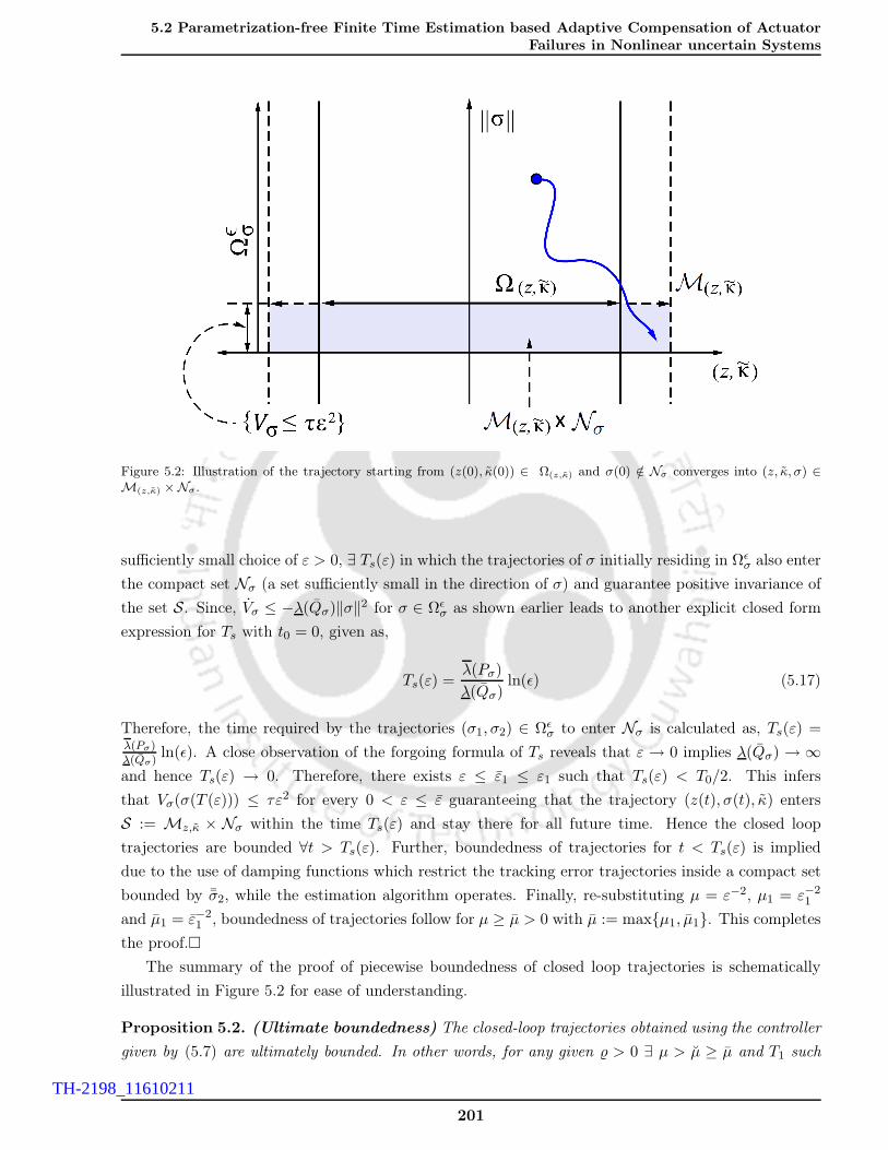
5.2 Parametrization-free Finite Time Estimation based Adaptive Compensation of ActuatorFailures in Nonlinear uncertain Systems
Figure 5.2: Illustration of the trajectory starting from (z(0), κ(0)) ∈ Ω(z,κ) and σ(0) /∈ Nσ converges into (z, κ, σ) ∈M(z,κ) ×Nσ.
sufficiently small choice of ε > 0, ∃ Ts(ε) in which the trajectories of σ initially residing in Ωǫσ also enter
the compact set Nσ (a set sufficiently small in the direction of σ) and guarantee positive invariance of
the set S. Since, Vσ ≤ −λ(Qσ)‖σ‖2 for σ ∈ Ωǫσ as shown earlier leads to another explicit closed form
expression for Ts with t0 = 0, given as,
Ts(ε) =λ(Pσ)
λ(Qσ)ln(ǫ) (5.17)
Therefore, the time required by the trajectories (σ1, σ2) ∈ Ωǫσ to enter Nσ is calculated as, Ts(ε) =
λ(Pσ)λ(Qσ)
ln(ǫ). A close observation of the forgoing formula of Ts reveals that ε → 0 implies λ(Qσ) → ∞and hence Ts(ε) → 0. Therefore, there exists ε ≤ ε1 ≤ ε1 such that Ts(ε) < T0/2. This infers
that Vσ(σ(T (ε))) ≤ τε2 for every 0 < ε ≤ ε guaranteeing that the trajectory (z(t), σ(t), κ) enters
S := Mz,κ × Nσ within the time Ts(ε) and stay there for all future time. Hence the closed loop
trajectories are bounded ∀t > Ts(ε). Further, boundedness of trajectories for t < Ts(ε) is implied
due to the use of damping functions which restrict the tracking error trajectories inside a compact set
bounded by ¯σ2, while the estimation algorithm operates. Finally, re-substituting µ = ε−2, µ1 = ε−21
and µ1 = ε−21 , boundedness of trajectories follow for µ ≥ µ > 0 with µ := maxµ1, µ1. This completes
the proof.
The summary of the proof of piecewise boundedness of closed loop trajectories is schematically
illustrated in Figure 5.2 for ease of understanding.
Proposition 5.2. (Ultimate boundedness) The closed-loop trajectories obtained using the controller
given by (5.7) are ultimately bounded. In other words, for any given > 0 ∃ µ > µ ≥ µ and T1 such
201
TH-2198_11610211

5. Parametrization-free Finite Time Estimation based Adaptive Compensation of ActuatorFailures in Nonlinear Uncertain Systems
that, ‖z(t)‖ + ‖σ(t)‖ ≤ ∀t ≥ T1.
Proof. To prove the above proposition, it is to be shown that trajectories (z, κ, σ) confined in set Sas defined earlier for t > Ts(ε) move towards compact sets nearing the origin. Thereafter, depending
on , the trajectories must enter the corresponding compact set S∗ ⊂ S in a finite time T1 and remain
there forever. In simple words, the set S∗ has to be proved positively invariant.
From Proposition 5.1, it is already proved that all trajectories starting in Ω(z,κ)×Ωǫσ remain in the set S
for all t ≥ Ts(ε). Hence, ∃ µ1 > µ such that for every µ ≥ µ1, the inequality ‖σ(t)‖ ≤ /2 is satisfied for
all t ≥ T1. Now, from the proof of Proposition 5.1, for (z, κ, σ) ∈ S, the Lyapunov function derivative
is given by, Vz ≤ −∑℘i=1 ciz
2i + εℓ1 with ℓ1 := max
M(z,κ)
‖∂Vz∂z ‖K1
√τ/λ(Pσ). Taking
∑℘i=1 ciz
2i ≥ 2εℓ1
assures Vz ≤ −∑℘i=1 ciz
2i /2. Therefore, choosing W(z, κ) := z :
∑℘i=1 ciz
2i ≤ 2εℓ1 as a compact set,
there exists µ ≥ µ2 > µ1 such that the new set S∗ := (z, κ) : Vz ≤ c0, c0 = maxW
Vz(z, κ) ⊂ S and
(z, κ) : Vz ≤ c0 implies ‖z(t)‖ ≤ /2 ∀ t ≥ T1. The above argument proves that all z(t) starting
in S will eventually converge to the set S∗ : (z, κ) : Vz ≤ c0 × Nσ in finite time T1 = max(T1, T1)
considering µ ≥ maxµ1, µ2 ≥ µ. Hence the set S∗ is positively invariant. The claim in Proposition
5.2 follows.
Proposition 5.3. (Nominal Trajectory Convergence) Given > 0, as defined in Proposition 5.2,
∃ µ3 > 0 such that ∀ µ ≥ µ3 > maxµ1, µ2(∀ ε ≤ ε < minε1, ε2; ε2 = µ−1) and (z(t0), κ(t0)) ∈M(z,κ), the solution z(t) and z(t, ε) of the dynamics z(t, z, 0) and the perturbed dynamics z(t, z, σ2)
using the controller in (5.7) ensures ‖z(t, ε) − z(t)‖ ≤ , ∀ t ≥ 0.
Proof. Firstly, it is assumed that the conditions of Proposition 5.1 and 5.2 are satisfied. There-
after, exploiting the property of continuous dependence of solutions of differential equation (5.31)
on initial conditions (i/c) and the estimation error σ2, we invoke Theorem 2 of Chapter 2 in [105],
to infer ∃ > 0 such that for a time Ts(ε) < t = T2 ≤ T1 (T1 has been defined in the previ-
ous proposition), ‖z(T2, ε) − z(T2)‖ ≤ with ‖σ(t)‖ ≤ ; ∀t ≥ T2. Since the trajectories z(t)
satisfy Proposition 5.1, it can be concluded that for t ≤ Ts(ε), ‖z(Ts(ε)) − z(t0)‖ ≤ K1Ts(ε) and
‖z(Ts(ε), ε)− z(t0)‖ ≤ K1Ts(ε). Using these foregoing immediate relations and performing elementary
operations, ‖z(Ts(ε), ε) − z(Ts(ε))‖ ≤ 2K1Ts(ε) is arrived at. Again, using the feature of continuous
dependence of solutions of differential equations on initial conditions (i/c) leads to the inequalities,
‖z(Ts(ε), ε) − z(Ts(ε))‖ ≤ U() with ‖σ(t)‖ ≤ U() ∀ t ≥ T2 and U() > 0. Therefore during the
interval [t0, Ts(ε)] and choosing Ts = U()/2K1, the inequality ‖z(Ts(ε), ε) − z(Ts(ǫ))‖ ≤ U() holds
true. Invoking the aforementioned arguments prove the claim as ‖z(t, ε) − z(t)‖ ≤ , ∀ t ≥ 0.
This property of trajectory convergence is the most amazing property of the proposed control
scheme which can be coined the term performance recovery. Therefore, Propositions 5.1-5.3 hold
under the proposed FTC algorithm and hence fulfills all the conditions required to satisfy nonlinear
separation principle [109]. Finally, modularity between controller and estimator is attained.
202
TH-2198_11610211

5.2 Parametrization-free Finite Time Estimation based Adaptive Compensation of ActuatorFailures in Nonlinear uncertain Systems
5.2.4.2 Further Results on Stability of the Closed-loop System under Infinite Actuator
Failures
In the previous section, Proposition 5.2 states that the closed loop trajectories are ultimately
bounded for µ > µ > µ. These values of gain parameter µ depend on the magnitude of the ultimate
bound. A larger value of µ yields a smaller ultimate bound of the closed loop signals. However, in
the sense of piecewise stability, we are interested in achieving exact asymptotic output tracking which
requires the ultimate bound of σ to be zero. In other words, it is now intended to find an estimator gain
inequality from the estimator dynamics which when satisfied yields an exact estimation with the error
variables converging to zero exactly. Solving the foregoing problem, let us call upon the inequality,
Vσ ≤ −|σ1|−1/2σT Qσσ+2σTPσ‖∆∗℘(·)‖ from the proof of Proposition 5.1. This inequality relation can
be rearranged as Vσ ≤ −|σ1|−1/2σT Qσσ. Where Qσ = −(ATσPσ + PσAσ) and
Aσ :=
[−k1
2ε12
−(k2ε2
− |∆∗℘|)
0
]
Herein, it can be easily figured out that satisfying conditions for asymptotic stability of the origin
(ultimate bound is zero) requires the matrix Aσ to be Hurwitz meaning k2µ > suptoj,h≤t<tej,h|∆∗
℘| =
K3, yielding µ > K3/k2 = µ∗. For k2 = 1 as chosen in the work, µ > suptoj,h≤t<tej,h|∆∗
℘| = µ∗. To
promote notational simplicity, the time interval between the onset and end of a particular actuator
failure pattern defined by [toj,h, tej,h) is replaced by [Th, Th+1) from now onwards. Therefore, from
Proposition 5.2, the following result µ > µ∗ > µ > µ on the choice of µ is derived. In addition, the
estimation error dynamics exhibits negative degree of homogeneity. On account of the same, with the
choice of µ > µ∗, finite time convergence of the estimation error signals is guaranteed. Further as
proved in our works in [144], the estimation error exactly converges to zero in a predefined finite time.
The expression for the upper bound on the convergence time to the origin is Tf defined as follows
Tf (Vσ(0), t0) =2Vσ(0)
K4
where K4 := λ12 (Pσ)λ(Qσ)/λ(Pσ). The detailed calculation is not shown for brevity and instead can
be referred to [144].
Therefore, to this point it is clear that the FTC design scheme until now requires a precise knowledge
of µ∗ to ensure exact estimation of lumped uncertainty and exact asymptotic tracking. However,
since the control problem considers the compensation of actuator failures which are unknown in time,
pattern and magnitude, the knowledge of upper bounds of failure induced uncertainties and their
first derivatives are not available. In Section 5.2.3.2, the motivation behind the design of uncertainty
estimator (5.8) featuring adaptive gains (5.9) has been discussed briefly. Therefore, in this work,
the gain parameters in the proposed uncertainty/disturbance estimator are estimated adaptively and
hence promising performance can be guaranteed in all cases of actuator failures. However, stability
properties of the proposed estimator are yet to be stated and proved. In the following, boundedness
of estimation obtained from the finite time adaptive estimator in the event of infinite actuator failures
203
TH-2198_11610211

5. Parametrization-free Finite Time Estimation based Adaptive Compensation of ActuatorFailures in Nonlinear Uncertain Systems
will be rigorously dealt with. Further, the stability and convergence properties of the tracking error
under the action of the proposed adaptive FTC (5.7) for the case of infinite actuator failures, will be
summarized in the in the form of theorems supported by proofs.
Theorem 5.1. (Piecewise stability properties of the proposed finite time adaptive estima-
tor) Assuming the lumped uncertainty ∆∗℘(·) resulting from modeling imperfections, exogenous dis-
turbances and failure induced uncertainties, to be at least once piecewise continuously differentiable,
the finite time adaptive estimator given by (5.8) with the gain adaptation law in (5.9), ensures finite
time convergence of observer error variables σ1 and σ2 to the origin and yields an exact estimation of
∆∗℘(·). Further, assuming the time interval between two consecutive changes in actuator failure pattern
as [Th, Th+1), h ∈ W, the estimation signals exhibit the following piecewise stability properties, i.e.,
σ1(t) ∈ L1[Th, Th+1) and σ2(t) ∈ L2[Th, Th+1). Here, the index h denotes the occurrence of hth change
in the actuator failure pattern and h = 0 represents initial time.
Proof. Establishing finite time stability of (σ1 = 0, σ2 = 0) necessitates, (1) negative homogeneity
of the vector fields in the estimation error dynamics (5.12)-(5.13); (2) negative definiteness of time
derivative of an appropriately chosen strict Lyapunov function. It has been shown in the proof of
Proposition 5.1 that vector fields in (5.12)-(5.13) possess negative homogeneity of degree ν = −1 < 0.
Thereafter, to prove the second requirement, let us define µ := µ − µ∗ and k1 = k1√µ, k2 = k2µ
for ease of calculation. Thereafter, let us consider a suitably chosen strict Lyapunov function Vσ,h :
R2 \ 0 × R+ × [Th, Th+1) → R+ defined as,
Vσ,h(σ, µ) = µ−32σTPσσ +
2 + 4µ−1µ∗
4γk1µ
−3/2µ2 (5.18)
where Pσ = [pσi,j2i,j=1] is a user defined positive definite symmetric matrix with its elements chosen
as pσ1,1 = 2k2 + k21/2, pσ1,2 = pσ2,1 = −k1/2 and pσ2,2 = 1. These elements pσi,j are selected through
back calculations to ensure that Vσ < 0 and Vσ > 0 [145,146]. Hence to prove stability of the estimator
with forward calculations, let us take the first time derivative of Vσ,h. Using the estimation error
dynamics defined in (5.12)-(5.13) and the adaptive learning law (5.9), the equality obtained is given
by (5.19)-(5.21). Using the conditions to infer negative definiteness of symmetric matrices and given
the fact that k1 = k2 = 1, µ, µ > 0, leads to Vσ,h < −µ−3/2σT Qσµσ ≤ −µ−3/2σT Qσσ < 0, Qσ > 0
proving the piecewise boundedness and finite time stability of the estimation error dynamics, i.e.,
(σ1 = 0, σ2 = 0) is reached in finite time. Further, the immediate inequality of Vσ,h shows that
σ ∈ L2[Th, Th+1) implying that σ1 ∈ L1[Th, Th+1) and σ2 ∈ L2[Th, Th+1).
Having proved the piecewise stability properties of the proposed adaptive uncertainty estimator, the
results are now extended to the time interval t ∈ [0,∞) to prove estimation error boundedness in the
case of infinite actuator failures.
Theorem 5.2. (Extension of piecewise stability properties to t ∈ [0,∞) interval of exis-
tence) From Theorem 5.1, let us consider the stable solutions of the proposed adaptive uncertainty
estimation error dynamics in (5.12)-(5.13) with the adaptive gain learning law (5.9) for the time in-
terval [Th, Th+1), h ∈ W. The following are inferred, (i) In the case of infinitely occurring actuator
204
TH-2198_11610211

5.2 Parametrization-free Finite Time Estimation based Adaptive Compensation of ActuatorFailures in Nonlinear uncertain Systems
failures, the error dynamics of the proposed uncertainty estimator with adaptive gains yields stable
solutions for the time interval [0,∞) which means σ ∈ L∞[0,∞); (ii) In the case of finite actuator
failures, the estimation error signal σ1 is L1 integrable, i.e., σ1 ∈ L1[0,∞).
Proof of (i).
From the proof of Theorem 5.1, the following has already been proved. With the same definition of the
piecewise Lyapunov function in Theorem 5.1 to verify the stability properties of the estimator, from
(5.21) we get Vσ,h ≤ −σT Qσσ. A dead-zone based adaptive tuning law is used to find the estimator
gains. Therefore, invoking the properties of dead-zone based adaptation [110], the estimator gain µ
always converges to a finite limit µ > µ∗. Given µ∗ is a constant, this in turn implies the existence of
a finite bound on µ = µ− µ∗ ≤ ¯µ. Hence the inequality for Vσ,h can be rewritten as
Vσ,h ≤ −µ−3/2σT Qσσ − 1
2γµ2 +
1
2γ¯µ
2(5.22)
The above inequality can be further simplified as
Vσ,h ≤ −ρVσ,h +1
2γ¯µ
2(5.23)
where ρ := minλ(P−1σ )λ(Qσ),
1µ+2µ∗ and Qσ := µ−3/2Qσ. Now let us consider the occurrence
of infinite actuator failures and attempt to utilize the stability properties of the estimator between
[Th, Th+1), (h ∈ Z+) to extend the existence of such stable solutions for all t ∈ [0,∞). Therefore, in this
Vσ,h = µ−3
2 σT Pσσ + µ−3
2 σT Pσσ + µ−3
2 σT Pσσ +(2 + 4µ−1µ∗)k1µµ
µ3
2 γ+
1
2γ
d
dt
(2 + 4µ−1µ∗
2µ3
2
k1
)µ2
= µ−3
2 σT Pσσ −k1
2µ−
3
2 |σ1|−
1
2
((2k2 + k2
1 − 2µ∗)|σ1| −
(k1 −
2
k1
|∆℘|
)|σ1|
)+
1
2γ
d
dt
(2 + 4µ−1µ∗
2µ3
2
k1
)µ2
+1
2γ(2 + 4µ−1µ∗)k1µ
−3
2 µµ −k1
2µ−
3
2 |σ1|−
1
2
(σ2 −
(k1 −
2
k1
|∆℘|
)|σ1|
1
2 sign(σ1)
)2
(5.19)
= µ−3
2 σT Pσσ −k1
2µ−
3
2 |σ1|−
1
2
((2k2 + k2
1 − 2µ∗)|σ1| −
(k1 −
2
k1
µ∗
)2
|σ1| +
(σ2 −
(k1 −
2
k1
µ∗
)|σ1|
1
2 sign(σ1)
)2)
+1
2γ(2 + 4µ−1µ∗)k1µ
−3
2 µµ −1
2γ(µ−2 + 4µ−3µ∗)µµ2
= σT
[−
(2k2+k2
1)
2µ−
3
2 k1µ−2
k1µ−2 − 3
2µ−
5
2
]µσ −
k1
2µ−
3
2 |σ1|−
1
2
((µ − µ∗)(2 + 4µ−1µ∗)|σ1|
)−
1
2γ(µ−2 + 4µ−3µ∗)µµ2
−k1
2µ−
3
2 |σ1|−
1
2
(σ2 −
(k1 −
2
k1µ∗
)|σ1|
1
2 sign(σ1)
)2
+1
2γk1(2 + 4µ−1µ∗)µ−
3
2 (µ − µ∗)µ (5.20)
Using Remainder Theorem, the parameters (k1, k2) are found to satisfy 2k21k2 + 2k2
1 − 4 = 0, and using
the adaptive law from (5.9) as µ = γ|σ1|1/2 > 0 yields,
Vσ,h = µ−3/2σT
[− 3
2µ−1/2
µ−1/2 − 32µ−1
]
︸ ︷︷ ︸Qσ
µσ −k1
2µ−
3
2 |σ1|−
1
2
(σ2 −
(λ1 −
2
λ1µ∗
)2
|σ1|1
2 sign(σ1)
)2
−1
2γ(µ−2 + 4µ−3µ∗)µµ2 < 0
(5.21)
205
TH-2198_11610211

5. Parametrization-free Finite Time Estimation based Adaptive Compensation of ActuatorFailures in Nonlinear Uncertain Systems
direction, a Lyapunov function Vσ : R2 \0×R× [0,∞) → R+ is defined whose piecewise counterpart
defined over the time interval [Th, Th+1) is Vσ,h. In the event of intermittently occurring changes in
the actuator failure patterns affecting the system at time instances Th, (h ∈ Z+), discontinuities are
encountered in the Lyapunov function as well as its value cumulatively increases at every time instance
Th. The magnitude change in the Lyapunov function at the failure instances Th is calculated as,
V (T+h ) − V (T−
h ) ≤ 2 + 4µ−1(T+h )µ∗
4γµ−1(T+
h )µ2(T+h )
− 2 + 4µ−1(T−h )µ∗
4γµ−1(T−
h )µ2(T−h ) (5.24)
V (T+h ) ≤ V (T−
h ) +2 + 4µ−1µ∗
4γµ−1 ¯µ
2 ≤ V (T−h ) + ∆ (5.25)
Here ∆ := 2+4µ−1µ∗
4γ µ−1 ¯µ2
is the maximum magnitude change in the Lyapunov function V (t) at all
failure instances Th and V (T−h ) := lim
t→T−
h
V (t). Further, ∆ is finite due to the usage of dead-zone based
gain adaptation. At this point, using (5.23) and (5.25), the overall system under infinitely varying
actuator failure patterns can be represented as a hybrid system comprising of piecewise continuous
dynamics, discrete dynamics and an impulse sequence Th ∀h ∈ W satisfying 0 ≤ T0 < T1 < T2 <
. . . < Tℵ < T and T → ∞. The notation ℵ is used to denote the total number of changes in the
actuator failure pattern within the time interval [0, T ) ⊃ [Th, Th+1) and ℵ(T0, T ) = (T − T0)/T∗ with
Tℵ < T <∞, T ∗ := minTh+1 − Th for h ∈ W.
Repeating the same procedure as adopted in the proof of Theorem 3.4(i) with the recursive formulations
(5.23) and (5.25) with the choice of T0 = 0 yields,
V (T−) ≤ V (0)e−ρT +¯µ
2
2γρ
(2 − e−ρT
∗
1 − e−ρT ∗
)+
∆
1 − e−ρT ∗ (5.26)
Finally from (5.26), the boundedness of the estimation error σ(t) is proved in the case of infinite
actuator failures, i.e., σ(t) ∈ L∞[0,∞).
Proof of (ii).
Using the inequality ‖σ‖2 ≥ |σ1|1/2 in (5.21) yields the following,
Vσ < −γ|σ1|1/2σT Qσσ ≤ −γλ(Qσ)|σ1| (5.27)
Integrating the above inequality over [Th, Th+1) proves that σ1 ∈ L1[Th, Th+1). Besides the inequality
can be expanded with respect to discrete time instants Th and Th+1 using (5.25) and (5.27) as given
below.
Vσ(T−h+1) ≤ Vσ(T
+h ) − γλ(Qσ)
∫ Th+1
Th
|σ1|dt ≤ Vσ(T−h ) − γλ(Qσ)
∫ Th+1
Th
|σ1|dt + ∆ (5.28)
Utilizing the above inequality (5.28), the following holds for the final time T under ℵ(0, T ) changes in
206
TH-2198_11610211

5.2 Parametrization-free Finite Time Estimation based Adaptive Compensation of ActuatorFailures in Nonlinear uncertain Systems
actuator failure patterns within time [0, T ).
Vσ(T−) ≤ Vσ(T
+ℵ ) − γλ(Qσ)
∫ T
Tℵ
|σ1|dt ≤ Vσ(T−ℵ ) + ∆ − γλ(Qσ)
∫ T
Tℵ
|σ1|dt ≤ . . .
≤ . . . ≤ Vσ(0) + ℵ(0, T )∆ − γλ(Qσ)
∫ T
0|σ1|dt (5.29)
Hence, from (5.29), the L1 bound on σ1 is calculated as follows with T → ∞,
∫ ∞
0|σ1|dt ≤
Vσ(0) + ℵ(0, T )∆
γλ(Qσ)<∞ (5.30)
From (5.30), it is observed that if the occurrence of actuator failures is finite implying ℵ(0,∞) to be
finite, the estimation error signal satisfies σ1 ∈ L1[0,∞).
Now, the final theorem summarizes the stability properties of the proposed adaptive estimator
based backstepping controller to compensate actuator faults and failures followed by the boundedness
of the closed loop trajectories and asymptotic stability of output tracking error dynamics, in the case
of infinite actuator failures.
Theorem 5.3. (Stability of tracking error dynamics for t ∈ [0,∞) interval of existence)
Consider the closed-loop adaptive system consisting of the plant (5.3) affected by actuator faults/failures
modeled in (5.2), the controller (5.7) and the finite time adaptive estimator (5.8) with the adaptive law
(5.9). Under assumptions 5.1-5.2, the following holds. (i) All signals of the closed-loop system are
globally ultimately bounded irrespective of the actuator failures being finite or infinite. (ii) Global
asymptotic stability of the output tracking error dynamics is guaranteed, i.e. limt→∞
z(t) = 0 provided the
occurrence of actuator failures is finite.
Proof of (i).
From Theorem 5.2, the boundedness of σ2 = ∆℘ is guaranteed for all t ∈ [0,∞) in the case of infinite
actuator failures with its piecewise finite time convergence to the origin. Further, the homogeneity
property of the vector fields in the estimation error dynamics (5.12)-(5.13) also restricts the trajectories
to reside within compact sets. With the adaptive learning law for µ starting from an arbitrary small
nonzero initial condition and a suitably chosen adaptive rate γ, the conditions in Proposition 5.1 will
be satisfied. The advantage of this adaptive finite time estimator is its inherent capability to adjust its
gains online and react accordingly to the requirement of the plant so that the trajectories of (z, κ) do
not escape the compact set M(z,κ) for all t > t0 and eventually move towards the origin. A time varying
damping injection contributes to the achievement of global stability results. The adaptive law µ ensures
µ ≥ µ∗ = supTh≤t<Th+1|∆∗
℘| for k1 = k2 = 1. Such a value of µ satisfies both Proposition 5.1 and
5.2 inferring the piecewise ultimate boundedness of closed-loop trajectories. Further, the inequalities
in (5.14) and σ ∈ L∞[0,∞) prove z(t) ∈ L∞[0,∞), z(t) ∈ L∞[0,∞) in the event of infinite actuator
failures.
Proof of (ii).
The ℘-th order tracking error dynamics after substituting the virtual control laws αi defined by (5.4),
207
TH-2198_11610211

5. Parametrization-free Finite Time Estimation based Adaptive Compensation of ActuatorFailures in Nonlinear Uncertain Systems
is reframed in a linear state space form as follows,
z = Az(z, κ, t)z + Ψκ(z, κ, t)T κ+Bσσ2(·) (5.31)
κ = −ΓΨκz (5.32)
The state variables in (5.31) are defined as z := [z1 z2 . . . z℘−1]T ; z := [z z℘]
T ;σ2 = ∆℘. The matrices
Az(z, κ, t), Bσ and Ψκ(z, κ, t)T are defined earlier in the beginning of Section 5.4.3. Let us introduce
an auxiliary state χ(t) := z(t) − N σ1(t) such that N := [0 0 . . . 0 1]T1×℘ and σ1(t) = ⌈z℘ − z℘⌋1/2denoting the estimation error for the state z℘. With this choice of χ, we arrive at a dynamics in χ
driven by σ1 only. Firstly, to deduce such a dynamics from the definition of χ, a more compliant form
of estimation error dynamics is needed so that the theory of Lp spaces can be applied.
In this direction, to begin with the proof, we first invoke the estimation error dynamics in (5.12)-(5.13).
For convenience in analysis, the error dynamics has to be transformed to a more tractable form using
a suitable diffeomorphism. Therefore, using the diffeomorphism σ = [σ1 σ2]T := [⌈σ1⌋1/2 σ2]
T , the
transformed error dynamics is given by,
σ =|σ1|−1/2
2
([−k1 1
−2(k2 − sup∆∗℘) 0
] [σ1
σ2
])(5.33)
Now, let us consider the additional dynamics in (σ1, σ2) as,
σ =
[−k1 1
−2(k2 − sup∆∗℘) 0
][σ1
σ2
](5.34)
Using Filippov’s Theorem 6 of Chapter 2 in [105], it is concluded that the dynamics described in (5.33)
and (5.34) have the same trajectories with identical signal properties if the scaling function |σ1|−1/2
2
is positive definite. With the chosen diffeomorphism and µ > 0, k1 =√µ, k2 = µ for k1 = k2 = 1,
the scaling function satisfies the positive definiteness condition. Hence, the equivalence of solutions
of (5.33) and (5.34) is inferred from Filippov’s Theorem. Thus, from now on the analysis of the the
estimation error will be conducted using the auxiliary error dynamics in (5.34).
The dynamics of χ using the estimation error dynamics (5.34) is described by the following differential
equation.
χ = Az(z, t)χ+ ΨT κ+ N (k1 − (c℘ + s℘))σ1 (5.35)
From Theorem 5.2, the estimation error signal σ ∈ L∞[0,∞) in the event of finite actuator failures.
Therefore, using Hölder’s inequality, it is straightforward to prove that σ1 ∈ L2[0,∞) in the case of
finite actuator failures. It can now be observed that (5.35) is driven by an L2-integrable input σ1.
Therefore, our objective is to prove the L2-integrability of the auxiliary state χ(t). This is due to the
fact that χ(t) ∈ L2[0,∞) implies z(t) ∈ L2[0,∞). Defining χ := [χi℘−1i=1 ]T , χ℘ := z℘ − ⌈σ1(t)⌋1/2,
χ := [χ χ℘]T and proceeding with this aim, we compute,
1d
2dt
(‖χ‖2 + Γ−1‖κ‖2
)≤ χT
(ATz + Az
2
)χ+ χT N σ1
208
TH-2198_11610211
5.2 Parametrization-free Finite Time Estimation based Adaptive Compensation of ActuatorFailures in Nonlinear uncertain Systems
1d
2dt
(‖z‖2 + Γ−1‖κ‖2
)≤ −χTQχ+ χT N σ1 (5.36)
≤ −λ(Q)‖χ‖2 −℘−1∑
i=1
ci|ψi|2χ2i − c℘|∆℘ + ς| 12χ2
℘ + χT N σ1
≤ −λ(Q)‖χ‖2 + χT N σ1 (5.37)
where N := N (k1 − (c℘ + s℘)). Using the Peter-Paul inequality with the factor λ(Q) for the second
term in (5.37) leads to,
χT N σ1 ≤ λ(Q)‖χ‖2
2+
1
2λ(Q)‖N ‖2
∞‖σ1‖2 (5.38)
Substituting (5.38) in (5.37) renders the inequality below,
1
2
d
dt
(‖χ‖2 + Γ−1‖κ‖2
)≤ −λ(Q)
2‖χ‖2 (5.39)
+1
2λ(Q)‖N ‖2
∞‖σ1‖2
The boundedness of N is ensured by taking into account the boundedness of all closed-loop signals un-
der the action of the proposed FTC. Finally, the inequality in (5.39) is re-arranged and then integrated
for the time interval [0,∞) using σ1 ∈ L2[0,∞) which yields,
∫ ∞
0‖χ‖2dt ≤ 1
λ(Q)
(‖χ(0)‖2 + Γ−1‖κ(0)‖2
)
+1
λ(Q)‖N ‖2
∞
∫ ∞
0‖σ1‖2dt ≤ ∞ (5.40)
Given the facts that χ(0) and κ(0) are finite and σ1 ∈ L2[0,∞), the signal property of χ ∈ L2[0,∞) is
easily concluded from (5.40). Therefore, z(t) ∈ L2 follows from the L2-integrability property of χ(t).
Invoking Barbalat’s Lemma, with the signal properties z(t) ∈ L2[0,∞)∩L∞[0,∞) and z(t) ∈ L∞[0,∞)
infers asymptotic stability of the tracking error vector z(t). This completes the proof.
The nominal performance recovery at time Tf and asymptotic convergence of the tracking error
starting from Ω(z,κ) to the origin under the action of the proposed FTC strategy is schematically
illustrated in Figure 5.3.
Further, it can be said that Theorem 5.3 been proved, the proposed controller satisfies the results
in Propositions 5.1 and 5.2. Thereafter, invoking the result in Proposition 5.3, the transient perfor-
mance recovery or the convergence of perturbed system trajectories to those of the nominal system
(assuming known virtual control derivative and free of faults) under adaptive backstepping control is
ensured. Since the estimator gain is adapted online with sufficiently fast adaptive rate γ, the condition
of µ > µ∗ is always satisfied. This choice of estimator gains yields the ultimate bound on (σ1, σ2) to
be zero within a finite time Tf . Hence the proposed design allows to exactly recover the output per-
formance achieved by using a backstepping controller for the nominal system (free from faults/failures).
209
TH-2198_11610211

5. Parametrization-free Finite Time Estimation based Adaptive Compensation of ActuatorFailures in Nonlinear Uncertain Systems
Figure 5.3: Time evolution of z(t) and κ(t) starting in Ω(z,κ) traversing through the set M(z,κ) and ultimately expo-nentially asymptotically converging to origin. The radius k defines the decaying exponential envelope along which z(t)converges to the origin with k → 0 as t → ∞.
Remark 5.3. It should be mentioned that the proposed control scheme can also be used in the case of
the loss of effectiveness fault being state dependent. This is due to the fact that in the proposed adaptive
estimator integrated control scheme, boundedness of all closed loop system trajectories have been proved
by taking into consideration the interaction between the control system and estimator as a consequence
of the interaction between the fault and the system states.
5.2.5 Simulation Studies
In this section, the proposed methodology is applied to compensate infinite number of relatively
frequent PLOE actuator faults and total actuator failures in a nonlinear longitudinal model of a Boeing
747-100/200 aircraft in presence of modeling uncertainties. This study illustrates the effectiveness of
the proposed technique in guaranteeing stability, maintaining nominal fault-free performance (the most
distinctive attribute) while ensuring a faithful and exact disturbance rejection. A Boeing 747-100/200
aircraft longitudinal nonlinear dynamics are considered from [4,111,112] similar to the one considered
in (2.57)-(2.58). The detailed dynamical description along with the definitions and values of the
aerodynamic parameters are referred to Section 2.2.5 in Chapter 2 of this thesis.
210
TH-2198_11610211

5.2 Parametrization-free Finite Time Estimation based Adaptive Compensation of ActuatorFailures in Nonlinear uncertain Systems
Choosing the state variables as [α VT θ q]T = [x1 x2 x3 x4]T = [η ξ]T and using Assumption 5.2,
the system is transformed to a strict feedback form. The elevator deflection angles of the two piece
augmented elevator is δe1=δe2 and are the two actuators u1 and u2. Moreover, the thrust generated by
each engine is chosen to be equal, i.e., Pn1 = Pn2 = Pn3 = Pn4 = Pn. The dynamics in η := [x1 x2]T
describe the internal dynamics of the system with ξ = [x3 x4]T as the input. Input-to-State stability
of the internal dynamics with ξ as the input, was shown in [95]. The transformed system Σc to be
used for controller design is given as,
ξ3 = ξ4, ξ4 = a(ξ, η) + ∆℘(ξ, η) +m∑
j=1
βj(ξ, η)uj (5.41)
where ξ = [ξ3 ξ4]. The infinite actuator faults/failures in both the scenarios are modeled similar to
that in [6] as u1 = uF1,hφ1,h
u2 = (1 −K2,h)uH2
, t ∈ [hT ∗, (h+ 1)T ∗) (5.42)
where h = 1, 3, . . . ,∞. In simulations, the initial state is considered to be [0.0162 230 0.0162 0]T .
Further, the virtual control and actual control parameters are chosen as c1 = 20, c2 = 5, c1 = 0.5, c2 =
0.05, ς = 0.1. The rate parameter in the estimator gain adaptation law is considered as γ = 50. The
reference signal for tracking yd is the output of a reference system as in [66], given by Gr = 1s2+5s+6
and [yd(t)] = Gr(s)[yr(t)] with yr = 0.1 sin(0.5t). The modeling uncertainty ∆a(ξ, η) is additive in
nature and is given by ∆a(ξ, η) = κ∗a(ξ, η), where |κ∗| ≤ 1.
The performance of the proposed methodology is compared with existing FTC scheme by [6] in the
event of infinite actuator failures. The controller proposed by [6] is designed for the system in (5.41),
based on modular backstepping control (MBSC). The notations followed for the control design based
on the methodology of [6] are the same as considered in their work except for the modeling uncertainty
θ which is substituted by the term κ∗ here. For the scheme by [6], it is assumed that |κ∗| ≤ 1 and
0.2 ≤ Kjh ≤ 1 are known at the design phase. The design parameters of the controller by Wang and
Wen [6] are as follows: ζ = 0.05, c1 = 20, c2 = 5, κ2 = 10−6,Γ = 0.5 × I4, ν1 = (0.05 + 2)/2, ν2 = ν3 =
ν4 = 0, σ1 = 1.025 − 0.05, σ3 = σ4 = 10, ς = 0.5 and q = 20.
Fault Scenario 1 : T ∗ = 10s, uF1,h = 5, K2,h = 0.7 and φ1,h = 1, it is observed that the proposed
control scheme and the controller by Wang and Wen [6] yield a faithful output tracking while main-
taining boundedness of all the closed loop signals. The tracking performance along with the control
inputs for both the schemes are shown in Figures 5.4(a)-5.4(f).
Fault Scenario 2 : Here, the failure parameters are assumed to be T ∗ = 10s, uF1,h = 0, K2,h = 0.5
and φ1,h = 1. The output tracking of the desired pitch angle θ and pitch rate q using the pro-
posed controller are illustrated in Figures 5.5(b)-5.5(c) while the tracking performance using both the
methodologies are demonstrated in Figure 5.5(a). The profile of the control inputs u1 and u2 with the
proposed control design and that by [6] are given in Figures 5.5(e)-5.5(f), respectively.
Fault Scenario 3 : This is an extended case which demonstrates the potential of the proposed
scheme in handling oscillatory failures in actuators. For the purpose of illustration of actuator oscilla-
tory failures, the failure parameters are chosen as uF1,h = 2, K2,h = 0.5, φ1,h = sin(2t), T ∗ = 10 and
211
TH-2198_11610211
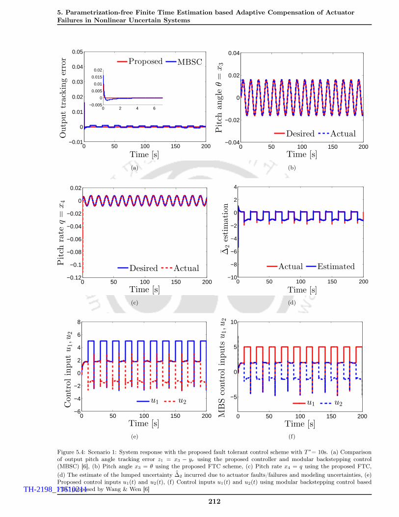
5. Parametrization-free Finite Time Estimation based Adaptive Compensation of ActuatorFailures in Nonlinear Uncertain Systems
0 50 100 150 200−0.01
0
0.01
0.02
0.03
0.04
0.05
Time [s]
Outputtrackingerror
Proposed MBSC
0 2 4 6−0.005
0
0.005
0.01
0.015
0.02
(a)
0 50 100 150 200−0.04
−0.02
0
0.02
0.04
Time [s]
Pitch
angle
θ=
x3
Desired Actual
(b)
0 50 100 150 200−0.12
−0.1
−0.08
−0.06
−0.04
−0.02
0
0.02
Time [s]
Pitch
rate
q=
x4
Desired Actual
(c)
0 50 100 150 200−10
−8
−6
−4
−2
0
2
4
Time [s]
∆2estimation
Actual Estimated
(d)
0 50 100 150 200−6
−4
−2
0
2
4
6
8
Time [s]
Controlinputu1,u
2
u1 u2
(e)
0 50 100 150 200
−5
0
5
10
Time [s]
MBScontrolinputs
u1,u
2
u1 u2
(f)
Figure 5.4: Scenario 1: System response with the proposed fault tolerant control scheme with T ∗= 10s. (a) Comparisonof output pitch angle tracking error z1 = x3 − yr using the proposed controller and modular backstepping control(MBSC) [6], (b) Pitch angle x3 = θ using the proposed FTC scheme, (c) Pitch rate x4 = q using the proposed FTC,
(d) The estimate of the lumped uncertainty ˆ∆2 incurred due to actuator faults/failures and modeling uncertainties, (e)Proposed control inputs u1(t) and u2(t), (f) Control inputs u1(t) and u2(t) using modular backstepping control basedFTC proposed by Wang & Wen [6]
212
TH-2198_11610211

5.2 Parametrization-free Finite Time Estimation based Adaptive Compensation of ActuatorFailures in Nonlinear uncertain Systems
0 50 100 150 200−0.005
0
0.005
0.01
0.015
0.02
Time [s]
Outputtrackingerror
MBSC Proposed
0 2 4 6−0.005
0
0.005
0.01
0.015
0.02
(a)
0 50 100 150 200−0.04
−0.02
0
0.02
0.04
Time [s]
Pitch
angle
θ=
x3
Desired Actual
(b)
0 50 100 150 200−0.12
−0.1
−0.08
−0.06
−0.04
−0.02
0
0.02
0.04
Time [s]
Pitch
rate
q=
x4
Desired Actual
(c)
0 50 100 150 200−4
−2
0
2
4
Time [s]
∆2Estim
ation
Actual Estimated
(d)
0 50 100 150 200
−2
0
2
4
6
8
Time [s]
Controlinputu1,u
2
u1 u2
(e)
0 50 100 150 200
−2
0
2
4
6
8
Time [s]
MBScontrolinputu1,u
2
u1 u2
(f)
Figure 5.5: Scenario 2: System response with the proposed fault tolerant control scheme with T ∗= 10s. (a) Comparisonof output pitch angle tracking error z1 = x3 − yr using the proposed controller and modular backstepping control(MBSC) [6], (b) Pitch angle x3 = θ using the proposed FTC scheme, (c) Pitch rate x4 = q using the proposed FTC,
(d) The estimate of the lumped uncertainty ˆ∆2 incurred due to actuator faults/failures and modeling uncertainties, (e)Proposed control inputs u1(t) and u2(t), (f) Control inputs u1(t) and u2(t) using modular backstepping control basedFTC proposed by Wang & Wen [6]
213
TH-2198_11610211

5. Parametrization-free Finite Time Estimation based Adaptive Compensation of ActuatorFailures in Nonlinear Uncertain Systems
0 50 100 150 200 250−0.04
−0.02
0
0.02
Time [s]
Pitch
angleθ
Desired Actual
(a)
0 50 100 150 200 250−0.1
−0.05
0
0.05
Time [s]
Pitch
rate
q
Desired Actual
(b)
0 50 100 150 200 250−2
0
2
Time [s]∆2estimnation
Actual Estimated
(c)
0 50 100 150 200 250
−5
0
5
10
Time [s]
u1,u
2
u1 u2
(d)
Figure 5.6: Scenario 3: System response with the proposed fault tolerant control scheme. (a) Pitch angle x3 = θ usingthe proposed FTC scheme, (b) Pitch rate x4 = q using the proposed FTC, (c) The estimate of the lumped uncertaintyˆ∆2 incurred due to actuator faults/failures and modeling uncertainties, (d) Proposed control inputs u1(t) and u2(t)
u1 = 2 sin(2t) for 190s ≤ t ≤ 250s. Results appear in Figures 5.6(a)-5.6(d).
Herein, we observe that the proposed scheme is still successful in maintaining the desired nominal
output performance with an acceptable control input. This case had not been considered in the work
in [6] and hence a performance comparison is not drawn.
5.3 Summary
In this chapter, the problem of accommodating infinite number of actuator failures in nonlinear un-
certain systems was addressed. In this context, a new adaptive control scheme was proposed for nonlin-
ear systems affected by infinite failures with inherent modeling uncertainties and matched/mismatched
perturbations. The proposed controller appropriately utilizes direct adaptive backstepping approach to
guarantee an appreciable transient performance in fault free situations and inducts a finite time adap-
tive estimator based control at the last step to counteract infinite actuator failures. The attributes
of the proposed control methodology are boundedness of all closed loop trajectories; output transient
and steady state performance recovery in the event of failures; asymptotic exact output tracking; fi-
nite time exact estimation of system and failure induced uncertainties; and potential to compensate
infinite actuator failures. A rigorous stability analysis of the closed loop system using the proposed
adaptive estimator integrated backstepping controller is conducted to prove stability of the overall
controlled system. Unlike estimators based on HGOs, the adaptive uncertainty estimator does not
induce peaking effect and exact estimation of the lumped uncertainty is achieved with finite values
of estimator gain parameters. These estimator gains are also selected through an adaptive learning
procedure. In addition, the introduction of damping function in the backstepping controller depending
214
TH-2198_11610211

5.3 Summary
on the lumped uncertainty estimation error allows for the existence of global stability of closed-loop
trajectories irrespective of actuator failures being finite or infinite. Consequently, global exponential
asymptotic exact convergence of the output tracking error to the origin is ensured in the event of finite
occurrence of actuator failures without the use of GBC. Different from GBC, the proposed FTC design
methodology also does not require the knowledge of the estimate of the region of attraction which is
required by the former to tune the control saturation level. Besides, for real time applications, unlike
GBC, no trade-off is required to be achieved between the choice of estimator gains for output fault-free
performance recovery and sensitivity of estimation towards measurement noise. In order to study per-
formance of the proposed methodology, it was applied for pitch control in nonlinear longitudinal model
of Boeing 747-100/200 aircraft. Simulation results obtained illustrate the superiority of the proposed
FTC scheme in compensating infinite actuator failures over existing approaches [6, 75, 76] designed
under similar circumstances.
215
TH-2198_11610211

6Conclusions and Scope for Future Work
Contents
6.1 Conclusions . . . . . . . . . . . . . . . . . . . . . . . . . . . . . . . . . . . . . . 217
6.2 Recommendations for Future Research . . . . . . . . . . . . . . . . . . . . . 220
216
TH-2198_11610211

6.1 Conclusions
The research in this thesis is centered around the design, development, analysis and implementation
of adaptive FTC strategies for nonlinear uncertain systems affected by unknown actuator failures.
With the backstepping procedure being central to all the proposed control algorithms, some new
adaptive backstepping algorithms in the context of promising applications to the problem of FTC design
have been proposed. The proposed controllers are aimed at achieving closed loop signal boundedness
asymptotic convergence of the tracking error to the origin with an acceptable transient behavior and
a decent control usage, in the event of unanticipated actuator failures. Besides, the expansion of
their applicability to a large class of dynamical systems is another important design concern. This
thesis is an attempt to address the open issues in adaptive FTC discussed in Chapter 1. An FE/FTC
architecture is adopted to design and investigate all the control algorithms proposed herein. Briefly,
the work done has been summarized below followed by future research recommendations in adaptive
FTC design for nonlinear uncertain systems.
6.1 Conclusions
In Chapter 2, an actuator failure compensation strategy based on direct adaptive control is de-
signed for affine nonlinear uncertain systems affected by faults in the form of partial and total loss of
effectiveness of actuators. The proposed strategy is based on backstepping and adaptive second order
sliding mode control methodologies. The actuator fault/failure induced unknown parameters and the
bounds on system uncertainties are estimated seperately using two adaptive update laws which utilize
the output tracking error information. Asymptotic stability of the output error in nominal scenarios
and in the event of actuator failures is ensured. Improvement of output transient behavior at the
output is shown through a rigorous stability analysis. Compared to ABSC and ASMC based FTC
strategies, the proposed controller reduces the conservatism of the tradeoff between output and input
performance enhancement by rendering an excellent output performance without any increment in
virtual control gains. Further, the cumulative increment of the L∞ bounds on output tracking error
with every instances of actuator failures is eluded. The incorporation of an adaptive second order
sliding mode controller results in a finite time convergence of the last tracking error variable to zero.
In view of the closed loop error analysis under ABSC, the tracking error variable corresponding to the
last coordinate behaves as a disturbance to the remaining reduced closed loop tracking error dynamics.
Further, occurrence of actuator failures directly affects the last error coordinate. Therefore, a finite
time convergence of the last error variable translates to a nominal performance recovery of the reduced
tracking error dynamics both at their transient and steady state phases. Thus , owing to fast and
accurate convergence of the last error variable to the origin, output transient and steady performance
is significantly improved. Such a design attribute also allows us an extra design freedom on defining
a time bound on the nominal performance recovery in the event of actuator faults/failures or occur-
rences of external disturbances. In contrary to the performance recovery in the asymptotic sense, the
nominal performance recovery herein is meant in the finite time sense which means that the actual
output error not only remains close to the nominal trajectory as much is desired but also exhibits a
time bound convergence to the latter, as time elapses. This property is indeed beneficial for FTC ap-
217
TH-2198_11610211

6. Conclusions and Scope for Future Work
plications. Simulation results also confirm that the proposed controller yields enhanced transient and
input performance with no chattering in the control input in comparison with a dedicated ABSC or
relevant ASMC schemes proposed till date in literature. Hence, improvement of transient performance
through the increment of virtual control gains/sliding surface parameters and trajectory initialization
is circumvented. The stability and convergence properties of closed loop signals under the proposed
control law are understood in the global sense.
Thereafter, in Chapter 3, the drawbacks of direct adaptive controllers under an FE/FTC framework,
are discussed and their inability in compensating infinitely time varying failure patterns is mathemati-
cally proved. These shortcomings are circumvented by proposing a new actuator failure compensation
strategy based on indirect adaptive control within the same FE/FTC architecture. Although direct
adaptive strategies have been extensively used for FTC; to the best of author’s knowledge, there are
very few results available in literature which utilize indirect adaptive control to compensate even finite
actuator failures in nonlinear uncertain systems. Such a lack of interest is accrued from the poor output
transient performance obtained using an indirect adaptive scheme during the learning phase. However,
indirect strategies are well known to assure faithful asymptotic tracking/stabilization with an econo-
mized usage of control effort. Therefore, Chapters 3-4 essentially focus on encashing the advantages
of indirect adaptive control while concurrently exploring ways to improve the output transient and
steady state performance without any substantial effect on system stability margins. These chapters
consider the system parametric uncertainty and failure induced perturbations to be linearly param-
eterized. The functions in the regressor matrices associated with unknown parameters are smooth,
not Lipschitz though. Thus, there exists a bidirectional robustness interaction between the certainty
equivalence (CE) controller and the parameter estimator which breaks down the design modularity
and inhibits the existence of global stability of closed loop signals. The region of attraction is de-
creased significantly and any increment in virtual control gains to improve the output performance will
eventually manifest in decremented stability margins, which is undesirable. In Chapter 3, the multiple
model adaptive FTC with two layer adaptation, proposed for the aforementioned nonlinear systems
affected by finite as well as infinite actuator failures, obviates the foregoing design challenges. Multiple
model adaptive estimation based FTC of general nonlinear systems (with linearly parametrized un-
certainties) with transient performance characterization, has not yet been addressed in open literature
even to compensate finite actuator failures. Therefore, contributions in Chapter 3 can be considered
as filling the gap that exists in adaptive backstepping based actuator failure compensation strategies
for nonlinear uncertain systems. The fastness and accuracy of estimation compared to single model
adaptive control parameter estimation are ensured using the two layers of adaptation. As a result, the
output performance of the proposed scheme is promising both at start up and post failure scenarios.
The output transient performance under the proposed adaptive multiple model FTC (AMMFTC) is
quantified and proved to be superior to that obtained using single identification model based adaptive
FTC. Explicit L∞ and L2 bounds on the tracking error for all time t ∈ [0,∞) are derived in the event
of intermittently occurring actuator failures. These bounds provide the designer with an idea of choice
of gains and estimator parameters to improve both input and output transient behavior. The proposed
method exhibits a simpler structure compared to [56] in the sense that a single controller is utilized
218
TH-2198_11610211

6.1 Conclusions
in the design of failure compensation in the event of unknown actuator LOE, LIP float free failures
and intermittent actuator failures. Simulation results illustrate the effectiveness of the proposed FTC
method in the case of infinite actuator faults/failures. The proposed multiple model adaptive control
method has also delivered to the expectations of achieving a fruitful output transient performance
without any substantial increase in control effort.
In Chapter 4, to further enhance output transient performance and to make it more compliant
with practical design requirements, a finite time parameter estimator is inserted within the same
FE/FTC architecture. This ensures finite time exact estimation of the unknown parameters including
those induced by actuator failures and hence a time bound convergence of the output to the nominal
solutions of the healthy system is exhibited. Apart from the above attributes, the finite time adaptation
based controller (FTAC) is also proposed to compensate possible infinite actuator failures. Closed loop
signal boundedness and absolutely integrable property for the output tracking error is established for
all t ∈ [0,∞). The finite time parameter estimation is exact at steady state and additionally robust to
external disturbances. Indeed, Chapter 4 proposes the very first results on finite time estimation based
adaptive FTC to compensate actuator failures. Asymptotic stability of tracking error dynamics, is
guaranteed for finite/infinite number of actuator failures. Nominal performance recovery in the finite
time sense is ensured provided the time between two successive changes in failure patterns is greater
than the convergence time of the estimation error to the origin. The theoretical results obtained are
undoubtedly novel and the algorithm would be a value addition to existing adaptive FTC literature.
Finally, in Chapter 5, the FTC problem is considered for a nonlinear system characterizing linearly
parameterizable and parametrization free modeling uncertainties, affected by finite/infinite actuator
failures. An integrated FE/FTC controller is developed using a backstepping methodology augmented
with an adaptive disturbance observer which estimates total/lumped uncertainty arising due to model-
ing imperfections, external disturbances and actuator failures. Further, a tuning function approach is
used to estimate the mismatched parametric uncertainties until the second last coordinate of backstep-
ping. Following such an approach will avert the dependence on the derivative of parameter estimates
and the closed loop tracking and performance recovery only depend on the total disturbance estima-
tion error at the last coordinate. The modularity of the controller-disturbance pair is established by
incorporating a new time varying damping term into the backstepping controller which decreases the
effect of the disturbance estimation error on the tracking error and ensures its boundedness until the
proposed adaptive disturbance observer estimates the total uncertainty in finite time. The standing
assumption on the lumped uncertainties to be slowly varying with time, is removed. Such an FTC al-
gorithm results in a precise control offering robust transient performance and successful recovery of the
nominal output trajectory(without actuator failures) for the entire time period in the event of abrupt
actuator faults and failures. Compared to existing approaches with similar design features, especially
the most celebrated high gain observer(HGO) based methods, high gain instability due to peaking
is avoided and hence the proposed control methodology also exhibits nominal input performance re-
covery in a finite time sense. The region of attraction corresponding to nominal conditions is also
recovered largely. The avoidance of peaking indeed paves the way for achieving globally stable closed
loop trajectories, global asymptotic stability of output tracking error dynamics and finite time nominal
219
TH-2198_11610211

6. Conclusions and Scope for Future Work
performance recovery. The proposed scheme does not require any knowledge of the bounds of the total
lumped uncertainty introduced into the system at the occurrence of eventualities of faults and fail-
ures.These design attributes have indeed been an unattained goal for a majority of DOB based control
approaches in nonlinear systems which are not globally Lipschitz. The proposed control methodology
is further extended for its application to the FTC problem of accommodating infinite actuator failures
yielding promising and encouraging results. In contrast to bounded or asymptotically stable parame-
ter/uncertainty estimation incurred due to actuator faults, a predefined exact finite time convergence of
the disturbance estimates to their actual temporal profile, allows a lower bound on the minimum time
lapse between two consecutive changes of actuator failure patterns, such that the nominal performance
recovery in the sense of finite time is ensured. Finally, given that the control design is independent
of the structural information of the total uncertainty, it enables the resulting FTC controllers to be
applicable to a wide range of control systems with more general type of actuator failures.
6.2 Recommendations for Future Research
Future possible directions which are worth exploring based on the adaptive FTC algorithms pro-
posed in this thesis are suggested as follows.
• Design and analysis of an adaptive FTC strategy which would not only exhibit finite time es-
timation but also achieve finite time compensation of actuator failures and unknown system
uncertainties.
• Extension of the proposed multiple model adaptive backstepping FTC algorithms to the problem
of compensating actuator failures and nonlinearly parameterized system and failure uncertainties.
• Application of the finite time parameter adaptation algorithm to adaptive control design in
nonlinear uncertain systems with nonlinear parameterizations to improve its performance and
robustness.
• All the adaptive FTC schemes proposed in this thesis assume that all the systems states are
available for measurement. Relaxing this assumption, output feedback design based on the
proposed FTC methodologies is also a research avenue worth exploring.
• Investigating the robustness of the proposed adaptive backstepping FTC methodologies in pres-
ence of input delays and thereafter calculate the time delay margin of such controllers.
• Extension of the proposed design methodologies to the problem of adaptive FTC in time delay
systems.
• Design of optimal adaptive FTC algorithms for uncertain nonlinear systems using dynamic pro-
gramming integrated with the proposed uncertainty estimators.
• Synthesis of adaptive controllers to compensate unknown actuator failures in non-minimum phase
linear and nonlinear systems in presence of modeling uncertainties.
220
TH-2198_11610211

6.2 Recommendations for Future Research
• Experimental validation of the proposed FTC schemes on real time systems such a mobile robot,
quad-copters, axial rotor helicopters and variety of other dynamical systems requiring a self
repairing module.
• Exploring promising possibilities of application of the proposed adaptive strategies to design
controllers operating over a network. The control design would aim to achieve robust stability in
presence of network uncertainties, for instance, limited channel bandwidth, loss of information
packets, communication delay, etc. and also achieve an acceptable output performance.
221
TH-2198_11610211

AAppendix
Contents
A.1 Definition of Performance Indices . . . . . . . . . . . . . . . . . . . . . . . . . 223
A.2 Some Useful Definitions and Inequalities . . . . . . . . . . . . . . . . . . . . 224
A.3 Nonlinear State Estimation: Extended Kalman Filter (EKF) . . . . . . . . 226
A.4 Proof of Lemma 4.1 . . . . . . . . . . . . . . . . . . . . . . . . . . . . . . . . . 228
222
TH-2198_11610211

A.1 Definition of Performance Indices
A.1 Definition of Performance Indices
• The performance indices like peak overshoot (Mp) and peak undershoot (Mu) are used to quantify
the transient performance of the controlled system in regulation and set-point tracking problems.
• For tracking problems wherein the reference trajectory is a smooth time varying and bounded
signal, the transient performance is measured using the integral time absolute error (ITAE).
Whereas, the tracking accuracy (steady state performance) is measured using the integral of the
absolute tracking error (IAE) and root mean square of the error (RMSE). All these performance
metric together constitute the output performance measure of a controlled system. The respective
mathematical definitions of the above stated performance indices are as follows.
ITAE =
T∫
0
t|e(t)|dt (A.1.1)
IAE =
T∫
0
|e(t)|dt (A.1.2)
RMSE =
√√√√√ns∑l=1
e2(l)
ns(A.1.3)
where ns denotes the total number of samples with the time interval [0, T ] with an appropriate
sampling time.
• The control energy (CE) is defined by ‖u‖2 as the 2-norm of the control input and denotes the
input performance. Further, total variation (TV) characterizes smoothness of the control signal
and extent of usage of the control input [113] and is given as
TV =
ns∑
l=1
|ui(l + 1) − ui(l) | (A.1.4)
where ui(1), ui(2), ...., ui(ns) is the discretized sequence of the input signal. A low value of TV
indicates smoothness of the control input.
223
TH-2198_11610211

A. Appendix
A.2 Some Useful Definitions and Inequalities
A.2.1 Definition of Signal Norms and Lp Spaces
• Given, an interval [a, b], the Lp norm of a continuous time vector function f(t) ∈ Rn is defined
as,‖f‖p[a,b] :=
b∫a
‖f(t)‖ppdt =
b∫a
(|f1(t)|p + . . .+ |fn(t)|p)dt
1p
.
• Replacing p = 1, 2,∞, the L1[a, b], L2[a, b] and L∞[a, b] norms are defined as,
‖f‖1[a,b] :=
b∫a
‖f(t)‖1dt, ‖f‖2[a,b] :=
b∫a
‖f(t)‖22dt
12
, ‖f‖∞[a,b] := supt∈[a,b]
max1≤i≤n
‖fi(t)‖
• Given, an interval [a, b], the Lp space is a vector space of functions with a finite Lp norm and
defined as,
Lp[a, b] :=
f ∈ Rn :
b∫
a
‖f(t)‖pp <∞
A.2.2 Signal Convergence Lemmas
Lemma A.1. If f(t), f(t) ∈ L∞ and f(t) ∈ Lp for some p ∈ [1,∞), then f(t) → 0 as t→ ∞.
Proof. Please refer to [122].
Lemma A.2. [Barbălat’s Lemma] If f(t), f(t) ∈ L∞, which means that f(t) is uniformly continuous
and limt→∞
∫ t0 f(s)ds exists and is finite, then f(t) → 0 as t→ ∞.
Proof. Please refer to [122].
A.2.3 Important Inequalities
The following inequalities are immensely useful for adaptive control design and stability analysis.
• Hölder’s Inequality: For p, q ∈ [1,∞] and 1p + 1
q = 1, then f(t) ∈ Lp and g(t) ∈ Lq implies
f(t)g(t) ∈ L1 and ‖f(t)g(t)‖1 ≤ ‖f(t)‖p‖g(t)‖q .
• Peter-Paul Inequality: For p, q ∈ [1,∞] and 1p + 1
q = 1, then f(t) ∈ Lp and g(t) ∈ Lq with
ε > 0 implies ‖f(t)g(t)‖1 ≤‖f(t)‖2
2ε+ε‖g(t)‖2
2, where p = q = 2.
• Minkowski Inequality: For p, q ∈ [1,∞], f(t) ∈ Lp and g(t) ∈ Lp, we have ‖f(t) + g(t)‖p ≤‖f(t)‖p + ‖g(t)‖p implying f(t) + g(t) ∈ Lp.
224
TH-2198_11610211

A.2 Some Useful Definitions and Inequalities
A.2.4 Convex Sets
The following definitions and properties connected to convex sets are referred from [147] and the
detailed proofs can be found therein.
Definition A.1. Let θ1, θ2, . . . , θN be points on a vector space V. Let S be the set of all linear
combinationsN∑i=1
wiθi with wi > 0, i = 1, . . . , N andN∑i=1
wi = 1. The set S is convex.
Figure A.1: Illustration of convex sets
Figure A.1 illustrates the convex sets wherein S2 is convex whereas S1 is not convex. The above
conclusion is drawn from the following property of convex sets which is indeed important for the control
methodology developed in Chapter 3.
Property of Convex Sets: Let θ1, θ2, . . . , θN be points on a vector space V . Any convex set S which
contains θ1, θ2, . . . , θN also contains its linear combinations,∑N
i=1wiθi satisfying wi > 0, i = 1, . . . , N
and∑N
i=1 wi = 1.
Definition A.2. Considering the set S of points θ1, θ2, . . . , θN on a vector space V, the convex hull is
defined as, Conv(S) := N∑i=1
wiθi|∀i : wi > 0 andN∑i=1
wi = 1. A minimum of (n+ 1) points form a
convex hull with a non-empty interior in an n-dimensional vector space.
The concept of convex hull utilized in Chapter 3 to improve the output transient performance is
schematically illustrated in Figure A.2. To obviate the drawbacks of switching, the control design in
Chapter 3 resorts to a second layer of adaptation involving convex combination of parameter estimates
from each of the identification models. In order to ensure a correct parameter estimation, the adaptive
estimates from all the N + 1 identification models must together form a convex hull in the parameter
space containing the actual parameter vector. Thereafter the algorithm is so constructed that the
convex combination of their initial estimates dynamically converges to the actual parameter. Consid-
ering the dimension of actual parameter as N , Figure A.2 shows the convex hull (shaded portion for
225
TH-2198_11610211

A. Appendix
N=2,3) formed by N + 1 parameter estimates from N + 1 identification models in an N−dimensional
parameter space and is seen to contain the actual parameter θ∗ ∈ RN for N=1,2,3.
θ(1)
θ(2)
θ∗
θ(2)θ(3)
θ(1) θ(5)θ(4)
θ∗
θ∗
θ(2)
θ(1)
θ(4)
θ(3)
Figure A.2: Illustration of construction of convex hull in the parameter space for estimating a parameter of dimensionN = 1, 2, 3 (from left to right).
A.3 Nonlinear State Estimation: Extended Kalman Filter (EKF)
A.3.1 Design Motivation
Kalman filter is used to find the best estimate of the unknown states of a dynamical system
from the information available from the measured states in presence of noise [124]. The filter design
primarily relies on the dynamic model of the system acted upon by the control inputs and affected by
noise sources. Briefly, these filters are found useful in (a) extracting information about unmeasurable
quantity from measurable quantity (b) estimating state of a system by combining the series of noisy
measurements available from sensors.
It is obvious from (A.3.1)-(A.3.2) stated below that Kalman filtering is a two step procedure, starting
with the prediction of current state variables, which are then updated once the next measurement is
observed. Since both measurement and estimate may be subjected to some noise with finite covariance,
these estimates are updated using weighted average gain known as the Kalman Gain (K). This Kalman
Gain (K) is determined using the covariances as shown in A.3.2. TO explain the estimation process, let
us consider a continuous-time linear system with the following dynamic and measurement equations:
x = Ax+Bu+ w
y = Cx+ v
w ∼ N (0, Q)
v ∼ N (0, R) (A.3.1)
where x ∈ Rn is the state vector, u ∈ R
m is the control input, y ∈ Rq is the system output and w &
v are zero mean process and measurement noises, respectively. Both the noise signals are assumed to
be Gaussian with covariance Q and R, respectively. The Kalman filter equations used to estimate the
226
TH-2198_11610211

A.3 Nonlinear State Estimation: Extended Kalman Filter (EKF)
state of a system are:
x(0) = E[x(0)]
P (0) = E[(x(0) − x(0))(x(0) − x(0))T ]
K = PCTR−1
˙x = Ax+Bu+K(y − Cx)
P = −PCTR−1CP +AP + PAT +Q (A.3.2)
In first part of the equation, the system model is used to calculate initial state estimate x(0) and initial
noise covariance P (0). The second part of the equation uses these prior estimates and updates them
to find posteriori estimates of the state and noise covariance. This algorithm repeats itself until the
optimal estimate of the state is calculated.
The Kalman filter defined above can be applied to linear systems only. In case of nonlinear systems,
applying Kalman filter directly may not lead to convergence to optimal states. So, the nonlinear system
is first linearized around nominal values which are based on initial guess of system trajectory. The
system whose states represent the deviation of a true state from this nominal state forms an incremental
system which is exactly the linearized system dynamics around the nominal state. Thus, Kalman filter
design methodology can be applied on the linearized system dynamics to estimate the deviation ∆x, and
hence an estimate of true state vector is obtained. However, it is not always straightforward to predict
the nominal state trajectory. In such a case, Extended Kalman Filter (EKF) can be implemented,
which linearizes the nonlinear function around current state estimate obtained from Kalman Filter
itself, and then the resulting Jacobian matrices are used in prediction and updation stages of Kalman
filter algorithm.
A.3.2 Design of Extended Kalman Filter (EKF)
As explained in the preceding text, the design of an EKF seems to follow a ‘bootstrapping proce-
dure’. Let us consider a general non-linear system as follows.
x = f(x, u,w, t)
y = h(x, v)
w ∼ N (0, Q)
v ∼ N (0, R) (A.3.3)
where x ∈ Rn is the state vector, u ∈ R
m is the control input, y ∈ Rq is the system output and w & v are
zero mean process and measurement noises, respectively. The functions f : Rn×R
m×Rn×R+ → R
n
and h : Rn×R
q → Rq are smooth nonlinear and linear functions. Thereafter, using Taylor series, these
227
TH-2198_11610211

A. Appendix
equations (A.3.3) can be linearized around the current state estimate x resulting in:
x = f(x, u0, w0, t) +A∆x+B∆u+ L∆w
y = h(x, v0, t) + C∆x+M∆v (A.3.4)
where the matrices A,B,L,C and M are evaluated at each time step as
A =∂f
∂x
∣∣∣x
B =∂f
∂u
∣∣∣x
L =∂f
∂w
∣∣∣x
C =∂h
∂x
∣∣∣x
M =∂h
∂v
∣∣∣x
(A.3.5)
Assuming that nominal noise values w0 and u0 are zero, the final equations describing the Extended
Kalman Filter (EKF) are
x(0) = E[x(0)]
P (0) = E[(x(0) − x(0))(x(0) − x(0))T ]
˙x = f(x, u0, w0, t) +K(y − h(x, v0, t))
K = PCT R−1
P = AP + PAT + Q− PCT R−1CP (A.3.6)
where Q = LQLT and R = MRMT . Thus using this approach, state estimate, x, of a nonlinear system
(approximated by linearization) is obtained directly. However, for highly nonlinear systems, lineariza-
tion does not provide good approximation, and calculating Jacobians analytically may get complicated.
Moreover, the state transition and measurement model needs to be differentiable for Jacobians to exist.
Otherwise advanced filters need to employed for estimation, which are computationally more expensive
than EKF.
A.4 Proof of Lemma 4.1
Proving that θ∗(t) ∈ S1(ν) is very straightforward. In the worst case, at least one actuator should
be alive to satisfy the controllability condition and ensure the existence of a solution to the FTC
problem. Therefore there exists a lower bound on θ∗1. The lower bound can be derive straightaway as
θ∗1 ≥ minK1b1, . . . ,Kmbm =: ℓ. Further, it can be easily derived from the design assumptions that
parameters jump at time instant Th due to change in the actuator failure pattern. The fault/failure
pattern does not change until the Th+1−th instant of occurrence of the next failure/fault pattern for
h ∈ W. Therefore, if the failure parameter jumps at time t, the following holds.
|θ∗1(t+) − θ∗1(t−)| ≤
m∑
j=1
bj − ℓ (A.4.1)
|θ∗3j(t+) − θ∗3j(t−)| ≤ 2bju (A.4.2)
228
TH-2198_11610211

A.4 Proof of Lemma 4.1
Defining ∆† = maxm∑j=1
bj − ℓ, 2bju < ∞. Now, due to change in actuator faults/failure pattern at
t = Th, the parameter θ∗(t) exhibits a jump whose magnitude is bounded as ‖θ∗(t)‖ ≤ ∆†δ(t− Th).
Therefore, ∀h ∈ W, it is inferred that ‖θ∗(t)‖ ≤ ∆‡∑h
δ(t− Th) with ∆‡ :=√m+ p+ 1∆† (derived
from norm inequalities [110, 122]). The function δ(·) denotes the dirac delta function. At this point,
it is easy to assume that T ≥ T ∗ and t + T ≥ Th+ℵ where, ℵ = T/T ∗ = νT is a positive number.
Hence, the number of changes in the actuator failure pattern between the time t ∼ t + T is ℵ + 1.
Utilizing this immediate assumption along with the assertion and thereafter invoking the properties of
delta functions, the following is obtained,
t+T∫
t
‖θ∗(s)‖ds ≤ ∆‡t+T∫
t
∑
h
δ(s − Th)ds ≤ ∆‡(ℵ + 1) (A.4.3)
The above integral (A.4.3) leads to the property of θ∗(t) stated above, i.e., θ∗(t) ∈ S1(ν). The proof is
complete.
229
TH-2198_11610211

References
[1] J. C. Maxwell, “I. on governors,” Proceedings of the Royal Society of London, vol. 16, pp. 270–283, 1868.
[2] M. T. Hamayun, C. Edwards, and H. Alwi, Fault Tolerant Control Schemes Using Integral Sliding Modes,ser. Studies in Systems, Decision and Control. Switzerland: Springer International Publishing, 2016,vol. 61, no. 1.
[3] “Reconfigurable fault-tolerant control: A tutorial introduction,” European Journal of Control, vol. 14,no. 5, pp. 359 – 386, 2008.
[4] T. Wang, W. Xie, and Y. Zhang, “Sliding mode fault tolerant control dealing with modeling uncertaintiesand actuator faults,” ISA Transactions, vol. 51, no. 3, pp. 386 – 392, 2012.
[5] X. Tang, G. Tao, and S. M. Joshi, “Adaptive actuator failure compensation for parametric strict feedbacksystems and an aircraft application,” Automatica, vol. 39, no. 11, pp. 1975 – 1982, 2003.
[6] W. Wang and C. Wen, “Adaptive compensation for infinite number of actuator failures or faults,” Auto-
matica, vol. 47, no. 10, pp. 2197 – 2210, 2011.
[7] R. Eslinger and P. R. Chandler, “Self-repairing flight control system program overview,” in in Proceedings
of the IEEE National Aerospace and Electron. Conference, Dayton, OH, 1988.
[8] Y. Zhang and J. Jiang, “Bibliographical review on reconfigurable fault-tolerant control systems,” Annual
Reviews in Control, vol. 32, no. 2, pp. 229 – 252, 2008.
[9] X. Yu and J. Jiang, “A survey of fault-tolerant controllers based on safety-related issues,” Annual Reviews
in Control, vol. 39, pp. 46 – 57, 2015.
[10] J. Jiang and X. Yu, “Fault-tolerant control systems: A comparative study between active and passiveapproaches,” Annual Reviews in Control, vol. 36, no. 1, pp. 60 – 72, 2012.
[11] F. Burcham, C. Fullerton, and T. Maine, “Manual manipulation of engine throttles for emergency flightcontrol,” NASA, Technical report NASA/TM-2004-212045, 2004.
[12] K. Ehsan, “Jet airways’ pilot’s act in goa was as miraculous as landing the aircraft on water,” Janta Ka
Reporter, 2016.
[13] “Goa jet airways accident: 15 passengers suffer minor injuries; dgca begins probe,” The Indian Express,2016.
[14] C. Yuan, Y. Zhang, and Z. Liu, “A survey on technologies for automatic forest fire monitoring, detection,and fighting using unmanned aerial vehicles and remote sensing techniques,” Canadian Journal of Forest
Research, vol. 45, no. 7, pp. 783–792, 2015.
230
TH-2198_11610211

References
[15] L. Zhixiang, Y. Chi, Y. Xiang, and Z. Youmin, “Retrofit faultâĂŘtolerant tracking control design ofan unmanned quadrotor helicopter considering actuator dynamics,” International Journal of Robust and
Nonlinear Control, vol. 0, no. 0, 2017.
[16] H. Wu and M. Deng, “Robust adaptive control scheme for uncertain non-linear model reference adaptivecontrol systems with time-varying delays,” IET Control Theory Applications, vol. 9, no. 8, pp. 1181–1189,2015.
[17] G. Tao, S. Joshi, and X. Ma, “Adaptive state feedback and tracking control of systems with actuatorfailures,” IEEE Transactions on Automatic Control, vol. 46, no. 1, pp. 78–95, 2001.
[18] M.-H. Liu and W. Lin, “Multivariable self-tuning control with decoupling robotic manipulators,” IEE
Proceedings D - Control Theory and Applications, vol. 135, no. 1, pp. 43–48, 1988.
[19] H. Alwi and C. Edwards, “Fault tolerant control using sliding modes with on-line control allocation,”Automatica, vol. 44, no. 7, pp. 1859 – 1866, 2008.
[20] M. Hamayun, C. Edwards, and H. Alwi, “A fault tolerant control allocation scheme with output integralsliding modes,” Automatica, vol. 49, no. 6, pp. 1830 – 1837, 2013.
[21] S. S. Tohidi, A. K. Sedigh, and D. Buzorgnia, “Fault tolerant control design using adaptive controlallocation based on the pseudo inverse along the null space,” International Journal of Robust and Nonlinear
Control, pp. n/a–n/a, 2016.
[22] P. S. Maybeck, “Multiple model adaptive algorithms for detecting and compensating sensor and actu-ator/surface failures in aircraft flight control systems,” International Journal of Robust and Nonlinear
Control, vol. 9, no. 14, pp. 1051–1070, 1999.
[23] G. Yen and L.-W. Ho, “Online multiple-model-based fault diagnosis and accommodation,” IEEE Trans-
actions on Industrial Electronics, vol. 50, no. 2, pp. 296–312, April, 2003.
[24] S.-J. Zhang, X.-W. Qiu, B. Jiang, and C.-S. Liu, “Adaptive actuator failure compensation control basedon mmst grouping for a class of mimo nonlinear systems with guaranteed transient performance,” Inter-
national Journal of Control, vol. 88, no. 3, pp. 593–601, 2015.
[25] Y. Yin, P. Shi, and F. Liu, “Gain-scheduled robust fault detection on time-delay stochastic nonlinearsystems,” IEEE Transactions on Industrial Electronics, vol. 58, no. 10, pp. 4908–4916, 2011.
[26] S. Montes de Oca, S. Tornil-Sin, V. Puig, and D. Theilliol, “Fault-tolerant control design using the linearparameter varying approach,” International Journal of Robust and Nonlinear Control, vol. 24, no. 14, pp.1969–1988, 2014.
[27] B. A. Siddiqui, S. El-Ferik, and M. Abdelkader, “Fault tolerant flight control using sliding modes andsubspace identification-based predictive control,” IFAC-PapersOnLine, vol. 49, no. 9, pp. 124 – 129, 2016,6th IFAC Symposium on System Structure and Control SSSC 2016.
[28] Y. Alain, M. Seron, and A. De Doná José, “Robust multiactuator fault-tolerant mpc design for constrainedsystems,” International Journal of Robust and Nonlinear Control, vol. 23, no. 16, pp. 1828–1845, 2012.
[29] Alwi, H. and Edwards, C., “Fault detection and fault-tolerant control of a civil aircraft using a sliding-mode-based scheme,” IEEE Transactions on Control Systems Technology, vol. 16, no. 3, pp. 499 –510,May 2008.
[30] F. Chen, B. Jiang, and G. Tao, “An intelligent self-repairing control for nonlinear MIMO systems viaadaptive sliding mode control technology,” Journal of the Franklin Institute, vol. 351, no. 1, pp. 399 – 411,2014.
231
TH-2198_11610211

References
[31] W. Wang and C. Wen, “Adaptive actuator failure compensation control of uncertain nonlinear systemswith guaranteed transient performance,” Automatica, vol. 46, no. 12, pp. 2082 – 2091, 2010.
[32] X. Tang, G. Tao and S.M. Joshi, “Adaptive actuator failure compensation for nonlinear MIMO systemswith an aircraft control application,” Automatica, vol. 43, no. 11, pp. 1869 – 1883, 2007.
[33] X. Yu and J. Jiang, “Hybrid fault-tolerant flight control system design against partial actuator failures,”IEEE Transactions on Control Systems Technology, vol. 20, no. 4, pp. 871–886, July 2012.
[34] M. Khosrowjerdi, “Mixed H2/H∞ approach to fault-tolerant controller design for lipschitz non-linearsystems,” IET Control Theory & Applications, vol. 5, pp. 299–307, January 2011.
[35] Q. Hu, B. Xiao, and M. Friswell, “Robust fault tolerant control for spacecraft attitude stabilization underactuator faults and bounded disturbance,” Journal of Dynamic Systems, Measurement and Control, vol.133, pp. 051 006–1–051 006–8, 2011.
[36] ——, “Fault tolerant control with H∞ performance for attitude tracking of flexible spacecraft,” IET
Control Theory Applications, vol. 6, no. 10, pp. 1388–1399, 2012.
[37] H. Niemann and J. Stoustrup, “Passive fault tolerant control of a double inverted pendulum: a case study,”Control Engineering Practice, vol. 13, no. 8, pp. 1047 – 1059, 2005.
[38] B. Liang and G. Duan, “Robust H∞ fault-tolerant control for uncertain descriptor systems by dynamicalcompensators,” Journal of Control Theory and Applications, vol. 2, no. 3, pp. 288–292, 2004.
[39] M. Benosman and K.-Y. Lum, “Application of absolute stability theory to robust control against loss ofactuator effectiveness,” IET Control Theory Applications, vol. 3, no. 6, pp. 772–788, 2009.
[40] M. Corradini and G. Orlando, “A sliding mode controller for actuator failure compensation,” in Proceedings
of 42nd IEEE Conference on Decision and Control, vol. 4, Maui, Hawaii, December 2003, pp. 4291–4296.
[41] Corradini, M.L. and Orlando, G. and Parlangeli, G., “Actuator failures compensation: a sliding modecontrol approach,” in 14th Mediterranean Conference on Control and Automation, 2003, pp. 1–6.
[42] Corradini, M.L. and Monteriu, A. and Orlando, G., “An actuator failure tolerant control scheme for anunderwater remotely operated vehicle,” IEEE Transactions on Control Systems Technology, vol. 19, no. 5,pp. 1036–1046, 2011.
[43] M. Hamayun, C. Edwards, and H. Alwi, “Design and analysis of an integral sliding mode fault-tolerantcontrol scheme,” IEEE Transactions on Automatic Control, vol. 57, no. 7, pp. 1783 –1789, July 2012.
[44] ——, “Augmentation scheme for fault-tolerant control using integral sliding modes,” IEEE Transactions
onControl Systems Technology,, vol. 22, no. 1, pp. 307–313, Jan 2014.
[45] P. Baldi, M. Blanke, P. Castaldi, N. Mimmo, and S. Simani, “Adaptive ftc based on control allocation andfault accommodation for satellite reaction wheels,” in 2016 3rd Conference on Control and Fault-Tolerant
Systems (SysTol), Sept 2016, pp. 672–677.
[46] C. Andrea, P. M. M., and J. T. Arne, “Fault-Řtolerant control allocation for overactuated nonlinearsystems,” Asian Journal of Control, vol. 20, no. 2, pp. 621–634.
[47] A. Casavola and E. Garone, “Fault-tolerant adaptive control allocation schemes for overactuated systems,”International Journal of Robust and Nonlinear Control, vol. 20, no. 17, pp. 1958–1980, 2010.
[48] Q. Shen, B. Jiang, P. Shi, and C. C. Lim, “Novel neural networks-based fault tolerant control scheme withfault alarm,” IEEE Transactions on Cybernetics, vol. 44, no. 11, pp. 2190–2201, Nov 2014.
232
TH-2198_11610211
References
[49] J. Han, H. Zhang, Y. Wang, and X. Liu, “Robust state/fault estimation and fault tolerant control for tsfuzzy systems with sensor and actuator faults,” Journal of the Franklin Institute, vol. 353, no. 2, pp. 615– 641, 2016.
[50] X. Zhang, M. M. Polycarpou, and T. Parisini, “Adaptive fault diagnosis and fault-tolerant control of mimononlinear uncertain systems,” International Journal of Control, vol. 83, no. 5, pp. 1054–1080, 2010.
[51] X. Zhang, T. Parisini, and M. M. Polycarpou, “Adaptive fault-tolerant control of nonlinear uncertainsystems: an information-based diagnostic approach,” IEEE Transactions on Automatic Control, vol. 49,no. 8, pp. 1259–1274, Aug 2004.
[52] X. Zhang, M. M. Polycarpou, and T. Parisini, “Fault diagnosis of a class of nonlinear uncertain systemswith lipschitz nonlinearities using adaptive estimation,” Automatica, vol. 46, no. 2, pp. 290 – 299, 2010.
[53] C. Tan, X. Yao, G. Tao, and R. Qi, “A multiple-model based adaptive actuator failure compensationscheme for control of near-space vehicles,” IFAC Proceedings Volumes, vol. 45, no. 20, pp. 594 – 599, 2012,8th IFAC Symposium on Fault Detection, Supervision and Safety of Technical Processes.
[54] X. L. Yao, G. Tao, R. Y. Qi, and B. Jiang, “An adaptive actuator failure compensation scheme for a classof nonlinear mimo systems,” Journal of the Franklin Institute, vol. 350, no. 9, pp. 2423–2441, November2013.
[55] M. A. Yajie, B. Jiang, and G. Tao, “A new multiple-model adaptive actuator failure compensation schemefor a class of nonlinear mimo systems,” in Proceedings of the 34th Chinese Control Conference, vol. 4,July 2015, pp. 6274 –6279.
[56] X. Yao, G. Tao, and B. Jiang, “Adaptive actuator failure compensation for multivariable feedback lin-earizable systems,” International Journal of Robust and Nonlinear Control, vol. 26, no. 2, pp. 252–285,2016.
[57] Q. Yang, S. S. Ge, and Y. Sun, “Adaptive actuator fault tolerant control for uncertain nonlinear systemswith multiple actuators,” Automatica, vol. 60, pp. 92 – 99, 2015.
[58] G. P. Incremona, A. Ferrara, and L. Magni, “Hierarchical model predictive/sliding mode control of non-linear constrained uncertain systems,” IFAC-PapersOnLine, vol. 48, no. 23, pp. 102 – 109, 2015, 5th IFACConference on Nonlinear Model Predictive Control NMPC 2015.
[59] S. E. Boukani, M. J. Khosrowjerdi, and R. Amjadifard, “Terminal sliding mode control allocation fornonlinear systems,” Canadian Journal of Electrical and Computer Engineering, vol. 40, no. 3, pp. 162–170, Summer 2017.
[60] H. Alwi, “Fault tolerant longitudinal aircraft control using non-linear integral sliding mode,” IET Control
Theory Applications, vol. 8, pp. 1803–1814(11), November 2014.
[61] C.-C. Chen and Y.-W. Liang, “Fault tolerant control of nonlinear systems via a ca-based integral slidingmode technique,” in Decision and Control (CDC), 2013 IEEE 52nd Annual Conference on, Dec 2013, pp.19–24.
[62] B. Xu, R. Qi, B. Jiang, and X. Yao, “Nussbaum gain adaptive fault tolerant control for hypersonic vehicleswith uncertain parameters and actuator faults,” IFAC-PapersOnLine, vol. 50, no. 1, pp. 5256 – 5262, 2017,20th IFAC World Congress.
[63] H. Jingjing, Q. Ruiyun, and J. Bin, “Adaptive fault-tolerant control design for hypersonic flight vehiclesbased on feedback linearization,” in Proceedings of the 33rd Chinese Control Conference, July 2014, pp.3197–3202.
233
TH-2198_11610211

References
[64] X. Ma and G. Tao, “Adaptive actuator compensation control with feedback linearization,” IEEE Trans-
actions on Automatic Control, vol. 45, no. 9, pp. 1705–1710, Sep 2000.
[65] J. He, R. Qi, B. Jiang, and J. Qian, “Adaptive output feedback fault-tolerant control design for hypersonicflight vehicles,” Journal of the Franklin Institute, no. 0, pp. –, 2015.
[66] S. Kendrick Amezquita, L. Yan, and W. A. Butt, “Adaptive dynamic surface control for a class of mimononlinear systems with actuator failures,” International Journal of Systems Science, vol. 44, no. 3, pp.479–492, 2013.
[67] S. Kendrick Amezquita, Y. Lin, W. Butt, and C. Y. P. Chen, “Dynamic surface control for a class ofnonlinear feedback linearizable systems with actuator failures,” IEEE Transactions on Neural Networks
and Learning Systems, vol. PP, no. 99, pp. 1–6, June 2016.
[68] S. Sastry, Nonlinear Systems: Analysis, Stability, and Control, ser. Interdisciplinary Applied Mathematics.
[69] M. Krstić, I. Kanellakopoulos, and P. Kokotović, Nonlinear and adaptive control design, ser. Adaptiveand learning systems for signal processing, communications, and control. Wiley, 1995.
[70] D. Swaroop, J. Hedrick, P. Yip, and J. Gerdes, “Dynamic surface control for a class of nonlinear systems,”IEEE Transactions on Automatic Control, vol. 45, no. 10, pp. 1893–1899, Oct 2000.
[71] X. Tang, G. Tao, and S. M. Joshi, “Adaptive output feedback actuator failure compensation for a class ofnon-linear systems,” International Journal of Adaptive Control and Signal Processing, vol. 19, no. 6, pp.419–444, 2005.
[72] Z. Zhang and W. Chen, “Adaptive output feedback control of nonlinear systems with actuator failures,”Information Sciences, vol. 179, no. 24, pp. 4249 – 4260, 2009.
[73] Z. Zhang, S. Xu, Y. Guo, and Y. Chu, “Robust adaptive output-feedback control for a class of non-linear systems with time-varying actuator faults,” International Journal of Adaptive Control and Signal
Processing, vol. 24, no. 9, pp. 743–759, 2010.
[74] T. Wang, W. Xie, and Y. Zhang, “Sliding mode reconfigurable fault tolerant control for nonlinear aircraftsystems,” Journal of Aerospace Engineering, vol. 28, no. 3, p. 04014086, May 2015.
[75] C. Wang and L. Guo, “Adaptive compensation for infinite number of actuator failures with an applicationto flight control,” International Journal of Adaptive Control and Signal Processing, vol. 30, no. 3, pp.443–455, 2016.
[76] G. Lai, C. Wen, Z. Liu, Y. Zhang, C. PhilipÂăChen, and S. Xie, “Adaptive compensation for infinitenumber of actuator failures based on tuning function approach,” Automatica, vol. 87, pp. 365 – 374, 2018.
[77] L. Jianglin and P. R. J., “Integrated fault estimation and fault-Řtolerant control for uncertain lipschitznonlinear systems,” International Journal of Robust and Nonlinear Control, vol. 27, no. 5, pp. 761–780,July 2016.
[78] P. Castaldi, N. Mimmo, and S. Simani, “Differential geometry based active fault tolerant control foraircraft,” Control Engineering Practice, vol. 32, pp. 227 – 235, 2014.
[79] B. Jiang, D. Xu, P. Shi, and C. C. Lim, “Adaptive neural observer-based backstepping fault tolerantcontrol for near space vehicle under control effector damage,” Control Theory Applications, IET, vol. 8,no. 9, pp. 658–666, June 2014.
234
TH-2198_11610211
References
[80] F. Chen, W. Lei, K. Zhang, G. Tao, and B. Jiang, “A novel nonlinear resilient control for a quadrotoruav via backstepping control and nonlinear disturbance observer,” Nonlinear Dynamics, vol. 85, no. 2,pp. 1281–1295, Jul 2016.
[81] Y. l. Zhou and M. Chen, “Disturbance-observer-based fault tolerant control for near space vehicles withinput saturation,” in Proceedings of the 33rd Chinese Control Conference, July 2014, pp. 2101–2105.
[82] Q. Y. Fan and G. H. Yang, “Adaptive fault-tolerant control for affine non-linear systems based on approx-imate dynamic programming,” IET Control Theory Applications, vol. 10, no. 6, pp. 655–663, 2016.
[83] Z. Ma, S. Tong, and Y. Li, “Adaptive output feedback fault-tolerant control for mimo non-affine non-linearsystems based on disturbance observer,” IET Control Theory Applications, vol. 10, no. 18, pp. 2422–2436,2016.
[84] M. Chen, S. Y. Shao, and B. Jiang, “Adaptive neural control of uncertain nonlinear systems using distur-bance observer,” IEEE Transactions on Cybernetics, vol. 47, no. 10, pp. 3110–3123, Oct 2017.
[85] M. Chen, P. Shi, and C. C. Lim, “Adaptive neural fault-tolerant control of a 3-dof model helicoptersystem,” IEEE Transactions on Systems, Man, and Cybernetics: Systems, vol. 46, no. 2, pp. 260–270, Feb2016.
[86] Y. Yang and D. Yue, “Observer-based decentralized adaptive nns fault-tolerant control of a class of large-scale uncertain nonlinear systems with actuator failures,” IEEE Transactions on Systems, Man, and
Cybernetics: Systems, pp. 1–15, 2017.
[87] S. Yin, H. Yang, H. Gao, J. Qiu, and O. Kaynak, “An adaptive nn-based approach for fault-tolerantcontrol of nonlinear time-varying delay systems with unmodeled dynamics,” IEEE Transactions on Neural
Networks and Learning Systems, vol. 28, no. 8, pp. 1902–1913, Aug 2017.
[88] M. Chen and G. Tao, “Adaptive fault-tolerant control of uncertain nonlinear large-scale systems withunknown dead zone,” IEEE Transactions on Cybernetics, vol. 46, no. 8, pp. 1851–1862, Aug 2016.
[89] C. Jérôme, E. Denis, and H. David, “Transient management of a supervisory fault-Řtolerant controlscheme based on dwell-time conditions,” International Journal of Adaptive Control and Signal Processing,vol. 29, no. 1, pp. 123–142, 2014.
[90] J. Cieslak, D. Efimov, and D. Henry, “Supervisory fault tolerant control scheme based on bumpless schemeand dwell-time conditions,” IFAC Proceedings Volumes, vol. 45, no. 20, pp. 385 – 390, 2012, 8th IFACSymposium on Fault Detection, Supervision and Safety of Technical Processes.
[91] I. D. Landau, R. Lozano, and M. M’Saad, Adaptive Control, J. W. Modestino, A. Fettweis, J. L. Massey,M. Thoma, E. D. Sontag, and B. W. Dickinson, Eds. Berlin, Heidelberg: Springer-Verlag, 1998.
[92] D. Ginoya, P. Shendge, and S. Phadke, “Disturbance observer based sliding mode control of nonlinearmismatched uncertain systems,” Communications in Nonlinear Science and Numerical Simulation, vol. 26,no. 13, pp. 98 – 107, 2015.
[93] H. Sun and L. Guo, “Composite adaptive disturbance observer based control and back-stepping methodfor nonlinear system with multiple mismatched disturbances,” Journal of the Franklin Institute, vol. 351,no. 2, pp. 1027 – 1041, 2014.
[94] H. Niemann and J. Stoustrup, “Passive fault tolerant control of a double inverted pendulum-a case study,”Control Engineering Practice, vol. 13, no. 8, pp. 1047 – 1059, 2005, fault Detection, Supervision and Safetyof Technical Processes (S afeprocess 2003).
235
TH-2198_11610211

References
[95] A. Chakravarty and C. Mahanta, “Actuator fault-tolerant control (ftc) design with post-fault transientimprovement for application to aircraft control,” International Journal of Robust and Nonlinear Control,vol. 26, no. 10, pp. 2049–2074, 2016.
[96] S. Kwon and W. Chung, “A robust tracking controller design with hierarchical perturbation compensa-tion,” ASME. J. Dyn. Sys., Meas., Control, vol. 124, no. 2, pp. 261–271, 2002.
[97] A. Levant, “Universal single-input-single-output (siso) sliding-mode controllers with finite-time conver-gence,” IEEE Transactions on Automatic Control, vol. 46, no. 9, pp. 1447–1451, 2001.
[98] R. Y. Qi, Y. H. Huang, B. Jiang, and G. Tao, “Adaptive backstepping control for hypersonic vehicle withuncertain parameters and actuator faults,” Journal of Systems and Control Engineering, vol. 227, no. 1,pp. 51–61, January 2013.
[99] Q. Shen, B. Jiang, and V. Cocquempot, “Adaptive fault-tolerant backstepping control against actuatorgain faults and its applications to an aircraft longitudinal motion dynamics,” International Journal of
Robust and Nonlinear Control, vol. 23, no. 15, pp. 1753–1779, 2013.
[100] J. Boskovic and R. Mehra, “Stable multiple model adaptive flight control for accommodation of a largeclass of control effector failures,” in Proceedings of the American Control Conference, vol. 3, San Diego,CA, June 1999, pp. 1920–1924.
[101] C. Tan, G. Tao, and R. Qi, “A discrete-time indirect adaptive multiple-model actuator failure compensa-tion scheme,” International Journal of Adaptive Control and Signal Processing, pp. n/a–n/a, 2015.
[102] R. Marino and P. Tomei, Nonlinear Control Design: Geometric, Adaptive and Robust. Hertfordshire,UK:Prentice Hall International (UK) Ltd., 1996.
[103] V. Utkin and J. Shi, “Integral sliding mode in systems operating under uncertainty conditions,” in Pro-
ceedings of the 35th IEEE Conference on Decision and Control, vol. 4, Kobe, Japan, December 1996, pp.4591–4596.
[104] A. Chakravarty and C. Mahanta, “Actuator fault tolerant control scheme for nonlinear uncertain systemsusing backstepping based sliding mode,” in Annual IEEE India Conference (INDICON), 2013, Dec 2013,pp. 1–6.
[105] A. Filippov, Differential Equations with Discontinuous Righthand Sides, ser. Mathematics and its Appli-cations, F. Arscott, Ed. Springer, 1988, vol. 18.
[106] S. Bhat and D. Bernstein, “Geometric homogeneity with applications to finite-time stability,” Math.
Control Signals Systems, vol. 17, pp. 101–127, 2005.
[107] M. Defoort, T. Floquet, A. Kokosyd, and W. Perruquetti, “A novel higher order sliding mode controlscheme,” System and Control Letters, vol. 58, pp. 102–108, 2009.
[108] W. Gao and J. C. Hung, “Variable structure control of nonlinear systems: A new approach,” IEEE
Transactions on Industrial Electronics, vol. 40, (1), pp. 45–50, 1993.
[109] H. K. Khalil, Nonlinear Systems (2nd ed.). Upper Saddle River, NJ: Prentice Hall, 1996.
[110] P. Ioannou and J. Sun, Robust Adaptive Control, ser. Control theory. PTR Prentice-Hall, 1996, no. v. 1.
[111] J. Y. Shin, C. Belcastro, and T. Khong, “Closed-loop evaluation of an integrated failure identificationand fault tolerant control system for a transport aircraft,” in AIAA Guidance, Navigation, and Control
Conference and Exhibit. American Institute of Aeronautics and Astronautics, 2006.
236
TH-2198_11610211

References
[112] A. Marcos and G. J. Balas, “Development of linear-parameter-varying models for aircraft,” Journal of
Guidance, Control, and Dynamics, vol. 27, no. 2, pp. 218–228, 2004.
[113] S. Skogestad, “Simple analytic rules for model reduction and pid controller tuning,” Journal of Process
Control, vol. 13, pp. 291–309, 2003.
[114] N. Hovakimyan and C. Cao, L1 Adaptive Control Theory: Guaranteed Robustness with Fast Adaptation,ser. Advances in Design and Control. Society for Industrial and Applied Mathematics (SIAM, 3600Market Street, Floor 6, Philadelphia, PA 19104), 2010.
[115] K. S. Narendra and J. Balakrishnan, “Improving transient response of adaptive control systems usingmultiple models and switching,” IEEE Transactions on Automatic Control, vol. 39, no. 9, pp. 1861–1866,1994.
[116] K. S. Narendra, J. Balakrishnan, and M. K. Ciliz, “Adaptation and learning using multiple models,switching, and tuning,” IEEE Control Systems, vol. 15, no. 3, pp. 37 –51, June 1995.
[117] K. S. Narendra and K. George, “Adaptive control of simple nonlinear systems using multiple models,” inProceedings of the American Control Conference, vol. 3, 2002, pp. 1779 – 1784 vol.3.
[118] A. Cezayirli and M. K. Ciliz, “Increased transient performance for the adaptive control of feedback lin-earizable systems using multiple models,” International Journal of Control, vol. 79, no. 10, pp. 1205–1215,2006.
[119] ——, “Indirect adaptive control of non-linear systems using multiple identification models and switching,”International Journal of Control, vol. 81, no. 9, pp. 1434–1450, 2008.
[120] M. Huang, W. Xin, and W. Zhenlei, “Multiple model adaptive control for a class of linear-boundednonlinear systems,” IEEE Transactions on Automatic Control, vol. 60, no. 1, pp. 271–276, May 2014.
[121] Z. Han and K. S. Narendra, “New concepts in adaptive control using multiple models,” IEEE Transactions
on Automatic Control, vol. 57, no. 1, pp. 78 –89, Jan 2012.
[122] G. Tao, Adaptive Control Design and Analysis (Adaptive and Learning Systems for Signal Processing,
Communications and Control Series). New York, NY, USA: John Wiley & Sons, Inc., 2003.
[123] TRMS, Twin Rotor MIMO System Control Experiments 33-949S, 33rd ed., Feedback Instruments Ltd.,Crowborough, U.K., 1997.
[124] D. Simon, Optimal State Estimation: Kalman, H Infinity, and Nonlinear Approaches. New York, NY,USA: Wiley-Interscience, 2006.
[125] J. Davila, M. Basin, and L. Fridman, “Finite-time parameter identification via high-order sliding modeobserver,” in Proceedings of the 2010 American Control Conference, June 2010, pp. 2960–2964.
[126] Y. Shen and X. Xia, “Nonlinear adaptive observers with finite-time convergence for a class of lipschitznonlinear systems,” in 2012 IEEE 51st IEEE Conference on Decision and Control (CDC), Dec 2012, pp.320–325.
[127] Y. Shen, H. Yu, and J. Jian, “Finite-time adaptive observers for a class of nonlinear systems and itsapplication to robot systems,” in 2014 IEEE International Conference on Robotics and Biomimetics
(ROBIO 2014), Dec 2014, pp. 2613–2618.
[128] J. A. Moreno and E. Guzman, “A new recursive finite-time convergent parameter estimation algorithm,”IFAC Proceedings Volumes, vol. 44, no. 1, pp. 3439 – 3444, 2011, 18th IFAC World Congress.
237
TH-2198_11610211

References
[129] V. Adetola and M. Guay, “Finite-time parameter estimation in adaptive control of nonlinear systems,”IEEE Transactions on Automatic Control, vol. 53, no. 3, pp. 807–811, April 2008.
[130] ——, “Performance improvement in adaptive control of linearly parameterized nonlinear systems ,” IEEE
Transactions on Automatic Control, vol. 55, no. 9, pp. 2182–2186, Sept 2010.
[131] J. Na, M. N. Mahyuddin, G. Herrmann, and X. Ren, “Robust adaptive finite-time parameter estimationfor linearly parameterized nonlinear systems,” in Proceedings of the 32nd Chinese Control Conference,July 2013, pp. 1735–1741.
[132] A. Levant, “Homogeneity approach to high-order sliding mode design,” Automatica, vol. 41, no. 5, pp. 823– 830, 2005.
[133] S. B. Roy, S. Bhasin, and I. N. Kar, “Parameter convergence via a novel pi-like composite adaptivecontroller for uncertain euler-lagrange systems,” in 2016 IEEE 55th Conference on Decision and Control
(CDC), Dec 2016, pp. 1261–1266.
[134] ——, “Robust gradient-based adaptive control of nonlinearly parametrized plants,” IEEE Control Systems
Letters, vol. 1, no. 2, pp. 352–357, Oct 2017.
[135] S. P. Bhat and D. S. Bernstein, “Continuous finite-time stabilization of the translational and rotationaldouble integrators,” IEEE Tansactions on Automatic Control, vol. 43 (5), pp. 678–682, 1998.
[136] A. N. Atassi and H. K. Khalil, “A separation principle for the stabilization of a class of nonlinear systems,”IEEE Transactions on Automatic Control, vol. 44, no. 9, pp. 1672–1687, Sep 1999.
[137] ——, “A separation principle for the control of a class of nonlinear systems,” IEEE Transactions on
Automatic Control, vol. 46, no. 5, pp. 742–746, May 2001.
[138] H. K. Khalil, “High-gain observers in feedback control: Application to permanent magnet synchronousmotors,” IEEE Control Systems, vol. 37, no. 3, pp. 25–41, June 2017.
[139] J. Davila, “Exact tracking using backstepping control design and high-order sliding modes,” IEEE Trans-
actions on Automatic Control, vol. 58, no. 8, pp. 2077–2081, Aug 2013.
[140] A. Ferreira de Loza, J. Cieslak, D. Henry, A. Zolghadri, and L. M. Fridman, “Output tracking of systemssubjected to perturbations and a class of actuator faults based on hosm observation and identification,”Automatica, vol. 59, no. C, pp. 200–205, Sep. 2015.
[141] L. Rosier, “Homogeneous lyapunov function for homogeneous continuous vector field,” Syst. Control Lett.,vol. 19, no. 6, pp. 467–473, Dec. 1992.
[142] Y. B. Shtessel, I. A. Shkolnikov, and A. Levant, “Smooth second-order sliding modes: Missile guidanceapplication,” Automatica, vol. 43, no. 8, pp. 1470 – 1476, 2007.
[143] “A new strategy for integration of fault estimation within fault-tolerant control,” Automatica, vol. 69, pp.48 – 59, 2016.
[144] T. K. Nizami, A. Chakravarty, and C. Mahanta, “Analysis and experimental investigation into a finitetime current observer based adaptive backstepping control of buck converters,” Journal of the Franklin
Institute, 2018.
[145] J. A. Moreno and M. Osorio, “Strict lyapunov functions for the super-twisting algorithm,” IEEE Trans-
actions on Automatic Control, vol. 57, no. 4, pp. 1035–1040, April 2012.
[146] H. Alwi and C. Edwards, “An adaptive sliding mode differentiator for actuator oscillatory failure casereconstruction,” Automatica, vol. 49, no. 2, pp. 642 – 651, 2013.
238
TH-2198_11610211

References
[147] S. Lang, Linear Algebra, ser. Springer Undergraduate Texts in Mathematics and Technology. Springer,1987.
239
TH-2198_11610211