Embed Size (px)
Citation preview
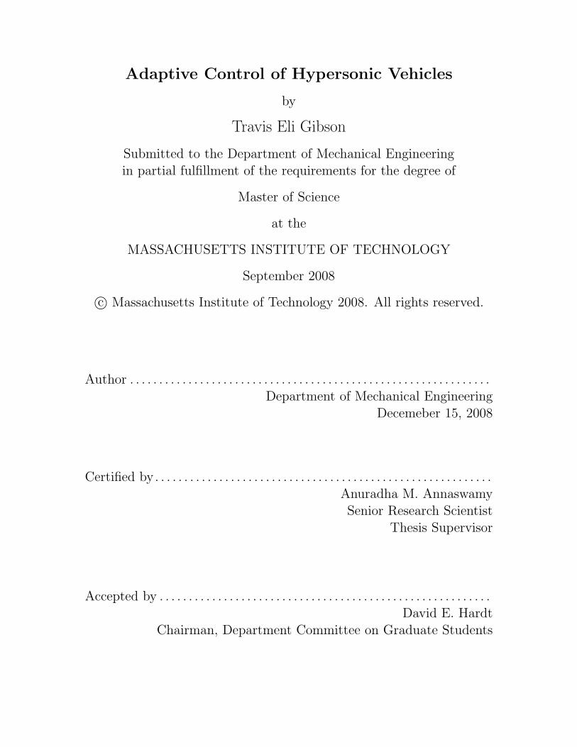
Adaptive Control of Hypersonic Vehicles
by
Travis Eli Gibson
Submitted to the Department of Mechanical Engineeringin partial fulfillment of the requirements for the degree of
Master of Science
at the
MASSACHUSETTS INSTITUTE OF TECHNOLOGY
September 2008
c© Massachusetts Institute of Technology 2008. All rights reserved.
Author . . . . . . . . . . . . . . . . . . . . . . . . . . . . . . . . . . . . . . . . . . . . . . . . . . . . . . . . . . . . . .Department of Mechanical Engineering
Decemeber 15, 2008
Certified by. . . . . . . . . . . . . . . . . . . . . . . . . . . . . . . . . . . . . . . . . . . . . . . . . . . . . . . . . .Anuradha M. AnnaswamySenior Research Scientist
Thesis Supervisor
Accepted by . . . . . . . . . . . . . . . . . . . . . . . . . . . . . . . . . . . . . . . . . . . . . . . . . . . . . . . . .David E. Hardt
Chairman, Department Committee on Graduate Students

2
Adaptive Control of Hypersonic Vehicles
by
Travis Eli Gibson
Submitted to the Department of Mechanical Engineeringon Decemeber 15, 2008, in partial fulfillment of the
requirements for the degree ofMaster of Science
Abstract
The Guidance, Navigation and Control of hypersonic vehicles are highly challeng-ing tasks due to the fact that the dynamics of the airframe, propulsion system andstructure are integrated and highly interactive. Such a coupling makes it difficult tomodel various components with a requisite degree of accuracy. This in turn makesvarious control tasks including altitude and velocity command tracking in the cruisephase of the flight extremely difficult. This work proposes an adaptive controller fora hypersonic cruise vehicle subject to: aerodynamic uncertainties, center-of-gravitymovements, actuator saturation, failures, and time-delays. The adaptive control ar-chitecture is based on a linearized model of the underlying rigid body dynamics andexplicitly accommodates for all uncertainties. Within the control structure is a base-line Proportional Integral Filter commonly used in optimal control designs. Thecontrol design is validated using a highfidelity HSV model that incorporates variouseffects including coupling between structural modes and aerodynamics, and thrustpitch coupling. Analysis of the Adaptive Robust Controller for Hypersonic Vehicles(ARCH) is carried out using a control verification methodology. This methodologyillustrates the resilience of the controller to the uncertainties mentioned above for aset of closed-loop requirements that prevent excessive structural loading, poor track-ing performance, and engine stalls. This analysis enables the quantification of theimprovements that result from using and adaptive controller for a typical maneuverin the V –h space under cruise conditions.
Thesis Supervisor: Anuradha M. AnnaswamyTitle: Senior Research Scientist
3

4

Acknowledgments
I would like to thank Dr. Anuradha Annaswamy for her continued support in my
research endeavors. I believe we will continue to generate great work together. Thank
you as well to Dr. Luis Crespo of the NIA for his research support. His work has
helped to illustrate the benefits of my research. I would also like to thank Dr. Sean
Kenny at NASA Langley for his direction during my summer work. I would like to
thank my lab mates: Yildiray Yildiz, Dr. Jinho Jang, Zac Dydek, Megumi Matsutani
and Manohar Srikanth. And of course my mom dad and brother for relaxing times
back in Florida. Finally I would like to thank God for helping me through my long
nights in lab, and these intense semesters at MIT.
5

6
Contents
1 Introduction 15
1.1 History of X–Planes . . . . . . . . . . . . . . . . . . . . . . . . . . . . 16
1.2 Modelling of Hypersonic Vehicles . . . . . . . . . . . . . . . . . . . . 18
1.3 Control Design . . . . . . . . . . . . . . . . . . . . . . . . . . . . . . 20
1.4 Overview . . . . . . . . . . . . . . . . . . . . . . . . . . . . . . . . . . 21
2 Vehicle Modelling 23
2.1 Oblique Shock and Expansion Wave Theory . . . . . . . . . . . . . . 24
2.2 Rigid Body Forces and Moments . . . . . . . . . . . . . . . . . . . . 26
2.3 Elastic Forces and Moments . . . . . . . . . . . . . . . . . . . . . . . 32
2.3.1 Natural Modes of Vibration for a Fixed–Free Beam . . . . . . 33
2.3.2 Forced Modal Response . . . . . . . . . . . . . . . . . . . . . 36
2.4 Equations of Motion . . . . . . . . . . . . . . . . . . . . . . . . . . . 37
2.4.1 Evaluation Model . . . . . . . . . . . . . . . . . . . . . . . . . 38
2.4.2 Design Model . . . . . . . . . . . . . . . . . . . . . . . . . . . 41
2.4.3 Actuator Dynamics . . . . . . . . . . . . . . . . . . . . . . . . 42
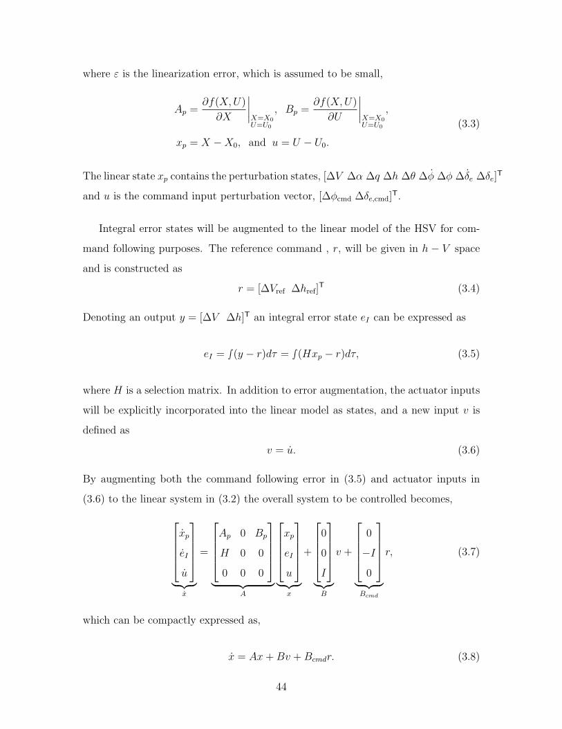
3 Controller Design 43
3.1 Linear Model . . . . . . . . . . . . . . . . . . . . . . . . . . . . . . . 43
3.2 Baseline Controller . . . . . . . . . . . . . . . . . . . . . . . . . . . . 45
3.3 Uncertainties and Actuator Saturation . . . . . . . . . . . . . . . . . 47
3.4 Adaptive Controller . . . . . . . . . . . . . . . . . . . . . . . . . . . . 49
7
4 Simulation Studies 53
5 Control Verification, A different Approach 63
5.1 Mathematical Framework . . . . . . . . . . . . . . . . . . . . . . . . 63
5.2 Hypersonic Vehicle Uncertainty . . . . . . . . . . . . . . . . . . . . . 65
5.3 Baseline Controller Analysis . . . . . . . . . . . . . . . . . . . . . . . 67
5.4 Adaptive Controller Analysis . . . . . . . . . . . . . . . . . . . . . . . 67
5.5 Comparative Analysis . . . . . . . . . . . . . . . . . . . . . . . . . . 68
6 Conclusions 71
A Tables 73
B Figures 77
C Control Design Parameters 103
8
List of Figures
1-1 Bell X–1 . . . . . . . . . . . . . . . . . . . . . . . . . . . . . . . . . . 16
1-2 X-15 . . . . . . . . . . . . . . . . . . . . . . . . . . . . . . . . . . . . 17
1-3 X–43 artistic rendering . . . . . . . . . . . . . . . . . . . . . . . . . . 18
1-4 X–43 on Pegasus under B–52B [6] . . . . . . . . . . . . . . . . . . . . 19
1-5 X–43 flight envelope [5] . . . . . . . . . . . . . . . . . . . . . . . . . . 20
2-1 HSV side view with control inputs[7] . . . . . . . . . . . . . . . . . . 23
2-2 HSV side view with dimenion labels[7] . . . . . . . . . . . . . . . . . 24
2-3 Visual aids for oblique shock and Prandtl–Meyer expansion.[2] . . . . 25
2-4 Mach Number Location Subscript Indexing . . . . . . . . . . . . . . . 27
2-5 Scramjet Model[7] . . . . . . . . . . . . . . . . . . . . . . . . . . . . . 29
2-6 Elastic HSV beam model with coordinates. . . . . . . . . . . . . . . . 32
2-7 Forward and aft mode shape. . . . . . . . . . . . . . . . . . . . . . . 36
2-8 Axes of the HSV . . . . . . . . . . . . . . . . . . . . . . . . . . . . . 39
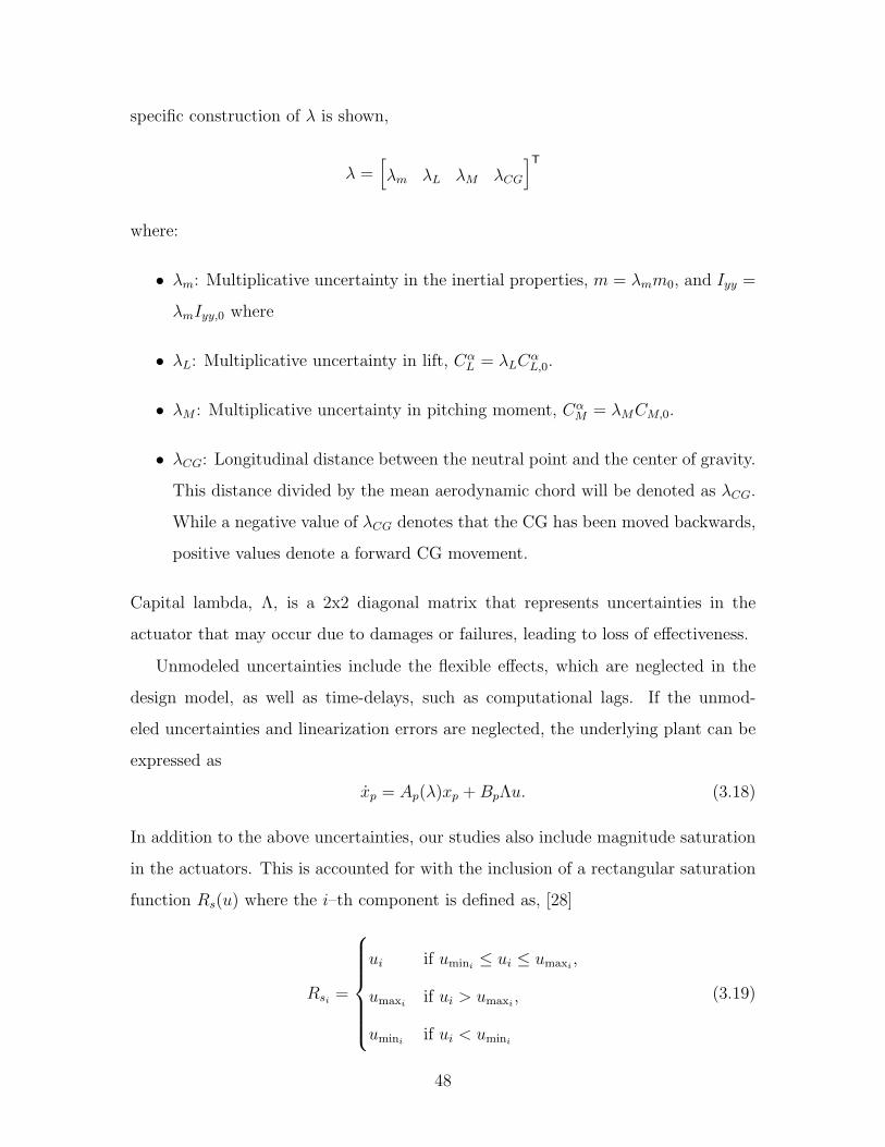
3-1 PIF control structure . . . . . . . . . . . . . . . . . . . . . . . . . . . 47
3-2 Nominal control structure . . . . . . . . . . . . . . . . . . . . . . . . 47
3-3 Uncertainty modelling . . . . . . . . . . . . . . . . . . . . . . . . . . 49
3-4 Nominal with adaptive augmentation and uncertainty . . . . . . . . . 50
3-5 Error Modelling . . . . . . . . . . . . . . . . . . . . . . . . . . . . . . 51
4-1 Pole Zero Map for φ δe to V γ. . . . . . . . . . . . . . . . . . . . . . . 54
4-2 Pole Zero Map zoom in at the origin. . . . . . . . . . . . . . . . . . . 55
4-3 Reference command in h–V space. . . . . . . . . . . . . . . . . . . . . 56
9
4-4 Command following errors for N1 and A1 simulation studies. . . . . . 57
4-5 Control input for N1 and A1 simulation studies. . . . . . . . . . . . . 57
4-6 Command following errors for N2 and A2 simulation studies. . . . . . 58
4-7 Control input for N2 and A2 simulation studies. . . . . . . . . . . . . 58
4-8 Command following errors for N3 and A3 simulation studies. . . . . . 59
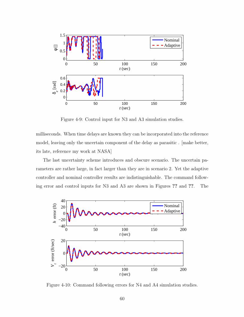
4-9 Control input for N3 and A3 simulation studies. . . . . . . . . . . . . 60
4-10 Command following errors for N4 and A4 simulation studies. . . . . . 60
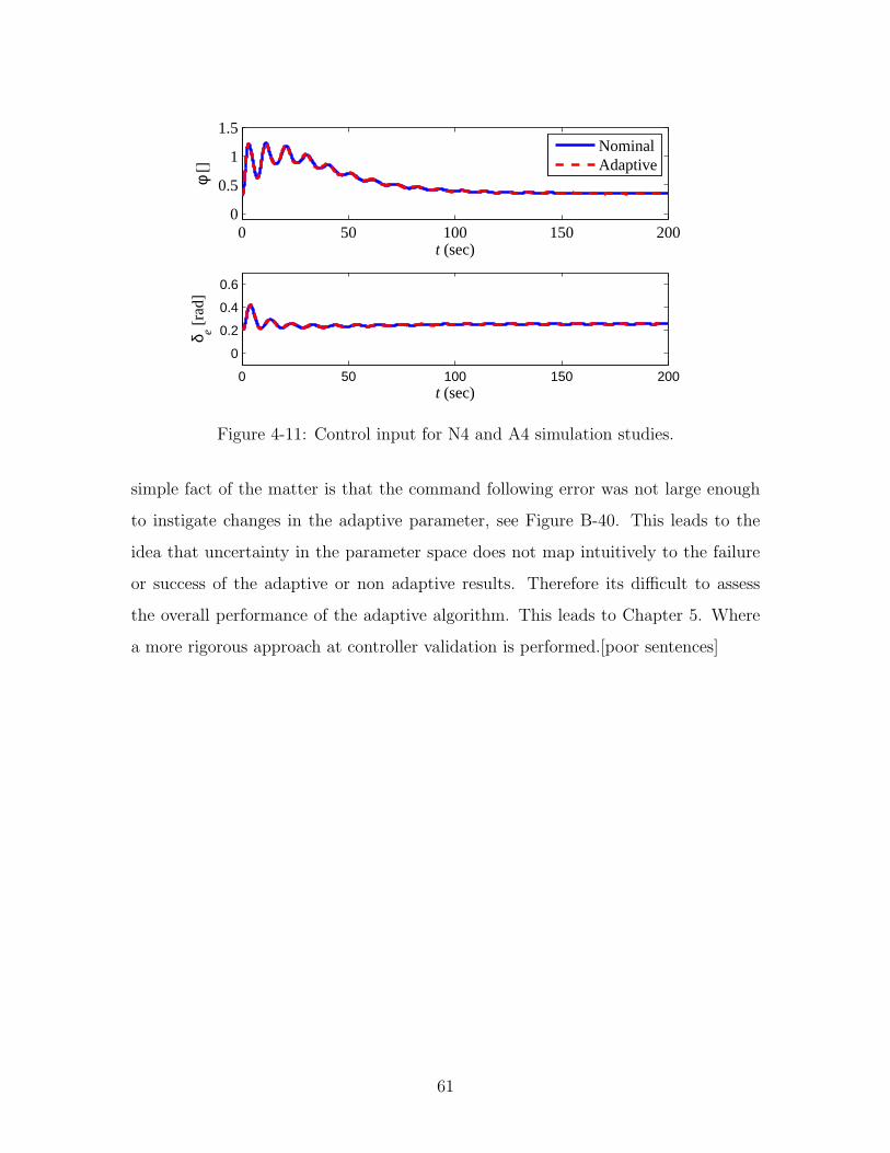
4-11 Control input for N4 and A4 simulation studies. . . . . . . . . . . . . 61
5-1 Failure and non-failure domains for the adaptive controller. . . . . . . 69
B-1 N1 Control inputs. . . . . . . . . . . . . . . . . . . . . . . . . . . . . 78
B-2 N1 Command following error. . . . . . . . . . . . . . . . . . . . . . . 78
B-3 N1 Rigid states. . . . . . . . . . . . . . . . . . . . . . . . . . . . . . . 79
B-4 N1 Loading Factor. . . . . . . . . . . . . . . . . . . . . . . . . . . . . 80
B-5 N1 Adaptive parameters. . . . . . . . . . . . . . . . . . . . . . . . . . 80
B-6 A1 Control inputs. . . . . . . . . . . . . . . . . . . . . . . . . . . . . 81
B-7 A1 Command following error. . . . . . . . . . . . . . . . . . . . . . . 81
B-8 A1 Rigid states. . . . . . . . . . . . . . . . . . . . . . . . . . . . . . . 82
B-9 A1 Loading Factor. . . . . . . . . . . . . . . . . . . . . . . . . . . . . 83
B-10 A1 Adaptive parameters. . . . . . . . . . . . . . . . . . . . . . . . . . 83
B-11 N2 Control inputs. . . . . . . . . . . . . . . . . . . . . . . . . . . . . 84
B-12 N2 Command following error. . . . . . . . . . . . . . . . . . . . . . . 84
B-13 N2 Rigid states. . . . . . . . . . . . . . . . . . . . . . . . . . . . . . . 85
B-14 N2 Loading Factor. . . . . . . . . . . . . . . . . . . . . . . . . . . . . 86
B-15 N2 Adaptive parameters. . . . . . . . . . . . . . . . . . . . . . . . . . 86
B-16 A2 Control inputs. . . . . . . . . . . . . . . . . . . . . . . . . . . . . 87
B-17 A2 Command following error. . . . . . . . . . . . . . . . . . . . . . . 87
B-18 A2 Rigid states. . . . . . . . . . . . . . . . . . . . . . . . . . . . . . . 88
B-19 A2 Loading Factor. . . . . . . . . . . . . . . . . . . . . . . . . . . . . 89
B-20 A2 Adaptive parameters. . . . . . . . . . . . . . . . . . . . . . . . . . 89
10
B-21 N3 Control inputs. . . . . . . . . . . . . . . . . . . . . . . . . . . . . 90
B-22 N3 Command following error. . . . . . . . . . . . . . . . . . . . . . . 90
B-23 N3 Rigid states. . . . . . . . . . . . . . . . . . . . . . . . . . . . . . . 91
B-24 N3 Loading Factor. . . . . . . . . . . . . . . . . . . . . . . . . . . . . 92
B-25 N3 Adaptive parameters. . . . . . . . . . . . . . . . . . . . . . . . . . 92
B-26 A3 Control inputs. . . . . . . . . . . . . . . . . . . . . . . . . . . . . 93
B-27 A3 Command following error. . . . . . . . . . . . . . . . . . . . . . . 93
B-28 A3 Rigid states. . . . . . . . . . . . . . . . . . . . . . . . . . . . . . . 94
B-29 A3 Loading Factor. . . . . . . . . . . . . . . . . . . . . . . . . . . . . 95
B-30 A3 Adaptive parameters. . . . . . . . . . . . . . . . . . . . . . . . . . 95
B-31 N4 Control inputs. . . . . . . . . . . . . . . . . . . . . . . . . . . . . 96
B-32 N4 Command following error. . . . . . . . . . . . . . . . . . . . . . . 96
B-33 N4 Rigid states. . . . . . . . . . . . . . . . . . . . . . . . . . . . . . . 97
B-34 N4 Loading Factor. . . . . . . . . . . . . . . . . . . . . . . . . . . . . 98
B-35 N4 Adaptive parameters. . . . . . . . . . . . . . . . . . . . . . . . . . 98
B-36 A4 Control inputs. . . . . . . . . . . . . . . . . . . . . . . . . . . . . 99
B-37 A4 Command following error. . . . . . . . . . . . . . . . . . . . . . . 99
B-38 A4 Rigid states. . . . . . . . . . . . . . . . . . . . . . . . . . . . . . . 100
B-39 A4 Loading Factor. . . . . . . . . . . . . . . . . . . . . . . . . . . . . 101
B-40 A4 Adaptive parameters. . . . . . . . . . . . . . . . . . . . . . . . . . 101
11

12
List of Tables
4.1 Trim values for two input HSV model. . . . . . . . . . . . . . . . . . 53
4.2 Simulation Study Uncertainty Selection. . . . . . . . . . . . . . . . . 56
5.1 1-dimensional CPVs for dbase. . . . . . . . . . . . . . . . . . . . . . . 67
5.2 1-dimensional CPVs for dadaptive. . . . . . . . . . . . . . . . . . . . . . 68
5.3 Relative PSM improvement. . . . . . . . . . . . . . . . . . . . . . . . 68
A.1 Geometry of Aircraft. . . . . . . . . . . . . . . . . . . . . . . . . . . . 73
A.2 Physical Constants and Aerodynamic Coefficients. [39, 20] . . . . . . 74
A.3 Trim values for two input HSV model. . . . . . . . . . . . . . . . . . 75
A.4 Eigenvalues and Modes of HSV. . . . . . . . . . . . . . . . . . . . . . 75
13

14
Chapter 1
Introduction
“Not since the Right Brothers solved the basic problems of sustained,
controlled flight has there been such an assault upon our atmosphere as
during the first years of the space age. Man extended and speeded up
his travels within the vast ocean of air surrounding the Earth until he
achieved flight outside its confines. This remarkable accomplishment was
the culmination of a long history of effort to harness the force of that
air so that he could explore the three-dimensional ocean of atmosphere
in which he lives. That history had shown him that before he could ex-
plore his ethereal ocean, he must first explore the more restrictive world
of aerodynamic forces.”[45]
Wendell H. Stillwell
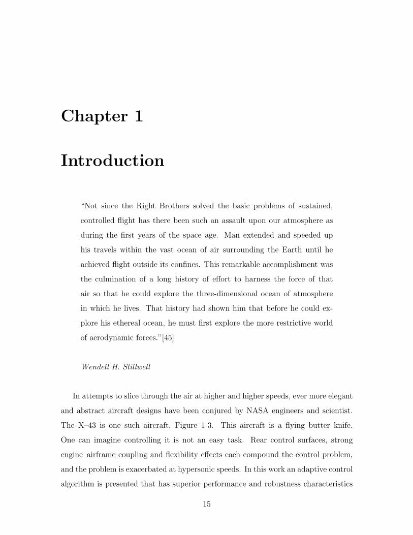
In attempts to slice through the air at higher and higher speeds, ever more elegant
and abstract aircraft designs have been conjured by NASA engineers and scientist.
The X–43 is one such aircraft, Figure 1-3. This aircraft is a flying butter knife.
One can imagine controlling it is not an easy task. Rear control surfaces, strong
engine–airframe coupling and flexibility effects each compound the control problem,
and the problem is exacerbated at hypersonic speeds. In this work an adaptive control
algorithm is presented that has superior performance and robustness characteristics
15
when compared to a nominal classic controller.
1.1 History of X–Planes
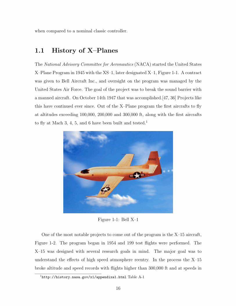
The National Advisory Committee for Aeronautics (NACA) started the United States
X–Plane Program in 1945 with the XS–1, later designated X–1, Figure 1-1. A contract
was given to Bell Aircraft Inc., and oversight on the program was managed by the
United States Air Force. The goal of the project was to break the sound barrier with
a manned aircraft. On October 14th 1947 that was accomplished.[47, 36] Projects like
this have continued ever since. Out of the X–Plane program the first aircrafts to fly
at altitudes exceeding 100,000, 200,000 and 300,000 ft, along with the first aircrafts
to fly at Mach 3, 4, 5, and 6 have been built and tested.1
Figure 1-1: Bell X–1
One of the most notable projects to come out of the program is the X–15 aircraft,
Figure 1-2. The program began in 1954 and 199 test flights were performed. The
X–15 was designed with several research goals in mind. The major goal was to
understand the effects of high speed atmosphere reentry. In the process the X–15
broke altitude and speed records with flights higher than 300,000 ft and at speeds in
1http://history.nasa.gov/x1/appendixa1.html Table A-1
16
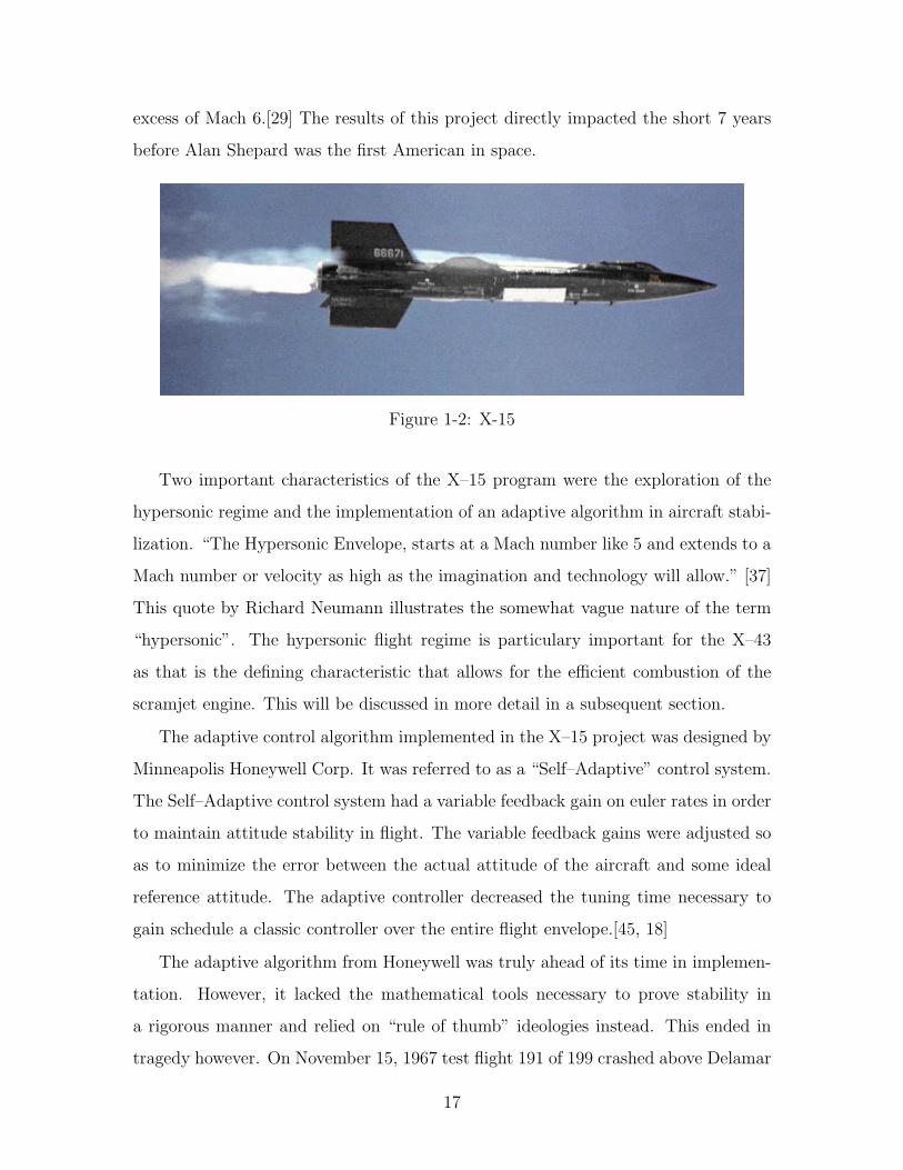
excess of Mach 6.[29] The results of this project directly impacted the short 7 years
before Alan Shepard was the first American in space.
Figure 1-2: X-15
Two important characteristics of the X–15 program were the exploration of the
hypersonic regime and the implementation of an adaptive algorithm in aircraft stabi-
lization. “The Hypersonic Envelope, starts at a Mach number like 5 and extends to a
Mach number or velocity as high as the imagination and technology will allow.” [37]
This quote by Richard Neumann illustrates the somewhat vague nature of the term
“hypersonic”. The hypersonic flight regime is particulary important for the X–43
as that is the defining characteristic that allows for the efficient combustion of the
scramjet engine. This will be discussed in more detail in a subsequent section.
The adaptive control algorithm implemented in the X–15 project was designed by
Minneapolis Honeywell Corp. It was referred to as a “Self–Adaptive” control system.
The Self–Adaptive control system had a variable feedback gain on euler rates in order
to maintain attitude stability in flight. The variable feedback gains were adjusted so
as to minimize the error between the actual attitude of the aircraft and some ideal
reference attitude. The adaptive controller decreased the tuning time necessary to
gain schedule a classic controller over the entire flight envelope.[45, 18]
The adaptive algorithm from Honeywell was truly ahead of its time in implemen-
tation. However, it lacked the mathematical tools necessary to prove stability in
a rigorous manner and relied on “rule of thumb” ideologies instead. This ended in
tragedy however. On November 15, 1967 test flight 191 of 199 crashed above Delamar
17
Dry Lake.[29] Unbeknownst to the pilot there was an electrical malfunction and the
aircraft began to deviate from the desired trajectory and a gross side–slip angle was
building. Once off by 15 the pilot corrected for the mistake, then the aircraft drifted
again, after several seconds of pilot corrections the aircraft interred a Mach 5 spin
at an altitude of 230,000 ft.[29, 46] As the aircraft fell into more dense air it broke
apart killing the pilot, Mike Adams. This crash put a holt on all adaptive control
implementation for several decades, and not until recently has the idea been revisited.
Now with more rigorous stability proofs.
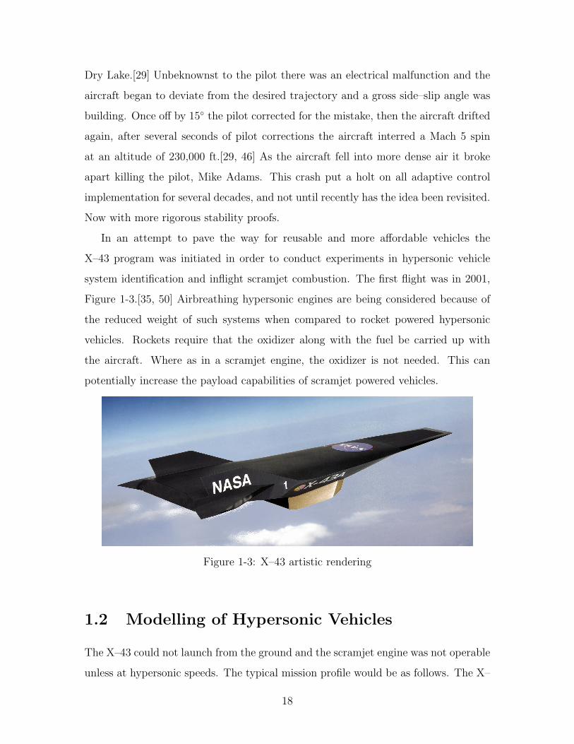
In an attempt to pave the way for reusable and more affordable vehicles the
X–43 program was initiated in order to conduct experiments in hypersonic vehicle
system identification and inflight scramjet combustion. The first flight was in 2001,
Figure 1-3.[35, 50] Airbreathing hypersonic engines are being considered because of
the reduced weight of such systems when compared to rocket powered hypersonic
vehicles. Rockets require that the oxidizer along with the fuel be carried up with
the aircraft. Where as in a scramjet engine, the oxidizer is not needed. This can
potentially increase the payload capabilities of scramjet powered vehicles.
Figure 1-3: X–43 artistic rendering
1.2 Modelling of Hypersonic Vehicles
The X–43 could not launch from the ground and the scramjet engine was not operable
unless at hypersonic speeds. The typical mission profile would be as follows. The X–
18
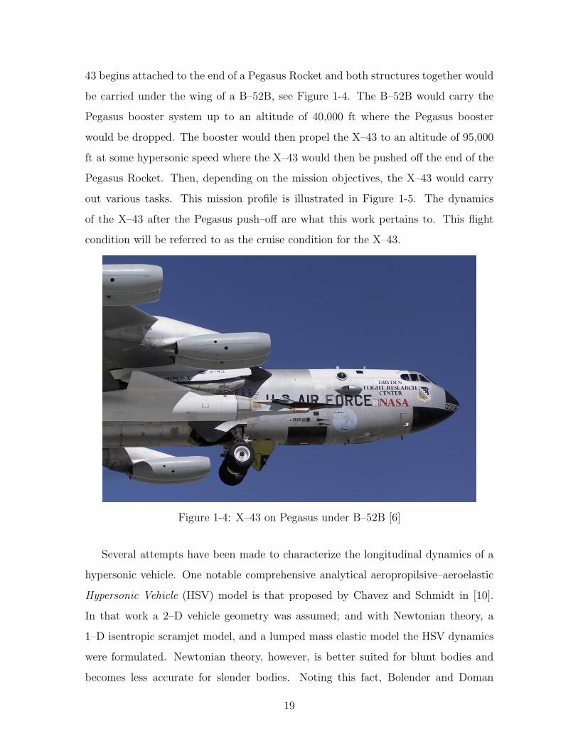
43 begins attached to the end of a Pegasus Rocket and both structures together would
be carried under the wing of a B–52B, see Figure 1-4. The B–52B would carry the
Pegasus booster system up to an altitude of 40,000 ft where the Pegasus booster
would be dropped. The booster would then propel the X–43 to an altitude of 95,000
ft at some hypersonic speed where the X–43 would then be pushed off the end of the
Pegasus Rocket. Then, depending on the mission objectives, the X–43 would carry
out various tasks. This mission profile is illustrated in Figure 1-5. The dynamics
of the X–43 after the Pegasus push–off are what this work pertains to. This flight
condition will be referred to as the cruise condition for the X–43.
Figure 1-4: X–43 on Pegasus under B–52B [6]
Several attempts have been made to characterize the longitudinal dynamics of a
hypersonic vehicle. One notable comprehensive analytical aeropropilsive–aeroelastic
Hypersonic Vehicle (HSV) model is that proposed by Chavez and Schmidt in [10].
In that work a 2–D vehicle geometry was assumed; and with Newtonian theory, a
1–D isentropic scramjet model, and a lumped mass elastic model the HSV dynamics
were formulated. Newtonian theory, however, is better suited for blunt bodies and
becomes less accurate for slender bodies. Noting this fact, Bolender and Doman
19
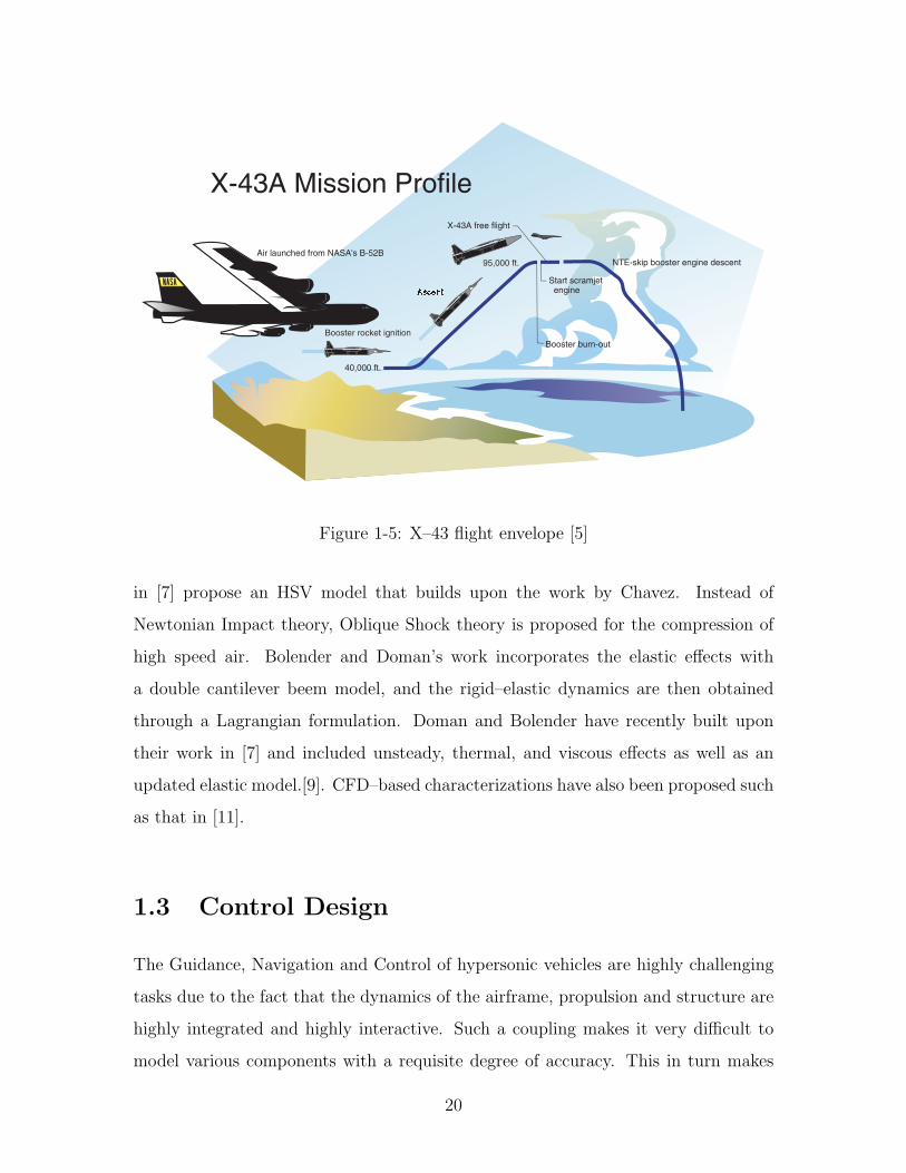
Figure 1-5: X–43 flight envelope [5]
in [7] propose an HSV model that builds upon the work by Chavez. Instead of
Newtonian Impact theory, Oblique Shock theory is proposed for the compression of
high speed air. Bolender and Doman’s work incorporates the elastic effects with
a double cantilever beem model, and the rigid–elastic dynamics are then obtained
through a Lagrangian formulation. Doman and Bolender have recently built upon
their work in [7] and included unsteady, thermal, and viscous effects as well as an
updated elastic model.[9]. CFD–based characterizations have also been proposed such
as that in [11].
1.3 Control Design
The Guidance, Navigation and Control of hypersonic vehicles are highly challenging
tasks due to the fact that the dynamics of the airframe, propulsion and structure are
highly integrated and highly interactive. Such a coupling makes it very difficult to
model various components with a requisite degree of accuracy. This in turn makes
20
various control tasks including altitude and velocity command tracking in the cruise
phase of the flight extremely difficult.
Notable works in the area of HSV control design are discussed here in. In [32], an
adaptive linear-quadratic controller is deployed in the presence of structural modes
and actuator dynamics, and is shown to track altitude and velocity commands in
the presence of aerodynamic changes and actuator changes. The authors of [51]
designed an adaptive sliding mode controller that tracks step commands in height
and velocity while requiring limited state information. In [19] the authors employed
both robust and adaptive techniques on a sequential loop closing methodology. The
work in [30] focuses on elastic mode suppression through an adaptive notch filter
technique. References [34], [48] and [49] not only focus on control design but also
on robustness characteristics of the controller. Similar studies are carried out in this
thesis in Chapter 5. Other notable works in TeX area of control of Hypersonic vehicles
are References [33, 1, 25, 13, 12, 23, 40, 38, 22, 39, 41] and [31].
Uncertainty characterization is also important when determining the relative ro-
bustness characteristics of any given controller. Aircraft geometry and mass property
uncertainties have been studied in [38]. Aerodynamics coefficient uncertainties were
used in [39] and [32] to test the control algorithm; and inertial–elastic uncertainties
were studied in [41] and [27].
1.4 Overview
In this work, a baseline controller is first developed that has Proportional, Integral
and Filter components, commonly called a PIF controller.[43] An adaptive controller
then augments to the baseline controller. It accommodates for aerodynamic uncer-
tainties, center-of-gravity movements, actuator saturation and failures and is robust
with respect to time–delays and elastic effects. The nonlinear rigid HSV model in
[39] is used for control design and the nonlinear aeroelastic HSV model in [7] is used
for controller evaluation. Time simulations are presented to illustrate the benefits of
the adaptive algorithm. Analysis is also performed in order to study the resilience
21

of the controller to the uncertainties mentioned above for a set of closed-loop re-
quirements that prevent excessive structural loading, poor tracking performance and
engine stalls.[21, ?]
22
Chapter 2
Vehicle Modelling
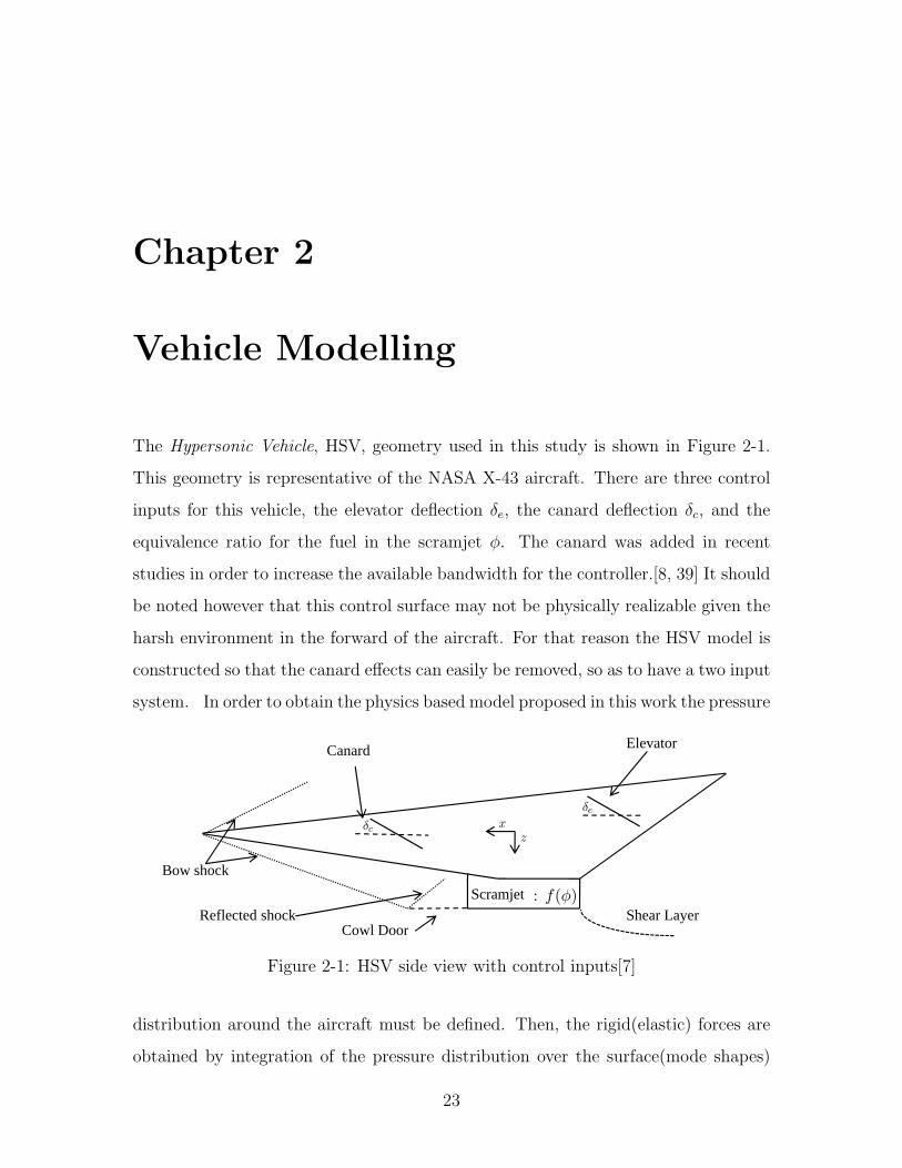
The Hypersonic Vehicle, HSV, geometry used in this study is shown in Figure 2-1.
This geometry is representative of the NASA X-43 aircraft. There are three control
inputs for this vehicle, the elevator deflection δe, the canard deflection δc, and the
equivalence ratio for the fuel in the scramjet φ. The canard was added in recent
studies in order to increase the available bandwidth for the controller.[8, 39] It should
be noted however that this control surface may not be physically realizable given the
harsh environment in the forward of the aircraft. For that reason the HSV model is
constructed so that the canard effects can easily be removed, so as to have a two input
system. In order to obtain the physics based model proposed in this work the pressure
Lx; U
V
θ γ
L; U
Fx; T
DFz
z,W
ElevatorCanard
±e
xz
±c
ScramjetShear Layer
Bow shock
: f(Á)
Cowl Door Reflected shock
1
Figure 2-1: HSV side view with control inputs[7]
distribution around the aircraft must be defined. Then, the rigid(elastic) forces are
obtained by integration of the pressure distribution over the surface(mode shapes)
23
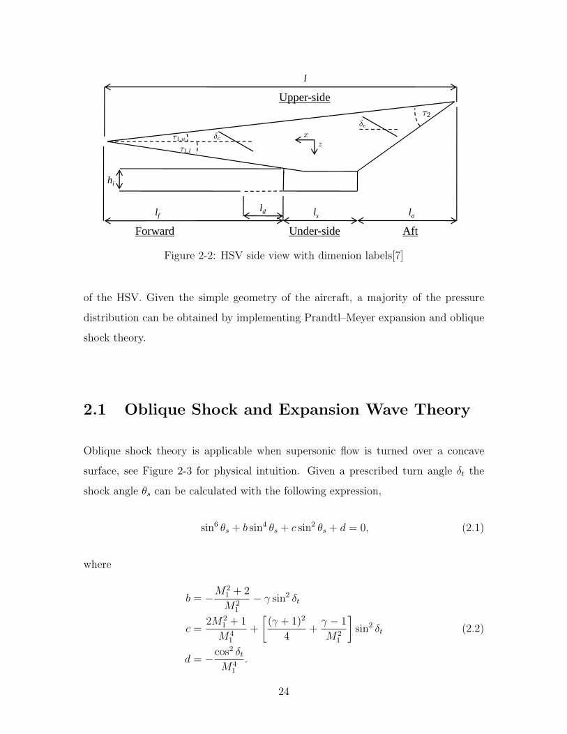
¿2
Upper-side
±e
x±
l
¿1;ux
z±c
¿1;l
hi
Forward Under-side Aft
lf ls lald
Figure 2-2: HSV side view with dimenion labels[7]
of the HSV. Given the simple geometry of the aircraft, a majority of the pressure
distribution can be obtained by implementing Prandtl–Meyer expansion and oblique
shock theory.
2.1 Oblique Shock and Expansion Wave Theory
Oblique shock theory is applicable when supersonic flow is turned over a concave
surface, see Figure 2-3 for physical intuition. Given a prescribed turn angle δt the
shock angle θs can be calculated with the following expression,
sin6 θs + b sin4 θs + c sin2 θs + d = 0, (2.1)
where
b = −M21 + 2
M21
− γ sin2 δt
c =2M2
1 + 1
M41
+
[(γ + 1)2
4+γ − 1
M21
]sin2 δt
d = −cos2 δtM4
1
.
(2.2)
24

In the previous expression M1 denotes the mach number of the fluid before reaching
the shock wave and γ represents the ratio of specific heats (γ = Cp/Cv). The shock
angle is then determined by solving for the second root of Equation (2.1) with respect
to sin2 θs. The pressure p, temperature T , and Mach number M , can then be obtained
using the relations,
p2
p1
=7M2
1 sin2 θs − 1
6(2.3)
T2
T1
=
(7M2
1 sin2 θs − 1)(M2
1 sin2 θs + 5)
36M21 sin θs
(2.4)
M22 sin2(θs − δt) =
M21 sin2 θs + 5
7M21 sin2 θs − 1
. (2.5)
where subscripts 1 and 2 denote pre and post shock values.[3]
Oblique Shock Theory
Shock Line
M1 > M2
p1 < p2
T1 < T2
Constant Entropy Expansion Fan
Prandtl-Meyer Expansion
M1 < M2p1 > p2
T1 > T2
12 1
2
Figure 2-3: Visual aids for oblique shock and Prandtl–Meyer expansion.[2]
When the opposite scenario occurs and flow is turned over a convex corner, the
flow expands. The properties of the gas are then characterized by Prandtl–Meyer
expansion,
δt = ν(M2)− ν(M1) (2.6)
where
ν(M) =
√γ + 1
γ − 1arctan
√γ + 1
γ − 1
(M2 − 1
)arctan
√M2 − 1. (2.7)
With the post expansion Mach number obtained, the remaining air properties can be
25
calculated as,[3]
p2
p1
=
[1 + [(γ − 1)/2]M2
1
1 + [(γ − 1)/2]M22
]γ/(γ−1)
(2.8)
T2
T1
=1 + [(γ − 1)/2]M2
1
1 + [(γ − 1)/2]M22
. (2.9)
These theories can then be applied across the front, top and bottom of the aircraft
in order to obtain the pressure distribution for the upper-surface, forward, underside,
and inlet to the scramjet as well as the air properties around the canard and elevator.
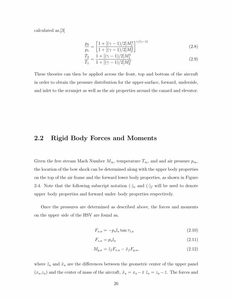
2.2 Rigid Body Forces and Moments
Given the free stream Mach Number M∞, temperature T∞, and and air pressure p∞,
the location of the bow shock can be determined along with the upper body properties
on the top of the air frame and the forward lower body properties, as shown in Figure
2-4. Note that the following subscript notation (·)u and (·)f will be used to denote
upper–body properties and forward under–body properties respectively.
Once the pressures are determined as described above, the forces and moments
on the upper–side of the HSV are found as,
Fx,u = −pulu tan τ1,u (2.10)
Fz,u = pulu (2.11)
My,u = zfFx,u − xfFy,u, (2.12)
where zu and xu are the differences between the geometric center of the upper panel
(xu,zu) and the center of mass of the aircraft, xu = xu− x zu = zu− z. The forces and
26
moments on the forward under–side are then found using the following expressions,
Fx,f = −pf ll tan τ1,l (2.13)
Fz,f = −pf ll (2.14)
My,f = zfFx,f − xfFy,f , (2.15)
with zf and xf having the same interpretation as above. The pressure is constant on
the surface of the HSV behind the bow shock and it is for that reason that the forces
are simply calculated using a single value for the pressure across the entire surface.
Lx; U
V
θ γ
L; U
Fx; T
DFz
z,W
xz
M
Ma
Mu
Mc;u
Mc;l
Me;l
Me;u
M1
Mf
Mi
Mn
®
±d
1
Figure 2-4: Mach Number Location Subscript Indexing
The air after passing through the bow shock on the under–side of the HSV will
impinge on the cowl door, which protrudes in front of the scramjet engine. The cowl
door is assumed to be adjustable and in this work it is assumed that the cowl door
can be adjusted perfectly so as to maintain an on lip condition with the bow shock
wave. Given this scenario, there will be a force exerted on the aircraft as the post
bow shock air is turned parallel to the entrance of the scramjet,
Fx,inlet = γM2f pf (1− cos(τ1,l + α))hi (2.16)
Fz,inlet = γM2f pf sin(τ1,l + α)hi (2.17)
My,inlet = zinletFx,inlet − xinletFz,inlet. (2.18)
Using geometry, one would find that the cowl door is adjusted using the following
27
expression,
ld = lf − (lf tan τ1,l + hi) cot(δd − α), (2.19)
where δd is the relative angle between the bow shock and the cowl door, and α is the
angle of attack of the aircraft.
The nacelle is the cowl door and the underside of the scramjet together, and
properties of the aircraft under the nacelle are denoted as (·)n. The nacelle length is
given as,
ln = ls + ld.
The total force and moment imparted on the nacelle of the aircraft is determined by
the following relations,
Fz,n = −pnln (2.20)
My,n = −Fz,nxn, (2.21)
where xn is distance between the center of the nacelle and the center of gravity of the
aircraft, and pn is calculated using either oblique shock theory or expansion theory
depending on the angle of attack. Note that given the shock on lip condition, the
properties for the nacelle are simply determined from the free stream air. If the shock
on lip condition is not satisfied, the above relations do not hold.
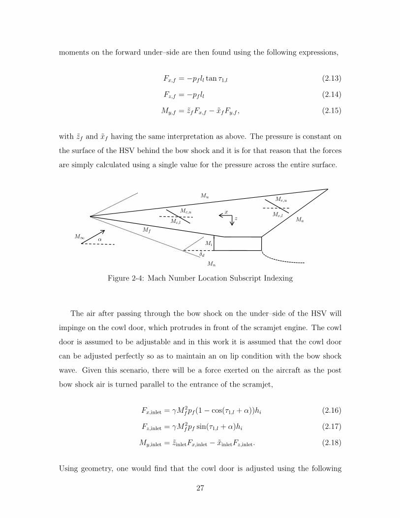
Continuing to follow the path of the air. After it passing through the bow shock
and then the second shock from the reflection on the cowl door, the air will enter the
scramjet engine. The scramjet is modelled as 1-D, and isentropic flow is assumed. The
expressions necessary to incorporate the propulsion system were first introduced by
Chavez and Schmidt.[10] The model for the scramjet is shown in Figure 2-5. After the
free stream air impinges on the front of the HSV, it is turned under and is parallel to
the forebody of the aircraft. Oblique Shock theory can be used in order to determine
the Mach Number at the Inlet from the Mach Number under the fore-body of the
HSV.
The change in Mach number as the flow is compressed in the diffuser is calculated
28
Reflecting Shock Wave
Combustor NozzleDiffuserhi hci hce heMf Mi
Ad = hci=hi An = he=hce
ci ei ceCowl Door
Figure 2-5: Scramjet Model[7]
as,
[1 + [(γ − 1)/2]M2
ci
](γ+1)/(γ−1)
M2ci
= A2d
[1 + [(γ − 1)/2]M2
i
](γ+1)/(γ−1)
M2i
(2.22)
where (·)i denotes the inlet to the scramjet, (·)ci denotes the combustor inlet, and Ad
is the diffuser area ratio as shown in Figure 2-5. The air properties at the combustor
inlet are calculated using Equations (2.8) and (2.9).
The combustor is modelled as a constant area duct with heat addition. This leads
to the expression,
M2ce
[1 + [(γ − 1)/2]M2
ce
](γM2
ce + 1)2=M2
ci
[1 + [(γ − 1)/2]M2
ci
](γM2
ci + 1)2+
M2ci
(γM2ci + 1)2
∆TtcTci
(2.23)
where the Mach number at the combustor exit Mce is a function of the total tem-
perature change across the combustor∆Ttc . The temperature and pressure at the
combustor exit are then defined as
pce = pci1 + γM2
ci
1 + γM2ce
(2.24)
Tce = Tci
[(1 + γM2
ce
1 + γM2ci
)Mci
Mi
]2
(2.25)
An analytical expression relating the total temperature change across the com-
29
bustor to the equivalence ratio φ follows,
Ttce
Ttci
=1 +Hfηcfstφ/(cpTtci
)
1 + fsTφ(2.26)
∆Ttc = Ttce − Ttci(2.27)
where ηc is the efficiency of the scramjet (0.9), fst is the stoichiometric air-fuel ratio
(0.0291), Hc is the heat of combustion for the fuel (LH2 at 51,500 BTU/lbm) and cp
is the specific heat of the fuel at constant pressure (0.24 BTU/(lbmR).[24, 26, 4, 7]
It is important to note that temperatures with subscript t are the total temperatures
and all other temperatures referred to in this work are the static temperatures. The
ratio of total temperature to static temperature can be obtained using the following,
TtT
= 1 +γ − 1
2M2. (2.28)
The procedure for obtaining the Mach number for the air at the exit of the scramjet
is similar to that of Equation (2.22),
[1 + [(γ − 1)/2]M2
e
](γ+1)/(γ−1)
M2e
= A2n
[1 + [(γ − 1)/2]M2
ce
](γ+1)/(γ−1)
M2ce
. (2.29)
Using a control volume around the scramjet and applying the law of conservation of
momentum, the total thrust from the scramjet can be obtained
T = ma(Ve − V∞) + (pe − p∞)he − (pi − p∞)hi. (2.30)
The air upon leaving the scramjet will then expand along the aft of the aircraft
and interact with the free stream air coming from the underside of the HSV. An
analytical expression for the pressure on the aft of the scramjet as a function of the
free stream air pressure was found by Chavez and Schmidt and is displayed below,
pa =pe
1 + sa/la(pe/p∞ − 1)(2.31)
30
where la is the length of the aft of the aircraft in the x–body direction and sa is the
length coordinate in the x–body direction. Integration of the aft body pressure along
the back side of the aircraft results into the following expressions for the aft-body
forces and moments,
Fx,a = p∞lapep∞
log(pe/p∞)
(pe/p∞)− 1tan(τ2 + τ1,u (2.32)
Fz,a = −p∞lapep∞
log(pe/p∞)
(pe/p∞)− 1(2.33)
My,a = zaFx,a − xaFz,a (2.34)
where the pitching moment is calculated from the point of average pressure on the aft
body panel. The point of average pressure can be calculated as pa = ∫ la0 pa(sa)dsa/la.
The center of pressure coordinates are then found by solving for xa in the following
expression pa(xa) = pa. Then the relative position of the center of pressure to the
center of gravity of the HSV is trivial.
Two components of the total force acting on the HSV that have not been ad-
dressed yet are the forces from the canard and elevator. Depending on the angle of
attack of the HSV and the relative positions of the canard and elevator the pressure
surrounding the control surfaces can be determined from oblique shock or Prandtl–
Meyer expansion. Once the pressures surrounding the canard are determined, the
forces acting upon it are calculated as follows,
Fx,c =− (pc,l − pc,u) sin δcSc (2.35)
Fz,c =− (pc,l − pc,u) cos δcSc (2.36)
My,c =zcFx,c − xcFz,c. (2.37)
The forces acting on the elevator have an identical set of equations and are shown
31
below for completeness,
Fx,e =− (pe,l − pe,u) sin δeSe (2.38)
Fz,e =− (pe,l − pe,u) cos δeSe (2.39)
My,e =zeFx,e − xeFz,e. (2.40)
For the coordinates of the canard and elevator refer to Appendix A.1.
Thus far all of the forces and moments acting on the hypersonic vehicle that
control the rigid–body dynamics have been expressed and therefore the total x–body
force, z–body force and y–body moment are calculated as follows,
Fx = Fx,u + Fx,f + Fx,inlet + Fx,a + Fx,e + Fx,c (2.41)
Fz = Fz,u + Fz,f + Fz,inlet + Fz,n + Fz,a + Fz,e + Fz,c (2.42)
My = My,u +My,f +My,inlet +My,n +My,a +My,e +My,c + zT T . (2.43)
As previously mentioned, this work also includes the elastic effects an the HSV dy-
namics. These effects are outlined in the following section.
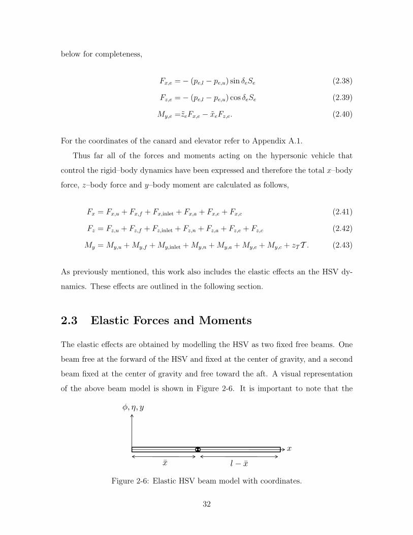
2.3 Elastic Forces and Moments
The elastic effects are obtained by modelling the HSV as two fixed free beams. One
beam free at the forward of the HSV and fixed at the center of gravity, and a second
beam fixed at the center of gravity and free toward the aft. A visual representation
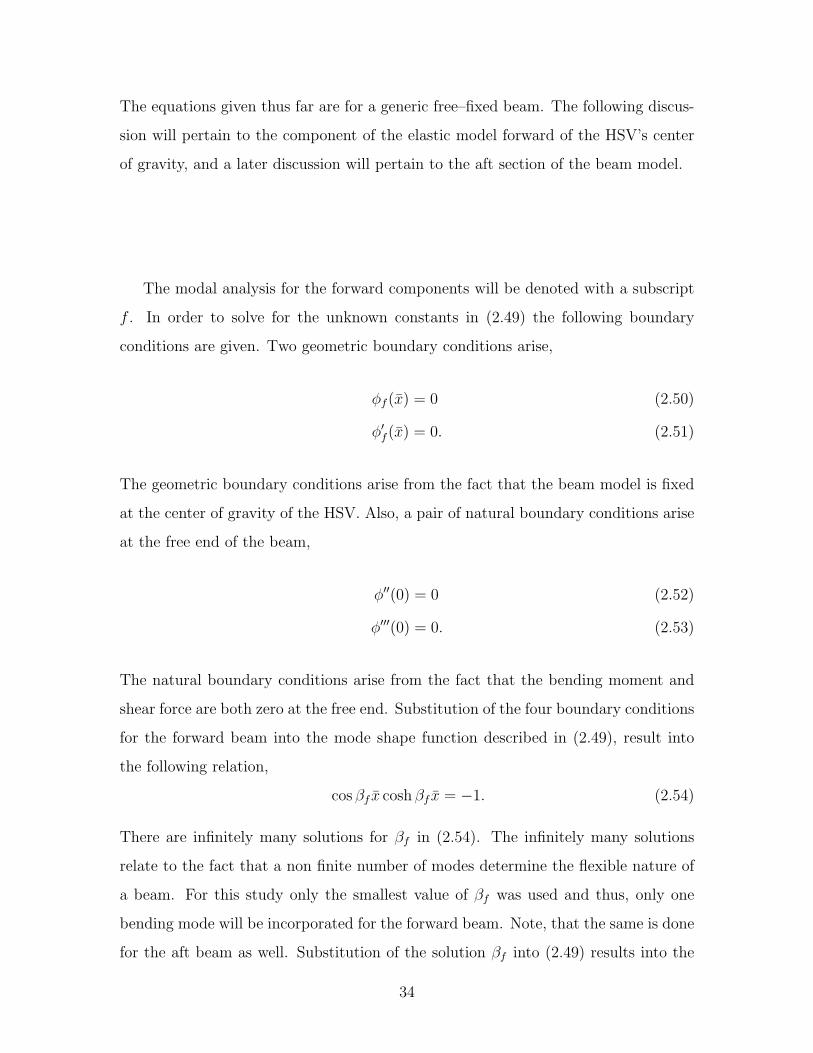
of the above beam model is shown in Figure 2-6. It is important to note that the
Á; ´; y
x
l¡ ¹x¹x
Figure 2-6: Elastic HSV beam model with coordinates.
32
coordinate system for the elastic model has up as positive, where in the rigid–body
model down is positive.
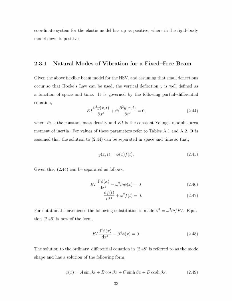
2.3.1 Natural Modes of Vibration for a Fixed–Free Beam
Given the above flexible beam model for the HSV, and assuming that small deflections
occur so that Hooke’s Law can be used, the vertical deflection y is well defined as
a function of space and time. It is governed by the following partial–differential
equation,
EI∂4y(x, t)
∂x4+ m
∂2y(x, t)
∂t2= 0, (2.44)
where m is the constant mass density and EI is the constant Young’s modulus area
moment of inertia. For values of these parameters refer to Tables A.1 and A.2. It is
assumed that the solution to (2.44) can be separated in space and time so that,
y(x, t) = φ(x)f(t). (2.45)
Given this, (2.44) can be separated as follows,
EId4φ(x)
dx4− ω2mφ(x) = 0 (2.46)
df(t)
dt4+ ω2f(t) = 0. (2.47)
For notational convenience the following substitution is made β4 = ω2m/EI. Equa-
tion (2.46) is now of the form,
EId4φ(x)
dx4− β4φ(x) = 0. (2.48)
The solution to the ordinary–differential equation in (2.48) is referred to as the mode
shape and has a solution of the following form,
φ(x) = A sin βx+B cos βx+ C sinh βx+D cosh βx. (2.49)
33
The equations given thus far are for a generic free–fixed beam. The following discus-
sion will pertain to the component of the elastic model forward of the HSV’s center
of gravity, and a later discussion will pertain to the aft section of the beam model.
The modal analysis for the forward components will be denoted with a subscript
f . In order to solve for the unknown constants in (2.49) the following boundary
conditions are given. Two geometric boundary conditions arise,
φf (x) = 0 (2.50)
φ′f (x) = 0. (2.51)
The geometric boundary conditions arise from the fact that the beam model is fixed
at the center of gravity of the HSV. Also, a pair of natural boundary conditions arise
at the free end of the beam,
φ′′(0) = 0 (2.52)
φ′′′(0) = 0. (2.53)
The natural boundary conditions arise from the fact that the bending moment and
shear force are both zero at the free end. Substitution of the four boundary conditions
for the forward beam into the mode shape function described in (2.49), result into
the following relation,
cos βf x cosh βf x = −1. (2.54)
There are infinitely many solutions for βf in (2.54). The infinitely many solutions
relate to the fact that a non finite number of modes determine the flexible nature of
a beam. For this study only the smallest value of βf was used and thus, only one
bending mode will be incorporated for the forward beam. Note, that the same is done
for the aft beam as well. Substitution of the solution βf into (2.49) results into the
34
following expression for the forward beam mode shape,
φf =Af [(sin βf x− sinh βf x)(sin βfx+ sinh βfx)
+ (cos βf x+ cosh βf x)(cos βfx+ cosh βfx)],(2.55)
where Af is a scaling factor that is chosen so as to mass normalize the mode shape
and is determined by the following orthogonal solution,
∫ x
0
mfφf (x)φf (x)dx = 1. (2.56)
A similar approach was taken for the aft cantilever beam. With its unique set of
four boundary conditions, the following relation results
cos(βa(l − x)) cosh(βa(l − x)) = −1, (2.57)
so that the aft beam has a mode shape of the following form,
φa =Aa[(sin βa(l − x)− sinh βa(l − x))(sin βa(x− x)− sinh βa(x− x))
+ (cos βa(l − x) + cosh βa(l − x))(cos βa(x− x)− cosh βa(x− x))].(2.58)
The aft beam is also mass normalized, and Aa is solved for in the following,
∫ l
x
maφa(x)φa(x)dx = 1. (2.59)
Using the above approach, the following values were obtained for the forward and
aft beams,
Af = 0.0283 ft
Aa = −0.0256 ft
βf = 0.0341 ft−1
βa = 0.0417 ft−1.
35
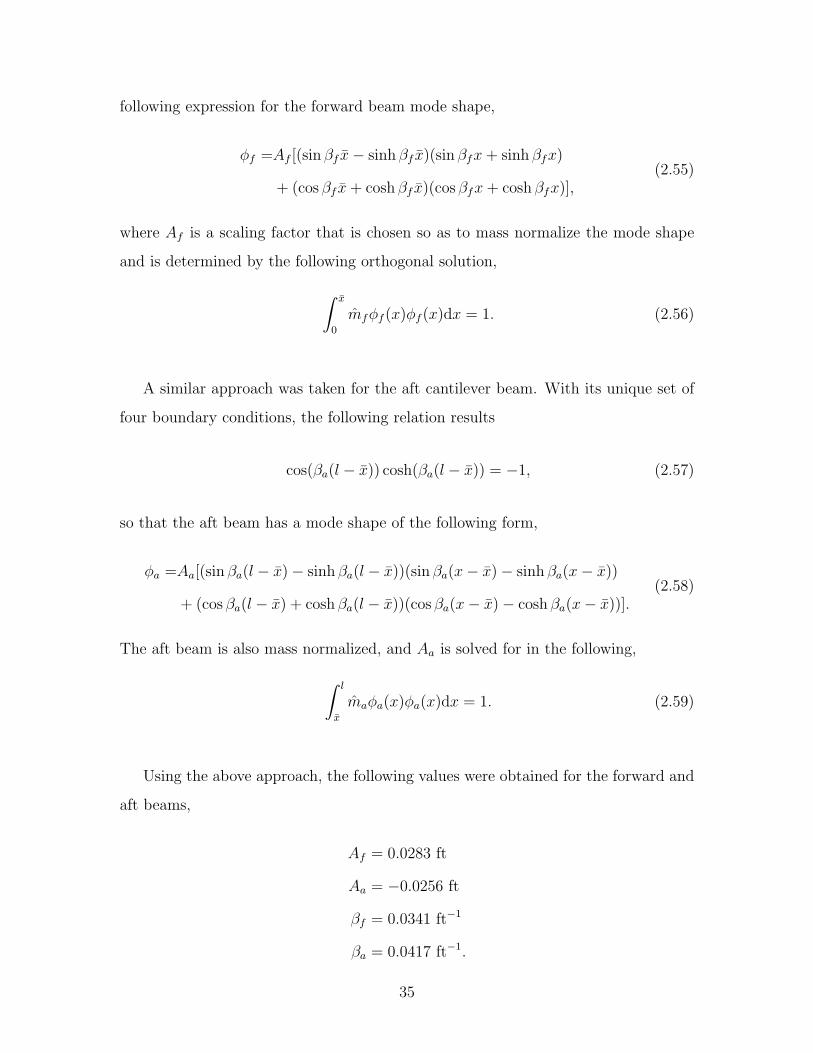
A visual representation of the combined forward and aft mode shapes as described in
(2.55) and (2.58) is shown in Figure 2-7.
0 10 20 30 40 50 60 70 80 90 1000
0.05
0.1
0.15
0.2
distance from nose of HSV [ft]
mod
e sh
ape
φ(x
) [f
t]
Figure 2-7: Forward and aft mode shape.
2.3.2 Forced Modal Response
The forced response associated with (2.44) is of the form,
EI∂4y(x, t)
∂x4+ m
∂2y(x, t)
∂t2= p(x, t) + Pj(x, t)δ(x− xj), (2.60)
where p denotes pressure and P is a point load. The above equation has solutions for
y as,
y(x, t) =∞∑k=1
φk(x)ηk(t). (2.61)
where the infinite summation over k illustrates the fact that there are infinitely many
modes for a fixed–free beam. Do not confuse that with the subscripts f and a. The
discussion thus far has not distinguished between forward and aft, and is of a generic
flavor. The η terms will later be regarded as the flexible state variables, and are
36
governed by the following second order equation
ηk + ω2kηk = Nk(t) (2.62)
where Nk is the modal force defined as,
Nk(t) =
∫φk(x)p(x, t)dx+
l∑j=1
φk(xj)Pj(t). (2.63)
Once again, the flexible model used in this work only pertains to the first bending
modes for each beam. Application of (2.63) to the forward and aft beams results in
the following force relations
Nf (t) =−∫ x
0
φf (x)p(x, t)dx+ (−φf (xc)Fz,c(t)) (2.64)
Na(t) =−∫ l
x
φa(x)p(x, t)dx+ (−φa(xe)Fz,e(t)). (2.65)
Notice the minus signs in the above expression. The flexible beam model coordinate
system denotes up as positive, where as the coordinate system for the rigid–body
dynamics, down is assumed to be positive.
2.4 Equations of Motion
Two distinct aircraft models will be introduced in this study. One aircraft model will
incorporate the flexible effects and will be used for controller evaluation, and as so
will be referred to as the Evaluation Model (EM). The second model will only include
the rigid–body effects and will be used for control design, and will be referred to as
the Evaluation Model (EM). The construction and implementation of those models is
discussed below.
37
2.4.1 Evaluation Model
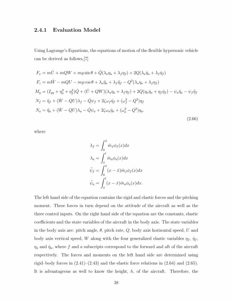
Using Lagrange’s Equations, the equations of motion of the flexible hypersonic vehicle
can be derived as follows,[7]
Fx = mU +mQW +mg sin θ + Q(λaηa + λfηf ) + 2Q(λaηa + λf ηf )
Fz = mW −mQU −mg cos θ + λaηa + λf ηf −Q2(λaηa + λfηf )
My = (Iyy + η2a + η2
f )Q+ (U +QW )(λaηa + λfηf ) + 2Q(ηaηa + ηf ηf )− ψaηa − ψf ηf
Nf = ηf + (W −QU)λf − Qψf + 2ζωf ηf + (ω2f −Q2)ηf
Na = ηa + (W −QU)λa − Qψa + 2ζωaηa + (ω2a −Q2)ηa.
(2.66)
where
λf =
∫ x
0
mfφf (x)dx
λa =
∫ l
x
maφa(x)dx
ψf =
∫ x
0
(x− x)mfφf (x)dx
ψa =
∫ l
x
(x− x)maφa(x)dx.
The left hand side of the equation contains the rigid and elastic forces and the pitching
moment. These forces in turn depend on the attitude of the aircraft as well as the
three control inputs. On the right hand side of the equation are the constants, elastic
coefficients and the state variables of the aircraft in the body axis. The state variables
in the body axis are: pitch angle, θ, pitch rate, Q, body axis horizontal speed, U and
body axis vertical speed, W along with the four generalized elastic variables ηf , ηf ,
ηa and ηa, where f and a subscripts correspond to the forward and aft of the aircraft
respectively. The forces and moments on the left hand side are determined using
rigid–body forces in (2.41)–(2.43) and the elastic force relations in (2.64) and (2.65).
It is advantageous as well to know the height, h, of the aircraft. Therefore, the
38

following kinematic relation,
h = U sin θ −W cos θ (2.67)
is introduced.
The implementation of Equation (2.66) is cumbersome and slow on any computer.
Some of the solutions for obtaining the pressure distribution and subsequent forces
on the hypersonic vehicle require solving nonlinear equations. A more implementable
aircraft model is obtained through the transformation of the above system to the
stability axis and then the subsequent curve fitting of the forces and moments to
that of an algebraic relations. This increases the ease of implantation of the aircraft
model, and greatly reduces computation time. Equation (2.66) can be transformed
to the stability axis with the following coordinate transformation equations,
α = W/U
V 2 = U2 +W 2
V = (UU +WW )/V
α = (UW −WU)/V
(2.68)
where α is the angle of attack and V is the velocity of the HSV. The relationship
between the stability axes variables and body axes variables is illustrated in Figure2-8.
Lx; U
V
θ γ
L; U
Fx; T
DFz
z,W
Upper-sideElevator
Canard
¿1;l
¿1;u
¿2
Upper-side
Aft±c
±e
Canard
xz
Forward
Under-side
ScramjetShear Layer
Bow shock: f(Á)
1
Figure 2-8: Axes of the HSV
39
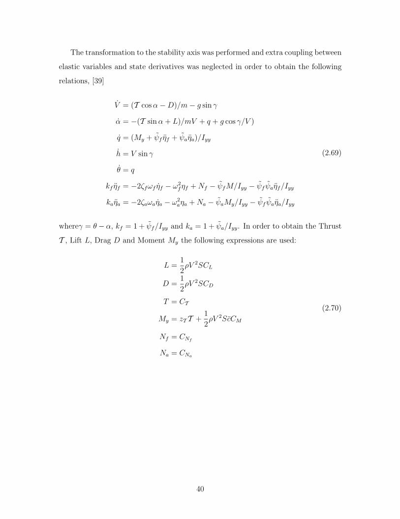
The transformation to the stability axis was performed and extra coupling between
elastic variables and state derivatives was neglected in order to obtain the following
relations, [39]
V = (T cosα−D)/m− g sin γ
α = −(T sinα + L)/mV + q + g cos γ/V )
q = (My + ψf ηf + ψaηa)/Iyy
h = V sin γ
θ = q
kf ηf = −2ζfωf ηf − ω2fηf +Nf − ψfM/Iyy − ψf ψaηf/Iyy
kaηa = −2ζaωaηa − ω2aηa +Na − ψaMy/Iyy − ψf ψaηa/Iyy
(2.69)
whereγ = θ− α, kf = 1 + ψf/Iyy and ka = 1 + ψa/Iyy. In order to obtain the Thrust
T , Lift L, Drag D and Moment My the following expressions are used:
L =1
2ρV 2SCL
D =1
2ρV 2SCD
T = CT
My = zT T +1
2ρV 2ScCM
Nf = CNf
Na = CNa
(2.70)
40
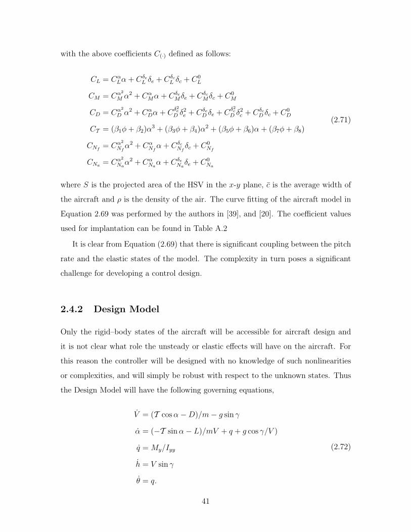
with the above coefficients C(·) defined as follows:
CL = CαLα + Cδe
L δe + CδcL δc + C0
L
CM = Cα2
M α2 + CαMα + Cδe
Mδe + CδcMδc + C0
M
CD = Cα2
D α2 + CαDα + C
δ2eD δ
2e + Cδe
D δe + Cδ2cD δ
2c + Cδc
D δc + C0D
CT = (β1φ+ β2)α3 + (β3φ+ β4)α2 + (β5φ+ β6)α + (β7φ+ β8)
CNf= Cα2
Nfα2 + Cα
Nfα + Cδc
Nfδc + C0
Nf
CNa = Cα2
Naα2 + Cα
Naα + Cδe
Naδe + C0
Na
(2.71)
where S is the projected area of the HSV in the x-y plane, c is the average width of
the aircraft and ρ is the density of the air. The curve fitting of the aircraft model in
Equation 2.69 was performed by the authors in [39], and [20]. The coefficient values
used for implantation can be found in Table A.2
It is clear from Equation (2.69) that there is significant coupling between the pitch
rate and the elastic states of the model. The complexity in turn poses a significant
challenge for developing a control design.
2.4.2 Design Model
Only the rigid–body states of the aircraft will be accessible for aircraft design and
it is not clear what role the unsteady or elastic effects will have on the aircraft. For
this reason the controller will be designed with no knowledge of such nonlinearities
or complexities, and will simply be robust with respect to the unknown states. Thus
the Design Model will have the following governing equations,
V = (T cosα−D)/m− g sin γ
α = (−T sinα− L)/mV + q + g cos γ/V )
q = My/Iyy
h = V sin γ
θ = q.
(2.72)
41
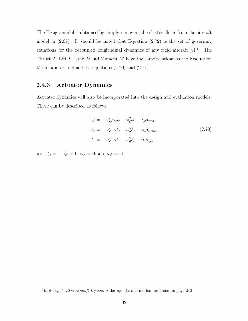
The Design model is obtained by simply removing the elastic effects from the aircraft
model in (2.69). It should be noted that Equation (2.72) is the set of governing
equations for the decoupled longitudinal dynamics of any rigid aircraft.[44]1. The
Thrust T , Lift L, Drag D and Moment M have the same relations as the Evaluation
Model and are defined by Equations (2.70) and (2.71).
2.4.3 Actuator Dynamics
Actuator dynamics will also be incorporated into the design and evaluation models.
These can be described as follows:
φ = −2ζφωφφ− ω2φφ+ ωφφcmd
δe = −2ζδωδδe − ω2δδe + ωδδe,cmd
δc = −2ζδωδδc − ω2δδc + ωδδc,cmd
(2.73)
with ζφ = 1, ζδ = 1, ωφ = 10 and ωδ = 20.
1In Stengel’s 2004 Aircraft Dynamics the equations of motion are found on page 240
42
Chapter 3
Controller Design
The control structure proposed has a combination of feedforward input, nominal
feedback, and adaptive feedback terms. The HSV model is linearized around a desired
trim point. Using the linear model an LQ regulator is then designed. Uncertainties
along with actuator saturation are then introduced and an adaptive control structure
is then explored that adjusts to the model uncertainties and maintains stability even
with the actuator saturation.
3.1 Linear Model
The underlying design model, described by the DM in (2.72) and the actuator dy-
namics in (2.73) can be expressed compactly as a nonlinear model
X = f(X,U), (3.1)
where X is the state vector and U contains the exogenous inputs φcmd and δe,cmd.
In order to facilitate the control design, we linearize these equations to obtain the
following:
xp = Apxp +Bpu+ ε(t), (3.2)
43
where ε is the linearization error, which is assumed to be small,
Ap =∂f(X,U)
∂X
∣∣∣∣X=X0U=U0
, Bp =∂f(X,U)
∂U
∣∣∣∣X=X0U=U0
,
xp = X −X0, and u = U − U0.
(3.3)
The linear state xp contains the perturbation states, [∆V ∆α ∆q ∆h ∆θ ∆φ ∆φ ∆δe ∆δe]T
and u is the command input perturbation vector, [∆φcmd ∆δe,cmd]T.
Integral error states will be augmented to the linear model of the HSV for com-
mand following purposes. The reference command , r, will be given in h − V space
and is constructed as
r = [∆Vref ∆href]T (3.4)
Denoting an output y = [∆V ∆h]T an integral error state eI can be expressed as
eI = ∫(y − r)dτ = ∫(Hxp − r)dτ, (3.5)
where H is a selection matrix. In addition to error augmentation, the actuator inputs
will be explicitly incorporated into the linear model as states, and a new input v is
defined as
v = u. (3.6)
By augmenting both the command following error in (3.5) and actuator inputs in
(3.6) to the linear system in (3.2) the overall system to be controlled becomes,
xp
eI
u
︸ ︷︷ ︸
x
=
Ap 0 Bp
H 0 0
0 0 0
︸ ︷︷ ︸
A
xp
eI
u
︸ ︷︷ ︸
x
+
0
0
I
︸︷︷︸B
v +
0
−I
0
︸ ︷︷ ︸Bcmd
r, (3.7)
which can be compactly expressed as,
x = Ax+Bv +Bcmdr. (3.8)
44
3.2 Baseline Controller
The baseline controller is designed so that HSV will follow a given a reference signal
in h–V . Thus with the given task of y tending to some r at steady state it is clear
that eI will have reached some constant value, so that eI is now zero and with that;
the plant state xp will have reached some ideal x∗p with some ideal input u∗. More
compactly the following expression will be satisfied,0
r
=
Ap Bp
H 0
x∗pu∗
. (3.9)
With the following construction,
G =
Ap Bp
H 0
−1
=
G11 G12
G21 G22
(3.10)
and with some algebra we find that,
x∗p = G12r
u∗ = G22r.(3.11)
We now define,
xp = xp − x∗p
u = u− u∗(3.12)
and collecting terms compactly,
x =[xTp e
T uT]T
(3.13)
45
The linear system of (3.8) can now been cast into that of an LQ regulator of the
following form,1
˙x = Ax+Bv. (3.14)
A linear quadratic cost function is then chosen as
J =
∫(xTQx+ vTRv)dτ, (3.15)
where Q and R are suitably chosen positive definite matrices. For more details per-
taining to the values chosen for Q and R refer to Appendix C. The nominal feedback
gain satisfies the following,
K = argminK
J(v, x, Q,R) | v = KTx
(3.16)
and through the expansion of x the control input in terms of the state varable vectore
x and reference signal r...finsih
v =KTx
=[K1 K2 K3][xTp e
T uT]T
=(−K1G12 −K3G22)r +K1xp +K2e+K3u
=Kffr +KTx
(3.17)
Noting that the components of x include the integral eI , and u it follows that the
baseline controller has Proportional, Integral, and Filter components, thus, leading
to a PIF-LQ regulator as first introduced in [42] with more details given in [43] and
[44]. The PIF control structure is shown in Figures 3-1 and 3-2.
1The construction of x is covered in great detail in Reference [43] page 523 and PIF controlstructure on pages 528-531.
46
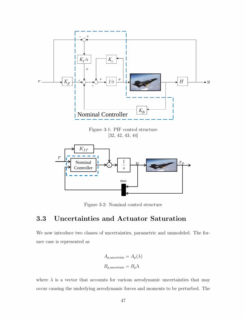
Nominal Controller
Figure 3-1: PIF control structure[32, 42, 43, 44]
Nominal +
ru xp
Controller + p
mux
Figure 3-2: Nominal control structure
3.3 Uncertainties and Actuator Saturation
We now introduce two classes of uncertainties, parametric and unmodeled. The for-
mer case is represented as
Ap,uncertain = Ap(λ)
Bp,uncertain = BpΛ
where λ is a vector that accounts for various aerodynamic uncertainties that may
occur causing the underlying aerodynamic forces and moments to be perturbed. The
47
specific construction of λ is shown,
λ =[λm λL λM λCG
]Twhere:
• λm: Multiplicative uncertainty in the inertial properties, m = λmm0, and Iyy =
λmIyy,0 where
• λL: Multiplicative uncertainty in lift, CαL = λLC
αL,0.
• λM : Multiplicative uncertainty in pitching moment, CαM = λMCM,0.
• λCG: Longitudinal distance between the neutral point and the center of gravity.
This distance divided by the mean aerodynamic chord will be denoted as λCG.
While a negative value of λCG denotes that the CG has been moved backwards,
positive values denote a forward CG movement.
Capital lambda, Λ, is a 2x2 diagonal matrix that represents uncertainties in the
actuator that may occur due to damages or failures, leading to loss of effectiveness.
Unmodeled uncertainties include the flexible effects, which are neglected in the
design model, as well as time-delays, such as computational lags. If the unmod-
eled uncertainties and linearization errors are neglected, the underlying plant can be
expressed as
xp = Ap(λ)xp +BpΛu. (3.18)
In addition to the above uncertainties, our studies also include magnitude saturation
in the actuators. This is accounted for with the inclusion of a rectangular saturation
function Rs(u) where the i–th component is defined as, [28]
Rsi=
ui if umini
≤ ui ≤ umaxi,
umaxiif ui > umaxi
,
uminiif ui < umini
(3.19)
48
for i = 1, 2.
A visual representation of the uncertainties and saturation effects is shown in Figure
3-3.
Saturation
ΛActuator Failure\
τTime Delay
λUncertaintyy
λ , PlantUncertainty
Figure 3-3: Uncertainty modelling
3.4 Adaptive Controller
In order to compensate for the modeling uncertainties, an adaptive controller is now
added to the baseline controller described in Section A. We note that the adaptive
controller is designed to directly accommodate the parametric uncertainties while it
is designed so as to be robust with respect to the unmodeled uncertainties. The
structure of this adaptive controller is chosen as
v =
baseline︷ ︸︸ ︷Kffr + KTx︸︷︷︸
nominal
+ θ(t)Tx︸ ︷︷ ︸adaptive
(3.20)
The adaptive component of the controller is denoted, θ, as can be seen in (3.20) and
has the same dimension as the nominal feedback gain K. The adaptive component
augments naturally with the nominal controller and a visual interpretation of this
can be seen in Figure 3-4.
Combining the uncertain plant model in ??eq:plantuncert) with the integral state
eI in (3.5), the input-state in ??eq:inputder), the the saturation function in (3.19), and
the overall baseline and adaptive control input from (3.20), the closed loop equations
49
Nominal Controller +
ru
Λ τ xp
Adaptive Controller
Saturation Actuator Failure\Uncertainty
Time Delay
λ , PlantUncertainty
mux
Figure 3-4: Nominal with adaptive augmentation and uncertainty
are given by, xp
e
u
︸ ︷︷ ︸
x
=
Ap(λ) 0 BpΛ
H 0 0
K1 + θ1(t) K2 + θ2(t) K3 + θ3(t)
︸ ︷︷ ︸
A(λ,Λ)+B(KT+θ(t)T)
xp
e
u
︸ ︷︷ ︸
x
+
0
−I
0
︸ ︷︷ ︸Bcmd
Kffr −
Bp
0
0
︸ ︷︷ ︸B1
Λu∆,
(3.21)
where u∆ = u−Rs(u), and in compact form reduces to,
x = (A(λ,Λ) +B(KT + θ(t)T))x+BcmdKffr −B1Λu∆. (3.22)
A reference model is chosen as
xm = Amxm −Bmr. (3.23)
where Am and Bm are such that Am is a Hurwitz matrix, Bm = BcmdKff and ∆Am =
A(λ,Λ) + B(KT + θ∗T) − Am is arbitrarily small. We note that due to the addition
of the integral action, it may not be possible to choose ∆Am to be zero for general
50
parametric uncertainties. Defining the state error e as,
e = x− xm, (3.24)
Design Methodology: Incorporating Saturation
Reference Model
u
Σ-
xm
e
Saturation
Σ
+xR(u)
Σ
Reference Model
-+
u¢
Σ
e¢
-
+eu
Modelu¢ ¢
_µ ¡ x eTPB sign(¤) ¾ µµ = ¡¡µxaugeuPB1sign(¤)¡ ¾µµ
_Kc = ¡¡cxgceTuPB1sign(¤)¡ ¾cKc
_d = ¡¡dsign(¤)BT1 Peu ¡ ¾dd
13
_¸ = ¡¡¸diag(u¢)BT
1 Peu ¡ ¾¸¸
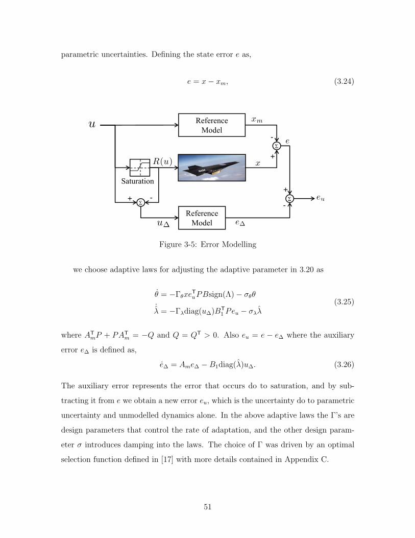
Figure 3-5: Error Modelling
we choose adaptive laws for adjusting the adaptive parameter in 3.20 as
θ = −ΓθxeTuPBsign(Λ)− σθθ
˙λ = −Γλdiag(u∆)BT
1 Peu − σλλ(3.25)
where ATmP + PAT
m = −Q and Q = QT > 0. Also eu = e − e∆ where the auxiliary
error e∆ is defined as,
e∆ = Ame∆ −B1diag(λ)u∆. (3.26)
The auxiliary error represents the error that occurs do to saturation, and by sub-
tracting it from e we obtain a new error eu, which is the uncertainty do to parametric
uncertainty and unmodelled dynamics alone. In the above adaptive laws the Γ’s are
design parameters that control the rate of adaptation, and the other design param-
eter σ introduces damping into the laws. The choice of Γ was driven by an optimal
selection function defined in [17] with more details contained in Appendix C.
51

52
Chapter 4
Simulation Studies
In order to assess the robustness of the adaptive control scheme, several simulation
studies were performed. In the simulation studies the adaptive controller is compared
to the nominal controller under an uncertain plant flight condition. All of the simu-
lation begin with the HSV Evaluation Model in level flight at an altitude of 85,000
ft and travelling at Mach 8. The trim values for the HSV at this flight condition are
given in Table A.3.
Table 4.1: Trim values for two input HSV model.
State Variable Trim Value Units
V 7850 ft/sα 0.0268 radq 0 rad/sh 85000 ftθ 0.0268 radηf 0.939 –ηf 0 –ηa 0.775 –ηa 0 –
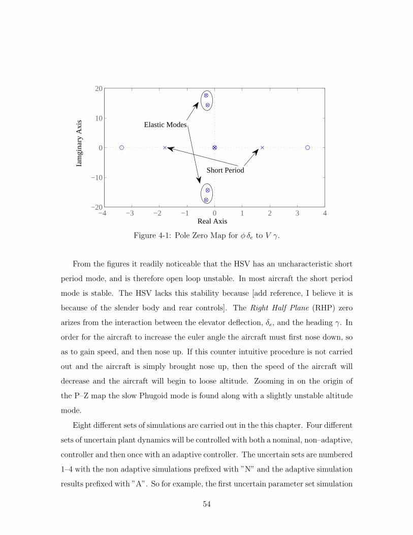
Using a similar approach to that shown in Equation (3.3) was performed on the
Evaluation Model. Using the state Jacobian and the input Jacobian matrices a pole–
zero plot of the transfer matrix from the control inputs φ and δe to V and γ was
generated and is shown in Figure 4-1, with a zoom of the origin shown in Figure 4-2.
53
Real Axis
Iam
gina
ry A
xis
−4 −3 −2 −1 0 1 2 3 4−20
−10
0
10
20
Elastic Modes
Short Period
Figure 4-1: Pole Zero Map for φ δe to V γ.
From the figures it readily noticeable that the HSV has an uncharacteristic short
period mode, and is therefore open loop unstable. In most aircraft the short period
mode is stable. The HSV lacks this stability because [add reference, I believe it is
because of the slender body and rear controls]. The Right Half Plane (RHP) zero
arizes from the interaction between the elevator deflection, δe, and the heading γ. In
order for the aircraft to increase the euler angle the aircraft must first nose down, so
as to gain speed, and then nose up. If this counter intuitive procedure is not carried
out and the aircraft is simply brought nose up, then the speed of the aircraft will
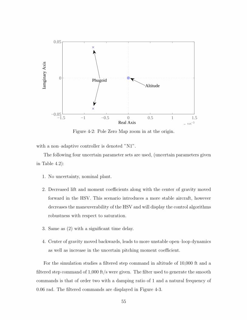
decrease and the aircraft will begin to loose altitude. Zooming in on the origin of
the P–Z map the slow Phugoid mode is found along with a slightly unstable altitude
mode.
Eight different sets of simulations are carried out in the this chapter. Four different
sets of uncertain plant dynamics will be controlled with both a nominal, non–adaptive,
controller and then once with an adaptive controller. The uncertain sets are numbered
1–4 with the non adaptive simulations prefixed with ”N” and the adaptive simulation
results prefixed with ”A”. So for example, the first uncertain parameter set simulation
54
Real Axis
Iam
gina
ry A
xis
−1.5 −1 −0.5 0 0.5 1 1.5
x 10−3
−0.05
0
0.05
PhugoidAltitude
Figure 4-2: Pole Zero Map zoom in at the origin.
with a non–adaptive controller is denoted ”N1”.
The following four uncertain parameter sets are used, (uncertain parameters given
in Table 4.2):
1. No uncertainty, nominal plant.
2. Decreased lift and moment coefficients along with the center of gravity moved
forward in the HSV. This scenario introduces a more stable aircraft, however
decreases the maneuverability of the HSV and will display the control algorithms
robustness with respect to saturation.
3. Same as (2) with a significant time delay.
4. Center of gravity moved backwards, leads to more unstable open–loop dynamics
as well as increase in the uncertain pitching moment coefficient.
For the simulation studies a filtered step command in altitude of 10,000 ft and a
filtered step command of 1,000 ft/s were given. The filter used to generate the smooth
commands is that of order two with a damping ratio of 1 and a natural frequency of
0.06 rad. The filtered commands are displayed in Figure 4-3.
55
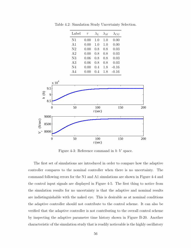
Table 4.2: Simulation Study Uncertainty Selection.
Label τ λL λM λCG
N1 0.00 1.0 1.0 0.00A1 0.00 1.0 1.0 0.00N2 0.00 0.8 0.8 0.03A2 0.00 0.8 0.8 0.03N3 0.06 0.8 0.8 0.03A3 0.06 0.8 0.8 0.03N4 0.00 0.4 1.8 -0.16A4 0.00 0.4 1.8 -0.16
0 50 100 150 200
8000
8500
9000
Vt
(ft/s
ec)
t (sec)
0 50 100 150 200
8.5
9
9.5
x 104
h (
ft)
t (sec)
Figure 4-3: Reference command in h–V space.
The first set of simulations are introduced in order to compare how the adaptive
controller compares to the nominal controller when there is no uncertainty. The
command following errors for the N1 and A1 simulations are shown in Figure 4-4 and
the control input signals are displayed in Figure 4-5. The first thing to notice from
the simulation results for no uncertainty is that the adaptive and nominal results
are indistinguishable with the naked eye. This is desirable as at nominal conditions
the adaptive controller should not contribute to the control scheme. It can also be
verified that the adaptive controller is not contributing to the overall control scheme
by inspecting the adaptive parameter time history shown in Figure B-20. Another
characteristic of the simulation study that is readily noticeable is the highly oscillatory
56
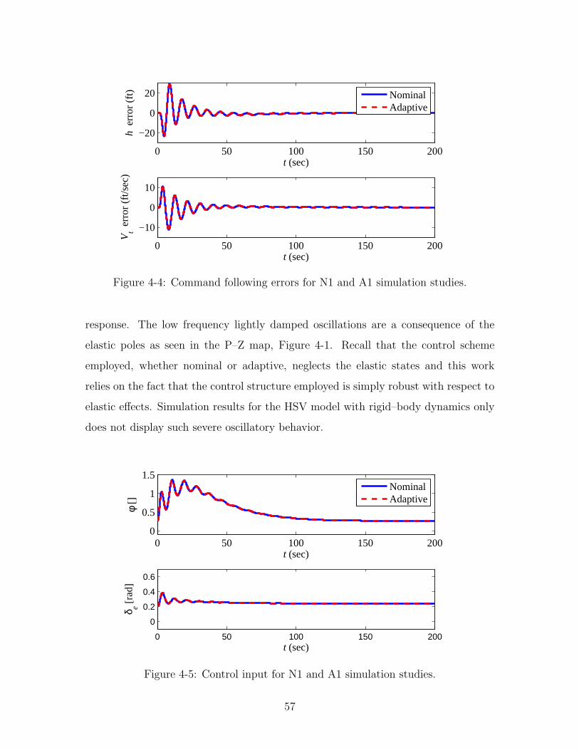
0 50 100 150 200
−10
0
10
Vt e
rror
(ft/
sec)
t (sec)
0 50 100 150 200
−20
0
20
h e
rror
(ft)
t (sec)
NominalAdaptive
Figure 4-4: Command following errors for N1 and A1 simulation studies.
response. The low frequency lightly damped oscillations are a consequence of the
elastic poles as seen in the P–Z map, Figure 4-1. Recall that the control scheme
employed, whether nominal or adaptive, neglects the elastic states and this work
relies on the fact that the control structure employed is simply robust with respect to
elastic effects. Simulation results for the HSV model with rigid–body dynamics only
does not display such severe oscillatory behavior.
0 50 100 150 2000
0.5
1
1.5
φ []
t (sec)
NominalAdaptive
0 50 100 150 200
0
0.2
0.4
0.6
δ e [ra
d]
t (sec)
Figure 4-5: Control input for N1 and A1 simulation studies.
57
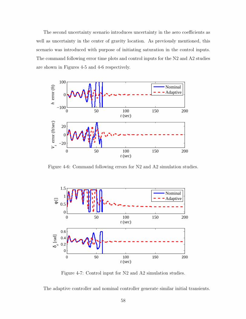
The second uncertainty scenario introduces uncertainty in the aero coefficients as
well as uncertainty in the center of gravity location. As previously mentioned, this
scenario was introduced with purpose of initiating saturation in the control inputs.
The command following error time plots and control inputs for the N2 and A2 studies
are shown in Figures 4-5 and 4-6 respectively.
0 50 100 150 200
−20
0
20
Vt e
rror
(ft/
sec)
t (sec)
0 50 100 150 200−100
0
100
h e
rror
(ft)
t (sec)
NominalAdaptive
Figure 4-6: Command following errors for N2 and A2 simulation studies.
0 50 100 150 2000
0.5
1
1.5
φ []
t (sec)
NominalAdaptive
0 50 100 150 200
0
0.2
0.4
0.6
δ e [ra
d]
t (sec)
Figure 4-7: Control input for N2 and A2 simulation studies.
The adaptive controller and nominal controller generate similar initial transients.
58
However, as time progresses the adaptive control results limit cycle for shorter and
shorter periods of time, while the nominal controller limit cycles until the angle of
attack departs severely and the simulation is stopped. The adaptive parameters, as
seen in Figure ??, adjust in a stable fashion even during saturation because of the use
of the augmented error dynamics eu as shown in Figure (3-5). If the generic reference
model error e were used instead of eu the adaptive controller would not perform as
well during saturation.
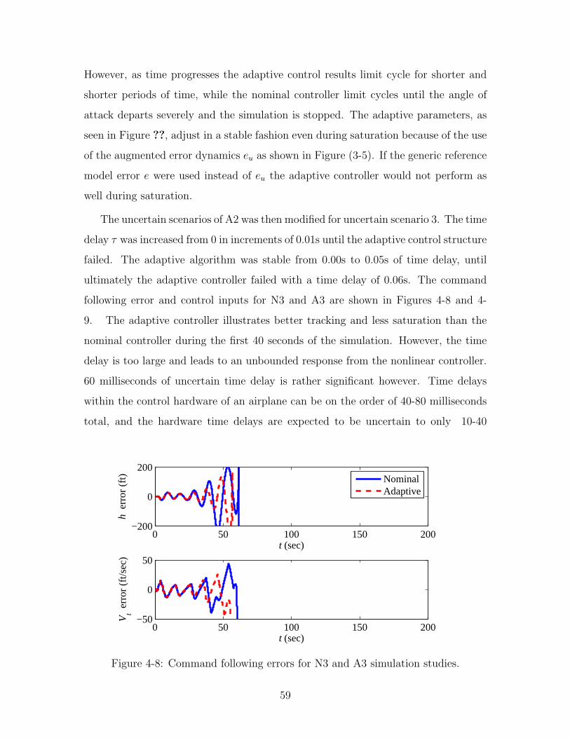
The uncertain scenarios of A2 was then modified for uncertain scenario 3. The time
delay τ was increased from 0 in increments of 0.01s until the adaptive control structure
failed. The adaptive algorithm was stable from 0.00s to 0.05s of time delay, until
ultimately the adaptive controller failed with a time delay of 0.06s. The command
following error and control inputs for N3 and A3 are shown in Figures 4-8 and 4-
9. The adaptive controller illustrates better tracking and less saturation than the
nominal controller during the first 40 seconds of the simulation. However, the time
delay is too large and leads to an unbounded response from the nonlinear controller.
60 milliseconds of uncertain time delay is rather significant however. Time delays
within the control hardware of an airplane can be on the order of 40-80 milliseconds
total, and the hardware time delays are expected to be uncertain to only 10-40
0 50 100 150 200−50
0
50
Vt e
rror
(ft/
sec)
t (sec)
0 50 100 150 200−200
0
200
h e
rror
(ft)
t (sec)
NominalAdaptive
Figure 4-8: Command following errors for N3 and A3 simulation studies.
59
0 50 100 150 2000
0.5
1
1.5
φ []
t (sec)
NominalAdaptive
0 50 100 150 200
0
0.2
0.4
0.6
δ e [ra
d]
t (sec)
Figure 4-9: Control input for N3 and A3 simulation studies.
milliseconds. When time delays are known they can be incorporated into the reference
model, leaving only the uncertain component of the delay as parasitic . [make better,
its late, reference my work at NASA]
The last uncertainty scheme introduces and obscure scenario. The uncertain pa-
rameters are rather large, in fact larger than they are in scenario 2. Yet the adaptive
controller and nominal controller results are indistinguishable. The command follow-
ing error and control inputs for N3 and A3 are shown in Figures ?? and ??. The
0 50 100 150 200−20
0
20
Vt e
rror
(ft/
sec)
t (sec)
0 50 100 150 200−40
−20
0
20
40
h e
rror
(ft)
t (sec)
NominalAdaptive
Figure 4-10: Command following errors for N4 and A4 simulation studies.
60
0 50 100 150 2000
0.5
1
1.5
φ []
t (sec)
NominalAdaptive
0 50 100 150 200
0
0.2
0.4
0.6
δ e [ra
d]
t (sec)
Figure 4-11: Control input for N4 and A4 simulation studies.
simple fact of the matter is that the command following error was not large enough
to instigate changes in the adaptive parameter, see Figure B-40. This leads to the
idea that uncertainty in the parameter space does not map intuitively to the failure
or success of the adaptive or non adaptive results. Therefore its difficult to assess
the overall performance of the adaptive algorithm. This leads to Chapter 5. Where
a more rigorous approach at controller validation is performed.[poor sentences]
61

62
Chapter 5
Control Verification, A different
Approach
In order to have a better assessment of the improvement in performance with the
adaptive controller, we use tools that have been developed in [16] and [15] . In order
to make the exposition self contained, the tools developed in [16] and [15] are briefly
explained below.
5.1 Mathematical Framework
The parameters which specify the closed-loop system are grouped into two categories:
uncertain parameters which are denoted by the vector p, and the control design
parameters which are denoted by the vector d. While the plant model depends on
p, the controller depends on d. The Nominal Parameter value, denoted as p, is a
deterministic estimate of the true value of p. Stability and performance requirements
for the closed-loop system will be prescribed by the set of inequality constraints
g(p, d) < 0. For a fixed d, the larger the region in p-space where g < 0 the more robust
the controller. The Failure Domain corresponding to the controller with parameter d
63
is given by1
F j(d) = p : gj(p, d) ≥ 0, (5.1)
F(d) =
dim(g)⋃j=1
F j(d). (5.2)
While Equation (5.1) describes the failure domain corresponding to the jth require-
ment, Equation (5.2) describes the failure domain for all requirements. The Non-
Failure Domain is the complement set of the failure domain and will be denoted2 as
F c. The names “failure domain” and “non-failure domain” are used because in the
failure domain at least one constraint is violated while, in the non-failure domain, all
constraints are satisfied.
Let a reference set where the parameter p lies be given by the hyper-rectangle,
R(p, n) = p : p− n ≤ p ≤ p+ n . (5.3)
where n > 0 is the vector of half-lengths. One of the tasks of interest is to assign a
measure of robustness to a controller based on measuring how much the reference set
can be deformed before intersecting the failure domain.
In what follows we assume that g(p, d) < 0. We define a Critical Parameter Value,
CPV, as the point where the deforming set touches the failure domain. The CPV
corresponding to the deformation of R(p, n) for the jth requirement is given by
pj = argminp‖p− p‖∞n : gj(p, d) ≥ 0, Ap ≥ b , (5.4)
where ‖x‖∞n = supi|xi|/ni is the n-scaled infinity norm. The last constraint is
used to exclude regions of the parameter space where plants are infeasible and/or
uncertainty levels are unrealistic. The overall CPV is
p = pk, (5.5)
1Throughout this paper, super-indices are used to denote a particular vector or set while numericalsub-indices refer to vector components, e.g., pj
i is the ith component of the vector pj .2The complement set operator will be denoted as the super-index c.
64
where
k = argmin1≤j≤dim(g)
‖pj − p‖∞n
. (5.6)
Hence, once the CPV for each individual constraint function is solved for, the overall
CPV is the closest of these CPVs to the nominal parameter point according to the
n-scaled infinity norm.
The size of the deformed set is proportional to Rectangular PSM, which is defined
as
ρ = α‖n‖, (5.7)
where α = ‖p − p‖∞n , referred to as the critical similitude ratio, is non-dimensional,
but depends on both the shape and the size of the reference set.[14] The PSM has
the same units as the uncertain parameters, and depends on the shape, but not the
size, of the reference set. If the PSM is zero, the controller’s robustness is practically
nil since there are infinitely small perturbations of p leading to the violation of at
least one of the requirements. If the PSM is positive, the requirements are satisfied
for parameter points in the vicinity of the the nominal parameter point. The larger
the PSM, the larger the hyper-rectangular vicinity.
5.2 Hypersonic Vehicle Uncertainty
The following uncertain parameters will be considered in subsequent analysis
1. Multiplicative uncertainty in the inertial properties: λm ∈ (0, 2].
2. Multiplicative uncertainty in lift: λL ∈ (0, 2].
3. Multiplicative uncertainty in pitching moment: λM ∈ (0, 2].
4. Time delay τ in both plant inputs, where τ ∈ (0, 0.04].
5. Longitudinal distance between the neutral point and the center of gravity λCG ∈
[−0.1, 0.1].
65
The reference set Ω for p = [λm, λL, λM , τ, λCG] to be used is a hyper-rectangle with
aspect vector n = [1, 1, 1, 0.04, 0.1] and nominal parameter point p = [1, 1, 1, 0, 0].
Note that n determines the relative levels of uncertainty among parameters, e.g.,
there is 0.04/0.1 more uncertainty in the CG location than in the time delay.
A set of closed-loop requirements is introduced subsequently. Lets define the
vector of signals
h(p, d, t) =[V (p, d, t)− 10g, |α(p, d, t)| − 0.2, (5.8)
‖eI,1(p, d, t)‖2 − q‖eI,1(p, dbase, tf )‖2, (5.9)
‖eI,2(p, d, t)‖2 − q‖eI,2(p, dbase, tf )‖2], (5.10)
where eI,1 is the velocity error, eI,2 is the altitude error, q is a real number larger than
one, dbase refers to the baseline controller, and tf is a sufficiently large integration
time. This vector enables the formulation of the following set of requirements:
1. Structural: the load factor must not exceed 10, i.e., g1 = maxth1.
2. Stability and engine stall: the angle of attack must stay in the ±0.2 rad range,
i.e., g2 = maxth2.
3. Tracking performance in velocity: the tracking error must not exceed a pre-
scribed upper bound, i.e., g3 = h3(t = tf ).
4. Tracking performance in altitude: the tracking error must not exceed a pre-
scribed upper bound, i.e., g4 = h4(t = tf ).
In the studies that follow we will evaluate the robustness characteristics of both
controllers for several subsets of [λm, λL, λM , τ, λCG]. Parametric studies indicate
that the trim-ability condition maxumax−U0, U0−umin, where f(X0, U0, p) = 0 for
the saturation limits umax and umin, is satisfied for all the values of p in the range of
interest.
66
5.3 Baseline Controller Analysis
Table 5.1 provides the CPVs corresponding to each individual uncertain parameter for
the baseline controller. The critical requirement corresponding to λm, λL, λM , τ , and
λCG, are g4, g2, g1, g1, and g4 respectively. Note that λCG is the critical parameter and
g4 its most critical requirement. The PSM and the CPV corresponding to p = [τ, λCG]
are equal to ρ = 0.02564 and p = [0.0095,−0.02381]. As with the 1-dimensional case,
the critical requirement is g1. In the case where p = [λm, λL, λM , τ, λCG], the PSM,
the CPV and the critical requirement are ρ = 0.150, p = [1.086, 0.913, 0.962, 8.4 ×
10−11,−0.0086] and g4.
Table 5.1: 1-dimensional CPVs for dbase.
p1 p2 p3 p4
p = [λm] 1.1847 1.1847 1.1845 1.1843
p = [λL] 0.5187 0.5184 0.6540 0.7036
p = [λM ] 0.3670 0.3670 0.3897 0.4015
p = [τ ] 0.0310 ∅ 0.0362 0.0362
p = [λCG] −0.0246 −0.0246 −0.0242 −0.0240
5.4 Adaptive Controller Analysis
Table 5.2 shows the 1-dimensional CPVs associated with the adaptive controller.
The critical requirements corresponding to λm, λL, λM , τ , and λCG, are now g1, g4,
g4, g1, and g4. This set of critical requirements differs from that of the baseline.
As before, the critical parameter is λCG and its most critical requirement g4. The
PSM and the CPV corresponding to p = [τ, λCG] are equal to ρ = 0.02845 and
p = [0.0090,−0.0264]. As with the 1-dimensional case, the critical requirement is
g4. In the case where p = [λm, λL, λM , τ, λCG], the PSM, the CPV and the critical
requirement are ρ = 0.145, p = [1.083, 0.916, 0.963, 8.1× 10⁻¹¹,−0.009] and g4.
67
Table 5.2: 1-dimensional CPVs for dadaptive.
p1 p2 p3 p4
p = [λm] 0.7674 1.2347 0.7643 0.7610
p = [λL] 0.4606 0.4606 0.6005 0.6866
p = [λM ] 0.2271 0.2271 0.2865 0.3629
p = [τ ] 0.0300 0.0316 0.0312 0.0312
p = [λCG] −0.0293 −0.0293 −0.0286 −0.0267
5.5 Comparative Analysis
The improvements in robustness resulting from augmenting the baseline controller
are shown in Table 5.3. The data in Tables 5.1 and 5.2 fully determine Table 5.3.
The adaptive controller attains better margins in the λm, λL, λM , and λCG directions.
While the λm direction leads to the largest improvement, τ produces the only drop.
This situation illustrates the tight dependence that exists between any robust control
assessment method and the uncertainty model assumed. Note that the critical pa-
rameters and the critical requirements corresponding to dbase coincide with those of
dadaptive. Overall the augmented control architecture attains sizable improvements in
all but one of the cases. Since multi-dimensional cases are more realistic, the adoption
of the adaptive controller is well justified.
Table 5.3: Relative PSM improvement.(ρadaptive
ρbaseline− 1)
100%
p = [λm] 26.2%
p = [λL] 5.7%
p = [λM ] 6.5%
p = [τ ] −3.2%
p = [λCG] 11.2%
p = [τ, λCG] 7.7%
p = [λm, λL, λM , τ, λCG] 8.2%
The parameter space p = [τ, l] for the adaptive controller is shown in Figure 5-1.
The non-failure domain, which contains the nominal parameter point, is colored in
68
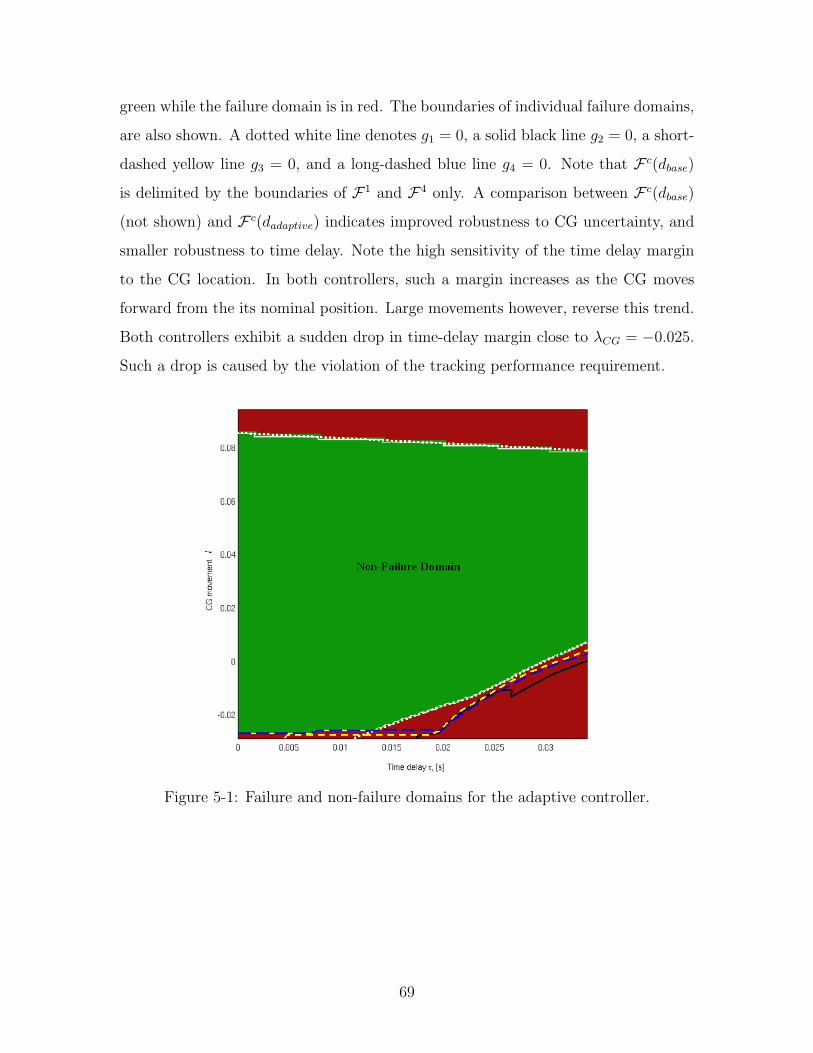
green while the failure domain is in red. The boundaries of individual failure domains,
are also shown. A dotted white line denotes g1 = 0, a solid black line g2 = 0, a short-
dashed yellow line g3 = 0, and a long-dashed blue line g4 = 0. Note that F c(dbase)
is delimited by the boundaries of F1 and F4 only. A comparison between F c(dbase)
(not shown) and F c(dadaptive) indicates improved robustness to CG uncertainty, and
smaller robustness to time delay. Note the high sensitivity of the time delay margin
to the CG location. In both controllers, such a margin increases as the CG moves
forward from the its nominal position. Large movements however, reverse this trend.
Both controllers exhibit a sudden drop in time-delay margin close to λCG = −0.025.
Such a drop is caused by the violation of the tracking performance requirement.
Figure 5-1: Failure and non-failure domains for the adaptive controller.
69

70
Chapter 6
Conclusions
An adaptive controller is proposed for a hypersonic cruise vehicle subject to aerody-
namic uncertainties, center–of– gravity movements, actuator saturation and failures,
and time-delays. The control design is evaluated using a highfidelity HSV model that
considers structural flexibility and thrust-pitch coupling. An elaborate analysis of the
proposed Adaptive Robust Controller for Hypersonic Vehicles (ARCH) is carried out
using a stand-alone control verification methodology. This analysis indicates sizable
improvements in robust performance resulting from adding an adaptive component
to the baseline controller. With the exception of the time-delay margin, where a
slight drop in robustness takes place, the region of safe performance was enlarged
in all other one–dimensional and multi–dimensional directions of the uncertain space
considered. This is particularly remarkable since the parameters and architecture of
the adaptive controller were not tailored according to the closed-loop requirements.
71

72
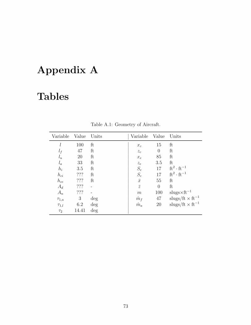
Appendix A
Tables
Table A.1: Geometry of Aircraft.
Variable Value Units Variable Value Units
l 100 ft xc 15 ftlf 47 ft zc 0 ftlu 20 ft xe 85 ftla 33 ft ze 3.5 fthi 3.5 ft Se 17 ft2 · ft−1
hci ??? ft Sc 17 ft2 · ft−1
hce ??? ft x 55 ftAd ??? - z 0 ftAn ??? - m 100 slugs×ft−1
τ1,u 3 deg mf 47 slugs/ft× ft−1
τ1,l 6.2 deg ma 20 slugs/ft× ft−1
τ2 14.41 deg
73
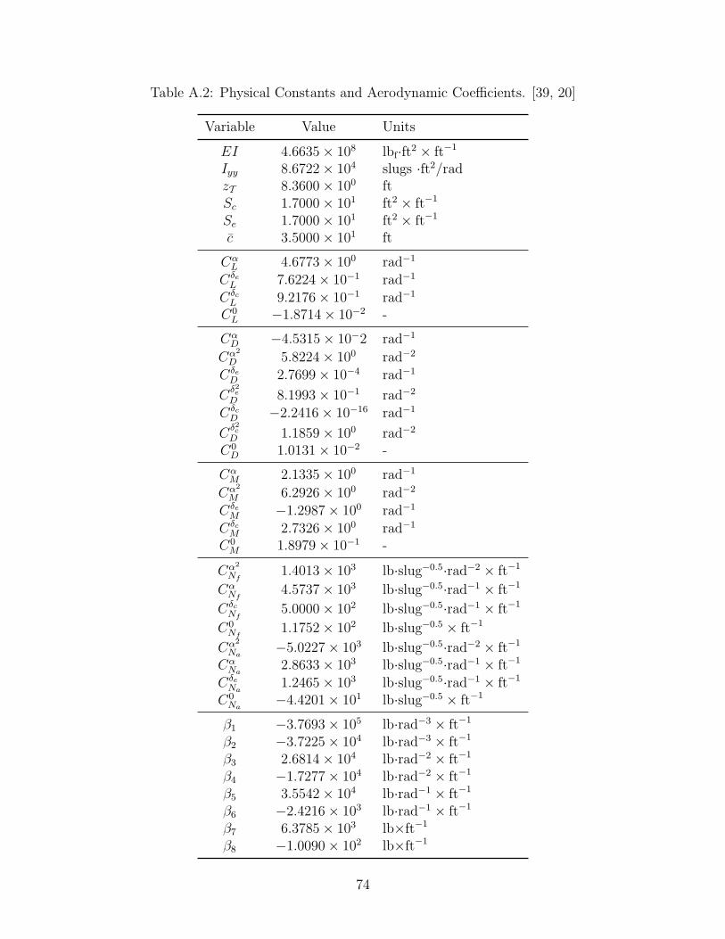
Table A.2: Physical Constants and Aerodynamic Coefficients. [39, 20]
Variable Value Units
EI 4.6635× 10⁸ lbf·ft2 × ft−1
Iyy 8.6722× 10⁴ slugs ·ft2/radzT 8.3600× 100 ftSc 1.7000× 101 ft2 × ft−1
Se 1.7000× 101 ft2 × ft−1
c 3.5000× 101 ft
CαL 4.6773× 100 rad−1
CδeL 7.6224× 10⁻¹ rad−1
CδcL 9.2176× 10⁻¹ rad−1
C0L −1.8714× 10⁻² -
CαD −4.5315× 10⁻² rad−1
Cα2
D 5.8224× 100 rad−2
CδeD 2.7699× 10⁻⁴ rad−1
Cδ2eD 8.1993× 10⁻¹ rad−2
CδcD −2.2416× 10⁻¹⁶ rad−1
Cδ2cD 1.1859× 100 rad−2
C0D 1.0131× 10⁻² -
CαM 2.1335× 100 rad−1
Cα2
M 6.2926× 100 rad−2
CδeM −1.2987× 100 rad−1
CδcM 2.7326× 100 rad−1
C0M 1.8979× 10⁻¹ -
Cα2
Nf1.4013× 103 lb·slug−0.5·rad−2 × ft−1
CαNf
4.5737× 10³ lb·slug−0.5·rad−1 × ft−1
CδcNf
5.0000× 10² lb·slug−0.5·rad−1 × ft−1
C0Nf
1.1752× 10² lb·slug−0.5 × ft−1
Cα2
Na−5.0227× 10³ lb·slug−0.5·rad−2 × ft−1
CαNa
2.8633× 10³ lb·slug−0.5·rad−1 × ft−1
CδeNa
1.2465× 10³ lb·slug−0.5·rad−1 × ft−1
C0Na
−4.4201× 101 lb·slug−0.5 × ft−1
β1 −3.7693× 10⁵ lb·rad−3 × ft−1
β2 −3.7225× 10⁴ lb·rad−3 × ft−1
β3 2.6814× 10⁴ lb·rad−2 × ft−1
β4 −1.7277× 10⁴ lb·rad−2 × ft−1
β5 3.5542× 10⁴ lb·rad−1 × ft−1
β6 −2.4216× 10³ lb·rad−1 × ft−1
β7 6.3785× 10³ lb×ft−1
β8 −1.0090× 10² lb×ft−1
74
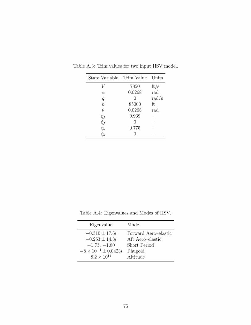
Table A.3: Trim values for two input HSV model.
State Variable Trim Value Units
V 7850 ft/sα 0.0268 radq 0 rad/sh 85000 ftθ 0.0268 radηf 0.939 –ηf 0 –ηa 0.775 –ηa 0 –
Table A.4: Eigenvalues and Modes of HSV.
Eigenvalue Mode
−0.310± 17.6i Forward Aero–elastic−0.253± 14.3i Aft Aero–elastic+1.73, −1.80 Short Period
−8× 10⁻⁴ ± 0.0423i Phugoid8.2× 1014 Altitude
75

76

Appendix B
Figures
77
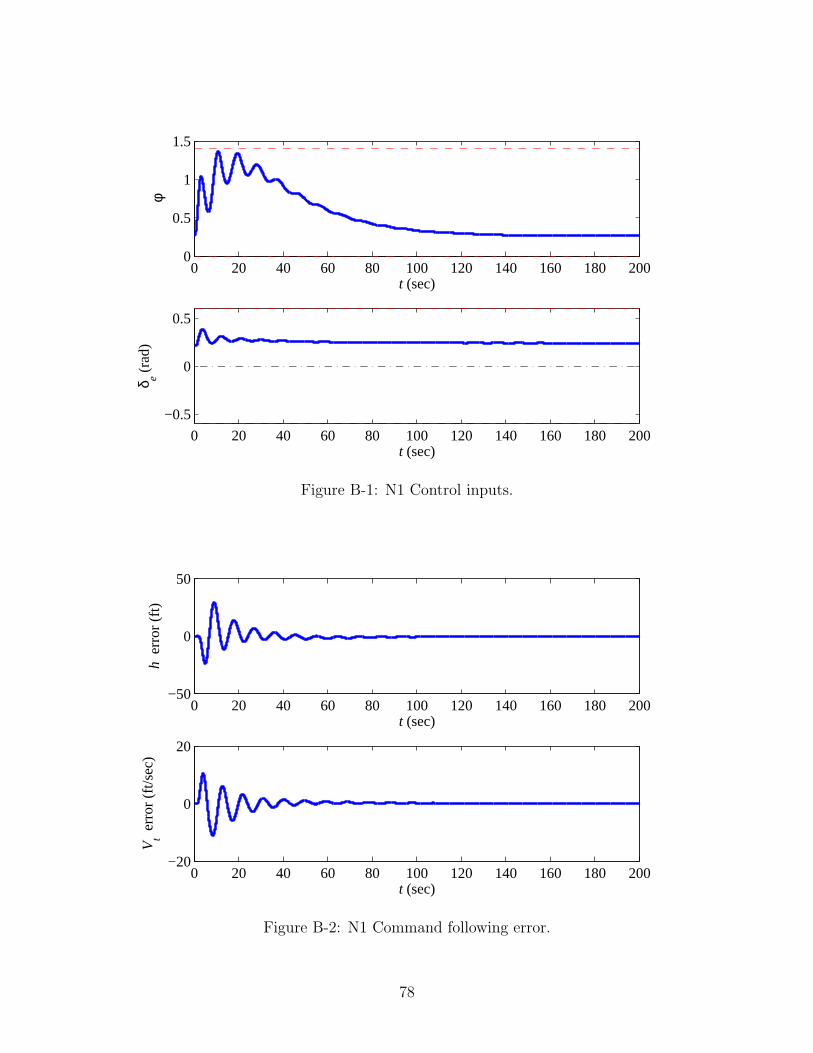
0 20 40 60 80 100 120 140 160 180 2000
0.5
1
1.5φ
t (sec)
0 20 40 60 80 100 120 140 160 180 200
−0.5
0
0.5
δ e (ra
d)
t (sec)
Figure B-1: N1 Control inputs.
0 20 40 60 80 100 120 140 160 180 200−20
0
20
Vt e
rror
(ft/
sec)
t (sec)
0 20 40 60 80 100 120 140 160 180 200−50
0
50
h e
rror
(ft)
t (sec)
Figure B-2: N1 Command following error.
78
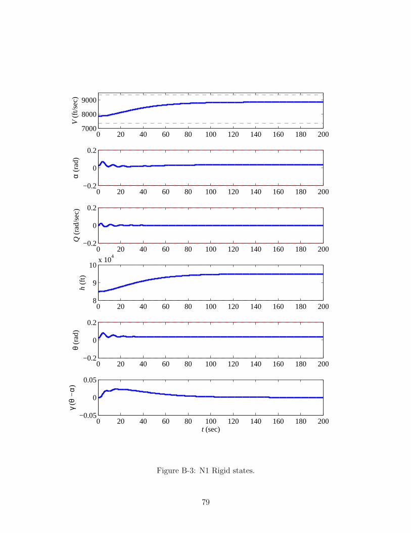
0 20 40 60 80 100 120 140 160 180 2007000
8000
9000
V (f
t/sec
)
0 20 40 60 80 100 120 140 160 180 200−0.2
0
0.2
α (r
ad)
0 20 40 60 80 100 120 140 160 180 200−0.2
0
0.2
Q (r
ad/s
ec)
0 20 40 60 80 100 120 140 160 180 2008
9
10x 10
4
h (f
t)
0 20 40 60 80 100 120 140 160 180 200−0.2
0
0.2
θ (r
ad)
0 20 40 60 80 100 120 140 160 180 200−0.05
0
0.05
γ (θ
−α)
t (sec)
Figure B-3: N1 Rigid states.
79

0 20 40 60 80 100 120 140 160 180 200−5
0
5LF
t (sec)
Figure B-4: N1 Loading Factor.
0 20 40 60 80 100 120 140 160 180 200−1
−0.5
0
0.5
1
θ
t (sec)
Figure B-5: N1 Adaptive parameters.
80
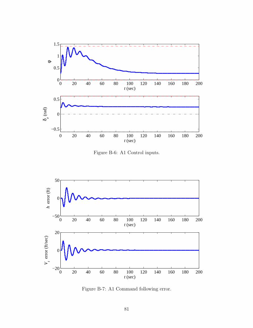
0 20 40 60 80 100 120 140 160 180 2000
0.5
1
1.5φ
t (sec)
0 20 40 60 80 100 120 140 160 180 200
−0.5
0
0.5
δ e (ra
d)
t (sec)
Figure B-6: A1 Control inputs.
0 20 40 60 80 100 120 140 160 180 200−20
0
20
Vt e
rror
(ft/
sec)
t (sec)
0 20 40 60 80 100 120 140 160 180 200−50
0
50
h e
rror
(ft)
t (sec)
Figure B-7: A1 Command following error.
81
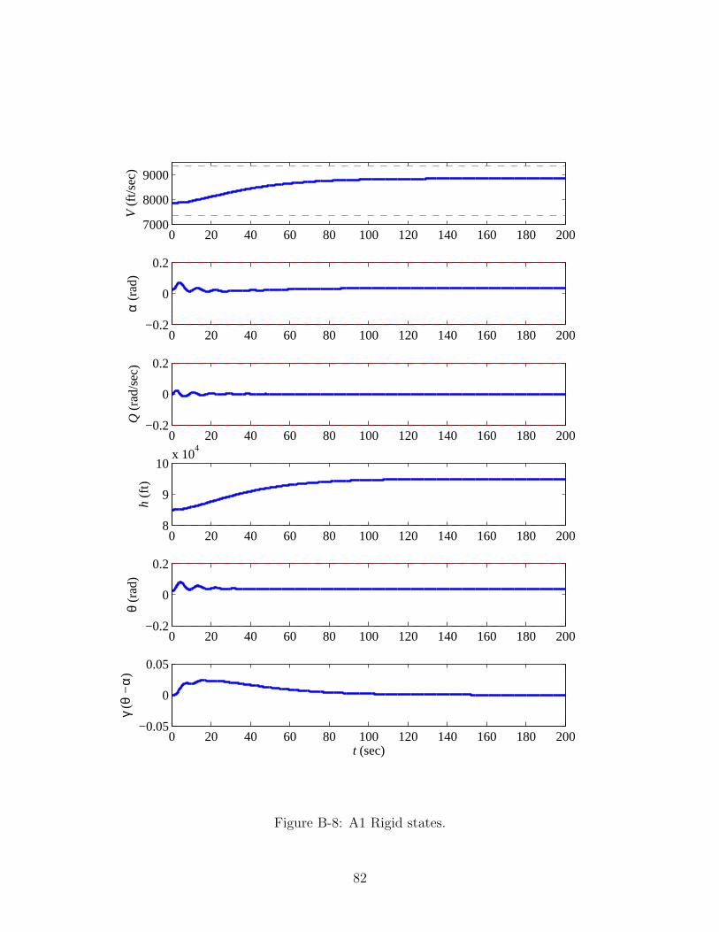
0 20 40 60 80 100 120 140 160 180 2007000
8000
9000
V (f
t/sec
)
0 20 40 60 80 100 120 140 160 180 200−0.2
0
0.2
α (r
ad)
0 20 40 60 80 100 120 140 160 180 200−0.2
0
0.2
Q (r
ad/s
ec)
0 20 40 60 80 100 120 140 160 180 2008
9
10x 10
4
h (f
t)
0 20 40 60 80 100 120 140 160 180 200−0.2
0
0.2
θ (r
ad)
0 20 40 60 80 100 120 140 160 180 200−0.05
0
0.05
γ (θ
−α)
t (sec)
Figure B-8: A1 Rigid states.
82
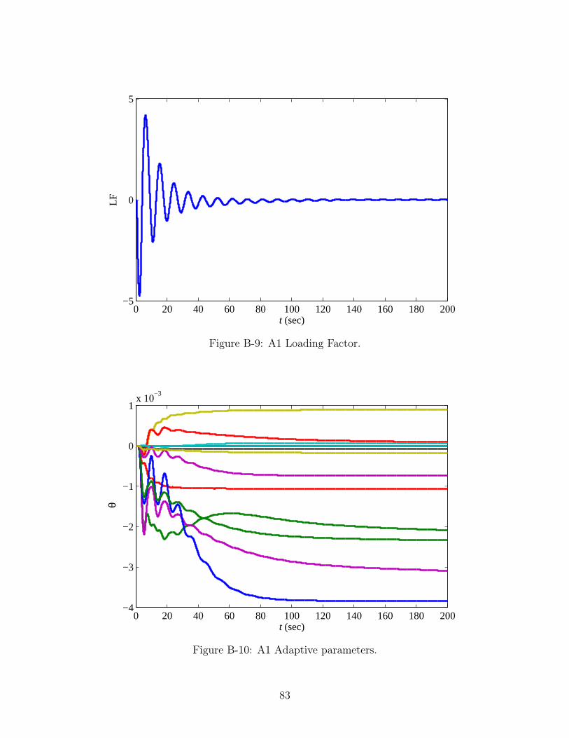
0 20 40 60 80 100 120 140 160 180 200−5
0
5LF
t (sec)
Figure B-9: A1 Loading Factor.
0 20 40 60 80 100 120 140 160 180 200−4
−3
−2
−1
0
1x 10
−3
θ
t (sec)
Figure B-10: A1 Adaptive parameters.
83
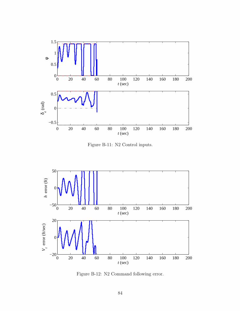
0 20 40 60 80 100 120 140 160 180 2000
0.5
1
1.5φ
t (sec)
0 20 40 60 80 100 120 140 160 180 200
−0.5
0
0.5
δ e (ra
d)
t (sec)
Figure B-11: N2 Control inputs.
0 20 40 60 80 100 120 140 160 180 200−20
0
20
Vt e
rror
(ft/
sec)
t (sec)
0 20 40 60 80 100 120 140 160 180 200−50
0
50
h e
rror
(ft)
t (sec)
Figure B-12: N2 Command following error.
84
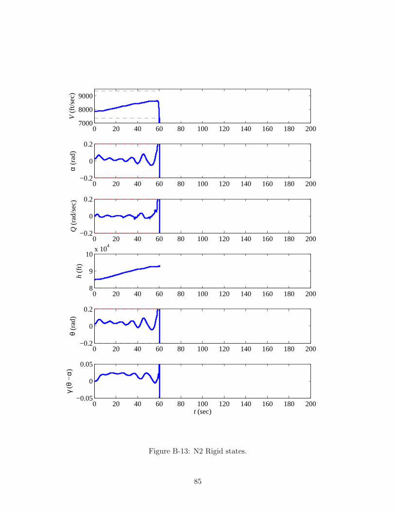
0 20 40 60 80 100 120 140 160 180 2007000
8000
9000
V (f
t/sec
)
0 20 40 60 80 100 120 140 160 180 200−0.2
0
0.2
α (r
ad)
0 20 40 60 80 100 120 140 160 180 200−0.2
0
0.2
Q (r
ad/s
ec)
0 20 40 60 80 100 120 140 160 180 2008
9
10x 10
4
h (f
t)
0 20 40 60 80 100 120 140 160 180 200−0.2
0
0.2
θ (r
ad)
0 20 40 60 80 100 120 140 160 180 200−0.05
0
0.05
γ (θ
−α)
t (sec)
Figure B-13: N2 Rigid states.
85

0 10 20 30 40 50 60 70−6000
−4000
−2000
0
2000
4000
6000
8000LF
t (sec)
Figure B-14: N2 Loading Factor.
0 10 20 30 40 50 60 70−1
−0.5
0
0.5
1
θ
t (sec)
Figure B-15: N2 Adaptive parameters.
86
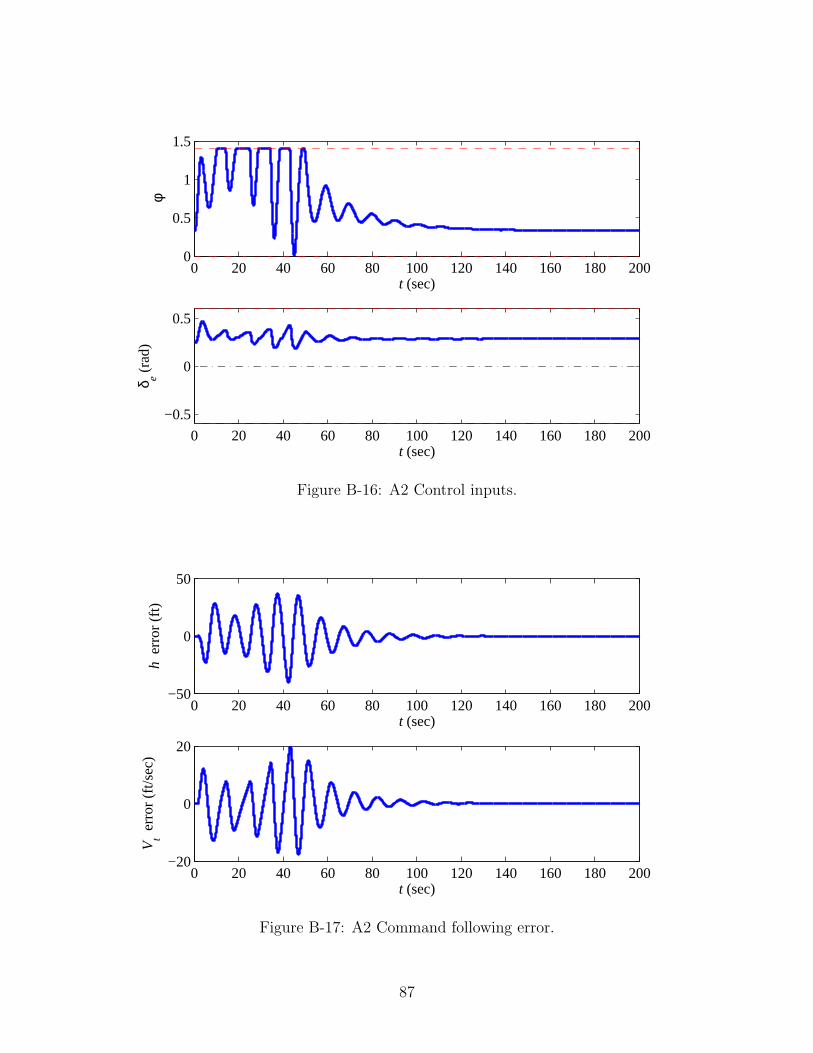
0 20 40 60 80 100 120 140 160 180 2000
0.5
1
1.5φ
t (sec)
0 20 40 60 80 100 120 140 160 180 200
−0.5
0
0.5
δ e (ra
d)
t (sec)
Figure B-16: A2 Control inputs.
0 20 40 60 80 100 120 140 160 180 200−20
0
20
Vt e
rror
(ft/
sec)
t (sec)
0 20 40 60 80 100 120 140 160 180 200−50
0
50
h e
rror
(ft)
t (sec)
Figure B-17: A2 Command following error.
87
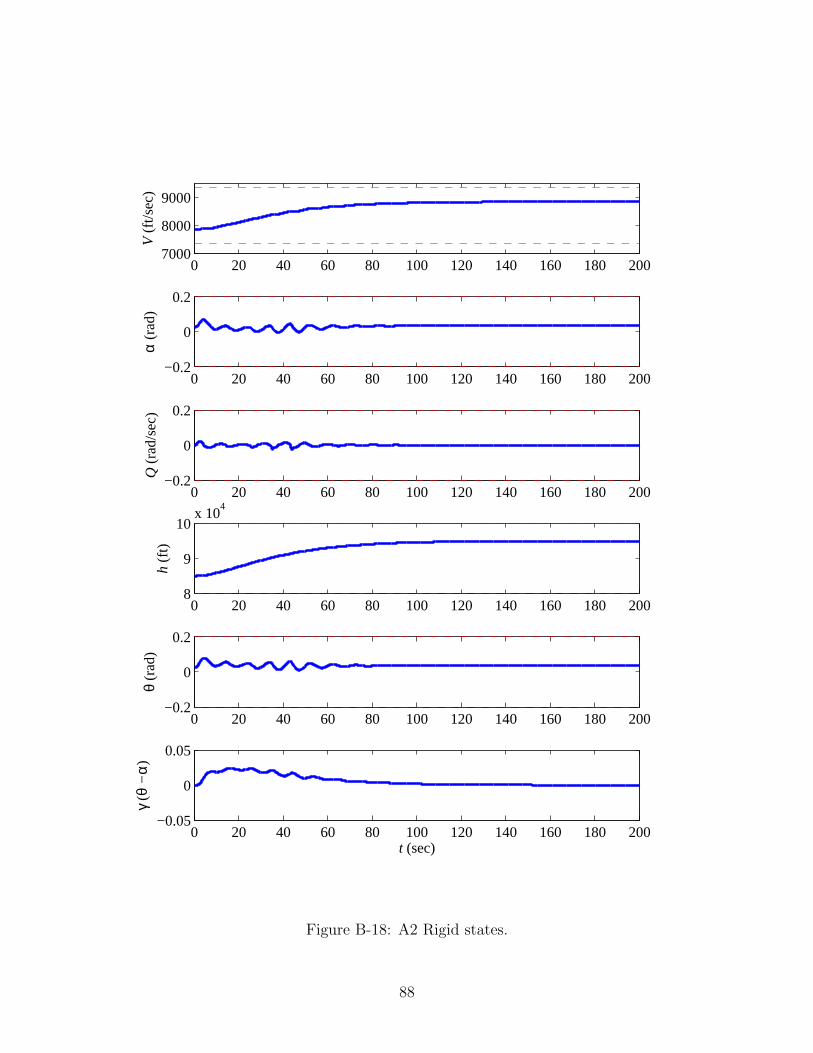
0 20 40 60 80 100 120 140 160 180 2007000
8000
9000
V (f
t/sec
)
0 20 40 60 80 100 120 140 160 180 200−0.2
0
0.2
α (r
ad)
0 20 40 60 80 100 120 140 160 180 200−0.2
0
0.2
Q (r
ad/s
ec)
0 20 40 60 80 100 120 140 160 180 2008
9
10x 10
4
h (f
t)
0 20 40 60 80 100 120 140 160 180 200−0.2
0
0.2
θ (r
ad)
0 20 40 60 80 100 120 140 160 180 200−0.05
0
0.05
γ (θ
−α)
t (sec)
Figure B-18: A2 Rigid states.
88
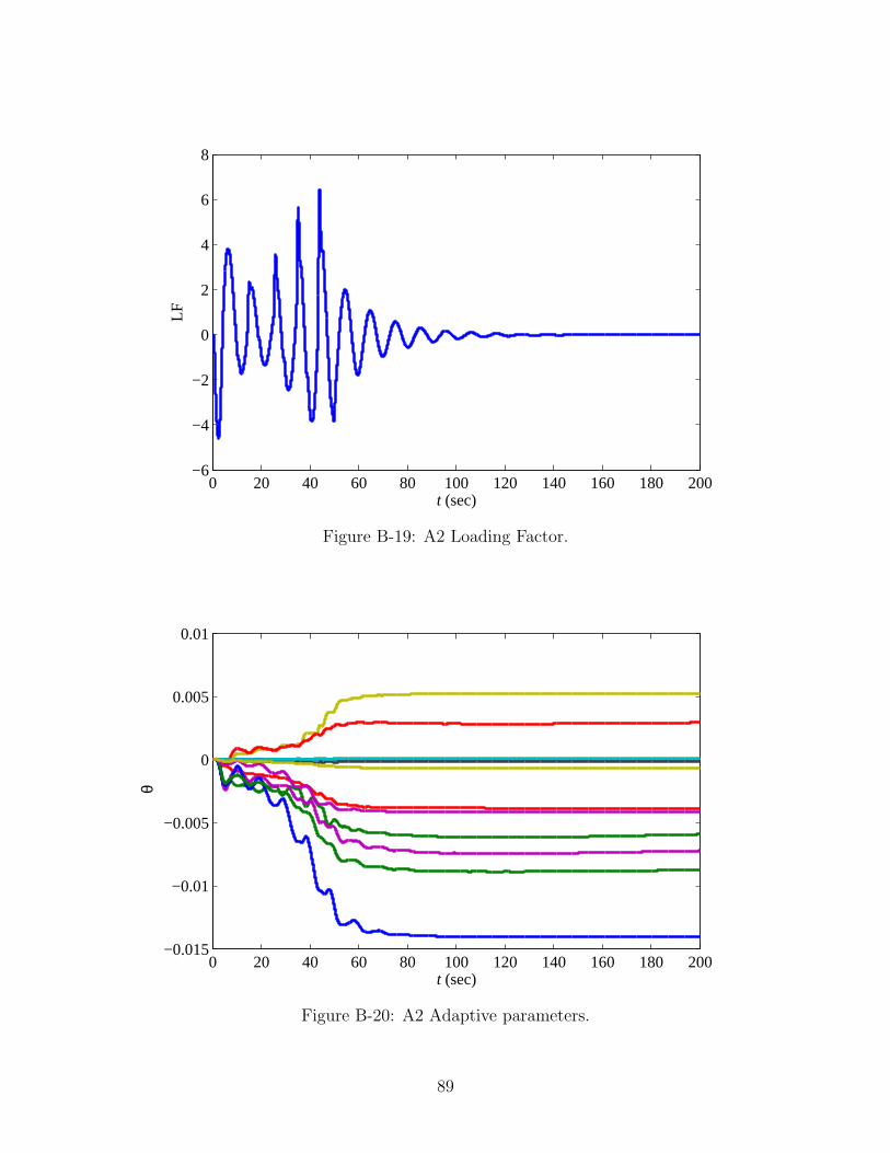
0 20 40 60 80 100 120 140 160 180 200−6
−4
−2
0
2
4
6
8LF
t (sec)
Figure B-19: A2 Loading Factor.
0 20 40 60 80 100 120 140 160 180 200−0.015
−0.01
−0.005
0
0.005
0.01
θ
t (sec)
Figure B-20: A2 Adaptive parameters.
89

0 20 40 60 80 100 120 140 160 180 2000
0.5
1
1.5φ
t (sec)
0 20 40 60 80 100 120 140 160 180 200
−0.5
0
0.5
δ e (ra
d)
t (sec)
Figure B-21: N3 Control inputs.
0 20 40 60 80 100 120 140 160 180 200−20
0
20
Vt e
rror
(ft/
sec)
t (sec)
0 20 40 60 80 100 120 140 160 180 200−50
0
50
h e
rror
(ft)
t (sec)
Figure B-22: N3 Command following error.
90

0 20 40 60 80 100 120 140 160 180 2007000
8000
9000
V (f
t/sec
)
0 20 40 60 80 100 120 140 160 180 200−0.2
0
0.2
α (r
ad)
0 20 40 60 80 100 120 140 160 180 200−0.2
0
0.2
Q (r
ad/s
ec)
0 20 40 60 80 100 120 140 160 180 2008
9
10x 10
4
h (f
t)
0 20 40 60 80 100 120 140 160 180 200−0.2
0
0.2
θ (r
ad)
0 20 40 60 80 100 120 140 160 180 200−0.05
0
0.05
γ (θ
−α)
t (sec)
Figure B-23: N3 Rigid states.
91
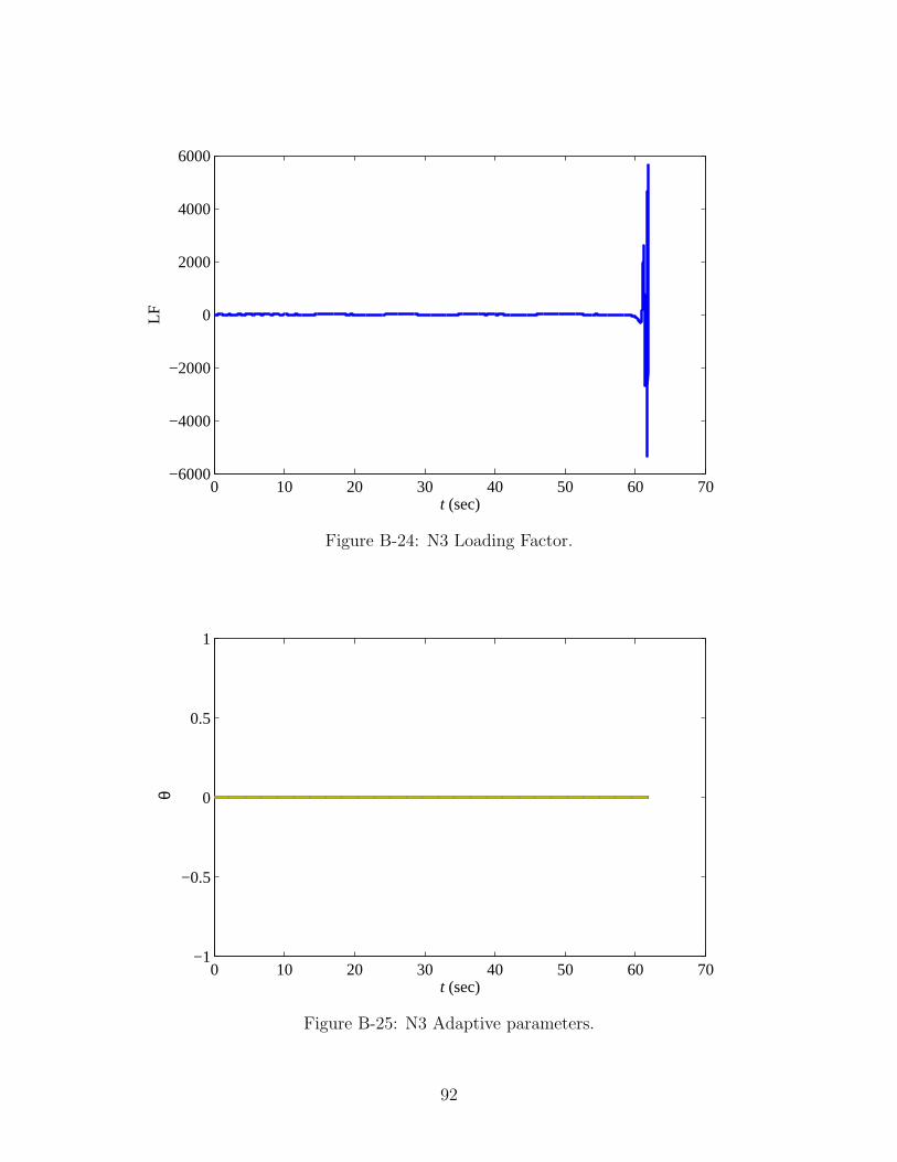
0 10 20 30 40 50 60 70−6000
−4000
−2000
0
2000
4000
6000LF
t (sec)
Figure B-24: N3 Loading Factor.
0 10 20 30 40 50 60 70−1
−0.5
0
0.5
1
θ
t (sec)
Figure B-25: N3 Adaptive parameters.
92
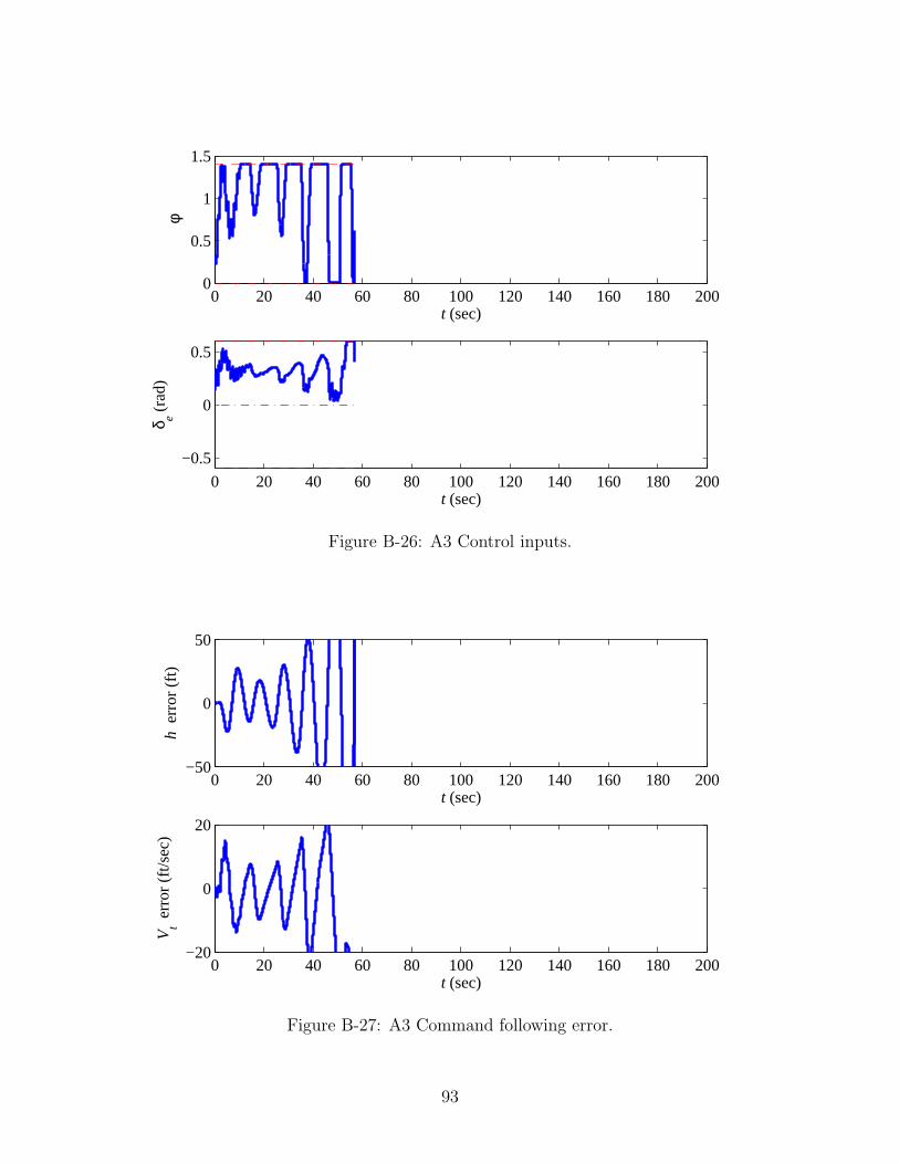
0 20 40 60 80 100 120 140 160 180 2000
0.5
1
1.5φ
t (sec)
0 20 40 60 80 100 120 140 160 180 200
−0.5
0
0.5
δ e (ra
d)
t (sec)
Figure B-26: A3 Control inputs.
0 20 40 60 80 100 120 140 160 180 200−20
0
20
Vt e
rror
(ft/
sec)
t (sec)
0 20 40 60 80 100 120 140 160 180 200−50
0
50
h e
rror
(ft)
t (sec)
Figure B-27: A3 Command following error.
93
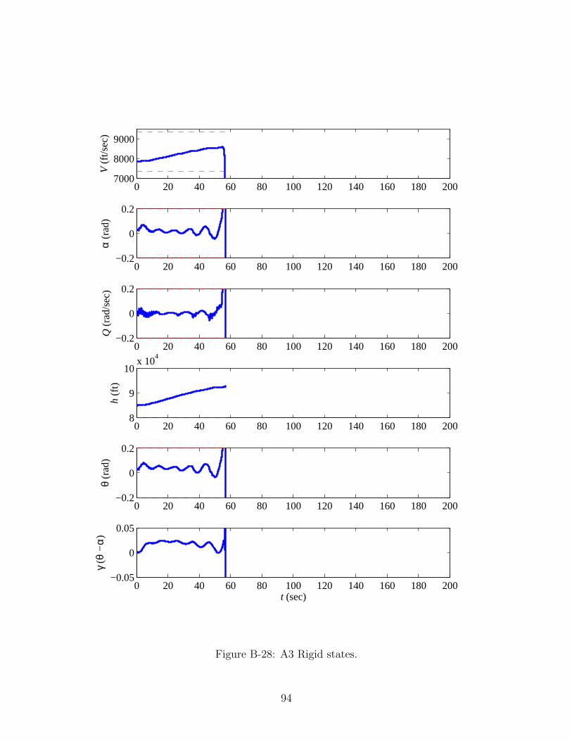
0 20 40 60 80 100 120 140 160 180 2007000
8000
9000
V (f
t/sec
)
0 20 40 60 80 100 120 140 160 180 200−0.2
0
0.2
α (r
ad)
0 20 40 60 80 100 120 140 160 180 200−0.2
0
0.2
Q (r
ad/s
ec)
0 20 40 60 80 100 120 140 160 180 2008
9
10x 10
4
h (f
t)
0 20 40 60 80 100 120 140 160 180 200−0.2
0
0.2
θ (r
ad)
0 20 40 60 80 100 120 140 160 180 200−0.05
0
0.05
γ (θ
−α)
t (sec)
Figure B-28: A3 Rigid states.
94
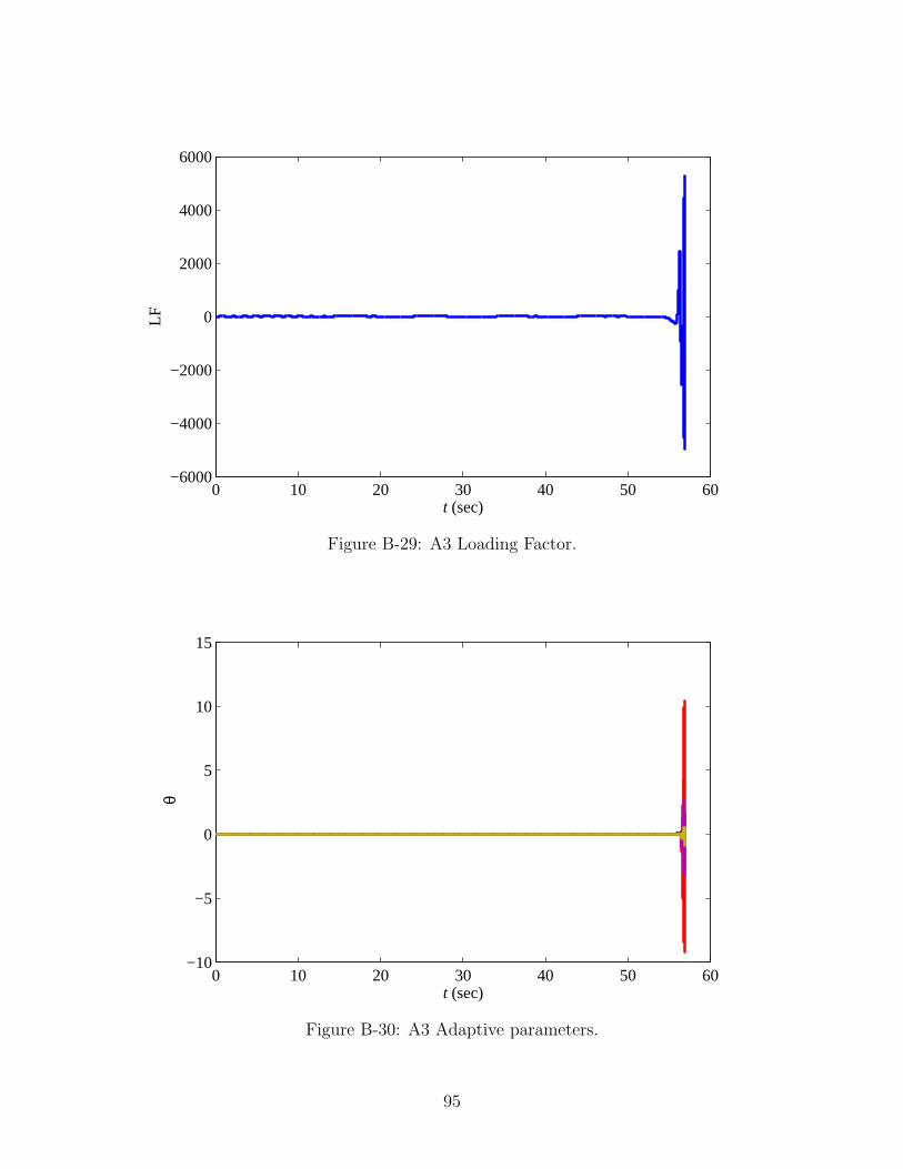
0 10 20 30 40 50 60−6000
−4000
−2000
0
2000
4000
6000LF
t (sec)
Figure B-29: A3 Loading Factor.
0 10 20 30 40 50 60−10
−5
0
5
10
15
θ
t (sec)
Figure B-30: A3 Adaptive parameters.
95
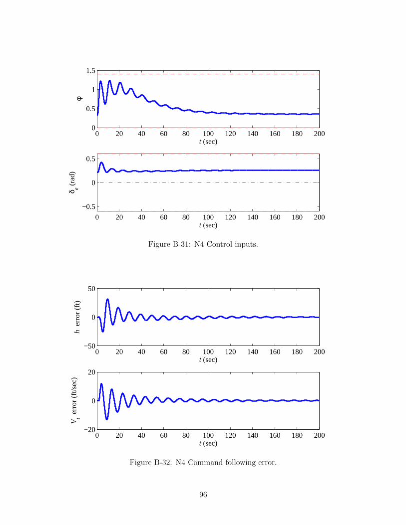
0 20 40 60 80 100 120 140 160 180 2000
0.5
1
1.5φ
t (sec)
0 20 40 60 80 100 120 140 160 180 200
−0.5
0
0.5
δ e (ra
d)
t (sec)
Figure B-31: N4 Control inputs.
0 20 40 60 80 100 120 140 160 180 200−20
0
20
Vt e
rror
(ft/
sec)
t (sec)
0 20 40 60 80 100 120 140 160 180 200−50
0
50
h e
rror
(ft)
t (sec)
Figure B-32: N4 Command following error.
96
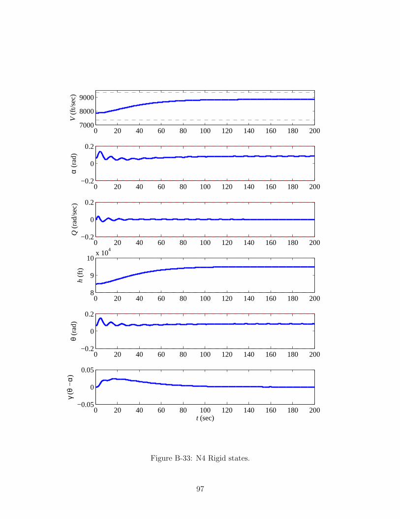
0 20 40 60 80 100 120 140 160 180 2007000
8000
9000
V (f
t/sec
)
0 20 40 60 80 100 120 140 160 180 200−0.2
0
0.2
α (r
ad)
0 20 40 60 80 100 120 140 160 180 200−0.2
0
0.2
Q (r
ad/s
ec)
0 20 40 60 80 100 120 140 160 180 2008
9
10x 10
4
h (f
t)
0 20 40 60 80 100 120 140 160 180 200−0.2
0
0.2
θ (r
ad)
0 20 40 60 80 100 120 140 160 180 200−0.05
0
0.05
γ (θ
−α)
t (sec)
Figure B-33: N4 Rigid states.
97
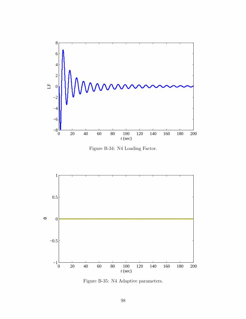
0 20 40 60 80 100 120 140 160 180 200−8
−6
−4
−2
0
2
4
6
8LF
t (sec)
Figure B-34: N4 Loading Factor.
0 20 40 60 80 100 120 140 160 180 200−1
−0.5
0
0.5
1
θ
t (sec)
Figure B-35: N4 Adaptive parameters.
98
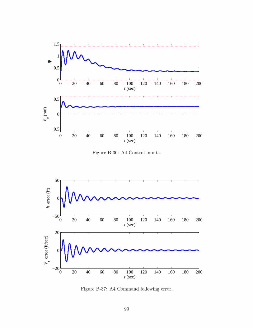
0 20 40 60 80 100 120 140 160 180 2000
0.5
1
1.5φ
t (sec)
0 20 40 60 80 100 120 140 160 180 200
−0.5
0
0.5
δ e (ra
d)
t (sec)
Figure B-36: A4 Control inputs.
0 20 40 60 80 100 120 140 160 180 200−20
0
20
Vt e
rror
(ft/
sec)
t (sec)
0 20 40 60 80 100 120 140 160 180 200−50
0
50
h e
rror
(ft)
t (sec)
Figure B-37: A4 Command following error.
99
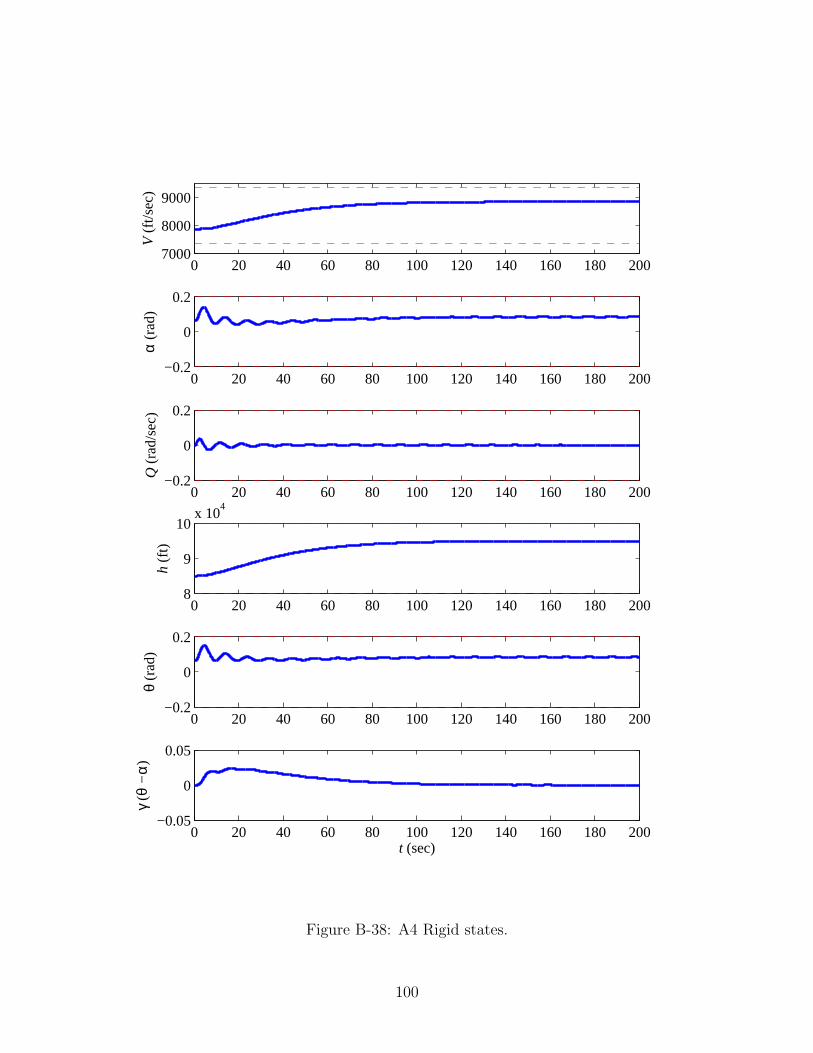
0 20 40 60 80 100 120 140 160 180 2007000
8000
9000
V (f
t/sec
)
0 20 40 60 80 100 120 140 160 180 200−0.2
0
0.2
α (r
ad)
0 20 40 60 80 100 120 140 160 180 200−0.2
0
0.2
Q (r
ad/s
ec)
0 20 40 60 80 100 120 140 160 180 2008
9
10x 10
4
h (f
t)
0 20 40 60 80 100 120 140 160 180 200−0.2
0
0.2
θ (r
ad)
0 20 40 60 80 100 120 140 160 180 200−0.05
0
0.05
γ (θ
−α)
t (sec)
Figure B-38: A4 Rigid states.
100
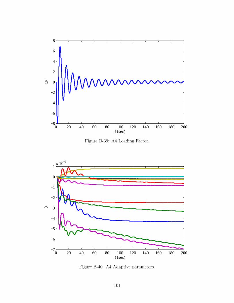
0 20 40 60 80 100 120 140 160 180 200−8
−6
−4
−2
0
2
4
6
8LF
t (sec)
Figure B-39: A4 Loading Factor.
0 20 40 60 80 100 120 140 160 180 200−7
−6
−5
−4
−3
−2
−1
0
1x 10
−3
θ
t (sec)
Figure B-40: A4 Adaptive parameters.
101

102
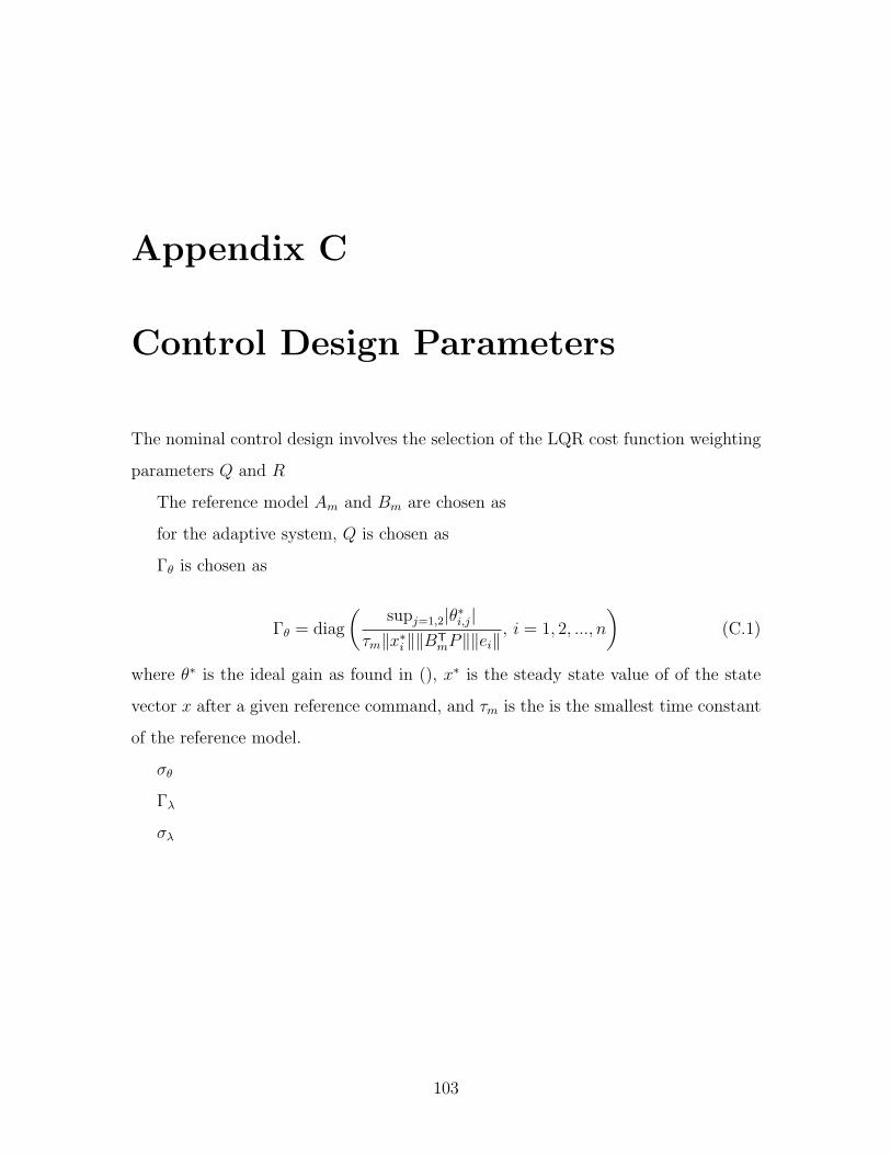
Appendix C
Control Design Parameters
The nominal control design involves the selection of the LQR cost function weighting
parameters Q and R
The reference model Am and Bm are chosen as
for the adaptive system, Q is chosen as
Γθ is chosen as
Γθ = diag
(supj=1,2|θ∗i,j|
τm‖x∗i ‖‖BTmP‖‖ei‖
, i = 1, 2, ..., n
)(C.1)
where θ∗ is the ideal gain as found in (), x∗ is the steady state value of of the state
vector x after a given reference command, and τm is the is the smallest time constant
of the reference model.
σθ
Γλ
σλ
103

104
Bibliography
[1] R. J. Admas and et al. Robust Multivariable Flight Control. Springer-Verlag,1994.
[2] John D. Anderson. Modern Compressible Flow: with Hystorical Perspective.McGraw-Hill Science, 2002.
[3] Anon. Equations, tables, and charts for compressible flow. Technical ReportNACA–1135, Ames Aeronautical Laboratory, National Advisory Committee forAeronautics, Moffett Field, CA, 1953.
[4] Anon. Handbook of Aviation Fuel Properties. Coordinating Research Council,Atlanta, GA, 1983.
[5] Anon. Dryden flight research center nasa graphics x–43a/hyper–x, 2004. http:
//www.dfrc.nasa.gov/Gallery/Graphics/X-43A/index.html.
[6] Anon. Dryden flight research center nasa images x–43a/hyper–x, 2004. http:
//www.dfrc.nasa.gov/Gallery/Photo/X-43A/Large/index.html.
[7] Michael A. Bolender and David B. Doman. Nonlinear longitudinal dynamicalmodel of an air-breathing hypersonic vehicle. Journal Spacecraft and Rockets,44(2), March-April 2007.
[8] Michael A. Bolender and Davod B. Doman. Flight path angle dynamics ofair-breathing hypersonic vehicles. In AIAA Guidance, Navigation, and ControlConference and Exhibit, 21-24 August 2006. Keystone,Colorado.
[9] Michael A. Bolender, Michael W. Oppenheimer, and David B. Doman. Effects ofunsteady and viscous aerodynamics on the dynamics of a flexible air-breathinghypersonic vehicle. In AIAA GAFMC, August 2007. Hilton Head, South Car-olina.
[10] Frank R. Chavez and David K. Schmidt. Analytical aeropropulsive/aeroelastichypresonic-vehicle model with dynamic analysis. Journal of Guidance, Control,and Dynamics, 17(6), Nov-Dec 1994.
[11] Andrew Clark, Chivey Wu, Maj Mirmirani, Sangbum Choi, and MathewKuipers. Development of an airframe-propulsion integrated generic hypersonic
105
vehicle model. In AIAA Aerospace Sciences Meetings and Exhibit, January 2006.Reno, Nevada.
[12] R. D. Colgren. Nonlinear h-inf control of a missle’s roll axis. ACC, 1994. Balti-more, MD.
[13] R. D. Colgren, D. Enns, and et al. Structured singular value synthesis appliedto the f–117a. In IFAC World Congress, 1996. San Francisco, CA.
[14] L. G. Crespo, D. P. Giesy, and S. P. Kenny. Robust analysis and robust designof uncertain systems. AIAA Journal, 46(2), 2008.
[15] L.G. Crespo. Sampling-based techniques for the estimation of probabilistic sen-sitivities. In AIAA NDA, 2008.
[16] L.G. Crespo. A verification-driven approach to control tuning. In AIAA Guid-ance, Navigation, and Control Conference and Exhibit, 2008.
[17] Z. Dydek, H. Jain, J. Jang, A. Annaswamy, and E. Lavretsky. Theoreticallyverifiable stability margins for an adaptive controller. In AIAA Guidance,Navigation, and Control Conference and Exhibit, 21-24 August 2006. Key-stone,Colorado.
[18] Zachary T. Dydek. Guaranteed margins and performance for an adaptive flightcontrol system and application on the x-15 research airplane. Master’s thesis,Massachusetts Institute of Technology.
[19] L. Fiorentini, A. Serrani, Michael A. Bolender, and David B. Doman. Non-linear robust/adaptive controller design for an air-breathing hypersonic vehiclemodel. In AIAA Atmospheric Flight Mechanics Conference and Exhibit, Aug.20-23 2007. Hilton Head, South Carolina.
[20] L. Fiorentini, A. Serrani, Michael A. Bolender, and David B. Doman. Nonlinearcontrol of a hypersonic vehicle with structural flexibility. In IEEE Conferenceon Decision and Control, 2008. Submitted.
[21] Travis E. Gibson and Anuradha M. Annaswamy. Adaptive control of hyper-sonic vehicles in the presence of thrust and actuator uncertainties. In AIAAGuidance, Navigation, and Control Conference and Exhibit, 18-21 August 2008.Honolulu,Hawaii.
[22] K.P. Groves, A. Serrani, S. Yurkovich, M. Bolender, and D. Doman. Anti-windup control for an air-breathing hypersonic vehicle model. In AIAA GuidanceNavigation and Controls Conference and Exhibit, Aug. 21-24 2006. Keystone,Colorado.
[23] K.P. Groves, D.O. Sigthorsson, A. Serrani, S. Yurkovich, M. Bolender, and D. Do-man. Reference command tracking for a linearized model of an air-breathinghypersonic vehicle. In AIAA Guidance, Navigation, and Control Conference andExhibit, 15-18 August 2005. San Francisco,California.
106
[24] W. Heiser and D. Pratt. AIAA, Washington, D.C., 1994, pp. 109–143.
[25] R. A. Hyde. H–inf Aerospace Control Design: A VSTOL Flight Application.Springer-Verlag, 1995.
[26] H. Ikawa. Rapid methodology for design and performance prediction of integratedsupersonic combustion ramjet engine. 17(3):437, 1991.
[27] J. Jang, A. M. Annaswamy, and E. Lavretsky. Adaptive flight control in thepresence of multiple actuator anomalies. In Proceedings of the 2007 AmericanControl Conference, pages 3300–3305, New York, NY,20-23 August 2007.
[28] J. Jang, A. M. Annaswamy, and E. Lavretsky. Adaptive flight control in thepresence of multi-input magnitude saturation. In (to appear) IEEE Conferenceon Decision and Control, Cancun, Mexico, Dec. 2008.
[29] Dennis R. Jenkins. Hypersonic before the shuttle: A concise history of ther x-15research plane. Monographs In Aerospace History 18, National Aeronautics andSpace Administration, Washington, D.C., 2000.
[30] J.Levin, P. Ioannou, and M. Mirmirani. Adaptive mode suppression scheme foran aeroelastic airbreathing hypersonic cruise vehicle. In AIAA Guidance, Naviga-tion, and Control Conference and Exhibit, 18-21 August 2008. Honolulu,Hawaii.
[31] M. Kuipers, P. Ioannou, B.Fidan, and M. Mirmirani. Robust adaptive multiplemodel controller design for an airbreathing hypersonic vehicle model. In AIAAGuidance, Navigation, and Control Conference and Exhibit, 18-21 August 2008.Honolulu,Hawaii.
[32] M. Kuipers, M. Mirmirani, P. Ioannou, and Y. Huo. Adaptive control of anaeroelastic airbreathing hypersonic cruise vehicle. In AIAA Guidance, Naviga-tion, and Control Conference and Exhibit, 20-23 August 2007. Hilton Head,SouthCarolina.
[33] J. F. Magni, S. Bennani, and J. T. (eds.). Robust flight control: a design chal-lenge. Springer, 1997.
[34] C. I. Marrison and R. F. Stengel. Design of robust control systems for a hyper-sonic aircraft. AIAA GCD, 21:58–63, 1998.
[35] Laurie A. Marshall, Griffin P. Corpering, and Robert Sherrill. A chief engineer’sview of the nasa x–43a scrmajet flight test. In AIAA-2005-3332, 2005.
[36] NACA. Air Force - NACA Conference on XS–1 Flight Research, Muroc, CA,1948. NASA Historical Reference Collection.
[37] Richard D. Neumann. Defining the aerothermodynamic methodology. In Hyper-sonics:v. 1 : Defining the Hypersonic Environment, page 127. 1989.
107
[38] J.T. Parker, A. Serrani, S. Yurkovich, M. Bolender, and D. Doman. Approximatefeedback linearization of an air-breathing hypersonic vehicle. In AIAA GuidanceNavigation and Controls Conference and Exhibit, Aug. 21-24 2006. Keystone,Colorado.
[39] J.T. Parker, A. Serrani, S. Yurkovich, M. Bolender, and D. Doman. Control-oriented modeling of an air-breathing hypersonic vehicle. Journal of Guidance,Control, and Dynamics, 30(3), May-June 2007.
[40] D. Sigthorson, A. Serrani, S. Yurkovich, M. Bolender, and D. Doman. Trackingcontrol for an overactuated hypersonic air-breathing vehicle with steady stateconstraints. In AIAA Guidance Navigation and Controls Conference and Exhibit,Aug. 21-24 2006. Keystone, Colorado.
[41] D. 0. Sigthorson, P. Jankovsky, A. Serrani, S. Yurkovich, M. Bolender, andD. Doman. Robust linear output feedback control of an airbreathing hypersonicvehicle. Journal of Guidance, Control, and Dynamics, 31(4), July-August 2008.
[42] R. F. Stengel, J. R. Broussard, and P. W. Berry. Digital controllers for vtolaircraft. IEEE Aerospace and Electronic Systems, AES 14(1):54–63, 1978.
[43] Robert F. Stengel. Optimal Control and Estimation. Dover, New York, 1994.
[44] Robert F. Stengel. Flight Dynamics. Princeton University Press, Princeton andOxford, 2004.
[45] Wendell H. Stillwell. X–15 research results. Sp 60, National Aeronautics andSpace Administration, Washington, D.C., 1965.
[46] M. O. Thompson. At the edge of space: The x-15 flight program. SmithsonianInstitution Press, Washington DC, 1992.
[47] USAF. Air Force Supersonic Research Airplane XS–1 Report No. 1. NASAHistorical Reference Collection, 1947.
[48] Qian Wang and Robert F. Stengel. Robust nonlinear control of a hypersonicaircraft. Journal of Guidance, Control, and Dynamics, 23(4), Jul-Aug 2000.
[49] Qian Wang and Robert F. Stengel. Robust control of nonlinear systems withparametric uncertainty. Automatica, 38:1591–1599, 2002.
[50] R. J. Weber and J. S. Mackay. An analysis of ramjet engines using supersoniccombustion. Technical Report NACA TN–4386, Sept 1958.
[51] Haojian Xu, Maj D. Mirmirani, and Petros Ioannou. Adaptive sliding modecontrol design for a hypersonic flight vehicle. Journal of Guidance, Control, andDynamics, 27(5), Sept-Oct 2004.
108