Adaptive Control of S ace Robot System with an Attitude 8 ontrolled Base

Yangsheng Xu, Heung-Yeung Shum, Ju-Jang Lee, and Takeo Kanade

CMU-RI-TR-91-14

The Robotics Institute Carnegie Mellon University

Pittsburgh, Pennsylvania 15213

August 1991

01991 Cvnegie Mellon University

Contents

1 Introduction 1

2 Kinematics of Space Robot Syatem with An Attitude Controlled Base 2

3 Dynamics of Space Robot System with An Attitude Controlled Base 5

4 Adaptive Control Scheme 8

5 Adaptive Control in Inertia Space 12

6 Simulation Study 13

7 Conclusiona 17

References 24

i

.

List of Figures

1

2 3 4

5

6 7 8 9 10

11

Space robot system with au attitude controlled base . . . . . . . . . Block diagram of adaptive controller in joint space . . . . . . . . . . Block diagram of adaptive control scheme in inertia space . . . . . . Planar space robot system model . . . . . . . . . . . . . . . . . . . . Tracking errors and parameter estimations using joint space adap- tivecontrol . . . . . . . . . . . . . . . . . . . . . . . . . . . . . . . . 18 Comparison between adaptive control and dynamic control . . . . . . 19 Example of adaptive control for ked-baaed robot . . . . . . . . . . . 20 nlustration of combined dynamic parameter identification . . . . . . 21 Comparison between PD type and PID type adaptive control schemes . 22

adaptive controller . . . . . . . . . . . . . . . . . . . . . . . . . . . . 23

space adaptive controller . . . . . . . . . . . . . . . . . . . . . . . . . 23

2

11 13 14

Trajectories in joint space and in inertia space using inertia span

Tracking errors in joint space and in inertia space using inertia

ii

--

ABSTRACT

In this report, we discuss adaptive control of a space robot system with an

attitude controlled base on which the robot is attached. We at first derive the

system kinematic and dynamic equations based on Lagrangian dynamics and linear

momentum conservation law. Using the dynamic model developed, we discuss the

problem of linear parameterization in t m s of dynamic parameters, and have found

that in joint space the dynamics can be linearized by a set of combined dynamic

parameters, but in inertia space linear parameterization is impossible in general.

Then we propose an adaptive control scheme in joint space which has been shown

effective and feasible for the case where unknown or unmodeled dynamics must

be considered, such as in the tasks of transport an unknown payload, or catching

a moving object. The scheme avoids the use of joint acceleration measurement,

inversion of inertial matrix, high gain feedback, and considerable computation

cost, and at meantime, is also applicable for the fixed-base robot system by slight

modification. Since moat tasks are specified in inertia space, instead of joint space, we discuss the issues associated to adaptive control in inertia space and identify two

potential problems, unavailability of joint trajectory since mapping from inertia

space trajectory is dynamic dependent and subject to uncertainty, and nonlinear

Parameterization in inertia space. We approach the problem by making use of the propoaed joint space adaptive controller and updating joint trajectory by the

estimated dynamic parameters and given trajectory in inertia space. In the case

study of a planar system, the linear parameterization problem is investigated, the

design procedure of the controller is illustrated, and the validity and effectiveness

of the proposed control scheme is demonstrated.

1 Introduction

Considerable research efforts have been direeted to some primary functions of robots in space appli- cations, such as material transport 1171, simple manipulation (41, basic locomotion [14], inspection and maintenance of the space station and satellites [I, 41. The adaptive contml is critical for the robot system subject to dynamic uncertainty in these tasks.

For material transport and manipnlation tasks, space robots have to face uncertainty on the parameters describing the dynamic properties of the grasped load, such as moments of inertia or exact poaition of the mass center. In most caws, these parmeters are unknown and thus they can not be specified off-line, in in- dynamics for feedforward compensation or any model- based control scheme. In catching a moving object [15], the robot is expected to be capable of adaptation to the dynamies change at the moment of catching operation. On the other hand, most space robota are desiepeed to be light-weighted and thus low-powered, partially due to the fact zero gravity environment. Therefore, wit friction and damping in space robots are much more significant than those in industrial robots. These dec te are .either negligible nor easy to model. Adaptive control may provide a feasjble solution to those system dynamica uncertainties. Adaptive control is a h able to accommodate various nnmodeled disturbances, such as base diaturbance, microgravity effect, eenaor and actuator noise due to extrema of temperature and glare, or impact effect during docking or rendezvous process.

Most of existing adaptive control algorithms have the following shortcomings which cause their applications in space robots unrealistic, the u ~ e of joint acceleration measurement, the need of inversion of inertia matrix, high gain feedback and considerable computational cost. The first two must be avoided even for fixed-base induetrid robots, because of lack of joint acceleration sensor and the complexity of inversion of inertia matrix. Slotine and Li 1111 have tackled these problems succeaafuly. A high gain feedback is extremely h a r d for a space robot which is usually light-weighted and l o w - p o d . considerable computation also need13 to be avoided for allowable package of self-contained space robots.

This report focuses on the robot system where the base attitude is controlled by either thrust jets, or reaction wheels. The reaction wheels are arranged in orthogonal directions, and the number of reaction wheels can be three or two depending on Merent trsks, and a standard reaction wheel configuration can be fonnd in [SI. When the attitude of the base is controlled, the orientation and position of both robot and base are no longer free, and the dynamic interaction between the base and robot results in the dynamic dependent kinematics, i.e., the kinematics is in relation to the mass property of the base and robot. Control is not only applied to robot joint angles, but also three orientations of the base.

In this report, based on hear momentum conservation law and Lagrangian dynamics, we at first formulate kinematics and dynamics equations of the space robot system with an attitude controlled base, in a systematic way. Based on the dynamic model developed, we study the linear parameterization problem, i.e., dynamics can he liaeorly e x p r d in terms of dynamic parameters, such as mass and inertia. We have found that for the space robot system with an attitude control base, the linear parameterization is valid in pit space, while is not valid in inertia space which can be viewed as Cartesian space for ea r th -bad robots.

Ueing the dynamic model, we propose an adaptive control scheme in joint apace. The scheme does not need to measure accelerations in j t i i t space, and a high feedback gain is not required. The proposed method is dective and feasible for EF robot applications when dynamic parameters are unknown or unmodeled dynamies effect must be considered. Since in most appEcations, the tasks are specified in inertia space normally, instead of joint space, we &ws the issues in relation

1

T

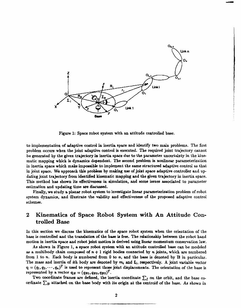
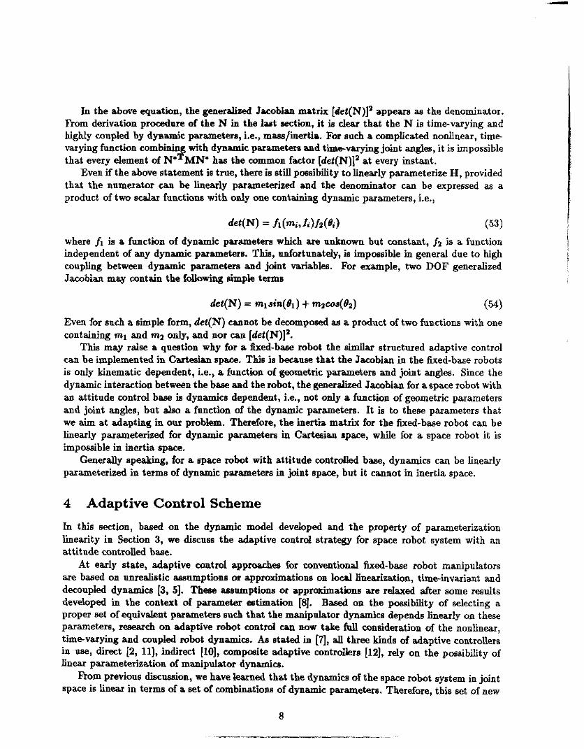
Figure 1: Space robot system with an attitude controlled base.

to implementation of adaptive control in inertia space and identify two main problems. The first problem occurs when the joint adaptive control is executed. The required joint trajectory cannot be generated by the given trajectory in inertia space due to the parameter uncertainty in the kine- matic mapping which is dynamics dependent. The seeond problem is nonlinear parameterization in inertia space which make impossible to implement the same structured adaptive control as that in joint space. We approaeh this problem by masing une of joint SpaCe adaptive wntroller and up- dating joint trajectory from identified kinematic mapping and the given trajectory in inertia space. This method has shown its dectiveness in simulation, and some issues associated to parameter estimation and updating time are discussed.

Finally, we study a planar robot system to investigate linear parameterization problem of robot system dynamics, and illustrate the validity and effectiveness of the proposed adaptive control S C h e m e S .

2 Kinematics of Space Robot System with An Attitude Con- trolled Base

In this Bection we discuss the kinematics of the space robot system when the orientation of the base is controlled and the translation of the base ia free. The relationship between the robot hand motion in inertia space and robot pint motion is derived using linear momentum conservation law.

As shown in Figure 1, a space robot system with an attitude controUed base can be modeled as a multibody chain composed of R + 1 rigid bodies connected by R Hits, which are numbered from 1 to n. Each body in numbered from 0 to n, and the base is denoted by B in particular. The ma88 and inertia of ith body are denoted by mi and Ii, respectively. A joint variable vector q = (ql,a,-**,qn)T is used to represent thosepint displacements. The orientation of the base is represented by a vector qB = ( q ~ , , 4 ~ ~ , 4 ~ 3 ) ~ .

Two coordinate frames are d e h d , the inertia coordinate Cr on the orbit, and the base co- ordinate CB attached on the baae body with it8 origin at the centroid of the base. As shown in

2

Figure 1, let & and r; be the position vectors pointing the centroid of ith body with reference to and CB respectively, then

&=ri+RB (1) where Rg is the position vector pointing the centroid of the bas-? with reference to El. Let V; and S I ; be hear and angular velocitia of ith body with respect to El, v; and wi with respect to CB. Then we have

where Vg and RB are hem and angular velocities of the centroid of the base with respect to &, and operator 'x' represents outer prodact of R3 vector. The velocities vi and wi in base coordinates can be represented by

V; = Jfi(q)il (3)

Ui = JAi(q)il (4)

where Jfi(q) and Jli(q) are the submatrim of Jacobian of the ith body representing linear part and angular part respectively. The centroid of the total system can be determined by

n m, = C m i

i=o

I, = C I i i d

( 5 )

The linear momentum can be determined by

where Hv = m,U3

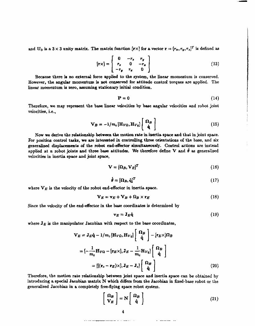
and U, is a 3 x 3 unity matrix. The matrix function (rx] for a vector r = [r=, r,,,tJT is defined as

[ r x l = [ -: <=] (13) -Tu T r

Because there is no external force applied to the system, the linear momentum is conserved. Howvex, the mguk momentum is aot w d for attitude control torques are applied. The hear momentum is zero, assuming stationary initial condition.

P=O (14) Therefore, we may represent the base linear velocities by base angular velocities and robot joint velocities, Le.,

Now we derive the relationship between the. motion rate in inertia pace and that in joint space. For position control tasks, we are interested in controlling three orientations of the base, and six generalized displacemedo of the robet end-dectur sheltawously. Control actions are instead applied at n robot joint8 and three bane attitudes. We therefore define V and 8 as generalized velocities in inertia space and joint space,

v = [ Q B , V E I T (16)

B = [QB,;I]T

where V E is the veloeity of the robot end-effector in inertia space.

V E = VE + v B + n B x r E (18)

V E = J E ~ (19)

Since the velocity of the end-dector in the base coordinates is determined by

where JE is the manipulator Jacobian with respect to the base coordinates,

Therefore, the motion rate relationship between joint space and inertia space can be obtained by introducing a special Jacobian matrix N which diiFem from the Jacobian in ked-base robot or the generalized Jacobian in a completely free-flying space robot system.

4

where

and Os is a 3 x 3 m m a t r i x .

3 Dynamics of Space Robot System with An Attitude Con- trolled Base

In this seetion we discuss dynamics of the sp"e robot system with an attitude controlled base. After formulating total kinetic energy of the aystem we derive the dynamics equation of the system. Then we investigate the property of linear parameterization of the system dynamics which is critical for developing the adaptive control algorithms in the following seetion.

The total system kinetic energy is represented by

= 1/2dTM(b')d (25) where M ia the inertia matrix of the system, H, is the robot inertia matrix in base coordinate, i.e., fixed base inertia matrix. and

8 = 198, dT (26)

5

I-_- _ _ _ -

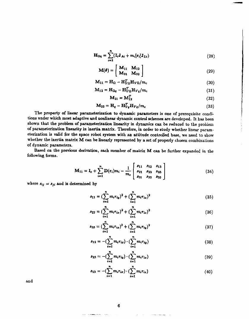
Mi1 = Hn - H$&vn/mc

Miz = Hnq - H?nHvq/mc

Maa = Hp - H$$b*/m,

(30)

(31)

(33) Mm = MTa (32)

The property of linear Parameterization to dynamic parameters i B one of prerequisite condi- tions under which most adaptive and nonlinear dynamic eontrd schemes are developed. It h a been shown that the problem of parameterization linearity in dynamics can be reduced to the problem of parameterization linearity in inertia matrix. Therefore, in order to study whether h e a r paran- eterization is valid for the apace robot syetem with an attitude controlled base, we need to show whether the inertia matrix M can be linearly represented by a set of properly chosen combinations of dynamic parameters.

Based on the previous derivation, each member of matrix M UUL be further expanded in the following forms.

where s;j = 8,; and is determined by

i=l i=l

and

.-

I

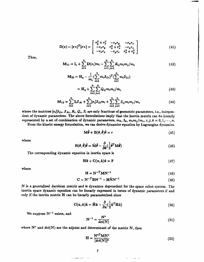
Thus.

n n n n

Mi1 = C I i J A i + c[ri]J~.imi + ~ ~ S i j m i m j / m , (44) i=l i r l i=l j=1

where the matrices [riJJfi, JA;, Ri, Q;, Si are only functions of geometric parameters, i.e., indepen- dent of dynamic parameters. The above formulations imply that the inertia matrix can be linearly represented by a set of combhation of dynamic parameters, mk, 4, mirnjlm,, i,j, k = 0,1, * . . , n.

From the kinetic energy formulation, we can derive dynamics equation by Lagrangian dynamics.

M8 + B(B,d)i = r (45)

where a 1.T B(B,i)i = M d - -(-13 Mi) 8 8 2

The corresponding dynamic equation in inertia space is

Hi + C(x,t)* = F (47)

where

N is a generalized Jacobian matrix and is dynamica depenedent for the space robot system. The inertia space dynamic equation can be linearly expressed in t e r m s of dynamic parameters if and only if the inertia matrix H can be linearly parameterid since

(50) B l . , C(x,ri)i = H5 - -(-x €E)

8 x 2

where N' and det(N) are the adjoint and determinant of the matrix N, then

N*~MN* I&t(N)P

H =

7

In the above equation, the generalized Jacobipn matrix [det(N)p appears aa the denominator. From derivation procedure of the N in the h t aection, it is clear that the N is time-varying and highly coupled by dynamic parameten, Le., mass/inertia. For such a complicated nonlinear, time- varying function combinin with dynamic parameters and time-varyinp joint angles, it is impossible that every element of N' MN' has the common factor [det(N)I2 at every instant.

Even if the above statement is true, there is still possibility to linearly parameterize H, provided that the numerator can be linearly parameterized and the denominator can be expressed as a product of two s c a h functions with only one containing dynamic parameters, i.e.,

lf

d e W = fi(mitIi)f2(&) (53)

where fi is a function of dynamic parameters which are nnknown but uonstant, j 2 is a function independent of any dynamic parameters. This, unfortunately, is impoesible in general due to high coupling between dynamic parameters and joint variables. For example, two DOF generalized Jacobian may contain the fdlowing Simple terms

det(N) = mlain(81) t mpcos(4) (54)

Even for such a simple form, det(N) cannot be decomposed as a product of two functions with one containing ml and m2 only, and nor can [det(N)l2.

This may raise a question why for a ked-base robot the similar structured adaptive control can be implemented in Carteaim space. This is h u n e that the Jacobian in the fixed-base robots is only kinematic dependent, Le., a function of geometric parameters and pit angles. Since the dynamic interaction between the base and the robot, the generdized Jacobian for aspace robot with an attitude control base is dynamics dependent, i.e., not only a function of geometric parameters and joint angles, but also a function of the dynamic parameters. It is to these parameters that we aim at adapting in ow problem. Therefore, the inertia matrix for the ked-base robot can be linearly parameterized for dynamic parameters in Cartesian rpace, while for a space robot it is impossible in inertia space.

Generally speaking, for a space robot with attitude contrcdled base, dynamics can be linearly parameterized in terms of dynamic parameters in joint space, but it cannot in inertia space.

4 Adaptive Control Scheme In this section, based on the dynamic model developed and the property of parameterization linearity in Section 3, we discuss the adaptive control strategy for space robot system with an attitude controlled base.

At early state, adaptive control approaches for conventional fixed-base robot manipulators are based on unrealistic assumptions or approximations on local linearization, timeinvariant and decoupled dynamics [3, 51. These assumptions or approximations are relaxed after some results developed in the context of parameter estimation [SI. B a d on the possibility of selecting a proper set of equivalent parameters such that the manipnlator dynamics depends linearly on these parameters, research on adaptive robot eontrol can nosy take tidl consideration of the nonlinear, timevarying and coupled mbot dynamics As stated in [A, all three kinds of adaptive controllers in use, direct 12, 111, indirect [lo], composite adaptive contrdlers 1121, rely on the posaibility of linear parameterization of manipulator dynamics.

h m previous discussion, we have learned that the dynamics of the space robot system in joint space is linear in terms of a set of combinations of dynamic parameters. Therefore, this set of new

8

combined parameters can be used in the deaign of our adaptive controller. This leads us to propoae an adaptive control algorithm in joint space. Since a unique solution may be found from inverse kinematita of the mbot syatem with the ettitarde u m t d l e d b e , adaptive wntrol algorithm in joint apace is feasible. However, this is not true for a complete fr-flying space robot system.

Let’s recall the dynamic equation in joint s p e

M i + B(8, i)i = r (55) We d d n e a composite error a

s=+.++ep

C , = f l d - f l

&p = i d - i and we also define modified joint velocity

6 # = i + s

and modified joint acceleration,

i.e..

” d t fl = - # + e dt

= i d +(c+ 1)c, +cep = i d + B+(r?,

If we apply the following control law in joint space,

T = &%e” + Be’ then

MJ + B(0, d ) i = + &i3’

M j = -B(B, i)i + kflN + fd i.e.,

Defining M = M - M, 6 = B - B, we have

M% = Mid - Me“

where

(59)

(63)

(64)

9

and a is estimation of the unknown dynamic parameters of the space robot system including the robot, the base, and probably the payload which is being manipulated.

We now design ow adaptive w n t d algorithm using Lyapunov function candidate

V = 1/2aTMs + 1/2PTl’i

v = i/aFMt~+ . T M ~ + & T r i

= 1 / 2 s T ~ + PM(s,, + (q + iTri = J y i - r T ( ~ + B)S + 1/2sTMs + iTri

(67)

where the matrix r is diagonal and positive definite. This yields

= -rTMs + l/2aT(M - 2B)s + &T(l% - Y T s )

If we uee adaptation law i = r - V s

then

V = ME 5 o (69) due to the fact that the matrix M - 2B is skew-symmetric, and M is poaitive definite. Therefore, the system is stable in the aerie of Lyapnnov, because V is a positive, nonincreasing function bounded below by zero. s( t ) and Yt) are then bounded, and a( t ) is a mr+called square integrable or Ls function [13]. Provided that the fanetion Y is bounded, this is sufficient for the purpose of control because s(t) converge to zero aa the .L2 function mnst eonverge to zero aa t -+ 00. The parameter estimation error P(t) will converge to eero only if persistent excited input is utilized.

The output error s=&.P+% (70)

converges to zero, which in turn implies that + -+ 0 aa t -+ w since 5 is positive. We can now readily conclude our adaptive control algorithm in Theorem 1.

Theorem 1 For the dynamic system @5), the adaptive control law defined bg (6.9) and (68) is gloanllg stable and gwrantee.9 zem rkndy state e m r in joint rpace.

The composite error I is of PD type structure which is the same as the composite error defined by Slotine and Li [I l l - In general the PD B t r U C t W control adds damping to the system but the steady- state response is not &ected. The PI structure adds damping and improve the steady-state error at the same time, but rising time and settling time are penalized. To improve the system steady-state error, in the proposed adaptive control algorithm, the PID type s can also be used. Since when the PID type s is used, the order and type of the system is increased by one, the steady-state error is decreased, and thus the system is more robust to parameters uncertainties which usually cause a significant steady-state error. Moreaver, the PID type s allows two parameters, instead of one, to be adjustable in order to achieve a desired system performance. In what follows, we diSCU55 the stability of the control scheme when the PID type s ie employed,

1 Define

= lp + (1% + G l e& (71)

10

.-

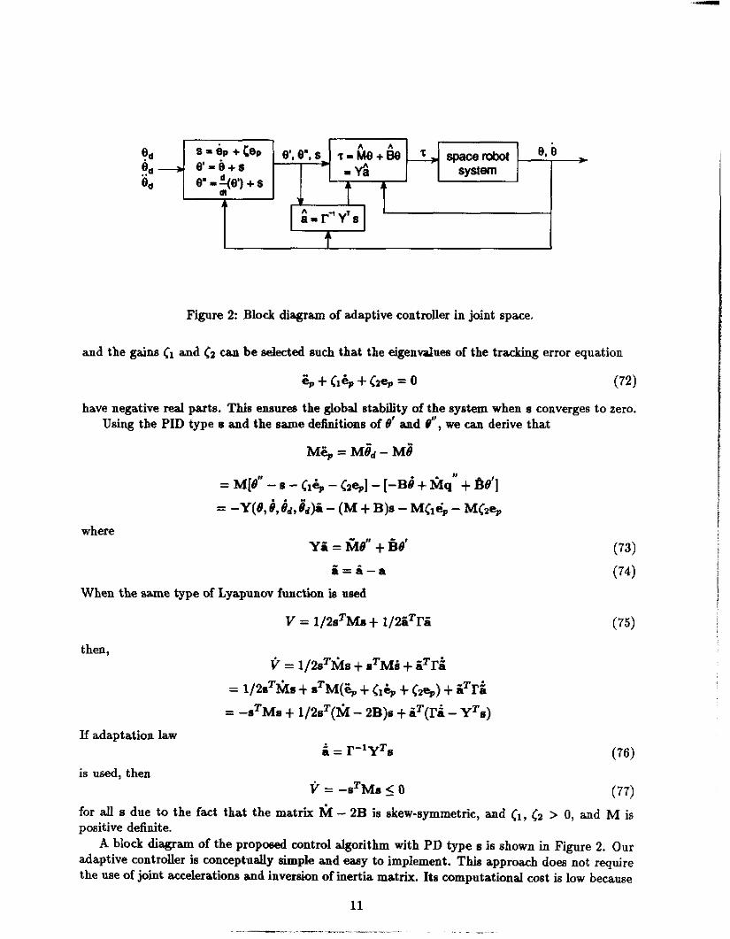
Figure 2 Block diagram of adaptive controller in joint space.

and the gains el and can be selected such that the eigenvalues of the tracking error equation

;a + (1% +ea% = 0 (72)

have negative real parts. This ensures the global stability of the syetem when (I converges to zero. Using the PID type s and the same definitions of 8' and P", we can derive that

M% = Me"d - Me"

= M[8" - s - e+,, - (p+] - [-Bi + Mq + Be'] = -Y(8, i , id,idp - (M t B)8 - M~Ic$ - Mcze,

where y i = fie" + fie'

i=&-a

When the same type of Lyapunov fundion is used

v = 1/2sTMs + 1/2ZTrs

then,

If adaptation law

is used, then

h = r - l y T s

V = -sTMs < 0

(73)

(74)

(75)

(77) for all s due to the fact that the matrix M - 2B is skew-symmetric, and (1, (2 > 0, and M is pmitive definite.

A block diagram of the proposed control algorithm with PD type s is shown in Figure 2. Our adaptive controller is conceptually simple and easy to implement. This approach does not require the use of joint d e r a t i o n s and inversion of inertia matrix. Its computational cost is low because

11

._ ~

it can be implemented through the use of Newton-Euler recursive formulation. It can be seen from Equation (62) which has the same structure as computed torque method, that the control law can be computed efftciently using a Newton-Euler formulation once i have been specified. A high gain feedback is not a must for the system stability. This adaptive approach can also be applied to industrial robot control by a slight modification.

5 Adaptive Control in Inertia Space

In this section, we extend our joint sppoe adaptive control approaches to the problems where control variables are specified in inertia space.

Conceptually, for most applications, the desired robot hand trajectory (i.e., position, velocity and acceleration) must be specified in inertia space. For exampk, let's consider catching a moving object by a space robot. The desired trajectory after catching depends upon the tasks and the motion trajectory of the object More catching, and thus must be specified in inertia space. In other words, as in the case of fixed-base robot tasks are normally specified in Cartesian space, tasks in space applications are unlikely to be specified in joint space. Fortunately, the mapping from robot hand position in inertia space to displacements in joint space can be uniquely determined for space robot system with an nttitude conttolled base, which differs from the case of a completely free-flying space robot system. This unique kinetic relationship has been first studied by Longman et al. [9], and also is illustrated by a planar example in our case study.

However, the unique kinematics relationship UUL only be determined when dynamic parameters are given, for this relationship is indeed dynamic dependent. When some dynamic parameters are unknown, which is indeed the reason why we come to adaptive control, the mapping cannot be determined! Therefore, the primary diEculty of extending our a p p d from Fit space to inertia space is that the desired trajectory in inertia space cannot be transformed to the desired trajectory in joint space because m e dynamic parameters are unknown. In previous discussion, we have utilized a desired trajectory in joint space, as other researchers have done [16], without giving any explanation about how the trajectory is generated, The problem is not significant if the objective is to identify dynamic parameters, but is important if the objective is to control the system.

The problem can be resolved if the same structured adaptive control scheme can be implemented in inertia space. This, however, is not feasible because the proposed adaptive control scheme in joint space req- that the dynamic model must be linearly parameterized. Therefore, the same type of the control scheme cannot be devebped in inertia apace. As has been known, the dynamic related generalized Jacobian of space robot makes it impossible to suitably choose a e t of dynamic parameters such that the inertia space system dynamics can be linearized. That is why the same strnctured adaptive eontrohr in joint space is not feasible for adaptive control in inertia space.

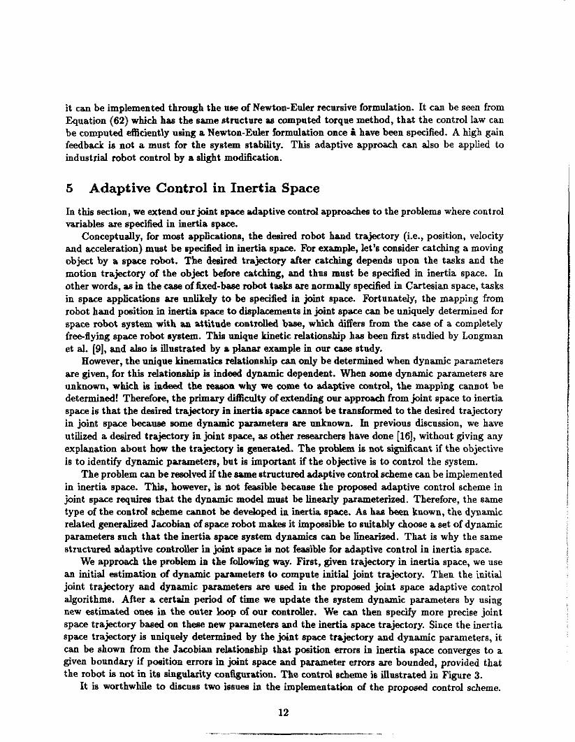
We approach the problem in the following way. First, given trajectory in inertia space, we use an initial estimation of d y n h c parameters to compute initial joint trajectory. Then the initial joint trajectory and dynamic parameters are used in the proposed joint space adaptive control algorithms. After a certain period of time we update the system dynamic parameters by using new athated onea in the outer loop of OUT controller. We can then specify more precise joint space trajectory based on these new parameters and the inertia space trajectory. Since the inertia space trajectory is uniquely determined by the joint space trajectory and dynamic parameters, it can be shown from the Jacobian relatioriship that position errors in inertia space converges to a given boundary if position errors in joint space and parameter errors are bounded, provided that the robot is not in its singularity Eonfiguration. The control scheme is itlustrated in Figure 3.

It is worthwhile to &USS two issues in the implementation of the proposed control scheme.

12

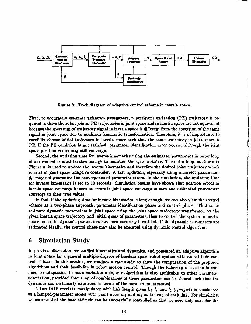
Figure 3: Block diagram of adaptive control d e m e in inertia space.

First, to accurately estimate unLnown parameters, a persistent excitation (PE) trajectory is re- quired to drive the robot joints. PE trajectories in joint space and in inertia space are not equivalent because the spectrum of trajectory Signal in inertia space is Merent from the spectrum of the same signal in joint space due to nonlinear kinematic transformation. Therefore, it is of importance to carefully choose initial trajectory in inertia space such that the same trajectory in joint space is PE. If the PE condition in not satisfied, parameter identification error occurs, although the joint space position errors may still converge.

Second, the updating time for inverse kinemati- using the estimated parameters in outer loop of our controller must be slow enough to maintain the system stable. The outer loop, as shown in Figure 3, is used to update the in- kinematics and therefore the desired joint trajectory which is used in joint space adaptive controller. A fast updation, especially using incorrect parameters fi<, may not guarantee the convergence of parameter errors. In the simulation, the updating time for inverse kinematics is set to 10 seooads. Simulation reeults have shown that p i t i o n errors in inertia space converge to zero a8 errors in joint space converge to aepo and estimated parameters converge to their true valua.

In fact, if the updating time for inverse kinematics in long enough, we can also view the control scheme as a two-phase a p p d , parameter identification phase and control phase. That is, to estimate dynamic parametera in joint space U s i n g the joint space trajectory transformed by the given inertia s p a trajectory and initial guess of parameters, then to control the system in inertia space, once the dynamic parameters has been correctly identified. If the dynamic parameters are estimated ideally, the control phase may also be executed using dynamic control algorithm.

6 Simulation Study In previous discussion, we studied kinematics and dynamics, and presented an adaptive algorithm in joint space for a general multipl+degmes-of-freedom space robot system with an attitude con- trolled base. In this section, we conduct a case study to show the computation of the proposed algorithms and their feasibility in robot motion control. Though the following discussion is con- fined to adaptation to mass variation only, our algorithm is also applicable to other parameter adaptation, provided that a set of combmations of those parameters ran be chosed such that the dynamics can be linearly expresaed in terms of the parameters interested.

A tweDOF revolute manipulator with link length given by l1 and 11 (11=12=1) is considered as a lumped-parameter model with point mas8 ml and rnl at the end of each link. For simplicity, we assume that the base attitude can be successfully controlled 80 that we need only consider the

13

Base

Y

L ZI

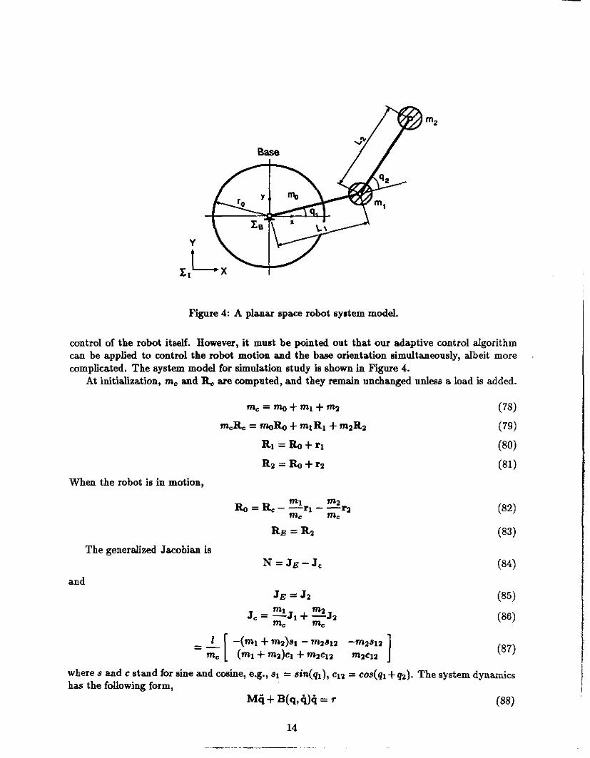
Figure 4: A planar space robot system model.

control of the M It itself. However, it must be pointed out that our adaptive contrc algorithm can be applied to control the robot motion and the base orientation Bimultaneously, albeit more complicated. The system model for simulation study is shown in F i i 4.

At initialization, m. and R, are computed, and they remain unchanged unleas a load is added.

,

mc = m0S ml + m2

m.R. = mo% + mlRl + m z ~ z

RI = Bo + rl

R z = R o + r a When the robot is in motion,

The generalized Jacobian is

and

where B and c stand for sine and wine , e.g., 81 = sin(ql), c1z = cos(ql +q2). The system dynamics has the following form,

Mi + B(q,G)G = r (88)

14 _- ..

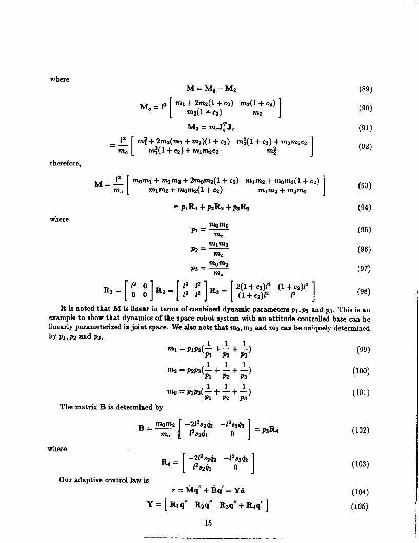
where

therefore,

where

It is noted that M is linear in terms of combined dynamic parameters n,p1 and p3. This is an example to show that dynamics of the space robot system with an attitude controlled base can be linearly parameterized in joint space. We ale0 note that mo, ml and mz can be uniquely determined by P l , n and P 3 1

1 1 1 m1= Pm(- + - + -) mz = mm(- + - + -)

m n P 3 1 1 1

n 4 m 1 1 1 n n P 3

mo = nm(- + - + -1 The matrix B is determined by

where

Our adaptive control law i~ r = Mq" +Bn' = Yi

Y = [ Riq" lbq" R3q" + R4q' ] 15

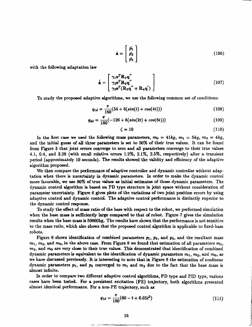
with the following adaptation law

To study the proposed adaptive algorithms, we use the following common set of conditions:

In the first case we used the following maas parametera, n h ~ = 41kg, ml = 5kg, m2 = 4kg, and the initial guess of all three parameters is set to 50% of their true values. It can be found from Figure 5 that joint errors converge to zero and all parameters converge to their true values 4.1, 0.4, and 3.28 (with small relative errors 12%, 2.1%, 2.5%, respectively) after a transient period (approximately 10 seconds). The results showed the validity and efficiency of the adaptive algorithm proposed.

We then compare the performance of adaptive controller and dynamic controller without adap- tation when there is uncertainty in dynamic parameters. In order to make the dynamic control more favorable, we use 80% of true d u e s as initial estimates of those dynamic parameters. The dynamic control algorithm is based on PD type structure in Fit space without consideration of parameter uncertainty. Figure 6 given plots of the variations of two joint position errors by using adaptive control and dynamic control. The adaptive contrd performance is distinctly superior to the dynamic control response.

To study the dect of mass ratio of the base with respect to the robot, we performed simulation when the base mass is sufficiently large compared to that of robot. Figure 7 gives the simulation results when the base maas is 5M)oOkg. The results have shown that the performance is not sensitive to the mass ratio, which also shows that the pro@ control algorithm is applicable to fixed-base robots.

Figure 8 shows identification of combined parameters m, pz, and PJ, and the resultant mass ml, m, and nh~, in the above case. From Figure 8 we found that estimation of aJl parameters mi, mz, and m~ are very dose to their true values. This demonatrated that identification of combined dynamic parameters is equivalent to the identifieation of dynamic parameters ml, ml, and m, as we have discussed PreViOUdy. It in interesting to note that in Figure 8 the estimation of nonlinear dynamic parameters fir and pj converged to ml and rnz due to the fact that the base mass is almost infinite.

In order to compare two different adaptive control algorithms, PD type and PID type, various cases have been tested. For a persistent excitation (PE) trajectory, both algorithms presented almost identical performance. For a non-PE trajectory, such as

r a d = -(60 - t t 0.05P) 180

16

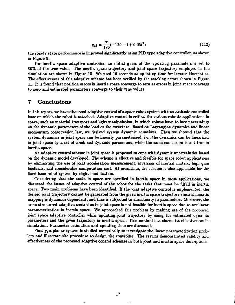
the steady state performance is improved significantly using PID type adaptive controller, as shown in Figure 9.

For inertia space adaptive contrdler, an initid guess of the updating parameters is set to 80% of the true value. The inertia space trajectory and joint space trajectory employed in the simulation are shown in Figure 10. We used 10 seconds as updating time for inverse kinematics. The effectiveness of this adaptive scheme has been verified by the tracking errors shown in Figure 11. It is found that position errors in inertia space converge to rn as errors in joint space converge to zero and estimated parameters converge to their true value8.

7 Conclusions In this report, we have discussed adaptive controlof a space robot system with an attitude controlled base on which the robot is attached. Adaptive control is critical for Various robotic applications in space, such as m a t d tramport and light manipulation, in which robots have to face uncertainty on the dynamic parameters of the load or the structure. Bared on Lagrangian dynamics and linear momentum conservation law, we derived system dynamic equations. Then we showed that the system dynamica in pint space can be linearly parameterized, Le., the dynamics can be linearized in joint space by a set of combined dynamic parameters, while the same conclusion is not true in inertia space.

An adaptive control scheme in joint space is proposed to cope with dynamic uncertainties based on the dynamic model developed. The scheme is effective and feasible for space robot applications by eliminating the we of pint acceleration measurement, inversion of inertial matrix, high gain feedback, and considerable computation cost. At meantime, the scheme is also applicable for the iixed-base robot system by slight modification.

Considering that the tasks in space are specified in hertia space in most applicationa, we discussed the issues of adaptive control of the robot for the tasks that must be mull in inertia space. Two main problems have been identified. If the pint adaptive control is implemented, the desired joint trajectory cannot be generated from the given inertia space trajectory since kinematic mapping is dynamics dependent, and thus is subjected to uncertainty in parameters. Moreover, the same structured adaptive control as in joint space is not feasible for inertia space due to nonlinear parameterization in inertia space. We approached this problem by making use of the proposed joint space adaptive controller while updating joint trajectory by using the estimated dynamic parameters and the given trajectory in inertia space. This method has shown its effectiveness in simulation. Parameter estimation and updating time are direussed.

Finally, a planar system is studied numerically to investigate the linear parameterization prob- lem and illustrate the procedure to design the controller. The results demonstrated validity and effectiveness of the proposed adaptive control schemes in both joint and inertia space descriptions.

17

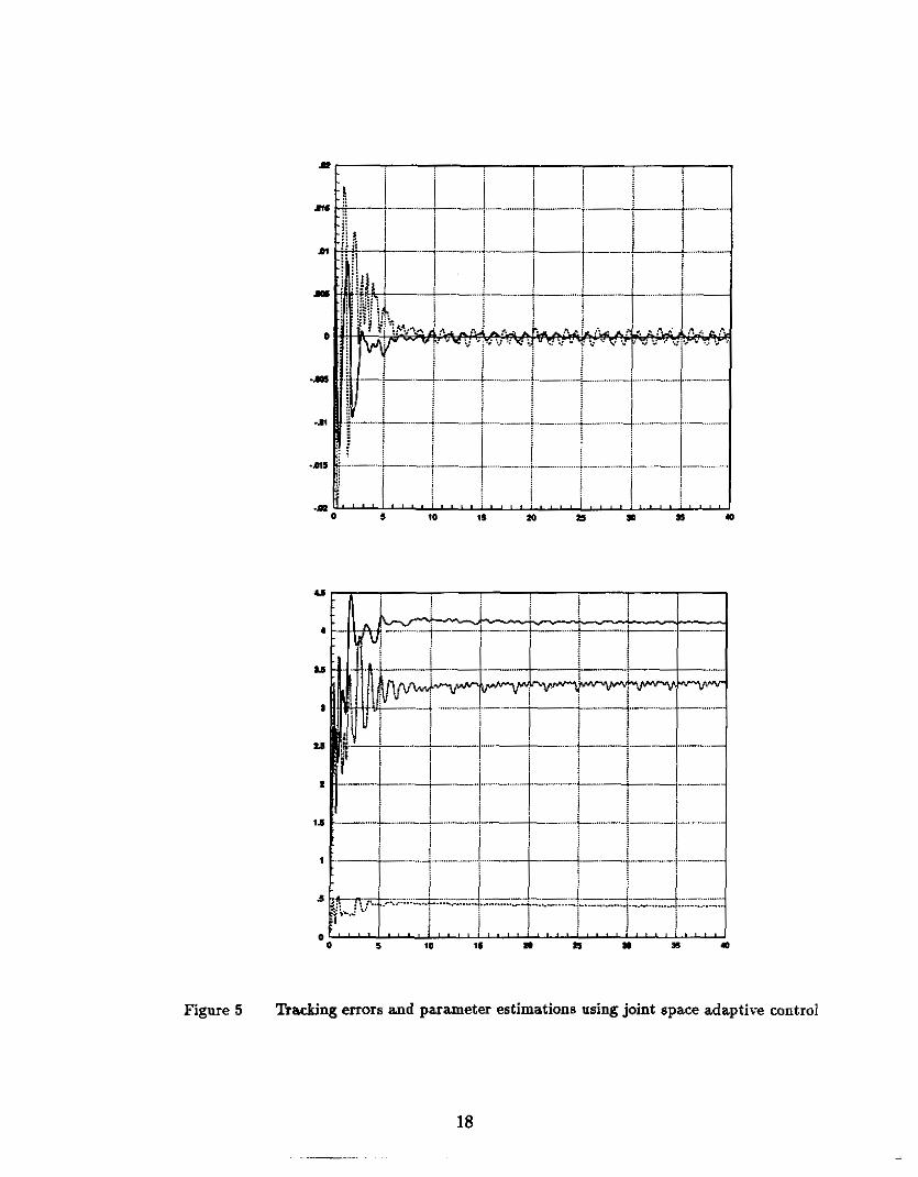
Figure 5 'Racking errors and parameter estimations using joint space adaptive control

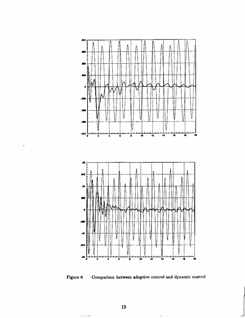
Figure 6 Comparison between adaptive control and dynamic control

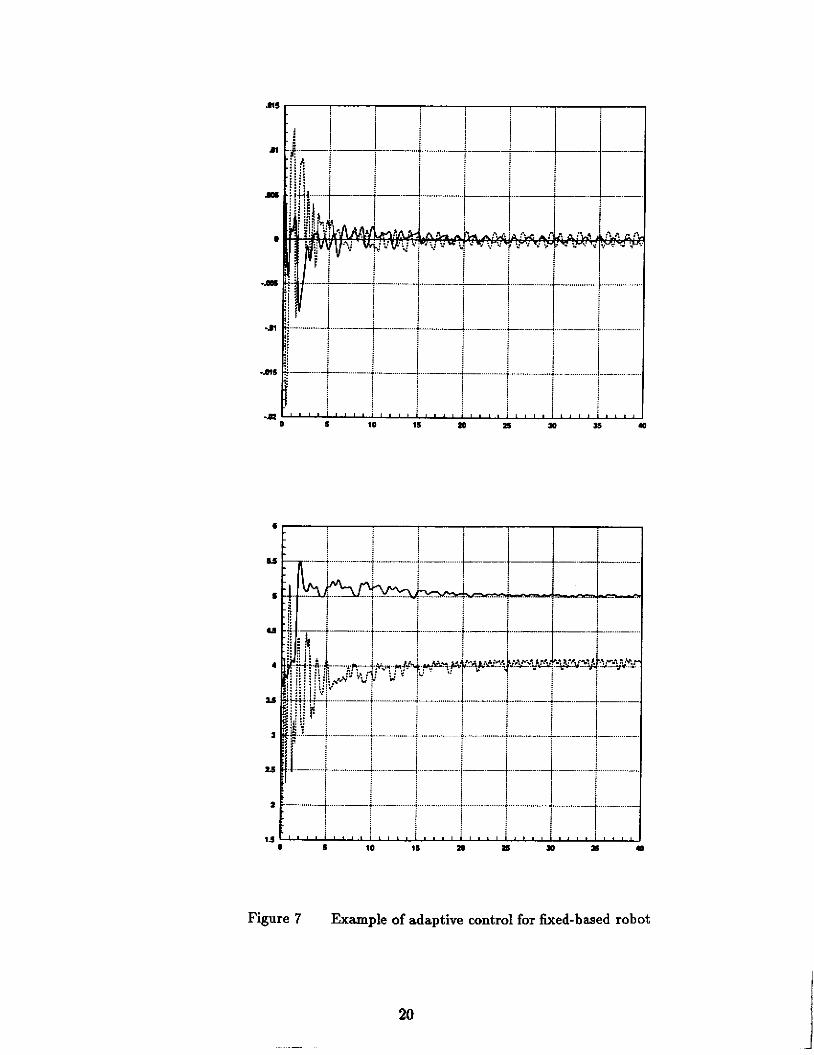
Figure 7 Example of adaptive control for fixed-based robot

20

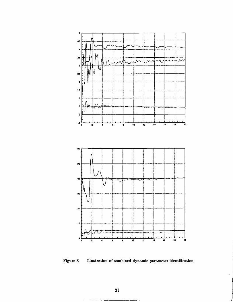
Figure 8 Illustration of combined dynamic parameter identification

21

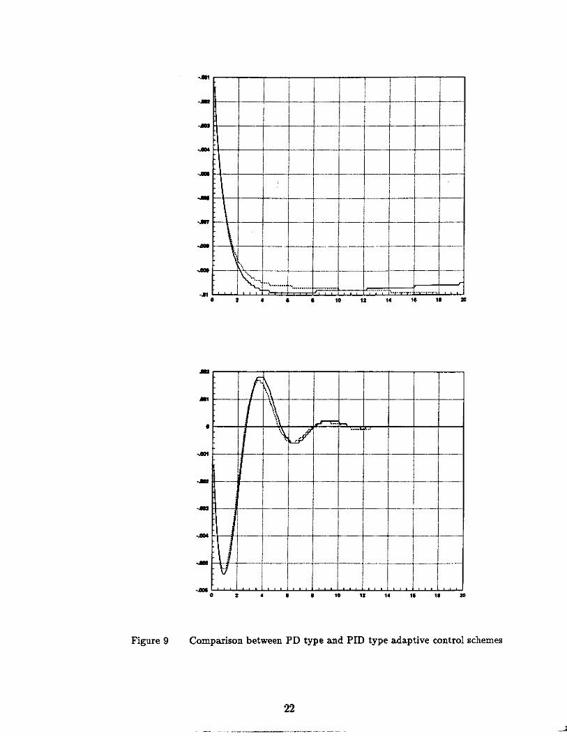
Figure 9 Comparison between PD type and PID type adaptive control schemes

22

- .

6 10 W S a

5 i a n a I

Figure 10 Trajectories in joint space and in inertia space using inertia space adaptive controller

0 6 W S m a

Figure 11 Thcking errors in joint space and in inertia space using inertia space adaptive controller

23

References

[l] A.K. Bejcay and B. Hannaford. Man-machine interaction in space telerobotics. In Proceedings of the International Syrnpoukrn of Telmpemtion and m t d 1988, 1988.

[2] J.J Craig, P. Hsu, and S.S. Sastry. Adaptive control of mechanical manipulators. International Journal of Robotics Research, 6(2), 1987.

[3] S. Dubowsky and D. DeuFoges. The application of model-referenced adaptive control to robotic manipulators. ASME Journal of Dylamic Sgstem, Meawurement, and Contml, 1979.

(41 G. Butler (edited). The dfst century in spoce: adavances in the astmunticnlsciences. American Astronautical Society, 1988.

[5] R. Homwite and M. Tomizuka. An adaptive control scheme for mechanical manipulators. In ASME Paper No. 80- WA/LSC-6,1980.

[6] J.L. Junkins. Mechanics and codd of laqe peZible etrucluws. American Institute of Aero- nautics and Astronautics, 1990.

[7] 0. Khatib, J.J. Craig, and T. Lozano-Perez. The mbolics review. MIT Press, 1989.

[SI P. Khosla and T. h a d e . Parameter identification of robot dynamics. In Proceedings of IEEE International Conferenoe on Decision and Contml, 1885.

[9] R.W. Longman, R.E. Lindberg, and M.F. Zadd. Satellitemounted robot manipulators: new kinematics and reaction moment compensation. International Journal of Robties Research, 6(3), 1987.

[lo] R.H. Middleton and G.C. Goodwin. Adaptive computed torque control for rigid link manip- ulators. In Pmcdinge of IEEE International Conferem on Decieion and Contml, 1986.

[11] J.J. Slotine and W. Li. On the adaptive control of robot manipulators. International Journal of Robotics Research, 6(3), 1987.

[12] J.J. Slotine and W. Li. Applied nonlinear contml. New Jersey: Printice H d , 1991.

113) M.W. Spong and M. Vidyasagar. Robot dynamics and control. John Wiley & Sons, 1989.

(141 H. Ueno, Y. Xu, and et al. On control and planning of a apace robot walker. In Proceedings of 1990 IEEE International conference on System engineering, 1990.

[15] M. U h a n and R. Cannon. Experiments in global navigation and control of freeflying space robot. In proaeedings of ASME Winter Conferem, 1989.

(161 M.W. WaIker and GB. Wee. An adaptive control strategyfor space based robot manipulators.

[17] W.L. Whittaker and T. Kanade. Spoce robotics in J a p n . Loyola college, 1991.

In Ptvoxdinge of IEEE Conference on Robotics and Automation, 1991.