This content has been downloaded from IOPscience. Please scroll down to see the full text.

Download details:

IP Address: 193.170.138.151

This content was downloaded on 30/09/2014 at 13:33

Please note that terms and conditions apply.

Adaptive evolution of molecular phenotypes

View the table of contents for this issue, or go to the journal homepage for more

J. Stat. Mech. (2014) P09029

(http://iopscience.iop.org/1742-5468/2014/9/P09029)

Home Search Collections Journals About Contact us My IOPscience

J. Stat. M

ech. (2014) P09029

ournal of Statistical Mechanics:J Theory and Experiment

Adaptive evolution of molecularphenotypes

Torsten Held1, Armita Nourmohammad1,2 andMichael Lassig1

1 Institut fur Theoretische Physik, Universitat zu Koln, Zulpicherstr. 77,50937, Koln, Germany

2 Joseph Henry Laboratories of Physics and Lewis-Sigler Institute forIntegrative Genomics, Princeton University, Princeton, NJ 08544, USA

E-mail: mlaessig@uni-koeln.de

Received 20 March 2014Accepted for publication 13 July 2014Published 30 September 2014

Online at stacks.iop.org/JSTAT/2014/P09029doi:10.1088/1742-5468/2014/09/P09029

Abstract. Molecular phenotypes link genomic information with organismicfunctions, fitness, and evolution. Quantitative traits are complex phenotypesthat depend on multiple genomic loci. In this paper, we study the adaptiveevolution of a quantitative trait under time-dependent selection, which arisesfrom environmental changes or through fitness interactions with other co-evolvingphenotypes. We analyze a model of trait evolution under mutations and geneticdrift in a single-peak fitness seascape. The fitness peak performs a constrainedrandom walk in the trait amplitude, which determines the time-dependenttrait optimum in a given population. We derive analytical expressions for thedistribution of the time-dependent trait divergence between populations andof the trait diversity within populations. Based on this solution, we developa method to infer adaptive evolution of quantitative traits. Specifically, we showthat the ratio of the average trait divergence and the diversity is a universalfunction of evolutionary time, which predicts the stabilizing strength and thedriving rate of the fitness seascape. From an information-theoretic point of view,this function measures the macro-evolutionary entropy in a population ensemble,which determines the predictability of the evolutionary process. Our solution alsoquantifies two key characteristics of adapting populations: the cumulative fitness

Content from this work may be used under the terms of the Creative Commons Attribution3.0 licence. Any further distribution of this work must maintain attribution to the author(s)

and the title of the work, journal citation and DOI.

c© 2014 IOP Publishing Ltd and SISSA Medialab srl 1742-5468/14/P09029+39$33.00

J. Stat. M

ech. (2014) P09029

Adaptive evolution of molecular phenotypes

flux, which measures the total amount of adaptation, and the adaptive load,which is the fitness cost due to a population’s lag behind the fitness peak.

Keywords: driven diffusive systems (theory), evolutionary and comparativegenomics (theory), models for evolution (theory), population dynamics (theory)

Contents

1. Introduction 3

2. Evolutionary dynamics of quantitative traits 52.1. Diffusion equations for trait mean and diversity . . . . . . . . . . . . . . . . . . . . . . . . . . . . . 52.2. Stochastic seascape models . . . . . . . . . . . . . . . . . . . . . . . . . . . . . . . . . . . . . . . . . . . . . . . . . 92.3. Joint dynamics of trait and selection . . . . . . . . . . . . . . . . . . . . . . . . . . . . . . . . . . . . . . . 112.4. Discussion . . . . . . . . . . . . . . . . . . . . . . . . . . . . . . . . . . . . . . . . . . . . . . . . . . . . . . . . . . . . . . . . . 12

3. Adaptive evolution in a single-peak fitness seascape 133.1. Stationary distribution of mean and optimal trait . . . . . . . . . . . . . . . . . . . . . . . . . . . 133.2. Time-dependent trait divergence . . . . . . . . . . . . . . . . . . . . . . . . . . . . . . . . . . . . . . . . . . . 173.3. Stationary trait diversity . . . . . . . . . . . . . . . . . . . . . . . . . . . . . . . . . . . . . . . . . . . . . . . . . . . 203.4. Discussion . . . . . . . . . . . . . . . . . . . . . . . . . . . . . . . . . . . . . . . . . . . . . . . . . . . . . . . . . . . . . . . . . 21

4. Fitness and entropy of adaptive processes 234.1. Genetic load . . . . . . . . . . . . . . . . . . . . . . . . . . . . . . . . . . . . . . . . . . . . . . . . . . . . . . . . . . . . . . . 234.2. Fitness flux . . . . . . . . . . . . . . . . . . . . . . . . . . . . . . . . . . . . . . . . . . . . . . . . . . . . . . . . . . . . . . . . 254.3. Predictability and entropy production . . . . . . . . . . . . . . . . . . . . . . . . . . . . . . . . . . . . . . 274.4. Discussion . . . . . . . . . . . . . . . . . . . . . . . . . . . . . . . . . . . . . . . . . . . . . . . . . . . . . . . . . . . . . . . . . 27

5. Inference of adaptive trait evolution 285.1. Statistics of the divergence-diversity ratio Ω . . . . . . . . . . . . . . . . . . . . . . . . . . . . . . . . 295.2. The Ω test for stabilizing and directional selection . . . . . . . . . . . . . . . . . . . . . . . . . . 305.3. Comparison with sequence-based inference of selection . . . . . . . . . . . . . . . . . . . . . . 31

6. Conclusion 32

Appendix A. Analytical theory of the adaptive ensemble 32A.1. Moments of the optimal trait . . . . . . . . . . . . . . . . . . . . . . . . . . . . . . . . . . . . . . . . . . . . . . . 33A.2. Moments of the trait mean . . . . . . . . . . . . . . . . . . . . . . . . . . . . . . . . . . . . . . . . . . . . . . . . . 33A.3. Propagators . . . . . . . . . . . . . . . . . . . . . . . . . . . . . . . . . . . . . . . . . . . . . . . . . . . . . . . . . . . . . . . . 34

Appendix B. Numerical simulations 35

References 37

doi:10.1088/1742-5468/2014/09/P09029 2

J. Stat. M

ech. (2014) P09029

Adaptive evolution of molecular phenotypes

1. Introduction

This is the second in a series of papers on the evolution of quantitative traits inbiological systems [1]. We focus on molecular traits such as protein binding affinitiesor gene expression levels, which are mesoscopic phenotypes that bridge between genomicinformation and higher-level organismic traits. Such phenotypes are complex: they dependon tens to hundreds of constitutive genomic sites and are generically polymorphic in apopulation. Moreover, their evolution is often a strongly correlated process that involveslinkage disequilibrium, i.e. allele associations due to incomplete recombination, andepistasis, i.e. fitness interactions, between constitutive sites. Hence, the evolutionarystatistics of molecular quantitative traits have to go beyond traditional quantitativegenetics [2–11]. Our aim is to derive universal phenotypic features of these processes, whichdecouple from details of a trait’s genomic encoding and of the molecular evolutionarydynamics.

In this paper, we focus on the adaptive evolution of molecular traits, which involvesmutations, genetic drift, and (partial) recombination of the trait loci. The adaptivedynamics take place on macro-evolutionary time scales and can generate large traitchanges—in contrast to micro-evolutionary processes based on standing trait variationin a population. Adaptive trait changes are driven by time-dependent selection on thetrait values. Specifically, we consider the trait evolution in a single-peak fitness seascape[12–14], which has a moving peak described by a stochastic process in the trait coordinate.The time-dependence of the optimal trait value can have extrinsic or intrinsic causes; forexample, the optimal expression level of a gene is affected by changes in the environmentof an organism and by expression changes of other genes in the same gene network. Thesefitness seascape models have two fundamental parameters: the stabilizing strength and thedriving rate, which measure the width and the mean square displacement of the fitnesspeak per unit of evolutionary time. In an ensemble of populations with independentfitness peak displacements, these dynamics describe lineage-specific adaptive pressure.We discuss specific seascape models with continuous or punctuated adaptive pressure;that is, the fitness peak performs a constrained (Ornstein–Uhlenbeck) random walk or aPoisson jump process in the trait coordinate. These stochastic processes define minimalnon-equilibrium models for the adaptive evolution of a quantitative trait.

Here we focus on macro-evolutionary fitness seascapes, which have low driving ratescompared to the diffusion of the trait by genetic drift and describe persistent selection on aquantitative trait [12,15]. We show that this kind of selection generates two complementaryevolutionary forces. On short time scales, a single fitness peak acts as stabilizing selection,which constrains the trait diversity within a population as well as its divergence betweenpopulations. On longer time scales, the population trait mean follows the moving fitnesspeak, which generates an adaptive component of the trait divergence. In the limit case ofa static fitness landscape, we recover the evolutionary equilibrium of quantitative traitsunder stabilizing selection, which has been the subject of a previous publication [1]. Theevolution in a quadratic fitness landscape is described by an Ornstein-Uhlenbeck dynamicsof the trait mean [16–19], which should not be confused with the Ornstein-Uhlenbeckprocess of the fitness peak in a stochastic seascape.

doi:10.1088/1742-5468/2014/09/P09029 3

J. Stat. M

ech. (2014) P09029

Adaptive evolution of molecular phenotypes

We also discuss the regime of micro-evolutionary fitness seascapes, which describerapidly changing selection on a quantitative trait. Such fitness changes are ubiquitouslygenerated by ecological fluctuations. They lead to micro-evolutionary adaptation ofthe trait from its standing variation in a population but do not generate directionalselection on evolutionary time scales. We show that micro-evolutionary fitness seascapescan be mapped to effective fitness landscapes that describe relaxed stabilizingselection.

Our model of adaptive trait evolution contains different sources of stochasticity:mutations establish trait differences between individuals within one population,reproductive fluctuations (genetic drift) and fitness seascape fluctuations generate traitdifferences between populations with time. In macro-evolutionary fitness seascapes, thesestochastic forces act on different time scales and define different statistical ensembles,similar to thermal and quenched fluctuations in the statistical thermodynamics ofdisordered systems. In section 2, we derive stochastic evolution equations for the traitmean, the trait diversity, and the position of the fitness peak, which establish a jointdynamical model for the trait and the underlying fitness seascape over macro-evolutionarytime-scales. In section 3, we discuss the analytical solution of these models for a stationaryensemble of adapting populations. This ensemble has a time-independent trait diversitywithin populations, as well as a trait divergence between populations that depends ontheir divergence time. In section 4, we evaluate two important summary statistics ofadaptive processes. The genetic load, which is defined as the difference between themaximum fitness and the mean population fitness, is shown to include a specific adaptivecomponent, which results from the lag of the population behind the moving fitnesspeak. The cumulative fitness flux measures the amount of adaptation in a populationover a macro-evolutionary period: it is zero at evolutionary equilibrium and increasesmonotonically with the driving rate of selection [20]. Furthermore, we determine thepredictability of trait values in one population given its distribution in another population,which is given by a suitably defined entropy of the population ensemble under divergentevolution.

The statistical theory of this paper provides a new method to infer selection on aquantitative trait from diversity and time-resolved divergence data. Given these data in afamily of evolving populations, we use the divergence-diversity ratio Ω(τ) for differentdivergence times τ to determine the stabilizing strength and the driving rate of theunderlying fitness seascape. These selection parameters, in turn, quantify the amount ofconservation and adaptation in the evolution of the trait. The divergence-diversity ratio isuniversal: it depends on the stabilizing strength and the driving rate of the fitness seascapeas well as on the evolutionary distance between populations, but it is largely independentof the trait’s constitutive sites, of the amount of recombination between these sites, andof the details of the fitness dynamics. In contrast to most sequence evolution tests, theΩ test does not require the gauge of a neutrally evolving ‘null trait’. We discuss this testalong with probabilistic extensions in section 5.

This paper contains some necessarily technical derivations of our main results. Forreaders who are not interested in technical issues, it offers a fast track: the sectionsummaries 2.3, 3.4 and 4.4, the description of the Ω test in section 5, and the concludingsection 6 can be read as a self-contained unit.

doi:10.1088/1742-5468/2014/09/P09029 4

J. Stat. M

ech. (2014) P09029

Adaptive evolution of molecular phenotypes

2. Evolutionary dynamics of quantitative traits

In this section, we develop minimal models for the adaptive evolution of quantitativetraits in a fitness seascape. We first review the diffusion dynamics for the trait meanand the diversity under genetic drift and mutations in a given fitness landscape, whichhave been derived in a previous paper [1]. Second, we introduce simple stochastic modelsfor the dynamics of selection, which promote fitness landscapes to fitness seascapes. Wethen combine the dynamics of trait and selection to a joint, non-equilibrium evolutionarymodel.

2.1. Diffusion equations for trait mean and diversity

Our model for quantitative traits is based on a simple additive map from genotypes tophenotypes. The trait value E of an individual depends on its genotype a = (a1, . . . , a�)at � constitutive genomic sites,

E(a) =�∑

i=1

Eiσi, with σi ≡{

1, if ai = a∗i ,

0, otherwise. (1)

Here, the trait is measured from its minimum value, and Ei > 0 is the contribution of agiven site i to the trait value. We assume a two-allele genomic alphabet and a∗

i denotesthe allele conferring the larger phenotype at site i. The extension to a four-allele alphabetis straightforward. The genotype-phenotype map (1) defines the allelic trait average Γ0

and the trait span E20 ,

Γ0 =12

�∑i=1

Ei, E20 =

14

�∑i=1

E2i . (2)

The linear genotype-phenotype map (1) has been chosen here for concreteness. Suchlinear maps are approximately realized for some molecular traits, such as transcriptionfactor binding energies [21]. However, many other systems have nonlinearities, which arecommonly referred to as trait epistasis. It can be argued that simple forms of trait epistasiswill leave many of our results intact (this is indicated at a few places in the manuscript),but a systematic inclusion of trait epistasis is beyond the scope of this paper. At the sametime, the fitness land- and seascapes introduced below depend on the trait in a nonlinearway; hence, they always contain fitness epistasis.

Quantitative traits have a sufficient number of constitutive loci to be genericallypolymorphic in a population, although most individual genomic sites are monomorphic.The distribution of trait values in a given population, W(E), is often approximatelyGaussian [1, 3, 14]. Hence, it is well characterized by its mean and variance,

Γ ≡ E =∫

dE E W(E),

Δ ≡ (E − Γ )2 =∫

dE (E − Γ )2 W(E), (3)

doi:10.1088/1742-5468/2014/09/P09029 5

J. Stat. M

ech. (2014) P09029

Adaptive evolution of molecular phenotypes

where overbars denote averages over the trait distribution W(E) within a population.The variance Δ will be called the trait diversity; in the language of quantitative genetics,this quantity equals the total heritable variance including epistatic effects.

We consider the evolution of the trait E under genetic drift, genomic mutations,and natural selection, which is given by a trait-dependent fitness seascape f(E, t) thatchanges on macro-evolutionary time scales. This process is illustrated in figure 1: At agiven evolutionary time, the trait distribution in a population has mean Γ (t), diversityΔ(t), and is positioned at a distance Λ(t) ≡ Γ (t) − E∗(t) from the optimal trait value.The trait distribution follows the moving fitness peak, building up a trait divergence

D(1)(t, τ) = (Γ (t) − Γ (t − τ))2 (4)

between an ancestral population at time t−τ and its descendent population at time t in agiven lineage. In the same way, we can define the trait divergence between two descendentpopulations at time t that have evolved independently from a common ancestor populationat time t − τ/2,

D(2)(t, τ) = (Γ1(t) − Γ2(t))2. (5)

In a suitably defined ensemble of parallel-evolving populations, the expectation valuesof these divergences, 〈D(κ)(τ)〉 (κ = 1, 2), depend only on the divergence time τ . Theasymptotic divergence for long times is just twice the trait variance across populations,

limτ→∞

〈D(κ)(τ)〉 = 2〈(Γ − 〈Γ 〉)2〉 (κ = 1, 2). (6)

In particular, the quantity E20 defined in (2) is the trait variance in an ensemble of

random genotypes, which results from neutral evolution (with averages 〈. . .〉0 marked bya subscript) at low mutation rates, E2

0 = limμ→0〈(Γ − 〈Γ 〉0)2〉0. For finite times, however,the statistics of the single-lineage divergence D(1) and the cross-lineage divergence D(2)

differ from each other in an adaptive process. As we will discuss in detail below, thisis a manifestation of the non-equilibrium evolutionary dynamics in a fitness seascape. Incontrast, evolutionary equilibrium in a fitness landscape dictates 〈D(1)(τ)〉eq = 〈D(2)(τ)〉eq

by detailed balance.As shown in a previous companion paper [1], the evolutionary dynamics of a

quantitative trait in a fitness seascape can be described in good approximation by diffusionequations for its mean and its diversity,

∂

∂tQ(Γ , t|F1) =

[gΓΓ

2N∂2

∂Γ 2 − ∂

∂Γ

(mΓ + gΓΓ ∂F1(Γ , t)

∂Γ

)]Q(Γ , t|F1), (7)

∂

∂tQ(Δ, t|F2) =

[gΔΔ

2N∂2

∂Δ2 − ∂

∂Δ

(mΔ + gΔΔ∂F2(Δ, t)

∂Δ

)]Q(Δ, t|F2), (8)

which are projections of the Kimura diffusion equation [22, 23] from genotypes ontothe phenotype space. The distributions Q(Γ , t | F1) and Q(Δ, t | F2) are time-dependentprobability densities of trait mean and variance, which describe an ensemble of populationsevolving in the same fitness seascape f(E, t). These dynamics involve the fitness seascapecomponents

F1(Γ , t) = f(Γ , t) + f ′′(Γ , t) ×∫

dΔΔQ(Δ, t | F2), (9)

doi:10.1088/1742-5468/2014/09/P09029 6

J. Stat. M

ech. (2014) P09029

Adaptive evolution of molecular phenotypes

(a)

(b) (c) (d)

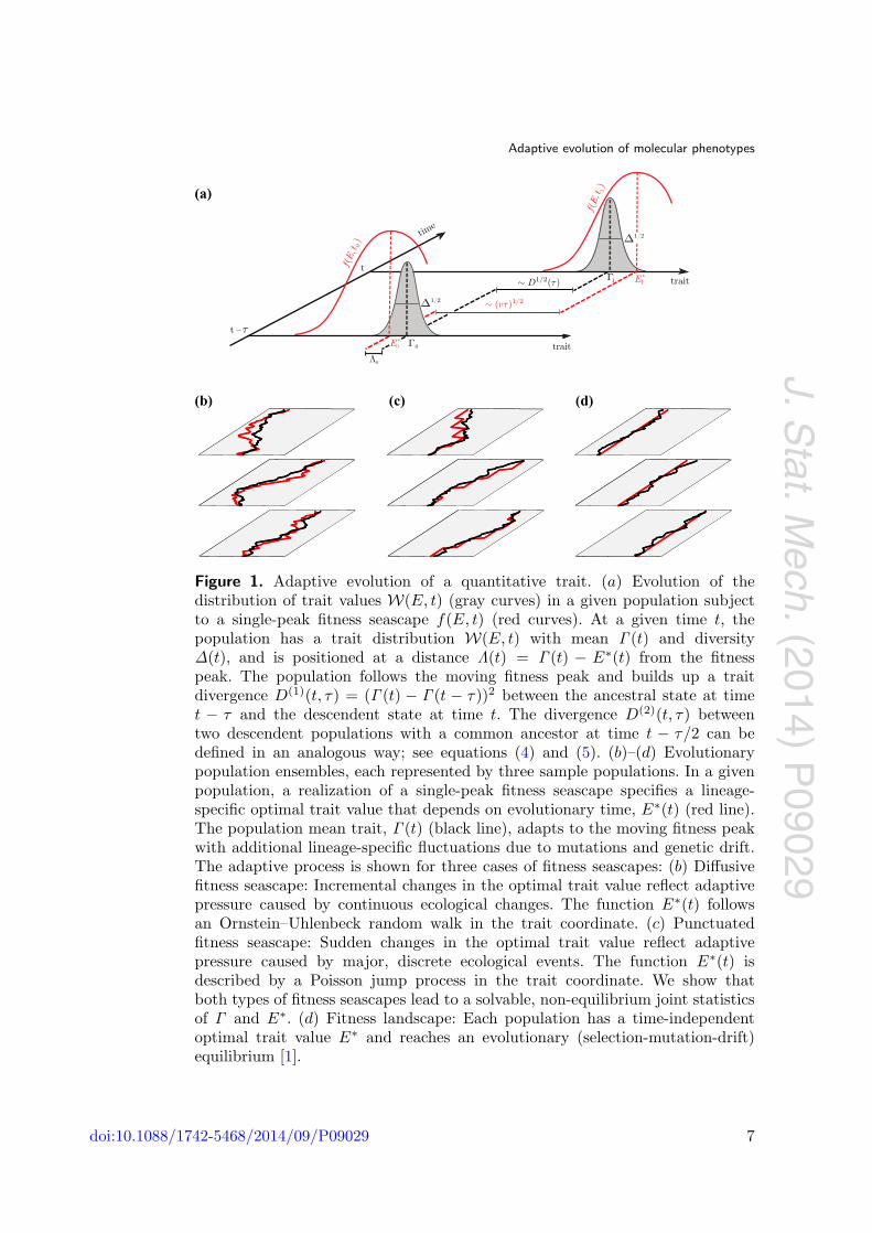
Figure 1. Adaptive evolution of a quantitative trait. (a) Evolution of thedistribution of trait values W(E, t) (gray curves) in a given population subjectto a single-peak fitness seascape f(E, t) (red curves). At a given time t, thepopulation has a trait distribution W(E, t) with mean Γ (t) and diversityΔ(t), and is positioned at a distance Λ(t) = Γ (t) − E∗(t) from the fitnesspeak. The population follows the moving fitness peak and builds up a traitdivergence D(1)(t, τ) = (Γ (t) − Γ (t − τ))2 between the ancestral state at timet − τ and the descendent state at time t. The divergence D(2)(t, τ) betweentwo descendent populations with a common ancestor at time t − τ/2 can bedefined in an analogous way; see equations (4) and (5). (b)–(d) Evolutionarypopulation ensembles, each represented by three sample populations. In a givenpopulation, a realization of a single-peak fitness seascape specifies a lineage-specific optimal trait value that depends on evolutionary time, E∗(t) (red line).The population mean trait, Γ (t) (black line), adapts to the moving fitness peakwith additional lineage-specific fluctuations due to mutations and genetic drift.The adaptive process is shown for three cases of fitness seascapes: (b) Diffusivefitness seascape: Incremental changes in the optimal trait value reflect adaptivepressure caused by continuous ecological changes. The function E∗(t) followsan Ornstein–Uhlenbeck random walk in the trait coordinate. (c) Punctuatedfitness seascape: Sudden changes in the optimal trait value reflect adaptivepressure caused by major, discrete ecological events. The function E∗(t) isdescribed by a Poisson jump process in the trait coordinate. We show thatboth types of fitness seascapes lead to a solvable, non-equilibrium joint statisticsof Γ and E∗. (d) Fitness landscape: Each population has a time-independentoptimal trait value E∗ and reaches an evolutionary (selection-mutation-drift)equilibrium [1].

doi:10.1088/1742-5468/2014/09/P09029 7

J. Stat. M

ech. (2014) P09029

Adaptive evolution of molecular phenotypes

F2(Δ, t) = Δ ×∫

dΓ f ′′(Γ , t) Q(Γ , t | F1), (10)

which are projections of the mean population fitness

f(t) ≡∫

dE f(E, t) W(E, t) = f(Γ , t) +12Δf ′′(Γ , t) + . . . (11)

onto the marginal variables Γ and Δ. Genetic drift enters through the diffusion coefficients

gΓΓ = 〈Δ〉 ≡∫

dΔΔQ(Δ, t | F2), gΔΔ = 2Δ2, (12)

mutations through the mutation coefficients

mΓ = −2μ(Γ − Γ0), mΔ = −4μ(Δ − E20) − Δ/N ; (13)

these coefficients depend on the effective population size N and the point mutation rateμ. The diffusion equations (7) and (8) are coupled through the fitness components (9) and(10) and through the diffusion coefficient gΓΓ . If we neglect direct selection on the traitmean by setting F1(Γ , t) = 0, equation (7) describes a quasi-neutral diffusion of the traitmean, which depends the full drift term gΓΓ = 〈Δ〉 under selection (see section 3.3). Thequasi-neutral dynamics defines a characteristic time scale

τ ≡ 2NE20

〈Δ〉 . (14)

In the special case of a time-independent fitness landscape f(E), the diffusive dynamicsof trait mean and diversity leads to evolutionary equilibria of a Boltzmann form [1],

Qeq(Γ | F1) =1

ZΓQ0(Γ ) exp[2NF1(Γ )], (15)

Qeq(Δ | F2) =1

ZΔQ0(Δ) exp[2NF2(Δ)], (16)

where ZΓ and ZΔ are normalization constants. The equilibrium distributions underselection build on the quasi-neutral distribution of the trait mean, Q0(Γ ) ∼exp[−2μN(Γ − Γ0)2/〈Δ〉], and on the neutral diversity distribution Q0(Δ) (see alsosection 3.3). We note that evolutionary equilibrium in a static fitness landscape is limitedto the marginal distributions Qeq(Γ | F1) and Qeq(Δ | F2), while the joint distributionQ(Γ ,Δ|f) reaches a non-equilibrium stationary state [1]. In the limit of low mutationrates, the Boltzmann distribution (15) describes an asymptotic selection-drift equilibriumQeq(E|F1) ∼ Q0(E) exp[2NF (E)]; the trait values E are predominantly monomorphic ina population and they change by substitutions at individual trait loci [1, 24,25].

The form of the phenotypic evolution equations approximately decouples from detailsof the trait’s molecular determinants. The dynamics of equations (7) and (8) does notdepend on the distribution of effects in the genotype-phenotype map (1). Recombinationbetween the trait loci induces a crossover between selection on entire genotypes andselection on individual alleles [1, 26, 27]. This affects the form of the diffusive dynamicsof Δ. The form of the dynamics for Γ remains invariant, so that the statistics of Γ

doi:10.1088/1742-5468/2014/09/P09029 8

J. Stat. M

ech. (2014) P09029

Adaptive evolution of molecular phenotypes

depends on recombination only through the diffusion coefficient gΓΓ = 〈Δ〉. These effectsare small over a wide range of evolutionary parameters, as shown by simulations reportedin appendix B and [1]. Similarly, we expect that simple nonlinearities in the genotype-phenotype map (trait epistasis) have small effects, because they affect only the mutationcoefficients mΓ and mΔ in equations (7) and (8).

2.2. Stochastic seascape models

For a generic fitness seascape f(E, t), the diffusion equations (7) and (8) do not have aclosed analytical solution. At the same time, we are often not interested in the detailedhistory of fitness peak displacements and the resulting trait changes. To describe genericfeatures of adaptive processes, we now introduce solvable stochastic models of the seascapedynamics and link broad features of these models to statistical observables of adaptingpopulations.

In this paper, we restrict our analysis to single-peak fitness seascapes of the form

f(E, t) = f ∗ − c0(E − E∗(t))2. (17)

Despite its simple form, the fitness function (17) covers a broad spectrum of interestingselection scenarios [28]. For constant trait optimum E∗, it is a time-honored model ofstabilizing selection. [2, 6, 10, 14, 24, 28–32]. Nearly all known examples of empiricalfitness landscapes for molecular quantitative traits are of single-peak [33] or mesa-shaped[29, 34–37] forms. Mesa landscapes describe directional selection with diminishing return:they contain a fitness flank on one side of a characteristic ‘rim’ value E∗ and flatten toa plateau of maximal fitness on the other side. Furthermore, trait values on the fitnessplateau tend to be encoded by far fewer genotypes than low-fitness values. This differentialcoverage of the genotype-phenotype map turns out to generate an effective second flank ofthe fitness landscape, which makes our subsequent theory applicable to mesa landscapesas well [28]. We refer to the scaled parameter

c = 2NE20c0 (18)

as the stabilizing strength of a fitness landscape. This dimensionless quantity has asimple interpretation: it equals the ratio of the neutral trait variance E2

0 and the weaklydeleterious trait variance around the fitness peak, which, by definition, produces a fitnessdrop � 1/(2N) below the maximum f ∗. As shown in [1], the mutation-selection-driftdynamics of a quantitative trait in a single-peak fitness landscape leads to evolutionaryequilibrium with a characteristic equilibration time

τeq(c) =1

μ + cτ−1(c)�{

μ−1 for c � 1,(cτ(c))−1 for c � 1, (19)

where τ(c) is the quasi-neutral drift time defined in equation (14).For time-dependent E∗(t), equation (17) becomes a fitness seascape model [12–14].

At any given evolutionary time, this model describes stabilizing selection of strengthc towards an optimal trait value E∗(t). In addition, the changes of E∗(t) over macro-evolutionary periods introduce directional selection on the trait and generate adaptiveevolution. The form (17) of a fitness seascape assumes the stabilizing strength c to remainconstant over time. As discussed in section 2.3, this assumption leads to an important

doi:10.1088/1742-5468/2014/09/P09029 9

J. Stat. M

ech. (2014) P09029

Adaptive evolution of molecular phenotypes

computational simplification: only the trait mean Γ adapts to the moving fitness peak,while the diversity Δ remains at evolutionary equilibrium. However, generalizing ourmodel to a time-dependent stabilizing strength c(t) is straightforward and is brieflydiscussed below. We consider two minimal models of seascape dynamics:

Diffusive fitness seascapes. In this model, the fitness optimum E∗(t) performs anOrnstein-Uhlenbeck random walk with diffusion constant υ0, average value E andstationary mean square deviation r2

0. The scaled parameters

υ =υ0

E20, r2 =

r20

E20, (20)

will be called the driving rate and the driving span of a fitness seascape. Differentrealizations of this random walk with the same set of parameters are shown in figure 1(b).The distribution of optimum trait values, R(E∗, t), follows a diffusion equation,

∂

∂tR(E∗, t) = υE2

0∂

∂E∗

[∂

∂E∗ +1

r2E20(E∗ − E)

]R(E∗, t). (21)

This dynamics leads to a seascape ensemble, which is characterized by an expected peakdivergence

〈(E∗(t) − E∗(t + τ))2〉 = 2r2E20

(1 − e−τ/τsat(υ,r2)

)(22)

with the saturation time

τsat(υ, r2) =r2

υ, (23)

and by an equilibrium distribution

Req(E∗) =1√

2πr2E20

exp[−1

2(E∗ − E)2

r2E20

](24)

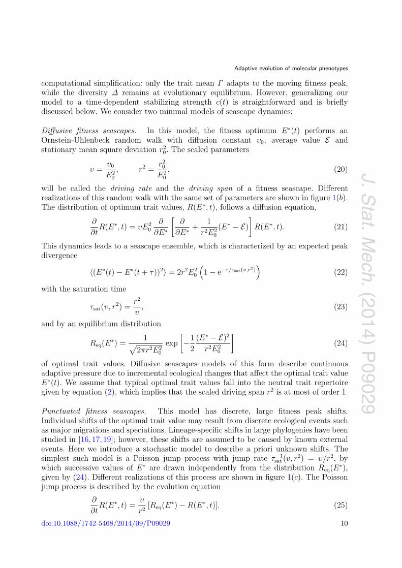
of optimal trait values. Diffusive seascapes models of this form describe continuousadaptive pressure due to incremental ecological changes that affect the optimal trait valueE∗(t). We assume that typical optimal trait values fall into the neutral trait repertoiregiven by equation (2), which implies that the scaled driving span r2 is at most of order 1.

Punctuated fitness seascapes. This model has discrete, large fitness peak shifts.Individual shifts of the optimal trait value may result from discrete ecological events suchas major migrations and speciations. Lineage-specific shifts in large phylogenies have beenstudied in [16, 17, 19]; however, these shifts are assumed to be caused by known externalevents. Here we introduce a stochastic model to describe a priori unknown shifts. Thesimplest such model is a Poisson jump process with jump rate τ−1

sat (v, r2) = υ/r2, bywhich successive values of E∗ are drawn independently from the distribution Req(E∗),given by (24). Different realizations of this process are shown in figure 1(c). The Poissonjump process is described by the evolution equation

∂

∂tR(E∗, t) =

υ

r2 [Req(E∗) − R(E∗, t)]. (25)

doi:10.1088/1742-5468/2014/09/P09029 10

J. Stat. M

ech. (2014) P09029

Adaptive evolution of molecular phenotypes

It has the same time-dependent expected peak divergence (22) and the same equilibriumdistribution (24) as the diffusion process (21) with same driving parameters (20). Thedifference between the jump process and the diffusion process lies in the anomalous scalingof higher moments,

〈(E∗(t) − E∗(t + τ))k〉 ∼ Ek0 rk−2υτ for k = 2, 4, . . . and τ � τsat(υ, r2). (26)

This scaling is shared by simple models of turbulence; see, e.g. [38].

In both types of fitness seascape, we distinguish two dynamical selection regimes:

• Macro-evolutionary fitness seascapes are defined by the condition τsat(v, r2) � τeq(c).As discussed in detail below, such seascapes keep the trait mean always close toequilibrium and induce an adaptive response linear in the driving rate υ. The limitυ → 0 describes an ensemble of quenched population-specific fitness landscapes with adistribution of optimal trait values given by equation (24); see figure 1(d).

• Micro-evolutionary fitness seascapes have τsat(v, r2) � τeq(c) and delineate a regime ofreduced adaptive response, where the evolution of the trait mean gradually decouplesfrom that of the fitness seascape. In the asymptotic fast-driving regime (υ r2/τeq(c)),the adaptation of the trait is completely suppressed. In this regime, we can averageover the fitness fluctuations and describe the macro-evolution of the trait in terms ofan effective fitness landscape with an optimal trait value E .

2.3. Joint dynamics of trait and selection

We now combine the diffusive dynamics of quantitative traits in a given fitness seascape,which is given by equations (7) and (8), and the seascape dynamics (21) or (25) into astochastic model of adaptive evolution. The statistical ensemble generated by this model isillustrated in figures 1(b)–(d): Each population evolves in a specific realization of the fitnessseascape, which is given by a history of peak values E∗(t). Its trait mean Γ (t) follows themoving fitness peak with fluctuations due to mutations and genetic drift. The ensembleof populations contains, in addition, the stochastic differences between realizations of thefitness seascape. The statistics of this ensemble involves combined averages over bothkinds of fluctuations, which are denoted by angular brackets 〈...〉.

The population ensemble can be described by a joint distribution of mean and optimumtrait values, Q(Γ , E∗, t) = Q(Γ , t | E∗)R(E∗, t). Using equations (7) and (21) together withthe projection of the fitness seascape,

F1(Γ | E∗) = f ∗ − c

NE20〈Δ〉 − c

E20(Γ − E∗)2, (27)

given by equations (9) and (17), we obtain the evolution equation for the joint distributionin a diffusive seascape,

∂

∂tQ(Γ , E∗, t) =

[gΓΓ

2N∂2

∂Γ 2 − ∂

∂Γ

(mΓ − gΓΓ 2c

E20(Γ − E∗)

)

+υ

E20

∂2

∂E∗2 +υ

r2

∂

∂E∗ (E∗ − E)]

Q(Γ , E∗, t), (28)

doi:10.1088/1742-5468/2014/09/P09029 11

J. Stat. M

ech. (2014) P09029

Adaptive evolution of molecular phenotypes

with gΓΓ = 〈Δ〉 and mΓ = −2μ(Γ − Γ0). Note that the differential operator inequation (28) is asymmetric: the trait optimum E∗ follows an independent stochasticdynamics, but the trait mean Γ is coupled to E∗. This asymmetry reflects the causalrelation between selection and adaptive response: the trait mean Γ (t) follows themoving fitness peak, as shown in figures 1(b) and (c). As a consequence, the jointevolution equation (28) leads to a non-equilibrium stationary distribution Qstat(Γ , E∗),although the marginal seascape dynamics (21) reaches an equilibrium state. In thefitness landscape limit (υ → 0), the evolution of the trait mean reaches evolutionaryequilibrium; in the opposite limit (υ → ∞), this dynamics can be described byan effective equilibrium. In section 3.1, we will obtain explicit solutions for thenon-equilibrium distribution Qstat(Γ , E∗) and its equilibrium limits. Time-dependentconditional probabilities (propagators) in the stationary ensemble will be discussed insection 3.2 and in appendix A. The case of a punctuated fitness seascape is also treatedin appendix A, where we solve the Langevin equations for Γ and E∗ to obtain the firstand second moments of Q(Γ , E∗, t).

The trait diversity evolves under the projected fitness function

F2(Δ | c) = − c

NE20

Δ, (29)

given by equations (17) and (10). In a fitness seascapes with a constant stabilizing strengthc, this function is time-independent. The dynamics of the trait diversity (8) decouples fromthe adaptive evolution of the trait mean and leads an evolutionary equilibrium Qeq(Δ | c) ofthe form (16). As detailed in section 3.3, the equilibrium assumption for the trait diversityholds for most adaptive processes in a fitness seascape of the form (17). However, we cangeneralize our seascape models to include a time-dependent stabilizing strength c(t). Thisleads to generic adaptive evolution of both, Γ and Δ, which is described by a couplednon-equilibrium stationary distribution Qstat(Γ ,Δ, E∗, c).

2.4. Discussion

We describe the evolution of a quantitative traits by diffusion equations for its populationmean Γ and diversity Δ; see equations (7) and (8). This formalism, which has beenderived in detail in [1], integrates many molecular details into few effective parameters.It provides an analytically tractable and numerically accurate evolutionary description ofmany complex quantitative traits. The dynamics of trait mean and diversity are coupled.For example, the diffusion of Γ depends on the average of Δ, which gives rise to a quasi-neutral evolutionary regime discussed in the next section.

Figure 1 illustrates our model of natural selection: fitness seascapes that have a peakmoving in trait space on macro-evolutionary time scales. The peak displacement followsa stochastic process that models broad classes of evolutionary change. Diffusive seascapesdescribe continuous changes in the optimal trait value, which are ubiquitously generatedby ecological fluctuations. Punctuated seascapes capture large-scale changes caused bydiscrete events, such as speciations or neo-functionalization of genes [39]. Of course, suchmodels are highly idealized representations of biological reality. Their strength lies intheir simplicity: minimal seascapes have just two important evolutionary parameters, thestabilizing strength c and the driving rate υ, which are defined in equations (18) and

doi:10.1088/1742-5468/2014/09/P09029 12

J. Stat. M

ech. (2014) P09029

Adaptive evolution of molecular phenotypes

(20). These parameters can be inferred from data, as we show below in section 5. If thisinference results in useful, testable information about real systems, the underlying modelscan be justified a posteriori.

In a diffusive fitness seascape, the diffusion equation (28) describes the joint dynamicsof mean and optimal trait. However, the role of its two variables are asymmetric: themean trait follows the fitness peak, but the fitness peak moves in an autonomous way.This asymmetry leads to a non-equilibrium evolutionary dynamics, as discussed in thenext section.

3. Adaptive evolution in a single-peak fitness seascape

In this section, we develop the key analytical results of this paper. We provide an explicitsolution for the non-equilibrium joint distribution of mean and optimal trait in a diffusiveseascape, Qstat(Γ , E∗); the case of punctuated seascapes is treated in appendix A. Thesesolutions describe a stationary ensembles of adapting populations. We derive an expressionfor the expected time-dependent trait divergence in these ensembles, which holds for bothseascape models. Finally, we juxtapose the adaptive behavior of the trait mean with theequilibrium statistics of the trait diversity, which emerges in good approximation for mostfitness seascape of constant stabilizing strength. Our analytical results are supported bysimulations for diffusive and punctuated fitness seascapes.

3.1. Stationary distribution of mean and optimal trait

In a diffusive fitness seascape, the evolution equation (28) has a stationary solution ofbivariate Gaussian form,

Qstat(Γ , E∗) =1Z

exp

[−1

2

(ΓE∗

)T

Σ−1(

ΓE∗

)], (30)

where Γ ≡ Γ − 〈Γ 〉 and E∗ ≡ E∗ − E . This distribution is specified by its expectationvalues ( 〈Γ 〉

〈E∗〉)

≡∫

dΓdE∗(

ΓE∗

)Qstat(Γ , E∗)

=(

w(c) E + (1 − w(c))Γ0

E)

, (31)

and the covariance matrix

Σ =( 〈Γ 2〉 〈Γ E∗〉

〈Γ E∗〉 〈E∗2〉)

≡∫

dΓdE∗(

Γ 2 Γ E∗

Γ E∗ E∗2

)Qstat(Γ , E∗)

= E20

((1/2c) w(c) + r2w(c)w(c, υ, r2) r2w(c, υ, r2)

r2w(c, υ, r2) r2

). (32)

doi:10.1088/1742-5468/2014/09/P09029 13

J. Stat. M

ech. (2014) P09029

Adaptive evolution of molecular phenotypes

The distribution Qstat(Γ , E∗) depends on the parameters that characterize the fitnessseascape: the stabilizing strength c, the driving rate υ, and the relative driving span r2,which are defined in equations (18) and (20). Together with the effective population sizeN and the point mutation rate μ, these parameters determine the characteristic timescales of evolution in a fitness seascape, the equilibration time τeq(c) and the saturationtime of fitness fluctuations, τsat(υ, r2); see equations (19) and (23). The function

w(c, υ, r2) ≡ c〈δ〉c〈δ〉 + 2θ + Nυ/r2 =

τ−1eq (c) − μ

τ−1eq (c) − μ + τ−1

sat (υ, r2), (33)

and its equilibrium limit w(c) ≡ w(c, υ=0, r2) govern the coupling between the mean andoptimal trait. The mutation rate μ is the inverse of the neutral timescale τeq(0) = μ−1.These functions depend on the scaled diversity 〈δ〉 ≡ 〈Δ〉/E2

0 , which is given in [1],equations (68)–(73), and is restated below in equation (53). For traits under substantialselection (c � 1), we can distinguish two dynamical regimes: In macro-evolutionaryfitness seascapes, where τsat(υ, r2) � τeq(c) ≈ 2N/(〈δ〉c), this coupling remains closeto the equilibrium value w(c) ≈ 1; micro-evolutionary fitness fluctuations, which haveτsat(υ, r2) � τeq(c), induce a partial decoupling of mean and optimal trait.

We can also express this crossover in terms of the average square distance betweentrait mean in the population and optimal trait of the underlying fitness seascape,

〈Λ2〉 ≡∫

dΓdE∗ (Γ − E∗)2 Qstat(Γ , E∗). (34)

The analytical solution for the scaled quantity 〈λ2〉 ≡ 〈Λ2〉/E20 follows from equations (31)

and (32),

〈λ2〉(c, υ, r2) �

⎧⎪⎪⎪⎨⎪⎪⎪⎩

〈λ2〉eq(c, r2) + υτeq(c)w(c)

2

[1 + O

(τeq

τsat

)], (macroev. seascapes)

〈λ〉eq(c, 0) + r2[1 − O

(τsat

τeq

)], (microev. seascapes),

(35)

where

〈λ2〉eq(c, r2) =w(c)2c

+ (〈λ2〉0 + r2)(1 − w(c))2

� 12c

for c 1 (36)

is the equilibrium average in a fitness landscape. The non-equilibrium contribution reflectsthe lag between the population and the moving fitness peak. In macro-evolutionaryseascapes, this term remains small, which indicates that the trait distribution W(E)closely follows the displacements of the fitness peak. In micro-evolutionary seascapes,the mean square distance 〈λ2〉 becomes comparable to the driving span r2; that is, thepopulation no longer adapts to the moving fitness peak in an efficient way.

doi:10.1088/1742-5468/2014/09/P09029 14

J. Stat. M

ech. (2014) P09029

Adaptive evolution of molecular phenotypes

The distribution Qstat(Γ , E∗) describes a stationary state that is manifestly out ofequilibrium, i.e. it does not have detailed balance. Its probability current

Jstat(Γ , E∗) = −

⎛⎜⎜⎝

gΓΓ

2N∂

∂Γ− mΓ + gΓΓ 2c

NE20(Γ − E∗)

υE20

∂

∂E∗ +υ

r2 (E∗ − E)

⎞⎟⎟⎠Qstat(Γ , E∗)

�

⎧⎪⎪⎪⎪⎪⎪⎪⎨⎪⎪⎪⎪⎪⎪⎪⎩

[−2υc

(Γ − E∗(1 + 1/(2cr2))

(Γ − E∗)

)(1 + O

(τeq

τsat

))]Qstat(Γ , E∗)

(macroev. seascapes),[c〈δ〉N

(E∗

−2cr2Γ

)(1 − O

(τsat

τeq

))]Qstat(Γ , E∗)

(microev. seascapes),(37)

expresses the adaptive motion of the trait mean following the displacements of the fitnesspeak. The probability current shows a crossover similar to the adaptive part of 〈Λ2〉in (35): it increases linearly for low driving rates and saturates to a constant in the regimeof micro-evolutionary fitness fluctuations.

Remarkably, the joint statistics of mean and optimal trait can be associated withevolutionary equilibrium in the limits of low and high driving rates. In the first case, weobtain the equilibrium distribution

Qeq(Γ , E∗) = limυ→0

Qstat(Γ , E∗)

= Q0(Γ ) exp[2NF1(Γ |E∗)] R(E∗)

=1

ZΓ

√2πr2E2

0

exp[− 2θ

〈Δ〉(Γ − Γ0)2 − c

E20(Γ − E∗)2 − 1

2r2E20(E∗ − E)2

],

(38)

which is the product of a Boltzmann distribution (15) and a quenched weight of thetrait optimum E∗ given by (24). This distribution satisfies detailed balance; that is, theprobability current Jstat(Γ , E∗) vanishes in the limit υ → 0. In the opposite limit, weobtain the distribution

Q∞(Γ , E∗) = limυ→∞

Qstat(Γ , E∗)

= Q0(Γ ) exp[2NF1(Γ |E)] R(E∗)

=1

ZΓ

√2πr2E2

0

exp[− 2θ

〈Δ〉(Γ − Γ0)2 − c

E20(Γ − E)2 − 1

2r2E20(E∗ − E)2

].

(39)

In this limit, the fast fluctuations of the fitness peak—and the associated currentJstat(Γ , E∗) given by (37)—decouple from the macro-evolutionary dynamics of the meantrait. The latter is governed by the effective fitness landscape

F1(Γ |E) =∫

F1(Γ |E∗) R(E∗) dE∗, (40)

doi:10.1088/1742-5468/2014/09/P09029 15

J. Stat. M

ech. (2014) P09029

Adaptive evolution of molecular phenotypes

(a) (b) (c)

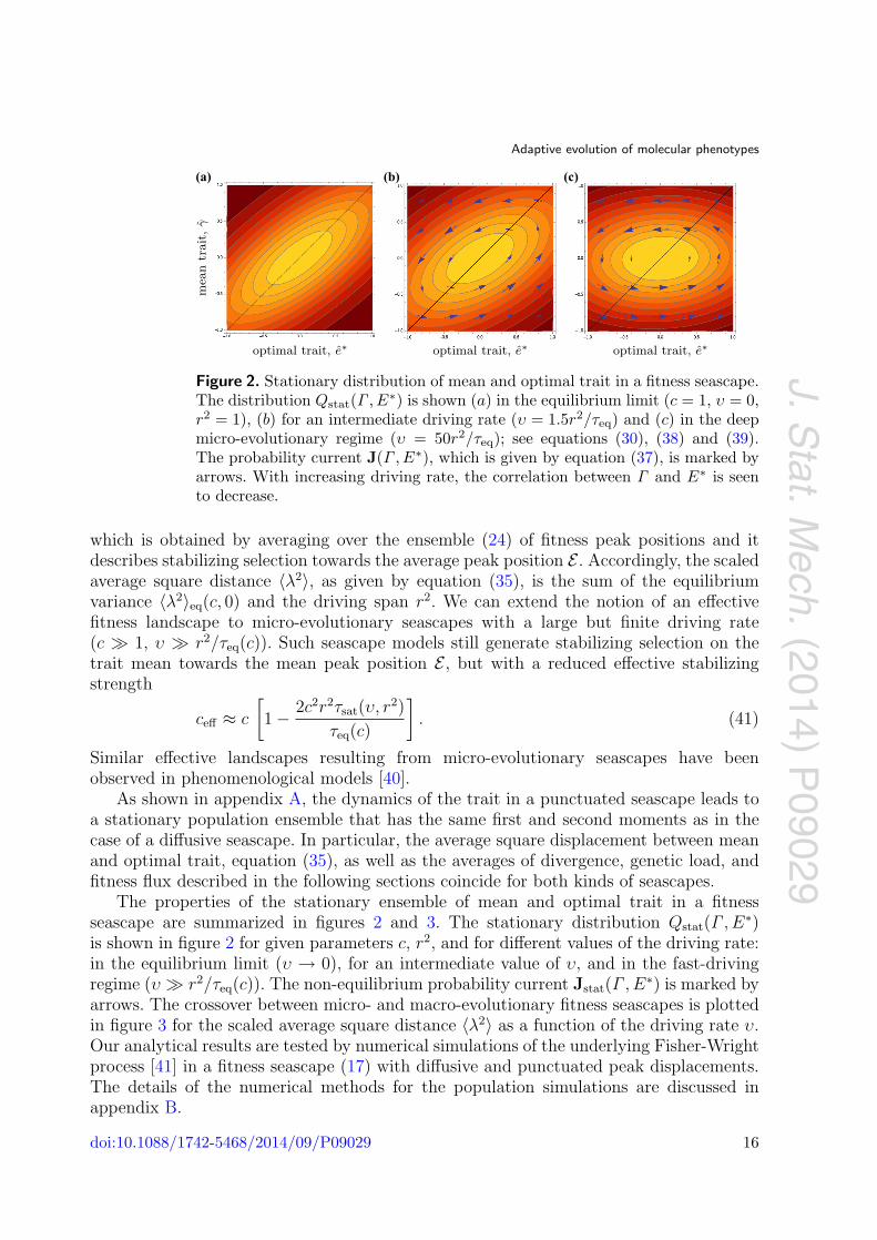
Figure 2. Stationary distribution of mean and optimal trait in a fitness seascape.The distribution Qstat(Γ , E∗) is shown (a) in the equilibrium limit (c = 1, υ = 0,r2 = 1), (b) for an intermediate driving rate (υ = 1.5r2/τeq) and (c) in the deepmicro-evolutionary regime (υ = 50r2/τeq); see equations (30), (38) and (39).The probability current J(Γ , E∗), which is given by equation (37), is marked byarrows. With increasing driving rate, the correlation between Γ and E∗ is seento decrease.

which is obtained by averaging over the ensemble (24) of fitness peak positions and itdescribes stabilizing selection towards the average peak position E . Accordingly, the scaledaverage square distance 〈λ2〉, as given by equation (35), is the sum of the equilibriumvariance 〈λ2〉eq(c, 0) and the driving span r2. We can extend the notion of an effectivefitness landscape to micro-evolutionary seascapes with a large but finite driving rate(c 1, υ r2/τeq(c)). Such seascape models still generate stabilizing selection on thetrait mean towards the mean peak position E , but with a reduced effective stabilizingstrength

ceff ≈ c

[1 − 2c2r2τsat(υ, r2)

τeq(c)

]. (41)

Similar effective landscapes resulting from micro-evolutionary seascapes have beenobserved in phenomenological models [40].

As shown in appendix A, the dynamics of the trait in a punctuated seascape leads toa stationary population ensemble that has the same first and second moments as in thecase of a diffusive seascape. In particular, the average square displacement between meanand optimal trait, equation (35), as well as the averages of divergence, genetic load, andfitness flux described in the following sections coincide for both kinds of seascapes.

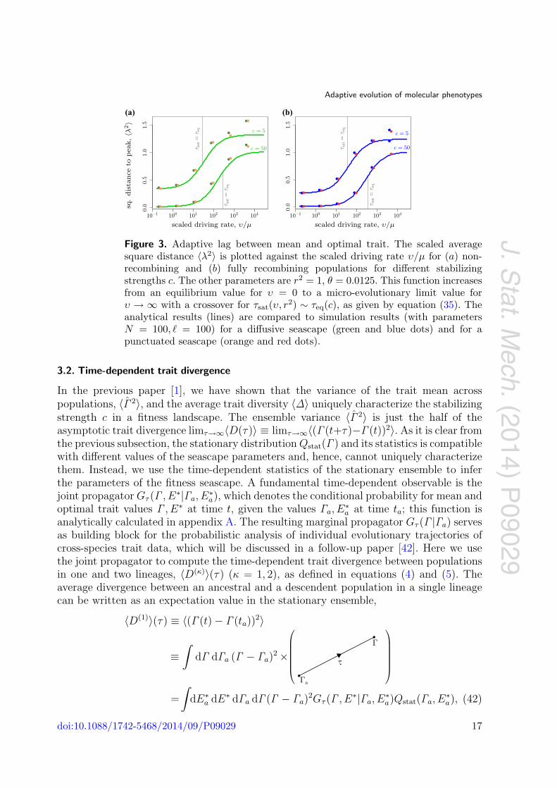
The properties of the stationary ensemble of mean and optimal trait in a fitnessseascape are summarized in figures 2 and 3. The stationary distribution Qstat(Γ , E∗)is shown in figure 2 for given parameters c, r2, and for different values of the driving rate:in the equilibrium limit (υ → 0), for an intermediate value of υ, and in the fast-drivingregime (υ r2/τeq(c)). The non-equilibrium probability current Jstat(Γ , E∗) is marked byarrows. The crossover between micro- and macro-evolutionary fitness seascapes is plottedin figure 3 for the scaled average square distance 〈λ2〉 as a function of the driving rate υ.Our analytical results are tested by numerical simulations of the underlying Fisher-Wrightprocess [41] in a fitness seascape (17) with diffusive and punctuated peak displacements.The details of the numerical methods for the population simulations are discussed inappendix B.

doi:10.1088/1742-5468/2014/09/P09029 16

J. Stat. M

ech. (2014) P09029

Adaptive evolution of molecular phenotypes

(a) (b)

Figure 3. Adaptive lag between mean and optimal trait. The scaled averagesquare distance 〈λ2〉 is plotted against the scaled driving rate υ/μ for (a) non-recombining and (b) fully recombining populations for different stabilizingstrengths c. The other parameters are r2 = 1, θ = 0.0125. This function increasesfrom an equilibrium value for υ = 0 to a micro-evolutionary limit value forυ → ∞ with a crossover for τsat(υ, r2) ∼ τeq(c), as given by equation (35). Theanalytical results (lines) are compared to simulation results (with parametersN = 100, � = 100) for a diffusive seascape (green and blue dots) and for apunctuated seascape (orange and red dots).

3.2. Time-dependent trait divergence

In the previous paper [1], we have shown that the variance of the trait mean acrosspopulations, 〈Γ 2〉, and the average trait diversity 〈Δ〉 uniquely characterize the stabilizingstrength c in a fitness landscape. The ensemble variance 〈Γ 2〉 is just the half of theasymptotic trait divergence limτ→∞〈D(τ)〉 ≡ limτ→∞〈(Γ (t+τ)−Γ (t))2〉. As it is clear fromthe previous subsection, the stationary distribution Qstat(Γ ) and its statistics is compatiblewith different values of the seascape parameters and, hence, cannot uniquely characterizethem. Instead, we use the time-dependent statistics of the stationary ensemble to inferthe parameters of the fitness seascape. A fundamental time-dependent observable is thejoint propagator Gτ (Γ , E∗|Γa, E∗

a), which denotes the conditional probability for mean andoptimal trait values Γ , E∗ at time t, given the values Γa, E∗

a at time ta; this function isanalytically calculated in appendix A. The resulting marginal propagator Gτ (Γ |Γa) servesas building block for the probabilistic analysis of individual evolutionary trajectories ofcross-species trait data, which will be discussed in a follow-up paper [42]. Here we usethe joint propagator to compute the time-dependent trait divergence between populationsin one and two lineages, 〈D(κ)〉(τ) (κ = 1, 2), as defined in equations (4) and (5). Theaverage divergence between an ancestral and a descendent population in a single lineagecan be written as an expectation value in the stationary ensemble,

〈D(1)〉(τ) ≡ 〈(Γ (t) − Γ (ta))2〉

≡∫

dΓ dΓa (Γ − Γa)2 ×

=∫

dE∗a dE∗ dΓa dΓ (Γ − Γa)2Gτ (Γ , E∗|Γa, E∗

a)Qstat(Γa, E∗a), (42)

doi:10.1088/1742-5468/2014/09/P09029 17

J. Stat. M

ech. (2014) P09029

Adaptive evolution of molecular phenotypes

where Γa ≡ Γ (ta), Γ ≡ Γ (t), E∗a ≡ E∗(ta), E∗ ≡ E∗(t), and τ = t − ta. In a similar

way, the average divergence between two descendent populations evolved from a commonancestor population is given by

〈D(2)〉(τ) ≡ 〈(Γ1(t) − Γ2(t))2〉Γ1(ta)=Γ2(ta)E∗

1 (ta)=E∗2 (ta)

≡∫

dΓa dΓ1 dΓ2 (Γ1 − Γ2)2 ×

=∫

dE∗a dE∗

1 dE∗2 dΓa dΓ1 dΓ2 (Γ1 − Γ2)2 Gτ/2(Γ1, E∗

1 |Γa, E∗a)

× Gτ/2(Γ2, E∗2 |Γa, E∗

a) Qstat(Γa, E∗a), (43)

where Γa ≡ Γ1(ta) = Γ2(ta), E∗a ≡ E∗

1(ta) = E∗2(ta), Γi ≡ Γi(t), E∗

i ≡ E∗i (t) (i = 1, 2), and

τ ≡ 2(t − ta). The resulting scaled divergences 〈d(κ)〉(τ) ≡ 〈D(κ)〉(τ)/E20 (κ = 1, 2) can be

calculated using the results of appendix A. We obtain

〈d(κ)〉(τ ; c, υ, r2) =τeq(c)τ(c)

[1 − e−τ/τeq(c)]+ υ w(c, υ, r2)w(c, −υ, r2)

×[τsat(v, r2)(1 − e−τ/τsat(v,r2)) − τeq(c)

(1 − e−τ/τeq(c))]

−2(κ − 1)υ

τ−1eq (c) + τ−1

sat (v, r2)w(c, −υ, r2)2

×[e−τ/(2τsat(v,r2)) − e−τ/(2τeq(c))

]2, (44)

where the equilibration time τeq(c), the saturation time τsat(v, r2), and the coupling factorw(c, υ, r2) are given by equations (19), (23) and (33). The difference between the twodivergence measures is a consequence of the non-equilibrium adaptive dynamics, whichviolate detailed balance. Equation (44) is valid for diffusive and for punctuated fitnessseascapes. It contains the three characteristic time scales defined in the previous section:the drift time τ(c) is the scale over which the diffusion of the trait mean, in the absenceof any fitness seascape, generates a trait divergence of the order of the neutral traitspan E2

0 ; the equilibration time τeq(c) governs the relaxation of the population ensembleto a mutation-selection-drift equilibrium in a fitness landscape of stabilizing strength c;the saturation time τsat(v, r2) is defined by the mean square displacement of the fitnesspeak reaching the driving span r2. Here, we focus on fitness seascapes with substantialstabilizing strength and with a driving span of order of the neutral trait span (c � 1, r2 ∼1). This selection scenario is biologically relevant: it describes adaptive processes that buildup large trait differences by continuous diffusion or recurrent jumps of the fitness peak.

In macro-evolutionary seascapes, the equilibration time and the non-equilibriumsaturation time are well-separated, τeq(c) � τsat(υ, r2). This results in three temporalregimes of the trait divergence:

• Quasi-neutral regime, τ � τeq(c). The scaled divergence takes the form

〈d(κ)〉(τ) = 2〈γ2〉eq(1 − e−τ/τeq

)(45)

� 〈δ〉N

τ (1 + O(τ/τeq)) (κ = 1, 2) (46)

doi:10.1088/1742-5468/2014/09/P09029 18

J. Stat. M

ech. (2014) P09029

Adaptive evolution of molecular phenotypes

with τeq(c) given by equation (19). Its linear initial increase is caused by phenotypicdiffusion with the quasi-neutral diffusion constant Δ/(2N), as given by equations (7)and (12). This diffusion, in turn, is generated by genetic drift and mutations at thetrait loci, which evolve under linkage disequilibrium imposed by stabilizing selectionon the trait diversity Δ, as discussed in [1] and section 3.3. The quasi-neutral increaseof the divergence is bounded by stabilizing selection acting directly on the trait mean;this force becomes important for divergence times of order τeq(c). In the absence ofdirectional selection, it generates a constrained equilibrium divergence

2〈γ2〉eq(c) =w(c)

c. (47)

The quasi-neutral regime (46) should be compared with genuinely neutral traitevolution,

〈d(κ)〉0(τ) =〈δ〉0

μN

(1 − e−μτ

), (48)

which follows from equation (46) in the limit c = 0. The neutral asymptotic behaviorfor short divergence times reduces to a well-known result of classical quantitativegenetics [43–45], 〈D(κ)〉0 = 2Vm(τ/2) with Vm = 〈Δ〉0/N ≈ 4μE2

0 . The saturation fordivergence times of order 1/μ follows the saturation of the genetic divergence at the �constitutive loci.

• Adaptive regime, τeq(c) � τ � τsat(v, r2). The scaled trait divergence follows

〈d(κ)〉(τ) =[2〈γ2〉eq

(1−υ τ κ w(c)2)+ υ w(c)2 τ

][1+O

(e−τ/τeq , τ/τsat

)]� [2〈γ2〉eq + υ (τ − κτeq(c))

]× [1 + O

((θc)2, e−τ/τeq , τ/τsat

)](κ = 1, 2) (49)

In this regime, the trait divergence is the sum of an (asymptotically constant)equilibrium component and an adaptive component, which increases with slope υ.In a macro-evolutionary fitness seascape, this slope is, by definition, smaller thanthe slope in the initial quasi-neutral (46), which allows for a clear delineation of thetwo regimes in empirical data. This feature will be exploited in our selection test forquantitative traits, which will be discussed in section 5.

• Saturation regime, τ � τsat(v, r2). On the largest time scales, the divergence

〈d(κ)〉(τ) ≈ 2〈γ2〉eq + 2r2w(c)w(c, υ, r2)(1 − e−τ/τsat) (κ = 1, 2) (50)

approaches its non-equilibrium saturation value

〈γ2〉stat(c, υ, r2) = 2〈γ2〉eq + 2r2w(c)w(c, υ, r2), (51)

doi:10.1088/1742-5468/2014/09/P09029 19

J. Stat. M

ech. (2014) P09029

Adaptive evolution of molecular phenotypes

which equals the Γ -variance of the stationary distribution Qstat(Γ , E∗), and isprimarily determined by the driving span r2. In empirical data, this regime is oftenwell beyond the depth of the phylogeny and, hence, not observable.

In micro-evolutionary seascapes, the saturation of fitness fluctuations occurs fasterthan the equilibration of the trait under stabilizing selection, i.e. τsat(υ, r2) � τeq(c).Hence, there is a direct crossover from the quasi-neutral to the saturation regime. Forfast micro-evolutionary fitness fluctuations, τsat(υ, r2) � τeq(c), the constraint on thetrait equals that in an effective fitness landscape with stabilizing strength ceff given byequation (41). In this regime, time-dependent trait divergence data alone can no longerresolve adaptive evolution in a fitness seascape from equilibrium in the correspondingeffective fitness landscape; this requires additional information on the trait diversity.

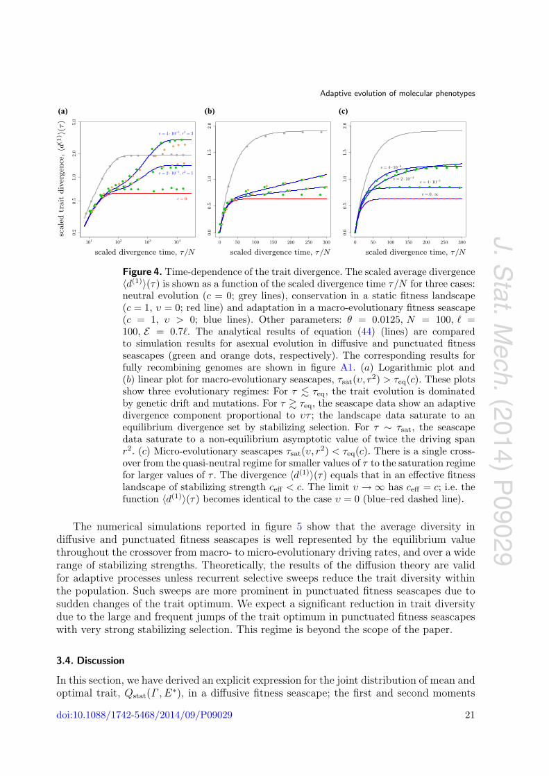
Figures 4 and A1(a) show the scaled divergence 〈d(1)〉(τ) for selection parameters c andυ covering macro-evolutionary and micro-evolutionary fitness seascapes. The analyticalexpression of equation (44) is seen to be in good agreement with numerical simulationsfor diffusive and punctuated fitness fluctuations.

3.3. Stationary trait diversity

As discussed in section 2, our diffusion theory predicts that the movements of theoptimum trait in a single-peak fitness seascape of the form (17) only affects the evolutionof the trait mean in the population and not the trait diversity. The statistics of thetrait diversity remains similar to the case of evolution under stabilizing selection, whichis characterized by a time-invariant fitness function, F2(Δ) = −c0 Δ. The resultingequilibrium distribution Qeq(Δ) is the product of the neutral mutation-drift equilibriumQ0(Δ), which is given in equations (53) and (55) of [1] and a Boltzmann factor from thescaled fitness landscape, Qeq(Δ) = Q0(Δ) exp[−c0 Δ]. These distributions determine theaverage diversity

〈Δ〉 ≡∫

dΔΔQeq(Δ) (52)

and its neutral counterpart 〈Δ〉0, as well as the scaled expectation values 〈δ〉 ≡ 〈Δ〉/E20

and 〈δ〉0 ≡ 〈Δ〉0/E20 . The selective constraint on the trait diversity enters the diffusion

coefficient of the trait mean in equation (7), which sets the drift time scale τ(c) =(1/2μ)(〈δ〉0/〈δ〉(c)), as given by equation (14). The distributions Q0(Δ) and Qeq(Δ)can be written in closed analytical form; unlike in the case of the trait mean, thesedistributions depend directly on the rate of recombination in the population [1]. We obtainthe scaled neutral expectation value 〈δ〉0 = 4θ(1 − 4θ + O(θ2)), which is independent ofthe recombination rate, and the selective constraint

〈δ〉(c)〈δ〉0

={

1 − 4θc + O((θc)2) for θc � 1,(4θc)−1/2 + O((θc)−1) for θc 1 . (53)

in non-recombining populations. We note that this constraint depends only on theproduct θc; therefore, it remains weak over a wide range of parameters (c � 1/θ), whichincludes strong selection effects on the trait mean [1]. The full crossover function and thecorresponding expressions for fully recombining populations are given in equations (68)–(73) of [1].

doi:10.1088/1742-5468/2014/09/P09029 20

J. Stat. M

ech. (2014) P09029

Adaptive evolution of molecular phenotypes

(a) (b) (c)

Figure 4. Time-dependence of the trait divergence. The scaled average divergence〈d(1)〉(τ) is shown as a function of the scaled divergence time τ/N for three cases:neutral evolution (c = 0; grey lines), conservation in a static fitness landscape(c = 1, υ = 0; red line) and adaptation in a macro-evolutionary fitness seascape(c = 1, υ > 0; blue lines). Other parameters: θ = 0.0125, N = 100, � =100, E = 0.7�. The analytical results of equation (44) (lines) are comparedto simulation results for asexual evolution in diffusive and punctuated fitnessseascapes (green and orange dots, respectively). The corresponding results forfully recombining genomes are shown in figure A1. (a) Logarithmic plot and(b) linear plot for macro-evolutionary seascapes, τsat(υ, r2) > τeq(c). These plotsshow three evolutionary regimes: For τ � τeq, the trait evolution is dominatedby genetic drift and mutations. For τ � τeq, the seascape data show an adaptivedivergence component proportional to υτ ; the landscape data saturate to anequilibrium divergence set by stabilizing selection. For τ ∼ τsat, the seascapedata saturate to a non-equilibrium asymptotic value of twice the driving spanr2. (c) Micro-evolutionary seascapes τsat(υ, r2) < τeq(c). There is a single cross-over from the quasi-neutral regime for smaller values of τ to the saturation regimefor larger values of τ . The divergence 〈d(1)〉(τ) equals that in an effective fitnesslandscape of stabilizing strength ceff < c. The limit υ → ∞ has ceff = c; i.e. thefunction 〈d(1)〉(τ) becomes identical to the case υ = 0 (blue–red dashed line).

The numerical simulations reported in figure 5 show that the average diversity indiffusive and punctuated fitness seascapes is well represented by the equilibrium valuethroughout the crossover from macro- to micro-evolutionary driving rates, and over a widerange of stabilizing strengths. Theoretically, the results of the diffusion theory are validfor adaptive processes unless recurrent selective sweeps reduce the trait diversity withinthe population. Such sweeps are more prominent in punctuated fitness seascapes due tosudden changes of the trait optimum. We expect a significant reduction in trait diversitydue to the large and frequent jumps of the trait optimum in punctuated fitness seascapeswith very strong stabilizing selection. This regime is beyond the scope of the paper.

3.4. Discussion

In this section, we have derived an explicit expression for the joint distribution of mean andoptimal trait, Qstat(Γ , E∗), in a diffusive fitness seascape; the first and second moments

doi:10.1088/1742-5468/2014/09/P09029 21

J. Stat. M

ech. (2014) P09029

Adaptive evolution of molecular phenotypes

(a) (b)

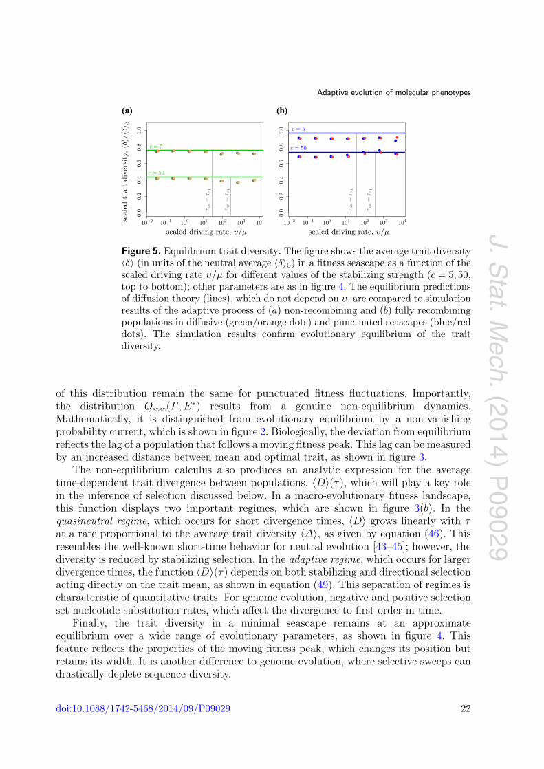
Figure 5. Equilibrium trait diversity. The figure shows the average trait diversity〈δ〉 (in units of the neutral average 〈δ〉0) in a fitness seascape as a function of thescaled driving rate υ/μ for different values of the stabilizing strength (c = 5, 50,top to bottom); other parameters are as in figure 4. The equilibrium predictionsof diffusion theory (lines), which do not depend on υ, are compared to simulationresults of the adaptive process of (a) non-recombining and (b) fully recombiningpopulations in diffusive (green/orange dots) and punctuated seascapes (blue/reddots). The simulation results confirm evolutionary equilibrium of the traitdiversity.

of this distribution remain the same for punctuated fitness fluctuations. Importantly,the distribution Qstat(Γ , E∗) results from a genuine non-equilibrium dynamics.Mathematically, it is distinguished from evolutionary equilibrium by a non-vanishingprobability current, which is shown in figure 2. Biologically, the deviation from equilibriumreflects the lag of a population that follows a moving fitness peak. This lag can be measuredby an increased distance between mean and optimal trait, as shown in figure 3.

The non-equilibrium calculus also produces an analytic expression for the averagetime-dependent trait divergence between populations, 〈D〉(τ), which will play a key rolein the inference of selection discussed below. In a macro-evolutionary fitness landscape,this function displays two important regimes, which are shown in figure 3(b). In thequasineutral regime, which occurs for short divergence times, 〈D〉 grows linearly with τat a rate proportional to the average trait diversity 〈Δ〉, as given by equation (46). Thisresembles the well-known short-time behavior for neutral evolution [43–45]; however, thediversity is reduced by stabilizing selection. In the adaptive regime, which occurs for largerdivergence times, the function 〈D〉(τ) depends on both stabilizing and directional selectionacting directly on the trait mean, as shown in equation (49). This separation of regimes ischaracteristic of quantitative traits. For genome evolution, negative and positive selectionset nucleotide substitution rates, which affect the divergence to first order in time.

Finally, the trait diversity in a minimal seascape remains at an approximateequilibrium over a wide range of evolutionary parameters, as shown in figure 4. Thisfeature reflects the properties of the moving fitness peak, which changes its position butretains its width. It is another difference to genome evolution, where selective sweeps candrastically deplete sequence diversity.

doi:10.1088/1742-5468/2014/09/P09029 22

J. Stat. M

ech. (2014) P09029

Adaptive evolution of molecular phenotypes

4. Fitness and entropy of adaptive processes

The distributions of the trait mean and diversity determine the fitness statistics of anensemble of populations in the stationary state. These statistics can quantify the costand the amount of adaption for the evolution of molecular traits. We also evaluate thepredictability of the trait evolution in an ensemble of populations after diverging from acommon ancestral population.

4.1. Genetic load

The genetic load of an individual population is defined as the difference between themaximum fitness and the mean fitness [46–49],

L(t) ≡ f ∗ − f(t). (54)

For a quantitative trait in a quadratic fitness seascape of the form (17), we can decomposethe load into contributions of the trait mean and diversity,

L(t) = f∗ − c0(Γ (t) − E∗(t))2 − 2c0Δ(t). (55)

In the stationary population ensemble (30), the average scaled genetic load can be writtenas the sum of an equilibrium and an adaptive component,

〈2NL〉(c, υ, r2) = c[〈λ2〉(c, υ, r2) + 〈δ〉(c)]= c[〈λ2〉eq(c, r2) + 〈δ〉(c)] + c[〈λ2〉(c, υ, r2) − 〈λ2〉eq(c, r2)]≡ 2NLeq(c, r2) + 2NLad(c, υ, r2); (56)

these components can be computed analytically from equations (35) and (36). A simpleform is obtained for fitness seascapes of substantial stabilizing strength (c � 1),

2NLeq � 12

+ O(1/c, θc), (57)

2NLad(c, υ, r2) �

⎧⎪⎪⎪⎪⎨⎪⎪⎪⎪⎩

υ τ(c)[1 + O

(τeq

τsat

)], (macroev. seascapes)

cr2[1 − O

(τsat

τeq

)], (microev. seascapes),

(58)

where the drift scale τ(c) is given by equations (14) and (53). From these expressions, weread off three relevant properties of the genetic load.

First, the equilibrium load depends on c only via its diversity component; thisdependence remains weak even for substantial stabilizing selection (1 � c � 1/θ). Theequilibrium load component related to the trait mean, c〈λ2〉eq(c), becomes universal inthis regime: the fluctuations of Γ are constrained to a fitness range of order 2NLeq � 1/2around E∗, irrespectively of the stabilizing strength and the molecular details of the trait[28]. This universality extends to simple nonlinearities in the genotype-phenotype map (1).For a d-component trait as in Fisher’s geometrical model [2], the load formula generalizes

doi:10.1088/1742-5468/2014/09/P09029 23

J. Stat. M

ech. (2014) P09029

Adaptive evolution of molecular phenotypes

(a) (b)

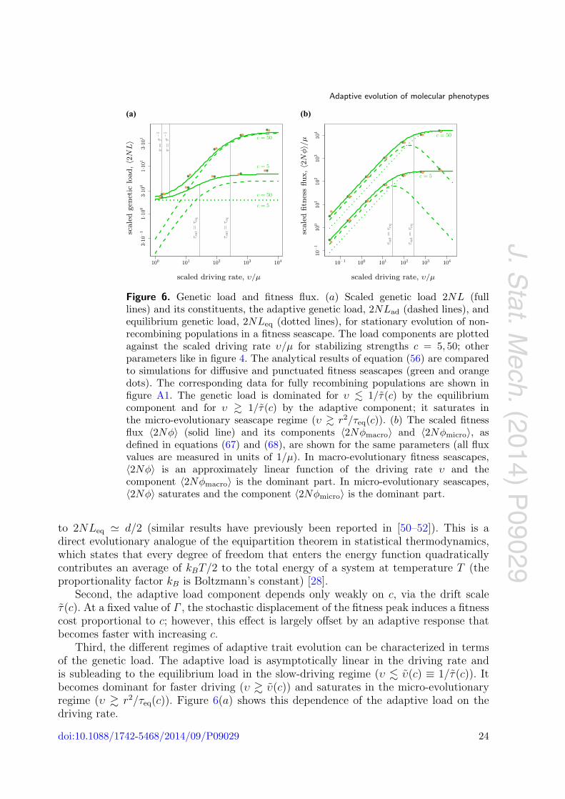
Figure 6. Genetic load and fitness flux. (a) Scaled genetic load 2NL (fulllines) and its constituents, the adaptive genetic load, 2NLad (dashed lines), andequilibrium genetic load, 2NLeq (dotted lines), for stationary evolution of non-recombining populations in a fitness seascape. The load components are plottedagainst the scaled driving rate υ/μ for stabilizing strengths c = 5, 50; otherparameters like in figure 4. The analytical results of equation (56) are comparedto simulations for diffusive and punctuated fitness seascapes (green and orangedots). The corresponding data for fully recombining populations are shown infigure A1. The genetic load is dominated for υ � 1/τ(c) by the equilibriumcomponent and for υ � 1/τ(c) by the adaptive component; it saturates inthe micro-evolutionary seascape regime (υ � r2/τeq(c)). (b) The scaled fitnessflux 〈2Nφ〉 (solid line) and its components 〈2Nφmacro〉 and 〈2Nφmicro〉, asdefined in equations (67) and (68), are shown for the same parameters (all fluxvalues are measured in units of 1/μ). In macro-evolutionary fitness seascapes,〈2Nφ〉 is an approximately linear function of the driving rate υ and thecomponent 〈2Nφmacro〉 is the dominant part. In micro-evolutionary seascapes,〈2Nφ〉 saturates and the component 〈2Nφmicro〉 is the dominant part.

to 2NLeq � d/2 (similar results have previously been reported in [50–52]). This is adirect evolutionary analogue of the equipartition theorem in statistical thermodynamics,which states that every degree of freedom that enters the energy function quadraticallycontributes an average of kBT/2 to the total energy of a system at temperature T (theproportionality factor kB is Boltzmann’s constant) [28].

Second, the adaptive load component depends only weakly on c, via the drift scaleτ(c). At a fixed value of Γ , the stochastic displacement of the fitness peak induces a fitnesscost proportional to c; however, this effect is largely offset by an adaptive response thatbecomes faster with increasing c.

Third, the different regimes of adaptive trait evolution can be characterized in termsof the genetic load. The adaptive load is asymptotically linear in the driving rate andis subleading to the equilibrium load in the slow-driving regime (υ � υ(c) ≡ 1/τ(c)). Itbecomes dominant for faster driving (υ � υ(c)) and saturates in the micro-evolutionaryregime (υ � r2/τeq(c)). Figure 6(a) shows this dependence of the adaptive load on thedriving rate.

doi:10.1088/1742-5468/2014/09/P09029 24

J. Stat. M

ech. (2014) P09029

Adaptive evolution of molecular phenotypes

4.2. Fitness flux

The fitness flux, φ(t), characterizes the adaptive response of a population evolving in afitness land- or seascape,

φ(t) =∫

dE f(E, t)∂

∂tW(E, t). (59)

The cumulative fitness flux, Φ(τ) =∫ t+τ

tφ(t′)dt′, measures the total amount of adaptation

over an evolutionary period τ [53]. The evolutionary statistics of this quantity is specifiedby the fitness flux theorem [20]. According to the theorem, the average cumulativefitness flux in a population ensemble measures the deviation of the evolutionary processfrom equilibrium: this deviation equals the relative entropy of the actual processfrom a hypothetical time-reversed process [20, 54]. It is substantial—i.e. the processis predominantly adaptive—if 〈2NΦ〉 � 1. Specifically, the cumulative fitness flux ofa stationary adaptive process increases linearly with time, 〈2NΦ(τ)〉 = 〈2Nφ〉τ with〈φ〉 > 0.

For a quantitative trait in a quadratic fitness seascape of the form (17), we candecompose the fitness flux into contributions of the trait mean and the trait diversity,

φ(t) = −2c0(Γ (t) − E∗(t))dΓ (t)

dt− 2c0

dΔ(t)dt

. (60)

In the stationary population ensemble (30), the average scaled fitness flux can be expressedin terms of the stationary probability current Jstat(Γ , E∗),

〈2Nφ〉 = − 2cE2

0

∫dΓdE∗ (Γ − E∗)JΓ

stat(Γ , E∗), (61)

where JΓstat(Γ , E∗) is the Γ–component of Jstat(Γ , E∗). The fitness flux can be computed

analytically from equation (37),

〈2Nφ〉(c, υ, r2) = 2cυ w(c, υ, r2). (62)

In the regime of substantial stabilizing strength (c � 1), we get

〈2Nφ〉(c, υ, r2) �

⎧⎪⎪⎪⎪⎨⎪⎪⎪⎪⎩

2cυ[1 − O

(τeq

τsat

)](macroev. seascapes),

4c2r2

τ(c)

[1 − O

(τsat

τeq

)](microev. seascapes),

(63)

where the drift time τ(c) is given by equations (14) and (53). The fitness flux dependslinearly on the driving rate in a macro-evolutionary fitness seascape, and it saturates inthe regime of micro-evolutionary fitness fluctuations. Figure 6(b) shows this dependenceof the fitness flux on the driving rate.

We can express the fitness flux in terms of correlation functions of the trait meanΓ (t) and the lag Λ(t), which results in a simple relation between fitness flux and adaptive

doi:10.1088/1742-5468/2014/09/P09029 25

J. Stat. M

ech. (2014) P09029

Adaptive evolution of molecular phenotypes

load. Inserting the probability current of equation (37) into the integral of equation (61),we find

〈2Nφ〉 =2c2〈δ〉

E20

(〈Λ2〉 − 〈Λ2〉eq)

(64)

+4cθE2

0limτ↘0

(〈Λ(t + τ)(Γ (t) − Γ0)〉 − 〈Λ(t + τ)(Γ (t) − Γ0)〉eq)

= c〈δ〉〈2NL〉ad(c, υ, r2)[1 + O(θ)].

From this representation, we obtain the spectral decomposition of the fitness flux,

〈2Nφ〉(c, υ, r2) =∫ ∞

0〈2Nφ(ω)〉 dω (65)

with

〈2Nφ(ω)〉 = 2cυc〈δ〉π/2

ω2

(τ−2eq (c) + ω2)(τ−2

sat (υ, r2) + ω2)[1 + O(θ/(c〈δ〉)]. (66)

Using a cutoff frequency ωc = k/τeq(c) with a constant k of order 1, we can now define amacro-evolutionary flux component,

〈2Nφmacro〉 =∫ ωc

0〈2Nφ(ω)〉 dω = 2cυ w(c, υ, r2)

×(τ−1eq (c) + 2μ) arctan[k] − (τ−1

sat (υ, r2) + 2μ) arctan [k τsat(v, r2)/τeq(c)](π/2)(τ−1

eq (c) − τ−1sat (υ, r2))

,

(67)

and the complementary micro-evolutionary component

〈2Nφmicro〉 =∫ ∞

ωc

〈2Nφ(ω)〉 dω = 〈2Nφ〉 − 〈2Nφmacro〉. (68)

In the regime of substantial stabilizing selection (c � 1), the macro-evolutionary fitnessflux in (67) reads

〈2Nφmacro〉(c, υ, r2) �

⎧⎪⎪⎪⎨⎪⎪⎪⎩

2cυ2π

arctan[k], (macroev. seascapes)

2cυτ 2sat(υ, r2)τ 2eq(c)

2π

(k − arctan[k]) ∼ 1v, (microev. seascapes)

(69)

This fitness flux component quantifies the macro-evolutionary part of adaptation. Inmacro-evolutionary fitness seascapes (τsat(υ, r2) � τeq(c)), it increases proportionally tothe driving rate υ and, for k > 1, it represents the main fraction of the total fitnessflux 〈2Nφ〉. In micro-evolutionary fitness seascapes (τsat(υ, r2) � τeq(c)), this componentis suppressed: the macro-evolutionary fitness flux does not carry information on rapidfitness fluctuations. This cross-over of 〈2Nφmacro〉 and of the complementary component〈2Nφmicro〉 is shown in figure 6(b).

The spectral decomposition of the fitness flux has important consequences for theanalysis of macro-evolutionary adaptation. The detection of a substantial cumulative

doi:10.1088/1742-5468/2014/09/P09029 26

J. Stat. M

ech. (2014) P09029

Adaptive evolution of molecular phenotypes

fitness flux 〈2NΦmacro(τ)〉 > 1 over a macro-evolutionary period τ is not confounded by thesimultaneous presence of micro-evolutionary (for example seasonal) fitness fluctuations.Since the cumulative fitness flux is a measure of entropy production during adaptation, thespectral decomposition (65) also has an important information-theoretic interpretation:The difference 〈2Nφmicro〉 = 〈2Nφ〉 − 〈2Nφmacro〉 is the average loss of information perunit time through temporal coarse-graining. This loss is a non-equilibrium analogue ofthe entropy production by spatial coarse-graining.

4.3. Predictability and entropy production

In [1], we quantified the evolutionary predictability of the molecular traits across anensemble of populations by

P ≡ exp [〈S(W)〉 − S(〈W 〉)], (70)

with S(W) ≡ − ∫ W(E) log W(E)dE. This definition compares the ensemble-averaged‘micro-evolutionary’ Shannon entropy of the phenotype distribution within a population,〈S(W)〉 ≡ ∫W S(W) Q(W), and the ‘macro-evolutionary’ Shannon entropy of the mixeddistribution, S(〈W〉) ≡ S(

∫W W Q(W)), which is obtained by compounding the trait

values of all populations into a single distribution. We have shown that the predictability isgenerically low in a neutral ensemble, but stabilizing selection in a single fitness landscapecan generate an evolutionary equilibrium with predictability values P of order 1 [1].

Here we compute the predictability in a time-dependent ensemble of populations thatdescend from a common ancestor population. Similarly to [1], we evaluate equation (70) fora distribution Qt(W) with the initial condition Qta(W) = δ(W −Wa) at time ta = t−τ/2.We obtain the time-dependent predictability

P(τ ; c, υ, r2) �( 〈δ〉(c)

〈d(2)〉(τ ; c, υ, r2)/2 + 〈δ〉(c))1/2

=(

11 + Ω (2)(τ ; c, υ, r2)/4θ

)1/2

. (71)

Here, Ω (2)(τ ; c, v, r2) ≡ 2θ 〈d(2)〉(τ ; c, υ, r2)/〈δ〉 denotes the ratio between trait divergenceand diversity for the descendent populations. The trait statistics in a macro-evolutionaryfitness seascape, given by equations (44) and (53), entail the evolutionary predictability

P(τ ; c, υ, r2) = Peq(c)[1 − 1

2υ τ

τ − 2τeq(c)2N

[1 + O (τ τeq(c)cv/N , τ/τsat, θ/(c〈δ〉))

]](72)

for τ � τeq(c), with Peq(c) = (1 + w(c)/(2c))−1/2 = (1 + 1/(2c))−1/2[1 + O(θ/(c〈δ〉))].There are two stochastic components that generate macro-evolutionary entropy and,hence, reduce the evolutionary predictability: fluctuations induced by genetic drift onshort time-scales τ � τeq(c) and fluctuations of the fitness peak over time-scales τ � τeq(c).Nevertheless, as shown by (72), the predictability of an adaptive process with substantialstabilizing selection can remain of order 1 over macro-evolutionary periods.

4.4. Discussion

In this section, we have introduced three simple summary observables of evolutionaryprocesses: genetic load, fitness flux, and predictability. For quantitative traits, the

doi:10.1088/1742-5468/2014/09/P09029 27

J. Stat. M

ech. (2014) P09029

Adaptive evolution of molecular phenotypes

statistics of these observables is universal; that is, it decouples from details of molecularevolution.

Genetic load is defined as the difference between the maximum of a fitness land- orseascape and the mean fitness in a population. Here we have evaluated the load associatedwith a quantitative trait. In evolutionary equilibrium under substantial stabilizingselection, the load takes the simple universal form L = 1/(4N), which generalizes toL = d/(4N) for a d-dimensional quantitative trait in a quadratic fitness landscape (see[50–52] for similar results). This universal strong-selection behavior of the equilibriumload distinguishes quantitative traits from individual genetic loci, for which L ∼ 1/Nsignals weak selection3 (i.e. selection coefficients of order 1/N). In fitness seascapes, thereis an additional nonequilibrium load component, which is proportional to the driving rateυ and measures the fitness cost of adaptation. We still know little on how this type ofload affects real populations. However, studies at the genetic level suggest it may play animportant role in rapid asexual adaptation processes, which occur in microbial or viralpopulations [55,56].

Fitness flux measures the fitness gain through adaptive changes per unit ofevolutionary time; the cumulative fitness flux is the total adaptive fitness gain over anevolutionary period [20]. These universal measures serve to compare adaptive processes indifferent populations. In empirical studies, the fitness flux has been evaluated in systemsas diverse as flies and influenza viruses [53, 55, 57]. Here we have shown that the fitnessflux of a quantitative trait in a fitness seascape is proportional to stabilizing strength anddriving rate, φ ≈ 2cυ.

Predictability has been an important issue in laboratory evolution experiments,which can be repeated multiple times under similar conditions. For a quantitativetrait, predictability can be defined in a straightforward way [1]: How much of the traitrepertoire in an ensemble of parallel-evolving populations is already contained in the traitdiversity of a single population? We have shown that fitness seascapes have antagonisticeffects: stabilizing selection enhances, lineage-specific directional selection decreasespredictability. Adaptive process in macro-evolutionary fitness seascapes can maintainsubstantial predictability values over macro-evolutionary periods. Parallel and convergentevolution at the functional level, paired with strongly divergent genome evolution has beenobserved in a number of recent experiments [58–60]. These experimental observations canbe explained in a natural way, if we assume that many of these functions involve a complexquantitative trait.

5. Inference of adaptive trait evolution

The statistical theory developed in this paper suggests a new method to infer selectionon quantitative traits. Our method is based on trait evolution in a single-peak fitnessseascape, as defined in equation (17), which is parametrized by its stabilizing strength cand its driving rate υ.

3 For a quantitative trait, L ∼ 1/N holds over a broad range of stabilizing strengths [1]. Hence, this estimatecannot be used to infer weak selection, as claimed in [18].

doi:10.1088/1742-5468/2014/09/P09029 28

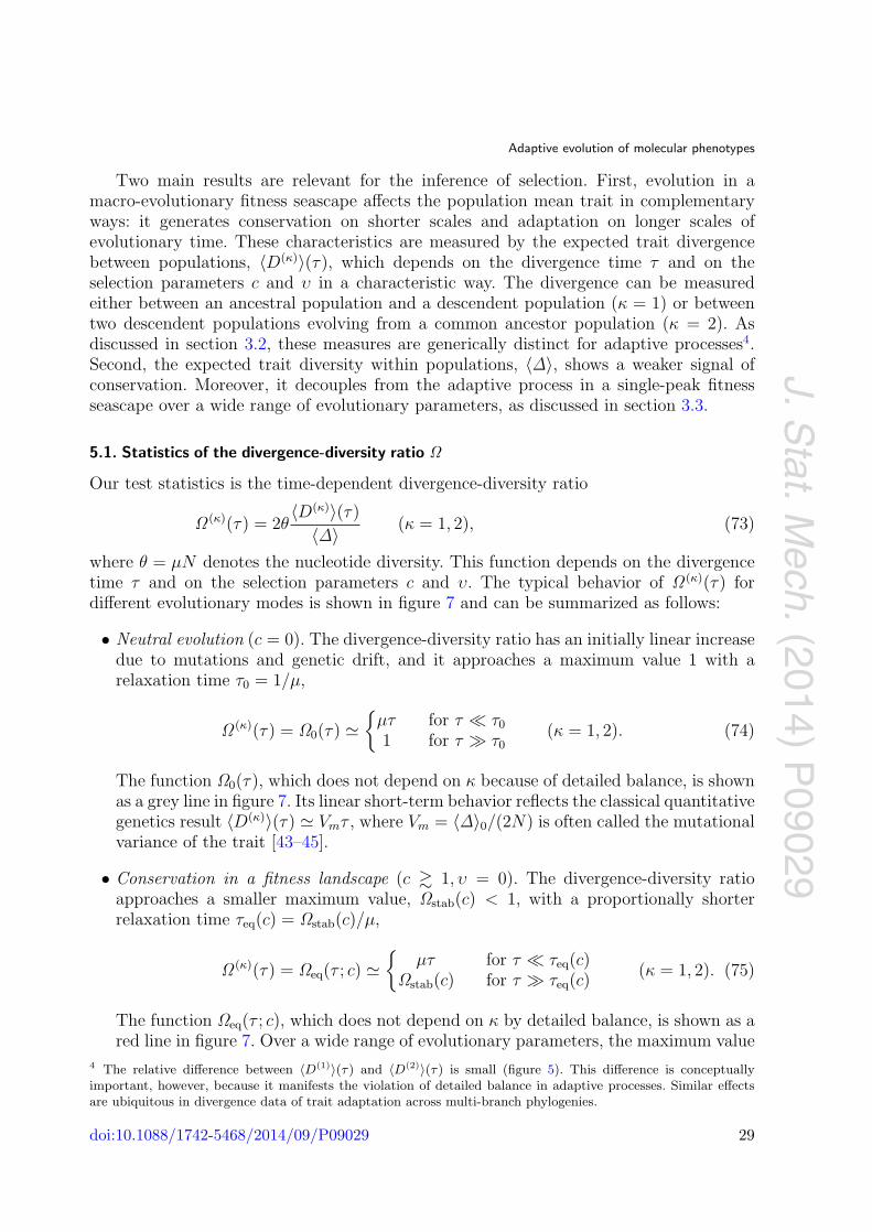
J. Stat. M

ech. (2014) P09029

Adaptive evolution of molecular phenotypes

Two main results are relevant for the inference of selection. First, evolution in amacro-evolutionary fitness seascape affects the population mean trait in complementaryways: it generates conservation on shorter scales and adaptation on longer scales ofevolutionary time. These characteristics are measured by the expected trait divergencebetween populations, 〈D(κ)〉(τ), which depends on the divergence time τ and on theselection parameters c and υ in a characteristic way. The divergence can be measuredeither between an ancestral population and a descendent population (κ = 1) or betweentwo descendent populations evolving from a common ancestor population (κ = 2). Asdiscussed in section 3.2, these measures are generically distinct for adaptive processes4.Second, the expected trait diversity within populations, 〈Δ〉, shows a weaker signal ofconservation. Moreover, it decouples from the adaptive process in a single-peak fitnessseascape over a wide range of evolutionary parameters, as discussed in section 3.3.

5.1. Statistics of the divergence-diversity ratio Ω

Our test statistics is the time-dependent divergence-diversity ratio

Ω (κ)(τ) = 2θ〈D(κ)〉(τ)

〈Δ〉 (κ = 1, 2), (73)

where θ = μN denotes the nucleotide diversity. This function depends on the divergencetime τ and on the selection parameters c and υ. The typical behavior of Ω (κ)(τ) fordifferent evolutionary modes is shown in figure 7 and can be summarized as follows:

• Neutral evolution (c = 0). The divergence-diversity ratio has an initially linear increasedue to mutations and genetic drift, and it approaches a maximum value 1 with arelaxation time τ0 = 1/μ,

Ω (κ)(τ) = Ω0(τ) �{

μτ for τ � τ0

1 for τ τ0(κ = 1, 2). (74)

The function Ω0(τ), which does not depend on κ because of detailed balance, is shownas a grey line in figure 7. Its linear short-term behavior reflects the classical quantitativegenetics result 〈D(κ)〉(τ) � Vmτ , where Vm = 〈Δ〉0/(2N) is often called the mutationalvariance of the trait [43–45].

• Conservation in a fitness landscape (c � 1, υ = 0). The divergence-diversity ratioapproaches a smaller maximum value, Ωstab(c) < 1, with a proportionally shorterrelaxation time τeq(c) = Ωstab(c)/μ,

Ω (κ)(τ) = Ωeq(τ ; c) �{

μτ for τ � τeq(c)Ωstab(c) for τ τeq(c)

(κ = 1, 2). (75)

The function Ωeq(τ ; c), which does not depend on κ by detailed balance, is shown as ared line in figure 7. Over a wide range of evolutionary parameters, the maximum value

4 The relative difference between 〈D(1)〉(τ) and 〈D(2)〉(τ) is small (figure 5). This difference is conceptuallyimportant, however, because it manifests the violation of detailed balance in adaptive processes. Similar effectsare ubiquitous in divergence data of trait adaptation across multi-branch phylogenies.

doi:10.1088/1742-5468/2014/09/P09029 29

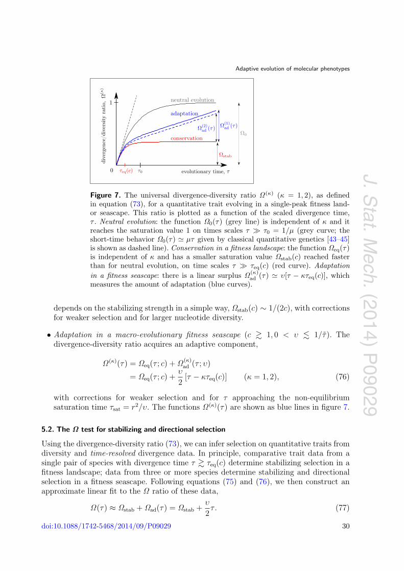
J. Stat. M

ech. (2014) P09029

Adaptive evolution of molecular phenotypes

Figure 7. The universal divergence-diversity ratio Ω (κ) (κ = 1, 2), as definedin equation (73), for a quantitative trait evolving in a single-peak fitness land-or seascape. This ratio is plotted as a function of the scaled divergence time,τ . Neutral evolution: the function Ω0(τ) (grey line) is independent of κ and itreaches the saturation value 1 on times scales τ τ0 = 1/μ (grey curve; theshort-time behavior Ω0(τ) � μτ given by classical quantitative genetics [43–45]is shown as dashed line). Conservation in a fitness landscape: the function Ωeq(τ)is independent of κ and has a smaller saturation value Ωstab(c) reached fasterthan for neutral evolution, on time scales τ τeq(c) (red curve). Adaptationin a fitness seascape: there is a linear surplus Ω (κ)

ad (τ) � υ[τ − κτeq(c)], whichmeasures the amount of adaptation (blue curves).

depends on the stabilizing strength in a simple way, Ωstab(c) ∼ 1/(2c), with correctionsfor weaker selection and for larger nucleotide diversity.

• Adaptation in a macro-evolutionary fitness seascape (c � 1, 0 < υ � 1/τ). Thedivergence-diversity ratio acquires an adaptive component,

Ω (κ)(τ) = Ωeq(τ ; c) + Ω (κ)ad (τ ; υ)

= Ωeq(τ ; c) +υ

2[τ − κτeq(c)] (κ = 1, 2), (76)

with corrections for weaker selection and for τ approaching the non-equilibriumsaturation time τsat = r2/υ. The functions Ω (κ)(τ) are shown as blue lines in figure 7.

5.2. The Ω test for stabilizing and directional selection

Using the divergence-diversity ratio (73), we can infer selection on quantitative traits fromdiversity and time-resolved divergence data. In principle, comparative trait data from asingle pair of species with divergence time τ � τeq(c) determine stabilizing selection in afitness landscape; data from three or more species determine stabilizing and directionalselection in a fitness seascape. Following equations (75) and (76), we then construct anapproximate linear fit to the Ω ratio of these data,

Ω(τ) ≈ Ωstab + Ωad(τ) = Ωstab +υ

2τ . (77)

doi:10.1088/1742-5468/2014/09/P09029 30

J. Stat. M

ech. (2014) P09029

Adaptive evolution of molecular phenotypes

We obtain simple estimates of stabilizing strength and driving rate,

c ≈ 1Ωstab

, υ ≈ 2Ωad(τ)τ

, (78)

and we infer that a fraction

ωad(τ) ≡ Ωad(τ)Ω(τ)

=Ω(τ) − Ωstab

Ω(τ)(79)

of the observed trait divergence is adaptive, i.e. driven by directional selection.The Ω test reflects generic characteristics of quantitative trait evolution, which are

described by equations (74)–(76): The expected trait divergence 〈D〉(τ) always grows ina quasi-neutral linear way for divergence times τ � τeq(c); beyond this regime, it dependson both stabilizing and directional selection. This behavior has important consequencesfor applications. First, the Ω test is insensitive to selection if the species comparedare too close. Second, cross-species comparisons that provide evidence for enhanced Ωvalues in a single lineage cannot distinguish directional from relaxed stabilizing selection.These limitations may partially explain the difficulties to infer system-wide evidence fordirectional selection on gene expression [61–63].

An important prerequisite for the wide applicability of the Ω test is its universality: thedivergence-diversity ratio depends on the selection parameters c and υ, but it decouplesfrom the trait’s genetic basis. In particular, it depends only weakly on the number andtrait amplitudes of the constitutive sequence sites, and on the amount of recombinationbetween these sites. All of these genetic factors are, in general, unknown. They act asconfounding factors for an inference of selection based on non-universal observables [18].The Ω statistics also decouples from details of the selection dynamics; it can be appliedto continual as well as to punctuated adaptive processes. We have tested this universalityby extensive numerical simulations, which are reported in appendix B.

The Ω test is based on ensemble averages of trait divergence and diversity. Ourstatistical theory also specifies the deviations of individual evolutionary trajectories fromthe ensemble averages; these fluctuations are described by the propagator functions inappendix A. We can use the propagator statistics to build a hidden Markov model for theinference of selection from noisy trajectories of individual traits. This method is essentialin the analysis of trait divergence over phylogenies of species, which is described in detailin a follow-up paper [42].

5.3. Comparison with sequence-based inference of selection

The Ω test for selection on quantitative traits is related to a test for adaptive sequenceevolution of the McDonald-Kreitman type [64]. This test evaluates the divergence-diversityratio Ω for a sequence class under putative selection (e.g. nonsynonymous mutations inprotein-coding sequence) and compares it to the analogous ratio Ω0 for bona fide neutralchanges (e.g. synonymous mutations). Positive selection in the query sequence is inferredif Ω > Ω0. In this case, the amplitude ratio

α =Ω − Ω0

Ω(80)

estimates the fraction of nonsynonymous substitutions that are adaptive, i.e. driven bypositive selection [65].

doi:10.1088/1742-5468/2014/09/P09029 31

J. Stat. M

ech. (2014) P09029

Adaptive evolution of molecular phenotypes

Comparing the two inference schemes reveals a number of important differences. Unlikethe McDonald-Kreitman test, the Ω test for quantitative traits does not require a ‘nulltrait’ that evolves near neutrality and takes the role of synonymous sequences. Indeed, nosuch neutral trait gauge is available in most cases. Instead, the Ω test compares data fromthree or more species, while the McDonald-Kreitman test requires only a single pair ofspecies. Moreover, the Ω test includes the inference of the stabilizing strength, while theMcDonald-Kreitman test leaves the strength of selection undetermined (large selectioncoefficients of beneficial alleles are an input assumption for the estimate (80)).

6. Conclusion

In this paper, we have developed a statistical theory for the evolution of a quantitativetrait in a stochastic fitness seascape. The fitness model used for our analysis, a single-peak seascape with diffusive or punctuated peak displacements, covers a broad spectrumof biologically relevant evolutionary scenarios [28]. The two seascape parameters c and υquantify stabilizing and directional selection on the trait, which, in turn, govern the trait’sfundamental evolutionary modes of conservation and adaptation. Our analysis shows thatthese modes are not mutually exclusive, but are joint features of dynamic selection models.

In a macro-evolutionary fitness seascape, conservation and adaptation are associatedwith different time scales: conservation is observed on shorter scales, while adaptivechanges build up on longer scales of evolutionary time. Micro-evolutionary fitnessfluctuations, on the other hand, lead to reduced genetic adaptation, which decouplesfrom the macro-evolutionary dynamics of the trait. Rapid adaptive response to seasonal orother fluctuations of the environment often involves epigenetic modifications or phenotypicswitching [40]. The evolutionary roles of these mechanisms are beyond the scope of thispaper. The spectral decomposition of the fitness flux, which has been introduced above,quantifies how the adaptive process is distributed on different scales of evolutionary time.

Our theory suggests new inference methods for selection on quantitative traits, whichhave important potential applications. At the sequence level, an increasingly complexpicture of selection has emerged in recent years. Notably, we have acquired a growingrepertoire of empirical genotype-fitness landscapes [66], which has generated importantexperimental and theoretical insights into the evolutionary dynamics on these landscapes.However, we still know little about the statistical properties of empirical phenotype-fitnessmaps, and next to nothing about phenotype-dependent seascapes. Systematic inference ofselection on molecular quantitative traits, such as levels of gene expression and enzymaticactivity, can contribute to close this gap. Eventually, fitness land- and seascapes forindividual traits will need to be integrated into larger phenotype-fitness maps, whichinclude fitness interactions between traits.

Appendix A. Analytical theory of the adaptive ensemble

In section 3.1, we obtained the Gaussian stationary distribution Qstat(Γ , E∗) in a diffusiveseascape from the underlying Fokker-Planck equation (7). Here we use a Langevin

doi:10.1088/1742-5468/2014/09/P09029 32

J. Stat. M

ech. (2014) P09029

Adaptive evolution of molecular phenotypes

representation to compute the time-resolved trait divergence 〈d(κ)〉(τ) (κ = 1, 2). Thisderivation, which reproduces mean and variance of the distribution Qstat(Γ , E∗), appliesto diffusive and punctuated fitness seascapes. We also compute the full propagatorfunction Gτ (Γ , E∗|Γa, E∗

a) for macro-evolutionary diffusive seascapes. The propagator ina punctuated fitness seascape has the same mean and variance, but differs in higher traitmoments.

A.1. Moments of the optimal trait

In a diffusive seascape, the fitness peak E∗(t) follows an Ornstein–Uhlenbeck process withLangevin representation

∂tE∗(t) = − υ

r2 (E∗(t) − E) + η(t), (A.1)

where η(t) is a Gaussian random variable with the statistics

〈η(t)〉 = 0, 〈η(t)η(t′)〉 = 2υE20 δ(t − t′). (A.2)

Formally solving equation (A.1),

E∗(t + τ) = E∗(t)e−τ/τsat + E(1 − e−τ/τsat) +∫ t2

t1

dt′ e−(τ−t′)/τsatη(t′), (A.3)

and evaluating the noise correlations (A.2), we obtain the average peak value with aninitial condition E∗(t) = Ea and the autocorrelation function of the fitness peak in thestationary ensemble,

〈E∗(t + τ)〉(Ea) = Eae−τ/τsat + E(1 − e−τ/τsat), (A.4)

〈E∗(t)E∗(t + τ)〉 = E2 + E20r

2e−τ/τsat . (A.5)

It is straightforward to check that equations (A.4) and (A.5) are valid also for punctuatedseascapes.

A.2. Moments of the trait mean

The Langevin equation for Γ (t) reads

∂tΓ (t) = −2μ(Γ (t) − Γ0) − 〈Δ〉 2cE2

0(Γ (t) − E∗(t)) + ξ(t), (A.6)

where ξ(t) is a Gaussian noise with the statistics

〈ξ(t)〉 = 0, 〈ξ(t)ξ(t′)〉 =〈Δ〉N

δ(t − t′), 〈ξ(t)E∗(t′)〉 = 0. (A.7)

For diffusive seascapes, the last term in (A.7) is equivalent to 〈ξ(t)η(t′)〉 = 0, which impliesthat genetic drift and fitness seascape fluctuations are independent. The formal solutionof equation (A.6) reads

Γ (t + τ) = e−τ/τeqΓ (t) + (1−w(c))(1 − e−τ/τeq)Γ0

+∫ t+τ

t

dt′ (E∗(t′)c〈δ〉 + ξ(t′)) e−(t+τ−t′)/τeq , (A.8)

doi:10.1088/1742-5468/2014/09/P09029 33

J. Stat. M

ech. (2014) P09029

Adaptive evolution of molecular phenotypes

where w(c) = [1 + 2θ/(c〈δ〉)]−1. In the case of a diffusive fitness seascape, we can insertthe trajectory of the fitness peak E∗(t) given by equation (A.3),

Γ (t + τ) = Γ (t)e−τ/τeq + E∗(t)w(c, −υ, r2)(e−τ/τsat − e−τ/τeq)+Γ0(1−w(c))(1 − e−τ/τeq)

+ Ew(c, −υ, r2)[(1 − e−τ/τsat) +

τeq

τsat(1 − e−τ/τeq)

]

+∫ t+τ

t

dt′[ξ(t′)e−(t+τ−t′)/τeq + η(t′)w(c, −υ, r2)

×(e−(t+τ−t′)/τsat − e−(t+τ−t′)/τeq)]; (A.9)

see, e.g. section 4 of [67]. Evaluating the noise correlations (A.7), we obtain

〈Γ 〉 = w(c)E + (1 − w(c))Γ0, (A.10)〈Γ (t)Γ (t + τ)〉 = 〈Γ 〉2+〈Γ 2〉e−τ/τeq + r2E2

0w(c, υ, r2)w(c, −υ, r2)(e−τ/τsat − e−τ/τeq), (A.11)〈Γ (t + τ)E∗(t)〉 = 〈Γ 〉E + E2

0r2w(c, −υ, r2)e−τ/τsat

− H(τ)E20 υτeq(c)w(c, υ, r2)w(c, −υ, r2)(e−τ/τeq − e−τ/τsat), (A.12)

where w(c, υ, r2) = [1 + (2θ + 2Nτ−1sat (υ, r2))/(c〈δ〉)]−1 and H(τ) is the Heaviside step

function; i.e. H(τ) = 1 for τ > 0 and H(τ) = 0 otherwise. The relations (A.10)–(A.12)are also valid for punctuated seascapes, as can be shown by evaluating equation (A.8)with the noise terms (A.4), (A.5) and (A.7). The time-reflection asymmetry of thecross-correlation (A.12) reflects the causal relation between Γ and E∗. The equal-timecorrelations reproduce the moments (32) obtained from the solution of the Fokker-Planckequation.

From the autocorrelation function (A.11), we immediately obtain the scaled divergence〈d(1)〉 reported in equation (44). For the divergence between descendent populations, 〈d(2)〉,we additionally use the fact that the fitness fluctuations in the different lineages areindependent of each other. In a diffusive fitness seascape, we have

〈ηi(t)ηj(t′)〉 = δi,j δ(t − t′) 2υE20 , i, j = 1, 2, (A.13)

which implies

〈(E∗1(t + τ1) − 〈E∗

1(t + τ1)〉)(E∗2(t + τ2) − 〈E∗

2(t + τ2)〉)〉 = 0; (A.14)

the latter relation is valid also for punctuated seascapes.

A.3. Propagators

We recall the decomposition of the bivariate propagator,

Gτ (Γ , E∗|Γa, E∗a) = Gτ (Γ |Γa, E∗

a, E∗) Gτ (E∗|E∗

a), (A.15)

which reflects the independence of the fitness peak dynamics from the trait mean.

doi:10.1088/1742-5468/2014/09/P09029 34

J. Stat. M

ech. (2014) P09029

Adaptive evolution of molecular phenotypes

The fitness peak propagator takes the standard form for an Ornstein-Uhlenbeckprocess and a Poisson jump process, respectively,

Gτ (E∗|E∗a) =

⎧⎪⎪⎪⎪⎨⎪⎪⎪⎪⎩

1√2π〈E∗2〉(τ , E∗

a)exp

[−(E∗ − 〈E∗〉(τ , E∗

a))2

2〈E∗2〉(τ)

](diffusive seascape)

e−τ/τsatδ(E∗−E∗a) + (1−e−τ/τsat)Req(E∗) (punctuated seascape);

(A.16)

see, e.g. [67]. In both cases, the propagator has the same mean and variance,

〈E∗〉(τ , E∗a) = Eae−τ/τsat + E(1 − e−τ/τsat), 〈E∗2〉(τ) = r2E2

0(1 − e−τ/τsat), (A.17)

in accordance with equations (A.4) and (A.5).For diffusive seascapes, we can also compute the Gaussian propagator of the trait

mean for given fitness peak positions,

Gτ (Γ |Γa, E∗a, E

∗) =1√

2π〈Γ 2〉(τ)exp

[−1

2(Γ − 〈Γ 〉(Γa, E∗

a, E∗, τ))2

〈Γ 2〉(τ)

]. (A.18)

If τeq � τsat(υ, r2) and τ � τsat(υ, r2), we can approximate the stochastic trajectory ofthe trait optimum E∗(t′) in the time interval ta = t − τ � t′ � t by the most likelytrajectory for given initial and the final values: E∗(t′) = E∗

a + ((t′ − ta)/τ)(E∗ − E∗a). In

this saddle-point approximation, we obtain the conditional trait moments〈Γ 〉(Γa, E∗

a, E∗, τ) = Γae−τ/τeq + (E∗

aw(c) + Γ0(1 − w(c)))(1 − e−τ/τeq)

+E∗ − E∗

a

τw(c) [τ − τeq(1 − e−τ/τeq)], (A.19)

〈Γ 2〉(τ) = E20w(c)2c

(1 − e−τ/τeq). (A.20)

Equations (A.15)–(A.20) determine the joint propagator Gτ (Γ , E∗|Γa, E∗a) for divergence

times τeq � τsat(υ, r2). In the large-time limit, τ τsat(υ, r2), the propagatorbecomes independent of the initial condition and approaches the stationary distribution,Gτ (Γ , E∗|Γa, E∗

a) � Qstat(Γ , E∗), given by equations (30)–(32). In most biologicalexperiments, the trait optimum values are hidden variables of the evolutionary process. Inthat case, the only observable propagator is the marginal propagator for the trait mean,

Gτ (Γ |Γa) ≡∫

dE∗adE∗ Gτ (Γ , E∗|Γa, E∗

a)Qstat(Γ , E∗

a)Qstat(Γ )

=1√

2π〈D(1)〉(τ)exp[−1

2(Γ − 〈Γ 〉(Γa, E , τ))2

〈D(1)(τ)〉]

. (A.21)

Appendix B. Numerical simulations

We test our analytical results by simulations of a Fisher-Wright process for the evolutionunder neutral mutation-drift dynamics, in fitness landscapes with stabilizing selection,

doi:10.1088/1742-5468/2014/09/P09029 35

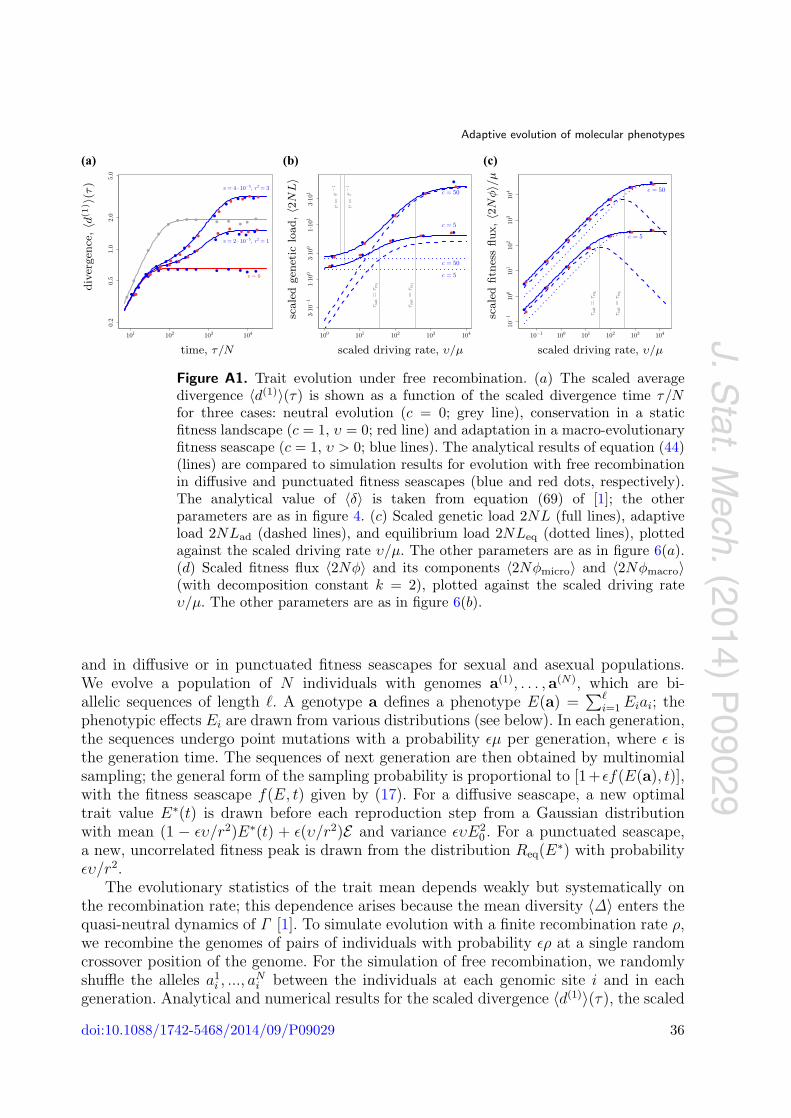
J. Stat. M

ech. (2014) P09029

Adaptive evolution of molecular phenotypes

(a) (b) (c)

Figure A1. Trait evolution under free recombination. (a) The scaled averagedivergence 〈d(1)〉(τ) is shown as a function of the scaled divergence time τ/Nfor three cases: neutral evolution (c = 0; grey line), conservation in a staticfitness landscape (c = 1, υ = 0; red line) and adaptation in a macro-evolutionaryfitness seascape (c = 1, υ > 0; blue lines). The analytical results of equation (44)(lines) are compared to simulation results for evolution with free recombinationin diffusive and punctuated fitness seascapes (blue and red dots, respectively).The analytical value of 〈δ〉 is taken from equation (69) of [1]; the otherparameters are as in figure 4. (c) Scaled genetic load 2NL (full lines), adaptiveload 2NLad (dashed lines), and equilibrium load 2NLeq (dotted lines), plottedagainst the scaled driving rate υ/μ. The other parameters are as in figure 6(a).(d) Scaled fitness flux 〈2Nφ〉 and its components 〈2Nφmicro〉 and 〈2Nφmacro〉(with decomposition constant k = 2), plotted against the scaled driving rateυ/μ. The other parameters are as in figure 6(b).

and in diffusive or in punctuated fitness seascapes for sexual and asexual populations.We evolve a population of N individuals with genomes a(1), . . . , a(N), which are bi-allelic sequences of length �. A genotype a defines a phenotype E(a) =

∑�i=1 Eiai; the

phenotypic effects Ei are drawn from various distributions (see below). In each generation,the sequences undergo point mutations with a probability εμ per generation, where ε isthe generation time. The sequences of next generation are then obtained by multinomialsampling; the general form of the sampling probability is proportional to [1+εf(E(a), t)],with the fitness seascape f(E, t) given by (17). For a diffusive seascape, a new optimaltrait value E∗(t) is drawn before each reproduction step from a Gaussian distributionwith mean (1 − ευ/r2)E∗(t) + ε(υ/r2)E and variance ευE2

0 . For a punctuated seascape,a new, uncorrelated fitness peak is drawn from the distribution Req(E∗) with probabilityευ/r2.

The evolutionary statistics of the trait mean depends weakly but systematically onthe recombination rate; this dependence arises because the mean diversity 〈Δ〉 enters thequasi-neutral dynamics of Γ [1]. To simulate evolution with a finite recombination rate ρ,we recombine the genomes of pairs of individuals with probability ερ at a single randomcrossover position of the genome. For the simulation of free recombination, we randomlyshuffle the alleles a1

i , ..., aNi between the individuals at each genomic site i and in each

generation. Analytical and numerical results for the scaled divergence 〈d(1)〉(τ), the scaled

doi:10.1088/1742-5468/2014/09/P09029 36

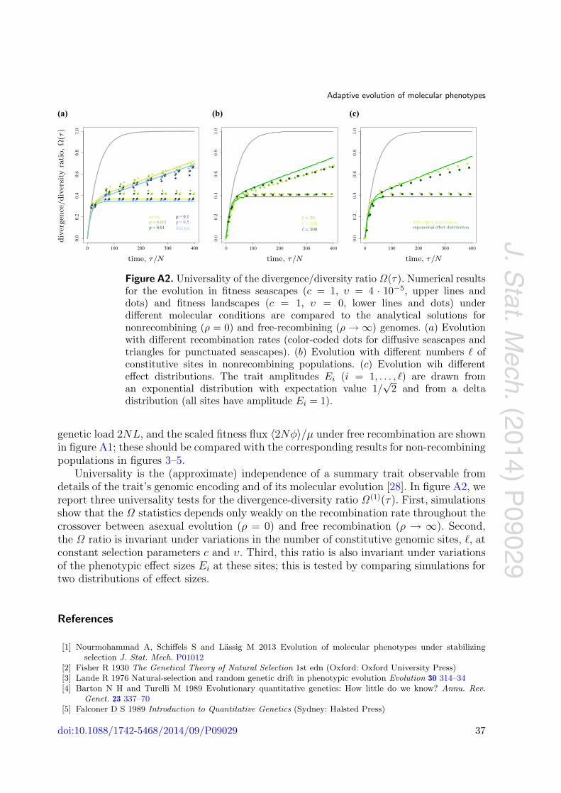
J. Stat. M

ech. (2014) P09029

Adaptive evolution of molecular phenotypes

(a) (b) (c)

Figure A2. Universality of the divergence/diversity ratio Ω(τ). Numerical resultsfor the evolution in fitness seascapes (c = 1, υ = 4 · 10−5, upper lines anddots) and fitness landscapes (c = 1, υ = 0, lower lines and dots) underdifferent molecular conditions are compared to the analytical solutions fornonrecombining (ρ = 0) and free-recombining (ρ → ∞) genomes. (a) Evolutionwith different recombination rates (color-coded dots for diffusive seascapes andtriangles for punctuated seascapes). (b) Evolution with different numbers � ofconstitutive sites in nonrecombining populations. (c) Evolution wih differenteffect distributions. The trait amplitudes Ei (i = 1, . . . , �) are drawn froman exponential distribution with expectation value 1/

√2 and from a delta

distribution (all sites have amplitude Ei = 1).

genetic load 2NL, and the scaled fitness flux 〈2Nφ〉/μ under free recombination are shownin figure A1; these should be compared with the corresponding results for non-recombiningpopulations in figures 3–5.

Universality is the (approximate) independence of a summary trait observable fromdetails of the trait’s genomic encoding and of its molecular evolution [28]. In figure A2, wereport three universality tests for the divergence-diversity ratio Ω (1)(τ). First, simulationsshow that the Ω statistics depends only weakly on the recombination rate throughout thecrossover between asexual evolution (ρ = 0) and free recombination (ρ → ∞). Second,the Ω ratio is invariant under variations in the number of constitutive genomic sites, �, atconstant selection parameters c and υ. Third, this ratio is also invariant under variationsof the phenotypic effect sizes Ei at these sites; this is tested by comparing simulations fortwo distributions of effect sizes.

References

[1] Nourmohammad A, Schiffels S and Lassig M 2013 Evolution of molecular phenotypes under stabilizingselection J. Stat. Mech. P01012

[2] Fisher R 1930 The Genetical Theory of Natural Selection 1st edn (Oxford: Oxford University Press)[3] Lande R 1976 Natural-selection and random genetic drift in phenotypic evolution Evolution 30 314–34[4] Barton N H and Turelli M 1989 Evolutionary quantitative genetics: How little do we know? Annu. Rev.

Genet. 23 337–70[5] Falconer D S 1989 Introduction to Quantitative Genetics (Sydney: Halsted Press)

doi:10.1088/1742-5468/2014/09/P09029 37

J. Stat. M

ech. (2014) P09029

Adaptive evolution of molecular phenotypes

[6] Lynch M and Walsh B 1998 Genetics and Analysis of Quantitative Traits (Sunderland: Sinauer)[7] Rice S 1990 A geometric model for the evolution of development J. Theor. Biol. 143 319–42[8] Hartl D L and Taubes C H 1996 Compensatory nearly neutral mutations: selection without adaptation

J. Theor. Biol. 182 303–9[9] Blumer M G 1972 The genetic variability of polygenic characters under optimizing selection, mutation and

drift Genet. Res. 19 17–25[10] Barton N H 1986 The maintenance of polygenic variation through a balance between mutation and stabilizing

selection Genet. Res. 47 209–16[11] Wright S 1935 The analysis of variance and the correlations between relatives with respect to deviations from

an optimum J. Genet. 30 243–56[12] Mustonen V and Lassig M 2009 From fitness landscapes to seascapes: non-equilibrium dynamics of selection

and adaptation Trends Genet. 25 111–9[13] Kopp M and Hermisson J 2009 The genetic basis of phenotypic adaptation ii: the distribution of adaptive

substitutions in the moving optimum model Genetics 183 1453–76[14] de Vladar H P and Barton N H 2011 The statistical mechanics of a polygenic character under stabilizing

selection, mutation and drift J. R. Soc. Interface 8 720–39[15] Mustonen V and Lassig M 2008 Molecular evolution under fitness fluctuations Phys. Rev. Lett. 100 108101[16] Hansen T F 1997 Stabilizing selection and the comparative analysis of adaptation Evolution 51 1341–51[17] Butler M A and King A A 2004 Phylogenetic comparative analysis: a modeling approach for adaptive

evolution Am. Nat. 164 683–95[18] Bedford T and Hartl D L 2009 Optimization of gene expression by natural selection Proc. Natl Acad. Sci.

USA 106 1133–8[19] Beaulieu J M, Jhwueng D C, Boettiger C and O’Meara B C 2012 Modeling stabilizing selection: expanding

the Ornstein–Uhlenbeck model of adaptive evolution Evolution 66 2369–83[20] Mustonen V and Lassig M 2010 Fitness flux and ubiquity of adaptive evolution Proc. Natl Acad. Sci.

107 4248–53[21] Zhao Y, Stormo G D 2011 Quantitative analysis demonstrates most transcription factors require only simple

models of specificity Nature Biotech. 29 480–3[22] Kimura M 1964 Diffusion models in population genetics J. Appl. Probab. 1 177–232[23] Ewens W J 2004 Mathematical Population Genetics (New York: Springer)[24] Berg J, Willmann S and Lassig M 2004 Adaptive evolution of transcription factor binding sites BMC Evol.

Biol. 4 42[25] Lassig M 2007 From biophysics to evolutionary genetics: statistical aspects of gene regulation BMC

Bioinformatics 8 S7[26] Neher R A and Shraiman B I 2009 Competition between recombination and epistasis can cause a transition

from allele to genotype selection Proc. Natl Acad. Sci. 106 6866–71[27] Neher R A, Vucelja M, Mezard M and Shraiman B I 2013 Emergence of clones in sexual populations J. Stat.

Mech. P01008[28] Nourmohammad A, Held T and Lassig M 2013 Universality and predictability in molecular quantitative

genetics Curr. Opin. Genet. Dev. 23 684–93[29] Mustonen V and Lassig M 2005 Evolutionary population genetics of promoters: predicting binding sites and

functional phylogenies Proc. Natl Acad. Sci. 102 15936–41[30] Barton N H and Coe J B 2009 On the application of statistical physics to evolutionary biology J. Theor.

Biol. 259 317–24[31] Barton N H and de Vladar H P 2009 Statistical mechanics and the evolution of polygenic quantitative traits

Genetics 181 997–1011[32] Neher R A and Shraiman B I 2011 Statistical genetics and evolution of quantitative traits Rev. Mod. Phys.

83 1283–300[33] Poelwijk F J, Heyning P D, de Vos M G J, Kiviet D J and Tans S J 2011 Optimality and evolution of

transcriptionally regulated gene expression BMC Syst. Biol. 5 128[34] Gerland U and Hwa T 2002 On the selection and evolution of regulatory DNA motifs J. Mol. Evol. 55 386–400[35] Mustonen V, Kinney J, Callan C G J and Lassig M 2008 Energy-dependent fitness: a quantitative model for

the evolution of yeast transcription factor binding sites Proc. Natl Acad. Sci. 105 12376–81[36] Wylie C S and Shakhnovich E I 2011 A biophysical protein folding model accounts for most mutational

fitness effects in viruses Proc. Natl Acad. Sci. 108 9916–21[37] Hermsen R, Deris J B and Hwa T 2012 On the rapidity of antibiotic resistance evolution facilitated by

a concentration gradient Proc. Natl Acad. Sci. 109 10775–80[38] Lassig M 2000 Dynamical anomalies and intermittency in Burgers turbulence Phys. Rev. Lett. 84 2618–21

doi:10.1088/1742-5468/2014/09/P09029 38

J. Stat. M

ech. (2014) P09029

Adaptive evolution of molecular phenotypes

[39] Lynch M and Force A 2000 The probability of duplicate gene preservation by subfunctionalization Genetics154 459–73 (PMC 1460895)

[40] Rivoire O and Leibler S 2014 A model for the generation and transmission of variations in evolution Proc.Natl Acad. Sci. 111 E1940–9

[41] Mohle M 2001 Forward and backward diffusion approximations for haploid exchangeable population modelsStoch. Proc. Appl. 95 133–49

[42] Nourmohammad A et al in preparation[43] Chakraborty R and Nei M 1982 Genetic differentiation of quantitative characters between populations or

species: I. Mutation and random genetic drift Genet. Res. Camb. 39 303–14[44] Lynch M and Hill W G 1986 Phenotypic evolution by neutral mutation Evolution 40 915–35[45] Lynch M and Walsh B 1998 Genetics and Analysis of Quantitative Traits (Sunderland: Sinauer) chapter 12[46] Crow J F 1958 Some possibilities for measuring selection intensities in man Human Biol. 30 1–13[47] Crow J F and Kimura M 1965 Evolution in sexual and asexual populations Am. Naturalist 99 439–50[48] Haldane J B S 1957 The cost of natural selection J. Genet. 55 511–24[49] Muller H J 1950 Our load of mutations Am. J. Human Genet. 2 111–76[50] Hartl D L and Taubes C H 1998 Towards a theory of evolutionary adaptation Genetica 102–103 525–33[51] Poon A and Otto S P 2000 Compensating for our load of mutations: freezing the meltdown of small

populations Evolution 54 1467–79[52] Tenaillon O, Silander O K, Uzan J-P and Chao L 2007 Quantifying organismal complexity using a population

genetic approach PloS One 2 e217[53] Mustonen V and Lassig M 2007 Adaptations to fluctuating selection in Drosophila Proc. Natl Acad. Sci.

104 2277–82[54] Chernyak V Y, Chertkov M and Jarzynski C 2006 Path-integral analysis of fluctuation theorems for general

Langevin processes J. Stat. Mech. 8 080001[55] Strelkowa N and Lassig M 2012 Clonal interference in the evolution of influenza Genetics 192 671–82[56] Schiffels S, Szollosi G J, Mustonen V and Lassig M 2011 Emergent neutrality in adaptive asexual evolution

Genetics 189 1361–75[57] �Luksza M and Lassig M 2014 A predictive fitness model for influenza Nature 507 57–61[58] Tenaillon O, Rodrıguez-Verdugo A, Gaut R L, McDonald P, Bennett A F, Long A D and Gaut B S 2012

The molecular diversity of adaptive convergence Science 335 457–61[59] Toprak E, Veres A, Michel J B, Chait R, Hartl D L and Kishony R 2012 Evolutionary paths to antibiotic

resistance under dynamically sustained drug selection Nature Genet. 44 101–5[60] Barroso-Batista J, Sousa A, Lourenco M, Bergman M L, Sobral D, Demengeot J, Xavier K B and Gordo I

2014 The first steps of adaptation of escherichia coli to the gut are dominated by soft sweeps PLoS Genet.10 e1004182

[61] Khaitovich P, Hellmann I, Enard W, Nowick K, Leinweber M, Franz H, Weiss G, Lachmann M and Paabo S2005 Parallel patterns of evolution in the genomes and transcriptomes of humans and chimpanzees Science309 1850–4

[62] Gilad Y, Oshlack A, Smyth G K, Speed T P and White K P 2006 Expression profiling in primates reveals arapid evolution of human transcription factors Nature 440 242–5

[63] Fraser H B 2011 Genome-wide approaches to the study of adaptive gene expression evolution BioEssays33 469–77

[64] McDonald J H and Kreitman M 1991 Adaptive protein evolution at the Adh locus in Drosophila Nature351 652–4

[65] Smith N G C and Eyre-Walker A 2002 Adaptive protein evolution in Drosophila Nature 415 1022–4[66] Szendro I G, Franke J, de Visser J A G M and Krug J 2013 Predictability of evolution depends

nonmonotonically on population size Proc. Natl Acad. Sci. 110 571–6[67] Gardiner C 2004 Handbook of Stochastic methods: for Physics, Chemistry and the Natural Sciences 3rd edn

(Berlin: Springer)

doi:10.1088/1742-5468/2014/09/P09029 39