ADAPTIVE HYBRIDIZED INTERIOR PENALTY DISCONTINUOUSGALERKIN METHODS FOR H(CURL)-ELLIPTIC PROBLEMS

C. CARSTENSEN∗† , R. H. W. HOPPE‡§ , N. SHARMA‡ , AND T. WARBURTON¶‖

Abstract. We develop and analyze an adaptive hybridized Interior Penalty DiscontinuousGalerkin (IPDG-H) method for H(curl)- elliptic boundary value problems in 2D or 3D arising from asemi-discretization of the eddy currents equations. The method can be derived from a mixed formula-tion of the given boundary value problem and involves a Lagrange multiplier that is an approximationof the tangential traces of the primal variable on the interfaces of the underlying triangulation ofthe computational domain. It is shown that the IPDG-H technique can be equivalently formulatedand thus implemented as a mortar method. The mesh adaptation is based on a residual-type aposteriori error estimator consisting of element and face residuals. Within a unified framework foradaptive finite element methods, we prove the reliability of the estimator up to a consistency error.The performance of the adaptive symmetric IPDG-H method is documented by numerical results forrepresentative test examples in 2D.

Key words. adaptive hybridized Interior Penalty Discontinuous Galerkin method, a posteriorierror analysis, H(curl)-elliptic boundary value problems, semi-discrete eddy currents equations

AMS subject classifications. 65F10, 65N30

1. Introduction. Discontinuous Galerkin (DG) methods are widely used algo-rithmic schemes for the numerical solution of partial differential equations (PDE).For a comprehensive description, we refer to the survey article [24] and the refer-ences therein. As far as elliptic boundary value problems are concerned, DG methodscan be derived from a primal-dual mixed formulation using local approximations ofthe primal and dual variables by polynomial scalar and vector-valued functions andappropriately designed numerical fluxes. Among the most popular schemes are Inte-rior Penalty DG (IPDG) and Local DG (LDG) methods which have been analyzedby means of a priori estimates of the global discretization, e.g., in [3, 5, 23, 39].For H(curl)-elliptic boundary value problems arising from a semi-discretization of theeddy currents equations, symmetric IPDG methods have been studied in [36]. Thetime-harmonic Maxwell equations have been addressed in [46].On the other hand, the a posteriori error analysis and application of adaptive finiteelement methods (FEM) for the efficient numerical solution of boundary and initial-boundary value problems for PDE has reached some state of maturity as documentedby a series of monographs. There exist several concepts including residual and hi-erarchical type estimators, error estimators that are based on local averaging, theso-called goal oriented dual weighted approach, and functional type error majorants(cf. [2, 6, 7, 30, 44, 49] and the references therein). A posteriori error estimators forDG methods applied to second order elliptic boundary value problems have been de-veloped and analyzed in [1, 11, 18, 38, 40, 47]. In particular, a convergence analysis ofadaptive symmetric IPDG methods has been provided in [12, 34] and [41]. Residual-and hierarchical-type a posteriori error estimator for H(curl)-elliptic problems have

∗Dep. of Math., Humboldt Universitat zu Berlin, D-10099 Berlin, Germany†Dep. of Comput. Sci. Eng., Yonsei University, Seoul 120-749, Korea‡Dep. of Math., Univ. of Houston, Houston, TX 77204-3008, U.S.A.§Inst. of Math., Univ. of Augsburg, D-86159 Augsburg, Germany¶CAAM, Rice Univ., Houston, TX 77005-1892, U.S.A.‖The first author has been supported by the German National Science Foundation DFG within

the Research Center MATHEON and by the WCU program through KOSEF (R31-2008-000-10049-0). The other authors acknowledge support by the NSF grant DMS-0810176

1

been studied in [8, 9, 10, 20, 37]. A convergence analysis for residual estimators hasbeen developed in [19] for 2D and in [35] for 3D problems.From a computational point of view, DG methods suffer from a relatively hugeamount of globally coupled degrees of freedom (DOF) compared to standard FEM.Hybridization is a technique that gives rise to a significant reduction of the globallycoupled DOF. It has been introduced for mixed FEM in [31] and further studied in[4, 13, 15, 25, 26]. Adaptive mixed hybrid methods on the basis of reliable a posteriorierror estimators have been considered in [14, 45] and [50]. For DG methods, a surveyof hybridized DG (DG-H) methods has been provided in [26], whereas a unified anal-ysis has been developed in [28]. However, adaptive DG-H methods have not yet beeninvestigated.

In this paper, we will derive and analyze a residual-type a posteriori error esti-mator for hybridized symmetric IPDG (IPDG-H) methods applied to H(curl)-ellipticboundary value problems in 3D. The analysis will be carried out within a unifiedframework provided for adaptive finite element approximations in [17, 18, 20, 21, 22].The paper is organized as follows: In Section 2, we introduce some basic notationand present the class of H(curl)-elliptic boundary value problems to be approximatedby symmetric IPDG-H methods. Section 3 deals with the development of symmetricIPDG-H methods based on a mixed formulation of the elliptic boundary value prob-lems. We establish its relationship with mortar techniques which allows the imple-mentation as a mortar method. In section 4, we present the residual-type a posteriorierror estimator and prove its reliability. Finally, in section 5, we provide a detaileddocumentation of numerical results to illustrate the performance of the symmetricIPDG-H methods.

2. Basic Notations. Let Ω ⊂ R3 be a simply connected polyhedral domainwith boundary Γ = ∂Ω such that Γ = ΓD ∪ ΓN ,ΓD ∩ ΓN = ∅. We denote byD(Ω) the space of all infinitely often differentiable functions with compact supportin Ω and by D′(Ω) its dual space referring to < ·, · > as the dual pairing betweenD′(Ω) and D(Ω). We further adopt standard notation from Lebesgue and Sobolevspace theory. In particular, for a subset D ⊂ Ω, we refer to L2(D) and L2(D) asthe Hilbert spaces of scalar and vector-valued square integrable functions with innerproducts (·, ·)0,D and associated norms ‖ · ‖0,D, respectively. Further, we denote byH1(D) the Sobolev space of square integrable functions with square integrable weakderivatives equipped with the inner product (·, ·)1,D and norm ‖ · ‖1,D. For Σ ⊆ ∂D,we refer to H1/2(Σ) as the space of traces v|Σ of functions v ∈ H1(D) on Σ. We setH1

0,Σ(D) := v ∈ H1(Ω)|v|Σ = 0 and refer to H−1Σ (D) as the associated dual space.

For a simply connected polyhedral domain Ω with boundary Γ = ∂Ω which can besplit into J relatively open faces Γ1, . . . , ΓJ with Γ = ∪J

j=1Γj , we refer to H(curl; Ω)as the Hilbert space H(curl; Ω) := u ∈ L2(Ω) | curl u ∈ L2(Ω), equipped withthe inner product (u,v)curl,Ω := (u,v)0,Ω + (curl u, curl v)0,Ω and the associatednorm ‖ · ‖curl,Ω. We further refer to H(curl0; Ω) as the subspace of irrotationalvector fields. The space H(div; Ω) is defined by H(div; Ω) := q ∈ L2(Ω) | div q ∈L2(Ω) which is a Hilbert space with respect to the inner product (u,v)div,Ω :=(u,v)0,Ω + (div u, div v)0,Ω and the associated norm ‖ · ‖div,Ω. For vector fieldsu ∈ C∞(Ω)3 := u|Ω | u ∈ C∞(R3), the normal component trace reads ηn(u)|Γj :=nΓj · u|Γj , j = 1, . . . , J with the exterior unit normal vector nΓj on Γj . The normalcomponent trace mapping can be extended by continuity to a surjective, continuouslinear mapping ηn : H(div; Ω) → H−1/2(Γ) (cf. [32]; Thm. 2.2). We defineH0(div; Ω) as the subspace of vector fields with vanishing normal components on

2

Γ. In order to study the traces of vector fields q ∈ H(curl; Ω), following [16], weintroduce the spaces

L2t(Γ) := u ∈ L2(Ω) | ηn(u) = 0,

H1/2− (Γ) := u ∈ L2

t(Γ) | u|Γj ∈ H1/2(Γj) for all j = 1, . . . , J.

¡¡

¡¡

¡¡

¡¡¡

@@

@@

@@

@@@Γj Γk?

©©©*HHHYtj tk

tjk

ZZ

Z½

½½>

nj nk

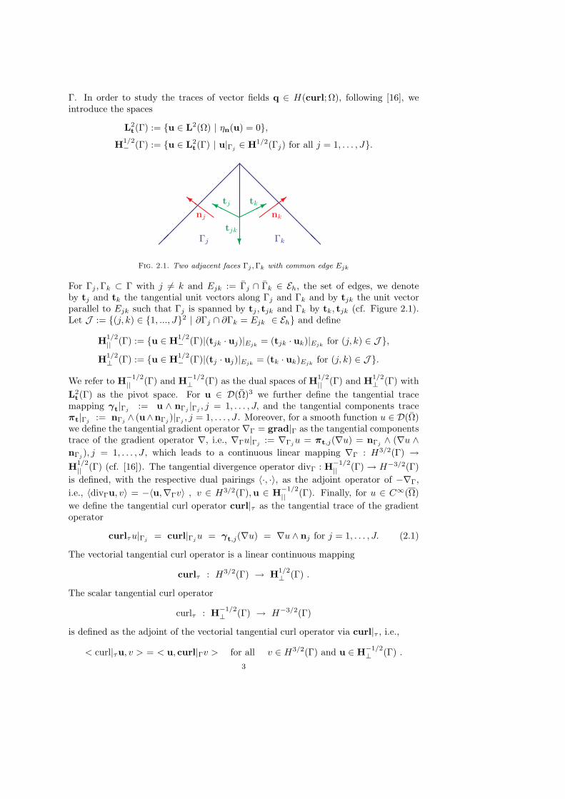
Fig. 2.1. Two adjacent faces Γj , Γk with common edge Ejk

For Γj , Γk ⊂ Γ with j 6= k and Ejk := Γj ∩ Γk ∈ Eh, the set of edges, we denoteby tj and tk the tangential unit vectors along Γj and Γk and by tjk the unit vectorparallel to Ejk such that Γj is spanned by tj , tjk and Γk by tk, tjk (cf. Figure 2.1).Let J := (j, k) ∈ 1, ..., J2 | ∂Γj ∩ ∂Γk = Ejk ∈ Eh and define

H1/2|| (Γ) := u ∈ H1/2

− (Γ)|(tjk · uj)|Ejk= (tjk · uk)|Ejk

for (j, k) ∈ J ,H1/2⊥ (Γ) := u ∈ H1/2

− (Γ)|(tj · uj)|Ejk= (tk · uk)Ejk

for (j, k) ∈ J .

We refer to H−1/2|| (Γ) and H−1/2

⊥ (Γ) as the dual spaces of H1/2|| (Γ) and H1/2

⊥ (Γ) withL2

t(Γ) as the pivot space. For u ∈ D(Ω)3 we further define the tangential tracemapping γt|Γj := u ∧ nΓj |Γj , j = 1, . . . , J, and the tangential components traceπt|Γj := nΓj ∧ (u∧nΓj )|Γj , j = 1, . . . , J . Moreover, for a smooth function u ∈ D(Ω)we define the tangential gradient operator ∇Γ = grad|Γ as the tangential componentstrace of the gradient operator ∇, i.e., ∇Γu|Γj := ∇Γj u = πt,j(∇u) = nΓj ∧ (∇u ∧nΓj ), j = 1, . . . , J , which leads to a continuous linear mapping ∇Γ : H3/2(Γ) →H1/2|| (Γ) (cf. [16]). The tangential divergence operator divΓ : H−1/2

|| (Γ) → H−3/2(Γ)is defined, with the respective dual pairings 〈·, ·〉, as the adjoint operator of −∇Γ,i.e., 〈divΓu, v〉 = −〈u,∇Γv〉 , v ∈ H3/2(Γ),u ∈ H−1/2

|| (Γ). Finally, for u ∈ C∞(Ω)we define the tangential curl operator curl|τ as the tangential trace of the gradientoperator

curlτu|Γj = curl|Γj u = γt,j(∇u) = ∇u ∧ nj for j = 1, . . . , J. (2.1)

The vectorial tangential curl operator is a linear continuous mapping

curlτ : H3/2(Γ) → H1/2⊥ (Γ) .

The scalar tangential curl operator

curlτ : H−1/2⊥ (Γ) → H−3/2(Γ)

is defined as the adjoint of the vectorial tangential curl operator via curl|τ , i.e.,

< curl|τu, v > = < u, curl|Γv > for all v ∈ H3/2(Γ) and u ∈ H−1/2⊥ (Γ) .

3

The range spaces of the tangential trace mapping γt and the tangential componentstrace mapping πt on H(curl; Ω) can be characterized by means of the spaces

H−1/2(div|Γ, Γ) := λ ∈ H−1/2|| (Γ) | div|Γλ ∈ H−1/2(Γ) ,

H−1/2(curl|Γ, Γ) := λ ∈ H−1/2⊥ (Γ) | curl|Γλ ∈ H−1/2(Γ) ,

which are dual to each other with respect to the pivot space L2t(Γ). We refer to

‖ · ‖−1/2,divΓ,Γ and ‖ · ‖−1/2,curlΓ,Γ as the respective norms and denote by 〈·, ·〉−1/2,Γ

the dual pairing (see, e.g., [16] for details).It can be shown that the tangential trace mapping is a continuous linear mapping

γt : H(curl; Ω) → H−1/2(div|Γ, Γ) ,

whereas the tangential components trace mapping is a continuous linear mapping

πt : H(curl; Ω) → H−1/2(curl|Γ, Γ) .

The previous results imply that the tangential divergence of the tangential traceand the scalar tangential curl of the tangential components trace coincide: For u ∈H(curl; Ω) it holds divΓ (u ∧ n) = curl|Γ (n ∧ (u ∧ n)) = n · curl u. We defineH0(curl; Ω) as the subspace of H(curl; Ω) with vanishing tangential traces on Γ.

Given a polyhedral domain Ω ⊂ R3 with boundary Γ = ∂Ω such that Γ =ΓD ∪ ΓN , ΓD ∩ ΓN = ∅, we denote by TH(Ω) a shape-regular simplicial triangulationof Ω that aligns with ΓD and ΓN . We refer to FH(Ω) as the set of interior facesF = T+ ∩ T−, T± ∈ TH(Ω), and to FH(Σ) as the set of faces located on the boundaryΣ ⊆ Γ, while FH(Ω) := FH(Ω)∪FH(Γ) is the set of all faces. Further, EH(Σ) standsfor the set of edges on Σ. We denote by hT and hF the diameter of an elementT ∈ TH(Ω) and a face F ∈ FH(Ω), respectively. For two quantities A,B ∈ R+, weuse the notation A . B, if there exists a constant C ∈ R+, independent of the meshsize of the triangulation TH(Ω), such that A ≤ CB.We refer to

Nd1(Ω; TH(Ω)) := vH ∈ H(curl; Ω) | vH |T ∈ ND1(T ) , T ∈ TH(Ω)as the curl-conforming edge element space, where ND1(T ) stands for the lowest orderedge element of Nedelec’s first family [43], and to

Nd10,ΓD

(Ω; TH(Ω)) := vH ∈ Nd1(Ω; TH(Ω)) | γt(vH) = 0 on ΓDas its subspace of vanishing tangential trace components on ΓD.For vector fields vH ∈ ∏

T∈TH(Ω) H(curl; T ), we denote by ‖ · ‖curl,H,Ω the mesh-dependent norm

‖vH‖curl,H,Ω :=( ∑

T∈TH(Ω)

(‖vH‖20,T + ‖curl vH‖20,T

))1/2

.

Moreover, for such vector fields we set v±H |F := (vH |T±)|F along F = T+∩T− ∈ FH(Ω)and define

vH :=

(v+H + v−H)/2 , F ∈ FH(Ω)

vH , F ∈ FH(Γ) ,

[vH ] :=

v+H − v−H , F ∈ FH(Ω)

0 , F ∈ FH(Γ)

4

as the averages and jumps of vH across the interior faces F of the triangulation.For scalar functions vH ∈ L2(Ω), the averages vH and jumps [vH ] are definedanalogously.

The class of H(curl)-elliptic boundary value problems to be approximated byIPDG-H methods is of the form

curl µ−1 curl u + σ u = f in Ω, (2.2a)γt(u) = g1 on ΓD, (2.2b)

πt(µ−1curl u) = g2 on ΓN . (2.2c)

We assume that f ∈ L2(Ω),g1 ∈ L2(ΓD), and g2 ∈ H(curl0ΓN; ΓN ). We further

suppose that µ is a symmetric, uniformly positive definite matrix-valued functionµ = µ(x), x ∈ Ω, and that σ is a scalar nonnegative function σ = σ(x), x ∈ Ω, thatare elementwise constant with respect to a given coarse simplicial triangulation TH(Ω)of the computational domain.We note that the subsequent analysis also applies to H(curl)-elliptic problems in 2Das given by

curl µ−1 curl u + σ u = f in Ω , (2.3a)tΓD

· u = g1 on ΓD, (2.3b)

µ−1 curl u = g2 on ΓN , (2.3c)

where curl u = ∂u2/∂x1 − ∂u1/∂x2 for u = (u1, u2)T , whereas curl u = (∂u/∂x2,−∂u/∂x1)T for a scalar function u. Moreover, tΓD

stands for the tangential unitvector on the Dirichlet part ΓD of the boundary. The data f , g1 and g2 have to bechosen accordingly.We will develop the IPDG-H method and perform the a posteriori error analysis onlyin the 3D case. The necessary modifications for 2D problems are straightforward.

3. Hybridized IPDG Methods. A mixed formulation of (2.2a)-(2.2c) can bederived by introducing p := µ−1curl u as an additional variable. Setting

V := v ∈ H(curl; Ω) | γt(u) = g1 on ΓD , Q := L2(Ω), (3.1)V0 := v ∈ H(curl; Ω) | γt(u) = 0 on ΓD,

it amounts to the computation of (u,p) ∈ V ×Q with

a(p,q) − b(u,q) = `(1)(q) for all q ∈ Q, (3.2a)

b(v,p) + c(u,v) = `(2)(v) for all v ∈ V0. (3.2b)

5

The bilinear forms a, b and c and the functionals `(1) ∈ Q∗, `(2) ∈ V∗0 are given by

a(p,q) :=∫

Ω

µ p · q dx , (3.3a)

b(u,q) :=∫

Ω

curl u · q dx , (3.3b)

c(u,v) :=∫

Ω

σ u · v dx , (3.3c)

`(1)(q) := 0 , (3.3d)

`(2)(v) :=∫

Ω

f · v dx +∫

ΓN

g2 · γt(v) dτ. (3.3e)

The operator-theoretic framework involves the operator A : (V ×Q) → (V0 ×Q)∗

defined, for all (u,p) ∈ V ×Q and all (v,q) ∈ V0 ×Q by

(A(u,p))(v,q) := a(p,q)− b(u,q) + b(v,p) + c(u,v). (3.4)

Then, the system (3.2a)-(3.2b) can be written in compact form as

A(u,p) = `, (3.5)

where `(v,q) := `(1)(q) + `(2)(v) for all (v,q) ∈ V0 ×Q.

Theorem 3.1. Under the assumptions on the data of (2.2a)-(2.2c), A is acontinuous, bijective linear operator. Hence, for any (`(1), `(2)) ∈ Q∗×V∗

0, the system(3.2a)-(3.2b) admits a unique solution (u,p) ∈ V×Q which continuously depends onthe data, namely

‖(u,p)‖V×Q . ‖`(1)‖Q∗ + ‖`(2)‖V ∗0 . (3.6)

Proof. The mapping properties are straightforward. If g1 6= 0, there exists aunique ug1 ∈ V such that for all v ∈ V0 (cf., e.g., [42])

(A(ug1 ,0))(v,−µ−1curl v) =∫

Ω

(µ−1curl ug1 · curl v + σug1 · v

)dx = 0,

and hence, we may restrict ourselves to the case of A : V0 ×Q → (V0 ×Q)∗. Now,for any (u,p) ∈ V0 ×Q we have

(A(u,p))(3u, 2p− µ−1curl u) = (A(3u, 2p + µ−1curl u))(u,p)

= 2µ‖p‖2L2(Ω) + 3σ‖u‖2L2(Ω) + µ−1‖curl u‖2L2(Ω).

This implies the inf-sup condition and the remaining degeneracy condition whichimplies bijectivity.

Given a simplicial triangulation TH(Ω), DG methods are based on the approxi-mation of the vector field u and p by elementwise polynomials, thus giving rise to the

6

finite dimensional function spaces

VH := vH ∈ L2(Ω) | vH |T ∈ (Πk(T )) , T ∈ TH(Ω), (3.7a)γt(vH) = gH,1 on F ∈ FH(ΓD),

QH := qH ∈ L2(Ω) | qH |T ∈ Πk(T ) , T ∈ TH(Ω). (3.7b)

Here and in the sequel, gH,1 ∈ Πk(F ), F ∈ FH(ΓD) is some approximation of g1 andΠk(T ), T ∈ TH(Ω), as well as Πk(F ), F ∈ FH(Ω), stand for the sets of vector-valuedfunctions whose components are polynomials of degree at most k ∈ N.DG methods amount to the computation of (pH ,uH) ∈ QH ×VH with

aH(pH ,qH) − bH(uH ,qH) + dH(uH ,qH) = `(1)H (qH) for all qH ∈ QH , (3.8a)

bH(vH ,pH) − dH(vH , pH) + cH(uH ,vH) = `(2)H (vH) for all vH ∈ VH . (3.8b)

Here and throughout, uH , pH are appropriate numerical flux functions and the mesh-dependent bilinear forms aH , bH , cH , and dH are defined by means of

aH(pH ,qH) :=∑

T∈TH(Ω)

∫

T

µpH · qH dx, (3.9a)

bH(uH ,qH) :=∑

T∈TH(Ω)

∫

T

curl uH · qH dx, (3.9b)

cH(uH ,vH) :=∑

T∈TH(Ω)

∫

T

σuH · vH dx, (3.9c)

dH(uH ,qH) :=∑

F∈FH(Ω)

〈γt(uH), πt(qH)〉. (3.9d)

The functionals `(1)H and `

(2)H are given by

`(1)H (qH) := 0, (3.10a)

`(2)H (vH) :=

∑

T∈TH(Ω)

∫

T

f · vH dx +∑

F∈FH(ΓN )

∫

F

g2 · γt(vH) dτ. (3.10b)

In case of symmetric Interior Penalty Discontinuous Galerkin (IPDG) methods, thenumerical fluxes read

γt(uH) := γt(uH) , F ∈ FH(Ω)

0 , F ∈ FH(Γ) (3.11a)

πt(pH) := πt(µ−1curl uH) − α h−1

F [γt(uH)] , F ∈ FH(Ω)0 , F ∈ FH(Γ) (3.11b)

with a suitable penalty parameter α > 0. The choice qH := µ−1curl vH in (3.8a)and (3.11a),(3.11b) allow the elimination of pH from (3.8a),(3.8b). This results in thefollowing standard form of the symmetric IPDG method: Find uH ∈ VH such that

aIP (uH ,vH) = `IP (vH) for all vH ∈ VH . (3.12)7

Here and in the sequel, the bilinear form aIP and the functional `IP read

aIP (uH ,vH) :=∑

T∈TH(Ω)

∫

T

(µ−1curl uH · curl vH + σuH · vH

)dx (3.13a)

−∑

F∈FH(Ω)

∫

F

(πt(µ−1curl uH) · [γt(vH)] + γt(uH) · [πt(µ−1curl vH)]

)dτ

+ α∑

F∈FH(Ω)

h−1F

∫

F

[γt(uH)] · [γt(vH)]dτ,

`IP (vH) :=∑

T∈TH(Ω)

∫

T

f · vH dx +∑

F∈FH(ΓN )

∫

F

g2 · γt(vH) dτ. (3.13b)

The idea of hybridization is to enforce the continuity of the tangential componenttraces of pH across the interior edges of the triangulation by a piecewise polynomialLagrange multiplier which is an approximation of the tangential traces of u. For thispurpose, we introduce the multiplier space

MH := µH ∈ L2(FH(Ω)) | µH |F ∈ Πk(F ) , F ∈ FH(Ω). (3.14)

Choosing a numerical flux function pH , not necessarily the same as in (3.11b), theIPDG-H method is to find (pH ,uH , λH) ∈ QH ×VH ×MH with

aH(pH ,qh) − bH(uH ,qH) + dH(λH ,qH) = `(1)H (qH) for all qH ∈ QH , (3.15a)

bH(vH ,pH) − dH(vH , pH) + cH(uH ,vH) = `(2)H (vH) for all vH ∈ VH , (3.15b)

dH(µH , pH) = 0 for all µH ∈ MH . (3.15c)

In IPDG-H methods, the penalty parameter α is typically chosen elementwise, i.e.,α|T = αT , T ∈ TH(Ω), so that on F ∈ FH(Ω) with F = T+ ∩ T−, T± ∈ TH(Ω), wehave to distinguish between α+ := αT+ and α− := αT− .The advantage of hybridized methods is that the primal and dual variables uH and pH

can be eliminated from (3.15a)-(3.15c) which results in a global variational problemfor the Lagrange multiplier λH ∈ MH of the form

a(S)H (λH , µH) = `

(S)H (µH) for all µH ∈ MH . (3.16)

Once λH ∈ MH has been computed, the primal and dual variables can be computedby the solution of low-dimensional, local problems. To this end, following the unifiedframework from [28], we set

λH =

uH on ∂T \ ΓD

0 on ∂T ∩ ΓD, gH,1 =

0 on ∂T \ ΓD

gH,1 on ∂T ∩ ΓD,

gH,2 =

0 on ∂T \ ΓN

gH,2 on ∂T ∩ ΓN

with an approximation gH,2 ∈ Πk(F ), F ∈ FH(ΓN ), of g2. We define

(Spf ,Suf) ∈ Πk(T )2 , (SpλH ,SuλH) ∈ Πk(T )2,

(SpgH,1,SugH,1) ∈ Πk(T )2 , (SpgH,2,SugH,2) ∈ Πk(T )2

8

as the solutions of the local problems

µ Spf − curl Suf = 0 in T, (3.17a)curl Spf + σ Suf = f in T,

γt(Suf) = 0 on ∂T,

µ SpλH − curl SuλH = 0 in T, (3.17b)curl SpλH + σ SuλH = 0 in T,

γt(SuλH) = λH on ∂T,

µ SpgH,1 − curl SugH,1 = 0 in T, (3.17c)curl SpgH,1 + σ SugH,1 = 0 in T,

γt(SugH,1) = gH,1 on ∂T,

µ SpgH,2 − curl SugH,2 = 0 in T, (3.17d)curl SpgH,2 + σ SugH,2 = 0 in T,

πt(SugH,2) = gH,2 on ∂T.

The numerical flux πt(pH) is given by means of local numerical fluxes

πt(pH) = Spf + SpλH + SpgH,1 + SpgH,2. (3.18)

In particular, for the IPDG-H method (3.15a)-(3.15c) we choose

Spf =

πt(µ−1curl Suf)− αT h−1F γt(Suf) on F ∈ FH(Ω ∪ ΓD),

πt(µ−1curl Suf)− αT h−1F πt(µ−1curl Suf) on F ∈ FH(ΓN ),

(3.19a)

SpλH =

πt(µ−1curl SuλH)−αT h−1

F (γt(SuλH)− λH) on F ∈ FH(Ω ∪ ΓD),πt(µ−1curl SuλH)−αT h−1

F (πt(µ−1curl SuλH)− λH) on F ∈ FH(ΓN ),

(3.19b)

SpgH,i =

πt(µ−1curl SugH,i)−αT h−1

F (γt(SugH,i)− gH,i) on F ∈ FH(Ω ∪ ΓD),πt(µ−1curl SugH,i)−αT h−1

F (πt(µ−1curl SugH,i)− gH,i) on F ∈ FH(ΓN ).

(3.19c)

For sufficiently large αT , T ∈ TH(Ω), both the local problems (3.17a)-(3.17d) and theglobal variational problem (3.16) have unique solutions which can be shown alongthe same lines of proof as in [28] for standard second order elliptic boundary valueproblems. If λH ∈ MH solves (3.16), then

pH = Spf + SpλH + SpgH,1 + SpgH,2, (3.20)uH = Suf + SuλH + SugH,1 + SugH,2

defines the solution of (3.15a)-(3.15c).

Theorem 3.2. Assume that the numerical flux pH is given by (3.18) and that(pH ,uH , λH) is the solution of (3.15a)-(3.15c). Then, the numerical flux pH and the

9

multiplier λH satisfy

πt(pH) :=

α−1(α−πt(µ−1

+ curl u+H) + α+πt(µ−1

− curl u−H)

− α+α−h−1F [γt(uH)]

)on F ∈ FH(Ω),

0 on F ∈ FH(ΓD),0 on F ∈ FH(ΓN ),

(3.21a)

λH =

α−1(α+γt(u

+H) + α− γt(u

−H)

− hF [πt(µ−1curl uH)])

on F ∈ FH(Ω),

−α−1T hF πt(µ−1curl uH) on F ∈ FH(ΓD),

−α−1T hF πt(µ−1curl uH) on F ∈ FH(ΓN ),

(3.21b)

where α := α+ + α− on F = ∂T+ ∩ ∂T− for T± ∈ TH(Ω).Proof. Let F ∈ FH(Ω). If we use (3.19a)-(3.19c) and (3.20) in (3.18), we obtain

πt(pH) = πt(µ−1curl uH) − αT h−1F

(γt(uH)− γt(SuλH)

)on F.

Hence, observing (3.17b), it follows that

[πt(pH)] = [πt(µ−1 curl uH)] −(α+ h−1

F γt(u+H) (3.22)

+ α− h−1F γt(u

−H)

)+ (α+ + α−) h−1

F λH .

The specification (3.14) of the multiplier space MH and equation (3.15c) imply[πt(pH)] = 0. This results in (3.21b) due to (3.22). On the other hand,

πt(p±H) = πt(p±H) − α±h−1F

(γt(u

±H)− λH

). (3.23)

We deduce (3.21a) by inserting (3.21b) into (3.23). The proof of (3.21a),(3.21b) forF ∈ FH(ΓD) and F ∈ FH(ΓN ) follows from similar arguments.

The representation (3.21b) of the Lagrange multiplier λH shows that it provides anapproximation of the tangential trace on the interfaces F ∈ FH(Ω) which reminds ofmortar methods for H(curl)-elliptic problems (cf., e.g., [20, 51]). Indeed, the IPDG-H method (3.15a)-(3.15c) can be equivalently formulated as a mortar method. Tosee this, choose qH = µ−1curl uH in (3.15a) and the numerical flux pH in (3.15a)according to (3.21b). Then, by elimination of pH ,

λH := λH − α−1(α+γt(u+H) + α−γt(u

−H))

satisfies

aH(uH ,vH) + bH(λH ,vH) = `(2)H (vH) for all vH ∈ VH , (3.24)

bH(µH ,uH)− dH(λH , µH) = 0 for all µH ∈ MH .

10

Here and throughout the following, the bilinear forms aH , bH and dH read

aH(uH ,vH) :=∑

T∈TH(Ω)

∫

T

(µ−1curl uH · curl vH + σuH · vH

)dx

−∑

T∈TH(Ω)

∫

∂T∩Ω

α−1αT πt(µ−1curl uH) · γt(vH) dτ

+∑

T∈TH(Ω)

∫

∂T∩Ω

α−1 αT αT ′ h−1F γt(uH) · γt(vH) dτ

−∑

T∈TH(Ω)

∫

∂T∩Ω

α−1αT γt(u+H) · πt(µ−1curl vH) dτ

+∑

T∈TH(Ω)

∫

∂T∩Γ

α−1T hF πt(µ−1curl uH) · πt(µ−1curl vH) dτ,

bH(λH ,vH) := −∑

F∈FH(Ω)

∫

F

λH · [πt(µ−1curl vH)] dτ,

dH(λH ,µH) :=∑

F∈FH(Ω)

∫

F

α h−1F λH · µH dτ.

The variational system (3.24) represents a symmetric saddle point problem which canbe solved as in the standard mortar approach. Denoting by AH , BH , DH the matricesand by bH the vector associated with the bilinear forms and the right-hand side inthe first equation of (3.24), the algebraic form of the saddle point problem is

(AH BH

BTH −DH

)(uH

λH

)=

(bH

0

). (3.25)

Static condensation of uH results in the equivalent Schur complement system

(DH + BT

HA−1H BH

)λH = BT

HA−1H bH . (3.26)

4. A posteriori error analysis. The residual a posteriori error estimator forthe symmetric IPDG-H method (3.15a)-(3.15c) is given by

η :=( ∑

T∈TH(Ω)

(η2

T,1 + η2T,2 + η2

T,3

)+

∑

F∈FH(Ω)

(η2

F,1 + η2F,2

)(4.1)

+∑

F∈FH(ΓN )

(η2

F,3 + η2F,4

))1/2

.

They consist of the element residuals

ηT,1 := ‖µpH − curl uH‖0,T for all T ∈ TH(Ω), (4.2a)ηT,2 := hT ‖f − curl pH − σuH‖0,T for all T ∈ TH(Ω), (4.2b)ηT,3 := hT ‖∇ · (f − σuH)‖0,T for all T ∈ TH(Ω), (4.2c)

11

and the face residuals

ηF,1 := h1/2F ‖[πt(pH)]‖0,F for all F ∈ FH(Ω), (4.3a)

ηF,2 := h1/2F ‖nF · [f − σuH ]‖0,F for all F ∈ FH(Ω), (4.3b)

ηF,3 := h1/2F ‖g2 − πt(pH)‖0,F for all F ∈ FH(ΓN ), (4.3c)

ηF,4 := h1/2F ‖nF · (f − σuH)‖0,F for all F ∈ FH(ΓN ). (4.3d)

The nonconformity of the symmetric IPDG-H method results in some consistencyerror

ξ := minvH∈V

( ∑

T∈TH(Ω)

(‖uH − vH‖20,T + ‖curl (uH − vH)‖20,T ))1/2

(4.4)

with the unique minimizer uH ∈ V of (4.4) and ξ2 = ‖uH − uH‖20,Ω + ‖curl(uH −uH)‖20,Ω.

Theorem 4.1. Let (p,u) ∈ Q×V and (pH ,uH ,λH) ∈ QH ×VH ×MH be thesolutions of (3.5) and (3.15a)-(3.15c), let η and ξ be the residual error estimator andthe consistency error of (4.1) and (4.4). Then,

‖(u,p)− (uH ,pH)‖ :=(‖p− pH‖2Q + ‖u− uH‖2curl,H,Ω

)1/2

. η + ξ. (4.5)

We will provide the proof of Theorem 4.1 by a series of lemmas. We assume(pH , uH) ∈ Q ×V to be some approximation of the solution (p,u) ∈ Q ×V of themixed problem (3.5) obtained by means of the solution (pH ,uH , λH) of the symmetricIPDG-H method (3.15a)-(3.15c). It is an immediate consequence of Theorem 3.1 thatthe error (p− pH ,u− uH) satisfies

‖(p− pH ,u− uH)‖Q×V . ‖Res1‖Q∗ + ‖Res2‖V∗0 (4.6)

with residuals Res1 ∈ Q∗ and Res2 ∈ V∗0,

Res1(q) := `(1)(q) − a(pH ,q) + b(uH ,q) for q ∈ Q, (4.7a)

Res2(v) := `(2)(v) − b(v, pH) − c(uH ,v) for v ∈ V0. (4.7b)

Lemma 4.1. Let (pH ,uH ,λH) ∈ QH × VH ×MH be the solution of (3.15a)-(3.15c) with the numerical flux pH from (3.18). The choice of pH = pH and ofuH ∈ V as the unique minimizer of (4.4) imply

‖Res1‖Q∗ .( ∑

T∈TH(Ω)

η2T,1

)1/2

+ ξ. (4.8)

Proof. With the L2-projection qH = PQH q of q ∈ Q onto QH , we have‖qH‖0,Ω ≤ ‖q‖0,Ω and

Res1(q) = Res1(q−PQHq) + Res1(PQH

q). (4.9)12

In view of (4.7a) and (3.3a),(3.3b),(3.3d), it follows that

Res1(q−PQHq) =

∑

T∈TH(Ω)

∫

T

(curl uH − µ pH) · (q−PQHq) dx

+∑

T∈TH(Ω)

∫

T

curl (uH − uH) · (q−PQHq) dx .

Straightforward estimation and ‖q−PQHq‖0,Ω ≤ ‖q‖Q yield

|Res1(q−PQHq)| ≤

(( ∑

T∈TH(Ω)

‖curl uH − µ pH‖20,T

)1/2

(4.10)

+( ∑

T∈TH(Ω)

‖curl (uH − uH)‖20,T

)1/2) ( ∑

T∈TH(Ω)

‖q−PQq‖20,T

)1/2

≤(( ∑

T∈TH(Ω)

η2T,1

)1/2

+ ξ)‖q‖Q.

Similar arguments for the last term in (4.9) and ‖PQH q‖0,Ω ≤ ‖q‖0,Ω reveal

|Res1(PQHq)| ≤( ∑

T∈TH(Ω)

‖curl uH − µ pH‖20,T

)1/2

‖PQH q‖0,Ω (4.11)

+( ∑

T∈TH(Ω)

‖curl(uH − uH)‖20,T

)1/2

‖PQH q‖0,Ω

≤(( ∑

T∈TH(Ω)

η2T,1

)1/2

+ ξ)‖q‖Q.

The combination of (4.10) and (4.11) concludes the proof.

Lemma 4.2. For pH = pH and some approximation uH ∈ VH let the residualRes2 of (4.7b) satisfy

Nd10;ΓD

(Ω; TH(Ω)) ⊂ Ker Res2. (4.12)

Then, it holds

‖Res2‖V ∗0 .( ∑

T∈TH(Ω)

(η2

T,2 + η2T,3

)+

∑

F∈FH(Ω)

(η2

F,1 + η2F,2

)(4.13)

+∑

F∈FH(ΓN )

(η2

F,3 + η2F,4

))1/2

+ ξ.

Proof. Given any v ∈ V, Theorem 1 in [48] shows that there exist vH ∈Nd1

0;ΓD(Ω; TH(Ω)), ϕ ∈ H1

0,ΓD(Ω), and z ∈ (H1

0,ΓD(Ω))3 such that

v − vH = ∇ϕ + z (4.14)13

and with appropriate patches ωT and ωF

‖ϕ‖0,T . hT ‖v‖curl;ωTfor T ∈ TH(Ω), (4.15a)

‖∇ϕ‖0,T . ‖v‖curl;ωTfor T ∈ TH(Ω), (4.15b)

h−1/2F ‖ϕ‖0,F . ‖v‖curl;ωF for F ∈ FH(Ω ∪ ΓN ), (4.15c)

‖z‖0,T . hT ‖v‖curl;Ω for T ∈ TH(Ω), (4.15d)

h−1/2F ‖γt(z)‖0,F . ‖v‖0,ωF for F ∈ FH(Ω ∪ ΓN ). (4.15e)

It is a consequence of (4.12) and (4.14) that

Res2(v) = Res2(v − vh) = Res2(∇ϕ) + Res2(z). (4.16)

The first term on the right-hand side in (4.16) reads

Res2(∇ϕ) =∑

T∈TH(Ω)

∫

T

f · ∇ϕ dx +∑

F∈FH(ΓN )

∫

F

g2 · γt(∇ϕ) dτ (4.17)

−∑

T∈TH(Ω)

∫

T

σuH · ∇ϕ dx −∑

T∈TH(Ω)

∫

T

σ(uH − uH) · ∇ϕ dx.

An application of Green’s formula gives

∑

T∈TH(Ω)

∫

T

(f − σuH) · ∇ϕ dx = −∑

T∈TH(Ω)

∫

T

∇ · (f − σuH) ϕ dx (4.18)

+∑

F∈FH(Ω)

∫

F

nF · [f − σuH ] ϕ dτ +∑

F∈FH(ΓN )

∫

F

nF · (f − σuH) ϕ dτ.

Since γt(∇ϕ)|F = curlF ϕ on F ∈ FH(ΓN ), a further application of Stokes’ formulayields

∑

F∈FH(ΓN )

∫

F

g2 · γt(∇ϕ) dτ =∑

F∈FH(ΓN )

∫

F

g2 · curlF ϕ dτ (4.19)

=∑

F∈FH(ΓN )

∫

F

curlF g2 ϕ dτ −∑

E∈EH(ΓN )

∫

E

(tE · g2 [ϕ] + tE · [g2]ϕ

)ds

−∑

E∈EH(∂ΓN )

∫

E

tE · g2 ϕ ds.

Since g2 ∈ H(curl0ΓN; ΓN ), we have curlF g2 = 0, F ∈ FH(ΓN ). Since ϕ ∈ H1

0,ΓD(Ω),

we have ϕ = 0 on E ∈ EH(ΓN ). Consequently, (4.19) yields

∑

F∈FH(ΓN )

∫

F

g2 · γt(∇ϕ) dτ = 0. (4.20)

14

With (4.18) and (4.20), (4.17) leads to

|Res2(∇ϕ)| .( ∑

T∈TH(Ω)

h2T ‖∇ · (f − σuH‖20,T

)1/2( ∑

T∈TH(Ω)

h−2T ‖ϕ‖20,T

)1/2

+( ∑

F∈FH(Ω)

hF ‖nF · [f − σuH ]‖20,F

)1/2( ∑

F∈FH(Ω)

h−1F ‖ϕ‖20,F

)1/2

+( ∑

F∈FH(ΓN )

hF ‖nF · (f − σuH)‖20,F

)1/2( ∑

F∈FH(ΓN )

h−1F ‖ϕ‖20,F

)1/2

+( ∑

T∈TH(Ω)

‖uH − uH‖20,T

)1/2( ∑

T∈TH(Ω)

‖∇ϕ‖20,T

)1/2

.

This and (4.15a)-(4.15c) imply

|Res2(∇ϕ)| .(( ∑

T∈TH(Ω)

η2T,3

)1/2

+( ∑

F∈FH(Ω)

η2F,2

)1/2

(4.21)

+( ∑

F∈FH(ΓN )

η2F,4

)1/2

+ ξ)‖v‖curl;Ω.

On the other hand, the second term on the right-hand side of (4.16) reads

Res2(z) =∑

T∈TH(Ω)

∫

T

f · z dx +∑

F∈FH(ΓN )

∫

F

g2 · γt(z) dτ (4.22)

−∑

T∈TH(Ω)

∫

T

pH · curl z dx −∑

T∈TH(Ω)

∫

T

σuH · z dx

−∑

T∈TH(Ω)

∫

T

σ(uH − uH) · z dx.

Since [γt(z)] = 0 on F ∈ FH(Ω), an application of Stokes’ theorem gives

∑

T∈TH(Ω)

∫

T

pH · curl z dx =∑

T∈TH(Ω)

∫

T

curl pH · z dx

+∑

F∈FH(Ω)

∫

F

[πt(pH)] · γt(z) dτ +∑

F∈FH(ΓN )

∫

F

πt(pH) · γt(z) dτ.

This and (4.22) lead to

Res2(z) =∑

T∈TH(Ω)

∫

T

(f − curl pH − σuH) · z dx

−∑

F∈FH(Ω)

∫

F

[πt(pH)] · γt(z) dτ +∑

F∈FH(ΓN )

∫

F

(g2 − πt(pH)) · γt(z) dτ

−∑

T∈TH(Ω)

∫

T

σ(uH − uH) · z dx.

15

Hence, Res2(z) is bounded from above by

|Res2(z)| .

.( ∑

T∈TH(Ω)

h2T ‖f − curl pH − σuH‖20,T

)1/2( ∑

T∈TH(Ω)

h−2T ‖z‖20,T

)1/2

+( ∑

F∈FH(Ω)

hF ‖[πt(pH)]‖20,F

)1/2( ∑

F∈FH(Ω)

h−1F ‖γt(z)‖20,F

)1/2

+( ∑

F∈FH(ΓN )

hF ‖g2 − πt(pH)‖20,F

)1/2( ∑

F∈FH(ΓN )

hF ‖γt(z)‖20,F

)1/2

+( ∑

T∈TH(Ω)

h2T ‖uH − uH‖20,T

)1/2( ∑

T∈TH(Ω)

h−2T ‖z‖20,T

)1/2

.

This and (4.15d),(4.15e) result in

|Res2(z)| .(( ∑

T∈TH(Ω)

η2T,2

)1/2

+( ∑

F∈FH(Ω)

η2F,1

)1/2

(4.23)

+( ∑

F∈FH(ΓN )

η2F,3

)1/2

+ ξ)‖v‖curl;Ω.

The combination of (4.21) and (4.23) plus (4.16) concludes the proof.

Lemma 4.3. For vH ∈ Ndp0,ΓD

(Ω; TH(Ω)) it holds

Res2(vH) = cH(uH − uH ,vH). (4.24)

Proof. We have

Res2(vH) = `(2)H (vH) − bH(vH ,pH) − cH(uH ,vH) (4.25)

= `(2)H (vH) −

(bH(vH ,pH) + cH(uH ,vH)

)+ cH(uH − uH ,vH).

Since vH ∈ Nd10,ΓD

(Ω; TH(Ω)) ⊂ VH is an admissible test function in (3.15b), itfollows that

bH(vH ,pH) + cH(uH ,vH) = `(2)H (vH) + dH(vH , pH). (4.26)

Since (3.21a), the last term vanishes

dH(vH , pH) = 0. (4.27)

The combination of (4.25)-(4.27) concludes the proof.

Proof of Theorem 4.1. In view of Lemma 4.2 we define

Res2(·) := Res2(·) − cH(uH − uH , ·) . (4.28)

It follows that

‖Res2‖V ∗0 . ‖Res2‖V ∗0 + ξ. (4.29)16

In view of (4.24), we have Nd10,ΓD

(Ω; TH(Ω)) ⊂ Ker Res2. Hence, Lemma 4.3 withRes2 replaced by Res2 yields

‖Res2‖V ∗0 .( ∑

T∈TH(Ω)

(η2T,2 + η2

T,3) +∑

F∈FH(Ω)

(η2

F,1 + η2F,2

)(4.30)

+∑

F∈FH(ΓN )

(η2F,3 + η2

F,4))1/2

.

As in the case of the symmetric IPDG method (cf., e.g., [20, 37]), the consistencyerror admits the upper bound

ξ .( ∑

F∈FH(Ω)

η2F,5

)1/2

, ηF,5 := h−1/2F ‖[γt(uH)]‖0,F . (4.31)

The combination of (4.8),(4.29)-(4.31) and the triangle inequality

‖(u,p)− (uH ,pH)‖ ≤ ‖(u,p)− (uH ,pH)‖+ ‖uH − uH‖curl,H,Ω

conclude the proof. ¤5. Numerical Results.

5.1. The Adaptive Cycle. The adaptive IPDG-H method is realized within anadaptive cycle with the basic steps ’SOLVE’, ’ESTIMATE’, ’MARK’, and ’REFINE’.’SOLVE’ stands for the numerical solution of the hybridized IPDG scheme with themortar approach of section 3 implemented in the ’nudg’ code from [33] for the solu-tion of (3.24). The step ’ESTIMATE’ is devoted to the computation of the elementresiduals ηT,i, 1 ≤ i ≤ 3, and the face residuals ηF,i, 1 ≤ i ≤ 4 (cf. (4.2a)-(4.2c) and(4.3a)-(4.3c)) as the basic constituents of the residual error estimator η (cf. (4.1)).Moreover, the consistency error ξ (cf. (4.4)) is estimated by the additional face resid-uals ηF,5 according to (4.27). The following step ’MARK’ deals with the marking ofelements and faces for refinement by a bulk criterion, also known as Dorfler marking[29]. In particular, given a universal constant 0 < θ < 1, sets MT ⊂ TH(Ω)×1, 2, 3and MF ⊂ FH(Ω)× 1, 2, 3, 4, 5 of almost minimal cardinality are determined suchthat

θ η2 ≤∑

(T,i)∈MT

η2T,i +

∑

(F,i)∈MF

η2F,i. (5.1)

The bulk criterion (5.1) is implemented by a greedy algorithm. For sufficiently smallθ, it is expected that the bulk criterion may yield asymptotic optimal complexity (cf.,e.g., [12] in case of adaptive IPDG methods for standard second order elliptic boundaryvalue problems). The final step ’REFINE’ takes care of the practical realization ofthe adaptive refinement. Elements T ∈ TH(Ω) and faces F ∈ FH(Ω) such that(T, i) ∈ MT for some 1 ≤ i ≤ 3 and (F, i) ∈ MF for some 1 ≤ i ≤ 5 are refined bybisection.

5.2. Numerical Examples. For the illustration of the performance of the resid-ual a posteriori error estimator we consider two examples of H(curl)-elliptic bound-ary value problems in 2D from (2.3a)-(2.3c). Both examples feature solutions inH(curl; Ω) with components in Hs(Ω) for some 0 < s < 1. The first one has an an

17

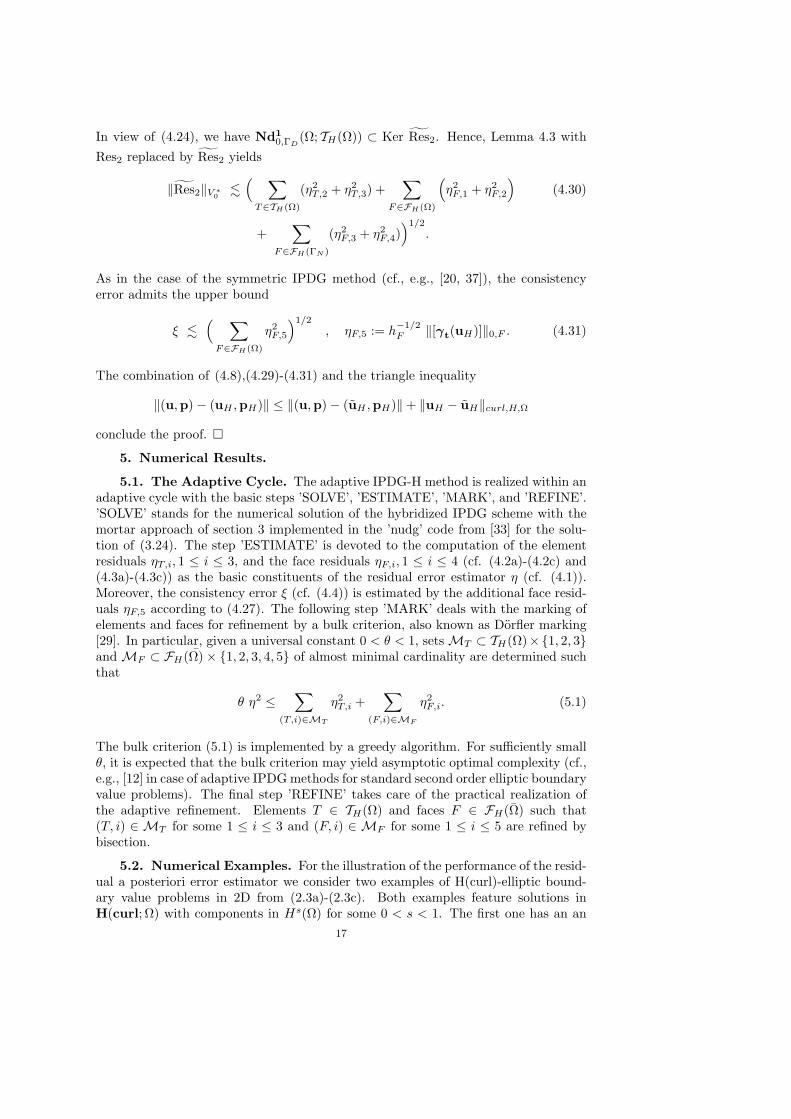
irrotational solution on an L-shaped domain with a singularity at the reentrant cornerand the second one exhibits a solenoidal solution on a circle with a cut out wedgehaving a singularity at the origin. For both problems, the penalty parameters in theIPDG-H method have been chosen according to α± := κ(k + 1)2/2 with κ = 100.

Example 1: We consider the L-shaped domain Ω := (−1, +1)2 \ [0,+1]× [−1, 0] withDirichlet boundary ΓD := (0× (0, 1) ∪ (0, 1)× 0), Neumann boundary ΓN := Γ \ ΓD

and data µ = σ = 1. The right-hand sides f , g1, g2 in (2.3a)-(2.3c) are chosen suchthat

u = grad(r2/3 sin(23ϕ))

is the exact solution (in polar coordinates). The solution is in H(curl; Ω)∩H2/3−ε(Ω)for any ε > 0 and exhibits a singularity at the reentrant corner.

−1 −0.5 0 0.5 1

−1

−0.5

0

0.5

1

Mesh Level 0

−1 −0.5 0 0.5 1

−1

−0.5

0

0.5

1

Mesh Level 8

−1 −0.5 0 0.5 1

−1

−0.5

0

0.5

1

Mesh Level 18

Fig. 5.1. Ex. 1: The initial mesh (left) and the meshes after 8 (middle) and 18 (right) adaptiverefinement steps (k = 4 and Θ = 0.1).

2 2.5 3 3.5 4 4.5 5−3.5

−3

−2.5

−2

−1.5

−1

−0.5

log DOF

log(

||(u

, p)

− (

u H ,

p H)|

| )

k=1

θ=0.1θ=0.3θ= 0.5θ =0.7uniform

2 2.5 3 3.5 4 4.5 5−3.5

−3

−2.5

−2

−1.5

−1

−0.5

log DOF

log(

||(u

, p)

− (

u H ,

p H)|

| )

k = 4

θ=0.1θ=0.3θ= 0.5θ =0.7uniform

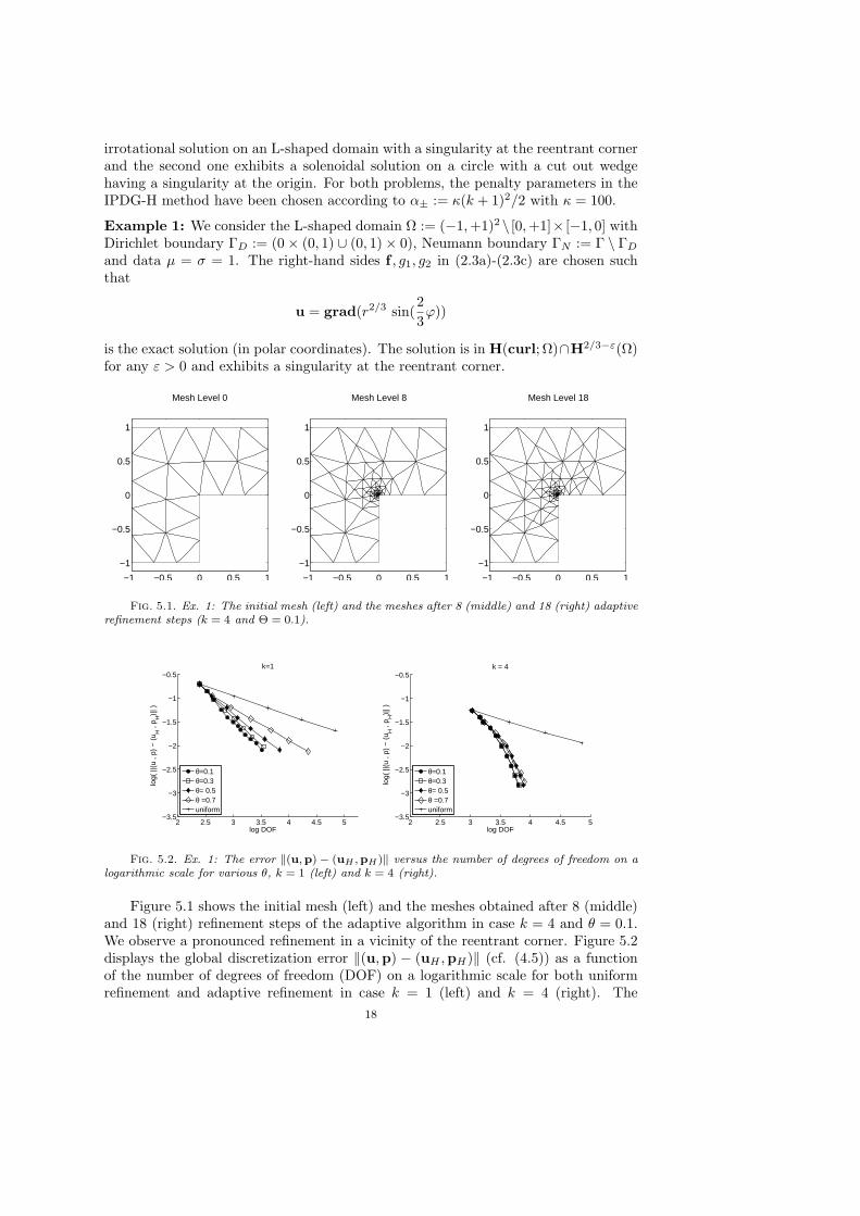
Fig. 5.2. Ex. 1: The error ‖(u,p)− (uH ,pH)‖ versus the number of degrees of freedom on alogarithmic scale for various θ, k = 1 (left) and k = 4 (right).

Figure 5.1 shows the initial mesh (left) and the meshes obtained after 8 (middle)and 18 (right) refinement steps of the adaptive algorithm in case k = 4 and θ = 0.1.We observe a pronounced refinement in a vicinity of the reentrant corner. Figure 5.2displays the global discretization error ‖(u,p) − (uH ,pH)‖ (cf. (4.5)) as a functionof the number of degrees of freedom (DOF) on a logarithmic scale for both uniformrefinement and adaptive refinement in case k = 1 (left) and k = 4 (right). The

18

results of the adaptive refinement are shown for various values of the constant θ inthe bulk criterion (5.1). Both for k = 1 and k = 4 the benefits of adaptive versusuniform refinement can be clearly seen. In case k = 1, we observe a dependence ofthe convergence rate on the parameter θ which is much less pronounced in case k = 4.According to the theory for IPDG methods applied to standard second order ellipticboundary value problems (cf. [12] and the numerical results in [34]), we see thatoptimality is asymptotically achieved for small θ.

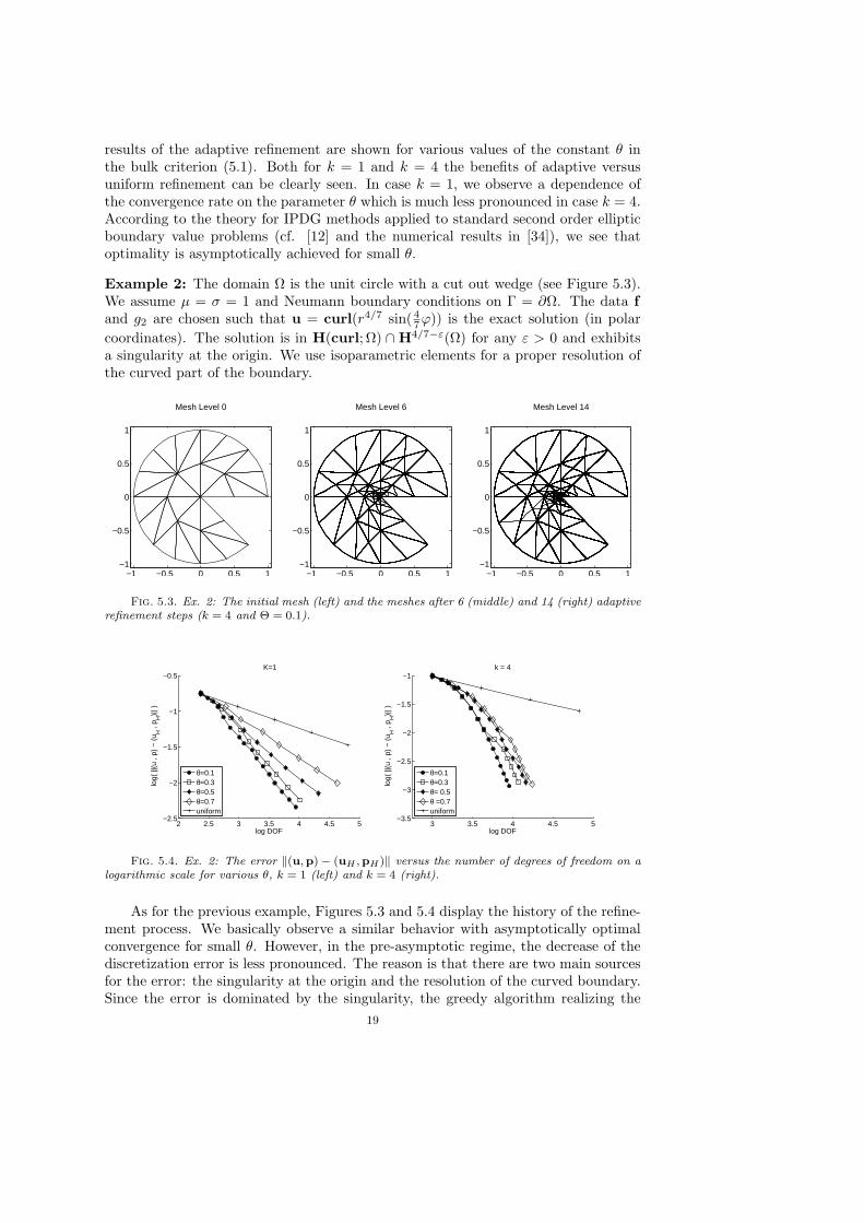
Example 2: The domain Ω is the unit circle with a cut out wedge (see Figure 5.3).We assume µ = σ = 1 and Neumann boundary conditions on Γ = ∂Ω. The data fand g2 are chosen such that u = curl(r4/7 sin( 4

7ϕ)) is the exact solution (in polarcoordinates). The solution is in H(curl; Ω) ∩H4/7−ε(Ω) for any ε > 0 and exhibitsa singularity at the origin. We use isoparametric elements for a proper resolution ofthe curved part of the boundary.

−1 −0.5 0 0.5 1−1

−0.5

0

0.5

1

Mesh Level 0

−1 −0.5 0 0.5 1−1

−0.5

0

0.5

1

Mesh Level 6

−1 −0.5 0 0.5 1−1

−0.5

0

0.5

1

Mesh Level 14

Fig. 5.3. Ex. 2: The initial mesh (left) and the meshes after 6 (middle) and 14 (right) adaptiverefinement steps (k = 4 and Θ = 0.1).

2 2.5 3 3.5 4 4.5 5−2.5

−2

−1.5

−1

−0.5

log DOF

log(

||(u

, p)

− (

u H ,

p H)|

| )

K=1

θ=0.1θ=0.3θ=0.5θ=0.7uniform

3 3.5 4 4.5 5−3.5

−3

−2.5

−2

−1.5

−1

log DOF

log(

||(u

, p)

− (

u H ,

p H)|

| )

k = 4

θ=0.1θ=0.3θ= 0.5θ =0.7uniform

Fig. 5.4. Ex. 2: The error ‖(u,p)− (uH ,pH)‖ versus the number of degrees of freedom on alogarithmic scale for various θ, k = 1 (left) and k = 4 (right).

As for the previous example, Figures 5.3 and 5.4 display the history of the refine-ment process. We basically observe a similar behavior with asymptotically optimalconvergence for small θ. However, in the pre-asymptotic regime, the decrease of thediscretization error is less pronounced. The reason is that there are two main sourcesfor the error: the singularity at the origin and the resolution of the curved boundary.Since the error is dominated by the singularity, the greedy algorithm realizing the

19

bulk criterion (5.1) picks the corresponding residuals first until those associated withthe boundary resolution are taken into account.

REFERENCES

[1] M. Ainsworth, A posteriori error estimation for Discontinuous Galerkin finite element approx-imation. SIAM J. Numer. Anal. 45, 1777–1798, 2007.

[2] M. Ainsworth and T. Oden, A Posteriori Error Estimation in Finite Element Analysis. Wiley,Chichester, 2000.

[3] D.N. Arnold, An interior penalty finite element method with discontinuous elements. SIAM J.Numer. Anal. 19, 742–760, 1982.

[4] D.N. Arnold and F. Brezzi, Mixed and nonconforming finite element methods: implementation,postprocessing and error estimates. RAIRO Model. Math. Anal. Numer. 19, 7–32, 1985.

[5] D.N. Arnold, F. Brezzi, B. Cockburn, and D. Marini, Unified analysis of discontinuous Galerkinmethods for elliptic problems. SIAM J. Numer. Anal. 39, 1749–1779, 2002.

[6] I. Babuska and T. Strouboulis, The Finite Element Method and its Reliability. Clarendon Press,Oxford, 2001.

[7] W. Bangerth and R. Rannacher, Adaptive Finite Element Methods for Differential Equations.Lectures in Mathematics. ETH-Zurich. Birkhauser, Basel, 2003.

[8] R. Beck, P. Deuflhard, R. Hiptmair, R.H.W. Hoppe, and B. Wohlmuth, Adaptive multilevelmethods for edge element discretizations of Maxwell’s equations. Surveys of Math. in In-dustry 8, 271–312, 1999.

[9] R. Beck, R. Hiptmair, R.H.W. Hoppe, and B. Wohlmuth, Residual based a posteriori error

estimators for eddy current computation. M2AN Math. Modeling and Numer. Anal. 34,159–182, 2000.

[10] R. Beck, R. Hiptmair, and B. Wohlmuth, Hierarchical error estimator for eddy current com-putation. In: Proc. 2nd European Conf. on Advanced Numer. Meth. (ENUMATH99),Jyvaskyla, Finland, July 26-30, 1999 (Neittaanmaki, P. et al.; eds.), pp. 111–120, WorldScientific, Singapore, 2000.

[11] R. Becker, P. Hansbo, and M.G. Larson, Energy norm a posteriori error estimation for discon-tinuous Galerkin methods. Comput. Methods Appl. Mech. Engrg. 192, 723–733, 2003.

[12] A. Bonito and R. Nochetto, Quasi-optimal convergence rate of an adaptive DiscontinuousGalerkin method. Preprint. Department of Mathematics, University of Maryland, 2008.

[13] J.H. Bramble and J. Xu, A local post-processing technique for improving the accuracy in mixedfinite element approximations. SIAM J. Numer. Anal. 26, 1267–1275, 1989.

[14] J. Brandts, Superconvergence and a posteriori error estimation for triangular mixed finiteelement methods. Numer. Math. 68, 311–324, 1994.

[15] F. Brezzi, J. Douglas, Jr., and L.D. Marini, Two families of mixed finite elements for secondorder elliptic problems. Numer. Math. 47, 217–235, 1985.

[16] A. Buffa, M. Costabel, and D. Sheen, On traces for H(curl, Ω) in Lipschitz domains, J. Math.Anal. Appl. 276, 845–867, 2002.

[17] C. Carstensen, A unifying theory of a posteriori finite element error control. Numer. Math.100, 617–637, 2005.

[18] C. Carstensen, T. Gudi, and M. Jensen, A unifying theory of a posteriori error control fordiscontinuous Galerkin FEM. Numer. Math. 112, 363–379, 2009.

[19] C. Carstensen and R.H.W. Hoppe, Convergence analysis of an adaptive edge finite elementmethod for the 2d eddy current equations. J. Numer. Math. 13, 19–32, 2005.

[20] C. Carstensen and R.H.W. Hoppe, Unified framework for an a posteriori error analysis of non-standard finite element approximations of H(curl)-elliptic problems. J. Numer. Math. 17,27–44, 2009.

[21] C. Carstensen and J. Hu, A unifying theory of a posteriori error control for nonconformingfinite element methods. Numer. Math. 107, 473–502, 2007.

[22] C. Carstensen, J. Hu, and A. Orlando, Framework for the a posteriori error analysis of non-conforming finite elements. SIAM J. Numer. Anal. 45, 68–82, 2007.

[23] P. Castillo, B. Cockburn, I. Perugia, and D. Schotzau, An a priori error estimate of the localdiscontinuous Galerkin method for elliptic problems. SIAM J. Numer. Anal. 38, 1676–1706,2000.

[24] B. Cockburn, Discontinuous Galerkin methods. Z. Angew. Math. Mech. 83, 731–754, 2003.

20

[25] Cockburn, B., and Gopalakrishnan, J.; A characterization of hybridized mixed methods forsecond order elliptic problems. SIAM J. Numer. Anal. 42, 283–301, 2004.

[26] Cockburn, B., and Gopalakrishnan, J.; Error analysis of variable degree mixed methods forelliptic problems via hybridization. Math. Comp. 74, 1653–1677, 2005.

[27] Cockburn, B., and Gopalakrishnan, J.; New hybridization techniques. GAMM-Mitteilungen 2,154–183 (2005).

[28] Cockburn, B., Gopalakrishnan, J., and Lazarov, R.; Unified hybridization of discontinuousGalerkin, Mixed and continuous Galerkin methods for second order elliptic problems. SIAMJ. Numer. Anal. 47, 1319–1365, 2009.

[29] Dorfler, W.; A convergent adaptive algorithm for Poisson’s equation. SIAM J. Numer. Anal.33, 1106–1124, 1996.

[30] K. Eriksson, D. Estep, P. Hansbo, and C. Johnson, Computational Differential Equations.Cambridge University Press, Cambridge, 1996.

[31] B.M. Fraejis de Veubeke, Displacement and equilibrium methods in the finite element method.In: Stress Analysis (O. Zienkiewicz and G. Hollister; eds.), pp. 145–197, Wiley, New York,1977.

[32] V. Girault and P.A. Raviart, Finite Element Approximatiuon of the Navier-Stokes Equations.Lecture Notes in Mathematics 749, Springer, Berlin-Heidelberg-New York, 1979.

[33] J.S. Hesthaven and T. Warburton, Nodal Discontinuous Galerkin Methods. Springer, Berlin-Heidelberg-New York, 2008.

[34] R.H.W. Hoppe, G. Kanschat, and T. Warburton, Convergence analysis of an adaptive interiorpenalty discontinuous Galerkin method. SIAM J. Numer. Anal., 47, 534–550, 2009.

[35] R.H.W. Hoppe and J. Schoberl, Convergence of adaptive edge element methods for the 3Deddy currents equations. J. Comp. Math. 27, 657–676, 2009.

[36] P. Houston, I. Perugia, and D. Schotzau, Mixed discontinuous Galerkin approximation of theMaxwell operator. SIAM J. Numer. Anal. 42, 434–459, 2004.

[37] P. Houston, I. Perugia, and D. Schotzau, A posteriori error estimation for discontinuousGalerkin discretizations of H(curl)-elliptic partial differential equations. IMA Journal ofNumerical Analysis 27, 122–150, 2007.

[38] P. Houston, D. Schotzau, and T.P. Wihler, Energy norm a posteriori error estimation of hp-adaptive discontinuous Galerkin methods for elliptic problems. Math. Models MethodsAppl. Sci. 17, 33–62, 2007.

[39] G. Kanschat and R. Rannacher, Local error analysis of the interior penalty discontinuousGalerkin method for second order problems. J. Numer. Math. 10, 249–274, 2002.

[40] O. Karakashian and F. Pascal, A posteriori error estimates for a discontinuous Galerkin ap-proximation of second-order elliptic problems. SIAM J. Numer. Anal. 41, 2374–2399, 2003.

[41] O. Karakashian and F. Pascal, Convergence of adaptive Doiscontinuous Galerkin approxima-tions of second-order elliptic problems. SIAM J. Numer. Anal. 45, 641–665, 2007.

[42] P. Monk, Finite Element Methods for Maxwell’s equations, Clarendon Press, Oxford, 2003.[43] J.C. Nedelec, Mixed finite elements in R3, Numer. Math. 35, 315–341, 1980.[44] P. Neittaanmaki and S. Repin, Reliable methods for mathematical modelling. Error control

and a posteriori estimates. Elsevier, New York, 2004.[45] S. Nicaise and E. Creuse, Isotropic and anisotropic a posteriori error estimation of the mixed

finite element method for second order operators in divergence form. ETNA 23, 38–62,2006.

[46] I. Perugia, D. Schotzau, and P. Monk, Stabilized interior penalty methods for the time-harmonicMaxwell equations. Comp. Meth. Appl. Mech. Engrg. 191, 4675–4697, 2002.

[47] B. Riviere and M.F. Wheeler, A posteriori error estimates and mesh adaptation strategy fordiscontinuous Galerkin methods applied to diffusion problems. Computers & Mathematicswith Applications 46, 141–163, 2003.

[48] J. Schoberl, A posteriori error estimates for Maxwell equations, Math. Comp. 77, 633–649,2008.

[49] R. Verfurth, A Review of A Posteriori Estimation and Adaptive Mesh-Refinement Techniques.Wiley-Teubner, New York, Stuttgart, 1996.

[50] B. Wohlmuth and R.H.W. Hoppe, A comparison of a posteriori error estimators for mixed finiteelement discretizations. Math. Comp. 82, 253–279, 1999.

[51] X. Xu and R.H.W. Hoppe, On the convergence of mortar edge element methods in R3. SIAMJ. Numer. Anal. 43, 1276–1294, 2005.

21