Embed Size (px)
Citation preview

ADAPTIVE IMAGE QUALITY IMPROVEMENT
WITH BAYESIAN CLASSIFICATION FOR IN-LINE MONITORING
By
Shuo Yan
A thesis submitted in conformity with the requirements
for the degree of Doctor of Philosophy
Graduate Department of Chemical Engineering and Applied Chemistry
University of Toronto
© Copyright by Shuo Yan 2008

ii
ADAPTIVE IMAGE QUALITY IMPROVEMENT
WITH BAYESIAN CLASSIFICATION
FOR IN-LINE MONITORING
Shuo Yan
Doctor of Philosophy
Department of Chemical Engineering and Applied Chemistry
University of Toronto
2008
ABSTRACT
Development of an automated method for classifying digital images using a combination
of image quality modification and Bayesian classification is the subject of this thesis.
The specific example is classification of images obtained by monitoring molten plastic in
an extruder. These images were to be classified into two groups: the “with particle”
(WP) group which showed contaminant particles and the “without particle” (WO) group
which did not. Previous work effected the classification using only an adaptive Bayesian
model. This work combines adaptive image quality modification with the adaptive
Bayesian model. The first objective was to develop an off-line automated method for
determining how to modify each individual raw image to obtain the quality required for
improved classification results. This was done in a very novel way by defining image
iii
quality in terms of probability using a Bayesian classification model. The Nelder Mead
Simplex method was then used to optimize the quality. The result was a “Reference
Image Database” which was used as a basis for accomplishing the second objective. The
second objective was to develop an in-line method for modifying the quality of new
images to improve classification over that which could be obtained previously. Case
Based Reasoning used the Reference Image Database to locate reference images similar
to each new image. The database supplied instructions on how to modify the new image
to obtain a better quality image. Experimental verification of the method used a variety
of images from the extruder monitor including images purposefully produced to be of
wide diversity. Image quality modification was made adaptive by adding new images to
the Reference Image Database. When combined with adaptive classification previously
employed, error rates decreased from about 10% to less than 1% for most images. For
one unusually difficult set of images that exhibited very low local contrast of particles in
the image against their background it was necessary to split the Reference Image
Database into two parts on the basis of a critical value for local contrast. The end result
of this work is a very powerful, flexible and general method for improving classification
of digital images that utilizes both image quality modification and classification
modeling.

iv
ACKNOWLEDGMENT I would like to express my gratitude to all those who made this research an enjoyable and
exciting journey.
First, my deepest gratitude goes to Professor Stephen T. Balke for his persistent guidance,
continuous encouragement, and patience during this research. His committed supervision
and unreserved support are greatly appreciated.
Next, I am very much indebted to Dr. Saed Sayad for his invaluable guidance and
participation in this project. In particular, I am very grateful for his excellent advice
regarding applying data mining techniques, as well as his assistance in improving the
programming involved in this research.
I would also like to acknowledge my Ph.D. committee members for their important
guidance and constructive comments throughout the research: Professor G. J. Evans,
Professor M. T. Kortschot, and Professor R. Mahadevan. In addition, I thank my fellow
students who helped me with my research: Dr. Keivan Torabi, Ms. Forouz Farahani, and
all of my other friends in the Department of Chemical Engineering and Applied
Chemistry.
Finally, I would like to express my deepest gratitude for the constant encouragement and
support of my parents, Guangguo Tan and Xiufang Wei, and of my very patient wife,
Yingjing Fu, during these many years of intensive work.
v
TABLE OF CONTENTS ABSTRACT ................................................................................................................................................. II ACKNOWLEDGMENT............................................................................................................................ IV TABLE OF CONTENTS.............................................................................................................................V LIST OF TABLES.................................................................................................................................... VII LIST OF FIGURES......................................................................................................................................X NOMENCLATURE ................................................................................................................................XIII 1 INTRODUCTION............................................................................................................................... 1 2 LITERATURE REVIEW AND STRATEGY DEVELOPMENT.................................................. 4
2.1 IN-LINE IMAGE MONITORING ....................................................................................................... 4 2.2 CLASSIFICATION METHODS.......................................................................................................... 6
2.2.1 Overview of Classification...................................................................................................... 6 2.2.2 The Torabi Bayesian Classification Model............................................................................. 7
2.2.2.1 Thresholding ................................................................................................................................ 7 2.2.2.2 Bayesian Classification ................................................................................................................ 9
2.3 OFF-LINE IMAGE QUALITY MODIFICATION ................................................................................ 18 2.3.1 Proposed Strategy for Accomplishing the First Objective.................................................... 18 2.3.2 Defining Image Quality: Image Quality Metrics ................................................................. 19 2.3.3 Image Quality Operators (IQ Operators)............................................................................. 22 2.3.4 Optimizing Image Quality..................................................................................................... 24
2.4 IN-LINE IMAGE QUALITY MODIFICATION................................................................................... 25 2.4.1 Proposed Strategy for Accomplishing the Second Objective................................................ 25 2.4.2 Use of the Reference Image Database: Case-based Reasoning ........................................... 26
2.4.2.1 Advantages of Case-Based Reasoning ....................................................................................... 28 2.4.2.2 Case-Based Reasoning in Image Interpretation.......................................................................... 29 2.4.2.3 The Case-Based Reasoning Process........................................................................................... 30 2.4.2.4 Case Retrieval in Image Interpretation....................................................................................... 33 2.4.2.5 Case Retention in Case Based Reasoning .................................................................................. 36 2.4.2.6 Computation Efficiency of Case-Based Reasoning.................................................................... 37
2.5 EVALUATION OF CLASSIFICATION METHODS............................................................................. 39 3 EXPERIMENTAL PROCEDURE.................................................................................................. 46 4 COMPUTATIONAL PROCEDURE.............................................................................................. 49
4.1 SOFTWARE DEVELOPMENT FOR THE FIRST OBJECTIVE: OFF-LINE IMAGE QUALITY MODIFICATION ......................................................................................................................................... 49
4.1.1 The Simplex Optimization Component ................................................................................. 51 4.1.2 The Image Processing Shared Component ........................................................................... 53 4.1.3 The Image Measurement Shared Component ....................................................................... 54 4.1.4 The Image Thresholding Shared Component ....................................................................... 56 4.1.5 The Image Classification Shared Component....................................................................... 57 4.1.6 The Database Shared Component ........................................................................................ 58
4.2 SOFTWARE DEVELOPMENT FOR THE SECOND OBJECTIVE: IN-LINE IMAGE QUALITY MODIFICATION ......................................................................................................................................... 61
5 RESULTS AND DISCUSSION ....................................................................................................... 65 5.1 OFF-LINE IMAGE MODIFICATION................................................................................................ 65
5.1.1 Selection of Image Quality Operators and their Order of Application................................. 69 5.1.1.1 Screen 1: Constraining Selection of IQ Operators by Selecting the Image Analysis Software . 69 5.1.1.2 Screen 2: Selection of IQ Operators by Image Characteristics................................................. 71 5.1.1.3 The Application of Screen 2 to Images Obtained by the Scanning Particle Monitor ................. 75 5.1.1.4 Screen 3: Dimensionality Reduction: Selection of IQ Operators by Task Specific Criteria...... 78

vi
5.1.2 Image Quality Definition ...................................................................................................... 80 5.1.2.1 Least Squares as Objective Function.......................................................................................... 81 5.1.2.2 Weighted Least Squares (WLS) as Objective Function ............................................................. 89 5.1.2.3 The Desirability Function as Objective Function....................................................................... 96 5.1.2.4 Probability Density Difference as Objective Function............................................................. 100
5.1.3 Comparison of Classification Results for Different Objective Functions........................... 108 5.2 IN-LINE IMAGE QUALITY MODIFICATION................................................................................. 113
5.2.1 The Reference Image Database .......................................................................................... 113 5.2.2 In-line Image Quality Modification for Classification: Use of a Static Classification Model 116 5.2.3 In-line Adaptive Image Quality Modification with Adaptive Classification ....................... 122
5.2.3.1 Test Trial 1: the Use of a New Set of Images Produced by Torabi ......................................... 124 5.2.3.2 Test Trial 2: the Use of Microgel Image Set Produced by Ing ................................................ 126 5.2.3.3 Test Trial 3: the Use of Images from New Extruder Runs Utilizing Injection of Particles with Low Additive Polyethylene Pelletized Feed ................................................................................................. 129 5.2.3.4 Test Trial 4: the Use of Images from New Extrusion Runs Utilizing Injection of Particles with High Additive Polyethylene Pelletized Feed................................................................................................. 131 5.2.3.5 The Application of Decision Rule in Case-based Reasoning (CBR)........................................ 134 5.2.3.6 Classification Results after the Application of Decision Rule in Case-Based Reasoning ........ 136
5.2.4 Summary of the Method Developed for the Second Objective............................................ 140 6 CONCLUSIONS ............................................................................................................................. 142 7 RECOMENDATIONS ................................................................................................................... 144 8 APPENDICES................................................................................................................................. 145
APPENDIX I AN OVERVIEW OF OBJECTIVE IMAGE QUALITY METRICS (IQ METRICS)........................ 145 APPENDIX II IMAGE QUALITY OPERATORS .................................................................................... 159
Radiometric Operators .................................................................................................................................. 159 Arithmetic-based operations ......................................................................................................................... 167 Geometric Operators ..................................................................................................................................... 167 Mathematical Morphological Operators........................................................................................................ 176 Non-uniform Illumination Correction ........................................................................................................... 179
APPENDIX III THE NELDER-MEAD SIMPLEX METHOD..................................................................... 180 Basic Simplex Method .................................................................................................................................. 180 Modified Simplex Method (Nelder-Mead) ................................................................................................... 182 Transformation of Constraints in the Utilization of Simplex Optimization................................................... 184 Simplex Optimization Stopping Criteria ....................................................................................................... 185 Objective Function........................................................................................................................................ 186 Other Considerations on the Utilization of Simplex Method ........................................................................ 187
APPENDIX IV MODIFIED MAXMIN THRESHOLDING......................................................................... 188 APPENDIX V ADAPTIVE MACHINE LEARNING METHODS .................................................. 197
The Intelligent Learning Machine (ILM) ...................................................................................................... 197 Incremental Support Vector Machine (ISVM).............................................................................................. 203 Incremental Neural Networks (INN)............................................................................................................. 205
APPENDIX VI SCREEN 3: SELECTION OF IQ OPERATORS BY TASK SPECIFIC CRITERIA ................... 208 Screen 3: Trial 1............................................................................................................................................ 209 Screen 3: Trial 2............................................................................................................................................ 214 Screen 3: Trial 3............................................................................................................................................ 215 Screen 3: Trial 4............................................................................................................................................ 217
APPENDIX VII CASE-BASED REASONING CLASSIFICATION............................................................... 219 APPENDIX VIII COMPUTATION TIME FOR DIFFERENT CLASSIFICATION METHODS........................ 228 APPENDIX IX STATISTICS ON THE ESTIMATION OF PROPORTIONS.................................................... 229
9 REFERENCES................................................................................................................................ 235

vii
LIST OF TABLES Table 2-1 Confusion Matrix for a Binary Classification Problem.................................... 40 Table 2-2 Confusion Matrix for a Binary Classification Problem Showing Data Mining Measures ........................................................................................................................... 40 Table 2-3 Definition of Terms Related to Classification.................................................. 41 Table 3-1 Summary of Image Data Sets Used in This Work ........................................... 47 Table 3-2 Image Data Sets Produced from Experimental Extrusion Runs in this Research........................................................................................................................................... 48 Table 5-1 Image Quality Operators .................................................................................. 71 Table 5-2 Classification Confusion Matrix for the Training Set of Raw Images............. 83 Table 5-3 Classification Confusion Matrix for the Training Set of Images Optimized Using the Least Squares Objective Function .................................................................... 83 Table 5-4 Relationship between Least Squares as Objection Function and Classification Accuracy ........................................................................................................................... 87 Table 5-5 Image Quality Distribution for Least Squares Optimized Images ................... 88 Table 5-6 Weight Factors for Weighted Least Squares Image Quality Definition........... 90 Table 5-7 Confusion Matrix for Weighted Least Squares Optimized Images.................. 91 Table 5-8 Comparison of AUC for Least Squares and Weighted Least Squares Optimized Images ............................................................................................................................... 93 Table 5-9 Relationship between Weighted Least Squares as Objection Function and Classification Accuracy .................................................................................................... 94 Table 5-10 Image Quality Distribution for Weight Least Squares Optimized Images..... 95 Table 5-11 Confusion Matrix for Desirability Function Optimized Images .................... 97 Table 5-12 Image Quality Distribution of Desirability Function Optimized Images....... 99 Table 5-13 Parameter Values in Classification Models.................................................. 105 Table 5-14 Confusion Matrix for Training Image Set Using Probability Density Difference as Objective Function ................................................................................... 106 Table 5-15 Comparison of AUC among Different Objective Functions........................ 111 Table 5-16 Image Quality Metrics for the Training Image Set After Blanket Processing......................................................................................................................................... 111 Table 5-17 A Portion of Reference Image Database ...................................................... 114 Table 5-18 Similarity Attributes ..................................................................................... 117 Table 5-19 Confusion Matrix for a Subset of Image Set 1 Using IQMod Classification120 Table 5-20 Confusion Matrix for a Subset of Image Set 1 Using Bayesian Classification......................................................................................................................................... 121 Table 5-21 Confusion Matrix of Test Trial 1 Image Set Using In-line Adaptive Bayesian Classification................................................................................................................... 124 Table 5-22 Confusion Matrix of Test Trial 1 Image Set Using Static IQMod Classification................................................................................................................... 124 Table 5-23 Confusion Matrix of Test Trial 1 Image Set Using Adaptive IQMod Classification................................................................................................................... 125 Table 5-24 Image Quality Metrics of Test Trial 2 Microgel Image Set ......................... 127

viii
Table 5-25 Confusion Matrix of Test Trial 2 Image Set Using In-line Adaptive Classification................................................................................................................... 127 Table 5-26 Confusion Matrix of Test Trial 2 Image Set Using Static IQMod Classification................................................................................................................... 127 Table 5-27 Confusion Matrix of Test Trial 2 Image Set Using Adaptive IQMod Classification................................................................................................................... 127 Table 5-28 Image Quality Metrics of Test Trial 3 Image Set......................................... 129 Table 5-29 Confusion Matrix for Test Trial 3 Image Subset (Run 3-1 in Table 3-2) Using Adaptive IQMod Classification ...................................................................................... 130 Table 5-30 Confusion Matrix for Test Trial 3 Image Subset (Run 3-2 in Table 3-2) Using Adaptive IQMod Classification ...................................................................................... 130 Table 5-31 Confusion Matrix for Test Trial 3 Image Subset (Run 3-3 in Table 3-2) Using Adaptive IQMod Classification ...................................................................................... 130 Table 5-32 Confusion Matrix for Trial 3 Image Subset (Run 3-4 in Table 3-2) Using Adaptive IQMod Classification ...................................................................................... 130 Table 5-33 Confusion Matrix for Test Trial 4 Batch-A Image Set (Run 3-5 in Table 3-2) Using Adaptive IQMod Classification............................................................................ 132 Table 5-34 Confusion Matrix for Test Trial 4 Batch-A Image Set (Run 3-6 in Table 3-2) Using Adaptive IQMod Classification............................................................................ 132 Table 5-35 Image Quality Metrics for Test Trial 4 Image Set ....................................... 133 Table 5-36 The Effect of Local Contrast Threshold on Classification Error Rate for Test Trial 4.............................................................................................................................. 137 Table 5-37 Confusion Matrix of Test Trial 4 Using Adaptive IQMod Classification with Decision Rule.................................................................................................................. 139 Table 5-38 Confusion Matrix of Test Trial 4 Using In-line Adaptive Bayesian Classification................................................................................................................... 139 Table 8-1 Two-way ANOVA Table for Quantifying the Illumination Uniformity........ 156 Table 8-2 Comparison of Illumination Uniformity for Raw Images and Their Illumination Corrected Images ............................................................................................................ 158 Table 8-3 Threshold Test of Modified MaxMin Thresholding ...................................... 194 Table 8-4 Classification Confusion Matrix for MaxMin Thresholding.......................... 195 Table 8-5 Classification Confusion Matrix for Modified MaxMin Thresholding.......... 195 Table 8-6 The General Structure of ILM Weight Table ................................................. 198 Table 8-7 The Basic Unit of the ILM Weight Table ...................................................... 198 Table 8-8 ILM Knowledge Table for N images.............................................................. 201 Table 8-9 Statistical Experimental Designs.................................................................... 209 Table 8-10 Two Level Factorial Design for an Image Operator Sequence .................... 211 Table 8-11 Confusion Matrix of Test Trial 1 Image Set Using CBR Classification...... 221 Table 8-12 Confusion Matrix of Test Trial 2 Image Set Using CBR Classification...... 222 Table 8-13 Confusion Matrix for Test Trial 3 Image Subset (Run 3-1 to Run 3-4 in Table 3-2) Using Torabi Adaptive Classification ..................................................................... 224 Table 8-14 Confusion Matrix for Test Trial 3 Image Subset (Run 3-1 to Run 3-4 in Table 3-2) Using CBR Classification ....................................................................................... 224 Table 8-15 Confusion Matrix for Test Trial 3 Image Subset (Run 3-1 to Run 3-4 in Table 3-2) Using Static IQMod Classification ......................................................................... 224

ix
Table 8-16 Confusion Matrix for Test Trial 3 Image Subset (Run 3-1 to Run 3-4 in Table 3-2) Using Adaptive IQMod Classification.................................................................... 224 Table 8-17 Confusion Matrix for Test Trial 4 Batch-A Image Set (Run 3-6 in Table 3-2) Using Torabi Adaptive Classification............................................................................. 226 Table 8-18 Confusion Matrix for Test Trial 4 Batch-A Image Set (Run 3-6 in Table 3-2) Using CBR Classification ............................................................................................... 226 Table 8-19 Confusion Matrix for Test Trial 4 Batch-A Image Set (Run 3-6 in Table 3-2) Using Static IQMod Classification ................................................................................. 226 Table 8-20 Confusion Matrix for Test Trial 4 Batch-A Image Set (Run 3-6 in Table 3-2) Using Adaptive IQMod Classification............................................................................ 226 Table 8-21 Computation Time for Different Classification Methods ............................ 228 Table 8-22 Errors from 10-Fold Cross Validation for Classification Models Created Based on Images Optimized Using Different Image Quality Definitions ...................... 229 Table 8-23 A Sample Classification Confusion Matrix.................................................. 232

x
LIST OF FIGURES Figure 2-1 Torabi Bayesian Classification Method .......................................................... 10 Figure 2-2 Mircogel image with no additive in the background ...................................... 14 Figure 2-3 Glass Microsphere (GMS) Images with talc additive in the background ...... 15 Figure 2-4 Incremental Adaptation of Bayesian Classification Model ............................ 16 Figure 2-5 Case-Based Reasoning Process....................................................................... 32 Figure 2-6 Example of a Receiver Operating Characteristic (ROC) Curve ..................... 44 Figure 3-1 In-Line Image Monitoring System for Plastics Film Extrusion...................... 46 Figure 4-1 Computational Software Components Associated with Off-line Image Quality Modification...................................................................................................................... 50 Figure 4-2 Simplex Optimization Component in Off-line Image Quality Modification. 52 Figure 4-3 Image Processing Shared Component............................................................. 53 Figure 4-4 Image Measurement Shared Component ........................................................ 55 Figure 4-5 Image Thresholding Shared Component......................................................... 57 Figure 4-6 Functionalities of Image Classification Shared Components ......................... 59 Figure 4-7 Reference Image Database Shared Components............................................. 60 Figure 4-8 Computational Software Components Associated with In-line Image Quality Modification...................................................................................................................... 62 Figure 4-9 Case-based Reasoning Component in In-line Image Quality Modification ... 64 Figure 5-1 Off-line Image Quality Modification Framework........................................... 68 Figure 5-2 Layered Screening of IQ Operators ............................................................... 70 Figure 5-3 Pre-selection of Image Operators for Noise Removal .................................... 73 Figure 5-4 Pre-selection of Image Operators for Blur Removal....................................... 73 Figure 5-5 Pre-selection of Image Operators for Contrast Enhancement......................... 73 Figure 5-6 Pre-selection of Image Operators for Illumination Correction ....................... 74 Figure 5-7 Pre-selection of Image Operators for Brightness Adjustment ........................ 74 Figure 5-8 Example Real Image 1 .................................................................................... 76 Figure 5-9 Example Real Image 2 .................................................................................... 77 Figure 5-10 Classification Error Rate for Least Squares as Objective Function.............. 84 Figure 5-11 ROC Curve for Least Squares as Objective Function................................... 85 Figure 5-12 Image Quality Distribution for Least Squares Optimized Images ................ 88 Figure 5-13 Image Quality Histogram for Least Squares Optimized Images .................. 89 Figure 5-14 Classification Error Rates for Weighted Least Squares Optimized Images . 92 Figure 5-15 ROC Curve for Weighted Least Squares Optimized Images........................ 93 Figure 5-16 Image Quality Distribution for Weighted Least Squares Optimized Images 95 Figure 5-17 Image Quality Histogram for Weighted Least Squares Optimized Images.. 96 Figure 5-18 Classification Error Rate for Desirability Function Optimized Images........ 98 Figure 5-19 ROC Curve for Desirability Function Optimized Images............................. 98 Figure 5-20 Image Quality Distribution of Desirability Function Optimized Images...... 99 Figure 5-21 Image Quality Histogram for Desirability Function Optimized Images..... 100 Figure 5-22 Classification Error Rate for Probability Density Difference Optimized Images ............................................................................................................................. 107 Figure 5-23 ROC Curve for Probability Density Difference Optimized Images ........... 108
xi
Figure 5-24 Comparison of Classification Error Rates among Different Objective Functions......................................................................................................................... 109 Figure 5-25 Comparison of False Negative Rates among Different Objective Functions......................................................................................................................................... 110 Figure 5-26 Comparison of False Positive Rates among Different Objective Functions110 Figure 5-27 ROC Analysis of the Classification Performance of Different Objective Functions......................................................................................................................... 111 Figure 5-28 In-line Image Quality Modification Framework........................................ 119 Figure 5-29 Comparison of Classification Error Rates between Bayesian Classification and IQMod Classification ............................................................................................... 121 Figure 5-30 Comparison of Classification Error Rates for Test Trial 1 among Different Models............................................................................................................................. 126 Figure 5-31 Comparison of Classification Error Rates for Test Trial 2 among Different Models............................................................................................................................. 128 Figure 5-32 Classification Error Rates for Test Trial 3 Using Adaptive IQMod Classification................................................................................................................... 131 Figure 5-33 Classification Results for Test Trial 4 Image Set Using Adaptive IQMod Classification................................................................................................................... 133 Figure 5-34 The Application of Decision Rule in Case-Based Reasoning..................... 135 Figure 5-35 The Effect of Local Contrast Threshold on Classification Error Rate for Test Trial 4.............................................................................................................................. 137 Figure 5-36 The Effect of Local Contrast Threshold on Classification Accuracy for Test Trial 4.............................................................................................................................. 138 Figure 5-37 Comparison for Classification Error Rates for Test Trial 4 among Different Models............................................................................................................................. 139 Figure 8-1 Quantification of Illumination Uniformity Using ANOVA Analysis........... 155 Figure 8-2 Examples of Kernels ..................................................................................... 174 Figure 8-3 Normalized Gaussian kernel with σ =1.4...................................................... 175 Figure 8-4 Schematic Diagram of Basic Simplex Method ............................................. 183 Figure 8-5 Schematic Diagram of Modified Simplex Method ....................................... 183 Figure 8-6 Flow Chart of Modified Simplex Algorithm ................................................ 186 Figure 8-7 An Example Image........................................................................................ 191 Figure 8-8 The Effect of Thresholding Step Size on Minimum Particle Size ................ 191 Figure 8-9 Scheme of Modified Search for Threshold ................................................... 193 Figure 8-10 Comparison of Classification Error Rates for two Different Thresholding Methods........................................................................................................................... 196 Figure 8-11 ROC Curves for MaxMin Thresholding and Modified MaxMin Thresholding......................................................................................................................................... 196 Figure 8-12 The Intelligent Learning Machine (ILM).................................................... 197 Figure 8-13 Test Pattern Image 1................................................................................... 210 Figure 8-14 Graphical Illustration of the Execution of Two-Level Factorial Design on a Test Pattern ..................................................................................................................... 210 Figure 8-15 Plot of Two-Way Interaction Effect of Grayscale Erosion and Grayscale Dilation ........................................................................................................................... 212 Figure 8-16 Color-coded Scatterplot Matrix for Sequence of Grayscale dilation, Grayscale erosion and Median filter ............................................................................... 214
xii
Figure 8-17 Test Pattern Image 2.................................................................................... 215 Figure 8-18 Color-coded Scatterplot Matrix for Sequence of Median and Gaussian Filters......................................................................................................................................... 215 Figure 8-19 Test Pattern Image 3.................................................................................... 216 Figure 8-20 Color-coded Scatterplot Matrix for Sequence of Brightness shift, Median and Gaussian Filters............................................................................................................... 216 Figure 8-21 Test Pattern Image 4.................................................................................... 217 Figure 8-22 Color-coded Scatterplot Matrix for the Sequence of Brightness shift, Median filter, Gaussian Filter and the Unsharp Mask ................................................................. 218 Figure 8-23 The Schema of Case-Based Reasoning Classification................................ 220 Figure 8-24 The Case-Based Reasoning Classification Component .............................. 221 Figure 8-25 Comparison of Classification Error Rates for Test Trial 1 Using Different Classification Methods.................................................................................................... 222 Figure 8-26 Comparison of Classification Error Rates for Test Trial 2 Using Different Classification Methods.................................................................................................... 223 Figure 8-27 Classification Error Rates for Test Trial 3 Using Different Classification Methods........................................................................................................................... 225 Figure 8-28 Classification Results for Test Trial 4 Image Set Using Different Classification Methods.................................................................................................... 227 Figure 8-29 Comparison of Confidence Intervals .......................................................... 231
xiii
NOMENCLATURE SCALARS Ai,j the area of the ith particle visible in an image using threshold j CiA the ith attribute of image A CiB the ith attribute of image B Cimin the minimum value of ith attribute of an image Cimax the maximum value of ith attribute of an image D similarity measurement between a new acquire image and an
image in Reference Image Database Si the value of ith similarity attribute for a new image SDB,I the value of ith similarity attribute for an image in Reference Image
Database distAB distance between image A and B f(X=x|C=Y) the probability per dx increment and is termed as the probability
density, and it is the probability density of attribute vector X with value x given an image belonging in class Y.
f(X=x|C=WO) the probability density of attribute vector X with value x given an image belonging in class WO (without particle)
f(Xi=xij|C=WO) the probability density of ith attribute Xi with value xij given an image belonging in class WO (without particle) and xij is the jth value of attribute Xi.
f(X=x|C=WP) the probability density of attribute vector X with value x given an image belonging in class WP (with particle)
f(Xi=xij|C=WP) the probability density of ith attribute Xi with value xij given an image belonging in class WP (with particle), and xij is the jth value of attribute Xi.
FN number of positives incorrectly classified as negatives FP number of negatives incorrectly classified as positives GB mean grey level of the immediate background of particles in an
image Gp mean grey level of the particles in an image Lmax maximum grey level of an image Lmin minimum grey level of an image N total number of negative cases (number of image labeled by human
observer as “Without Particles” P the number of positive cases (number of image labeled by human
observer as “With Particles” P(WP) the priori probability of an image being classified as WP (with
particle) P(WO) the priori probability of an image being classified as WO (without
particle) P(C=A) the prior probability of an event belonging to class A

xiv
P(C=A|attributes) the posterior probability of an even belonging to class A given these attributes
P(attributes|A) the posterior probability of these attributes for class A P(attributes) the probability of these attribute vector P(Atti|A) the posterior probability of the ith attribute for class A P(C=WO) the prior probability of an image belonging to class WO (without
particle) P(C=WO|X=x) the posterior probability of an image belong to class WO (without
particle) given attribute vector X with value x P(C=WP) the prior probability of an image belonging to class WP (with
particle) P(C=WP|X=x) the posterior probability of an image belong to class WP (with
particle) given attribute vector X with value x P(X=x) the probability of attribute vector X with value x. P(X=x|C=WO) the probability of attribute vector X with value x given an image
belonging in class WO (without particle) P(Xi=xij|C=WO) the probability of ith attribute Xi with value xi given an image
belonging in class WO (without particle) and xij is the jth value of attribute Xi.
P(X=x|C=WP) the probability of attribute vector X with value x given an image belonging in class WP (with particle)
P(Xi=xij|C=WP) the probability of ith attribute Xi with value xi given an image belonging in class WP (with particle) and xij is the jth value of attribute Xi.
Qi the value of ith Image Quality metric Qi,d the desired value of ith Image Quality metric Qi,r the value of ith Image Quality metric of raw image Qi,LS the desired value of ith Image Quality metric of Least Squares
optimized images T threshold value TP number of positives correctly classified as positives TN number of negatives correctly classified as negatives Wi the weighting factor of ith Image Quality Metric Xi the ith attribute of attribute vector X xij the jth value of attribute Xi
GREEK LETTERS µi the average of the ith attribute Xi σi the standard deviation of the ith attribute Xi ABBREVIATIONS AI Artificial Intelligence AUC Area Under the Receiver Operating Characteristic Curve
xv
BR Brightness Linear Shift CBR Case-based Reasoning CON Contrast Stretch EQL Histogram Equalization GB Gaussian Blur GDIL Grayscale dilation GET Grayscale erosion IIIS Intelligent Image Interpretation System ILM Intelligent Learning Machine IQ Image Quality IQMod Classification In-line Image Quality Modification for Classification ISVM Incremental Support Vector Machine INN Incremental Neural Network IWT Intelligent Learning Machine Weight Table KT Knowledge Table LOOCV Leave One Out Cross Validation LS Least Squares MD Median Filter MN Mean Filter ROC Receiver Operating Characteristic SHP Sharpen Operator SPM Scanning Particle Monitor SUM Subtract Background UNSHP Unsharp Mask WLS Weighted Least Squares WO Without Particle WP With Particle

1
1 INTRODUCTION Digital images often contain large amounts of very useful information. However,
hundreds, or even thousands of such images are produced by automated camera systems.
Also, even when only a few images are to be examined, objective and rapid analysis is
often desired. Thus, methods to enable a computer to automatically and rapidly extract
required information from images are needed. This thesis focuses on the problem of
automatically classifying images obtained from monitoring molten plastic in an extruder
into two groups: those images that show at least one undesirable contaminant particle to
be present in the image (i.e. “With Particle” (WP) images) and those that do not
(“Without particle” (WO) images). This is a very important problem in the plastics
industry because such particles in the melt can cause holes and other defects in the plastic
film produced. A significant complication is variable image quality due to changes in the
extrusion process or feed material. A previous attempt to accomplish such automated
classification by Torabi [1, 2] utilized an adaptive classification model approach and was
quite successful: about 90% of the images examined could be correctly classified.
However, even a 10% error in classification would often be prohibitively large in
controlling extruders. This led to the idea of improving the performance of Torabi’s
adaptive classification model by improving the quality of the image previous to
classification.
The hypothesis underlying this work was:

2
Adaptive, real-time, image quality improvement is now practical by using adaptive
machine learning methods and will significantly improve automated image classification
accuracy and robustness.
Also, it was realized from the outset that, although the focus of the thesis was on
detecting particles in images from an extruder monitor, development of a method that
combined adaptive image quality improvement with adaptive classification modeling
could be advantageously applied to many other situations. This would be especially so
the more flexible the method developed. So, the work was directed at obtaining a
solution as generic as possible to the combination problem.
Considering the above motivations for the work the following two objectives were
defined:
1. To develop an off-line automated method for determining how to modify
each individual raw image to the image quality required for improved
classification results.
The raw images to be used are those where the presence or absence of one or
more particles in the image is already known to the software. These images are
the reference images to be used in the “image database”. In in-line analysis the
image in this database which most closely resembles a new image where the
presence or absence of particles is unknown to the software is used to provide the
needed image improvement information.

3
2. To develop an in-line method for modifying the quality of acquired images to
permit improved classification by using the results of the first objective as a
database.
In this case the software does not know a priori whether or not an image shows a
particle. The quality of each image must be individually modified so as to
improve the software’s ability to determine the correct class (WO or WP). In
comparison with previous methods that do not involve such customized image
quality modification, classification may be improved by showing superior
accuracy and/or superior adaptability to variations in raw image quality.
4
2 LITERATURE REVIEW AND STRATEGY DEVELOPMENT
2.1 In-line Image Monitoring In-line monitoring has many advantages over offline inspection: elimination of
significant time lags, more comprehensive sampling and enabling of automatic process
control. Monitoring images appears particularly attractive because of the information
content in an image. Digital imaging for in-line monitoring applications [3-18] has
therefore recently become popular due to the availability of inexpensive sensors and
increased computer power. In-line image monitoring is currently applied in various
industries, from chemical unit operations such as polymer extrusion [7, 8, 13] to
biological processes such as cell growth and fermentation [9, 17], to electronic
manufacturing of printed circuit board [6, 10] and wafer manufacture [16].
The focus of this thesis is image processing for in-line monitoring. Most in-line image
monitoring systems are used for pattern detection. However, in-line image monitoring
systems differ in many ways. From the image processing standpoint, there are two kinds
of systems. One type of system [6, 9, 10, 13-17] involves a great deal of low-level image
processing techniques for image enhancement such as de-noising before image
interpretation. However, some systems [4, 5, 7, 8, 11, 12, 18] do not have the image
enhancement issues but rather the extraction of information from the images using data
mining techniques is the emphasis, with image quality being reasonably constant because
of the nature of the process being monitored.
5
A real-time defect inspection system for textured surface was developed by Baykut [3].
In his system, low-level image processing was trivial. However data mining techniques
based on a Markov Random Field model played the most important role in automatic
inspection of surfaces. This is also true for monitoring systems developed by Bharati [4,
5] and Yu [18]. In their systems, multivariate principle component analysis was used to
detect patterns of interest. All of these systems are descriptive in the sense that only
qualitative pattern information is extracted.
An in-situ microscope system was developed by Joeris et al. [9] to acquire images of
mammalian cells directly inside a bioreactor during a fermentation process. Process
relevant quantitative measures such as cell density were extracted from the images by
digital image processing procedures. Watano et al. [15] developed an image system to
continuously monitor granule growth in a high sheer granulation. Granule size and
distribution were continuously measured. These systems obtained quantitative
measurements from the processes and low-level image processing was important. Unlike
monitoring systems for pattern detection, these systems did not use any high level data
mining techniques.
Early work in Professor Balke’s group at the University of Toronto involved use of fiber
optic assisted cameras to monitor recycled plastic waste during extrusion. Further
developments led to elimination of the fiber optics by inserting a window in the wall of
the extruder and direct camera monitoring through the window. Eventually, a specialized
camera, termed the “Scanning Particle Monitor” was developed [19]. It enabled particles
to be monitored in the polymer melt at different distances from the extruder wall. In his
6
Ph.D. research, Torabi [13] applied various data mining techniques to interpret the
images in-line and in real time. He developed and applied a particular data mining
method: adaptive Bayesian classification to classify images into those with particles and
those without. The work reported here uses Torabi’s model as a base. Therefore,
following a brief general introduction to the subject of classification, Torabi’s work will
be summarized in the following sections.
2.2 Classification Methods
2.2.1 Overview of Classification Machine learning methods are to be used to customize the selection and application of IQ
Operators to individual images being acquired in-line. Machine learning is directed at
four primary tasks: supervised learning, unsupervised learning, reinforcement learning
and rule learning. Supervised learning is of primary interest here. The goal of supervised
learning is to predict outputs on future inputs given samples of inputs and corresponding
desired outputs. There are three commonly used supervised learning methods:
regression, classification and time series. Regression and classification are most relevant
here.
Classification methods are normally considered as batch machine learning methods. In
this work they need to adapt to changes in image quality. That is, they need to be able to
accept and use new data to update the models immediately without extensive
recalibration using all of the data (old and new) at once. Such “incremental machine
learning” has attracted tremendous attention in the past decade [20-32]. Another
weakness of classical “batch” machine learning systems is their lack of stability and
7
plasticity. When new data comes in, batch learning methods are often unable to
accommodate the new data, demonstrating a lack of plasticity; or the predictive
performance is poor with high error rate, displaying a lack of stability. These weaknesses,
however, can be overcome by adaptive machine learning methods with its incremental,
in-line and real-time characteristics. Of these methods, the Intelligent Learning Machine
(ILM) is by far the most promising because of its power, flexibility and ease of
implementation. We have the advantage of having the inventor of this method as a co-
supervisor of the work (Saed Sayad).
Torabi utilized the Bayesian Classification method with the ILM to create an adaptive
Bayesian classification model. This will be more fully described below in Section 2.2.2.2.
As can be seen from the proposed strategy in Section 2.4, in this work adaptive image
quality modification will be combined with this adaptive classification model.
2.2.2 The Torabi Bayesian Classification Model
Two major contributions of Torabi’s research were the development of a novel
thresholding method termed “adaptive MaxMin thresholding” and the application of
Bayesian model for classification in an adaptive form using the Intelligent Learning
Machine (ILM). These topics are described in turn below.
2.2.2.1 Thresholding There are many image thresholding techniques available. However, these techniques are
suitable for different images, and they were found not performing well on fine
contaminant particle images with variable quality from polymer melt monitoring in a
real-time mode. Therefore in Torabi’s research, MaxMin thresholding was developed to
8
meet real-time particle image thresholding need. The method notes the size of the
smallest detected particle in an image as threshold value is progressively changed from
black to white. The selected threshold value is the one providing the largest size [13]. The
method was shown to have the capacity to adapt to image of different background noise
levels and provided particle counts as accurate as those of a human observer in less than 3
seconds per image. In addition, error in particle size measurement was within 3% for 50
micro particles, using a CCD camera with 2 × lens. The margin of error is considered
very small and acceptable.
The method is computationally already efficient enough in comparison with the results of
other techniques including histogram thresholding and attributed-based thresholding
attempted in Torabi’s research. The mathematical expression of the MaxMin thresholding
is shown in Equation 2-1.
))(( ,:1:0 jinikjAMinMaxT
=== 2-1
where T is the selected threshold value, Ai,j is the area of the ith particle visible in the
image using the jth value of threshold. For each jth value of threshold, the Minimum
particle size is found. The threshold T would be the value within [0,k] giving the
maximum minimum particle size. The k is set to 220 in Torabi’s research.
However, MaxMin thresholding still faces high computational cost. It needs 3 seconds to
threshold one image excluding time for other image processing and interpretation tasks.
For real-time imaging monitoring system, this speed is still considered slow. The reason
for the relative long thresholding time is because it requires 220 iterations to finish the
MaxMin thresholding. In this research, three major modifications to the MaxMin
9
thresholding were made. The first modification involves the constraint of starting and
ending value of thresholding in the above equation. The starting value of thresholding is
the minimum grey value of an image, and the ending value of threshold is chosen to be
the median grey value of the image. The second modification increased the step size of
the iteration which could reduce the search time. The last modification is based on an
assumption that the first two peaks in a plot of minimum particle size versus threshold as
shown in Figure 8-8 in Appendix IV would be where the threshold is located. Based on
this assumption, a modified search as depicted in Appendix IV is carried out to find the
threshold which gives the maximum minimum particle size. It is found out that the
assumption is valid and these modifications are reliable and greatly reduce the
thresholding time to less than 1 second. The results of the modified MaxMin thresholding
are very consistent with the prior-modified MaxMin thresholding. The details of these
modifications, their effectiveness in terms of improved classification accuracy over the
previous MaxMin thresholding method are explained in Appendix IV.
2.2.2.2 Bayesian Classification In Torabi’s research, adaptive classification model of Bayesian with the application of
Intelligent Learning Machine (ILM) by Sayad [20] was developed. The model is used to
classify particle images captured from inside of molten plastic extruder using Scanning
Particle Monitors (SPM). The images belong to two categories: With Particle (WP) or
Without Particle (WO). The adaptive model was demonstrated to adapt to changing
image quality and achieved desirable classification results. In this section, the
development of the Bayesian classification model and its integration with the Intelligent

10
Learning Machine will be introduced. The details on the ILM are explained in Appendix
V.
The creation of a Bayesian model from input training images in Torabi’s research is
illustrated in Figure 2-1. The input training image was first pre-processed with brightness
adjustment and background flattening image operators. Relevant features for creating
classification models were then extracted from the pre-processed image. These features
from all training images were then used to create the Bayesian classification model using
the ILM method.
Figure 2-1 Torabi Bayesian Classification Method

11
The Bayesian method is a well-known probabilistic model to calculate the probability of
an event belonging to a particular class given the attributes X of the event as expressed in
Equation 2-2:
)()|()()|(
xXPACxXPACPxXACP
====
=== 2-2
where A is the class label, P(C=A) is the prior probability of an event belonging to class
A. X is attribute vector. X=x means that attribute vector X takes value of x. P(X=x) is the
probability of attribute vector X taking value x. P(X=x|C=A) is the posterior probability
of X with value of x for class A. The event will be classified to a class which gives the
highest probability. If all the attributes used are statistically independent, then the above
equation is reduced to the “Naïve Bayesian” equation (Equation 2-3), in which the
posterior probability is a product of the posterior probability of each individual attribute
Xi of attribute vector X for a class.
)(
)|()()|( 1
xXP
ACxXPACPxXACP
k
iji
=
======
∏ 2-3
In Equation 2-3, P(Xi=xij|C=A) is the posterior probability of the ith attribute Xi (of
attribute vector X) taking the jth value xij for class A.
As with other supervised classification methods, Bayesian classification uses relevant
attributes. In the previous research by Torabi [33], these attributes are extracted from an
image after MaxMin thresholding. The number of attributes used in his research is six. It
is assumed that those attributes are independent, thus the Naïve Bayesian model is
adopted. The model is given in the two equations below:
12
)(
)|()(
)()|()()|(
1
xXP
WPCxXPWPCP
xXPWPCxXPWPCPxXWPCP
k
iji
=
==×==
===×=
===
∏ 2-4
)(
)|()(
)()|()()|(
1
xXP
WOCxXPWOCP
xXPWOCxXPWOCPxXWOCP
k
iji
=
==×==
===×=
===
∏ 2-5
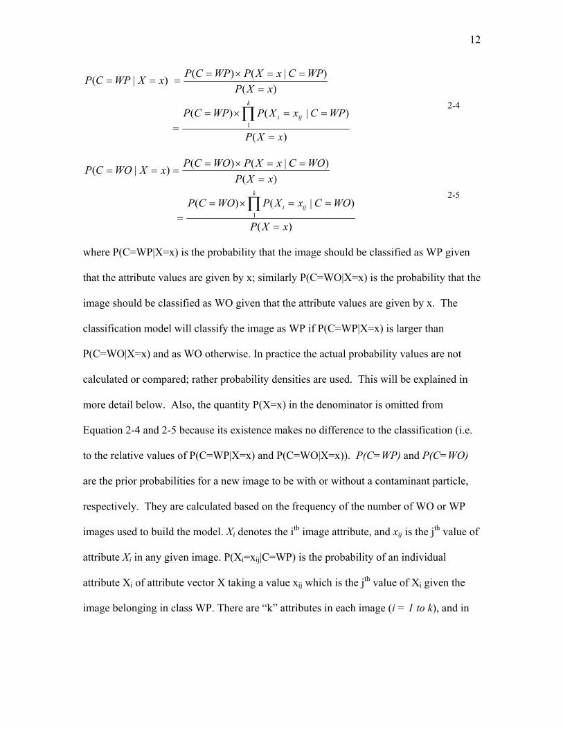
where P(C=WP|X=x) is the probability that the image should be classified as WP given
that the attribute values are given by x; similarly P(C=WO|X=x) is the probability that the
image should be classified as WO given that the attribute values are given by x. The
classification model will classify the image as WP if P(C=WP|X=x) is larger than
P(C=WO|X=x) and as WO otherwise. In practice the actual probability values are not
calculated or compared; rather probability densities are used. This will be explained in
more detail below. Also, the quantity P(X=x) in the denominator is omitted from
Equation 2-4 and 2-5 because its existence makes no difference to the classification (i.e.
to the relative values of P(C=WP|X=x) and P(C=WO|X=x)). P(C=WP) and P(C=WO)
are the prior probabilities for a new image to be with or without a contaminant particle,
respectively. They are calculated based on the frequency of the number of WO or WP
images used to build the model. Xi denotes the ith image attribute, and xij is the jth value of
attribute Xi in any given image. P(Xi=xij|C=WP) is the probability of an individual
attribute Xi of attribute vector X taking a value xij which is the jth value of Xi given the
image belonging in class WP. There are “k” attributes in each image (i = 1 to k), and in
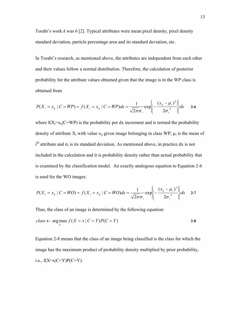
13
Torabi’s work k was 6 [2]. Typical attributes were mean pixel density, pixel density
standard deviation, particle percentage area and its standard deviation, etc.
In Torabi’s research, as mentioned above, the attributes are independent from each other
and their values follow a normal distribution. Therefore, the calculation of posterior
probability for the attribute values obtained given that the image is in the WP class is
obtained from
dxx
dxWPCxXfWPCxXPi
iij
iijiiji
⎪⎭
⎪⎬⎫
⎪⎩
⎪⎨⎧ −−====== 2
2
2
)(exp
21)|()|(
σ
μ
σπ 2-6
where f(Xi=xij|C=WP) is the probability per dx increment and is termed the probability
density of attribute Xi with value xij given image belonging in class WP; µi is the mean of
ith attribute and σi is its standard deviation. As mentioned above, in practice dx is not
included in the calculation and it is probability density rather than actual probability that
is examined by the classification model. An exactly analogous equation to Equation 2-6
is used for the WO images.
dxx
dxWOCxXfWOCxXPi
iij
iijiiji
⎪⎭
⎪⎬⎫
⎪⎩
⎪⎨⎧ −−====== 2
2
2
)(exp
21)|()|(
σ
μ
σπ 2-7
Thus, the class of an image is determined by the following equation:
)()|(maxarg YCPYCxXfclassY
===← 2-8
Equation 2-8 means that the class of an image being classified is the class for which the
image has the maximum product of probability density multiplied by prior probability,
i.e., f(X=x|C=Y)P(C=Y).

14
In Torabi’s research, the captured images from the Scanning Particle Monitor (SPM) can
be divided into two categories in terms of image quality: low background images (Figure
2-2 ) and high background noise images (Figure 2-3). Figure 2-2 shows an image with
microgel contaminants in polymer melt with no visible additive in the background. In
Figure 2-3, glass microsphere is present in polymer met with high background noise due
to the presence of talc additive.
To integrate the Intelligent Learning Machine (ILM) with Bayesian model, two
knowledge tables (KT) are created, one for calculating the probability of WP and the
other for calculating the WO probability. The WP knowledge table was formed with WP
images, and the WO knowledge table with WO images. During the incremental learning
period, when new image arrives, the human observer will determine whether an image is
WO or WP and then the measured attributes of the image will be added to the
corresponding knowledge table, and at the same time the model built based upon the
knowledge table will be updated accordingly.
Figure 2-2 Mircogel image with no additive in the background

15
Figure 2-3 Glass Microsphere (GMS) Images with talc additive in the background
In Torabi’s research, a Bayesian model was created off-line using 2000 training images
of microgel contaminant particles with low background noise such as in Figure 2-2. The
classification accuracy reached 95%. However, when this model was used to predict the
presence of glass-microsphere particles in the images with high background noise such as
image in Figure 2-3, the misclassification rate is as high as 50%. The reason for the poor
prediction performance is that the model was developed based on microgel images with
low background noise level but glass-microsphere images had a high background noise
level. Thus model built on microgel images detected the additives (i.e. the background
noise) of the glass-microsphere images as real particles. At the beginning of the test, the
error rate exceeded 50%. As the images of glass-microsphere particles with high
background noise were being captured, the human observer added 300 new images of
glass-microsphere particles with high background noise and known class label (WP or
WO) were added to the respective WP or WO knowledge table and the model was
updated through the ILM. The error rate in particle detection was measured after each
update. The software processing time for each image was less than 3 seconds. Therefore,

16
processing a set of 300 images required about 15 minutes. This process was repeated ten
times, and the classification error rate gradually dropped to 12% at the end of model
update. The change in classification error rate is shown in Figure 2-4 [2].
Torabi’s research developed a very practical real-time method for in-line image
classification by adapting the Bayesian model with a new invention of the Intelligent
Learning Machine (ILM). It is proved that the approach is able to rapidly adapt to a
variety of images captured in different imaging environment. The classification model is
updated in real-time, and there is no interruption of the process monitoring resulted.
Furthermore, the method proved to be extremely efficient and flexible without
compromising the quality or accuracy of the adapted model. However, the classification
accuracy by the adapted model is 92%, which is not very high. That means that this
0%
10%
20%
30%
40%
50%
60%
1 2 3 4 5 6 7 8 9 10 11 12 13 14 15 16 17 18 19 20 21 22 23Time
(Each interval is equivalent to 15 min or 300 Images)
Err
or r
ate
in im
age
clas
sific
atio
n (p
artic
le d
etec
tion)
Figure 2-4 Incremental Adaptation of Bayesian Classification Model
17
approach needs improvement: it is not sufficiently powerful in adapting to changing
image quality. This assessment can be further justified with the fact that a stand alone
static model built only with images of the high background noise level achieved a higher
classification accuracy of 92%. Thus, there is still a need to improve image quality
because the model alone can not provide a system of high classification accuracy to a
wide variety of images of different quality.
Image quality improvement entails image modification. Image modification is a complex
task because it involves a large number of operators. All available operators have their
own purpose of usage. To improve the quality of an image, it involves first the selection
of image operators from many candidate operators and then the determination of their
order of application. However, not only do the different operators have a different effect
on image quality so does their order of application matter. This already presents a
daunting task with high dimensionality. Therefore, part of the task of image quality
improvement is to reduce the dimensionality of image modification. Added to the
complexity is that each image operator has its own parameter setting, which needs to be
adjusted in order to achieve the desirable effect on image quality. More discussion on the
complexity of image modification will be followed in the Results and Discussions
chapter.
In this research, the goal is to improve image classification accuracy. Thus there is a need
to understand the relationship between image quality and classification, that is what is the
image quality required for improved classification.

18
Since the objectives of this thesis combine image processing and data mining, there is
very large amount of relevant literature. The emphasis in this section is on describing
the proposed strategy for accomplishing the objectives in the context of this literature.
2.3 Off-line Image Quality Modification
The first objective of this work is to develop an off-line automated method to determine
how to modify image quality of reference images. Reference images are those which are
typical images to be encountered but for which the software is informed as to whether the
image is in the WO or WP class. The sought modification is not to obtain an image that
appears most appealing to the human eye but rather to obtain an image that results in
better classification.
Thus, this section examines the literature with respect to how image quality has been
defined and modified.
2.3.1 Proposed Strategy for Accomplishing the First Objective
The proposed strategy for accomplishing this objective is:
i. Develop a general method for reducing the dimensionality of the task of
image quality improvement by selecting image quality operators (IQ
Operators) and their order of application. Image quality needs to be defined
using property measurements of an image: “Image Quality Metrics” (IQ Metrics).
A method of selecting the best ways of altering the IQ Metrics, Image Quality
Operators (IQ Operators), is then needed. This method should be applicable to a
wide variety of images and sufficiently broad in scope to initially include many
different IQ Operators.
19
ii. Given the IQ Operators and their sequence of application for a specific raw
image, develop a computer implemented method for determining the values
of parameters in these operators. Once image quality is defined and the IQ
Operators are selected, the parameters in these IQ Operators will be
systematically varied to obtain the optimal image quality.
iii. Formulate a “Reference Image Database”. Each optimized image will provide
two types of information: (a) a description of the raw image using IQ Metrics and
other necessary attributes related to objects of interest (such as particles) and (b)
instructions on how to transform the raw image into an optimized image by
specifying the image quality operators, their order of application and values of
their parameters. This information for all images provides the “Reference Image
Database” to be used to accomplish the second objective.
The following sections review the published literature relevant to this strategy.
2.3.2 Defining Image Quality: Image Quality Metrics Image quality metrics (IQ Metrics) are the quantitative values which define image
quality. Images are used for diverse purposes. Thus, in order to define the concept of
image quality in a reasonable manner, the underlying task of using the image should
generally be specified: an image can be defined to be of good quality if it fulfills its
intended task well. Image quality then becomes a task-dependent quantity. This is evident
in much of the literature [34-44]. For example, medical images are used as a means to
obtain information of the health status of the patient, and ultimately, clinical image
quality should be defined by the impact of the image on correct diagnosis or on the

20
outcome of the treatment of the patient. It could be thought that such a definition of
image quality would obscure matters: image quality is then not solely dependent on
image characteristics, but also on the specific task, the observer’s a-priori information on
the task and the observer’s ability to use both the prior information and the image
information for his decisions. These factors make image quality definition a challenging
problem. The choice of IQ Metrics is also dependent on the applications. In radiological
imaging, image noise is the most important quality-limiting factor in radiological
imaging, because it sets limits to the detectability of details and also restricts possibilities
with regards to obtaining the details visible by image enhancement (e.g., image
sharpening and contrast increase) [45]. However image noise is not very critical if the
object to be detected in an image is much larger than the noise in size.
Given the above situation, however, the formulation of IQ Metrics has continued to be
pursued because the explosive growth of digital imaging has led quality metrics to be
applied in various fields. Image properties such as noise, sharpness and contrast lead to
many objective image quality definitions [37, 38, 40-42, 46-48]. The understanding of the
human visual system leads to many subjective image quality definitions [35, 37, 40-44,
47, 49]. In the subjective definitions, human perception become paramount, and IQ
Metrics are correlated with the preference of an observer. The dilemma is that many
objective IQ Metrics do not correlate well with subjective IQ Metrics. As a result, a great
deal of effort has been made in recent years to develop objective IQ Metrics that correlate
well with subjective quality metrics [38, 40, 42, 44, 50] by incorporating the human
visual system into the objective IQ Metrics. Unfortunately, only limited success has been

21
achieved. In this review, the emphasis will be on objective IQ Metrics since they are
more suitable than subjective IQ Metrics for real-time process monitoring.
Generally speaking, IQ Metrics have two main uses: quality control [3, 6, 10, 13, 16, 51]
and benchmarking image processing methods [40-42, 44].
Objective IQ Metrics, in general, can be divided into two groups: reference and no-
reference IQ Metrics. Reference objective IQ Metrics need a reference image (often the
original image) to calculate the metrics. Because of this, they are also called bivariate
metrics. Most of the reference objective IQ Metrics exploit the deviations between the
corresponding pixels in the reference image and the processed or degraded images. No-
reference objective IQ Metrics do not require a reference. Thus they are also called blind
IQ Metrics. Reference objective IQ Metrics have gained much attention [34, 35, 40, 41,
44] in image processing because they are suitable for evaluating the performance of
image processing algorithms, particularly compression and filtering methods. Appendix I
provides an overview of Objective IQ Metrics that do and do not require a reference.
It is evident that IQ Metrics that do not require a reference are preferred for in-line
monitoring applications. Reference images may not always available for real-world,
and, in particular, real-time applications. Also, in-line monitoring requires high-speed
processing that synchronizes well with the changes in the monitored process. This means
that the selected IQ Metrics should be simple computationally as well as efficient and
reliable.
For this purpose, no-reference IQ Metrics are more suitable than reference IQ Metrics.

22
Changing the values of IQ Metrics requires Image Quality Operators (IQ Operators).
These are the subject of the next section.
2.3.3 Image Quality Operators (IQ Operators) There are a large number of well established image quality operators (IQ Operators)
available. Image quality operators are usually divided into two major categories:
radiometric and geometric [52]. Radiometric operators, also called pointwise operators,
act on the original image by changing its brightness distribution. With geometric
operators, the grey value in each pixel of the image is changed according to its
neighborhood. Details on the most important image quality operators are summarized in
Appendix II.
ImageJ, the software used in this work, for example, has 54 different operators. When it
is realized that most operators contain their own adjustable parameters, that they can be
applied more than once, and that their order of application affects the results on the
image, it can be seen that the dimension of the operator selection problem is staggering.
A strategy for their application is needed.
Selection of the appropriate IQ Operators, the correct values of their individual
parameters and their order of application represents a sizable data screening problem.
Identification of irrelevant IQ Operators and elucidation of inter-dependence amongst the
various IQ Operators are particularly important.
Over the years, many systems and methods have been developed for image analysis [53-
63]. Many of these systems have been reported to work well on specific types of image

23
analysis tasks. The way in which image expertise and knowledge are incorporated into a
system varies widely from one system to another, with little systematic generalization
reported. It has been a common practice for researcher and system designers to design
new systems or to modify existing systems to solve their own image analysis problems
through a process of trial-and-error experimentation. Despite many efforts to develop a
general vision system [64] such systems developed have failed to compete with domain
or problem-specific systems in solving practical image analysis problems.
A compromise between a problem specific system and a general vision system is a
flexible specific system, which is not universal but that can adapt to quite a wide range of
practical problems. In the past two decades, there have been many attempts to construct
such systems [65-72]. Most of these systems are knowledge-based with the support of
artificial intelligence (AI) planning technique. There are two types of knowledge: the
knowledge independent of the content of a given image; and the knowledge dependent on
it. The former is the knowledge of image data types and image processing algorithms
(operators). The latter is based on the image processing expertise of experts. These two
types of knowledge alone are not enough to generate an image processing process.
From these literature there is no real guidance how best to automatically use IQ Operators
to improve performance of an image classification model. The primary difficulty in this
work is defining image quality so that it is relevant to classifier performance. An image
that appears superior to the human eye may not be considered superior to the
classification model! The struggle to define image quality is a significant part of what
was done to accomplish the first objective of this thesis and will be detailed in the Results
and Discussion.

24
In this research the aim was to define image quality with a single number and to use a
numerical optimization program to adjust the parameters in the Image Quality Operators
in order to maximize image quality for each individual image. In this case the Nelder
Mead Simplex Optimization method was used.
2.3.4 Optimizing Image Quality Once the IQ Operators and their order of application have been selected for a specific raw
image the problem is to rapidly determine the best values of the parameters in the IQ
Operators so as to obtain the highest quality image. An optimization method will need to
systematically change the parameter values and evaluate the image quality following
each change. A wide variety of optimization methods are available. However, the
Nelder Mead Simplex method appears particularly attractive. The method tolerates
experimental error very well in obtaining the optimum. This is an important aspect in this
work because of between image scatter. It has been used for both numerical optimization
and sequential experimental design but not for image analysis. It is essentially a “logical
guessing” program. Here it systematically guessed the values of the parameters,
modified the image, computed image quality and iterated until image quality was a
maximum. It accelerates towards the optimum and it does not require calculation of
derivatives. The algorithm depends only on the relative value of results obtained in each
trial. Disadvantages of the method are that it may fail or at least become very inefficient
if large numbers of IQ Operators are selected. The Simplex method is reviewed and
described in greater detail in Appendix III.

25
2.4 In-line Image Quality Modification As mentioned above, the second objective is “to develop an in-line method for modifying
the quality of acquired images to permit improved classification by using the results of
the first objective as a database”.
2.4.1 Proposed Strategy for Accomplishing the Second Objective The proposed strategy for accomplishing this objective is as follows:
i. Locate the reference image in the Reference Image Database most closely
resembling newly acquired image.
The IQ metrics of newly acquired image need to be compared with each image in
the Reference Image Database to obtain the most similar reference image in each
case. Combining and comparing these IQ Metrics involves defining raw image
quality so that the most similar reference image can be located.
ii. Improve the quality of newly acquired image and assess the classification
performance.
In this case newly acquired image is modified and classified using the Torabi
Bayesian model trained on optimized images.
iii. Devise how to adapt image quality modification to deal with variable raw
images, combine this with Torabi’s adaptive Bayesian classification and assess
the performance.
This requires developing and implementing an adaptive image quality modification
combined with adaptive Bayesian classification model and assessing the effect on

26
classification. The assessment will employ a wide variety of images from the scanning
particle monitor.
2.4.2 Use of the Reference Image Database: Case-based Reasoning Case Based Reasoning (CBR) is ideally suited to utilizing the Reference Image Database
in order to locate the reference image most similar to a newly acquired image along with
the accompanying instructions on how to use the IQ Operators to optimize the new
image.
Case-based Reasoning (CBR) is an approach in which new problems can be solved by
reusing solutions to past solved problems. Past cases or problems represent valuable
knowledge, especially in a weak theory domain in which the relationship of cause and
effects may not be well understood. In the fields of artificial intelligence and machine
learning, CBR has been described as a model for conducting Artificial Intelligence (AI)
research, and as a knowledge engineering methodology for deploying practical intelligent
systems [73]. In fact, CBR has been applied to a full spectrum of Artificial Intelligence
tasks, including classification, scheduling, planning, design and diagnosis.
In the past decade or so, CBR has gained popularity in many domains because of the
generality of the idea. The key areas that have seen its application are medicine [74], law
[75], education [76], knowledge management [77], image processing and interpretation
[78-85]. While some artificial intelligence and machine learning techniques have stayed
in the laboratory for decades, producing research prototypes before commercialization,
CBR has provided solutions to many engineering applications from its infancy. CBR

27
systems for engineering application save millions of dollars in production costs and
demonstrate their effectiveness and applicability in diverse domains.
The first successful milestone application of CBR was Lockheed’s CLAVIER system
[86, 87]. The system is used to advise engineers of the loads of composite material parts
in large autoclave curing ovens. It has been in daily use since 1994 and it is a very
important system because it possesses all four elements of a typical CBR system:
retrieval, reuse, revision and retention. It is interesting because it was put into use only
after the failure of mathematical modeling and expert systems to solve the problem.
Another fielded engineering application of CBR is an innovative project called Cassiopee
[88]. The project developed a software system to support fault diagnosis of the CFM 56 -
3 aircraft engine used in the Boeing 737. The system uses case-based reasoning which
exploit failure descriptions that are stored in a case base. The system is used by airline
maintenance staff and CFMI specialists as a troubleshooting support.
Among other notable engineering CBR systems are the plastic colour matching system
for selecting a recipe of pigments that match a customer’s requested colour and has been
in use since 1996 at multiple General Electrical plastic sites [89], an on-line distributed
case-based reasoning system for estimating the cost of residential air conditioning system
in Western Australia [90] and a system called ICARUS (Intelligent Case-based Analysis
for Railroad Uptime Support) [91] which diagnoses locomotive faults and determines
probable causes for the faults and repair actions to correct the cause of the faults using
historical cases as reference. ICARUS was fielded in 1997 and has been in constant use
since that time. Recently, CBR has seen emerging applications in molecular biology,
28
such as the problem of analyzing genomic sequences and determining the structure of
proteins [92]. Another significant emerging area in bioinformatics and medical
informatics for CBR is the area of image analysis [80, 93].
The advantages of CBR over other machine learning techniques lie in a few aspects:
knowledge acquisition, knowledge maintenance, increasing problem-solving efficiency,
increasing quality of solution and extensibility. These are examined in the next section.
2.4.2.1 Advantages of Case-Based Reasoning The classic method for knowledge acquisition for a traditional knowledge-based system
(KBS) is through rule elicitation and formalization. The rule acquisition process can be
laborious and unreliable, especially when a large set of rules is required to meet the need
of a system. CBR does not generalize rules from cases. Therefore, the cost of knowledge
acquisition for CBR is very low [87]. However, CBR does require considerable initial
effort in gathering information and building up a case base. After the initial knowledge
base is created, it is often not difficult to augment and maintain the knowledge a CBR
system needs.
As with Artificial Intelligence (AI) applications, knowledge acquisition is just the initial
step towards a successful knowledge-based system (KBS). Without exception,
knowledge maintenance is required to refine and revise the previous knowledge and add
missing knowledge to a case base. In this sense, knowledge maintenance is an extension
of knowledge acquisition. CBR provides an important benefit for knowledge
maintenance because a user can add a new case to the case database without ruining the
29
functionality as is the case in a rule-based system. Because CBR, by nature, is an
incremental learning system, it can be readily expanded if the current case base is
insufficient to handle a new type of problem.
The reuse of past experience/solutions in CBR improves problem-solving efficiency
because a new solution will be building on prior solutions rather than repeating the effort
from the beginning. More than upgrading problem-solving efficiency, CBR also increases
the quality of solutions when a system is not well understood. The solution suggested by
CBR could be more accurate than those imperfect rules because cases reflect what
happened in reality.
Another vital benefit that CBR offered is its extensibility (or scale-up capability) to larger
problems. Its extensibility has now being tested in applications. The Cassiopee system
mentioned above, a case-based diagnostic aid for jet engines, uses 16,000 cases for its
diagnosis process [88]; and ALFA, a case-based system for power plant load forecasting,
is in operation with a case library of 87,000 cases [94].
In this work, CBR is to be used to select image processing requirements for new images.
The use of CBR in image interpretation is examined in the next section.
2.4.2.2 Case-Based Reasoning in Image Interpretation In general, image interpretation often requires many levels of sequential processing.
These many-levels of processing add complexity to the image interpretation system
because the result of processing at one level strongly depends on the performance of the
preceding level. Thus, image interpretation system is often domain specific and works

30
only under certain conditions and image quality. However, for a real-world image
monitoring system, environmental conditions change and noise can suddenly appear in
the images. Such difficulties present challenges and demand adaptability in image
interpretation.
Case-based reasoning potentially can meet such challenges because it is able to update
the case base and learn new knowledge incrementally. Examples include computer
tomography (CT) [80, 82, 85], in microscopy in diagnostic histopathology [95], in
myocardial scintigrams for automated detection of coronary heart disease [96], in
ultrasonic B-scans [97], in the development of image processing steps for image
processing problems not yet solved [78] and ultrasonic images [84]. However, the
application of CBR in image interpretation is still in its early stage. The types of images
to which CBR has been applied are mainly limited to medical images. There is no
reported application of CBR to images of particles. The application of CBR in image
interpretation has not been used for in-line image monitoring and real-time applications.
Although, as can be seen from the proceeding sections, CBR is potentially a very
powerful method, there are some issues. These include: case representation of image,
selection of similarity attributes, similarity measures, case maintenance (addition and
deletion) and incremental learning. The following sections examine these issues with
emphasis on CBR application in this work.
2.4.2.3 The Case-Based Reasoning Process CBR methodology is based upon two assumptions. The first assumption is that similar
problems have similar solutions. Accordingly, solutions for similar past problems are

31
useful for new problem-solving. The second assumption is that, in a specific context or an
application system, the same types of problems tend to recur. Therefore, future problems
are similar to prior problems [98]. If these two assumptions are true, remembering the
prior problems and their solutions and reusing or revising them for solving new problem
can then be a very effective problem solving method.
In the Case-based Reasoning (CBR) community, CBR tasks are divided into two classes:
interpretive CBR and problem-solving CBR [73, 98]. Interpretive CBR uses prior cases
as reference points for classifying or for characterizing new situations; problem-solving
CBR use prior cases to infer solutions that could apply to new cases. In this literature
review, the focus is problem-solving CBR since it is more relevant to one of the
objectives of this research – to develop an automated method for modifying the image to
the image quality required for improved classification results.
A classic CBR model suggested by [99] is shown in Figure 2-5. The search for a solution
to a new problem (i.e., a new case) involves obtaining a problem description, measuring
the similarity of the new problem to prior problems stored in a case database (often
termed a “knowledge base”), retrieving one or more similar cases and attempting to reuse
the solution of one of the retrieved cases (or if necessary adapting it to the situation
presented by the new problem). The solution proposed by the system is then evaluated. If
the evaluation requires, the proposed solution is then revised and becomes a confirmed
solution. Depending on the updating scheme adopted, the new problem and its solution
can then be retained as a learned case and added to the case database for future use.
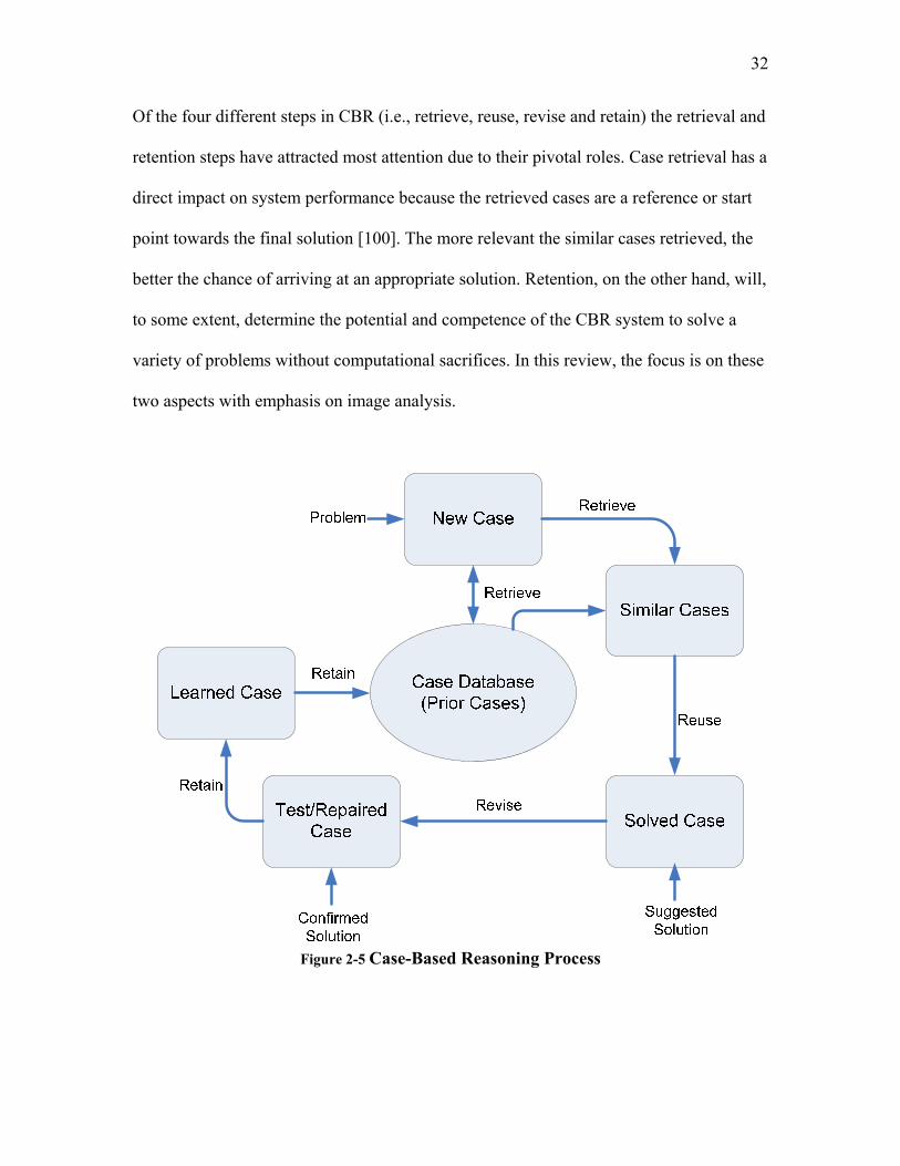
32
Of the four different steps in CBR (i.e., retrieve, reuse, revise and retain) the retrieval and
retention steps have attracted most attention due to their pivotal roles. Case retrieval has a
direct impact on system performance because the retrieved cases are a reference or start
point towards the final solution [100]. The more relevant the similar cases retrieved, the
better the chance of arriving at an appropriate solution. Retention, on the other hand, will,
to some extent, determine the potential and competence of the CBR system to solve a
variety of problems without computational sacrifices. In this review, the focus is on these
two aspects with emphasis on image analysis.
Figure 2-5 Case-Based Reasoning Process

33
2.4.2.4 Case Retrieval in Image Interpretation As pointed out above, case retrieval is an important step in the CBR process. It involves
identifying attributes, searching the case database, calculating similarity and selecting the
similar cases using defined criteria [99]. Many CBR systems deploy a two-step retrieval
approach, first retrieving a set of promising candidate cases, and then implementing a
“finer-grained” evaluation of the similarity of the retrieved cases and the new case.
Identification of Similarity Attributes The attributes to be used in CBR are domain specific. The determination of the correct
attributes to compare is sometimes not very clear. Decisions about which attributes are
important are often based on explanations of attribute relevance.
In image analysis and processing, attributes could consist of non-image information and
image information [101]. In general, attributes can be numerical, categorical or symbolic.
The attributes used to describe an image case depend on the type of image and the task of
image interpretation. For an example, for CT images, non-image attributes of patient
information such as age, sex, slice thickness and number of slices were used by Perner
[80]. In a railway inspection application [83], the type of sensor for capturing ultrasonic
image was considered an important non-image attribute. Other image acquisition
attributes such as illumination of the scene, and information about the objects could be
considered non-image information as well. Image related attributes adopted include the
pixel matrix itself [102], objects contained in the image and their attributes, as well as the
spatial relation between the objects. A four-level hierarchy representation of an image
34
case was developed [97]. At the lowest level, attributes are objects described by their own
attributes such as location, orientation, type (line, parabola or noise) parameters. At the
highest level the attribute is the image scene. This hierarchy attribute-based
representation of image allows matching the case in the case base on different granularity
levels. Other high-level abstraction attributes extracted from an image are also used to
represent a case. The noticeable attributes are numerical properties of the image, such as
the statistical measures of the grey level, including mean, variance, skewness, kurtosis,
variation coefficient, energy, entropy, first-order histogram, and centroid.
Using of Similarity Attributes for Similarity Measurement
With the identification of attributes, CBR then relies on similarity assessment to calculate
the distance between previous cases and the current case. However, the attributes and
similarity measure are tightly coupled. For example, some attributes are symbolic and can
be used qualitatively but not quantitatively. Two major similarity assessments are
proposed in image interpretation: surface similarity and structural similarity. The
selection of attributes amongst these two assessments depends on the case representation
of a specific application. In some applications, surface similarity is adequate for
measuring the similarity of the stored case to the target problem. In other applications,
cases are represented by complex structures such as graphs and consequently require
assessment of the structural similarity to retrieve cases.
Surface similarity uses attributes. These attributes are often attribute-value pairs. In
surface similarity, the similarity of a case in a case base to the current case is computed
using the selected attributes and the similarity measure is given as a real number.
35
In image analysis, depending on the image representation, similarity measure can be
divided into three categories. First, pixel-matrix based similarity measures; second,
attribute-based surface similarity measures (either numerical [80], symbolic or mixed
type); and last, structural similarity measures [96, 102-104].
Perner (1999) calculated the similarity measure by combining the non-image similarity
and image similarity for automatic CT image segmentation. She defined a similarity
measure for image information in the following equation:
∑= −
−−
−−
=k
i ii
iiB
ii
iiAi CC
CCCC
CCw
kdistAB
1 minmax
min
minmax
min1 2-9
where CiA and CiB are the ith attribute values of image A and B, respectively. Cimin and
Cimax are the minimum and maximum values of the ith attribute, respectively. wi is the
weight assigned to the ith attribute with the sum of wis equal to unity. k is the number of
attributes. The attributes used are statistical measures of the grey level including mean,
variance, skewness, kurtosis, variation coefficient, energy, entropy, and centroid.
Euclidean distance, as shown in Equation 2-10, is used to calculate similarity in other
application domains such as manufacturing process of printed circuit board [105] but not
in image interpretation.
∑=
−=k
iiBiA CCdistAB
1
2)( 2-10
where CiA and CiB are the ith attribute values of image A and B, respectively. K is the
number of attributes.
A structural similarity measure introduced by [102] was applied in image segmentation
[80]. The similarity measure takes the image matrix itself and calculates the similarity
36
between the two image matrices. The calculation of similarity is an average of distances
for all pixels in one image to the corresponding pixels at the same location in the other
images. The measure reflects the structural similarity of two images. It requires the
storage of images in the case base.
2.4.2.5 Case Retention in Case Based Reasoning Retention involves the update of case base with newly learned cases, thus it is the
learning part of the CBR process. Retention enables the system to learn new cases, which
in turn enhance the competence of the system in dealing with new problems. There are
two aspects of retention, success-driven learning and failure-driven learning [98].
For success-driven learning, the resulting solution for a successful CBR process is stored
in the case base for future reuse. In this way, success-driven learning favors cases that
more likely to lead to success. The stored successful cases thus will increase the capacity
of the system to solve problems which the system might not be able to solve previously.
However, success-driven learning can cause redundancy in the case base. That is, some
very similar cases with very similar solution could be retained into the case base. This in
turn could increase the search time in case retrieval.
For failure-driven learning, CBR values the failed cases as well as the successful cases.
The rational behind this is that failures indicate that learning is needed. In addition,
failures reveal what is needed to be learned to avoid future failure. In failure-driven
learning, the initial knowledge acquisition and the filling of the case base is success-
driven with successful cases added to the case base. After the case base is big enough, the
CBR system starts to learn from failure, in which the solution obtained through the CBR

37
process does not work. This failure is called task failure by Leake [98]. The failed case is
then subject to repair outside the CBR process until a successful solution is found. This
case, with its new solution, is then retained and added to the case base. In essence, this is
still learning from successes but it employs a repaired solution.
Different from task failure, expectation failure addresses the scenario that the system
expects that a solution to a new problem will work but it does not. The expectation
failure could help to avoid a similar problem in the future by suggesting that the system
learns to predict it in advance.
For an image interpretation system, case base maintenance has not yet been extensively
studied. Jarmulak [97] adds new case to the case base, splits the case base into clusters of
fixed size and use a prototype to represent them in the hope of speeding up the search
process. Perner also updated the case base with newly learned cases and adopted a way of
learning of case classes and prototypes[80, 106]. It has been suggested that the deletion or
forgetting of cases is not preferable in image interpretation. In addition, Perner
recommends that distorted and very noisy images and images with illumination defects
should not be added to the case base if the image analysis or reasoning process cannot
handle it.
2.4.2.6 Computation Efficiency of Case-Based Reasoning The Computation efficiency in CBR is closely related to the organization of case base
which has a direct effect on retrieval time. If a case base is flat and very large, it will take
time to calculate the similarity measure between the current problem case and each case

38
in the case base. Consequently, a flat case base is to be avoided in order to speed up the
case retrieval process. An alternative to flat case base is to create a hierarchical case base
such as a decision-tree-like structure proposed by McSherry [107] and hierarchical
clustering by Perner [106]. In this fashion, similar cases are grouped together under the
same branch. This organization allows separation of a group of similar cases from that of
non-similar cases at the earliest stage of the retrieval process.
In case of a flat case base, parallel computing is considered a viable approach but
obviously the requirement of expensive hardware is a drawback.
For CBR applications in image analysis, it is generally considered that the computation
workload is not a critical issue if the case is represented by high-level numerical
attributes instead of the image matrix itself [93].

39
2.5 Evaluation of Classification Methods This work aims at improving classification of images by modifying image quality. As
will be seen in subsequent sections, comparison of different classification results is
necessary when comparing different definitions of image quality and the same
classification model or when comparing different classification models. There are many
measures that can be used to accomplish such a comparison. The most basic summary of
classifier performance is a “confusion matrix”. As shown in Table 2-1 for the binary
class situation (WO or WP) of this work, each element of the matrix shows the number of
images for which the actual class is given by the label for the row and the predicted class
is given by the label for the column. The elements of this matrix are used to provide a
variety of calculated measures of classification. These are summarized in Table 2-2 and
Table 2-3. Table 2-2 shows the confusion matrix using the data mining terminology for
the basic measures of the table. Table 2-3 shows definitions and the many measures
obtainable from the confusion matrix.
When classification results are to be examined in this work the first result presented is the
confusion matrix. Attention is then drawn to the following measures defined in detail in
Table 2-3 :
1. Classification Error Rate: the fraction of cases (either actual WO or actual WP)
not correctly classified is an extremely important measure. It provides an overall
view of the classification. It will be seen that most of the classifications can be
done with better than 90% accuracy. It is the last 10% of classification accuracy,
i.e. the classification error rate, that is extremely important in many process

40
control situations. Under some circumstances it can mean the difference between
erroneously shutting down an extrusion line 10% of the monitoring time versus
less than 1% of the monitoring time. Therefore, reduction of classification error
is of utmost importance.
2. False Positive Rate: erroneously identifying images that have no particle as
having a particle means causing a false alarm in a process control situation. The
false positive rate expresses the number of incorrectly classified WO as a fraction
of the number of WO images.
3. False Negative Rate: erroneously identifying images that have a particle as
having no particle means allowing off-specification product to be produced. This
error would generally be expected to have worse consequences than the false
alarm of a false positive rate.
In this work classification error, false positive rate and false negative rate are presented in
a bar graph and are compared against another classification in the same graph.
Table 2-1 Confusion Matrix for a Binary Classification Problem
Predicted Class is WP Predicted Class is WO
Actual Class is WP # of Images that are Actually WP and are
Predicted as WP
# of Images that are Actually WP but are
Predicted as WO Actual Class is WO # of Images that are
Actually WO but are Predicted as WP
# of Images that are Actually WO and are Predicted as
WO Table 2-2 Confusion Matrix for a Binary Classification Problem Showing Data Mining Measures
Predicted Positives Predicted Negatives Actual Positives (P) True Positives (TP) False Negatives (FN)
Actual Negatives (N) False Positives (FP) True Negatives (TN)
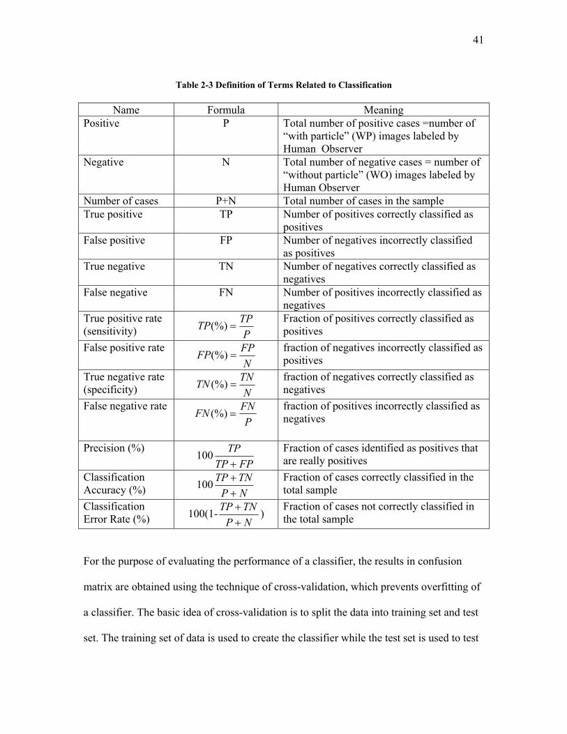
41
Table 2-3 Definition of Terms Related to Classification
Name Formula Meaning
Positive P Total number of positive cases =number of “with particle” (WP) images labeled by Human Observer
Negative N Total number of negative cases = number of “without particle” (WO) images labeled by Human Observer
Number of cases P+N Total number of cases in the sample True positive TP Number of positives correctly classified as
positives False positive FP Number of negatives incorrectly classified
as positives True negative TN Number of negatives correctly classified as
negatives False negative FN Number of positives incorrectly classified as
negatives True positive rate (sensitivity) P
TPTP =(%) Fraction of positives correctly classified as positives
False positive rate NFPFP =(%)
fraction of negatives incorrectly classified as positives
True negative rate (specificity) N
TNTN =(%) fraction of negatives correctly classified as negatives
False negative rate P
FNFN =(%)
fraction of positives incorrectly classified as negatives
Precision (%) 100
FPTPTP+
Fraction of cases identified as positives that are really positives
Classification Accuracy (%) 100
NPTNTP
++
Fraction of cases correctly classified in the total sample
Classification Error Rate (%) 100(1-
NPTNTP
++ )
Fraction of cases not correctly classified in the total sample
For the purpose of evaluating the performance of a classifier, the results in confusion
matrix are obtained using the technique of cross-validation, which prevents overfitting of
a classifier. The basic idea of cross-validation is to split the data into training set and test
set. The training set of data is used to create the classifier while the test set is used to test

42
the predictability of the classifier in terms of accuracy or error rate. There are three main
types of cross-validation: test set (also called “hold-out estimation set”), leave-one-out
and k-fold cross validation. These three methods differ in how the data set is divided
between training set and test set and how error is evaluated. The test set method randomly
chooses a certain percent of the data and retains the remainder of the data as a training
set. The classification results are attained by applying the classifier to the test set data.
The classification errors for the test set are reported in the confusion matrix. The leave-
one-out cross validation (LOOCV) method leaves one data record out at a time for testing
and the rest of the data records are used for training. All data records in the data set are
used exactly once for testing. When all data records have been used for testing, the errors
are summed and reported in the confusion matrix for the classifier. The test-set method is
simple and computationally inexpensive but it is vulnerable to the variance of the
selection test set, which results in unreliable future predictability. In contrast, LOOCV
uses all data points both for training and testing but it is very computationally expensive.
The K-fold cross validation technique takes advantage of the benefits of both the test set
method and LOOCV by randomly breaking the data into k partitions. Each partition is
successively selected for testing once while the remainder of the partitions are used for
training. The classification errors for each partition when it is used as a testing set are
summed and reported in the confusion matrix. The number of partitions (the “k value”)
will have an effect on the accuracy (proximity to the true value) and variance (variability)
of the estimated error rates. With a large k value, the accuracy tends to be high but the
variance is large. For a small k value, the accuracy tends to be low while the variance is
small [108-110]. In practice, the choice of the number of folds depends on the dataset
43
size. For a medium size dataset, the most popular k-fold cross validation is 10-fold [108-
110]. This value will be used throughout this work for evaluating classifiers since we
have medium-size training sets of less than 800 training data records.
Finally, for examining classifier performance, in addition to the confusion matrix,
classification error, false positive rate and false negative rate, this work shows a “receiver
operating characteristic” curve (commonly referred to as a ROC curve).
Figure 2-6 illustrates the receiver operating characteristics (ROC) curve using results
from one of the classifiers used in this work. The ROC curve is a plot of true positive rate
(on the y axis) versus the false positive rate (on the x axis). This type of curve was
originally used in signal theory to select an operating point to distinguish the absence or
presence of signal. In a ROC figure, the upper left point (0,1) represents the best possible
classification since it represents a 100% true positive rate and a zero false positive rate.
The point (1,0) at the bottom right corner of the ROC figure represents the worst
classification with a zero true positive rate and a100% false positive rate. The diagonal
line represents a random classifier since it shows a 50% true positive rate and a 50% false
positive rate for the whole range of values on the axes. The important characteristic to
note is that the left top region of the figure is where the best classifier performance lies.
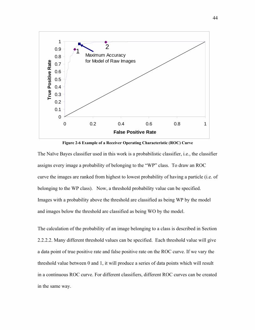
44
00.10.20.30.40.5
0.60.70.80.9
1
0 0.2 0.4 0.6 0.8 1
False Positive Rate
True
Pos
itive
Rat
eMaximum Accuracyfor Model of Raw Images
12
Figure 2-6 Example of a Receiver Operating Characteristic (ROC) Curve
The Naïve Bayes classifier used in this work is a probabilistic classifier, i.e., the classifier
assigns every image a probability of belonging to the “WP” class. To draw an ROC
curve the images are ranked from highest to lowest probability of having a particle (i.e. of
belonging to the WP class). Now, a threshold probability value can be specified.
Images with a probability above the threshold are classified as being WP by the model
and images below the threshold are classified as being WO by the model.
The calculation of the probability of an image belonging to a class is described in Section
2.2.2.2. Many different threshold values can be specified. Each threshold value will give
a data point of true positive rate and false positive rate on the ROC curve. If we vary the
threshold value between 0 and 1, it will produce a series of data points which will result
in a continuous ROC curve. For different classifiers, different ROC curves can be created
in the same way.

45
While only classifier accuracy (or error rate) is used to measure the performance of a
classifier, it does not take into consideration the fact that the number of false positives
and false negatives may differ. Also, the cost of errors for false positives (false alarm)
and false negatives are not the same in many applications. In addition, two data points
can have the same accuracy in a ROC curve such as data points marked “1” and “2” in
Figure 2-6. For these reasons, the area under the ROC curve (AUC) has been recently
considered by many to be a statistical consistent measure of the goodness of separation of
classes by a classifier because it reflects the probability or ranking information of training
cases while a single number of accuracy (shown as one data point in a ROC curve) does
not possess. Overall, the bigger the AUC, the more discriminating is a classifier.
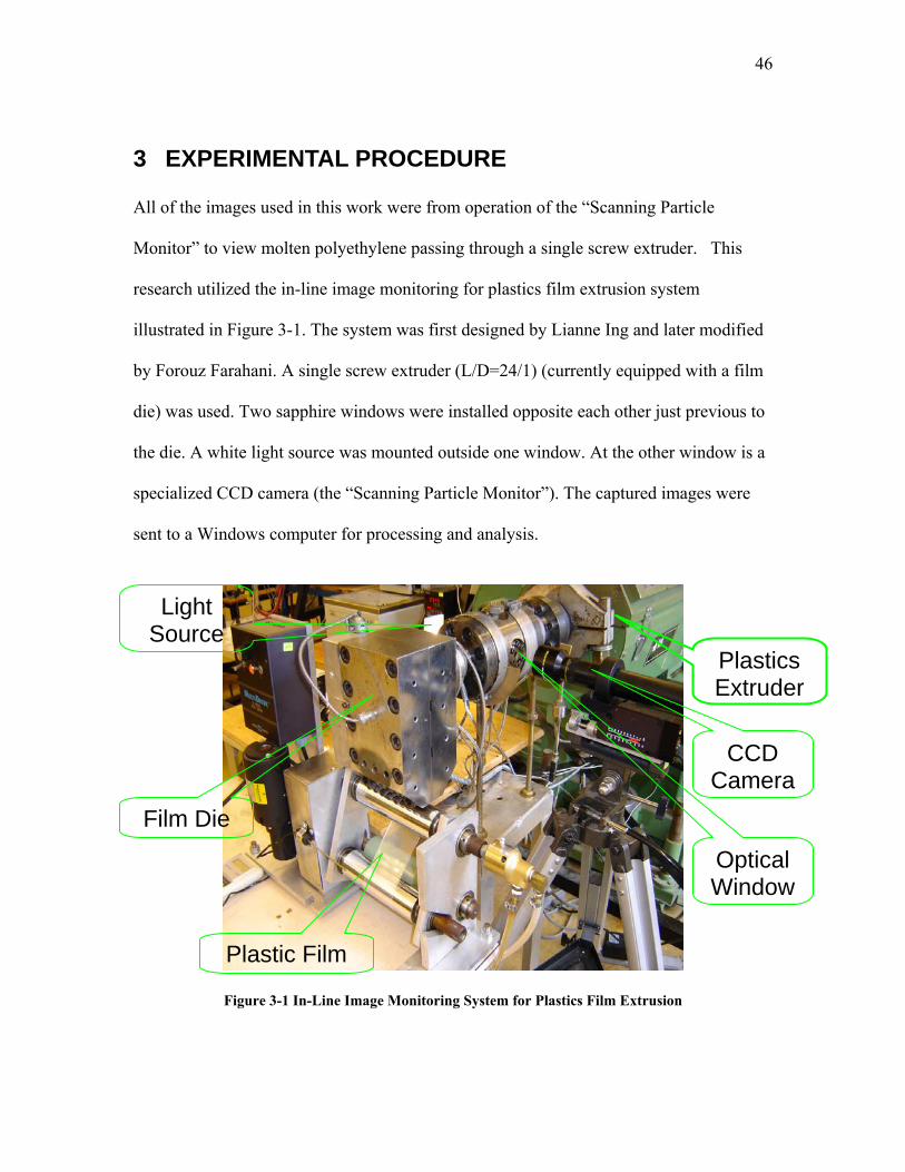
46
3 EXPERIMENTAL PROCEDURE All of the images used in this work were from operation of the “Scanning Particle
Monitor” to view molten polyethylene passing through a single screw extruder. This
research utilized the in-line image monitoring for plastics film extrusion system
illustrated in Figure 3-1. The system was first designed by Lianne Ing and later modified
by Forouz Farahani. A single screw extruder (L/D=24/1) (currently equipped with a film
die) was used. Two sapphire windows were installed opposite each other just previous to
the die. A white light source was mounted outside one window. At the other window is a
specialized CCD camera (the “Scanning Particle Monitor”). The captured images were
sent to a Windows computer for processing and analysis.
Figure 3-1 In-Line Image Monitoring System for Plastics Film Extrusion
Plastics Extruder
Film Die
Plastic Film
CCD Camera
Optical Window
Light Source

47
Table 3-1 summarizes the digital images used in this work. Image Set 1 is that used by
Torabi in his research. Image Set 2 is produced by Ing in her research, and Image Set 3
was generated in this work from extrusion runs. Material feed (the polymer pellets feed)
to the extruder and operating conditions (such as lighting, extruder running speed and
heating temperatures) were different for each image set.
Table 3-1 Summary of Image Data Sets Used in This Work
Image Data Set
Number of Images
Description Origin
Image Set 1 4294 Images generated with grade 530A polyethylene pellets feed made by Dow Chemical but with the injection of different kinds and concentration of particles to the feed.
Keivan Torabi
Image Set 2 1344 Images generated with polyethylene pellets feed of high concentration microgel made by Exxon
Lianne Ing
Image Set 3 2010 Images generated with grade 530A polyethylene pellets feed made by Dow Chemical with injection of different kinds, sizes and concentration of particles to the feed; Also image generated with polyethylene pellets feed of high concentration additive made by Exxon.
This work
The final set of images, Image Set 3, were images produced by extrusion experiments run
especially for this work with the objective of obtaining images of diverse image quality.
A summary of extruder running conditions used for these experiments is shown in Table
3-2. The experimental runs utilized two different grades of polyethylene pelletized feed.
The first (Runs 3-1 to 3-4) was grade 530A polyethylene produced by Dow Chemical.
For this grade, two different sizes of glass microspheres (GMS) (30 micron in run 3-2 and
100 micron in run 3-3) and variable sized glass bubbles (as in run 3-4) were added as a

48
“pulse input” to the feeds. The weight concentration of 30µm GMS is 200ppm while that
of 100 µm GMS is 40ppm. The second kind of pellets feed was high additive content
polyethylene pellets feed from Exxon (runs 3-5 and 3-6). Glass beads were injected into
the feed in run 3-6.
Table 3-2 Image Data Sets Produced from Experimental Extrusion Runs in this Research
Run Number Number of
Images Extruder Feed Pellets Particles Injected
3-1 269 530A Polyethylene from Dow Chemical
No particles injection
3-2 403 530A Polyethylene from Dow Chemical
30 µm – 200 ppm glass microsphere
3-3 400 530A Polyethylene from Dow Chemical
100 µm – 40 ppm glass microsphere
3-4 400 530A Polyethylene from Dow Chemical
20 ppm Variable size glass bubbles
3-5 195 High additive polyethylene from Exxon
No particles injection
3-6 343 High additive polyethylene from Exxon
75 µm – 20 ppm glass beads
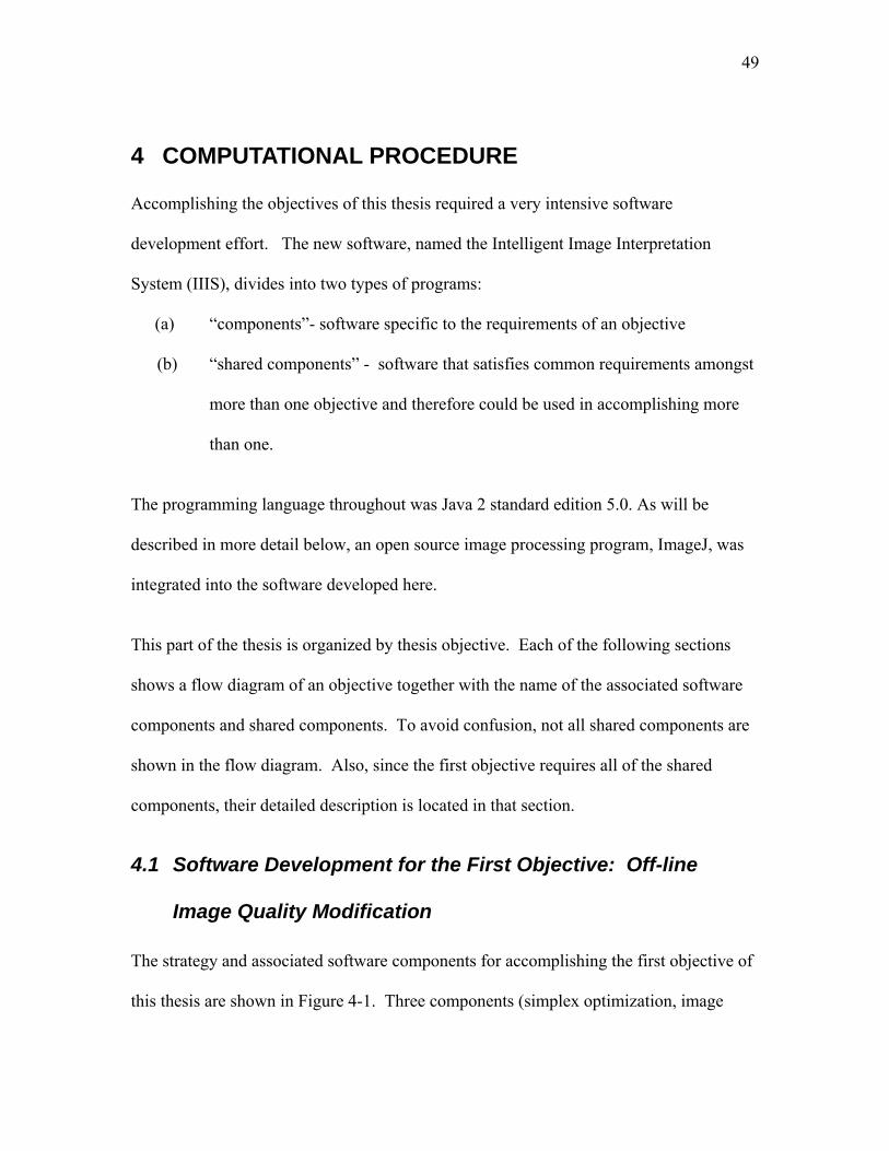
49
4 COMPUTATIONAL PROCEDURE Accomplishing the objectives of this thesis required a very intensive software
development effort. The new software, named the Intelligent Image Interpretation
System (IIIS), divides into two types of programs:
(a) “components”- software specific to the requirements of an objective
(b) “shared components” - software that satisfies common requirements amongst
more than one objective and therefore could be used in accomplishing more
than one.
The programming language throughout was Java 2 standard edition 5.0. As will be
described in more detail below, an open source image processing program, ImageJ, was
integrated into the software developed here.
This part of the thesis is organized by thesis objective. Each of the following sections
shows a flow diagram of an objective together with the name of the associated software
components and shared components. To avoid confusion, not all shared components are
shown in the flow diagram. Also, since the first objective requires all of the shared
components, their detailed description is located in that section.
4.1 Software Development for the First Objective: Off-line
Image Quality Modification
The strategy and associated software components for accomplishing the first objective of
this thesis are shown in Figure 4-1. Three components (simplex optimization, image
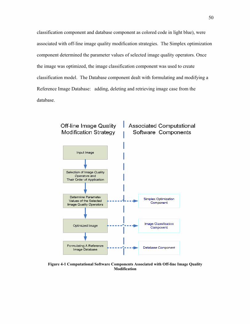
50
classification component and database component as colored code in light blue), were
associated with off-line image quality modification strategies. The Simplex optimization
component determined the parameter values of selected image quality operators. Once
the image was optimized, the image classification component was used to create
classification model. The Database component dealt with formulating and modifying a
Reference Image Database: adding, deleting and retrieving image case from the
database.
Figure 4-1 Computational Software Components Associated with Off-line Image Quality Modification

51
All software components involved in off-line image quality modification are discussed in
detail in the following subsections.
4.1.1 The Simplex Optimization Component
The Simplex optimization component is illustrated in Figure 4-2. The component is
enclosed with green dotted line. The grey boxes contain the steps required in the Simplex
optimization to determine the optimum parameter values of the selected image operators.
The blue boxes are software components associated with these steps. The steps required
in Simplex Optimization are image processing and objective function evaluation. The
image processing step modified the image with selected image quality operators whose
parameter values were “guessed” by the Simplex algorithm. The objective function
evaluation step assessed the performance of the image processing step. When the
optimization criterion was reached, the optimization stopped. At the same time, the
relevant information regarding the input image, including image quality metric values
and necessary attributes values of particle measurement as well as the IQ modification
instructions obtained in optimizing the image provided the image case, which was added
to the Reference Image Database by the database component.
In implementing the Simplex algorithm the parameter values guessed by the method were
constrained to physically realistic values by using a transformation from infinite space
(where the search was conducted) to parameter value space (where the parameter values
could possibly be). Further details on the Simplex method are provided in Appendix III.
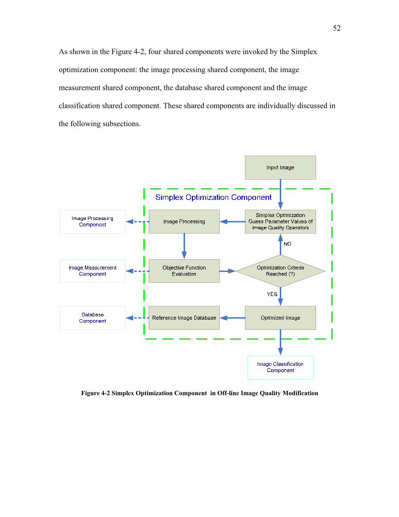
52
As shown in the Figure 4-2, four shared components were invoked by the Simplex
optimization component: the image processing shared component, the image
measurement shared component, the database shared component and the image
classification shared component. These shared components are individually discussed in
the following subsections.
Figure 4-2 Simplex Optimization Component in Off-line Image Quality Modification

53
4.1.2 The Image Processing Shared Component
In this work, the task of image processing was carried out by a free, open-source software
package (“ImageJ” available from http://rsb.info.nih.gov/ij/). All image quality
modification was done using Image J. Thus, as shown in Figure 4-3, the image
processing shared component is actually an interface to ImageJ. This component
combined image quality operators with their parameter values for processing and called
ImageJ to carry out the image modification task.
ImageJ contains 54 IQ operators for de-noising, blur removal, thresholding,
bright/contrast adjustment, edge sharpening, background flattening and other image
modification tasks. It also can provide a histogram of number of pixels versus their grey
level along with various statistics and particle related attributes.
Assembly Image Quality Operators and Their
parameters
Output Image
ProcessingCorresponding
ImageJProcessing Compoents
Image Processing
SharedComponent
Input Image
Figure 4-3 Image Processing Shared Component

54
In this work, “blanket preprocessing” of each raw image was performed previous to any
other modification. It included two operations: brightness adjustment to adjust the
average brightness to 128 and background flattening which corrected the non-uniformity
of illumination caused by uneven back lighting. Both operations were executed in
ImageJ. Similar blanket operations were carried out by Torabi in his work too. It’s a way
of reducing non-uniformity in image quality. After the raw image was blanket processed,
it was saved in an image folder for further processing.
The image processing shared component is a standalone component which was invoked
in both off-line and in-line image quality modification. The implementation of the image
processing component required a full understanding of ImageJ so that to allow access
some functions in ImageJ, which would otherwise be inaccessible. The major challenge
was to make such functions callable through macros from the image processing
component.
4.1.3 The Image Measurement Shared Component
The image measurement shared component (Figure 4-4) developed in this work served as
an interface to measurement (as opposed to image modification) functionalities in
ImageJ. This research involved many image measurement tasks, associated with image
quality metric measurement and particle related attribute measurement. The image
measurement shared component was frequently invoked by the simplex optimization
component and the case-based reasoning component.
ImageJ has 18 different measurements of particle attributes from an image. These
include particle area, mean grey value, standard deviation of grey value, max and min

55
grey value, etc. In this research, the measurements of interest were particle area and
particle mean grey value. The remainder of the measurements were not used.
Figure 4-4 Image Measurement Shared Component
As shown in Figure 4-4, the image measurement shared component first assembled the
measurement requirement. This could include an image quality metric for brightness,
contrast, noise, blur, illumination uniformity, and local contrast as well as attributes of
interested objects (particles). Depending on the type of measurement, different actions
would be taken. If the measurement was an IQ metric, the measurement tasks were
simply sent to ImageJ. In the case that the measurement was object (i.e. a particle)
related, first the image was thresholded using the image thresholding shared component;
then the measurement was performed using ImageJ.

56
However, ImageJ itself did not possess the capability to measure the six image quality
metrics: the brightness, contrast, noise, blur, illumination uniformity and local contrast.
Equations for these metrics are described in detail in Appendix II. These equations were
used by employing Image J to provide required variable values. The equations for
measuring illumination uniformity and local contrast were developed in this research
while the other four measurements were developed by other researchers.
4.1.4 The Image Thresholding Shared Component
The task of image thresholding is to separate the foreground objects of interest from the
background in order to extract relevant information about the objects of interest (particles
in this work). The image thresholding shared component (Figure 4-5) included a
modified version (termed Modified MaxMin thresholding) of Torabi’s MaxMin
thresholding (described in Section 2.2.2.1). The search for the required threshold value
started with setting an initial threshold value and then thresholding the image. The
thresholded image was then measured for particle attributes using ImageJ. If the
measurement reached the thresholding objective, that is, if the maximum minimum
particle size of the image was found, the thresholded image was output; otherwise the
threshold was systematically set at another value as described in Appendix IV and the
selection repeated until the desired threshold was located.
The modified version of MaxMin thresholding proved to be much more computationally
efficient (Appendix IV).

57
Set Threshold Value
Output Thresholded Image
ThresholdingImageJ Thresholding
Image ThresholdingShared Component
Input Image
Object/Particle Measurement
Thresholding ObjectiveReached (?)
ImageJ Object/Particle MeasurementComponent
YES
NO
Figure 4-5 Image Thresholding Shared Component
Like the image processing shared component, image thresholding shared component is a
standalone component which was used in both off-line and in-line image quality
modification. This shared component accessed the built-in ImageJ thresholding method
which sets the image background to white. Therefore, it had an interface to ImageJ.
4.1.5 The Image Classification Shared Component
The Bayesian classification model adopted in the work was implemented by the image
classification component (Figure 4-6). The model used here is essentially the same as that
developed in Torabi’s research as described in Section 2.2.2.2. The Bayesian model was
made adaptive by using the method described as the Intelligent Learning Machine (ILM)
(Appendix V).
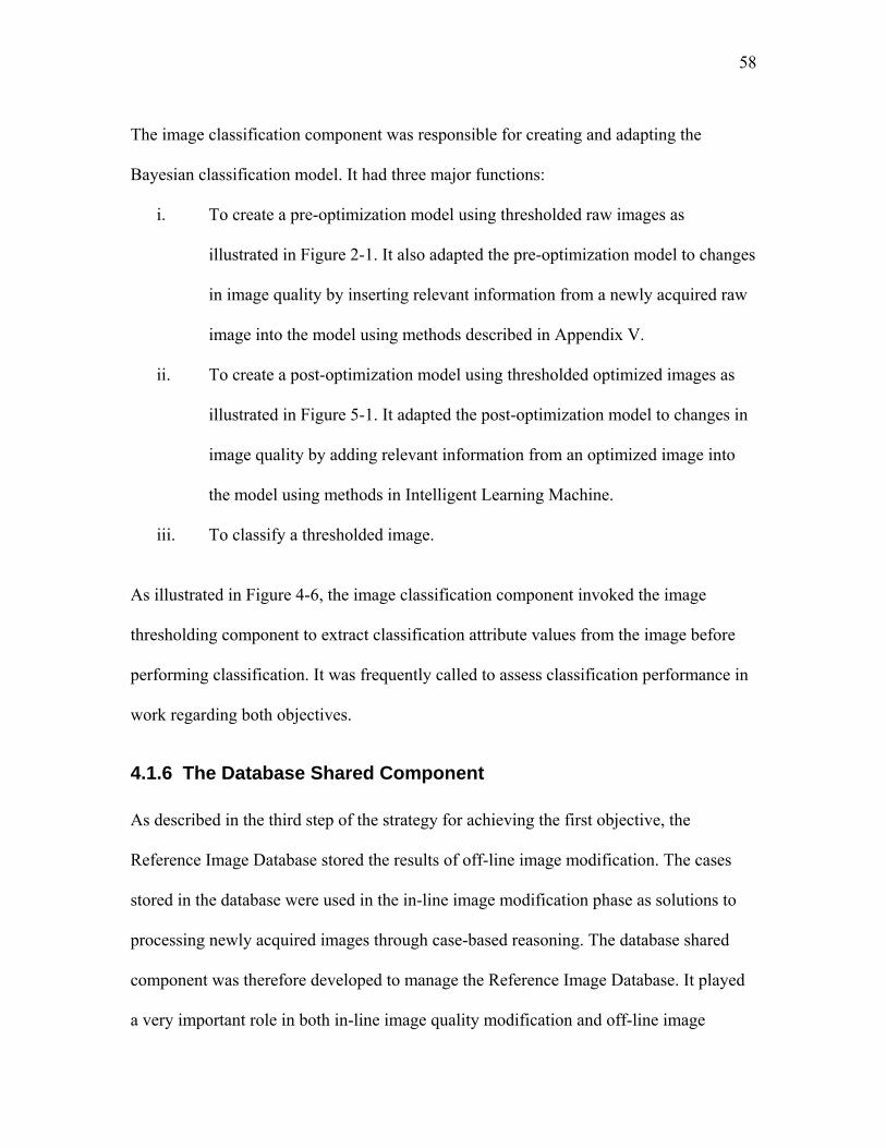
58
The image classification component was responsible for creating and adapting the
Bayesian classification model. It had three major functions:
i. To create a pre-optimization model using thresholded raw images as
illustrated in Figure 2-1. It also adapted the pre-optimization model to changes
in image quality by inserting relevant information from a newly acquired raw
image into the model using methods described in Appendix V.
ii. To create a post-optimization model using thresholded optimized images as
illustrated in Figure 5-1. It adapted the post-optimization model to changes in
image quality by adding relevant information from an optimized image into
the model using methods in Intelligent Learning Machine.
iii. To classify a thresholded image.
As illustrated in Figure 4-6, the image classification component invoked the image
thresholding component to extract classification attribute values from the image before
performing classification. It was frequently called to assess classification performance in
work regarding both objectives.
4.1.6 The Database Shared Component
As described in the third step of the strategy for achieving the first objective, the
Reference Image Database stored the results of off-line image modification. The cases
stored in the database were used in the in-line image modification phase as solutions to
processing newly acquired images through case-based reasoning. The database shared
component was therefore developed to manage the Reference Image Database. It played
a very important role in both in-line image quality modification and off-line image
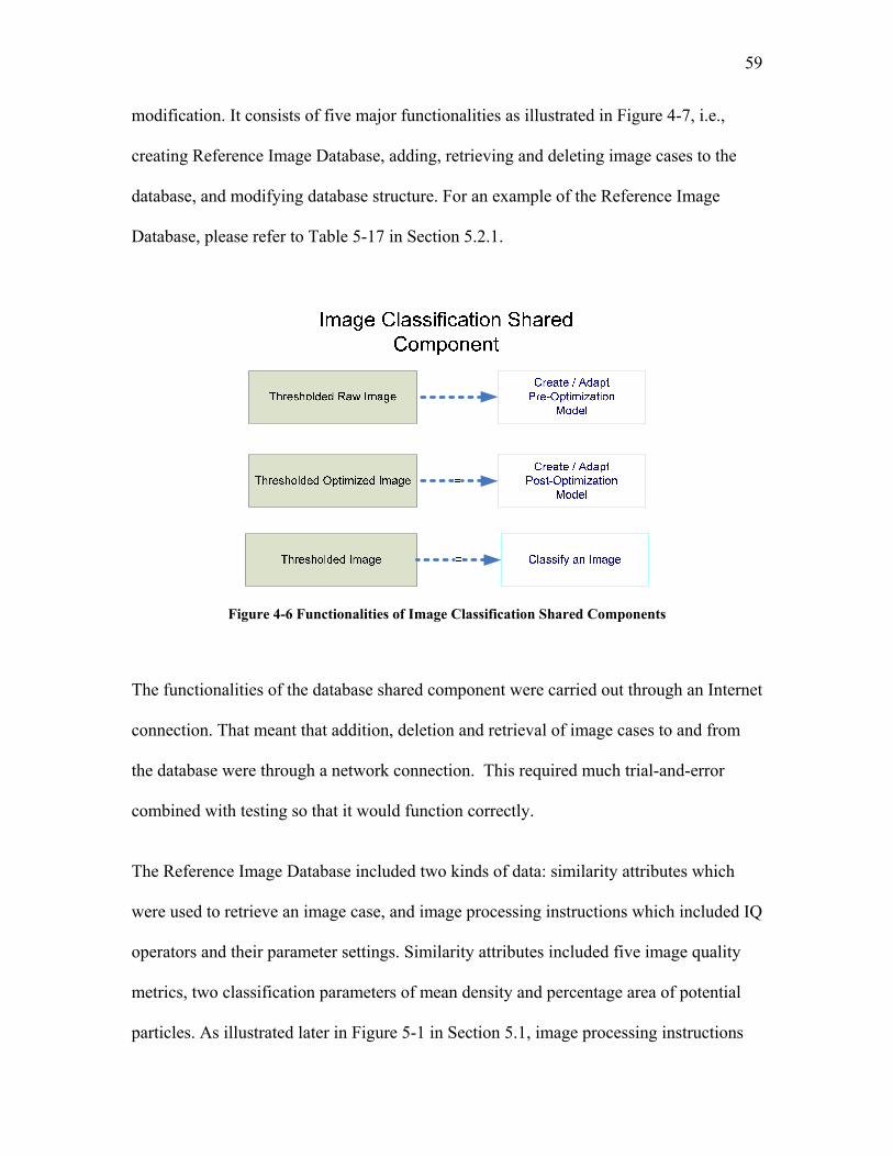
59
modification. It consists of five major functionalities as illustrated in Figure 4-7, i.e.,
creating Reference Image Database, adding, retrieving and deleting image cases to the
database, and modifying database structure. For an example of the Reference Image
Database, please refer to Table 5-17 in Section 5.2.1.
Figure 4-6 Functionalities of Image Classification Shared Components
The functionalities of the database shared component were carried out through an Internet
connection. That meant that addition, deletion and retrieval of image cases to and from
the database were through a network connection. This required much trial-and-error
combined with testing so that it would function correctly.
The Reference Image Database included two kinds of data: similarity attributes which
were used to retrieve an image case, and image processing instructions which included IQ
operators and their parameter settings. Similarity attributes included five image quality
metrics, two classification parameters of mean density and percentage area of potential
particles. As illustrated later in Figure 5-1 in Section 5.1, image processing instructions
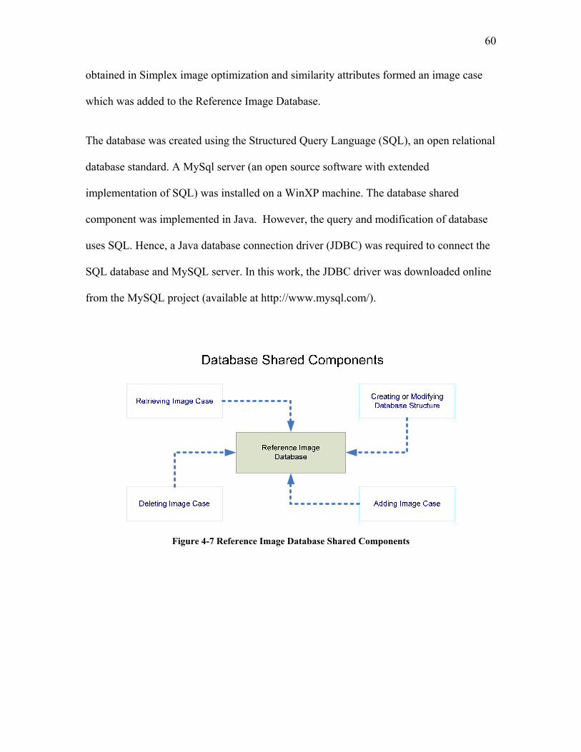
60
obtained in Simplex image optimization and similarity attributes formed an image case
which was added to the Reference Image Database.
The database was created using the Structured Query Language (SQL), an open relational
database standard. A MySql server (an open source software with extended
implementation of SQL) was installed on a WinXP machine. The database shared
component was implemented in Java. However, the query and modification of database
uses SQL. Hence, a Java database connection driver (JDBC) was required to connect the
SQL database and MySQL server. In this work, the JDBC driver was downloaded online
from the MySQL project (available at http://www.mysql.com/).
Figure 4-7 Reference Image Database Shared Components

61
4.2 Software Development for the Second Objective: In-line
Image Quality Modification
As described earlier, the objective of in-line image quality modification is to develop an
in-line method for modifying the quality of acquired images to permit improved
classification. The results of the first objective provide the required Reference Image
Database. The software components required to implement the strategies of achieving
this objective are shown in Figure 4-8. The left-hand side shows the strategy and the
right-hand side the software. Three major software components were necessary: the case-
based reasoning component, the image processing shared component and the image
classification shared component. The case-based reasoning component was developed to
locate the reference image in the Reference Image Database which most closely
resembled the newly acquired image. The associated image quality modification
instructions were then used to improve the quality of the newly acquired image by
employing the image processing component. The modified image was then classified by
the classification component.
The shared components mentioned were described above. The case-based reasoning
component is described below.

62
Figure 4-8 Computational Software Components Associated with In-line Image Quality Modification
The Case-based Reasoning Component
The case-based reasoning component (Figure 4-9) first measured the image quality
metrics and necessary attributes of particles of an image by invoking the image
measurement shared component. The measurement was then used by the database shared
component to locate the most similar image case in the Reference Image Database to the
current image case at hand. The IQ modification instructions associated with the retrieved
image case was then applied to process the current image using the image processing
shared component. The processed image was finally classified by the image classification
shared component. The classification result was compared to the class label previously

63
assigned by a human observer to determine whether it was correctly classified. If not, the
image was subjected to off-line image quality modification.
As can be seen, the computation involved in the case-based reasoning component of the
in-line image quality modification (the second objective) was not as complicated as that
in the Simplex optimization component which is the core component in off-line image
quality modification (the first objective). The reason is that it does not include the image
processing iterations and objective function evaluations which the Simplex optimization
component did.
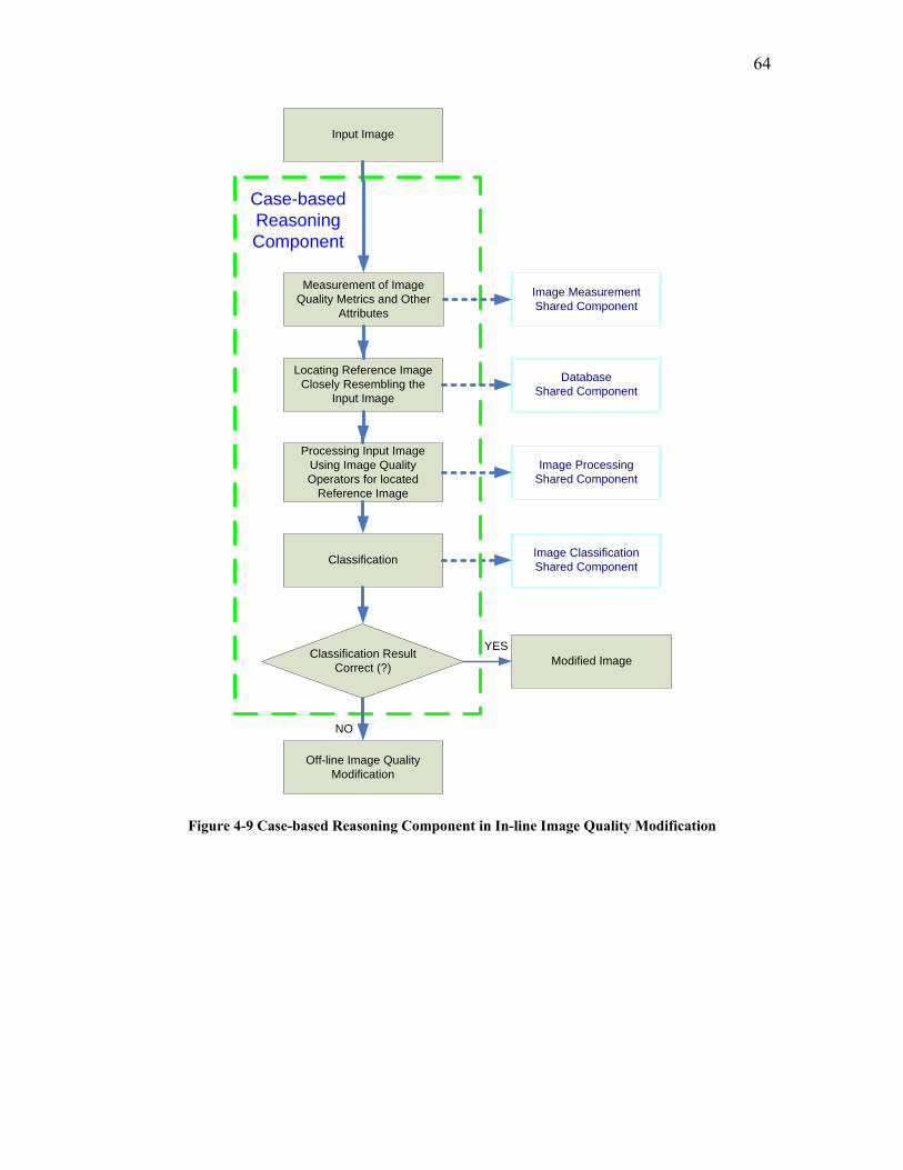
64
Locating Reference Image Closely Resembling the
Input Image
Classification
Off-line Image QualityModification
Processing Input ImageUsing Image Quality Operators for located
Reference Image
Classification ResultCorrect (?)
NO
Image ProcessingShared Component
Image ClassificationShared Component
Case-based Reasoning Component
Measurement of Image Quality Metrics and Other
Attributes
Input Image
Image MeasurementShared Component
DatabaseShared Component
Modified ImageYES
Figure 4-9 Case-based Reasoning Component in In-line Image Quality Modification

65
5 RESULTS AND DISCUSSION
5.1 Off-line Image Modification
This section shows results pertaining to the first objective of the thesis. Thus, it focuses
upon the development of an off-line automated method for obtaining the needed
improvement in image quality.
The work reported in this section uses “known” images. By that it meant that the class of
each image used has been determined in advance by a human observer and, most
importantly, the software is informed of the observer’s decision. It will be seen that this
is important to allowing a measure of image quality to be assigned. Also, when images
are used to create (i.e. train) a classification model then “known” images must be used.
In the usual training method, known as “cross-validation”, 90% of the images are known
and 10% are used for a testing step (the software is unaware of the human observer’s
classification for that 10%). The cross-validation training method uses ten trials wherein
it sequentially takes different images to constitute the 90% known images. Finally, the
results from the ten trials are averaged. In this thesis, “unknown images” are those for
which we know the result of the human observer classification but the software does not.
Thus, in the above description of cross-validation, the 10% of the data reserved for
testing in each trial would be considered as “unknown images” for that particular trial.
Figure 5-1 shows an overview of the system developed to accomplish the first objective
of this thesis: determining how to modify each individual raw image to the image quality
66
required for improved classification results. Beginning with the introduction of a raw
“known images” a pre-set blanket image processing operation is first carried out:
brightness is adjusted to a value of 128 and the background is flattened. This
“standardization” step is the same as that carried out by Torabi [33]. The objective
function is now used to assign an image quality value to the preprocessed image of an
input raw image. As compared to the approach in Torabi’s research as illustrated in
Figure 2-1, there is a crucial customized image quality modification step (as shown in
dotted box in Figure 5-1) developed prior to the creation of the classification model or
evaluation of the classification model.
Next the image is optimized using the Nelder-Mead Simplex optimization in order to
determine how to apply IQ Operators to transform it from a raw image to an image that
will be more successfully classified by the classification model. This involves:
i. Selecting the IQ Operators using some or all of the screens described in
Section 5.1.1.
ii. Systematically “guessing” the values of parameters in these operators.
iii. Applying the operators to the raw image
iv. Using the defined objective function to obtain the image quality.
v. Returning to step ii above until the image quality has been maximized.
Thus, at the conclusion of this procedure, for each raw image there is also an optimized
image. As will be seen later in this section, the most important results of this operation
are:
a. For the raw image:

67
i. values of the usual image characteristics (noise, blur, contrast, illumination
uniformity and brightness)
ii. values of mean particle density and percentage area.
iii. the value of image quality for the raw image.
iv. the identity of the image quality operators along with their parameter
values used to transform the raw image quality to the optimized image
quality.
b. For the optimized image:
i. the value of image quality for the optimized image.
ii. values of mean particle density and percentage area.
From the optimized images, values of mean particle density and percentage area were
extracted to create a post-optimization model, which could be later used for evaluating
the model and classifying test images in in-line image modification (“unknown images”).

68
Customized Image Quality Modification
Preprocessed Image
Simplex OptimizationGuess IQ Modifiers Parameter Values
Objective FunctionEvaluation
Optimized Image
Selection of IQ Modifiers and Determination of Their Order of Application
Image ProcessingIn ImageJ
Optimization CriteriaReached (?)
Added to Reference Image DatabaseWith optimum IQ Modifiers
Brightness AdjustmentAnd Background Flattening
NO
YES
Extracting Features
Modelling:Post-Optimization Model
Input Training Image
Evaluation:Classification
Figure 5-1 Off-line Image Quality Modification Framework

69
5.1.1 Selection of Image Quality Operators and their Order of Application
Reducing the dimensionality of the image quality modification problem is the first step in
accomplishing Objective 1. The dimension of the problem is extremely high due to the
fact that the number of the possible IQ Operators is large, the number of the order of their
application is large and, additionally, each IQ Operator has its own parameters.
A screening approach for dimension reduction was developed and depicted in Figure 5-2.
A major advantage of this approach is its generality. That is, it provides flexibility by
selecting IQ Operators, first based upon primary image characteristics and then upon task
specific criteria.
A sequence of screens is used, beginning with Screen 1 and concluding with Screen 3.
Each of these is described in turn in the following paragraphs along with the results
obtained.
5.1.1.1 Screen 1: Constraining Selection of IQ Operators by Selecting the Image Analysis Software
Screen 1 is image analysis software selection. Selection of the image analysis software
immediately introduces the first constraint by defining a set of IQ Operators which are
readily available. However, in addition to providing a suitable variety of IQ Operators
the software must be able to interface with other software to be used in the work. It also
must be economical and preferably open source (so that the actual workings of the image
analysis methods can be examined).
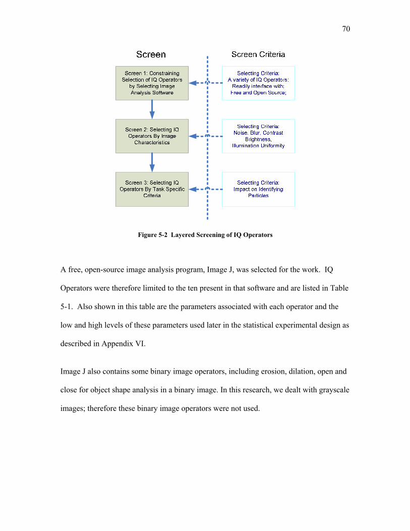
70
Figure 5-2 Layered Screening of IQ Operators
A free, open-source image analysis program, Image J, was selected for the work. IQ
Operators were therefore limited to the ten present in that software and are listed in Table
5-1. Also shown in this table are the parameters associated with each operator and the
low and high levels of these parameters used later in the statistical experimental design as
described in Appendix VI.
Image J also contains some binary image operators, including erosion, dilation, open and
close for object shape analysis in a binary image. In this research, we dealt with grayscale
images; therefore these binary image operators were not used.

71
Table 5-1 Image Quality Operators
Identifier Method Purpose Parameters Low Level
High Level
BR Brightness linear shift
Change the brightness Bias shift -σ +σ
CON Contrast stretch
Adjust the contrast Contrast gain
0.5 2
MN Mean filter Blur the active image Filter radius 1 4 SHP Sharpen Remove motion
induced or out-of-focus blur yet accentuates noises
Not applicable
0 1
EQL Histogram equalization
Enhance image contrast Not applicable
0 1
MD Median filter
Remove noise Filter radius 1 4
GB Gaussian Blur
Smooth the image Filter radius 1 4
GDIL Minimum grayscale dilation Filter radius 1 4 GER Maximum grayscale erosion Filter radius 1 4
Filter radius 1 4 UNSHP Unsharp mask
Sharpen & enhance edges Mask
Weight 0.2 0.9
SUB Subtract Background
Correct non-uniform illumination
Filter radius 20 50
Notes: 1) For image operators with lower level of 0 and high level 1, 0 represents the absence of the operator while 1 means the presence of the operator. 2) For method of brightness linear shift, σ is the standard deviation of image grey values.
5.1.1.2 Screen 2: Selection of IQ Operators by Image Characteristics From the literature review, it was evident that the vast majority of IQ Operators are
directed at changing only five image characteristics. These characteristics are: noise,
blur, contrast, illumination uniformity and brightness.

72
Screen 2 consists of qualitatively determining which each of these characteristics is
present in the image. The published literature can then provide guidance as to whether or
not a particular IQ Operator should be selected.
Dimension reduction is achieved by filtering out some unnecessary operators based on
the examination of the characteristics of a given image. Image characteristics are used to
determine what image processing tasks are needed to improve image quality. Image
processing tasks can involve using a single IQ Operator or a combination of IQ
Operators. These tasks include noise removal, edge sharpening, blur removal, contrast
enhancement, brightness adjustment, illumination correction and others. If there is a very
low noise level in the image, the task of noise removal is unnecessary. If noise presence
is strong, an appropriate operator for noise removal must be chosen. The choice of
operators for noise removal depends on the noise characteristics. If the noise is impulsive
(salt-and-pepper), then a median filter is an appropriate choice. If the noise is Gaussian,
then a Gaussian filter or mean filter is suitable. An overall strategy for qualitative pre-
selection of IQ Operators is illustrated in Figure 5-3 to Figure 5-7. Each of these figures
shows a “decision tree” for selection of IQ Operators to remedy noise, blur, contrast,
illumination and brightness.

73
Figure 5-3 Pre-selection of Image Operators for Noise Removal
Figure 5-4 Pre-selection of Image Operators for Blur Removal
Figure 5-5 Pre-selection of Image Operators for Contrast Enhancement
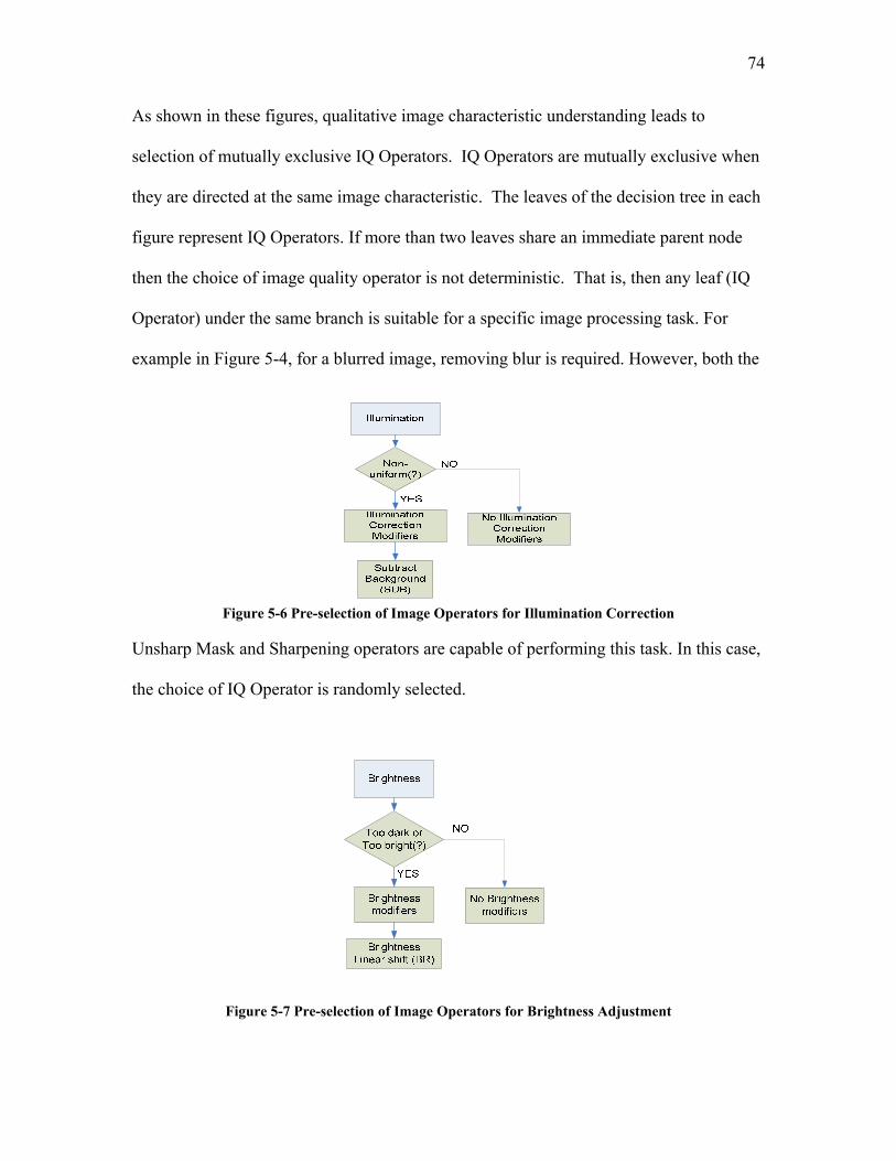
74
As shown in these figures, qualitative image characteristic understanding leads to
selection of mutually exclusive IQ Operators. IQ Operators are mutually exclusive when
they are directed at the same image characteristic. The leaves of the decision tree in each
figure represent IQ Operators. If more than two leaves share an immediate parent node
then the choice of image quality operator is not deterministic. That is, then any leaf (IQ
Operator) under the same branch is suitable for a specific image processing task. For
example in Figure 5-4, for a blurred image, removing blur is required. However, both the
Figure 5-6 Pre-selection of Image Operators for Illumination Correction
Unsharp Mask and Sharpening operators are capable of performing this task. In this case,
the choice of IQ Operator is randomly selected.
Figure 5-7 Pre-selection of Image Operators for Brightness Adjustment
75
In applying the decision trees of Figure 5-3 to 5-7 the following guidelines must be taken
into account:
i. Noise removal operators should precede sharpness operators. This can be justified
due to the fact that noise removal often causes blurring and sharpness operators
have a very strong tendency to magnify noise.
ii. The sharpening operator (SHP) is preferred over the unsharp mask (UNSHP) for
applications where small features (particles) are of interest because UNSHP in
general magnifies noise more than SHP.
iii. Contrast operators including contrast stretching (CON) and histogram equalization
(EQL) magnify noise. Thus noise removal operators should precede the contrast
operators.
iv. EQL tends to create artifacts which are difficult to remove by other image operators
particularly for images where noises are at the same grey level range as features.
Thus contrast stretching is preferred over EQL in this situation.
With the conclusion of Screen 2, the number of IQ Operators is reduced sufficiently to
allow closer examination of the remaining operators using task specific criteria.
The next section shows two examples of how Screen 2 was applied to images obtained by
the Scanning Particle Monitor.
5.1.1.3 The Application of Screen 2 to Images Obtained by the Scanning Particle Monitor
Screen 2: Example 1
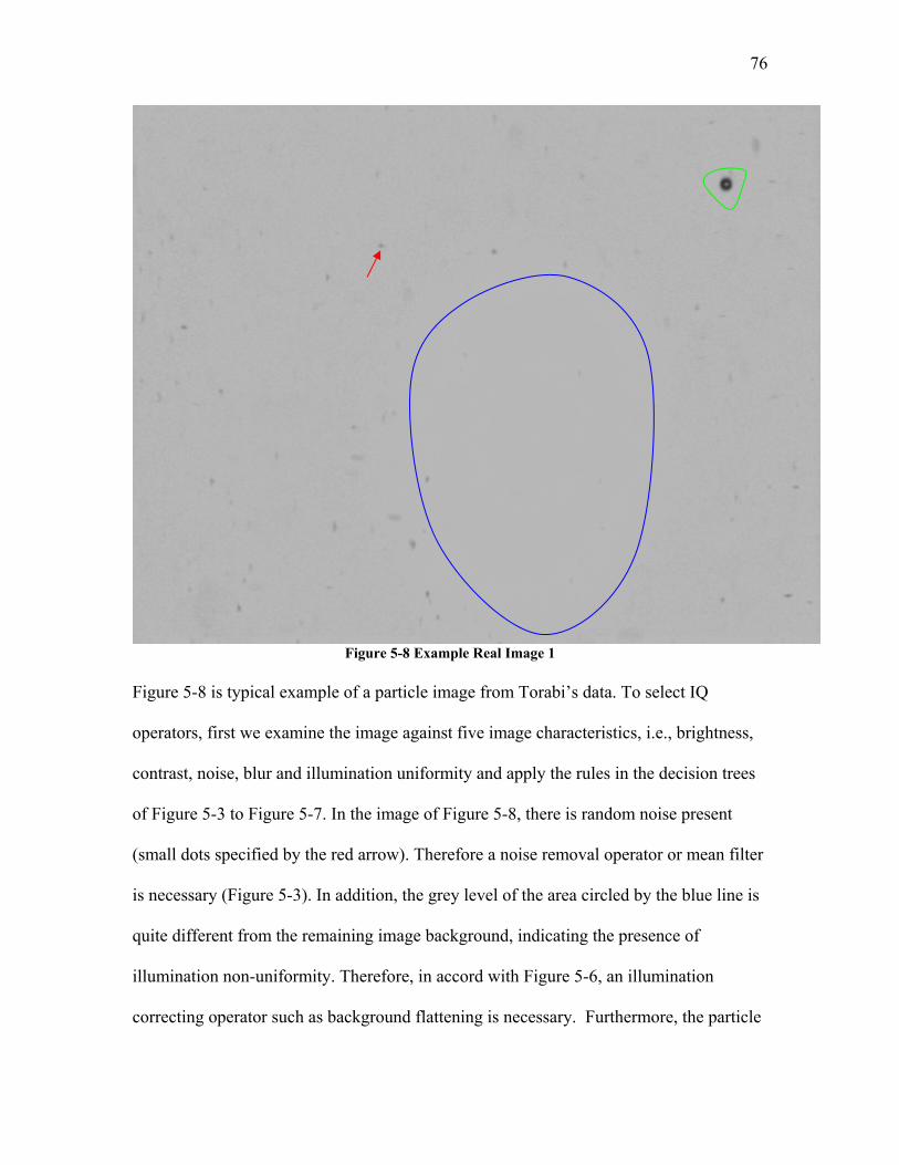
76
Figure 5-8 Example Real Image 1
Figure 5-8 is typical example of a particle image from Torabi’s data. To select IQ
operators, first we examine the image against five image characteristics, i.e., brightness,
contrast, noise, blur and illumination uniformity and apply the rules in the decision trees
of Figure 5-3 to Figure 5-7. In the image of Figure 5-8, there is random noise present
(small dots specified by the red arrow). Therefore a noise removal operator or mean filter
is necessary (Figure 5-3). In addition, the grey level of the area circled by the blue line is
quite different from the remaining image background, indicating the presence of
illumination non-uniformity. Therefore, in accord with Figure 5-6, an illumination
correcting operator such as background flattening is necessary. Furthermore, the particle

77
(circled in green) has a shiny center and also the image is quite bright, both of which
could be corrected by brightness adjustment (Figure 5-7). According to the guidelines
specified above, in terms of the order of application of IQ operators, brightness shift,
background flattening followed by mean filter would be the appropriate IQ operator
sequence to process the image.
Screen 2: Example 2
Figure 5-9 Example Real Image 2
The image of Figure 5-9 shows noise (specified by the red arrows) and blur around
particles (specified by the blue circles). Therefore, it is necessary to process the image
with the noise removal operator and a blur removal operator, i.e., mean filter and Sharpen

78
operator (Figure 5-3 and 5-4). In addition, the particles in the image have shining centers
and the image is too bright, both of which could be corrected by brightness adjustment to
make the image darker (Figure 5-7). Thus, in accord with the guidelines for Screen 2, this
image is to be processed by a brightness shift, mean filter and Sharpen operators in that
order.
5.1.1.4 Screen 3: Dimensionality Reduction: Selection of IQ Operators by Task Specific Criteria
In Screen 2, the IQ operators to improve IQ of an image are selected based on a set of
decision rules against five image quality characteristics. However, for computational
speed it is very desirable to further reduce the number of selected IQ operators if
possible. In this research, particle images are of the interest. The goal is to identify
particles in an image. Therefore, if the IQ operator has little or no effect on this goal then
it is reasonable to omit it. Initially a method involving test patterns and statistical
experimental designs was developed to systematically examine images. The method does
include some significant and novel contributions and so is described in Appendix VI.
However, in this work it served as a learning experience. From working to develop the
method a set of rules evolved to guide dimension reduction that provided a practical,
rapid solution. These rules are as follows:
i. If the noise present in the image is observed to be very small compared to the
particle image and has a much lower contrast to the background compared to
particle image, then the noise removal operator is unnecessary and could be
eliminated.

79
ii. An IQ Operator should not be eliminated if it is required by another operator.
That is, interaction effects amongst operators can be important. For example, in
the case of a noise removal operator such as a mean filter followed by blur
removal operator such as an Unsharp Mask, if the mean filter is eliminated, then
the Unsharp Mask will amplify the noise so much that the noise can be
misidentified as a particle. Therefore the mean filter should not be eliminated in
this situation.
To show how Screen 3 is applied we can return to the examples described for Screen 2.
For the image in Figure 5-8, in screen 2, it was decided that a sequence of background
flattening followed by mean filter be chosen. However, according to the decision rules
specified in Screen 3, the mean filter can be eliminated. That is because the size of the
particle present in the image is much greater than the noise and the grey level of the
particle is much lower than that of the noise (the noise grey level is very close to the
background grey level). Thus, the presence of noise would be unlikely to affect the
identification of the particle. By eliminating the mean filter, the sequence of IQ operators
could be abbreviated to brightness shift followed by background flattening.
In the second example, the image of Figure 5-9 as concluded for Screen 2, the image was
to be subjected to the image processing sequence of brightness shift, mean filter and
Sharpen operators. According to the second rule for Screen 3, this sequence cannot be
shortened because the elimination of mean filter will cause noise amplified by Sharpen
operators, therefore the sequence determined in Screen 2 will remain after the application
of Screen 3.
80
Each of the IQ operators selected by the screening process has variable parameters. The
value of the parameters is to be determined by optimizing image quality. However, first
a definition for image quality is necessary.
5.1.2 Image Quality Definition Once the IQ Operators and their order of application were identified according to the
method described above in Section 5.1.1, the next question was how best to use them for
each image in order to improve image quality for improved classification accuracy. A
method for determining the optimum parameter settings for each IQ Operator to achieve
image quality improvement was required. Therefore, a quantitative definition of image
quality was needed. The requirement actually was to characterize image quality with a
single number that would change as IQ Operators are applied to the image and that would
indicate how accurately the image can be classified as being WO (without particle) or
WP (with particle).
The four definitions of image quality examined in this work are now described in turn.
Following these descriptions, the improvement in classification results attained by using
each of them is compared.
The same set of images was used to evaluate each of the four definitions. These images
were randomly selected from images obtained in several different runs of in-line images
monitoring by Torabi. This set of images is a subset of Image Set 1 as listed in Table
3-1. In total, there are 745 images, of which 240 are “Without Particle (WO), and 505
“With Particle” (WP). These images are termed training images since they are labeled by

81
the human observer as WO or WP and the software is “told” of this classification. These
training images are used to create classification models.
5.1.2.1 Least Squares as Objective Function Image quality (IQ) can be summarized in a single number by using the same type of
“objective functions” as are minimized in non-linear regression. Here a weighted least
squares objective function compares the IQ Metric values of the image (Qi) with the
desired IQ Metric values (Qi,d):
∑=
−=5
1
2, )(
idii QQIQ 5-1
where Q1=noise, Q2= blur, Q3=contrast, Q4=illumination uniformity and Q5 = brightness).
The Qi values are measured from the image being considered. Calculation of the Qi
values is detailed in Appendix I. These quantities were all normalized so as to range
within [0,1] inclusive, with zero being the worst and unity being the best for each
individual metric. Qi,d is the value of Qi desired for the image, and the Qi,d values by
definition are unity for all five IQ metrics.
In this subsection, the application of Least Squares (LS) as objective function and its
impact on classification is discussed in details. Furthermore, its relationship with
classification results will be examined to determine if there is a positive correlation
between Lease Squares image quality and classification.
Classification Results Using Least Squares as Objective Function
To provide “baseline values” for classifier performance in this section of the thesis, raw
(not optimized) images were classified using the Torabi Bayesian model. Actually, the
82
model used has a modified thresholding method described in Appendix IV. The
confusion matrix for the classification is shown in Table 5-2, where of the 505 images
that actually contained particles (were in class WP), 489 of them were correctly predicted
(true positives) and 16 of them were incorrectly predicted as having no particles (false
negatives). For the evaluation of classification methods and all related terminology,
please refer to Section 2.5 in the literature review. Of the 240 images that did actually
not contain any particles, 25 of them were incorrectly predicted as having particles (false
positives) and 215 of them were correctly predicted as having no particles. This number
of false positives is 10.4% of the number of images that actually have no particles (i.e. a
false positive rate of 10.4%) and would be responsible for many false alarms in a
classification operation. The number of false negatives is 3.2% of the total number of
images that actually do have a particle and could allow the production of considerable
off-spec product. The overall classification accuracy calculated based on Table 5-2 is a
respectable 94.5 %. However, this can also be viewed as a classification error of 5.5% as
shown in Figure 5-10. That is, if no customized image processing is done then about one
in every twenty images is misclassified.
Table 5-3 shows the classification confusion matrix of images optimized using the
unweighted least squares (LS) objective function and Figure 5-10 compares the
classification error rate, false positive rate and false negative rate with the classification
of the raw images mentioned above. Error rates are compared using bar charts as in
Figure 5-10. The 95% confidence interval for each error rate is marked at the top of each
bar. Appendix IX shows an example calculation for the 95% confidence interval. The
data labels on the top of each bar are the calculated error rate from confusion matrix.

83
As shown in Figure 5-10, the classification of raw images yields an overall 94.5%
accuracy while that of Least Squares optimized images yields an overall 98.2% accuracy.
3.7% rise in accuracy between raw image and Least Squares optimized images is
considered a significant improvement. The false positive rate 10.4% for the model based
on raw images is unacceptable. In contrast, the model based on Least Squares optimized
image is able to achieve a balanced true positive rate (98.6%) and false positive rate
(2.5% or true negative rate of 97.5%).
Table 5-2 Classification Confusion Matrix for the Training Set of Raw Images
Table 5-3 Classification Confusion Matrix for the Training Set of Images Optimized Using the Least
Squares Objective Function
Predicted Class is WP Predicted Class is WO Actual Class is WP 489 16 Actual Class is WO 25 215
Predicted Class is WP Predicted Class is WO Actual Class is WP 498 7 Actual Class is WO 6 234
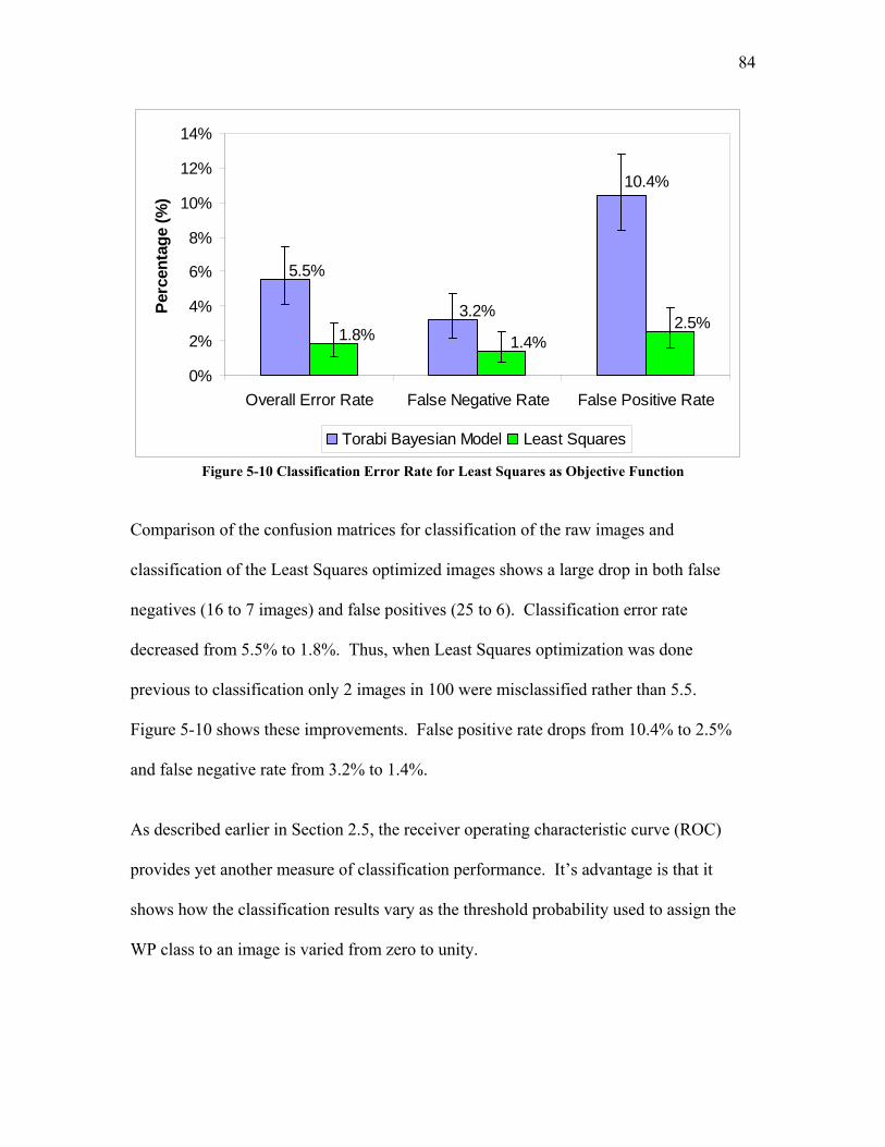
84
10.4%
3.2%
5.5%
2.5%1.8% 1.4%
0%
2%
4%
6%
8%
10%
12%
14%
Overall Error Rate False Negative Rate False Positive Rate
Perc
enta
ge (%
)
Torabi Bayesian Model Least Squares
Figure 5-10 Classification Error Rate for Least Squares as Objective Function Comparison of the confusion matrices for classification of the raw images and
classification of the Least Squares optimized images shows a large drop in both false
negatives (16 to 7 images) and false positives (25 to 6). Classification error rate
decreased from 5.5% to 1.8%. Thus, when Least Squares optimization was done
previous to classification only 2 images in 100 were misclassified rather than 5.5.
Figure 5-10 shows these improvements. False positive rate drops from 10.4% to 2.5%
and false negative rate from 3.2% to 1.4%.
As described earlier in Section 2.5, the receiver operating characteristic curve (ROC)
provides yet another measure of classification performance. It’s advantage is that it
shows how the classification results vary as the threshold probability used to assign the
WP class to an image is varied from zero to unity.

85
In Figure 5-11 there are two ROC curves for Least Squares and model of raw images,
respectively (note that parts of ROC curves for the model of raw images are
superimposed by the ROC curve for the Least Squares optimized images). The
classification accuracies for raw and Least Squares optimized images listed in Figure
5-10 are two data points on the corresponding ROC curve (as shown in Figure 5-11).
The ROC curve for the Least Squares optimized images is far superior to that for the raw
images because it is always to the left and above the ROC curve for classification of raw
images.
0
0.1
0.2
0.3
0.4
0.5
0.6
0.7
0.8
0.9
1
0 0.2 0.4 0.6 0.8 1False Positive Rate
True
Pos
itive
Rat
e
Bayesian Model of Raw ImagesBayesian Model of Least Squares Optimized Images
Maximum Accuracyfor Bayesian Model of Raw Images
Maximum Accuracyfor Bayesian Model of Lease SquaresOptimized Images
12
Figure 5-11 ROC Curve for Least Squares as Objective Function

86
As mentioned previously, the Area Under a ROC curve (AUC) provides a useful measure
of the general superiority of one classifier over another because it includes consideration
of more than the overall classification error rate. The AUCs are 0.974 and 0.998 for
classifiers of raw images and Least Squares optimized images. As expected, from the
appearance of the curves in Figure 5-11, the AUC for classification of images optimized
using a Least Squares objective function is significantly larger than that of the raw
images.
The training image set used here have a skewed class distribution of 1:2 (WO: WP). In
this situation, ROC analysis suggests that the optimal operating point on the ROC curve
be the one at which the tangent of the curve is 1/2.
Relationship between Least Squares as Objective Function and Classification Results These results were very promising. However, since even better results were desired, an
effort was initiated to determine how best to improve the least squares objective function
definition of image quality. Table 5-4 shows the average Least Squares image quality
values for the raw images and for the Least Squares optimized images (correctly and
then, incorrectly classified images) along with their respective 95% confidence intervals.
As expected, the average image quality of the Least Squares optimized images is
significantly greater than the raw images (0.616 versus 0.335). However, surprisingly,
there was no significant difference between the average image quality of the correctly
and incorrectly classified Least Squares optimized images (0.617 and 0.584 respectively).
To further assess the IQ definition, the IQ values of each individual image was examined
(rather than only the average values). Figure 5-12 is a plot of Image Quality (i.e. the
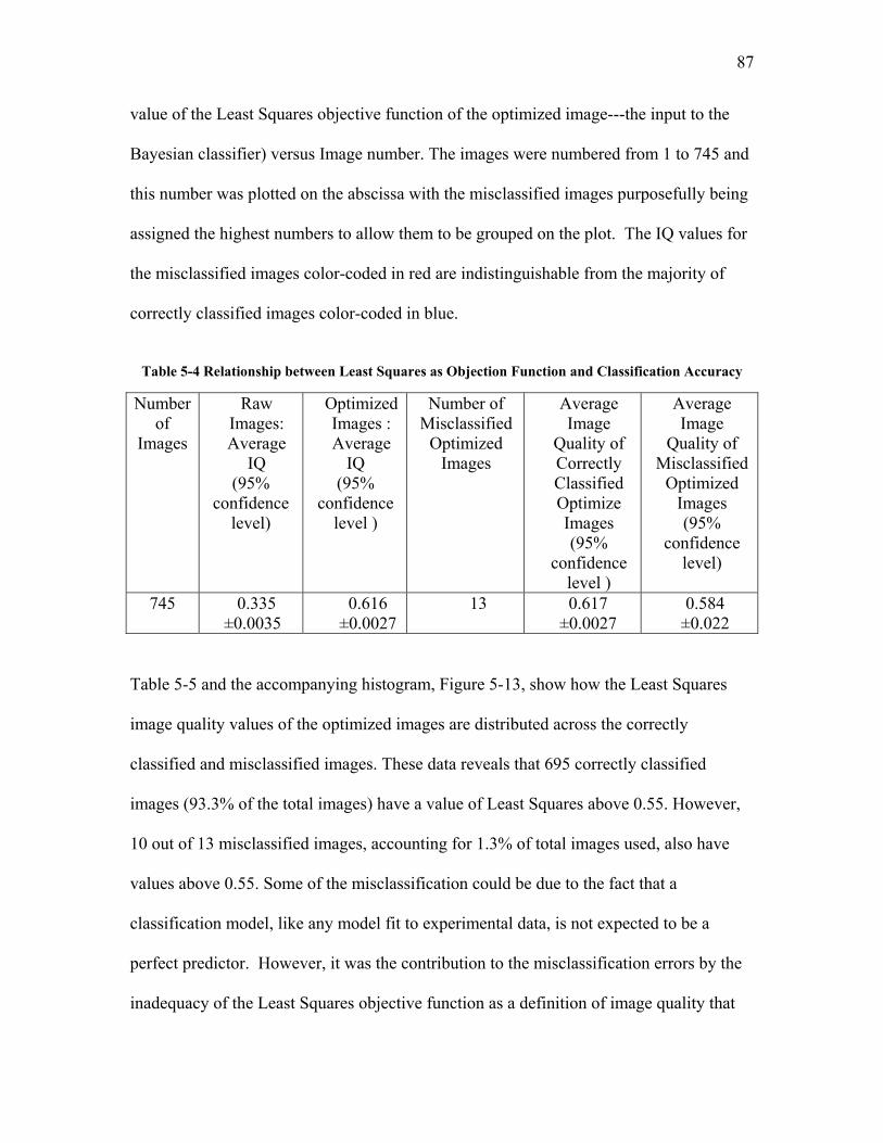
87
value of the Least Squares objective function of the optimized image---the input to the
Bayesian classifier) versus Image number. The images were numbered from 1 to 745 and
this number was plotted on the abscissa with the misclassified images purposefully being
assigned the highest numbers to allow them to be grouped on the plot. The IQ values for
the misclassified images color-coded in red are indistinguishable from the majority of
correctly classified images color-coded in blue.
Table 5-4 Relationship between Least Squares as Objection Function and Classification Accuracy
Table 5-5 and the accompanying histogram, Figure 5-13, show how the Least Squares
image quality values of the optimized images are distributed across the correctly
classified and misclassified images. These data reveals that 695 correctly classified
images (93.3% of the total images) have a value of Least Squares above 0.55. However,
10 out of 13 misclassified images, accounting for 1.3% of total images used, also have
values above 0.55. Some of the misclassification could be due to the fact that a
classification model, like any model fit to experimental data, is not expected to be a
perfect predictor. However, it was the contribution to the misclassification errors by the
inadequacy of the Least Squares objective function as a definition of image quality that
Number of
Images
Raw Images: Average
IQ (95%
confidence level)
Optimized Images : Average
IQ (95%
confidence level )
Number of Misclassified
Optimized Images
Average Image
Quality of Correctly Classified Optimize Images (95%
confidence level )
Average Image
Quality of Misclassified
Optimized Images (95%
confidence level)
745 0.335 ±0.0035
0.616 ±0.0027
13 0.617 ±0.0027
0.584 ±0.022
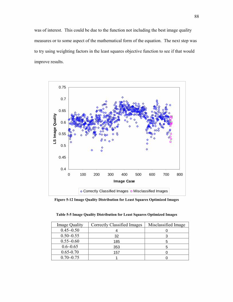
88
was of interest. This could be due to the function not including the best image quality
measures or to some aspect of the mathematical form of the equation. The next step was
to try using weighting factors in the least squares objective function to see if that would
improve results.
0.4
0.45
0.5
0.55
0.6
0.65
0.7
0.75
0 100 200 300 400 500 600 700 800
Image Case
LS Im
age
Qua
lity
Correctly Classified Images Misclassified Images
Figure 5-12 Image Quality Distribution for Least Squares Optimized Images
Table 5-5 Image Quality Distribution for Least Squares Optimized Images
Image Quality Correctly Classified Images Misclassified Image 0.45~0.50 4 0 0.50~0.55 32 3 0.55~0.60 185 5 0.6~0.65 353 5 0.65-0.70 157 0 0.70~0.75 1 0

89
32
185
353
157
4 1
0 0
0
5
5
3
0
50
100
150
200
250
300
350
400
0.45-0.5 0.5-0.55 0.55-0.6 0.6-0.65 0.65-0.7 0.7-0.75
LS Image Quality
Num
ber o
f Im
ages
Correctly Classified Images Misclassified Images
Figure 5-13 Image Quality Histogram for Least Squares Optimized Images
5.1.2.2 Weighted Least Squares (WLS) as Objective Function With the introduction of weighting factors the least squares objective function (Equation
5.1) becomes a weighted least squares objective function:
∑=
−=5
1
2, )(
idiii QQwIQ 5-2
where Q1=noise, Q2= blur, Q3=contrast, Q4=illumination uniformity and Q5 = brightness)
and wi are “weighting factors” that serve to provide the relative importance of a
particular metric difference to the IQ value.
The weighting factors were obtained from:
ri
LSirii Q
QQw
,
,, || −= 5-3
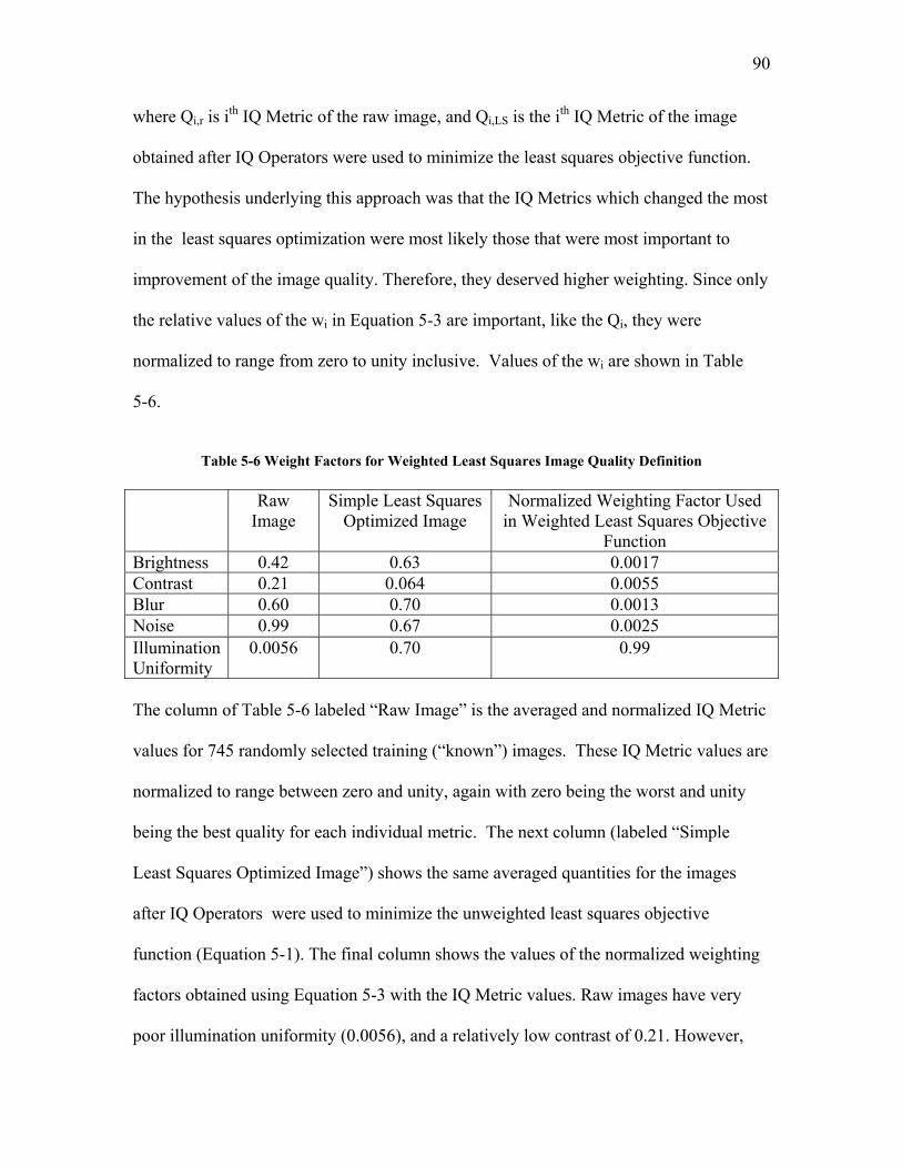
90
where Qi,r is ith IQ Metric of the raw image, and Qi,LS is the ith IQ Metric of the image
obtained after IQ Operators were used to minimize the least squares objective function.
The hypothesis underlying this approach was that the IQ Metrics which changed the most
in the least squares optimization were most likely those that were most important to
improvement of the image quality. Therefore, they deserved higher weighting. Since only
the relative values of the wi in Equation 5-3 are important, like the Qi, they were
normalized to range from zero to unity inclusive. Values of the wi are shown in Table
5-6.
Table 5-6 Weight Factors for Weighted Least Squares Image Quality Definition
Raw
Image Simple Least Squares
Optimized Image Normalized Weighting Factor Used
in Weighted Least Squares Objective Function
Brightness 0.42 0.63 0.0017 Contrast 0.21 0.064 0.0055 Blur 0.60 0.70 0.0013 Noise 0.99 0.67 0.0025 Illumination Uniformity
0.0056 0.70 0.99
The column of Table 5-6 labeled “Raw Image” is the averaged and normalized IQ Metric
values for 745 randomly selected training (“known”) images. These IQ Metric values are
normalized to range between zero and unity, again with zero being the worst and unity
being the best quality for each individual metric. The next column (labeled “Simple
Least Squares Optimized Image”) shows the same averaged quantities for the images
after IQ Operators were used to minimize the unweighted least squares objective
function (Equation 5-1). The final column shows the values of the normalized weighting
factors obtained using Equation 5-3 with the IQ Metric values. Raw images have very
poor illumination uniformity (0.0056), and a relatively low contrast of 0.21. However,

91
their noise level is low with a value of 0.99 (For noise, blur and illumination uniformity
metrics, a larger value means less noise, less blur and high illumination uniformity and
vice versa). With a weighting of 0.99, Illumination Uniformity was of overwhelming
importance to image quality compared to the other image characteristics. Contrast and
noise of the images optimized using simple least squares surprisingly became worse than
those of the raw image.
Classification Results Using Weighted Least Squares as the Objective Function Table 5-7 shows the confusion matrix for classification of the images using the weighted
least squares objective function as the definition of image quality. Figure 5-14 shows the
classification errors in comparison to the classification of raw images. In comparison
with the results using raw images (Table 5-2) there was a significant improvement as
shown in Figure 5-14. However, in comparison with the unweighted least squares
objective function (Table 5-3 and Figure 5-10) there is no significant improvement.
Table 5-7 Confusion Matrix for Weighted Least Squares Optimized Images
Predicted Class is WP Predicted Class is WO Actual Class is WP 499 6 Actual Class is WO 8 232
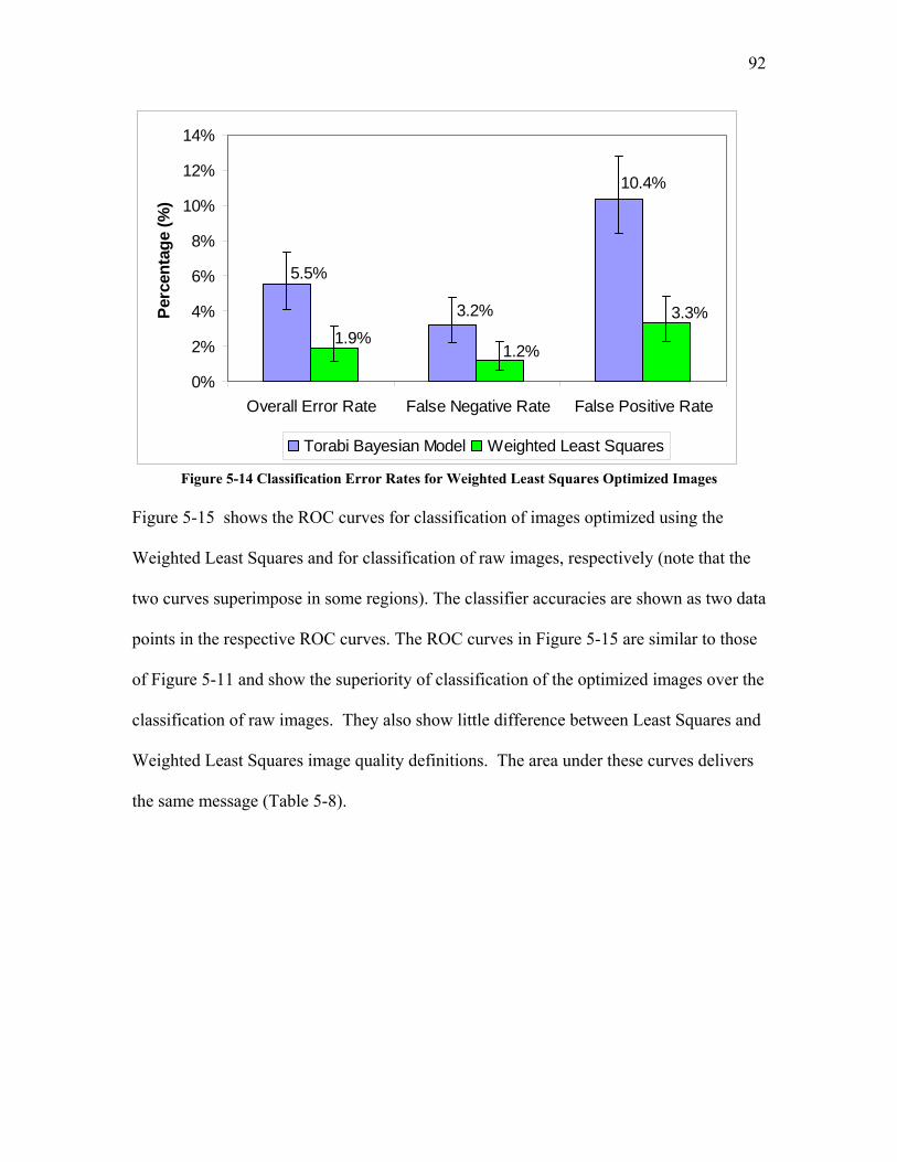
92
10.4%
5.5%
3.2% 3.3%
1.2%1.9%
0%
2%
4%
6%
8%
10%
12%
14%
Overall Error Rate False Negative Rate False Positive Rate
Perc
enta
ge (%
)
Torabi Bayesian Model Weighted Least Squares
Figure 5-14 Classification Error Rates for Weighted Least Squares Optimized Images Figure 5-15 shows the ROC curves for classification of images optimized using the
Weighted Least Squares and for classification of raw images, respectively (note that the
two curves superimpose in some regions). The classifier accuracies are shown as two data
points in the respective ROC curves. The ROC curves in Figure 5-15 are similar to those
of Figure 5-11 and show the superiority of classification of the optimized images over the
classification of raw images. They also show little difference between Least Squares and
Weighted Least Squares image quality definitions. The area under these curves delivers
the same message (Table 5-8).
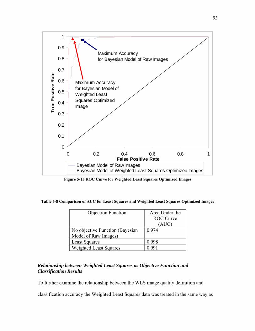
93
0
0.1
0.2
0.3
0.4
0.5
0.6
0.7
0.8
0.9
1
0 0.2 0.4 0.6 0.8 1False Positive Rate
True
Pos
itive
Rat
e
Bayesian Model of Raw ImagesBayesian Model of Weighted Least Squares Optimized Images
Maximum Accuracyfor Bayesian Model of Raw Images
Maximum Accuracyfor Bayesian Model of Weighted LeastSquares Optimized Image
Figure 5-15 ROC Curve for Weighted Least Squares Optimized Images
Table 5-8 Comparison of AUC for Least Squares and Weighted Least Squares Optimized Images
Objection Function Area Under the
ROC Curve (AUC)
No objective Function (Bayesian Model of Raw Images)
0.974
Least Squares 0.998 Weighted Least Squares 0.991
Relationship between Weighted Least Squares as Objective Function and Classification Results To further examine the relationship between the WLS image quality definition and
classification accuracy the Weighted Least Squares data was treated in the same way as

94
the Least Squares data. Table 5-9 shows the average values of Weighted Least Squares
image quality and Figure 5-16 shows a plot of image quality versus image number. The
overall classification error rate as shown in Figure 5-14 was very similar to that obtained
as shown in Figure 5-10 for the simple least squares definition of image quality. Thus,
the Weighted Least Squares image quality definition did not really provide an
improvement in classification performance over unweighted least squares.
Table 5-9 Relationship between Weighted Least Squares as Objection Function and Classification
Accuracy
Number of
Images
Raw Images: Average IQ( 95%
confidence Level)
Optimized Images:
Average IQ (95%
confidence level)
Number of Misclassified Optimized
Images
Average Image
Quality of Correctly Classified Optimize Images (95%
confidence level)
Average Image
Quality of Misclassified
Optimized Images (95%
confidence level)
745 0.335 ±0.0035
0.766 ±0.0073
14 0.765 ±0.0074
0.824 ±0.027
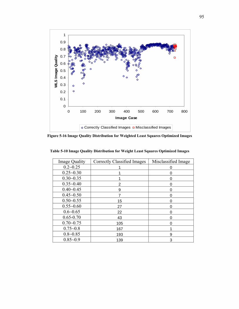
95
0
0.1
0.2
0.3
0.4
0.5
0.6
0.7
0.8
0.9
1
0 100 200 300 400 500 600 700 800
Image Case
WLS
Imag
e Q
ualit
y
Correctly Classified Images Misclassified Images
Figure 5-16 Image Quality Distribution for Weighted Least Squares Optimized Images
Table 5-10 Image Quality Distribution for Weight Least Squares Optimized Images
Image Quality Correctly Classified Images Misclassified Image 0.2~0.25 1 0 0.25~0.30 1 0 0.30~0.35 1 0 0.35~0.40 2 0 0.40~0.45 9 0 0.45~0.50 7 0 0.50~0.55 15 0 0.55~0.60 27 0 0.6~0.65 22 0 0.65-0.70 43 0 0.70~0.75 105 0 0.75~0.8 167 1 0.8~0.85 193 9 0.85~0.9 139 3

96
0
50
100
150
200
250
0.2-0.
25
0.25-0
.3
0.3-0.
35
0.35-0
.4
0.4-0.
45
0.45-0
.5
0.5-0.
55
0.55-0
.6
0.60-0
.65
0.65-0
.7
0.7-0.
75
0.75-0
.8
0.8-0.
85
0.85-0
.9
WLS Image Quality
Num
ber o
f Im
ages
Correctly Classified Misclassified
Figure 5-17 Image Quality Histogram for Weighted Least Squares Optimized Images Thus, at this point it was evident that using a simple or a weighted least squares objective
function to define image quality provided improvement in image classification over
classification of raw images. However, to improve classification results still more it was
thought that perhaps a better objective function would be the one that prevented any
individual IQ Metric value from being forced into extremely low values. That led to
consideration of the “desirability function”.
5.1.2.3 The Desirability Function as Objective Function The desirability function is defined as:
nQQQQQIQ /154321 )( ××××= 5-4
where Q1, Q2, Q3, Q4, Q5 are five IQ Metrics defined, parameter n is a constant power. In
this research, n is set to 1. Therefore, the definition becomes the product of five IQ
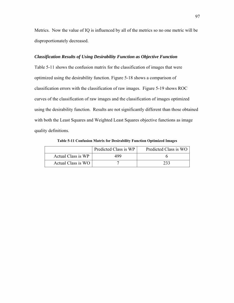
97
Metrics. Now the value of IQ is influenced by all of the metrics so no one metric will be
disproportionately decreased.
Classification Results of Using Desirability Function as Objective Function Table 5-11 shows the confusion matrix for the classification of images that were
optimized using the desirability function. Figure 5-18 shows a comparison of
classification errors with the classification of raw images. Figure 5-19 shows ROC
curves of the classification of raw images and the classification of images optimized
using the desirability function. Results are not significantly different than those obtained
with both the Least Squares and Weighted Least Squares objective functions as image
quality definitions.
Table 5-11 Confusion Matrix for Desirability Function Optimized Images
Predicted Class is WP Predicted Class is WO Actual Class is WP 499 6 Actual Class is WO 7 233

98
10.4%
5.5%
3.2% 2.9%
1.2%1.8%
0%
2%
4%
6%
8%
10%
12%
14%
Overall Error Rate False Negative Rate False Positive Rate
Perc
enta
ge (%
)
Torabi Bayesian Model Desirability Function
Figure 5-18 Classification Error Rate for Desirability Function Optimized Images
00.10.20.30.40.50.60.70.80.9
1
0 0.2 0.4 0.6 0.8 1False Positive Rate
True
Pos
itive
Rat
e
Bayesian Model of Raw ImagesBayesian Model of Desirability Function Optimized Images
Figure 5-19 ROC Curve for Desirability Function Optimized Images
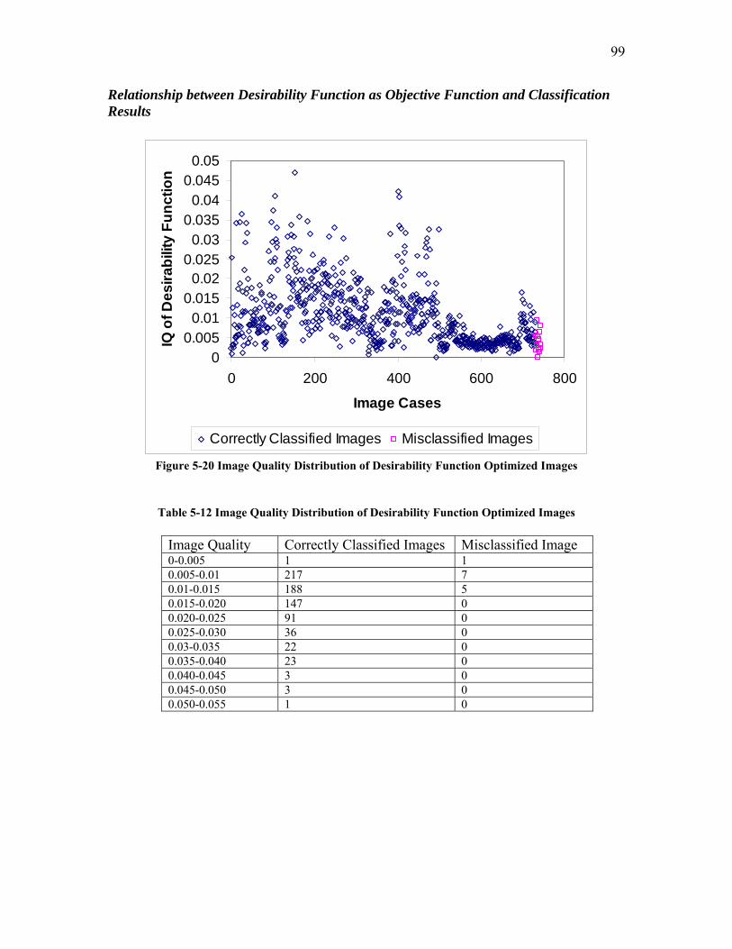
99
Relationship between Desirability Function as Objective Function and Classification Results
00.005
0.010.015
0.020.025
0.030.035
0.040.045
0.05
0 200 400 600 800
Image Cases
IQ o
f Des
irabi
lity
Func
tion
Correctly Classified Images Misclassified Images
Figure 5-20 Image Quality Distribution of Desirability Function Optimized Images
Table 5-12 Image Quality Distribution of Desirability Function Optimized Images
Image Quality Correctly Classified Images Misclassified Image 0-0.005 1 1 0.005-0.01 217 7 0.01-0.015 188 5 0.015-0.020 147 0 0.020-0.025 91 0 0.025-0.030 36 0 0.03-0.035 22 0 0.035-0.040 23 0 0.040-0.045 3 0 0.045-0.050 3 0 0.050-0.055 1 0

100
0
50
100
150
200
250
0 0.005 0.01 0.015 0.02 0.025 0.03 0.035 0.04 0.045 0.05
IQ of Desirability Function
Num
ber o
f Im
ages
Correctly Classified Images Misclassified Images
Figure 5-21 Image Quality Histogram for Desirability Function Optimized Images
Experience with the weighted least squares objective function and the desirability
function led to the hypothesis that to obtain further image quality improvement for
classification the definition of image quality had to be more directly linked with the
classification model. This was done by using the classification model itself to formulate
a definition for image quality and is described in the next section.
5.1.2.4 Probability Density Difference as Objective Function Classification of the images into WO and WP in this work is carried out using a Bayesian
classification model (explained in Section 2.2.2.2 in the thesis). The model was
previously developed by Torabi. In Section 2.2.2.2 it was mentioned that the input to this
model is percentage area of the particles and mean density of the particles. In contrast,
the image quality functions described above use image characteristics more commonly

101
found in the image processing literature (noise, blur, contrast, illumination uniformity and
brightness). Thus, one way of improving the link between the image quality definition
and the classification accuracy would be to replace the literature image quality
characteristics with those actually used for classification in Equation 2-8. However, the
uncertainties associated with how best to assign the values of weighting factors and even
the exact form of the objective function would then still remain. Instead, an image
quality definition that was based upon using the same type of classification model to
obtain a measure of image quality was devised. That meant dealing with two
classification models. One (termed the “pre-optimization model”) is used to characterize
image quality of images that have previously been assigned to a WO or WP class by a
human observer (i.e. it is used only to assign an image quality number to a “known”
image). This model is created the same way as in Torabi’s research (Figure 2-1). The
second, and formerly the only model used, was termed the “post-optimization model” and
was used to classify “unknown” images as WO or WP. Its creation is illustrated in Figure
5-1.
As described earlier (Section 2.2.2.2), in conventional data mining practice the Bayesian
model utilizes the calculation of probability densities for the attribute values. More
specifically, the value of f(X=x|C=WP)P(C=WP) is compared to the value of
f(X=x|C=WO)P(C=WO) for an image and the image is classified as WP or WO
depending upon whether the former or latter quantity is the greater. Probability densities
instead of probabilities are used because exactly the same classification results would be
obtained if the actual probabilities (P(X=x|C=WP) and P(X=x|C=WO) were used in place
of probability densities. It has been well documented [111, 112] that, although this

102
approach is implemented using the Naïve Bayesian equation (Equation 2-3), and
therefore assumes that attributes are statistically independent, classification results are
often very satisfactory even when this assumption is violated. That is, the classification
tolerates inaccuracies in the probability densities very well. Furthermore, it was found
[111] that the greater the difference between values of f(X=x|C=WP)P(C=WP) and
f(X=x|C=WO)P(C=WO) the less likely that random error associated with sample size
would adversely affect the accuracy of the classification. Thus, considering these
aspects, image quality (IQ) was defined as follows:
WOisimageifWPCPWPCxXfWOCPWOCxXfIQWPisimageifWOCPWOCxXfWPCPWPCxXfIQ
)()|()()|()()|()()|(
===−=======−====
5-5A,5-5B Since Eqns. (5-5A) and (5-5B) are applied only to training images, as mentioned above, it
is already known whether the image has been assigned as WP or WO by an independent
observer and the appropriate equation (5-5A or 5-5B) can be selected.
Note that f(X=x|C=WP) and f(X=x|C=WO) are the probability densities of the attributes
given the class and do not add to unity. IQ is computed from the pre-optimization
Bayesian model using the attribute values of the raw image. Then the Simplex search is
used to maximize IQ by systematically varying the adjustable parameters of the IQ
operators (e.g. brightness shift, noise filters, unsharp mask and background flattening,
etc.). Since the prior probabilities (P(C=WO) and P(C=WP)) are constants for a particular
training data set it is really the probability densities that are “optimized” by the search.
As can be seen from the above description, this approach utilizes the same calculated
quantities as are used in Naïve Bayesian classification and obtains the parameter values

103
in the IQ Modifiers that will transform the raw image into one that has the largest
attainable difference in the two critical classification quantities (i.e. the largest IQ value).
An alternate approach would be to deviate from normal practice and to calculate the
actual Naïve Bayesian posterior probabilities (i.e. P(C=WP|X=x) and P(C=WO|X=x))
This could readily be done by calculating the denominator, P(X=x), in Eqns. 2-4 and 2-5.
As mentioned earlier, P(X=x) is the probability of the specific attribute values occurring.
It is conventionally calculated as a normalizing constant (i.e. as the value which would
cause P(C=WP|X=x) and P(C=WO|X=x) to add to unity as they should because they are
all-possible, mutually exclusive probabilities). Since these quantities are thus normalized
(i.e. add to unity), image quality could then be defined as one or the other of them.
Maximizing one of them would automatically minimize the other. Alternatively, the
difference (e.g. P(C=WP|X=x)-P(C=WO|X=x)) could be used as IQ. These alternatives
were not tested in this work but in both cases and in the definition of IQ used (Eqns. 5-5),
the maximum difference between the quantities used to effect the classification would be
found by the Simplex search. Since we know that the relative value of these quantities is
unaffected by converting probability density to probability, then we would expect the
same optimized image to result from application of the Simplex search and the same
optimized parameter values for the IQ modifiers to be obtained.
Classification Results Using Probability Density Difference The parameters in both the pre-optimization model and the post-optimization model were
determined by first training each model with images which have been previously
classified by a human observer and randomly selected from the sample of such images
104
available. The creation of the pre-optimization model and post-optimization model is
illustrated in Figure 2-1 and Figure 5-1, respectively. The parameter values for each
model are shown in Table 5-13. (Note: these parameters should not be confused with the
parameters mentioned above for the IQ Modifiers. The latter are parameters found by the
Simplex search and are adjustable “constants” in IQ Modifiers that change image quality.
The parameters discussed in this section are constants in both the pre-optimization and
post-optimization Bayesian models that need to be set before the model can be used for
classification.) Each Bayesian model contains five parameters: prior probability, mean
density of particles, the standard deviation of mean density, percentage area of particles,
the standard deviation of percentage area. Prior probability is the relative frequency
(percentage) of the images in the training image set belonging to either WO or WP. Mean
density and percentage area are measurement obtained after thresholding the image using
a slightly modified version of Torabi’s MaxMin Thresholding method (Please refer to
Appendix IV for details). Mean density is the average grey value of a feature suspected to
be a particle. Percentage area is the ratio of particle size to the whole image size. Details
on how the quantities of Table 5-13 are calculated are shown in Appendix V. The values
of mean density and percentage area are averages of all particles from all images in the
training image set. For the pre-optimization model, the standard deviations of both mean
density and percentage area are greater than those for the post-optimization model. The
mean density and percentage area values are not significantly different in the two models.

105
Table 5-13 Parameter Values in Classification Models
Model Parameter
Pre-Optimization Model
Post-Optimization Model
WO WP WO WP PP 0.322 0.678 0.322 0.678 MD 155.3 63.5 155.4 64.5
STDEV-MD 19.0 28.0 5.6 9.8 PA 0.000113 0.000116 0.000114 0.000116
STDEV-PA 0.000126 0.000110 0.000154 0.000109 Legend: PP – prior probability of an image being without particle or with particle
MD – mean density of particles STDEV-MD – standard deviation of mean density PA – percentage area of particles STDEV-PA – standard deviation of percentage area The law serving as the basis for the Naïve Bayesian models contains two assumptions:
the parameters for classification follow a Gaussian distribution and they are statistically
independent. Although because the Bayesian model is being used for classification (or
for probability density difference) the need to satisfy these assumptions is less than if
absolute probability values were of interest. Normally, in data mining, Naïve Bayesian
models are used if they provide acceptable classifications and there is little concern about
these two assumptions. That said however, it was expected that the Naïve Bayesian
model had an excellent chance of working because the assumptions were verified in
Torabi’s research for the same type of images (and mostly for the same actual images) as
were used in this work.
Classification Results Using Probability Density Difference as Objective Function Simplex as an optimization algorithm, like all other numerical optimization methods for
problems non-linear in the parameters, can locate a false “local optimum” instead of the
desired “global optimum”. To assess the extent of this problem here using the

106
“probability density difference” definition of image quality as objective function, the
parameters were systematically varied over a wide range and the value of the objective
function evaluated. Mapping the search area in this way revealed that the initialization of
the Simplex has a strong effect on the optimum point it reached. A single random
initialization would miss the global optimum of 457 times out of 745 images. However,
much better results were achieved when 4 random discrete initializations were applied:
for only 9% of 745 images, their “local optimum” obtained missed the “global optimum”
And all were very close to the global value with less than 2% difference. The
initialization achieving the best image quality was adopted and the resulting optimized
image was then used to extract classification attributes. All of the data in the study was
re-calculated using the improved method of applying the Simplex.
The use of the probability density difference as an objective function provided the
required breakthrough in the definition of image quality. Classification results are shown
in Table 5-14 and Figure 5-22. We see that, for WO images no images are incorrectly
classified (a false negative rate of zero). While for WP images, only 1 (0.2%) out of 505
are incorrectly classified, which corresponds to a false positive rate of 0% in Figure 5-22.
The overall classification error rate is 0.1%. The ROC curve shows that the classification
is almost perfect with AUC value of unity, the largest value a classifier can attain.
Table 5-14 Confusion Matrix for Training Image Set Using Probability Density Difference as
Objective Function
Predicted Class is WP Predicted Class is WO Actual Class is WP 504 1
Actual Class is WO 0 240

107
10.4%
3.2%
5.5%
0.0%0.1% 0.2%0%
2%
4%
6%
8%
10%
12%
14%
Overall Error Rate False Negative Rate False Positive Rate
Perc
enta
ge (%
)
Torabi Bayesian Model Probability Density Difference
Figure 5-22 Classification Error Rate for Probability Density Difference Optimized Images Relationship between Probability Density Difference as Objection Function and
Classification Results
Unlike the previous IQ definitions examined, use of the probability density difference
objective function as an image quality definition automatically provided a perfect
correlation between the image quality definition and the classification performance
because the classifier uses the difference in probabilities in order to assign the class to an
image. Consequently, there will be no IQ value overlap between correctly classified
images and misclassified images.

108
00.10.20.30.40.50.60.70.80.9
1
0 0.2 0.4 0.6 0.8 1False Positive Rate
True
Pos
itive
Rat
e
Bayesian Model of Raw ImagesBayesian Model of Probability Density Difference Optimized Images
Figure 5-23 ROC Curve for Probability Density Difference Optimized Images
5.1.3 Comparison of Classification Results for Different Objective Functions
Figure 5-24~27 and Table 5-15 show the same data as presented in the previous sections
but arranged so allow the direct comparison of classification results for all of the various
definitions of image quality. Figure 5-24 shows the classification error rate, Figure 5-25
the false negative rate, Figure 5-26 the false positive rate and Figure 5-27 the ROC
curves. In every case the use of the optimized images is superior to the use of raw
images for classification and the probability density difference objective function
provided by far the best definition of image quality for image quality improvement.
The five image quality metrics and local contrast of potential particles of the training
image set are listed in Table 5-16. The measurements are based on the blanket processed
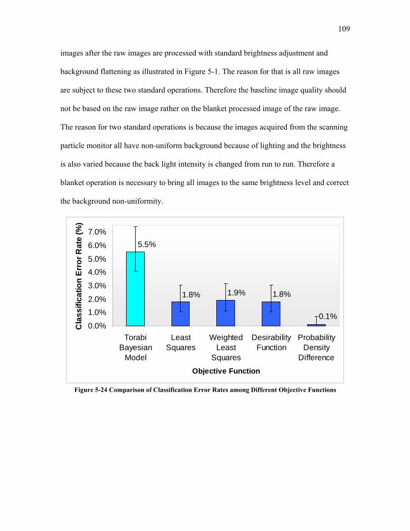
109
images after the raw images are processed with standard brightness adjustment and
background flattening as illustrated in Figure 5-1. The reason for that is all raw images
are subject to these two standard operations. Therefore the baseline image quality should
not be based on the raw image rather on the blanket processed image of the raw image.
The reason for two standard operations is because the images acquired from the scanning
particle monitor all have non-uniform background because of lighting and the brightness
is also varied because the back light intensity is changed from run to run. Therefore a
blanket operation is necessary to bring all images to the same brightness level and correct
the background non-uniformity.
0.1%
5.5%
1.8% 1.9% 1.8%
0.0%
1.0%2.0%
3.0%
4.0%5.0%
6.0%
7.0%
TorabiBayesian
Model
LeastSquares
WeightedLeast
Squares
DesirabilityFunction
ProbabilityDensity
DifferenceObjective Function
Cla
ssifi
catio
n Er
ror R
ate
(%)
Figure 5-24 Comparison of Classification Error Rates among Different Objective Functions
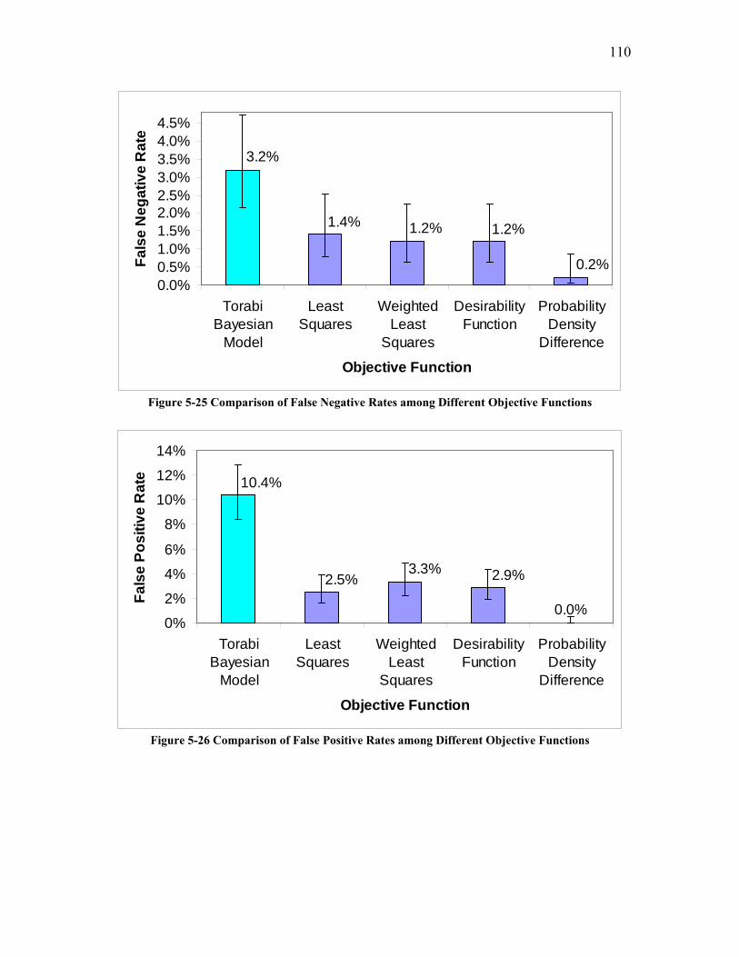
110
3.2%
1.4% 1.2% 1.2%
0.2%0.0%0.5%1.0%1.5%2.0%2.5%3.0%3.5%4.0%4.5%
TorabiBayesian
Model
LeastSquares
WeightedLeast
Squares
DesirabilityFunction
ProbabilityDensity
Difference
Objective Function
Fals
e N
egat
ive
Rat
e
Figure 5-25 Comparison of False Negative Rates among Different Objective Functions
0.0%
2.9%3.3%2.5%
10.4%
0%
2%
4%
6%
8%
10%
12%
14%
TorabiBayesian
Model
LeastSquares
WeightedLeast
Squares
DesirabilityFunction
ProbabilityDensity
Difference
Objective Function
Fals
e Po
sitiv
e R
ate
Figure 5-26 Comparison of False Positive Rates among Different Objective Functions

111
0
0.1
0.2
0.3
0.4
0.5
0.6
0.7
0.8
0.9
1
0 0.2 0.4 0.6 0.8 1False Positive Rate
True
Pos
itive
Rat
e
Raw Images Least SquaresWeighted Least Squares Desirability FunctionProbability Density Difference
Figure 5-27 ROC Analysis of the Classification Performance of Different Objective Functions
Table 5-15 Comparison of AUC among Different Objective Functions
Objection Function (Area Under the
ROC curve) AUC
No Objective Function (Torabi Bayesian Model of Raw Images)
0.974
Least Squares 0.998 Weighted Least Squares 0.991 Desirability Function 0.996 Probability Density Difference 1
Table 5-16 Image Quality Metrics for the Training Image Set After Blanket Processing
Brightness Contrast Blur Noise Illumination uniformity
Local contrast
Average 0.42 0.075 0.47 0.69 0.89 0.49 95% Confidence
Interval on Average ±0.0004 ±0.004 ±0.01 ±0.01 ±0.014 ±0.02
Minimum 0.39 0.019 0 0.38 0.18 0.03 Maximum 0.43 0.43 1 0.94 1 1

112
Table 5-16 shows the average, confidence interval, minimum and maximum for each
individual five image quality metric. It should be noted that the values of these IQ
Metrics are between 0 and unity. In general, the training set images have a rather low
contrast with an average of 0.075. Most images are blurry with an average blurriness of
0.47 and range from 0 to 1, meaning from the worst to the best. The training images’
noise level is moderate with an average of 0.69 but it varies from 0.38 to 0.94. The
training images have high illumination uniformity but again the range of it is from 0.18 to
1. The average local contrast of potential particles is moderate with an average of 0.49.
The table shows that the training image set contains a variety of image. During the off-
line image modification, the selection of image operators are based on the image quality
metrics of an individual image not the average values list in the table.
In the next section the data obtained from off-line image modification is used to provide
the basis for a method of in-line image modification to improve classification of
“unknown” images. Images from new extrusion monitoring experiments are added to
images previously provided by Torabi and a method for adapting the in-line image
processing to large change in the quality of a raw image is developed.
The average image quality optimization time per image was 176 seconds, using a
Pentium 4 Windows NT station.
113
5.2 In-line Image Quality Modification This section of the thesis shows how the second objective was accomplished. That is, it
shows the development of an in-line method for modifying image quality to improve
classification. As outlined in Section 2.4.1, the strategy is to utilize the results of the first
objective to formulate the needed “Reference Image Database”. Subsequent steps in the
strategy involve using this database to provide the means for correctly modifying new
“unknown” images and finally adding adaptability to the system with experimental
verification to demonstrate its utility. In the next section the Reference Image Database
is described. It is the link between the off-line image modification classification results
reported in Section 5.1 and the new classification results to be reported in this section
obtained by in-line classifying “unknown” images. Following that, this section shows
how this database is used with a static (not adaptive) classification models to obtain the
in-line classification results. Finally, in Section 5.2.3 the results of making the model
adaptive are shown.
5.2.1 The Reference Image Database The whole purpose of the first objective was to determine how best to modify a variety of
images so that their classification as WO or WP would be improved. “Known” images
were used (i.e. as the software was informed of the actual class, WO or WP). Another
way of stating this is to say that accomplishing Objective 1 provides the Reference Image
Database. In-line image quality improvement will be done by (a) locating the image in
this database that most closely resembles a newly received “unknown” image and (b)
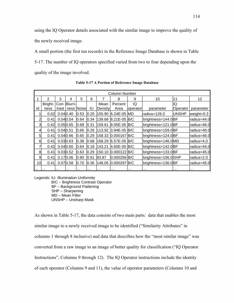
114
using the IQ Operator details associated with the similar image to improve the quality of
the newly received image.
A small portion (the first ten records) in the Reference Image Database is shown in Table
5-17. The number of IQ operators specified varied from two to four depending upon the
quality of the image involved.
Table 5-17 A Portion of Reference Image Database
Column Number 1 2 3 4 5 6 7 8 9 10 11 12
id Bright-ness
Con- trast
Blurri- ness Noise IU
MeanDensity
PercentArea
IQ operator parameter
IQ Operator parameter
1 0.62 0.04 0.40 0.53 0.25 155.90 6.24E-05 MD radius=126.0 UNSHP weight=0.32 0.41 0.04 0.54 0.64 0.34 139.68 8.21E-05 B/C brightness=144.0 BF radius=44.03 0.42 0.05 0.65 0.68 0.31 159.61 8.05E-05 B/C brightness=121.0 BF radius=46.04 0.41 0.04 0.51 0.66 0.26 113.92 3.94E-05 B/C brightness=159.0 BF radius=40.05 0.41 0.04 0.66 0.65 0.29 158.33 0.000167 B/C brightness=124.0 BF radius=46.06 0.41 0.03 0.63 0.38 0.68 168.29 6.57E-05 B/C brightness=146.0 MD radius=4.07 0.42 0.04 0.60 0.64 0.18 143.21 4.60E-05 B/C brightness=142.0 BF radius=44.08 0.41 0.03 0.52 0.63 0.29 150.10 0.000122 B/C brightness=133.0 BF radius=45.09 0.41 0.17 0.06 0.90 0.91 83.87 0.000256 B/C brightness=106.0 SHP radius=2.0
10 0.41 0.07 0.58 0.70 0.36 148.05 0.000297 B/C brightness=136.0 BF radius=45.0… … … … … … … … … … … … Legends: IU- Illumination Uniformity B/C – Brightness Contrast Operator BF – Background Flattening SHP – Sharpening MD – Mean Filter UNSHP – Unsharp Mask As shown in Table 5-17, the data consists of two main parts: data that enables the most
similar image to a newly received image to be identified (“Similarity Attributes” in
columns 1 through 8 inclusive) and data that describes how the “most similar image” was
converted from a raw image to an image of better quality for classification (“IQ Operator
Instructions”, Columns 9 through 12). The IQ Operator instructions include the identity
of each operator (Columns 9 and 11), the value of operator parameters (Columns 10 and

115
12) and the order of application of the operators (same as the order presented in the table
read from left to right). Considering record 6 in Table 12 for example, the “IQ Operators
instructions” are operator brightness/contrast shift (“B/C” for short) with parameter
brightness set at 146.0 followed by another operator media filter with parameter radius
set at 4.0.
The similarity attributes include the five image quality metrics (mostly statistical image
features): brightness, contrast, blur, noise and illumination uniformity. In addition, the
similarity attributes include the two attributes that are actually used in the Torabi
classification model in this work: percentage area and mean density of potential
particles. As shown by Torabi [2], as well as by preliminary testing of his model for this
work, the other attributes were ineffective because they were highly inter-correlated.
The database is organized in a flat structure; that is, one case following by another case
without ordering. However, it does have two blocks: one block of cases is for images
with high local contrast and the other for images with low local contrast. This aspect will
be described more fully in Section 5.2.3.5. Within each block, the records are placed
randomly.
The Reference Image Database can grow to accommodate new image cases when these
new image cases are initially misclassified in in-line image modification. The
misclassified images are subjected to customized, off-line image modification and the
results were added to the Reference Image Database. For the static classification model
predictions (reported in the next section) the database contained 745 records.

116
5.2.2 In-line Image Quality Modification for Classification: Use of a Static Classification Model
A classification model is termed “static” when it is not updated with new cases. This
section will report on the results of using static pre-optimization and static post-
optimization classification models.
Earlier, Figure 5-1 described how a training image was processed to provide the
information necessary to compose the Reference Image Database and create pre-
optimization and post-optimization classification models. Figure 5-28 shows how the
Reference Image Database along with the pre-optimization and post-optimization
classification models is used to modify and classify “unknown” test images (a test image
is not used to compose the Reference Image Database and its information is not used to
create pre-optimization and post-optimization models in cross-validation. Since the test
image is an “unknown” image it means that the software is unaware of the actual class of
the image but we are.) in-line based on the strategy presented in Section 2.4. This
method is termed the “Image Quality Modification for Classification” model (termed
IQMod Classification”). As shown in Figure 5-28, we see that the test raw image first is
processed with two baseline operations: brightness adjustment and background flattening.
The processed image is then measured for the seven similarity attributes mentioned in
Table 5-18. Next, case-based reasoning is used to find the most similar case in the
Reference Image Database. The most similar case is the one in the Reference Image
Database with the shortest Euclidean distance to the new image. The Euclidean distance

117
is calculated from Equation 5-6. Specifying the actual similarity attributes used this
equation becomes:
∑=
−=7
1
2, )(
iiDBi SSD 5-6
where Si is the value of the ith similarity attribute for the new image and SDB,i is the
corresponding value for an image in the Reference Image Database. The similarity
attribute corresponding to each value of i is shown in Table 5-18.
Table 5-18 Similarity Attributes
i Similarity Attribute 1 Brightness 2 Contrast 3 Blur 4 Noise 5 Illumination Uniformity 6 Mean Density 7 Percentage Area
The image operators and their parameters associated with the image in the Reference
Image Database giving the lowest value of D from Equation 5-6 is then applied to
process the new image. The processed new image is then classified using the post-
optimization model classification model developed using training image set in off-line
image quality modification (as shown in Figure 5-1) . Static classification models
(including both the pre-optimization model and the post-optimization model) were earlier
created in the off-line image modification (see the created models in Section 5.1.2.4)
using the set of training images (in Table 5-2) being repeatedly used for the four image
quality definition throughout the off-line image modification. The set of training images
are from 8 experimental extrusion runs carried out in previous research by Torabi.

118
Using these models described in the Section 5.1 (as shown in Table 5-13), a set of 2888
“unknown” test images (a subset of Image Set 1 in Table 3-1 from Torabi’s research) is
used to test the performance of IQMod Classification. The classification results are
provided in Table 5-19.
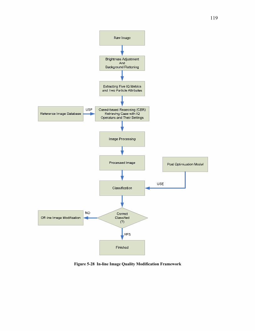
119
Figure 5-28 In-line Image Quality Modification Framework
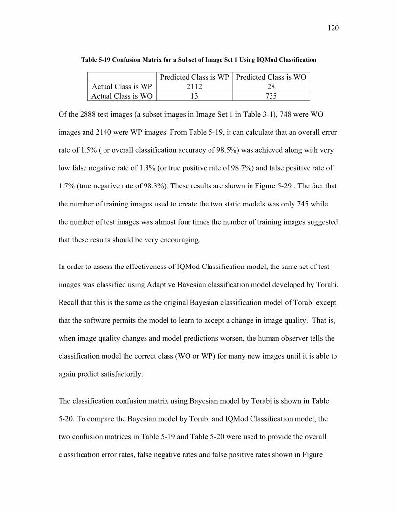
120
Table 5-19 Confusion Matrix for a Subset of Image Set 1 Using IQMod Classification
Predicted Class is WP Predicted Class is WO
Actual Class is WP 2112 28 Actual Class is WO 13 735
Of the 2888 test images (a subset images in Image Set 1 in Table 3-1), 748 were WO
images and 2140 were WP images. From Table 5-19, it can calculate that an overall error
rate of 1.5% ( or overall classification accuracy of 98.5%) was achieved along with very
low false negative rate of 1.3% (or true positive rate of 98.7%) and false positive rate of
1.7% (true negative rate of 98.3%). These results are shown in Figure 5-29 . The fact that
the number of training images used to create the two static models was only 745 while
the number of test images was almost four times the number of training images suggested
that these results should be very encouraging.
In order to assess the effectiveness of IQMod Classification model, the same set of test
images was classified using Adaptive Bayesian classification model developed by Torabi.
Recall that this is the same as the original Bayesian classification model of Torabi except
that the software permits the model to learn to accept a change in image quality. That is,
when image quality changes and model predictions worsen, the human observer tells the
classification model the correct class (WO or WP) for many new images until it is able to
again predict satisfactorily.
The classification confusion matrix using Bayesian model by Torabi is shown in Table
5-20. To compare the Bayesian model by Torabi and IQMod Classification model, the
two confusion matrices in Table 5-19 and Table 5-20 were used to provide the overall
classification error rates, false negative rates and false positive rates shown in Figure
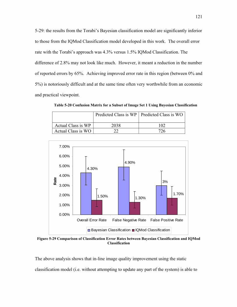
121
5-29: the results from the Torabi’s Bayesian classification model are significantly inferior
to those from the IQMod Classification model developed in this work. The overall error
rate with the Torabi’s approach was 4.3% versus 1.5% IQMod Classification. The
difference of 2.8% may not look like much. However, it meant a reduction in the number
of reported errors by 65%. Achieving improved error rate in this region (between 0% and
5%) is notoriously difficult and at the same time often very worthwhile from an economic
and practical viewpoint.
Table 5-20 Confusion Matrix for a Subset of Image Set 1 Using Bayesian Classification
Predicted Class is WP Predicted Class is WO
Actual Class is WP 2038 102 Actual Class is WO 22 726
3%
4.30%4.90%
1.70%1.30%1.50%
0.00%
1.00%
2.00%
3.00%
4.00%
5.00%
6.00%
7.00%
Overall Error Rate False Negative Rate False Positive Rate
Rat
e
Bayesian Classification IQMod Classification
Figure 5-29 Comparison of Classification Error Rates between Bayesian Classification and IQMod Classification
The above analysis shows that in-line image quality improvement using the static
classification model (i.e. without attempting to update any part of the system) is able to

122
decrease classification error rate very effectively. To see if further improvement could be
obtained and to show how the developed method could be adapted to a different image
quality, an extensive body of other images was obtained and In-line Adaptive Image
Quality Modification with Adaptive Classification model (Adaptive IQMod
Classification) was developed. The development and extensive testing of this
comprehensive model is described in the next section.
5.2.3 In-line Adaptive Image Quality Modification with Adaptive Classification
At this point the work is concerned with the following four models:
In-line Bayesian Classification is the conventional Naïve Bayesian model originally
applied by Torabi to classify images as WO or WP. It accepts as input the percentage
area and the average particle image density of an image.
In-line Adaptive Bayesian Classification is the same as the Bayesian classification
model except that, as mentioned in the previous section, the software permits the
model to learn to accept a change in image quality. That is, when image quality
changes and model predictions worsen, the human observer teaches the software
using many new images to enable it once again to predict satisfactorily.
In-line Image Quality Modification for Bayesian Classification (“IQMod
Classification”) is the use of the Reference Image Database and Case Based
Reasoning along with the pre-optimization Bayesian classification model to
determine how best to modify a new image to improve classification. It also includes
the use of a post-optimization Bayesian classification model to classify new
123
“Unknown” images as WO or WP. Figure 5-28 summarizes this approach and it was
explained in detail in Section 5.2.2. The assessment of the previous section showed
that this approach provided superior results to the In-line Adaptive Bayesian
classification model for the same test images used by Torabi.
In-line Adaptive Image Quality Modification for Adaptive Bayesian
Classification (termed “Adaptive IQMod Classification”) the fourth model is the
subject of this section of the thesis.
This model adapts IQMod Classification to changes in image quality and combines it
with the Adaptive Bayesian model. This required adapting three parts of the system: the
Reference Image Database and each of the two Bayesian classification models (the pre-
optimization and post-optimization classification models). The actual adaptation was
done by using misclassified images as they were obtained. That is, if an image was
misclassified, then this image was subject to the process of off-line image quality
improvement as illustrated in Figure 5-1. The off-line image quality improvement added
relevant information related to the image including IQ metrics of the image and IQ
operator instructions for the image to the Reference Image Database after image quality
optimization. At the same time, this image was used to update the pre-optimization model
and its optimized image was used to update the post-optimization model. Accordingly,
the adaptability of this model resulted from two actions: a) incrementing the Reference
Image Database with IQ operator instructions acquired from customized optimization of
the misclassified image; b) adapting the pre-optimization and post-optimization
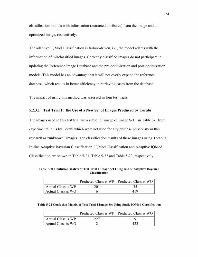
124
classification models with information (extracted attributes) from the image and its
optimized image, respectively.
The adaptive IQMod Classification is failure-driven, i.e., the model adapts with the
information of misclassified images. Correctly classified images do not participate in
updating the Reference Image Database and the pre-optimization and post-optimization
models. This model has an advantage that it will not overly expand the reference
database, which results in better efficiency in retrieving cases from the database.
The impact of using this method was assessed in four test trials:
5.2.3.1 Test Trial 1: the Use of a New Set of Images Produced by Torabi The images used in this test trial are a subset of image of Image Set 1 in Table 3-1 from
experimental runs by Torabi which were not used for any purpose previously in this
research as “unknown” images. The classification results of these images using Torabi’s
In-line Adaptive Bayesian Classification, IQMod Classification and Adaptive IQMod
Classification are shown in Table 5-21, Table 5-22 and Table 5-23, respectively.
Table 5-21 Confusion Matrix of Test Trial 1 Image Set Using In-line Adaptive Bayesian
Classification
Predicted Class is WP Predicted Class is WO Actual Class is WP 201 35 Actual Class is WO 6 419
Table 5-22 Confusion Matrix of Test Trial 1 Image Set Using Static IQMod Classification
Predicted Class is WP Predicted Class is WO Actual Class is WP 227 9 Actual Class is WO 2 423

125
Table 5-23 Confusion Matrix of Test Trial 1 Image Set Using Adaptive IQMod Classification
Predicted Class is WP Predicted Class is WO
Actual Class is WP 235 1 Actual Class is WO 3 422
As shown in Figure 5-30, the overall classification error rate of Adaptive IQMod
Classification was 0.6%. This is 8.8% and 1.1% less than that of the Adaptive Bayesian
Classification and IQMod Classification.
The analysis above demonstrates that the classification error rate was significantly
reduced for Adaptive IQMod Classification over the other two models. It shows that the
combination of a “failure-driven”, incremental, case-based reasoning method and
Bayesian adaptive classification models is very powerful in terms of dealing with image
quality variability.
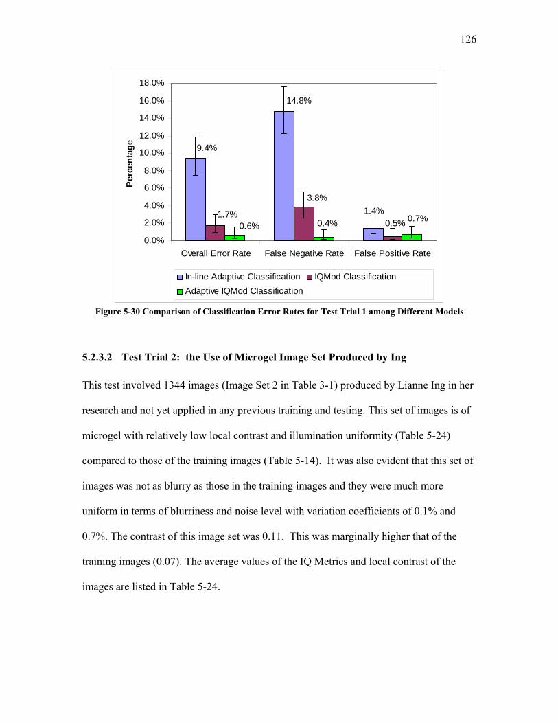
126
1.4%
14.8%
9.4%
0.5%
3.8%
1.7%0.4% 0.7%
0.6%0.0%
2.0%
4.0%
6.0%
8.0%
10.0%
12.0%
14.0%
16.0%
18.0%
Overall Error Rate False Negative Rate False Positive Rate
Per
cent
age
In-line Adaptive Classification IQMod ClassificationAdaptive IQMod Classification
Figure 5-30 Comparison of Classification Error Rates for Test Trial 1 among Different Models
5.2.3.2 Test Trial 2: the Use of Microgel Image Set Produced by Ing This test involved 1344 images (Image Set 2 in Table 3-1) produced by Lianne Ing in her
research and not yet applied in any previous training and testing. This set of images is of
microgel with relatively low local contrast and illumination uniformity (Table 5-24)
compared to those of the training images (Table 5-14). It was also evident that this set of
images was not as blurry as those in the training images and they were much more
uniform in terms of blurriness and noise level with variation coefficients of 0.1% and
0.7%. The contrast of this image set was 0.11. This was marginally higher that of the
training images (0.07). The average values of the IQ Metrics and local contrast of the
images are listed in Table 5-24.
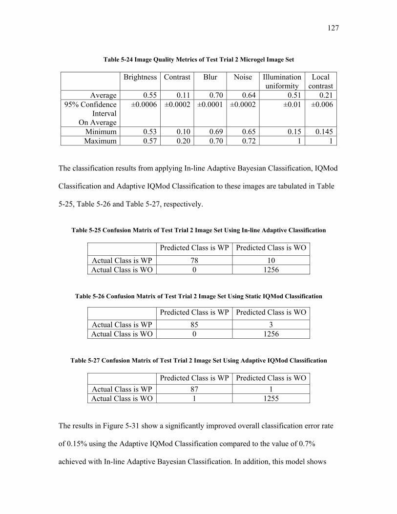
127
Table 5-24 Image Quality Metrics of Test Trial 2 Microgel Image Set
Brightness Contrast Blur Noise Illumination
uniformity Local
contrastAverage 0.55 0.11 0.70 0.64 0.51 0.21
95% Confidence Interval
On Average
±0.0006 ±0.0002 ±0.0001 ±0.0002 ±0.01 ±0.006
Minimum 0.53 0.10 0.69 0.65 0.15 0.145Maximum 0.57 0.20 0.70 0.72 1 1
The classification results from applying In-line Adaptive Bayesian Classification, IQMod
Classification and Adaptive IQMod Classification to these images are tabulated in Table
5-25, Table 5-26 and Table 5-27, respectively.
Table 5-25 Confusion Matrix of Test Trial 2 Image Set Using In-line Adaptive Classification
Predicted Class is WP Predicted Class is WO
Actual Class is WP 78 10 Actual Class is WO 0 1256
Table 5-26 Confusion Matrix of Test Trial 2 Image Set Using Static IQMod Classification
Predicted Class is WP Predicted Class is WO Actual Class is WP 85 3 Actual Class is WO 0 1256
Table 5-27 Confusion Matrix of Test Trial 2 Image Set Using Adaptive IQMod Classification
Predicted Class is WP Predicted Class is WO Actual Class is WP 87 1 Actual Class is WO 1 1255
The results in Figure 5-31 show a significantly improved overall classification error rate
of 0.15% using the Adaptive IQMod Classification compared to the value of 0.7%
achieved with In-line Adaptive Bayesian Classification. In addition, this model shows
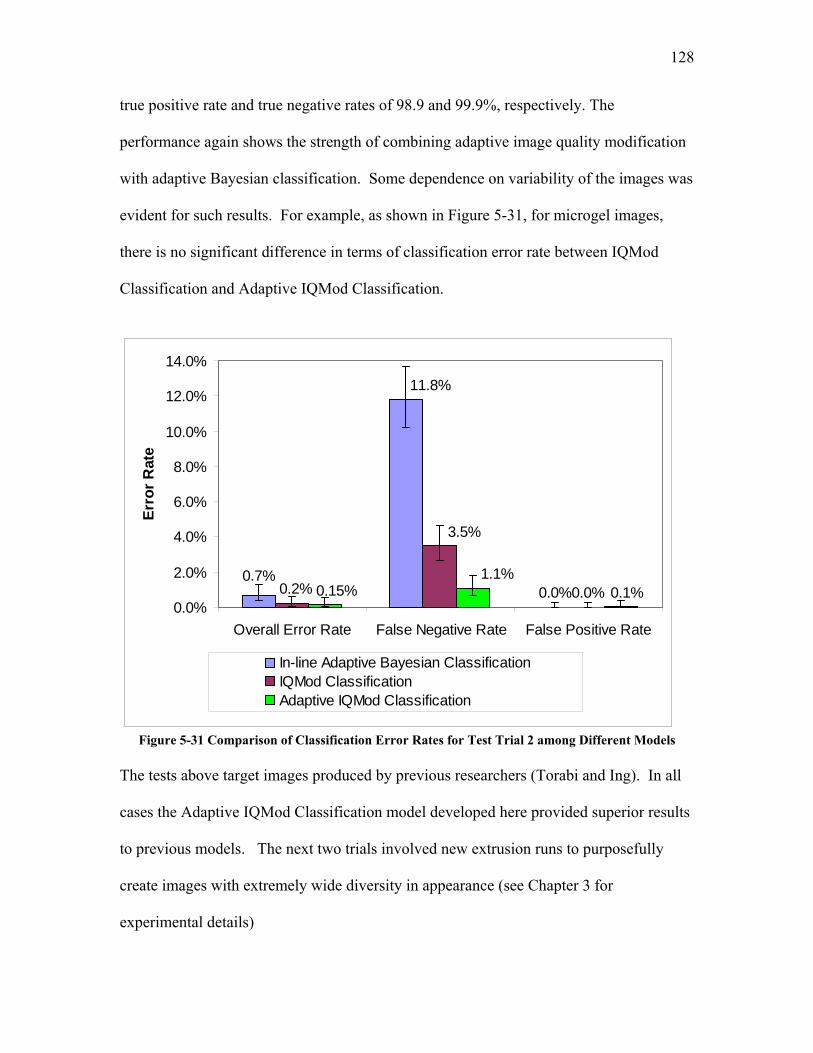
128
true positive rate and true negative rates of 98.9 and 99.9%, respectively. The
performance again shows the strength of combining adaptive image quality modification
with adaptive Bayesian classification. Some dependence on variability of the images was
evident for such results. For example, as shown in Figure 5-31, for microgel images,
there is no significant difference in terms of classification error rate between IQMod
Classification and Adaptive IQMod Classification.
0.0%0.0%
11.8%
0.7%
3.5%
0.2% 0.15%1.1%
0.1%0.0%
2.0%
4.0%
6.0%
8.0%
10.0%
12.0%
14.0%
Overall Error Rate False Negative Rate False Positive Rate
Erro
r Rat
e
In-line Adaptive Bayesian ClassificationIQMod ClassificationAdaptive IQMod Classification
Figure 5-31 Comparison of Classification Error Rates for Test Trial 2 among Different Models
The tests above target images produced by previous researchers (Torabi and Ing). In all
cases the Adaptive IQMod Classification model developed here provided superior results
to previous models. The next two trials involved new extrusion runs to purposefully
create images with extremely wide diversity in appearance (see Chapter 3 for
experimental details)

129
5.2.3.3 Test Trial 3: the Use of Images from New Extruder Runs Utilizing Injection of Particles with Low Additive Polyethylene Pelletized Feed
In general, the images generated from 530A polyethylene pellets (a subset of 1472
images of Image Set 3 as from run 3-1 to run 3-4 in Table 3-2) had consistently lower
values of average image quality metrics (Table 5-28) than those of the training images
(Table 5-14).
Table 5-28 Image Quality Metrics of Test Trial 3 Image Set
Brightness Contrast Blur Noise Illumination
uniformity Local
contrast Average 0.40 0.034 0.37 0.57 0.71 0.24
95% Confidence Interval
On Average
±0.0003 ±0.001 ±0.039 ±0.007 ±0.025 ±0.007
Minimum 0.39 0.019 0 0.47 0.27 0.094 Maximum 0.41 0.067 1 0.77 1 0.48
The classification confusion matrices for this set of images are tabulated in Table 5-29 ~
33 and the classification error rates are illustrated in Figure 5-32. From these tables and
figure, we see that the highest overall classification error rate is 1.5% for pure 530A
polyethylene pellets. Even when no particles were added, particles were present in
extrusion of pure 530A because of residuals remaining from previous extrusion runs
where particles were intentionally added. For images when 200ppm 30µm GMS is added,
the classification accuracy reaches 100%, meaning an error rate of zero. For images
captured with the addition of 40ppm 100µm-GMS to the 530A polymer, the overall error
rate is 0.1% (or accuracy of 99.9%) with a false positive rate of 0%. The classification
error rate for images with the addition of 20ppm glass bubbles to feed is 1.2% with a
“balanced” false negative rate of 0.8% and false positive rate of 2.0% (or true negative
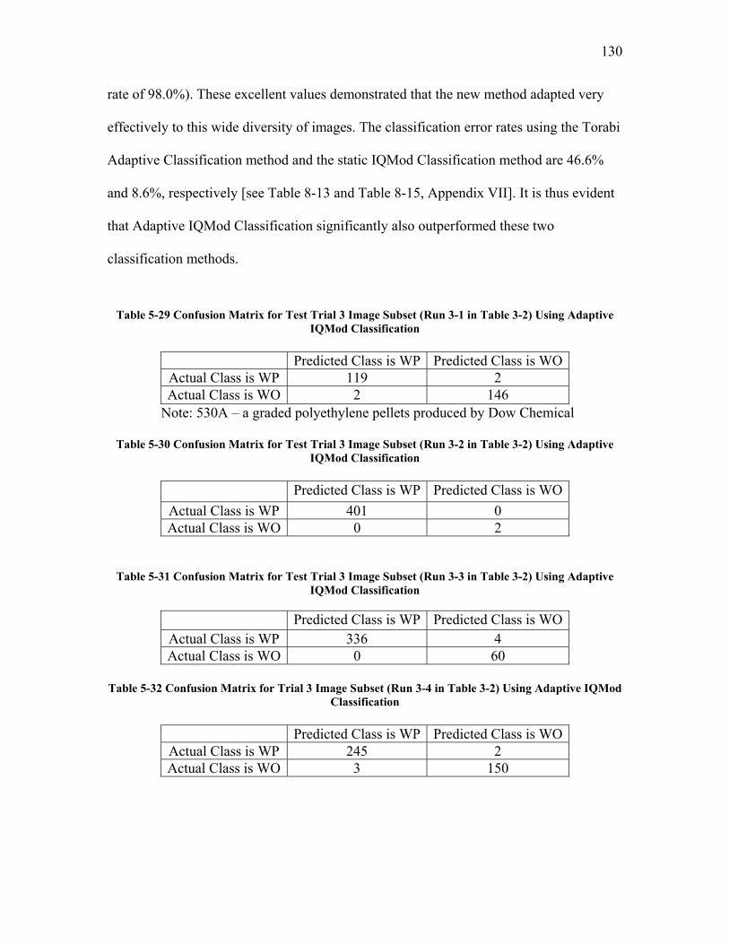
130
rate of 98.0%). These excellent values demonstrated that the new method adapted very
effectively to this wide diversity of images. The classification error rates using the Torabi
Adaptive Classification method and the static IQMod Classification method are 46.6%
and 8.6%, respectively [see Table 8-13 and Table 8-15, Appendix VII]. It is thus evident
that Adaptive IQMod Classification significantly also outperformed these two
classification methods.
Table 5-29 Confusion Matrix for Test Trial 3 Image Subset (Run 3-1 in Table 3-2) Using Adaptive
IQMod Classification
Predicted Class is WP Predicted Class is WO Actual Class is WP 119 2 Actual Class is WO 2 146
Note: 530A – a graded polyethylene pellets produced by Dow Chemical
Table 5-30 Confusion Matrix for Test Trial 3 Image Subset (Run 3-2 in Table 3-2) Using Adaptive IQMod Classification
Predicted Class is WP Predicted Class is WO
Actual Class is WP 401 0 Actual Class is WO 0 2
Table 5-31 Confusion Matrix for Test Trial 3 Image Subset (Run 3-3 in Table 3-2) Using Adaptive IQMod Classification
Predicted Class is WP Predicted Class is WO
Actual Class is WP 336 4 Actual Class is WO 0 60
Table 5-32 Confusion Matrix for Trial 3 Image Subset (Run 3-4 in Table 3-2) Using Adaptive IQMod
Classification
Predicted Class is WP Predicted Class is WO Actual Class is WP 245 2 Actual Class is WO 3 150

131
1.2%1.0%
1.5%
0.0% 0.0%
1.2%
1.6% 0.8%2.0%
0.0% 0.0%
1.3%
0.0%
0.5%
1.0%
1.5%
2.0%
2.5%
3.0%
3.5%
4.0%
4.5%
530A 530A + 30µmGMS – 200ppm
530A + 100µmGMS – 40ppm
530A + Glass bubbles -20ppm
Erro
r Rat
e
Overall Error Rate False Negative Rate False Positive Rate
Figure 5-32 Classification Error Rates for Test Trial 3 Using Adaptive IQMod Classification
5.2.3.4 Test Trial 4: the Use of Images from New Extrusion Runs Utilizing Injection of Particles with High Additive Polyethylene Pelletized Feed
These images (a subset of 538 images of Image Set 3 in Table 3-1 and the same set of
images as in Run 3-5 and 3-6 in Table 3-2, and hereinafter called Batch-A) initially
proved the most difficult of all. The classification results are shown in Table 5-33, Table
5-34 and displayed in Figure 5-33 . The result shows that the classification error rates for
Batch-A without the addition of particles and Batch-A with the addition of 75µm glass
beads are 17.1% and 29.7%. False positive rate for images from Batch-A with the
addition of 75µm glass beads was also disappointing at 56.6% though a reasonably false
negative rate of 8.2% (or a true positive rate of 91.8%) was obtained.
This result above exposed a weakness that the system has not previously encountered. To
define this weakness, an analysis of image quality was carried out. Table 5-35 shows the
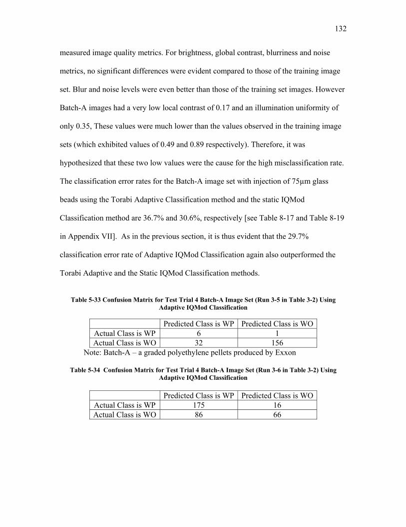
132
measured image quality metrics. For brightness, global contrast, blurriness and noise
metrics, no significant differences were evident compared to those of the training image
set. Blur and noise levels were even better than those of the training set images. However
Batch-A images had a very low local contrast of 0.17 and an illumination uniformity of
only 0.35, These values were much lower than the values observed in the training image
sets (which exhibited values of 0.49 and 0.89 respectively). Therefore, it was
hypothesized that these two low values were the cause for the high misclassification rate.
The classification error rates for the Batch-A image set with injection of 75µm glass
beads using the Torabi Adaptive Classification method and the static IQMod
Classification method are 36.7% and 30.6%, respectively [see Table 8-17 and Table 8-19
in Appendix VII]. As in the previous section, it is thus evident that the 29.7%
classification error rate of Adaptive IQMod Classification again also outperformed the
Torabi Adaptive and the Static IQMod Classification methods.
Table 5-33 Confusion Matrix for Test Trial 4 Batch-A Image Set (Run 3-5 in Table 3-2) Using
Adaptive IQMod Classification
Predicted Class is WP Predicted Class is WO Actual Class is WP 6 1 Actual Class is WO 32 156
Note: Batch-A – a graded polyethylene pellets produced by Exxon
Table 5-34 Confusion Matrix for Test Trial 4 Batch-A Image Set (Run 3-6 in Table 3-2) Using Adaptive IQMod Classification
Predicted Class is WP Predicted Class is WO
Actual Class is WP 175 16 Actual Class is WO 86 66
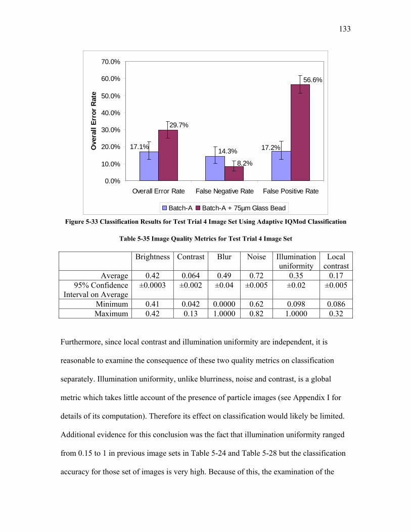
133
17.2%17.1% 14.3%
56.6%
29.7%
8.2%
0.0%
10.0%
20.0%
30.0%
40.0%
50.0%
60.0%
70.0%
Overall Error Rate False Negative Rate False Positive Rate
Ove
rall
Erro
r R
ate
Batch-A Batch-A + 75µm Glass Bead
Figure 5-33 Classification Results for Test Trial 4 Image Set Using Adaptive IQMod Classification
Table 5-35 Image Quality Metrics for Test Trial 4 Image Set
Brightness Contrast Blur Noise Illumination uniformity
Local contrast
Average 0.42 0.064 0.49 0.72 0.35 0.17 95% Confidence
Interval on Average ±0.0003 ±0.002 ±0.04 ±0.005 ±0.02 ±0.005
Minimum 0.41 0.042 0.0000 0.62 0.098 0.086 Maximum 0.42 0.13 1.0000 0.82 1.0000 0.32
Furthermore, since local contrast and illumination uniformity are independent, it is
reasonable to examine the consequence of these two quality metrics on classification
separately. Illumination uniformity, unlike blurriness, noise and contrast, is a global
metric which takes little account of the presence of particle images (see Appendix I for
details of its computation). Therefore its effect on classification would likely be limited.
Additional evidence for this conclusion was the fact that illumination uniformity ranged
from 0.15 to 1 in previous image sets in Table 5-24 and Table 5-28 but the classification
accuracy for those set of images is very high. Because of this, the examination of the

134
failure was centered on local contrast. Local contrast measures the contrast of potential
particles against their immediate background.
5.2.3.5 The Application of Decision Rule in Case-based Reasoning (CBR) Examining the misclassified cases in the Batch-A image (in Table 5-34) showed that the
case-based reasoning retrieved most similar image cases in the Reference Image
Database having a much higher local contrast (defined below in Equation 5-7) than those
of their corresponding misclassified Batch-A images. Therefore a large number of
misclassified images with low local contrast were processed with IQ operator instructions
suited to higher local contrast images. This led to the misclassification. It also meant that
the Euclidean distance function used to retrieve the image case similar to the current
image failed in this situation.
Local contrast is defined by:
B
PB
GGG
ContrastLocal−
= 5-7
where GP is the mean density (mean grey level) of all particles present, and GB is the
mean grey level of the immediate background of the particles.
Recall that local contrast is not one of the similarity attributes (in Table 5-18 ) used in
Euclidean distance function for similarity measurement between two images. Instead
global contrast (defined below in Equation 5-8) is used. Global contrast is defined by:
MinMax
MinMax
LLLL
ContrastGlobal+−
= 5-8

135
where Lmax and Lmin is the maximum grey level and minimum grey level of an entire
image (both particles and background considered together).
It was hypothesized that the existing Euclidean distance measure would still be suitable if
it could be applied to images with similar local contrast values. Splitting the database
into low and high local contrast image blocks is the simplest approach and could work
depending on the nature of the variability of local contrast in the images and the tolerance
for variability in local contrast of the case-based reasoning approach using the Euclidean
distance measure. The approach used was to specify a threshold local contrast value and
divide the Reference Image Database into two parts above and below that value. Figure
5-34 shows a flow chart illustrating the method.
Figure 5-34 The Application of Decision Rule in Case-Based Reasoning

136
For each image, after the usual blanket operations, the local contrast and other IQ Metrics
were measured. If the local contrast of an image was higher than the threshold value,
Case Based Reasoning would find the most similar image case in the high local contrast
block in the Reference Image Database; otherwise, the case retrieval was executed in the
low local contrast block. This process only affected which block of images was selected
to be the Reference Image Database for a particular image. The remainder of the method
was the same as specified in Figure 5-28.
5.2.3.6 Classification Results after the Application of Decision Rule in Case-Based Reasoning
To implement the method of dividing the Reference Image Database into two parts it was
necessary to determine the best threshold value of local contrast. This was done by trial
and error.
The effect of the threshold of local contrast on classification error rate for Batch-A
images (shown in Table 5-34) is listed in Table 5-36. For each threshold dividing the
reference database, classification on the Batch-A images was performed and the
classification accuracy was recorded. The result shows a general trend: as the threshold of
local contrast increased, the true positive rate decreased while false positive rate
increased. However, the overall classification accuracy increased, reached a peak and
then decreased. The classification error rate reached the lowest value (5.25%) at a
threshold of local contrast of 0.171. At that point the false negative rate and the false
positive rate also reached their lowest values (5.24% and 5.26% respectively).
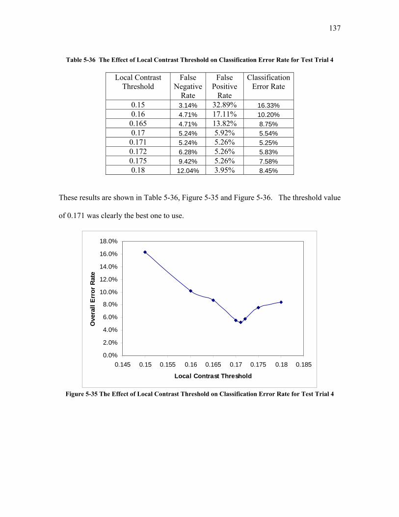
137
Table 5-36 The Effect of Local Contrast Threshold on Classification Error Rate for Test Trial 4
Local Contrast
Threshold False
Negative Rate
False Positive
Rate
Classification Error Rate
0.15 3.14% 32.89% 16.33% 0.16 4.71% 17.11% 10.20% 0.165 4.71% 13.82% 8.75% 0.17 5.24% 5.92% 5.54% 0.171 5.24% 5.26% 5.25% 0.172 6.28% 5.26% 5.83% 0.175 9.42% 5.26% 7.58% 0.18 12.04% 3.95% 8.45%
These results are shown in Table 5-36, Figure 5-35 and Figure 5-36. The threshold value
of 0.171 was clearly the best one to use.
0.0%
2.0%
4.0%
6.0%
8.0%
10.0%
12.0%
14.0%
16.0%
18.0%
0.145 0.15 0.155 0.16 0.165 0.17 0.175 0.18 0.185
Local Contrast Threshold
Ove
rall
Err
or R
ate
Figure 5-35 The Effect of Local Contrast Threshold on Classification Error Rate for Test Trial 4
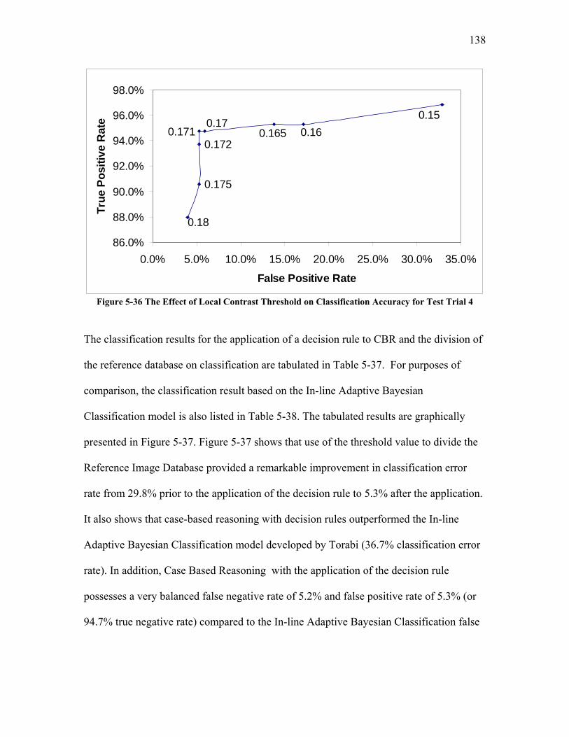
138
0.170.171
0.150.160.165
0.172
0.175
0.18
86.0%
88.0%
90.0%
92.0%
94.0%
96.0%
98.0%
0.0% 5.0% 10.0% 15.0% 20.0% 25.0% 30.0% 35.0%
False Positive Rate
True
Pos
itive
Rat
e
Figure 5-36 The Effect of Local Contrast Threshold on Classification Accuracy for Test Trial 4
The classification results for the application of a decision rule to CBR and the division of
the reference database on classification are tabulated in Table 5-37. For purposes of
comparison, the classification result based on the In-line Adaptive Bayesian
Classification model is also listed in Table 5-38. The tabulated results are graphically
presented in Figure 5-37. Figure 5-37 shows that use of the threshold value to divide the
Reference Image Database provided a remarkable improvement in classification error
rate from 29.8% prior to the application of the decision rule to 5.3% after the application.
It also shows that case-based reasoning with decision rules outperformed the In-line
Adaptive Bayesian Classification model developed by Torabi (36.7% classification error
rate). In addition, Case Based Reasoning with the application of the decision rule
possesses a very balanced false negative rate of 5.2% and false positive rate of 5.3% (or
94.7% true negative rate) compared to the In-line Adaptive Bayesian Classification false

139
negative rate of 61.3% and false positive rate of 5.9%. There is a 51.3% improvement in
the true negative rate after the application of decision rule to case-based reasoning.
Table 5-37 Confusion Matrix of Test Trial 4 Using Adaptive IQMod Classification with Decision Rule
Predicted Class is WP Predicted Class is WO
Actual Class is WP 181 10 Actual Class is WO 8 144
Table 5-38 Confusion Matrix of Test Trial 4 Using In-line Adaptive Bayesian Classification
Predicted Class is WP Predicted Class is WO
Actual Class is WP 74 117 Actual Class is WO 9 143
61.3%
36.7%
5.9%8.2%
56.6%
29.7%
5.3%5.2%5.3%
0.0%
10.0%
20.0%
30.0%
40.0%
50.0%
60.0%
70.0%
Overall Error Rate False Negative Rate False Positive Rate
Erro
r R
ate
In-line Adaptive Bayesian ClassificationAdaptive IQMod ClassificationAdaptive IQMod Classification with Decision-Rule
Figure 5-37 Comparison for Classification Error Rates for Test Trial 4 among Different Models
In addition to the improvement in classification accuracy, another advantage of the
application of the decision rule to divide the database for Case Based Reasoning is that it
greatly improves computational efficiency. The Euclidean distance only needs to be

140
computed for all the images in one part of the Reference Image Database rather than all
of the images for the entire database. However, it must also be noted that the
classification accuracy for images with low local contrast is not as high as was achieved
for images with high local contrast. Possible improvements not examined here include
the introduction of weighting factors into the Euclidean distance calculation, the addition
of new attributes to the Euclidean distance equation and additional rules dividing the
Reference Image Database into more parts.
5.2.4 Summary of the Method Developed for the Second Objective This section detailed the development of an in-line method for modifying image quality
to improve classification. The final model obtained, termed Adaptive IQMod
Classification, combined adaptive image quality improvement with adaptive Bayesian
Classification. Adapting to changes in image quality was accomplished by a combination
of defining image quality utilizing a second Bayesian classification model (termed the
pre-optimization model), the use of case-based reasoning and the employment of a single
decision rule to divide the Reference Image Database to allow for two different
“families” of images based upon their local contrast values. Testing was done with
images used in Torabi’s study as well as with images from new extruder runs where
image quality was purposefully varied by doping the feed with various particles and
using different batches of polyethylene. The new model was a great improvement over
previous work and conclusively demonstrated the advantage of being able to adapt both
image quality and the classification model itself to improve classification performance in
dynamic environments. Also, the method underlying development of this model is

141
intrinsically very flexible and is expected to find use in a wide variety of applications
beyond the specific topic of in-line particle monitoring examined here.
In response to a suggestion by Professor A. An (Department of Computer Science and
Engineering, York University) the possibility of employing Case Based Reasoning for
classification of the images into WO and WP classes and thus avoiding the use of the
Bayesian Classifier, was investigated. A summary of this investigation is presented in
Appendix VII and shows that, although Case-Based Reasoning Classification is generally
an improvement over the Torabi Adaptive Classification model, the Adaptive IQMod
method developed in this research provides superior results for the datasets examined.
As shown in Appendix VIII, Adaptive IQMod Classification not unexpectedly requires
more computation time (about 4 seconds in total) than the other simplest classification
methods (which are about 2 seconds). However, this is not a significant limitation for
conventional plastics extrusion (or for many other uses of the method). Also, as
mentioned in Appendix VIII, if computation time is an issue for some applications there
is room for improvement in speed by focusing on the intermediate image storage.
142
6 CONCLUSIONS Adaptive in-line image quality improvement was successfully combined with adaptive
Bayesian classification to provide a very general and powerful approach for automated
image classification. The solution consisted of accomplishing two objectives. Each
required development of new software and experimental verification. Data from previous
workers and data from new extrusion runs were used.
The first objective, development of an off-line automated method for improving raw
image quality to improve classification, was accomplished by utilizing the classification
method itself to provide a measure of image quality and then using an optimization
method to obtain image quality modification instructions on how best to improve the
quality of each image. This very novel “task based” definition of image quality provided
the needed link between image quality and classification performance. The outcome of
this part of the work was information needed to form a Reference Image Database. For
each reference image this database provided (a) similarity attributes that described the
raw image and (b) instructions for obtaining the optimized image from the raw image.
The second objective was development of an in-line automated method for achieving
classification by combining adaptive image quality modification with adaptive Bayesian
classification. From the similarity attributes in the Reference Image Database, Case
Based Reasoning was successfully used to identify the reference image most closely
resembling a new “unknown” image. The accompanying instructions were then used to
143
improve the image quality and the resulting image was classified with the Bayesian
model.
Image quality improvement was made adaptive by adding new images to the Reference
Image Database. The Bayesian classification model was made adaptive in the same way
that was done by Torabi. A minor modification in how Torabi accomplished
thresholding an image was implemented. It involved restricting attention to the most
relevant part of the images grey level histogram (a plot of number of pixels versus their
grey level). It was initially done to decrease computational time but later was found to
surprisingly significantly decrease error rates as well.
Experimental verification of the combined model (termed the Adaptive IQMod
Classification) revealed it to be far superior to any previous model. Testing involved four
test trials using different data sets. For the most difficult dataset it was found
advantageous to subdivide the Reference Image Database into two parts: low local
contrast images and high local contrast images. This demonstrated the extremely high
flexibility inherent in the approach developed.

144
7 RECOMENDATIONS
• The Intelligent Image Interpretation System (IIIS) developed here should be
established as a website on the Internet that allows it use world-wide.
• The IIIS should be applied to diverse images obtained from sources other than
particle monitoring. Images in the medical field appear particularly suitable.
• The use of other classification methods beyond the Bayesian method should be
investigated.
• The use of additional image similarity attributes should be explored for the more
difficult-to-classify images to compare results to those obtained by adding a rule
segmenting the Reference Image Database.
• Other similarity measures beyond the Euclidean distance used here should be
explored. As a first step, weighting factors could be used in the Euclidean
distance equation.
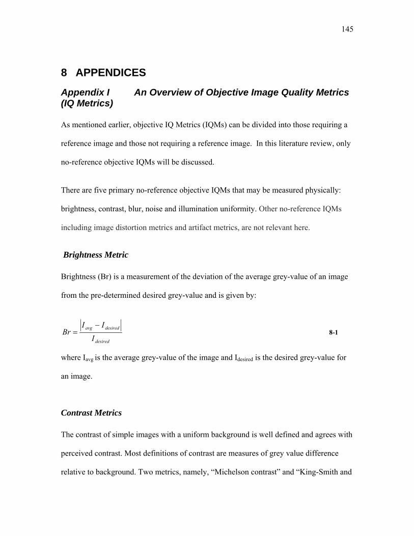
145
8 APPENDICES
Appendix I An Overview of Objective Image Quality Metrics (IQ Metrics) As mentioned earlier, objective IQ Metrics (IQMs) can be divided into those requiring a
reference image and those not requiring a reference image. In this literature review, only
no-reference objective IQMs will be discussed.
There are five primary no-reference objective IQMs that may be measured physically:
brightness, contrast, blur, noise and illumination uniformity. Other no-reference IQMs
including image distortion metrics and artifact metrics, are not relevant here.
Brightness Metric
Brightness (Br) is a measurement of the deviation of the average grey-value of an image
from the pre-determined desired grey-value and is given by:
desired
desiredavg
I
IIBr
−= 8-1
where Iavg is the average grey-value of the image and Idesired is the desired grey-value for
an image.
Contrast Metrics
The contrast of simple images with a uniform background is well defined and agrees with
perceived contrast. Most definitions of contrast are measures of grey value difference
relative to background. Two metrics, namely, “Michelson contrast” and “King-Smith and

146
Kulikowski contrast”, have been commonly used for quantifying contrast. Michelson
contrast is given by
minmax
minmax
LLLLCM +
−= 8-2
where Lmax and Lmin are the maximum and minimum grey values, respectively.
Michelson contrast is a global contrast. It is sometimes not appropriate because one or
two points of extreme brightness or darkness can determine the contrast of the whole
image. In this work, this definition will be used because of its generality without any
assumptions attached and its effectiveness for describing the global contrast of an image.
The King-smith and Kulikowski contrast is given by
LLCkk
Δ= 8-3
where L is the background grey value, and ΔL is the increment or decrement in the object
grey value from the uniform background. One usually assumes a large background with a
small object, in which case the average grey value will be close to the background grey
value. This definition of global contrast requires a uniform background, which is not the
case for most images in this research. However, this definition as a local contrast metric
was used in this research.
The two metrics above assign a single value to the whole image, but contrast may vary
greatly across the image. This is particularly true for complex images with a non-uniform
background. Peli [113] suggested a contrast metric based on a Fourier transformation. For
each frequency band, the contrast is defined as the ratio of the bandpass-filtered image at
that frequency to the low-pass image filtered to an octave below the same frequency

147
(local grey value mean). This definition gives each pixel a contrast measurement and is
given by
),(),(),(
yxlyxayxc = 8-4
where c(x,y) is the contrast at pixel (x,y), a(x,y) is the grey level of pixel (x,y) on an x,y
co-ordinate scale in a band-pass filtered image, and l(x,y) is the grey level of pixel (x,y)
in a low-pass filtered image. This definition provides a local contrast measure for every
spatial frequency that depends not only on the local grey value at that frequency but also
on the local background grey value as it varies from place to place in the images.
However, this definition is computationally expensive even though it does provide a
reliable way to calculating local contrast.
VeldKamp recommended [39] a local contrast metric given by
∑∈
−=)(
1iNbdj
jii yN
yc 8-5
where Nbd(i) represents a neighborhood or window at i of size N, and y is the grey value
of a pixel.
VeldKamp’s local contrast metric is used to estimate the local contrast standard deviation
for different grey levels. However, this metric is only applicable when noise depends
strongly on the intensity. It proved to be successful for mammogram images [114].
For a real-time imaging system, a local contrast metric is more reliable than a global
contrast metrics because the background of image often constantly changes from place to
place in the image.

148
Noise Metrics
Noise is random fluctuation in the grey value of a pixel as opposed to deterministic
distortions, such as shading or lack of focus. It is a defect that can take many forms and
arise from various sources. In most cases it shows up as a sharp variation in grey value in
a uniform region of the scene. Noise can be in the form of photon noise, thermal noise,
readout noise, amplifier noise and quantization noise. Among these, photon noise is a
Poisson noise which is significant in most cases. Other forms of including readout noise,
amplifier noise and quantization noise, are additive (Gaussian) and can be reduced to
manageable levels through image processing. Noise is of high spatial frequency in the
frequency domain.
In general, a pixel is declared to be noisy if it violates the local smoothness constraint
(around an edge area). The most commonly used metric of noise is signal-to-noise ratio
(SNR). SNR can have several definitions. The noise is characterized by its standard
deviation, σn.
If the image (signal) is known to lie between two boundaries, Lmax (max grey value of an
image) and Lmin (minimum grey value of an image), then the SNR in decibles (dB) is
defined as:
dBLLSNRn
)(log20 minmax10 σ
−= 8-6
If the grey value is not bounded but has a statistical distribution then two other definitions
are used. If signal and noise are interdependent, then the SNR is given by

149
dBmSNRn
a )(10log20σ
= 8-7
where ma is sample mean of the pixel grey levels in a region of interest in an image ;
Otherwise when signal and noise are independent, we have
dBSNRn
a )(10log20σσ
= 8-8
where σa is the standard deviation of the grey levels of pixels in a region of interest in an
image.
As can be seen, SNR calculation for the entire image based on above equations is not
directly available because standard deviation of noise σn is, in general, unknown. The
normal estimate of the standard deviation of noise based on standard deviation of grey
levels in an image tends to be larger than the true σn because the variations in the image
grey value are not generally due to noise but to variation in local information. There is no
simple way to estimate σn. However, within a region of an image, there is a way to
estimate the SNR. We can use local σa as σn and the dynamic range (Lmax-Lmin) for the
image to calculate a global SNR. The underlying assumptions are that 1) the signal is
approximately constant in that region and the variation in the region is therefore due to
noise, and, 2) that the noise is the same over the entire image with a standard deviation
given by σa=σn.
A fuzzy noise metric was proposed by Zhang [115] for the measurement of impulse
noise, and it is given by

150
⎪⎩
⎪⎨
⎧
≥−
≤−≤−
−−≤−
=
byxmyxobyxmyxoa
abayxmyxo
ayxmyxoyxf
|),(),(|1|),(),(|||),(),(|
|),(),(|0),( 8-9
where o(x,y) is the grey level of pixel (x,y), a and b are the two pre-determined
parameters, m(x,y) is the median value of the grey level of pixel (x,y)’s neighborhood. If
f(x,y) < Td (Td is given threshold value), pixel (x,y) is not an impulse noise.
Mathematically, this metric is simple. However, the drawback of this metric is that its
calculation requires three predefined parameters, which need to be chosen.
Chen [116] proposed Moran I test for measuring the noise of an image. The Moran
coefficient I (Chuang and Huang 1992) for pixels in an r × c window is calculated as
∑
∑ ∑×
× ×
−
−−= cr
yx
o
cr
nm
cr
yxnmyx
Nfyxf
SfnmffyxfI
),(
2
),( ),()],),(,[(
/]),([
/]),([]),([δ
8-10
where f(x,y) is the grey value of pixel (x,y), f is the mean grey value inside the
window. δ [(x,y),(m,n)]=1 if pixel (x,y) and (m,n) are adjacent, and 0 otherwise, So=
∑∑δ[(x,y),(m,n)] is the number of contiguous pairs in an image and N=r × c is the total
number of pixels. This I value measures the noise of the region under study. The
numerator is a measure of covariance among the pixels and the denominator is a measure
of variance. A higher value of I means more correlation between pixels and less
likelihood that the image is noisy. I = 1 when all pixels have the same grey levels. If the
pixels inside the window are randomly distributed, the random variable I can be
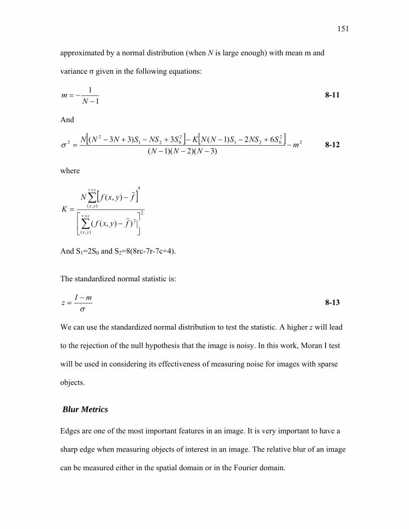
151
approximated by a normal distribution (when N is large enough) with mean m and
variance σ given in the following equations:
11−
−=N
m 8-11
And
[ ] [ ] 22021
2021
22
)3)(2)(1(62)1(3)33(
mNNN
SNSSNNKSNSSNNN−
−−−+−−−+−+−
=σ 8-12
where
[ ]2
),(
2
4
),(
)),((
),(
⎥⎦
⎤⎢⎣
⎡−
−=
∑
∑cxr
yx
cxr
yx
fyxf
fyxfNK
And S1=2S0 and S2=8(8rc-7r-7c+4).
The standardized normal statistic is:
σmIz −
= 8-13
We can use the standardized normal distribution to test the statistic. A higher z will lead
to the rejection of the null hypothesis that the image is noisy. In this work, Moran I test
will be used in considering its effectiveness of measuring noise for images with sparse
objects.
Blur Metrics
Edges are one of the most important features in an image. It is very important to have a
sharp edge when measuring objects of interest in an image. The relative blur of an image
can be measured either in the spatial domain or in the Fourier domain.
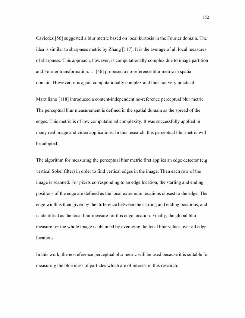
152
Caviedes [50] suggested a blur metric based on local kurtosis in the Fourier domain. The
idea is similar to sharpness metric by Zhang [117]. It is the average of all local measures
of sharpness. This approach, however, is computationally complex due to image partition
and Fourier transformation. Li [46] proposed a no-reference blur metric in spatial
domain. However, it is again computationally complex and thus not very practical.
Marziliano [118] introduced a content-independent no-reference perceptual blur metric.
The perceptual blur measurement is defined in the spatial domain as the spread of the
edges. This metric is of low computational complexity. It was successfully applied in
many real image and video applications. In this research, this perceptual blur metric will
be adopted.
The algorithm for measuring the perceptual blur metric first applies an edge detector (e.g.
vertical Sobel filter) in order to find vertical edges in the image. Then each row of the
image is scanned. For pixels corresponding to an edge location, the starting and ending
positions of the edge are defined as the local extremum locations closest to the edge. The
edge width is then given by the difference between the starting and ending positions, and
is identified as the local blur measure for this edge location. Finally, the global blur
measure for the whole image is obtained by averaging the local blur values over all edge
locations.
In this work, the no-reference perceptual blur metric will be used because it is suitable for
measuring the blurriness of particles which are of interest in this research.
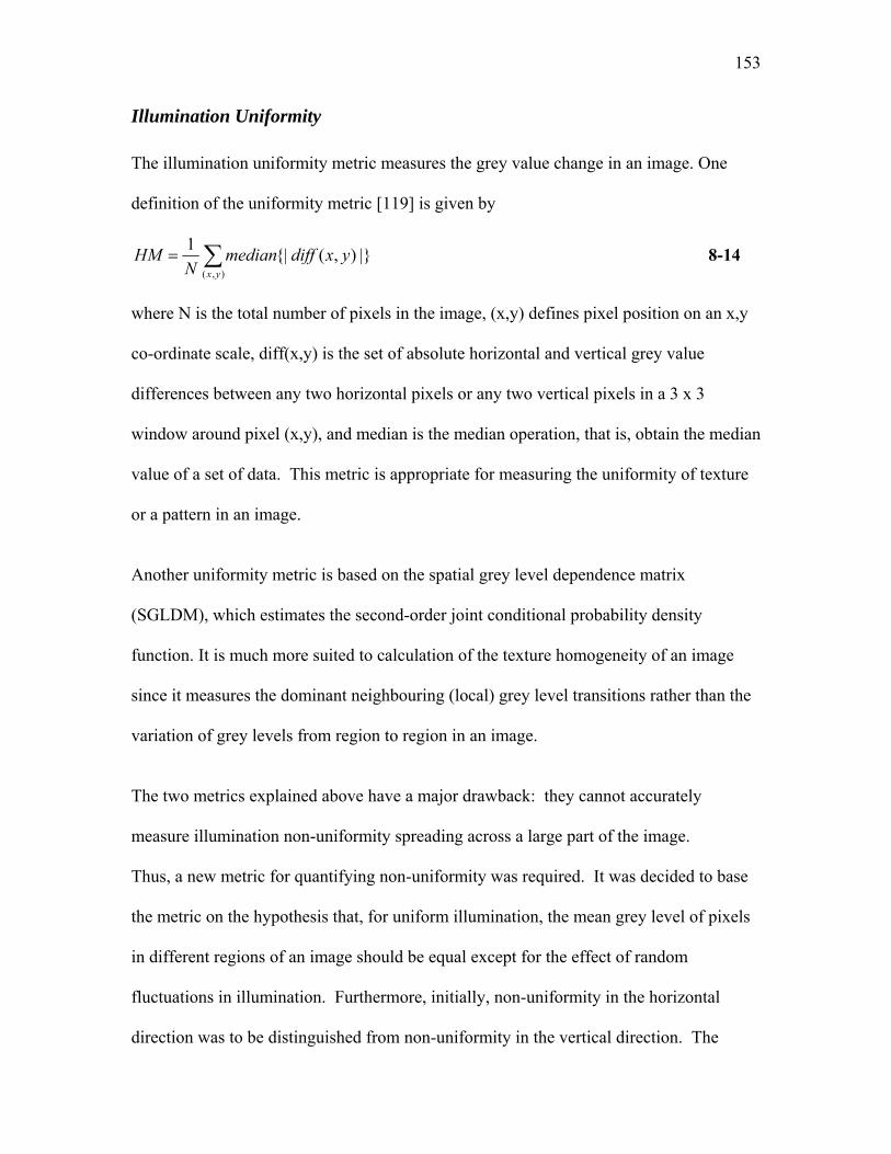
153
Illumination Uniformity
The illumination uniformity metric measures the grey value change in an image. One
definition of the uniformity metric [119] is given by
∑=),(
|}),({|1yx
yxdiffmedianN
HM 8-14
where N is the total number of pixels in the image, (x,y) defines pixel position on an x,y
co-ordinate scale, diff(x,y) is the set of absolute horizontal and vertical grey value
differences between any two horizontal pixels or any two vertical pixels in a 3 x 3
window around pixel (x,y), and median is the median operation, that is, obtain the median
value of a set of data. This metric is appropriate for measuring the uniformity of texture
or a pattern in an image.
Another uniformity metric is based on the spatial grey level dependence matrix
(SGLDM), which estimates the second-order joint conditional probability density
function. It is much more suited to calculation of the texture homogeneity of an image
since it measures the dominant neighbouring (local) grey level transitions rather than the
variation of grey levels from region to region in an image.
The two metrics explained above have a major drawback: they cannot accurately
measure illumination non-uniformity spreading across a large part of the image.
Thus, a new metric for quantifying non-uniformity was required. It was decided to base
the metric on the hypothesis that, for uniform illumination, the mean grey level of pixels
in different regions of an image should be equal except for the effect of random
fluctuations in illumination. Furthermore, initially, non-uniformity in the horizontal
direction was to be distinguished from non-uniformity in the vertical direction. The

154
approach used was essentially a two way analysis of variance (ANOVA). The image was
divided into equal regions (actually segments of 50 X 50 pixels as shown in Figure 8-1).
In Figure 8-1, the treatment variable (vertical direction) has 6 levels (T1~T6) and the
block variable (horizontal direction) has 7 levels (B1~B7). . The grey levels of pixels are
considered as replicates at specific treatment and block levels. Within each region the
grey level variability is assumed to follow a Normal distribution with the same standard
deviation in each.

155
Figure 8-1 Quantification of Illumination Uniformity Using ANOVA Analysis The two-way ANOVA table Table 8-1 shows how the usual ANOVA F statistics were
calculated where “a” is the number of horizontal levels, “b” is the number of vertical
levels, n is the sample size (number of pixels) for each segment, N (= abn) is the total
sample size (total number of pixels in an image).
50 pixels
Treatment (i)
Block (j) B1 B2 B3 B4 B5 B6 B7
T1
T2
T3
T4
T5
T6

156
Table 8-1 Two-way ANOVA Table for Quantifying the Illumination Uniformity
Source of Variances
Sum of Square (SS)
Degree of Freedom
(df)
Mean Sum of Square(MSS)
Calculated F Value
Critical F
Value Horizontal Effect (H)
SS(H) a-1 MSS(H) =SS(H)/(a-1)
F(H)= MSS(H)/MSS(E)
Fcritical,(H)
Vertical Effect (V)
SS(V) b-1 MSS(V)= SS(V)/(b-1)
F(V)= MSS(V)/MSS(E)
Fcritical(V)
Interaction Effect
SSI (a-1)(b-1) MSS(I)= SSI/((a-1)(b-1))
FI= MSS(I)/MSS(E)
Fcritical(HV)
Within (error)
SSE ab(n-1) MSS(E)= SSE/(ab(n-1))
Total TSS abn-1 Note: Fcritical(H) is the critical F value with degrees of freedom of a-1, ab(n-1) and
significance level at 5%; Fcritical(V) is the critical F value with degrees of freedom of b-1, ab(n-1) and
significance level at 5%; Fcritical(HV) is the critical F value with degrees of freedom of (a-1)(b-1), ab(n-1)
and significance level at 5%. The calculation of SS(H), SS(V), SSI, TSS and SSE in Table 8-1 is given by the
following equations and in that order:
∑=
−=a
ii xxnbHSS
1
2)()( 8-15
∑=
−=b
jj xxnaVSS
1
2)()( 8-16
∑∑= =
+−−=b
j
a
ijiij xxxxnSSI
1 1
)( 8-17
∑∑∑= = =
−=n
k
b
j
a
ikji xxTSS
1 1 1)( 8-18
SSIVSSHSSTSSSSE −−−= )()( 8-19
where x is the mean grey value of the image, ix is the mean grey value of ith horizontal
row in the segmented image, jx is the mean grey value of the jth vertical column in the
segmented image, ijx is the mean grey value of the segment at the ith row and jth column

157
in the segmented image, and kjix is the grey value of the kth pixel in the segment of the ith
row and jth column.
The above analysis permits uniformity of illumination to be assessed in both a horizontal
and a vertical direction. However, it was found that assessment in only the horizontal
direction was sufficient. An illumination uniformity metric (IU) was defined as follows:
)()(
)()(
1)()(
HFHFIU
HFHFif
IUHFHFif
critical
critical
critical
=
>
=<=
8-20
That is, if the calculated (observed) F value (F(H)) of the horizontal effect is less than or
equal to the critical F value (Fcritical(H)) at a 5% significance level, the illumination
uniformity is unity. This is equivalent to accepting the null hypothesis that the mean grey
values at different locations in the horizontal direction of an image are the same;
otherwise the illumination uniformity metric is calculated as the ratio of critical F value
to the calculated F value. Thus, the metric quantifies how closely the calculated F value is
to the critical F value: the worse is the illumination uniformity of an image, the lower the
measured value of this illumination uniformity metric. It is expected that the usual
ANOVA assumptions (Normal distribution of grey levels and identical standard
deviations in each region) could sometimes be invalid, especially when a large particle is
located in a region for example. However, results are quite robust to such violations
(http://www.statsoft.com/textbook/stanman.html#assumptions ) except if the variance for

158
each region is correlated with the mean value. This was not found to be the case here for
various images examined. However, the ultimate test is whether the use of the IU metric
agrees with observed uniformity, whether it shows improvement when uniformity is
improved and whether it enables image quality to be modified for improved
classification. Table 8-2 shows the values of IU for 745 “typical images” before and after
correction of uniformity. Values agreed with subjective evaluation of image uniformity.
Also, the average value of illumination uniformity for the raw images is 0.017: This was
much lower that the average of 0.89 for the illumination corrected images. Furthermore,
it was demonstrated that each illumination corrected image had a higher illumination
uniformity value than did its raw image. Based upon these results the IU metric was used
throughout the thesis for quantifying image uniformity with the classification results
provided additional justification for its use.
Table 8-2 Comparison of Illumination Uniformity for Raw Images and Their Illumination Corrected Images
Illumination Uniformity 745 Raw Images 745 Illumination Corrected
Images Average Value 0.017 0.89
Minimum Value 0.005 0.18 Maximum Value 0.076 1
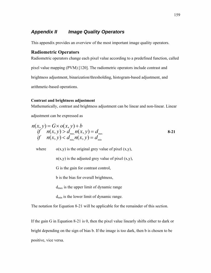
159
Appendix II Image Quality Operators This appendix provides an overview of the most important image quality operators.
Radiometric Operators Radiometric operators change each pixel value according to a predefined function, called
pixel value mapping (PVM) [120]. The radiometric operators include contrast and
brightness adjustment, binarization/thresholding, histogram-based adjustment, and
arithmetic-based operations.
Contrast and brightness adjustment Mathematically, contrast and brightness adjustment can be linear and non-linear. Linear
adjustment can be expressed as
minmin,
maxmax,
),(),(),(),(
),(),(
dyxndyxnifdyxndyxnif
byxoGyxn
=<=>
+×= 8-21
where o(x,y) is the original grey value of pixel (x,y),
n(x,y) is the adjusted grey value of pixel (x,y),
G is the gain for contrast control,
b is the bias for overall brightness,
dmax is the upper limit of dynamic range
dmin is the lower limit of dynamic range.
The notation for Equation 8-21 will be applicable for the remainder of this section.
If the gain G in Equation 8-21 is 0, then the pixel value linearly shifts either to dark or
bright depending on the sign of bias b. If the image is too dark, then b is chosen to be
positive, vice versa.
160
When constraints are put on o(x,y) in Equation 8-21, the contrast and brightness
adjustment can be piecewise linear, and this is given by
minmin,
maxmax,
),(),(),(),(
),(),(),(
dyxndyxnifdyxndyxnif
UyxoLbyxoGyxn
=<
=><<
+×=
8-22
where L and U are constants between dmax and dmin.
In Equation 8-22, the choice of L and U has a strong effect on contrast enhancement.
When L and U are in the lower range of dynamic range, the contrast is stretched in the
dark range, that is, the contrast in the low grey level are enhanced which is useful if the
contrast is poor in the dark range. When L and U are in the upper range of dynamic
range, the contrast is stretched in the light range.
Other than linear adjustments, there are non-linear adjustments such as logarithmic
adjustment useful for x-ray images, and exponential adjustment.
Techniques based on Image Histogram
The histogram of an image counts the number of occurrences of each possible value. Sum
of all values in the histogram gives us the total number of pixels in image, and this is
given by (if grey value is assumed continuous):
∫= max
min
)(d
ddDDHA 8-23
where H(D) is the count of pixels with grey value of D, and
A is the total number of pixels in an image;
161
The probability density of a grey value is calculated by normalizing the histogram, i.e.,
ADHDp )()( = 8-24
where p(D) is the probability density of the pixels with grey value of D.
The cumulative density of a grey value is computed by integrating probability density
∫=D
ddDDpD
min
)()(ω 8-25
In addition, a cumulative histogram for an image can be computed as follows:
∫=D
ddaaHDC
min
)()( 8-26
where C(D): the cumulative count of all pixels with grey value up to D (inclusive).
There are two commonly used histogram-based techniques: histogram matching and
histogram equalization.
Histogram Matching
Histogram matching is obtaining an image whose histogram has a specific shape.
Mathematically this is given by
)),(()),((arg yxoCyxnC originalett = 8-27
where Ctarget is the cumulative count of pixels with a new grey value of n(x,y), Coriginal is
the cumulative count of pixels with a grey value of o(x,y).
Histogram Equalization

162
The objective of histogram equalization is to enhance image contrast by flatting the
image histogram and increasing the dynamic range dramatically without affecting the
structural information. Mathematically it is given by
)),((),( yxoCyxn original= 8-28
Histogram equalization may not always produce desirable results, especially for images
with a very narrow histogram and relatively few grey levels. It can produce false edges
and regions. The equalized image may look unnatural, e.g., increased visual graininess. In
some cases, contrast stretching works better since it can work on a selected region of
dynamic range.
Binarization/thresholding
Binarization is an extremely important image processing operation. Its objective is to
separate image background from the foreground. Single threshold binarization is given by
⎩⎨⎧
>≤
=TyxoifTyxoif
yxn),(255),(0
),( 8-29
where T is the threshold value.
Double threshold binarization is given by
⎩⎨⎧
<>≤≤
=21
12
),(),(255),(0
),(TyxoorTyxoif
TyxoTifyxn 8-30
where T1 and T2 are the lower and upper thresholds.
Notwithstanding its apparent simplicity, binarization is a very difficult problem because
of the choice of threshold. A number of conditions can make binarization difficult: poor

163
image contrast, spatial non-uniformity in background intensity, and the ambiguity of
image foreground and background due to multiple levels of different objects.
There is not a single optimally suited method of binarization for all images. Different
approaches for binarization should be taken for images with different characteristics. It is
often best to make the decision by experimentation.
Two categories of binarization techniques are used [121]: global thresholding and locally
adaptive thresholding. Global thresholding techniques use the histogram to identify a
threshold between foreground and background grey values. A single threshold is
determined by treating each pixel value independently of its neighborhood, or without
context. Locally adaptive techniques examine relationship between grey values of
neighboring pixels to adapt the threshold according to the prevailing grey value statistics
for different image regions. Adaptive techniques are applied in an attempt to counter the
effects of nonuniformities in image background.
For images with uniform background, the optimal global techniques ensure better
binarization than the locally adaptive techniques because for global techniques, threshold
selection is based on a larger data set of pixels. Also, for adaptive techniques, a size
parameter matching the size of uniform background regions must be chosen.
ISODATA
A popular global thresholding algorithm is the ISOData based on the histogram. The
ISOData is a simple single value global thresholding method. It is given by
TmmT rightleft −=− 8-31

164
where mleft is the mean value of all grey values with value less than or equal to T in the
histogram and mright is the mean value of all grey values greater than T in the histogram.
Note that both mleft and mright are function of T.
The ISODATA performs well when there are two clearly resolved peaks in the
histogram. Where there are multiple peaks in the histogram, double value thresholding in
general works better than single value thresholding.
There are a set of optimal thresholding techniques based on criterion functions measuring
the separation between regions. For these methods, a criterion function is calculated for
each grey value and that which maximizes/minimizes this function is chosen as the
threshold. These methods include Ostu’s discriminant method, entropy maximization,
moment preservation and minimum error thresholding.
Discriminant method
The discriminant method is a classic global thresholding method. The criterion function
used in this method is
2
2
t
b
δδη = 8-32
where δb2 is the between-classes (between-peaks) variance, and δt
2 is the total variance
with respect to threshold T. The grey value maximizing the criterion function is the
optimal threshold. Between-peaks variance is defined as
22121
2 )( μμωωδ −=b 8-33
where ω1, ω2, µ1, µ2 are the cumulative probabilities and mean values for each class,
respectively.
165
Entropy maximization
In entropy maximization, entropy is used to measure the separation of two classes. This
method entails separating the image data into two classes, above and below a threshold,
and measuring the entropies of each class. This separation is done for each grey value,
and that value for which the sum of entropies of two classes is maximum is the optimal
threshold. The criterion function is given by
∑∑+==
+−=255
10
))(log()())(log()((Ti
T
i
ipipipipE 8-34
In Equation 8-34, the probability p(i) is calculated only within the class.
Moment Preservation
In moment preservation, moments are first calculated for the original image. Next, they
are calculated for images thresholded by every grey value. The threshold value at which
the original and the thresholded images have closest moments is the optimal threshold.
The total moment of the thresholded image is given by
∑∑+==
×+×255
1
4
0
4 )()(Ti
T
i
iipiip 8-35
In Equation 8-35, the probability p(i) is calculated only within the class.
Minimum Error Thresholding
This method assumes that the histogram is composed of two normally distributed classes
of pixel grey values. Two normal distribution curves are determined by an iterative
process to fit the two classes of pixels in the histogram and minimize a specified
classification error. A prospective threshold value is tested on each iteration by

166
calculation of the means and the variances from the histogram for the two classes
separated by this threshold. The threshold minimizing the error is the optimal threshold.
Region Averaging
Region averaging is a local adaptive technique. It is very useful for image with varying
background. It is implemented by first calculating a running region average, by
comparing each pixel value to its local average, and setting that value to either the
foreground, if it is much above the average, or to the background, if it is much below. In
cases in which the difference between the pixel value and its local average is small, the
pixel value stays unchanged. The region size for calculating the local average should
reflect the size of expected foreground features; it should be large enough to enclose a
feature completely, but not so large as to average across background non-uniformity. The
choice of proper region size may be problematic when the sizes of foreground features in
the image vary dramatically.
Subimage Thresholding Subimage thresholding is desirable for images with a high degree of background non-
uniformity. Depending on the degree of background non-uniformity, a N x M image is
partitioned into N/n x M/m subimages of size n x m. Optimal thresholds are determined
within each subimages using global thresholding techniques. Any subimage with a small
measure of class separation is considered to contain only one class, and its threshold is
taken as the average of the thresholds in the neighboring subimages. Finally, the
subimage thresholds are interpolated among subimages for all pixels and each pixel is
binarized with respect to the threshold at the pixel.

167
Arithmetic-based operations
This is a group of operations that are not very widely used. Mathematically they are given
by
)),((),( yxoyxn φ= 8-36
where φ is an abstraction of one of the following arithmetic operations including: add a
constant, subtract a constant, multiply a constant, divide a constant, min, max, binary OR,
binary XOR, Gamma, log, square, square root and reciprocal and so on. For addition and
subtraction operation, the effect is the same as brightness adjustment; for multiplication
and division, the effect is similar to contrast stretching or shrinking. Other operations are
not used often and will not be discussed here.
Geometric Operators
Geometric operators change each pixel value according to a function which takes into
account the neighborhood of the pixel. The function, which could be linear or non-linear,
is called a filter. There are two types of filters: smoothing filters which remove additive,
impulsive and speckle noise, and sharpening filters which remove motion induced or
defocused blurs and sharpen edges. For most of the filters, a neighborhood window with
an appropriate size is chosen. The shape of window can be square, rectangular, plus ‘+’
or cross ‘x’.
Mean filter
The grey value of a pixel is assigned to the mean value of its neighbors. A mean filter is
used to smooth and remove noise. Mathematically it is given by

168
Nbd
jimyxn yxNbdji
∑∈= ),(,
),(),( 8-37
where Nbd is the number of neighborhood pixels of pixel (x,y),
Nbd(x,y) is the neighborhood of pixel (x,y),
M(i,j) is the grey value of pixel (i,j).
For a neighborhood of k x k, the filter length is k. The rule of thumb for practical mean
filters is to set filter length k=2D+1 pixels to blur objects with diameter D or smaller.
This filter of length k will reduce any feature of characteristic size small than D.
Conversely, if one wished to retain all image features of diameter D or above, a suitable
choice would be k <= 2D-1.
The fact that the mean filter is limited to the adjustment of its length to control
performance has some drawbacks. First, while speckle noise may be reduced
substantially, important image features such as edges and textures may be equally
affected and thus blurred if features and noise exhibit similar degrees of acuity. This is a
fundamental problem of all low-pass filtering, but it is particularly severe for the mean
filter. Closely related is a second problem of the mean filter, namely its propensity to
introduce a ringing distortion. These problems can be prevented by use of a filter whose
coefficients, rather than exhibiting a sharp drop, gradually decrease to zero at the edges as
the weighted mean filter and Gaussian filter do.
Weighted mean filter
The weighted mean filter is different from mean filter in that the grey value of a pixel is
assigned to the weighted mean value of its neighborhood pixels rather than the mean
169
value of its neighbors. A neighboring pixel of a pixel is weighted according to its spatial
distance from the pixel. The effect of weighted mean filter is smoothing and removing
noise. But the smoothing effect is less than mean filter in general. The filter is given by
Nbd
jimjiwyxn yxNbdji
∑∈
×= ),(,
),(),(),( 8-38
where w(i,j) is the weight assigned to pixel (i,j).
Mode filter
The mode filter is non-linear filter according to order statistics. The grey value of a pixel
is replaced by the grey value of its most common neighbor. This is given by
)),(),(|),((emod),( yxNbdjijimyxn ∈= 8-39
The mode filter is suitable to remove isolated noise.
Median Filter
The median filter is a non-linear filter according to order statistics. The grey value of a
pixel is replaced by the median value of its neighbors. The filter is given by
)),(),(|),((median),( yxNbdjijimyxn ∈= 8-40
The advantage of the median filter is that it removes impulsive noise while preserve
edges. The median is a more robust average than the mean filter because a single very
unrepresentative pixel in a neighborhood will not affect the median value significantly.
Since the median value must actually be the value of one of the pixels in the
neighborhood, the median filter does not create new unrealistic pixel values when the

170
filter straddles an edge. For this reason the median filter is much better at preserving
sharp edges than the mean filter.
It is computationally expensive since it needs sorting the neighbors. When the window
size k is big, the sorting is even more time-consuming.
Closest of Minimum and Maximum
The grey value of a pixel is set to the minimum or maximum of its neighbors depending
on which one is closest to its grey value. This filter can sharpen boundaries between
textures. It is given by
)),(,|),()),(max(||,),()),(min(min(|),(
yxNbdjiyxojimyxojimyxn
∈−−=
8-41
Minimum
This filter does grayscale dilation by replacing the grey value of each pixel in the image
with the smallest grey value in that pixel's neighborhood.
)),(),(|),(min(),( yxNbdjijimyxn ∈= 8-42
This filter increases the size of objects which are darker than background.
Maximum
This filter does grayscale erosion by replacing the grey value of each pixel in the image
with the largest grey value in that pixel's neighborhood.
)),(),(|),(max(),( yxNbdjijimyxn ∈= 8-43 This filter decreases the size of objects which are lighter than background.
K-Nearest Neighbors

171
The grey value of pixel (x,y) is set to the average of the k pixels in its neighbors whose
values are closest to o(x,y). A typical value of k =6 is chosen for 3 x 3 square filter.
k
jimyxn yxKNNji
∑∈= ),(,
),(),( 8-44
where KNN(x,y) is the k nearest neighbors of pixel (x,y).
K-Nearest Neighbors filter can smooth image while preserving edges.
Unsharp Masking
Unsharp masking consists of a series of operations. First, the original image is blurred.
Next, a mask is obtained by subtracting blurred image from the original image. Finally
the mask is added to the original image forming the resulting image. Unsharp masking
can enhance small features while large features are suppressed. Mathematically unsharp
masking is given by
))),((),((),(),( yxobluryxoyxoyxn −+= η 8-45
where η is scaling factor.
There are two control parameters in unsharp masking: the window size for blurring
operation and the scaling factor of the mask. The larger the scaling factor, the sharper the
edge will be. The degree of blurring controls what sized edges the unsharp mask
functions on most effectively. Larger stronger blurs produce masks that alter larger edges
but miss smaller edges, while small subtle blurs capture tiny sudden edges but miss larger
edges.
Laplacian Edge Sharpening
172
In Laplacian edge sharpening, the resulting image is obtained by subtracting a multiple of
the Laplacian from the blurred image. The image is blurred by Laplacian operation
2
2
2
22 ),(),(),(
yyxo
xyxoyxo
∂∂
+∂
∂=∇ 8-46
),(),(),( 2 yxoyxoyxn ∇−= β 8-47
where β is a constant.
The advantage of Laplacian edge sharpening is that features in any direction are
sharpened equally.
Filling Operator
The filling operator is a noise filter for binary (black and white) images. Noise in binary
images takes the form of isolated ON pixels, or pixel regions, in a background of OFF
pixels, or vice versa. ON pixels are black with grey value equal zero while OFF pixel are
white with grey value 1. This type of noise is called salt-and-pepper noise, which can be
removed by filling operator. With filling operator, each isolated noise is filled in by the
grey value of its neighbor.
The most common practice of binary noise reduction is to use a filling mask. A filling
mask of 3 x 3 is sliding through the image. When the grey value of the center pixel is not
equal to the grey value of all its surrounding pixels, the center pixel grey value is
assigned with the grey value of its neighbors.

173
However, this simple technique only removes single pixel noise while larger noise
features will remain intact, particularly for those noise features at the edge of a region as
bulges or concaves.
A more general filter, called kFill, is designed to reduce isolated noise and noise on
contours up to a selected limit in size. The k of kFill refers to a size adjustment
parameter. Other kFill parameters can be set to control rounding of the filtered features.
Many shapes display 90oC corners: To preserve these, rounding must be minimized, and
the default parameters of kFill are chosen accordingly to retain corners of 90oC or
greater.
Filling operations are performed for each image pixel using a k x k window. This window
is composed of an interior (k-2) x (k-2) region, the core, and the exterior 4(k-1)
neighborhood pixels. All values of the core are set to ON or OFF, depending on pixel
values in the neighborhood.
Whether to fill with ON or OFF requires that all core pixels to be OFF or ON,
respectively. It also depends on three variables, n, c and r, which are determined from the
neighborhood pixels. Parameter n equals the number of ON (OFF) pixels in the
neighborhood, c denotes the number of connected groups of ON pixels in the
neighborhood, and r represents the number of corner pixels that are ON (OFF). In the
default implementation, filling occurs when the following logic conditions are met:
[ ])2)43(()43(1 =∧−=∨−>∧= rknknc where
∧ is logic AND operator, and ∨ is logic OR operator;
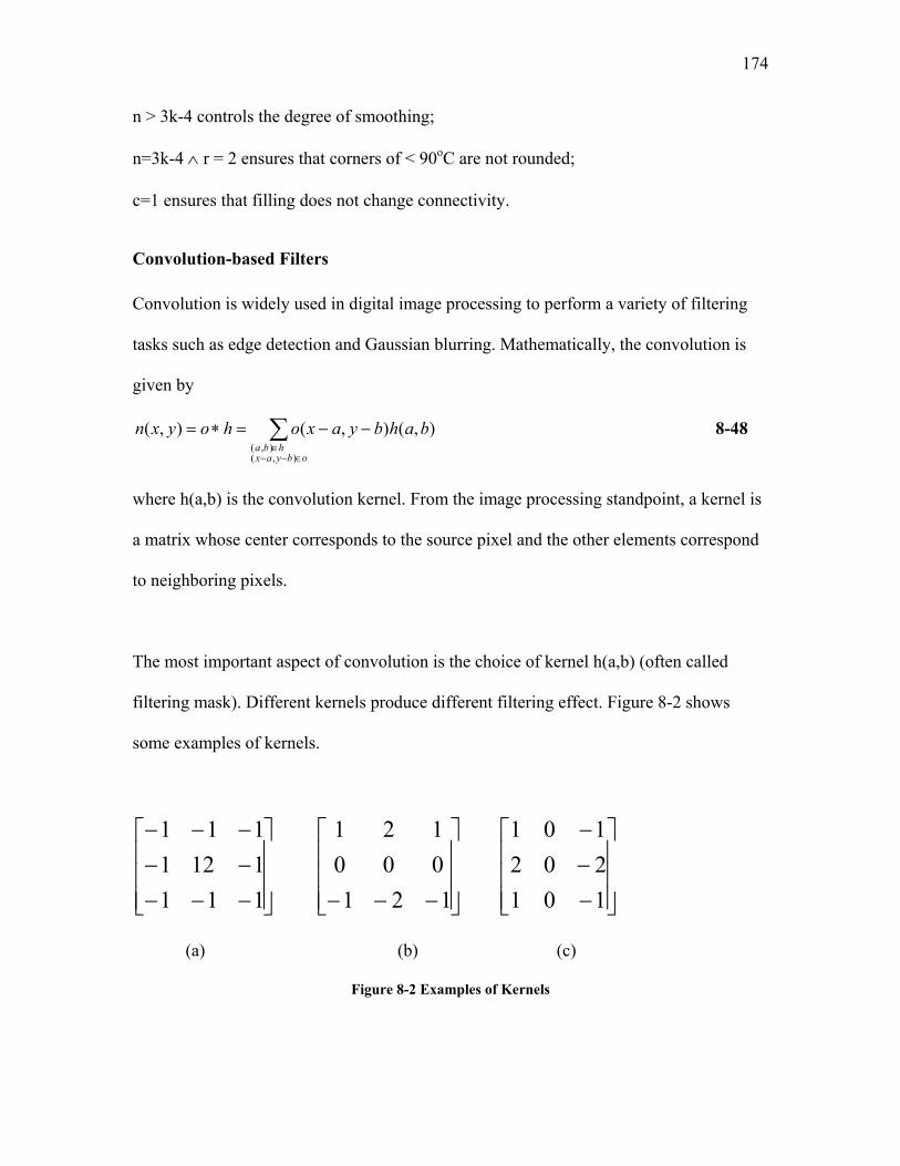
174
n > 3k-4 controls the degree of smoothing;
n=3k-4 ∧ r = 2 ensures that corners of < 90oC are not rounded;
c=1 ensures that filling does not change connectivity.
Convolution-based Filters
Convolution is widely used in digital image processing to perform a variety of filtering
tasks such as edge detection and Gaussian blurring. Mathematically, the convolution is
given by
∑∈−−
∈
−−=∗=
obyaxhba
bahbyaxohoyxn),(
),(),(),(),( 8-48
where h(a,b) is the convolution kernel. From the image processing standpoint, a kernel is
a matrix whose center corresponds to the source pixel and the other elements correspond
to neighboring pixels.
The most important aspect of convolution is the choice of kernel h(a,b) (often called
filtering mask). Different kernels produce different filtering effect. Figure 8-2 shows
some examples of kernels.
⎥⎥⎥
⎦
⎤
⎢⎢⎢
⎣
⎡
−−−−−−−−
1111121111
⎥⎥⎥
⎦
⎤
⎢⎢⎢
⎣
⎡
−−− 121000121
⎥⎥⎥
⎦
⎤
⎢⎢⎢
⎣
⎡
−−−
101202101
(a) (b) (c)
Figure 8-2 Examples of Kernels
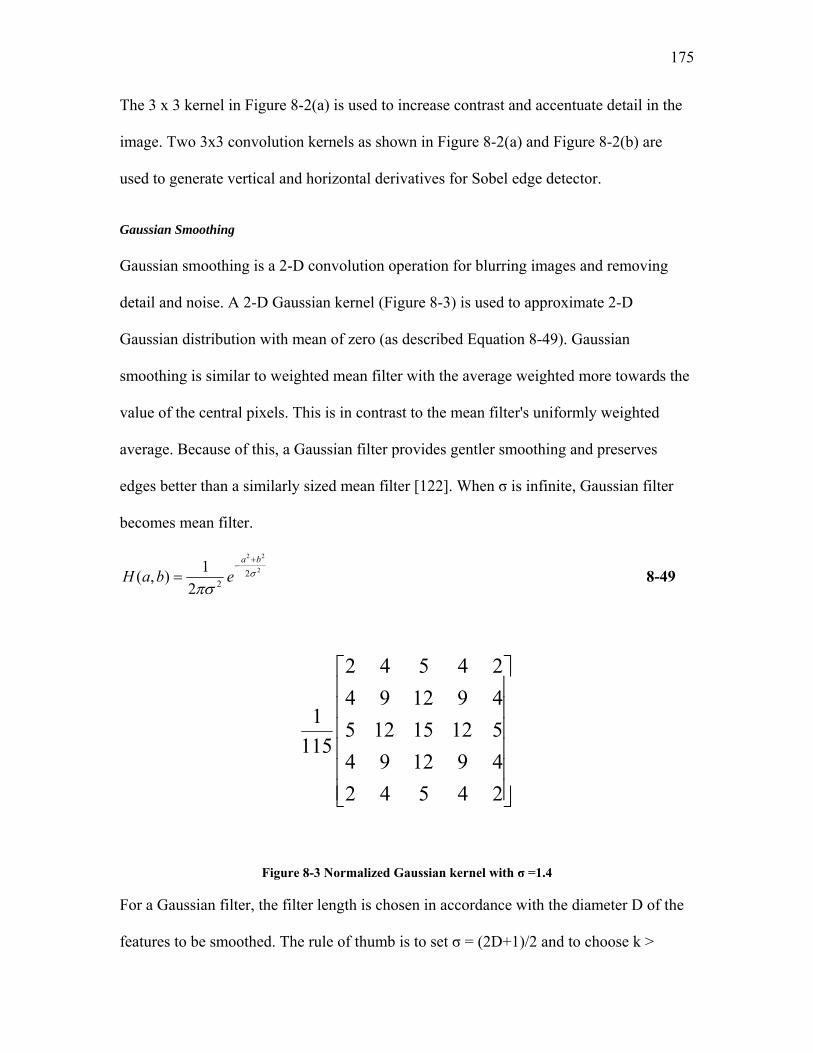
175
The 3 x 3 kernel in Figure 8-2(a) is used to increase contrast and accentuate detail in the
image. Two 3x3 convolution kernels as shown in Figure 8-2(a) and Figure 8-2(b) are
used to generate vertical and horizontal derivatives for Sobel edge detector.
Gaussian Smoothing
Gaussian smoothing is a 2-D convolution operation for blurring images and removing
detail and noise. A 2-D Gaussian kernel (Figure 8-3) is used to approximate 2-D
Gaussian distribution with mean of zero (as described Equation 8-49). Gaussian
smoothing is similar to weighted mean filter with the average weighted more towards the
value of the central pixels. This is in contrast to the mean filter's uniformly weighted
average. Because of this, a Gaussian filter provides gentler smoothing and preserves
edges better than a similarly sized mean filter [122]. When σ is infinite, Gaussian filter
becomes mean filter.
2
22
222
1),( σ
πσ
ba
ebaH+
−= 8-49
⎥⎥⎥⎥⎥⎥
⎦
⎤
⎢⎢⎢⎢⎢⎢
⎣
⎡
245424912945121512549129424542
1151
Figure 8-3 Normalized Gaussian kernel with σ =1.4
For a Gaussian filter, the filter length is chosen in accordance with the diameter D of the
features to be smoothed. The rule of thumb is to set σ = (2D+1)/2 and to choose k >
176
2D+1. In practice, either k=2D+3 or k = 2D+5 is common. A larger value of k ensures
less ringing, but require more computation.
The Gaussian filter requires more computation time than a mean filter to accomplish the
same amount of smoothing, given that the Gaussian filter exceeds the size of the
equivalent uniform filter and contains coefficients of several values and hence requires
multiplication (in contrast to simple addition for the mean filter) for performing the
convolution operation.
Edge Detector
The objective of edge detector is to find the edges of objects in an image. With the
detection of edges of an object, the object can be isolated and further analysis can be
performed. Many edge detectors use the idea of calculating spatial gradient on an image.
These edge detectors include Robert cross, Sobel edge detector, and Canny edge detector.
Canny edge detector is considered to be an optimal one. The Canny operator works in a
multi-stage process. First of all, the image is smoothed by Gaussian smoothing. Then a
simple 2-D first derivative operation is applied to the smoothed image to highlight
regions of the image with high first spatial derivatives.
Mathematical Morphological Operators
Morphological operators refer to a class of spatial filtering operations that are applied to
change the shape of a region in a binary image. That is, morphological operations replace
the binary value at a single pixel location by a value computed from the pixels values
within a neighborhood of chosen shape and size around that location.
177
The most basic morphological operations are erosion and dilation. Erosion is the
reduction in size of ON regions. (ON-valued pixel is black, and OFF-valued pixel is
white). This is more readily accomplished by iterative peeling of single-pixel layers from
the outer boundary of all ON regions. Dilation is the opposite process. Both operations
are usually applied iteratively to erode or dilate by many layers. An example for the
application of erosion is the removal of a layer, one or two pixels wide, of noisy
boundary pixels in a binary image. The analogous dilation process can be applied to fill
holes or to join disconnected lines with gaps up to two pixels in width.
Morphological operations are commonly used for noise reduction and feature detection,
with the objective that noise be reduced as much as possible without eliminating essential
features.
Morphological operations need a mask called structuring element. Structuring element is
similar to a filter mask S(i,j) of size K1 x K2 in which the coefficients take binary values.
Unlike filter masks, a structuring element need not be symmetric, and its origin must be
explicitly labeled. We apply a morphological operation to a pixel by first placing the
designated origin of the structuring element S at that pixel. S defines a neighborhood
Nbd(x,y) of the pixel (x,y).
Erosion
When a structuring element is put over a region, an ON pixel at the origin is set to OFF if
the structuring element does not completely overlap ON-valued pixels of this region.
Erosion is given by
178
⎪⎪⎩
⎪⎪⎨
⎧
∈=−−
=
=
otherwiseOFFyxNbdjiallfor
ONyjxiSjiIANDONyxIifON
yxI),(),(
),(),(),(
),(I 8-50
Dilation
When a structuring element is put over a region, an OFF pixel at the origin is set to ON if
any of the structuring element overlaps ON pixels of the region.
⎪⎪⎩
⎪⎪⎨
⎧
∈=−−
=
=
otherwiseOFFyxNbdjianyfor
ONyjxiSjiIORONyxIifON
yxI),(),(),(),(
),(
),(I 8-51
Opening and Closing
The opening operation involves the application of erosion followed by dilation. The
effect of using a square- or disk-shaped structuring element for opening is to smooth
boundaries, to break narrow isthmuses, and to eliminate small noise regions. The closing
operation is to smooth boundaries, to join narrow break, and to fill small holes. Opening
is used when the images has small noise regions, not used for narrow regions where there
is chance that the initial erosion might disconnect regions. Opening also will eliminate
long or thin features. Closing is used when a region has become disconnected and there is
a need to restore connectivity. It is not used when different regions are located closely
such that the first iteration of dilation might connect them.
Other morphological considerations and operations
179
The choice of the size of the structuring element S and that of the number of iterations
represents a trade-off between the feature size and the number of required iterations. The
larger the size, the fewer the number of iterations, but more computation will be required
on a single iteration. The most common sizes range between 3 x 3 and 5 x 5. The size of
S should be no larger than the features.
Opening tends to eliminate ON-valued noise, while closing will reduce OFF-valued noise
(holes) but smooth sharp features such as corners. Preliminary testing on representative
images is usually necessary to determine a compromise between noise reduction and
feature retention.
Non-uniform Illumination Correction
Nonuniformities in scene illumination are very common in images. Significant spatial
nonuniformities in the illumination introduce bias into the intensity histogram and in turn
interfere with subsequent global image processing operators such as binarization.
Nonuniform illumination correction can be achieved by applying an operation known as
flat fielding. This involves the division of the original by the reference image showing the
slow background variations (but not the objects of interest). Unless otherwise available,
for example, in the form of a separately stored image of the scene background, a
reference image is often created from the original by low-pass filtering such as Gaussian
smoothing with relatively large filter length.
180
Appendix III The Nelder-Mead Simplex Method The Nelder-Mead simplex method was introduced by Nelder and Mead for function
minimization [123] for a system with many variables. It is a systematic direct
optimization method very suitable for problems with a large search space such as
experiments involving many variables. It has advantages over traditional optimization
methods such as the one-variable-at-a-time approach and factorial designs in that it
requires fewer experiments to reach the optimum. It makes no assumptions about an
underlying model and requires no derivatives. As a result, it is simple, easy to implement
and efficient. Simplex methods are adaptive and evolutionary in the sense that they are
sequential, subsequent trials move away from the poorest performance vertices and move
in the direction of improvement. Its progress is based upon a relative ranking of the
values of the objective functions for different values of the parameters.
The simplex method was originally mainly used in analytical chemistry [124]. Over the
years, it gained popularity for various technical system optimization problem such as
process control [125] . There are basically two broad versions of simplex methods: basic
simplex method by Spendley et al and modified simplex methods [125]. Modified
simplex methods are further divided into modified simplex ( Nelder-Mead simplex),
super modified[126], weighted centroid [127] and composite modified [128]. In this
appendix, emphasis will be on the basic simplex method and the Nelder-Mead simplex
method.
Basic Simplex Method
181
A simplex is a geometric figure having a number of vertices equals to one more than the
number of variables in a system, that is, a simplex is defined by k+1 vertices for k
variables. In an optimization process, each vertex represents a set of values for all
variables.
For a two-variable optimization problem, the basic simplex method starts with three
initial trials (vertices), that is, the first simplex consists of three trials. After the initial
trials, the simplex process is sequential, with the addition and evaluation of one new trial
at a time. The simplex evaluates the response results of the trials that are included in the
current simplex, and searches systematically for the best values of the variables for the
next trial, which is the reflection of the worst trial against the geometric centroid of the
best and next-best trials. The optimization stops when the optimization objective is
achieved, or the objective function can not be improved further. A two-variable simplex
optimization is illustrated in Figure 8-4.
The search for optimum variable values follows the rules below:
i. The vertex (trial) with the least favorable response value in the current simplex is
rejected. A new vertex with a new set of variable values is computed by
reflection into the variable space opposite the undesirable result. The new vertex
(trial) replaces the least favorable vertex in the current simplex while other
vertices are retained. As a result, a new simplex is formed. The new vertex will
be evaluated and a new least favorable response in the newly-formed simplex
will be found. The process continues until an optimum response is reached.

182
ii. A rejected vertex is never revisited. This rule prevents the oscillation between
two vertices which one vertex is a reflection of the other vertex and both produce
least favorable results. The solution to this problem is to select the second least
favorable vertex and move away from it.
iii. Calculated vertices beyond the boundaries of the variables are not used to form a
new simplex. Instead a vertex with very unfavorable results is chosen, forcing the
simplex to move away from the boundary.
In this research, each vertex represents a set of parameter values for an IQ operator.
Modified Simplex Method (Nelder-Mead) The modified simplex method is very similar to basic simplex method. However it differs
from the basic simplex method in being capable of adjusting the simplex shape and size
depending on the results in each step. Thus it is also called the variable-size simplex
method. Two rules are added in the modified simplex method:
i. Expand in a direction of more favorable conditions
ii. Contract if a move was taken in a direction of less favorable conditions.
A graphical illustration of modified simplex method is shown in Figure 8-5.

183
Figure 8-4 Schematic Diagram of Basic Simplex Method
Figure 8-5 Schematic Diagram of Modified Simplex Method The modified simplex method is illustrated in the flow chart (Figure 8-6). The labels used
are the same as in Figure 8-5.
The different projection vertices away from the worst vertex W are calculated as follows:
)( WCCR −+= α 8-52
60% 70% 80%
90%
Variable 1
Var
iabl
e 2
W
R
E
C+
C-
Where W is the least favorable vertex, R the reflection vertex, E is the expansion vertex, C+ is the positive contraction vertex and C- is the negative contraction vertex.
184
)( WCCE −+= γ 8-53
)( WCBCC −+=+ + 8-54
)( WCBCC −−=− + 8-55
where
W is the worst vertex;
C is the centroid of all the vertices in the simplex except the least favorable
vertex W, i.e., the average value for the remaining vertices;
α is the reflection coefficient (default to 1);
β+ is the positive contraction coefficient (default to 0.5);
β- is the negative contraction coefficient (default to 0.5);
γ is the expansion coefficient (default to 2).
Transformation of Constraints in the Utilization of Simplex Optimization Simplex methods are mostly used to optimize problems without constraints. That is, there
are no constraints on variables. However, this condition is often not true for real problem.
Thus, some measures are to be taken to deal with constraints. In this research, the
parameters of IQ Operators have certain constraints, that is, they have finite ranges. In
addition, most parameters are integer type. Because of that, the rounding of parameter
values is sometimes required.
In this research, a transformation is performed to mislead the search algorithm into
searching over constrained regions of the parameter values in an unconstrained way. This
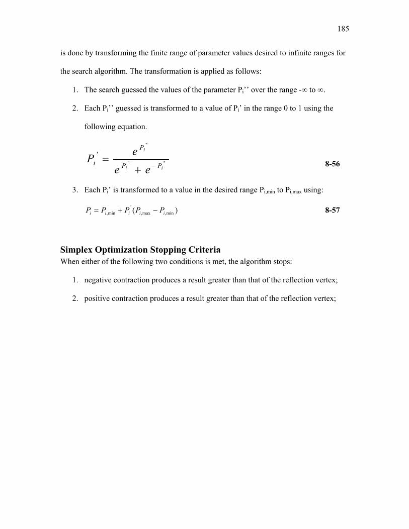
185
is done by transforming the finite range of parameter values desired to infinite ranges for
the search algorithm. The transformation is applied as follows:
1. The search guessed the values of the parameter Pi’’ over the range -∞ to ∞.
2. Each Pi’’ guessed is transformed to a value of Pi’ in the range 0 to 1 using the
following equation.
""
"
'
ii
i
PP
P
iee
eP−+
= 8-56
3. Each Pi’ is transformed to a value in the desired range Pi,min to Pi,max using:
)( min,max,'
min, iiiii PPPPP −+= 8-57
Simplex Optimization Stopping Criteria When either of the following two conditions is met, the algorithm stops:
1. negative contraction produces a result greater than that of the reflection vertex;
2. positive contraction produces a result greater than that of the reflection vertex;

186
Figure 8-6 Flow Chart of Modified Simplex Algorithm
Objective Function The objective function plays a crucial role in simplex method because it is used to
evaluate the performance of a set of values for all variables (a vertex). For an
optimization problem with only one response variable, the choice of objective function in
general is an easy problem. However in most practical optimization problems more than
one response variable must be considered at the same time [125]. There is no simple
solution to objection functions for multiple response variable problems because the

187
response variables are often in different scales, the significance of different response
variables differ, and the objectives for different response variable vary (i.e., some
response variables are to be maximized while others are to be minimized). In addition to
these difficulties, the description of optimization objectives is usually vague and
uncertain in the sense that the definitions of optimization objectives are not “black and
white”. For example, it is hard to say that a response of 100 is good but 99 is bad.
Despite the difficulties described above in determining objective functions, there are
some common methods of dealing with them. One common practice is the utilization of
fuzzy set theory with membership functions to form an optimization objective function
[125]. The approach is to form an aggregated joint response measure by combining
different response variables with different optimization objectives. The idea of
introducing fuzzy membership functions is to translate different response variables into a
measure that can be adequately compared and combined with others.
Other Considerations on the Utilization of Simplex Method Simplex methods are mostly used to optimize problems without constraints, that is, there
are no constraints on variables. However, this condition is often not true for real physical
problems. Thus, some measures are to be taken to deal with constraints. It is possible that
the simplex method converges to a non-optimal point even for simple problems [129]. It
was demonstrated by Barton et al. [130] that the choices of expansion and contraction
coefficients has an impact on the performance of simplex methods.

188
Appendix IV Modified MaxMin Thresholding The MaxMin thresholding method was developed by Torabi and is described in section
2.2.2.1. The threshold is the one giving the maximum minimum particle size as expressed
in Equation 8-58.
))((:1:0 ijnikj
AMinMaxT==
= 8-58
where T is the selected threshold value and Aij is the area of the ith particle visible in the
image using the jth value of threshold. For each jth value of threshold, the Minimum
particle size is found. The total number of threshold values examined, k, is set to 220 in
Torabi’s research.
The MaxMin thresholding was successful in determining the threshold value required to
separate the background from the particles in an image. However, here it was found to be
computationally very expensive: it required about 220 iterations (about 3 seconds) to
determine the threshold. This 3 second delay was about 90% of the total time required for
processing an image and was significant when hundreds of images were to be processed.
With the objective of reducing this delay time, in this research the following
modifications were made to the original Torabi Max Min method:
(a) Since, in this work, Image J provided a histogram of number of pixels versus grey
level it was possible to identify the actual minimum grey level in an image instead
of using zero as Torabi was obliged to. This reduced the range of possible “best”
grey level values.

189
(b) The highest “best” grey level of the image was taken to be the median grey value
of the image instead of the very high value of 220 specified by Torabi. It was
based upon the idea that the number of pixels belonging to particles accounts for
less than 5% percent of the total pixels of an image and the grey values of
particles are less than the average grey value of background which itself could be
represented by the median grey value of the image. The median grey value of an
image in most cases is below 220, which means that the maximum possible
“best” threshold value in Equation 8-58 will be below 220. Thus, like the first
modification, this change also narrowed the range of possible thresholds to
search.
(c) The step size for the threshold values used in the search was increased. The step
size is the interval between a preceding threshold value and the next value
examined. In Torabi’s work, the step size of the iteration was set to 1, i.e. the
search for the best threshold value examined every possible threshold values
between the starting threshold value (0 in Torabi’s work) and the ending
threshold value (220 in Torabi’s work). In this work, the step size is set to 5, i.e.,
if the starting threshold value is 100, the next threshold value to be examined is
105. Figure 8-7 shows an example image. The results of thresholding of it using
different step sizes are shown in Figure 8-8, which is a plot of minimum particle
size versus threshold. From the curve, the threshold giving the maximum
minimum particle size can be located. The peaks in the curves represent the
maximum minimum particle size in certain regions. As can be seen, different step
size will generate different curves. The curve for step size of 1 represents
190
thresholding results of all possible thresholds and accordingly it acts as
benchmark to verify if the use of other step sizes would be able to locate the true
peaks. It is observed that the application of other step sizes is unable to locate the
first peak though the second peak is located at step size of 5. However, what is
important is that the rough locations of major peaks are correctly identified by all
step sizes. This was very important because a further fine-resolution search could
be centered around the peaks to define the true peaks. In this work, it was
determined empirically that the step size of 5 should be sufficient to locate the
peaks.
The peak location-search using a larger step size provided the approximate location of
major peaks and ignored much smaller peaks. An assumption was made that the first two
peaks would be where the global threshold giving the maximum minimum particle size is
located. The assumption was well-founded in that:1) real particles tended to be darker,
have a low grey value and therefore they will turn out with a low threshold; 2) the use of
the first two peaks could avoid the situation that the first peak is noise, i.e., if the first
peak is noise, there is still the second peak. It is highly unlikely that both of the first two
peaks would be noise.

191
Figure 8-7 An Example Image
Minimum Particle Size Vs Threshold
0.00E+001.00E-052.00E-053.00E-054.00E-055.00E-056.00E-057.00E-058.00E-059.00E-051.00E-04
115 125 135 145 155 165
Threshold
Min
imum
Par
ticle
Siz
e
step size = 1 step size = 2 step size = 5 step size = 6
Figure 8-8 The Effect of Thresholding Step Size on Minimum Particle Size

192
Based on this assumption, a fine-resolution-search was carried out around a peak to
locate the local threshold which provided the maximum minimum particle size. The fine-
search method used in this work was the bisection algorithm. The modified search is
illustrated in Figure 8-9.
To describe how a modified novel search algorithm works, we use function min(x) to
represent the minimum particle size at threshold x. From Figure 8-9, we have
min(a)<min(b) and min(c)<min(b). With the assumption that the maximum minimum
particle size within [a,c] and provided that the curve between threshold a and c is convex,
the search will be performed as follows:
Step 1: Threshold the image using midpoint threshold (a+b)/2 and find min((a+b)/2).
Similarly find min((b+c)/2).
Step 2: Examine min((a+b)/2) and min((b+c)/2).
If min((a+b)/2) > min(b) and min(b) > min((b+c)/2), the maximum minimum particle
size (the true peak) must be within [a, b], so replace b with (a+b)/2 and replace c with b.
If min((b+c)/2) > min(b) and min(b) > min((a+b)/2), the peak must be within [b, c], and
therefore replace b with (b+c)/2 and replace a with b.
If min(b) > min((a+b)/2) and min(b) > min((b+c)/2), the peak must be within
[(a+b)/2,(b+c)/2], and therefore replace a with (a+b)/2 and replace c with (b+c)/2).
Step 3: If b-a =1 or c-b=1, b is the threshold giving the maximum minimum particle size
and search stops, otherwise return to the Step 1.

193
Minimum Particle Size vs Threshold
0.00E+001.00E-052.00E-053.00E-054.00E-055.00E-056.00E-057.00E-058.00E-059.00E-051.00E-04
110 120 130 140 150 160
Threshold
Min
imum
Par
ticle
Siz
e
a
b
c
(b+c)/2(a+b)/2
Figure 8-9 Scheme of Modified Search for Threshold
The Bisection search was performed on the first two peaks separately and there a
threshold for each peak giving a local maximum minimum particle size was identified.
The threshold specifying the maximum minimum particle size was accepted as the global
threshold.
The above modified MaxMin method was tested by applying it to 249 randomly selected
images. Results are tabulated in Table 8-3. There it can be seen that for 91.2% of the
images difference between the threshold selected by Modified MaxMin thresholding and
by the original MaxMin thresholding is less than or equal to 3. However, the modified
MaxMin thresholding greatly reduced the number of iterations required to search for the
global threshold with an average of 12 iterations compared to the original f 220,: this was
a reduction of 90%.

194
Table 8-3 Threshold Test of Modified MaxMin Thresholding Number of Images Percentage The threshold of bisection MaxMin thresholding is the same as that of original MaxMin Thresholding.
171 68.7%
The difference between the threshold of bisection MaxMin thresholding and that of original MaxMin Thresholding is within 3.
56 22.5%
The difference between the threshold of bisection MaxMin thresholding and that of original MaxMin Thresholding is more than 3.
22 8.8%
Thus, it appeared that there was very little difference in the threshold value selected by
the modified max min method and a large decrease in the umber of iterations required.
Next the effect on classification performance was examined.
A set of 745 images (240 WOs and 505 WPs) in off-line image modification as training
images were selected and thresholded using both MaxMin thresholding and Modified
MaxMin Thresholding. The classification results for the two thresholding methods are
tabulated in Table 8-4 and Table 8-5 respectively. As can be seen, there are 29 false
negatives and 49 false positives for MaxMin thresholding versus 16 and 25 for Modified
MaxMin thresholding, respectively. Thus, it was concluded that the Modified MaxMin
thresholding in fact improved the classification accuracy compared to the original
MaxMin thresholding. The classification error rates for the two methods are illustrated in
Figure 8-10, which shows that the error rates for Modified MaxMin thresholding reduced
in all aspects including over error rate, false negative rate and false positive rate as
compared to those of the original MaxMin thresholding. Modified MaxMin thresholding
has an overall error rate of 5.5% over 10.5% of the original MaxMin thresholding,
indicating a 5% improvement.
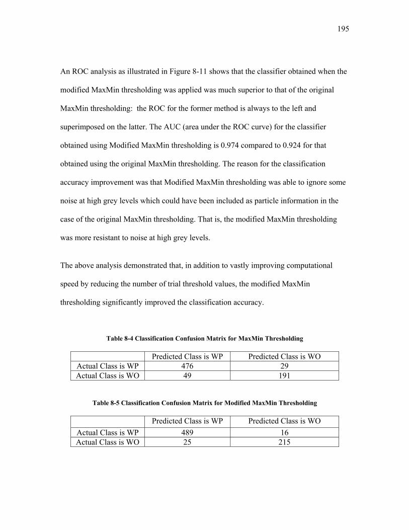
195
An ROC analysis as illustrated in Figure 8-11 shows that the classifier obtained when the
modified MaxMin thresholding was applied was much superior to that of the original
MaxMin thresholding: the ROC for the former method is always to the left and
superimposed on the latter. The AUC (area under the ROC curve) for the classifier
obtained using Modified MaxMin thresholding is 0.974 compared to 0.924 for that
obtained using the original MaxMin thresholding. The reason for the classification
accuracy improvement was that Modified MaxMin thresholding was able to ignore some
noise at high grey levels which could have been included as particle information in the
case of the original MaxMin thresholding. That is, the modified MaxMin thresholding
was more resistant to noise at high grey levels.
The above analysis demonstrated that, in addition to vastly improving computational
speed by reducing the number of trial threshold values, the modified MaxMin
thresholding significantly improved the classification accuracy.
Table 8-4 Classification Confusion Matrix for MaxMin Thresholding
Predicted Class is WP Predicted Class is WO Actual Class is WP 476 29 Actual Class is WO 49 191
Table 8-5 Classification Confusion Matrix for Modified MaxMin Thresholding
Predicted Class is WP Predicted Class is WO Actual Class is WP 489 16 Actual Class is WO 25 215
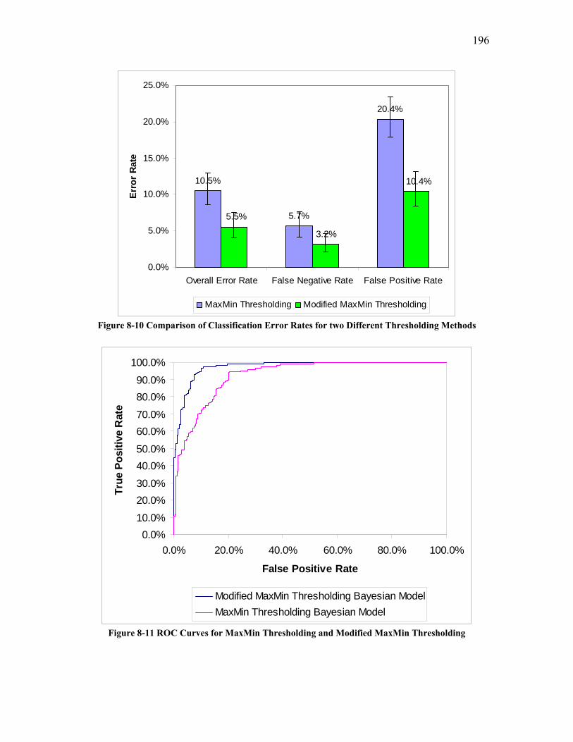
196
10.5%
5.7%
20.4%
10.4%
3.2%
5.5%
0.0%
5.0%
10.0%
15.0%
20.0%
25.0%
Overall Error Rate False Negative Rate False Positive Rate
Erro
r Ra
te
MaxMin Thresholding Modified MaxMin Thresholding
Figure 8-10 Comparison of Classification Error Rates for two Different Thresholding Methods
0.0%10.0%
20.0%30.0%
40.0%50.0%
60.0%70.0%
80.0%90.0%
100.0%
0.0% 20.0% 40.0% 60.0% 80.0% 100.0%
False Positive Rate
True
Pos
itive
Rat
e
Modified MaxMin Thresholding Bayesian ModelMaxMin Thresholding Bayesian Model
Figure 8-11 ROC Curves for MaxMin Thresholding and Modified MaxMin Thresholding
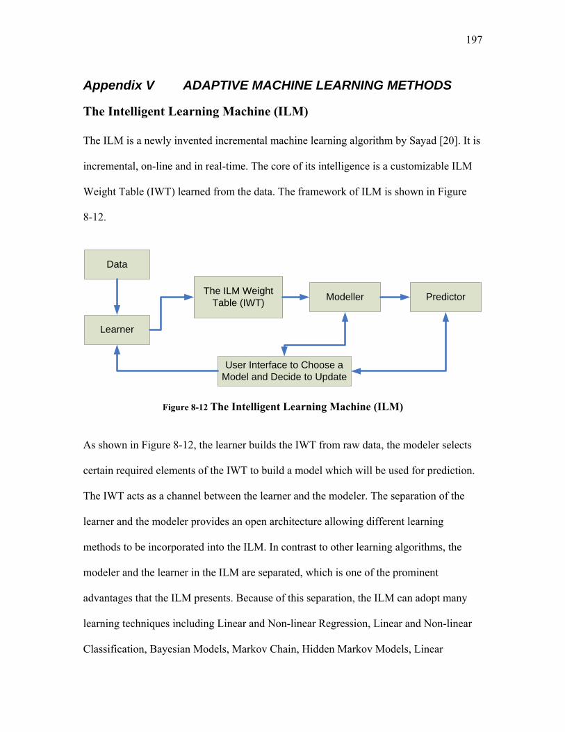
197
Appendix V ADAPTIVE MACHINE LEARNING METHODS
The Intelligent Learning Machine (ILM) The ILM is a newly invented incremental machine learning algorithm by Sayad [20]. It is
incremental, on-line and in real-time. The core of its intelligence is a customizable ILM
Weight Table (IWT) learned from the data. The framework of ILM is shown in Figure
8-12.
Data
Learner
PredictorModeller
User Interface to Choose a Model and Decide to Update
The ILM Weight Table (IWT)
Figure 8-12 The Intelligent Learning Machine (ILM) As shown in Figure 8-12, the learner builds the IWT from raw data, the modeler selects
certain required elements of the IWT to build a model which will be used for prediction.
The IWT acts as a channel between the learner and the modeler. The separation of the
learner and the modeler provides an open architecture allowing different learning
methods to be incorporated into the ILM. In contrast to other learning algorithms, the
modeler and the learner in the ILM are separated, which is one of the prominent
advantages that the ILM presents. Because of this separation, the ILM can adopt many
learning techniques including Linear and Non-linear Regression, Linear and Non-linear
Classification, Bayesian Models, Markov Chain, Hidden Markov Models, Linear

198
Discriminant Analysis, Association Rules, OneR rule, Principal Component Analysis,
and Linear Support Vector Machines. Furthermore, ILM is not limited to these
techniques.
The IWT, as the core of ILM, is a two dimensional table (Table 8-6). In this table, n is the
number of independent variables and m is the number of dependent variables. The basic
unit of ILM as shown in Table 8-7 is an independent variable Xj an dependent variable Xi,
and a weight Wi j. The Wi j contains four elements, namely, the number of data values, the
sum of variable Xj, the sum of variable Xi, and the sum of multiplication of variable Xi and
Xj, but other elements can be added to ILM if necessary.
Table 8-6 The General Structure of ILM Weight Table
X1 … Xj … Xn
X1 W11
…
W1 j
…
W1 n
… … … … … …
Xi
Wi1
…
Wi j
…
Wi n
… … … … … …
Xm
Wm1
…
Wm j
…
Wm n As shown in Table 8-7, the basic unit of the Knowledge Table includes a dependent
variable Xi , an independent variable Xj and a weight function Wij:
Table 8-7 The Basic Unit of the ILM Weight Table
Xi
Xj Nij ∑xi ∑xj ∑xij
199
Values of Xi and Xj are denoted xi and xj respectively. Wij consists of the following four
basic elements:
• Ni j is the total number of joint occurrences of xi and xj data values in the dataset
• Σ xi is the sum of values for variable Xi (i.e. xi) in the dataset with the summation over
Ni j the number of records containing the values.
• Σ xj is the sum of values for variable Xj in the dataset with the summation over Ni j the
number of records containing the values.
• Σ xi xj is the sum of multiplication of values for variables Xi and Xj in the dataset with
the summation over Ni j the number of records containing the values.
The structure of IWT allows the following actions to dynamically change the content of
IWT:
• learning, to add new data record into the IWT;
• forgetting, to remove data records from the IWT;
• growing, to add new variable into the IWT;
• contracting, to remove variables from the IWT;
• interacting, to extract certain part of the IWT for modeling;
• co-operating, to join other IWTs with the same structure.
These IWT actions provide the flexibility for various modeling needs.
The incremental, online and real-time characteristics of ILM dramatically reduce the
computation load in terms of adding new data records to the model, removing data
records and modeling change with the addition or removal of variables. In addition, the
co-operation feature of IWT allows parallel and distributed processing of large and

200
complex datasets. This feature along with the incremental learning nature presents ILM
with full potential for real-time process monitoring and pattern recognition.
Application of ILM to Naïve Bayesian Model for Image Classification In this work the Bayesian model was used to estimate the probability that an image is
With Particle (WP) or Without Particle (WO). The estimated probability was calculated
based on two attributes of an image, i.e., “mean grey value” and “percentage area”. These
attributes are the “Xi” in the Knowledge Table as in Table 8-6. The decision whether an
image is WO or WP is thus determined by the two estimated probabilities to be the class
giving the higher probability. Please refer to chapter 2 for details of calculating
probability.
For a Naïve Bayesian model, only the diagonal cells as in Table 8-6 are needed to
estimate the desired WP or WO probability since the other cells representing interaction
between attributes are not concerned and ignored. In this research, to applying the ILM
to the Naïve Bayesian classification model, two Knowledge tables (IWT) are needed, one
for calculating the probability of WP and the other for calculating the WO probability.
The WP table contains data of image known to be WP and WO table for images known
to be WO.
Table 8-8 shows a Knowledge Table in this work. It is noted that only diagonal cells are
present. N1 and N2 are the number of occurrences of each attribute. In this work, since
there is no missing value of attribute for all the images. N1 and N2 are, in fact, the
number of images (N) used to create the IWT. In the cases where there are missing

201
attribute values, Ni could be different for different cells of the Knowledge Table and
would need to be calculated accordingly.
Table 8-8 ILM Knowledge Table for N images
X1 X2
X1 N1 Σx1 Σx1
2
X2
N2 Σx2 Σx2
2
The calculation of mean and standard deviation of an attribute (using the first attribute
as an example) is given in Equation 8-59 and 8-61.
21 NNN == 8-59 (1)
8-60
8-61 In the above equations, subscript 1 is designated to be the indicator of first attribute and
subscript i is designated to be the ith images.
One of the major advantages of the ILM is its efficient incremental learning capability.
Thanks to the assumption of attribute independence, Naïve Bayesian model is
intrinsically incremental. However, practically taking advantage of this property
efficiently is not as apparent as it seems. The ILM enables an extremely efficient and
systematic way of merging new data into a Bayesian model by aggregating historical data
N
xN
ii∑
== 11μ
21
11
21
1
211
21
)()(
N
x
N
x
N
xN
ii
N
ii
N
ii ∑∑∑
=== −=−
=μ
σ
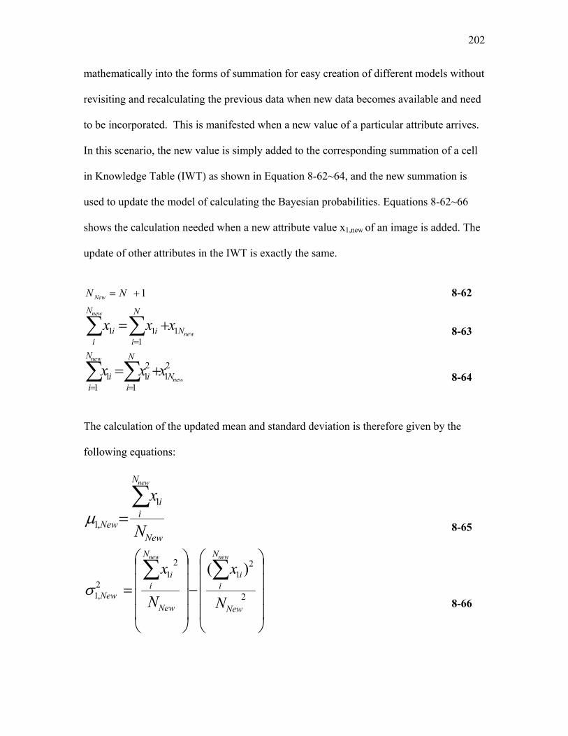
202
mathematically into the forms of summation for easy creation of different models without
revisiting and recalculating the previous data when new data becomes available and need
to be incorporated. This is manifested when a new value of a particular attribute arrives.
In this scenario, the new value is simply added to the corresponding summation of a cell
in Knowledge Table (IWT) as shown in Equation 8-62~64, and the new summation is
used to update the model of calculating the Bayesian probabilities. Equations 8-62~66
shows the calculation needed when a new attribute value x1,new of an image is added. The
update of other attributes in the IWT is exactly the same.
1+= NN New 8-62
new
new
N
N
ii
N
ii xxx 1
111 ∑∑
=
+= 8-63
21
1
21
11 new
new
N
N
ii
N
ii xxx ∑∑
==
+= 8-64
The calculation of the updated mean and standard deviation is therefore given by the
following equations:
New
N
ii
New N
xnew
∑=
1
,1μ 8-65
⎟⎟⎟⎟
⎠
⎞
⎜⎜⎜⎜
⎝
⎛
−⎟⎟⎟⎟
⎠
⎞
⎜⎜⎜⎜
⎝
⎛
=∑∑
2
21
21
2,1
)(
New
N
ii
New
N
ii
New N
x
N
xnewnew
σ 8-66

203
As can be seen, the calculations involved in incremental learning using the ILM is at a
minimum level compared to other popular incremental methods. This property is very
suited to a real-time system because it saves significant computation time. This is often
very critical for a system which needs to be very responsive system in an environment
where large amount of are generated at a very high speed.
Incremental Support Vector Machine (ISVM) While the Support Vector Machine (SVM) has been widely studied, the study of ISVM
began just a few years ago [22, 131-138]. One of the known issues with the SVM is high
computation complexity since training a SVM requires solving a quadratic programming
(QP) problem with a number of coefficients equal to the number of training examples
[134]. QP is computationally intensive, takes a long time to converge and requires
memory. Thus for a large dataset, especially in real-time, standard numeric techniques for
QP are infeasible and generate a scalability issue for SVM. When adding new data
records to a large training set, an efficient ISVM becomes necessary to avoid batch
retraining.
An early study of ISVM by Syed [131] suggested retraining a classifier with all support
vectors (SV) and newly added samples. The reasoning behind this is as follows: the
resulting decision function of an SVM depends only on its SVs, i.e. training an SVM on
the SVs alone results in the same decision function as training on the whole data set.
Therefore one expects to obtain an incremental result that is equal to the non-incremental
result, if the last training set contains all SVs in the non-incremental case. The empirical
204
results from this research show that ISVM performs well even though this training
scheme provides approximate results.
Xiao [133] presented a similar technique for incremental training of the SVM. In his
research, all training samples are divided into three sets, a backup set (mostly of trivial
samples), a caching set (samples frequently appearing in SV set) and a work set (the
latest SV set). With the definition of these three types of samples, a Least-Recently Used
(LRU) scheme is implemented to optimally discard trivial samples without sacrificing the
classification precision.
Both ISVM methods mentioned above are approximate approaches. An exact incremental
learning of SVM was proposed by Cauwenberghs et al. [134]. In their method, the exact
solution is constructed recursively by adding one new data point at a time while retaining
the Kuhn-Tucher conditions on all previous data. Experiment with an example data set
shows that incremental learning offer a simple and computationally efficient scheme. The
procedure can be extended to SV regression.
Peng et al. [137] proposed an active learning scheme. The scheme first interrogates the
new data point by measuring the distance between the point and the hyper-plane
consisting of the entire SV set. A threshold is then applied to the measured distances. If
the distance is smaller than the threshold, the new data point will be added to the current
SV set as new training set. Otherwise the new data point is discarded. This strategy does
achieve computational efficiency but the choice of threshold is empirical. This method in
some sense is desirable for real-time process monitoring in which data is generated very
fast.
205
An et al. [22] presented an even more aggressive incremental learning method by pre-
extracting the SV set for initial training and post-discarding training samples in an
attempt to lower the training load. The initial training phase consists of three steps. In the
first step, the pre-extracting SV set is selected based on the least distance between the
samples in two classes and this is used as a work set to obtain the classifier. Next, the
obtained classifier is applied to classify samples which are not in the training set. Those
samples whose relative distances to the SV hyper-plane are greater than a threshold will
be added to the work set while others will become training samples for the next iteration.
Finally, the process iterates to the first step until all training samples are correctly
classified. In the incremental training phase, the new data points are classified using the
current SV set as the second step in the initial training phase. The rest of the incremental
training is the same as the initial training. After the iteration terminates, some training
samples are discarded following the similar scheme proposed by Peng [137]. However,
Peng’s scheme was to discard the newly added training samples.
Although ISVM attracts much attention and has great potential, further studies are
required. ISVM so far has not been implemented in real-world applications. In
comparison, ILM has an advantage over ISVM for linear problems because once the IWT
in ILM is constructed, there is no need to work with the original raw data.
Incremental Neural Networks (INN) Artificial neural networks (ANN) have been widely used in image processing and
analysis, process control and chemistry as they are universal function approximators for
206
linear, non-linear and even unknown relationships. In this literature review, however, the
attention will be given to incremental neural networks (INN) which is more desirable for
real-time supervised or supervised clustering and classification applications. Among
INNs, fuzzy adaptive resonance theory (ART) and Fuzzy ARTMAP are emphasized.
Like other non-incremental learning algorithms, backpropagation based neural networks
encountered the problem that a classifier trained on a data set often suffers: unacceptable
classification accuracies on a new data set. From an operational point of view, such a
problem represents a serious limitation in real-world applications (e.g., automatic image
monitoring systems, robot learning) in which data sets tend to vary significantly. In this
context, the design of a robust incremental learning system capable of performing
efficiently and improving its generalization on different data sets is very desirable. Only
a few papers [24, 28, 31, 139-144] have been published that deal with the incremental-
learning NN, so it is still an open issue in the pattern-recognition literature.
The first true incremental neural network is proposed by Park et al. [31]. In his research,
a training procedure that adapts the weights of a trained layered perceptron artificial
neural network to training data originating from a slowly varying non-stationary process
is proposed. The resulting adaptively trained neural network, based on a nonlinear
programming techniques, is shown to adapt to new training data that are in conflict with
earlier training data without affecting the neural networks' response to data elsewhere. Fu
et al. [28] proposed an incremental backpropagation learning neural network (IBPLN) for
classification based on bounded weight adaptation and structural adaptation learning
rules. The main idea is to add a hidden unit (i.e., change the topology of the network). If

207
the neural network cannot accommodate the new instance through weight adaptation, and
this process is called neuron generation. A previously added hidden unit was deleted if its
output weight decayed to a predefined threshold value. This is called neuron elimination.
However, one of the drawbacks of IBPLN is that it can not adapt to a new data set
containing new classes. A constructive, incremental learning system for regression
problems is introduced by Schaal [141].
Bruzzone et al. [24] proposes an incremental Radial Basis Function (RBF) based neural
network for the classification of remote-sensing images. The proposed classifier, a three-
layered network, allows adaptation to new classes possibly contained in the new data
sets. The initial training phase follows the same two-step procedure as training a normal
RBF neural network. That is, it first obtains the prototypes by applying a clustering
procedure to the training samples of each class, and then calculates the weight matrix by
minimizing the sum-of-squares error function. In the incremental training phase, a
similarity function between a new sample and its closest existing prototype is defined. If
a sample is found to be similar to its closest prototype, then the prototype is updated;
otherwise, a new prototype is generated because the new sample considered cannot be
efficiently represented by any current existing prototypes. The generation of a new
prototype means the addition of new neuron with a new kernel function. Following the
prototype updating, the weight updating is performed again based on the error function.
This classifier is capable of performing incremental learning and approximately
preserving the ‘old’ knowledge in the incremental learning phase. Furthermore, it
exhibits the characteristics of self-organization and network topology adaptability.

208
Appendix VI Screen 3: Selection of IQ Operators by Task Specific Criteria
In Screen 3 an experimental design is used to generate images utilizing the IQ Operators
obtained from the Screen 2 selection. The objective of the experimental design is to
assess important “task specific criteria”. Task specific considerations included the effect
of an IQ Operator on task specific image quality characteristics and the task specific
computational characteristics of an IQ Operator. The latter term refers to the fact that for
in-line monitoring, calculation speed and simplicity are important characteristics.
In Screen 3 these considerations led to two criteria being used to select the most desirable
IQ Operators:
i. the effect on particle image size;
ii. the absence of interaction effects on particle image size with other IQ Operators.
IQ Operators (as shown in Table 8-9) with the low and high levels of their parameters
according to Table 5-1 were applied to various test patterns in combinations as dictated
by the statistical experimental design. Statistical experimental design analysis software
was developed and interfaced with the commercially available Image J program so that
the design could be implemented on images. In developing Screen 3, four trials were
conducted using test patterns as images and are summarized in Table 8-9. “Order of
Application” was a blocking variable. That is, each design was limited to one order of
application.
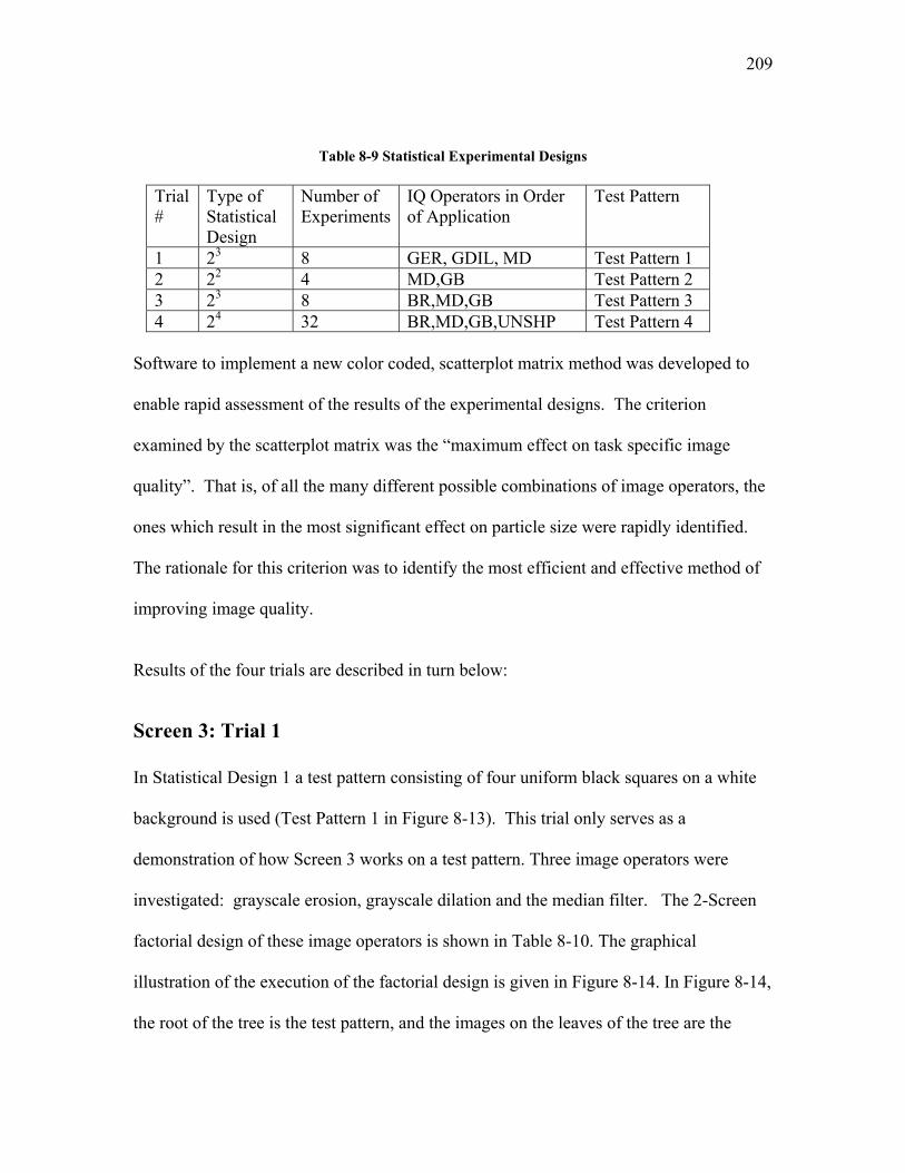
209
Table 8-9 Statistical Experimental Designs
Trial #
Type of Statistical Design
Number of Experiments
IQ Operators in Order of Application
Test Pattern
1 23 8 GER, GDIL, MD Test Pattern 1 2 22 4 MD,GB Test Pattern 2 3 23 8 BR,MD,GB Test Pattern 3 4 24 32 BR,MD,GB,UNSHP Test Pattern 4
Software to implement a new color coded, scatterplot matrix method was developed to
enable rapid assessment of the results of the experimental designs. The criterion
examined by the scatterplot matrix was the “maximum effect on task specific image
quality”. That is, of all the many different possible combinations of image operators, the
ones which result in the most significant effect on particle size were rapidly identified.
The rationale for this criterion was to identify the most efficient and effective method of
improving image quality.
Results of the four trials are described in turn below:
Screen 3: Trial 1 In Statistical Design 1 a test pattern consisting of four uniform black squares on a white
background is used (Test Pattern 1 in Figure 8-13). This trial only serves as a
demonstration of how Screen 3 works on a test pattern. Three image operators were
investigated: grayscale erosion, grayscale dilation and the median filter. The 2-Screen
factorial design of these image operators is shown in Table 8-10. The graphical
illustration of the execution of the factorial design is given in Figure 8-14. In Figure 8-14,
the root of the tree is the test pattern, and the images on the leaves of the tree are the
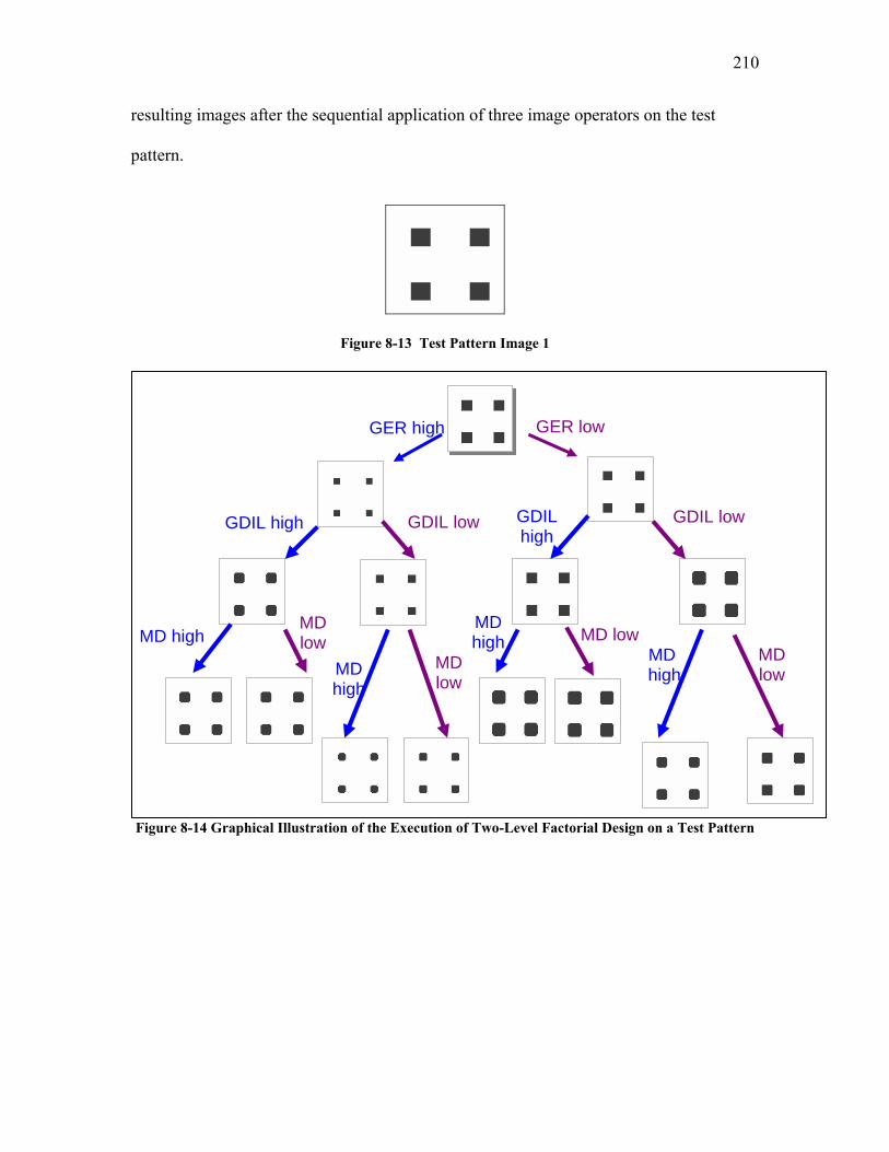
210
resulting images after the sequential application of three image operators on the test
pattern.
Figure 8-13 Test Pattern Image 1
Figure 8-14 Graphical Illustration of the Execution of Two-Level Factorial Design on a Test Pattern
MD high MD high MD low
GDIL high
MD high
GER lowGER high
GDIL lowGDIL lowGDIL high
MD low
MD low
MD low
MD high
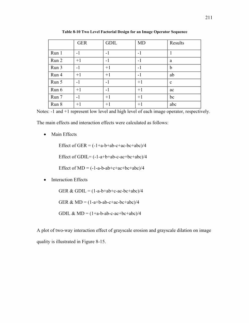
211
Table 8-10 Two Level Factorial Design for an Image Operator Sequence
GER GDIL MD Results
Run 1 -1 -1 -1 1 Run 2 +1 -1 -1 a Run 3 -1 +1 -1 b Run 4 +1 +1 -1 ab Run 5 -1 -1 +1 c Run 6 +1 -1 +1 ac Run 7 -1 +1 +1 bc Run 8 +1 +1 +1 abc
Notes: -1 and +1 represent low level and high level of each image operator, respectively.
The main effects and interaction effects were calculated as follows:
• Main Effects
Effect of GER = (-1+a-b+ab-c+ac-bc+abc)/4
Effect of GDIL= (-1-a+b+ab-c-ac+bc+abc)/4
Effect of MD = (-1-a-b-ab+c+ac+bc+abc)/4
• Interaction Effects
GER & GDIL = (1-a-b+ab+c-ac-bc+abc)/4
GER & MD = (1-a+b-ab-c+ac-bc+abc)/4
GDIL & MD = (1+a-b-ab-c-ac+bc+abc)/4
A plot of two-way interaction effect of grayscale erosion and grayscale dilation on image
quality is illustrated in Figure 8-15.

212
Figure 8-15 Plot of Two-Way Interaction Effect of Grayscale Erosion and Grayscale Dilation In Figure 8-16, the vertical axis represents the image quality, and the horizontal axis
represents the image operator erosion at two levels, and the two lines shows the change in
image quality at high and low level of image operator dilation. The plot indicates the
trends of main effects and interaction effects of image operators on the image quality.
More specifically, the plot shows that particle size decreases as operator erosion level
goes from low to high. While for operator dilation, it is opposite. The two slightly
converging lines indicate that there is a weak interaction effect between image operators
erosion and dilation.
The classical scatter plot is limited to a pair of variables. Thus, when more than two
variables are involved many such plots are required to include all the possible two way
combinations. The plots can be arranged as a matrix to form a “scatterplot matrix”. This
has been done in the literature for multiple two way scatterplots but its application to the
“interaction” plots from a statistical experimental design has not previously been
published. To assess the effects of image operators on image quality using a scatterplot
matrix, it is desirable to highlight the effects by color coding each cell of the matrix
Dilation Low
Dilation High
0
50
100
150
200
250
300
350
400
0 0.5 1 1.5 2 2.5 3 3.5
Erosion
Par
ticle
Siz
e (in
pix
els)

213
according to the magnitude of the effects it shows as shown in Figure 8-16. Diagonal cell
shows the main effect of an independent variable on the response variable and the off-
diagonal cells shows the interaction effect of two independent variables on the response
variable. In this way, we are able to visually identify the major variables which have the
strongest contribution to image quality rapidly and easily. Figure 8-16 shows a newly
designed color-coded scatterplot matrix for a sequence of three operator operations. Each
scatter plot in the matrix represents one response variable and one or two independent
variables. In this case, the response variable is the image quality metric (particle size),
and the two independent variables are two IQ Operators. The horizontal axis of a scatter
plot is the IQ Operator indicated by the title of the column where the particular scatter
plot is located, and the other image operator is indicated inside that scatter plot. The
effects of image operators on image quality are color coded in the scatter plots only if the
magnitudes of the effects are above a predefined threshold. In this case, the threshold is
set to five percent of the original image quality (particle size). For the diagonal scatter
plots in the matrix, the coded colors are for main effects, while for the rest of scatter
plots, the coded colors are for interaction effect. The color is assigned to each scatter plot
according to the color bar by the right side of the matrix. Figure 8-16 shows that
grayscale erosion has a strong main effect on image quality, while grayscale dilation has
a relative weak main effect. The two-way interaction effect between grayscale erosion
and grayscale dilation exceeds five percent but it is less significant in comparison with
the main effects of grayscale erosion and grayscale dilation. All other effects are
negligible with magnitude less than five percent. With the criterion of selecting the
operators with the strongest effects on image quality, grayscale erosion and grayscale

214
dilation are selected in this case because they are the ones which most effectively and
efficiently change the image quality.
Figure 8-16 Color-coded Scatterplot Matrix for Sequence of Grayscale dilation, Grayscale erosion
and Median filter
Screen 3: Trial 2 In Trial 2 a test pattern consisting of four uniform black squares on a white background
with impulsive and white noise is used (Test Pattern 2 in Figure 8-17). Two image
operators were investigated: median filter and Gaussian Blur filter. The median filter
was chosen because there are impulsive noises in the Test Pattern 2, and the Gaussian
filter was selected due to the presence of white noise. The 2-Level factorial design of

215
these image operators is similar to that in statistical design 1. The color-coded scatterplot
matrix for the image process sequence meeting the two selection criterions mentioned
above is shown in Figure 8-18. In this case, only media filter is chosen while Gaussian
Blur is eliminated because its main effect is below the threshold of five percent
predetermined.
Figure 8-17 Test Pattern Image 2
Figure 8-18 Color-coded Scatterplot Matrix for Sequence of Median and Gaussian Filters
Screen 3: Trial 3 In Trial 3 a test pattern consisting of four uniform black squares on a white background
with impulsive and white noise is used (Test Pattern 3 in Figure 8-19). Three image
operators were investigated: brightness shift, median filter and Gaussian filter. The
selection of brightness shift is based on the fact that both image background and
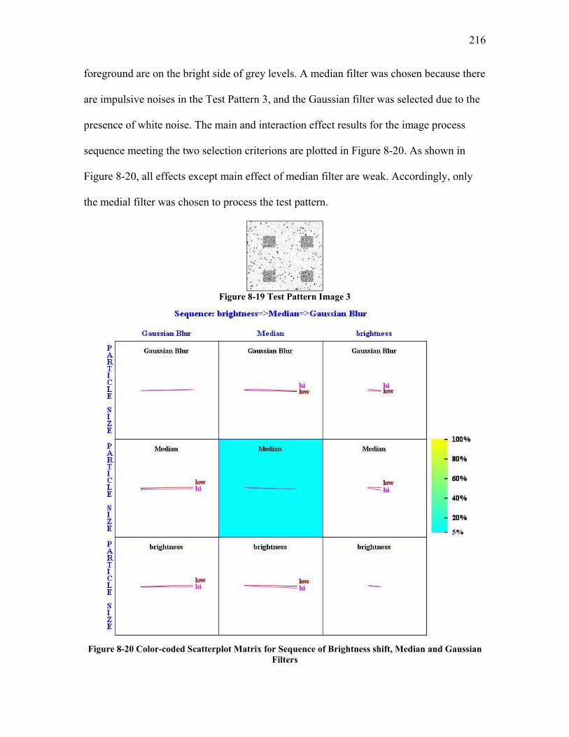
216
foreground are on the bright side of grey levels. A median filter was chosen because there
are impulsive noises in the Test Pattern 3, and the Gaussian filter was selected due to the
presence of white noise. The main and interaction effect results for the image process
sequence meeting the two selection criterions are plotted in Figure 8-20. As shown in
Figure 8-20, all effects except main effect of median filter are weak. Accordingly, only
the medial filter was chosen to process the test pattern.
Figure 8-19 Test Pattern Image 3
Figure 8-20 Color-coded Scatterplot Matrix for Sequence of Brightness shift, Median and Gaussian
Filters
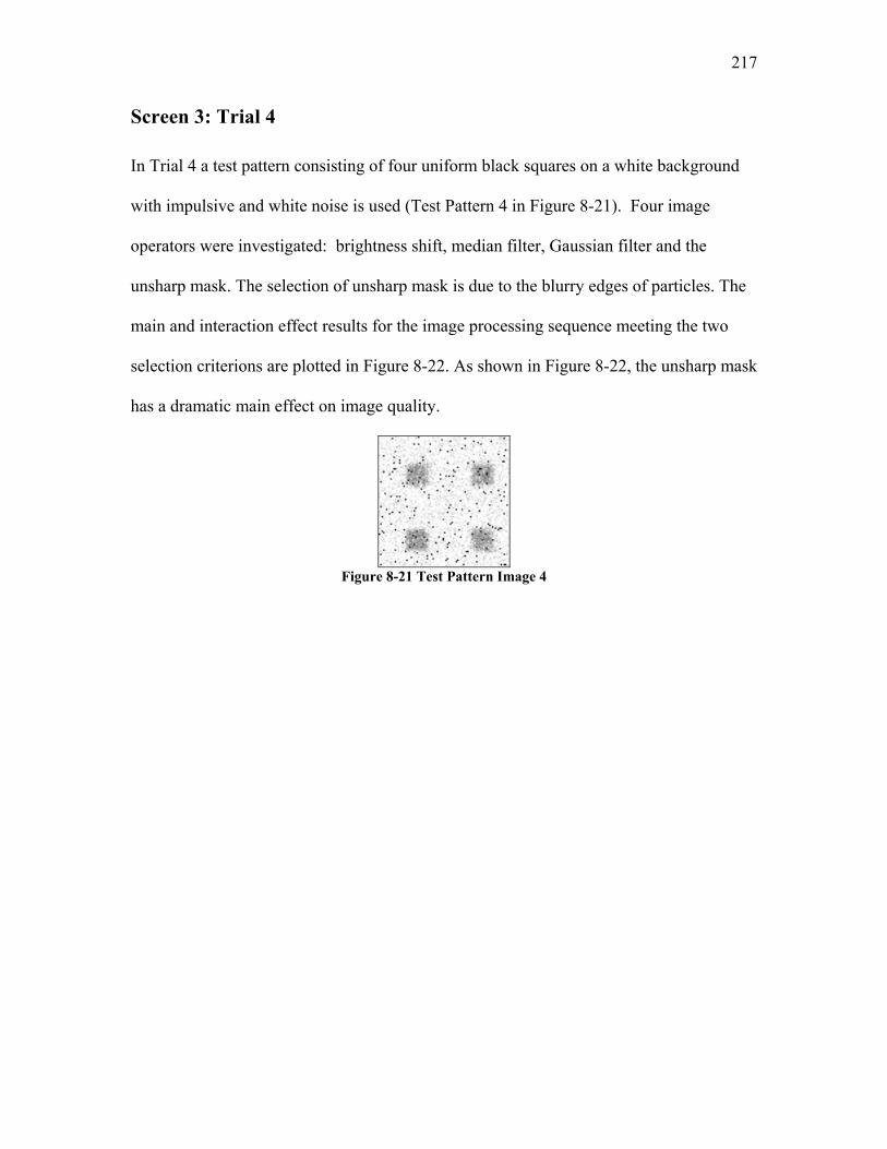
217
Screen 3: Trial 4
In Trial 4 a test pattern consisting of four uniform black squares on a white background
with impulsive and white noise is used (Test Pattern 4 in Figure 8-21). Four image
operators were investigated: brightness shift, median filter, Gaussian filter and the
unsharp mask. The selection of unsharp mask is due to the blurry edges of particles. The
main and interaction effect results for the image processing sequence meeting the two
selection criterions are plotted in Figure 8-22. As shown in Figure 8-22, the unsharp mask
has a dramatic main effect on image quality.
Figure 8-21 Test Pattern Image 4
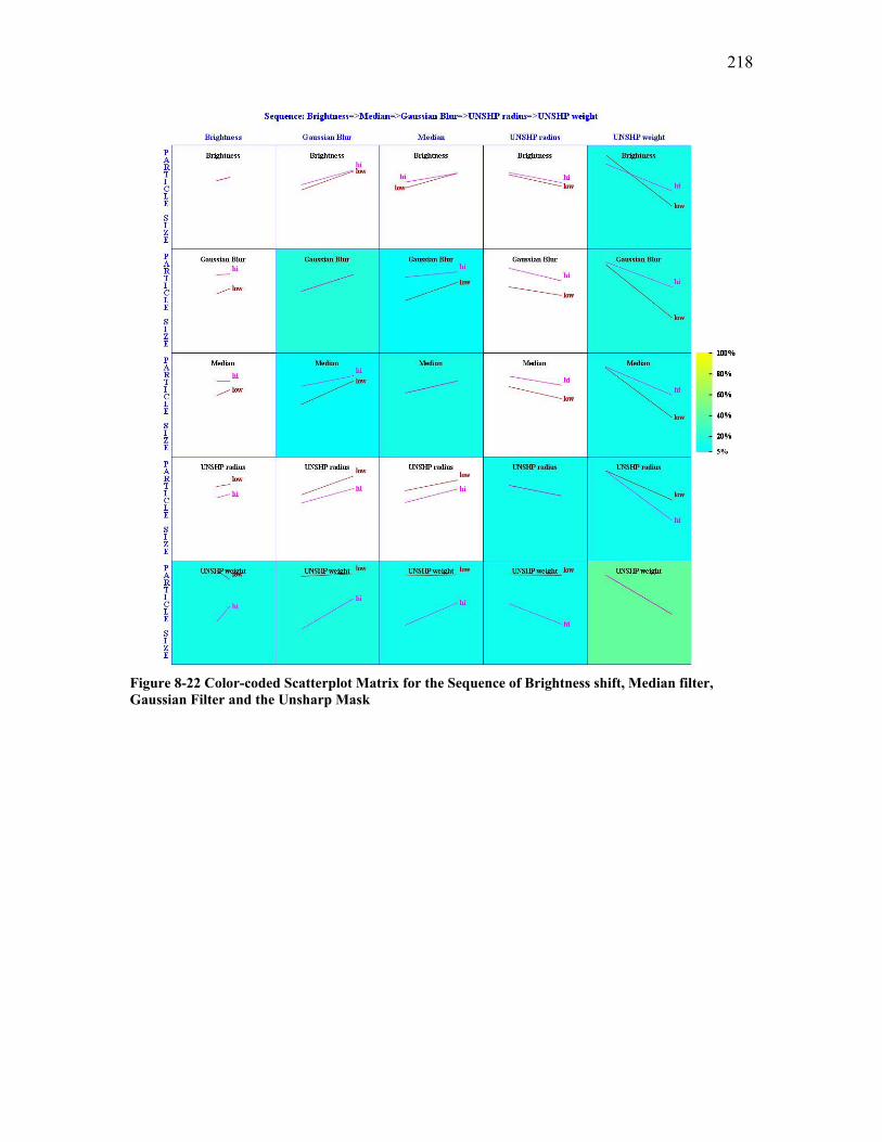
218
Figure 8-22 Color-coded Scatterplot Matrix for the Sequence of Brightness shift, Median filter, Gaussian Filter and the Unsharp Mask
219
Appendix VII Case-Based Reasoning Classification
This appendix summarizes the results of an investigation into the possibility of using
Case-Based Reasoning Classification (termed CBR Classification) instead of Bayesian
Classification to assign a new image a WP or WO class label. The CBR Classification is
illustrated in Figure 8-23. With CBR Classification, the same attributes and similarity
measurement as in Table 5-18 were applied to retrieve the most similar image case in the
database. However, then the class label of this image case was retrieved and assigned to
be the class of the new testing image: image processing instructions were not used since
no image quality improvement was involved. This is the simplest way to employ CBR
Classification. Hybrid methods involving both image quality improvement and CBR
Classification could be envisioned but were not examined in this supplemental
investigation.
Figure 8-24 shows the software component developed to implement CBR Classification.
As illustrated, first a blanket image processing step including brightness adjustment and
background flattening was applied to the new input testing image. Next, the image
quality metrics and necessary attributes of particles of the new image were measured by
invoking the image measurement shared software component. The measurements were
then used by the database shared software component to locate the most similar image
case in the Reference Image Database to the new image. The class label associated with
the retrieved image case was then assigned to the new image.
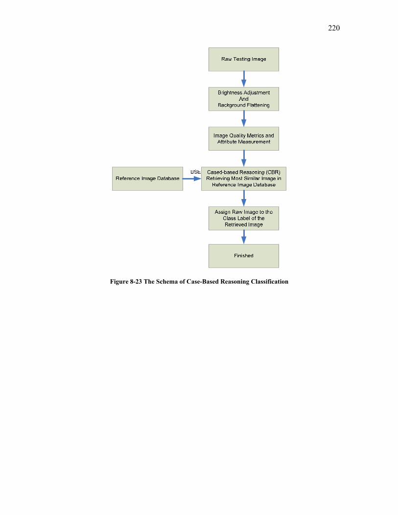
220
Figure 8-23 The Schema of Case-Based Reasoning Classification

221
Locate Reference Image Closely Resembling the
Input Image
Assign to the Raw Image the Class Label of the Retrieved Image in the
Reference Image Database
Case-Based Reasoning
Classification
Measurement of Image Quality Metrics and Other
Attributes
Input Testing Image
Image MeasurementShared Component
DatabaseShared Component
Brightness AdjustmentAnd
Background Flattening
Image ProcessingShared Component
Figure 8-24 The Case-Based Reasoning Classification Component
The results of CBR Classification were obtained for the four trial image sets described in
Section 5.2.3 and compared with those of Torabi Adaptive Classification, Static IQMod
Classification and Adaptive IQMod Classification method.
Test Trial 1: the Use of a New Set of Images Produced by Torabi For this trial image set, the classification results of CBR Classification are shown in
Table 8-11.
Table 8-11 Confusion Matrix of Test Trial 1 Image Set Using CBR Classification
Predicted Class is WP Predicted Class is WO Actual Class is WP 234 2 Actual Class is WO 3 422

222
1.4%
14.8%
9.4%
0.7%0.8%0.8%
3.8%
0.5%1.7%
0.6% 0.7%0.4%
0.0%
2.0%
4.0%
6.0%
8.0%
10.0%
12.0%
14.0%
16.0%
18.0%
Overall Error Rate False Negative Rate False Positive Rate
Perc
enta
ge
In-line Adaptive Classification CBR ClassificationIQMod Classification Adaptive IQMod Classification
Figure 8-25 Comparison of Classification Error Rates for Test Trial 1 Using Different Classification
Methods Figure 8-25 showed that CBR Classification performed reasonably well for this trial
image set with an overall error rate of 0.8%. This is slightly higher than the 0.6% by
Adaptive IQMod Classification. The ability of the CBR Classification to adapt to image
quality variability was not examined.
Test Trial 2: the Use of the Microgel Image Set Produced by Ing For the Trial 2 image set, the classification results of CBR Classification are shown in
Table 8-12.
Table 8-12 Confusion Matrix of Test Trial 2 Image Set Using CBR Classification
Predicted Class is WP Predicted Class is WO Actual Class is WP 87 1 Actual Class is WO 0 1256
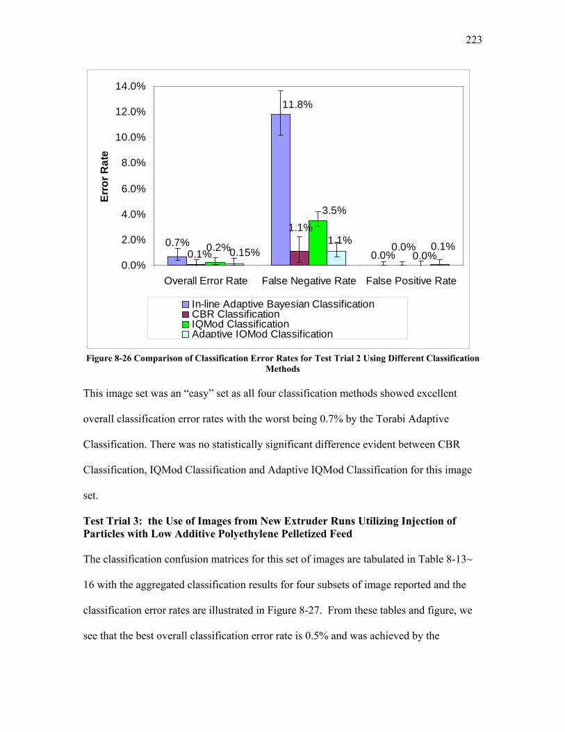
223
0.0%
11.8%
0.7% 0.0%
1.1%
0.1%0.2%
3.5%
0.0%0.1%1.1%
0.15%0.0%
2.0%
4.0%
6.0%
8.0%
10.0%
12.0%
14.0%
Overall Error Rate False Negative Rate False Positive Rate
Erro
r Rat
e
In-line Adaptive Bayesian ClassificationCBR ClassificationIQMod ClassificationAdaptive IQMod Classification
Figure 8-26 Comparison of Classification Error Rates for Test Trial 2 Using Different Classification
Methods This image set was an “easy” set as all four classification methods showed excellent
overall classification error rates with the worst being 0.7% by the Torabi Adaptive
Classification. There was no statistically significant difference evident between CBR
Classification, IQMod Classification and Adaptive IQMod Classification for this image
set.
Test Trial 3: the Use of Images from New Extruder Runs Utilizing Injection of Particles with Low Additive Polyethylene Pelletized Feed The classification confusion matrices for this set of images are tabulated in Table 8-13~
16 with the aggregated classification results for four subsets of image reported and the
classification error rates are illustrated in Figure 8-27. From these tables and figure, we
see that the best overall classification error rate is 0.5% and was achieved by the

224
Adaptive IQMod Classification method. This was followed by an error rate of 8.6% from
the Static IQMod Classification method. The CBR Classification method with an error
rate of 17.9% was significantly higher than the Adaptive IQMod and Static IQMod
Classification methods but significantly lower than the Torabi Adaptive method. Not
unexpectedly, CBR Classification was far less tolerant of image quality changes than
either Adaptive IQMod or Static IQMod as it didn’t involve any image quality
improvement process.
Table 8-13 Confusion Matrix for Test Trial 3 Image Subset (Run 3-1 to Run 3-4 in Table 3-2) Using Torabi Adaptive Classification
Predicted Class is WP Predicted Class is WO
Actual Class is WP 423 686 Actual Class is WO 0 363
Table 8-14 Confusion Matrix for Test Trial 3 Image Subset (Run 3-1 to Run 3-4 in Table 3-2) Using CBR Classification
Predicted Class is WP Predicted Class is WO
Actual Class is WP 845 264 Actual Class is WO 0 363
Table 8-15 Confusion Matrix for Test Trial 3 Image Subset (Run 3-1 to Run 3-4 in Table 3-2) Using
Static IQMod Classification
Predicted Class is WP Predicted Class is WO Actual Class is WP 982 127 Actual Class is WO 2 361
Table 8-16 Confusion Matrix for Test Trial 3 Image Subset (Run 3-1 to Run 3-4 in Table 3-2) Using
Adaptive IQMod Classification
Predicted Class is WP Predicted Class is WO Actual Class is WP 1101 8 Actual Class is WO 5 358
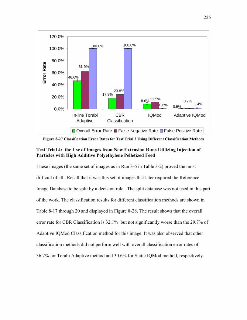
225
0.5%8.6%
46.6%
17.9%23.8%
11.5%
61.9%
0.7%1.4%
100.0%
0.6%
100.0%
0.0%
20.0%
40.0%
60.0%
80.0%
100.0%
120.0%
In-line TorabiAdaptive
CBRClassification
IQMod Adaptive IQMod
Erro
r R
ate
Overall Error Rate False Negative Rate False Positive Rate
Figure 8-27 Classification Error Rates for Test Trial 3 Using Different Classification Methods Test Trial 4: the Use of Images from New Extrusion Runs Utilizing Injection of Particles with High Additive Polyethylene Pelletized Feed These images (the same set of images as in Run 3-6 in Table 3-2) proved the most
difficult of all. Recall that it was this set of images that later required the Reference
Image Database to be split by a decision rule. The split database was not used in this part
of the work. The classification results for different classification methods are shown in
Table 8-17 through 20 and displayed in Figure 8-28. The result shows that the overall
error rate for CBR Classification is 32.1% but not significantly worse than the 29.7% of
Adaptive IQMod Classification method for this image. It was also observed that other
classification methods did not perform well with overall classification error rates of
36.7% for Torabi Adaptive method and 30.6% for Static IQMod method, respectively.
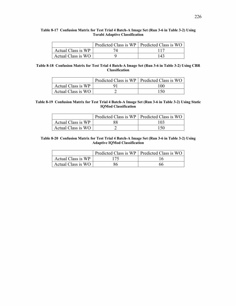
226
Table 8-17 Confusion Matrix for Test Trial 4 Batch-A Image Set (Run 3-6 in Table 3-2) Using Torabi Adaptive Classification
Predicted Class is WP Predicted Class is WO
Actual Class is WP 74 117 Actual Class is WO 9 143
Table 8-18 Confusion Matrix for Test Trial 4 Batch-A Image Set (Run 3-6 in Table 3-2) Using CBR
Classification
Predicted Class is WP Predicted Class is WO Actual Class is WP 91 100 Actual Class is WO 2 150
Table 8-19 Confusion Matrix for Test Trial 4 Batch-A Image Set (Run 3-6 in Table 3-2) Using Static
IQMod Classification
Predicted Class is WP Predicted Class is WO Actual Class is WP 88 103 Actual Class is WO 2 150
Table 8-20 Confusion Matrix for Test Trial 4 Batch-A Image Set (Run 3-6 in Table 3-2) Using
Adaptive IQMod Classification
Predicted Class is WP Predicted Class is WO Actual Class is WP 175 16 Actual Class is WO 86 66
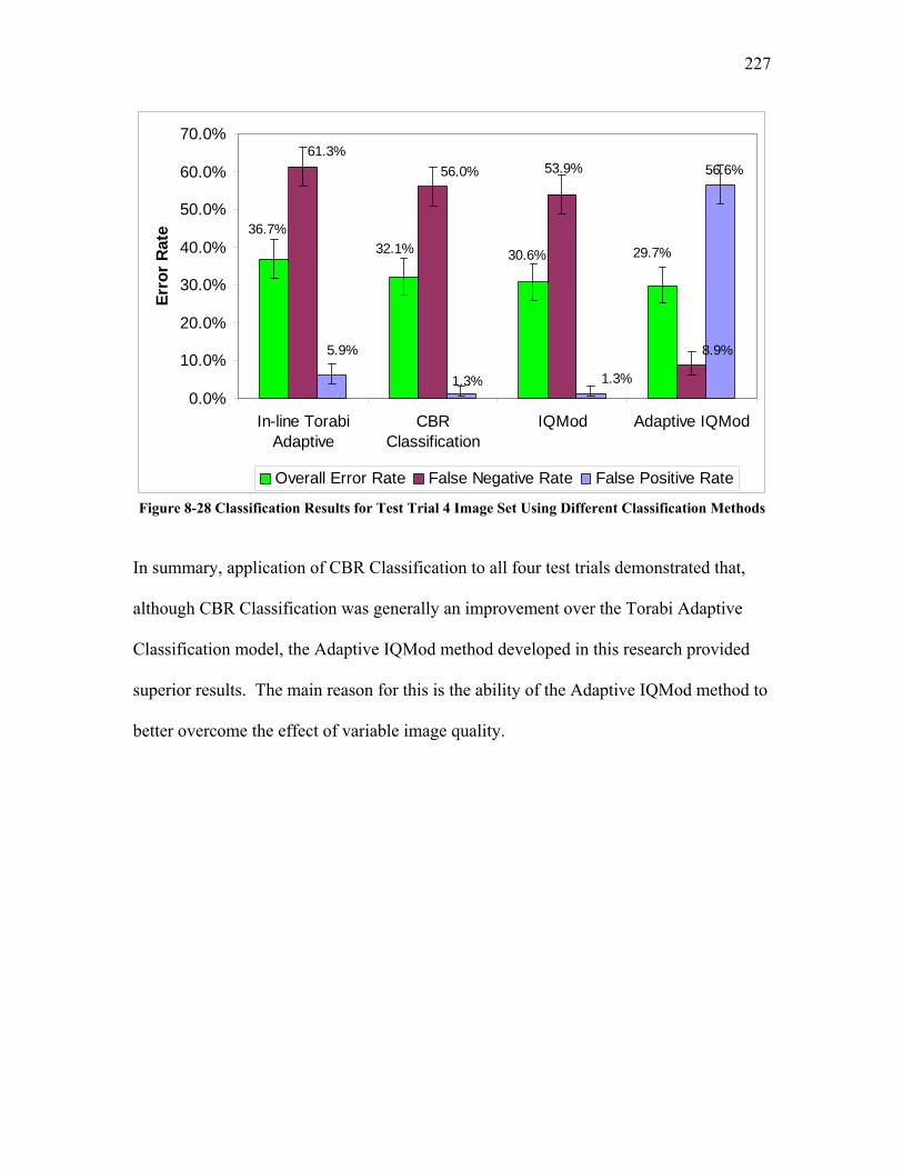
227
29.7%30.6%
36.7%32.1%
56.0% 53.9%61.3%
8.9%
56.6%
1.3% 1.3%
5.9%
0.0%
10.0%
20.0%
30.0%
40.0%
50.0%
60.0%
70.0%
In-line TorabiAdaptive
CBRClassification
IQMod Adaptive IQMod
Erro
r R
ate
Overall Error Rate False Negative Rate False Positive Rate
Figure 8-28 Classification Results for Test Trial 4 Image Set Using Different Classification Methods
In summary, application of CBR Classification to all four test trials demonstrated that,
although CBR Classification was generally an improvement over the Torabi Adaptive
Classification model, the Adaptive IQMod method developed in this research provided
superior results. The main reason for this is the ability of the Adaptive IQMod method to
better overcome the effect of variable image quality.
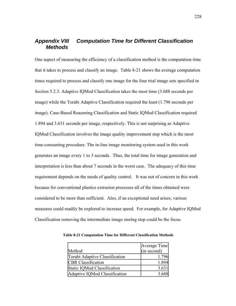
228
Appendix VIII Computation Time for Different Classification Methods
One aspect of measuring the efficiency of a classification method is the computation time
that it takes to process and classify an image. Table 8-21 shows the average computation
times required to process and classify one image for the four trial image sets specified in
Section 5.2.3. Adaptive IQMod Classification takes the most time (3.688 seconds per
image) while the Torabi Adaptive Classification required the least (1.796 seconds per
image). Case-Based Reasoning Classification and Static IQMod Classification required
1.894 and 3.631 seconds per image, respectively. This is not surprising as Adaptive
IQMod Classification involves the image quality improvement step which is the most
time-consuming procedure. The in-line image monitoring system used in this work
generates an image every 1 to 3 seconds. Thus, the total time for image generation and
interpretation is less than about 7 seconds in the worst case. The adequacy of this time
requirement depends on the needs of quality control. It was not of concern in this work
because for conventional plastics extrusion processes all of the times obtained were
considered to be more than sufficient. Also, if an exceptional need arises, various
measures could readily be explored to increase speed. For example, for Adaptive IQMod
Classification removing the intermediate image storing step could be the focus.
Table 8-21 Computation Time for Different Classification Methods
Method Average Time (in second)
Torabi Adaptive Classification 1.796 CBR Classification 1.894 Static IQMod Classification 3.631 Adaptive IQMod Classification 3.688

229
Appendix IX Statistics on the Estimation of Proportions There is a need to determine how certain we are about the classification error rates
obtained for a set of images. In this thesis, this is accomplished by computing a
confidence interval. This appendix details how that was done.
For the training images, ten fold cross validation was done each time a model was
formulated. A total of 745 images were used. So, nine folds (i.e., 90% or 671 of 745
images) in the cross validation fitted the model and obtained the error rate when the
remaining fold of 74 images were classified using this model. The process was repeated
ten times using a different 74 image group each time. The error rates obtained for the
different models arising out of using different image quality definitions to optimize the
images to be classified is shown in Table 8-22 .
Table 8-22 Errors from 10-Fold Cross Validation for Classification Models Created Based on Images Optimized Using Different Image Quality Definitions
Origin of Data Raw LS WLS DF PD Fold 1 6 2 1 1 1 Fold 2 4 2 3 2 0 Fold 3 3 1 2 1 0 Fold 4 5 1 1 1 0 Fold 5 7 3 2 2 0 Fold 6 5 2 1 1 0 Fold 7 3 0 0 0 0 Fold 8 2 0 2 1 0 Fold 9 3 1 0 2 0 Fold 10 3 1 2 2 0 Average Number of Errors 4.1 1.3 1.4 1.3 0.1 Standard Deviation 1.60 0.95 0.97 0.67 0.32 Total Number of Errors 41 13 14 13 1
Notes: Raw – Raw Images, LS – Least Squares Optimized Images, WLS—Weighted Least Squares Optimized Images, DF – Desirability Function Optimized Images, PD – Probability Density Difference Optimized Images.

230
By inspection of this table it can be seen that the probability density difference definition
of image quality obviously has the lowest error rate. Quantifying precision beyond the
information shown in Table 8-22 using confidence intervals encounters some uncertainty
because the error rates cannot really be considered as statistically independent quantities
[145]: in the cross validation process, calculation of each error rate uses many of the raw
images that were used for the other error rates. Also, when only ten error rates are used
in a confidence interval calculation, the conventional approach is to use the Students t
distribution. That calculation requires that the error rates be normally distributed. When
as many as 30 error rates are used then the Central Limit Theorem is applicable and often
the distribution of sample mean error rates can be considered normally distributed: then
the standard normal variate, z, can be used instead of t.
Confidence intervals (or, hypothesis tests which involve essentially the same
calculations) are conventionally used in data mining research and are calculated not from
the error rates but from a theoretical equation [110, 146]. That equation assumes that the
error rates obey a binomial distribution which can be approximated by a Normal
distribution. The approach is very convenient for test images since cross validation is
only carried out in the training step and so, error rates from cross validation are not
available. Closer examination of this method revealed that the most common method of
calculating the theoretical intervals is based upon yet another approximation [146].
When that approximation is used, the confidence interval is symmetric about the average
error rate. When it is not used then the interval is asymmetric. Despite the popularity of
the symmetric interval equation, in a comparison of these two theoretical equations [146],
the asymmetric interval was found to provide a very significantly superior estimate of the

231
confidence interval. Since the asymmetric theoretical equation was used in this work for
obtaining all confidence intervals shown in the bar graphs throughout the thesis, further
details, including a sample calculation, will be shown below. However before
progressing to that, Figure 8-29 shows a comparison of the various confidence intervals
including those calculated using the cross validation error rates of Table 8-22 for the
various classification models resulting from different image quality definitions. It can be
seen in Figure 8-23 that the asymmetric, theoretical confidence interval consistently
provided the most pessimistic view of the data.
Figure 8-29 Comparison of Confidence Intervals
0.0%
1.0%
2.0%
3.0%
4.0%
5.0%
6.0%
7.0%
8.0%
TorabiBayesian
Model
LeastSquares
WeightedLeast
Squares
DesirabilityFunction
ProbabilityDensity
Difference
Erro
r Rat
e (%
)
Asymmetric Approximated CI Symmetric Approximated CIT-Distribution CI Z-Distribution CI
Now, the calculation of the symmetric and asymmetric theoretical confidence intervals
will be described. The data of Table 8-23 will be used to illustrate the calculation. This
data shows typical results of the classification of a set of images.

232
Table 8-23 A Sample Classification Confusion Matrix
Predicted Class is WP Predicted Class is WO
Actual Class is WP 489 16 Actual Class is WO 25 215
From Table 8-23 , the total number of images in the sample (i.e. the sample size, n) is:
n = 489+16+25+215 = 745
The classification error rate, e, is given by: e= y/n= (16+25)/745 = 0.055
where y is the total number of misclassified images.
It is known that the proportion, e, follows binomial distributions. However, if ne > 5
when e ≤ 0.5 or if n (1-e) > 5 when e ≥ 0.5, then the binomial distribution can be
approximated by a normal distribution with a mean of ne and a standard deviation of (ne
(1-e))0.5. That is N(ne,(ne(1-e))0.5) ~ N(µ, σ). With this assumption, the calculation of the
standard normal variate, z, for an observation of y misclassified images is given by
)1( eneneyz−
−= 8-67
where e is the true classification error rate, y is the number of misclassified images and n
is the sample size. z then follows a standard normal distribution (a normal distribution
with a mean of zero and standard deviation of 1), that is, it is N(0,1).
The above equation can be rewritten as:
nee
enyz/)1(
/−
−= 8-68

233
Solving the above equation for e gives “asymmetric confidence interval” equation (termed the “score confidence interval” [146]):
nz
nz
ny
nyz
nz
ny
e 2
2
2
3
2
2
2
1
42
+
+−±+= 8-69
The value of z for the 95% confidence level is obtained using a z table; it is 1.96. The
lower limit of the confidence interval is calculated as substituting the appropriate values
of the variables into the equation:
0408.0
74596.11
745496.1
74541
7454196.1
745296.1
74541
2
2
2
3
2
2
2
=+
×+−−
×+
The upper limit is:
0738.0
74596.11
745496.1
74541
7454196.1
745296.1
74541
2
2
2
3
2
2
2
=+
×+−+
×+
The estimate of the 95% confidence interval is therefore:
0.0408 ≤ e ≤ 0.0738. We are 95% confident that the “actual” error rate is in that range.
More accurately, the meaning of this 95% confidence interval is as follows:
If 1000 samples of 745 images each were obtained and the 95% confidence interval
calculated as above for each one of these samples, about 950 of these confidence
intervals would contain the population mean of the error rate (the “actual” error rate) and
about 50 would not.
234
An approximate form of Eqn. 8-68 frequently used in data mining applications can be
obtained from Eqn. 8-69 by first writing this equation as:
neez
nye )1(
2/−
±= α 8-70
and then approximating the true error rate (the population mean error rate) on the right
hand side of the equation by the observed error rate, y/n, to obtain the symmetric
confidence interval equation (termed the Wald confidence interval [146]):
nny
ny
znye
)1(2/
−±= α 8-71
Now, repeating the above numerical example using Eqn. 8-70 we obtain:
745
)745411(
74541
96.174541 −
±=e
The 95% confidence limits are: 0.00387, 0.0714. For this specific example then, the
values obtained represent about a 5% and 3% deviation respectively from the values
obtained from the first, more exact, equation. In this thesis all results were calculated
using Equation 8-69.
235
9 REFERENCES 1. Torabi, K., S. Sayad, and S.T. Balke, On-line Adaptive Bayesian Classification
for In-line Particle Image Monitoring in Polymer Film Manufacturing. Computers and Chemical Engineering, 2005.
2. Torabi, K., Data Mining Methods for Quantitative In-line Image Monitoring in Polymer Extrusion, Ph.D. Thesis, Department of Chemical Engineering and Applied Chemistry. University of Toronto: Toronto, ON, Canada. 2005
3. Baykut, A., et al., Real-time Defect Inspection of Textured Surfaces. Real-Time Imaging, 2000. 6(1): p. 17-27.
4. Bharati, M.H. and J.F. MacGregor, Multivariate image analysis for real-time process monitoring and control. Industrial & Engineering Chemistry Research, 1998. 37(12): p. 4715-4724.
5. Bharati, M.H., J.F. MacGregor, and W. Tropper, Softwood lumber grading through on-line multivariate image analysis techniques. Industrial & Engineering Chemistry Research, 2003. 42(21): p. 5345-5353.
6. Darwish, A.M. and A.K. Jain, A rule based approach for visual pattern inspection. Pattern Analysis and Machine Intelligence, IEEE Transactions on, 1988. 10(1): p. 56-68.
7. Farahani, F., et al. In-line color monitoring during polyethylene extrusion: Reflectance spectra and images. in 61st Annual Technical Conference ANTEC 2003. 2003. Nashville, TN, United States.
8. Gilmor, C., et al., In-Line Color Monitoring of Polymers During Extrusion Using a Charge Coupled Device Spectrometer: Color Changeovers and Residence Time Distributions. Polymer Engineering and Science, 2003. 43(2): p. 356-368.
9. Joeris, K., et al., In-situ microscopy: Online process monitoring of mammalian cell cultures. Cytotechnology, 2002. 38(1-2): p. 129-134.
10. Persoon, E., A pipelined image analysis system using custom integrated circuits. Pattern Analysis and Machine Intelligence, IEEE Transactions on, 1988. 10(1): p. 110-116.
11. Reshadat, R., et al. In-line color monitoring of pigmented polyolefins during extrusion I: assessment. in Proceedings of the 1996 54th Annual Technical Conference. 1996. Part 3 (of 3). Indianapolis, IN.
12. Sayad, S., et al. In-line color monitoring of pigmented polyolefins during extrusion II: color prediction. in Proceedings of the 1996 54th Annual Technical Conference. 1996. Part 3 (of 3). Indianapolis, IN.
13. Torabi, K., et al. Data mining for image analysis: in-line particle monitoring in polymer extrusion. in Third International Conference on Data Mining. Data Mining III. 2002. Bologna, Italy: WIT Press.
14. Wang, H. and R. Kovacevic, On-line monitoring of the keyhole welding pool in variable polarity plasma arc welding. Proceedings of the Institution of Mechanical Engineers Part B-Journal of Engineering Manufacture, 2002. 216(9): p. 1265-1276.

236
15. Watano, S., et al., On-line monitoring of granule growth in high shear granulation by an image processing system. Chemical & Pharmaceutical Bulletin, 2000. 48(8): p. 1154-1159.
16. Yoda, H., et al., An automatic wafer inspection system using pipelined image processing techniques. Pattern Analysis and Machine Intelligence, IEEE Transactions on, 1988. 10(1): p. 4-16.
17. Yu, K., J.A. Phillips, and A.J. Rein, Online Monitoring and Control of Escherichia-Coli Fermentation with Ftir/Atr Spectroscopy Implemented on a Pilot-Scale Fermenter. Abstracts of Papers of the American Chemical Society, 1994. 207: p. 100-BIOT.
18. Yu, H.L., et al., Digital imaging for online monitoring and control of industrial snack food processes. Industrial & Engineering Chemistry Research, 2003. 42(13): p. 3036-3044.
19. Ing, L. and S.T. Balke. In-line Measurement of Dispersed Phase Properties Using The Scanning Particle Monitor. in ANTEC 2002. 2002. San Francisco.
20. Sayad, S. and S.T. Balke. An intelligent learning machine. in Fourth International Conference on Data Mining, Data Mining IV. 2003. Rio De Janeiro, Brazil: Wessex Institute of Technology; COPPE/Federal University of Rio de Janeiro.
21. Dieterle, F., S. Busche, and G. Gauglitz, Growing neural networks for a multivariate calibration and variable selection of time-resolved measurements. Analytica Chimica Acta, 2003. 490(1-2): p. 71-83.
22. An, J.-L., Z.-O. Wang, and Z.-P. Ma. An incremental learning algorithm for support vector machine. in Machine Learning and Cybernetics, 2003 International Conference on. 2003.
23. Mouchaweh, M.S., et al., Incremental learning in Fuzzy Pattern Matching. Fuzzy Sets and Systems, 2002. 132(1): p. 49-62.
24. Bruzzone, L. and D. Fernàndez Prieto, An incremental-learning neural network for the classification of remote-sensing images. Pattern Recognition Letters, 1999. 20(11-13): p. 1241-1248.
25. Freund, Y. and R.E. Schapire, A Decision-Theoretic Generalization of On-Line Learning and an Application to Boosting. Journal of Computer and System Sciences, 1997. 55(1): p. 119-139.
26. Wienke, D., et al., Adaptive resonance theory based neural network for supervised chemical pattern recognition (FuzzyARTMAP) .2. Classification of post-consumer plastics by remote NIR spectroscopy using an InGaAs diode array. Chemometrics and Intelligent Laboratory Systems, 1996. 32(2): p. 165-176.
27. Wienke, D. and L. Buydens, Adaptive resonance theory based neural network for supervised chemical pattern recognition (FuzzyARTMAP) .1. Theory and network properties. Chemometrics and Intelligent Laboratory Systems, 1996. 32(2): p. 151-164.
28. Fu, L., H.-H. Hsu, and J.C. Principe, Incremental backpropagation learning networks. Neural Networks, IEEE Transactions on, 1996. 7(3): p. 757-761.
29. Wienke, D. and D.L. Buydens, Adaptive resonance theory based neural networks -- the ‘ART’ of real-time pattern recognition in chemical process monitoring? TrAC - Trends in Analytical Chemistry, 1995. 14(1): p. 398-406.
237
30. Carpenter, G.A., et al., Fuzzy ARTMAP: A neural network architecture for incremental supervised learning of analog multidimensional maps. Neural Networks, IEEE Transactions on, 1992. 3(5): p. 698-713.
31. Park, D.C., M.A. El-Sharkawi, and R.J. Marks, II, An adaptively trained neural network. Neural Networks, IEEE Transactions on, 1991. 2(3): p. 334-345.
32. Carpenter, G.A., S. Grossberg, and J.H. Reynolds, ARTMAP: Supervised real-time learning and classification of nonstationary data by a self-organizing neural network. Neural Networks, 1991. 4(5): p. 565-588.
33. Torabi, K., S. Sayad, and S.T. Balke, On-line adaptive Bayesian classification for in-line particle image monitoring in polymer film manufacturing. Computers & Chemical Engineering, 2005. 30(1): p. 18-27.
34. Avcibas, I., B. Sankur, and K. Sayood, Statistical evaluation of image quality measures. J. Electron. Imaging, 2002. 11(2): p. 206-223.
35. Eskicioglu Ahmet, M. Quality measurement for monochrome compressed images in the past 25 years. in 2000 IEEE Interntional Conference on Acoustics, Speech, and Signal Processing. 2000. Istanbul, Turkey: Ieee.
36. Fiete, R.D. and T. Tantalo, Comparison of SNR image quality metrics for remote sensing systems. 2001. 40(4): p. 574-585.
37. Jacobson, R.E., An Evaluation of Image Quality Metrics. J. Photogr. Sci., 1995. 43(1): p. 7-16.
38. Shnayderman, A., A. Gusev, and M. Eskicioglu Ahmet. A multidimensional image quality measure using Singluar Value Decomposition. in Image Quality and System Performance. 2004. San Jose, California, USA: SPIE and IS&T.
39. Veldkamp, W.J.H. and N. Karssemeijer, Normalization of local contrast in mammograms. Medical Imaging, IEEE Transactions on, 2000. 19(7): p. 731-738.
40. Wang, Z. and A.C. Bovik, A universal image quality index. IEEE Signal Processing Letters, 2002. 9(3): p. 81.
41. Wang, Z., L. Lu, and A.C. Bovik, Video quality assessment based on structural distortion measurement. Signal Processing: Image Communication, 2004. 19(2): p. 121-132.
42. Wang, Z., H.R. Sheikh, and A.C. Bovik. No-reference perceptual quality assessment of JPEG compressed images. in Proceedings of ICIP 2002 International Conference on Image Processing. 2002. Piscataway, NJ, USA: IEEE.
43. Xu, W. and G. Hauske, Picture quality evaluation based on error segmentation. Proceedings of SPIE The International Society for Optical Engineering, 1994. 2308: p. 1454-1465.
44. Eskicioglu Ahmet, M. and S. Fisher Paul, Image quality measures and their performance. IEEE Transactions on Communications, 1995. 43(12): p. 2959-2965.
45. Aach, T., U. Schiebel, and G. Spekowius, Digital image acquisition and processing in medical x-ray imaging. Journal of Electronic Imaging, 1999. 8(1): p. 7-22.
46. Li, X. Blind image quality assessment. in Image Processing. 2002. Proceedings. 2002 International Conference on. 2002.

238
47. Caviedes, J. and S. Gurbuz. No-reference sharpness metric based on local edge kurtosis. in Proceedings of ICIP 2002 International Conference on Image Processing. 2002. Piscataway, NJ, USA: IEEE.
48. Turaga, D.S., Y. Chen, and J. Caviedes, No reference PSNR estimation for compressed pictures. Signal Processing: Image Communication, 2004. 19(2): p. 173-184.
49. Bojkovic, Z., Image quality estimation in subband coding techniques based on human visual system. International Conference on Communication Technology Proceedings, ICCT, 1996. 2: p. 651-653.
50. Caviedes, J. and F. Oberti, A new sharpness metric based on local kurtosis, edge and energy information. Signal Processing-Image Communication, 2004. 19(2): p. 147-161.
51. Siew, L.H., R.M. Hodgson, and E.J. Wood, Texture measures for carpet wear assessment. Pattern Analysis and Machine Intelligence, IEEE Transactions on, 1988. 10(1): p. 92-105.
52. Gonzalez, R.C. and R.E. Woods, Digital Image Processing. 2002, Upper Saddle River, N.J.: Prentice Hall.
53. Blatt, R.J., et al., Automated quantitative analysis of angiogenesis in the rat aorta model using image-pro plus 4.1. Computer Methods and Programs in Biomedicine, 2004. 75(1): p. 75-79.
54. Belien, J.A.M., et al., Fully automated microvessel counting and hot spot selection by image processing of whole tumour sections in invasive breast cancer. Journal of Clinical Pathology, 1999. 52(3): p. 184-192.
55. Beksac, M.S., et al., An automated intelligent diagnostic system for the interpretation of umbilical artery Doppler velocimetry. European Journal of Radiology, 1996. 23(2): p. 162-167.
56. Zalewski, K. and R. Buchholz, Morphological analysis of yeast cells using an automated image processing system. Journal of Biotechnology, 1996. 48(1-2): p. 43-49.
57. Yeasin, M. and S. Chaudhuri, Development of an automated image processing system for kinematic analysis of human gait. Real-Time Imaging, 2000. 6(1): p. 55-67.
58. Wit, P. and H.J. Busscher, Application of an artificial neural network in the enumeration of yeasts and bacteria adhering to solid substrata. Journal of Microbiological Methods, 1998. 32(3): p. 281-290.
59. Tanaka, M. and A. Kayama, Automated image processing for fractal analysis of fracture surface profiles in high-temperature materials. Journal of Materials Science Letters, 2001. 20(10): p. 907-909.
60. Petropoulos, H., W.L. Sibbitt, and W.M. Brooks, Automated T-2 quantitation in neuropsychiatric lupus erythematosus: A marker of active disease. Journal of Magnetic Resonance Imaging, 1999. 9(1): p. 39-43.
61. Mahadevan, S. and D. Casasent, Automated image processing for grain boundary analysis. Ultramicroscopy, 2003. 96(2): p. 153-162.
62. Kuklin, A., S. Shams, and S. Shah, High throughput screening of gene expression signatures. Genetica, 2000. 108(1): p. 41-46.
239
63. Krooshoop, D., et al., An automated multi well cell track system to study leukocyte migration. Journal of Immunological Methods, 2003. 280(1-2): p. 89-102.
64. Gong, L., et al. Knowledge-based remote image processing and compression for efficient transmission. in Proceedings of the 1995 IS and T's 48th Annual Conference. 1995. Washington, DC: Is&t.
65. Chien, S.A. and H.B. Mortensen, Automating image processing for scientific data analysis of a large image database. Pattern Analysis and Machine Intelligence, IEEE Transactions on, 1996. 18(8): p. 854-859.
66. Clement, V. and M. Thonnat, A Knowledge-Based Approach to Integration of Image Processing Procedures. CVGIP: Image Understanding, 1993. 57(2): p. 166 - 184.
67. Clouard, R., et al., Borg: a knowledge-based system for automatic generation of image processing programs. IEEE Transactions on Pattern Analysis and Machine Intelligence, 1999. 21(2): p. 128-144.
68. Gong, L. and A. Kulikowski Casimir, Composition of image analysis processes through object-centered hierarchical planning. IEEE Transactions on Pattern Analysis and Machine Intelligence, 1995. 17(10): p. 997-1009.
69. Grimm, F. and H. Bunke, Expert system for the selection and application of image processing subroutines. Expert Systems, 1993. 10(2): p. 61-74.
70. Matsuyama, T. Expert systems for image processing - knowledge-based composition of image analysis processes. in 9th International Conference on Pattern Recognition. 1988. Rome, Italy: Int Assoc for Pattern Recognition, Paris, Fr.
71. Toriu, T., H. Iwase, and M. Yoshida, Expert System for Image Processing. Fujitsu Sci Tech J, 1987. 23(2): p. 111-118.
72. Tanaka, T. and N. Sueda. Knowledge acquisition in image processing expert system 'EXPLAIN'. in Proceedings of the International Workshop on Artificial Intelligence for Industrial Applications. 1988. Hitachi, Jpn: IEEE, Industrial Electronics Soc, New York, NY, USA.
73. Aha, D.W., C. Marling, and I. Watson, Case-based reasoning commentaries: introduction. Knowledge Engineering Review, 2005. 20(3): p. 201-202.
74. Holt, A., et al., Medical applications in case-based reasoning. Knowledge Engineering Review, 2005. 20(3): p. 289-292.
75. Rissland, E.L., K.D. Ashley, and L.K. Branting, Case-based reasoning and law. Knowledge Engineering Review, 2005. 20(3): p. 293-298.
76. Kolodner, J.L., M.T. Cox, and P.A. Gonzalez-Caler, Case-based reasoning-inspired approaches to education. Knowledge Engineering Review, 2005. 20(3): p. 299-303.
77. Althoff, K.D. and R.O. Weber, Knowledge management in case-based reasoning. Knowledge Engineering Review, 2005. 20(3): p. 305-310.
78. Ficet-Cauchard, V., C. Porquet, and M. Revenu, CBR for the management and reuse of image-processing expertise: a conversational system. Engineering Applications of Artificial Intelligence, 1999. 12(6): p. 733-747.
79. Perner, P., A. Holt, and M. Richter, Image processing in case-based reasoning. Knowledge Engineering Review, 2005. 20(3): p. 311-314.
240
80. Perner, P., An architecture for a CBR image segmentation system, in Case-Based Reasoning Research and Development. 1999. p. 525-534.
81. Ficet-Cauchard, V., C. Porquet, and M. Revenu, An interactive case-based reasoning system for the development of image processing applications, in Advances in Case-Based Reasoning. 1998. p. 437-447.
82. Grimnes, M. and A. Aamodt, A two layer case-based reasoning architecture for medical image understanding, in Advances in Case-Based Reasoning. 1996. p. 164-178.
83. Jarmulak, J., E.J.H. Kerckhoffs, and P.P. van't Veen, Case-based reasoning in an ultrasonic rail-inspection system, in Case-Based Reasoning Research and Development. 1997. p. 43-52.
84. Perner, P., CBR-based ultra sonic image interpretation, in Advances in Case-Based Reasoning, Proceedings. 2001. p. 479-490.
85. Macura, R.T., et al., Computerized Case-Based Instructional-System for Computed-Tomography and Magnetic-Resonance-Imaging of Brain-Tumors. Investigative Radiology, 1994. 29(4): p. 497-506.
86. Cheetham, W. and I. Watson, Fielded applications of case-based reasoning. Knowledge Engineering Review, 2005. 20(3): p. 321-323.
87. Hinkle, D. and C. Toomey, Applying Case-Based Reasoning to Manufacturing. Ai Magazine, 1995. 16(1): p. 65-73.
88. Heider, R., Troubleshooting CFM56-3 engines for the Boeing737 using a CBR and data-mining, in Advances in Case-Based Reasoning. 1996. p. 512-518.
89. Cheetham, W. and J. Graf, Case-based reasoning in color matching, in Case-Based Reasoning Research and Development. 1997. p. 1-12.
90. Watson, I. and D. Gardingen, A Distributed Case-Based Reasoning Application for Engineering Sales Support in Proceedings of the Sixteenth International Joint Conference on Artificial Intelligence 1999 Morgan Kaufmann Publishers Inc. p. 600-605
91. Varma, A. and N. Roddy, ICARUS: design and deployment of a case-based reasoning system for locomotive diagnostics. Engineering Applications of Artificial Intelligence, 1999. 12(6): p. 681-690.
92. Jurisica, I. and J. Glasgow, Applications of case-based reasoning in molecular biology. Ai Magazine, 2004. 25(1): p. 85-95.
93. Perner, P., Why case-based reasoning is attractive for image interpretation, in Case-Based Reasoning Research and Development, Proceedings. 2001. p. 27-43.
94. Jabbour, K., et al., Alfa - Automated Load Forecasting Assistant. Ieee Transactions on Power Systems, 1988. 3(3): p. 908-914.
95. Bartels, P.H., T. Gahm, and D. Thompson, Automated microscopy in diagnostic histopathology: From image processing to automated reasoning. International Journal of Imaging Systems and Technology, 1997. 8(2): p. 214-223.
96. Haddad, M., K.P. Adlassnig, and G. Porenta, Feasibility analysis of a case-based reasoning system for automated detection of coronary heart disease from myocardial scintigrams. Artificial Intelligence in Medicine, 1997. 9(1): p. 61-78.
97. Jarmulak, J., Case-based classification of ultrasonic B-scans: Case-base organisation and case retrieval, in Advances in Case-Based Reasoning. 1998. p. 100-111.

241
98. Leake, D.B., Case-Based Reasoning: Experiences, Lessons, and Future Directions. 1996, Menlo Park: AAAI Press/MIT Press.
99. Aamodt, A. and E. Plaza, Case-Based Reasoning - Foundational Issues, Methodological Variations, and System Approaches. Ai Communications, 1994. 7(1): p. 39-59.
100. De Mantaras, R.L., et al., Retrieval, reuse, revision and retention in case-based reasoning. Knowledge Engineering Review, 2005. 20(3): p. 215-240.
101. Perner, P., Are case-based reasoning and dissimilarity-based classification two sides of the same coin? Engineering Applications of Artificial Intelligence, 2002. 15(2): p. 193-203.
102. Zamperoni, P. and V. Starovoitov. How dissimilar are two gray-scale images. in DAGM. 1995. Berlin, Germany: Springer.
103. Santini, S. and R. Jain, Similarity measures. Ieee Transactions on Pattern Analysis and Machine Intelligence, 1999. 21(9): p. 871-883.
104. Perner, P., Content-Based Image Indexing and Retrieval in an Image Database for Technical Domains, in Lecture Notes in Computer Science, H.S. Smuelder, Editor. 1998, Springer: Berlin. p. 207-224.
105. Tsai, C.-Y., C.-C. Chiu, and J.-S. Chen, A case-based reasoning system for PCB defect prediction. Expert Systems With Applications, 2005. 28(4): p. 813-822.
106. Perner, P., Using CBR Learning for the Low-Level and Highlevel Unit of an Image Interpretation System, in Advances in Pattern Recognition, S. Singh, Editor. 1998, Springer: Berlin. p. 45-54.
107. McSherry, D., Precision and recall in interactive case-based reasoning, in Case-Based Reasoning Research and Development, Proceedings. 2001. p. 392-406.
108. Bailey, T.L. and C. Elkan. Estimating the accuracy of learned concepts. in International Joint Conference on Artificial Intelligence. 1993: Morgan Kaufmann Publisher.
109. Breiman, L. and P. Spector, Submodel Selection and Evaluation in Regression - the X-Random Case. International Statistical Review, 1992. 60(3): p. 291-319.
110. Kohavi, R. A study of cross-validation and bootstrap for accuracy estimation and model selection. in Proceedings of International Joint Conference on Artificial Intelligence. 1995. Montreal, Que., Canada.
111. Domingos, P. and M. Pazzani, On the optimality of the simple Bayesian classifier under zero-one loss. Machine Learning, 1997. 29(2-3): p. 103-130.
112. Rish, I. An empirical study of the naive Bayes classifier. in International Joint Conference on Artificial Intelligence. 2001.
113. Peli, E., In search of a contrast metric: Matching the perceived contrast of Gabor patches at different phases and bandwidths. Vision Research, 1997. 37(23): p. 3217-3224.
114. McLoughlin, K.J., P.J. Bones, and N. Karssemeijer, Noise equalization for detection of microcalcification clusters in direct digital mammogram images. Medical Imaging, IEEE Transactions on, 2004. 23(3): p. 313-320.
115. Zhang, D. and Z. Wang, Impulse noise detection and removal using fuzzy techniques. Electronics Letters, 1997. 33(5): p. 378-379.
116. Chen, T.-J., et al., A novel image quality index using Moran I statistics. Physics in Medicine and Biology, 2003. 48(8): p. N131.
242
117. Zhang, N.F., et al., Image sharpness measurement in the scanning electron microscope - Part III. Scanning, 1999. 21(4): p. 246-252.
118. Marziliano, P., et al. A no-reference perceptual blur metric. in Proceedings of ICIP 2002 International Conference on Image Processing. 2002. Piscataway, NJ, USA: IEEE.
119. Puttenstein, J.G., I. Heynderickx, and G. de Haan, Evaluation of objective quality measures for noise reduction in TV-systems. Signal Processing: Image Communication, 2004. 19(2): p. 109-119.
120. Venetsanopoulos, A., Digital Image Processing and Applications. 2002: Toronto. 121. Seul, M., L. O'Gorman, and M.J. Sammon, Practical Algorithms for image
Analysis. 2000, Cambridge, UK: Cambridge University Press. 122. Davies, E., Machine Vision: theory, Algorithms, practicalities. 1997, Academic
Press: San Diego. 123. Olsson, D.M. and L.S. Nelson, Nelder-Mead Simplex Procedure for Function
Minimization. Technometrics, 1975. 17(1): p. 45-51. 124. Walters, F., Sequential simplex optimization - An update. Analytical Letters,
1999. 32(2): p. 193-+. 125. Walters, F.H., et al., Sequential Simplex Optimisation. 1991, Boca Raton, Florida:
CRC Press LLC. 126. Routh, M.W., P.A. Swartz, and M.B. Denton, Performance of the super modified
simplex. Analytical Chemistry, 1977. 49(9): p. 1422-1428. 127. Betteridge, D., A.P. Wade, and A.G. Howard, Reflections on the modified
simplex--I. Talanta, 1985. 32(8, Part 2): p. 709-722. 128. Betteridge, D., A.P. Wade, and A.G. Howard, Reflections on the modified
simplex--II. Talanta, 1985. 32(8, Part 2): p. 723-734. 129. Kelley, C.T., Detection and remediation of stagnation in the Nelder-Mead
algorithm using a sufficient decrease condition. Siam Journal on Optimization, 1999. 10(1): p. 43-55.
130. Barton, R.R. and J.S. Ivey, Nelder-Mead simplex modifications for simulation optimization. Management Science, 1996. 42(7): p. 954-973.
131. Syed, N., H. Liu, and K. Sung. Incremental Learning with Support Vector Machines. in International Joint Conference on Artificial Intelligence. 1999. Stockholm, Sweden.
132. Carozza, M. and S. Rampone. Towards an incremental SVM for regression. in Neural Networks, 2000. IJCNN 2000, Proceedings of the IEEE-INNS-ENNS International Joint Conference on. 2000.
133. Xiao, R., J. Wang, and F. Zhang. An approach to incremental SVM learning algorithm. in Tools with Artificial Intelligence, 2000. ICTAI 2000. Proceedings. 12th IEEE International Conference on. 2000.
134. Cauwenberghs, G. and T. Poggio, Incremental and Decremental Support Vector Machine Learning, in Advances in Neural Information Processing Systems. 2001, MIT Press.
135. Li, K. and H.-K. Huang. Incremental learning proximal support vector machine classifiers. in Machine Learning and Cybernetics, 2002. Proceedings. 2002 International Conference on. 2002.
136. Martin, M., On-line Support Vector Machines for Function Approximation. 2002.
243
137. Peng, B., X. Sun Zheng, and G. Xu Xiao. SVM-based incremental active learning for user adaptation for online graphics recognition system. in Proceedings of 2002 International Conference on Machine Learning and Cybernetics. 2002. Beijing, China: Hebei University; IEEE systems, Man and Cybernetics technical Comm. on Cybernetics.
138. Diehl Christopher, P. and G. Cauwenberghs. SVM Incremental Learning, Adaptation and Optimization. in International Joint Conference on Neural Networks 2003. 2003. Portland, OR, United States: The International Neural Network Society; The IEEE Neural Network Society.
139. Chakraborty, D. and N.R. Pal, A novel training scheme for multilayered perceptrons to realize proper generalization and incremental learning. Ieee Transactions on Neural Networks, 2003. 14(1): p. 1-14.
140. Sato, M. and S. Ishii, On-line EM algorithm for the normalized gaussian network. Neural Computation, 2000. 12(2): p. 407-432.
141. Schaal, S. and C.G. Atkeson, Constructive incremental learning from only local information. Neural Computation, 1998. 10(8): p. 2047-2084.
142. Schaal, S., C.G. Atkeson, and S.V. Vijayakumar, Scalable techniques from nonparametric statistics for real time robot learning. Applied Intelligence, 2002. 17(1): p. 49-60.
143. Su, J.B., J. Wang, and Y.G. Xi, Incremental learning with balanced update on receptive fields for multi-sensor data fusion. Ieee Transactions on Systems Man and Cybernetics Part B-Cybernetics, 2004. 34(1): p. 659-665.
144. Sugiyama, M. and H. Ogawa, Incremental construction of projection generalizing neural networks. Ieice Transactions on Information and Systems, 2002. E85D(9): p. 1433-1442.
145. Bengio, Y. and Y. Grandvalet, No unbiased estimator of the variance of K-fold cross-validation. Journal of Machine Learning Research, 2004. 5: p. 1089-1105.
146. Agresti, A. and B.A. Coull, Approximate is better than "exact" for interval estimation of binomial proportions. The American Statistician, 1998. 52(2): p. 119.