Embed Size (px)
Citation preview
IEEE TRANSACTIONS ON IMAGE PROCESSING, VOL. 22, NO. 1, JANUARY 2013 5
Adaptive Markov Random Fields forJoint Unmixing and Segmentation
of Hyperspectral ImagesOlivier Eches, Jón Atli Benediktsson, Fellow, IEEE, Nicolas Dobigeon, Member, IEEE, and
Jean-Yves Tourneret, Senior Member, IEEE
Abstract— Linear spectral unmixing is a challenging problemin hyperspectral imaging that consists of decomposing anobserved pixel into a linear combination of pure spectra (or end-members) with their corresponding proportions (or abundances).Endmember extraction algorithms can be employed for recov-ering the spectral signatures while abundances are estimatedusing an inversion step. Recent works have shown that exploitingspatial dependencies between image pixels can improve spectralunmixing. Markov random fields (MRF) are classically usedto model these spatial correlations and partition the imageinto multiple classes with homogeneous abundances. This paperproposes to define the MRF sites using similarity regions. Theseregions are built using a self-complementary area filter thatstems from the morphological theory. This kind of filter dividesthe original image into flat zones where the underlying pixelshave the same spectral values. Once the MRF has been clearlyestablished, a hierarchical Bayesian algorithm is proposed toestimate the abundances, the class labels, the noise variance, andthe corresponding hyperparameters. A hybrid Gibbs sampler isconstructed to generate samples according to the correspondingposterior distribution of the unknown parameters and hyperpa-rameters. Simulations conducted on synthetic and real AVIRISdata demonstrate the good performance of the algorithm.
Index Terms— Hyperspectral images, Markov random field(MRF), morphological filter, segmentation, spectral unmixing.
I. INTRODUCTION
HYPERSPECTRAL images are very high resolutionremote sensing images that have been acquired in a
hundred of spectral bands simultaneously. Since the growingavailability of such images within the last years, many studieshave been conducted by the image processing communityfor the analysis of these images. A particular attention has
Manuscript received May 27, 2011; revised May 30, 2012; acceptedJune 3, 2012. Date of publication June 12, 2012; date of current versionDecember 20, 2012. This work was supported in part by the DélégationGénérale pour l’Armement, French Ministry of Defence. The associate editorcoordinating the review of this manuscript and approving it for publication wasProf. Hassan Foroosh.
O. Eches was with the Department of Electrical and Computer Engineering,University of Iceland, Reykjavik 107, Iceland, and also with the University ofToulouse, IRIT/INP-ENSEEIHT, Toulouse 31071, France. He is now with theInstitut Fresnel, Marseille 13397, France (e-mail: [email protected]).
J. A. Benediktsson is with the Faculty of Electrical and Computer Engineer-ing, University of Iceland, Reykjavik 107, Iceland (e-mail: [email protected]).
N. Dobigeon and J.-Y. Tourneret are with the University ofToulouse, IRIT/INP-ENSEEIHT, Toulouse 31071, France (e-mail:[email protected]; [email protected]).
Color versions of one or more of the figures in this paper are availableonline at http://ieeexplore.ieee.org.
Digital Object Identifier 10.1109/TIP.2012.2204270
been devoted to the spectral unmixing problem. Classicalunmixing algorithms assume that the image pixels are linearcombinations of a given number of pure materials spectraor endmembers with corresponding fractions referred to asabundances [1] (the most recent techniques have been reportedin [2]). The mathematical formulation of this linear mixingmodel (LMM) for an observed pixel p in L bands is
yp = Ma p + np (1)
where M = [m1, . . . , mR] is the L × R spectral signaturematrix, ap is the R × 1 abundance vector and np is the L × 1additive noise vector. This paper assumes that the additivenoise vector is white Gaussian with the same variance in eachband as in [3], [4]. For a hyperspectral image with P pixels,by denoting Y = [y1, . . . , yP
], A = [a1, . . . , a p
]and N =
[n1, . . . , nP ], the LMM for the whole image is
Y = M A + N . (2)
The unmixing problem consists of estimating the endmemberspectra contained in M and the corresponding abundancematrix A. Endmember extraction algorithms (EEA) are classi-cally used to recover the spectral signatures. These algorithmsinclude the minimum volume simplex analysis (MVSA) [5]and the well-known N-FINDR algorithm [6]. After the EEAstep, the abundances are estimated under the sum-to-one andpositivity constraints. Several methods have been proposed forthe inversion step. They are based on constrained optimizationtechniques such as the fully constrained least squares (FCLS)algorithm [7] or on Bayesian techniques [8], [9]. The Bayesianparadigm consists of assigning appropriate prior distributionsto the abundances and to solve the unmixing problem using thejoint posterior distribution of the unknown model parameters.
Another approach based on a fuzzy membership processintroduced in [10] inspired a Bayesian technique where spa-tial correlation between pixels are taken into account [11].This approach that used Markov random fields (MRFs) tomodel pixel dependencies resulted in a joint segmentation andunmixing algorithm. MRFs have been introduced by Besag in[12] with their pseudo-likelihood approximation. The Gibbsdistribution inherent to MRFs was exploited in [13]. Sincethis pioneer work, MRFs have been actively used in theimage processing community for modeling spatial correlations.Examples of applications include the segmentation of SAR orbrain magnetic resonance images [14], [15]. Other interesting
1057–7149/$31.00 © 2012 IEEE
6 IEEE TRANSACTIONS ON IMAGE PROCESSING, VOL. 22, NO. 1, JANUARY 2013
works involving MRFs for segmentation and classificationinclude [16]–[18]. A major drawback of MRFs is their com-putational cost, which is proportional to the image size.In [19], the authors proposed to partition the image in twoindependent set of pixels, allowing the sampling algorithmto be parallelized. However, this method is only valid for a4-pixel neighborhood.
This paper studies a novel approach for introducing spatialcorrelation between adjacent pixels of an hyperspectral imageallowing computational cost of MRFs to be reduced signifi-cantly. The neighborhood relations are usually defined betweenspatially close pixels or sites. This contribution proposes todefine a new neighborhood relation between sites regroup-ing spectrally consistent pixels. These similarity regions arebuilt using a filter stemming from mathematical morphology.Mathematical morphology is a nonlinear image processingmethodology based upon lattice theory [20], [21] that hasbeen widely used for image analysis (see [22] and refer-ences therein), with a focus on hyperspectral images in [23].Based on mathematical morphology, Soille developed a self-complementary area filter in [24] that allows one to properlydefine structures while removing meaningless objects. Theself-complementary area filter has also been used in [25] forclassifying hyperspectral images. This paper defines similarityregions using the same self-complementary area filter. Afterimage partitioning, image neighborhoods are defined betweensimilarity regions ensuring a distance criterion between theirspectral medians. The resulting MRF sites are less numer-ous than the number of pixels, which reduces computationalcomplexity.
This new way of defining MRFs is applied to the jointunmixing and segmentation algorithm of [11]. After a pre-processing step defining the similarity regions, an implicitclassification is carried out by assigning hidden discrete vari-ables or class labels to image regions. Then, a Potts-Markovfield [26] is chosen as a prior for the labels, using theproposed neighborhood relation. Therefore, a pixel belongingto a given similarity region must belong to the class that sharesnot only the same abundance mean vector and covariancematrix but also the same spectral characteristics. In additionto the label prior, the Bayesian method used in this workrequires to define an abundance prior distribution. Insteadof reparameterizing the abundances as in [11], we choosea Dirichlet distribution whose parameters can be selected toadjust the abundance means and variances for each class. TheDirichlet distribution is classically used as prior for parameterssubjected to positivity and sum-to-one constraints [27]. Theassociated hyperparameters are assigned non-informative priordistributions according to a hierarchical Bayesian model.
The resulting joint posterior distribution of the unknownmodel parameters and hyperparameters can be computed fromthe likelihood and the priors. Deriving the Bayesian estima-tors such as the minimum mean square error (MMSE) andmaximum a posteriori (MAP) estimators is too difficult fromthis posterior distribution. One might think to handle thisproblem by using the well-known expectation maximization(EM) algorithm. However, this algorithm can have seriousshortcomings including the convergence to a local maximum
of the posterior [28, p. 259]. Moreover, using the EMalgorithm to jointly solve the unmixing and classificationproblem is not straightforward. Therefore, we study as in [11]a Markov chain Monte Carlo (MCMC) method that bypassesthese shortcomings and allow samples asymptotically distrib-uted according to the posterior of interest to be generated.Note that this method has some analogy with previous worksproposed for the analysis of hyperspectral images [9], [16].The samples generated by the MCMC method are then usedto compute the Bayesian estimators of the image labels andclass parameters. Therefore, the proposed Bayesian frameworkjointly solves the classification and abundance estimationproblems.
The paper is organized as follows. Section II describes themorphological area filter and its associated MRF. Section IIIpresents the hierarchical Bayesian model used for the jointunmixing and segmentation of hyperspectral images. TheMCMC algorithm used to generate samples according tothe joint posterior distribution of this model is described inSection IV. Simulation results on synthetic and real hyper-spectral data are presented in Sections V and VI. Conclusionsand future works are finally reported in Section VII.
II. TECHNICAL BACKGROUND
This section presents in more details the morphological self-complementary area filter and introduces the MRF that is usedfor describing the dependence between the regions.
A. Adaptive Neighborhood
In order to build the adaptive neighborhood on hyper-spectral data, a flattening procedure stemming from theself-complementarity property [24] was employed in [25].Self-complementarity is an important property in morpholog-ical theory and allows the structure of interest to be preservedindependently of their contrasts while removing small mean-ingless structures (e.g., cars, trees,. . .) in very high resolutionremote sensing images. The algorithm developed by Soille in[24] exploits this property in a two step procedure that dividesthe image into flat zones, i.e., regions whose neighboringpixels have the same values satisfying any area criterion λ.This procedure is repeated until the desired minimal flatzone size λ is obtained. Note that this self-complementaryarea filter cannot be directly used on hyperspectral imagessince the complete ordering property that any morphologicaloperator needs is absent from these data. The strategy studiedin [25] uses principal component analysis (PCA) to reducedata dimensionality. The area filtering is then computed on thedata projected on the first principal component defined by thelargest covariance matrix eigenvalue. The resulting flat zonescontain pixels that are spectrally consistent and are thereforeconsidered in the same similarity region.
As stated in the introduction, the main contribution ofthis paper consists of using the similarity region buildingmethod developed in [25] as a pre-processing step for a spatialunmixing algorithm. The regions resulting from the methodderived in [25] are considered for each band of the data.Spatial information is then extracted from each of these
ECHES et al.: ADAPTIVE MRF FOR JOINT UNMIXING AND SEGMENTATION OF HYPERSPECTRAL IMAGES 7
regions by computing the corresponding median vector. Moreprecisely, if we denote the number of similarity regions byS and the sth region by �s (s = 1, . . . , S), then the vectormedian value for this region is defined as
ϒs = med(Y�s ), (3)
where Y�s is the matrix of observed pixels belonging tothe region �s and dim(ϒs) = L is the number of spectralbands. As explained in [25], the median vector ensures spectralconsistency as opposed to the mean vector.
As in [11], this paper assumes that the classes contain neigh-boring pixels that have a priori close abundances. This spatialdependency is modeled using the resulting similarity regionsthat contain spectrally consistent pixels. In other words, if wedenote as C1, . . . , CK the image classes, a label vector of sizeS × 1 (with S ≥ K ) denoted as z = [z1, . . . , zS ]T with zs ∈{1, . . . , K } is introduced to identify the class of each region�s , i.e., zs = k if and only if all pixels of �s belong to Ck .Note that, in each class, the abundance vectors to be estimatedare assumed to share the same first and second order statisticalmoments, i.e., ∀k ∈ {1, . . . , K } , ∀�s ∈ Ck, ∀p ∈ �s
E[a p] = μk
E[(
a p − μk) (
a p − μk)T ] = �k .
(4)
Therefore, the kth class of the hyperspectral image to beunmixed is fully characterized by its abundance mean vectorμk and its abundance covariance matrix �k .
B. Adaptive Markov Random Fields
Since the work of Geman and Geman [13], MRFs havebeen widely used in the image processing community (forexamples, see [29], [30]). The advantages of MRFs have alsobeen outlined in [16], [17], [31], [32] for hyperspectral imageanalysis and in [11] for spectral unmixing. Considering twosites of a given lattice (e.g., two image pixels) with coordinatesi and j , the neighborhood relation between these two sitesmust be symmetric: if i is a neighbor of j then j is aneighbor of i . In image analysis, this neighborhood relation isapplied to the nearest pixels depending on the neighborhoodstructure, for example the fourth, eighth or twelfth nearestpixels. Once the neighborhood structure has been established,we can define the MRF. Let z p denote a random variableassociated with the pth site of a lattice (having P sites). Thevariables z1, . . . , z P (indicating site classes) take their valuesin a finite set {1, . . . , K } where K is the number of possibleclasses. The whole set of random variables {z1, . . . , z P } formsa random field. An MRF is then defined when the conditionaldistribution of zi given the other sites is positive for every zi
and if it only depends on its neighbors zV(i), i.e.,
f (zi |z-i ) = f(zi |zV(i)
)(5)
where V(i) represents the set of neighbors and z-i ={z j ; j �= i}. In the case of a Potts-Markov model, given adiscrete random field z attached to an image with P pixels,the Hammersley-Clifford theorem yields the joint probability
density function of z
f (z) = 1
G(β)exp
⎡
⎣P∑
p=1
∑
p′∈V(p)
βδ(z p − z p′)
⎤
⎦ (6)
where β is the granularity coefficient, G(β) is the normalizingconstant or partition function and δ(·) is the Kroneckerfunction (δ(x) = 1 if x = 0 and δ(x) = 0 otherwise).Note that drawing a label vector z = [z1, . . . , z P ] from thedistribution (6) can be easily achieved without knowing G(β)by using a Gibbs sampler [11]. The hyperparameter β tunesthe degree of homogeneity of each region in the image.As illustrated in [11], the value of β has an influence onthe number and the size of the regions. Moreover, its valueclearly depends on the neighborhood structure [33]. Note thatit is often unnecessary to consider values of β ≥ 2 for the1st-order neighborhood structure, as mentioned in [34, p. 237].
In this paper, we propose an MRF depending on newlattice and neighborhood structures. More precisely, our setof sites is composed with the similarity regions built by thearea filter. These regions are successively indexed in the pre-processing step. We introduce the following binary relation ≤to define the partially ordered set (poset) composed with thesimilarity regions {�1, . . . ,�S}: if s ≤ t then we assume�s ≤ �t . For obvious reason, this binary relation has thereflectivity, antisymmetry and transitivity properties necessaryfor the definition of the poset. It is also straightforward to seethat for any subset of {�1, . . . ,�S}, a supremum (join) and aninfimum (meet) exist. For this reason, the poset {�1, . . . ,�S}is a lattice allowing the similarity regions to be used as sitesfor a neighborhood structure. This neighborhood structure isbased upon the square distance between the correspondingmedian vector which is compared to a given threshold. Inother terms, �s and �t are neighbors if the relation Ds,t =‖ϒs − ϒt‖2 ≤ τ is fulfilled1, where τ is a fixed value. Bydenoting Vτ (s) the set of regions that are neighbors of �s
and by associating a random discrete hidden variable zs toevery similarity region �s , the following relation can be easilyestablished f (zs |z-s) = f (zs |Vτ (s)), thus implying that the setof labels zs is an MRF with
P(zs = k|z-s) ∝ exp
⎡
⎣β∑
t∈Vτ (t)
δ(zs − zt )
⎤
⎦ (7)
where ∝ means “proportional to”.
III. HIERARCHICAL BAYESIAN MODEL
This section studies a Bayesian model based on the adap-tive MRF introduced in the previous Section. The unknownparameter vector of this model is denoted as ϒ = {A, z, σ 2},where σ 2 is the noise variance, z contains the labels associatedwith the similarity regions and A = [a1, . . . , aP ] is the abun-dance matrix with p = 1, . . . , P and ap = [a1,p, . . . , aR,p
]T.
1‖x‖ =√
xT x is the standard �2 norm.
8 IEEE TRANSACTIONS ON IMAGE PROCESSING, VOL. 22, NO. 1, JANUARY 2013
A. Likelihood
Since the additive noise in (1) is white, the likelihoodfunction of the pth pixel yp is
f(
y p |ap, σ2)
∝ 1
σ Lexp
[
−‖yp − Ma p‖2
2σ 2
]
. (8)
By assuming independence between the noise vectors np , theimage likelihood is
f(
Y |A, σ 2)
=P∏
p=1
f(
yp|a p, σ2). (9)
B. Parameter Priors
This section defines the prior distributions of the unknownparameters and their associated hyperparameters that will beused for the LMM.
1) Label Prior: The prior distribution for the label zs isthe Potts-Markov random field whose distribution is givenin (7). Using the Hammersley-Clifford theorem, we can showthat the joint prior distribution associated with the label vectorz = [z1, . . . , zS]T is also a Potts-Markov random field (seeAppendix), i.e.,
P(z) ∝ exp
⎡
⎣β
S∑
s=1
∑
t∈Vτ (t)
δ(zs − zt )
⎤
⎦ (10)
with a known granularity coefficient β (fixed a priori).2) Abundance Prior Distribution: The abundance vectors
have to satisfy the positivity and sum-to-one constraints.This paper proposes to use Dirichlet prior distributions forthese vectors as in [35]. More precisely, the prior distribu-tion for the abundance ap is defined conditionally upon itsclass
a p|zs = k, uk ∼ DR (uk) (11)
where DR (uk) is the Dirichlet distribution with parametervector uk = (u1,k . . . , u R,k)
T. Note that the vector uk dependson the region defined by pixels belonging to class k. Assumingindependence between the abundance vectors a1, . . . , aP , thejoint abundance prior is
f (A|z, U) =K∏
k=1
∏
�s∈Ck
∏
p∈�s
f(ap|zs = k, uk
)(12)
with U = [u1, . . . , uK ].3) Noise Variance Prior: A conjugate inverse-gamma dis-
tribution is assigned to the noise variance
σ 2|ν, δ ∼ IG(ν, δ) (13)
where ν and δ are adjustable hyperparameters. This paperassumes ν = 1 (as in [8]) and estimates δ jointly with theother unknown parameters and hyperparameters.
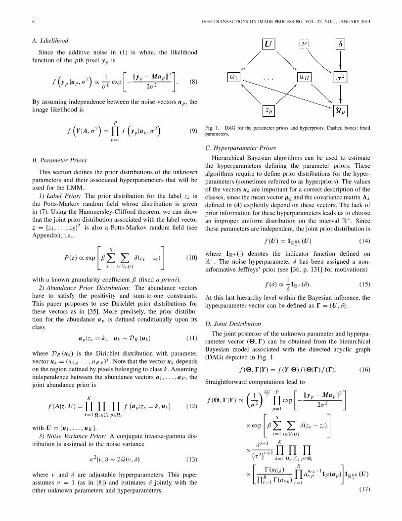
Fig. 1. DAG for the parameter priors and hyperpriors. Dashed boxes: fixedparameters.
C. Hyperparameter Priors
Hierarchical Bayesian algorithms can be used to estimatethe hyperparameters defining the parameter priors. Thesealgorithms require to define prior distributions for the hyper-parameters (sometimes referred to as hyperpriors). The valuesof the vectors uk are important for a correct description of theclasses, since the mean vector μk and the covariance matrix �k
defined in (4) explicitly depend on these vectors. The lack ofprior information for these hyperparameters leads us to choosean improper uniform distribution on the interval R
+. Sincethese parameters are independent, the joint prior distribution is
f (U) = 1R
RK+ (U) (14)
where 1R+(·) denotes the indicator function defined onR
+. The noise hyperparameter δ has been assigned a non-informative Jeffreys’ prior (see [36, p. 131] for motivations)
f (δ) ∝ 1
δ1R+(δ). (15)
At this last hierarchy level within the Bayesian inference, thehyperparameter vector can be defined as � = {U, δ}.
D. Joint Distribution
The joint posterior of the unknown parameter and hyperpa-rameter vector (�,�) can be obtained from the hierarchicalBayesian model associated with the directed acyclic graph(DAG) depicted in Fig. 1
f (�,�|Y) = f (Y |�) f (�|�) f (�). (16)
Straightforward computations lead to
f (�,�|Y) ∝(
1
σ 2
) L P2
P∏
p=1
exp
[
−‖yp − Ma p‖2
2σ 2
]
× exp
⎡
⎣β
S∑
t=1
∑
t∈Vτ (t)
δ(zs − zt )
⎤
⎦
× δν−1
(σ 2)ν+1
K∏
k=1
∏
�s∈Ck
∏
p∈�s
×[
(u0,k)∏R
r=1 (ur,k)
R∏
r=1
aur,k−1r,p 1S (ap)
]
1R
RK+ (U)
(17)
ECHES et al.: ADAPTIVE MRF FOR JOINT UNMIXING AND SEGMENTATION OF HYPERSPECTRAL IMAGES 9
where u0,k = ∑Rr=1 ur,k , (.) is the gamma function and
S is the simplex defined by the sum-to-one and positivityconstraints. This distribution is far too complex to obtainclosed-form expressions for the MMSE or MAP estimatorsof (�,�). Thus, we propose to use MCMC methods forgenerating samples asymptotically distributed according to(17). By excluding the first Nbi generated samples (belongingto the so-called burn in period), it is then possible to approx-imate the MMSE and MAP estimators from the remainingsamples.
IV. HYBRID GIBBS SAMPLER
This section studies a hybrid Metropolis-within-Gibbs sam-pler that iteratively generates samples according to the fullconditional distributions of f (�,�|Y ). The algorithm is sum-marized in Algo. 1 and its main steps will now be detailed.
A. Generating Samples According to P [zs = k|z-s , As , uk]
For a given similarity region �s , Bayes’ theorem yields theconditional distribution of zs
P [zs = k|z-s , As , uk] ∝ f (zs |z-s)∏
p∈�s
f (Ap|zs , uk)
where As is the abundance matrix associated with the pixelsbelonging to the neighborhood �s . Since the label of a givenneighborhood is the same for all pixels, it makes sense thatthe abundance vectors of �s contribute to the conditionaldistribution of zs . The complete expression of the conditionaldistribution is
P [zs = k|z-s, As, uk] ∝ exp
⎡
⎣β∑
t∈Vτ (t)
δ(zs − zt )
⎤
⎦
×∏
p∈�s
(u0,k)∏R
r=1 (ur,k)
R∏
r=1
aur,k−1r,p 1S (a p). (18)
Note that sampling from this conditional distribution canbe achieved by drawing a discrete value in the finite set{1, . . . , K } with the normalized probabilities (18).
B. Generating Samples According to f (a p|zs = k, y p, σ2)
The Bayes’ theorem leads to
f (a p|zs = k, y p, σ2) ∝ f
(a p|zs = k, uk
)f(
yp|a p, σ2)
or equivalently to
f (a p|zs = k, yp, σ2) ∝ exp
[
−‖y p − Map‖2
2σ 2
]
1S(a p)
×R∏
r=1
aur,k−1r,p . (19)
Since it is not easy to sample according to (19), we proposeto use a Metropolis-Hastings step for generating the R − 1first abundance samples and to compute the Rth abundanceusing aR,p = 1 −∑R−1
r=1 ar,p . The proposal distribution for
Algorithm 1 Hybrid Gibbs Sampler for Joint Unmixing andSegmentation
1) % Initialization:1: Generate z(0) by randomly assigning a discrete value
from (1, . . . , K ) to each region �s .2: Generate U(0) and δ(0) from the probability density
functions (pdfs) in (14) and (15).3: Generate A(0) and σ 2(0) from the pdfs in (12) and
(13).2) % Iterations:
1: for t = 1, 2, . . . do2: for each pixel p = 1, . . . , P do3: Sample a(t)
p from the pdf in (19),4: end for5: Sample σ 2(t) from the pdf in (21),6: for each region �s s = 1, . . . , S do7: Sample z(t)
s from the pdf in (18),8: end for9: for each class Ck k = 1, . . . , K do
10: Sample ur,k from the pdf in (22),11: end for12: Sample δ from the pdf in (23),13: end for
this move is a Gaussian distribution with the following meanand covariance matrix (from [8])⎧⎨
⎩
� =[
1σ 2
(M∗ − mR uT
)T (M∗ − mR uT
)]−1,
μ = �[
1σ 2
(M∗ − mR uT
)T (yp − mR
)],
(20)
where M∗ = [m1, . . . , mR−1]
and u = [1, . . . , 1]T ∈ R
R−1.This distribution is truncated on the set defined by the abun-dance constraints (see [37] and [8] for more details).
C. Generating Samples According to f(σ 2|Y , A, δ
)
The conditional distribution of σ 2 is
f (σ 2|Y , A, δ) ∝ f (σ 2|δ)P∏
p=1
f (y p|ap, σ2).
As a consequence, σ 2|Y , A, δ is distributed according to thefollowing inverse-gamma distribution
σ 2|Y , A, δ ∼ IG⎛
⎝ L P
2+1, δ +
P∑
p=1
‖y p − Ma p‖2
2
⎞
⎠. (21)
D. Generating Samples According to f(ur,k |z, ar
)
The Dirichlet parameters are generated for each endmemberr (r = 1, . . . , R) and each class Ck (k = 1, . . . , K )
f(ur,k |z, ar
) ∝ f(ur,k) ∏
�s∈Ck
∏
p∈�s
f(a p|zs = k, uk
)
which leads to
f(ur,k |z, ar
) ∝∏
�s∈Ck
∏
p∈�s
[(u0,k)
(ur,k)a
ur,k−1r,p
]1R+(ur,k).
(22)
10 IEEE TRANSACTIONS ON IMAGE PROCESSING, VOL. 22, NO. 1, JANUARY 2013
Since it is not easy to sample from (22), we propose to use aMetropolis-Hastings move. More precisely, samples are gener-ated using a random-walk defined by the Gaussian distributionN (0, w2), where the variance w2 has been adjusted to obtainan acceptance rate between 0.15 and 0.50 as recommended in[38, p. 55].
E. Generating Samples According to f(δ|σ 2)
The conditional distribution of δ is the following gammadistribution
δ|σ 2∼ G(
1,1
σ 2
)(23)
where G(a, b) is the gamma distribution with shape parametera and scale parameter b [39, p. 581].
V. SIMULATION RESULTS ON SYNTHETIC DATA
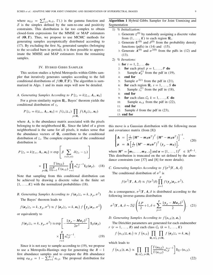
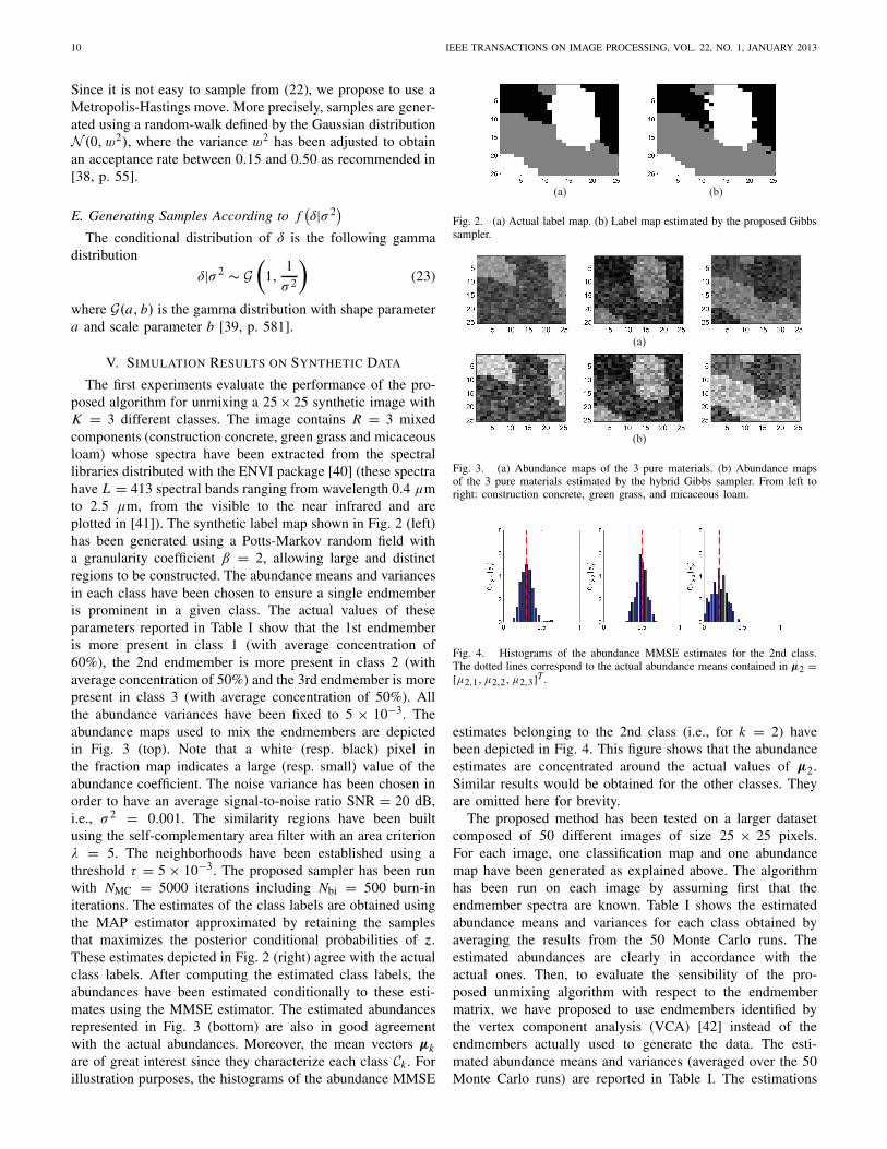
The first experiments evaluate the performance of the pro-posed algorithm for unmixing a 25 × 25 synthetic image withK = 3 different classes. The image contains R = 3 mixedcomponents (construction concrete, green grass and micaceousloam) whose spectra have been extracted from the spectrallibraries distributed with the ENVI package [40] (these spectrahave L = 413 spectral bands ranging from wavelength 0.4 μmto 2.5 μm, from the visible to the near infrared and areplotted in [41]). The synthetic label map shown in Fig. 2 (left)has been generated using a Potts-Markov random field witha granularity coefficient β = 2, allowing large and distinctregions to be constructed. The abundance means and variancesin each class have been chosen to ensure a single endmemberis prominent in a given class. The actual values of theseparameters reported in Table I show that the 1st endmemberis more present in class 1 (with average concentration of60%), the 2nd endmember is more present in class 2 (withaverage concentration of 50%) and the 3rd endmember is morepresent in class 3 (with average concentration of 50%). Allthe abundance variances have been fixed to 5 × 10⁻³. Theabundance maps used to mix the endmembers are depictedin Fig. 3 (top). Note that a white (resp. black) pixel inthe fraction map indicates a large (resp. small) value of theabundance coefficient. The noise variance has been chosen inorder to have an average signal-to-noise ratio SNR = 20 dB,i.e., σ 2 = 0.001. The similarity regions have been builtusing the self-complementary area filter with an area criterionλ = 5. The neighborhoods have been established using athreshold τ = 5 × 10⁻³. The proposed sampler has been runwith NMC = 5000 iterations including Nbi = 500 burn-initerations. The estimates of the class labels are obtained usingthe MAP estimator approximated by retaining the samplesthat maximizes the posterior conditional probabilities of z.These estimates depicted in Fig. 2 (right) agree with the actualclass labels. After computing the estimated class labels, theabundances have been estimated conditionally to these esti-mates using the MMSE estimator. The estimated abundancesrepresented in Fig. 3 (bottom) are also in good agreementwith the actual abundances. Moreover, the mean vectors μkare of great interest since they characterize each class Ck . Forillustration purposes, the histograms of the abundance MMSE
(a) (b)
Fig. 2. (a) Actual label map. (b) Label map estimated by the proposed Gibbssampler.
(a)
(b)
Fig. 3. (a) Abundance maps of the 3 pure materials. (b) Abundance mapsof the 3 pure materials estimated by the hybrid Gibbs sampler. From left toright: construction concrete, green grass, and micaceous loam.
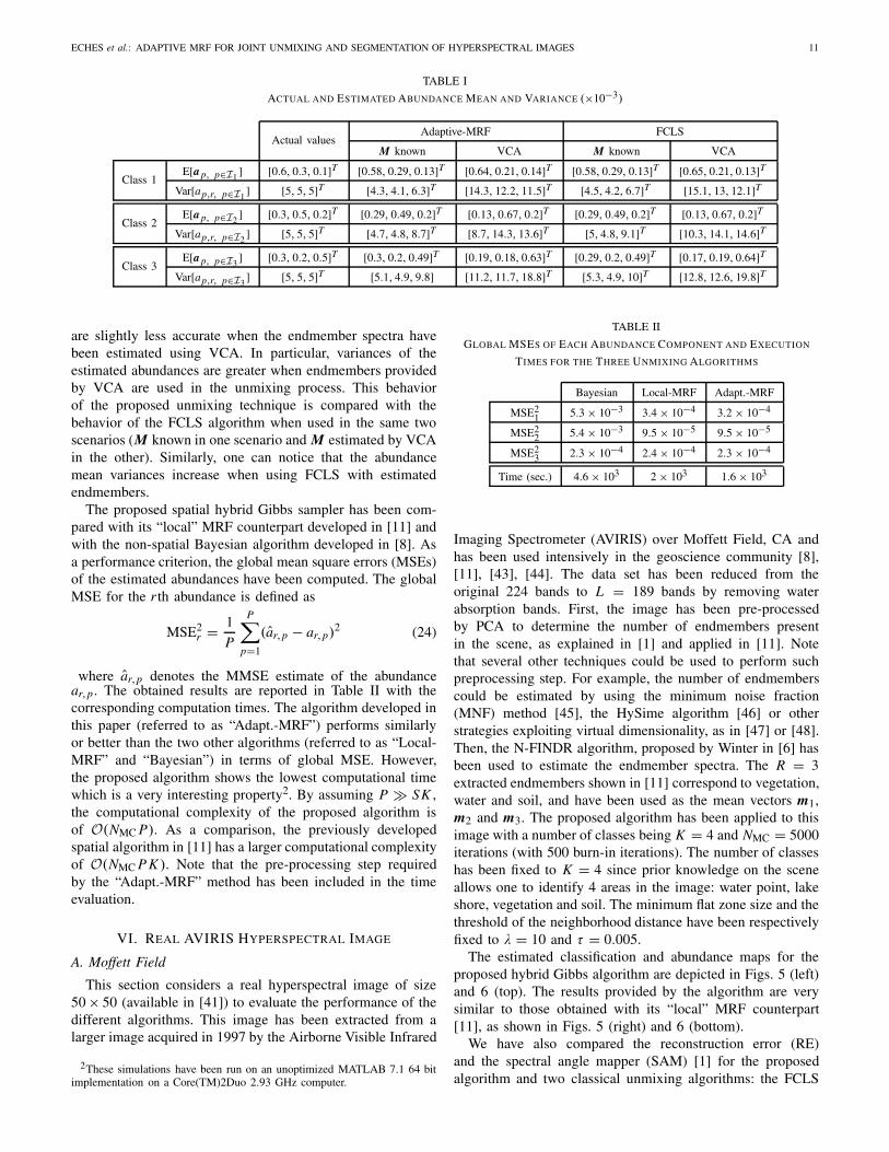
Fig. 4. Histograms of the abundance MMSE estimates for the 2nd class.The dotted lines correspond to the actual abundance means contained in μ2 =[μ2,1, μ2,2, μ2,3]T.
estimates belonging to the 2nd class (i.e., for k = 2) havebeen depicted in Fig. 4. This figure shows that the abundanceestimates are concentrated around the actual values of μ2.Similar results would be obtained for the other classes. Theyare omitted here for brevity.
The proposed method has been tested on a larger datasetcomposed of 50 different images of size 25 × 25 pixels.For each image, one classification map and one abundancemap have been generated as explained above. The algorithmhas been run on each image by assuming first that theendmember spectra are known. Table I shows the estimatedabundance means and variances for each class obtained byaveraging the results from the 50 Monte Carlo runs. Theestimated abundances are clearly in accordance with theactual ones. Then, to evaluate the sensibility of the pro-posed unmixing algorithm with respect to the endmembermatrix, we have proposed to use endmembers identified bythe vertex component analysis (VCA) [42] instead of theendmembers actually used to generate the data. The esti-mated abundance means and variances (averaged over the 50Monte Carlo runs) are reported in Table I. The estimations
ECHES et al.: ADAPTIVE MRF FOR JOINT UNMIXING AND SEGMENTATION OF HYPERSPECTRAL IMAGES 11
TABLE I
ACTUAL AND ESTIMATED ABUNDANCE MEAN AND VARIANCE (×10−3)
Actual valuesAdaptive-MRF FCLS
M known VCA M known VCA
Class 1E[a p, p∈I1 ] [0.6, 0.3, 0.1]T [0.58, 0.29, 0.13]T [0.64, 0.21, 0.14]T [0.58, 0.29, 0.13]T [0.65, 0.21, 0.13]T
Var[ap,r, p∈I1 ] [5, 5, 5]T [4.3, 4.1, 6.3]T [14.3, 12.2, 11.5]T [4.5, 4.2, 6.7]T [15.1, 13, 12.1]T
Class 2E[a p, p∈I2 ] [0.3, 0.5, 0.2]T [0.29, 0.49, 0.2]T [0.13, 0.67, 0.2]T [0.29, 0.49, 0.2]T [0.13, 0.67, 0.2]T
Var[ap,r, p∈I2 ] [5, 5, 5]T [4.7, 4.8, 8.7]T [8.7, 14.3, 13.6]T [5, 4.8, 9.1]T [10.3, 14.1, 14.6]T
Class 3E[a p, p∈I3
] [0.3, 0.2, 0.5]T [0.3, 0.2, 0.49]T [0.19, 0.18, 0.63]T [0.29, 0.2, 0.49]T [0.17, 0.19, 0.64]TVar[ap,r, p∈I3
] [5, 5, 5]T [5.1, 4.9, 9.8] [11.2, 11.7, 18.8]T [5.3, 4.9, 10]T [12.8, 12.6, 19.8]T
are slightly less accurate when the endmember spectra havebeen estimated using VCA. In particular, variances of theestimated abundances are greater when endmembers providedby VCA are used in the unmixing process. This behaviorof the proposed unmixing technique is compared with thebehavior of the FCLS algorithm when used in the same twoscenarios (M known in one scenario and M estimated by VCAin the other). Similarly, one can notice that the abundancemean variances increase when using FCLS with estimatedendmembers.
The proposed spatial hybrid Gibbs sampler has been com-pared with its “local” MRF counterpart developed in [11] andwith the non-spatial Bayesian algorithm developed in [8]. Asa performance criterion, the global mean square errors (MSEs)of the estimated abundances have been computed. The globalMSE for the r th abundance is defined as
MSE2r = 1
P
P∑
p=1
(ar,p − ar,p)2 (24)
where ar,p denotes the MMSE estimate of the abundancear,p . The obtained results are reported in Table II with thecorresponding computation times. The algorithm developed inthis paper (referred to as “Adapt.-MRF”) performs similarlyor better than the two other algorithms (referred to as “Local-MRF” and “Bayesian”) in terms of global MSE. However,the proposed algorithm shows the lowest computational timewhich is a very interesting property2. By assuming P � SK ,the computational complexity of the proposed algorithm isof O(NMC P). As a comparison, the previously developedspatial algorithm in [11] has a larger computational complexityof O(NMC P K ). Note that the pre-processing step requiredby the “Adapt.-MRF” method has been included in the timeevaluation.
VI. REAL AVIRIS HYPERSPECTRAL IMAGE
A. Moffett Field
This section considers a real hyperspectral image of size50 × 50 (available in [41]) to evaluate the performance of thedifferent algorithms. This image has been extracted from alarger image acquired in 1997 by the Airborne Visible Infrared
2These simulations have been run on an unoptimized MATLAB 7.1 64 bitimplementation on a Core(TM)2Duo 2.93 GHz computer.
TABLE II
GLOBAL MSES OF EACH ABUNDANCE COMPONENT AND EXECUTION
TIMES FOR THE THREE UNMIXING ALGORITHMS
Bayesian Local-MRF Adapt.-MRF
MSE21 5.3 × 10⁻³ 3.4 × 10⁻⁴ 3.2 × 10⁻⁴
MSE22 5.4 × 10⁻³ 9.5 × 10⁻⁵ 9.5 × 10⁻⁵
MSE23 2.3 × 10⁻⁴ 2.4 × 10⁻⁴ 2.3 × 10⁻⁴
Time (sec.) 4.6 × 10³ 2 × 10³ 1.6 × 10³
Imaging Spectrometer (AVIRIS) over Moffett Field, CA andhas been used intensively in the geoscience community [8],[11], [43], [44]. The data set has been reduced from theoriginal 224 bands to L = 189 bands by removing waterabsorption bands. First, the image has been pre-processedby PCA to determine the number of endmembers presentin the scene, as explained in [1] and applied in [11]. Notethat several other techniques could be used to perform suchpreprocessing step. For example, the number of endmemberscould be estimated by using the minimum noise fraction(MNF) method [45], the HySime algorithm [46] or otherstrategies exploiting virtual dimensionality, as in [47] or [48].Then, the N-FINDR algorithm, proposed by Winter in [6] hasbeen used to estimate the endmember spectra. The R = 3extracted endmembers shown in [11] correspond to vegetation,water and soil, and have been used as the mean vectors m1,m2 and m3. The proposed algorithm has been applied to thisimage with a number of classes being K = 4 and NMC = 5000iterations (with 500 burn-in iterations). The number of classeshas been fixed to K = 4 since prior knowledge on the sceneallows one to identify 4 areas in the image: water point, lakeshore, vegetation and soil. The minimum flat zone size and thethreshold of the neighborhood distance have been respectivelyfixed to λ = 10 and τ = 0.005.
The estimated classification and abundance maps for theproposed hybrid Gibbs algorithm are depicted in Figs. 5 (left)and 6 (top). The results provided by the algorithm are verysimilar to those obtained with its “local” MRF counterpart[11], as shown in Figs. 5 (right) and 6 (bottom).
We have also compared the reconstruction error (RE)and the spectral angle mapper (SAM) [1] for the proposedalgorithm and two classical unmixing algorithms: the FCLS
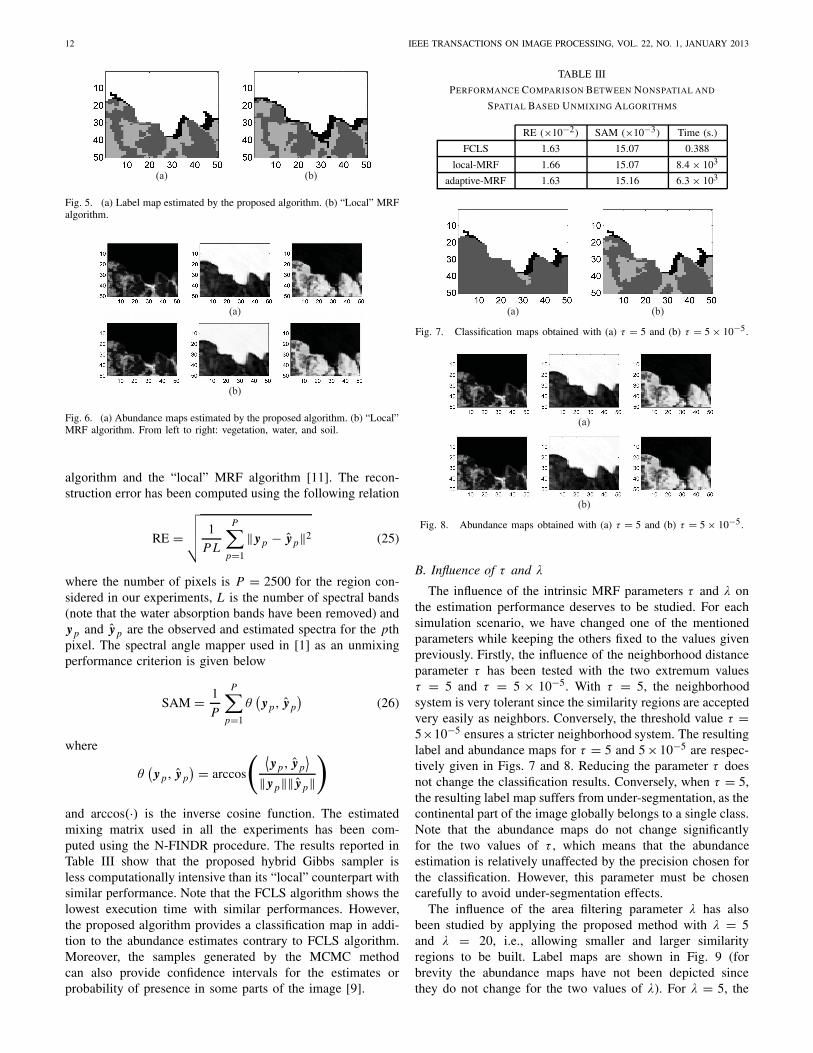
12 IEEE TRANSACTIONS ON IMAGE PROCESSING, VOL. 22, NO. 1, JANUARY 2013
(a) (b)
Fig. 5. (a) Label map estimated by the proposed algorithm. (b) “Local” MRFalgorithm.
(a)
(b)
Fig. 6. (a) Abundance maps estimated by the proposed algorithm. (b) “Local”MRF algorithm. From left to right: vegetation, water, and soil.
algorithm and the “local” MRF algorithm [11]. The recon-struction error has been computed using the following relation
RE =√√√√ 1
P L
P∑
p=1
‖y p − yp‖2 (25)
where the number of pixels is P = 2500 for the region con-sidered in our experiments, L is the number of spectral bands(note that the water absorption bands have been removed) andyp and y p are the observed and estimated spectra for the pthpixel. The spectral angle mapper used in [1] as an unmixingperformance criterion is given below
SAM = 1
P
P∑
p=1
θ(
yp, y p
)(26)
where
θ(
yp, y p) = arccos
( ⟨y p, yp
⟩
‖y p‖‖ y p‖
)
and arccos(·) is the inverse cosine function. The estimatedmixing matrix used in all the experiments has been com-puted using the N-FINDR procedure. The results reported inTable III show that the proposed hybrid Gibbs sampler isless computationally intensive than its “local” counterpart withsimilar performance. Note that the FCLS algorithm shows thelowest execution time with similar performances. However,the proposed algorithm provides a classification map in addi-tion to the abundance estimates contrary to FCLS algorithm.Moreover, the samples generated by the MCMC methodcan also provide confidence intervals for the estimates orprobability of presence in some parts of the image [9].
TABLE III
PERFORMANCE COMPARISON BETWEEN NONSPATIAL AND
SPATIAL BASED UNMIXING ALGORITHMS
RE (×10−2) SAM (×10−3) Time (s.)
FCLS 1.63 15.07 0.388
local-MRF 1.66 15.07 8.4 × 10³
adaptive-MRF 1.63 15.16 6.3 × 10³
(a) (b)
Fig. 7. Classification maps obtained with (a) τ = 5 and (b) τ = 5 × 10⁻⁵.
(a)
(b)
Fig. 8. Abundance maps obtained with (a) τ = 5 and (b) τ = 5 × 10⁻⁵.
B. Influence of τ and λ
The influence of the intrinsic MRF parameters τ and λ onthe estimation performance deserves to be studied. For eachsimulation scenario, we have changed one of the mentionedparameters while keeping the others fixed to the values givenpreviously. Firstly, the influence of the neighborhood distanceparameter τ has been tested with the two extremum valuesτ = 5 and τ = 5 × 10⁻⁵. With τ = 5, the neighborhoodsystem is very tolerant since the similarity regions are acceptedvery easily as neighbors. Conversely, the threshold value τ =5×10⁻⁵ ensures a stricter neighborhood system. The resultinglabel and abundance maps for τ = 5 and 5 ×10⁻⁵ are respec-tively given in Figs. 7 and 8. Reducing the parameter τ doesnot change the classification results. Conversely, when τ = 5,the resulting label map suffers from under-segmentation, as thecontinental part of the image globally belongs to a single class.Note that the abundance maps do not change significantlyfor the two values of τ , which means that the abundanceestimation is relatively unaffected by the precision chosen forthe classification. However, this parameter must be chosencarefully to avoid under-segmentation effects.
The influence of the area filtering parameter λ has alsobeen studied by applying the proposed method with λ = 5and λ = 20, i.e., allowing smaller and larger similarityregions to be built. Label maps are shown in Fig. 9 (forbrevity the abundance maps have not been depicted sincethey do not change for the two values of λ). For λ = 5, the
ECHES et al.: ADAPTIVE MRF FOR JOINT UNMIXING AND SEGMENTATION OF HYPERSPECTRAL IMAGES 13
(a) (b)
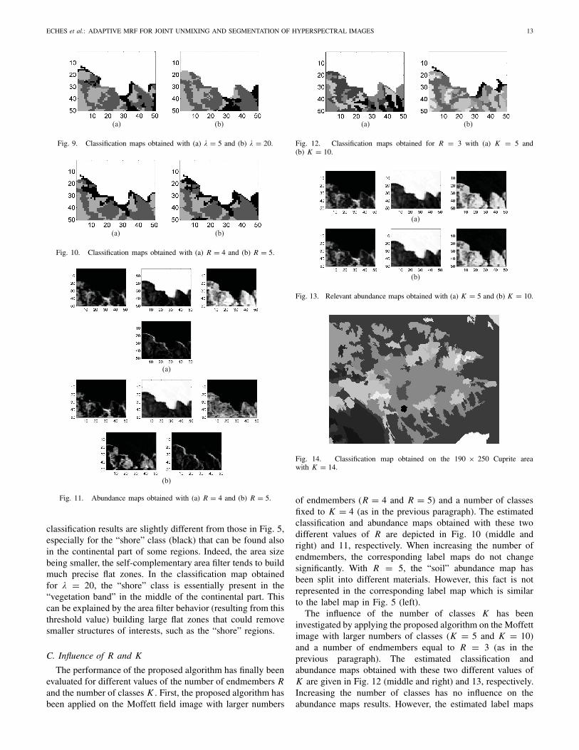
Fig. 9. Classification maps obtained with (a) λ = 5 and (b) λ = 20.
(a) (b)
Fig. 10. Classification maps obtained with (a) R = 4 and (b) R = 5.
(a)
(b)
Fig. 11. Abundance maps obtained with (a) R = 4 and (b) R = 5.
classification results are slightly different from those in Fig. 5,especially for the “shore” class (black) that can be found alsoin the continental part of some regions. Indeed, the area sizebeing smaller, the self-complementary area filter tends to buildmuch precise flat zones. In the classification map obtainedfor λ = 20, the “shore” class is essentially present in the“vegetation band” in the middle of the continental part. Thiscan be explained by the area filter behavior (resulting from thisthreshold value) building large flat zones that could removesmaller structures of interests, such as the “shore” regions.
C. Influence of R and K
The performance of the proposed algorithm has finally beenevaluated for different values of the number of endmembers Rand the number of classes K . First, the proposed algorithm hasbeen applied on the Moffett field image with larger numbers
(a) (b)
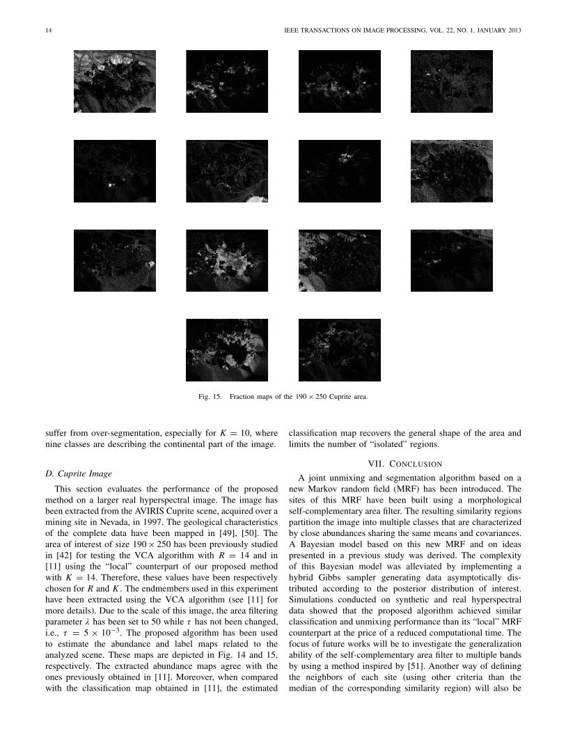
Fig. 12. Classification maps obtained for R = 3 with (a) K = 5 and(b) K = 10.
(a)
(b)
Fig. 13. Relevant abundance maps obtained with (a) K = 5 and (b) K = 10.
Fig. 14. Classification map obtained on the 190 × 250 Cuprite areawith K = 14.
of endmembers (R = 4 and R = 5) and a number of classesfixed to K = 4 (as in the previous paragraph). The estimatedclassification and abundance maps obtained with these twodifferent values of R are depicted in Fig. 10 (middle andright) and 11, respectively. When increasing the number ofendmembers, the corresponding label maps do not changesignificantly. With R = 5, the “soil” abundance map hasbeen split into different materials. However, this fact is notrepresented in the corresponding label map which is similarto the label map in Fig. 5 (left).
The influence of the number of classes K has beeninvestigated by applying the proposed algorithm on the Moffettimage with larger numbers of classes (K = 5 and K = 10)and a number of endmembers equal to R = 3 (as in theprevious paragraph). The estimated classification andabundance maps obtained with these two different values ofK are given in Fig. 12 (middle and right) and 13, respectively.Increasing the number of classes has no influence on theabundance maps results. However, the estimated label maps
14 IEEE TRANSACTIONS ON IMAGE PROCESSING, VOL. 22, NO. 1, JANUARY 2013
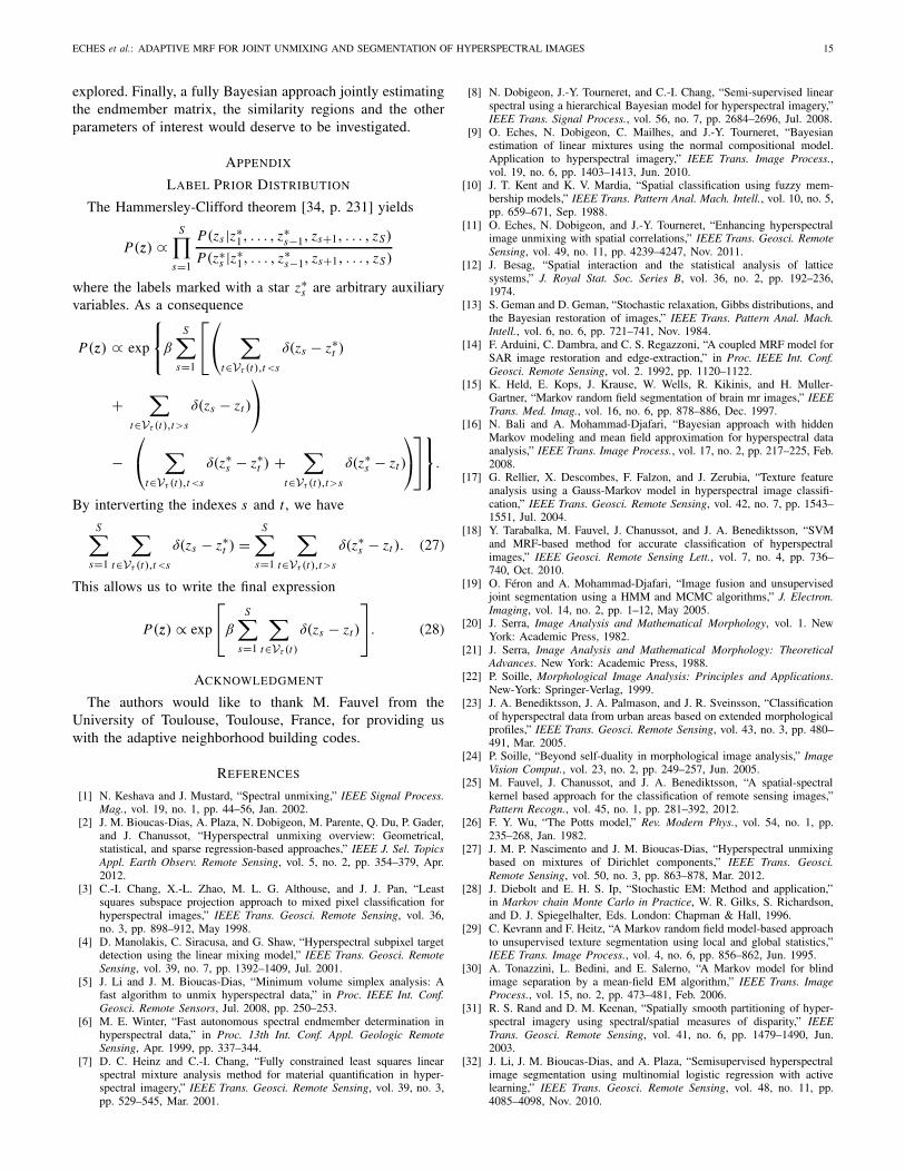
Fig. 15. Fraction maps of the 190 × 250 Cuprite area.
suffer from over-segmentation, especially for K = 10, wherenine classes are describing the continental part of the image.
D. Cuprite Image
This section evaluates the performance of the proposedmethod on a larger real hyperspectral image. The image hasbeen extracted from the AVIRIS Cuprite scene, acquired over amining site in Nevada, in 1997. The geological characteristicsof the complete data have been mapped in [49], [50]. Thearea of interest of size 190 × 250 has been previously studiedin [42] for testing the VCA algorithm with R = 14 and in[11] using the “local” counterpart of our proposed methodwith K = 14. Therefore, these values have been respectivelychosen for R and K . The endmembers used in this experimenthave been extracted using the VCA algorithm (see [11] formore details). Due to the scale of this image, the area filteringparameter λ has been set to 50 while τ has not been changed,i.e., τ = 5 × 10⁻³. The proposed algorithm has been usedto estimate the abundance and label maps related to theanalyzed scene. These maps are depicted in Fig. 14 and 15,respectively. The extracted abundance maps agree with theones previously obtained in [11]. Moreover, when comparedwith the classification map obtained in [11], the estimated
classification map recovers the general shape of the area andlimits the number of “isolated” regions.
VII. CONCLUSION
A joint unmixing and segmentation algorithm based on anew Markov random field (MRF) has been introduced. Thesites of this MRF have been built using a morphologicalself-complementary area filter. The resulting similarity regionspartition the image into multiple classes that are characterizedby close abundances sharing the same means and covariances.A Bayesian model based on this new MRF and on ideaspresented in a previous study was derived. The complexityof this Bayesian model was alleviated by implementing ahybrid Gibbs sampler generating data asymptotically dis-tributed according to the posterior distribution of interest.Simulations conducted on synthetic and real hyperspectraldata showed that the proposed algorithm achieved similarclassification and unmixing performance than its “local” MRFcounterpart at the price of a reduced computational time. Thefocus of future works will be to investigate the generalizationability of the self-complementary area filter to multiple bandsby using a method inspired by [51]. Another way of definingthe neighbors of each site (using other criteria than themedian of the corresponding similarity region) will also be
ECHES et al.: ADAPTIVE MRF FOR JOINT UNMIXING AND SEGMENTATION OF HYPERSPECTRAL IMAGES 15
explored. Finally, a fully Bayesian approach jointly estimatingthe endmember matrix, the similarity regions and the otherparameters of interest would deserve to be investigated.
APPENDIX
LABEL PRIOR DISTRIBUTION
The Hammersley-Clifford theorem [34, p. 231] yields
P(z) ∝S∏
s=1
P(zs |z∗1, . . . , z∗
s−1, zs+1, . . . , zS)
P(z∗s |z∗
1, . . . , z∗s−1, zs+1, . . . , zS)
where the labels marked with a star z∗s are arbitrary auxiliary
variables. As a consequence
P(z) ∝ exp
⎧⎨
⎩β
S∑
s=1
⎡
⎣
⎛
⎝∑
t∈Vτ (t),t<s
δ(zs − z∗t )
+∑
t∈Vτ (t),t>s
δ(zs − zt )
⎞
⎠
−⎛
⎝∑
t∈Vτ (t),t<s
δ(z∗s − z∗
t ) +∑
t∈Vτ (t),t>s
δ(z∗s − zt )
⎞
⎠
⎤
⎦
⎫⎬
⎭.
By interverting the indexes s and t , we have
S∑
s=1
∑
t∈Vτ (t),t<s
δ(zs − z∗t ) =
S∑
s=1
∑
t∈Vτ (t),t>s
δ(z∗s − zt ). (27)
This allows us to write the final expression
P(z) ∝ exp
⎡
⎣β
S∑
s=1
∑
t∈Vτ (t)
δ(zs − zt )
⎤
⎦. (28)
ACKNOWLEDGMENT
The authors would like to thank M. Fauvel from theUniversity of Toulouse, Toulouse, France, for providing uswith the adaptive neighborhood building codes.
REFERENCES
[1] N. Keshava and J. Mustard, “Spectral unmixing,” IEEE Signal Process.Mag., vol. 19, no. 1, pp. 44–56, Jan. 2002.
[2] J. M. Bioucas-Dias, A. Plaza, N. Dobigeon, M. Parente, Q. Du, P. Gader,and J. Chanussot, “Hyperspectral unmixing overview: Geometrical,statistical, and sparse regression-based approaches,” IEEE J. Sel. TopicsAppl. Earth Observ. Remote Sensing, vol. 5, no. 2, pp. 354–379, Apr.2012.
[3] C.-I. Chang, X.-L. Zhao, M. L. G. Althouse, and J. J. Pan, “Leastsquares subspace projection approach to mixed pixel classification forhyperspectral images,” IEEE Trans. Geosci. Remote Sensing, vol. 36,no. 3, pp. 898–912, May 1998.
[4] D. Manolakis, C. Siracusa, and G. Shaw, “Hyperspectral subpixel targetdetection using the linear mixing model,” IEEE Trans. Geosci. RemoteSensing, vol. 39, no. 7, pp. 1392–1409, Jul. 2001.
[5] J. Li and J. M. Bioucas-Dias, “Minimum volume simplex analysis: Afast algorithm to unmix hyperspectral data,” in Proc. IEEE Int. Conf.Geosci. Remote Sensors, Jul. 2008, pp. 250–253.
[6] M. E. Winter, “Fast autonomous spectral endmember determination inhyperspectral data,” in Proc. 13th Int. Conf. Appl. Geologic RemoteSensing, Apr. 1999, pp. 337–344.
[7] D. C. Heinz and C.-I. Chang, “Fully constrained least squares linearspectral mixture analysis method for material quantification in hyper-spectral imagery,” IEEE Trans. Geosci. Remote Sensing, vol. 39, no. 3,pp. 529–545, Mar. 2001.
[8] N. Dobigeon, J.-Y. Tourneret, and C.-I. Chang, “Semi-supervised linearspectral using a hierarchical Bayesian model for hyperspectral imagery,”IEEE Trans. Signal Process., vol. 56, no. 7, pp. 2684–2696, Jul. 2008.
[9] O. Eches, N. Dobigeon, C. Mailhes, and J.-Y. Tourneret, “Bayesianestimation of linear mixtures using the normal compositional model.Application to hyperspectral imagery,” IEEE Trans. Image Process.,vol. 19, no. 6, pp. 1403–1413, Jun. 2010.
[10] J. T. Kent and K. V. Mardia, “Spatial classification using fuzzy mem-bership models,” IEEE Trans. Pattern Anal. Mach. Intell., vol. 10, no. 5,pp. 659–671, Sep. 1988.
[11] O. Eches, N. Dobigeon, and J.-Y. Tourneret, “Enhancing hyperspectralimage unmixing with spatial correlations,” IEEE Trans. Geosci. RemoteSensing, vol. 49, no. 11, pp. 4239–4247, Nov. 2011.
[12] J. Besag, “Spatial interaction and the statistical analysis of latticesystems,” J. Royal Stat. Soc. Series B, vol. 36, no. 2, pp. 192–236,1974.
[13] S. Geman and D. Geman, “Stochastic relaxation, Gibbs distributions, andthe Bayesian restoration of images,” IEEE Trans. Pattern Anal. Mach.Intell., vol. 6, no. 6, pp. 721–741, Nov. 1984.
[14] F. Arduini, C. Dambra, and C. S. Regazzoni, “A coupled MRF model forSAR image restoration and edge-extraction,” in Proc. IEEE Int. Conf.Geosci. Remote Sensing, vol. 2. 1992, pp. 1120–1122.
[15] K. Held, E. Kops, J. Krause, W. Wells, R. Kikinis, and H. Muller-Gartner, “Markov random field segmentation of brain mr images,” IEEETrans. Med. Imag., vol. 16, no. 6, pp. 878–886, Dec. 1997.
[16] N. Bali and A. Mohammad-Djafari, “Bayesian approach with hiddenMarkov modeling and mean field approximation for hyperspectral dataanalysis,” IEEE Trans. Image Process., vol. 17, no. 2, pp. 217–225, Feb.2008.
[17] G. Rellier, X. Descombes, F. Falzon, and J. Zerubia, “Texture featureanalysis using a Gauss-Markov model in hyperspectral image classifi-cation,” IEEE Trans. Geosci. Remote Sensing, vol. 42, no. 7, pp. 1543–1551, Jul. 2004.
[18] Y. Tarabalka, M. Fauvel, J. Chanussot, and J. A. Benediktsson, “SVMand MRF-based method for accurate classification of hyperspectralimages,” IEEE Geosci. Remote Sensing Lett., vol. 7, no. 4, pp. 736–740, Oct. 2010.
[19] O. Féron and A. Mohammad-Djafari, “Image fusion and unsupervisedjoint segmentation using a HMM and MCMC algorithms,” J. Electron.Imaging, vol. 14, no. 2, pp. 1–12, May 2005.
[20] J. Serra, Image Analysis and Mathematical Morphology, vol. 1. NewYork: Academic Press, 1982.
[21] J. Serra, Image Analysis and Mathematical Morphology: TheoreticalAdvances. New York: Academic Press, 1988.
[22] P. Soille, Morphological Image Analysis: Principles and Applications.New-York: Springer-Verlag, 1999.
[23] J. A. Benediktsson, J. A. Palmason, and J. R. Sveinsson, “Classificationof hyperspectral data from urban areas based on extended morphologicalprofiles,” IEEE Trans. Geosci. Remote Sensing, vol. 43, no. 3, pp. 480–491, Mar. 2005.
[24] P. Soille, “Beyond self-duality in morphological image analysis,” ImageVision Comput., vol. 23, no. 2, pp. 249–257, Jun. 2005.
[25] M. Fauvel, J. Chanussot, and J. A. Benediktsson, “A spatial-spectralkernel based approach for the classification of remote sensing images,”Pattern Recogn., vol. 45, no. 1, pp. 281–392, 2012.
[26] F. Y. Wu, “The Potts model,” Rev. Modern Phys., vol. 54, no. 1, pp.235–268, Jan. 1982.
[27] J. M. P. Nascimento and J. M. Bioucas-Dias, “Hyperspectral unmixingbased on mixtures of Dirichlet components,” IEEE Trans. Geosci.Remote Sensing, vol. 50, no. 3, pp. 863–878, Mar. 2012.
[28] J. Diebolt and E. H. S. Ip, “Stochastic EM: Method and application,”in Markov chain Monte Carlo in Practice, W. R. Gilks, S. Richardson,and D. J. Spiegelhalter, Eds. London: Chapman & Hall, 1996.
[29] C. Kevrann and F. Heitz, “A Markov random field model-based approachto unsupervised texture segmentation using local and global statistics,”IEEE Trans. Image Process., vol. 4, no. 6, pp. 856–862, Jun. 1995.
[30] A. Tonazzini, L. Bedini, and E. Salerno, “A Markov model for blindimage separation by a mean-field EM algorithm,” IEEE Trans. ImageProcess., vol. 15, no. 2, pp. 473–481, Feb. 2006.
[31] R. S. Rand and D. M. Keenan, “Spatially smooth partitioning of hyper-spectral imagery using spectral/spatial measures of disparity,” IEEETrans. Geosci. Remote Sensing, vol. 41, no. 6, pp. 1479–1490, Jun.2003.
[32] J. Li, J. M. Bioucas-Dias, and A. Plaza, “Semisupervised hyperspectralimage segmentation using multinomial logistic regression with activelearning,” IEEE Trans. Geosci. Remote Sensing, vol. 48, no. 11, pp.4085–4098, Nov. 2010.
16 IEEE TRANSACTIONS ON IMAGE PROCESSING, VOL. 22, NO. 1, JANUARY 2013
[33] B. D. Ripley, Statistical Inference for Spatial Processes. Cambridge,U.K.: Cambridge Univ. Press, 1988.
[34] J.-M. Marin and C. P. Robert, Bayesian Core: A Practical Approach toComputational Bayesian Statistics. New-York: Springer-Verlag, 2007.
[35] R. Mittelman, N. Dobigeon, and A. O. Hero, “Hyperspectral imageunmixing using a multiresolution sticky HDP,” IEEE Signal Process.,vol. 60, no. 4, pp. 1656–1671, Apr. 2012.
[36] C. P. Robert, The Bayesian Choice: From Decision-Theoretic Moti-vations to Computational Implementation. New York: Springer-Verlag,2007.
[37] N. Dobigeon and J.-Y. Tourneret. (2007, Mar.). Efficient SamplingAccording to a Multivariate Gaussian Distribution Truncated on aSimplex. IRIT/ENSEEIHT/TeSA, Toulouse, France [Online]. Available:http:// dobigeon.perso.enseeiht.fr/ papers/ Dobigeon _TechReport_2007b.pdf
[38] G. O. Roberts, “Markov chain concepts related to sampling algorithms,”in Markov Chain Monte Carlo in Practice, W. R. Gilks, S. Richardson,and D. J. Spiegelhalter, Eds. London: Chapman & Hall, 1996, pp. 45–57.
[39] C. P. Robert and G. Casella, Monte Carlo Statistical Methods. NewYork: Springer-Verlag, 2004.
[40] ENVI Users Guide Version 4.0, Research Systems Inc., Boulder, CO,Sep. 2003.
[41] O. Eches, N. Dobigeon, and J.-Y. Tourneret, “Estimating the numberof endmembers in hyperspectral images using the normal compositionalmodel and a hierarchical Bayesian algorithm,” IEEE J. Sel. Topics SignalProcess., vol. 3, no. 3, pp. 582–591, Jun. 2010.
[42] J. M. P. Nascimento and J. M. Bioucas-Dias, “Vertex componentanalysis: A fast algorithm to unmix hyperspectral data,” IEEE Trans.Geosci. Remote Sensing, vol. 43, no. 4, pp. 898–910, Apr. 2005.
[43] E. Christophe, D. Léger, and C. Mailhes, “Quality criteria benchmark forhyperspectral imagery,” IEEE Trans. Geosci. Remote Sensing, vol. 43,no. 9, pp. 2103–2114, Sep. 2005.
[44] T. Akgun, Y. Altunbasak, and R. M. Mersereau, “Super-resolutionreconstruction of hyperspectral images,” IEEE Trans. Image Process.,vol. 14, no. 11, pp. 1860–1875, Nov. 2005.
[45] A. Green, M. Berman, P. Switzer, and M. D. Craig, “A transformation forordering multispectral data in terms of image quality with implicationsfor noise removal,” IEEE Trans. Geosci. Remote Sensing, vol. 26, no. 1,pp. 65–74, Jan. 1994.
[46] J. M. Bioucas-Dias and J. M. P. Nascimento, “Hyperspectral subspaceidentification,” IEEE Trans. Geosci. Remote Sensing, vol. 46, no. 8, pp.2435–2445, Aug. 2008.
[47] C.-I. Chang and Q. Du, “Estimation of number of spectrally distinctsignal sources in hyperspectral imagery,” IEEE Trans. Geosci. RemoteSensing, vol. 42, no. 3, pp. 608–619, Mar. 2004.
[48] B. Luo, J. Chanussot, S. Douté, and X. Ceamanos, “Empirical automaticestimation of the number of endmembers in hyperspectral images,” IEEEGeosci. Remote Sensing Lett., no. 99, 2012, to be published.
[49] R. N. Clark, G. A. Swayze, and A. Gallagher, “Mapping minerals withimaging spectroscopy, U.S. Geological Survey,” Off. Mineral Resour.Bullet., vol. 2039, pp. 141–150, 1993.
[50] R. N. Clark, G. A. Swayze, K. E. Livo, R. F. Kokaly, S. J. Sutley, J. B.Dalton, R. R. McDougal, and C. A. Gent, “Imaging spectroscopy: Earthand planetary remote sensing with the USGS Tetracorder and expertsystems,” J. Geophys. Res., vol. 108, no. E12, pp. 1–44, Dec. 2003.
[51] S. Velasco-Forero and J. Angulo, “Supervised ordering in R p : Applica-tion to morphological processing of hyperspectral images,” IEEE Trans.Image Process., vol. 20, no. 11, pp. 3301–3308, Nov. 2011.
Olivier Eches was born in Villefranche-de-Rouergue, France, in 1984. He received theEng. degree in electrical engineering fromÉcole Nationale Supérieure d’Électronique,d’Électrotechnique, d’Informatique et d’Hydrauliquein Toulouse (ENSEEIHT), Toulouse, France, in2007, and the M.Sc. and Ph.D. degrees in signalprocessing from the National Polytechnic Instituteof Toulouse, the University of Toulouse, in 2007and 2010, respectively.
From 2010 to 2011, he was a PostdoctoralResearch Associate with the Department of Electrical and ComputerEngineering, University of Iceland, Reykjavik, Iceland, working on jointsegmentation and unmixing of hyperspectral images. He is currently aPost-Doctoral Research Associate with the Institut Fresnel, Marseille, France.His current research interests include unmixing sea bottom using nonnegativematrix factorization methods.
Jón Atli Benediktsson (S’84–M’90–SM’99–F’04)received the Cand.Sci. degree in electrical engi-neering from the University of Iceland, Reykjavik,Iceland, in 1984, and the M.S.E.E. and Ph.D. degreesfrom Purdue University, West Lafayette, IN, in 1987and 1990, respectively.
He is currently Pro Rector for Academic Affairsand Professor of Electrical and Computer Engi-neering at the University of Iceland. His researchinterests are in remote sensing, biomedical analysisof signals, pattern recognition, image processing,
and signal processing, and he has published extensively in those fields.Prof. Benediktsson is the President of the IEEE Geoscience and Remote
Sensing Society (GRSS) from 2011 to 2012 and has been on the GRSSAdCom since 1999. He was an Editor of the IEEE TRANSACTIONS ONGEOSCIENCE AND REMOTE SENSING (TGRS) from 2003 to 2008, andhas served as an Associate Editor of TGRS since 1999 and the IEEEGEOSCIENCE AND REMOTE SENSING LETTERS since 2003. He is a co-founder of the biomedical startup company Oxymap. He was a recipient ofthe Stevan J. Kristof Award from Purdue University in 1991 as OutstandingGraduate Student in remote sensing. He was the recipient of the OutstandingYoung Researcher Award by Icelandic Research Council in 1997. He wasgranted the IEEE Third Millennium Medal in 2000. He was a co-recipientof the Technology Innovation Award by the University of Iceland in 2004.He was a recipient of the Yearly Research Award from the EngineeringResearch Institute of the University of Iceland in 2006, and he was a recipientof the Outstanding Service Award from the IEEE Geoscience and RemoteSensing Society in 2007. He is a co-recipient of the IEEE TRANSACTIONS
ON GEOSCIENCE AND REMOTE SENSING Best Paper Award in 2012. He isa member of Societas Scinetiarum Islandica and Tau Beta Pi.
Nicolas Dobigeon (S’05–M’08) was born inAngoulême, France, in 1981. He received the Eng.degree in electrical engineering from ENSEEIHT,Toulouse, France, in 2004, and the M.Sc. and Ph.D.degrees in signal processing from the National Poly-technic Institute of Toulouse, in 2004 and 2007,respectively.
From 2007 to 2008, he was a PostdoctoralResearch Associate with the Department of Electri-cal Engineering and Computer Science, Universityof Michigan, Ann Arbor. Since 2008, he has been
an Assistant Professor with the National Polytechnic Institute of Toulouse(ENSEEIHT, University of Toulouse), within the Signal and CommunicationGroup of the IRIT Laboratory. His research interests are focused on sta-tistical signal and image processing, with a particular interest in Bayesianinverse problems with applications to remote sensing, biomedical imagingand genomics.
Jean-Yves Tourneret (M’94–SM’08) received theIngénieur degree in electrical engineering fromENSEEIHT, Toulouse, France, in 1989, and thePh.D. degree from the National Polytechnic Institute,Toulouse, France, in 1992.
He is currently a Professor at ENSEEIHT. Hiscurrent research interests include statistical signalprocessing with particular interest in classificationand Markov Chain Monte Carlo methods.
Dr. Tourneret was the Program Chair of the Euro-pean Conference on Signal Processing (EUSIPCO),
Toulouse, in 2002. He was a member of the IRIT Laboratory (UMR 5505of the CNRS). He was also a member of the Organizing Committee for theInternational Conference on Acoustics, Speech, and Signal Processing May2006 (ICASSP’06) which was held in Toulouse in 2006. He has been amember of different technical committees, including the Signal ProcessingTheory and Methods Committee of the IEEE Signal Processing Society from2001 to 2007. He is currently serving as an Associate Editor for the IEEETRANSACTIONS ON SIGNAL PROCESSING.