Adaptive meshfree method for thermo-fluid

problems with phase change

*Gregor Kosec1 and Božidar Šarler1

1University of Nova Gorica

Vipavska 13, SI-5000 Nova Gorica, Slovenia

gregor.kosec@ung.si, bozidar.sarler@ung.si, www.ung.si, www.ung.si

Abstract In the present paper recently developed local meshfree method solution of thermo-fluid problems [1] is modified from the collocation to the combined collocation and weighted least squares approach and upgraded with an h-adaptive strategy. A one domain enthalpy formulation is used for modelling the solid-liquid energy transport and the liquid phase is assumed to behave as an incompressible Newtonian fluid modelled by the Boussinesq hypothesis. The involved temperature, enthalpy, velocity and pressure fields are represented on overlapping local sub-domains through weighted least squares approximation (by a truncated Gaussian weight in the domain nodes) and collocation (at the boundary nodes) by using multiquadrics Radial Basis Functions (RBF). The transport equations are solved through explicit time stepping. The pressure-velocity coupling is calculated iteratively through a novel local pressure correction algorithm [2]. The node adaptivity is established through a phase-indicator and a node refinement strategy which takes into account dynamic number of neighbouring nodes. The proposed approach is used to solve the standard Gobin Le Quéré melting benchmark [3] with tin at Stefan number (Ste) 0.01, Prandtl number (Pr) 0.02, and Rayleigh number (Ra) 2.5e4. The node distribution changes through the simulation as the melting front advances. The solid is consequently computed at much lower node distribution density in comparison with the liquid which speeds up the simulation and at the same time preserves accuracy. The latter issue has been demonstrated by comparison with the results of other combinations of numerical methods and formulations which attempted this benchmark in the past. Keywords: Meshfree, RBF, weighted least squares, collocation, convective-

diffusive problems, adaptation, refinement, melting, fluid flow, Newtonian fluids

1 Introduction

The computational modelling of multiphase systems has become a highly popular research subject due to its pronounced influence in better understanding of nature as well as in the development of the advanced technologies. Melting of the polar ice caps, the global ocean dynamics, various weather systems, water transport, soil erosion and denudation, magma transport, ...; and manufacturing of nano-materials, improving casting processes, fossil and renewable energy studies, exploitation of natural resources..., are two typical contemporary research fields where multiphase systems play an important role. In most cases even the simplest useful multiphase physical models cannot be solved in a closed form and therefore numerical solution is required. The classical numerical methods such as the Finite Volume Method (FVM) [4], Finite Difference Method (FDM) [5-6], Boundary Elements Method (BEM) [7] or the Finite Element Method (FEM) [8] are used for solving these problems in the majority of the simulations [9-10]. Despite the powerful features of these methods, there are often substantial difficulties in applying them to realistic, geometrically complex three-dimensional transient problems. A common drawback of the mentioned methods is the need to create a polygonisation, either in the domain and/or on its boundary. This type of meshing is often the most time consuming part of the solution process and is far from being fully automated. The numerical simulations of engineering multiphase systems are mainly based on the averaged or mixture equations, defined on the arbitrary phases, with the interphase conditions, incorporated into the non-linearity of the governing equations. The proper numerical solution of these equations requires adaptation of the discretization in the vicinity of the moving boundary. The principal bottleneck in these types of numerical methods is the time consuming re-meshing of the evolving interphase boundaries and phase domains. The polygonisation problem is thus even more pronounced. The application of the alternative numerical methods to FVM and FEM, such as the mesh reduction [11-13] or meshless [14] methods, for phase change problems is relatively rare at the present, however the number of respective meshless publications is steadily growing. Different adaptive node distributions strategies have been used in past for different numerical methods in order to enhance the numerical effectives at physical intense behaviour or boundaries [15-21] however this paper is focused on the local h-refinement in meshfree context. The nodes are simultaneously added on the computational domain in order to improve the numerical approach. The local refinement approach is proposed and demonstrated in this paper.

2 Problem definition

The physical model solved in this paper is based on the classical De Vahl Davis natural convection benchmark test [22] with the phase change phenomena added. phase change splits the domain into two different connected areas, occupied by the different phases. The liquid phase is described by incompressible Newtonian

fluid while the solid phase is stationary. The energy transport is the same for both phases. The benchmark case was originally proposed by Gobin and Le Quéré [3]. The problem is modelled by three coupled PDEs and the Boussinesq approximation. The PDEs are mass, momentum and energy conservation equations where all material properties are considered to be constant.

0∇ ⋅ =v (1)

( )( ) Pt

ρ µ∂

+∇⋅ = −∇ +∇⋅ ∇ +∂v

vv v b (2)

( ) ( )( )

hh T

t

ρρ λ

∂+∇ ⋅ = ∇ ⋅ ∇

∂v (3)

[ ]ref1 ( ) ,ref T T Tρ β= − −b g (4)

( ) L

V

ph T c T f L= + (5)

with ( , ), , , , , , , , , , , , , , andV

x y rer T ref p Lv v t P h T T c f Lρ µ λ ρ βv b g standing for

velocity, time, density, pressure, viscosity, body force, enthalpy, thermal conductivity, temperature, reference density, thermal expansion coefficient, reference temperature, gravitational acceleration, specific heat, liquid volume fraction and latent heat, respectively. The pure substance phase change occurs at constant temperature and thus the enthalpy is discontinuous at the melting temperature. To avoid the numerical instabilities the enthalpy jump is smoothed by implementing a temperature interval similar as in the multicomponent phase .change process. The liquid fraction is therefore formulated as

; 1

( ) ; /

; 0

F L

V

L F L F m L

F

T T T

f T T T T T T T T

T T

δδ δ≥ +

= + > > − ≤

(6)

with ,L F

T Tδ standing for smoothing interval and melting temperature,

respectively. The results obtained with such phase-change interval smoothing are physically reasonable as long as the interval is small enough [23]. The introduced smoothing represents a standard approach for solving such problems [3]. We limit our subsequent discussion to 2D Cartesian coordinates

; ,p x yξ ξ ξ= ⋅ =p i with orthogonal base vectors ξi and coordinates pξ . The

boundary conditions and the initial state are set on a rectangular domain0 , 0x W y Hp p≤ = Ω ≤ =Ω

( ), 0tΓ =v ɶɶ (7)

( )0,x HT p t T= = , ( ),x W C FT p t T T= Ω = = , ( )[0,1], 0y

y

T p tp

∂= =

∂ɶ ɶɶ

ɶ (8)

( ), 0 0tΩ = =vɶ , ( ), 0 FT t TΩ = = (9)

with dimensionless quantities introduced as

,

,x y

x y

W

pp =

Ωɶ , , ,

,x y W H p

x y

v cv

ρ

λ

Ω=ɶ , C

H C

T TT

T T

−=

−ɶ , (10)

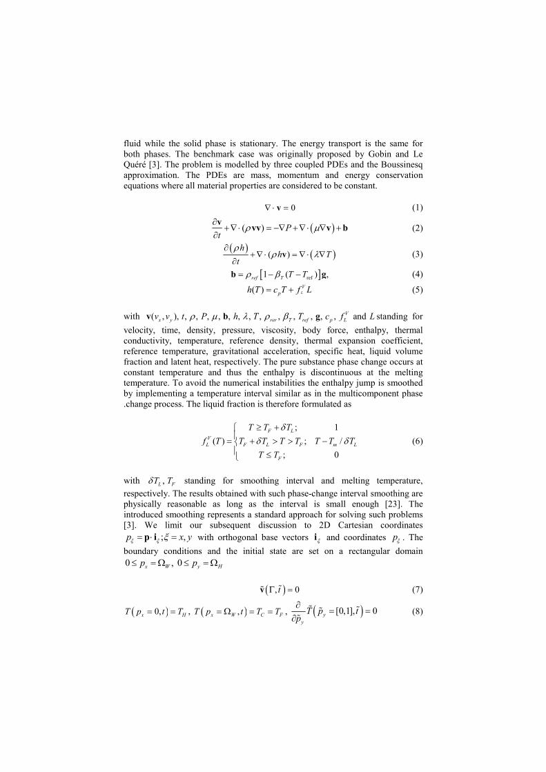
where , , , , , and ( , )H C W H x yT T p pΓ Ω Ω Ω p stand for hot side temperature, cold

side temperature, domain boundary, domain interior, domain width, domain height and position vector. The problem is characterized by four dimensionless numbers; thermal Rayleigh number, Prandtl number, Stefan number and domain aspect ratio defined as

( ) 3 2

Ra = T H C H p

T

T T cβ ρ

λµ

− Ωg, Pr pcµ

λ= ,

( )Ste= H CT T cp

L

−, RA W

H

D

D= . (11)

The problem is schematically presented in Figure 1.

Figure 1: Problem schematics.

3 Solution procedure

A two level Euler explicit time stepping scheme is used for time discretization. The domain and boundary are discretized into N N NΩ Γ= + nodes of which NΩ

nodes are distributed in the domain and NΓ at the boundary. The spatial

discretization is performed by using the local meshfree method where

overlapping local subdomains are used. An arbitrary scalar function θ is represented on each of the local subdomains as

1

( ) ( )BasisN

n n

n

θ α=

= Ψ∑p p (12)

where , andBasis n nN α Ψ stand for number of basis functions, interpolation

coefficients and basis functions, respectively. The basis could be selected arbitrary however in this work only Hardy’s Multiquadrics (MQs)

( ) ( ) ( ) 2/ 1n n

n CσΨ = − ⋅ − +p p p p p with Cσ standing for basis function free

shape parameter are used. For non refined node distributions even smallest five nodded subdomain collocation works fine but with introduction of more complex refined nodes distributions small subdomain computations do not behave convergent anymore. To circumvent the problem, larger subdomains are selected with more stable weighted least squares approximation to determine coefficients

nα . The subdomains are weighted by truncated Gauss weight function

2

0

2

0

exp( )( )

0

T

w

T

Wσ

σ

σ

− − ≤

= − >

pp p

p

p p

(13)

where 0, andT W

σ σ p stand for weight function truncation parameter, weight

function shape parameter and central subdomain node position vector, respectively. The subdomain size is thus determined by the weight function truncation radius, where all nodes within this radius are used as subdomain nodes. With the constructed approximation function an arbitrary spatial differential operator ( L ) can be computed

( )1

( )BasisN

n n

n

L Lθ α=

= Ψ∑p p . (14)

In the boundary nodes collocation instead of WLS is used in order to satisfy the boundary condition exactly [24]. In this paper five nodded subdomains are used in Neumann boundary nodes. In such nodes boundary node collocation equation is replaced by the boundary condition equation

1

( ) 0BasisN

n n

n

α=

∂Ψ =

∂∑ pn

. (15)

The spatial discretization problem is formulated in a vector form

1−=α Ψ Θ . (16)

with matrix dimension ( ) [ ]dim ,Sub BasisN N=Ψ where SubN stands for number of

subdomain nodes. To maintain the general formulation both, the WLS and the collocation are considered through equation (16) where pseudo inverse of the non square WLS matrix Ψ is computed by singular value decomposition and square collocation matrix is inverted by LU decomposition. With defined time and spatial discretization schemes the general transport equation under the model assumptions can be written as

( )21 00 0 0 0D S

t

θ θθ ρ

−= ∇ −∇Θ ⋅ +

∆v (17)

Where [ ]( )0,1 0 1,t tΘ = Θ stands for the field value in the interior node with index

Ω at current and next time step, D for general diffusion coefficient and 0SΩ for

source term. To couple the mass and momentum conservation a special treatment is required. The intermediate velocity is computed by

( )( )0 0 0 0 0 0ˆ ( )t

P µ ρρ∆

= + −∇ +∇ ⋅ ∇ + −∇ ⋅v v v b v v . (18)

The equation (18) did not take in account the mass continuity and therefore pressure and velocity corrections are added

1ˆ ˆm m+ = +v v v 1ˆ ˆm mP P P+ = +

(19)

where , andm v P

stand for pressure velocity iteration index, velocity correction

and pressure correction, respectively. Combining the momentum and mass continuity equations the pressure correction Poisson equation emerges

2ˆ m tP

ρ∆

∇ = ∇v

(20)

Instead of solving the global Poisson equation problem the pressure correction is directly related to the intermediate velocity divergence

2 ˆ mPt

ρ= ∇⋅

∆v

ℓ (21)

The proposed assumption enables direct solving of the pressure velocity coupling iteration and thus is very fast due to only one step needed in each node

to evaluate the new iteration pressure and the velocity correction. With computed pressure correction the pressure and the velocity can be corrected as

1ˆ ˆm m tPζ

ρ+ ∆= − ∇v v

1ˆ ˆm mP P Pζ+ = +

(22)

Where ζ stands for relaxation parameter. The iteration is performed until the

criteria ˆ· Vε∇ <v is met in all computational nodes.

Each simulation starts with the uniformly distributed initial nodes. At every

predefined number of time steps tN

Rσ all nodes are checked if

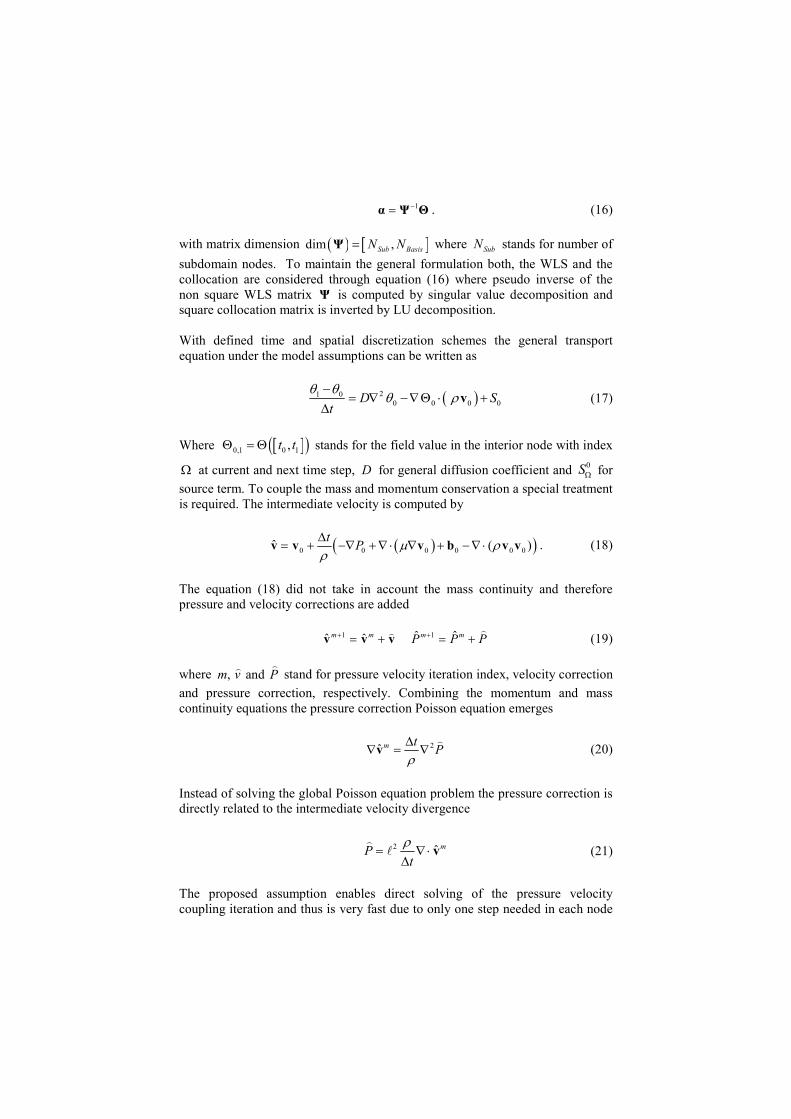
refinement/derefinement is needed. If the refinement criterion is met, additional nodes are added or removed from the vicinity of the node. At each refinement maximum four nodes are symmetrically added around the refined node. Maximum allowed difference in the refinements between neighbouring nodes is set to one in order to keep the numerical approach as stable as possible. Important part of CPU complexity of the meshfree methods represents the selection of proper subdomain. The problem becomes even more important when working with dynamic node distribution. Truly meshfree methods should not use any topological information about the nodes connectivity, however in order to utilize fast subdomain selection the information about the local node neighbourhood (four symmetric neighbours) is stored within the node. The example of once and four times refined node is presented in Figure 2 where the arrows point to each node neighbourhood.

Figure 2: An example of one refined node(left) and four time refined node

(right).

4 Results

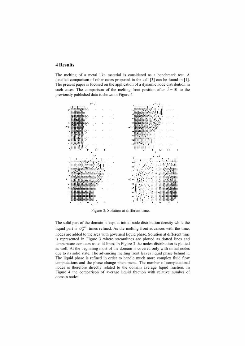
The melting of a metal like material is considered as a benchmark test. A detailed comparison of other cases proposed in the call [3] can be found in [1]. The present paper is focused on the application of a dynamic node distribution in such cases. The comparison of the melting front position after 10t =ɶ to the previously published data is shown in Figure 4.

Figure 3: Solution at different time.

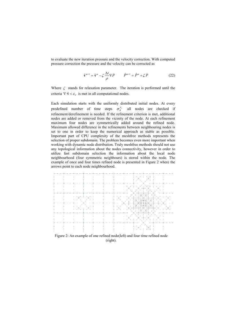
The solid part of the domain is kept at initial node distribution density while the

liquid part is maxR

σ times refined. As the melting front advances with the time,

nodes are added to the area with governed liquid phase. Solution at different time is represented in Figure 3 where streamlines are plotted as dotted lines and temperature contours as solid lines. In Figure 3 the nodes distribution is plotted as well. At the beginning most of the domain is covered only with initial nodes due to its solid state. The advancing melting front leaves liquid phase behind it. The liquid phase is refined in order to handle much more complex fluid flow computations and the phase change phenomena. The number of computational nodes is therefore directly related to the domain average liquid fraction. In Figure 4 the comparison of average liquid fraction with relative number of domain nodes

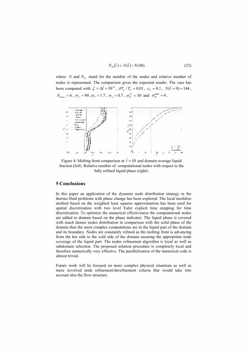
( ) ( ) / (40)DN t N t N=ɶ ɶ (23)

where and DN N stand for the number of the nodes and relative number of

nodes is represented. The comparison gives the expected results. The case has

been computed with 610tζ −= ∆ =ɶ , / 0.01L FT Tδ = , 0.1Vε = , ( 0) 144N t = =ɶ ,

6basisN = , 90Cσ = , 1.7Tσ = , 0.7wσ = , 50tN

Rσ = and max 6R

σ = .

Figure 4: Melting front comparison at 10t =ɶ and domain average liquid

fraction (left). Relative number of computational nodes with respect to the fully refined liquid phase (right).

5 Conclusions

In this paper an application of the dynamic node distribution strategy in the thermo-fluid problems with phase change has been explored. The local meshfree method based on the weighted least squares approximation has been used for spatial discretization with two level Euler explicit time stepping for time discretization. To optimize the numerical effectiveness the computational nodes are added to domain based on the phase indicator. The liquid phase is covered with much denser nodes distribution in comparison with the solid phase of the domain thus the most complex computations are in the liquid part of the domain and its boundary. Nodes are constantly refined as the melting front is advancing from the hot side to the cold side of the domain assuring the appropriate node coverage of the liquid part. The nodes refinement algorithm is local as well as subdomain selection. The proposed solution procedure is completely local and therefore numerically very effective. The parallelization of the numerical code is almost trivial. Future work will be focused on more complex physical situations as well as more involved node refinement/derefinement criteria that would take into account also the flow structure.

Acknowledgment

The authors would like to express their gratitude to Slovenian Research Agency for support in the framework of the projects Young Researcher Program 1000-06-310232 (G.K.), and project J2-0099 Multiscale Modelling and Simulation of Liquid-Solid Systems (B.Š.).

References

[1] Kosec, G. & Šarler, B., Solution of phase change problems by collocation with local pressure correction. CMES: Computer Modeling in

Engineering and Sciences, 47, pp. 191-216, 2009. [2] Kosec, G. & Šarler, B., Solution of thermo-fluid problems by collocation

with local pressure correction. International Journal of Numerical Methods for Heat and Fluid Flow, 18, pp. 868-882, 2008.

[3] Gobin, D. & Le Quéré, P., Melting from an isothermal verical wall, synthesis of a numerical comparison excercise. Comp. Assist. Mech. Eng.

Sc., 198, pp. 289-306, 2000. [4] Ferziger, J. H. & Perić, M., Computational Methods for Fluid Dynamics,

Springer: Berlin, 2002. [5] Ozisik, M. N., Finite Difference Methods in Heat Transfer CRC Press:

2000. [6] Shashkov, M., Conservative Finite-Difference Methods on General Grids,

CRC: Boca Raton, 1996. [7] Wrobel, L. C., The Boundary Element Method: Applications in Thermo-

Fluids and Acoustics, John Wiley & Sons: West Sussex, 2002. [8] Rappaz, M., Bellet, M. & Deville, M., Numerical Modeling in Materials

Science and Engineering, Springer-Verlag: Berlin, 2003. [9] Dantzig, J.A., Liquid-solid phase changes with melt convection.

International Journal of Numerical Methods in Engineering, 28, pp. 1769-1785, 1989.

[10] Viswanath, R. & Jaluria, R., A comparison of different solution methodologies for melting and solidification problems in enclosures. Numerical Heat Transfer, Part B, 24, pp. 77-105, 1993.

[11] Šarler, B. & Kuhn, G., Primitive variable dual reciprocity boundary element method solution of incompressible Navier-Stokes equations. Engineering Analysis with Boundary Elements, 23, pp. 443-455, 1999.

[12] Šarler, B. & Kuhn, G., Dual reciprocity boundary element method for convective-diffusive solid-liquid phase change problems, Part 2: Numerical Examples. Engineering Analysis with Boundary Elements, 21, pp. 65-79, 1998.

[13] Šarler, B. & Kuhn, G., Dual reciprocity boundary element method for convective-diffusive solid-liquid phase change problems, Part 1: Formulation. Engineering Analysis with Boundary Elements, 21, pp. 53-63, 1998.

[14] Šarler, B., Towards a mesh-free computation of transport phenomena. Engineering Analysis with Boundary Elements, 26, pp. 731-738, 2002.

[15] Kovačević, I. & Šarler, B., Solution of a phase-field model for dissolution of primary particles in binary aluminum alloys by an r-adaptive mesh-free method. Materials Science and Engineering A, 413–414, pp. 423–428, 2005.

[16] Perko, J. & Šarler, B., Weigh function shape parameter optimization in meshless methods for non-uniform grids. CMES: Computer Modeling in

Engineering and Sciences, 19, pp. 55-68, 2007. [17] Li, S., Petzold, L. & Ren, Y., Stability of moving mesh systems of partial

differential equations. Journal of Scientific Computing, 20, pp. 719-738, 1998.

[18] Bourantas, G.C., Skouras, E.D. & Nikiforidis, G.C., Adaptive support domain implementation on the moving least squares approximation for mfree methods applied on elliptic and parabolic pde problems using strong-form description. CMES: Computer Modeling in Engineering and

Sciences, 43, pp. 1-25, 2009. [19] Berger, M. J., Adaptive mesh refinement for hyperbolic partial differential

equations. Journal of Computational Physics, 53, pp. 484-512, 1983. [20] Berger, M. J. & Colella, P., Local adaptive mesh refinement for shock

hydrodynamics. Journal of Computational Physics, 82, pp. 64-84, 1989. [21] Mencinger, J., Numerical simulation of melting in two-dimensional cavity

using adaptive grid. Journal of Computational Physics, 198, pp. 243-264, 2003.

[22] De Vahl Davis, G., Natural convection of air in a square cavity: a bench mark numerical solution. International Journal of Numerical Methods in

Fluids, 3, pp. 249-264, 1983. [23] Dalhuijsen, A.J. & Segal, A., A comparison of finite element techniques

for solidification problems. Internation Journal of Numerical Methods in

Engineering, 23, pp. 1829-1986, 1986. [24] Kosec, G. & Šarler, B., Solution of heat transfer and fluid flow problems

by the simplified explicit local radial basis functon collocation method. 14th international Conference on FE in Flow Problems, pp. 2007.