INT06: Adaptive Percolation

Daniel Burkhardt CerigoSupervisors: Dr. Eduardo Lopez, Dr. Omar Guerrero

Word count: 7664

Abstract

The spread of infection is considered through percolation methods, including the case of a

new adaptive model. We set out the basic formalism for network analysis and contagion. The

SIS (Susceptible-Infected-Susceptible) model is analysed as a paradigm example of percolation

and more specifically contagion within a network. We present a generalised SIS model that

incorporates network adaptation to infection, reliant on the Popularity model of networks. The

adaptive SIS model is investigated computationally and the existence of a phase boundary is

established. A review of research on financial contagion is given and the lack of an adapted

element is noted. Implications and applications of the adaptive SIS model are given for areas

of financial contagion and epidemiology amongst others.

Contents

I Introduction 1

II Representing Networks 2II.1 The Configuration Model . . . . 3

III The SIS Model 3III.1 Model Specification . . . . . . . . 3III.2 Steady-State Infection Rates . . 4III.3 Discussion . . . . . . . . . . . . . 6

IVAdaptation 7IV.1 Review of Financial Contagion . 7

V The Popularity Model 8V.1 Model Specification . . . . . . . . 8V.2 Degree Distribution Analysis . . 9

VIAdaptive SIS Model 10VI.1 Model Specification . . . . . . . . 10VI.2 Results . . . . . . . . . . . . . . . 10VI.3 Discusion . . . . . . . . . . . . . 12

VII Conclusion 12

Appendices ii

A Example Degree Distributions ii

B Stochastic Ordering iii

C Further SIS Results iv

D Extended Financial Contagion Lit-erature Review v

E Degree Distributions from thePopularity Model vii

F Further Adaptive SIS Results viii

G Simulations x

I. Introduction

Network science is a blooming area of re-search with applications in a hugely broad rangeof fields leading to an active interdisciplinarymovement. The study of nature in networkframeworks dates back to the mathematicianEuler and his Seven Bridges, thus spawning themathematical study of networks called GraphTheory1. Later Paul Erdos and Alfred Renyi

1I use ‘graph’ when the discussion is within a more mathematical context but it can be taken as synonymous with‘network’.

1

published a series of seminal papers on ran-dom graphs in which they analytically deter-mined conditions for di↵ering levels of connec-tivity in their graphs [1–3]. The basic premiseof network science can be stated as: many partsof nature can be readily represented by net-works, these networks have clear pattens andstructures enabling various network classifica-tions, these patterns and structures have con-sequences for the systems they represent.

Examples of successful and varied applica-tions of network analysis include the friend-ship networks in schools dependence on ethnic-ity [4,5], representing interacting proteins in bi-ology [6], statistical mechanics of the networkformed by the internet [7], and even a proposedinfluence on an individual’s capability for in-novation due to properties of their network ofacquaintances [8].

Percolation is a specific subset of networkscience concerned generally with flow throughnetworks; this incorporates determining whenflow is possible, their rates, the ability for a net-work to sustain a spanning path when nodes orlinks are removed etc. In physics percolation isused in the study of phase transitions in sys-tems [9–12]. Its use in modelling and analysingthe spread of infectious disease in a populationis well developed [13–16], as well as more gen-eral ‘infections’ such as the spread of computerviruses, information or opinions through vari-ous networks structures like word-of-mouth in-teractions or email correspondences [17–19].

A limitation of these models is that theylack proper responsive dynamics; the networkstructure is una↵ected by the state of the sys-tem. This is reasonable in cases where the infec-tion is not apparent over timescales of transmis-sion such as for asymptomatic diseases, or whenthe infection simply doesn’t cause a change inthe behaviour of the host. But many systemsof contagion have an inherent adaptation; thosewith the common cold stay at home so are lesslikely to meet others and transmit the virus,or the spread of an opinion may be boostedby campaigners proactively persuading others.One area which has had a lot of recent successin applying percolation is modelling financialcrashes as the spread of collapse within a net-work of interdependent banking bodies [20–23].

It will be shown though that the models usedthus far do not incorporate an adaptive elementto capture the decision making and judgementof the participants involved in forming such eco-nomic ties.

In this paper we: 1. show the basic for-malism for network analysis and contagion,2. present a paradigm model of contagion; theSIS model, 3. we define adaptation within thenetwork context, 4. review the most visible pa-pers on financial contagion, 5. introduce a newmodel of network formation which lends itselfto adaptation, 6. present and computationallyanalyse an adaptive SIS model.

II. Representing Networks

A network consists of a set of nodes (vertices,agents)N = {1, . . . , n} and a set of links (edges,connections) G = {{i, j} : i, j 2 N}. The set oflinks can also be represent by an n ⇥ n matrixcalled an adjacency matrix ;

gij

=

(1, if {i, j} 2 G,

0, otherwise.

We will only consider simple, undirected andunweighted networks meaning no self-links,links are always two-way, and all links areequivalent respectively. This requires g

ii

= 0for all i, g to be symmetric, and g to containonly 1’s or 0’s.

The degree di

of a node i is the number oflinks containing it or equivalently the numberof nodes i is linked to. Formally

di

= |{j|{i, j} 2 G}| =X

j

gij

.

The degree distribution P of a network is acentral object in the characterisation and anal-ysis of networks. It describes the relative fre-quency of nodes of each degree. Given such adistribution, then P (d) is the fraction of nodesthat have degree d. Note that the degree dis-tribution can be a probability distribution fromwhich we can generate a set of degrees to forma network, or it can be a frequency distributionused to describe data from an actual network.

Common degree distributions, which wewill be considering, are the delta distribution

2

P (d) = �dk

which forms a regular network inwhich all nodes have the same degree k. The

Poisson distribution2, P (d) = �

d

d! e�� where � is

the mean degree, which form Erdos-Renyi net-works3 (ER for short). Lastly the scale-free dis-tribution (SF for short), P (d) = cd�� where cis a normalisation factor, which produces scale-free networks. SF networks di↵er from ER net-works in that they tend to have many more veryhigh degree nodes and very low degree nodes;the network has a large spread of degrees. Eachof these network structures are observed in realworld systems [24–26]. See Appendix A forplots of these distributions.

The mean degree and second moment of anetwork with P are given by hdi =

Pd

P (d)dand hd2i =

Pd

P (d)d2 respectively. Di↵usionthrough a network increases with increasinghdi [27] since there are more links in the net-work through which it is possible to flow. So tocompare aspects of percolation just between thestructures of various networks, we do so whileholding their average degrees constant. An im-portant result is that (while holding the meanconstant) hd2i increases with increasing spreadin the degree distribution P (d) [27], called amean-preserving spread. The regular degreedistribution has no spread, the Poisson hassome and the scale-free even more so; this ismost visible in Appendix A Figures 12 and 14.This creates an ordering when holding the meanconstant; hd2i

�

< hd2iPo.

< hd2iSF

, the Pois-son distribution is a mean-preserving spread ofthe delta distribution and the scale-free distri-bution is a mean-preserving spread of both. SeeAppendix B for further explanation on the or-dering of distributions through stochastic dom-inance.

II.1. The Configuration Model

The configuration model is a procedure bywhich, given a degree distribution, we can forma random network with corresponding degree

frequencies.i) Take n samples from a given de-

gree distribution to form a degree sequence{d1, d2, . . . , dn}. ii) Construct the sequencewhere node i is listed d

i

times; the degree se-quence {41, 12, . . . , 6n} would result in

{1, 1, 1, 1, 2, . . . , n, n, n, n, n, n}.

iii) Repeat the following steps until the list isempty: 1. pick two elements at random4, 2.form the link between the two nodes repre-sented by the pair of elements, 3. delete theelements. This provides a method of forming arandom network with a given degree distribu-tion.

Problems inherent in the configurationmodel are the possibilities of more than one linkforming between two nodes, and links connect-ing a node to itself. The chance of these occur-ring become increasingly small for large n anda sparse network (d

max

⌧ n); we can form anapproximate network by removing any multipleor self-links that happen to occur.

III. The SIS Model

III.1. Model Specification

The SIS model is not a fixed network of nodesbut an application of network theory to modela collection of agents who have random interac-tions or meetings with one another overtime, inwhich an abstract infection can be transmitted.

Consider a collection of agents representedby nodes, all of which can be in one of twostates; susceptible or infected. Agents are neverremoved from the system but recover from in-fection to return to the susceptible state (henceSusceptible-Infected-Susceptible or SIS). Eachagent is described by their degree; the i ’th agenthas degree d

i

. The degree describes the num-ber of interactions with other random agentsthey will have within a given period, so we callthe SIS model a degree-based random meetingmodel. One should think of the SIS model as a

2This distribution is actually an approximation of the distribution formed in the random graphs studied byErdos and Renyi [1–3]. Take n nodes and form links between them with probability p; this gives a binomial degree

distribution P (d) =�n�1d

�p

d(1� p)n�1�d. For large n and small p this approximates to the Poisson distribution.3There are varies elements of randomness in the models considered and to avoid ambiguity we will not call ER

networks ‘random’ networks as is the case in much literature.4It is assumed without real problem for large n that this sequence is even in length.

3

network defined by a given degree distributionwhich after every period of time is completelyremade randomly. Nodes which are linked inthe network for that period denote agents thatmeet during that period.

We define the infection density ⇢(d) to bethe fraction of agents with degree d that areinfected. Let P

m

(d) be the probability of meet-ing an agent of degree d, and ✓ be the prob-ability that a given interaction is with an in-fected node; then ✓ =

Pd

Pm

(d)⇢(d). For asparse network of large n formed using the con-figuration model, the degree of neighbouringnodes are approximately uncorrelated. Thenthe probability of meeting an agent of each de-gree P

m

(d) is the same as the number of linksinvolving nodes of degree d – P (d)dn – nor-malised by the total number of links in the sys-tem

Pd

P (d)dn. Thus Pm

(d) = P (d)dPd P (d)d =

P (d)dhdi , and so meetings are more likely to be

with higher degree agents [15]. This leads to

✓ =X

d

⇢(d)P (d)d

hdi . (1)

We define the average infection rate5 ⇢ asthe total fraction of agents in the model thatare infected at a given time: ⇢ =

Pd

P (d)⇢(d).This di↵ers from ✓ because an individual ismore likely to meet another agent if that agenthas many meetings.

The final probability of an agent being in-fected within a given period will be some func-tion of ✓, the agent’s degree and other parame-ters describing the specifics of the infection me-chanics. For instance the infection could trans-mit with certainty in meetings between infectedand susceptible nodes, or there could be prob-ability of infected per such a meet, or even athreshold on the number of such meetings re-quired for transmission. We choose the simpleform of a transmission rate parameter ⌫ 2 [0, 1],which is the probability for transmission of in-fection in a given meeting between an infectedand a susceptible agent. So the final probability

for infection in a period is6

⌫✓d. (2)

We choose recovery to be a simple Marko-vian property that is the same for all agents: achance of recovery per period equal to � 2 [0, 1].

Simulated evolution of this system can beseen in Appendix C.

III.2. Steady-State Infection Rates

Assume a mean-field approximation such thateach agent has a fraction of infected neighbour-ing nodes that matches exactly the density ofinfected nodes ⇢(d). The number that recover isthe fraction that are infected multiplied by therecovery rate, and the number that become in-fected is the number of susceptible agents mul-tiplied by the probability of infection in a givenperiod. So @⇢(d)

@t

= (1 � ⇢(d))⌫✓d � ⇢(d)�. We

then solve for steady-states @⇢(d)@t

= 0, so solv-ing for when the number recovering in a periodis equal to the number that become infected.This leads to the steady-state equation

(1� ⇢(d))⌫✓d = ⇢(d)�. (3)

Let � = ⌫

�

. Solving for infection density gives

⇢(d) =�✓d

(�✓d+ 1). (4)

Substituting this into (1) gives the definingequation for the infection rate ✓ for the modelin a steady-state

✓ =X

d

P (d)�✓d2

hdi(�✓d+ 1). (5)

Remarks; i) ✓ = 0 is always a solution cor-responding to the steady-state of no infection.ii) ✓ < 1 for finite �. iii) The righthand side of(5) is an increasing and convex function of d.The steady-states can be solved exactly for aregular network of degree k; P (d) = �

dk

giving

✓ =X

d

�dk

�✓d2

hdi(�✓d+ 1)=

�✓hdi�✓hdi+ 1

= ⇢(k), (6)

5The notation for infection densities ⇢(d) compared with the average infection rate ⇢ is only distinguished by thepresence or lack of the argument (d). This becomes more intuitive once one realises that there are multiple infectiondensities at any one time, one for each degree, but just one unique average infection at such a time.

6Choosing ⌫ such that max(d)⌫ ⌧ 1 keeps the probability of infection per period well defined.

4

where the last equality follows from (4). Again✓ = 0 is a solution. Cancelling a factor of ✓ from(6) then rearranging gives a second solution

✓ = 1� 1

�hdi , (7)

giving a threshold for a non-zero steady infec-tion in a regular network

hdi > 1

�. (8)

This result fits with the intuition that higher in-fection to recovery ratio � requires a less denselyconnected network to sustain an infection. Thevalue of the threshold determines the point atwhich the system undergoes a phase transition,from being capable of sustaining an infectionand not.

The analytical formula for the average infec-tion of a regular network is also easily derived:

⇢ =X

d

P (d)⇢(d) = ⇢(k) = ✓. (9)

So it follows that for a non-zero steady stateinfection in a regular network the average in-fection is equal to and has the exact form asthe infection rate from (7), which is to be ex-pected as the network is uniform; there is anequal probability of meeting any node in a giveninteraction.

Lopez-Pintado [14] derive a general thresh-old for non-zero steady-state infections as fol-lows. Define the infection rate evolution func-tion

H(✓) =X

d

P (d)�✓d2

hdi(�✓d+ 1). (10)

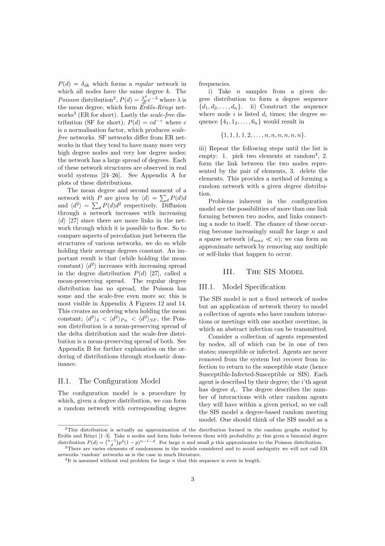
Remarks; i) H(✓) > ✓ corresponds to increas-ing infection rate, ii) H(✓) < ✓ to decreasing.iii) H(✓) = ✓ corresponds to the system beingin a steady-state. iv) H(0) = 0 is always astead-state as previously noted. v) H(✓) is anincreasing and strictly concave function of ✓.

Due to the strictly concave property of theevolution function (and both H(✓) and ✓ be-ing bounded by [0, 1)), any H(✓) that beginsabove the line H(✓) = ✓ must necessarily inter-sect that very line at a higher value for ✓, lead-ing to the existence of a non-zero steady-state.Conversely any H(✓) that begins below the line

H(✓) = ✓ cannot possibly intersect it showinga non-zero steady-state is impossible. Thesetwo cases are exactly determined by whetherH 0(0) > 1 or H 0(0) < 1 respectively. This rea-soning is show diagrammatically in Figure 1.

Figure 1: Diagrammatical explication; the gradientof H(✓) at 0 determines the existence of a non-zero steady-state infection rate. Reproduced fromM.O.Jackson [28].

Since

H 0(✓) =X

d

P (d)d2

hdi1

(�✓d+ 1)2, (11)

and

H 0(0) = �hd2ihdi , (12)

thus the general threshold for a non-zerosteady-state is

� >hdihd2i . (13)

For the regular network hdi2 = hd2i, so the re-sult in (8) is recovered. For the Poisson dis-tribution we have hd2i = hdi2 + hdi giving athreshold

� =1

1 + hdi . (14)

For a system of infinite size, the scale-free distri-bution has a divergent hd2i and so will in theorybe able to sustain a non-zero infection for anypositive �.

State stability is also readily determined byH 0(0). For a small fluctuation in infection rate" (akin to introducing infection in the system),if H 0(0) > 1 then H(") > " and so the infectionrate diverges from zero untill it reaches it’s non-zero steady-state which is stable to fluctuations.

5

If H 0(0) < 1 then H(") < " so fluctuations dieand the steady-state with zero infection is sta-ble.

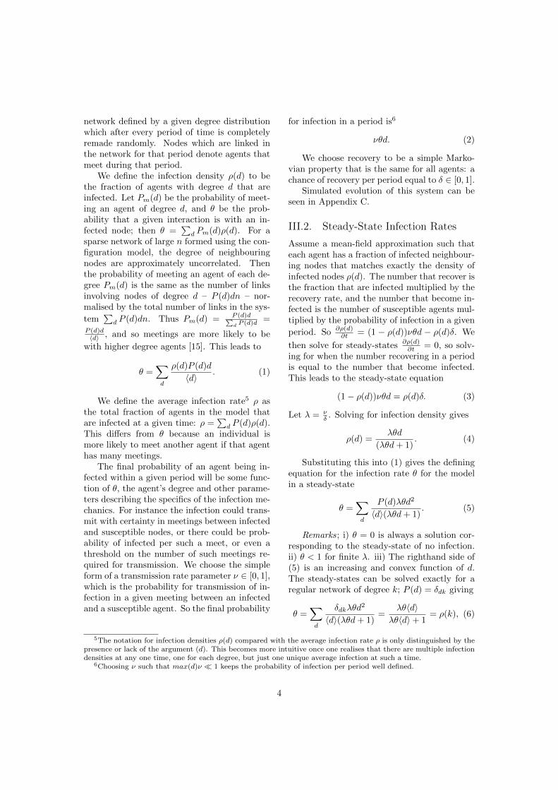
Figure 2: Thresholds for non-zero steady-state in-fections while varying average degree for various de-gree distributions, with n = 1000.

Figure 2 shows the theoretical predictions ofthe thresholds for varying average degree for thedegree distributions discussed, and the agreeingresults from simulation7. The thresholds signif-icantly above 0 for the scale-free distribution,which goes against (13), are a result of simulat-ing a finite system.

For a given average degree, the orderingof the thresholds of the distributions corre-sponds to the opposite of the mean-preservingspread ordering discussed in Section II, becausethe threshold is inversely proportional to hd2i;�SF

< �Po.

< ��

. For average degree greaterthan 2, distinguishing di↵erences in dynamicsbetween the distributions requires a high reso-lution of �. Because of this we will now lookprimarily at networks with hdi = 2, which ex-hibit the most variable dynamics over a largerange of �.

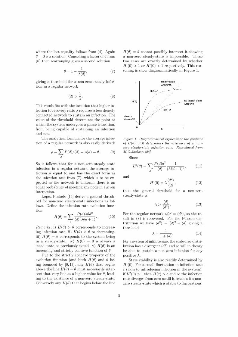
Figure 3 plots the theoretical change insteady-state average infection with � for theregular network from (6), with the simulatedsteady-state infection rates for all three ofthe distributions discussed. Remarks: i) Thethreshold values of � are as predicted by (13);for low �, ⇢

�

< ⇢Po.

< ⇢SF

, the greater spreadin degree leads to greater ability to sustain in-fection. ii) For high � this ordering is reversed;⇢SF

< ⇢Po.

< ⇢�

, so the less spread distribu-tions sustain a higher average infection.

Figure 3: Average infection rate for varying �, andvarious degree distributions, with n = 1000 andhdi = 2.

This phenomena is predicted theoreticallyby Jackson [29], and has an intuitive expla-nation. In a network with large spread in itsdegrees there will exist many significantly iso-lated nodes, as well as a subnetwork of highlyconnected nodes with a significantly higher av-erage degree than for the network as a whole.As Figure 2 shows that the thresholds decreaserapidly with increasing average degree, so thissubnetwork can sustain an infection for low �and the infection will be mostly contained tothe subnetwork. At high � a densely connectedsubnetwork is no longer required and infectioncan propagate through the whole network, yetthe very isolated nodes are still highly unlikelyto be infected often reducing the steady-state ⇢;this is not the case for a regular network whichdoes not contain any significantly isolated nodesand so results in a higher ⇢.

III.3. Discussion

Key conclusions: i) There exist precise thresh-olds for non-zero steady-state infections whichare dependent on the degree distribution of anetwork. ii) Predictions for the ordering ofthresholds and steady-state average infectionrate is possible in the low and high � rangebased on ordering of the degree distributionsby spread.

The model and the derived results can bereadily used for prediction and guiding policymaking in the areas of health care, immunisa-tion, cyber security and opinion spreading, but

7The complete code for all simulations used can be found in Appendix G.

6

they also have further implications than theirgeneral predictive ability. For instance, thoughsystems which exhibit scale-free network struc-ture can maintain an infection even with smalltransmition rates/high recovery rates, they aremuch more susceptible to targeted vaccinationthan networks with less degree variance. In thescale-free case it would only be required to im-munise the relatively small fraction of highlyconnected nodes for the infection to die out,compared with a much larger fraction of theequally important nodes in a regular network.

There are a number of limitations of thestandard SIS model. Firstly, the networksformed using the configuration model result inneighbours having approximately independentdegrees and so not exhibiting any of the de-tailed network structures seen in real networks,such as nodes clustering into groups and loopsof linked nodes. Secondly, the network forma-tion is independent of the state of the infectionwithin the system. This fails to properly cap-ture any e↵ects infection may have on a host’sconnectivity, as well as any decision makingprocess by agents involved in forming a bond.For instance agents may actively avoid meetinginfected agents. This last point in especiallyrelevant to economic interactions in which tiesare generally formed with a definite purpose,and is dependent upon the reliability of partiesinvolved.

IV. Adaptation

We aim to tackle the last limitation noted forthe SIS model in Section III.3; the SIS model’slack of a reactive element to infection. We chosethe SIS model initially because it is well suitedto incorporating adaptation due to the repeatednetwork breakdown and formation used to rep-resent the random meetings.

We define adaptation as any change in thenetwork structure in response to the state ofpart, or the whole of the system. So link re-moval, creation and rewiring, in direct responseto an infection within the network is an exam-

ple of adaptation. There is large scope for avariety of adaptations8. We choose to focus ona single adaptation in which infection is seenas a disadvantage, and thus agents attempt toavoid interactions with other infected agents,or equivalently infected agents have a reducedconnectivity. Once an agent has recovered theyalso recover their initial level of connectivity.We call the generalised form of the SIS modelthat contains an adaptive element an adaptiveSIS model.

There is empirical motivation for an adap-tation of this type. Illness can naturally limita host’s exposure to others, and in some situ-ations people can autonomously avoid meetinginfected others. Anti-virus software can iden-tify sites/emails which are likely to contain ma-licious software to help users avoid them. En-tities forming economic ties make judgementsof opposing parties and aim to avoid those thatare unstable or failing.

Among the contexts in which adaptation isrelevant, one of the most visible and rapidlyexpanding areas is financial contagion; study-ing the collapse of financial systems as conta-gion of failure through a network of connectfinancial bodies. The e↵ects of financial col-lapses are detrimental across entire populationsof the developed world making its investigationa high priority for policy makers and govern-ments. Financial systems are inherently math-ematical and evolve through (generally) logicaldecision-making, therefore adaption is a vitalcomponent of them. Despite this, the most vis-ible papers on the subject do not contain anadaptive element, as shown in the following re-view.

IV.1. Review of Financial Contagion

Financial crises over the past decades have mo-tivated attempts at understanding the causesand mechanisms responsible by modelling fi-nancial collapses as contagion through a net-work of connected financial bodies (‘bank’ forshort). In this section I aim to introduce the

8We can di↵erentiate between two types of adaptation; system-wide and local. A system-wide adaptation wouldbe a change applied uniformly to every node or link in the system. For instance, uniformly reducing the degree ofevery node in the network once a certain average infection rate is reached would be a system-wide adaptation. Alocal adaptation is determined and applied at the level of individual nodes or links; once a node becomes infected itreduces it’s degree by one, would be an example.

7

reader to the most visible papers and highlighttheir most common aspects. See Appendix Dfor a more in-depth review.

1. Financial Contagion - Allen, Gale (2000)[20]. The authors aim to establish whetherfinancial collapse can be explained by conta-gion across a network of interdependent banks.They apply economic theory to establish a prof-itably optimal system of interbank loans be-tween four banks. A bank is then shockedby an unexpectedly large set of deposit with-drawals causing the bank to default. The ini-tial bank default deterministically transmits aloss to each of the banks it it indebted to,causing those to default in some cases; thismechanism of contagion is called counterpartloss. The authors establish that it is econom-ically understandable that banks form systemsin which bank default can be transmitted toothers through counter party losses.

2. Network Models and Financial Stabil-ity - Nier et al. (2007) [21]. The authorsaim to investigate how the structure of finan-cial networks a↵ects its susceptibility to sys-tematic breakdown. They model the finan-cial system as a random network representingbanks and their interbank loaning. A bank isshocked/made to default at random and thisloss transmits through interbank loans (links)via counter party loss. The extent of collapsein the network is analysed for varying networkconnectivity, size of loan per connection, sizeof each banks bu↵er to losses, and system size.The results show non-monotonic changes in theextent of contagion with increasing connectiv-ity, amongst others.

3. Stability Analysis Of Financial Conta-gion due to Overlapping Portfolios - Caccioli etal. (2014) [23]. The authors aim to investigatethe stability of a system of banks investing ina set of assets. They model the system as arandom bipartite9 network of banks and assets.Banks default once they incur enough losses onassets. Defaulted banks sell all their assets andthe worth of an asset falls as quantities of it aresold, thus transmitting losses through overlap-ping assets leading to more defaults. Stabilityis investigated by computing the probability ofsystem collapse for varying parameters. The

authors show the existence of various systemphase transitions.

The preceding papers all investigate closelyrelated questions, and so contain common ele-ments.

Elements common to all models: i) Staticrandom network. ii) Infection is transmitteddeterministically through network links basedon the properties of nodes. iii) Nodes do notrecover. iv) There is no network reaction to in-fection. For a fully relevant model of financialcontagion which can be used in policy making,some form of an adaptive element is required.

There a number of significant di↵erences in-herent in the SIS model compared to financialcontagion models: i) Random meeting model,not a static random network. ii) Infectionis transmitted randomly, not deterministicallybased on the properties of nodes. iii) Nodesrecover from infection.

We do not propose that an adaptive SISmodel is an actual model of financial contagion.Our aim is to make initial ground by presentinga simple but extendable adaptive model of con-tagion generally, though it could be used as anexample for incorporating adaptation in modelsof financial contagion in the future.

V. The Popularity Model

The configuration model and its use of degreedistributions is relatively unsuited for an agent-based adaptation. Firstly altering a node’s de-gree, based on its infected/susceptible state,must be a discrete process. And altering thedegree distribution is a system-wide adaptation.We propose the following model, which allowsfor a continuous change in the connectivity ofa single node, as a candidate to incorporateagent-based adaptation.

V.1. Model Specification

This model is a generalisation of the Erdos-Renyi model. In the ER model, links are formedwith a probability p. In the popularity modeleach node is associated with a popularity; linkij is formed with a probability which is a func-tion of the popularities of the nodes i and j.

9A bipartite network consists of two sets of nodes, and links are only formed between nodes in di↵ering sets.

8

Define P (p) to be a probability distributionover p 2 [0, 1], called a popularity distribution;this replaces the degree distribution used in Sec-tion II as the defining object in the structureof a network. Random networks with n nodesand P (p) are formed as follows10: i) Take nsamples from P (p) to form a sequence of popu-larities {p1, p2, . . . , pn}. ii) Form links ij withprobability p

i

pj

;

Prob(ij) = pi

pj

. (15)

V.2. Degree Distribution Analysis

Even though the degree distribution is not adefining object of networks in the popularitymodel, it is still central in the analysis of theresultant networks, and enables comparison tonetworks formed using the configuration model.

Average Degree: Given n nodes and popu-larity distribution P (p), the average degree ofnode i is

di

= pi

X

j 6=i

pj

, (16)

which for large n is approximately

di

= pi

n

Z 1

0P (p)p dp = p

i

nhpi. (17)

Averaging this over all nodes is the averagedegree for the network, and using the same ap-proximation gives

hdi =P

i

di

n=

n2hpiR 10 P (p)p dp

n= nhpi2.

(18)Exact forms of higher order moments re-

quire a complete form of the degree distribu-tion.

Degree Distributions: Let P ={p1, p2, . . . , pn} be the probability sequence fora network. Let Q = {{p

i

, pj

}|pi

, pj

2 P} be theset of all subsets of P with cardinality two (allpairs of popularities). The exact form of the

degree distribution is

P (d) =X

|S✓Q|=d

Y

{pi,pj}2S

pi

pj

Y

{pk,pl}2Q\S

(1�pk

pl

).

(19)If p

i

= p for all i, the distribution reduces tothe binomial distribution with a probability ofsuccess per trail p2. Thus the popularity modelwith constant popularity rightly reduces to theErdos-Renyi model.

Though the exact form of the degree distri-bution may not be intractable, initial analysiscan be easily gain through computationally cre-ating networks using the popularity model andanalysing the resultant degree distributions di-rectly.

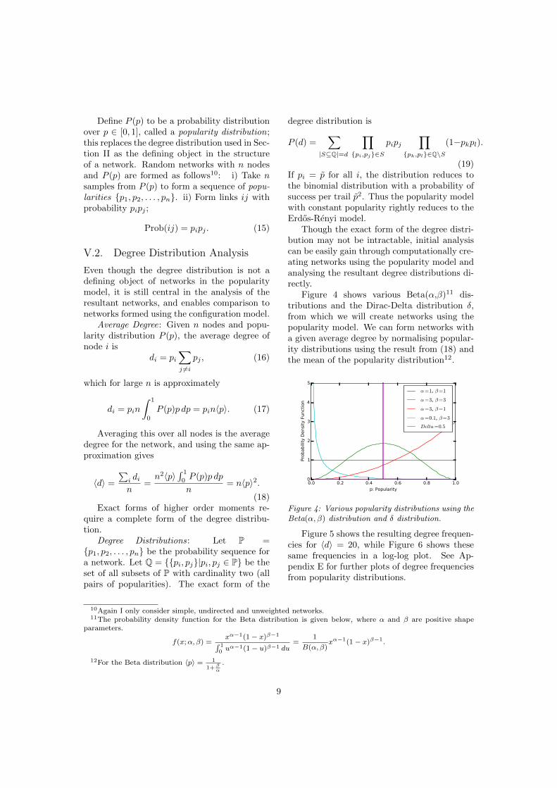
Figure 4 shows various Beta(↵,�)11 dis-tributions and the Dirac-Delta distribution �,from which we will create networks using thepopularity model. We can form networks witha given average degree by normalising popular-ity distributions using the result from (18) andthe mean of the popularity distribution12.

Figure 4: Various popularity distributions using theBeta(↵,�) distribution and � distribution.

Figure 5 shows the resulting degree frequen-cies for hdi = 20, while Figure 6 shows thesesame frequencies in a log-log plot. See Ap-pendix E for further plots of degree frequenciesfrom popularity distributions.

10Again I only consider simple, undirected and unweighted networks.11The probability density function for the Beta distribution is given below, where ↵ and � are positive shape

parameters.

f(x;↵,�) =x

↵�1(1� x)��1

R 10 u

↵�1(1� u)��1du

=1

B(↵,�)x

↵�1(1� x)��1.

12For the Beta distribution hpi = 1

1+ �↵

.

9

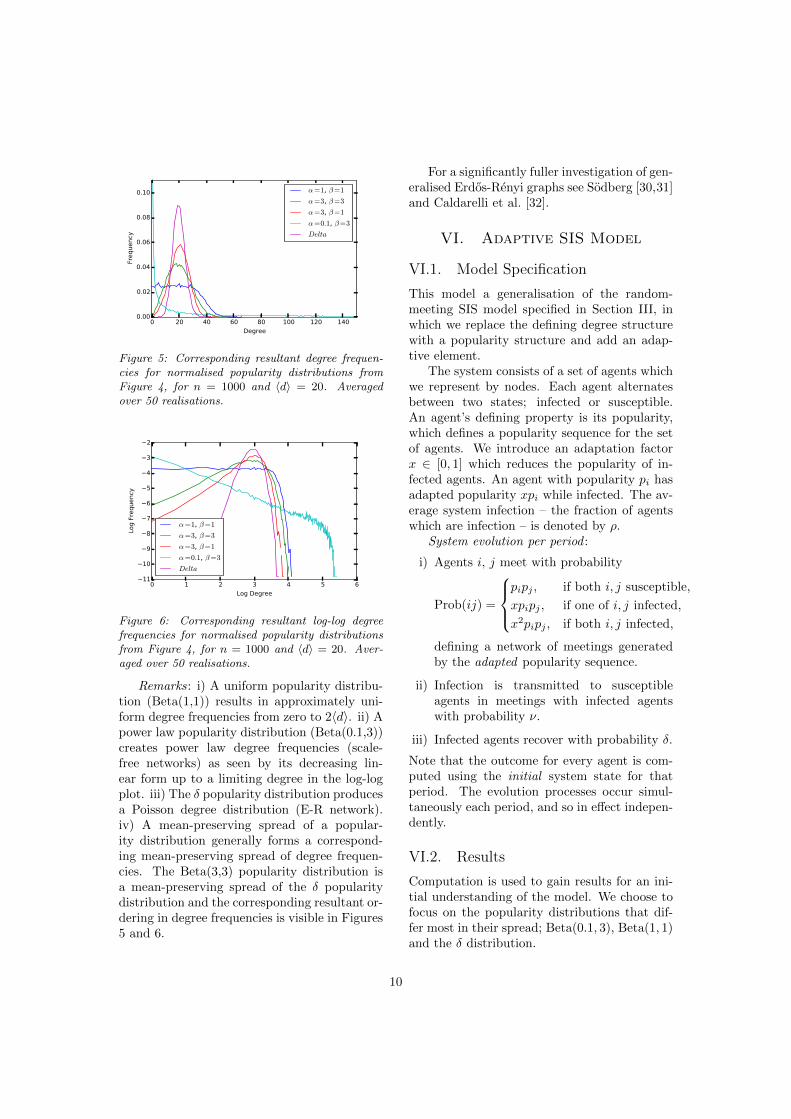
Figure 5: Corresponding resultant degree frequen-cies for normalised popularity distributions fromFigure 4, for n = 1000 and hdi = 20. Averagedover 50 realisations.

Figure 6: Corresponding resultant log-log degreefrequencies for normalised popularity distributionsfrom Figure 4, for n = 1000 and hdi = 20. Aver-aged over 50 realisations.

Remarks: i) A uniform popularity distribu-tion (Beta(1,1)) results in approximately uni-form degree frequencies from zero to 2hdi. ii) Apower law popularity distribution (Beta(0.1,3))creates power law degree frequencies (scale-free networks) as seen by its decreasing lin-ear form up to a limiting degree in the log-logplot. iii) The � popularity distribution producesa Poisson degree distribution (E-R network).iv) A mean-preserving spread of a popular-ity distribution generally forms a correspond-ing mean-preserving spread of degree frequen-cies. The Beta(3,3) popularity distribution isa mean-preserving spread of the � popularitydistribution and the corresponding resultant or-dering in degree frequencies is visible in Figures5 and 6.

For a significantly fuller investigation of gen-eralised Erdos-Renyi graphs see Sodberg [30,31]and Caldarelli et al. [32].

VI. Adaptive SIS Model

VI.1. Model Specification

This model a generalisation of the random-meeting SIS model specified in Section III, inwhich we replace the defining degree structurewith a popularity structure and add an adap-tive element.

The system consists of a set of agents whichwe represent by nodes. Each agent alternatesbetween two states; infected or susceptible.An agent’s defining property is its popularity,which defines a popularity sequence for the setof agents. We introduce an adaptation factorx 2 [0, 1] which reduces the popularity of in-fected agents. An agent with popularity p

i

hasadapted popularity xp

i

while infected. The av-erage system infection – the fraction of agentswhich are infection – is denoted by ⇢.

System evolution per period :

i) Agents i, j meet with probability

Prob(ij) =

8><

>:

pi

pj

, if both i, j susceptible,

xpi

pj

, if one of i, j infected,

x2pi

pj

, if both i, j infected,

defining a network of meetings generatedby the adapted popularity sequence.

ii) Infection is transmitted to susceptibleagents in meetings with infected agentswith probability ⌫.

iii) Infected agents recover with probability �.

Note that the outcome for every agent is com-puted using the initial system state for thatperiod. The evolution processes occur simul-taneously each period, and so in e↵ect indepen-dently.

VI.2. Results

Computation is used to gain results for an ini-tial understanding of the model. We choose tofocus on the popularity distributions that dif-fer most in their spread; Beta(0.1, 3), Beta(1, 1)and the � distribution.

10

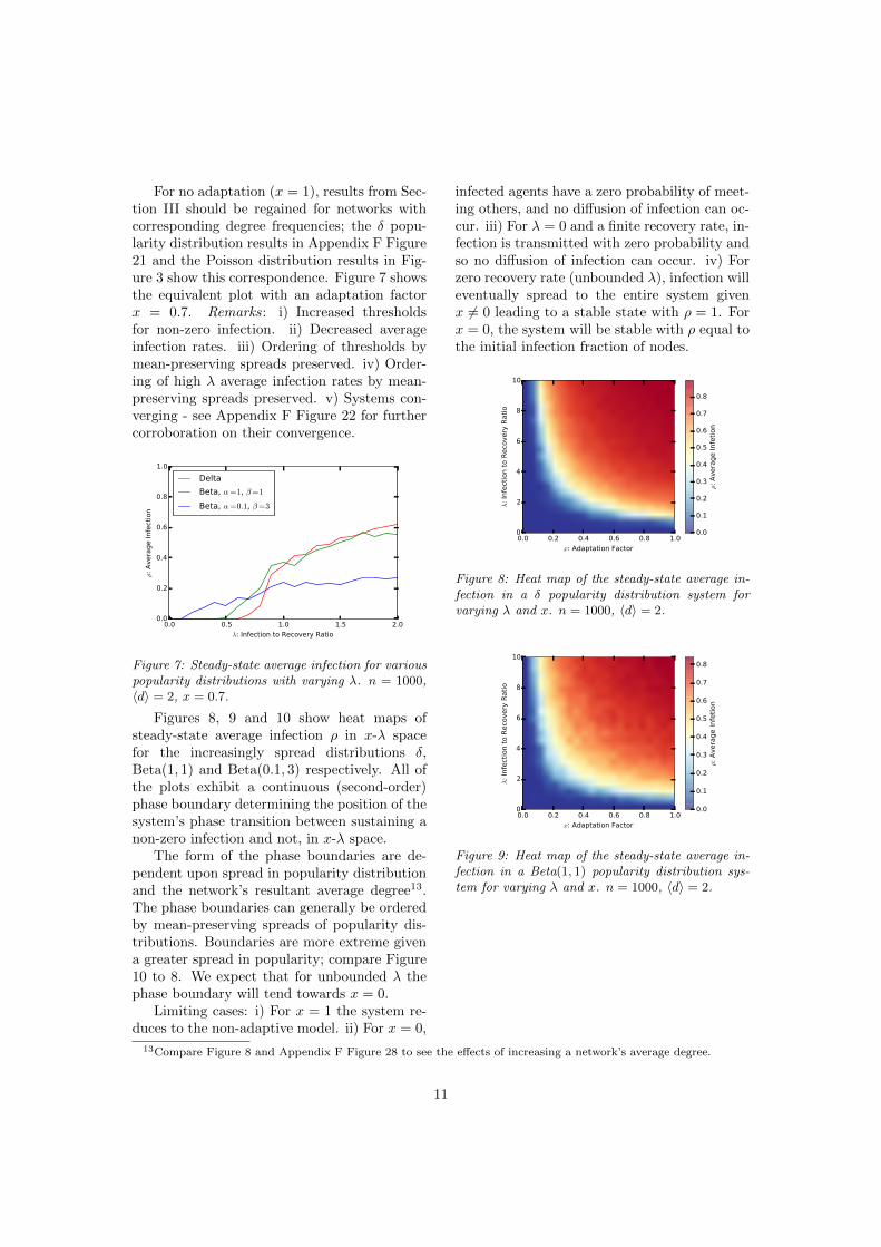
For no adaptation (x = 1), results from Sec-tion III should be regained for networks withcorresponding degree frequencies; the � popu-larity distribution results in Appendix F Figure21 and the Poisson distribution results in Fig-ure 3 show this correspondence. Figure 7 showsthe equivalent plot with an adaptation factorx = 0.7. Remarks: i) Increased thresholdsfor non-zero infection. ii) Decreased averageinfection rates. iii) Ordering of thresholds bymean-preserving spreads preserved. iv) Order-ing of high � average infection rates by mean-preserving spreads preserved. v) Systems con-verging - see Appendix F Figure 22 for furthercorroboration on their convergence.

Figure 7: Steady-state average infection for variouspopularity distributions with varying �. n = 1000,hdi = 2, x = 0.7.

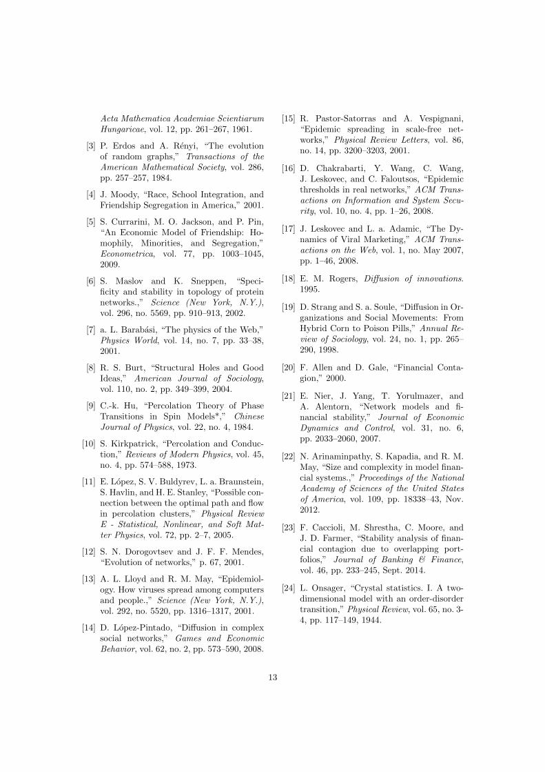
Figures 8, 9 and 10 show heat maps ofsteady-state average infection ⇢ in x-� spacefor the increasingly spread distributions �,Beta(1, 1) and Beta(0.1, 3) respectively. All ofthe plots exhibit a continuous (second-order)phase boundary determining the position of thesystem’s phase transition between sustaining anon-zero infection and not, in x-� space.

The form of the phase boundaries are de-pendent upon spread in popularity distributionand the network’s resultant average degree13.The phase boundaries can generally be orderedby mean-preserving spreads of popularity dis-tributions. Boundaries are more extreme givena greater spread in popularity; compare Figure10 to 8. We expect that for unbounded � thephase boundary will tend towards x = 0.

Limiting cases: i) For x = 1 the system re-duces to the non-adaptive model. ii) For x = 0,

infected agents have a zero probability of meet-ing others, and no di↵usion of infection can oc-cur. iii) For � = 0 and a finite recovery rate, in-fection is transmitted with zero probability andso no di↵usion of infection can occur. iv) Forzero recovery rate (unbounded �), infection willeventually spread to the entire system givenx 6= 0 leading to a stable state with ⇢ = 1. Forx = 0, the system will be stable with ⇢ equal tothe initial infection fraction of nodes.

Figure 8: Heat map of the steady-state average in-fection in a � popularity distribution system forvarying � and x. n = 1000, hdi = 2.

Figure 9: Heat map of the steady-state average in-fection in a Beta(1, 1) popularity distribution sys-tem for varying � and x. n = 1000, hdi = 2.

13Compare Figure 8 and Appendix F Figure 28 to see the e↵ects of increasing a network’s average degree.

11

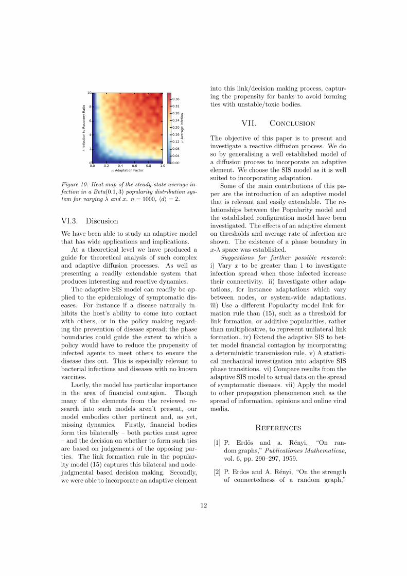
Figure 10: Heat map of the steady-state average in-fection in a Beta(0.1, 3) popularity distribution sys-tem for varying � and x. n = 1000, hdi = 2.

VI.3. Discusion

We have been able to study an adaptive modelthat has wide applications and implications.

At a theoretical level we have produced aguide for theoretical analysis of such complexand adaptive di↵usion processes. As well aspresenting a readily extendable system thatproduces interesting and reactive dynamics.

The adaptive SIS model can readily be ap-plied to the epidemiology of symptomatic dis-eases. For instance if a disease naturally in-hibits the host’s ability to come into contactwith others, or in the policy making regard-ing the prevention of disease spread; the phaseboundaries could guide the extent to which apolicy would have to reduce the propensity ofinfected agents to meet others to ensure thedisease dies out. This is especially relevant tobacterial infections and diseases with no knownvaccines.

Lastly, the model has particular importancein the area of financial contagion. Thoughmany of the elements from the reviewed re-search into such models aren’t present, ourmodel embodies other pertinent and, as yet,missing dynamics. Firstly, financial bodiesform ties bilaterally – both parties must agree– and the decision on whether to form such tiesare based on judgements of the opposing par-ties. The link formation rule in the popular-ity model (15) captures this bilateral and node-judgmental based decision making. Secondly,we were able to incorporate an adaptive element

into this link/decision making process, captur-ing the propensity for banks to avoid formingties with unstable/toxic bodies.

VII. Conclusion

The objective of this paper is to present andinvestigate a reactive di↵usion process. We doso by generalising a well established model ofa di↵usion process to incorporate an adaptiveelement. We choose the SIS model as it is wellsuited to incorporating adaptation.

Some of the main contributions of this pa-per are the introduction of an adaptive modelthat is relevant and easily extendable. The re-lationships between the Popularity model andthe established configuration model have beeninvestigated. The e↵ects of an adaptive elementon thresholds and average rate of infection areshown. The existence of a phase boundary inx-� space was established.

Suggestions for further possible research:i) Vary x to be greater than 1 to investigateinfection spread when those infected increasetheir connectivity. ii) Investigate other adap-tations, for instance adaptations which varybetween nodes, or system-wide adaptations.iii) Use a di↵erent Popularity model link for-mation rule than (15), such as a threshold forlink formation, or additive popularities, ratherthan multiplicative, to represent unilateral linkformation. iv) Extend the adaptive SIS to bet-ter model financial contagion by incorporatinga deterministic transmission rule. v) A statisti-cal mechanical investigation into adaptive SISphase transitions. vi) Compare results from theadaptive SIS model to actual data on the spreadof symptomatic diseases. vii) Apply the modelto other propagation phenomenon such as thespread of information, opinions and online viralmedia.

References

[1] P. Erdos and a. Renyi, “On ran-dom graphs,” Publicationes Mathematicae,vol. 6, pp. 290–297, 1959.

[2] P. Erdos and A. Renyi, “On the strengthof connectedness of a random graph,”

12

Acta Mathematica Academiae ScientiarumHungaricae, vol. 12, pp. 261–267, 1961.

[3] P. Erdos and A. Renyi, “The evolutionof random graphs,” Transactions of theAmerican Mathematical Society, vol. 286,pp. 257–257, 1984.

[4] J. Moody, “Race, School Integration, andFriendship Segregation in America,” 2001.

[5] S. Currarini, M. O. Jackson, and P. Pin,“An Economic Model of Friendship: Ho-mophily, Minorities, and Segregation,”Econometrica, vol. 77, pp. 1003–1045,2009.

[6] S. Maslov and K. Sneppen, “Speci-ficity and stability in topology of proteinnetworks.,” Science (New York, N.Y.),vol. 296, no. 5569, pp. 910–913, 2002.

[7] a. L. Barabasi, “The physics of the Web,”Physics World, vol. 14, no. 7, pp. 33–38,2001.

[8] R. S. Burt, “Structural Holes and GoodIdeas,” American Journal of Sociology,vol. 110, no. 2, pp. 349–399, 2004.

[9] C.-k. Hu, “Percolation Theory of PhaseTransitions in Spin Models*,” ChineseJournal of Physics, vol. 22, no. 4, 1984.

[10] S. Kirkpatrick, “Percolation and Conduc-tion,” Reviews of Modern Physics, vol. 45,no. 4, pp. 574–588, 1973.

[11] E. Lopez, S. V. Buldyrev, L. a. Braunstein,S. Havlin, and H. E. Stanley, “Possible con-nection between the optimal path and flowin percolation clusters,” Physical ReviewE - Statistical, Nonlinear, and Soft Mat-ter Physics, vol. 72, pp. 2–7, 2005.

[12] S. N. Dorogovtsev and J. F. F. Mendes,“Evolution of networks,” p. 67, 2001.

[13] A. L. Lloyd and R. M. May, “Epidemiol-ogy. How viruses spread among computersand people.,” Science (New York, N.Y.),vol. 292, no. 5520, pp. 1316–1317, 2001.

[14] D. Lopez-Pintado, “Di↵usion in complexsocial networks,” Games and EconomicBehavior, vol. 62, no. 2, pp. 573–590, 2008.

[15] R. Pastor-Satorras and A. Vespignani,“Epidemic spreading in scale-free net-works,” Physical Review Letters, vol. 86,no. 14, pp. 3200–3203, 2001.

[16] D. Chakrabarti, Y. Wang, C. Wang,J. Leskovec, and C. Faloutsos, “Epidemicthresholds in real networks,” ACM Trans-actions on Information and System Secu-rity, vol. 10, no. 4, pp. 1–26, 2008.

[17] J. Leskovec and L. a. Adamic, “The Dy-namics of Viral Marketing,” ACM Trans-actions on the Web, vol. 1, no. May 2007,pp. 1–46, 2008.

[18] E. M. Rogers, Di↵usion of innovations.1995.

[19] D. Strang and S. a. Soule, “Di↵usion in Or-ganizations and Social Movements: FromHybrid Corn to Poison Pills,” Annual Re-view of Sociology, vol. 24, no. 1, pp. 265–290, 1998.

[20] F. Allen and D. Gale, “Financial Conta-gion,” 2000.

[21] E. Nier, J. Yang, T. Yorulmazer, andA. Alentorn, “Network models and fi-nancial stability,” Journal of EconomicDynamics and Control, vol. 31, no. 6,pp. 2033–2060, 2007.

[22] N. Arinaminpathy, S. Kapadia, and R. M.May, “Size and complexity in model finan-cial systems.,” Proceedings of the NationalAcademy of Sciences of the United Statesof America, vol. 109, pp. 18338–43, Nov.2012.

[23] F. Caccioli, M. Shrestha, C. Moore, andJ. D. Farmer, “Stability analysis of finan-cial contagion due to overlapping port-folios,” Journal of Banking & Finance,vol. 46, pp. 233–245, Sept. 2014.

[24] L. Onsager, “Crystal statistics. I. A two-dimensional model with an order-disordertransition,” Physical Review, vol. 65, no. 3-4, pp. 117–149, 1944.

13

[25] S. V. Buldyrev, R. Parshani, G. Paul,H. E. Stanley, and S. Havlin, “Catas-trophic cascade of failures in interdepen-dent networks.,” Nature, vol. 464, no. 7291,pp. 1025–1028, 2010.

[26] L. R. Kinder, T. M. Wong, R. Meser-vey, S. X. Wang, J. H. Nickel, R. Meser-vey, R. Meservey, P. M. Tedrow, K. Aoi,M. Hehn, A. Vaure, F. Petro↵, and A. Fert,“199910-15 Science-Emergence,” vol. 286,no. October, pp. 509–512, 1999.

[27] P. Lamberson, “Linking Network Struc-ture and Di↵usion through StochasticDominance,” Complex Adaptive Systemsand the Threshold E↵ects: . . . , no. 2000,pp. 76–82, 2011.

[28] M. O. Jackson, “Social and Economic Net-works,” Network, no. March, 2008.

[29] M. O. Jackson and B. W. Rogers, “Relat-ing Network Structure to Di↵usion Proper-ties through Stochastic Dominance,” TheB.E. Journal of Theoretical Economics,vol. 7, 2007.

[30] B. Soderberg, “General formalism for inho-mogeneous random graphs,” Physical Re-view E - Statistical, Nonlinear, and SoftMatter Physics, vol. 66, no. 6, 2002.

[31] B. Soderberg, “Random graph models withhidden color,” Acta Physica Polonica B,vol. 34, no. 10, pp. 5085–5102, 2003.

[32] G. Caldarelli, a. Capocci, P. De LosRios, and M. a. Munoz, “Scale-free net-works from varying vertex intrinsic fit-ness.,” Physical review letters, vol. 89,no. 25, p. 258702, 2002.

14

Appendices

i

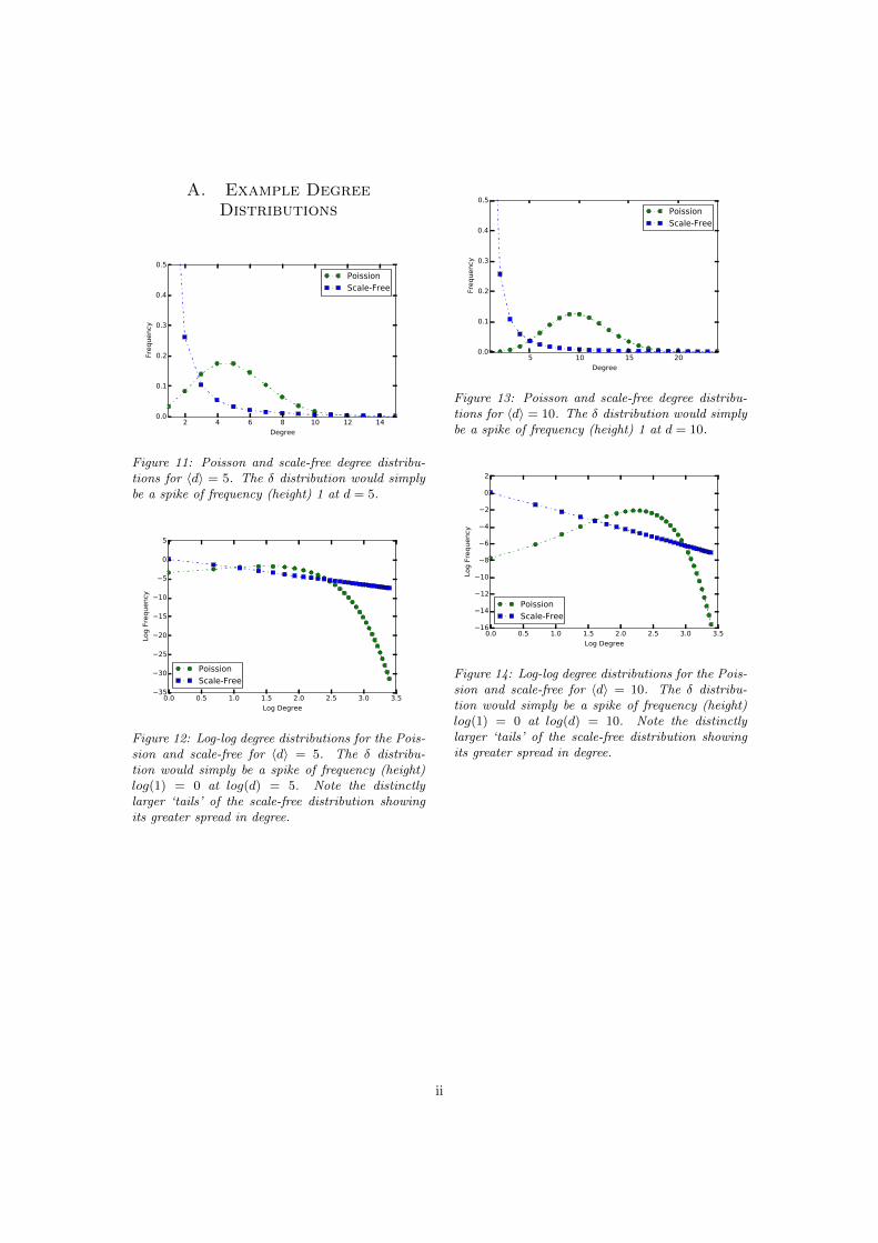
A. Example DegreeDistributions

Figure 11: Poisson and scale-free degree distribu-tions for hdi = 5. The � distribution would simplybe a spike of frequency (height) 1 at d = 5.

Figure 12: Log-log degree distributions for the Pois-sion and scale-free for hdi = 5. The � distribu-tion would simply be a spike of frequency (height)log(1) = 0 at log(d) = 5. Note the distinctlylarger ‘tails’ of the scale-free distribution showingits greater spread in degree.

Figure 13: Poisson and scale-free degree distribu-tions for hdi = 10. The � distribution would simplybe a spike of frequency (height) 1 at d = 10.

Figure 14: Log-log degree distributions for the Pois-sion and scale-free for hdi = 10. The � distribu-tion would simply be a spike of frequency (height)log(1) = 0 at log(d) = 10. Note the distinctlylarger ‘tails’ of the scale-free distribution showingits greater spread in degree.

ii

B. Stochastic Ordering

Stochastic Ordering is an attempt at orderingprobability distributions.14

First order stochastic dominance capturesthat one probability distribution is ”bigger” oris ”higher” than another; ‘rational agents’ bet-ting on outcomes betweens distibutions shouldalways choose the dominant distribution. Con-sider two probability distributions (discrete orcontinuous) P (d) and eP (d). P (d) first orderstochastically dominates eP (d) if

Xf(d)P (d) �

Xf(d) eP (d),

for all nondecreasing functions15 f .P (d) can be formed by shifting probability

mass/weight upwards/to-the-right on the eP (d)distribution.

Second order stochastic dominance capturesthat P (d) has at least a high mean as eP (d) butis more centralised on a single value and so morepredictable. P (d) second order stochasticallydominates eP (d) if

Xf(d)P (d) �

Xf(d) eP (d),

for all nondecreasing, concave functions16 f .First order stochastic dominance implies secondorder.

A mean-preserving spread is a special caseof a distribution eP (d) being second order domi-nated by P (d) in which they have equal means;

hdi = fhdi. It removes the first order ‘part’ (i.ejust simply higher gains) and accentuates thepredictability due to spread part. It implies

Xf(d)P (d) �

Xf(d) eP (d),

for all concave functions f , and similarlyX

f(d)P (d) X

f(d) eP (d),

for all convex functions f .These are stated without proof but with

self-persuasion of their validity. The secondmoment of the degree of the network hd2i =P

d

P (d)d2 is the weighted sum over the con-vex function f(d) = d2 and so hd2i increaseswith increasing spread of P (d) while holding itsmean constant.

14Only gives a partial ordering; for two distributions, neither may dominate the other.15Equivalent conditions:

•P

x

0 P (d) P

x

0eP (d) for all x,

•P1

x

P (d) �P1

x

eP (d) for all x.

16Equivalent conditions:

•P

f(d)P (d) P

f(d) eP (d) for all non-increasing, convex functions f ,

•P

x

z=0

Pz

d=0 P (d) P

x

z=0

Pz

d=0eP (d) for all x.

iii

C. Further SIS Results

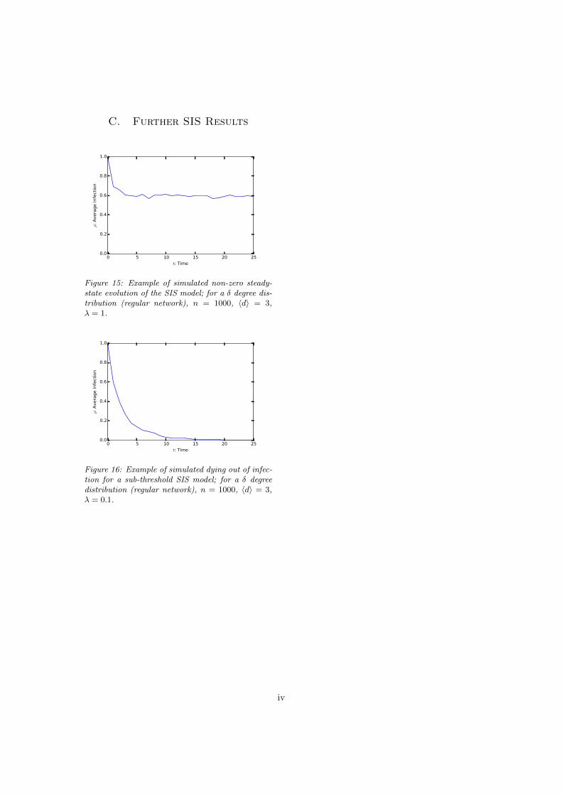
Figure 15: Example of simulated non-zero steady-state evolution of the SIS model; for a � degree dis-tribution (regular network), n = 1000, hdi = 3,� = 1.

Figure 16: Example of simulated dying out of infec-tion for a sub-threshold SIS model; for a � degreedistribution (regular network), n = 1000, hdi = 3,� = 0.1.

iv

D. Extended FinancialContagion Literature Review

1. Financial Contagion - Allen, Gale (2000)[20]. i) Research question: Can financial cri-sis be explain by contagion across a networkof banks. ii) General model : Static directed17

network of four banks. Links represent banklending. A pool of consumers that depositand withdraw funds in banks. System evolvesover a one-time series of events at t=0,1,2.Banks aim to maximise more profitable longerterm investment (from t=0 to t=2) of deposits,achieved through loaning along the designatedlinks. Loans are later liquidated in order toabsorb shorter term consumer withdrawals (att=1) as required. iii) Central quantities: Desig-nated network structure; completely connected,banks paired or a connected loop. Fractionof consumers making short term withdrawalsin each bank. iv) System shock : Single bankreceives an unexpectedly large withdrawal att=1 for which it currently does not have thefunds for, so goes insolvent and defaults on itsdebts. v) Contagion mechanism: Initial bankdefault transmits losses through the interbankloans (links) causing further possible insolven-cies. Call this mechanism counterparty loss.vi) Main results: It is possible to model fi-nancial collapse as contagion of bank defaulttransmitted through interbank loans. iv) Lim-itations: Model is overly specialised.

2. Network Models and Financial Stabil-ity - Nier et al. (2007) [21]. i) Researchquestion: How does the structure of financialnetworks a↵ect its susceptibility to systematicbreakdown. ii) General model : Static direc-tional and weighted18 ER network representingdirection and size of interbank loans betweenbanks. Banks hold a finite bu↵er against loss.iii) Central quantities: System size. Total eq-uity within system. Density of interbank loan-ing (link density). Average size of loans (aver-age link weight). Bank bu↵er size. iv) Systemshock : Set random bank as insolvent. v) Conta-gion mechanism: Counter party loss. Insolvent

banks default on all loans, transmitting lossesthrough interbank loans (links). Banks that re-ceive total losses greater than their bu↵er be-come insolvent. vi) Main results : Non-linearincrease in extent of contagion with decreas-ing bu↵er size. Non-monotonic change in ex-tent of contagion with increasing connectivity(link density). Extent of contagion normalisedby system size increases with decreasing systemsize. vii) Limitations : Shocks are both idiosyn-cratic and contained within a single bank, bothof which are not the case in practice. Only con-sidered di↵erent levels of connectivity within asingle network structure type.

3. Stability Analysis Of Financial Conta-gion due to Overlapping Portfolios - Caccioli etal. (2014) [23]. i) Research question: Given anetwork of leveraging19 banks with overlappingportfolios, how does the system’s stability toshocks change with varying system parameters.ii) General model : Non-directional weighted bi-partite20 random network. Links represent abank’s investment in an asset. Asset values de-preciate exponentially as banks liquidate them.Banks have a finite bu↵er against losses. Abank is solvent while its liabilities, proportionalto its leverage, is less than its total value of as-sets plus bu↵er. iii) Central quantities: Levelof leverage. Diversification; average number ofassets each bank invests in (average bank de-gree). Market crowding; ratio of number ofbanks to assets. iv) System shock : Set randombank as insolvent, or depreciate value of ran-dom asset. v) Contagion mechanism: Insolventbanks liquidate all their assets, thus drivingthose asset values down. This leads to furtherpossible insolvency of banks connected throughoverlapping assets (banks linked through a sin-gle asset). vi) Main results : It is possible tomodel financial collapse as contagion throughoverlapping portfolios. The contagion is self-reinforcing; if initial shock is not absorbed thenall banks in the connected network componentgo insolvent. Non-monotonic change in proba-bility of collapse with increasing diversification;lower and upper threshold on non-zero proba-

17Links are one way; it is no longer the case that g

ij

= g

ji

.18Links are associated with a weight; adjacency matrix g

ij

now contains a spectrum of values.19Using debt to finance assets. Banks with substantially higher debt than equity are considered to be highly

leveraged.20A bipartite network consists of two sets of nodes, and links are only formed between nodes in di↵ering sets.

v

bility (phase transitions). Decreasing marketcrowding generally lowers probability of col-lapse and changes positions of thresholds. Ex-tent of collapse and thresholds independent ofshock type. Their exists a threshold on lever-age for possibility of collapse. vii) Limitations :Passive portfolio management (static system).Doesn’t include the counter party loss channelof contagion.

vi

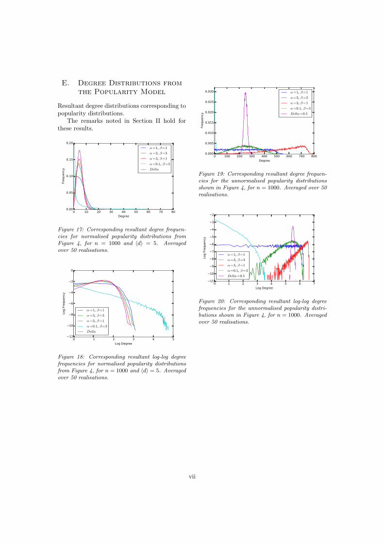
E. Degree Distributions fromthe Popularity Model

Resultant degree distributions corresponding topopularity distributions.

The remarks noted in Section II hold forthese results.

Figure 17: Corresponding resultant degree frequen-cies for normalised popularity distributions fromFigure 4, for n = 1000 and hdi = 5. Averagedover 50 realisations.

Figure 18: Corresponding resultant log-log degreefrequencies for normalised popularity distributionsfrom Figure 4, for n = 1000 and hdi = 5. Averagedover 50 realisations.

Figure 19: Corresponding resultant degree frequen-cies for the unnormalised popularity distributionsshown in Figure 4, for n = 1000. Averaged over 50realisations.

Figure 20: Corresponding resultant log-log degreefrequencies for the unnormalised popularity distri-butions shown in Figure 4, for n = 1000. Averagedover 50 realisations.

vii

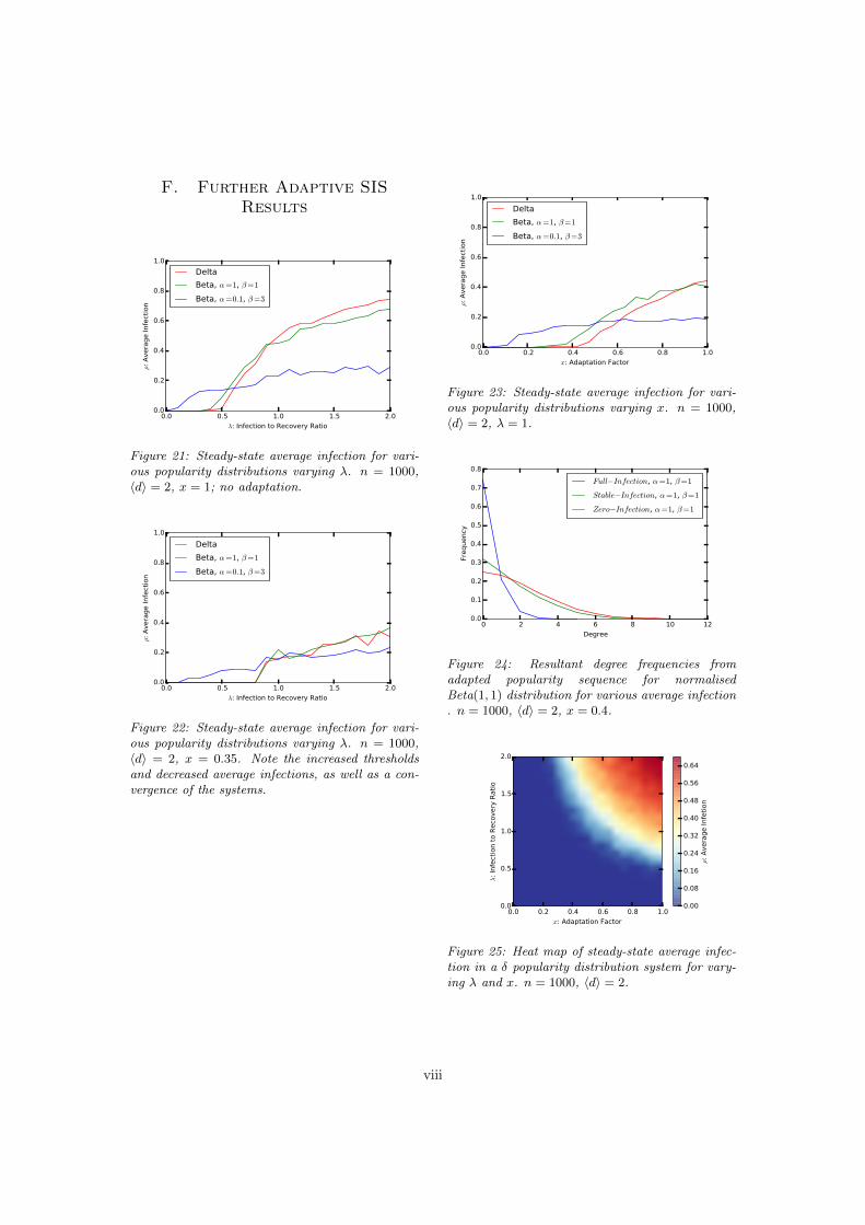
F. Further Adaptive SISResults

Figure 21: Steady-state average infection for vari-ous popularity distributions varying �. n = 1000,hdi = 2, x = 1; no adaptation.

Figure 22: Steady-state average infection for vari-ous popularity distributions varying �. n = 1000,hdi = 2, x = 0.35. Note the increased thresholdsand decreased average infections, as well as a con-vergence of the systems.

Figure 23: Steady-state average infection for vari-ous popularity distributions varying x. n = 1000,hdi = 2, � = 1.

Figure 24: Resultant degree frequencies fromadapted popularity sequence for normalisedBeta(1, 1) distribution for various average infection. n = 1000, hdi = 2, x = 0.4.

Figure 25: Heat map of steady-state average infec-tion in a � popularity distribution system for vary-ing � and x. n = 1000, hdi = 2.

viii

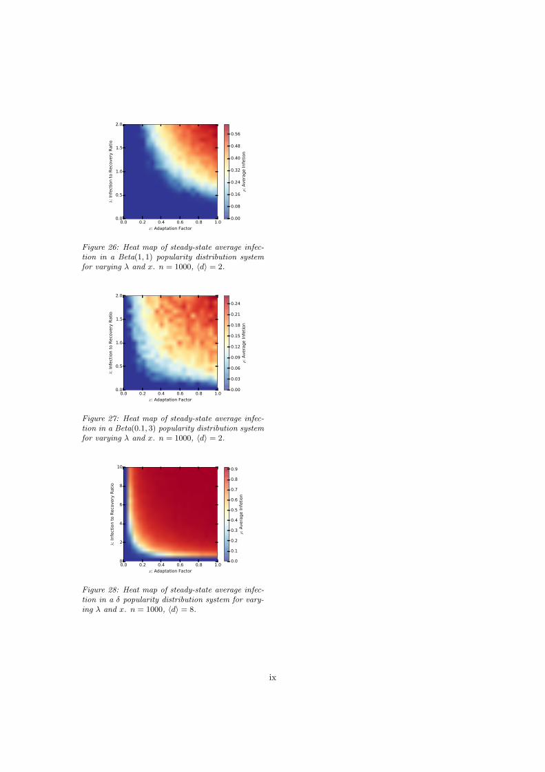
Figure 26: Heat map of steady-state average infec-tion in a Beta(1, 1) popularity distribution systemfor varying � and x. n = 1000, hdi = 2.

Figure 27: Heat map of steady-state average infec-tion in a Beta(0.1, 3) popularity distribution systemfor varying � and x. n = 1000, hdi = 2.

Figure 28: Heat map of steady-state average infec-tion in a � popularity distribution system for vary-ing � and x. n = 1000, hdi = 8.

ix

G. Simulations

All simulations and plots were written inPython. Below are links to iPython Notebookswhich contain complete code for each simula-tion, including explanatory comments.

• Degree Distribution Examples: resultsin Appendix A. https://gist.github.com/DBCerigo/30dea97eecc461300b08

• SIS Evolution: results in Appendix C.https://gist.github.com/DBCerigo/

0aeb443640ad86518d39

• SIS Thresholds: results in Figure 2.https://gist.github.com/DBCerigo/

c79b035be9a5cb428270

• SIS Steady-State Average In-fection: results in Figure 3.https://gist.github.com/DBCerigo/

8af94ff81f0132e03cef

• Popularity Model resultant Degree Dis-tribtuions: results in Figures 4, 5and 6, as well as results in Ap-pendix E. https://gist.github.com/

DBCerigo/461242a08f0d6c3bffc0

• Adaptive SIS Steady-State Average In-fections Varying Infection-Recovery Ra-tio �: results in Figures 7, 21, 22and 24. https://gist.github.com/

DBCerigo/ab04a3520960e699cfa4

• Adaptive SIS Steady-State Aver-age Infections Varying AdaptationFactor x: results in Figure 23.https://gist.github.com/DBCerigo/

8b3a220fa0262ba6ed89

• Adaptive SIS Heat Maps: results for allheat maps. https://gist.github.com/

DBCerigo/c6ad06a8d000b442af54

x